Embed Size (px)
Citation preview
AN ABSTRACT OF THE DISSERTATION OF
Yan Du for the degree of Doctor of Philosophy in Economics presented on August
1, 2008.
Title: Code-sharing in the U.S. Airline Industry
Abstract approved:
B. Starr McMullen
This dissertation consists of two essays that address code-sharing alliances
in the U.S. domestic airline industry.
The first essay examines the economic impact of code-sharing using data
from the complementary code-sharing agreement between Southwest and ATA
Airlines. This code-share agreement is found to decrease air fares and increase
passenger volumes for incumbent firms, while increasing both consumer and
producer surplus on code-shared routes to and from the Denver airport. In addition,
these markets are found to exhibit characteristics of Bertrand competition, as
opposed to previous findings of the less competitive Cournot result in international
markets and in other domestic U.S. markets.
The second essay employs three alternative econometric models
(Generalized Linear Mixed Models (GLIMM), Generalized Estimating Equations
(GEE) and Transition Models (TM)) analyze factors that determine whether
individual routes remain in or leave a code-share agreement. The code-share
alliance between Continental and America West Airlines is used as the case study
for this analysis. Empirical results show that routes with higher flight frequencies
and higher yields lead to a higher probability of remaining in the code-share
agreement. Alliance firms tend to code-share routes where the origin, connecting or
destination airport is one of their hub cities or the route is a vacation route. Airport
congestion and high route concentration are found to be important barriers that
limit use of code-sharing.
©Copyright by Yan Du
August 1, 2008
All Rights Reserved
Code-sharing in the U.S. Airline Industry
by Yan Du
A DISSERTATION
Submitted to
Oregon State University
in partial fulfillment of
the requirements for the
degree of
Doctor of Philosophy
Presented August 1, 2008
Commencement June 2009
Doctor of Philosophy dissertation of Yan Du presented on August 1, 2008.
APPROVED:
Major Professor, representing Economics
Director of the Economics Graduate Program
Dean of the Graduate School
I understand that my dissertation will become part of the permanent collection of
Oregon State University libraries. My signature below authorizes release of my
dissertation to any reader upon request.
Yan Du, Author
ACKNOWLEDGEMENTS
The author expresses sincere appreciation for the advising, support and
encouragement of Dr. B. Starr McMullen. Her patience and direction made the
completion of this dissertation possible.
I would like to thank Dr. Joe Kerkvliet, Dr. Andrew Stivers and Dr. Steve
Buccola for their valuable comments and suggestions in all aspects of this
dissertation.
I am also grateful for finance provided by William and Joyce Furman
Fellowships for research in Transportation Economics.
TABLE OF CONTENTS
Page
1. Introduction ………………………………………………………................. 1
2. Assessing the Economic Impact of Domestic Airline Code-sharing: A Case Study of the ATA and Southwest Airlines Agreement………………... 5 3. Determinants of Successful Code-sharing: A Case Study of Continental and America West Airlines…………………………………………………… 47 4. Conclusion……………………………………………………........................ 103
5. Bibliography ….……………………………………………………………... 106
7. Appendices………………………………………………………………….. 113
LIST OF FIGURES
Figure Page
2.1 Effects of Code Sharing on Incumbents’ P and Q ……………………….... 40
3.1 Firm 1’s Airline Hub-and-spoke System …………………………………... 57
3.2 Code-sharing Alliances under Airlines’ Hub-and-spoke Systems…............... 59
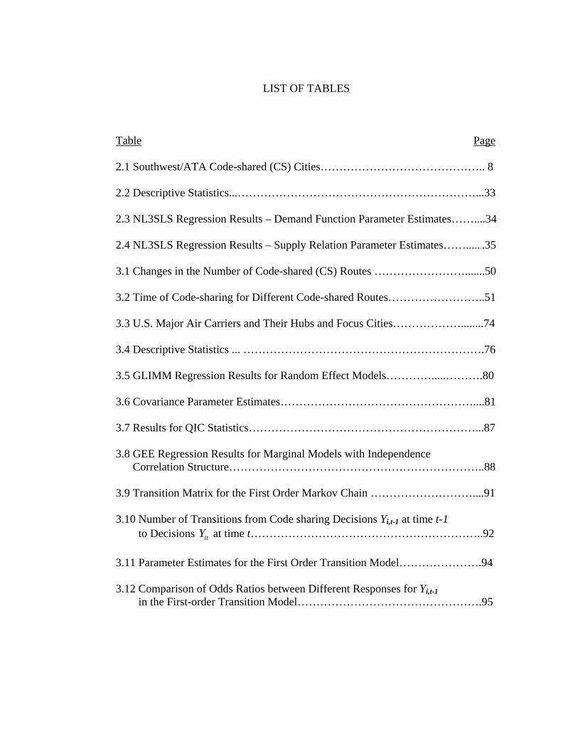
LIST OF TABLES
Table Page
2.1 Southwest/ATA Code-shared (CS) Cities…………………………………….. 8
2.2 Descriptive Statistics...………………………………………………………...33
2.3 NL3SLS Regression Results – Demand Function Parameter Estimates……....34 2.4 NL3SLS Regression Results – Supply Relation Parameter Estimates…….......35 3.1 Changes in the Number of Code-shared (CS) Routes …………………….......50
3.2 Time of Code-sharing for Different Code-shared Routes……………………..51
3.3 U.S. Major Air Carriers and Their Hubs and Focus Cities………………........74
3.4 Descriptive Statistics ... ……………………………………………………….76
3.5 GLIMM Regression Results for Random Effect Models………….....……….80
3.6 Covariance Parameter Estimates……………………………………………....81
3.7 Results for QIC Statistics……………………………………………………...87
3.8 GEE Regression Results for Marginal Models with Independence Correlation Structure…………………………………………………………..88 3.9 Transition Matrix for the First Order Markov Chain ………………………....91
3.10 Number of Transitions from Code sharing Decisions Yi,t-1 at time t-1 to Decisions at time t……………………………………………………..92 itY 3.11 Parameter Estimates for the First Order Transition Model………………….94
3.12 Comparison of Odds Ratios between Different Responses for Yi,t-1 in the First-order Transition Model………………………………………….95
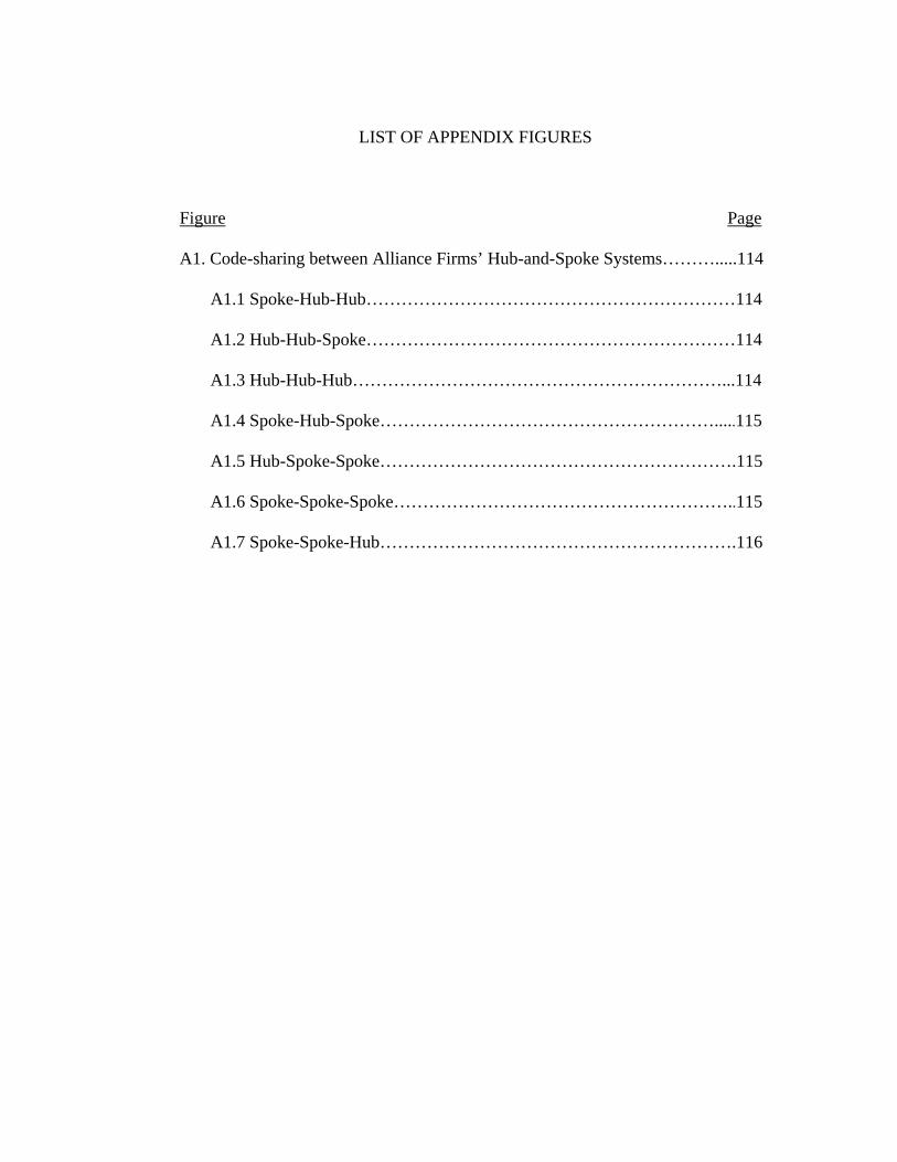
LIST OF APPENDIX FIGURES
Figure Page
A1. Code-sharing between Alliance Firms’ Hub-and-Spoke Systems……….....114
A1.1 Spoke-Hub-Hub………………………………………………………114
A1.2 Hub-Hub-Spoke………………………………………………………114
A1.3 Hub-Hub-Hub………………………………………………………...114
A1.4 Spoke-Hub-Spoke………………………………………………….....115
A1.5 Hub-Spoke-Spoke…………………………………………………….115
A1.6 Spoke-Spoke-Spoke…………………………………………………..115
A1.7 Spoke-Spoke-Hub…………………………………………………….116
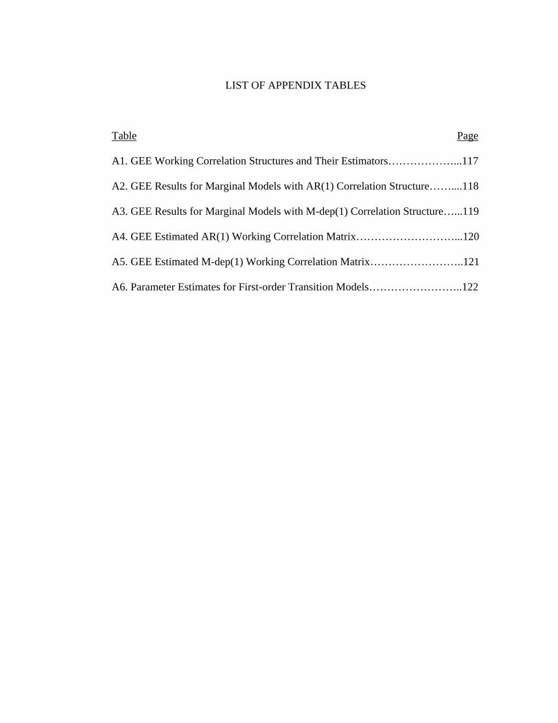
LIST OF APPENDIX TABLES
Table Page
A1. GEE Working Correlation Structures and Their Estimators………………...117
A2. GEE Results for Marginal Models with AR(1) Correlation Structure……....118 A3. GEE Results for Marginal Models with M-dep(1) Correlation Structure…...119 A4. GEE Estimated AR(1) Working Correlation Matrix………………………...120 A5. GEE Estimated M-dep(1) Working Correlation Matrix……………………..121 A6. Parameter Estimates for First-order Transition Models……………………..122
Code-sharing in the U.S. Airline Industry
Chapter 1
Introduction
2
This dissertation addresses issues of code-sharing alliances in the U.S.
airline industry. Under code-sharing, alliance firms merge their computer
reservation systems and each carrier can issue tickets on flights operated by other
contracting carriers by display of their own flight numbers. Since the first code-
sharing was implemented in the U.S. in the middle of the 1990’s, there has been a
heated discussion about the advantages and disadvantages of code-sharing alliances.
Alliance firms argue that code-sharing may bring benefits to customers because
code-sharing helps generate more flight options and connecting routes for
passengers. However, some airline researchers worry that code-sharing may
decrease competition between contracting carriers themselves and the competition
between code-shared firms and market incumbents.
In Chapter 2, we examine the economic impact of code-sharing on airfares,
passenger volumes and social welfare using data from the complementary code-
sharing agreement between Southwest and ATA Airlines. Previous studies
investigating the impact of code-sharing either on passenger volumes or air fares
have ignored the simultaneity between market demand and supply. Therefore,
results may not be consistent. Accordingly, we employ Bresnahan’s (1989)
conjectural variation (CV) approach to build a supply relation and demand function.
This approach allows us to test for market power in the market studied.
Empirical results from regressions using Nonlinear Three Stage Least
Squares (NL3SLS) show that the ATA/Southwest code-share agreement decreased
air fares and increased passenger volumes for incumbent firms. Further, both
3
consumer and producer surpluses increased on code-shared routes. Finally, these
markets were found to exhibit characteristics of Bertrand competition, as opposed
to previous findings of the less competitive Cournot result in international markets
and in other domestic U.S. markets. Our finding of Bertrand competition suggests
that previously expressed concerns regarding possible anti-competitive effects from
code-sharing are unwarranted in these markets.
In Chapter 3, we examine the determinants of successful code-sharing
alliances. Since the implementation of the first code-sharing agreement, code-
sharing has become increasingly popular in the U.S. airline industry. However,
alliance firms keep changing their code-shared route arrangements, adding new
routes and dropping the old ones. In Chapter 3 we present a theoretical model in
which two equilibrium conditions are derived: one showing when code-shared
firms will initially enter a code-share alliance and the other indicating conditions
when partner firms will choose to remain in or exit a particular code-shared route
after the initial entry. The empirical part of this paper uses discrete longitudinal
analysis to examine the code-sharing agreement between Continental and America
West. We employ three alternative econometric models (Generalized Linear Mixed
Models (GLIMM), Generalized Estimating Equations (GEE) and Transition
Models (TM)) for the analysis. Empirical results show that routes with higher flight
frequencies and higher yields lead to a higher probability of remaining in a code-
share agreement. Alliance firms tend to code-share routes where the origin,
connecting or destination airport is one of their hub cities or the route is a vacation
4
route. Airport congestion and high route concentration are found to be important
barriers that limit use of code-sharing. Population and income in the origin and
destination metropolitan statistical areas are also important factors affecting firms’
code-sharing decisions.
Chapter 4 summarizes the study conclusion and provides a discussion of
policy implications.
5
Chapter 2
The Economic Impact of the ATA/Southwest Airlines Code-share Alliance - a Case Study from Denver International Airport
6
I. Introduction
In October 2004, ATA Holdings and its subsidiaries filed for Chapter 11
bankruptcy protection. 1 Subsequently, Southwest Airlines injected capital into
ATA Airlines that resulted in Southwest having a 27.5% ownership stake in ATA
upon their exit from Chapter 11 bankruptcy proceedings. As part of the deal,
Southwest entered into a code-sharing arrangement with ATA. This was
Southwest’s first domestic code-sharing arrangement. ATA chose 11 cities that had
not been served by Southwest as the code-sharing cities with Chicago Midway
Airport as the connecting airport for both airlines. Southwest cities that were part of
the code- share agreement are listed in Table 2.1.
Southwest Airlines is based in Dallas, Texas. It is the third largest airline in
the world, measured in terms of the number of passengers carried, and the largest
with destinations exclusively in the United States. Despite the restrictions on its
home base, Dallas Love Field, since 1978, Southwest has built a successful
business by flying multiple short quick trips into the secondary airports of major
cities using primarily Boeing 737 aircraft.2 ATA Airlines is an American low cost
1 “Chapter 11 is a chapter of the United States Bankruptcy Code which governs the process of reorganization under the bankruptcy laws of the United States. The Bankruptcy Code itself is Title 11 of the United States Code; therefore reorganization under bankruptcy is covered by Chapter 11 of Title 11 of the United States Code. In contrast Chapter 7 governs the process of a liquidation bankruptcy.”
2 When airline deregulation came in 1978, Southwest began planning to offer interstate service from Dallas Love Field (DAL), but a number of interest groups affiliated with DAL Airport, including American Airlines and the city of Fort Worth, pushed the Wright Amendment through Congress to restrict such flights. Southwest was barred from operating, or even ticketing passengers on flights from
7
and charter airline based in Indianapolis, Indiana. ATA operates scheduled
passenger flights from a hub at Midway Airport in Chicago, Illinois, and charter
flights across the globe.
As a low-cost air carrier, Southwest is well known as a "discount airline"
compared to its domestic rivals and it is the only U.S. airline which has been
profitable every year since 1973. Past studies of Southwest deal with various
aspects of Southwest’s entry or potential entry on pre-existing market behavior
such as Bennet and Craun (1993), Morrison (2001), Boguslaski, Ito and Lee (2004)
and Fu, Dresner and Oum (2006). Most find that entry or potential entry by
Southwest into a market significantly lowers market fares, which is the well known
“Southwest Effect”.
The purpose of this paper is to examine the impact of the 2005 code-sharing
agreement between Southwest and ATA on air fares and passenger volumes in the
Denver markets. What is unique about this code share agreement is that it is the
first time that Southwest has entered a market in this way. While it is clearly a
complementary code-sharing agreement, there is the question of whether this
Love Field beyond the states immediately surrounding Texas. In 1997, the Shelby Amendment added the states of Alabama, Mississippi, and Kansas to the list of permissible destination states. Since late 2004, Southwest has been actively seeking the full repeal of the Wright Amendment restrictions. In late 2005, Missouri was added to the list of permissible destination states via a transportation appropriations bill. New service from Dallas Love Field to St. Louis and Kansas City quickly started in December of 2005. In 2006, Southwest and American Airlines both required approval from the Federal Aviation Administration to begin one-stop flights from Love Field to destinations outside the Wright limits. In October 2006, Southwest announced that it would begin one-stop or connecting service between Love Field and 25 destinations outside the Wright zone.
8
Table 2.1 Southwest/ATA Code-shared (CS) Cities
Southwest CS City ATA City Southwest Non-CS City Albuquerque Boston Albany Baltimore Washington Denver Amarillo Birmingham Ft Myers Naples Austin Cleveland Honolulu Boise Columbus Minneapolis St Paul Buffalo Detroit Metro Newark Burbank Ft Lauderdale Hollywood New York LaGuardia Corpus Hartford Springfield San Francisco Dallas Houston Sarasota Bradenton Dulles Indianapolis St Fetersburg El Paso Jackson Washington National DC Harlingen Jacksonville Lubbock Kansas City Midland/Odessa Las Vegas Norfolk Little Rock Orange County Long Island Macarthur Pittsburgh Los Angeles Reno Louisville Salt Lake City Manchester San Antonio Nashville San Jose New Orleans Spokane Oakland Oklahoma City Omaha Ontario Orlando Philadelphia Phoenix Providence Raleigh Durham Sacramento San Diego Seattle St Louis Tampa Bay Tucson Tulsa West Palm Beach
9
agreement will have the same impact on fares and competition that Southwest’s
direct entry has had in other markets. From a policymaker’s point of view, code-
sharing alliances should be implemented if they have a net positive impact on
social welfare. The purpose of this paper is to provide policymakers additional
information on which to assess the effects of this code share agreement.
The next section provides a review of the literature on code-share
agreements, followed by presentation of the theoretical model. Section III explains
the empirical model and Section IV details the data sources. The empirical results
are then presented and discussed, followed by future research plans.
II. Background on Code-sharing Alliances
Code-sharing alliances began on international airline routes in 1986 and by
the end of the 1990s had become one of the most popular alliance forms in the
airline industry. Generally speaking, code-sharing arrangements have two basic
forms: complementary and parallel alliances. Complementary alliances occur when
contracting air carriers link existing flight networks, resulting in a new
complementary network to provide services for connecting passengers (Park, 1997).
On the other hand, parallel (or overlapping) alliances refer to collaboration between
contracting air carriers competing on the same flight routes.
In the case of the ATA/Southwest code-share agreement, we are mostly
dealing with complementary alliances. In this case, there is no concern that the
agreement is eliminating an existing competitor as could be the situation with a
parallel agreement.
10
Code-shared flights have several advantages for both alliance firms and
passengers. First, the connecting flight is listed as a single-carrier flight under
either the ticketing or operating airline’s designation code and thus appears before
listings of interline connections on Computer Reservation System (CRS) screens.3
This listing priority can give alliance airlines an advantage over their competitors.
Second, code-shared flights can provide as much convenience as a single-carrier
flight. Customers only need to buy a single ticket for the entire route and their
baggage will be transferred at the connecting airport by airline employees. Third,
code-sharing combines alliance airlines’ current route networks and consequently
results in a substantial increase in the number of flight options that partner airlines
can offer without adding additional aircraft departures.
Thus, alliance firms can benefit by generating additional passengers who
might otherwise have chosen direct flights or flown through other hubs served by
competitors in the absence of code-sharing. These expanded service options may
attract new passengers and result in alliance firms coordinating and offering more
frequent flights, thus attracting even more passengers. In the presence of economies
of density, domestic traffic gains from code-sharing alliances may help lower the
3 Airline designation codes are two-letter codes assigned by the IATA
(International Air Transport Association), which form the first two letters of a flight code. They are listed for use in reservations, timetables, tickets, tariffs, air waybills and in airline interline telecommunications, as well as in the airline industry applications.
11
marginal operating cost of carrying an additional passenger.4 In addition, joint use
of airport facilities and development of new routes that may restructure the current
network may also reduce costs. Therefore, partner airlines may be able to lower air
fares to passengers as a result of the code sharing alliance.
However, it has also been argued that code-sharing may harm market
competition and decrease consumer welfare. According to the U.S. General
Accounting Office (1998), the listing priority given code-shared flights on the CRS
screen may decrease market competition with competitors operating on the same
routes. Second, although code-sharing is not regarded as a merger, it may reduce
the incentive for alliance partners to compete with each other on hundreds of
nonstop, one-stop or multiple-stop long-haul markets. Currently these routes are the
most competitive markets because they offer the greatest number of airlines from
which consumers can choose. If the alliance airlines successfully gain market share,
market incumbents could be driven out and entry could become more difficult.
Limited competition and increased market concentration on these routes could
result in an increased possibility of collusion, leading to airfare increases and
decreases in service quality. Thus, it is possible that code-sharing agreements could
have a negative impact on customers and incumbent carriers.
4 Economies of density mean that within a network of given size, increases in the size of aircraft will lead to a decrease in unit cost. Please see Caves, Christensen, Tretheway (1984) and Oum and Tretheway (1982) for details.
12
Most studies of code-sharing alliances have involved international code-
sharing practices. Oum, Park and Zhang (1996), Park (1997), Park and Zhang
(2000), Park, Zhang and Zhang (2001), Park, Park and Zhang (2003), Brueckner
and Whalen (2000), Shy (2001), Brueckner (2001, 2003), Hassin and Shy (2004)
examine the impact of international code-sharing alliances on firm output, air fares
and economic welfare, either empirically or theoretically. Almost all of these found
that complementary international code-sharing alliances are likely to increase
passenger volumes, decrease air fares and improve consumer welfare.
To date, studies of domestic code-sharing and its competitive effects
include Bamberger, Carlton and Neumann (2004), Armantier and Richard (2005a,
2005b), Chua, Kew and Yong (2005) and Gayle (2006). Bamberger, Carlton and
Neumann (2004) find that complementary code-sharing between Continental and
America West decreases average air fares and increases total traffic in a code-
shared market while Gayle (2006) predicted that alliance firms’ air fares would fall
after a parallel code-sharing agreement between Continental, Delta and Northwest
was proposed in 2002. Armantier and Richard (2005a) find that air fares increased
significantly in markets where partner firms (Continental (CO) and Northwest
Airlines (NW)) offered code-shared flights and had nonstop direct flights as well,
whereas air fares were lower in markets where firms code-shared flights but did not
operate any nonstop flight. Armantier and Richard (2005b) further find that
consumer surplus per passenger falls after code-sharing between CO and NW.
Chua, Kew and Yong (2005) use firm-specific panel data to assess the impact of
13
code-sharing on operating cost and find that large alliance partners have a negative
effect while small alliance partners have a positive effect on firm operating costs.
This paper will make several contributions to the existing literature: It is the
first to analyze U.S. complementary code-sharing by estimating both demand and
supply sides simultaneously. It is also the first to analyze the effect of code-sharing
between two U.S. low cost air carriers on the market incumbents. Previous
researchers have examined code sharing alliances between U.S. legacy air carriers.
But, low cost carriers are known to have different business model practices than
legacy carriers.5 The case studied here is unique in that this is Southwest’s code
sharing with ATA, the first domestic code sharing alliance that Southwest has
entered. Although many previous studies of market power in the airline industry
such as Brander and Zhang (1990, 1993), Oum, Zhang and Zhang (1993), Park and
Zhang (2000), Fischer and Kamerschen (2003) assume product homogeneity, this
is generally not the case in the airline industry. Important service quality
differences may take the forms of flight frequency, on-time performance such as
arrival and departure delay, air time, ground transportation availability, advertising,
departure schedule, day of the week and safety and accident reputation. Oum, Park
and Zhang (1996) and Borenstein and Netz (1999) find that either flight frequency
5 In contrast to legacy carriers who are usually engaged in complicated yield management, operating practices of low cost air carriers include: a) a single passenger class, b) a single type of air plane, reducing training, servicing and maintenance costs, c) a simple fare scheme, d) flying to cheaper, less congested secondary airports and flying early in the morning or late in the evening to avoid air traffic delays and take advantage of lower landing fees, e) short flights and fast turnaround times.
14
or departure time is significantly different across firms. Thus, we assume product
differentiation in this study of how individual incumbents responded to the
Southwest and ATA code-sharing strategy.
III. Theoretical Model
We follow previous researchers (Brander and Zhang (1990, 1993), Oum,
Park and Zhang (1996), Captain and Sickles (1997) and Fischer and Kamerschen
(2003)) and use a general conjectural variation reduced form approach. The basic
model was originally suggested by Iwata (1974) and later extended and generalized
by Bresnahan (1989). This methodology allows us to find the average degree of
market power and estimate the price-cost margin while imposing less demanding
data requirements than a structural conjectural variation model. Further, instead of
regarding the conjectural variation as a firm’s expectation, it can be interpreted as
“a market parameter to capture the whole range of market performance and
dynamic patterns can be approximated by repeated, one-shot static equilibrium
game” in the airline industry (Fischer and Kamerschen, 2003).
In this paper, we regard a city-pair flight route as a market and assume that
n incumbent airlines (firm i=1,…n) offer flight services. Further, we assume that
the passenger volume demanded from each incumbent air carrier is a function of its
own air fare, its competitors’ air fares and other exogenous variables that affect its
demand. Then incumbent firm 1’s inverse market demand function can be written
as:
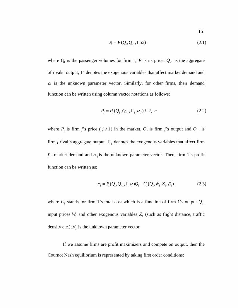
15
1 1 1 1( , , , )P P Q Q α−= Γ (2.1)
where is the passenger volumes for firm 1; 1Q 1P is its price; is the aggregate
of rivals’ output; denotes the exogenous variables that affect market demand and
1Q−
Γ
α is the unknown parameter vector. Similarly, for other firms, their demand
function can be written using column vector notations as follows:
( , , , )j j j j j jP P Q Q α−= Γ j=2,..n (2.2)
where jP is firm j’s price ( 1j ≠ ) in the market, jQ is firm j’s output and jQ− is
firm j rival’s aggregate output. jΓ denotes the exogenous variables that affect firm
j’s market demand and jα is the unknown parameter vector. Then, firm 1’s profit
function can be written as:
1 1 1 1 1 1 1 1 1 1( , , , ) ( , , , )P Q Q Q C Q W Zπ α β−= Γ − (2.3)
where stands for firm 1’s total cost which is a function of firm 1’s output ,
input prices and other exogenous variables
1C 1Q
1W 1Z (such as flight distance, traffic
density etc.); 1β is the unknown parameter vector.
If we assume firms are profit maximizers and compete on output, then the
Cournot Nash equilibrium is represented by taking first order conditions:
16
'11 1 1 1 1 1
1
1 11 1 1
1 1
1 11 1
21 1 1
11 1 1 1
1
( , , , )
=
=
= (1 )
=0
nj
j
P Q P Q Q cQ
P QP Q cQ Q
QP QP Q cQ Q Q
PP Q v cQ
π α−
−
=
∂= + Γ −
∂
⎛ ⎞∂ ∂+ + −⎜ ⎟∂ ∂⎝ ⎠
∂⎛ ⎞∂ ∂1+ +⎜∂ ∂ ∂⎝ ⎠
∂+ + −
∂
∑ −⎟ (2.4)
11
1
where QvQ−∂
=∂
and stands for the marginal cost of firm 1. 1c
So 11 1 1 1
1
(1 ) 0 PP Q v cQ∂
+ + −∂
= (2.5)
In the symmetric oligopoly model, equals 0 for Cournot competition; equals
-1 for Bertrand competition and equals 1 for the cartel solution. Because we do
not know whether the firms are competing on output or price, or whether they are
colluding, we have to adopt more general supply relations to describe the quantity
or price setting conduct and other oligopoly behaviors generalized by Bresnahan
(1989) as follows:
1v 1v
1v
11 1 1
1
PP c QQ 1λ∂
= −∂
(2.6)
where 1 11 vλ = + ( 1 0λ ≥ ) is defined as the market power parameter. As 1λ moves
17
farther from 0, the conduct of firm 1 moves farther from perfect competition.
Accordingly, firm j’s supply relation can be written as:
jj j j
j
PP c Q
Q jλ∂
= −∂
(2.7)
One way to measure the effect of code-sharing on the market incumbents’ prices
and passenger volumes is to estimate the n structural demand equations (2.1)-(2.2)
and supply relations (2.6)-(2.7) simultaneously as a system of equations, with code-
sharing as an explanatory variable.
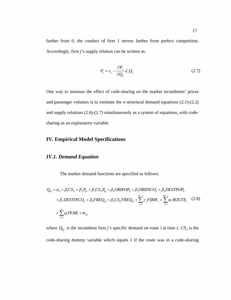
IV. Empirical Model Specifications
IV.1. Demand Equation
The market demand functions are specified as follows:
0 1 2 3 4 5 6
1 1
7 8 91 1
2
1
ijt it ijt it ijt it it it
N M
it ijt it ijt j j i ij i
t t ijtt
Q CS P CS P ORIPOP ORIINCO DESTPOP
DESTINCO FREQ CS FREQ FIRM ROUTE
YEAR
α β β β β β β
β β β γ ψ
ϕ ϖ
− −
= =
=
= + + + + + +
+ + + + +
+ +
∑ ∑
∑
(2.8)
where is the incumbent firm j’s specific demand on route i at time t; is the
code-sharing dummy variable which equals 1 if the route was in a code-sharing
ijtQ itCS
18
arrangement in 2005, and equals 0 if not.6 We expect the coefficient of to be
negative because code sharing offers passengers more flight options and thus may
decrease market demand for incumbent airlines’ services. However, incumbents
may also make full use of their frequent flyer program or increase their departure
frequency to attract more passengers and thus possibly increases their demand.
Compared with code-sharing services, incumbents’ nonstop flights are of higher
service quality. In this case, code sharing may indirectly increase incumbents’
demand so the coefficient sign may also be positive. is firm j’s air fare on route
i at time t and we expect this coefficient to be negative. captures the
interaction between code-sharing and firm j’s air fare. We expect this coefficient
sign to be negative because code sharing service can work as a substitute, thus
making incumbent firm j’s passengers more responsive to firm j’s price
changes. ,
itCS
ijtP
it ijtCS P
itORIPOP itDESTPOP are exogenous variables defined as the population
of the origin and destination metropolitan statistical areas and their coefficients are
expected to be positively related to the market demand.
Similarly, ,itORIINCO itDESTINCO are defined as the per capital incomes of the
6 There are some concerns that alliance firms may choose to code share in thick markets, which brings about the endogeneity issue of code sharing in the demand equation. However, in the case of code-sharing between ATA and Southwest, the code sharing route arrangement was made and implemented at the beginning of 2005, so the passenger volumes and air fares from 2005 should not be considered as factors that affect alliance firms’ decisions. Correlation test shows that there is no significant linear correlation between code sharing decisions and passenger volumes in 2003, 2004 and 2005 respectively. The descriptive statistics shows that both in 2003 and 2004, incumbents’ passenger volumes on the routes that were chosen for code-sharing in 2005 were fewer than those on the routes that were not.
19
origin and destination cities, respectively with coefficients expected to be positive
for normal goods and negative for interior goods.
Flight frequency is one of the most important elements that affect airline
demand and service quality.7 Passengers usually prefer airlines that offer more
frequent flights and thus reduce schedule delay time. So we include (the
number of firm j’s performed departures on route i at time t) and expect its
coefficient to be positively related to the demand. captures the
interaction between code-sharing and firm j’s departure frequency on route i at time
t and we expect the coefficient sign to be positive if code-sharing between code
sharing helps increase incumbent firm j’s departure frequency and negative if
decrease incumbent’ firm j’s departure frequency.
ijtFREQ
it ijtCS FREQ
jFIRM , and
are dummy variables that account for unobserved firm, route and time specific
fixed effects, respectively.
iROUTE tYEAR
ijtϖ is the normally distributed error term that might be
contemporaneously correlated across equations.
IV.2. Supply Relation 7 There is a possibility that flight frequency is endogenous because as the air travel demand increases, airlines may offer more frequent flight departures. However, Wald test (Green, 2003) shows the null hypothesis that flight frequency is exogenous can not be rejected: Wald statistics=1.3859945, which is less than 5.02 critical value at 5% confidence interval. We use the predicted value of flight frequency as the instrument in the test and least square estimates for the predicted value are good with high adjusted R square =99.96%. Possible reasons for the exogeneity of flight frequency can be that as the air travel demand increases, airlines tend to adopt larger aircrafts with more seats to avoid more landing and take-off fees associated with the increasing number of departures given that the airport capacity is limited as well.
20
To estimate the supply relation equation (2.4), we need to consider the
marginal cost function. However, precise definition and estimation of marginal cost
ses of this study, we need to specify marginal costs at the route
level. It is generally accepted that the airline industry is characterized by constant
on for an individual firm j on a
specific route i at time t as:
is problematic for the airline industry. Researchers have addressed airline costs in a
variety of ways. Brander and Zhang (1990, 1993), use average cost as a proxy for
marginal costs, a method later adopted by Oum, Zhang and Zhang (1993) and
Morrison and Winston (1995). However, most of these papers estimate the firm-
specific total and marginal cost on a domestic system-wide level rather than on the
specific route level.
For the purpo
returns to scale technology (CRS). This conclusion is supported by previous
researchers (Caves (1962), Eads, Nerlove and Raduchel (1969), Douglas and Miller
(1974), Keeler (1978), Caves, Christensen and Tretheway (CCT, 1984), Gillen,
Oum and Tretheway (1990), Oum and Zhang (1991), Brueckner and Spiller (1994)
and Creel and Farell (2001)). However, CRS assumption is not appropriate on the
route level. On a specific route, the more passengers an airline’s aircraft carries, the
lower the marginal cost given that the number of flight departure does not change.
We refer this as the economies of aircraft size, which is the reason for the existence
of economies of traffic density (Morrison, 2006).
Thus, we specify the marginal cost functi
21
2 3 4 5 6 7 8
1'
F L K Mijt ijt ijt jt jt ijt i ijt
N M
j j
1 2' '
1 1 1i i t t
j i t
MC W W W W CRAFTSIZE DIST Q
FIRM
χ χ χ χ χ χ χ
γ− −
= + + + + + +
+ +∑ ∑ ROUTE YEARψ ϕ= = =
+∑ (2.9)
here is the average fuel price measured as dollars per gallon for firm
route i at time t;8 is the average labor price measured by employees’ average
w j on FijtW
LijtW
hourly wage rate---dollars per worker for firm j on route i at time t;9 KjtW is the
capital input price defined as firm specific capital cost per unit of airline capacity
(available seat miles) at time t; 10 MjtW is the material input price measured by firm
specific material cost per available seat mile which, except fuel, labor and capital
8 Since some air carriers, especially large air carriers use contfuels to decrease their fuel cost, average fuel prices are actually different across airlines especially between large airlines and small ones. Moreover, according to
cial report shows that labor cost is different cross airlines as well. Following the same logic, we make some regional
a
ractual or storage
Petroleum Marketing Annual published by Energy Information Administration, Office of Oil and Gas, US Department of Energy, fuel prices are also different across regions and states. Thus, after regional and firm adjustments, average fuel prices change with routes, firms and time. Please refer to Section V for detailed descriptions of adjustment calculation.
9 According to Bureau of Transportation Statistics, US Department of Transportation, individual firm’s finanadjustment of firm level labor cost based on the Occupational Employment
Statistics (OES) Annual Survey provided by Bureau of Labor Statistics, US Department of Labor at the website http:/stat.bls.gov/oes/home.htm. Please see Section V for details. 10Capital cost are the total cost of operating property and equipments which include flight equipment, ground property and equipment, and leased property under capital
ases. We assume capital input prices do not change with flight routes. There is an lealternative way to measure the capital input prices and will be adopted when the data are available in the future research. Please see Section V for details.
22
costs, includes all the other expenditures such as maintenance, passenger food,
advertising, insurance, communication, traffic commissions and etc;11 We expect
the coefficient signs of these four input prices to be positively related to the
marginal cost. ijtCRAFTSIZE is the average number of available seats per aircraft
operated by firm at time t and we expect the sign of its coefficient to be
negative because the larger the number of seats, the larger the aircraft body size, the
lower the cost per passenger due to the economies of traffic density in the airline
industry and the lower the air fare is.
j on route i
12 iDIST is the distance of route i and we
expect its coefficient sign is positive because air fares are usually higher for longer
haul markets. ijtQ is the number of passengers carried by incumbent firm j on route
i at time t. W expect the coefficient on ijtQ to be negative because of the
economies of aircraft size (or economies of traffic density); however, if one more
additional passenger leads to crossing flights, then the marginal cost could increase
dramatically. Therefore, the overall effect is uncertain.
e
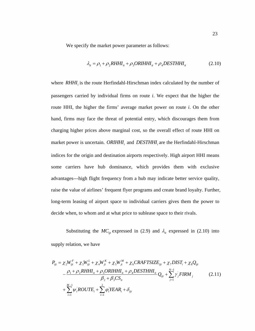
IV.3. Market Power Parameter Specification
11 We assume as well that airline firms buy those materials based on their whole system operation. Therefore, material input prices only change with firms and time but not with routes. Please see Section V for details. 12 Because firms operate different types of aircrafts on different routes at different time, and different types of aircrafts have a different number of available seats,
may also change with route, firm and time. Please see Section V for details.
ijtCRAFTSIZE
23
We specify the market power parameter as follows
S HHI
:
1 2 3 4it it itRHHI ORIHHI DE Tλ ρ ρ ρ ρ= + + + it (2.10)
e route Herfindahl-Hirschman index calculated b
ndividual firms on route i. We expect that the higher the
route HHI, the higher the firms’ average market power on route i. On the other
where iRHHI is th y the number of
passengers carried by i
hand, firms may face the threat of potential entry, which discourages them from
charging higher prices above marginal cost, so the overall effect of route HHI on
market power is uncertain. and iORIHHI iDESTHHI are the Herfindahl-Hirschman
advantages---high flight frequency from a hub may indicate better service quality,
raise the value of airlines’ frequent flyer programs and create brand loyalty. Further,
long-term leasing of airport space to individual carriers gives them the power to
decide when, to whom and at what price to sublease space to their rivals.
Substituting the ijt
indices for the origin and destination airports respectively. High airport HHI means
some carriers have hub dominance, which provides them with exclusive
MC expressed in (2.9) and itλ expressed in (2.10) into
supply relation, we have
2 3 4F L
ijt ijt ijtP W W Wχ χ χ= + + 5 6 7 8
1'1 2 3 4
12 3
1 2' '
1 1
K Mjt jt ijt i ijt
Nit it it
ijt j jjit
M
i i t t ijti t
W CRAFTSIZE DIST Q
RHHI ORIHHI DESTHHI Q FIRMCS
ROUTE YEAR
χ χ χ χ
ρ ρ ρ ρ γβ β
ψ ϕ δ
−
=
−
= =
+ + + +
+ + +− +
+
+ + +
∑
∑ ∑
(2.11)
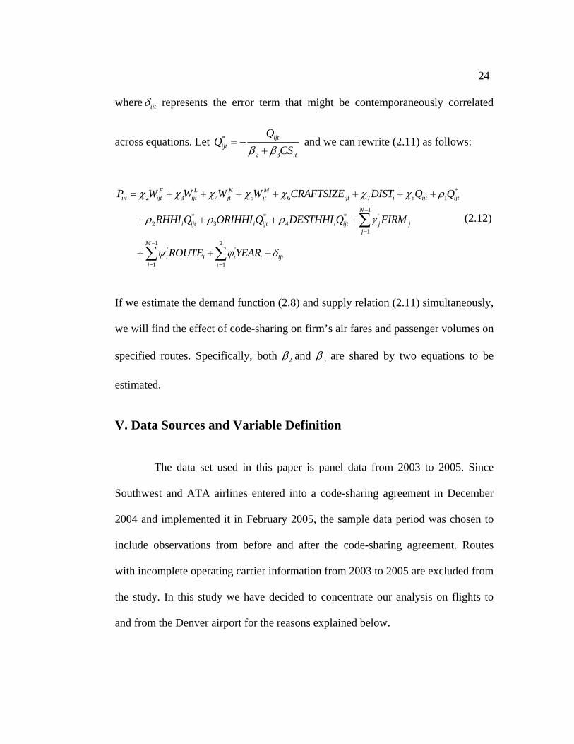
24
ijtδwhere represents the error term that might be contemporaneously correlated
across equations. Let *
2 3
ijtijt
it
CSβ β= −
+ and we can rewrite (2.11) as follows:
2 31
1 2'
1 1
F L K Mijt ijt ijt jt jt ijt i ijt ijt
j
M
t t ijti t
P W W W W CRAFTSIZE DIST Q Q
R
YEAR
χ χ χ χ χ χ χ ρ
ρ
ϕ δ
=
−
= =
= + + + + + + +
+∑
If we estimate the demand function (2.8) and supply relation (2.11) simultaneously,
we will find the effect of code-sharing on firm’s air fares and passenger volu
specified routes. Specifically, both
*2 3 4 5 6 7 8 1
1* * * '
4
'
N
i ijt i ijt i ijt j j
i i
HHI Q ORIHHI Q DESTHHI Q FIRM
ROUTE
ρ ρ γ
ψ
−
+ + + +
+ +
∑
∑
(2.12)
mes on
2β and 3β are shared by two equations to be
estimated.
V. Data Sources and Variable Definition
and ATA airlines entered into a code-sharing agreement in December
2004 and implemented it in February 2005, the sample data period was chosen to
ode-sharing agreement. Routes
with incom
The data set used in this paper is panel data from 2003 to 2005. Since
Southwest
include observations from before and after the c
plete operating carrier information from 2003 to 2005 are excluded from
the study. In this study we have decided to concentrate our analysis on flights to
and from the Denver airport for the reasons explained below.
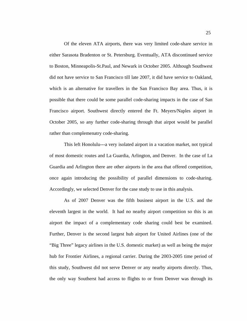
25
Of the eleven ATA airports, there was very limited code-share service in
either Sarasota Bradenton or St. Petersburg. Eventually, ATA discontinued service
to Boston, Minneapolis-St.Paul, and Newark in October 2005. Although Southwest
rts in the area that offered competition,
once a
amined.
did not have service to San Francisco till late 2007, it did have service to Oakland,
which is an alternative for travellers in the San Francisco Bay area. Thus, it is
possible that there could be some parallel code-sharing impacts in the case of San
Francisco airport. Southwest directly entered the Ft. Meyers/Naples airport in
October 2005, so any further code-sharing through that airpot would be parallel
rather than complemenatry code-sharing.
This left Honolulu---a very isolated airport in a vacation market, not typical
of most domestic routes and La Guardia, Arlington, and Denver. In the case of La
Guardia and Arlington there are other airpo
gain introducing the possibility of parallel dimensions to code-sharing.
Accordingly, we selected Denver for the case study to use in this analysis.
As of 2007 Denver was the fifth businest airport in the U.S. and the
eleventh largest in the world. It had no nearby airport competition so this is an
airport the impact of a complementary code sharing could best be ex
Further, Denver is the second largest hub airport for United Airlines (one of the
“Big Three” legacy airlines in the U.S. domestic market) as well as being the major
hub for Frontier Airlines, a regional carrier. During the 2003-2005 time period of
this study, Southwest did not serve Denver or any nearby airports directly. Thus,
the only way Southerst had access to flights to or from Denver was through its
26
code-share arrangement with ATA. Interestingly, Southwest later directly entered
Denver in January 2006, leading to speculation that the code-share arrangement
may have been a way to “test the waters” without incurring the costs of directly
entering the market at the outset.
Given data limitations on multiple stop flight services, we focus on the
routes where passenger volumes from direct flights account for more than 90% of
the total passenger volume.13 Therefore, our data sample includes 486 observations
V.1. Demand Function Variables
nd passenger volumes, are from
) US Department of Transportation (DOT)
Origin and Destination Survey DB1B Market, a 10% ticket random sample data.
ime
weighted average air fares of incumbent firm j on its non-stop market of route i at
across 68 routes to or from Denver International Airport, in which 19 routes were
code-shared by ATA and Southwest in 2005.
Firm specific average air fares, P aijt ijtQ
Bureau of Transportation Statistics (BTS
The number of passenger volumes used in the regression is ten t s that of
passenger volumes in the DB1B Market data. ijtQ is the number of passengers firm
j carries on its non-stop market of route i at time t while P is the passenger-
time t. Given the limit of data information, we cannot distinguish business-class or
ijt
13 We also examined the economic impact of code sharing between ATA and Southwest on the incumbent firms on those more comparable one-stop markets for the same route data sample, but most of the coefficient estimates are not statistically significant.
27
unrestricted coach class tickets from other tickets. Besides, we also include zero-
fare itineraries in the data sample. Code sharing routes ( itCS ) are identified from
Southwest Airlines News Releases “Southwest Airlines Announces Cities for Code-
share Flights with ATA Airlines” at http://www.southwest.com. ijtFREQ is defined
as the total number of departures performed by firm j on route i at time t and the
data are from BTS DOT Air Carrier Traffic Statistics T-100 Domestic Segment. To
make the characteristics of non code- shared routes comparable e of code
shared routes, we identify non code-shared routes as those with one end from
Denver, the city chosen by ATA for code sharing, and the other end is from
Southwest’s destination cities that were not included in the code share agreement.
The data for the population of origin and destination cities are from Population
Division US Census Bureau Annual Population Estimates of the Metropolitan
Statistical Areas. The data for the per capita personal income (in dollars) of origin
and destination cities are based on Metropolitan Statistical Areas level (MSA)
provided by Bureau of Economic Analysis, US Department of Commerce.
V.2. Supply Relation Variables
to thos
14
14The reason that we prefer to use population estimate by Metropolitan Statistical Areas (MSA) where either origin or destination city is located instead of population estimate by either origin or destination city only is due to the fact that the number of passengers may not be limited to the number of population in the departure city itself. Take Portland, Oregon for example: Besides the population of the Portland city itself, people around Portland such as those living in Beaverton Oregon may also choose Portland International Airport as the departure airport.
28
Fuel price, FijtW is regionally adjusted based on the average fuel price of
firm j at time t, ca ed by dividing the total domestic fuel cost of firm j by total
domestic gallons used by firm j in year t. Data for total domestic fuel cost and
obtained as
lculat
gallons are from BTS DOT Form 41 Air Carrier Financial Statistics Schedule P-
12A. Since some air carriers (especially large air carriers), may have contractual
and storage fuel advantages over small ones, firm level average fuel prices are not
completely the same as the concurrent market fuel prices and differences in average
fuel prices may exist between large and small air carriers. To control for regional
(state level) differences in average fuel prices, we normalize regional average fuel
prices to provide route and firm specific average fuel price. To illustrate how we do
this, suppose American Airlines’ (AA) average fuel price in all domestic operations
was $1.67 per gallon in 2005 and the average fuel price at the national level in 2005
was $1.74 per gallon. We take the national average fuel price as our base value and
calculate the regional average fuel price on the flight route, for example, from
Boston, MA (BOS) to Los Angles, CA (LAX) by taking the arithmetic means of
fuel prices from both the state of the origin city---MA and that of the destination
city---CA.15 Suppose the regional average fuel prices on the route BOSLAX we
get here is $1.70. Then, AA’s final average fuel price on the route BOSLAX is
1.701.67 1.6321.74
× = dollars per gallon in 2005. In this way, differences
in average fuel prices at route level are captured in addition to differences across 15 One assumption we make here is that air carriers add fuel at both origin and destination cities.
29
firms. Data f at both national and regional level (based on states)
by Energy Information Administration, Office of Oil and Gas, US Department of
We derive route level labor input prices LijtW for firm j on route i at time t
using a s
or the fuel prices
are available in the Petroleum Marketing Annual (2003, 2004 and 2005) published
Energy.
imilar normalization technique. We calculate firm level hourly average
wage per worker by dividing firm j’s total expenditure on salaries and related fringe
benefits by the product of total employees and working hours per year.16 The data
Schedule P-10 respectively. In order to take into consideration the regional
wage per worker, we choose the hourly average wage per worker in transportation
occupations at the national level as our base value and take the arithmetic means of
hourly average wage per worker. Then following the same logic as the calculation
hourly average wage per worker for a specific year. The data for the hourly average
wages at the national and MSA level are available in the Occupational Employment
are from BTS DOT Form 41 Air Carrier Financial Statistics Schedule P-6 and
(Metropolitan Statistics Area level---MSA level) differences in the hourly average
hourly average wages from the origin and destination MSA cities to obtain regional
of route level and firm specific average fuel price, we will have route and firm level
Statistics (OES) Survey (Nov 2003, Nov 2004 and May 2005 Estimates)
16 We assume 2,080 working hours for a full-time worker per year.
30
Transportation and Material Moving Occupation reported by Bureau of Labor
Statistics US Department of Labor.
Airline capital assets mainly include flight equipment, ground property and
quipm
Alternatively, we follow Chua, Kew and Yong (2005) and use total cost of
operati
Material input prices
e ent (GPE) such as maintenance and engineering equipment, ramp
equipment and other miscellaneous ground equipment, land, construction work in
progress, leased property under capital leases such as aircraft leases and etc.
Compared to aircraft expenditures, GPE costs are relatively small. Although we
would prefer to follow Oum and Yu (1998) and use aircraft lease rates as a proxy
for capital cost, this information was not available to us.
ng property and equipment per unit of airline capacity (measured by
available seat miles) that includes all the mentioned expenses above (GPE, land,
construction work and leased property under capital leases) less allowance for
depreciation as our firm level capital input prices. The data for the firm specific
capital cost and total number of available seat miles are available in BTS DOT
Form 41 Air Carriers Financial Statistics Schedule B-1 and BTS DOT Air Carrier
Traffic Statistics T-100 Air Carrier Summary T-2.
MjtW are calculated as a firm level materials and
t mservices cost per available sea ile. Materials and services cost includes all the
expenditures except fuel, labor and aircraft leasing cost, such as maintenance
materials, passenger food, advertising and promotions, communication and
31
insurance and etc. The data for the firm level total materials and services cost are
available in BTS DOT Form 41 Air Carrier Financial Statistics Schedule P-6. We
assume that airlines buy these materials and services based on their entire system
operations so the material input prices do not change with flight routes but only
change across airlines and time.
is measured as the average number of available seats per ijtCRAFTSIZE
aircraft operated by firm j on route i at time t. The larger the aircraft body size is,
the more available seats in the fleet. We use firm and route specific total number of
available seats divided by the total number of departures performed to get the
average number of available seats per aircraft. iDIST is the market distance
between the origin and destination cities and data ll of these variables are
available from the BTS DOT Air Carrier Traffic Statistics T-100 Domestic
Segment. itRHHI is the route Herfindahl-Hirschman index on route i. It is
calculated sum of the squares of the individual firms’ market share where
market share is calculated as the number of individual firm’s passengers divided by
the total number of passengers carried by all firms on route i. itORIHHI and
it
for a
by the
DESTHHI are the origin and destination airport Herfindahl-Hirsch
Following the same logic, they are calculated using the market share
of passengers originating (or arriving) at an airport for each carrier serving the
airport. All the data for the number of passengers carried by individual airlines are
man index
respectively.
32
available from Bureau of Transportation Statistics (BTS) US Department of
Transportation (DOT) Origin and Destination Survey DB1B Market.
All dollar values in the demand equation are deflated by the Consumer
Price Index (All Urban Consumers, All items, 1982-84=100) and those in the
supply equation are deflated by the Producer Price Index (All commodities, 1982-
84=100), obtained from the Bureau of Labor Statistics US Department of Labor.
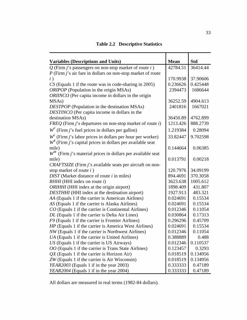
Descriptive statistics for all variables are listed in Table 2.2.
VI. Empirical Results
Empirical results are presented in Table 2.3 and Table 2.4 for both code-
shared and non code-shared routes to or from Denver airport. We estimate both
demand and supply functions simultaneously using Nonlinear Three State Least
Squares (NL3SLS). Instrument variables are all the remaining exogenous variables
in the equations.
VI.1. Demand Function
First, the estimate of air fares is negative as expected and statistically
significant at p=0.01 level. Second, compared to non code-shared routes, code-
sharing between Southwest and ATA significantly increases incumbents’ demand
by 162809 passengers per year. Thus, code-sharing between entrants does not
decrease passenger demand for incumbents’ flight services, a result consistent with
33
Table 2.2 Descriptive Statistics
Variables (Descriptions and Units) Mean Std
Q (Firm j’s passengers on non-stop market of route i ) 42784.51 36414.44P (Firm j’s air fare in dollars on non-stop market of route i ) 170.9938 37.90606CS (Equals 1 if the route was in code-sharing in 2005) 0.236626 0.425448ORIPOP (Population in the origin MSAs) 2394473 1686644ORIINCO (Per capita income in dollars in the origin MSAs) 36252.59 4904.613DESTPOP (Population in the destination MSAs) 2401816 1667021DESTINCO (Per capita income in dollars in the destination MSAs) 36450.89 4762.899FREQ (Firm j’s departures on non-stop market of route i) 1213.426 888.2739WF (Firm j’s fuel prices in dollars per gallon) 1.219384 0.28094WL (Firm j’s labor prices in dollars per hour per worker) 33.82447 9.702598WK (Firm j’s capital prices in dollars per available seat mile) 0.144664 0.06385WM (Firm j’s material prices in dollars per available seat mile) 0.013791 0.00218CRAFTSIZE (Firm j’s available seats per aircraft on non-stop market of route i ) 120.7976 34.09199DIST (Market distance of route i in miles) 894.4691 370.3058RHHI (HHI index on route i) 3623.638 1005.612ORIHHI (HHI index at the origin airport) 1898.409 431.807DESTHHI (HHI index at the destination airport) 1927.913 483.321AA (Equals 1 if the carrier is American Airlines) 0.024691 0.15534AS (Equals 1 if the carrier is Alaska Airlines) 0.024691 0.15534CO (Equals 1 if the carrier is Continental Airlines) 0.012346 0.11054DL (Equals 1 if the carrier is Delta Air Lines) 0.030864 0.17313F9 (Equals 1 if the carrier is Frontier Airlines) 0.296296 0.45709HP (Equals 1 if the carrier is America West Airlines) 0.024691 0.15534NW (Equals 1 if the carrier is Northwest Airlines) 0.012346 0.11054UA (Equals 1 if the carrier is United Airlines) 0.388889 0.488US (Equals 1 if the carrier is US Airways) 0.012346 0.110537OO (Equals 1 if the carrier is Trans State Airlines) 0.123457 0.3293QX (Equals 1 if the carrier is Horizon Air) 0.018519 0.134956ZW (Equals 1 if the carrier is Air Wisconsin) 0.018519 0.134956YEAR2003 (Equals 1 if in the year 2003) 0.333333 0.47189YEAR2004 (Equals 1 if in the year 2004) 0.333333 0.47189
All dollars are measured in real terms (1982-84 dollars).
34
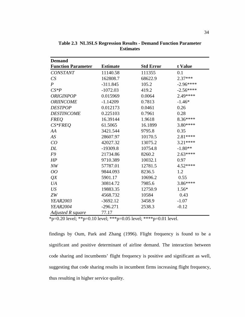
Table 2.3 NL3SLS Regression Results - Demand Function Parameter Estimates
Demand Function Parameter Estimate Std Error t Value CONSTANT 11140.58 111355 0.1 CS 162808.7 68622.9 2.37*** P -311.845 105.2 -2.96**** CS*P -1072.03 419.2 -2.56**** ORIGINPOP 0.015969 0.0064 2.49**** ORIINCOME -1.14209 0.7813 -1.46* DESTPOP 0.012173 0.0461 0.26 DESTINCOME 0.225103 0.7961 0.28 FREQ 16.39144 1.9618 8.36**** CS*FREQ 61.5065 16.1899 3.80**** AA 3421.544 9795.8 0.35 AS 28607.97 10170.5 2.81**** CO 42027.32 13075.2 3.21**** DL -19309.8 10754.8 -1.80** F9 21734.86 8260.2 2.63**** HP 9710.389 10032.1 0.97 NW 57787.01 12781.5 4.52**** OO 9844.093 8236.5 1.2 QX 5901.17 10696.2 0.55 UA 30814.72 7985.6 3.86**** US 19883.35 12750.9 1.56* ZW 4568.732 10584 0.43 YEAR2003 -3692.12 3458.9 -1.07 YEAR2004 -296.271 2538.3 -0.12 Adjusted R square 77.17
*p=0.20 level; **p=0.10 level; ***p=0.05 level; ****p=0.01 level.
findings by Oum, Park and Zhang (1996). Flight frequency is found to be a
significant and positive determinant of airline demand. The interaction between
code sharing and incumbents’ flight frequency is positive and significant as well,
suggesting that code sharing results in incumbent firms increasing flight frequency,
thus resulting in higher service quality.
35
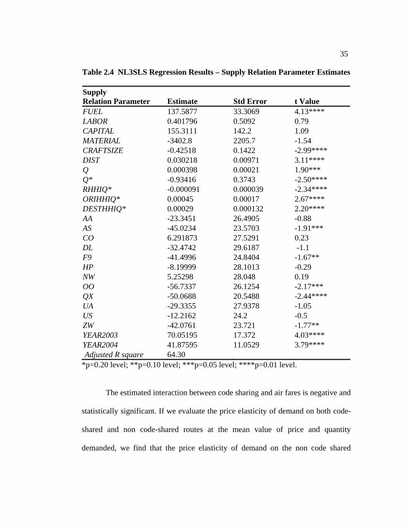
Table 2.4 NL3SLS Regression Results – Supply Relation Parameter Estimates
Supply Relation Parameter Estimate Std Error t Value FUEL 137.5877 33.3069 4.13**** LABOR 0.401796 0.5092 0.79 CAPITAL 155.3111 142.2 1.09 MATERIAL -3402.8 2205.7 -1.54 CRAFTSIZE -0.42518 0.1422 -2.99**** DIST 0.030218 0.00971 3.11**** Q 0.000398 0.00021 1.90*** Q* -0.93416 0.3743 -2.50**** RHHIQ* -0.000091 0.000039 -2.34**** ORIHHIQ* 0.00045 0.00017 2.67**** DESTHHIQ* 0.00029 0.000132 2.20**** AA -23.3451 26.4905 -0.88 AS -45.0234 23.5703 -1.91*** CO 6.291873 27.5291 0.23 DL -32.4742 29.6187 -1.1 F9 -41.4996 24.8404 -1.67** HP -8.19999 28.1013 -0.29 NW 5.25298 28.048 0.19 OO -56.7337 26.1254 -2.17*** QX -50.0688 20.5488 -2.44**** UA -29.3355 27.9378 -1.05 US -12.2162 24.2 -0.5 ZW -42.0761 23.721 -1.77** YEAR2003 70.05195 17.372 4.03**** YEAR2004 41.87595 11.0529 3.79**** Adjusted R square 64.30 *p=0.20 level; **p=0.10 level; ***p=0.05 level; ****p=0.01 level.
The estimated interaction between code sharing and air fares is negative and
statistically significant. If we evaluate the price elasticity of demand on both code-
shared and non code-shared routes at the mean value of price and quantity
demanded, we find that the price elasticity of demand on the non code shared
36
routes is 1.25 while on the code shared routes, it is 5.50. This suggests that code
sharing makes passengers more responsive to the incumbent firms’ price changes.
The population and per capita income in the origin airport MSAs has a
significant impact on demand, but population and per capita income in the
destination airport MSAs has no significant impact. Estimates of most route and
airline dummies are strongly significant, suggesting that unobserved route specific
fixed effects are important as are unobserved airline fixed effects.
VI.2. Supply Relation
The coefficient of is positive ijtQ 8χ =0.000398 and statistically significant,
which means that the increase in marginal cost associated with more landing and
take-offs due to more frequent departures is greater than the cost of carrying one
more additional passenger. Airport dominance, measured by HHI, is a significant
and important source of market power. This result is consistent with previous
studies by Bailey and Williams (1988), Borenstein (1989, 1990, 1991), Berry (1990,
1992), Evans and Kessides (1993), Brueckner and Spiller (1994) and Oum, Zhang
and Zhang (1995). However, high route concentration level tends to decrease
market power, which shows that the threat from potential entry is strong enough to
discourage incumbent airlines to charge monopoly price.
According to our theoretical model, the market power parameter is
1λ ν= + =0.14906 (We get this by substituting the mean values of all the
explanatory variables back into the equation (2.10)). Therefore, v = -0.85094,
37
showing that in the domestic airline market, firms are closer to Bertrand price-
setting than the Cournot quantity-setting competition. This suggests that the nature
of competition in domestic markets tends to be more competitive than in
international markets (Oum, Park and Zhang (1996) and Park and Zhang (2000))
and also more competitive than in domestic airline markets in the 1980s (Brander
and Zhang (1990, 1993)). This result also supports the Bertrand assumption made
by Gayle (2006) in his research on domestic code-sharing alliances.
The signs of three input prices, fuel, labor, capital in the supply relation are
positively related to the price as expected, with the estimates of fuel prices strongly
significant at 1% level of confidence. Estimates of labor, material and capital input
prices are not significant.
Distance tends to increase air fares and aircraft body size is strongly
significant with the expected negative sign, indicating lower marginal costs, a result
consistent with previous studies such as Gillen, Oum and Tretheway (1990),
Capital and Sickles (1997), Fischer and Kamerschen (2003) and Morrison (2006).
Coefficients for airline dummies including AS (Alaska Airlines), F9
(Frontier Airlines), OO (Trans State Airlines), QX (Horizon Air) and ZW (Air
Wisconsin) are significant with the expected negative signs. We expect marginal
cost and thus air fares for these air carriers to be lower because all of these firms
are well-known low cost carriers. Coefficients for two year dummies are significant
as well, which captures the cost changes from 2003 to 2005 due to the dramatic
increase in the world oil prices.
38
VI.3. Incumbent Air Fares and Passenger Volumes
Code sharing tends to increase market demand for incumbents’ nonstop
service but also has an effect on the slope of supply relation curve through PQ
⎛ ⎞∂−⎜ ⎟∂⎝ ⎠
.
Specifically, since the slope of the supply curve is equal to 0.000575 in the
presence of code sharing and increases to 0.000876 in the absence of code sharing,
we expect an increase in equilibrium passenger volumes but are uncertain of the
change in equilibrium air fares. In order to measure the exact changes before and
after Southwest/ATA code sharing on both code-shared and non code-shared routes,
we follow Oum, Park and Zhang (1996) and Park and Zhang (2000) and derive
reduced-form equations for the incumbents’ price and passenger volumes from
equation (2.8) and (2.11):
Q AP B= + and P CQ D= +
where 2 3 itA CSβ β= + ;
0 1 4 5 6 71 1 2
8 91 1 1
;
it it it it itN M
ijt it ijt j j i i t tj i t
ijt
B CS ORIPOP ORIINCO DESTPOP DESTINCO
FREQ CS FREQ FIRM ROUTE YEAR
α β β β β β
β β γ λ ϕ
ϖ
− −
= = =
= + + + + +
+ + + + +
+
∑ ∑ ∑
(If .) '0, then CS B B= =
8 82 3 it
CCS A
λ λχ χβ β
= − = −+
;
and
39
1'
2 3 4 5 6 91
1 2' '
1 1
NF L K M
ijt ijt jt jt ijt i j jj
M
i i t t ijti t
D W W W W CRAFTSIZE DIST FIRM
ROUTE YEAR
χ χ χ χ χ χ γ
λ ϕ δ
−
=
−
= =
= + + + + + +
+ + +
∑
∑ ∑
Therefore, on code-shared routes, where 1CS = , equilibrium air fares and
passenger volumes are 8 2 3 2 3
8 2 3 2 3
( ( ) ) ( )(1 ( ))( )cs
B DP χ β β λ β βλ χ β β β β+ − + +
=+ − + +
and
2 3( )cs csQ P Bβ β= + + . On non code-shared routes, where , equilibrium
passenger volumes and air fares are
0CS =
' '2 8 2
8 2 2
( )(1 )ncs
B DP β χ λ βλ χ β β− +
=+ −
and
. If we substitute the coefficient estimates back into the
expressions above and calculate the air fare and passenger volume for each route
and each year and then take the average of these numbers, we have
and
'2ncs ncsQ Pβ= + B
117009 23071= 93938cs ncsQ Q QΔ = − = − 119 179 = 60cs ncsP P PΔ = − = − − ,
indicating increase in passenger volumes and decrease in air fares.
These results show that code sharing between Southwest and ATA
decreases incumbents’ equilibrium air fares by $60 and increases passenger
volumes by 93938 persons. The decrease in the incumbents’ air fares is consistent
with previous studies documenting the well-known “Southwest Effect”, which
occurs when Southwest directly enters a market. This result suggests that the
“Southwest Effect” is also seen when the carrier enters through code sharing rather
than direct entry. Lower air fares and higher passenger volumes due to code sharing
are also consistent with all previous studies for both international and domestic
40
code sharing (Oum, Park and Zhang (1996), Park (1997), Park and Zhang (2000),
Park, Zhang and Zhang (2001), Park, Park and Zhang (2003), Brueckner and
Whalen (2000), Brueckner (2001, 2003), Bamberger, Carlton and Neumann (2004)
and Armantier and Richard (2005a)).
VI.4. Welfare Analysis of Code sharing
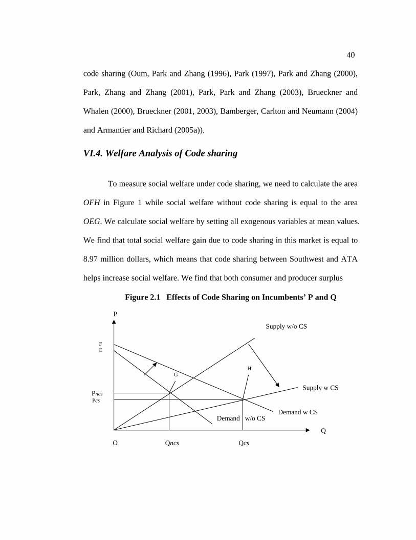
To measure social welfare under code sharing, we need to calculate the area
OFH in Figure 1 while social welfare without code sharing is equal to the area
OEG. We calculate social welfare by setting all exogenous variables at mean values.
We find that total social welfare gain due to code sharing in this market is equal to
8.97 million dollars, which means that code sharing between Southwest and ATA
helps increase social welfare. We find that both consumer and producer surplus
P
Supply w/o CS
Demand w/o CSDemand w CS
Q
O Qncs Qcs
F E
Pncs Pcs
H G
Supply w CS
Figure 2.1 Effects of Code Sharing on Incumbents’ P and Q
41
gains ( million and 4.90CGΔ = 4.07PGΔ = million), a result supported by Park
(1997), Park and Zhang (2000) but contrary to Armantier and Richard (2005b) who
found that consumer welfare decreased after complementary code sharing between
Continental and Northwest Airlines in the US markets. Possible reasons for this
difference could be due to the nature of two code sharing alliances: Continental and
Northwest Airlines are two major legacy air carriers but Southwest and ATA
Airlines are two well-known low cost air carriers. Different business practice
models between low cost and legacy carriers may bring about different effects of
code-sharing alliances.
VII. Conclusions and Future Research
Our empirical results show that the code sharing agreement between
Southwest and ATA in the Denver market increases both producer and consumer
surplus, a finding consistent with studies of international code sharing (Park (1997),
Park and Zhang (2000)) but contrary to Armantier and Richard (2005b) in domestic
markets. We find that this complementary code sharing arrangement decreases
incumbent carriers’ air fares and increases their passenger volumes. Furthermore,
we also find that the domestic airline market structure is more competitive with
competition on price, as opposed to quantity competition in international markets
(Oum, Park and Zhang (1996) and Park and Zhang (2000)) and in domestic
markets in the 1980s (Brander and Zhang (1990, 1993)). This difference may be
due to the fact that our study focuses on domestic code-shared routes where 90% of
42
the passenger volume comes from direct flight services whereas international code-
shared markets are mainly interline markets prior to code sharing. Also,
international markets tend to have fewer carriers and often have regulatory
restrictions that prevent the degree of competition observed in the domestic markets.
Our results provide preliminary evidence that the “Southwest Effect” prevails even
when Southwest entry occurs through code sharing rather than direct entry.
43
References:
Armantier, O. and Richard, O. (2005a), “Evidence on Pricing from the Continental Airlines and Northwest Airlines Code-Share Agreement", Advances in Airline Economics V1, 2006. Elsevier Publisher, edited by Darin Lee; ------(2005b), “Domestic Airline Alliances and Consumer Welfare”, Working papers, University of Montreal, Canada; Bamberger, G.E., Carlton, D.W. and L.R. Neumann (April 2004), “An Empirical Investigation of the Competitive Effects of Domestic Airline Alliances”, Journal of Law and Economics, V XLVII, 195-222; Bennet, R. and Craun, J. (1993), “The Airline Deregulation Evolution Continues: The Southwest Effect”, Office of Aviation Analysis, U.S. Department of Transportation, Washington, D.C.; Boguslaski, C., Ito, H. and Lee, D. (2004), “Entry Patterns in the Southwest Airlines Route System”, Review of Industrial Organization, V24, 317-350; Borenstein, S. (1989), “Hubs and High Fares: Dominance and Market Power in the U.S. Airline Industry”, Rand Journal of Economics, V20(3), 344-365; Borenstein, S and Netz, J. (1999), “Why do all the flights leave at 8 am: Competition and Departure-time Differentiation in the Airline Markets”, International Journal of Industrial Organization, V17(5), 611-640; Brander, J.A. and Zhang, A. (Winter 1990), “Market Conduct in the Airline Industry: An Empirical Investigation,” Rand Journal of Economics, V21(4), 217-233; -------- (1993), “Dynamic Oligopoly Behavior in the Airline Industry,” International Journal of Industrial Organization, V11, 407-435; Bresnahan, T.F. (1982), “The Oligopoly Solution Concept Is Identified”, Economics Letters, V10, 87-92; --------- (1989), “Empirical Studies of Industries with Market Power”, In R. Schmalensee and R.D. Willing (eds.): Handbook of Industrial Organization, Chapter 7, 1011-1057. New York: North Holland;
Brueckner, J.K. (2001), “The Economics of International Code-sharing: an Analysis of Airline Alliances,” International Journal of Industrial Organization, V19, 1475-1498;
44
------- (2003), “International Airfares in the Age of Alliances: The Effects to Code-sharing and Antitrust Immunity”, Review of Economic Statistics, V85, 105-118; Brueckner, J.K. and Spiller, P.T. (October 1994), “Economies of Traffic Density in the Deregulated Airline Industry”, Journal of Law and Economics, V37(2), 379-415; Brueckner, J.K. and Whalen, W.T. (October 2000), “The Price Effect of International Airline Alliances”, Journal of Law and Economics, V XLIII, 503-544; Captain, P.F. and Sickles, R.C. (1997), “Competition and Market Power in the European Airline Industry: 1976-90”, Managerial and Decision Economics, V18, 209-225; Caves, R.E. (1962), Air Transport and Its Regulators, Cambridge, MA, Harvard University Press; Caves, D.W., Christensen, L.R. and Tretheway, M.W. (1984), “Economies of Density versus Economies of Scale: Why Trunk and Local Service Airline Costs Differ”, Rand Journal of Economics, V15, 471-489; Chua, C.L., Kew, H and Yong, J (2005), “Airline Code-sharing Alliances and Costs: Imposing Concavity on Translog Cost Function Estimation”, Review of Industrial Organization V26, 461-487; Creel, M. and Farell, M. (2001), “Economies of Scale in the US Airline Industry after Deregulation: A Fourier Series Approximation”, Transportation Research Part E, V37, 321-336; Douglas, G.W. and Miller III, J.C. (1974), Economic Regulation of Domestic Air Transport: Theory and Policy, Washington, D.C., Brookings Institution; Eads, G.C., Nerlove, M. and Raduchel, W. (August 1969), “A Long-run Cost Function for the Local Service Airline Industry”, Review of Economics and Statistics, V51, 258-270; Fischer, T. and Kamerschen, D.R. (May 2003), “Price-Cost Margins in the US Airline Industry using a Conjectural Variation Approach”, Journal of Transport Economics and Policy, V 37(2), 227-259; Fu, X., Dresner, M. and Oum, T.H. (2006), “Oligopoly Competition with Differentiated Products: What Happened After the Effect of Southwest’s Entries Stabilized”, Unpublished Working paper, Sauder School of Business, University of British Columbia, Vancouver, Canada;
45
Gayle, P.G. (2006), “Airline Code-share Alliances and Their Competitive Effects”, Journal of Law and Economics, forthcoming; Gillen, D.W., Oum, T.H. and Tretheway, M.W. (1990), “Airline Cost Structure and Policy Implications”, Journal of Transport Economics and Policy, V24, 9-34; Green, W.H. (2003), Econometric Analysis, Fifth edition, Prentice Hall; Hassin, O. and Shy, O. (2004), “Code-sharing Agreements and Interconnections in Markets for International Flights”, Review of International Economics, V12(3), 337-352; Iwata, G. (1974), “Measurement of Conjectural Variations in Oligopoly”, Econometrica, V42, 947-966; Keeler, T.E. (1978), “Domestic Trunk Airline Regulation: An Economic Evaluation”, Study on Federal Regulation, Washington, D.C., US Government Printing Office Morrison, S.A. (2001), “Actual, Adjacent and Potential Competition: Estimating the Full Effect of Southwest Airlines”, Journal of Transport Economics and Policy, V35, 239-256; ------(2006), “Airline Service: The Evolution of Competition Since Deregulation”, Industry and Firm Studies, NY: M.E. Sharpe, Inc., forthcoming 2007, edited by Victor J. Tremblay and Carol Tremblay; Morrison, S.A. and Winston, C. (1995), The Evolution of the Airline Industry, The Brookings Institution, Washington, DC; Oum, T.H., Park, J.H. and Zhang, A. (1996), “The Effects of Airline Code-sharing Agreements on Firm Conduct and International Air Fares”, Journal of Transport Economics and Policy, V30(2), 187-202; Oum, T.H. and Yu, C. (1998), Winning Airlines: Productivity and Cost Competitiveness of the World’s Major Airlines, Boston, Kluwer Academic Publishers, 1998; Oum, T.H., Zhang, A. and Zhang Y. (1993), “Inter-firm Rivalry and Firm-specific Price Elasticties in Deregulated Airline Markets”, Journal of Transport Economics and Policy, V27(2), 171-192;
46
Oum, T.H. and Zhang, Y. (1991), “Utilization of Quasi-Fixed Inputs and Estimation of Cost Functions”, Journal of Transport Economics and Policy, V25, 121-135; Park, J. (1997), “The Effects of Airline Alliances on Markets and Economic Welfare”, Transportation Research Part E: Logistics and Transportation Review, V33(3), 181-195; Park, J.H., Park, N.K. and Zhang, A. (2003), “The Impact of International Alliances on Rival Firm Value: A Study of the British Airways US Air Alliance”, Transportation Research Part E: Logistics and Transportation Review, V39(1), 1-18; Park, J. and Zhang A. (2000), “An Empirical Analysis of Global Airline Alliances: Cases in North Atlantic Markets”, Review of Industrial Organization, V16: 367-383; Park, J.H., Zhang, A. and Zhang, Y. (2001), “Analytical Models of International Alliances in the Airline Industry”, Transportation Research Part B: Methodological, V35(9), 865-886; Shy, O. (2001), The Economics of Network Industries, Cambridge University Press; United States General Accounting Office (June 4, 1998), “Aviation Competition---Proposed Domestic Airline Alliances Raise Serious Issues”.
47
Chapter 3
Determinants of Successful Code-sharing: A Case Study of Continental and America West Airlines Alliances --- A Discrete
Longitudinal Analysis
48
I. Introduction
Six major domestic U.S. airlines (Delta and United Airlines, American and
US Airways, Northwest and Continental Airlines) proposed various kinds of
alliances in 1998. All of these alliances combined frequent flier programs and club
facilities. Northwest Airlines planned to buy an equity share in Continental Airlines.
Delta and United and Northwest and Continental entered into code-sharing
agreements.
Code-sharing has emerged as one of the most important forms of alliance in
the airline industry. Under code-sharing, contracting firms merge their
computerized reservation systems so that each contracting carrier can issue tickets
with their own flight numbers on flights operated by other contracting air carriers.
Through code-sharing, partner firms effectively link their networks without
operating additional aircraft and gain exposure in markets where they do not
operate directly but participate via display of their flight numbers. As a result,
airlines are able to make use of hub-and-spoke systems to generate greater
passenger volumes. Due to economies of traffic density, the marginal operating
cost of carrying an additional passenger drops with increased volume, explaining
why code-sharing has become a popular form of airline alliance.
The first major code-sharing alliance in the US airline industry began in the
middle of the 1990s between Continental and America West Airlines. America
West Airlines, the second largest low cost air carrier in the US, now operating as
US Airways, was one of the greatest business successes in the US airline industry
49
in the 1980s. But rapid expansion growth without proper handling of large
operating losses placed the company at the verge of bankruptcy by 1986. With the
pressure from increasing fuel costs due to concerns about stability in the Gulf
States in the lead-up to the Persian Gulf War, America West was forced to file for
bankruptcy in 1991. In 1994, America West managed to secure reorganization,
with a large portion of the airline owned by a partnership with Continental Airlines.
This partnership resulted in a code-sharing arrangement with Continental and
heralded the beginning of code-sharing alliances in the domestic airline industry.
The America West and Continental code-sharing arrangement lasted 8 years,
from 1994 to 2002.17 During the code-sharing period, individual routes were added
and old routes dropped. Indeed, the route structure of the code-share agreement was
very dynamic as indicated in Table 3.1. The purpose of this paper is to examine
why some routes were kept and others deleted.
Previous studies have examined the effect of code-sharing on air fares,
passenger volumes, operating costs and consumer welfare (Oum, Park and Zhang
(1996), Park (1997), Park and Zhang (2000), Park, Zhang and Zhang (2001), Park,
Park and Zhang (2003), Brueckner and Whalen (2000), Shy (2001), Brueckner
17 Continental Airlines, the fourth largest US airline with headquarters in Houston, Texas and operations throughout the US, Canada, Latin America, Europe and the Asia-Pacific region, has entered a number of subsequent alliances. As of 2007, it had more than 3,000 daily departures, serving 151 domestic and 120 international destinations and has 42,200 employees. In September 2004, Continental became a member of the SkyTeam Alliance, in which it participates with Delta Air Lines, Northwest Airlines and KLM Royal Dutch Airlines. It also initiated code-sharing with Amtrak rail services to some cities in the northeastern United States, which is the first code-sharing agreement between airline and rail services.
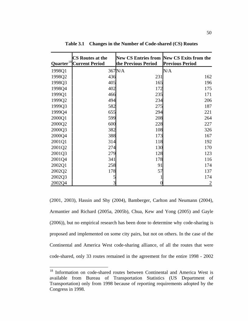
50
Table 3.1 Changes in the Number of Code-shared (CS) Routes
Quarter18CS Routes at the Current Period
New CS Entries from the Previous Period
New CS Exits from the Previous Period
1998Q1 367 N/A N/A 1998Q2 436 231 1621998Q3 405 165 1961998Q4 402 172 1751999Q1 466 235 1711999Q2 494 234 2061999Q3 582 275 1871999Q4 655 294 2212000Q1 599 208 2642000Q2 600 228 2272000Q3 382 108 3262000Q4 388 173 1672001Q1 314 118 1922001Q2 274 130 1702001Q3 279 128 1232001Q4 341 178 1162002Q1 258 91 1742002Q2 178 57 1372002Q3 5 1 1742002Q4 3 0 2
(2001, 2003), Hassin and Shy (2004), Bamberger, Carlton and Neumann (2004),
Armantier and Richard (2005a, 2005b), Chua, Kew and Yong (2005) and Gayle
(2006)), but no empirical research has been done to determine why code-sharing is
proposed and implemented on some city pairs, but not on others. In the case of the
Continental and America West code-sharing alliance, of all the routes that were
code-shared, only 33 routes remained in the agreement for the entire 1998 - 2002
18 Information on code-shared routes between Continental and America West is available from Bureau of Transportation Statistics (US Department of Transportation) only from 1998 because of reporting requirements adopted by the Congress in 1998.
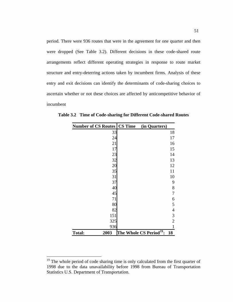
51
period. There were 936 routes that were in the agreement for one quarter and then
were dropped (See Table 3.2). Different decisions in these code-shared route
arrangements reflect different operating strategies in response to route market
structure and entry-deterring actions taken by incumbent firms. Analysis of these
entry and exit decisions can identify the determinants of code-sharing choices to
ascertain whether or not these choices are affected by anticompetitive behavior of
incumbent
Table 3.2 Time of Code-sharing for Different Code-shared Routes
Number of CS Routes CS Time (in Quarters) 33 18 24 17 21 16 17 15 23 14 32 13 20 12 35 11 31 10 37 9 40 8 45 7 71 6 80 5 82 4
151 3 325 2 936 1
Total: 2003 The Whole CS Period19: 18
19 The whole period of code sharing time is only calculated from the first quarter of 1998 due to the data unavailability before 1998 from Bureau of Transportation Statistics U.S. Department of Transportation.
52
firms. For government agents and policy makers, identification of the determinants
of code-sharing can provide information as how to regulate alliances and predict
that which specific factors should be considered when reviewing a proposed code-
share agreement. The results from this study should help policy makers determine
the extent they should be concerned with antitrust issues when considering
approval of a new agreement. For individual firms considering which routes to
include in a code-share agreement, this study provides information on which are the
relevant factors to consider.
II. Literature Review
The importance of entry conditions and their impact on economic
performance in the process of competition has long been of concern in the
industrial organization literature. Extra-normal or excess economic profits in an
industry suggest that entry barriers may exist to keep other firms from entering and
taking advantage of the market profitability. Bain’s (1956) pioneering work points
out that economies of scale, absolute cost and product differentiation advantages of
incumbent firms are three elements that affect the ability of incumbent firms to
protect positive profits from entry.
However, the nature of Bain’s paradigm is entirely static with entry barriers
taken as exogenous, problems which have been addressed in the game-theoretic
literature. Sutton (1991) provides a two-stage game formulation and offers a
detailed study of the role sunk costs play, either endogenously or exogenously, as
53
entry barriers.20 In the airline literature, the most noteworthy work regarding entry
conditions has been the theory of contestable markets. Bailey and Panzar (1981)
argued that long haul airline markets served by local service monopolists were
basically contestable. Baumol (1982) formally defined a perfectly contestable
market as a market with freedom of entry and exit without incurring loss of sunk
cost. Perfect contestability guarantees absence of excess profits and cross
subsidization even under monopoly or oligopoly situations. Bailey and Baumol
(1984) further point out that even though airline markets could theoretically be
represented as contestable, labor contracts, slot controls, airport dominance and
long-term lease of airport facilities all may prevent contestability from occurring.21
This conclusion is consistent with Morrison and Winston (1987), Hurdle et al.
(1989), Strassmann (1990) and Winston and Collins (1992) who agree that perfect
contestability did not characterize the airline industry after deregulation. In
particular, Morrison and Winston (1987), Sinclair (1995), Dresner, Lin and Windle
(1996), Morrison (2001), Dresner, Windle and Yao (2002) find that slot controls
were a significant entry deterrent.
Bailey and William (1988), Borenstein (1989, 1990, 1991), Berry (1990,
1992), Evans and Kessides (1993) and Oum, Zhang and Zhang (1995) argue that
20 For a detailed review of empirical studies of entry and exit, please refer to Siegfried and Evans (1994). 21 Since 1968, four airports in the U.S. have limits on the number of takeoffs and landings that may take place during any given hour. They are Chicago O’ Hare, New York Kennedy and La Guardia and Washington Reagan National Airports. But in 1986, the U.S. Department of Transportation permitted airlines to buy and sell their takeoff and landing slots.
54
airport dominance (hub concentration) is an important source of market power and
monopoly rents, representing a dominant strategy in the oligopolistic deregulated
airline industry. From the demand side, a dominant reputation can be acquired by a
scale-driven carrier as a consequence of operating most flights at its hub airport,
raising the value of the airline’s frequent flyer program and creating brand loyalty.
Large scale operations by an incumbent carrier can result in higher flight
frequency------an important indicator of service quality, and may also inhibit
potential competitors’ abilities to obtain gates and other facilities necessary for
entry or expansion of service. From the cost side, increased flight frequency may
increase traffic density, which leads to lower marginal operating cost and generates
cost advantages over potential entrants if the increase in costs associated with an
increase in flight frequency is less than revenues produced by the additional
passengers. 22 From both demand and cost sides, economies of density play an
important role in creating entry barriers.
Travel agent commission override bonuses and biases due to computer
reservation systems may benefit incumbent carriers; long-term leases of airport
space to particular carriers give them the power to decide when, to whom and at
what price to sublease space to competitors.
High route concentration may also be a significant deterrent to entry in the
airline industry. Hurdle etc. (1989) and Strassmann (1990) find that entry barriers
22 Please see also Caves, Christensen and Tretheway (1984), Brueckner, Dyer and Spiller (1992), Brueckner and Spiller (1994) and Hendricks, Piccione and Tan (1995) for details of economies of aircraft size and economies of traffic density as an important reason of adopting hub-and-spoke systems.
55
exist in the highly concentrated airline markets due to incumbents’ large scale
flight operations at their hub airports.
With the formation of hub-and-spoke networks after deregulation, airport
congestion has become an important entry barrier to potential entrants. Abramowitz
and Brown (1993) and Dresner, Windle and Yao (2002) find that airport congestion
measured either by the number of takeoffs and landings or by gate constraints and
utilization are significant barriers to entry.
Finally, what is worth mentioning is that perfect contestability theory
assumes that all players in the market have the same cost structure so the entrants
can serve the market demands with the same technology by engaging in “hit-and-
run” entry without incurring sunk cost. But this is not true in the airline industry.
Low cost air carriers usually enjoy a cost advantage and can earn profits at prices
that are not compensatory to incumbent carriers. Low cost carriers are able to do
this because they use a different business model than legacy carrier, such as only
operating a single type of airplane, servicing a single passenger class, managing a
simple fare scheme, and flying to cheaper, less congested secondary airports to
avoid air traffic delays and take advantage of lower landing fees. Whinston and
Collins (1992) provide an example of the successful entry of a low cost air carrier
People Express, which led to significant value reductions for incumbent firms.
Bennett and Craun (1993), Windle and Dresner (1995), Dresner, Lin and Windle
(1996), Richards (1996), Morrison (2001), Bamberger and Carlton (2006) all find
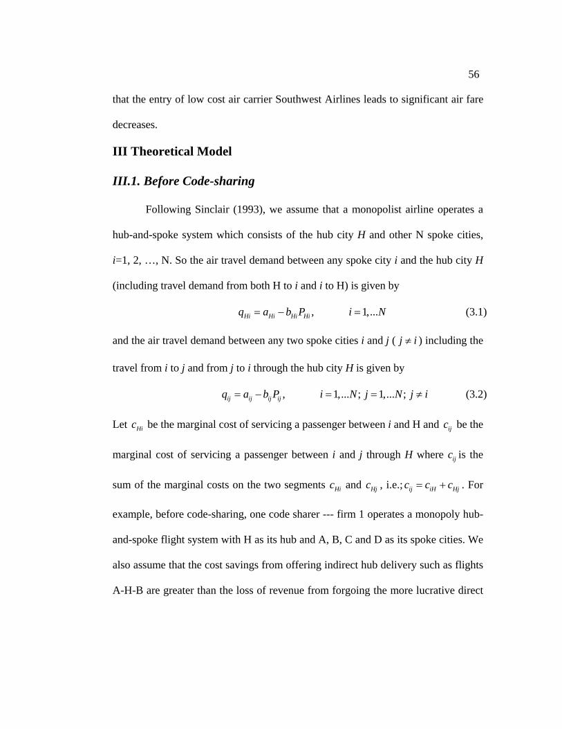
56
that the entry of low cost air carrier Southwest Airlines leads to significant air fare
decreases.
III Theoretical Model
III.1. Before Code-sharing
Following Sinclair (1993), we assume that a monopolist airline operates a
hub-and-spoke system which consists of the hub city H and other N spoke cities,
i=1, 2, …, N. So the air travel demand between any spoke city i and the hub city H
(including travel demand from both H to i and i to H) is given by
, 1,... Hi Hi Hi Hiq a b P i N= − = (3.1)
and the air travel demand between any two spoke cities i and j ( j i≠ ) including the
travel from i to j and from j to i through the hub city H is given by
, 1,... ; 1,... ; ij ij ij ijq a b P i N j N j i= − = = ≠ (3.2)
Let Hic be the marginal cost of servicing a passenger between i and H and be the
marginal cost of servicing a passenger between i and j through H where is the
sum of the marginal costs on the two segments
ijc
ijc
Hic and Hjc , i.e.; . For
example, before code-sharing, one code sharer --- firm 1 operates a monopoly hub-
and-spoke flight system with H as its hub and A, B, C and D as its spoke cities. We
also assume that the cost savings from offering indirect hub delivery such as flights
A-H-B are greater than the loss of revenue from forgoing the more lucrative direct
ij iH Hjc c c= +
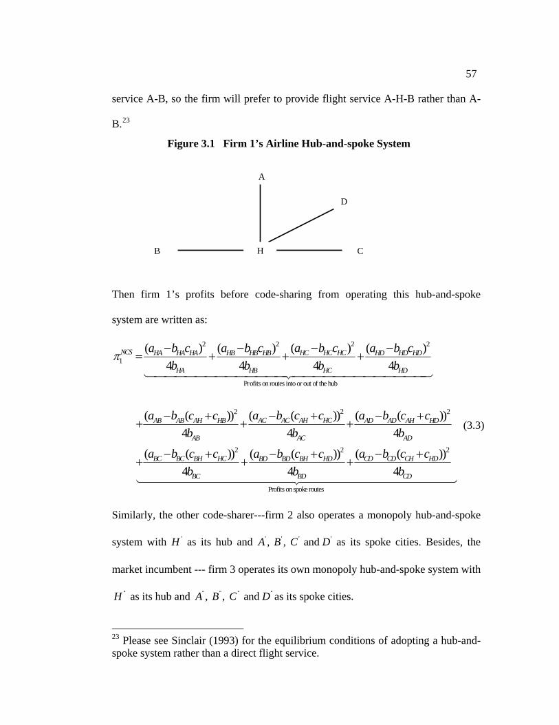
57
service A-B, so the firm will prefer to provide flight service A-H-B rather than A-
B.23
Figure 3.1 Firm 1’s Airline Hub-and-spoke System
A
D
HB C
Then firm 1’s profits before code-sharing from operating this hub-and-spoke
system are written as:
22 2
1
Profits on routes into or out of the hub
( )( ) ( ) ( )4 4 4 4
NCS HC HC HCHA HA HA HB HB HB HD HD HD
HA HB HC HD
a b ca b c a b c a b cb b b b
π −− − −= + + +
2
22 2
2 22
Profits on spoke rou
( ( ))( ( )) ( ( ))4 4 4
( ( )) ( ( ))( ( ))
4 4 4
AC AC AH HCAB AB AH HB AD AD AH HD
AB AC AD
BC BC BH HC CD CD CH HDBD BD BH HD
BC BD CD
a b c ca b c c a b c cb b b
a b c c a b c ca b c cb b b
− +− + − ++ + +
− + − +− ++ + +
tes
(3.3)
Similarly, the other code-sharer---firm 2 also operates a monopoly hub-and-spoke
system with H as its hub and 'A B as its spoke cities. Besides, the
market incumbent --- firm 3 operates its own monopoly hub-and-spoke system with
as its hub and as its spoke cities.
' ' ' ', , and C D
''H '' '' '' '', , and A B C D
23 Please see Sinclair (1993) for the equilibrium conditions of adopting a hub-and-spoke system rather than a direct flight service.
58
III.2. After Code-sharing
Under code-sharing, firm 1 (firm 2) chooses several spoke cities in its own
hub-and-spoke system as the connecting airport cities and constitutes the
complementary code-shared routes with firm 2 (firm 1). We limit our attention to
one-stop (two segments) complementary code-shared flights only, so there are
actually three airport cities involved --- the origin airport, the connecting airport
and the destination airport. Every airport acts as either the hub or the spoke city in
the code-sharing. If we assume alliance firms are symmetric, then there are totally
eight ways of setting up code-sharing ------ Hub-Hub-Hub, Hub-Hub-Spoke, Hub-
Spoke-Hub, Hub-Spoke-Spoke, Spoke-Hub-Hub, Spoke-Hub-Spoke, Spoke-
Spoke-Hub and Spoke-Spoke-Spoke. If a city is the hub city for one firm but a
spoke city for another firm, we regard this city as a hub city. For example, H-C-H’
and H-D-H’ are two “Hub-Spoke-Hub” kind of code-shared routes. To keep the
model as succinct as possible without losing any generality, the theoretical model
and profit function specified in the paper is based on Hub-Spoke-Hub code-sharing
route arrangement. However, the profit function from other code-sharing route
arrangements can be specified similarly without changing the essence of
equilibrium conditions derived from the paper. Please refer to Figure A1 for details.
In Figure 3.2, both city C (C’) and D (D’) are the spoke cities in firm 1 and 2’s hub-
and-spoke systems respectively. Before code-sharing, neither of the firms provides
services on the trip with city H as the origin and city H’ as the destination but the
market incumbent---firm 3 provides one-stop flights A”(H)-H”-B”(H’)
59
A A’
through its own hub H” and enjoys the monopoly profits. Under code-sharing,
alliance firms choose their spoke cities such as C (C’) and D(D’) as the connecting
airport cities and provide code-shared flights H-C-H’ and (or) H-D-H’ on the trip
with city H as the origin and city H’ as the destination. Therefore, through code-
sharing, firm 1 and firm 2, acting as one firm, enter route HH’ and compete with
the one-stop flights offered by the market incumbent---firm 3. Due to economies of
traffic density, the increased passenger volumes from code-shared flights will
decrease the marginal operating cost on segments HC(H’C’) and HD(H’D’) in both
firm 1 and firm 2’s hub-and-spoke system, assuming all other things stay the same.
Let Hic be the marginal cost on the segment Hi after code-sharing where Hic
satisfies Hi Hic c< --- the marginal cost on the segment Hi before code-sharing. The
H (A”) B C (C’)
D (D’)
B’H’(B”)
H”
Figure 3.2 Code-sharing Alliances under Airlines’ Hub-and-spoke Flight Systems
C” D”
60
decrease in marginal costs on the segments HC and HD also helps decrease the
marginal cost of flight itineraries that contain either of the two segments such as A-
H-C, B-H-C, A-H-D, B-H-D and C-H-D. For example, the marginal cost of flights
on route A-H-D after code-sharing, denoted by ADc ( AD HAHc c c= + D ),
satisfies AD ADc c< ---the marginal cost on route A-H-D before code-sharing
( AD AH Hc c c= + D ) because HD HDc c< . Accordingly, the marginal operating cost of
firm 2 will decrease by the same way as well.
However, the marginal cost of the market incumbent (firm 3) on segment
HH” and H”H’ will increase because some passengers may choose code-shared
flights offered by firm 1 (or firm 2) instead of one-stop flights offered by firm 3.
Decreased passenger volumes of firm 3 on the segments HH” (A”H”) and H”H’
(H”B”) will increase the marginal cost on these segments and on the flight
itineraries that contain either of these segments. Let 'HHc ( ' " " 'HH HH Hc c c= + H ) be
the incumbent’s marginal cost on the contested route HH’ after code-sharing where
" " '" " ' and HH H HHH Hc c c c> > "H with HHc and " 'H Hc as the incumbent’s marginal cost
on the segment HH” and H”H’ before code-sharing. So ' 'HH HHc c> ,
where ' " " 'HH HH Hc c c= + H . In addition, the incumbent’s marginal cost on flight
itineraries in its hub-and-spoke system that contain the contested segment also
increases. For example, the marginal cost on route H-H”-D” after code-sharing,
denoted by " " " " "( )HD HD HH H Dc c c c= + , satisfies " "HD HDc c> ,
where
" " "( )HD HH H Dc c c= + "
"HDc is the incumbent’s marginal cost on route H-H”-D” before code-
61
sharing. Hence, code-sharing between firm 1 and firm 2 actually affects the
marginal costs of all three firms in their respective hub-and-spoke systems.
We specify the demand and profit functions for firm 1 in its hub-and-spoke
system after code-sharing with firm 2 as follows:
a. The demand and profit functions between the spoke city i and the hub city
H---the segment Hi where Hi is not a code-shared segment are given by
, 1,... Hi Hi Hi Hiq a b P i L= − = (3.4)
and
( ) , 1,...Hi Hi Hi HiP c q i Lπ = − = (3.5)
where Hic is the marginal cost of firm 1 on the non code-shared segment Hi;
b. The demand and profit functions on the segment Hm where Hm is a code-
shared segment are given by
(3.6) , 1,... , Hm Hm Hm Hmq a b P m G G N L= − = = −
and
( ) , < , 1,... , Hm HmHm Hm Hm HmP c q c c m G G N Lπ = − = = − (3.7)
where Hmc is the after-code-sharing marginal cost of firm 1 on the segment
Hm and Hmc is the before-code-sharing marginal cost of firm 1 on the
segment Hm;
c. The demand and profit functions between two spoke cities i and j through
the hub H where i-H-j or j-H-i does not contain code-shared segments are
given by
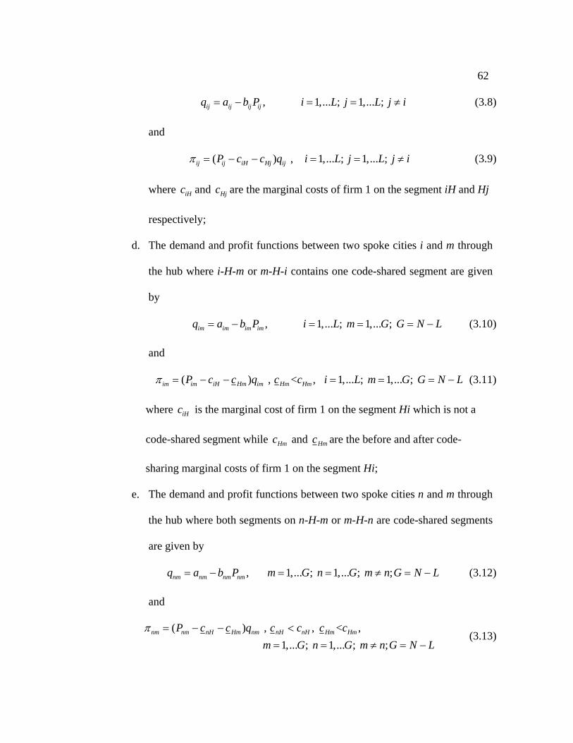
62
(3.8) , 1,... ; 1,... ; ij ij ij ijq a b P i L j L j i= − = = ≠
and
( ) , 1,... ; 1,... ; ij ij iH Hj ijP c c q i L j L j iπ = − − = = ≠ (3.9)
where and iHc Hjc are the marginal costs of firm 1 on the segment iH and Hj
respectively;
d. The demand and profit functions between two spoke cities i and m through
the hub where i-H-m or m-H-i contains one code-shared segment are given
by
(3.10) , 1,... ; 1,... ; im im im imq a b P i L m G G N L= − = = = −
and
( ) , < , 1,... ; 1,... ; Hm Hmim im iH im HmP c c q c c i L m G G N Lπ = − − = = = − (3.11)
where is the marginal cost of firm 1 on the segment Hi which is not a iHc
code-shared segment while Hmc and Hmc are the before and after code-
sharing marginal costs of firm 1 on the segment Hi;
e. The demand and profit functions between two spoke cities n and m through
the hub where both segments on n-H-m or m-H-n are code-shared segments
are given by
(3.12) , 1,... ; 1,... ; ; nm nm nm nmq a b P m G n G m n G N L= − = = ≠ = −
and
( ) , , < ,
1,... ; 1,... ; ;nH Hm nH Hmnm nm nm nH HmP c c q c c c c
m G n G m n G N Lπ = − − <
= = ≠ = − (3.13)
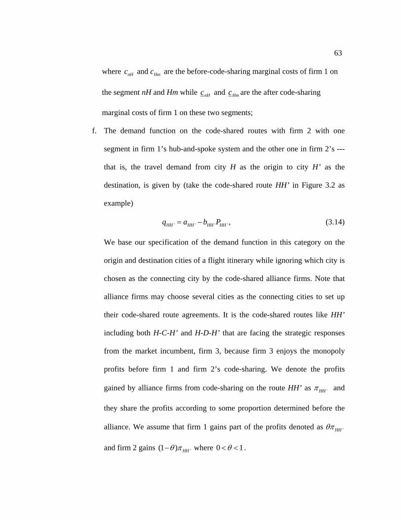
63
where are the before-code-sharing marginal costs of firm 1 on and nH Hmc c
the segment nH and Hm while nHc and Hmc are the after code-sharing
marginal costs of firm 1 on these two segments;
f. The demand function on the code-shared routes with firm 2 with one
segment in firm 1’s hub-and-spoke system and the other one in firm 2’s ---
that is, the travel demand from city H as the origin to city H’ as the
destination, is given by (take the code-shared route HH’ in Figure 3.2 as
example)
' ' ' ' , HH HH HH HHq a b P= − (3.14)
We base our specification of the demand function in this category on the
origin and destination cities of a flight itinerary while ignoring which city is
chosen as the connecting city by the code-shared alliance firms. Note that
alliance firms may choose several cities as the connecting cities to set up
their code-shared route agreements. It is the code-shared routes like HH’
including both H-C-H’ and H-D-H’ that are facing the strategic responses
from the market incumbent, firm 3, because firm 3 enjoys the monopoly
profits before firm 1 and firm 2’s code-sharing. We denote the profits
gained by alliance firms from code-sharing on the route HH’ as 'HHπ and
they share the profits according to some proportion determined before the
alliance. We assume that firm 1 gains part of the profits denoted as 'HHθπ
and firm 2 gains '(1 ) HHθ π− where 0 1θ< < .
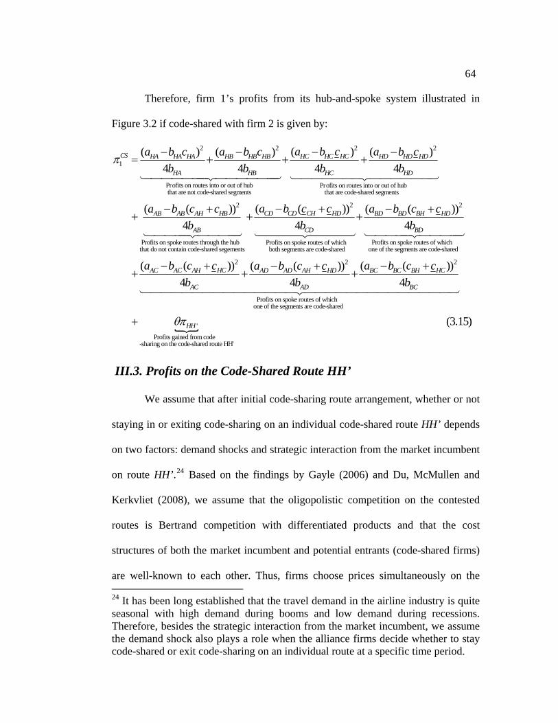
64
Therefore, firm 1’s profits from its hub-and-spoke system illustrated in
Figure 3.2 if code-shared with firm 2 is given by:
22 2 2
1
Profits on routes into or out of hub Profits on routes into or out of hub that are not code-shared segments
( )( ) ( ) ( )4 4 4 4
CS HCHC HC HDHA HA HA HB HB HB HD HD
HA HB HC HD
a b ca b c a b c a b cb b b b
π −− − −= + + +
that are code-shared segments
22
Profits on spoke routes through the hub Profitthat do not contain code-shared segements
( ( ))( ( )) 4 4
CH HDCD CDAB AB AH HB
AB CD
a b c ca b c cb b
− +− ++ +
2
Profits on spoke routes of which s on spoke routes of whichone of the segments are code-shared both segments are code-shared
( ( )4
( ( )
HDBD BD BH
BD
HCAC AC AH
a b c cb
a b c c
− ++
− ++
)
2 22
Profits on spoke routes of which one of the segments are code-shared
' Profits gained from cod
) ( (( ( ))4 4 4
HCHD BC BC BHAD AD AH
AC AD BC
HH
a b c ca b c cb b b
θπ
− +− ++ +
+e
-sharing on the code-shared route HH'
(3.15)
))
III.3. Profits on the Code-Shared Route HH’
We assume that after initial code-sharing route arrangement, whether or not
staying in or exiting code-sharing on an individual code-shared route HH’ depends
on two factors: demand shocks and strategic interaction from the market incumbent
on route HH’.24 Based on the findings by Gayle (2006) and Du, McMullen and
Kerkvliet (2008), we assume that the oligopolistic competition on the contested
routes is Bertrand competition with differentiated products and that the cost
structures of both the market incumbent and potential entrants (code-shared firms)
are well-known to each other. Thus, firms choose prices simultaneously on the
24 It has been long established that the travel demand in the airline industry is quite seasonal with high demand during booms and low demand during recessions. Therefore, besides the strategic interaction from the market incumbent, we assume the demand shock also plays a role when the alliance firms decide whether to stay code-shared or exit code-sharing on an individual route at a specific time period.
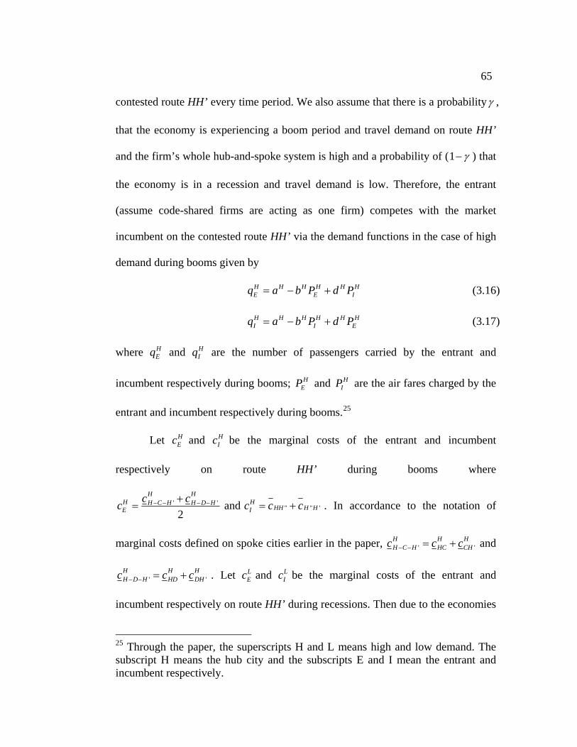
65
contested route HH’ every time period. We also assume that there is a probabilityγ ,
that the economy is experiencing a boom period and travel demand on route HH’
and the firm’s whole hub-and-spoke system is high and a probability of (1 γ− ) that
the economy is in a recession and travel demand is low. Therefore, the entrant
(assume code-shared firms are acting as one firm) competes with the market
incumbent on the contested route HH’ via the demand functions in the case of high
demand during booms given by
H H H H HE Eq a b P d P= − + H
I (3.16)
H H H H HI Iq a b P d P= − + H
E (3.17)
where HEq and H
Iq are the number of passengers carried by the entrant and
incumbent respectively during booms; HEP and H
IP are the air fares charged by the
entrant and incumbent respectively during booms.25
Let HEc and H
Ic be the marginal costs of the entrant and incumbent
respectively on route HH’ during booms where
' '
2
H HH H C H H D HE
c cc − − − −+= and " "
H'HH HIc c c= + H . In accordance to the notation of
marginal costs defined on spoke cities earlier in the paper, ' 'H H HH C H HC CHc c− − = + c and
'H H
'H
H D H HD DHc c c− − = + . Let and be the marginal costs of the entrant and
incumbent respectively on route HH’ during recessions. Then due to the economies
LEc L
Ic
25 Through the paper, the superscripts H and L means high and low demand. The subscript H means the hub city and the subscripts E and I mean the entrant and incumbent respectively.
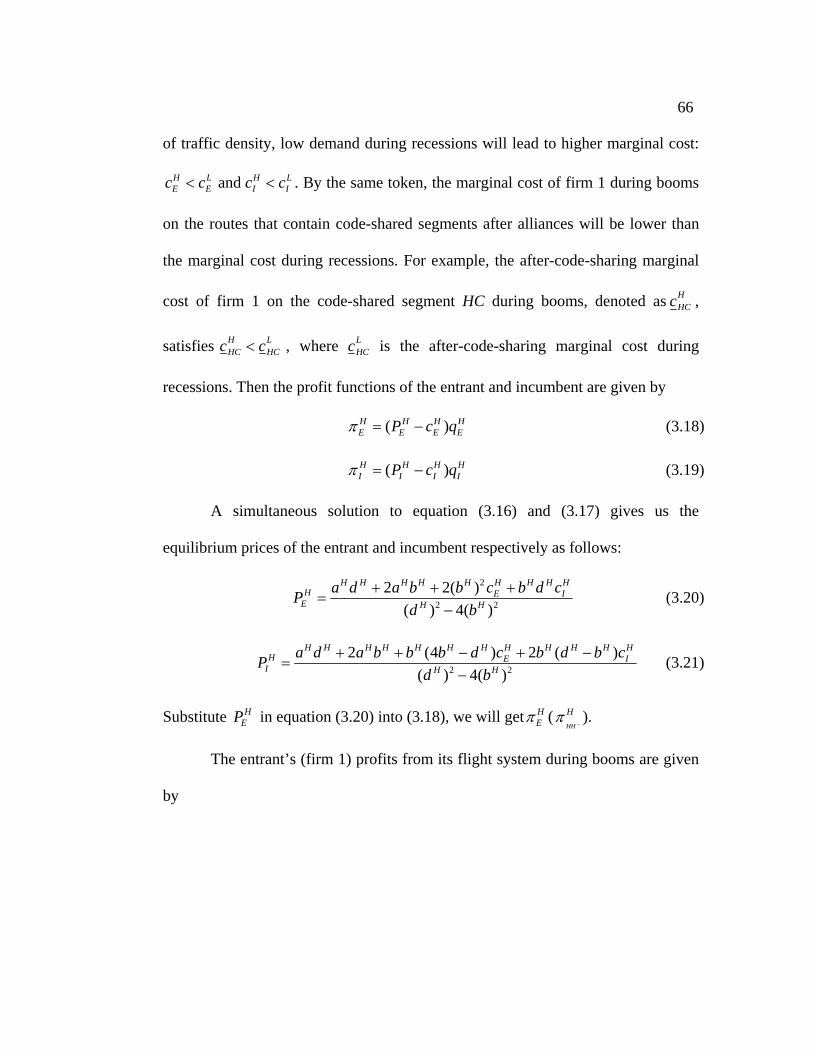
66
of traffic density, low demand during recessions will lead to higher marginal cost:
and H L HE E Ic c c c< L
I< . By the same token, the marginal cost of firm 1 during booms
on the routes that contain code-shared segments after alliances will be lower than
the marginal cost during recessions. For example, the after-code-sharing marginal
cost of firm 1 on the code-shared segment HC during booms, denoted as HHCc ,
satisfies H LHC Hc c< C , where L
HCc is the after-code-sharing marginal cost during
recessions. Then the profit functions of the entrant and incumbent are given by
( ) H H H HE E E EP c qπ = − (3.18)
( ) H H H HI I I IP c qπ = − (3.19)
A simultaneous solution to equation (3.16) and (3.17) gives us the
equilibrium prices of the entrant and incumbent respectively as follows:
2
2 2
2 2( )( ) 4( )
H H H H H H H HH E
E H H
a d a b b c b d cPd b
+ + +=
−
HI (3.20)
2 2
2 (4 ) 2 (( ) 4( )
)H H H H H H H H H H HH E I
I H H
a d a b b b d c b d b cPd b
+ + − + −=
−
H
(3.21)
Substitute HEP in equation (3.20) into (3.18), we will get H
Eπ ('HH
Hπ ).
The entrant’s (firm 1) profits from its flight system during booms are given
by
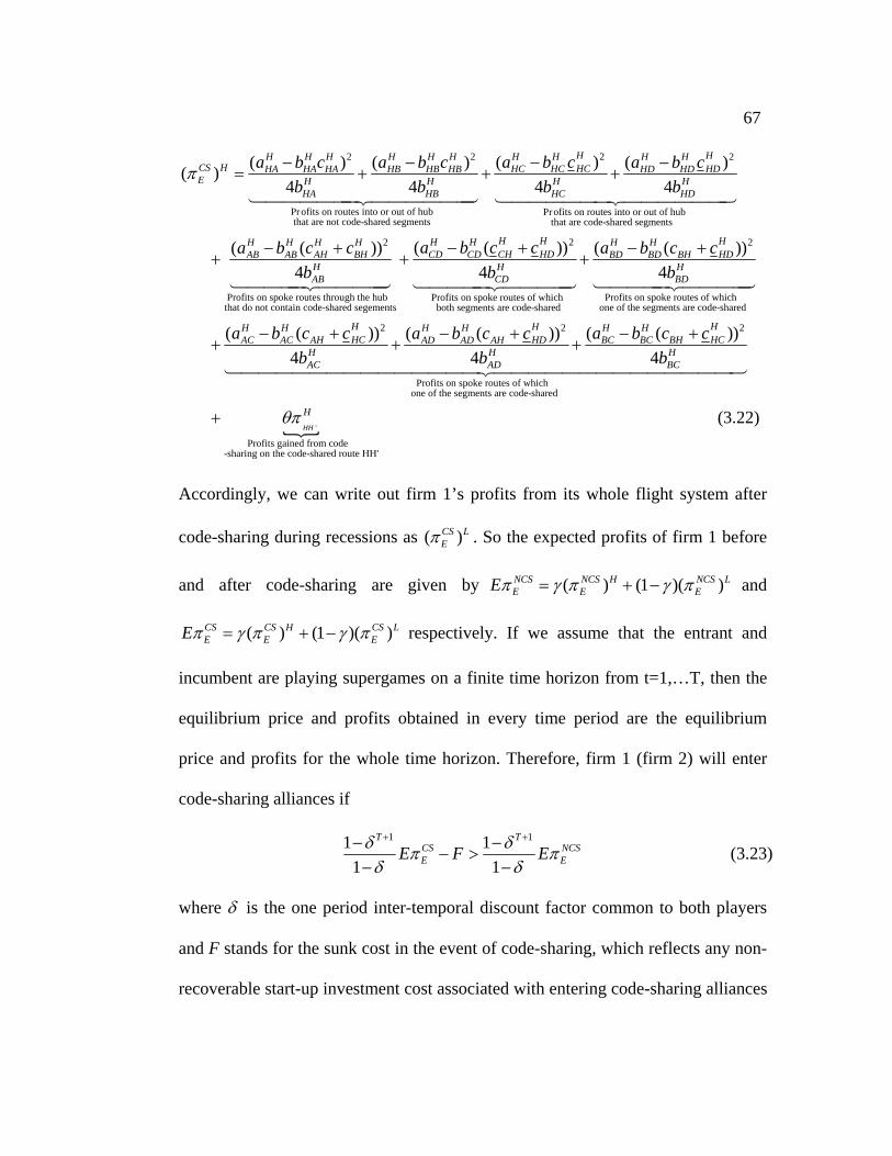
67
22 2
Profits on routes into or out of hub Profits on routes i that are not code-shared segments
( )( ) ( ) (( )4 4 4 4
H HH HH H H H H H H HCS H HCHC HC HDHA HA HA HB HB HB HD HDE H H H H
HA HB HC HD
a b ca b c a b c a b cb b b b
π −− − −= + + +
2)
nto or out of hub that are code-shared segments
2
Profits on spoke routes through the hubthat do not contain code-shared segements
(( ( )) 4
HH H H HCDAB AB AH BH
HAB
a ba b c cb
−− ++ +
2 2
Profits on spoke routes of which Profits on spoke routes of whichone of the segments are code-shared both segments are code-shared
( )) ( (4 4
H H HH H HCH HDCD HDBD BD BHH HCD BD
c c a b c cb b
+ − ++
))
2 22
Profits on spoke routes of which one of the segments are code-shared
( ( )) ( ( )( ( )) 4 4 4
H HHH H H HH HHC HCAC AC AH HD BC BC BHAD AD AH
H H HAC AD BC
a b c c a b c ca b c cb b b
− + − +− ++ + +
)
'
Profits gained from code-sharing on the code-shared route HH'
(3.22)HH
Hθπ+
Accordingly, we can write out firm 1’s profits from its whole flight system after
code-sharing during recessions as ( . So the expected profits of firm 1 before
and after code-sharing are given by and
respectively. If we assume that the entrant and
incumbent are playing supergames on a finite time horizon from t=1,…T, then the
equilibrium price and profits obtained in every time period are the equilibrium
price and profits for the whole time horizon. Therefore, firm 1 (firm 2) will enter
code-sharing alliances if
)CS LEπ
( ) (1 )( )NCS NCS H NCS LE E EEπ γ π γ π= + −
( ) (1 )( )CS CS H CS LE E EEπ γ π γ π= + −
1 11 1
1 1
T TCS NCSEE F Eδ δπ
δ δ
+ +− −− >
− − Eπ (3.23)
where δ is the one period inter-temporal discount factor common to both players
and F stands for the sunk cost in the event of code-sharing, which reflects any non-
recoverable start-up investment cost associated with entering code-sharing alliances
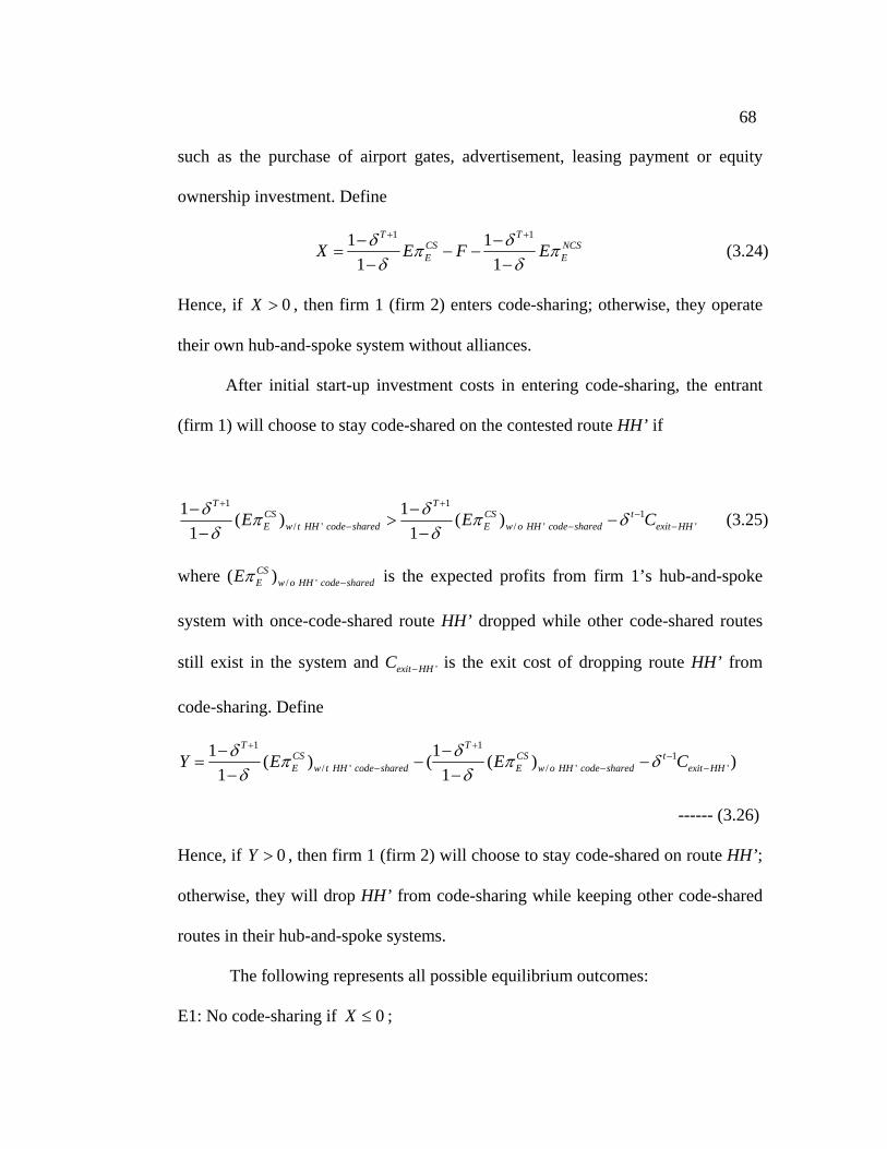
68
such as the purchase of airport gates, advertisement, leasing payment or equity
ownership investment. Define
1 11 1
1 1
T TCS NCSEX E F Eδ δπ
δ δ
+ +− −= − −
− − Eπ (3.24)
Hence, if , then firm 1 (firm 2) enters code-sharing; otherwise, they operate
their own hub-and-spoke system without alliances.
0X >
After initial start-up investment costs in entering code-sharing, the entrant
(firm 1) will choose to stay code-shared on the contested route HH’ if
1 11
/ ' / ' '1 1( ) ( )
1 1
T TCS CS tE w t HH code shared E w o HH code shared exit HHE Eδ δπ π
δ δ
+ +−
− −− −
> −− −
Cδ − (3.25)
where is the expected profits from firm 1’s hub-and-spoke
system with once-code-shared route HH’ dropped while other code-shared routes
still exist in the system and ' is the exit cost of dropping route HH’ from
code-sharing. Define
/ ' ( )CSE w o HH code sharedEπ −
exit HHC −
1 11
/ ' / ' '1 1( ) ( ( )
1 1
T TCS CS tE w t HH code shared E w o HH code shared exit HHY E E Cδ δπ π
δ δ
+ +−
− −− −
= −− −
)δ −−
------ (3.26)
Hence, if , then firm 1 (firm 2) will choose to stay code-shared on route HH’;
otherwise, they will drop HH’ from code-sharing while keeping other code-shared
routes in their hub-and-spoke systems.
0Y >
The following represents all possible equilibrium outcomes:
E1: No code-sharing if 0X ≤ ;
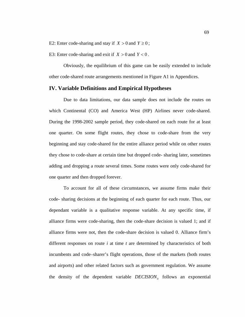
69
E2: Enter code-sharing and stay if and ; 0X > 0Y ≥
E3: Enter code-sharing and exit if and 0X > 0Y < .
Obviously, the equilibrium of this game can be easily extended to include
other code-shared route arrangements mentioned in Figure A1 in Appendices.
IV. Variable Definitions and Empirical Hypotheses Due to data limitations, our data sample does not include the routes on
which Continental (CO) and America West (HP) Airlines never code-shared.
During the 1998-2002 sample period, they code-shared on each route for at least
one quarter. On some flight routes, they chose to code-share from the very
beginning and stay code-shared for the entire alliance period while on other routes
they chose to code-share at certain time but dropped code- sharing later, sometimes
adding and dropping a route several times. Some routes were only code-shared for
one quarter and then dropped forever.
To account for all of these circumstances, we assume firms make their
code- sharing decisions at the beginning of each quarter for each route. Thus, our
dependant variable is a qualitative response variable. At any specific time, if
alliance firms were code-sharing, then the code-share decision is valued 1; and if
alliance firms were not, then the code-share decision is valued 0. Alliance firm’s
different responses on route i at time t are determined by characteristics of both
incumbents and code–sharer’s flight operations, those of the markets (both routes
and airports) and other related factors such as government regulation. We assume
the density of the dependent variable follows an exponential itDECISION
70
distribution with the probability of success denoted as itπ . The classical logistic
regression model is then specified as
0 log( ) ( , ) 1
itit
it
f Xπ β επ
= +−
(3.27)
where X is a matrix of the explanatory variables defined as follows:
Route Characteristics
Because code-shared flights are fundamentally one stop flight service,
market situations in the one stop market on the route level is more comparable for
the analysis than those in the direct or multi-stop or whole flight markets.
Accordingly, we focus on explanatory variables that represent route characteristics
in one stop markets.26
1. Average Yield from Previous Period --- is defined
as the average price per passenger mile in the one stop market on route i in
the previous quarter t-1. Average price is calculated as the weighted average
of per passenger air fare of different air carriers. Staying or dropping
decisions will depend on the average yield of last period. The higher the
average yield from last period; the higher the probability of code-sharing
because of the resulting higher profits from code-sharing (Strassmann, 1990;
Dresner, Lin and Windle, 1996; Dresner, Windle and Yao, 2002);
, 1_ i tONESTOP YIELD −
26 We also used the number of flights, yield and route HHIs calculated from the direct service, multi-stop or the whole market (including direct, one-stop and multi-stop services) on a route as the covariates, but the parameter estimates were strongly insignificant.
71
2. The Number of One Stop Flights from Previous Period ---
, 1i tONESTOPFLTS − is defined as the number of all incumbents’ one stop
flights on route i at time t-1. The larger the number of one stop flights, the
more frequent the service and the higher the service quality, which makes
the alliance firms’ code-shared flights more comparable to the market
incumbents’ one stop flight services, thus leading to the higher probability
of code-sharing (Whinston and Collins, 1992);
3. Route Competition Level from Previous Period --- , 1i tONESTOPRHHI − is
defined as Herfindahl Hirschman Index (HHI) in the one stop market on
route i at time t-1. HHI is calculated by using the number of passengers
carried by individual air carriers on a specific route. According to Sutton
(1991), “Higher concentration implies higher margins and higher
profitability”, so a market with less intense competition pre-entry may be
more profitable and thus be more attractive to entry (Morrison and Winston,
1995; Dresner, Lin and Windle, 1996; Boguslaski, Ito and Lee, 2004; Oh,
2006). However, both Hurdle et al. (1989) and Strassmann (1990) find that
entry is significantly deterred in the highly concentrated airline markets
because of large scale flight operations at hub airports. So the overall effect
of route competition level on the probability of code-sharing is uncertain.27
27 All these three covariates , 1_ i tONESTOP YIELD − , , 1i tONESTOPFLTS − and
are taken the average of their values in the past four quarters from t-1 to t-4 to smooth out the seasonal effect on these variables.
, 1i tONESTOPRHHI −
72
City and Geographical Characteristics
1. Population --- and are the populations at the
endpoints of the Metropolitan Statistical Areas (MSAs) on route i at time t,
which is a proxy for the potential market size. The larger the population,
the higher the travel demand and the higher the probability of code
sharing (Sinclair, 1995; Dresner, Lin and Windle, 1996; Boguslaski, Ito
and Lee, 2004);
itORINPOP itDESTPOP
2. Per Capita Income --- and are per
capita income at both endpoints of MSAs on route i at time t. According
to Morrison (2006), “It’s generally agreed that demand for air travel is
very responsive to changes in income. In particular, the income elasticity
of demand is probably around 1.5.” So we expect the higher per capita
income, the higher the air travel demand and the higher the probability of
code sharing (Dresner, Lin and Windle, 1996; Boguslaski, Ito and Lee,
2004);
itORIINCOME itDESTINCOME
3. Vacation Dummies --- is equal to 1 if one of the endpoint
airports is in Florida, Hawaii, Nevada and Puerto Rico otherwise it is
equal to 0. We expect the coefficient sign to be positively related to the
probability of code- sharing since vacation routes will generate more
passengers than non-vacation routes, all other factors being equal.
(Dresner, Lin and Windle, 1996; Morrison, 2001; Boguslaski, Ito and Lee,
2004)
iVACATION
73
Airport Characteristics
1. Hub Dummies for Code-shared Firms. If either one of the endpoint
airports ( ) or the connecting
airports ( ) are hubs for code-shared firms, then the
value takes 1. This variable represents the advantages of alliance firms’
hub-and-spoke network systems. We expect that the alliance firms’ hubs
at either endpoint or connecting airport will increase the probability of
code-sharing on the routes. Table 3.3 provides a list of hubs for all major
carriers in the US (Borenstein, 1989; Brueckner and Spiller, 1994);
_ _ and _ _iE ORI HUB E DEST HUBi
_ _ iE CONN HUB
2. Slot Control Dummy --- . Four airports in the U.S. have limits on
the number of takeoffs and landings that may take place during any given
hour. They are Chicago O’Hare, New York J.F. Kennedy and La Guardia
and Washington Reagan National Airport. If any of the endpoint or
connecting airports is a slot-controlled airport, then equals 1
otherwise 0. We expect a negative relationship between the probability of
code-sharing and the slot control dummy (Morrison and Winston, 1987;
Strassmann, 1990; Sinclair, 1995; Dresner, Lin and Windle, 1996;
Morrison, 2001; Dresner, Windle and Yao, 2002);
iSLOT
iSLOT
3. Gate Constraints Dummy --- . There are six airports in which
long-term, exclusive use gates are thought to be barriers to entry (GAO
report, 1993). They are Charlotte, Cincinnati, Detroit International,
Minneapolis, Newark and Pittsburgh. If the endpoint or connecting airport
iGATE
74
Table 3.3 U.S. Major Air Carriers and Their Hubs and Focus Cities
Major Carriers Hubs Second Hubs Focus Cities
American Airlines DFW, ORD, MIA, STL, SJU JFK, LGA BOS, LAX, RDU Alaska Airlines SEA, ANC, PDX, LAX SFO Continental Airlines IAH, EWR, CLE Delta Air Lines ATL, SLC, CVG, JFK LAX MCO, LGA, BOSNorthwest Airlines DTW, MSP, MEM IND, HNL United Airlines ORD, DEN, IAD, SFO, LAX US Airways CLT, PHL, PHX, LAS DCA, LGA, PIT
Southwest Airlines
LAS, MDW, PHX, BWI, OAK,HOU, DAL,LAX, MCO, SAN
America West PHX, LAS, PHL, CLT PIT DCA, LGA, BOS ATA Airlines MDW HNL,OAK
JetBlue Airways JFK, BOS, FLL, OAK, IAD
Horizon Air SEA, PDX, LAX DEN Frontier Airlines DEN
is a gate-constrained airport, then equals 1 otherwise 0. We iGATE
assume code-sharing will be deterred in the airports with gate constraints
due to airport congestion (Dresner, Windle and Yao, 2002).
Time Characteristics
1. Quarterly Dummies --- are used to
control for seasonal fixed effects (Dresner, Li and Windle, 1996; Morrison,
2001);
, and t tWINTER SPRING SUMMERt
2. Time since the Initial Alliance --- is used to measure how long (in
years) the initial code-sharing alliance has been in place. For instance, if the
tTIME
75
code-share alliance began in 1994, then =5 in year 1998, 6 in year
1999, 7 in year 2000, 8 in year 2001 and 9 in year 2002. On one hand, we
expect a negative relationship between alliance duration and the probability of
code-sharing because the longer the time, the more information firms will
have about the profitability of alliances. As time passes, market situations
may change dramatically, firms’ financial situations and operating strategies
may change, government policy may change, etc. On the other hand, the
longer firms stay in an alliance, the better the reputation of the alliance and
the lower the continuation cost so there could be a positive relationship
between the time and the probability of code-sharing. Thus, the expected sign
of the time coefficient is uncertain.
tTIME
Lagged Dependent Variables
1. Code-Sharing Decisions from Last Period --- Firms’
decisions to stay or drop code-sharing at time t may depend on their decisions
from last period. We expect that the decision of whether or not to code-share
on route i at time t-1 may positively affect the decision on route i at the
current time t;
, 1i tDECISION −
IV. Data Source
The whole data sample has 39260 quarterly observations on a total of 1963
routes code-shared by Continental and America West Airlines at some time during
1998Q1 to 2002Q4 period. Every observation is route and time specific. Table 3.4
shows the descriptive statistics.
76
Table 3.4 Descriptive Statistics
Variables (Descriptions and Units) Mean
Std
DECISIONit (Equals 1 if the alliance firms code-shared on route i, otherwise 0) 0.186246 0.38931ONESTOPYIELDit-1 (Average air fare from t-1 in dollars per passenger mile in the one-stop market of route i) 0.064730.026428ONESTOPFLTSit-1 (All incumbents' one-stop flights from t-1 on route i) 401.1002331.6551ONESTOPRHHIit-1 (HHI from t-1 in the one-stop market of route i ) 2827.13 1611.28INCOME_ORIGINit (Per capita income in dollars at the MSA of the origin airport on route i) 18050.73 3211.91INCOME_DESTit (Per capita income in dollars at the MSA of the destination airport on route i) 17979.46 3277.1POP_ORIGINit (Population at the MSA of the origin airport on route i) 3907724 4456131POP_DESTit (Population at the MSA of the destination airport on route i) 3933258 4561028SLOTi (Equals 1 if either the endpoint or the connecting airport is a slot-controlled airport on route i) 0.0524710.222977GATEi (Equals 1 if either the endpoint or the connecting airport is a gate-constrained airport on route i) 0.2710140.444489VACATIONi (Equals 1 if either the endpoint or connecting airport on route i is in FL, HI or NV, otherwise 0) 0.4034640.490599E_ORI_HUBi (Equals 1 if the origin airport on route i is the alliance firms' dominated hub or focus city) 0.3336730.471531E_CONN_HUBi (Equals 1 if the connecting airport on route i is the alliance firms' dominated hub or focus city) 0.8772290.328179E_DEST_HUBi (Equals 1 if the destination airport on route i is the alliance firms’ dominated hub or focus city) 0.3173710.465459WINTERt (Equals 1 if the quarter is in Jan-Mar, otherwise 0) 0.250.433018SPRINGt (Equals 1 if the quarter is in Apr-Jun, otherwise 0) 0.250.433018SUMMERt (Equals 1 if the quarter is in Jul-Sep, otherwise 0) 0.250.433018TIMEt (Equals 5 if in year 1998, 6 in 1999, 7 in 2000, 8 in 2001, 9 in 2002) 71.414232
All the dollar values are deflated by Consumer Price Index (1982-84=100).
The data for the number of passengers and per passenger air fares for
individual carriers on route i at time t are from Bureau of Transportation Statistics
77
(BTS) US Department of Transportation (DOT) Origin and Destination Survey
DB1B Market, a 10% ticket random sample data set. is
calculated as the average price per passenger mile on route i in its one stop market
at time t where average price is calculated as the weighted average of the per
passenger air fare for all air carriers operating on that route. The data for the code-
sharing decision are identified from the same data set by tracking each
route once code-shared by Continental and America West Airlines quarter by
quarter. The data for the number of one stop flights and the
calculation of route concentration are from DB1B Market. Hub
dummies are identified from each air carrier’s website.
itONESTOPYIELD
itDECISION
itONESTOPFLTS
itONESTOPRHHI
28 The data for
population and and per capita income _ itPOP ORIGIN _ itPOP DEST
_ itINCOME ORIGIN and _ itINCOME DEST at origin and destination airport
MSAs are from Bureau of Economic Analysis US Department of Commerce. The
slot control and gate constraints dummies are obtained from reports by US General
Accounting Office (1993).
V. Econometric Models and Empirical Results
Following Molenberghs and Verbeke (2005) for the study of discrete
longitudinal data, we apply three different models including Marginal Models,
Subject-specific Models and Transition Models for the analysis of the discrete
28 We also use the number of flights, yield and route HHI calculated from the direct service market or the whole market, which includes direct, one-stop and multi-stop services on a route as the covariates, but the parameter estimates are strongly insignificant.
78
longitudinal data set, in which the dependent variable is non-Gaussian repeated
binary measures. 29 Each model has its own model assumptions and estimation
methods, therefore resulting in different numerical values and interpretations of
coefficient estimates.
V.1. Subject-specific Models
In subject-specific models, when responses are binary, the effect of
covariates on the response probabilities is conditional upon the level of the subject-
specific effect. A unit change in the covariate translates into an appropriate change
in probability, keeping the level of the subject-specific effect fixed (Neuhaus,
Kalbfleisch and Hauck, 1991). Even though subject-specific parameters can be
dealt with either as fixed effects or as random effects, the fixed effects approach is
in many cases flawed.30 So we use the Generalized Linear Mixed Models (GLIMM)
proposed by Breslow and Clayton (1993) in this paper, which is the most
frequently used random effects model in the context of discrete repeated
measurements.
29 In longitudinal settings, each individual has a vector of responses with a natural (time) ordering among the components. Non-Gaussian longitudinal cases include repeated binary or ordinal data, or longitudinally measured counts. 30 Neyman and Scott (1948) show that in a fixed-effect model, if the number of subjects is getting larger while the number of time points remains constant, the number of parameters is increasing at the same rate as the sample size, which leads to inconsistency of the so-obtained maximum likelihood estimates. This is a well-known result in the context of logistic regression for binary data. Breslow and Day (1989) have an extensive discussion in this context.
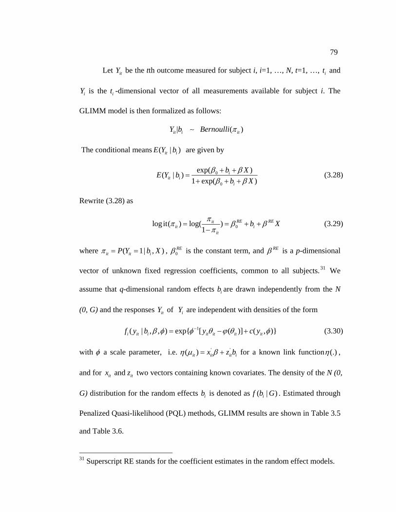
79
Let be the tth outcome measured for subject i, i=1, …, N, t=1, …, and
is the -dimensional vector of all measurements available for subject i. The
GLIMM model is then formalized as follows:
itY it
iY it
| ( )it i itY b Bernoulli π∼
The conditional means are given by ( | )it iE Y b
0
0
exp( )( | )1 exp( )
iit i
i
b XE Y bb X
β ββ β+ +
=+ + +
(3.28)
Rewrite (3.28) as
0log it( ) log( )1
RE REitit i
it
b Xππ βπ
= = + +−
β (3.29)
where ( 1| , )it it iP Y b Xπ = = , 0REβ is the constant term, and REβ is a p-dimensional
vector of unknown fixed regression coefficients, common to all subjects.31 We
assume that q-dimensional random effects are drawn independently from the N
(0, G) and the responses of are independent with densities of the form
ib
itY iY
1( | , , ) exp{ [ ( )] ( , )}i it i it it it itf y b y c yβ φ φ θ ϕ θ−= − + φ (3.30)
with φ a scale parameter, i.e. ' '( )it it it ix z bη μ β= + for a known link function (.)η ,
and for and it itx z two vectors containing known covariates. The density of the N (0,
G) distribution for the random effects is denoted asib ( | )if b G . Estimated through
Penalized Quasi-likelihood (PQL) methods, GLIMM results are shown in Table 3.5
and Table 3.6.
31 Superscript RE stands for the coefficient estimates in the random effect models.
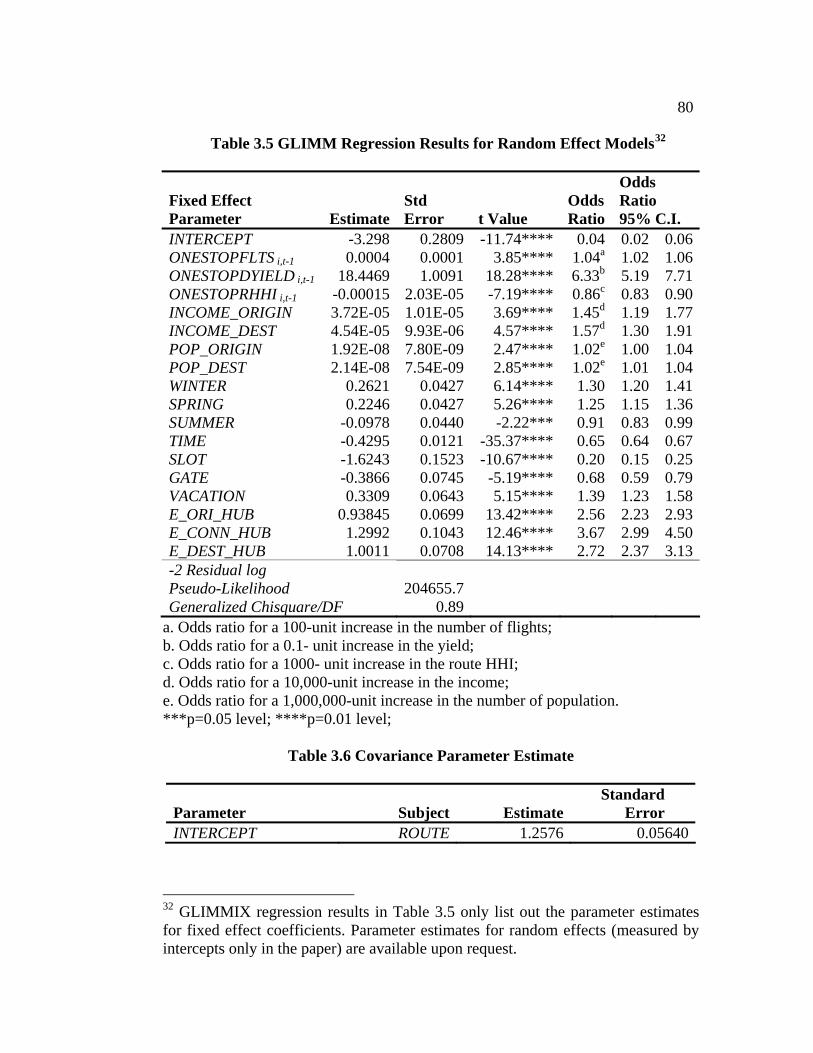
80
Table 3.5 GLIMM Regression Results for Random Effect Models32
Fixed Effect Parameter Estimate
Std Error t Value
Odds Ratio
Odds Ratio 95% C.I.
INTERCEPT -3.298 0.2809 -11.74**** 0.04 0.02 0.06ONESTOPFLTS i,t-1 0.0004 0.0001 3.85**** 1.04a 1.02 1.06ONESTOPDYIELD i,t-1 18.4469 1.0091 18.28**** 6.33b 5.19 7.71ONESTOPRHHI i,t-1 -0.00015 2.03E-05 -7.19**** 0.86c 0.83 0.90INCOME_ORIGIN 3.72E-05 1.01E-05 3.69**** 1.45d 1.19 1.77INCOME_DEST 4.54E-05 9.93E-06 4.57**** 1.57d 1.30 1.91POP_ORIGIN 1.92E-08 7.80E-09 2.47**** 1.02e 1.00 1.04POP_DEST 2.14E-08 7.54E-09 2.85**** 1.02e 1.01 1.04WINTER 0.2621 0.0427 6.14**** 1.30 1.20 1.41SPRING 0.2246 0.0427 5.26**** 1.25 1.15 1.36SUMMER -0.0978 0.0440 -2.22*** 0.91 0.83 0.99TIME -0.4295 0.0121 -35.37**** 0.65 0.64 0.67SLOT -1.6243 0.1523 -10.67**** 0.20 0.15 0.25GATE -0.3866 0.0745 -5.19**** 0.68 0.59 0.79VACATION 0.3309 0.0643 5.15**** 1.39 1.23 1.58E_ORI_HUB 0.93845 0.0699 13.42**** 2.56 2.23 2.93E_CONN_HUB 1.2992 0.1043 12.46**** 3.67 2.99 4.50E_DEST_HUB 1.0011 0.0708 14.13**** 2.72 2.37 3.13-2 Residual log Pseudo-Likelihood 204655.7 Generalized Chisquare/DF 0.89
a. Odds ratio for a 100-unit increase in the number of flights; b. Odds ratio for a 0.1- unit increase in the yield; c. Odds ratio for a 1000- unit increase in the route HHI; d. Odds ratio for a 10,000-unit increase in the income; e. Odds ratio for a 1,000,000-unit increase in the number of population. ***p=0.05 level; ****p=0.01 level;
Table 3.6 Covariance Parameter Estimate
Parameter Subject EstimateStandard
Error INTERCEPT ROUTE 1.2576 0.05640
32 GLIMMIX regression results in Table 3.5 only list out the parameter estimates for fixed effect coefficients. Parameter estimates for random effects (measured by intercepts only in the paper) are available upon request.
81
GLIMM regression results show that on a specific route, the number of
flights and the average yields on the one stop market in the previous quarter are
significant factors affecting the probability of code-sharing. The probability of
code-sharing is higher when the yield is higher and the number of flights is
increasing on the one stop market from the previous period. For a given route, the
odds of code-sharing increases 6.33 times for every increase of 0.1 dollar in the
yield (5.19 times to 7.71 times at 95% confidence interval) and 1.04 times (1.02
times to 1.06 times at 95% confidence interval.) for every increase of 100 flights on
the one stop market. In contrast to Sutton (1991), Morrison and Winston (1995),
Dresner, Lin and Windle (1996), Boguslaski, Ito and Lee (2004) and Oh (2006),
who found that higher concentration induces entry, we find that route concentration
level has a negative impact on the probability of code-sharing: the higher the
concentration in the one stop market, the lower the probability of code-sharing,
consistent with Hurdle et al (1989) and Strassmann (1990). Large scale operations
from the market incumbents on a specific highly concentrated route in their one
stop market could deter the probability of code-sharing greatly. The odds of code-
sharing increase only 0.86 times (0.83 times to 0.90 times at a 95% confidence
interval) for every increase of 1000 in route competition as measured by the HHI.
Regression results also tell that as expected, on a specific route, the
probability of code-sharing is lower if the origin and connecting airports on the
route are slot-controlled or have gate constraints. This means that airport
congestion measured by slot control and gate constraints are significant entry
82
barriers for code-sharing on individual routes, consistent with previous findings by
Morrison and Winston (1987), Strassmann (1990), Sinclair (1995) and etc.
Specifically, the occurrence of code-sharing is only 0.20 as likely to occur on a
route with slot-controlled airports as on a route without slot control, given other
factors constant. This difference could be as little as 0.15 or as much as 0.25 with a
95% confidence interval. Compared with routes whose origin and connecting
airports have no gate constraints, the odds of code-sharing are only 0.68 times the
odds on the route whose airports are with gate constraints. The change in the odds
could be as little as 0.59 or as much as 0.79 with a 95% confidence interval.
Whether individual route is a vacation route also turns out to be an important
factor affecting the probability of code-sharing. The probability of code-sharing is
found here to be higher on a vacation route than on a non-vacation route. For a
given route, the odds of code-sharing, ( 1itDECISION = ) if it is a vacation route,
are 1.39 times the odds of code-sharing if it is not a vacation one, holding other
things constant (1.23 times to 1.58 times at 95% confidence interval). Consistent
with previous studies (Dresner, Lin and Windle, 1996; Morrison, 2001; Boguslaski,
Ito and Lee, 2004), this result supports the hypothesis that vacation routes generate
more passengers than non-vacation routes, therefore increasing the probability of
code-sharing. Carriers may choose to code-share on vacation routes because of the
route density.
On a specific route, whether or not its endpoint or connecting airports is an
alliance firm hub strongly affects the probability of code-sharing. The probability
83
of code- sharing is higher if the airports are alliance firm hubs than if not. In
particular, the odds of code-sharing when the origin, connecting and destination
airports are alliance firm hubs or focus cities on an individual route are 2.56, 3.67
and 2.72 times the odds of code- sharing when these airports are not their hubs or
focus cities respectively. This is consistent with studies by Bailey and William
(1989), Borenstein (1989, 1990 and 1991) and Brueckner and Spiller (1994) who
argue that airport dominance is an important source of market power and monopoly
rent in the airline industry. Alliance firms make use of their hubs to combine their
existing operating systems and compete with the market incumbents.
Results also show that on a given route, per capita income and population at
the endpoint MSAs are significant factors affecting the code-sharing decision. The
higher the per capita income and population on a specific route, the higher
probability of code- sharing because of the resulting higher travel demand. On a
given route, the odds of code sharing increase 1.45 and 1.57 times respectively as
the per capita income at the origin and destination MSAs increases by 10,000
dollars. The odds of code-sharing increase 1.02 and 1.02 times for every increase of
1,000,000 persons in the number of origin and destination MSA population.
As time passes, the probability of code-sharing tends to decrease as expected.
The odds of code-sharing increase 0.65 times on a specific route (0.64 times to 0.67
times at 95% confidence interval.) as one more year passes by. Seasonal effects
significantly affect the code-share decisions with the lower probability of code-
sharing in the summer and higher probability in the winter and spring. On a specific
84
route, the odds of code-sharing in the winter and spring are 1.30 times and 1.25
times the odds of code-sharing in other seasons, respectively. The odds of code-
sharing in the summer are only 0.91 times the odds of code-sharing in other seasons
for a given route. This may be because code- sharing helps generate traffic in off
season whereas demand is seasonally high in summer.
V.2. Marginal Models (or Population-Averaged Models)
In contrast to the subject-specific models, in marginal models, a unit
change in the covariates translates into a change in the response probability,
marginal over the subject-specific effects. It is assumed that
( )it itY Bernoulli π∼
The marginal average evolution is obtained from averaging (3.28) over the
random effects, i. e.
( )itE Y
33
0
0
exp( )( ) [ ( | )] [ ]1 exp( )
iit it i
i
b XE Y E E Y b Eb X
β ββ β+ +
= =+ + +
(3.30)
Rewrite (3.30) as
0log it( ) log( )1
M Mitit
it
Xππ βπ
= = +−
β (3.31)
where ( 1| )it itP Y Xπ = = , 0Mβ is the constant term, and Mβ is the vector of
unknown regression coefficients. 34 Compared with the random effect models,
33 “In case the random intercept variability is large, parameters from fitting marginal and random effect models will be very different, while equal parameter values hold if the variance of the random effect equals zero” (Molenberghs and Verbeke, 2005).
85
where the vector REβ models the evolution of each individual subject respectively,
Mβ tells on average, in marginal models, the success probability evolved in the
population.
Generalized Estimating Equations (GEE) initially proposed by Liang and
Zeger (1986) are the best and most frequently used marginal or population-
averaged model for correlated discrete repeated data. “Correlated” means that the
components of are assumed correlated but individual subjects and itY iY iY
( )j i jY ≠ are independent, i.e., code- share decisions on route i and route j are
independent but code-sharing decisions on route i at time t and t-1 (or t-k) may be
correlated. GEE method combines estimating equations for the regression
parameters associated with the expected values of an individual’s vector of binary
responses with moment-based estimation for the association between pairs of
outcomes in terms of marginal correlations. The score equations for a multivariate
marginal normal model ( , )i iY N X Viβ∼ are given by35
' 1/ 2 1/ 2 1
1( ) ( ) ( ) 0
N
i i i i i ii
S X A R A Y Xβ β−
=
= − =∑ (3.32)
The covariance matrix of is modeled as iY
(3.33) 1/ 2 1/ 2( ) ( )i i i i iV Y A R Aφ α=
34 Superscript M stands for the coefficient estimates in the marginal models. 35 iX includes a constant term.
86
where is an diagonal matrix with iA in n× i ( )itv μ as the tth diagonal element and
iR is an marginal correlation matrix of that is unknown and needs to be
estimated. When there is truly no correlation between the repeated measurements
for the subject i, then GEE is reduced to the Generalized Linear Models (GLM)
(McCullagh and Nelder, 1989).
in n× i
iY
36
As for the assumption of the correlation structure, the nature of the equally
spaced time periods in our data set for individual subjects means that a time
dependence correlation structure such as AR(1) or M-dependent (Stationary)
process is among the best alternatives. Pan (2001) derives a new measure called the
Quasilikelihood under the Independence Model Information Criterion (QIC) to
choose the best correlation structure from alternatives.37 The smallest QIC statistic
provides the most efficient correlation structure.38 Our calculations shows that the
independence structure has the smallest QIC, even smaller than the QIC
36 For a detailed description and application of GEE methodology, please refer to Hardin and Hilbe (2003) and Molenberghs and Verbeke (2005). 37 Please refer to Appendix 2 for the specifications of different working correlation structures including Fixed, Independent, Autoregressive-AR(1), M-dependent, Exchangeable and Unstructured structures and corresponding estimators. 38 Even though QIC provides a good measurement to choose the most efficient correlation structure, it “should not be blindly followed”. “When there is some motivating scientific evidence of a particular correlation structure, then that specification should be used” (Hardin and Hilbe, 2003). QIC statistics in Table 3.7 show that the difference among Independence, M-dependent(1) and AR(1) is very tiny.
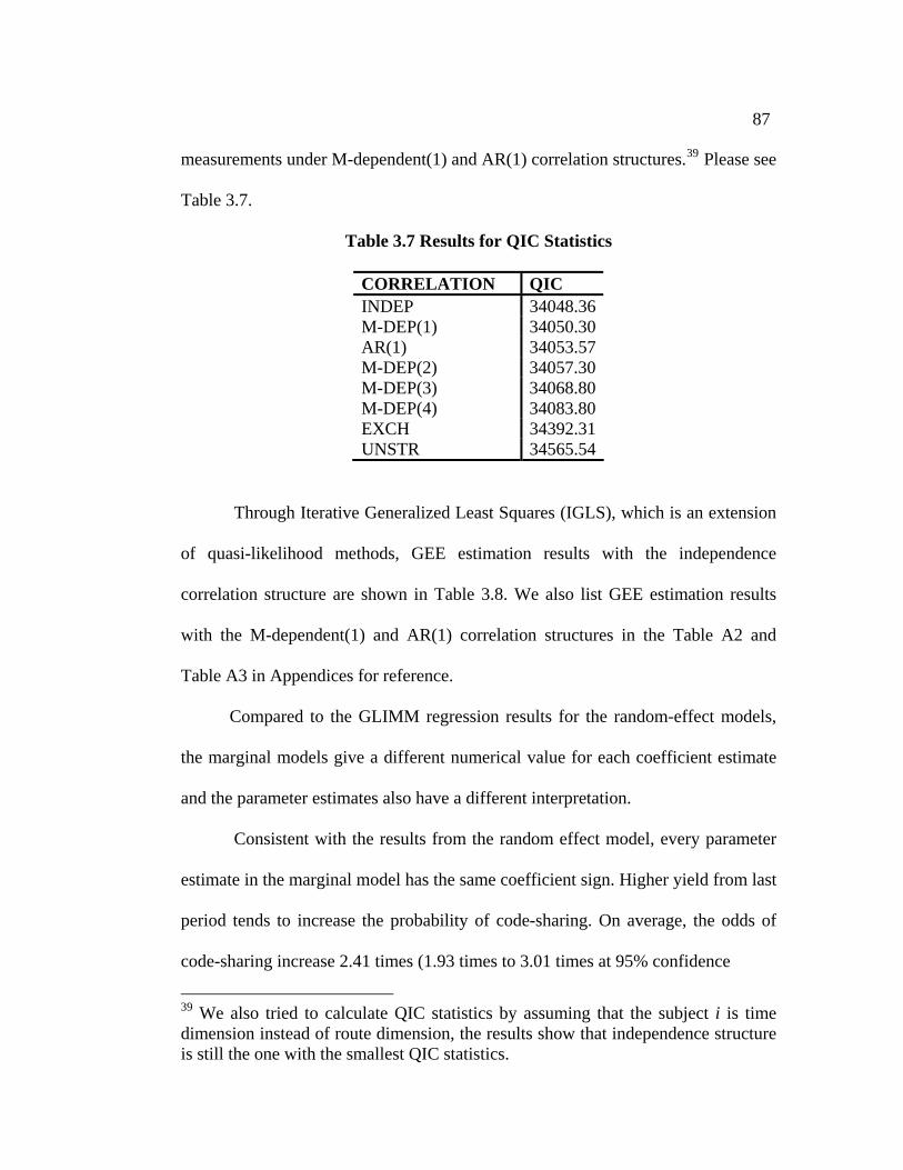
87
measurements under M-dependent(1) and AR(1) correlation structures.39 Please see
Table 3.7.
Table 3.7 Results for QIC Statistics
CORRELATION QIC INDEP 34048.36M-DEP(1) 34050.30AR(1) 34053.57M-DEP(2) 34057.30M-DEP(3) 34068.80M-DEP(4) 34083.80EXCH 34392.31UNSTR 34565.54
Through Iterative Generalized Least Squares (IGLS), which is an extension
of quasi-likelihood methods, GEE estimation results with the independence
correlation structure are shown in Table 3.8. We also list GEE estimation results
with the M-dependent(1) and AR(1) correlation structures in the Table A2 and
Table A3 in Appendices for reference.
Compared to the GLIMM regression results for the random-effect models,
the marginal models give a different numerical value for each coefficient estimate
and the parameter estimates also have a different interpretation.
Consistent with the results from the random effect model, every parameter
estimate in the marginal model has the same coefficient sign. Higher yield from last
period tends to increase the probability of code-sharing. On average, the odds of
code-sharing increase 2.41 times (1.93 times to 3.01 times at 95% confidence
39 We also tried to calculate QIC statistics by assuming that the subject i is time dimension instead of route dimension, the results show that independence structure is still the one with the smallest QIC statistics.
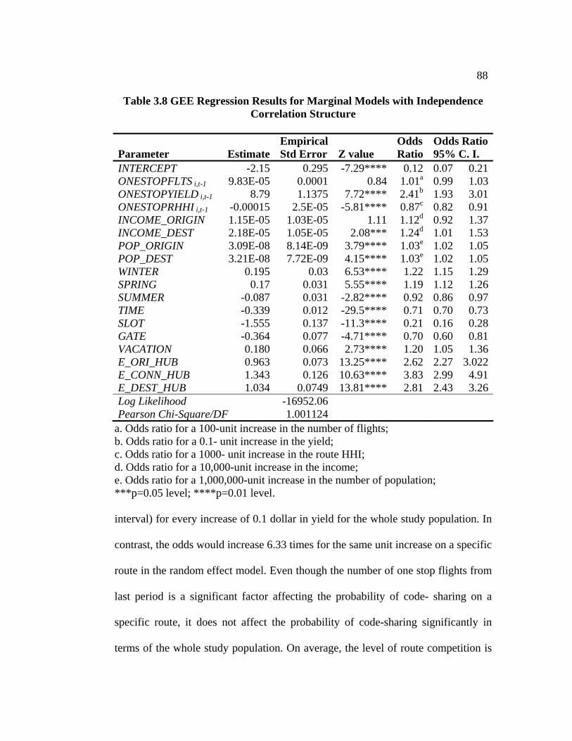
88
Table 3.8 GEE Regression Results for Marginal Models with Independence Correlation Structure
Parameter EstimateEmpirical Std Error Z value
Odds Ratio
Odds Ratio 95% C. I.
INTERCEPT -2.15 0.295 -7.29**** 0.12 0.07 0.21ONESTOPFLTS i,t-1 9.83E-05 0.0001 0.84 1.01a 0.99 1.03ONESTOPYIELD i,t-1 8.79 1.1375 7.72**** 2.41b 1.93 3.01ONESTOPRHHI i,t-1 -0.00015 2.5E-05 -5.81**** 0.87c 0.82 0.91INCOME_ORIGIN 1.15E-05 1.03E-05 1.11 1.12d 0.92 1.37INCOME_DEST 2.18E-05 1.05E-05 2.08*** 1.24d 1.01 1.53POP_ORIGIN 3.09E-08 8.14E-09 3.79**** 1.03e 1.02 1.05POP_DEST 3.21E-08 7.72E-09 4.15**** 1.03e 1.02 1.05WINTER 0.195 0.03 6.53**** 1.22 1.15 1.29SPRING 0.17 0.031 5.55**** 1.19 1.12 1.26SUMMER -0.087 0.031 -2.82**** 0.92 0.86 0.97TIME -0.339 0.012 -29.5**** 0.71 0.70 0.73SLOT -1.555 0.137 -11.3**** 0.21 0.16 0.28GATE -0.364 0.077 -4.71**** 0.70 0.60 0.81VACATION 0.180 0.066 2.73**** 1.20 1.05 1.36E_ORI_HUB 0.963 0.073 13.25**** 2.62 2.27 3.022E_CONN_HUB 1.343 0.126 10.63**** 3.83 2.99 4.91E_DEST_HUB 1.034 0.0749 13.81**** 2.81 2.43 3.26Log Likelihood -16952.06 Pearson Chi-Square/DF 1.001124
a. Odds ratio for a 100-unit increase in the number of flights; b. Odds ratio for a 0.1- unit increase in the yield; c. Odds ratio for a 1000- unit increase in the route HHI; d. Odds ratio for a 10,000-unit increase in the income; e. Odds ratio for a 1,000,000-unit increase in the number of population; ***p=0.05 level; ****p=0.01 level. interval) for every increase of 0.1 dollar in yield for the whole study population. In
contrast, the odds would increase 6.33 times for the same unit increase on a specific
route in the random effect model. Even though the number of one stop flights from
last period is a significant factor affecting the probability of code- sharing on a
specific route, it does not affect the probability of code-sharing significantly in
terms of the whole study population. On average, the level of route competition is
89
still an important variable affecting the firms’ code sharing decisions. A high route
HHI from the previous period decreases the probability of code-sharing. The odds
of code-sharing increase 0.87 times (0.82 to 0.91 times at 95% confidence interval)
for the whole route sample when the HHI increases by 1000, a result very similar to
the odds change (0.86 times) on a specific route.
Vacation routes tend to increase the probability of code-sharing for the
whole sample. The odds of code-sharing on the vacation routes are 1.20 times (1.05
times to 1.36 times at 95% confidence interval) the odds of code sharing on the
non-vacation routes, a little smaller than the odds change (1.39 times) on a specific
route. For the covariates --- slot-control and gate constraints, the marginal model
also shows that they decrease the probability of code-sharing. On average, the odds
of code-sharing from slot-controlled and gate-constrained routes are only 0.21 and
0.69 times the odds on routes without airport congestion, similar to the odds
changes (0.20 and 0.68 times respectively) on a specific route.
Alliance firm hub dominance plays an important role in their code-sharing
decisions. For the whole route sample, the odds of code-sharing when the origin,
connecting and destination airports are alliance firms’ hubs or focus cities are
respectively 2.62, 3.83 and 2.81 times the odds of code-sharing in the case that
alliance firms do not enjoy hub advantages in these airports, a result a little bigger
than the odds changes (2.56, 3.67 and 2.72 times) on a specific route.
For the whole study sample, population at both endpoint MSAs also has a
significant effect on the probability of code-sharing but only per capita income at
90
the destination airport MSAs significantly affects the probability of code sharing.
Results from the marginal model show that the effect of the parameter estimates for
population on the log-odds are much bigger with 3.09E-08 and 3.21E-08 than those
obtained for a specific route with 1.93E-08 and 2.15E-08 in the random effect
model while the effect of those of the per capita income is much smaller with
1.15E-05 and 2.18E-05 than those for a specific route with 3.73E-05 and 4.54E-05
even though the difference in the odds changes is tiny between two models due to
the very small numerical values of these coefficient estimates. Seasons also have a
significant effect on the probability of code- sharing in the marginal model. The
numerical values of the odds change for the whole study population is similar to
those for a specific route. Time has the same negative effect on the probability of
code-sharing for the whole study population as on a specific route and with a
similar odds change as well.
V.3. Transition Models
In a transition model, a measurement in a longitudinal sequence is
described as a function of previous outcomes (or a subset of previous outcomes),
i.e., conditional on the history
itY
1 ,( ,..., )it i i th Y Y 1−= . We assume
( )it itY Bernoulli π∼
Decomposing the outcome Tit it itY Tμ ε= + (“T” standing for transition), the mean and
variance of a transition model can be written in terms of the history : ith
(3.34) ( | )Tit it itE Y hμ =
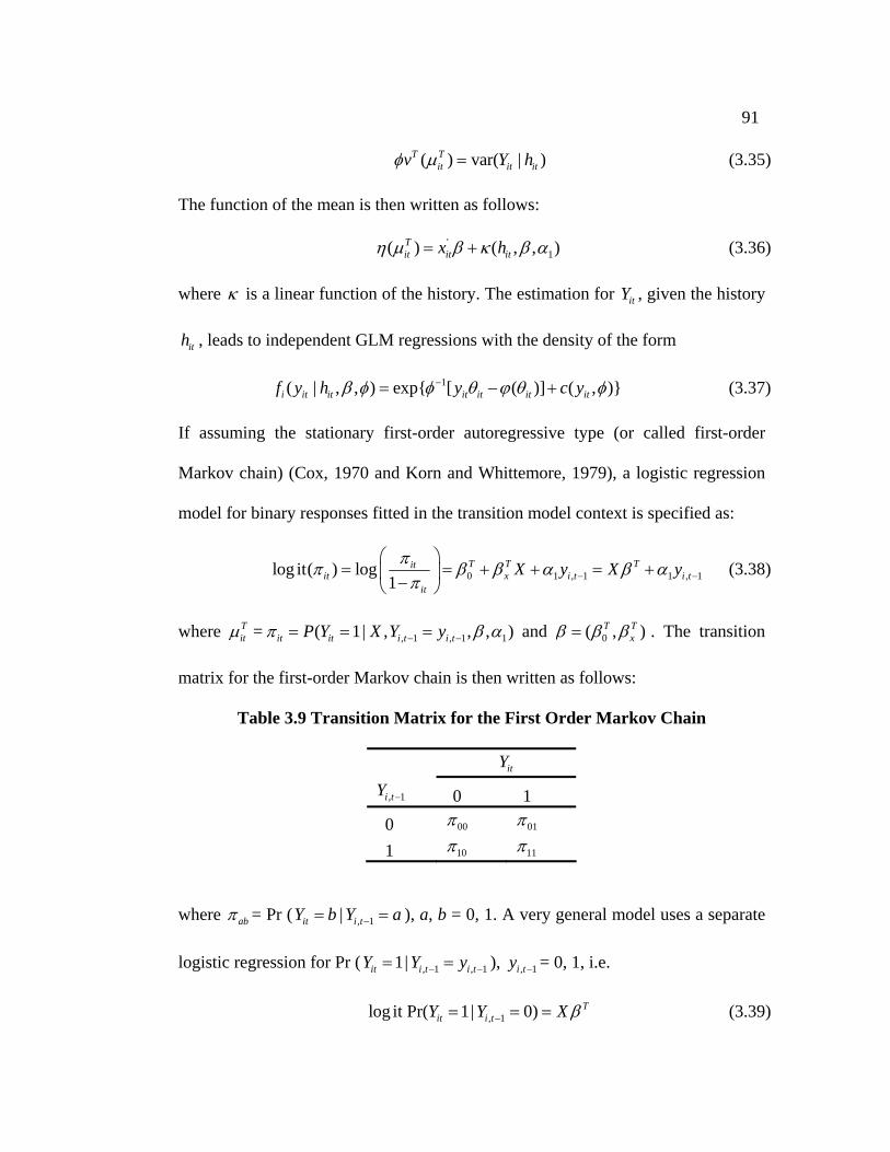
91
(3.35) ( ) var( | )T Tit it itv Yφ μ = h
)
The function of the mean is then written as follows:
'1( ) ( , ,T
it it itx hη μ β κ β= + α (3.36)
where is a linear function of the history. The estimation for , given the history
, leads to independent GLM regressions with the density of the form
κ itY
ith
1( | , , ) exp{ [ ( )] ( , )}i it it it it it itf y h y c yβ φ φ θ ϕ θ−= − + φ (3.37)
If assuming the stationary first-order autoregressive type (or called first-order
Markov chain) (Cox, 1970 and Korn and Whittemore, 1979), a logistic regression
model for binary responses fitted in the transition model context is specified as:
0 1 , 1log it( ) log1
T T Titit x i t i t
it1 , 1X y X yππ β β α β
πα− −
⎛ ⎞= = + + = +⎜ ⎟−⎝ ⎠
(3.38)
where Titμ = , 1 , 1 1( 1| , , ,it it i t i tP Y X Y y )π β α− −= = = and 0( ,T T )xβ β β= . The transition
matrix for the first-order Markov chain is then written as follows:
Table 3.9 Transition Matrix for the First Order Markov Chain
itY
, 1i tY − 0 1 0 00π 01π
1 10π 11π
where abπ = Pr ( ), a, b = 0, 1. A very general model uses a separate
logistic regression for Pr (
, 1|it i tY b Y a−= =
, 1 , 11|it i t i tY Y y− −= = ), , 1i ty − = 0, 1, i.e.
, 1log it Pr( 1| 0) Tit i tY Y X β−= = = (3.39)
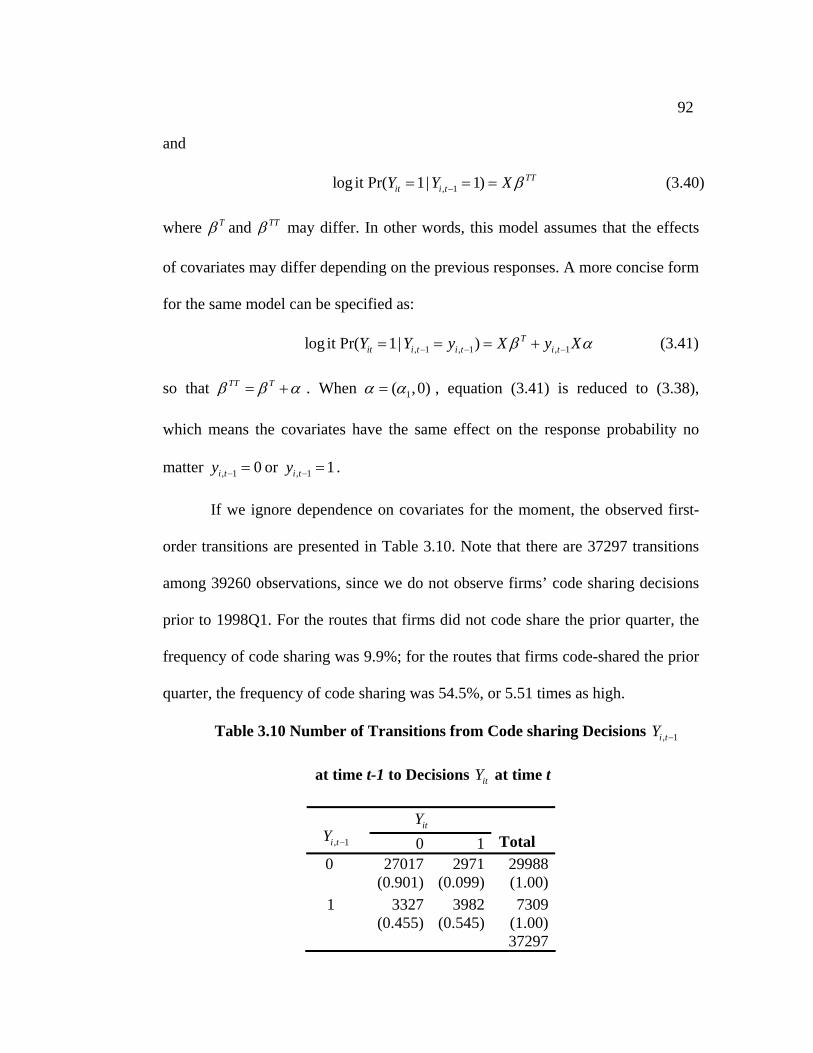
92
and
, 1log it Pr( 1| 1) TTit i tY Y X β−= = = (3.40)
where Tβ and TTβ may differ. In other words, this model assumes that the effects
of covariates may differ depending on the previous responses. A more concise form
for the same model can be specified as:
, 1 , 1 , 1log it Pr( 1| ) Tit i t i t i tY Y y X y Xβ α− − −= = = + (3.41)
so that TT Tβ β= +α . When 1( ,0)α α= , equation (3.41) is reduced to (3.38),
which means the covariates have the same effect on the response probability no
matter or . , 1 0i ty − = , 1 1i ty − =
If we ignore dependence on covariates for the moment, the observed first-
order transitions are presented in Table 3.10. Note that there are 37297 transitions
among 39260 observations, since we do not observe firms’ code sharing decisions
prior to 1998Q1. For the routes that firms did not code share the prior quarter, the
frequency of code sharing was 9.9%; for the routes that firms code-shared the prior
quarter, the frequency of code sharing was 54.5%, or 5.51 times as high.
Table 3.10 Number of Transitions from Code sharing Decisions , 1i tY −
at time t-1 to Decisions at time t itY
itY Y , 1i t− 0 1
Total
0 27017 2971 29988 (0.901) (0.099) (1.00) 1 3327 3982 7309 (0.455) (0.545) (1.00) 37297
93
Estimated by pseudo-likelihood (PL) methods, transition model results are
presented in Table 3.11 and 3.12. Empirical results show that as expected, the
number of flights, yield and the route HHI on one stop markets are still important
factors affecting a firm’s decision but only the effect of the route HHI on the
probability of code-sharing significantly depends on the firms’ code-sharing
decisions in the prior quarter. A larger number of flights on one-stop markets
increase the probability of code-sharing with the odds increasing 1.02 times (1.00
to 1.03 times at a 95% confidence interval) for every increase of 100 more flights.
Higher yield increases the probability of code-sharing with the odds increasing 1.71
times (1.47 to 1.98 times at a 95% confidence interval) for every increase of $0.1 in
the yield. A higher level of route competition from the previous quarter decreases
the probability of code-sharing at time t more than if firms were in code-sharing at
t-1. Specifically, for every increase of 1000 in the HHI, the odds increase 0.90
times (0.84 to 0.95 times at a 95% confidence interval) if the firms code- shared in
the prior quarter but increase 0.94 times (0.91 to 0.97 times at a 95% confidence
interval.) if firms did not.
Slot-controlled airports decrease the probability of code-sharing with a
stronger effect if firms code-shared during the prior quarter. The odds of code-
sharing on slot- controlled routes are 0.54 times (0.44 to 0.65 times at a 95%
confidence interval) the odds on the routes without slot-controlled airports if firms
did not code-share at t-1 while this change in odds is 0.14 times (0.11 to 0.20 times
at a 95% confidence interval) if firms stay code-shared during the previous
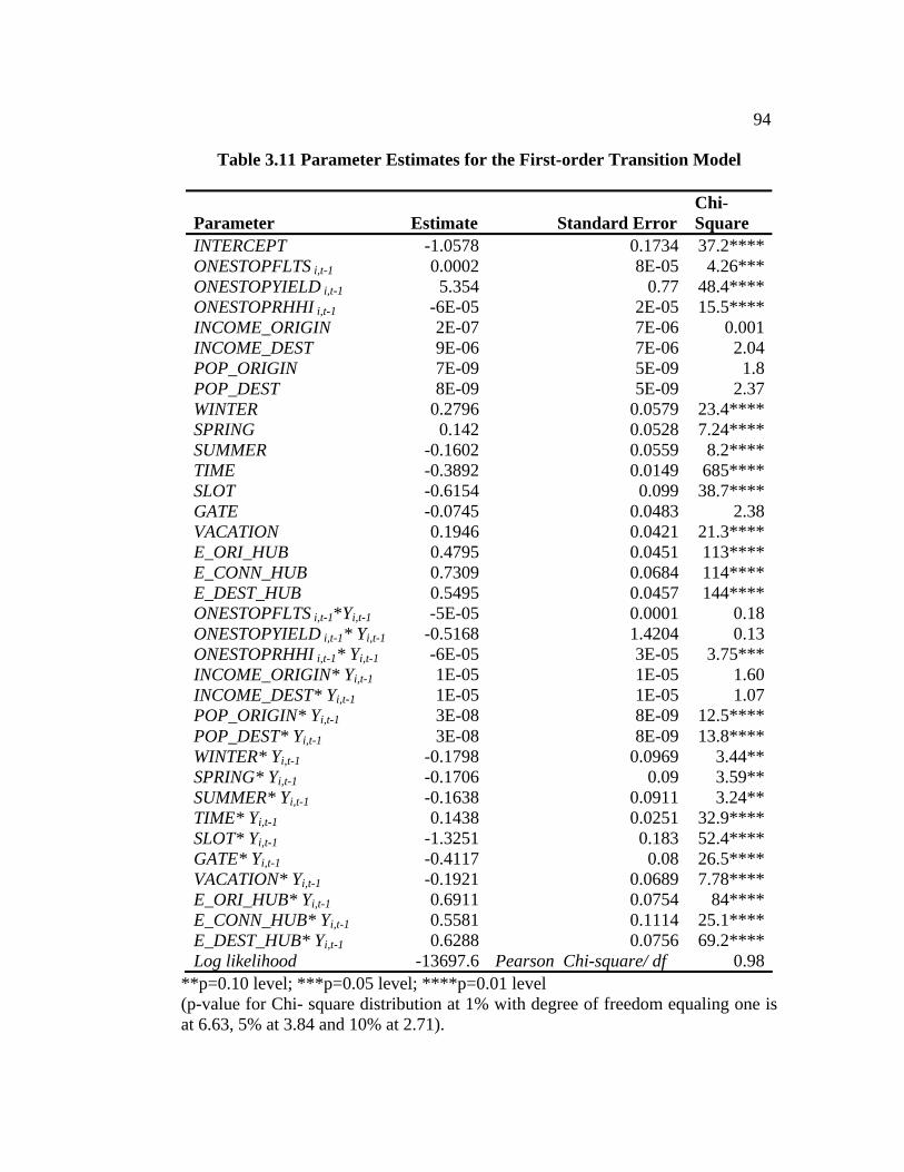
94
Table 3.11 Parameter Estimates for the First-order Transition Model
Parameter Estimate Standard Error Chi-Square
INTERCEPT -1.0578 0.1734 37.2****ONESTOPFLTS i,t-1 0.0002 8E-05 4.26***ONESTOPYIELD i,t-1 5.354 0.77 48.4****ONESTOPRHHI i,t-1 -6E-05 2E-05 15.5****INCOME_ORIGIN 2E-07 7E-06 0.001INCOME_DEST 9E-06 7E-06 2.04POP_ORIGIN 7E-09 5E-09 1.8POP_DEST 8E-09 5E-09 2.37WINTER 0.2796 0.0579 23.4****SPRING 0.142 0.0528 7.24****SUMMER -0.1602 0.0559 8.2****TIME -0.3892 0.0149 685****SLOT -0.6154 0.099 38.7****GATE -0.0745 0.0483 2.38VACATION 0.1946 0.0421 21.3****E_ORI_HUB 0.4795 0.0451 113****E_CONN_HUB 0.7309 0.0684 114****E_DEST_HUB 0.5495 0.0457 144****ONESTOPFLTS i,t-1*Yi,t-1 -5E-05 0.0001 0.18ONESTOPYIELD i,t-1* Yi,t-1 -0.5168 1.4204 0.13ONESTOPRHHI i,t-1* Yi,t-1 -6E-05 3E-05 3.75***INCOME_ORIGIN* Yi,t-1 1E-05 1E-05 1.60INCOME_DEST* Yi,t-1 1E-05 1E-05 1.07POP_ORIGIN* Yi,t-1 3E-08 8E-09 12.5****POP_DEST* Yi,t-1 3E-08 8E-09 13.8****WINTER* Yi,t-1 -0.1798 0.0969 3.44**SPRING* Yi,t-1 -0.1706 0.09 3.59**SUMMER* Yi,t-1 -0.1638 0.0911 3.24**TIME* Yi,t-1 0.1438 0.0251 32.9****SLOT* Yi,t-1 -1.3251 0.183 52.4****GATE* Yi,t-1 -0.4117 0.08 26.5****VACATION* Yi,t-1 -0.1921 0.0689 7.78****E_ORI_HUB* Yi,t-1 0.6911 0.0754 84****E_CONN_HUB* Yi,t-1 0.5581 0.1114 25.1****E_DEST_HUB* Yi,t-1 0.6288 0.0756 69.2****Log likelihood -13697.6 Pearson Chi-square/ df 0.98
**p=0.10 level; ***p=0.05 level; ****p=0.01 level (p-value for Chi- square distribution at 1% with degree of freedom equaling one is at 6.63, 5% at 3.84 and 10% at 2.71).
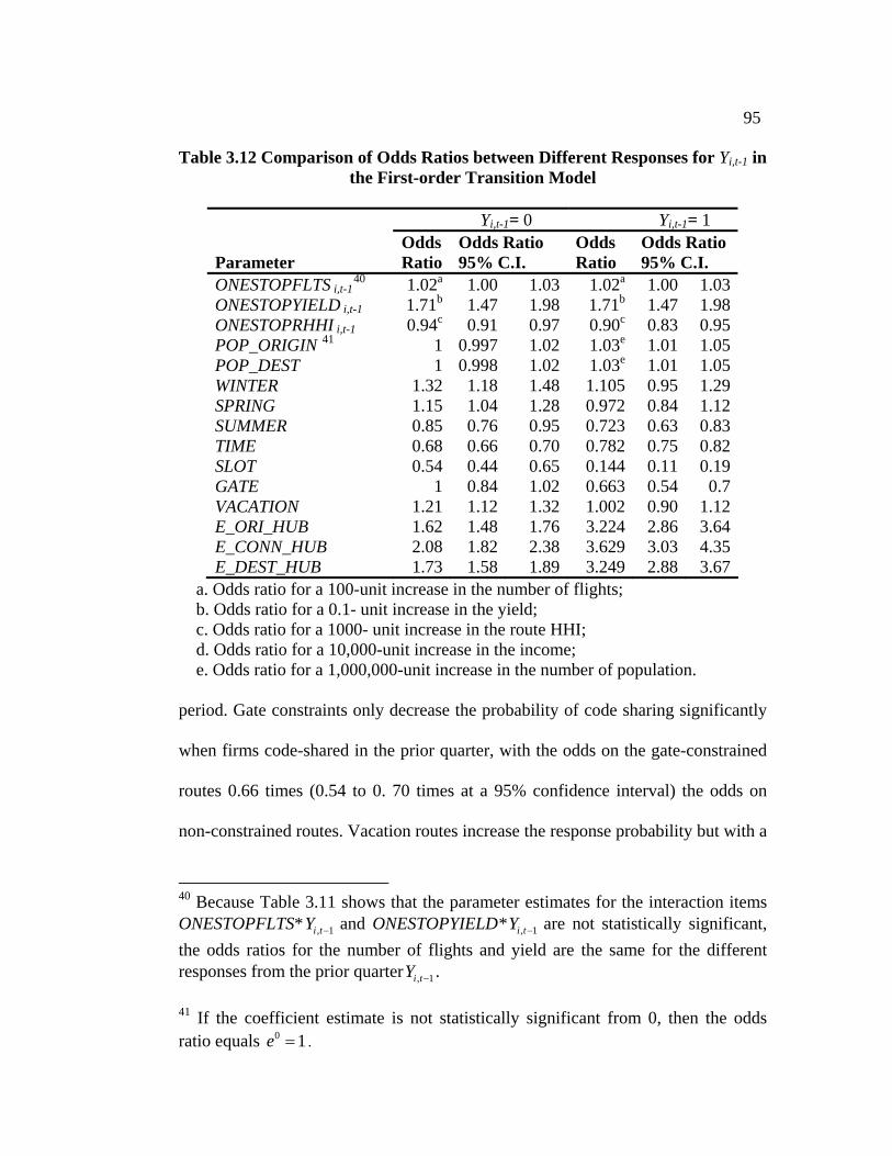
95
Table 3.12 Comparison of Odds Ratios between Different Responses for Yi,t-1 in the First-order Transition Model
Yi,t-1= 0 Yi,t-1= 1
Parameter Odds Ratio
Odds Ratio 95% C.I.
Odds Ratio
Odds Ratio 95% C.I.
ONESTOPFLTS i,t-140 1.02a 1.00 1.03 1.02a 1.00 1.03
ONESTOPYIELD i,t-1 1.71b 1.47 1.98 1.71b 1.47 1.98ONESTOPRHHI i,t-1 0.94c 0.91 0.97 0.90c 0.83 0.95POP_ORIGIN 41 1 0.997 1.02 1.03e 1.01 1.05POP_DEST 1 0.998 1.02 1.03e 1.01 1.05WINTER 1.32 1.18 1.48 1.105 0.95 1.29SPRING 1.15 1.04 1.28 0.972 0.84 1.12SUMMER 0.85 0.76 0.95 0.723 0.63 0.83TIME 0.68 0.66 0.70 0.782 0.75 0.82SLOT 0.54 0.44 0.65 0.144 0.11 0.19GATE 1 0.84 1.02 0.663 0.54 0.7VACATION 1.21 1.12 1.32 1.002 0.90 1.12E_ORI_HUB 1.62 1.48 1.76 3.224 2.86 3.64E_CONN_HUB 2.08 1.82 2.38 3.629 3.03 4.35E_DEST_HUB 1.73 1.58 1.89 3.249 2.88 3.67
a. Odds ratio for a 100-unit increase in the number of flights; b. Odds ratio for a 0.1- unit increase in the yield; c. Odds ratio for a 1000- unit increase in the route HHI; d. Odds ratio for a 10,000-unit increase in the income; e. Odds ratio for a 1,000,000-unit increase in the number of population. period. Gate constraints only decrease the probability of code sharing significantly
when firms code-shared in the prior quarter, with the odds on the gate-constrained
routes 0.66 times (0.54 to 0. 70 times at a 95% confidence interval) the odds on
non-constrained routes. Vacation routes increase the response probability but with a
40 Because Table 3.11 shows that the parameter estimates for the interaction items ONESTOPFLTS* and ONESTOPYIELD*, 1i tY − , 1i tY − are not statistically significant, the odds ratios for the number of flights and yield are the same for the different responses from the prior quarter , 1i tY − . 41 If the coefficient estimate is not statistically significant from 0, then the odds ratio equals . 0 1e =
96
smaller effect if firms code-shared in the previous period. The odds of code-sharing
on the vacation routes are 1.00 times (0.90 to 1.12 times at 95% C.I.) the odds on
the non-vacation routes if firms stay code-shared at time t-1 and this change
increases to 1.22 times if firms did not.
Seasons still play a significant role in affecting the response probability. If
firms did not code-share in the prior quarter, the odds of code-sharing in the winter
and spring are 1.32 and 1.15 times the odds of code-sharing in other seasons and
the odds of code- sharing in the summer are only 0.85 times the odds of code-
sharing in other seasons. These changes in odds are 1.11, 0.97, 0.72 times
respectively if firms code-shared at t-1, which means that the seasonal effects of the
winter and spring on the probability of code-sharing becomes smaller and the effect
of the summer becomes larger if firms code-shared in the prior quarter. The
probability of code-sharing decreases with time. But the odds of code-sharing
increases 0.78 times if firms code-shared in the prior quarter and increases 0.68
times if firms do not.
Alliance firms take full advantage of their hubs in the code-shared route
arrangement. The effect of airport dominance on the probability of code-sharing is
stronger if firms code-shared in the prior quarter than if not. In particular, if firms
did not code-share at t-1, the odds of code-sharing when the origin, connecting and
destination airports are alliance firms’ hubs or focus cities are 1.62, 2.08, 1.73
times the odds of code-sharing when alliance firms do not enjoy hub dominance in
97
these airports. These changes in odds increase to 3.22, 3.63, 3.25 times respectively
if firms code-shared in the prior quarter.
Population affects the probability of code-sharing significantly only when
firms code-shared in the prior quarter. The odds of code-sharing increase 1.03 and
1.30 times for every increase of 1,000,000 in population at the endpoint MSAs. Per
capita incomes do not affect the response probability significantly no matter firms
code-shared in the previous period or not.
VI. Conclusions
Our empirical results show that a successful code-sharing depends on many
factors. The larger the number of flights and the higher the yield on one-stop
markets, the higher the probability of code-sharing. Airport dominance is an
important factor that affects alliance firm code-sharing decisions. Alliance firms
tend to code-share flight routes whose origin, connecting or destination airports are
their hub cities. In addition, we find that both airport congestion measured by slot-
control and gate constraints and a high route concentration level on one-stop
markets are important barriers that limit firm’s use of code-sharing. Firms prefer to
code-share on vacation routes because of the larger number of potential passengers.
Population and per capita incomes are also important determinants of successful
code-sharing. The probability of code sharing tends to be higher in the markets
with more population and higher income. The airline industry is characterized by
seasonal demand, which significantly affects code-sharing decisions.
98
Reference:
Abramowitz, A.D. and Brown, S.M. (1993), “Market Share and Price Determination in the Contemporary Airline Industry”, Review of Industrial Organization, V8(4), 419-433; Armantier, O. and Richard, O. (2005a), “Evidence on Pricing from the Continental Airlines and Northwest Airlines Code-Share Agreement", D. Lee (eds.) Advances in Airline Economics V1, 2006. Elsevier Publisher; ------(2005b), “Domestic Airline Alliances and Consumer Welfare”, Working papers, University of Montreal, Canada; Baily, E.E. and Baumol, W.J. (1984), “Deregulation and the Theory of Contestable Markets”, Yale Journal on Regulation V1(2), 111-137; Baily, E.E. and Panzar, J.G. (1981), “The Contestability of Airline Markets during the Transition to Deregulation”, Law and Contemporary Problem, V44(1), 125-145; Baily, E.E. and Williams, J.R. (1988), “Sources of Rent in the Deregulated Airline Industry”, Journal of Law and Economics V XXXI, 173-202; Bamberger, G.E. and Carlton, D.W. (2006), “Predation and the Entry and Exit of Low-fare Carriers”, Lee, D. (eds), Advances in Airlines Economics, V1, 2006, Elsevier Publisher; Bamberger, G.E., Carlton, D.W. and Neumann, L.R. (April 2004), “An Empirical Investigation of the Competitive Effects of Domestic Airline Alliances”, Journal of Law and Economics, V XLVII, 195-222; Bain, J.S. (1956), Barriers to New Competition, Cambridge, MA, Harvard University Press; Baumol, W.J. (1982), “Contestability: An Uprising in the Theory of Industrial Structure”, American Economic Review, V72, 1-15; Bennet, R. and Craun, J. (1993), “The Airline Deregulation Evolution Continues: The Southwest Effect”, Office of Aviation Analysis, U.S. Department of Transportation, Washington, D.C.; Berry, S.T. (1990), “Airport Presence as Product Differentiation”, American Economic Review Papers and Proceedings, V80(2), 394-399;
99
------(1992), “Estimation of a Model of Entry in the Airline Industry”, Econometrica, V60(4), 889-917; Boguslaski, C., Ito, H. and Lee, D. (2004), “Entry Patterns in the Southwest Airlines Route System”, Review of Industrial Organization, V25, 317-350; Borenstein, S. (1989), “Hubs and High Fares: Dominance and Market Power in the US Airline Industry”, Rand Journal of Economics, V20, 344-365; ------(1990), “Airline Mergers, Airport Dominance and Market Power”, American Economic Review Papers and Proceedings, V80(2), 400-404; ------(1991), “The Dominant Firm Advantage in Multi-product Industries: Evidence from the US Airlines”, Quarterly Journal of Economics, V106(4), 1237-1266; Breslow, N.E. and Clayton, D.G. (1993), “Approximate Inference in Generalized Linear Mixed Models”, Journal of the American Statistical Association, V88, 9-25; Breslow, N.E. and Day, N. E. (1989), Statistical Methods in Cancer Research Volume 1: The Analysis of Case-control Studies, International Agency for Research on Cancer, Scientific Publications 32; Brueckner, J.K. (2001), “The Economics of International Code-sharing: an Analysis of Airline Alliances,” International Journal of Industrial Organization, V19, 1475-1498; ------(2003), “International Airfares in the Age of Alliances: The Effects to Code-sharing and Antitrust Immunity”, Review of Economic Statistics, V85, 105-118; Brueckner, J.K., Dyer, N.J. and Spiller, P.T. (1992), “Fare Determination in Airline Hub-and-Spoke Networks”, Rand Journal of Economics, V23, 309-333; Brueckner, J.K. and Spiller, P.T. (Oct 1994), “Economies of Traffic Density in the Deregulated Airline Industry”, Journal of Law and Economics, V37(2), 379-415; Brueckner, J.K. and Whalen, W.T. (October 2000), “The Price Effect of International Airline Alliances”, Journal of Law and Economics, V XLIII, 503-544; Caves, D.W., Christensen, L.R. and Tretheway, M.W. (1984), “Economies of Density versus Economies of Scale: Why Trunk and Local Service Airline Costs Differ”, Rand Journal of Economics, V15(4), 471-489;
100
Chua, C.L., Kew, H and Yong, J (2005), “Airline Code-sharing Alliances and Costs: Imposing Concavity on Translog Cost Function Estimation”, Review of Industrial Organization V26, 461-487; Cox, D.R. (1970), Analysis of Binary Data, Chapman and Hall, London; Dresner, M., Windle, R. and Yao, Y. (2002), “Airport Barriers to Entry in the US”, Journal of Transport Economics and Policy, V36(2), 389-405; Dresner, M., Lin J.C. and Windle, R. (1996), “The Impact of Low-cost Carriers on Airport and Route Competition”, Journal of Transport Economics and Policy, V30, 309-328; Du, Y., McMullen, B. S. and Kerkvliet, J. (2008), “Assessing the Economic Impact of Domestic Airline Codesharing: A Case Study of the ATA and Southwest Airlines Agreement”, working paper, Oregon State University; Evans, W.N. and Kessides, I.N. (1993), “Localized Market Power in the US Airline Industry”, Review of Economics and Statistics, V75, 66-75; Gayle, P.G. (2006), “Airline Code-share Alliances and Their Competitive Effects”, Journal of Law and Economics, forthcoming; Hardin, J. W. and Hilbe, J.M. (2003), Generalized Estimating Equations, Boca Raton, Florida, Chapman & Hall/CRC; Hassin, O. and Shy, O. (2004), “Code-sharing Agreements and Interconnections in Markets for International Flights”, Review of International Economics, V12(3), 337-352; Hendricks, K., Piccione, M. and Tan, G. (1997), “Entry and Exit in Hub-spoke Networks”, Rand Journal of Economics, V28(2), 291-303; Hurdle, G.J., Johnson, R.L., Joskow, A.S., Werden, G.J. and Williams, M.A. (1989), “Concentration, Potential Entry, and Performance in the Airline Industry”, Journal of Industrial Economics, V38(2), 119-139; Korn, E.L. and Whittemore, A.S. (1979), “Methods for analyzing panel studies of acute health effects of air pollution”, Biometrics, V35, 795-802; Liang, K. Y. and Zeger, S. L. (1986), “Longitudinal Data Analysis Using Generalized Linear Models”, Biometrika, V73, 13-22;
101
McCullagh, P. and Nelder, J.A. (1989), Generalized Linear Models, London, Chapman & Hall; Molenberghs, G. and Verbeke, G. (2005), Models for Discrete Longitudinal Data, New York, Springer Science & Business Media, Inc; Morrison, S.A. (2001), “Actual, Adjacent, and Potential Competition---Estimating the Full Effect of Southwest Airlines”, Journal of Transport Economics and Policy, V35(2), 239-256; Morrison, S.A. and Winston, C.(1990), “The Dynamics of Airline Pricing and Competition”, American Economic Review Papers and Proceedings, V80(2), 389-393; ------(1995), The Evolution of the Airline Industry, Washington, D.C., The Brookings Institution; ------ (1987), “Empirical Implications and Tests of the Contestability Hypothesis”, Journal of Law and Economics, V XXX, 53-66; Neuhaus, J. M., Kalbfleisch, J. D., and Hauck, W.W. (1991), “A comparison of cluster-specific and population-averaged approaches for analyzing correlated binary data”, International Statistical Review, V59, 25-35; Neyman, J. and Scott, E. L. (1948), “Consistent Estimates Based on Partially Consistent Observations”, Econometrica, V16, 1-32; Oh, J. (2006), “‘Flight under Radar’: Southwest Airlines and Incumbents’ Response to Entry”, Journal of Economic Development, V31(1), 149-171; Oum, T.H., Park, J.H. and Zhang, Y.(1996), “The Effects of Airline Code-sharing Agreements on Firm Conduct and International Air Fares”, Journal of Transport Economics and Policy, V30(2), 187-202; Oum, T.H., Zhang, A., and Zhang, Y. (1995), “Airline Network Rivalry”, Canadian Journal of Economics, V28, 836-857; Pan, W. (2001), “Akaike’s Information Criterion in Generalized Estimating Equations”, Biometrics, V57, 120-125; Park, J.H. (1997), “The Effects of Airline Alliances on Markets and Economic Welfare”, Transportation Research Part E: Logistics and Transportation Review, V33(3), 181-195;
102
Park, J.H., Park, N.K. and Zhang, A. (2003), “The Impact of International Alliances on Rival Firm Value: A Study of the British Airways US Air Alliance”, Transportation Research Part E: Logistics and Transportation Review, V39(1), 1-18; Park, J.H. and Zhang, A. (2000), “An Empirical Analysis of Global Airline Alliances: Cases in North Atlantic Markets”, Review of Industrial Organization, V16: 367-383; Park, J.H., Zhang, A. and Zhang, Y.(2001), “Analytical Models of International Alliances in the Airline Industry”, Transportation Research Part B: Methodological, V35(9), 865-886; Richards, K. (1996), “The Effect of Southwest Airlines on U.S. Airlines Markets”, in B.S. McMullen (ed.) Research in Transportation Economics, V4, 33-47; Shy, O. (1996), Industrial Organization: Theory and Applications, MIT Press; Siegfried, J. and Evans, L.B. (1994), “Empirical Studies of Entry and Exit: A Survey of the Evidence”, Review of Industrial Organization, V9(2), 121-155; Sinclair, R.A. (1993), An Empirical Model of Entry and Exit in Airline Markets, PhD Dissertation, University of Pittsburgh; ------(1995), “An Empirical Model of Entry and Exit in Airline Markets”, Review of Industrial Organization, V10(5), 541-557; Strassmann, D.L. (1990), “Potential Competition in the Deregulated Airlines”, Review of Economics and Statistics, V72(4), 696-702; Sutton, J. (1991), Sunk Costs and Market Structure: Price Competition, Advertising and the Evolution of Concentration, Cambridge, MA: MIT Press; Windle, R. and Dresner, M. (1995), “The Short and Long Run Effects of Entry on US Domestic Air Routes”, Transportation Journal, V35, 14-25; Winston, M. and Collins, S.C. (1992), “Entry and Competitive Structure in Deregulated Airline Markets: An Event Study Analysis of People Express”, Rand Journal of Economics, V23(4), 445-462; U.S. General Accounting Office (1993), “Airline Competition: Higher Fares and Less Competition Continue at Concentrated Airports”;

103
Chapter 4
Conclusion
104
This research provides evidence that the overall effect of complementary
code-share agreements can be beneficial. Air fare decreased and passenger volumes
increased on non-stop markets served by the incumbent carriers on Denver routes
following entry onto those routes by ATA and Southwest Airlines through a
complementary code-share agreement. Further, both consumer and producer
surpluses were found to increase on these routes after initiation of the code-share
agreement. These results are similar to those of previous research that document the
competitive impact of direct entry onto routes by Southwest Airlines --- it appears
that entry via code-hearing may be a less costly way to promote competitive results
in markets similar to Denver. Thus, policy makers interested in promoting airline
market competition and industry efficiency should be careful not to dismiss code-
sharing as a way to promote competition in markets where direct entry may not be
a feasible option.
As far as routes that are likely to result in successful code-share
arrangements contracting carriers try to take advantage of their hub dominance to
build code-shared routes with their partners. Since there is previous research
(Bailey and William (1988), Borenstein (1989, 1990, 1991), Berry (1990, 1992),
Evans and Kessides (1993) and Oum, Zhang and Zhang (1995)) that suggests there
may be monopoly rents enjoyed by carriers serving concentrated hubs, policy
makers including the Department of Transportation and the Department of Justice
should pay special attention to the code-shared routes proposed to or from alliance
firms’ hubs to insure again the possible exercise of market power on individual
105
routes. High route level concentration was found to discourage carriers from
staying in a code-share arrangement after initial entry, which could be a sign for
policy makers to be alert for anti-competitive behavior on the part of market
incumbents on highly concentrated routes. High average yields on a route were
found to induce alliance firms to stay in a code-share arrangement.
Government policies to deal with airport congestion by instituting slot
controls and gate restrictions have generally discouraged firms from entering into
and staying in code-share agreements on those routes. Thus, regulators need to
continue to monitor competitive conditions at those airports where gate and slot
controls are in effect as this not only discourages direct entry but also code-share
entry which is another way that competitive outcomes can be achieved.
106
Bibliography
Abramowitz, A.D. and Brown, S.M. (1993), “Market Share and Price Determination in the Contemporary Airline Industry”, Review of Industrial Organization, V8(4), 419-433; Armantier, O. and Richard, O. (2005a), “Evidence on Pricing from the Continental Airlines and Northwest Airlines Code-Share Agreement", Advances in Airline Economics V1, 2006. Elsevier Publisher, edited by Darin Lee; ------(2005b), “Domestic Airline Alliances and Consumer Welfare”, Working papers, University of Montreal, Canada; Baily, E.E. and Baumol, W.J. (1984), “Deregulation and the Theory of Contestable Markets”, Yale Journal on Regulation V1(2), 111-137; Baily, E.E. and Panzar, J.G. (1981), “The Contestability of Airline Markets during the Transition to Deregulation”, Law and Contemporary Problem, V44(1), 125-145; Baily, E.E. and Williams, J.R. (1988), “Sources of Rent in the Deregulated Airline Industry”, Journal of Law and Economics V XXXI, 173-202; Bamberger, G.E. and Carlton, D.W. (2006), “Predation and the Entry and Exit of Low-fare Carriers”, Lee, D. (eds), Advances in Airlines Economics, V1, 2006, Elsevier Publisher; Bamberger, G.E., Carlton, D.W. and L.R. Neumann (April 2004), “An Empirical Investigation of the Competitive Effects of Domestic Airline Alliances”, Journal of Law and Economics, V XLVII, 195-222; Bain, J.S. (1956), Barriers to New Competition, Cambridge, MA, Harvard University Press; Baumol, W.J. (1982), “Contestability: An Uprising in the Theory of Industrial Structure”, American Economic Review, V72, 1-15; Bennet, R. and Craun, J. (1993), “The Airline Deregulation Evolution Continues: The Southwest Effect”, Office of Aviation Analysis, U.S. Department of Transportation, Washington, D.C.; Berry, S.T. (1990), “Airport Presence as Product Differentiation”, American Economic Review Papers and Proceedings, V80(2), 394-399;
107
------(1992), “Estimation of a Model of Entry in the Airline Industry”, Econometrica, V60(4), 889-917; Boguslaski, C., Ito, H. and Lee, D. (2004), “Entry Patterns in the Southwest Airlines Route System”, Review of Industrial Organization, V24, 317-350; Borenstein, S. (1989), “Hubs and High Fares: Dominance and Market Power in the US Airline Industry”, Rand Journal of Economics, V20(3), 344-365; ------(1990), “Airline Mergers, Airport Dominance and Market Power”, American Economic Review Papers and Proceedings, V80(2), 400-404; ------(1991), “The Dominant Firm Advantage in Multi-product Industries: Evidence from the US Airlines”, Quarterly Journal of Economics, V106 (4), 1237-1266; Borenstein, S and Netz, J. (1999), “Why do all the flights leave at 8 am: Competition and Departure-time Differentiation in the Airline Markets”, International Journal of Industrial Organization, V17(5), 611-640; Brander, J.A. and Zhang, A. (Winter 1990), “Market Conduct in the Airline Industry: An Empirical Investigation,” Rand Journal of Economics, V21(4), 217-233; -------- (1993), “Dynamic Oligopoly Behavior in the Airline Industry,” International Journal of Industrial Organization, V11, 407-435; Breslow, N.E. and Clayton, D.G. (1993), “Approximate Inference in Generalized Linear Mixed Models”, Journal of the American Statistical Association, V88, 9-25; Breslow, N.E. and Day, N. E. (1989), Statistical Methods in Cancer Research Volume 1: The Analysis of Case-control Studies, International Agency for Research on Cancer, Scientific Publications 32; Bresnahan, T.F. (1982), “The Oligopoly Solution Concept Is Identified”, Economics Letters, V10, 87-92; --------- (1989), “Empirical Studies of Industries with Market Power”, In R. Schmalensee and R.D. Willing (eds.): Handbook of Industrial Organization, Chapter 7, 1011-1057. New York: North Holland; Brueckner, J.K. (2001), “The Economics of International Code-sharing: an Analysis of Airline Alliances,” International Journal of Industrial Organization, V19, 1475-1498;
108
------(2003), “International Airfares in the Age of Alliances: The Effects to Code-sharing and Antitrust Immunity”, Review of Economic Statistics, V85, 105-118; Brueckner, J.K., Dyer, N.J. and Spiller, P.T. (1992), “Fare Determination in Airline Hub-and-Spoke Networks”, Rand Journal of Economics, V23, 309-333; Brueckner, J.K. and Spiller, P.T. (Oct 1994), “Economies of Traffic Density in the Deregulated Airline Industry”, Journal of Law and Economics, V37(2), 379-415; Brueckner, J.K. and Whalen, W.T. (October 2000), “The Price Effect of International Airline Alliances”, Journal of Law and Economics, V XLIII, 503-544; Captain, P.F. and Sickles, R.C. (1997), “Competition and Market Power in the European Airline Industry: 1976-90”, Managerial and Decision Economics, V18, 209-225; Caves, R.E. (1962), Air Transport and Its Regulators, Cambridge, MA, Harvard University Press; Caves, D.W., Christensen, L.R. and Tretheway, M.W. (1984), “Economies of Density versus Economies of Scale: Why Trunk and Local Service Airline Costs Differ”, Rand Journal of Economics, V15, 471-489; Chua, C.L., Kew, H and Yong, J (2005), “Airline Code-sharing Alliances and Costs: Imposing Concavity on Translog Cost Function Estimation”, Review of Industrial Organization V26, 461-487; Cox, D.R. (1970), Analysis of Binary Data, Chapman and Hall, London; Creel, M. and Farell, M. (2001), “Economies of Scale in the US Airline Industry after Deregulation: A Fourier Series Approximation”, Transportation Research Part E, V37, 321-336; Dresner, M., Windle, R. and Yao, Y. (2002), “Airport Barriers to Entry in the US”, Journal of Transport Economics and Policy, V36(2), 389-405; Dresner, M., Lin J.C. and Windle, R. (1996), “The Impact of Low-cost Carriers on Airport and Route Competition”, Journal of Transport Economics and Policy, V30, 309-328; Douglas, G.W. and Miller III, J.C. (1974), Economic Regulation of Domestic Air Transport: Theory and Policy, Washington, D.C., Brookings Institution;
109
Du, Y., McMullen, B. S. and Kerkvliet, J. (2008), “Assessing the Economic Impact of Domestic Airline Codesharing: A Case Study of the ATA and Southwest Airlines Agreement”, working paper, Oregon State University; Eads, G.C., Nerlove, M. and Raduchel, W. (August 1969), “A Long-run Cost Function for the Local Service Airline Industry”, Review of Economics and Statistics, V51, 258-270; Evans, W.N. and Kessides, I.N. (1993), “Localized Market Power in the US Airline Industry”, Review of Economics and Statistics, V75, 66-75; Fischer, T. and Kamerschen, D.R. (May 2003), “Price-Cost Margins in the US Airline Industry using a Conjectural Variation Approach”, Journal of Transport Economics and Policy, V 37(2), 227-259; Fu, X., Dresner, M. and Oum, T.H. (2006), “Oligopoly Competition with Differentiated Products: What Happened After the Effect of Southwest’s Entries Stabilized”, Unpublished Working paper, Sauder School of Business, University of British Columbia, Vancouver, Canada; Gayle, P.G. (2006), “Airline Code-share Alliances and Their Competitive Effects”, Journal of Law and Economics, forthcoming; Gillen, D.W., Oum, T.H. and Tretheway, M.W. (1990), “Airline Cost Structure and Policy Implications”, Journal of Transport Economics and Policy, V24, 9-34; Green, W.H. (2003), Econometric Analysis, Fifth edition, Prentice Hall; Hardin, J. W. and Hilbe, J.M. (2003), Generalized Estimating Equations, Boca Raton, Florida, Chapman & Hall/CRC; Hassin, O. and Shy, O. (2004), “Code-sharing Agreements and Interconnections in Markets for International Flights”, Review of International Economics, V12(3), 337-352; Hendricks, K., Piccione, M. and Tan, G. (1997), “Entry and Exit in Hub-spoke Networks”, Rand Journal of Economics, V28(2), 291-303; Hurdle, G.J., Johnson, R.L., Joskow, A.S., Werden, G.J. and Williams, M.A. (1989), “Concentration, Potential Entry, and Performance in the Airline Industry”, Journal of Industrial Economics, V38(2), 119-139; Iwata, G. (1974), “Measurement of Conjectural Variations in Oligopoly”, Econometrica, V42, 947-966;
110
Keeler, T.E. (1978), “Domestic Trunk Airline Regulation: An Economic Evaluation”, Study on Federal Regulation, Washington, D.C., US Government Printing Office; Korn, E.L. and Whittemore, A.S. (1979), “Methods for analyzing panel studies of acute health effects of air pollution”, Biometrics, V35, 795-802; Liang, K. Y. and Zeger, S. L. (1986), “Longitudinal Data Analysis Using Generalized Linear Models”, Biometrika, V73, 13-22; McCullagh, P. and Nelder, J.A. (1989), Generalized Linear Models, London, Chapman & Hall; Molenberghs, G. and Verbeke, G. (2005), Models for Discrete Longitudinal Data, New York, Springer Science & Business Media, Inc; Morrison, S.A. (2001), “Actual, Adjacent, and Potential Competition---Estimating the Full Effect of Southwest Airlines”, Journal of Transport Economics and Policy, V35(2), 239-256; ------(2006), “Airline Service: The Evolution of Competition Since Deregulation”, Industry and Firm Studies, NY: M.E. Sharpe, Inc., forthcoming 2007, edited by Victor J. Tremblay and Carol Tremblay; Morrison, S.A. and Winston, C.(1990), “The Dynamics of Airline Pricing and Competition”, American Economic Review Papers and Proceedings, V80(2), 389-393; ------ (1987), “Empirical Implications and Tests of the Contestability Hypothesis”, Journal of Law and Economics, V XXX, 53-66; ------(1995), The Evolution of the Airline Industry, Washington, D.C., The Brookings Institution; Neuhaus, J. M., Kalbfleisch, J. D., and Hauck, W.W. (1991), “A comparison of cluster-specific and population-averaged approaches for analyzing correlated binary data”, International Statistical Review, V59, 25-35; Neyman, J. and Scott, E. L. (1948), “Consistent Estimates Based on Partially Consistent Observations”, Econometrica, V16, 1-32; Oh, J. (2006), “‘Flight under Radar’: Southwest Airlines and Incumbents’ Response to Entry”, Journal of Economic Development, V31(1), 149-171;
111
Oum, T.H., Park, J.H. and Zhang, A. (1996), “The Effects of Airline Code-sharing Agreements on Firm Conduct and International Air Fares”, Journal of Transport Economics and Policy, V30(2), 187-202; Oum, T.H., Zhang, A., and Zhang, Y. (1995), “Airline Network Rivalry”, Canadian Journal of Economics, V28, 836-857; Oum, T.H. and Yu, C. (1998), Winning Airlines: Productivity and Cost Competitiveness of the World’s Major Airlines, Boston, Kluwer Academic Publishers, 1998; Oum, T.H., Zhang, A. and Zhang Y. (1993), “Inter-firm Rivalry and Firm-specific Price Elasticties in Deregulated Airline Markets”, Journal of Transport Economics and Policy, V27(2), 171-192; Oum, T.H. and Zhang, Y. (1991), “Utilization of Quasi-Fixed Inputs and Estimation of Cost Functions”, Journal of Transport Economics and Policy, V25, 121-135; Pan, W. (2001), “Akaike’s Information Criterion in Generalized Estimating Equations”, Biometrics, V57, 120-125; Park, J. (1997), “The Effects of Airline Alliances on Markets and Economic Welfare”, Transportation Research Part E: Logistics and Transportation Review, V33(3), 181-195; Park, J.H., Park, N.K. and Zhang, A. (2003), “The Impact of International Alliances on Rival Firm Value: A Study of the British Airways US Air Alliance”, Transportation Research Part E: Logistics and Transportation Review, V39(1), 1-18; Park, J. and Zhang A. (2000), “An Empirical Analysis of Global Airline Alliances: Cases in North Atlantic Markets”, Review of Industrial Organization, V16: 367-383; Park, J.H., Zhang, A. and Zhang, Y. (2001), “Analytical Models of International Alliances in the Airline Industry”, Transportation Research Part B: Methodological, V35(9), 865-886; Richards, K. (1996), “The Effect of Southwest Airlines on U.S. Airlines Markets”, in B.S. McMullen (ed.) Research in Transportation Economics, V4, 33-47; Shy, O. (2001), The Economics of Network Industries, Cambridge University Press;
112
Siegfried, J. and Evans, L.B. (1994), “Empirical Studies of Entry and Exit: A Survey of the Evidence”, Review of Industrial Organization, V9(2), 121-155; Sinclair, R.A. (1993), An Empirical Model of Entry and Exit in Airline Markets, PhD Dissertation, University of Pittsburgh; ------(1995), “An Empirical Model of Entry and Exit in Airline Markets”, Review of Industrial Organization, V10(5), 541-557; Strassmann, D.L. (1990), “Potential Competition in the Deregulated Airlines”, Review of Economics and Statistics, V72(4), 696-702; Sutton, J. (1991), Sunk Costs and Market Structure: Price Competition, Advertising and the Evolution of Concentration, Cambridge, MA: MIT Press; Windle, R. and Dresner, M. (1995), “The Short and Long Run Effects of Entry on US Domestic Air Routes”, Transportation Journal, V35, 14-25; Winston, M. and Collins, S.C. (1992), “Entry and Competitive Structure in Deregulated Airline Markets: An Event Study Analysis of People Express”, Rand Journal of Economics, V23(4), 445-462; U.S. General Accounting Office (1993), “Airline Competition: Higher Fares and Less Competition Continue at Concentrated Airports”; United States General Accounting Office (1998), “Aviation Competition---Proposed Domestic Airline Alliances Raise Serious Issues”.

113
APPENDICES
114
Figure A1: Code-sharing between Alliance Firms’ Hub-and-Spoke Systems
Figure A1.1 Spoke-Hub-Hub
Figure A1.2 Hub -Hub- Spoke
Figure A1.3 Hub-Hub-Hub
H (C’)
H (A)
B
A’
B’H’ (C)
H (C’)
A
B
A’
B’H’ (C)
H (C’)
A
B
A’
B’H’ (C)
115
Figure A1: Code-sharing between Alliance Firms’ Hub-and-Spoke Systems (Continued)
Figure A1.4 Spoke-Hub-Spoke
Figure A1.5 Hub-Spoke-Spoke
Figure A1.6 Spoke-Spoke-Spoke
H
B’
A (A’)
H
H
A
B C (C’)
A’
B’H’
H (C’)
A
B
A’ (D)
B’H’ (C)
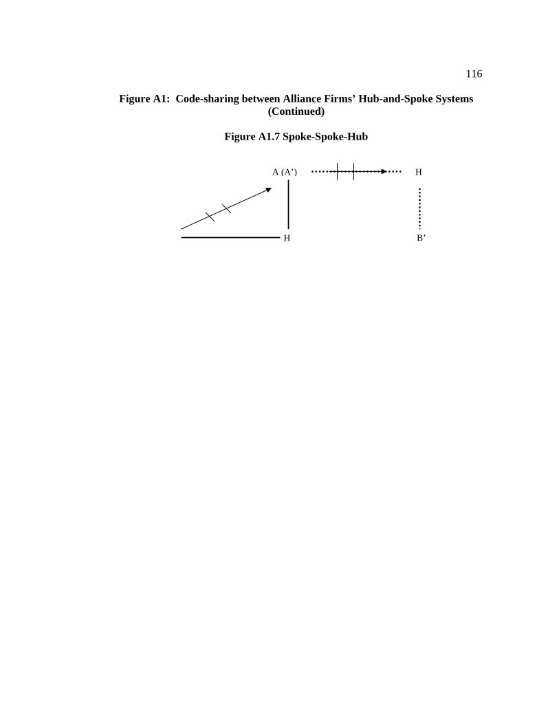
116
Figure A1: Code-sharing between Alliance Firms’ Hub-and-Spoke Systems (Continued)
Figure A1.7 Spoke-Spoke-Hub
H
B’
A (A’)
H
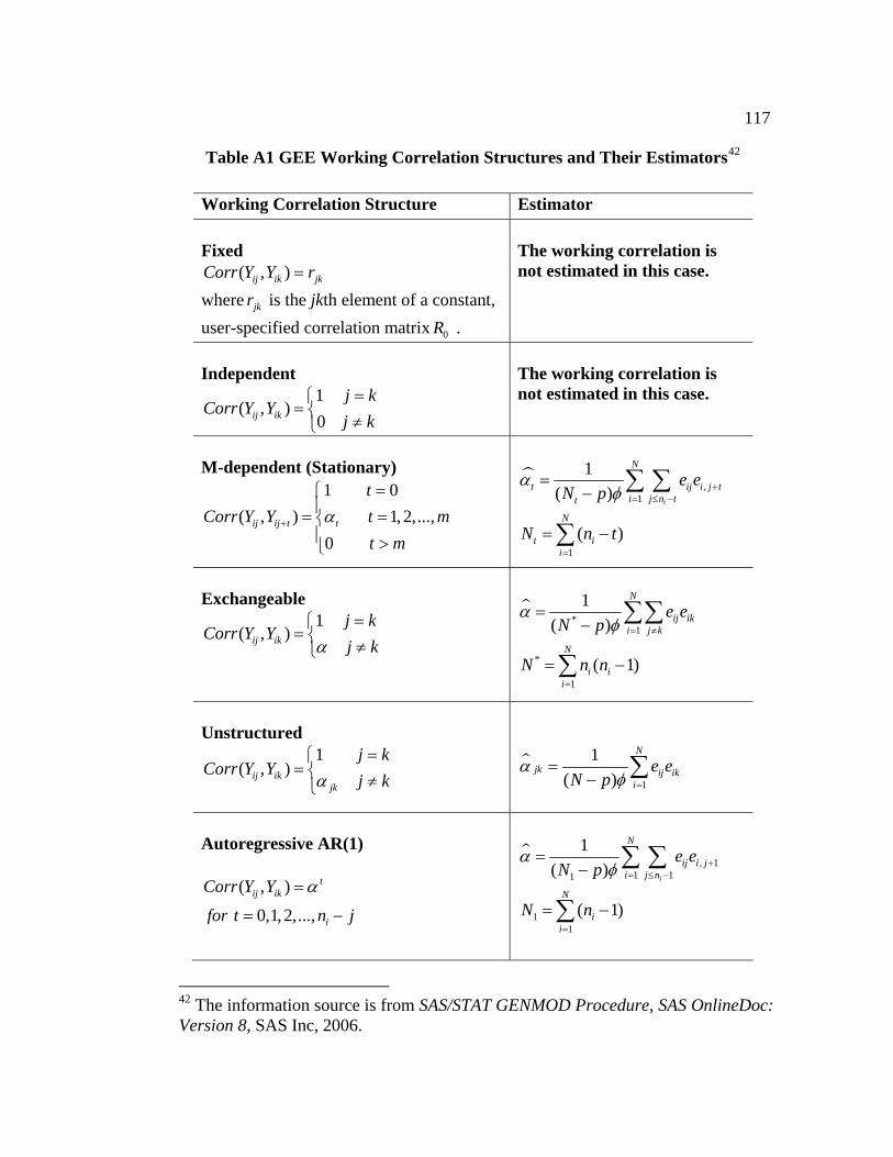
117
Table A1 GEE Working Correlation Structures and Their Estimators42
Working Correlation Structure Estimator Fixed
( , )ij ik jkCorr Y Y r= where jkr is the jkth element of a constant, user-specified correlation matrix 0R .
The working correlation is not estimated in this case.
Independent
The working correlation is not estimated in this case. 1
( , )0 ij ik
j kCorr Y Y
j k=⎧
= ⎨ ≠⎩
M-dependent (Stationary)
1 0( , ) 1, 2,...,
0 ij ij t t
tCorr Y Y t m
t mα+
=⎧⎪= =⎨⎪ >⎩
,1
1
1( )
( )
i
N
t ii j n tt
N
t ii
e eN p
N n t
αφ +
= ≤ −
=
=−
= −
∑ ∑
∑
j i j t
Exchangeable
42 The information source is from SAS/STAT GENMOD Procedure, SAS OnlineDoc: Version 8, SAS Inc, 2006.
1 ( , )
ij ik
j kCorr Y Y
j kα=⎧
= ⎨ ≠⎩
*1
*
1
1( )
( 1)
N
ij iki j k
N
i ii
e eN p
N n n
αφ = ≠
=
=−
= −
∑∑
∑
Unstructured
1 ( , )
ij ikjk
j kCorr Y Y
j kα=⎧
= ⎨ ≠⎩
1
1( )
N
jk ij iki
e eN p
αφ =
=− ∑
Autoregressive AR(1)
( , )
0,1, 2,...,
tij ik
i
Corr Y Y
for t n j
α=
= −
, 11 11
11
1( )
( 1)
i
N
ij i ji j n
N
ii
e eN p
N n
αφ +
= ≤ −
=
=−
= −
∑ ∑
∑
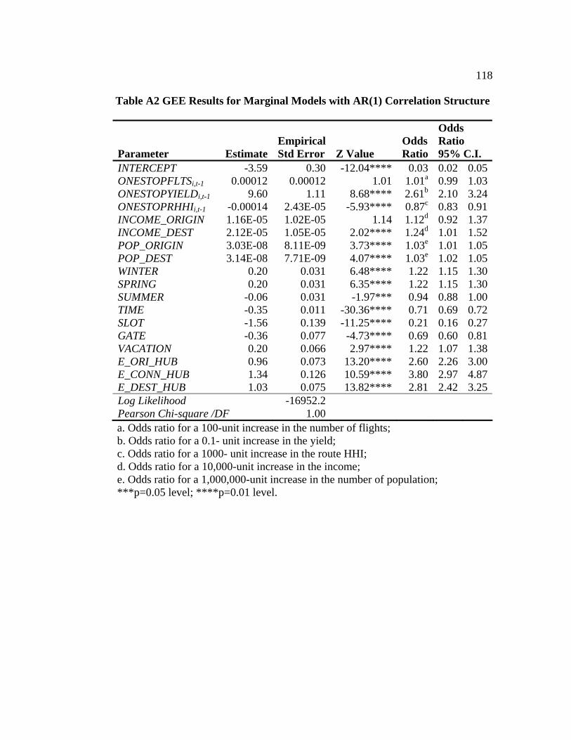
118
Table A2 GEE Results for Marginal Models with AR(1) Correlation Structure
Parameter EstimateEmpirical Std Error Z Value
Odds Ratio
Odds Ratio 95% C.I.
INTERCEPT -3.59 0.30 -12.04**** 0.03 0.02 0.05ONESTOPFLTSi,t-1 0.00012 0.00012 1.01 1.01a 0.99 1.03ONESTOPYIELDi,t-1 9.60 1.11 8.68**** 2.61b 2.10 3.24ONESTOPRHHIi,t-1 -0.00014 2.43E-05 -5.93**** 0.87c 0.83 0.91INCOME_ORIGIN 1.16E-05 1.02E-05 1.14 1.12d 0.92 1.37INCOME_DEST 2.12E-05 1.05E-05 2.02**** 1.24d 1.01 1.52POP_ORIGIN 3.03E-08 8.11E-09 3.73**** 1.03e 1.01 1.05POP_DEST 3.14E-08 7.71E-09 4.07**** 1.03e 1.02 1.05WINTER 0.20 0.031 6.48**** 1.22 1.15 1.30SPRING 0.20 0.031 6.35**** 1.22 1.15 1.30SUMMER -0.06 0.031 -1.97*** 0.94 0.88 1.00TIME -0.35 0.011 -30.36**** 0.71 0.69 0.72SLOT -1.56 0.139 -11.25**** 0.21 0.16 0.27GATE -0.36 0.077 -4.73**** 0.69 0.60 0.81VACATION 0.20 0.066 2.97**** 1.22 1.07 1.38E_ORI_HUB 0.96 0.073 13.20**** 2.60 2.26 3.00E_CONN_HUB 1.34 0.126 10.59**** 3.80 2.97 4.87E_DEST_HUB 1.03 0.075 13.82**** 2.81 2.42 3.25Log Likelihood -16952.2 Pearson Chi-square /DF 1.00
a. Odds ratio for a 100-unit increase in the number of flights; b. Odds ratio for a 0.1- unit increase in the yield; c. Odds ratio for a 1000- unit increase in the route HHI; d. Odds ratio for a 10,000-unit increase in the income; e. Odds ratio for a 1,000,000-unit increase in the number of population; ***p=0.05 level; ****p=0.01 level.
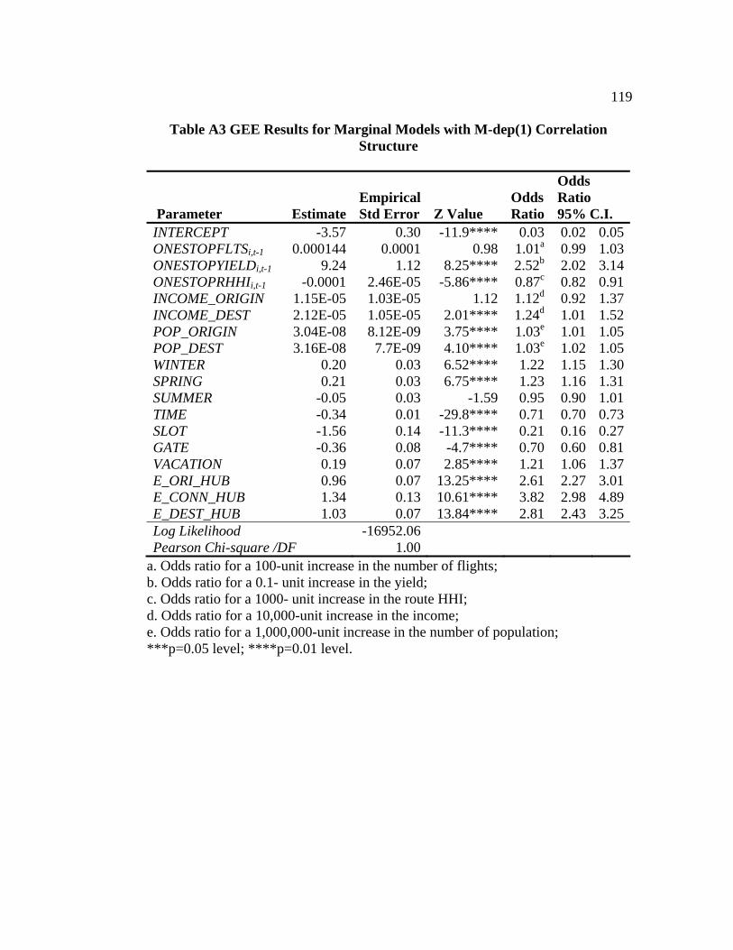
119
Table A3 GEE Results for Marginal Models with M-dep(1) Correlation Structure
Parameter EstimateEmpirical Std Error Z Value
Odds Ratio
Odds Ratio 95% C.I.
INTERCEPT -3.57 0.30 -11.9**** 0.03 0.02 0.05ONESTOPFLTSi,t-1 0.000144 0.0001 0.98 1.01a 0.99 1.03ONESTOPYIELDi,t-1 9.24 1.12 8.25**** 2.52b 2.02 3.14ONESTOPRHHIi,t-1 -0.0001 2.46E-05 -5.86**** 0.87c 0.82 0.91INCOME_ORIGIN 1.15E-05 1.03E-05 1.12 1.12d 0.92 1.37INCOME_DEST 2.12E-05 1.05E-05 2.01**** 1.24d 1.01 1.52POP_ORIGIN 3.04E-08 8.12E-09 3.75**** 1.03e 1.01 1.05POP_DEST 3.16E-08 7.7E-09 4.10**** 1.03e 1.02 1.05WINTER 0.20 0.03 6.52**** 1.22 1.15 1.30SPRING 0.21 0.03 6.75**** 1.23 1.16 1.31SUMMER -0.05 0.03 -1.59 0.95 0.90 1.01TIME -0.34 0.01 -29.8**** 0.71 0.70 0.73SLOT -1.56 0.14 -11.3**** 0.21 0.16 0.27GATE -0.36 0.08 -4.7**** 0.70 0.60 0.81VACATION 0.19 0.07 2.85**** 1.21 1.06 1.37E_ORI_HUB 0.96 0.07 13.25**** 2.61 2.27 3.01E_CONN_HUB 1.34 0.13 10.61**** 3.82 2.98 4.89E_DEST_HUB 1.03 0.07 13.84**** 2.81 2.43 3.25Log Likelihood -16952.06 Pearson Chi-square /DF 1.00
a. Odds ratio for a 100-unit increase in the number of flights; b. Odds ratio for a 0.1- unit increase in the yield; c. Odds ratio for a 1000- unit increase in the route HHI; d. Odds ratio for a 10,000-unit increase in the income; e. Odds ratio for a 1,000,000-unit increase in the number of population; ***p=0.05 level; ****p=0.01 level.
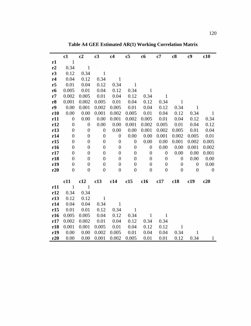
120
Table A4 GEE Estimated AR(1) Working Correlation Matrix
c1 c2 c3 c4 c5 c6 c7 c8 c9 c10 r1 1 r2 0.34 1 r3 0.12 0.34 1 r4 0.04 0.12 0.34 1 r5 0.01 0.04 0.12 0.34 1 r6 0.005 0.01 0.04 0.12 0.34 1 r7 0.002 0.005 0.01 0.04 0.12 0.34 1 r8 0.001 0.002 0.005 0.01 0.04 0.12 0.34 1 r9 0.00 0.001 0.002 0.005 0.01 0.04 0.12 0.34 1 r10 0.00 0.00 0.001 0.002 0.005 0.01 0.04 0.12 0.34 1r11 0 0.00 0.00 0.001 0.002 0.005 0.01 0.04 0.12 0.34r12 0 0 0.00 0.00 0.001 0.002 0.005 0.01 0.04 0.12r13 0 0 0 0.00 0.00 0.001 0.002 0.005 0.01 0.04r14 0 0 0 0 0.00 0.00 0.001 0.002 0.005 0.01r15 0 0 0 0 0 0.00 0.00 0.001 0.002 0.005r16 0 0 0 0 0 0 0.00 0.00 0.001 0.002r17 0 0 0 0 0 0 0 0.00 0.00 0.001r18 0 0 0 0 0 0 0 0 0.00 0.00r19 0 0 0 0 0 0 0 0 0 0.00r20 0 0 0 0 0 0 0 0 0 0 c11 c12 c13 c14 c15 c16 c17 c18 c19 c20 r11 1 1 r12 0.34 0.34 r13 0.12 0.12 1 r14 0.04 0.04 0.34 1 r15 0.01 0.01 0.12 0.34 1 r16 0.005 0.005 0.04 0.12 0.34 1 1 r17 0.002 0.002 0.01 0.04 0.12 0.34 0.34 r18 0.001 0.001 0.005 0.01 0.04 0.12 0.12 1 r19 0.00 0.00 0.002 0.005 0.01 0.04 0.04 0.34 1 r20 0.00 0.00 0.001 0.002 0.005 0.01 0.01 0.12 0.34 1
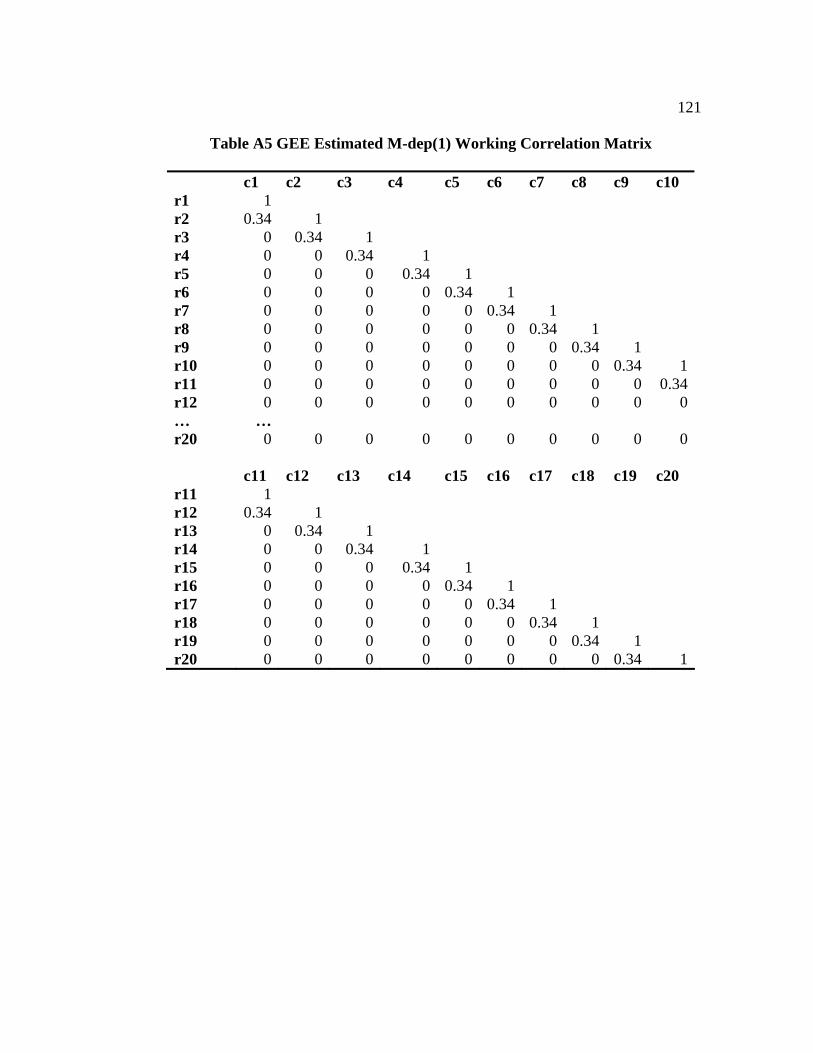
121
Table A5 GEE Estimated M-dep(1) Working Correlation Matrix
c1 c2 c3 c4 c5 c6 c7 c8 c9 c10 r1 1 r2 0.34 1 r3 0 0.34 1 r4 0 0 0.34 1 r5 0 0 0 0.34 1 r6 0 0 0 0 0.34 1 r7 0 0 0 0 0 0.34 1 r8 0 0 0 0 0 0 0.34 1 r9 0 0 0 0 0 0 0 0.34 1 r10 0 0 0 0 0 0 0 0 0.34 1r11 0 0 0 0 0 0 0 0 0 0.34r12 0 0 0 0 0 0 0 0 0 0… … r20 0 0 0 0 0 0 0 0 0 0 c11 c12 c13 c14 c15 c16 c17 c18 c19 c20 r11 1 r12 0.34 1 r13 0 0.34 1 r14 0 0 0.34 1 r15 0 0 0 0.34 1 r16 0 0 0 0 0.34 1 r17 0 0 0 0 0 0.34 1 r18 0 0 0 0 0 0 0.34 1 r19 0 0 0 0 0 0 0 0.34 1 r20 0 0 0 0 0 0 0 0 0.34 1
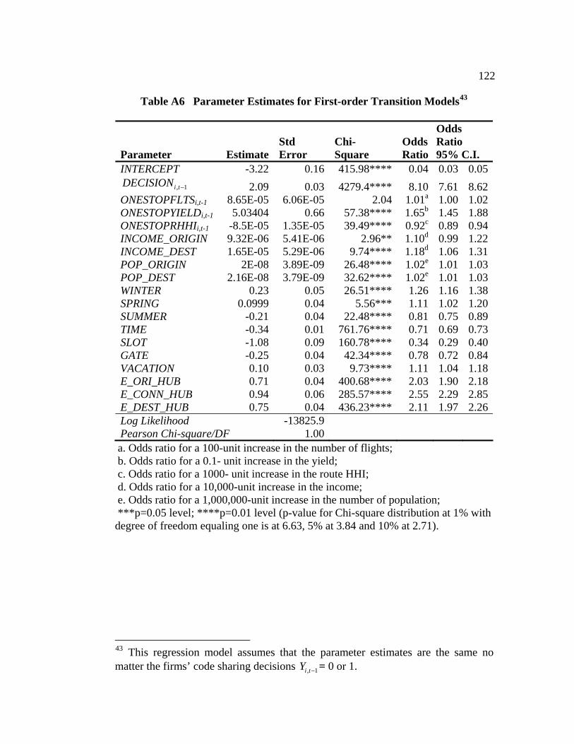
122
Table A6 Parameter Estimates for First-order Transition Models43
Parameter EstimateStd Error
Chi- Square
Odds Ratio
Odds Ratio 95% C.I.
INTERCEPT -3.22 0.16 415.98**** 0.04 0.03 0.05, 1i tDECISION − 2.09 0.03 4279.4**** 8.10 7.61 8.62
ONESTOPFLTSi,t-1 8.65E-05 6.06E-05 2.04 1.01a 1.00 1.02ONESTOPYIELDi,t-1 5.03404 0.66 57.38**** 1.65b 1.45 1.88ONESTOPRHHIi,t-1 -8.5E-05 1.35E-05 39.49**** 0.92c 0.89 0.94INCOME_ORIGIN 9.32E-06 5.41E-06 2.96** 1.10d 0.99 1.22INCOME_DEST 1.65E-05 5.29E-06 9.74**** 1.18d 1.06 1.31POP_ORIGIN 2E-08 3.89E-09 26.48**** 1.02e 1.01 1.03POP_DEST 2.16E-08 3.79E-09 32.62**** 1.02e 1.01 1.03WINTER 0.23 0.05 26.51**** 1.26 1.16 1.38SPRING 0.0999 0.04 5.56*** 1.11 1.02 1.20SUMMER -0.21 0.04 22.48**** 0.81 0.75 0.89TIME -0.34 0.01 761.76**** 0.71 0.69 0.73SLOT -1.08 0.09 160.78**** 0.34 0.29 0.40GATE -0.25 0.04 42.34**** 0.78 0.72 0.84VACATION 0.10 0.03 9.73**** 1.11 1.04 1.18E_ORI_HUB 0.71 0.04 400.68**** 2.03 1.90 2.18E_CONN_HUB 0.94 0.06 285.57**** 2.55 2.29 2.85E_DEST_HUB 0.75 0.04 436.23**** 2.11 1.97 2.26Log Likelihood -13825.9 Pearson Chi-square/DF 1.00
a. Odds ratio for a 100-unit increase in the number of flights; b. Odds ratio for a 0.1- unit increase in the yield; c. Odds ratio for a 1000- unit increase in the route HHI; d. Odds ratio for a 10,000-unit increase in the income; e. Odds ratio for a 1,000,000-unit increase in the number of population; ***p=0.05 level; ****p=0.01 level (p-value for Chi-square distribution at 1% with degree of freedom equaling one is at 6.63, 5% at 3.84 and 10% at 2.71).
43 This regression model assumes that the parameter estimates are the same no matter the firms’ code sharing decisions , 1i tY − = 0 or 1.