Embed Size (px)
Citation preview
EXTINCTION OF NEAR INFRARED SOLARRADIATION AS A MEANS FOR REMOTE
DETERMINATION OF ATMOSPHERIC WATER VAPOR.
Item Type text; Dissertation-Reproduction (electronic)
Authors THOMASON, LARRY WILLIS.
Publisher The University of Arizona.
Rights Copyright © is held by the author. Digital access to this materialis made possible by the University Libraries, University of Arizona.Further transmission, reproduction or presentation (such aspublic display or performance) of protected items is prohibitedexcept with permission of the author.
Download date 16/03/2022 11:24:49
Link to Item http://hdl.handle.net/10150/188078
INFORMATION TO USERS
This reproduction was made from a copy of a document sent to us for microfilming. While the most advanced technology has been used to photograph and reproduce this document, the quality of the reproduction is heavily dependent upon the quality of the material submitted.
The following explanation of techniques is provided to help clarify markings or notations which may appear on this reproduction.
1. The sign or "target" for pages apparently lacking from the document photographed is "Missing Page(s)". If it was possible to obtain the missing page(s) or section, they are spliced into the film along with adjacent pages. This may have necessitated cutting through an image and duplicating adjacent pages to assure complete con tinuity.
2. When an image on the film is obliterated with a round black mark, it is an indication of either blurred copy because of movement during exposure, duplicate copy, or copyrighted materials that should not have been filmed. For blurred pages, a good image of the page can be found in the adjacent frame. If copyrighted materials were deleted, a target note will appear listing the pages in the adjacent frame.
3. When a map, drawing or chart, etc., is part of the material being photographed, a definite method of "sectioning" the material has been followed. It is customary to begin filming at the upper left hand corner of a large sheet and to continue from left to right in equal sections with small overlaps. If necessary, sectioning is continued again-beginning below the first row and continuing on until complete.
4. For illustrations that cannot be satisfactorily reproduced hy xerographk means, photographic prints can be purchased at additional cost and inserted into your xerographic copy. These prints are available upon request from the Dissertations Customer Services Department.
5. Some pages in any document may have indistinct print. In all cases the best available copy has been filmed.
University Micrciilms
International 300 N. Zeeb Road Ann Arbor, MI48106
j
j
j
j
j
j
j
j
j
j
j
j
j
j
j
j
j
j
j
j
j
j
j
j
j
j
j
j
j
j
j
j
j
j
j
j
j
j
j
j
j
8529410
Thomason, Larry Willis
EXTINCTION OF NEAR INFRARED SOLAR RADIATION AS A MEANS FOR REMOTE DETERMINATION OF ATMOSPHERIC WATER VAPOR
The University of Arizona
University Microfilms
International 300 N. Zeeb Road, Ann Arbor, M148106
PH.D. 1985

EXTINCTION OF NEAR INFPJUtED SOLAR RADIATION
AS A MEANS FOR REMOTE DETERMINATION OF
ATMOSPHERIC WATER VAPOR
by
Larry Willis Thomason
A Dissertation Submitted to the Faculty of the
DEPARTMENT OF ATMOSPHERIC SCIENCE
In Partial Fulfillment of the Requirements For the Degree of
DOCTOR OF PHILOSOPHY
In the Graduate College
THE .UNIVERSITY OF ARIZONA
1 9 8 5
THE UNIVERSITY OF ARIZONA GRADUATE COLLEGE
As members of the Final Examinatior, Committee, we certify that we have read
the dissertation prepared by ____ ~L~a~r~r~y~W~i~l~l~i~s~T~h~o~m=a=s~o~n~ __________________ _
entitled _ ... El:;x~t=.:l.~·n~c~t::.:i~o~n~o~f--=.Nl.::e:.::a~r~I:.:n~f:.::r~a:.!:r..::e~d~S:.::o:,::::l~a:.!:r~Ra=d:.:=:i::::a;.::t~i::::o~ll:..:::a;:::s~a~M~e:::a~n:::s-=.fo=r __ _
Remote Determination of Atmospheric Water Vapor
and recommend that it be accepted as fulfilling the dissertation requirement
Date
Date )
/' t Date
Date
Final approval and acceptance of this dissertation is contingent upon the candidate's submission of the final copy of the dissertation to the Graduate College.
Date
STATEMENT BY AUTHOR
This dissertation has been submitted in partial fulfillment of requirements for an advanced degree at The University of Arizona and is deposited in the University Library to be made available to borrowers under rules of the Library.
Brief quotations from this dissertation are allowable without special permission, provided that accurate acknowledgment of source is made. Requests for permission for extended quotation from or reproduction of this manuscript in whole or in part may be granted by the head of the major department or the Dean of the Graduate College when in his or her judgment the proposed use of the material is in the interests of scholarship. In all other instances, however, permission must be obtained from the author.
ACKNOWLEDGMENTS
I wish to thank Dr. Ben Herman for his encouragement and
guidance in conduct of the research leading to this dissertation. I
also wish to thank Bill Chu of NASA-Langley for providing some of the
data used in Chapter IV.
I especially wish to acknowledge the patience and support that
my wife, Diane, has generously bestowed upon me over the last eight
years.
This research was supported by a grant from NOAA under contract
number NA80 RAD00065.
iii
TABLE OF CONTENTS
LIST OF ILLUSTRATIONS
LIST OF TABLES
ABSTRACT
CHAPTER
1. INTRODUCTION.
2. FORMULATION OF THE PROBLEM •
The General Band Transmission Function • • Transformation to Stieltjes Integral • Extension to Inhomogeneous Atmospheres •
3. THE RADIOMETRIC DETERMINATION OF PRECIPITABLE WATER
The Determination of k •.•.•••.• The Determination of k~(g) . • • • • The Determination of £ -l[T(u);u] • The Computation of Transmission Discussion • . • • . • • • .
4. THE RADIOMETRIC DETERMINATION OF STRATEOSPHERIC WATER VAPOR DISTRIBUTIONS . • • • . . • •
The Stratospheric Limb Scan Transmission Model The Determination of ku (g) • • • • • . . • • • • The Determination of the Verica1 Water Vapor
Distribution Discussion • • • • . •
5. SUMMARY AND CONCLUSIONS
LIST OF REFERENCES
iv
Page
v
ix
x
1
7
7 16 21
27
27 30 44 50 54
74
75 78
89 97
116
120
Figure
2.1.
2.2.
LIST OF ILLUSTRATIONS
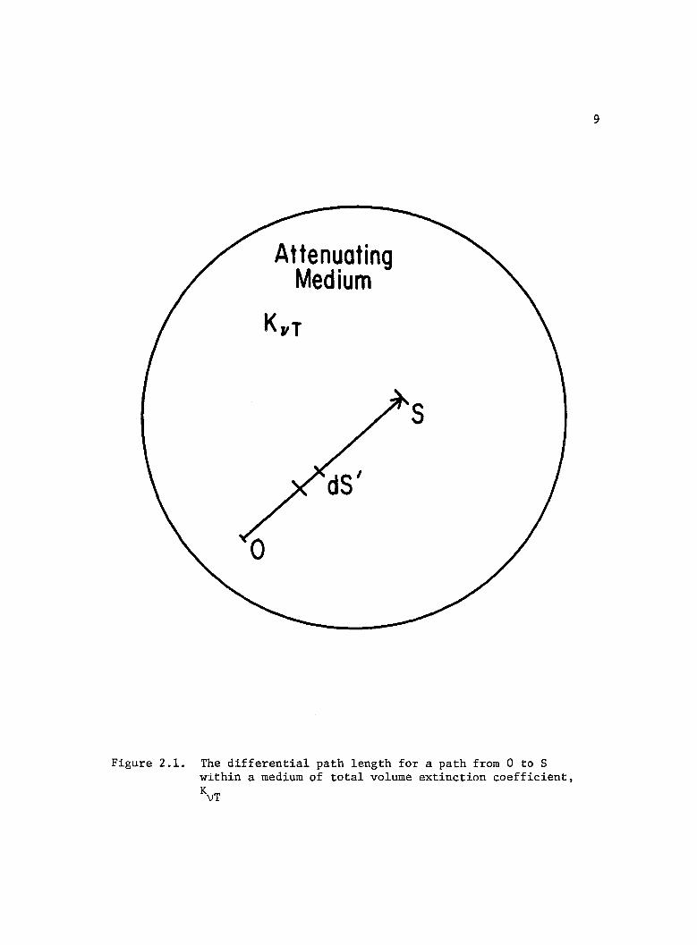
The differential path length for a path from 0 to S within a medium of total volume extinction coefficient, KVT • • • • • • • • • • • • • •
The true form (solid curve) and the histrogramic approximation to the product Iv(O)~(v) for the ground based radiometer's water vapor channel
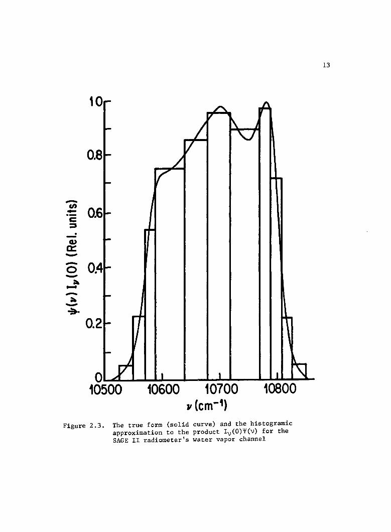
2.3. The true form (solid curve) and the histogramic approximation to the product Iv(O)~(v) for the
Page
9
12
SAGE II radiometer's water vapor channel. • • • • • •• 13
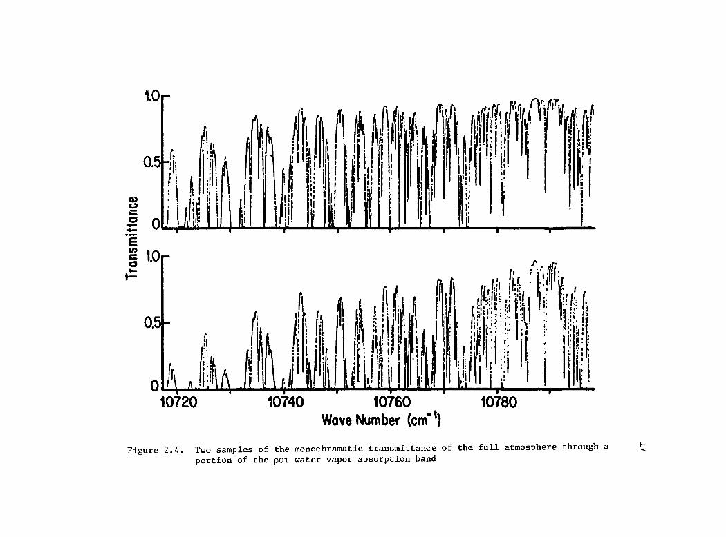
2.4. Two samples of the monochromatic transmittance of the full atmosphere through a portion of the POT water vapor absorption band • • • • • • • • •• 17
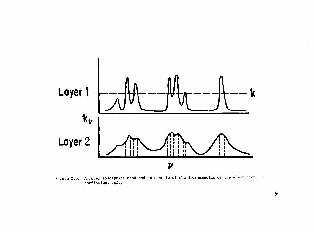
2.5. A model absorption band and an example of the incrementing of the absorption coefficient
2.6.
2.7.
axis •••
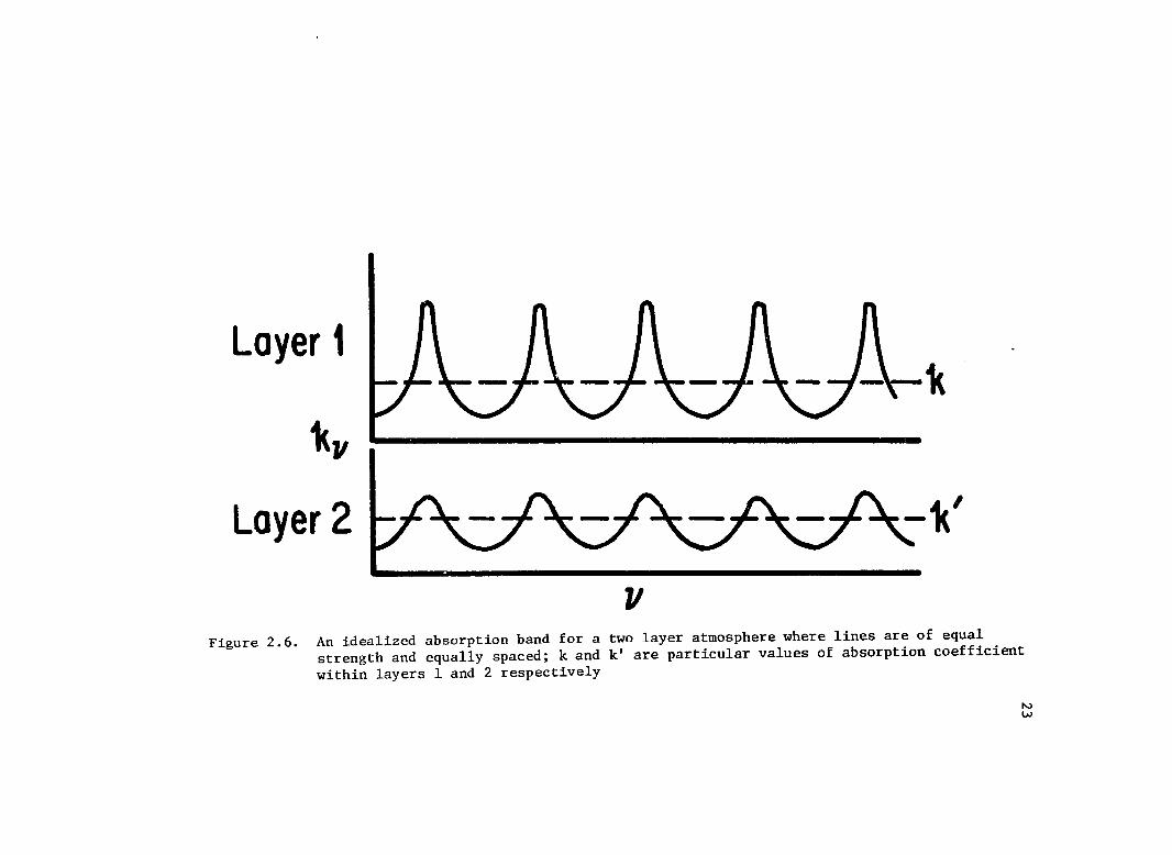
An idealized absorption band for a two layer atmosphere where lines are of equal strength and equally spaced; k and k' are particular values of absorption coefficient within layers 1 and 2 respectively . • • • • • • . • • • • •
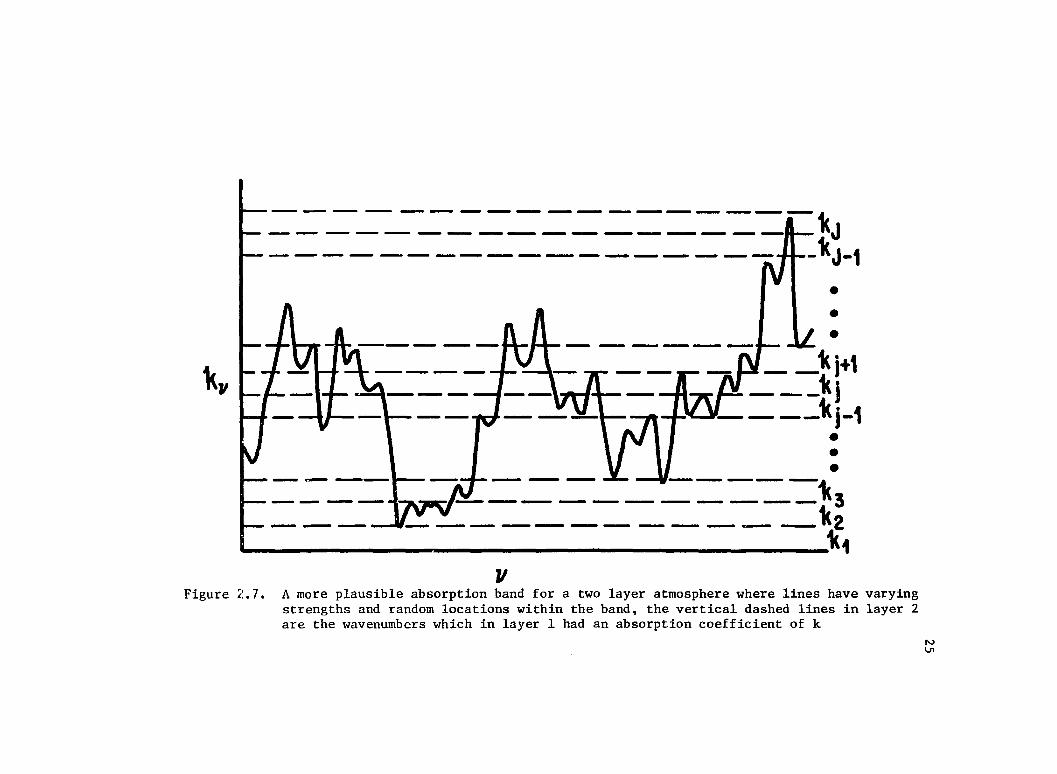
A more physically plausible absorption band for a two layer atmosphere where lines have varying strengths and random locations within the band, the vertical dashed lines in layer 2 are the wavenumbers which in layer 1 had an absorption coefficient of k • • • • • • • • • • • •
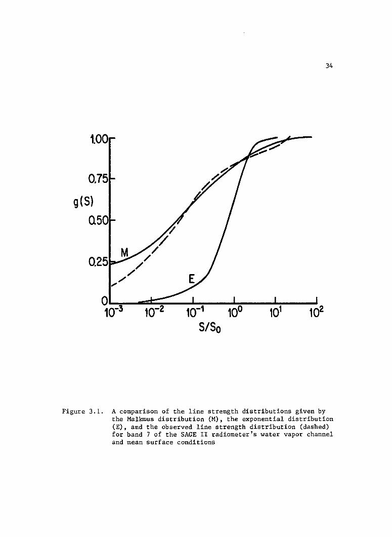
3.1. A comparison of the line strength distributions given by the Malkmus distribution (M), the exponential distribution (E), and the observed line strength distribution (dashed) for band 7 of the SAGE II radiometer's water vapor channel and mean surface conditions
v
18
23
25
34
LIST OF ILLUSTRATIONS--Continued
Figure
3.2. The ratio Wexp/WM as a function of x for the standard method (solid) and moment method
vi
Page
(dashed) of defining S' 0 and a. 't . . . . . . . . . . .. 43
3.3.
3.4.
3.5.
3.6
3.7.
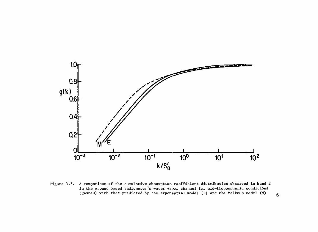
A comparison of the cumulative absorption coefficient distribution observed in band 2 in the ground based radiometer's water vapor channel for mid-tropospheric conditions (dasbed) with that predicted by the exponential model (E) and the Malkmus model (M) .••••••••
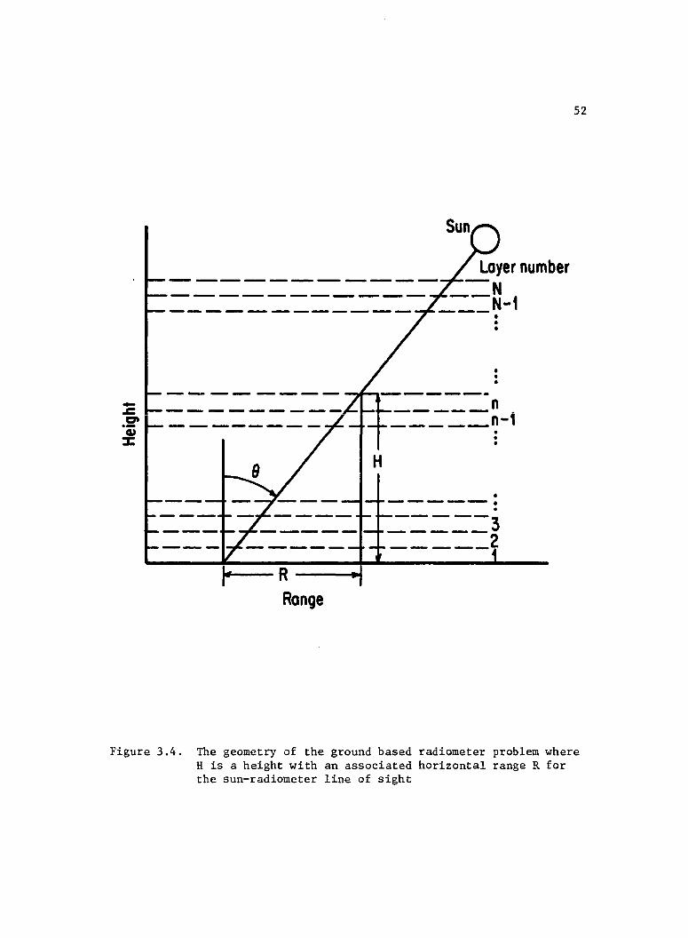
The geometry of the grcund based radiometer problem where H is a height with an associated horizontal range R for the sun-radiometer line of sight • • • • • • • • • • • • • • • • • . •
Effective optical depth as a function of mu for surface conditions of 2800 K and 950mb (I), 288°K and 940mb (II), and 305°K and 920bm (III)
The fraction of effective optical depth, L , and precipitable water originatin~ below a gIven height for mean atmospheric conditions
The local powers Pa.(x), P (x), and Pa.(x)/P (x) as functions of x .• ~ ••..•••• u ••
3.8. The correlation, p, of the k(v) function for certain reference layers with the k(v) for the layers above the reference layer; the calculation was performed for band 3 of the ground based radiometer's water vapor channel and standard
49
52
56
57
62
atmospheric conditions • . . • • • . • •• •• . •. 65
3.9a. The value of G for selected reference layers as a function of the companion layer for band 2 of the ground based radiometer's water vapor channel and standard atmospheric conditions
3.9b. The value of G for selected reference layers as a function of the companion layer for band 7 of the SAGE II radiometer's water vapor channel and standard atmospheric conditions . . . • . . . . .
67
68
Figure
3.10.
LIST OF ILLUSTRATIONS--Continued
The dependence of the error introduced by the assumption of complete rank preservation on u and G • . • . • . • •. •• • • . • •
3.11. A comparison of radiometric and radiosonde determinations of precipitable water; the solid line is curve II from Figure 3.5 and the data points are measured water vapor effective optical depth versus radiosonde precipitable water times the airmass of the radiometer measurement
4.1. The geometry of a SAGE II measurement with a tangent height of Z ........•.
m
4.2. The dependence of the Lorentz, Doppler and Voight half widths on height for standard atmospheric
4.3.
4.4.
conditions
The fractional error, £u' in the estimation of the path water vapor amount, u, due to the assumption that the Voight transmission function has the same form as the Ma1kmus transmission function. Eu is shown for band 7 (10,720-10,770 cm-1) of the SAGE II radiometer and for selected heights • . • • •
The fractional error, Eu' in the estimation of the path wat£r vapor amount, u, due to the assumption that the Voight transmission function has the same form as the Ma1kmus transmission function. Eu is shown as a function of height for the total interval and selected water vapor amounts • • • • •
4.5. The model g(h) (dashed) and the true g(h) (solid) for band 7 of the SAGE II radiometer and mid-
4.6.
4.7.
stratospheric conditions
The effective optical depth as a function of total path water vapor, u(ZT)' for selected tangent heights and standard atmospheric conditions • • . •
The local power P (ZT) as a function of u(ZT) 10r selected tangen~ heights and standard atmospheric condi tions • • • • • . . . • . • . • . • . • • •
vii
Page
70
71
76
79
84
85
87
91
92
viii
LIST OF ILLUSTRATIONS--Continued
Figure Page
4.8. Iterative solutions to the case I set of measured effective optical depths for Cleveland, Ohio 96
4.9. The function gL(l) as a function of height for selected tangent heights and standard atmospheric conditions • •• • • • • • • • • • • • 99
4.10. The fractional uncertainty, £q, in the estimated vertical water vapor distribution resulting from random measurement errors that have a standard deviation of 10% in u(ZT) at any given height • • • . • • • . • • • • • • • • • • • • • 102
4.11. The fractional uncertainty, £q, in the estimated vertical water vapor distribution resulting from a locally systematic error in the estimated verti-cal temperature field • • • • • • • • • • 105
4.12. The fractional uncertainty, £1' in the estimated vertical water vapor distribution resulting from the uncertainty in the specification of a'v (solid) and from all significant sources of model uncertainty (dashed) • •• • . • • •
4.l3a. Case I solution q3 (solid) and the NASA-Langley solution (dashed) • • • • • • .
4.l3b. Case II solution q3 (solid) and the NASA-Langley solution (dashed) •••• • • • • . •
4.l3c. Case III solution q3 (solid) and the NASA-Langley solution (dashed) • • • • • • • • • • .
4.14. The fractional uncertaintY'£q' due to random measurement errors as estimated by NASA-Langley for cases I, II, and III •.••••••.••
106
109
110
III
112
LIST OF TABLES
Table
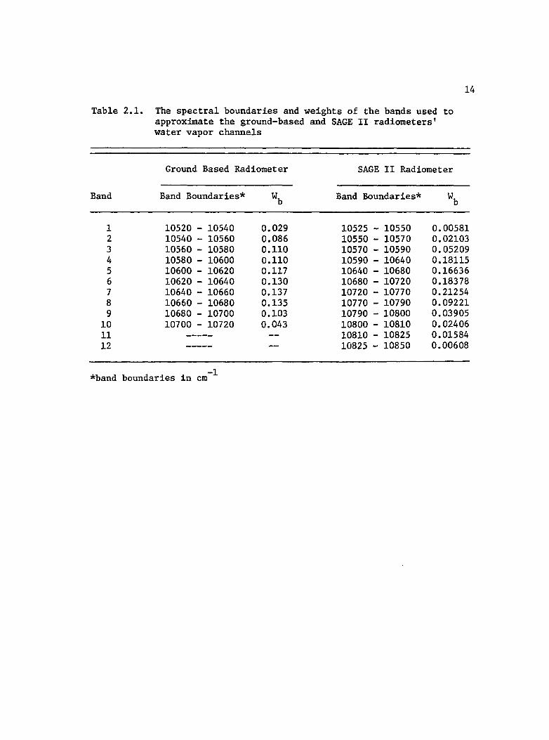
2.1. The spectral boundaries and weights of the bands used to approximate the ground-based and SAGE II radio-
Page
meters' water vapor channels. • • • • • • • • •• 14
3.1. Comparison of equivalent Lorentz line widths as determined from the moments of the absorption coefficient distribution for band 3 of the ground based radiometer and mean surface conditions • • • • • • • • • • • • • 59
4.1. The normalized correlation coefficient between the solution elements qn and qn+6n as a function of the separation between the layers nand n + 6n •..•• 103
ix
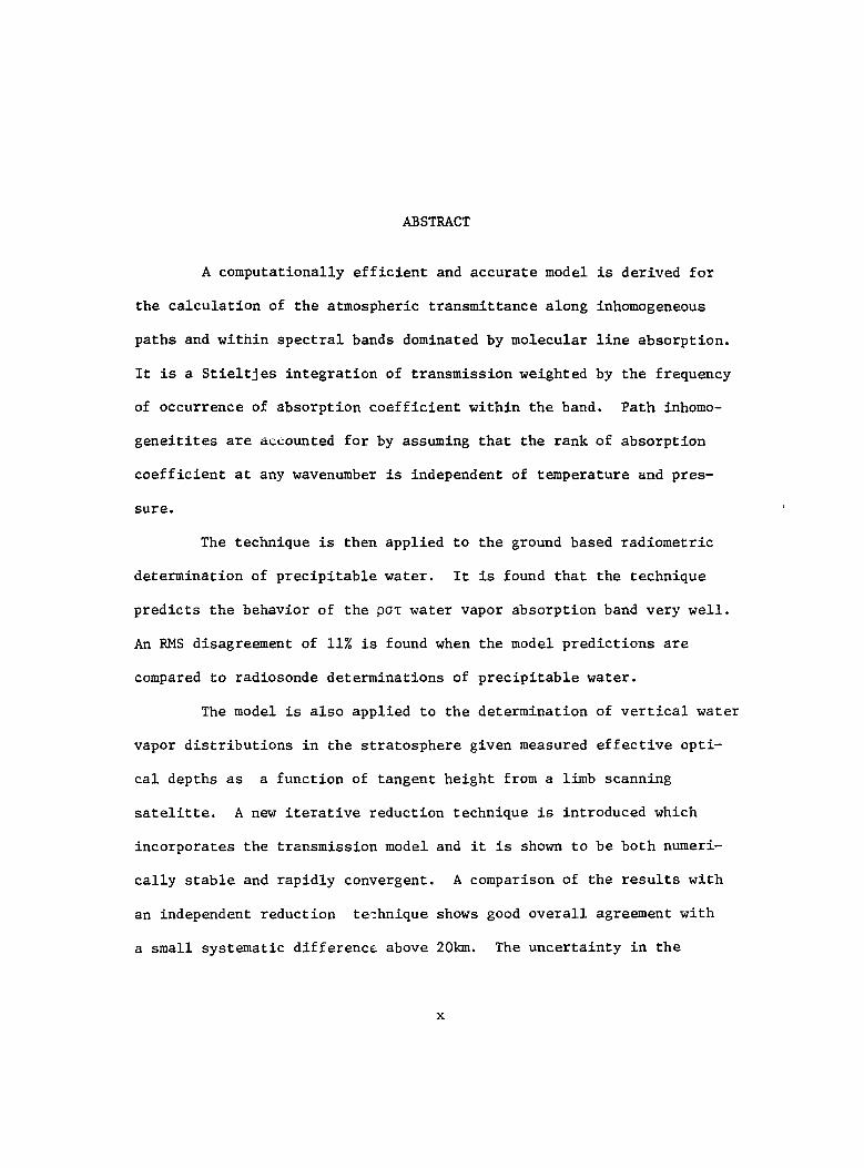
ABSTRACT
A computationally efficient and accurate model is derived for
the calculation of the atmospheric transmittance along inhomogeneous
paths and within spectral bands dominated by molecular line absorption.
It is a Stieltjes integration of transmission weighted by the frequency
of occurrence of absorption coefficient within the band. Path inhomo
geneitites are accounted for by assuming that the rank of absorption
coefficient at any wavenumber is independent of temperature and pres
sure.
The technique is then applied to the ground based radiometric
determination of precipitable water. It is found that the technique
predicts the behavior of the pOT water vapor absorption band very well.
An RMS disagreement of 11% is found when the model predictions are
compared to radiosonde determinations of precipitable water.
The model is also applied to the determination of vertical water
vapor distributions in the stratosphere given measured effective opti
cal depths as a function of tangent height from a limb scanning
satelitte. A new iterative reduction technique is introduced which
incorporates the transmission model and it is shown to be both numeri
cally stable and rapidly convergent. A comparison of the results with
an independent reduction te~hnique shows good overall agreement with
a small systematic difference above 20km. The uncertainty in the
x
measurements, which yields solution uncertainties on the order of
30%, renders this systematic difference unimportant.
xi
CHAPTER 1
INTRODUCTION
Trace gas constituents in the terrestrial atmosphere
frequently assume a greater importance than their relative abundances
would imply due to their role in one or more of the physical processes
occuring within the atmosphere. The hydroxyl radical is of great
importance in atmospheric chemical reactions yet has an abundance of
7 +3 only about 10 molecules/cm (Heicklen s 1976, p. 293). Carbon dioxide
with an abundance of little more than 300ppm is of great importance in
radiative heat transport. But of all of the trace gases, it is water
vapor that assumes the greatest importance because of the major role
it plays in many of the physical processes in the atmosphere. Beyond
it's obvious and extraordinary role in precipitation, water vapor also
plays a significant role in atmospheric chemical processes (Heicklen,
1976, pp. 83-97), radiative heat transport (Rodgers and Walshaw, 1966)
and latent heat transport (Chou and Atlas, 1982).
Because of water vapor's importance, it has long been con-
sidered cri~ical to a complete description of the state of the atmo-
sphere that the amount of water vapor to be specified. The in situ
measurement of water vapor also known as hygrometry has a long history
and may be traced to 1500 when Leonardo DaVinci experimented with a
simple hygrometer. A complete discussion of the theory of hygrometry
1
may be found in Spencer-Gregory and Rourke (1957) including a
discussion of most of the common instruments in use today.
2
One of the major difficulties with in situ measurements is that
water vapor is not well mixed in the atmosphere and may vary rapidly
both horizontally and vertically. Radiosondes may be used to determine
the vertical distribution of water vapor above a release site and with
data from a network of such sites, it is possible to derive an approx
imate three-dimensional distribution of water vapor, but the density
of the launch sites and frequency of the releases are limited by cost
considerations. Furthermore, such launch sites are virtually non
existant over vast oceanic areas covering about three quarters of the
globe. Water vapor amounts as determined by radiosondes have a rea
sonable degree of reliability over the bulk of the troposphere. At
higher altitudes, however, where the water vapor density is low, the
reliability of the simple hygrometer used in the radiosonde decreases
significantly and above the tropopause usually no useful data is re
trieved. In this work, two problems will be considered for which the
radiosonde and the radiosonde network are not adequate.
The first problem is the real time monitoring of precipitable
water which is the total mass of water vapor in a unit, vertically
oriented, column of the atmosphere. The reason that this is of
interest is because the probability of summer airmass thunderstorms
in the Tucson area is closely related to the precipitable water. The
mesoscale dynamics of the summer monsoon permit the rapid fluctuation
of preCipitable water during the course of the day. Therefore the
precipitable water inferred from the morning radiosonde sounding,
launched at 0500 MST, may not be valid by afternoon when thunderstorm
activity would be expected. So by monitoring precipitable water, it
may be possible to improve the predictability of afternoon thunder
storms.
The second problem is the determination of stratospheric ver
tical water vapor profiles and ultimately the construction of three
dimensional distributions of water vapor within the stratosphere.
There is interest in this because little is known about the climatol
ogy of the distribution of water vapor in the stratosphere. It is
also possible, given histories of the three dimensional distribution
of water vapor, to infer stratospheric circulation patterns and the
rate of production of H20 in the upper stratosphere associated with
methane photodisassociation.
A technique which may be employed to solve these problems is
passive remote sensing. Remote sensing is the determination of some
property of the atmosphere via a signal, measured some distance from
the source of the signal. Passive remote sensing makes use of
naturally occurring radiative field.s, that is, ones which are not
anthrpogenic. Among the approaches that have been used to passively
determine atmospheric water vapor amounts are multichannel microwave
and infrared radiometers which make use of the dependence of the
emissivity of water vapor on frequency and temperature to determine
water vapor profiles (Staelin et al., 1976; Russell et al., 1984).
Another technique, and the one of interest here, is the use of a
3
single spectral determination of the transmission of solar radiation
to infer the water vapor amount along a path from the sun to a radio
meter that is directly observing the sun. The assertion in this
technique is that if a spectral channel is chosen to lie within a
region in which attenuation is dominated by water vapor absorption
lines then it is possible to infer the path water vapor amount given
a measured water vapor optical depth.
While the problem of equating water vapor optical depth with
water vapor amount initially seems to be a straight forward problem,
it turns out to be quite complicated. The main problem in solving
this equivalency is that the mass absorption coefficient is a highiy
complicated function of wavenumber within an absorption band and it
is also a strong function of temperature and pressure thus making it
difficult to adequately determine the expected water vapor transmis
sion for a given set of conditions. Various approximate techniques
have been developed and used over the past ten or twenty years and
among these are numerically fitting point determinations of trans
mission as a function of absorber amount (Liou, 1974)s }~boratory
calibration of the radiometer (Tomasi et a1., 1983), and the fourier
transform method (Mankin, 1979). Herein, a new approach to this
problem is developed which satisfactorily meets the requirements
placed upon it, that is, it must be computationally efficient and
accurate to the degree that compared to measurement errors it does
not itself represent a significant degradation in the water vapor
4
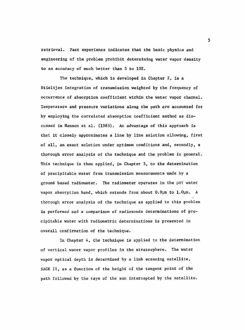
retrieval. Past experience indicates that the basic physics and
engineering of the problem prohibit determining water vapor density
to an accuracy of much better than 5 to 10%.
The technique, which is developed in Chapter 2, is a
Stieltjes integration of transmission weighted by the frequency of
occurrence of absorption coefficient within the water vapor channel.
Temperature and pressure variations along the path are accounted for
by employing the correlated absorption coefficient method as dis
cussed in Hansen et al. (1983). An advantage of this approach is
that it closely approximates a line by line solution allowing, first
of all, an exact solution under optimum conditions and, secondly, a
thorough error analysis of the technique and the problem in general.
This technique is then applied, in Chapter 3, to the determination
of precipitable water from transmission measurements made by a
ground based radiometer. The radiometer operates in the POT water
vapor absorption band, which extends from about 0.9~m to l.~m. A
thorough error analysis of the technique as applied to this problem
is performed and a comparison of radiosonde determinations of pre
cipitable water with radiometric determinations is presented in
overall confirmation of the technique.
In Chapter 4, the technique is a~plied to the determination
of vertical water vapor profiles in the stratosphere. The water
vapor optical depth is determined by a limb scanning satellite,
SAGE II, as a function of the height of the tangent point of the
path followed by the rays of the sun intercepted by the satellite.
5
A new iterative inversion of the water vapor optical depths to water
vapor mixing ratio as a function of height is developed and is shown
to be both numerically stable and rapidly convergent. A complete
error analysis of the inversion technique and comparisons with an
independent reduction technique are presented and show that the
precision of the approach is significantly better than the quality of
the data provided by SAGE II.
Chapter 5 presents some general discussion and conclusions
about the o'verall utility of the technique and its applicability to
the problems presented within this dissertation. Also included are
some suggestions for improving the technique, particularly for
stratospheric applications.
6
CHAPTER 2
FORMULATION OF THE PROBLEM
The transport of radiant energy through a medium in
thermocynamic equilibrium is governed by the Equ,ation of Radiative
Transfer which is most fundamentally a statement of the conservation
of energy. Solutions to this equation can be either for a single
wavelength, as is common when studying light scattering by aerosols,
or for a band, or interval of wavelength, as is most often of interest
when considering radiative transfer in spectral regions dominated by
molecular line absorption.
In this chapter, starting from the Equation of Radiative
Transfer, a general form of the band transmission function will be
derived that is valid for an attenuating atmosphere with no internal
sources of radiant energy. Limiting consideration to attenuation by
molecular line absorption, the general band transmission function is
transformed to a Stieltjes integral. The steps necessary to incor
porate the correlated absorption coefficient assumption for paths
along which temperature and pressure are allowed to freely vary, are
also shown.
The General Band Transmission Function
Most solutions to radiative transport problems begin with the
Equation of Radiative Transfer because it expresses the fundamental
7
8
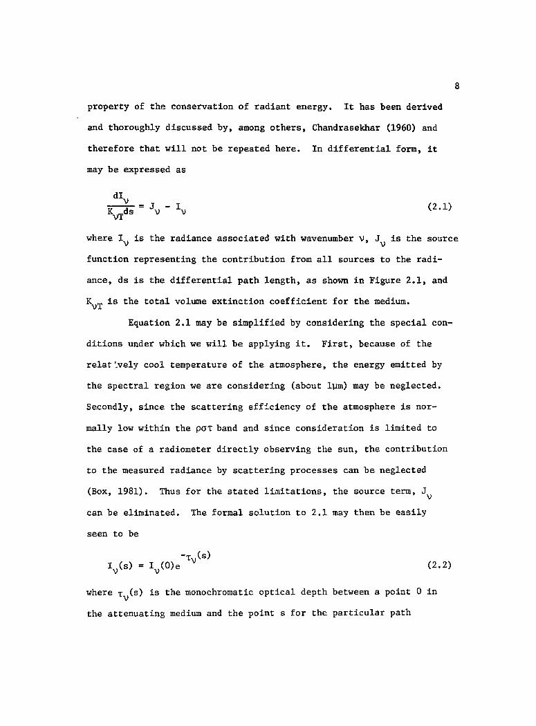
property of the c.onservation of radiant energy. It has been derived
and thoroughly discussed by, among others, Chandrasekhar (1960) and
therefore that will not be repeated here. In differential form, it
may be expressed as
(2.1)
where Iv is the radiance associated with wavenumber v, Jv
is the source
function representing the contribution from all sources to the radi-
ance, ds is the differential path length, as shown in Figure 2.1, and
KVT is the total volume extinction coefficient for the medium.
Equation 2.1 may be simplified by considering the special con-
ditions under which we will be applying it. First, because of the
relat:vely cool temperature of the atmosphere, the energy emitted by
the spectral region we are considering (about l~m) may be neglected.
Secondly, since the scattering efficiency of the atmosphere is nor-
mally low within the POT band and since consideration is limited to
the case of a radiometer directly observing the sun, the contribution
to the measured radiance by scattering processes can be neglected
(Box, 1981). Thus for the stated limitations, the source term, J v
can be eliminated. The formal solution to 2.1 may then be easily
seen to be
(2.2)
where LV(S) is the monochromatic optical depth between a point 0 in
the attenuating medium and the point s for the particular path
Attenuating Medium
5
Figure 2.1. The differential path length for a path from 0 to S within a medium of total volume extinction coefficient,
KVT
9
10
followed. Iv(O) is the radiance of wavenumber incident at the
point along the path where s is zero. Formally, the monochromatic
optical depth may be expressed as
s f K (s')ds' o vT
(2.3)
Equation 2.2 is the well known Beer's Law and, physically, it expresses
the fact that for the conditions described above, the'radiance mea-
sured in any direction is equal to the incident radiance in that di
rection reduced by a factor of e-Lv(s).
In extending Beer's Law to an interval in wavenumber, there is
a temptation to express Equation 2.2 as
- --L I(s) = 1(0) (2.4)
where the bar superscript is indicative of averaging the quantity over
some interval in wavenumber. But, it has been shown (Thomason et al.,
1982) that even in cases where the monochromatic optical depth is not
a very strong function of wavenumber, this is not a satisfactory ap-
proach as it can yield sizeable errors for even fairly narrow inter-
valse It is necessary, therefore, to consider an integral form of
Beer's Law, including a filter spectral response for the radiometer,
in order t~ correctly determine the measured radiance. Equation 2.2
is then expressed as
(2.5)
where 6v is the band's width in wavenumber, and ~(v) is the radio-
meter's spectral filter response. A general transmission function
can now be phrased by dividing Equation 2.5 by 1(0), which yields
11
-T (S) T(s) = l(s)/I(O) = 16vlv(0)~(v)e v dvI16vIv(0)~(V)dy (2.6)
The transmission function, T(s), will have a value of 1.0 when s is
zero and decreases monotonically toward zero with increasing s.
Equation 2.6 can be simplified by dividing the inter'lal into
small bands within which the product Iv(O)~(V) may be considered con
stant resulting in an approximate general transmission function that
is the weighted summation of the band transmission functions; that is
B
T(s) = b~l WbTb(s) (2.7)
where B is the number of bands and Wb is the individual band weighting
which is given by
where 6vb is the band width in wavenumber. Tb(s) is the band transmis
sion function and is formally expressed as
(2.9)
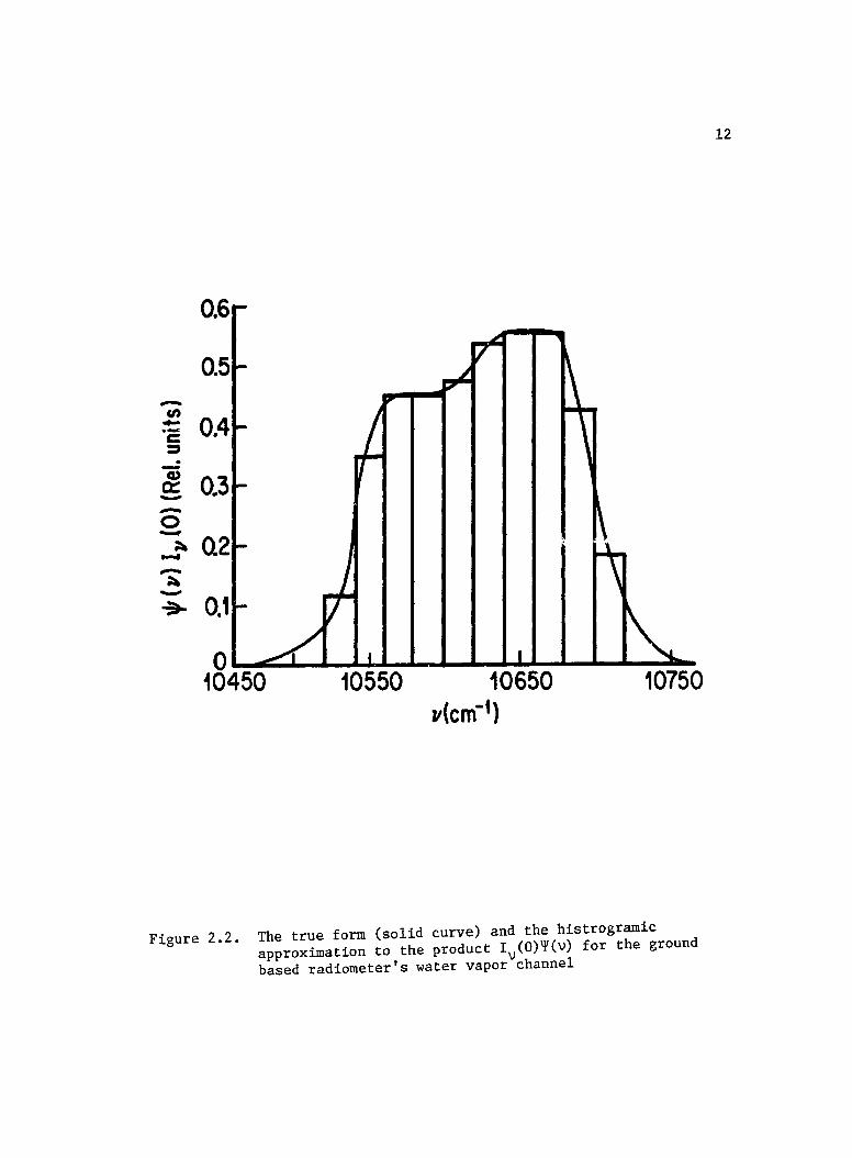
In the pOT band, Iv(O) is very nearly constant and the variations in
I (O)~(v) are due almost entirely to the variations of the filter V
function across the band. Figures 2.2 and 2.3 show the approxima-
tions for 1v(0)~(v) that were used in determining the band transmis
sion for the ground based radiometer and the SAGE II radiometer,
respectively. Table 2.1 lists the weights that were used for the
bands for each radiometer.
-tn -·c ::J .
Q) 0:: --o -~ .... -~ -
184!i:5~O :;....&..~1±05~5~O..L.....JL-L~1 O~6~5~O .L..J~-1.:::t07""50 v(cm-t)
Figure 2.2. The true form (solid curve) and the histrogramic approximation to the product Iv(O)~(V) for the ground based radiometer's water vapor channel
12
~
en ... --c ::s . -CL)
0:: -~
o -~ ..... ~
~ -~.
10600 10700 10800 If (cm-1)
Figure 2.3. The true form (solid curve) and the histogramic approximation to the product Iv(O)~(v) for the SAGE II radiometer's water vapor channel
13
14
Table 2.1. The spectral boundaries and weights of the bands used to approximate the ground-based and SAGE II radiometers' water vapor channels
Ground Based Radiometer SAGE II Radiometer
Band Band Boundaries* Wb Band Boundaries* Wb
1 10520 - 10540 0.029 10525 - 10550 0.00581 2 10540 - 10560 0.086 10550 - 10570 0.02103 3 10560 - 10580 0.110 10570 - 10590 0.05209 4 10580 - 10600 0.110 10590 - 10640 0.18115 5 10600 - 10620 0.117 10640 - 10680 0.16636 6 10620 - 10640 0.130 10680 - 10720 0.18378 7 10640 - 10660 0.137 10720 - 10770 0.21254 8 10660 - 10680 0.135 10770 - 10790 0.09221 9 10680 - 10700 0.103 10790 - 10800 0.03905
10 10700 - 10720 0.043 10800 - 10810 0.02406 11 10810 - 10825 0.01584 12 10825 - 10850 0.00608
*band boundaries in cm -1
15
At most wavenumbers, the monochromatic optical depth has
components from aerosol and molecular scattering and absorption by
aerosol and various gases. In the pOT band, in addition to water
vapor absorption, there are small but non-negligible contributions to
the monochromatic optical depth by scattering, aerosol and molecular,
and by absorption due to ozone. In order to determine a water vapor
amount from a single transmission measurement it is necessary to be
able to remove the effect of the non-water vapor attenuators. There
are techniques to permit this and, as they are not of interest herein,
it will be assumed they have been performed and limit consideration to
the attenuative effects of water vapor only. It is important to remem-
ber, however, that errors arising because of the neglect of these non-
water vapor attenuation components will have an important effect on
the quality of the water vapor determination made from any given mea-
surement.
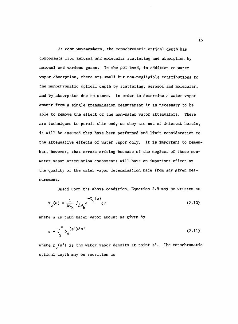
Based upon the above condition, Equation 2.9 may be written as
where u is path water vapor amount as given by
u S (s')ds'
f Pv o
(2.10)
(2.11)
where PoJ(s') is the water vapor density at point s'. The monochromatic
optical depth may be rewritten as
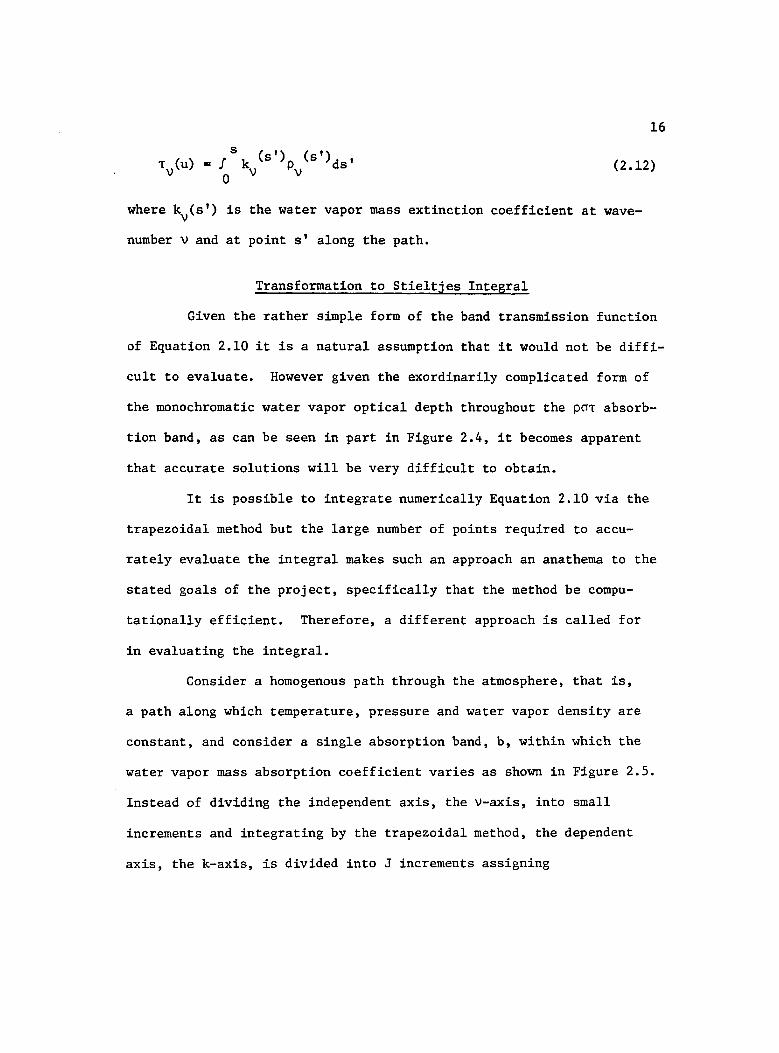
16
T (U) = f s k (s')p (s')ds' v a v v (2.12)
where kv(s') is the water vapor mass extinction coefficient at wave
number V and at point s' along the path.
Transformation to Stieltjes Integral
Given the rather simple form of the band transmission function
of Equation 2.10 it is a natural assumption that it would not be diffi-
cult to evaluate. However given the exordinarily complicated form of
the monochromatic water vapor optical depth throughout the POT absorb-
tion band, as can be seen in part in Figure 2.4, it becomes apparent
that accurate solutions will be very difficult to obtain.
It is possible to integrate numerically Equation 2.10 via the
trapezoidal method but the large number of points required to accu-
rately evaluate the integral makes such an approach an anathema to the
stated goals of the project, specifically that the method be compu-
tationally efficient. Therefore, a different approach is called for
in evaluating the integral.
Consider a homogenous path through the atmosphere, that is,
a path along which temperature, pressure and water vapor density are
constant, and consider a single absorption band, b, within which the
water vapor mass absorption coefficient varies as shown in Figure 2.5.
Instead of dividing the independent axis, the v-axis, into small
increments and integrating by the trapezoidal method, the dependent
axis, the k-axis, is divided into J increments assigning
Q) (.) c c --E
1.0
o.
~ 1.0 c ~
I-
o.
0 1111
10720
~"Ill lJ Ii i'1~ I! P 1 'l~ lUI I" 1 ~~ ,: ~ i'~. f!I-~ I Will \- r I~ ~ll~ Ii I I: I lh Iii f ! I f II I ! I I II , . ~ . i: ': i , n I :' I • I I' I ',' . I . i " I! I" r I! I 'I'"~ ~ ~ ,; 1'1 : 1"1 'I'll': I I I: :: . I, "II
, :1, ii/II,. I; Ill' 11 II~'! ~ r; I' I~f I i I' 1\ ,I II I I 5 ,I. • I ! II r I: I II' . '
10760 Wave Number (cm-')
10780
Figure 2.4. Two samples of the monochramatic transmittance of the full atmosphere through a portion of the POT water vapor absorption band
...... -..J
Layer 1 --\
1<11
Layer 2
71 Figure 2.5. A model absorption band and an example of the incrementing of the absorption
coefficient axis.
.... 00
19
characteristic values of water vapor absorption coefficient to each
increment, as shown in Figure 2.5. Now if Equation 2.10 is integrated
only over the domain of wavenumbers within the band with water vapor
mass absorption coefficients lying within the jth increment, 6v(j) and
the homogeneity condition previously stated is invoked, Equation 2.10
may be rewritten as
or
-k.u T.(u) - ~ f e J dv
J - 6vb 6v{j)
-k u e j
Tj(U) = -6- f d vb 6v(j) v
(2.13)
(2.14)
In this equation, T.(u) is the transmissivity associated with an abJ
sorption of value k. and absorber amount u weighted by the "probabilJ
ity" of any wavenumber within the band being associated with the jth
increment in absorption coefficient. The band transmission function
may then be expressed as the summation of the transmissivity associ-
ated with each increment weighted by its frequency of occurrence. This
may be expressed as
where
+ p ,e J
-k u j (2.15)
(2.16)
20
and
1.0 (2.17)
If the size of the increments is allowed to become infintesimal then
Equation 2.15 may be written as
00
-ku Tb(u) = f p(k)e dk o
(2.18)
where p(k)dk is the frequency of occurrence of absorption coefficient
between k and k + dk within the band. Expressed in this form it is
easy to see that the band transmission function, Tb(u), represents the
-ku expected or average value of transmissivity, e ,for the band given
some density function, p(k), for the absorption coefficient distribu-
tion within the band. If p(k) is known exactly, then T(u) may be
exactly produced.
The function p(k) is a density function of absorption coeffi-
cient and a cumulative absorption coeffj.cient distribution function,
g(k), may be defined by
or
g(k) k
f p(k')dk' o
dg(k) = p(k)dk
(2.l9a)
where g(O) is zero and g(oo) is one. Substituting Equation 2.l9b into
Equation 2.18 yields
21
(2.20)
which has the mathematical form of a Stieltjes Integral. Taylor and
Mann (1972, pp. 592-597) discuss the form and nature of Stieltjes
Integrals. Equation 2.20 may be transformed, in what is primarily a
bookkeeping change to
where k(g) is simply the inverse of g(k). This approach to band trans-
mission determination, at least in the more empirical form of Equa-
tion 2.15, dates back to a paper by Kondrat'yev in 1947 (Kondrat'yev,
1969). So far as I am aware the Stieltjes integral approach has been
limited to the substantially less sensitive problem of flux divergence
and has never been applied to a remote sensing problem.
Extension to Inhomogeneous Atmospheres
The form of band transmission function that has been derived
so far is only valid for homogeneous atmospheres as the value of the
mass absorption coefficient across the paT band is a strong function
of temperature and pressure. This dependence is reflected in a strong
dependence of g(k) on temperature and pressure. In order to calcu-
late transmission along an inhomogeneous path, that is, one along
which temperature and pressure are not constant, a different techni-
que must be employed.
22
This technique makes use of the correlated absorption
coefficient method which has been described for flux divergence appli-
cations in Lacis and Hansen (1979) and Wang and Ryan (1983). In this
method, the atmosphere is divided into N layers within each one of
which the spectrum of absorption coefficient is assumed constant (no
pressure or temperature induced variations) and a cumulative absorp-
tion coefficient distribution function, g (k), is determined for each n
layern. A layer transmission can be determined via Equation 2.20 by
allowing u to be the water vapor along the path in layer n only. How-
ever, a simple product of layer transmissions will yield an inaccurate
value of transmission for the full atmosphere. This error is a result
of the highly correlated nature of the spectral distribution of absorp-
tion coefficient between the various layers.
In derivation of the correlated absorption method, an atmo-
sphere consisting of two homogeneous layers will be considered. Also
a spectral band will be considered within which the absorption lines
are equally spaced and of equal intensity as shown in Figure 2.6.
The difference is k between the two layers are due to the pressure V
and temperature differences only. In this idealized case, at the
wavenumbers in layer 1 which are associated with an absorption coef-
ficient, k, there is exactly one value of absorption coefficient, kl,
associated with those wavenumbers in layer 2. Therefore, between the
domain of absorption coefficient of layer 1 and the domain of absorp-
tion coefficient of layer 2 there exists a one-to-one mapping and,
in fact, there is a complete correlation. Also, the fraction of
Layer 1 1(
'kJl
Layer 2
11 Figure 2.6. An idealized absorption band for a two layer atmosphere where lines are of equal
strength and equally spaced; k and k' are particular values of absorption coefficient within layers land 2 respectively
N W
wavenumbers with absorption coefficients less than k in layer 1 is
the same as the fraction of wavenumbers in layer 2 with absorption
coefficients less than k' or gl(k) = g2(k'). For all wavenumbers
within the band the percentile rank of absorption coefficient is
independent of temperature and pressure. These are the basic assump-
tions of the correlated absorption coefficient method and they allow
the construction of a cumulative distribution of optical depth for a
homogeneous path by simply adding the optical depths from each layer
as a function of rank, g. For the two layer case this may be written
1
24
Tb(u) = J exp(-(kl(g)u + k2 (g)u»dg o (2.22)
where the subscript is indicative of the association with a particular
layer. This treatment is analogous to solving (dg)-l monochromatic
transmission problems but much more computationally efficient.
If a two layer atmosphere is examined in which the distribu-
tion of line location and strengths within the band is more physi-
cally plausible, as the one shown in Figure 2.7, it is found that the
assumptions used in deriving Equation 2.22 are not completely valid.
This is demonstrated by the fact that for wavenumbers associated with
an absorption coefficient of k in layer 1, there is, contrary to the
idealized case, a range of values of absorption coefficients associ-
ated with the wavenumbers in layer 2. This is a manifestation of a
certain degree of lack of correlation and represents a departure from
the transmission model that has been formulated. A discussion of
the significance of thin departure will be presented in Chapter 3.
'kv
------------------t ------------------J ------------------------- -tJ-t
• • •
'k '+1 --1 --_itJ
-A ...... '-I----'kj-1 • • • --- - - -Z- --JI __ ---'k
'7t.~I----------- 3 _t2 , ~1
V Figure 2.7. A more plausible absorption band for a two layer atmosphere where lines have varying
strengths and random locations within the band, the vertical dashed lines in layer 2 are the wavenumbers which in layer 1 had an absorption coefficient of k
N 111
26
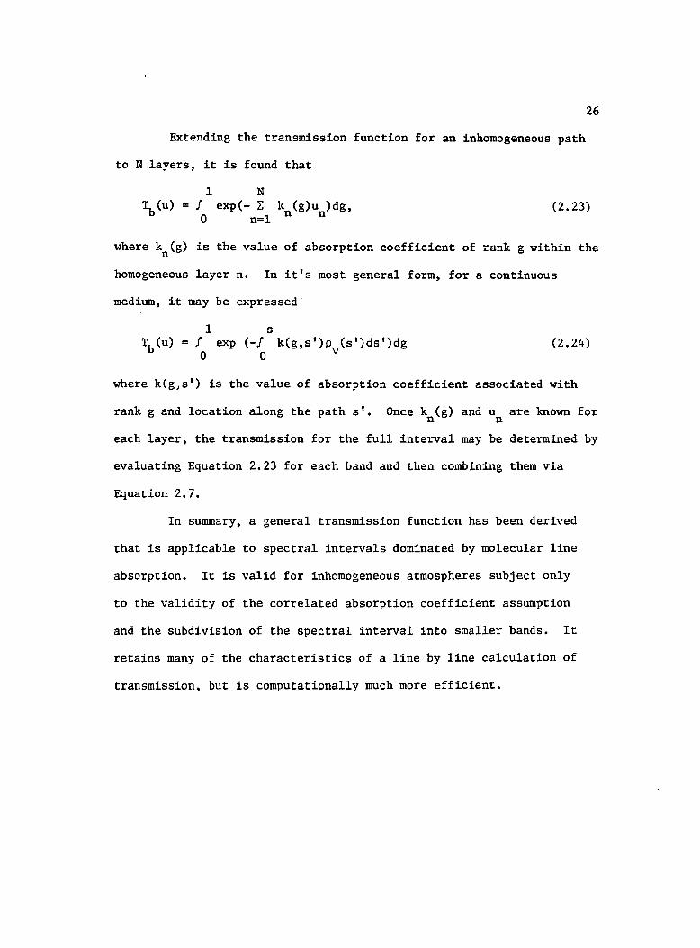
Extending the transmission function for an inhomogeneous path
to N layers, it is found that
1 N Tb(u) = 1 exp(- L It (g)u )dg,
o n=l n n (2.23)
where k (g) is the value of absorption coefficient of rank g within the n
homogeneous layer n. In it's most general form, for a continuous
medium, it may be expressed-
1 s Tb(u) = 1 exp (-I k(g,s')p (s')ds')dg
o 0 \) (2.24)
where k(g)s') is the value of absorption coefficient associated with
rank g and location along the path s'. Once k (g) and u are known for n n
each layer, the transmission for the full interval may be determined by
evaluating Equation 2.23 for each band and then combining them via
Equation 2.7.
In summary, a general transmission function has been derived
that is applicable to spectral intervals dominated by molecular line
absorption. It is valid for inhomogeneous atmospheres subject only
to the validity of the correlated absorption coefficient assumption
and the subdivision of the spectral interval into smaller bands. It
retains many of the characteristics of a line by line calculation of
transmission, but is computationally much more efficient.
CHAPTER 3
THE RADIOMETRIC DETERMINATION OF PRECIPITABLE WATER
An application in which there is considerable interest is the
determination of precipitable water using a ground based radiometer and
in this chapter that problem is addressed. First a general form for
the function k (g) is derived that may be adapted to fit the behavior n
of the absorption bands for normal tropospheric temperatures and pres-
sures. Next, details of the evaluation of the band transmission
integral are discussed as are the sources and natures of the systematic
errors within the model. The effect of random measurement errors on
the precipitable water estimate is discussed and finally a comparison
of the precipitable water determined from the radiometric measurements
and radiosonde measurements is performed.
The Determination of k v
In order to construct k (g), it is necessary to know the n
dependence of the mass absorption coefficient on wave number within the
band. Therefore in this section, the determination of the mass absorp-
tion coefficient at a given wavenumber will be discussed. Also the
dependence of the line parameters, line strength, width, and shape,
on temperature and pressure will be addressed.
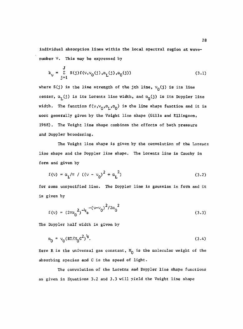
The absorption coefficient at wavenumber v, kv may be expressed
as the summation of the values of absorption coefficient of all the
27
28
individual absorption lines within the local spectral region at wave-
number V. This may be expressed by
J L S(j)f(v,vO(j),aL(j),aO(j»
j=l (3.1)
where S(j) is the line strength of the jth line, VO(j) is its line
center, aL(j) is its Lorentz line width, and aO(j) is its Doppler line
width. The function f(v,vO,aL,aO) is the line shape function and it is
most generally given by the Voight line shape (Gille and Ellingson,
1968). The Voight line shape combines the effects of both pressure
and Doppler broadening.
The Voight line shape is given by the convolution of the Lorentz
line shape and the Doppler line shape. The Lorentz line is Cauchy in
form and given by
(3.2)
for some unspecified line. The Doppler line is gaussian in form and it
is given by
(3.3)
The Doppler half width is given by
(3.4)
Here R is the universal gas constant, MO is the molecular weight of the
absorbing species and C is the speed of light.
The convolution of the Loretnz and Doppler line shape functions
as given in Equations 3.2 and 3.3 will yield the Voight line shape
29
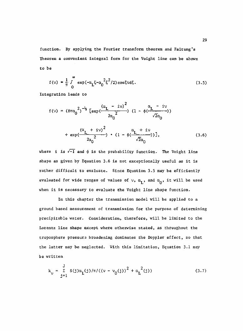
function. By applying the Fourier transform theorem and Faltung's
Theorem a convenient integral form for the Voight line can be shown
to be
00
1 2 2 f(v) = TI ~ exp(-aL~-aO ~ /2)cos~vd~. (3.5)
Integration leads to
f(v) (a
L - iV)2
[exp( 2 ) 2aO
a - iv (1 _ ~( L »
lZaO
(3.6)
where i is r-r and ~ is the probability function. The Voight line
shape as given by Equation 3.6 is not exceptionally useful as it is
rather difficult to evaluate. Since Equation 3.5 may be efficiently
evaluated for wide ranges of values of v, aL
, and aO' it will be used
when it is necessary to evaluate the Voight line shape function.
In this chapter the transmission model will be applied to a
ground based measurement of transmission for the purpose of determining
precipitable water. Consideration, therefore, will be limited to the
Lorentz line shape except where otherwise stated, as throughout the
troposphere pressura broadening dominates the Doppler effect, so that
the latter may be neglected. With this limitation, Equation 3.1 may
be written
k v
J L S(j)aL(j)/TI/«V - VO(j»2 + ~L2(j»
j=l (3.7)
30
where the Lorentz line shape function has been substituted for the
general line shape function.
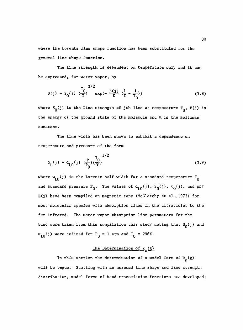
The line strength is dependent on temperature only and it can
be expressed. for water vapor, by
3/2 TO E("n 1 1
(-) exp(-~ (- - -)) T K T TO
(3.8)
where SO(j) is the line strength of jth line at temperature TO' E(j) is
the energy of the ground state of the molecule and K is the Bo1tzman
constant.
The line width has been shown to exhibit a dependence on
temperature and pressure of the form
(3.9)
where aLO(j) is the Lorentz half width for a standard temperature TO
and standard pressure PO' The values of aLO(j), SO(j), VO(j), and paT
E(j) have been compiled on magnetic tape (McClatchy et al., 1973) for
most molecular species with absorption lines in the ultraviolet to the
far infrared. The water vapor absorption line pdrameters for the
band were taken from this compilation this study noting that SO(j) and
aLO(j) were defined for Po = 1 atm and TO = 296K.
The Determination of k ~ n
In this section the determination of a model form of k (g) n
will be begun. Starting with an assumed line shape and line strength
distribution, model forms of band transmission functions are developed;
31
the relationship between the model band transmission functions and
kn(g) will be shown to be dependent only on SO', the equivalent line
strength, and a'L' the equivalent line width. A new technique for the
determination of these parameters will be developed that is based on
the moments of the distribution of mass absorption coefficient within a
specified spectral band and at a given temperature and pressure.
The most intuitive approach to constructing g (k), and therefore n
kn(g), is to randomly select a wavenumber within the band and determine
via Equation 3.7 the value of kv for that wavenumber. By repeating
this a large number of times, it is possible to construct a histogram
of the frequency of occurrence of incremental values of absorption
coefficient. This is the optimal approach in terms of computational
accuracy as with sufficient sampling it is possible to determine g (k) n
to any desired precision. Unfortunately, this technique is extremely
time consuming as a very large sampling of wavenumbers is required to
adequately define g (k) particularly for values of k near zero or n
infinity which are important when the transmission is either low or
high respectively.
Since one of the goals of this research was to develop a
technique that is computationally efficient and the facilities were not
available to execute the sampling approach, use was made of a less
computationally demanding procedure at the cost of surrendering some
degree of accuracy. A model of the distribution of line centers and
line strengths within the band was constructed and from this a model
32
form for g (k) was developed. Then by forcing some characteristics of n
the model g (k) to correctly reproduce some characteristics of the n
true kv' it may be possible to force the model gn(k) to satisfactorily
reproduce the true g (k). The derivation of g (k) will be for a general n n
layer and band and so the nand b subscripts, as shown in Equations 2.7
and 2.23, will be dropped until it is necessary to distinguish between
layers and/or bands.
For the homogeneous path, the band transmission function, as
given by Equation 2.18, can be expressed as the Laplace Transform of
the mass absorption coefficient distribution function, p(k). This is
a convenient behavior because it is very difficult to derive a model
for either p(k) or g(k) directly, but many model forms of transmission
have been developed. Therefore given an analytic model transmission
function, it is possible to determine an analytic form of p(k) via
p(k) = £-1(T(u) ;k) (3.10)
where £-1 (;) is the inverse Laplace transform. The mathematical forms
and properties of Laplace and inverse Laplace Transforms are discussed
in Kreyszig (1979, Chapter 5).
Most of the model band transmission functions are derived by
defining an equivalent line width, W, which represents the width of an
equivalent rectangular line. The rectangular line has the property of
being completely absorbing within the width Wand completely transmit-
ting outside of it. This width has been shown (Goody, 1964), to be
given by
33
00
W = f [1 - exp(Suf(V)]dv (3.11) _00
where f(v) is the line shape function for a band of lines with equal
strength or by
00 00
W = f f [1 - exp(S'uf(v»]p(S')dS'dV -00 0
(3.12)
when there is a distribution of line strengths within the band (Goody,
1964). The value of p(S)dS is the fraction of lines with strengths be-
tween Sand S + dS.
Two forms for p(S) are commonly used in the derivation of trans-
mission functions, the exponential distribution and a Malkmus distribu
-1 -S/So tion in which p(S) is proportional to S e , where So is the mean
line strength. These are chosen since they at least in a broad sense
reproduce the distribution of line strengths observed in most real
absorption bands. Neither reproduces the exact distribution of line
strengths but neither is usually grossly wrong. In Figure 3.1 is given
a comparison of the exponential distribution, the Malkmus distribution,
and the observed distribution for band 7 of SAGE II radiometer water
vapor filter as given in Table 2.1. In this comparison the Malkmus'
distribution agrees well with the observed distribution. For the line
strength distributions of the pcrT band it is usually found that the
Malkmus distribution is in better agreement with the observed distribu-
tion than is the exponential distribution.
At a given wavenumber, the probability that an absorption line
of width W is present is given by W/~v, where ~v is the width of the
1.00
0.75
g(5)
050
o~--~~----~----~--~~--~ 10-3 10-1 100 101 102
5/50
34
Figure 3.1. A comparison of the line strength distributions given by the Malkmus distribution (M), the exponential distribution (E), and the observed line strength distribution (dashed) for band 7 of the SAGE II radiometer's water vapor channel and mean surface conditions
35
band. If there are N lines randomly located within the band, the
probability that n lines are present at any given wavenumber is given
by the Poison probability law in the form
P n
WN -- n
e ~v (WN) / n! ~V
(3.13)
where the expression WN/~V represents the expected number of lines
present at a given wavenumber. Since the transmission function for
these equivalent rectangular absorption lines would be equal to the
fraction of wavenumbers within the band at whi~h no lines are present,
the band transmission function may be expressed as the value of
Equation 3.13 for n = 0 or
T(u) = e -W/o (3.14)
where 0 is the mean spacing between line centers and is defined by
~v/N. (3.15)
The expression W/o is frequently referred to as the equivalent optical
depth of the band.
For an exponential distribution of line strength the equivalent
line width has been shown (Gille and Ellingson, 1968) to have the form
W exp
co
= f (SOuf(v)/l + SOuf(V»)dV -co
(3.16)
where So is the mean line strength. Goody (1952) has shown that for a
Lorentz line shape W has the form exp S u 1/2
W = SOu/(1 + __ 0 __ )
exp TTCLL (3.17)
36
If a distribution of line strengths proportional to S-le-S/SO is
assumed, it can be shown that the equivalent line width has the form
IX)
1 W = - f In(1 + 4 SOuf(v»dV.
M 4-00 (3.18)
For Lorentz line shape, Malkmus (1967) has shown that the equivalent
line width, WM, is given by
~ 7TCX
L 4S
0u
W = - «1 + --) - 1). M 2 7TCX L
(3.19)
An interesting and valuable distinction of the relationship
between T(u) and p(k) is that in many ways, T(u) fulfills the role of
a characteristic function of p(k). Since, according to the model,
p(k) is a unique representation of T(u) via the inverse Laplace trans-
form, either p(k) or T(u) is sufficient to describe completely the
variations of k. Taking successive derivatives with respect to u of
Equation 2.18 and evaluating for an argument of u = 0 we find that
T(n) (u) I = d~~U) I u=O du u=O
or
IX)
f (-k)np(k)dk o
(3.20)
(3.21)
where M is the nth moment. So the moments of the distribution, p(k), n
are characterized by the behavior of the transmission function about
the origin. This is a very convenient relationship as the integral of
Equation 3.20 is usually difficult to evaluate whereas the left hand
side is usually not.
37
From Equations 3.17 and 3.19 it can be seen that the equivalent
line width, W, is a function not only of absorber amount but also of
the parameters So and ~L' The proficiency with which T(u) and therefore
p(k) describes the actual behavior of the band is in large part
dependent on the suitability of values taken for So and ~L' The
standard means of defining these parameters is based upon forcing the
model equivalent optical depth at strong line and weak line absorption
to agree with the true behavior.
The concept of strong or weak line absorption by a gas is based
upon the observed behavior of the transmission for 1imiting1y wide or
narrow line widths. When the absorption lines are narrow, for instance,
both Equations 3.17 and 3.19 may be approximated by the strong line or
square-root approximation for the equivalent optical depth, where w/8
is given by
(3.22)
When the lines are wide, both Equations 3.17 and 3.19 are given by the
so-called weak line or linear approximation, where W/8 is given by
(3.23)
A more general condition for the occurrence of these special cases is
based upon the magnitude of the parameter SOu/TI~L which shall be called
x. When x is much greater than one, W/8 approaches the strong line
approximation, whereas when it is much less than one the equivalent
optiCal depth is approximately given by the weak line form.
38
It has been shown (Godson, 1955a) that for the standard
approach So and a L are given by
S' o (3.24)
and
where the j subscript indicates the jth line within the band. The
equivalent line strength S'O is equal to the mean value of the absorp
tion coefficient in the band. However the equivalent line width, aIL'
is not necessarily the mean line width scaled by the mean line spacing.
These definitions for SIO and aIL serve to force the transmission func
tion to produce the correct transmission as the value of the parameter
x approaches either zero or infinity. Unfortunately, since the band
model of transmission is not a perfect representation of the actual
behavior of a band, it is observed that the value of aIL required to
make the model form of the equivalent optical depth agree with the
observed value is a weak but significant function of the absorber
amount. Godson (1955b) has shown that the error in determining W/8
caused by using aIL as defined by Equation 3.25 can be as large as 5%
in the vicinity of a transmission of 0.50. This behavior is at
least in part due to the fact that aIL has no recollection of the true
line structure, that is, the true placement of lines of differing
strengths relative to one another. This is unfortunate for the applica-
tions considered here as the transmission will nearly always lie
39
between 1.0 and 0.30. It is not feasible to carry the functional
dependence of a'L on u throughout the calculative process, instead it
is preferred to determine a value for a'L which is more indicative of
a mid-range value of transmission.
One way to do this is by invoking the moment generating property
of transmission functions shown in Equation 3.21. From this it can be
shown that the moments of the exponential and the Malkmus transmission
models are functions of S'O and a'L only. For the exponential line
strength distribution, the first three moments of the absorption coef-
ficient distribution can be shown by Equation 3.21 to be
(3.26a)
(3.26b)
and
M = S' 2(1 + 1 ) 2 0 'ITa'
L (3.26c)
The moments of the p(k) for the Malkmus distribution of line strengths
can be shown to be
MO 1.0 (3.27a)
Ml S' 0 (3.27b)
and
M = S' 2(1 +_2_) 2 o 'ITa'
L (3.27c)
The 1th moment can be shown to be given by
, 1 1-1 (1- 1 + k)! -k M = S 0 k:O k! (1 - 1 - k)! (mXo't) 1 (3.28)
for 1 > 1.
40
The moments of kv can also be found directly by averaging the
proper power of kv across the band interval. Thus
J Ml = ~ f kl dv = ~ f [ E k (j)]ldV (3.29)
~v ~v V ~v ~v j=1 V
The evaluation of this equation appears at first to be quite difficult,
but when considering Lorentz line shapes, Equation 3.29 can be solved
for lower orders of moments both efficiently and accurately. The zeroth
order moment is obviously equal to one in agreement with Equation 3.26a
and 3.27a. For 1 = 1, Equation 3.29 may be simplified to
(3.30)
and, for Lorentz line shapes, this is equal to
(3.31)
where wavenumbers vI and V2
represent the upper and lower bounds of the
band. Reasonable simplification reduces Equation 3.31 to
1 J M = - L: S(j).
1 ~v j =1
The second moment, 1 = 2, may be expressed via Equation 3.29 as
1 J 2 J-1 J M2 = ~V [E f k v(j)dV + 2 E E f k (j)k (m)dv]
j=l ~V j=l m=j+l ~v V V
which for Lorentz lines may be approximately expressed as
(3.32)
(3.33)
41
1 J S2~j~ J-1 J 8(j)8(m)
M2 [ L + 2 L L =1v j;l 2rra
L(j)
j=l m=j+1 TI
aL(j) + aL(m)
2J (3.34) vo(m»2 + (aL(j) «vO(j) - + aL(m»
where it is assumed that no line is in the immediate vicinity of the
borders of the band. This assumption has been examined and shown to
have a negligible effect on the determination of the moments and on aIL
The value of 8 1
0 and aIL may now be found by taking the
numerical values for the first and second moments as determined by
Equations 3.32 and 3.34, respectively, and solving via Equations 3.26b
or 3.27b and Equations 3.26c or 3.27c for SIO and aIL' respectively.
In both cases SIO is equal to the first moment but aIL for the exponen
tial model is given by
(3.35)
while in the Malkmus band model aIL is equal to
(3.36)
which results in an equivalent Lorentz half width twice the magnitude
of the former case.
There are some advantages in defining SIO and aIL using the
moments. First of all, since the calculation of the second moment
includes some dependence on the true line structure. the value of a l
L
calculated in this manner has some information on the actual line
structure. Secondly, since Equation 2.18 may be rewritten as
42
T(u) = 1 2 L (-1) mlu II! 1=0
(3.37)
by expanding the exponential into its Taylor series and integrating,
high values of transmission will be determined very accurately. This
occurs because for high transmissions Equation 3.37 may be accurately
approximated as a summation involving only the lowest order moments,
that is
T(u) (3.38)
since u is very small and the summation may be truncated.
Another means of selecting the preferred method to define
S'o and aIL is to select the method which minimizes the effect of the
assumed line strength distribution. Under optimum circumstances the
equivalent line widths predicted by the exponential and Malkmus models
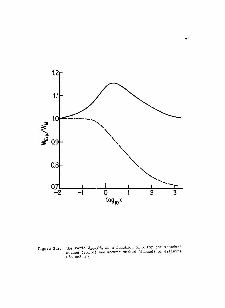
would be identical. However, this is not observed to be the case. In
Figure 3.2 the ratio of equivalent line widths for the exponential
model and the Malkmus model are shown as a function of x which is equal
to S'Ou/TIa'L for both methods of defining S'O and aIL' For the stan
dard method, the ratio approaches 1 for very small and very large
values of x and has a maximum value of 1.16 for x = 2.0. For the
moment method, the ratio is nearly 1 for x < 1 and then approaches
~ as x becomes large. Since x usually is between 0.5 and 20.0 for
the ground based radiometer case, it is apparent that neither method
is superior in this regard. However, for the SAGE II problem, where
1.2
1.1
-----..-. ....... , , , , , , , " " 0.8 " ' ...... ' .......
OJ~----~----~----~----~----'-~~~ -2 -1 0 1 2 3
Figure 3.2.
{og10 x
The ratio Wex /WM as a function of x for the standard method (solid) and moment method (dashed) of defining S'O and a'L
43
44
x is almost always less than 1, the moment method nearly eliminates the
effect of the assumed line strength distribution.
Tables of S'O and a'L are now constructed for each band and
for a range of values of temperature and pressure, by employing Equa-
tion 3.32 and Equations 3.34 and 3.36 respectively. Values of S'O and
a' for a particular band and a particular temperature and pressure may L
accurately be obtained by interpolating across the appropriate table.
The Determination of £-1 [T(u) ;uJ
In this section, the derivation of k(g) will be completed by
evaluating the inverse Laplace transform of the model band transmission
functions. The limiting cases of strong and weak line absorption will
be examined first. The inverse Laplace transforms of the Malkmus and
exponential band transmission functions will be derived in some detail.
In Equation 2.18, it was shown that the relationship between
the mass absorption coefficient distributionfor a homogeneous path is
related to the band transmission function for that path by a Laplace
transform. It therefore follows that if the inverse Laplace transform
may be found for the transmission function that p(k) and ultimately
k(g) may be found.
The complexity of the inverse Laplace transform of the trans-
mission function defined by Equation 3.10 is dependent upon the
functional dependence of the equivalent line width on u. The simplest
inverse occurs for the weak line absorption case where the transmission
function is given by
45
T(u) = exp(-S'Ou) (3.39)
The inverse Laplace transform for this expression may easily be found
to be
p(k) o(k - S'O) (3.40)
where o( ) is the delta function. From the latter expression, it can
be seen that the weak line case is equivalent to a grey body assumption
where the value of absorption coefficient is independent of wavenumber.
The function keg) may be expressed as
keg) = s' o
for all values of g.
(3.41)
The transmission function for the strong line approximation is
given by
(3.42)
and its inverse Laplace transform is found to be
(3.43)
By solving for g(k) using Equation 2.19a and inverting the function it
is found that
-1 keg) = (erf (l
, s' -2 1Tet L 0 g» 4
where erf(x) is the error function which is of the form
2 x erf(x) = - f
/7To
2 -t
e dt.
(3.44)
(3.45)
T(u)
The Malkmus transmission function may be expressed as
1 'ITa' 45' u ~
exp[-~ «1 + 'ITa?) - 1)] L
46
(3.46)
and its inverse Laplace transform may be found using a simple substitu-
tion. In integral form p(k) may be expressed as
Y+';co 'lTct' 1 .... L p(k) = -. f expE---
2n i 2 Y_ co
1 45' u ~
o ] ku «1 +~) - 1 e duo L
(3.47)
Substituting w = u + 'lTct'L/45'0 and dw du it is found that
p(k) (3.48)
This may be written as
p(k) 'lTct\ k -1 1
exp(-4- (2 - 8'».£ (exp(- ('lTS'Oa'tw)~); k) o
(3.49)
then by similarity with the inverse of Equation 3.42, it can be seen
that the mass absorption coefficient distribution is given by
'ITa' S' (k) =! (5' ,)1/2 k-3 / 2 [ __ L (2 - ~ - 2)J
p 2 oct L exp 4 5' k o (3.50)
While no analytic form for k(g) has been found, the function g(k) has
been shown (Domoto, 1974) to be
(3.51)
where erfc( ) is the complementary error function which is usually
available as an intrinsic function on most main frame computers. It
47
is interesting to note that in the limit of strong line absorption
Equation 3.50 approaches the functional form of Equation 3.43 as would
be expected.
The last transmission function to be considered is the exponen-
tial band model which may be expressed
k S' U 2
T(u) = exp[- S'Ou/(1 + TIa~ ) ] L
In integral form p(k) may be expressed as
1
y+ioo S' u ~ p(k) = __ 1 __ f exp[-S'ou/(1 + ~~~ ) ] eku du
2TIi . II~ L y-l.oo
S' u substituting w = ___ 0_ + 1, this may be written as
TIa' L
1 y+ioo TIa'L 1 1 TIa'Lkw [ , ~ -~J [ p(k) = 2TIi f . ~ exp -TIa L (w - w ) exp -s"::':"'-
y-J.oo 0 0
TIa' k - _L-J dw
S' . o
This may be reexpressed by invoking Faltung's theorem, as
1Ta' k L -5-,-)J o
TIa' k L
-S-,-) o
where the * operator indicates a convolution. After some further
manipulation, a final form for p(k) is found to be
(3.52)
(3.53)
(3.54 )
(3.55)
p(k)
co
+ L n=l
('ITa. I ) 3n/2 [ L n! SI n/2
o
'ITa. I S I -~ .!! -1 2(n-1)/2 ( L 0) k2
4
1
48
-'ITa. I S I 'ITa. I S I ~
exp( 8~ 0) D1- n « 2~ 0) )JJ (3.56)
where D (x) is the parabolic cylinder function of the order p. D (x) P P
is defined (Gradshteyn and Ryzhik, 1980, pg. 1064) by the integral
2 -x /4 co -xt-t2/2 -p-l
Dp(x) = erc_p) f e t dt. o
(3.57)
This is not a particularly convenient form for p(k) since at least
twenty terms of the summation are required for reasonable convergence
and values for the parabolic cylinder function are not readily
available.
Figure 3.3 shows a comparison of g(k) for band 2 of the ground
based radiometer for mid tropospheric conditions for the exponential
model, the Malkmus model and the observed absorption coefficient
distribution. It can be seen that for k/S'O greater than about 0.2
both models produced reasonable agreement through the Malkmus model is
somewhat better. For k/S'O less than 0.2 both models tend to under
estimate the value of g probably as a result of over predicting Lhe
presence of very strong lines. While this tendency does not have a
strong effect when k is large, the tails of such lines may contribute
significantly to an over estimation of k when k is fairly small.
1.0
I / ,I
M
// ~
//
,//' //
",~ ". ","'
o· , , , , , 10-3 10-2 10-1 100 10t 102
\/50 Figure 3.3. A comparison of the cumulative absorption coefficient distribution observed in band 2
in the ground based radiometer's water vapor channel for mid-tropospheric conditions (dashed) with that predicted by the exponential model (E) and the Malkmus model (M)
"'" \0
50
At this point, rather than continue consideration of the
exponential model for the mass absorption coefficient distribution
function, attention will be limited to the Ma1kmus model because both
models will yield similar results and the Ma1kmus model is the most
computationally convenient.
The Computation of Transmission
In this section the details of the evaluation of the integral
of Equation 2.23 and the problem of determining precipitable water from
a measured effective optical depth will be addressed. The correlated
absorption coefficient assumption will be evaluated and all other
sources of error in the transmission calculation will be discussed.
A comparison of precipitable water determinations by radiosonde with
those determined radiometrically will also be presented.
The computation of transmission for an individual band for a
given distribution of atmospheric temperature, pressure and water
vapor density is now possible by employing the transmission function
for inhomogeneous paths, as given in Equation 2.23. The value of
k (g) is given by numerically finding the inverse of the mass absorpn
tion coefficient dumu1ative distribution function as given in Equation
3.51 by defining ~'L and S'O using Equations 3.36 and 3.32 respective
ly, for the line parameters of the band in question and the tempera-
ture and pressure of the layer in question.
In executing this integration, a final few simplifying a1tera-
tions have been made. By defining a new variable, h, as the ratio
k/S'O' Equations 2.23 and 3.51 may be changed to
51
1 N f exp[- E h (g) s'o u] dg o n=1 n n n
(3.58)
and
~<l' ~<l' h ~<l' g (h) = 1. [ IT<l'Ln f [ ~ + Ln ] [ Ln n 2 e er c 4h 4 + erfc ~
fITCi'JL -If]] (3.59)
respectively. This has the favorable effect of reducing g (h) to a n
function of <l'L only. Since the integral of either Equation 2.23 or
3.58 must be solved numerically, it is most efficient to tabulate
hn(g) as functions of its independent variables and then interpolate
to the relevant values of hn • By using the transmission function in
the form of Equation 3.58, we may eliminate S'O as a variable in the
above table and thus eliminate the need for one interpolation with a
resulting improvement in accuracy and speed and a reduction in the
volume of computer memory required to store the table. The value of
hn has been tabulated, for the ground based radiometer problem, for 65
values of g between 0.0000 and 1.0000 and for 15 values of a'L between
0.01 and 0.35. The values chosen for <l'L bracket all values charac
teristic of any of the 10 bands for the full range of midlatitude
tropospheric conditions.
The geometry of the ground based radiometer problem is given
in Figure 3.4. The lowest 10km of the atmosphere is divided into ten
lkm thick layers or twenty 0.5km thick layers. A temperature and
pressure for each layer was assigned based upon a surface pressure
- ...... ------
~-R
Range
H
Loyer number -N
_-=:N-1 • • •
• • •
----_____ 3 _____ 2
52
Figure 3.4. The geometry of the ground based radiometer problem where H is a height with an associated horizontal range R for the sun-radiometer line of sight
and temperature and an average lapse rate through the troposphere. A
value for u was determined based upon the above information and upon n
an assumed distribution of atmospheric water vapor mixing ratio (U.S.
53
Standard Atmosphere, 1976). Values for a'Ln and S'On were interpolated
for each band and layer from the previously constructed standard
tables for each. The value of h (g) for each band and layer may be n
determined by interpolating through a' for each of the 65 tabulated Ln
values of g.
The transmission for each band may now be determined by
numerically integrating Equation 3.58, employing an 8th order Romberg
integration. A Romberg integration of the 8th order makes use of 64
intervals in g or 65 points but yields a precision most analogous to
a 256 interval trapezoidal integration; a discussion of the form of
the Romberg integration is given in Stark (1970). For a homogeneous
atmosphere, transmissions calculated via Equation 3.58 should agree
exactly with trans~issions determined via the analytic transmission
function given by Equation 3.46. Comparisons conducted for a wide
range of temperatures, pressures and total precipitable water show
that for the full range of transmissions, from 0.0 to 1.0, the agree-
ment is never worse than 4 significant figures and usually at least
5 digits. For inhomogeneous atmospheres comparisons of the transmis-
sian calculated for the ten layer atmosphere with the twenty layer
atmosphere show agreement to 4 significant figures. On the basis of
these two comparisons it is possible to assert that integration errors
of Equation 3.58 do not significantly contribute to the uncertainty in
54
transmission determination and therefore to the determination of the
precipitable water. A full interval transmission may now be calculated
by combining the transmissions for each band via Equation 2.7.
Discussion
The ultimate goal of this project is not the determination of
the transmission of the paT water vapor absorption band for a given
set of atmospheric conditions but rather the goal is to determine the
precipitable water given a measured water vapor absorption and a
minimum of other a priori information.
The type of a priori information that is required seems to be
limited to knowing the surface temperature and pressure. This effect
can be seen in Figure 3.5 in which the negative of the log of the full
interval transmission, called the effective optical depth, T , is e
plotted against the square root of the vertical precipitable water, u,
times the airmass, m. The airmass is approximately given by the secant
of the solar zenith angle. In this figure there is a curve for
average conditions in Tucson, Arizona (288K, 940mb) and two curves
that yield the most extreme values of transmission for a given amount
of precipitable water for conditions that commonly occur in Tucson.
For a given effective optical depth these curves indicate that there
is a wide range of ±6% in the implied precipitable water depending on
the particular surface conditions. This indicates that for precipita-
ble water determinations at least some accommodation for the ambi~nt
conditions needs to be made.
55
The three curves of Figure 3.5 were determined for an
atmosphere within which the lapse rate is a constant 6.5K/km and the
ratio un /u1 is held constant for all n. These two assumptions do not
have a great effect on the calculated transmissions because, since most
of the water vapor in the atmosphere is located near the ground, the
response to even fairly large variations from the above assumptions is
quite small. This can be seen in Figure 3.6 which shows that about 75%
of the precipitable water under average conditions lies below 3km and
about 75% of the effective optical depth originates below 4km. Trans
mission calculations for lapse rates of 5°K/km and lOoK/km show an
overall difference of 2% in the effective optical depth and therefore
this effect is not of great importance.
The amount of water inferred from a radiometric measurement is
not the vertical precipitable water but it represents a line of sight
vapor amount, being the total amount of water vapor along the path from
the sun to the radiometer. If, as is usually the case, a value for
the vertical precipitable water is desired then it must be assumed
that the atmosphere is horizontally homogeneous for some range about
the radiometer location. The horizontal range, R, is associated with
a height, H, below which a sizeable fraction of the water vapor exists.
A reasonable value for H, from the previous discussion, is about 4km
and since measurements are made for solar zenith angles of 30 degrees
to 80 degrees, this implies the necessary horizontal range is on the
order of 10 to 20km. This is a reasonable assumption and it will not
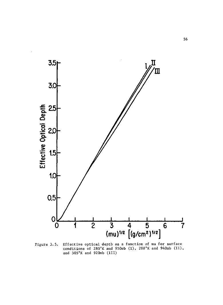
56
3.5
3.0
=2.5 0-Q)
C
c .~ 2.0 ..-0-
0 Q)
.~ 1.5 ..-(.) Q)
'+-'+-lJJ
1.0
2 345 6 (mu )1/2 [(g/cm 2) 112 ]
7
Figure 3.5. Effective optical depth as a function of mu for surface conditions of 280"K and 950mb (I), 288°K and 940mb (II), and 30S o K and 920mb (III)
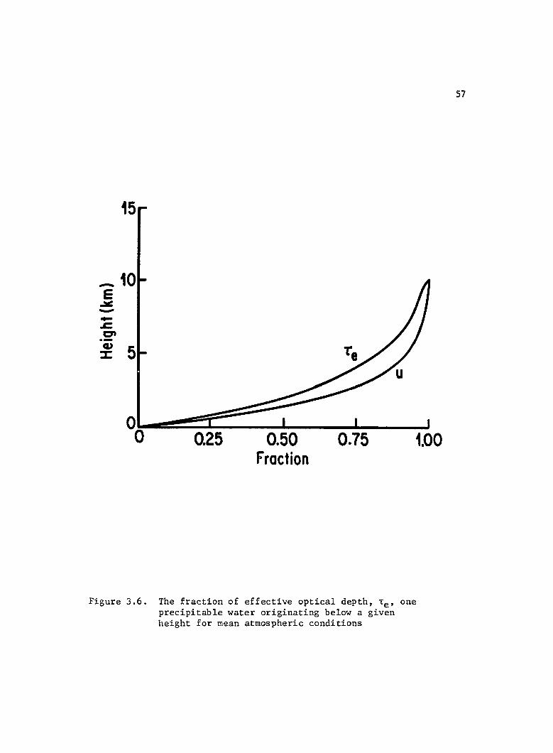
15
- 10 E
...: -~
.c. C' --cu 5 ::J:
~~~~~~ __ -L __ ~ 0.25 0.50 0.75 1.00
Fraction
Figure 3.6. The fraction of effective optical depth, LeI one precipitable water originating below a given height for mean atmospheric conditions
57
58
normally add significantly to the uncertainty in determination of the
local precipitable water.
Given a measured water vapor transmission and the surface
temperature and pressure there are factors which contribute to uncer-
tainties in the implied amount of atmospheric water vapor along the
path. Among the more important of these factors are the specification
of the equivalent Lorentz width a'L' the effect of any failure in the
correlated absorption coefficient assumption, and any random errors
in the water vapor transmission value due to instrument error and/or
to errors in the removal of the effect of attenuation by aerosols and
molecular scatterers.
It is difficult to quantify the effect of the uncertainty in
specifying a' because of the difficulty in separating the error from L
different sources. It is possible, however, to estimate a relative
uncertainty in a'L by defining the parameter in several different but
appropriate ways and comparing the values that are determined. The
variations in the a' ought to be indicative of the overall uncerL
tainty in it.
As an alternative method of defining a'L' it is possible to
determine a value by using the first moment in conjunction with
moments higher than the second. If the true band and the model band
axactly coincided, then the value of a' would be ihdependent of the L
moments used to define it. However, it is observed that a'L is a weak
function of the moments chosen to define it. In Table 3.1 for band 3
of the ground based radiometer, a'L is given as determined via the
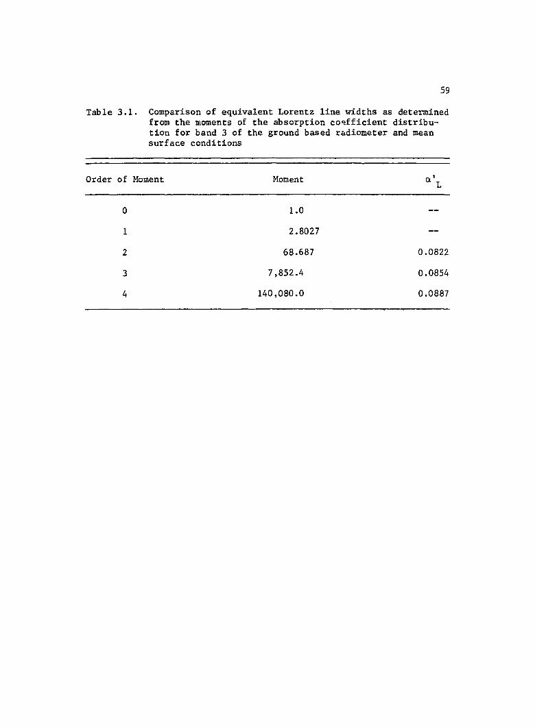
59
Table 3.1. Comparison of equivalent Lorentz line widths as dete1~ined from the moments of the absorption cop.fficient distribution for band 3 of the ground based radiometer and mean surface conditions
Order of Moment Moment Ct' L
° 1.0
1 2.8027
2 68.687 0.0822
3 7,852.4 0.0854
4 140,080.0 0.0887
60
first and second through fourth moments, respectively, and it shows an
overall variation of about 7%. Another method would be to simply use
the standard method of defining a'L as previously described. This
approach yields values of a'L that tend to be somewhat smaller than
the moment defined method being from 20% smaller to 10% larger. This
behavior is indicative of the inability of the model to correctly
predict the full range of possible outcomes with a single value of a'L'
The magnification of an error in a parameter y into an error
in an effective optical depth estimate may be determined by defining
the effective optical depth, Te' to be a function of the parameter to
a power times a constant, or
T = ayP (3.60) e
over a narrow interval in y. For a fractional error in the parameter y
or ~y the rectangular error in Te' ET, is given by
(3.61)
This local power law may be expressed for an infinitesimal interval in
y as
Y dT P=-~
T dy' e
(3.62)
Choosing y to be absorber amount u, the local power law for the band
equivalent optical depth given in Equation 3.19 is given by
-~ ~ p (x) = 2x(l + 4x) 2 «1 + 4x) -1), u
(3.63)
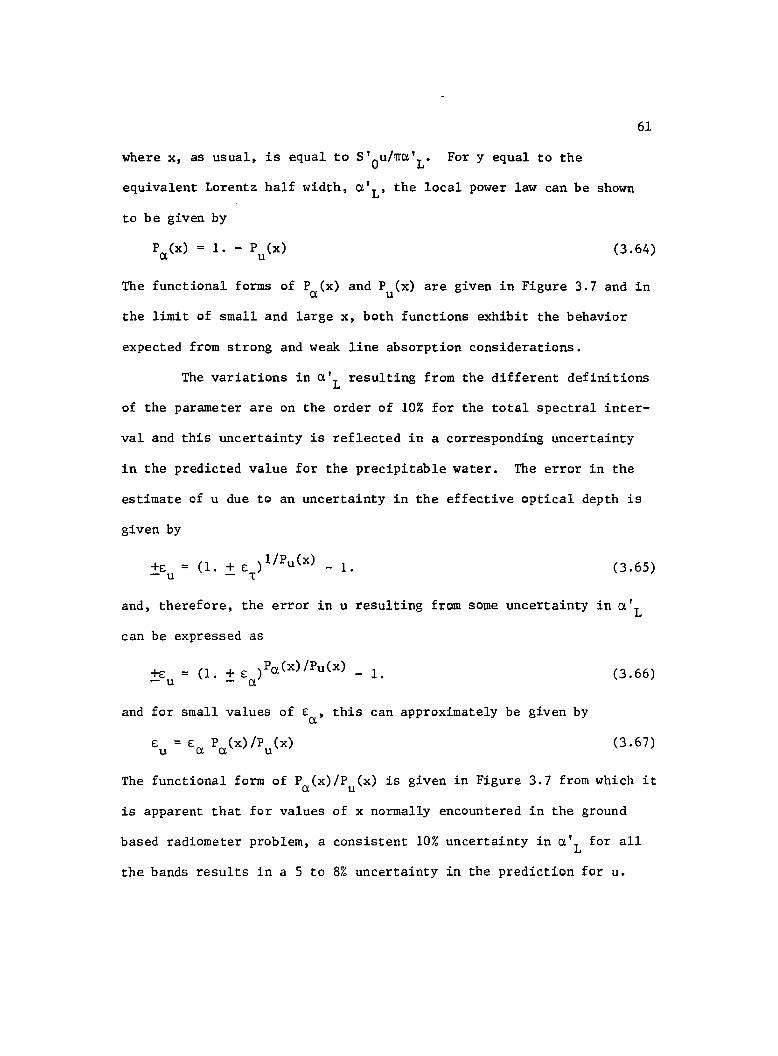
where x, as usual, is equal to S'Ou/~~'L. For y equal to the
equivalent Lorentz half width, ~'L' the local power law can be shown
to be given by
61
P (x) = 1. - P (x) ~ u
(3.64)
The functional forms of P (x) and P (x) are given in Figure 3.7 and in ~ u
the limit of small and large x, both functions exhibit the behavior
expected from strong and weak line absorption considerations.
The variations in a'L resulting from the different definitions
of the parameter are on the order of 10% for the total spectral inter-
val and this uncertainty is reflected in a corresponding uncertainty
in the predicted value for the precipitable water. The error in the
estimate of u due to an uncertainty in the effective optical depth is
given by
(1. + £ )1/Pu (x) - 1. - T
(3.65)
and, therefore, the error in u resulting from some uncertainty in a'L
can be expressed as
and for small values of E • this can approximately be given by a
£ = E P (x) /p (x) u Ct a u
(3.66)
(3.67)
The functional form of P (x)/P (x) is given in Figure 3.7 from which it Ct u
is apparent that for values of x normally encountered in the ground
based radiometer problem, a consistent 10% uncertainty in a'L for all
the bands results in a 5 to 8% uncertainty in the prediction for u.
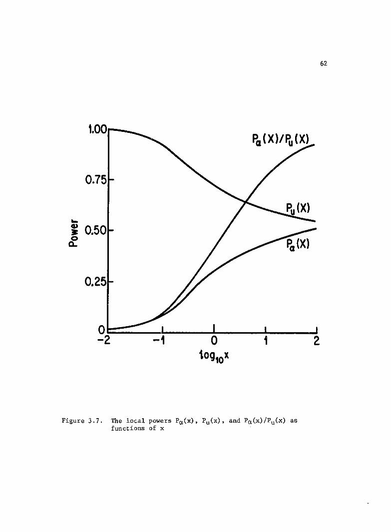
0.75
... ; 0.50 o a..
0.25
o -2-------~1-----0~----1~--~2 tog1ox
Figure 3.7. The local powers PC1 (x) , Pu(x), and PC1 (x)/Pu(x) as functions of x
62
63
This uncertainty is not random in nature but takes the form of biasing
causing the predicted value for u to be consistently either too large
or too small. Note that 8 is defined such that it represents a 95% u
confidence level.
Random errors in the determination of the precipitable water
are a result of random errors in the determination of the water vapor
absorption either due to measurement errors or due to errors in the
removal of the effects of the other attenuators. The effect of these
random errors is given by Equations 3.65 or, for small £ , it may be T
given by
£ = 8 /p (x) u T u
(3.68)
Therefore, random errors in the effective water vapor optical depth
result in a random error in the precipitable water estiIDates whose
magnitudes are from 1.3 to 1.8 times greater for dry and moist cases,
respectively.
The final source of error in the determination of precipitable
water is the effect of the assumption that the rank of the mass absorp-
tion coefficient at a given wavenumber is preserved from one layer in
the atmosphere to any other. Another way of stating this is that the
percentile rank of the absorption coefficient at any wavenumber within
the band is assumed to be independent of temperature and pressure.
The application of this assumption is usually called the correlated
absorption coefficient method.
The correlation coefficient, p, between the mass absorption
coefficient functions, k(v), for two different layers in the
64·
atmosphere or equivalently between the functions at two sets of
temperature and pressure is given by
p (3.69)
where the 1 and 2 subscripts indicate different layers. This equation
may be evaluated relatively easily for both the Lorentz and Voight line
shapes. In Figure 3.8, results showing the correlation between the
k(V) function for certain reference layers with the k(v) function for
layers above the reference layer are exhibited, for a temperature and
pressure distribution as given by the 1976 U.S. Standard Atmosphere.
The value of p decreases rapidly with the distance between the layers
and has dropped below 0.9 for separations of only 6km. It is difficult
to determine from a value of the correlation coefficient a measure of
the uncertainty in determining the correct effective optical depth,
Le' and therefore we will define a new test of the correlation assump
tion. To do this a new function, g(v), is defined such that it repre-
sents the rank of absorption coefficient as a function of wavenumber
for a given temperature and pressure. Then a significant determinator
of appropriateness of the model would be the root mean squared dif-
ference between ~he g(v) functions for different layers. This quantity.
G, is defined by
(3.70)
Under optimal circumstances the value of G would be zero whereas under
the worst circumstances where gl(v) and g2(v) were independent of each
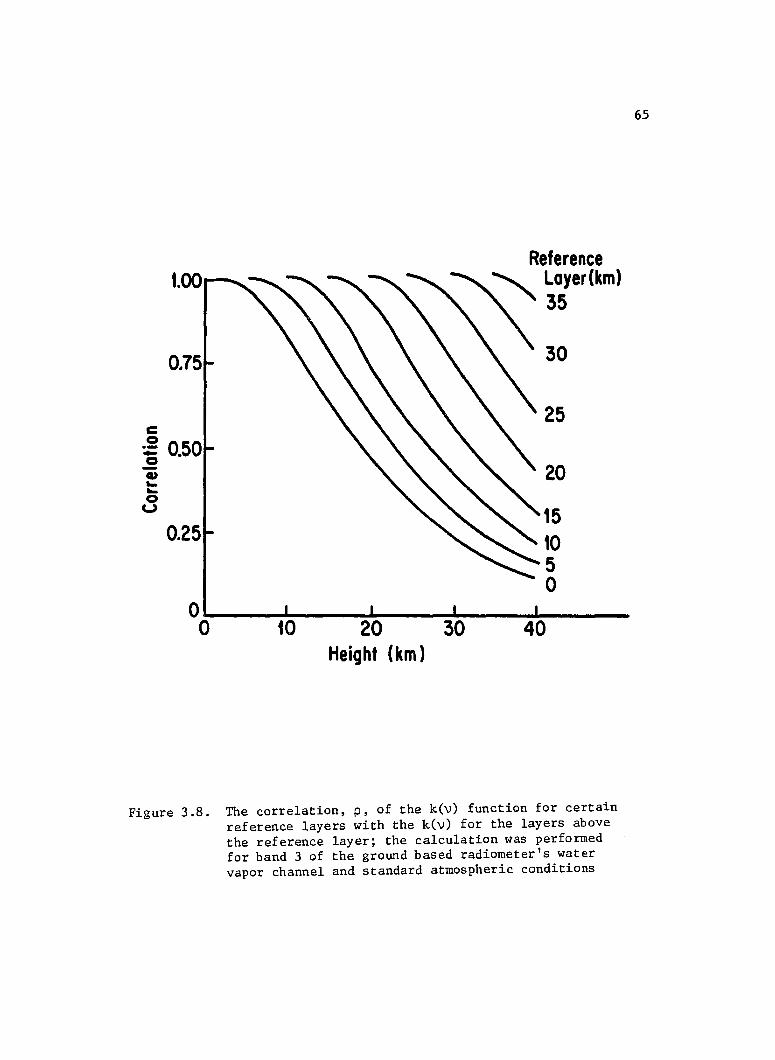
0.75
25 c: .2 0.50 -.E 20 cu ... ... 0 u 15
0.25 10 5 0
0, 0 10 20 30 40
Height (km)
Figure 3.B. The correlation, p, of the k(v) function for certain reference layers with the k(v) for the layers above the reference layer; the calculation was performed for band 3 of the ground based radiometer's water vapor channel and standard atmospheric conditions
65
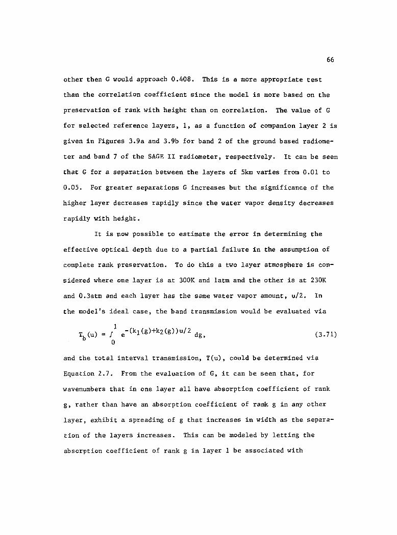
66
other then G would approach 0.408. This is a more appropriate test
than the correlation coefficient since the model is more based on the
preservation of rank with height than on correlation. The value of G
for selected reference layers, 1, as a function of companion layer 2 is
given in Figures 3.9a and 3.9b for band 2 of the ground based radiome-
ter and band 7 of the SAGE II radiometer, respectively. It can be seen
that G for a separation between the layers of Skm varies from 0.01 to
0.05. For greater separations G increases but the significance of the
higher layer decreases rapidly since the water vapor density decreases
rapidly with height.
It is now possible to estimate the error in determining the
effective optical depth due to a partial failure in the assumption of
complete rank preservation. To do this a two layer atmosphere is con-
sidered where one layer is at 300K and latm and the other is at 230K
and 0.3atm and each layer has the same water vapor amount, u/2. In
the model's ideal case, the band transmission would be evaluated via
Tb(u) = J1 e-(k1(g)+k2(g»u/2 dg, o
(3.71)
and the total interval transmission, T(u), could be determined via
Equation 2.7. From the evaluation of G, it can be seen that, for
wavenumbers that in one layer all have absorption coefficient of rank
g, rather than have an absorption coefficient of rank g in any other
layer, exhibit a spreading of g that increases in width as the separa-
tion of the layers increases. This can be modeled by letting the
absorption coefficient of rank g in layer 1 be associated with
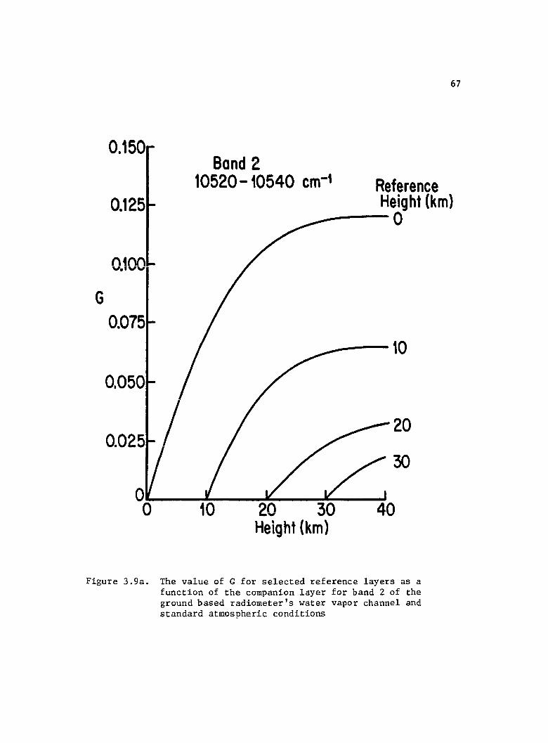
67
0.150 Band 2
0.125 10520 -10540 cm-t Reference
Height (km) ~--O
n1M V.IVV
G 0.075
~--10
0.050
20
30
20 30 40 Height (km)
Figure 3.9a. The value of G for selected reference layers as a function of the companion layer for band 2 of the ground based radiometer's water vapor channel and standard atmospheric conditions
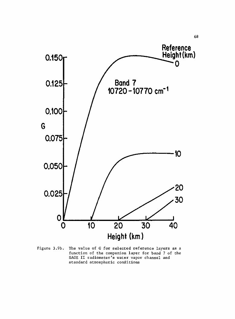
68
0.150 Reference Height (km)
0.125
0.100
G
0.075
0.050
Band 7 10720-10770 cm-1
o
-------10
20 30
o~ ____ ~ ____ ~ __ ~~ __ ~ o 10 20 30 40
Height (km) Figure 3.9b. The value of G for selected reference layers as a
function of the companion layer for band 7 of the SAGE II radiometer's water vapor channel and standard atmospheric conditions
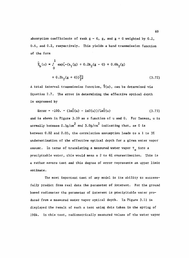
69
absorption coefficients of rank g - G, g, and g + G weighted by 0.2.
0.6, and 0.2, respectively. This yields a band transmission function
of the form
1 J eXP[-(k1(g) + 0.2k2(g - G) + 0.6k2(g) o
(3.72)
A total interval transmission function, T(u), can be determined via
Equation 2.7. The error in determining the effective optical depth
is expressed by
Error = -100 .• (lnT(u) - lnT(u»/lnT(u) (3.73)
and is shown in Figure 3.10 as a function of u and G. For Tucson, u is
normally between 0.5g/cm2 andS.Og/cm2
indicating that, as G is
between 0.02 and 0.05, the correlation assumption leads to a 1 to 3%
underestimation of the effective optical depth for a given water vapor
amount. In terms of translating a measured water vapor T into a e
precipitable water, this would mean a 2 to 6% overestimation. This is
a rather severe test and this degree of error represents an upper limit
estimate.
The most important test of any model is its ability to success-
fully predict from real data the parameter of interest. For the ground
based radiometer the parameter of interest is precipitable water pro-
duced from a measured water vapor optical depth. In Figure 3.11 is
displayed the result of such a test using data taken in the spring of
1984. In this test, radiometrically measured values of the water vapor
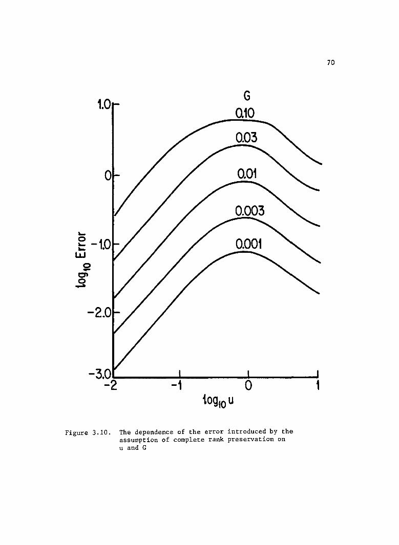
... o ... ... w
o -0'
.3
1.0 G
0.10
0.03
-3.0~ __ ~ ___ --,-___ ....I -2 -1 0 1
Figure 3.10. The dependence of the error introduced by the assumption of complete rank preservation on u and G
70
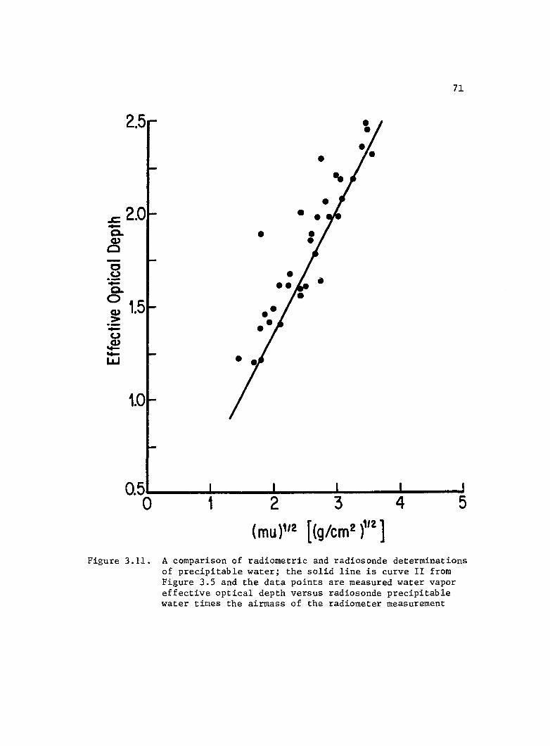
71
Q5~--~----~----~--~----~ o 1 234 5
(mu )1'2 [(g/cm2 )"2 ]
Figure 3.11. A comparison of radiometric and radiosonde determinations of precipitable water; the solid line is curve II from Figure 3.5 and the data points are measured water vapor effective optical depth versus radiosonde precipitable water times the airmass of the radiometer measurement
72
optical depth taken at an air mass of m were plotted against a
precipitable water measurement as inferred from radiosonde measurements
made by the NWS weather station located at Tucson International Airport.
For convenience, the precipitable water was multiplied by the air mass
associated with the radiometric measurement and then taken to the power
of ~ as this made the figure somewhat easier to interpret. It should
also be noted that the radiometer which is located at the University of
Arizona campus and the airport are separated by about 10 miles and the
times of measurements by the radiosonde and the radiometer were
frequently separated by several hours. This leads to some increase in
the scatter of the data points in Figure 3.11 due simply to natural
geographic and temporal variations in the precipitable water.
The transmission model prediction of water vapor effective
optical depth, T , versus total absorber amount, mu, for average Tucson e
conditions, as previously shown in Figure 3.5 is also shown in Figure
3.11. The curve seems to predict the behavior quite well with an RMS
disagreement with data points of 11%. This level of agreement is quite
good since it is the product of errors from not only the model but also
the radiometric determination of the water vapor optical depth and the
radiosonde determination of precipitable water. The radiometric
precipitable water systematically tends to overestimate the radiosonde
precipitable water by about 4%. This biasing may originate in the
model but the value thereof is not particularly worrisome and certainly
does not effect the ability of the model to provide a calibration for
the radiometric measurement of precipitable water.
73
In summary, the complete form of the transmission model has
now been derived for the case of the gro1lnd based radiometric determina
tion of precipitable water. The model can provide inexpensive
calibrations for a wide range of atmospheric conditions that produce
reasonable agreement with radiosonde determinations of precipitable
water. The random difference between the two approaches is a satis
factory 11% with a minimal biasing evident. It is therefore clear that
for the stated purpose of the real time monitoring of precipitable
water, the method developed here is successful in providing the
calibration required by the reduction of the radiometric data.
CHAPTER 4
THE RADIOMETRIC DETEIDfINATION OF
STRATOSPHERIC WATER VAPOR DISTRIBUTIONS
To this point most of the discussion has been limited to the
application of the transmission model to the determination of precipi
table water from measurements made by a ground-based radiometer. In
this chapter the application of the model to the determination of ver
tical water vapor distributions within the stratosphere from single
channel transmission measurements made by a limb scanning satellite
will be considered. There are several significant differences between
the two problems. First, the geometry of the limb scan is much dif
ferent from the geometry of the ground-based radiometer case. The
Voight line shape must be considered rather than just the Lorentz line
shape since in the stratosphere Doppler broadening is significant
relative to pressure broadening. The final difference which must be
addressed is that of retrieving vertical distributions of water vapor
rather than columnar amounts as was previously the case. Thus a
technique must be developed that will allow the reduction of measured
transmission to water vapor density as a functionof height.
In this chapter, these differences will be addressed and a
stratospheric limb scan transmission model will be developed. The
74
reliability of the model is discussed in terms of the effect of the
model assumptions and an inversion process is defined and tested.
Inversion of data taken by SAGE II is performed and compared to re-
suIts obtained from an independent inversion process.
The Stratospheric Limb Scan Transmission Model
A limb scanning satellite such as SAGE II observed the sun
75
through the earth's atmosphere along paths which do not intersect the
surface of the earth. These paths are distinguished from one another
by naming them for the height at which the path comes nearest to the
earth, the tangent height ZT. By rapidly scanning the satellite radio
meter's field of view across the surface of the sun, as it rises or
sets, it is possible to obtain transmission measurements for a wide
range of tangent heights. In Figure 4.1, the geometry of a single
transmission measurement is shown. The most pronounced difference
between this geometry and that of the ground based case as shown in
Figure 3.4 is that while in the ground based case the path length
through each layer was the same, in the limb scan geometry, the path
length is highly dominated by the lowest few layers. The paths would
be similar if ground-based measurements were made for zenith angles
of 900 but they are rarely made for zenith angles greater than 80° •
The geometric distance, Sn(ZT)' that a path with tangent ZT
follows within a given layer is given by
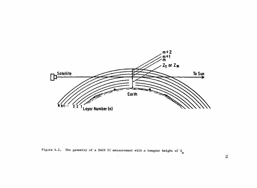
Satellite
m+2 m+t
/"m ZT or Zm
Figure 4.1. The geometry of a SAGE II measurement with a tangent height of Z m
To Sun
-...J 0\
77
(4.1)
where Zn is the height of the top of layer n, RO is the radius of the
earth, ZT is the lowest height the path reaches. This formulation
neglects refraction which must be considered. Refraction in a
spherical atmosphere is a well known process and as such will not be
discussed here; the calculation of Sn(ZT) in a refracting atmosphere is
discussed in Chu (1983).
The band transmission equation given in Equation 2.23 may now
be written as
1 N Tb(u(ZT» = I [exp - r kn(g)q p S (ZT)] dg, o n=m n n n
(4.2)
where q is the water vapor mixing ratio in layer n, N is the total n
number of layers, p is the air density in layer n, and m is the lowest n
layer traversed by the path. The total path water vapor amount,
u(ZT)' is given by
N r q p S (ZT) n n n n=m
(4.3)
The atmospheric layers are defined so that the base of layer m is at
the same altitude as the tangent point as shown in Figure 4.1. There-
fore when reference is made to a specific path with a lowest layer of
m, the tangent height will be called Z. For the SAGE II problem N m
is equal to 37 and the water vapor mixing ratio can be solved for
measurements ~ith tangent heights of 0 to 36km, though usually no
useful data is taken for tangent heights below Skm.
The Determination of k ~ n
78
Equation 4.2 may be evaluated in exactly the same manner as the
band transmission function was solved in the ground based radiometer
case except the function k (g) as previously defined is no longer n
valid. This is because the absorption line shape throughoct the
stratosphere takes on considerable Doppler effects due to the low pres-
sure observed there. The change of line shape can be seen in Figure
4.2 in which the height dependence of the Lorentz, Doppler and Voight
half widths of a single line are shown. The Voight half widths were
calculated using the formula given by Clough et al. (1981). In the
line wings the shape is still essentially Lorentzian but near the
peaks the line shape is significantly different and neglecting this
difference would lead to sizeable errors in the calculation of trans-
mission. Therefore it is necessary to be able to determine a function-
al form for k (g). or at least g (k), that is valid for the n n
temperatures and pressures normally observed in the stratosphere and
the resultant non-Lorentz line shape. The random frequency sampling
technique described in Chapter 3 is the best means to build a valid
assumption-free tabular form of k (g). But, again as described in n
Chapter 3, computational considerations as well as storage considera-
tions prohibit the use of this approach as we are seeking a
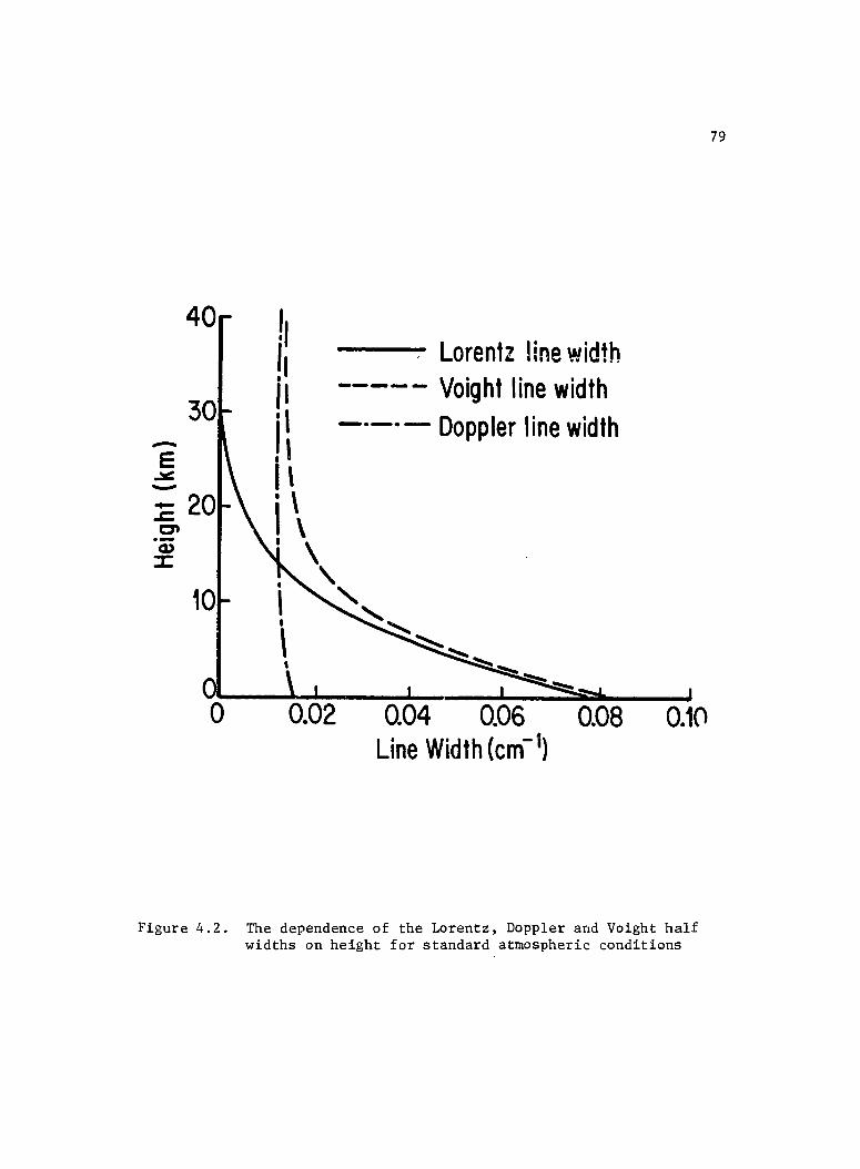
40 ---, Lorentz line width ---- - Voight line width _.-.- Doppler line width -
10
o~ __ ~~ __ ~ __ ~ __ ~~ __ ~ o 0.02 0.04 0.06 0.08 0.10
Line Width (cm-1)
Figure 4.2. The dependence of the Lorentz, Doppler and Voight half widths on height for standard atmospheric conditions
79
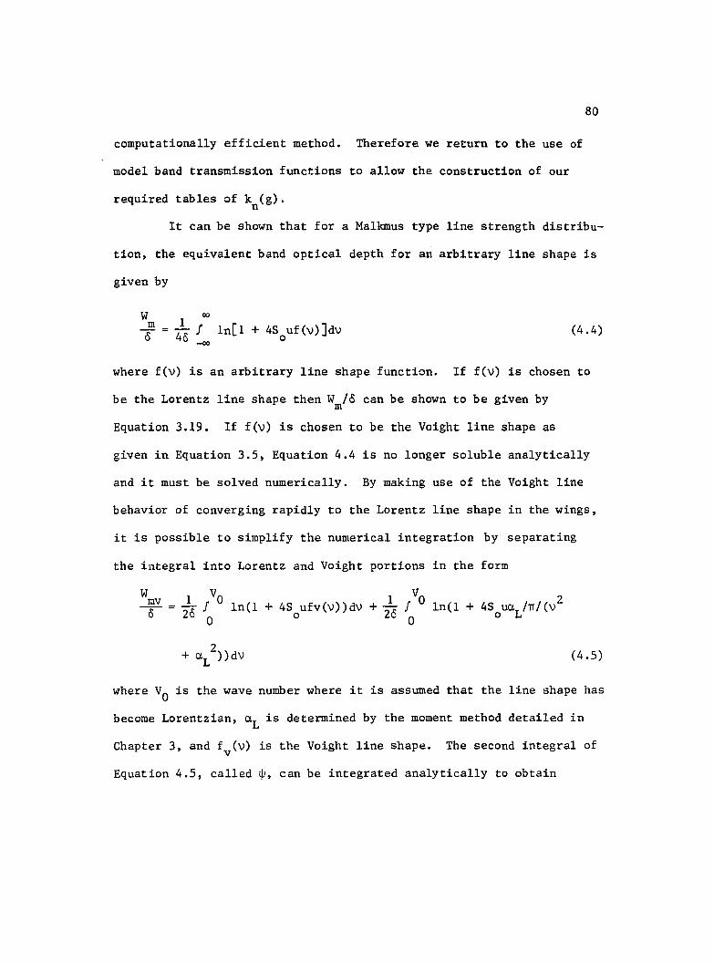
computationally efficient method. Therefore we return to the use of
model band transmission functions to allow the construction of our
required tables of k (g). n
80
It can be shown that for a Malkmus type line strength distribu-
tion, the equivalent band optical depth for an arbitrary line shape is
given by
W co
~ = ~ J 1n[1 + 48 uf(v)]dv (4.4) 8 48 -co 0
where f(v) is an arbitrary line shape function. If f(v) is chosen to
be the Lorentz line shape then W /8 can be shown to be given by m
Equation 3.19. If f(v) is chosen to be the Voight line shape as
given in Equation 3.5, Equation 4.4 is no longer soluble analytically
and it must be solved numerically. By making use of the Voight line
behavior of converging rapidly to the Lorentz line shape in the wings,
it is possible to simplify the numerical integration by separating
the integral into Lorentz and Voight portions in the form
Wmv = __ 1 JVO In(1 + 48 ufv(v»dv + ~ JVa In(1 + 48oU~L/~/(V2 8 28 a 0 20 a
(4.5)
where Vo is the wave number where it is assumed that the line shape has
become Lorentzian, ~L is determined by the moment method detailed in
Chapter 3, and fv(v) is the Voight line shap~. The second integral of
Equation 4.5, called ~, can be integrated analytically to obtain
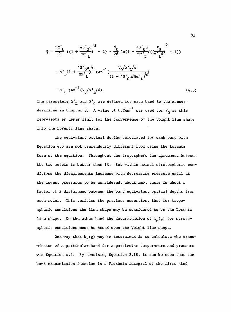
TIet' L
tjJ = -2- «1
1 48' u ~
+ 0) ~
L
81
Vo - 1) - 20 1n(I + 1»
(4.6)
The parameters et'L and S'O are defined for each band in the manner
described in Chapter 3. A value of O.2cm- I was used for Vo as this
represents an upper limit for the convergence of the Voight line shape
into the Lorentz line shape.
The equivalent optical depths calculated for each band with
Equation 4.5 are not tremendously different from using the Lorentz
form of the equation. Throughout the troposphere the agreement between
the two models is better than 1%. But within normal stratospheric con-
ditions the disagreements increase with decreasing pressure until at
the lowest pressures to be considered, about 5mb, there is about a
factor of 2 difference between the band equivalent optical depths from
each model. This verifies the previous assertion, that for tropo-
spheric conditions the line shape may be considered to be the Lorentz
line shape. On the other hand the determination of k (g) for straton
spheric conditions must be based upon the Voight line shape.
One way tha~ k (g) may be determined is to calculate the transn
mission of a particular band for a particular temperature and pressure
via Equation 4.5. By examining Equation 2.18, it can be seen that the
band transmission function is a Fredholm integral of the first kind
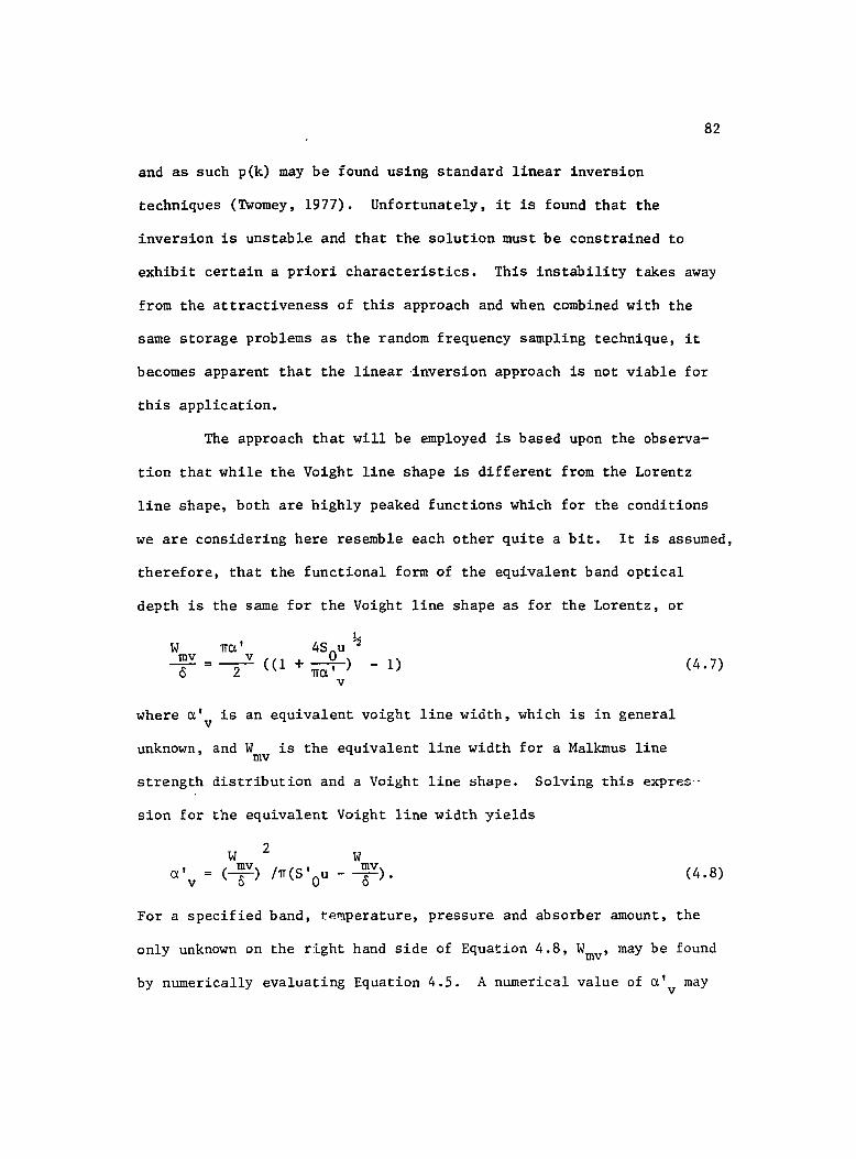
82
and as such p(k) may be found using standard linear inversion
techniques (Twomey, 1977). Unfortunately, it is found that the
inversion is unstable and that the solution must be constrained to
exhibit certain a priori characteristics. This instability takes away
from the attractiveness of this approach and when combined with the
same storage problems as the random frequency sampling technique, it
becomes apparent that the linear ·inversion approach is not viable for
this application.
The approach that will be employed is based upon the observa-
tion that while the Voight line shape is different from the Lorentz
line shape, both are highly peaked functions which for the conditions
we are considering here resemble each other quite a bit. It is assumed,
therefore, that the functional form of the equivalent band optical
depth is the same for the Voight line shape as for the Lorentz, or
W mv -0-
1Ta' v
=-"2 «1 !..:
4S u 2
+ 0) 1Ta'
v - 1)
where a'v is an equivalent voight line width, which is in general
unknown, and W is the equivalent line width for a Malkmus line mv
(4.7)
strength distribution and a Voight line shape. Solving this expres'-
sion for the equivalent Voight line width yields
a' v
(4.8)
For a specified band, tp.~perature, pressure and absorber amount, the
only unknown on the right hand side of Equation 4.8, Wmv ' may be found
by numerically evaluating Equation 4.5. A numerical value of a' may v
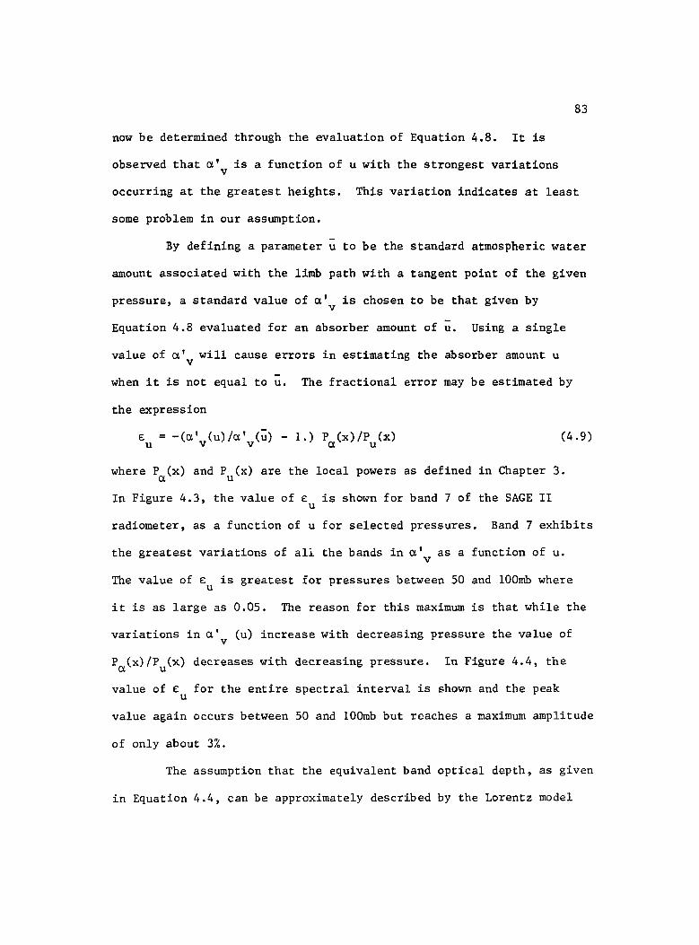
now be determined through the evaluation of Equation 4.8. It is
observed that a' is a function of u with the strongest variations v
83
occurring at the greatest heights. This variation indicates at least
some problem in our assumption.
By defining a parameter u to be the standard atmospheric water
amount associated with the limb path with a tangent point of the given
pressure, a standard value of a' is chosen to be that given by v
Equation 4.8 evaluated for an absorber amount of u. Using a single
value of a' will cause errors in estimating the absorber amount u v
when it is not equal to u. The fractional error may be estimated by
the expression
e: = -(a' (u)/a' (ti) - 1.) p (x)/p (x) u v v a u
(4.9)
where P (x) and P (x) are the local powers as defined in Chapter 3. a u
In Figure 4.3, the value of £ is shown for band 7 of the SAGE II u
radiometer, as a function of u for selected pressures. Band 7 exhibits
the greatest variations of ali the bands in a' as a function of u. v
The value of e: is greatest for pressures between 50 and 100mb where u
it is as large as 0.05. The reason for this maximum is that while the
variations in a' (u) increase with decreasing pressure the value of v
P (x)/P (x) decreases with decreasing pressure. In Figure 4.4. the a u
value of e: for the entire spectral interval is shown and the peak u
value again occurs between 50 and 100mb but reaches a maximum amplitude
of only about 3%.
The assumption that the equivalent band optical depth, as given
in Equation 4.4, can be approximately described by the Lorentz model
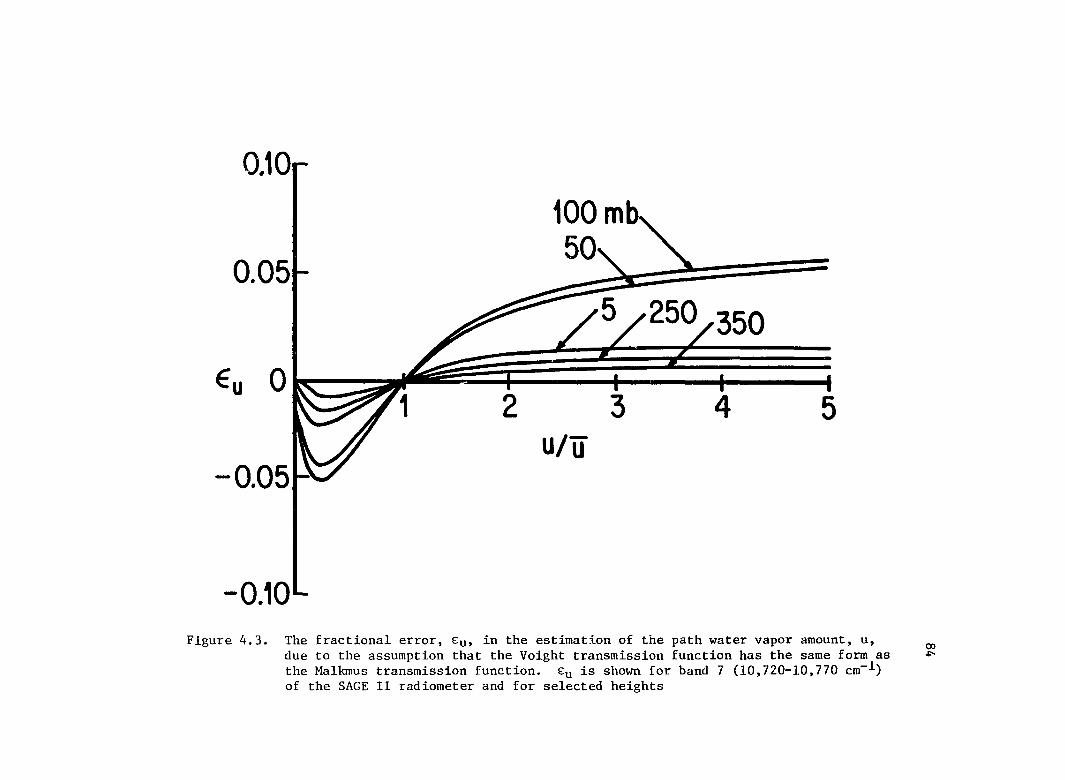
0.10
100mb 50
..... 0.05 ~
Eu c~ 7' r »
I I I - 3 4 5
U/u -0.05"'~
-0.10 Figure 4.3. The fractional error, Eu, in the estimation of the path water vapor amount, u,
due to the assumption that the Voight transmission function has the same form as the Ma1kmus transmission function. Eu is shown for band 7 (10,720-10,770 cm-1) of the SAGE II radiometer and for selected heights
00 ~
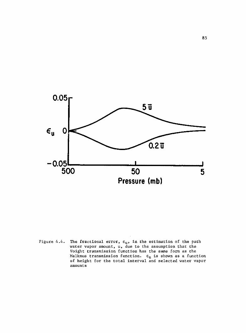
85
0.05
-0.05--------,a.,....---_--' 500 50
Pressure (mb) 5
Figure 4.4. The fractional error, Eu' in the estimation of the path water vapor amount, u, due to the assumption that the Voight transmission function has the same form as the Malkmus transmission function. Eu is shown as a function of height for the total interval and selected water vapor amounts
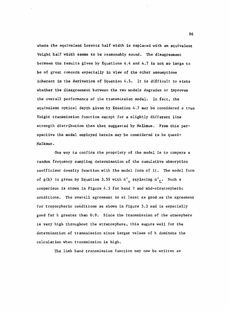
86
where the equivalent Lorentz half width is replaced with an equivalent
Voight half width seems to be reasonably sound. The disagreement
between the results given by Equations 4.4 and 4.7 is not so large to
be of great concern especially in view of the other assumptions
inherent in the derivation of Equation 4.5. It is difficult to state
whether the disagreement between the two models degrades or improves
the overall performance of the transmission model. In fact, the
equivalent optical depth given by Equation 4.7 may be considered a true
Voight transmission function except for a slightly different line
strength distribution than that suggested by Malkmus. From this per-
spective the model employed herein may be considered to be quasi-
Malkmus.
One way to confirm the propriety of the model is to compare a
random frequency sampling determination of the cumulative absorption
coefficient density function with the model form of it. The model form
of g(h) is given by Equation 3.59 with a l replacing aIL. Such a v
comparison is shown in Figure 4.5 for band 7 and mid-stratospheric
conditions. The overall agreement is at least as good as the agreement
for tropospheric conditions as shown in Figure 3.3 and is especially
good for h greater than 0.9. Since the transmission of the atmosphere
is very high throughout the stratosphere, this augurs well for the
determination of transmission since larger values of h dominate the
calculation when transmission is high.
The limb band transmission function may now be written as
10-2 10-1 h
tOO tot
Figure 4.5. The model g(h) (dashed) and the true g(h) (solid) for band 7 of the SAGE II radiometer and mid-stratospheric conditions
102
co .......
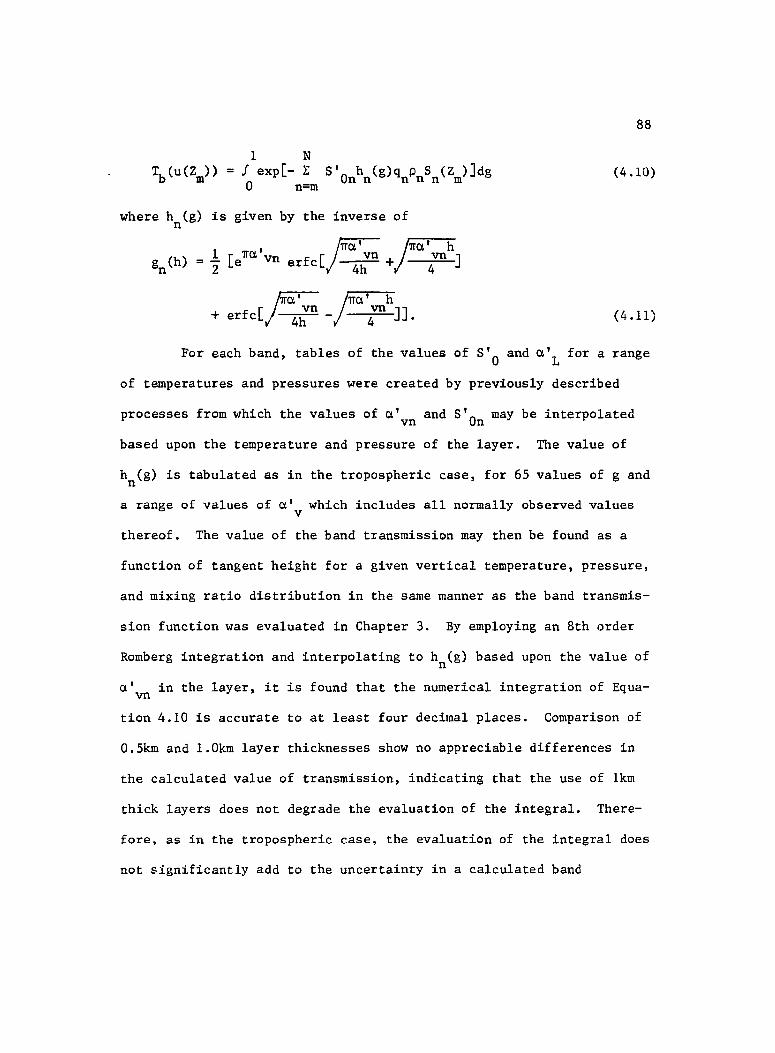
88
1 N = ! exp[- I: S'o h (g)q P 8 (Z )Jdg nn nnn m (4.10)
a n=m
where h (g) is given by the inverse of n
~~ gn(h) = 1 [e
7Ta.'vn erfc[/T +/--f!LJ
~~ + erfc[/T -/--f!LJJ. (4.11)
For each band, tables of the values of 8'0 and a.'L for a range
of temperatures and pressures were created by previously described
processes from which the values of a.'vn and S'On may be interpolated
based upon the temperature and pressure of the layer. The value of
h (g) is tabulated as in the tropospheric case, for 65 values of g and n
a range of values of a.' which includes all normally observed values v
thereof. The value of the band transmission may then be found as a
function of tangent height for a given vertical temperature, pressure,
and mixing ratio distribution in the same manner as the band transmis-
sion function was evaluated in Chapter 3. By employing an 8th order
Romberg integration and interpolating to h (g) based upon the value of n
a.' in the layer, it is found that the numerical integration of Equavn
tion 4.10 is accurate to at least four decimal places. Comparison of
0.5km and 1.Okm layer thicknesses show no appreciable differences in
the calculated value of transmission, indicating that the use of 1km
thick layers does not degrade the evaluation of the integral. There-
fore, as in the tropospheric case, the evaluation of the integral does
not significantly add to the uncertainty in a calculated band
89
transmission for any given set of atmospheric conditions. The
transmission for the entire interval may be calculated by evaluating
Equation 4.10 for each band and then combining them via Equation 2.7.
The Determination of the Vertical Water Vapor Distribution
The goal of this project is not to determine transmittance for
limb paths through the stratosphere but to use measured water vapor
transmittances to infer vertical water vapor distributions. Since the
relationship between transmission and the vertical water vapor
distribution is not linear, the determination of q(z) or rather qn for
all n cannot be directly performed. In this section an iterative
reduction technique will be developed that is both numerically stable
and rapidly conveTgent.
The derivation of the reduction technique is started by recall-
ing from Chapter 3 that it is possible to define a local power law
relating the dependence of two parameters by the expression
p - ~ Ex. x - Y dx (4.12)
p where y = ax x over some interval in x. If y is defined as the effec-
tive water vapor optical depth, that is the negative of the natural
logarithm of the transmission for the total interval, Te = -In(T(u)),
and x is the absorber amount, then it is possible to determine a local
power law for any limb path. This may be expressed as
(4.13)
90
Pu(ZT) is dependent not only on u and ZT but also on the temperature
and pressure at and above the tangent point. Rather than determining
Pu(ZT) as a function of temperature and pressure, a standard set of
Pu(ZT) curves is determined for standard atmospheric conditions. This
is done by first determining a set of curves of Te(ZT) versus u(ZT)
for standard atmospheric conditions (U.S. Standard Atmosphere, 1976)
via Equations 4.10 and 2.7. The value of u(ZT) was varied in order to
include all possible conditions by multiplying the standard distribu-
tion of water vapor mixing ratio by a constant whose value was between
10-3 and 10+3 • The standard curves of Te(ZT) are shown in Figure 4.6.
Standard curves of Pu(ZT) are found from the information contained in
Figure 4.6 and are themselves shown in Figure 4.7.
For the reduction technique, the information of Figure 4.6 was
tabulated such that u(ZT) was given as a function of the effective
optical depth and the tangent height. Figure 4.7 was tabulated such
that Pu(ZT) was given as a function of u(ZT) and tangent height.
Given a measured value of effective optical depth for a limb path m
with tangent height Z , it is now possible to estimate the value of m
u(Z ) by interpolating across the tabulated form of Figure 4.6 with m
respect to effective optical depth and tangent height. For instance,
if Z is 20km and T (20km) was determined to be 0.1, indicating a m e
total interval transmission of 0.905, u(20km) can be estimated to be
2 0.36g/cm. Therefore for a set of effective optical depth measure-
ments, it is possible to estimate a corresponding set of path water
vapor amounts. Note that the measurements are made such that they have
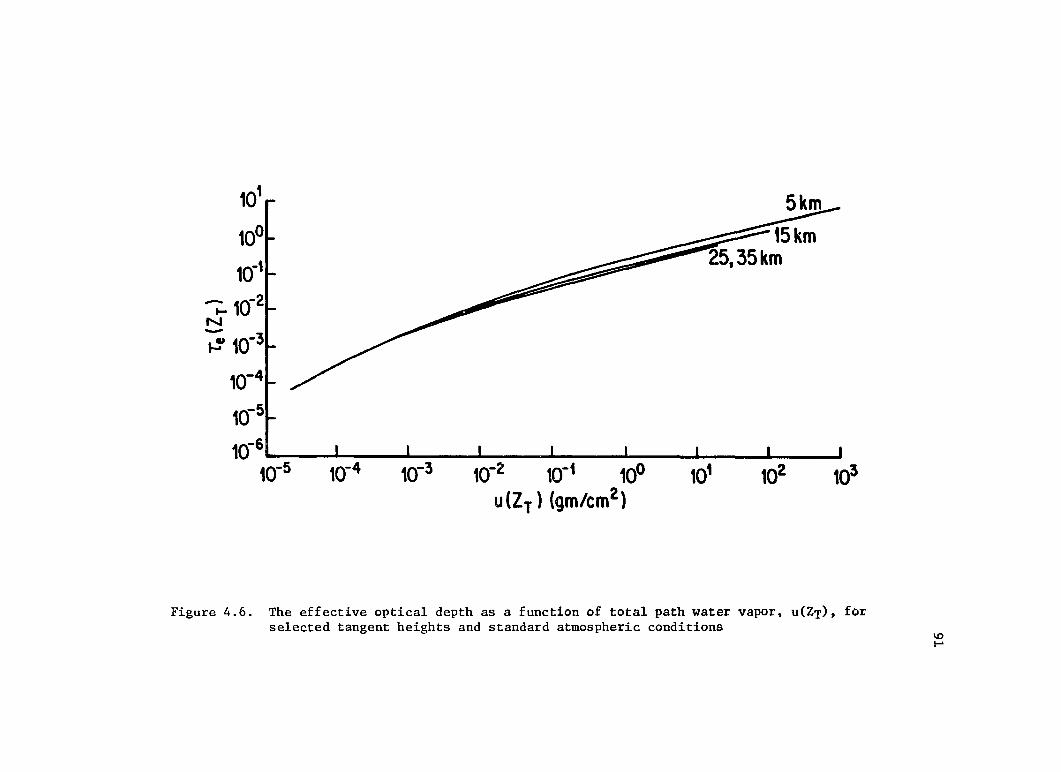
10'
10°
10-1
-;"10-2 N
~ 10-3
10-4
10-5
5km ...-
~15km 25,35km
10-6. , , , , , , , ,
10-5 10-4 10-3 10-2 10-t 10° 10' 102 103
U (ZT) (gm/cm2)
Figure 4.6. The effective optical depth as a function of total path water vapor, U(ZT), for selected tangent heights and standard atmospheric conditions
\0 I-'
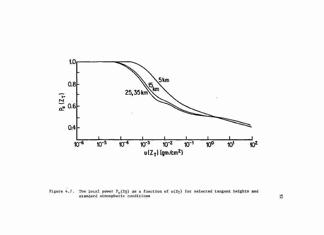
1.0. zc:: --
10-6 10-3 10-2 10-1 102
u(ly) (gm/cm2)
Figure 4.7. The local power Pu(ZT) as a function of U(ZT) for selected tangent heights and standard atmospheric conditions \0
N
93
tangent heights spaced 1km apart and are defined such that they end
at the base of the last layer in the transmission calculation, usually
36km.
The relationship between u(Z ) and the water vapor mixing ratio m
distribution with height is given by Equation 4.3. With the set of
u(Z ) estimates it is possible to record this relationship in matrix m
form as
u Dq (4.14)
where um is u(Zm) , qn is the mixing ratio in layer nand Dmn is given
by
D mn
p s (Z ) n n m
for n > m and by
D mn o.
when n < m. The true pressure and temperature distributions with
(4.15)
(4.16)
height are presumed to be known and the air density p and path length, n
s (Z ), within layer n for a limb path of tangent height Z are com-n m m
puted for the true atmospheric conditions. The so-called onion skin
solution for q is then given by
-1 q = D u (4.17)
and a least squares solution for 2 is given by
where the T superscript indicates a matrix transpose. Solutions for q
from the two above approaches are nearly identical because the
94
determination of q is highly dominated by the value of u. The n n
reduction employed here usee the least squares solution for ~.
The vectors ~ and ~ represent the first guess solutions for
1 1 the water vapor distribution and are designated as such by u and q - -Since ~1 is based upon a model atmosphere whose temperature and pres
sure distributions may be in significant variance with the true atmos-
1 1 phere, the values of ~~ and ~ may be significantly in error. A first
guess estimate of the effective optical depth for tangent height Z m
may be determined by employing Equations 4.10 and 2.7 where Pn
,
S (Z ), S'O and a' are determined in accordance with the true n m n vn
atmospheric conditions and q is chosen to be equal to q 1; this n n
estimate is designated by L 1(Z). Comparisons of L 1(Z ) with the e m e m
measured value, L (Z ), typically show disagreements of 0 to 50%; the e m
size of which is indicative of the validity of the first guess values
of q and u. Ideally the itera~ive technique to be described will
reduce these differences to essentially zero.
A second guess of u(Z ) may be determined by applying the m
local power law assumption previously used to estimate error magnifi-
cation. From Equation 4 .13, it can be seen that over a narrO\\1 range
of u that
L (Z ) e m
where a is a constant. The second guess value of u(Z ), m
(4.19)
is now
determined by assuming the difference between the measured effective
optical depth, T (Z ), and the estimated value, T l(Z ), is due e m e m
strictly to an error in the first guess value of path water vapor
1 u (Z ).
m The value of u2 (Z ) is given, therefore, by
m
95
(4.20)
and the second guess value of ~ may be found by Equation 4.18 where
2 u = u. The value of P (Z ) is determined from the tabulated form of u m
Figure 4.7 interpolated for the appropriate values of tangent height
and absorber amount. -2 For the previous example of u(20km) = 0.36g/cm
the value of P (20km) is found to be 0.56. u
A new estimated value of the effective optical depth, T 2(Z ), e m
is then determined again using Equations 4.10 and 2.7 and is found to
be in better overall agreement with the measured value than was the
first guess, T 1(Z). By repeating this power law iteration a suffie m
cient number of times very nearly any degree of numerical agreement
between the measured set of T (Z ) and the estimated set of effective e m
water vapor optical depths is possible. The general form of the jth
estimate for the path water vapor amount is given by
) (Z ) m
·1 ·1 1/Pu (Zm) uJ - (Z ) (T (Z )/T J- (Z »
m e m e m (4.21)
where the ratio T (Z )/T j-1(Z ) approaches 1 as j increases. e m e m
It is in general found that two iterations are sufficient to
bring the mean disagreement between the estimated and the measured
effective water vapor optical depths to less than 0.5% and three
iterations bring the mean disagreement to less than 0.2%. In Figure
123 4.8, a comparison of ~ , ~ , and ~ is shown for a set of SAGE II
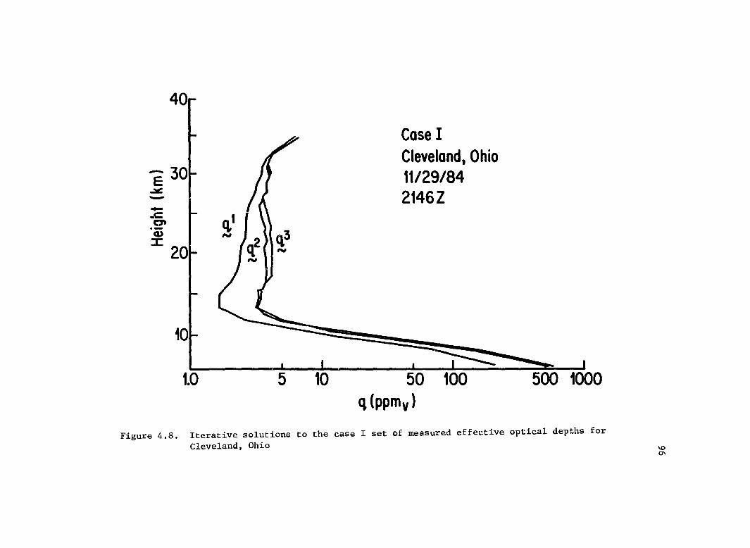
--..c: C' Q)
::J:
10
1.0
q,' -
Case I Cleveland, Ohio 11/29/84 2146Z
50 q (ppmv)
500 1000
Figure 4.8. Iterative solutions to the case I set of measured effective optical depths for Cleveland, Ohio \0
0\
97
measurements taken over Cleveland, Ohio on 11/29/84 at 2146Z and it can
be seen that there is a rapid convergence to a steady solution. The
solution ~4 is not plotted on Figure 4.8 simply because it could not
be distinguished f"-om ~3.
One of the favorable aspects of the iterative technique is the
fact that neither the first guess values for path water vapor amount,
1 u , or the values of P (Z ) pl;y a decisive role in the final solution u m
determined for the water vapor mixing ratio distribution. It ndght be
1 expected that since both u and P (Z ) were determined for particular u m
atmospheric conditions that some biasing in the final solution might
result if the true atmospheric conditions were significantly different.
But the solution toward which the iterative solutions converge is
unique and the process by which the progressive estimates for q are
determined only serves to govern the rapidity with which that solution
is approached. The reason that the power law iteration was used is
not because it adds any information to the reduction process but be-
cause it very rapidly converges toward the unique solution. In fact
even under extreme atmospheric conditions, the progressive mixing ratio
estimates rapidly converge.
Discussion
A method for the determination of the vertical water vapor
distribution has now been developed. Given a set of limb transmit-
tances as a function of path tangent height. there are factors which
contribute to the uncertainty in the determined water vapor profiles.
98
Among the more important of these factors are horizontal homogeneity,
random measurement errors, errors in the assumed atmospheric tempera-
ture distribution, the specification of~' , and the effect of any v
failure in the correlated absorption coefficient assumption.
By examining Equation 4.10 it can be seen that there is an
implicit assumption that the atmosphere is horizontally homogeneous
since S'O ,a' and q are considered to be independent of the hori-n vn n
zontal locat~on within the layer. Since the water vapor density
decreases rapidly with height, an assumption that the atmosphere is
horizontally homogeneous is not significant for the full depth of the
atmosphere. It is instead found for a particular paths that a large
fraction of the attenuation occurs within a relatively small vertical
distance of the tangent height and horizontal homogeneity need be
maintained only below this height. The fraction of optical depth
originating below some height may be defined by
(4.22)
where Tl (u(Zm)) is given by
1 N f exp[- L S'O h (g)p S (Z )]dg. o n=m+l n n n n m
(4.23)
The value of gT(l) for standard atmospheric conditions and tangent
height paths of 5, 15 and 2skm is given in Figure 4.9. On average it
is found that about 75% of the attenuation originates within skm of
the tangent height. This is very nearly the same thickness as was
required for the ground based radiometer but due to path geometric
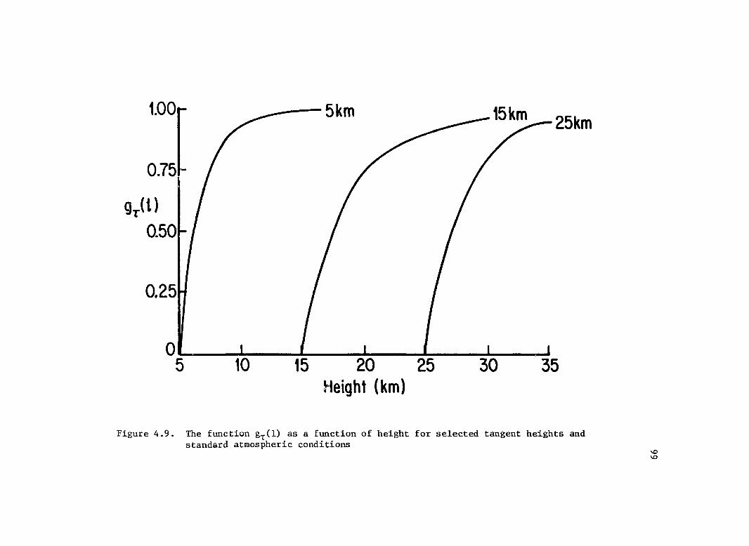
1.00 --5km 15km 25km
0.75--
0.25
o· , , , , , , 5 10 15 20 25 30 35
Height (km)
Figure 4.9. The function gT(l) as a function of height for selected tangent heights and standard atmospheric conditions
1.0 1.0
100
differences, a 5km height now implies a horizontal homogeneity
requirement of about 500km. Below the tropopause assuming that the
atmosphere is horizontally homogeneous on the scale of 500km is
frequently not valid and it will often lead to a degradation of solu'-
tion. Within the stratosphere, this range presents less of a problem
as the stratosphere is more homogeneous than the troposphere
(Ellsaesser, 1983). However, it still represents a significant diffi-
culty in the interpretation of an estimated vertical water vapor
distribution. Horizontal inhomogeneities within a particular layer
cause the estimates of water vapor mixing ratios in layers within
3 to 4km of that layer to be in error.
The magnification of random errors in the effective optical
depth to errors in the path water vapor has been discussed, and this
error is not passed on unaffected to the vertical water vapor distribu-
tion estimate. It has been shown (Frieden, 1983) that for a least
squares solution for q as given in Equation 4.18, a covariance matrix,
c, may be expressed as
c (4.24)
2 where cr is the variance of the uncertainty in the elements of the
u
vector u. The fractional uncertainty in the solution element q is n
given by
k 2C;! /q
nn n (4.25)
and the normalized correlation between solution element qn and qm is
given by
101
p(m,n) = C I(c c )~ mn mm nn (4.26)
The covariance matrix was derived for additive noise of zero mean and
for the case that the solution vector, q, is an unbiased estimator of
the true solution. If cr 2 is not constant for each element of the path u
water vapor vector, u, then the covariance matrix is given by
c (4.27)
2 where V is a diagonal matrix with elements of cr or the variance of un
the noise in each element of the path water vapor vector. In Figure
4.10 is shown a plot of E for standard atmospheric conditions and a q
realistic value of a which is 10% of the limb path water vapor amount un
u. The most important inference that can be made from this figure is n
that errors in the path water vapor amount are magnified by about a
factor of 2.5 in mixing ratio estimates.
The correlation between the various layers seems to be fairly
stationary through the full atmosphere. If Equation 4.26 is rewritten
as
p(n,n+~n) = p(n,m) (4.28)
then it is found that the correlation is nearly independent of nand
mainly dependent on the separation ~n. In Table 4.1 is shown the mean
behavior of the correlation as a function of ~n. The value of p is
negative and decreases rapidly as \6n\ becomes large. The vertical
resolution that this implies is on the order of 1 to 2km depending
upon the size of the feature to be resolved.
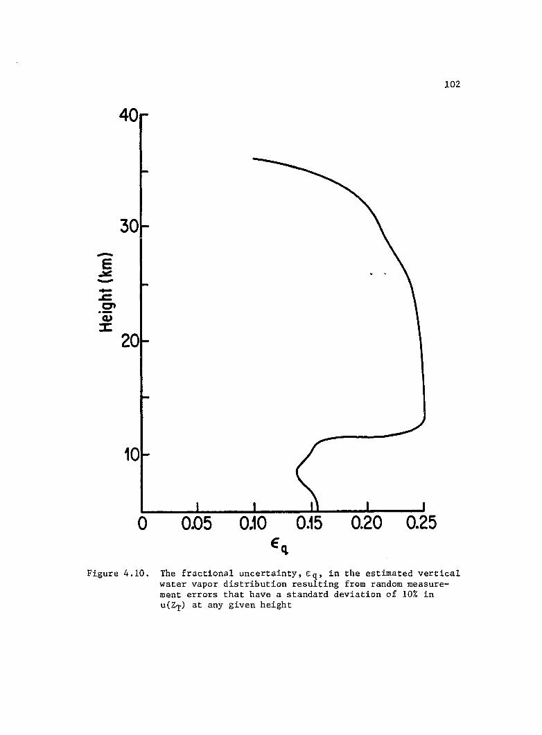
102
40
30
-E -'ttl! -.... .c .2' Q)
~
20
10
o 0.05 0.10 0.15 0.20 0.25
Figure 4.10. The fractional uncertainty, Eq, in the estimated vertical water vapor distribution resulting from random measurement errors that have a standard deviation of 10% in u(ZT) at any given height
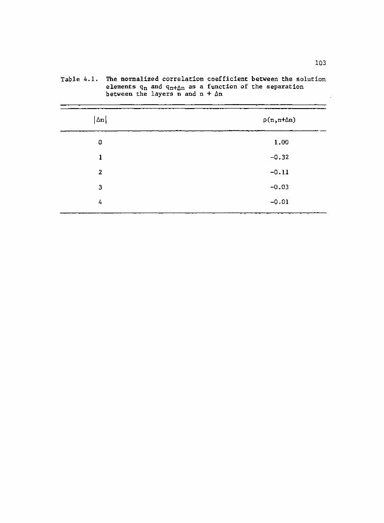
103
Table 4.1. The normalized correlation coefficient between the solution elements qn and qn+~n as a function of the separation between the layers nand n + ~n
I~nl p(n,n+~n)
0 1.00
1 -0.32
2 -0.11
3 -0.03
4 -0.01
104
The reduction of limb transmission data to water vapor mixing
ratio profiles is based upon the assumption that the thermal structure
of the atmosphere is known. Since the temperature profile is usually
determined by remote sensing techniques, there is a resulting uncer-
tainty in the inferred temperature profile and ultimately in the
inferred water vapor distribution. In Figure 4.11 is shown the error
in the estimated water vapor mixing ratio at a particular height given
a locally systematic error in the vertical temperature profile of ~T.
A typical 95% confidence limit in a remotely determined temperature
profile is about +5°K and that corresponds to an uncertainty in q of n
about ±4%. The magnitude of this uncertainty is relatively independent
of height varying over the full atmosphere from ±3% to ±5%.
The specification of~' is a source of biasing in the v
inference of vertical water vapor distributions just as in the ground
based radiometer problem where the specification of ~'L was a source
of biasing. The problem in this case, is in fact the problem in
specifying ~'L which is incorporated into the determination of ~'v'
As in the ground based problem, the uncertainty in ~'L is about 10%
but the importance of it in the determination of ~'v decreases with
increasing altitude so that uncertainty in ~'L has progressively less
effect on the uncertainty in the water vapor mixing ratio. In Figure
4.12 the fractional uncertainty in the water vapor mixing ratio Eq ,
due to the uncertainty in a' as a function of height is shown for v
standard atmospheric conditions.
confidence limit.
The value of E represents a 95% q
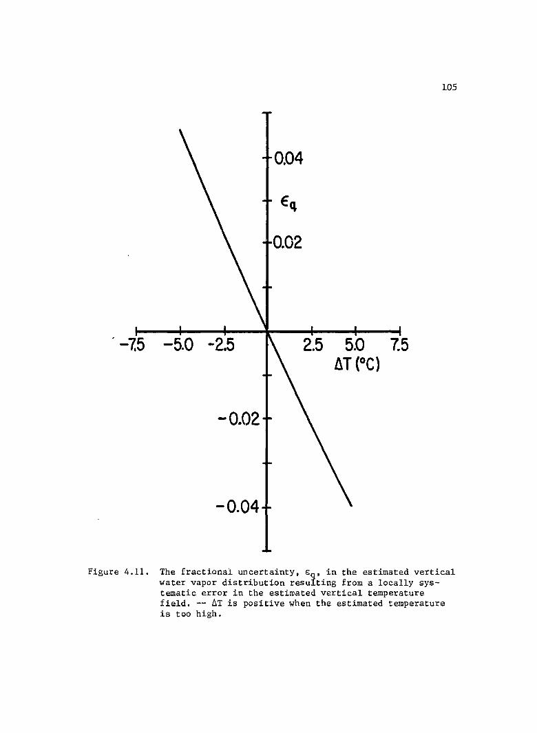
· -7.5
Figure 4.11.
105
7.5
The fractional uncertainty, Eq , in the estimated vertical water vapor distribution resulting from a locally systematic error in the estimated vertical temperature field. -- ~T is positive when the estimated temperature is too high.
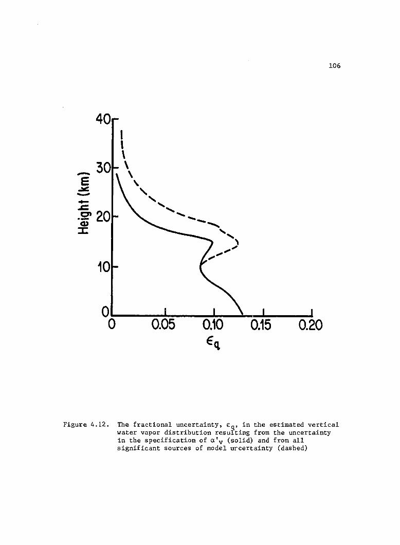
106
40 I , \ \
.....-- \ E ,
-'!I: , -~ , .c " en ' ..... --Q) ..... """" :r: " ,
,," ,,~
10
O~ __ ~~ ____ ~ __ ~. __ I ______ I
o 0.05 0.10 0.15 0.20 Eq
Figure 4.12. The fractional uncertainty, £q' in the estimated vertical water vapor distribution resulting from the uncertainty in the specification of a'v (solid) and from all significant sources of model urcertainty (dashed)
107
Also in Figure 4.12 is shown the estimated maximum likely error
associated with the model. This error includes the effect of the prob-
lem in the specification of a'L and in specifying a single value of
a' which forces the equivalent optical depth predicted by Equation v
4.10 to be the same as that predicted by Equation 4.4.
It can be seen that the magnitude of the possible biasing due
to the specification of a' is at worst comparable to and in general v
much less than the effect of realistic measurement errors shown in
Figure 4.10. Based upon a comparison of Figures 4.10 and 4.12 it is
reasonable to assert that within the stratosphere the model is
effectively not biased.
The final possible source of error is in any failure in the
correlated absorption coefficient assumption. The value of the RMS
spreading of absorption coefficient rank, G, is shown in Figures
3.9a and 3.9b as a function height. Using a two layer model of the
atmosphere and the transmission model of Equation 3.66 it was found
that errors in the effective optical depth calculation for strato-
spheric conditions would be expected to be less than 1% throughout the
stratosphere and less than 0.1% above 20km due to the above assumption.
Therefore the uncertainty in the mixing ratio determination due to the
assumption of the independence of the absorption coefficient rank on
temperature and pressure is negligible.
Three sets of water vapor effective optical depth measurements
have been acquired courtesy of NASA-Langley for 11/29/84 to 11/30/84
over Laramie, Wyoming and Cleve~and, Ohio. These measurements, made
108
as a function of tangent height in increments of 1km were made for a
temperature and pressure distribution measured locally by radiosonde.
Along with the measurements, estimates of the uncertainty in the
effective optical depth were given as were solutions to the three data
sets achieved by an independent inversion technique. The technique
which NASA-Langley employed was the emissivity curve of growth method
described by Weinreb and Neuendorffer (1973).
The results of the data reductions by the iterative method
developed in this chapter are shown in Figures 4.13a, 4.13b and 4.13c
along with the results from the emissivity curve of growth method as
calculated by NASA (Chu, personal communication). There is a good
overall agreement between the two models as the basic trends of the
estimated water vapor profiles by both techniques are quite similar.
Below 16km the two modes of estimation yield results that exhibit no
systematic difference, however, above 16km the iterative reduction
method yields water vapor mixing ratios that average about 10% less
than those determined by the other method. This systematic disagree
ment indicates that either one or both of the techniques is moderately
biased. The RMS difference between the two sets of solutions is
about 8%.
In Figure 4.14 the uncertainty in qn' £q' due to random
measurement errors as determined by Equations 4.27 and 4.25 are shown
for the three example cases. The results are somewhat disappointing
in that the 95% confidence limits average to be 30% of the value of
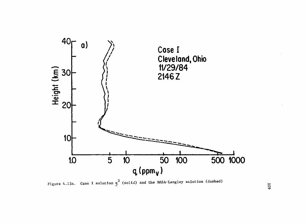
a) i) Case I I
I I
Cleveland Oh" \
"'-"'"
I t1I29/84 ' 10
~ I
...- \l, .s::::.
2146Z
C' I , I I
.:::---:::..."::---- --• I '- I ~J
1.0 5 10 50 100 500 1000 '1 (ppmv)
Figure 4.13a, Case I solution q3 (solid) and the NASA-Langley solution (dashed) I-' a \0
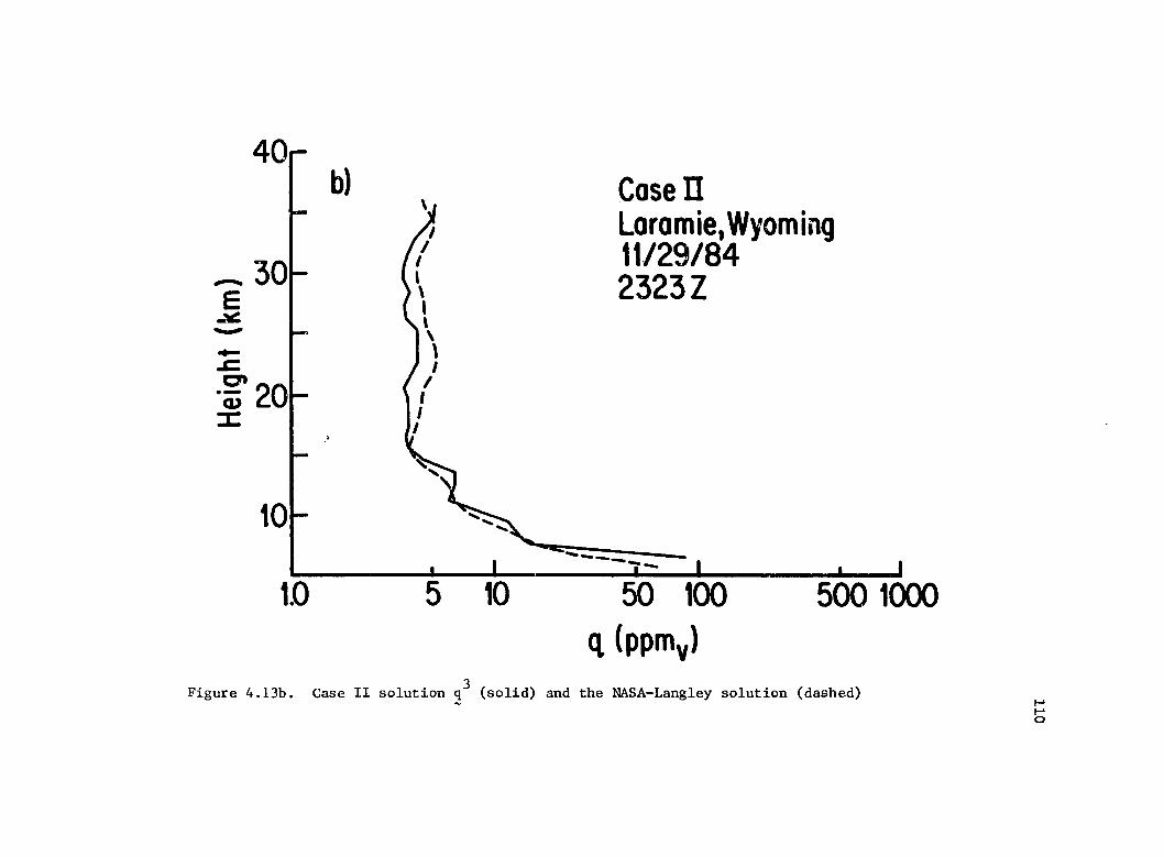
b)
........
.'
1.0 5 10
CaseU Loramie, Wyoming 11/29/84 2323Z
50 100 q (ppmy)
500 1000
Figure 4.13b. Case II solution q3 (solid) and the NASA-Langley solution (dashed) ..... ..... a
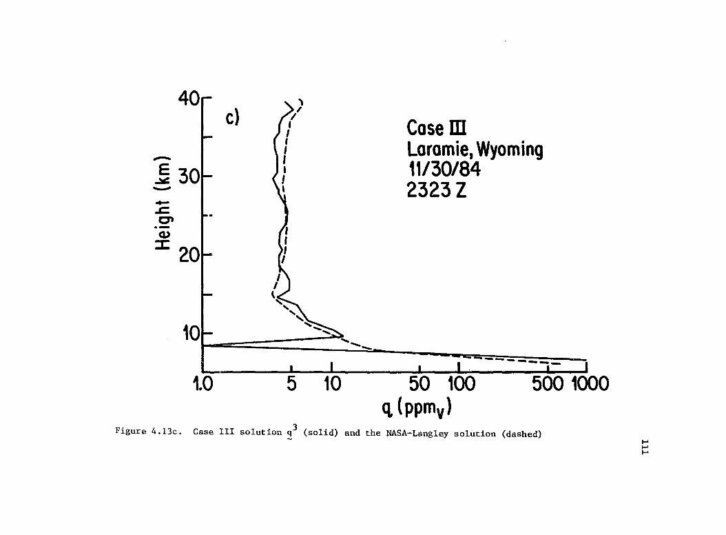
-.... ...-.s= C'
c) / , I , , , I I ,
, , Casem Laramie, Wyoming 11/30/84 2323Z
-------- J I I
1.0 5 10 50 100 500 1000 q, (ppmv)
Figure 4.13c. Case III solution q3 (solid) and the NASA-Langley solution (dashed) I-' I-' I-'
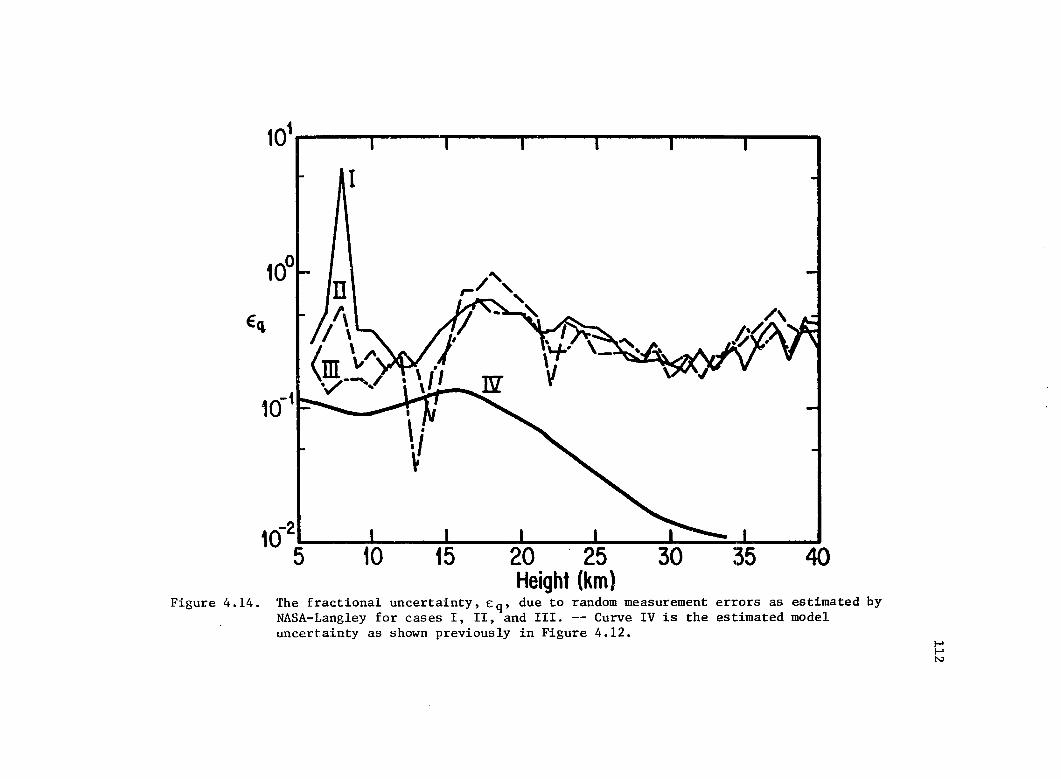
101.~~~_-r--'r--'--.---'---•
I
10°
Eq
-2 10 ' , , 5 10 15 20 25 30 35 40
Height (km) Figure 4.14. The fractional uncertainty, €q' due to random measurement errors as estimated by
NASA-Langley for cases I, II, and III. -- Curve IV is the estimated model uncertainty as shown previously in Figure 4.12.
I-' I-' N
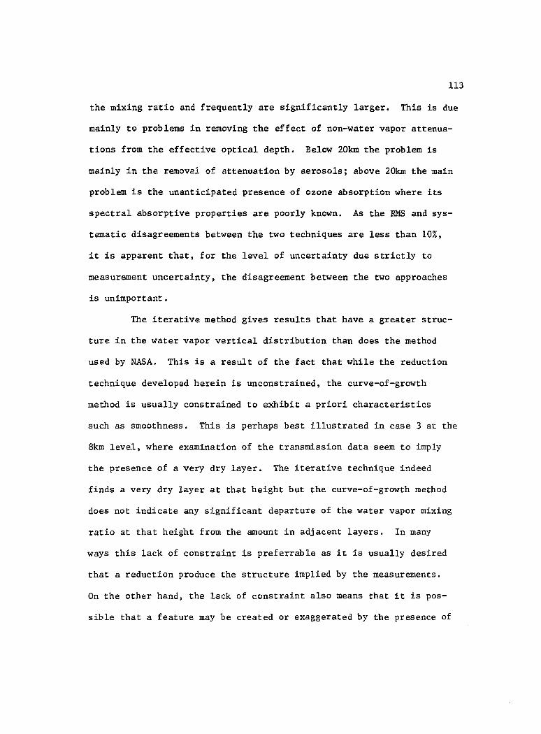
113
the mixing ratio and frequently are significantly larger. This is due
mainly to problems in removing the effect of non-water vapor attenua
tions from the effective optical depth. Below 20km the problem is
mainly in the removal of attenuation by aerosols; above 20km the main
problem is the unanticipated presence of ozone absorption where its
spectral absorptive properties are poorly known. As the RMS and sys
tematic disagreements between the two techniques are less than 10%,
it is apparent that, for the level of uncertainty due strictly to
measurement uncertainty, the disagreement between the two approaches
is unimportant.
The iterative method gives results that have a greater struc
ture in the water vapor vertical distribution than does the method
used by NASA. This is a result of the fact that while the reduction
technique developed herein is unconstrained, the curve-of-growth
method is usually constrained to exhibit a priori characteristics
such as smoothness. This is perhaps best illustrated in case 3 at the
8km level, where examination of the transmission data seem to imply
the presence of a very dry layer. The iterative technique indeed
finds a very dry layer at that height but the curve-of-growth method
does not indicate any significant departure of the water vapor mixing
ratio at that height from the amount in adjacent layers. In many
ways this lack of constraint is preferrab1e as it is usually desired
that a reduction produce the structure implied by the measurements.
On the other hand, the lack of constraint also means that it is pos
sible that a feature may be created or exaggerated by the presence of
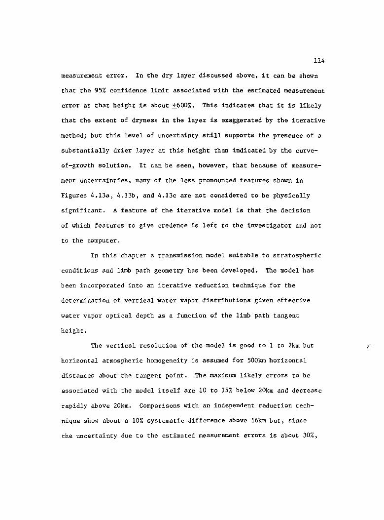
114
measurement error. In the dry layer discussed above, it can be shown
that the 95% confidence limit associated with the estimated measurement
error at that height is about ~OO%. This indicates that it is likely
that the extent of dryness in the layer is exaggerated by the iterative
method; but this level of uncertainty still supports the presence of a
substantially drier Jayer at this height than indicated by the curve
of-growth solution. It can be seen, however, that because of measure
ment uncertainties, many of the less pronounced features shown in
Figures 4.13a, 4,13b, and 4.13c are not considered to be physically
significant. A feature of the iterative model is that the decision
of which features to give credence is left to the investigator and not
to the computer.
In this chapter a transmission model suitable to. stratospheric
conditions and limb path geometry has been developed. The model has
been incorporated into an iterative reduction technique for the
determination of vertical water vapor distributions given effective
water vapor optical depth as a function of the limb path tangent
height.
The vertical resolution of the model is good to 1 to 2km but
horizontal atmospheric homogeneity is assumed for 500km horizontal
distances about the tangent point. The maximum likely errors to be
associated with the model itself are 10 to 15% below 20km and decrease
rapidly above 20km. Comparisons with an independent reduction tech
nique show about a 10% systematic difference above 16km but, since
the uncertainty due to the estimated measurement errors is about 30%,
115
the difference is of little importance. The agreement between the two
solution sets tends to validate each model on the 10 to 20% level.
Overall, the Stieltjes transmission model and the associated
it~rative reduction technique seem to fulfill the requirement of compu
tational efficiency and accuracy. While the level of measurement
uncertainty associated with the SAGE II data perhaps makes even this
level of computational sophistication unjustified, the fundamental
approach has been shown to yield reasonable results and to be a
potentially powerful tool in remote sensing.
CHAPTER 5
SUMMARY AND CONCLUSIONS
A new technique for calculations transmission along
inhomogeneous paths in spectral intervals dominated by molecular line
absorption has been developed for remote sensing applications. It
has been incorporated into a reduction technique that is nu~erically
stable and which produces a unique solution to a set of measured
effective optical depths. The method, as was required. has been
shown to be computationally efficient and accurate.
The technique, which is called the Stieltjes method, has
previously been applied only in an empirical fashion to flux diver
gence calculations which are substantially less sensitive calcula
tions than the ones addressed in chapters III and IV. The first
explicit derivation and formulization of the Stieltjes method has
been presented. The first formal test of the correlated absorption
coefficient assumption showed that the correlation between different
heights in the atmosphere is quite low and this would imply that
the model is invalid. From the derivation of the method, it was
sho~~ that the actual assumption made in the model is that the rank
of the absorption coefficient at any wavenumber is independent of
temperature and pressure. This assumption was shown to be reasonably
valid as it was shown to cause errors no greater than 3% in
116
precipitable water estimates and negligible errors in water vapor
mi~ing ratio estimates for the stratosphere.
117
The numerical integration of the Stieltjes transmission
equation can easily be performed with high precision for homogeneous
and inhomogeneous atmospheres. To simplify the computational pro
blem, model forms of the distribution of absorption coefficient were
derived and a new tecmlique for the determination of the model's
significant parameters was introduced. While there was good overall
agreement between the model g(k) and the true g(k), there was some
degree of difference which found expression in the uncertainty in
the specification of both a.' Land CL "v' The estimated maximum error
in precipitable water estimates resulting from the use of a model
form of g(k) is 8% while in the determination of the water vapor
mixing ratio distribution, it was found to be between 0 and 15%
depending on r.~ight. The maximum error estimated to result from
model assumptions was shown to be no worse than comparable, and in
general much less than, the uncertainty in the solutions introduced
by measurement error. Overall, the technique is nicely capable of
solving the two problems to which it has been applied.
For the cur~ent applications, there is little justification
in further numerical intricacies. However, if the measurement
errors are reduced or the method is applied to a different spectral
applied to a different spectral inter.'al, there are some further
refinements that may be warranted. If the computational facilities
allow, the creation and use of cumulative absorption coefficient
118
distributions by the random-frequency-selection method would eliminate
or greatly reduce the single largest source of error associated with
the method. The other source of error associated with the model is
the correlated absorption coefficient assumption which is ~ signifi-
cant source of error only in the lower atmosphere. A band transmission
function independent of any correlation assumption and for an
inhomogeneous path may be written as
J ! J 000
00 N ! exp[-~ k u J p(k1 , k2' k3 ••• kN) o n=l n n
(5.1)
where p(k1 , k2' k3' ••. kN) is the joint distribution of absorption
coefficient within layers 1 through N. The joint distribution of
absorption coefficient may be written p(~) and p(k1 , k2' k3' ••• , kN)
dk1dk2dk3 ••. dkN is the probability that the ~b50rption coefficient
in layer 1 is between k1 and k1 + dk1 and in layer 2 it is between
k2 and k2 + dk2 ~qd so on through layer N. The correlated absorption
coefficient assumption presumes that p(~) may be written as
where the function f is single valued. By substituting Equation n
(5.2)
5.2 into Equation 5.1, the Stieltjes transmission equation as given
in Equation 2.23 may be produced. It has been shown that the
assumption of rank maintenance that underlies the joint distribution
of absorption coefficient of Equation 5.2 is not completely valid.
It is possible that further study will yield at least an empirical
coorection to p(~) that allows realistic variations of the rank of
the absorption coefficient at a given wavenumber with height.
119
The main strength of the Stieltjes method is that it main
tains many of the characteristics of a line-by-line transmission
calculation. This allows a low cost means of simulating other more
empirical transmission or inversion techniques in order to rigor
ously test their model assumptions and their overall applicability.
For instance, the emissivity curve of growth method is derived for a
nlonochromatic measurement and applied to fairly broad spectral
interval measurement. If it's performance must be tested by line
by-line calculations then the test must be limited in scope but use
of the Stieltje3 method would allow thorough testing of the method
even given limited computing facilities.
LIST OF REFERENCES
Box, M., 1981: Finite Bandwidth and Scattered Light Effects on the Radiometric Determination of Atmospheric Turbidity and the Dolar Constant. App1. Opt., 20, 2215-2219.
Chandrasekhar, S., 1960: Radiative Transfer. Dover Publications, Inc., 393 pp.
Chou, S., and D. Atlas, 1982: Satellite Estimates of Ocean-Air Heat Fluxes During Cold Air Outbreaks. Mon, Wea. Rev., 110, 1434-1450.
Chu, W., 1983: Calculations of Atmospheric Refraction for Spacecraft Remote-Sensing Applications. Appl. Opt., ~, 721-725.
Clough, S., F. Kneizys, L. Rothman, and W. Gallery, 1981: Atmospheric Spectral Transmission and Radiance: FASCODIB. SPIE, 277, 152-166. -
Domoto, G. A., 1974: Frequency Integration for Radiative Transfer Problems Involving Homogeneous Non-Gray Gases: The Inverse Transmission Function. J. Quant. Spectrosc. Radiat. Transfer, 14, 935-942.
Ellsaesser, H., 1983: Stratospheric Water Vapor. J. Geophys, Res., 88, 3897-3906.
Frieden, B. R., 1983: Probability, Statistical Optics, and Data Testing: A Problem Solving Approach. Springer-Verlag, 404 pp.
Gille, J. and R. Ellingson, 1968: Correction of Random Exponential Band Transmissions for Doppler Effects. Appl. Opt., 2, 471-474.
Godson, W. L., 1955a: The Computation of Infrared Transmission by Atmospheric Water Vapor. J. Meteor., 12, 272-284.
Godson, W. L., 1955b: The Computation of Infrared Transmission by Atmospheric Water Vapor, Part II. J. Meteor., 12, 533-535.
Goody, R., 1964: Atmospheric Radiation, Theoretical Basis. Clarendon Press, 436 pp.
120
121
Goody R., 1952: A Statistical Model for Water Vapor Absorption. Quart. J. R. Meteor. Soc., 78, 165-169.
Grad shteyn, I. and I. Ryzhik, 1980: Table of Integrals, Series, and Products. Academic Press, 1160 pp.
Hansen, J., G. Russell, D. Rind, P. Stone, A. Lacis, S. Lebedeff, R. Ruedy, and L. Travis, 1983: Efficient. Three-Dimensional Global Models for Climate Studies: Models I and II. Mon. Wea. Re"., 111, 609-662.
Heicklen, L., 1976: Atmospheric Chemistry. Academic Press, 406 pp.
Kondrat'yev, K. Ya., 1969: Radiation in the Atmosphere. Academic Press, 912 pp.
Kreyszig, E., 1979: Advanced Engineering Mathematics. John Wiley and Sons, 939 pp.
Lacis, A. A., and J. E. Hansen, 1979: A Parameterization for the Absorption of Solar Radiation in the Earth's Atmosphere. J. Atmos. Sci., 31, 118-133.
Liou, K., 1974: On the Radiative Properties of Cirrus in the Window Region and Their Influence on Remote Sensing of the Atmosphere. J. Atmos. Sci., 31, 522-532.
Malkmus, W., 1967: Random Lorentz Band Model with Exponential-Tailed S-1 Line Intensity Distribution Function. J. Opt. Sci. Amer., 51, 323-329.
Mankin, W. G., 1979: Fourier Transform Method for Calculating the Transmittance of Inhomogeneous Atmospheres. Appl. Opt., 18, 3426-3433.
McClatchey, R., W. Benedict, S. Clough, D. Furch, R. Calfis, K. Fox, L. Rothman, and J. Garing, 1973: AFCRL Atmospheric Absorption Line Parameters Compilation. Environ. Res. Pop. No. 434, AFCRL-TR-0096, 80 pp.
Rodgers, C. D., and C. D. Walshaw, 1966: The Computation of Infrared Cooling Rate in Planetary Atmospheres. Quart. J. R. Meteor; Soc., 92, 67-92.
Russell, J., J. Gille, E. Remsberg, L. Gordley, ~. Bailey, H. Fischer, A. Girard, S. R. Drayson, W. Evans, and J. Harris, 1984: Validation of Water Vapor Results Measured by the Limb Infrared Monitor of the Stratosphere Experiment on NIMBUS 7. J. Geophys. Res., 89, 5115-5124.
Spencer-Gregory, H., and E. Rourke, 1957: Hygrometry. Pitman Publishing Corp., 254 pp.
Stae1in, D., K. Kunzi, R. Pettyjohn, R. Poon, R. Wilcox, and J. Waters, 1976: Remote Sensing of Atmospheric Water Vapor and Liquid Water With the NIMBUS 5 Microwave Spectrometer. J. App1. Meteor., J.5, 1204-1214.
Stark, P., 1970: Introduction to Numerical Methods. MacMillan Publishing Co., Inc., 334 pp.
Taylor, A. and W. Mann, 1972: Advanced Calculus. John Wiley and Sons, 714 pp.
1/2
Thomason, L. W., B. M. Herman, R. M. Scotland, and J. A. Reagan, 1982: Extraterrestrial Solar Flux Measurement Limitations due to a Beer's Law Assumption and Uncertainty in Local Time. App1. Opt., 21, 1191-1195.
Twomey, S., 1977: Introduction to the Mathematics of Inversion in Remote Sensing and Indirect Measurements. Elsevier Scientific Publishing Company, 243 pp.
U.S. Standard Atmosphere, 1976: NOAA-SIT 76-1562, U.S. Government Printing Office. 227 pp.
Wang, W., and P. B. Ryan, 1983: Overlapping Effect of Atmospheric H20, CO2, and 03 on the CO2 Radiative Effect. Tel1us, 358, 81-91.
Weinreb, M., and A. Neuendorffer, 1973: Method to Apply HomogeneousPath Transmittance Models to Inhomogeneous Atmospheres. J. Atmos. Sci., 30, 662-666.