Embed Size (px)
Citation preview
ON CONSISTENT KALUZA-KLEIN-PAULI REDUCTIONS
A Dissertation
by
ARASH AZIZI
Submitted to the Office of Graduate and Professional Studies ofTexas A&M University
in partial fulfillment of the requirements for the degree of
DOCTOR OF PHILOSOPHY
Chair of Committee, Christopher N. PopeCommittee Members, Ergin Sezgin
Teruki KamonStephen A. Fulling
Head of Department, Grigory Rogachev
August 2018
Major Subject: Physics
Copyright 2018 Arash Azizi
ABSTRACT
Kaluza-Klein dimensional reduction is an indispensable ingredient of the theoretical physics,
since, M-theory and superstring theories are consistent in eleven and ten dimensions and thus, to
make a connection to our four-dimensional space-time physics, it is crucial to use this mechanism.
Dimensional reduction on a general coset space such as a sphere, introduced by Pauli, is more sub-
tle that that of a group manifold reduction, introduced by DeWitt, including the circle reduction of
Kaluza and Klein. While there is a group-theoretic argument for the consistency of the latter, there
is no such an argument for the former, hence, besides the exceptional cases, all Pauli reductions
may be inconsistent.
We study an uplift ansatz for two specific truncations of gauged STU supergravity. This theory
itself is an important truncation of the renowned N = 8, gauged SO(8) supergravity in four
dimensions. We consider two truncations of the former theory, named as 3+1 and 2+2, due to the
way of truncations of their gauge fields. We find the uplift ansätze for the metric and the four-form
field strength in these cases.
We consider two theories and explore the possibility of their consistent Pauli S2 reductions.
First, minimal supergravity in five dimensions, and second, the Salam-Sezgin theory. We use the
Hopf reduction technique in both cases, and by that, we show while it is not possible to perform
a consistent reduction of the former, there is a consistent Pauli reduction of the latter, and by this
construction, we can recover the result of Gibbons-Pope in 2003. In other words, we can provide
a group theoretical argument for their work. To make the latter case happen, we find a new higher
dimensional origin for the Salam-Sezgin theory, at least in the bosonic sector.
ii
DEDICATION
To my mother, my father,
To Sophia,
To Sahar.
iii
ACKNOWLEDGMENTS
First and foremost, I would like to thank my advisor, Chris Pope, for all of his support, guide,
help, understanding and care. He is one of the pioneers of the Kaluza-Klein theory. His enormous
patience to elaborate all details of somewhat trivial points to me is of great appreciation. His gen-
erous financial support, especially during the dark days, will not be forgotten. Also, I enjoyed his
unique way of teaching with detailed lecture notes in several courses including general relativity.
I would like to thank Ergin Sezgin for several reasons. I learned supersymmetry and supergrav-
ity mostly from two important courses he taught in the department. Especially, he helped me a lot
during the intense discussions we have had about the fermionic part of my work. He is a brilliant
and very passionate physicist and I have been enjoying his comments on our high energy theory
weekly seminars. The Salam-Sezgin theory, which is an important part of my work, constructed
by him and Salam in 1984.
Special thanks to Teruki Kamon and Stephen Fulling for accepting to be part of my committee
members. I really appreciate their comments about the dissertation.
I would like to thank Katrin Becker, Melanie Becker, Bhaskar Dutta and Dimitri Nanopoulos
for wonderful courses they taught in the department. Also, I am grateful to Daniel Butter for very
stimulating discussions.
I would like to thank my collaborators Chris Pope, Hadi and Mahdi Godazgar.
Many thanks to William Bassichis, Barun Dhar, Emanuela Ene, Tatiana Erukhimova, Lewis
Ford, Robert Webb and Michael Weimer for wonderful discussions especially about how to teach
physics.
I am grateful to Marlan Scully and Girish Agarwal to let me stay in the office which belongs to
IQSE.
During my Ph.D. I have been enjoying good discussions about physics and beyond with nu-
merous colleagues and friends. They are including, Charles Altuzarra, Elham Azadbakht, Amin
Barzegar, Aysan Bahari, Steven Clark, Nader Ghassemi, Sunny Guha, Shayan Hemmatiyan,
iv

Esteban Jimenez, Surya Kanumilli, Jie Li, Zhijin Li, William Linch, Mehmet Ozkan, Navid
Rajil, Junchen Rong, Andrew Royston, Saeideh Shahrokh, Ali Sirusi, Ansam Talib, Yaodong
Zhu and especially Yusef Maleki.
I also appreciate Sherree Kessler, Mary Louise Sims, Michelle Sylvester, and Heather Walker
from the physics department, for their help.
Last but not least, I would like to thank my family. My father taught me mathematics when I
was just three and always encourages me to follow my dreams. My mother supports me with
endless love. My brother Soroosh, has been helpful and supportive for me. My sister in law
Sara, helps my family and me, especially in past two years enormously. My wife Sahar is giving
me love, joy, happiness and calmness. I am a lucky man to have her in my life. My little daughter
Sophia, is the sweetest kid ever! Her laugh, love and joyful life is the best gift my wife gave to
me.
v
CONTRIBUTORS AND FUNDING SOURCES
Contributors
This work was supported by a dissertation committee consisting of Professor Christopher N.
Pope, Professor Ergin Sezgin, Professor Teruki Kamon of the Department of physics, and Professor
Stephen A. Fulling of the Department of mathematics of Texas A&M University.
All work conducted for the dissertation was completed by Arash Azizi independently.
vi
TABLE OF CONTENTS
Page
ABSTRACT . . . . . . . . . . . . . . . . . . . . . . . . . . . . . . . . . . . . . . . . . . . . . . . . . . . . . . . . . . . . . . . . . . . . . . . . . . . . . . . . . . . . . . . . . ii
DEDICATION . . . . . . . . . . . . . . . . . . . . . . . . . . . . . . . . . . . . . . . . . . . . . . . . . . . . . . . . . . . . . . . . . . . . . . . . . . . . . . . . . . . . . . . iii
ACKNOWLEDGMENTS . . . . . . . . . . . . . . . . . . . . . . . . . . . . . . . . . . . . . . . . . . . . . . . . . . . . . . . . . . . . . . . . . . . . . . . . . . iv
CONTRIBUTORS AND FUNDING SOURCES . . . . . . . . . . . . . . . . . . . . . . . . . . . . . . . . . . . . . . . . . . . . . . . . . vi
TABLE OF CONTENTS . . . . . . . . . . . . . . . . . . . . . . . . . . . . . . . . . . . . . . . . . . . . . . . . . . . . . . . . . . . . . . . . . . . . . . . . . . . vii
1. INTRODUCTION. . . . . . . . . . . . . . . . . . . . . . . . . . . . . . . . . . . . . . . . . . . . . . . . . . . . . . . . . . . . . . . . . . . . . . . . . . . . . . . 1
1.1 Historical remarks . . . . . . . . . . . . . . . . . . . . . . . . . . . . . . . . . . . . . . . . . . . . . . . . . . . . . . . . . . . . . . . . . . . . . . . . 11.2 DeWitt and Pauli reductions . . . . . . . . . . . . . . . . . . . . . . . . . . . . . . . . . . . . . . . . . . . . . . . . . . . . . . . . . . . . . . 31.3 Three revivals of the dimensional reduction . . . . . . . . . . . . . . . . . . . . . . . . . . . . . . . . . . . . . . . . . . . . 51.4 Dissertation outline . . . . . . . . . . . . . . . . . . . . . . . . . . . . . . . . . . . . . . . . . . . . . . . . . . . . . . . . . . . . . . . . . . . . . . . 6
2. REVIEW OF THE KALUZA-KLEIN REDUCTION . . . . . . . . . . . . . . . . . . . . . . . . . . . . . . . . . . . . . . . . 9
2.1 The Klein-Gordon case . . . . . . . . . . . . . . . . . . . . . . . . . . . . . . . . . . . . . . . . . . . . . . . . . . . . . . . . . . . . . . . . . . . 92.2 The Kaluza-Klein circle reduction . . . . . . . . . . . . . . . . . . . . . . . . . . . . . . . . . . . . . . . . . . . . . . . . . . . . . . . 10
2.2.1 The metric ansatz . . . . . . . . . . . . . . . . . . . . . . . . . . . . . . . . . . . . . . . . . . . . . . . . . . . . . . . . . . . . . . . . 102.2.2 The vector potential ansatz . . . . . . . . . . . . . . . . . . . . . . . . . . . . . . . . . . . . . . . . . . . . . . . . . . . . . . 13
3. THE EMBEDDING OF TRUNCATED GAUGED STU SUPERGRAVITIES IN 11 DI-MENSIONS . . . . . . . . . . . . . . . . . . . . . . . . . . . . . . . . . . . . . . . . . . . . . . . . . . . . . . . . . . . . . . . . . . . . . . . . . . . . . . . . . . . . . 15
3.1 Introduction . . . . . . . . . . . . . . . . . . . . . . . . . . . . . . . . . . . . . . . . . . . . . . . . . . . . . . . . . . . . . . . . . . . . . . . . . . . . . . . 153.2 3 + 1 Truncation of gauged STU supergravity . . . . . . . . . . . . . . . . . . . . . . . . . . . . . . . . . . . . . . . . . . 17
3.2.1 The embedding of the metric . . . . . . . . . . . . . . . . . . . . . . . . . . . . . . . . . . . . . . . . . . . . . . . . . . . . 183.2.1.1 The CP2 geometry . . . . . . . . . . . . . . . . . . . . . . . . . . . . . . . . . . . . . . . . . . . . . . . . . . . . 183.2.1.2 Obtaining the metric ansatz in terms of CP2 geometry . . . . . . . . . . . . . 18
3.2.2 The embedding of the four-form . . . . . . . . . . . . . . . . . . . . . . . . . . . . . . . . . . . . . . . . . . . . . . . . 213.2.2.1 Finding the Lagrangian . . . . . . . . . . . . . . . . . . . . . . . . . . . . . . . . . . . . . . . . . . . . . . . 24
3.3 2 + 2 Truncation of gauged STU supergravity . . . . . . . . . . . . . . . . . . . . . . . . . . . . . . . . . . . . . . . . . . 253.3.1 The embedding of the metric . . . . . . . . . . . . . . . . . . . . . . . . . . . . . . . . . . . . . . . . . . . . . . . . . . . . 253.3.2 The embedding of the four-form . . . . . . . . . . . . . . . . . . . . . . . . . . . . . . . . . . . . . . . . . . . . . . . . 283.3.3 Finding the bosonic Lagrangian . . . . . . . . . . . . . . . . . . . . . . . . . . . . . . . . . . . . . . . . . . . . . . . . . 31
vii
4. ON THE PAULI REDUCTION OF MINIMAL SUPERGRAVITY IN FIVE DIMEN-SIONS . . . . . . . . . . . . . . . . . . . . . . . . . . . . . . . . . . . . . . . . . . . . . . . . . . . . . . . . . . . . . . . . . . . . . . . . . . . . . . . . . . . . . . . . . . . 32
4.1 Introduction . . . . . . . . . . . . . . . . . . . . . . . . . . . . . . . . . . . . . . . . . . . . . . . . . . . . . . . . . . . . . . . . . . . . . . . . . . . . . . . 324.2 S1 reduction of minimal D = 6 supergravity. . . . . . . . . . . . . . . . . . . . . . . . . . . . . . . . . . . . . . . . . . . . 33
4.2.1 A Kaluza-Klein circle reduction to 5D . . . . . . . . . . . . . . . . . . . . . . . . . . . . . . . . . . . . . . . . . 354.2.2 Finding the bosonic Lagrangian in 5D . . . . . . . . . . . . . . . . . . . . . . . . . . . . . . . . . . . . . . . . . . 364.2.3 Truncations to minimal supergravity in 5D . . . . . . . . . . . . . . . . . . . . . . . . . . . . . . . . . . . . 38
4.3 SU(2) DeWitt reduction from D = 6 to D = 3 . . . . . . . . . . . . . . . . . . . . . . . . . . . . . . . . . . . . . . . . . 384.3.1 The ansätze for an SU(2) group manifold reduction. . . . . . . . . . . . . . . . . . . . . . . . . . . 394.3.2 SU(2) as a Hopf fibration . . . . . . . . . . . . . . . . . . . . . . . . . . . . . . . . . . . . . . . . . . . . . . . . . . . . . . . 41
4.4 Impossibility of the Pauli reduction of 5D minimal supergravity . . . . . . . . . . . . . . . . . . . . . . 49
5. AN ALTERNATIVE M-THEORY ORIGIN OF THE SALAM-SEZGIN THEORY . . . . . . . 51
5.1 Introduction . . . . . . . . . . . . . . . . . . . . . . . . . . . . . . . . . . . . . . . . . . . . . . . . . . . . . . . . . . . . . . . . . . . . . . . . . . . . . . . 515.2 ObtainingN = 2 gauged SO(4) fromN = 4 gauged SO(5) supergravity in seven
dimensions . . . . . . . . . . . . . . . . . . . . . . . . . . . . . . . . . . . . . . . . . . . . . . . . . . . . . . . . . . . . . . . . . . . . . . . . . . . . . . . . 535.2.1 Review of N = 4 gauged SO(5) supergravity in 7D . . . . . . . . . . . . . . . . . . . . . . . . . . 535.2.2 The Inönü-Wigner group contraction limit of the SO(5) . . . . . . . . . . . . . . . . . . . . . 575.2.3 Review of N = 2 gauged SO(4) supergravity in seven dimensions . . . . . . . . . 575.2.4 Towards a Wick rotated supergravity in seven dimensions . . . . . . . . . . . . . . . . . . . . 615.2.5 Why the Wick rotated theory is necessary to study the fermionic sector? . . . . 63
5.3 The Kaluza-Klein circle reduction to six dimensions: bosonic sector . . . . . . . . . . . . . . . . . 645.3.1 The ansätze for gauge potentials . . . . . . . . . . . . . . . . . . . . . . . . . . . . . . . . . . . . . . . . . . . . . . . . 655.3.2 The Chern-Simons term in seven dimensions . . . . . . . . . . . . . . . . . . . . . . . . . . . . . . . . . . 675.3.3 The bosonic equations of motion . . . . . . . . . . . . . . . . . . . . . . . . . . . . . . . . . . . . . . . . . . . . . . . . 685.3.4 The bosonic truncations. . . . . . . . . . . . . . . . . . . . . . . . . . . . . . . . . . . . . . . . . . . . . . . . . . . . . . . . . . 705.3.5 The supersymmetry transformations? . . . . . . . . . . . . . . . . . . . . . . . . . . . . . . . . . . . . . . . . . . . 72
5.4 Final remarks . . . . . . . . . . . . . . . . . . . . . . . . . . . . . . . . . . . . . . . . . . . . . . . . . . . . . . . . . . . . . . . . . . . . . . . . . . . . . . 72
6. PAULI S2 REDUCTION OF THE SALAM-SEZGIN THEORY . . . . . . . . . . . . . . . . . . . . . . . . . . . . 74
6.1 Introduction . . . . . . . . . . . . . . . . . . . . . . . . . . . . . . . . . . . . . . . . . . . . . . . . . . . . . . . . . . . . . . . . . . . . . . . . . . . . . . . 746.2 Truncation of N = 2 gauged SO(2, 2) supergravity in seven dimensions . . . . . . . . . . . . 75
6.2.1 Pass to a non-compact SO(2, 2) gauging . . . . . . . . . . . . . . . . . . . . . . . . . . . . . . . . . . . . . . . 766.2.2 Truncation of SO(2, 2) half maximal theory in seven dimensions . . . . . . . . . . . . 76
6.3 The Kaluza-Klein circle reduction down to six dimensions . . . . . . . . . . . . . . . . . . . . . . . . . . . . 776.3.1 The bosonic truncations in six dimensions . . . . . . . . . . . . . . . . . . . . . . . . . . . . . . . . . . . . . 78
6.4 DeWitt SU(2) reduction from 7D theory . . . . . . . . . . . . . . . . . . . . . . . . . . . . . . . . . . . . . . . . . . . . . . . 796.5 SU(2) as a U(1) Hopf fibration over S2 . . . . . . . . . . . . . . . . . . . . . . . . . . . . . . . . . . . . . . . . . . . . . . . . 80
6.5.1 Imposing the six-dimensional truncations . . . . . . . . . . . . . . . . . . . . . . . . . . . . . . . . . . . . . . 816.5.2 Consistency of the ansatz . . . . . . . . . . . . . . . . . . . . . . . . . . . . . . . . . . . . . . . . . . . . . . . . . . . . . . . 83
7. CONCLUSION AND OUTLOOK . . . . . . . . . . . . . . . . . . . . . . . . . . . . . . . . . . . . . . . . . . . . . . . . . . . . . . . . . . . . . 88
viii
REFERENCES . . . . . . . . . . . . . . . . . . . . . . . . . . . . . . . . . . . . . . . . . . . . . . . . . . . . . . . . . . . . . . . . . . . . . . . . . . . . . . . . . . . . . . 93
APPENDIX A. FINDING THE FIELD RE-DEFINITIONS. . . . . . . . . . . . . . . . . . . . . . . . . . . . . . . . . . . . . 98
APPENDIX B. FINDING THE HODGE-DUALITY RELATION WITH A SPHERICALCONSTRAINT . . . . . . . . . . . . . . . . . . . . . . . . . . . . . . . . . . . . . . . . . . . . . . . . . . . . . . . . . . . . . . . . . . . . . . . . . . . . . . . . . . 100
B.1 The notation . . . . . . . . . . . . . . . . . . . . . . . . . . . . . . . . . . . . . . . . . . . . . . . . . . . . . . . . . . . . . . . . . . . . . . . . . . . . . . . 100B.2 The Hodge-dual on a sphere. . . . . . . . . . . . . . . . . . . . . . . . . . . . . . . . . . . . . . . . . . . . . . . . . . . . . . . . . . . . . . 102
ix
1. INTRODUCTION
1.1 Historical remarks
One of the most important and deepest unanswered questions in the history of science is finding
a unique scheme where all forces of nature can be combined to the elegant theory with a beautiful
underlying mathematical structure. The quest for such a “Final Theory” has been initiated mostly
by Albert Einstein, especially when he eventually obtained the final form of general relativity in
November 1915. Right after that, he started a long journey of investigation to find a unification
of the gravity in form of his general relativity and Maxwell’s electromagnetism, the only known
forces at that time. The exploration for such a theory has not been successful during his life time.
However, several brilliant ideas emerged either by himself or by other physicists.
One of the most striking ideas aiming a unification of all forces introduced by Nordström [1]
in 1914, even one year before the completion of general relativity, known as the dimensional
reduction. However this work had been ignored by community for long time. Five years later,
Theodor Kaluza, inspired by a work of Hermann Weyl in 1918, found the same scheme. The
main idea of the dimensional reduction is as follows. Considering pure gravity in five space-time
dimensions and assuming the fifth dimension is compactified on a small circle, one can obtain
gravity and electromagnetism along with a scalar field and an infinite tower of massive fields in
four dimensions. A natural unification of gravity and electromagnetism has been achieved! Kaluza
sent the draft of his paper to Einstein, and while Einstein found out his theory “startling”, he did
not submit the paper to the Prussian Academy for two years [2].
Nordström had developed his own version of gravity, know as scalar gravity, and hence, his
dimensional reduction is different with that of Kaluza. He wrote the higher dimensional Maxwell
vector potential as a combination of the four dimensional vector potential, corresponding to elec-
tromagnetic vector potential, and a scalar field describes his scalar gravity. It is remarkable that
he introduced exactly the same ansatz as it is written today for a vector field. Therefore, his
1
five-dimensional Lagrangian is a pure Maxwell one and after dimensional reduction he obtained
four-dimensional Maxwell electromagnetism and a kinetic scalar term for “gravity”.
Kaluza in his published work [3] in 1921, like Nordström assumed “cylinder condition” , mean-
ing that all fields of the four-dimensional theory are independent of the fifth dimension [2]. In other
words, he implicitly discarded an infinite tower of massive fields. The crucial issue of the consis-
tency then shall be arisen here, i.e. whether a truncation of massive fields is consistent or not. As
we will see later, in the special case of the circle reduction, the case where they studied, this con-
sistency is guaranteed by a simple group-theoretical argument, however, for most of “non-trivial”
dimensional reductions, such a simple test does not exist. Moreover, Kaluza considered just the
linearized level of equations of motion, therefore all of the complications may arise as a result of
considering the highly non-linear nature of the Einstein equations, shall not be addressed by this
consideration.
Klein in 1926 [4] improved the program by considering the full non-linear theory, and by the as-
sumption of the cylinder condition, he could find out pure Einstein gravity in five dimensions gives
rise to Einstein gravity, Maxwell electromagnetism and a scalar in four dimensions. Of course,
the latter field is not a desirable choice for him since there was no known scalar field at that time.
Therefore, he assumed the g55 component of the metric which is proportional to the scalar field, is
constant, and hence the scalar field can be discarded. If just the Lagrangian would be considered,
there is no inconsistency in discarding the scalar field has been arisen. However, the modern crite-
rion for the consistency of the reduction ansatz, pioneered by the work of Duff, Nilsson, Pope and
Warner in 1984 [5], is based on the equations of motion rather than the Lagrangian.
A consistent dimensional reduction is defined as follows. An initial (D+n)-dimensional theory
can be compactified on a compact n-dimensional internal manifold. One can find a Fourier expan-
sion of the D-dimensional theory in terms of the internal manifold harmonics, however, retaining
all of an infinite tower of fields is not essentially interested. Henceforth, one needs to truncate
an infinite number of fields and retain just finite number of them, named ansatz. Especially, one
needs to keep the bosonic fields which express the isometry group of the internal manifold. The
2
criterion for the consistency of an ansatz is as follows. Upon inserting the ansatz in the higher
dimensional equations of motion, due to the conspiracies between several fields, the ones depend
upon the internal manifold cancel out of the equations and the remaining equations shall be those
of the D-dimensional space-time. Specifically, the retaining fields should not be the sources for
discarding ones. In that sense, discarding the scalar field, as Klein considered, is not consistent,
since vanishing R55 in five dimensions implies the Maxwell field strength is a source term for the
scalar field and discarding the latter should be accompanied by discarding the former, i.e. no more
unification shall be achieved.
Now, the question is, finding a general mechanism to construct the consistent reductions. This
is, in general, a very non-trivial question. In fact, besides reductions which their consistency is
guaranteed by a group-theoretic argument, there is no known litmus test to check the consistency
of a reduction. The only way is calculating the higher dimensional equations of motion as we have
just emphasized.
1.2 DeWitt and Pauli reductions
One may classify general dimensional reductions in two categories of DeWitt ( group manifold)
and Pauli (coset) reductions. The former was studied first by Bryce DeWitt in 1963 [6] and then
named DeWitt reduction in [7]. The internal space in this case is a group manifold. Then one can
construct fields which are invariant under the left (or right) action of the group. In other words,
one can easily show U−1 dU , where U is an element of the group manifold, is invariant under the
transformation U → GU , where G is a global rigid element of the group. Therefore, U−1 dU is
invariant under the left action of the group, or the latter is a singlet under the left action of the
group GL. Then if one writes U−1 dU = σa Ta, where T a are the generators of the algebra, hence
σa may be labeled as left-invariant one-forms. Similarly, dU U−1 is invariant under the right action
of the group, i.e. U → UG, and it is a singlet under GR
Having said the above, let us consider the group manifold reduction. Assume an ansatz is
written in terms of the left-invariant fields (or equivalently the right-invariant ones). In other words,
one may retain the singlets under the left action of the isometry group, GL and discard all other
3
fields. Then, one can divide all higher dimensional equations of motion, which are written in terms
of the lower dimensional fields, into two parts: a part includes all terms which are singlets of the
group GL, and the other part involves non-singlet ones. Since the product of all singlets is again
a singlet of the group, by truncating all non-singlet fields to zero, all equations of the latter part
actually are trivially satisfied. There is no danger for surviving fields (i.e. singlets under GL)
to be sources for vanishing ones (i.e. non-singlets under GL). This is why the consistency of a
reduction on a group manifold G is guaranteed by a group-theoretic argument. Note that since a
circle S1 or more general a torus T n are both group manifolds ( U(1) and U(1)n respectively), then
the consistency of Kaluza and Klein original example of a circle S1, or a torus T n reductions are
guaranteed by a group-theoretic argument.
The first coset reduction was investigated by Wolfgang Pauli in an unpublished work in 1953
[2]. He unsuccessfully, attempted to find an S2 reduction of pure Einstein gravity in six dimensions,
while keeping the non-Abelian SO(3) Yang-Mills fields. It is clear now, to obtain a consistent S2
reduction of six-dimensional theory, one needs to start from a supergravity theory, instead of a pure
gravity which Pauli considered. The coset reduction was named Pauli reduction in [7].
In contrast to the DeWitt case, there is no group-theoretical argument applicable to the Pauli
reduction. As a matter of fact, almost all Pauli reductions are inconsistent, however there are ex-
ceptional cases where the Pauli reductions are consistent. Hence, the important question becomes
finding a deeper understanding of why such “miraculous” reductions exist. The main examples
of consistent Pauli reductions include of the renowned S7 reduction of eleven-dimensional super-
gravity of deWit and Nicolai [11] and later [12], S4 reduction of eleven-dimensional supergrav-
ity [13], [14] and [15], the Pauli consistent reduction of type IIB supergravity on S5 in [16], and
the Pauli reduction of the bosonic string on a group manifold G where the the full isometry group
of G×G is retained in [17].
One may ask since a DeWitt reduction can be constructed in an algorithmic method, why
one has to consider the Pauli reductions. First of all, since the isometry group of the bosonic
gauge fields of the lower-dimensional theory is the same as that of the internal manifold, hence to
4
obtain a specific isometry group, a Pauli reduction needs a higher dimensional theory with smaller
dimensions in compare with a DeWitt one. In other words, assuming the lower d-dimensional
theory has a gauge group of G, in the higher D-dimensional theory, D = d + dimG − dimH in
the Pauli reduction on the coset G/H , whereas D = d + dimG in the DeWitt reduction on the
group manifold G. Hence this is somewhat more “economical” way of obtaining the Yang-Mills
in the lower-dimensional theory. Secondly, the mere existence of these reductions motivates us to
investigate their underlying mathematical structure and it may lead us to new aspects, such as the
generalized geometry, which will be addressed briefly later.
1.3 Three revivals of the dimensional reduction
The dimensional reduction had not played a central role in the theoretical physics after its
birth in 1910s until 1970s. However, it has been revived in 1970’s and 1980’s because of the
constructions of supergravities in dimensions higher than four and especially the fact that su-
perstring theories are consistent in ten space-time dimensions. Then to connect these theories
to our four-dimensional space-time, the dimensional reduction is the best tool and technique.
Therefore, in early 1980s, this subject was extensively studied and interesting results were ob-
tained [5, 11, 18–22]. This is the first revival of the program.
The second revival of the dimensional reduction started in late 1997 when Juan Maldacena
made a conjecture about a correspondence between a gravity theory in an anti-de Sitter space and
a conformal field theory on its boundary [23–25]. The prominent example of this correspondence
is type IIB superstring theory on AdS5 × S5 and N = 4 super Yang-Mills on its four dimensional
boundary. Motivated by this example, there was a notable amount of researches conducted to
understand the non-linear structure of a reduction of a higher dimensional theory on a general coset
space like sphere [27–30]. For instance, the Pauli S4 reduction of eleven-dimensional supergravity
was constructed in [13, 14].
The third revival of this program has been started in past few years. There has been an intense
research program known as generalized geometry, where it aims to understand the different dual-
ities of string theory better. This aim can be achieved by assuming the internal manifold has the
5
same dimensions as number of the adjoint representation of the underlying symmetry group of the
theory. Furthermore, by imposing the section constraint on the theory, it makes the hidden sym-
metries of a theory manifest. Within this framework, there is a generalized Scherk-Schwarz [19]
mechanism, where it is possible to have a systematic way of construction of the Kaluza-Klein
ansatz. [31,32] However, there are two issues related to this program. Firstly, the ansatz it is found
by this method is not very practical and one needs to find out a more feasible ansatz, and more
importantly, it is not obvious how to incorporate the fermions in this program. Therefore, with-
out inclusion of the fermions, the Kaluza-Klein ansatz will not address the crucial concept of the
supersymmetry. There are several examples of consistent Kaluza-Klein construction of a bosonic
sector of a theory, however, the construction becomes inconsistent after inclusion of the fermions.
In fact, in our alternative M-theory origin of the Salam-Sezgin theory which will be addressed
shortly, one observes that while it is somewhat an easy task to construct the bosonic truncations, it
is very difficult to find a consistent truncations of the fermionic fields.
1.4 Dissertation outline
This dissertation organizes as follows. In chapter 2, we review the Kaluza-Klein theory by a
toy example of the Klein-Gordon scalar field. Also, a circle reduction shall be addressed in this
chapter. The bosonic Lagrangian and equations of motion will be discussed and it will be shown
that discarding the dilaton field results from the circle reduction is inconsistent with retaining the
Maxwell field.
In chapter 3, we will find the embedding of two specific truncations of the STU supergravity in
eleven dimensions. The latter theory is a maximal Abelian (i.e. U(1)4) sub-group of the renowned
four-dimensional N = 8, SO(8) gauge supergravity, and has an essential role in study of black
holes in four dimensions. We will study two different truncations of this theory, i.e. 3 + 1 and
2 + 2, where besides a graviton, two gauge fields and a dilaton and an axion survive in these two
scenarios. We will find out the embedding eleven-dimensional metric and four-form field strength
in the above mentioned truncations.
In chapter 4, we will raise a question of the possibility of consistent Pauli S2 reduction of min-
6
imal five-dimensional supergravity. The motivation for this study comes from the similarity be-
tween the latter theory’s bosonic Lagrangian and that of eleven-dimensional supergravity. Hence,
since there are consistent Pauli S4 and S7 reductions of eleven-dimensional supergravity, one may
conjecture a consistent Pauli S2 reduction of five-dimensional minimal supergravity exists. We
will show, using the Hopf reduction technique, there is no such a consistent Pauli reduction in this
case.
The Einstein-Maxwell N = (1, 0) six-dimensional theory, known as the Salam-Sezgin the-
ory [36], will be subject of two chapters 5 and 6. The latter theory has a supersymmetric four-
dimensional Minkowski4 × S2 vacuum solution, then one may wonder about the possibility of
consistent S2 Pauli reduction of it. This reduction found in 2003 by Gibbons and Pope [38], how-
ever, one does not have an understanding of why this reduction works. Using the Hopf reduction
technique, we have been able to find a group-theoretic understanding of this reduction. For this
purpose, the Salam-Sezgin theory should be derived from a seven-dimensional theory. This has
been done in [39], however, the Kaluza-Klein vector potential results from reduction of the metric
has been set to zero in that work, meaning that the Dirac monopole on S2 has been vanishing, thus
one cannot recover S3 as a U(1) Hopf fibration over S2 and the the Hopf fibration technique fails.
Therefore, one needs to find an alternative origin for the Salam-Sezgin theory. We will present an
alternative reduction in chapter 5. The seven-dimensional theory is an N = 2, SO(4) supergravity
with some exotic signs in the bosonic Lagrangian. Although the supersymmetry transformations
maintain and the entire Lagrangian is invariant under them, but, the reality condition of this the-
ory is somewhat obscured. We expect , however, this problem will be resolved and there will be
an “exotic” half maximal supergravity with an SO(4) gauging in seven dimensions. We will not
present our calculation about the fermionic truncation which yields to the Salam-Sezgin theory.
In chapter 6, we will show the possibility of obtaining the bosonic sector of the Salam-Sezgin
theory from a half maximal supergravity with an SO(2, 2) gauging in seven dimensions, where
the Kaluza-Klein vector potential has an active role. Therefore, we will be able to follow the Hopf
fibration technique to recover the Gibbons-Pope result of the Pauli S2 reduction of the Salam-
7

Sezgin theory.
Finally, we will conclude in chapter 7.
8
2. REVIEW OF THE KALUZA-KLEIN REDUCTION
In this chapter, we first introduce the concept of the dimensional reduction by considering a
scalar field satisfying the Klein-Gordon equation in a higher dimension and then, by performing a
circle reduction, we find out an infinite tower of massive fields in a lower dimension.
Furthermore, we study the metric ansazt and the gauge potential ansatz result from the Kaluza-
Klein circle reduction starting from pure gravity in a higher dimension.
2.1 The Klein-Gordon case
Consider a massless scalar field ϕ in D + 1 dimensions. One may divide the coordinates to a
D-dimensional space-time, denoted by x, and a component, say z, which will be compactified on
a circle with a radius of L . The Klein-Gordon equation in D + 1 dimensions reads
ϕ(x, z) = 0 , (2.1)
where we put hat on the higher dimensional quantities to distinguish them from the lower dimen-
sional ones. Now, one may perform a Fourier transformation along the z component and write
ϕ(x, z) =∑n∈Z
ϕn(x) einzL . (2.2)
Therefore, assuming the metric is flat, the massless Klein-Gordon equation implies
ϕ(x, z) =∑n∈Z
einzL (ϕn(x)− n2
L2 ϕn(x)) = 0 . (2.3)
Since these modes are linearly independent, then one can conclude
ϕn(x)− n2
L2 ϕn(x) = 0 . (2.4)
In other words, in the lower dimension, one has an infinite number of scalar fields which all of
9
them are massive with mass of n2
L2 except the n = 0 case, i.e. the massless mode.
This is a common feature of the Kaluza-Klein reduction. One has to truncate an infinite tower
of massive fields, however, in a simple case we have seen above, it can be done very easily, but in
general, one has to consider a consistent truncation. As we have emphasized in chapter 1, in case
of a DeWitt reduction, one can perform a consistent truncation, but, in case of a Pauli reduction,
the problem becomes overwhelmingly harder.
2.2 The Kaluza-Klein circle reduction
In this section, we consider a circle Kaluza-Klein reduction, and we present its metric ansatz,
and find out the spin connection components. Also, we present the reduction ansazt for a p-form
vector potential. One may put hat on the higher dimensional fields, to make them distinguishable
from the lower dimensional ones.
2.2.1 The metric ansatz
Assume the higher dimensional theory is Einstein gravity, i.e. LD+1 = R∗1l. The standard
metric ansatz reads [26]
ds2D+1 = e2αφ ds2D + e2βφ (dz +A(1))2 , (2.5)
where φ is a “breathing mode”. The constants α and β will be determined later. Using the vielbein
formalism, the obvious choice is
ea = eαφ ea, ez = eβφ (dz +A(1)) . (2.6)
The next step is finding the spin connection. One may derive it by using deA = −ωAB ∧ eB,
where the torsion has been assumed to be vanishing. Here M,N,P, ... (A,B,C, ...) denote the
curved (flat) higher dimensional indices respectively. While, in the lower dimension, we use
µ, ν, ρ, ..., ζ (a, b, c, ..., z) for the curved (flat) indices respectively. Let the spin connection com-
10
ponents be the following
ωABC = ωA[BC], ωBC = ωABC eA, ωC = ηAB ωABC . (2.7)
Then the components of the higher dimensional spin connection read
ωabc = e−αφ (ωabc + 2α ηa[b ∂c] φ) , ωabz = −ωazb = −ωzab = 12e(β−2α)φFab ,
ωzaz = −β e−αφ ∂aφ , ωa = e−αφ(ωa + (α(D − 1) + β) ∂aφ
), ωz = 0 . (2.8)
According to eqn (3.14) of [7], one can write the Ricci scalar as follows
R = ωABC ωCAB + ωA ω
A , (2.9)
Then by this consideration, and using (2.8), Ricci scalar becomes as follows
R = ωABC ωCAB + ωA ω
A = e−2αφ[R +
(− α2(D − 1)− β2 + (α(D − 1) + β)2
)×∂a φ∂a φ− 1
4e2(β−α)φF2
(2)
], (2.10)
where F2(2) = FabFab.
Taking into account e = e(αD+β)φ e , one can write the Lagrangian in the lower dimension.
Now constants α and β can be found by demanding that there is no scalar pre-factor for the
Einstein-Hilbert term and also, the scalar field has a canonical normalized kinetic term. Thus
we have
α2 =1
2(D − 1)(D − 2), β = −(D − 2)α . (2.11)
With the above relation for β, one can write the following expression for the spin connection
11
components
ωabc = e−αφ (ωabc + 2α ηa[b ∂c] φ) , ωabz = −ωazb = −ωzab = 12e−αDφFab ,
ωzaz = α (D − 2) e−αφ ∂aφ , ωa = e−αφ (ωa + α ∂aφ), ωz = 0 , (2.12)
where α2 = 12(D−1)(D−2)
.
Having obtained these constants, it is instructive to write the Ricci tensor components
Rab = e−2αφ(Rab − 1
2∂aφ∂bφ− 1
2e−2(D−1)αφF2
ab − α ηabφ),
Raz = Rzb =12e(D−3)αφ∇b
(e−2(D−1)αφFab
), (2.13)
Rzz = e−2αφ((D − 2)αφ+ 1
4e−2(D−1)αφF2
).
There is an intricate point about using the relation (2.9) for finding the Ricci scalar. If one,
instead were used the Ricci tensor components to find the Ricci scalar, one obtains
R = ηab Rab + ηzz Rzz = e−2αφ[R +
(− α2(D − 1)− β2 + (α(D − 1) + β)2
)×∂a φ∂a φ− αDφ− 1
4e2(β−α)φF2
(2)
]. (2.14)
Note that, the difference between (2.10) and (2.14) is a term which involves Dφ , and since this
is a total derivative term and shall not contribute in equations of motion, this difference may be
neglected. 1
Beginning with the Einstein equations in the higher dimension in (2.13), one can find the
Einstein, scalar and the Maxwell equations in the lower dimension
Rµν = 12∂µφ∂νφ+ 1
2e−2α(D−1)φF2
µν − 14(D−1)
e−2α(D−1)φF2 gµν
φ = −α(D−1)2
e−2α(D−1)φF2 , d(e−2α(D−1)φ ∗ F(2) ) = 0 , (2.15)
1Note since αD + β = 2α, and hence e = e2αφ e, then the scalar pre-factor e−2αφ appears in the Ricci scalarcancels out with this prefactor from e, and therefore Dφ appears in the final lower-dimensional Lagrangian withoutany scalar pre-factor.
12
where F2µν = FµρFν
ρ.
Having found the lower dimensional equations of motions, one can obtain the D-dimensional
Lagrangian, which is the same as the one which may be derived from (2.10)
LD = R ∗ 1l− 12∗ dφ ∧ dφ− 1
2e−2α(D−1)φ ∗ F(2) ∧ F(2) . (2.16)
Now, from the scalar equation of motion, it is clear that setting the scalar to zero should be
accompanied by setting the Maxwell field to zero, otherwise, the latter is a source for the former.
This is one of the most common type of inconsistencies which may occur in the kaluza-Klein
reduction and truncation. Actually, the original proposal of Klein to keep the graviton and Maxwell
field and discard the scalar field, dilaton, is the first example of the inconsistent truncation.
2.2.2 The vector potential ansatz
Now, we consider the reduction ansatz for a gauge potential which usually appears in the
Lagrangian. Assuming the fields are independent of the compact coordinate z, the natural reduction
ansatz for a general p-form potential is 2
A(p) = A(p) + A(p−1) ∧ dz . (2.17)
Hence for the field strength F(p+1) = dA(p), the reduction ansatz becomes
F(p+1) = dA(p) + dA(p−1) ∧ dz = dA(p) − dA(p−1) ∧ A(1) + dA(p−1) ∧ (A(1) + dz)
= F(p+1) + F(p) ∧ (dz +A(1)) . (2.18)
Then, one can find the following lower-dimensional relations between the vector potentials and
2Actually according to [2], Nordström [1] in 1914, five years before Kaluza suggested his idea, had used the exactsame ansatz for the gauge potential!
13
the field strengths
F(p+1) = dA(p) − dA(p−1) ∧ A(1) , F(p) = dA(p−1) . (2.19)
For the case of p = 1, then one may write
A(1) = A(1) + χdz , F(2) = dA(1) = F(2) + dχ ∧ (dz +A(1)) ,
F(2) = dA(1) − dχ ∧ A(1) (2.20)
where scalar χ is normally called ‘axion’.
The preliminary relations we presented in this chapter, will help us for the calculations which
we will perform in the rest of the dissertation.
14
3. THE EMBEDDING OF TRUNCATED GAUGED STU SUPERGRAVITIES IN 11
DIMENSIONS 1
3.1 Introduction
Eleven-dimensional supergravity is a fundamental theory for two reasons. Firstly, it is a low
energy limit of M-theory, which itself is yet the best candidate for a consistent realization of the
quantum theory of gravity and also the unification of all forces of nature. Secondly, it is the unique
theory which describes supergravity in the highest possible dimension. One can obtain maximal
four-dimensional gauged supergravity, N = 8 and SO(8) of de Wit and Nicolai [10], by the
compactification of eleven-dimensional supergravity on S7. This is the most famous example of
consistent Kaluza-Klein-Pauli reductions and it was studied extensively in 1980s [20, 22], and the
partial consistency of the reduction was proved by de Wit and Nicolai in 1987 [11]. Although, they
found an eleven-dimensional uplift ansatz for the metric, but they did not provide the full uplift
ansätze for all components of the four-form field strength F(4) at that time. Nonetheless, more
recently, they presented the complete ansätze for all components of this field and have completed
their earlier proof [12] . However, this result is somewhat complicated, it is possible to obtain
some truncations of the maximal SO(8) supergravity. One of the notable truncations is so-called
gauged STU supergravity. In this N = 2 theory, besides the graviton, one retains the maximum
abelian subgroup of the SO(8) gauged group, i.e. U(1)4 gauge bosons and also, three dilatons and
three axions of the original theory in the bosonic sector. The three dilatons and axions belong to
35v and 35c of original SO(8) theory respectively. Gauged STU theory is particularly intriguing
since almost all four-dimensional black hole solutions can be characterized by this theory. Hence,
to obtain an embedding ansatz for a specific black hole solution in eleven dimensions, one may
need to find that of gauged STU supergravity. This motivation yields to an exploration of the uplift
ansatz for this case.1 Reprinted with permission from “Embedding of gauged STU supergravity in eleven dimensions” by Arash Azizi,
Hadi Godazgar, Mahdi Godazgar, and C.N. Pope , 2016 Phys. Rev. D94 no. 6 (2016) 066003, Copyright [2016] byThe American Physical Society.
15
We consider further truncations of gauged STU supergravity as follows. The bosonic sector
comprises a graviton, two (instead of four in gauged STU case) gauge fields, a dilatonic and an
axionic scalar fields. We study two different possibilities of this truncation. In the first case,
named 3 + 1 in [33], one sets three gauge potentials equal, while all axions as well as all dilatons
are considered to be equal. In the second scenario, named 2 + 2 in [33], one sets four gauge fields
of gauged STU theory pairwise equal. Also, one sets two axions and two dilatons to zero, while
the third axion and dilaton are kept. Even though the ansätze for the metric and four-form for the
latter case were found a while ago in [34], we find the full ansätze for the former case for the first
time.
The metric ansatz for both of the above truncations, already presented in a more general case of
gauged STU supergravity in [35]. Therefore, finding the uplift ansatz for the metric is a straight-
forward task. To obtain the metric ansatz, one shall use appropriate parametrizations for both
cases. We show the ansatz matches with the previous results of [34] and [49], with considering the
relevant truncations and rescalings.
The four-form ansatz for the original maximal SO(8) theory had not been known before the
work of de Wit and Nicolai in [12] in 2013. However, for special truncations of this theory, such
as the cases in [34] and [49] the ansatz was found. For 3 + 1 and 2 + 2 truncations, we found
the four-form ansatz for former case for the first time by the method we will describe shortly, but
for the latter case, the ansatz already has been presented in [34]. We obtained the ansatz in 3 + 1
case by writing a trial ansatz for A′(3), where dA′
(3) is the only unknown part of the four-form field
strength. Considering the eleven-dimensional equations for four-form field, i.e. d ∗ F(4) = −12∗
F(4) ∧ F(4), one can obtain several different equations which the trial ansatz should satisfy. Then,
using Mathematica for solving these related equations, we could successfully find the complete
ansatz for the 4-form.
Shortly after our calculation, the full uplifting ansatz for gauged STU supergravity was found
and presented in sections 2, 3, 4 and 5 of [33] based on what de Wit and Nicolai had found in [12].
Now, finding the ansatz is a straightforward calculation, and we will present different steps for
16

obtaining it in this chapter. It matches exactly with what we already had found by a trial ansatz. In
addition to this, one can employ the field strength ansatz for general gauged STU supergravity to
find out that of the 2 + 2 case and recover the result in [34].
Let us begin by specifying the two truncations we mentioned above. It is standard to use
SL(2,R) parametrization for the scalar fields of gauged STU theory rather than an SO(2, 1) one.
In that sense, dilaton/axion pairs (φi, χi) given by
eφi = coshλi + sinhλi cosσi , χi eφi = sinhλi sinσi , (3.1)
Now, two truncations are as follows
λ1 = λ σ1 = σ , λ2 = λ3 = σ2 = σ3 = 0 ,
2 + 2 : φ1 = φ χ1 = χ , φ2 = φ3 = χ2 = χ3 = 0 ,
A1µ = A2
µ = Aµ , A3µ = A4
µ = Aµ , (3.2)
λ1 = λ2 = λ3 = λ , σ1 = σ2 = σ3 = σ ,
3 + 1 : φ1 = φ2 = φ3 = φ , χ1 = χ2 = χ3 = χ ,
A1µ = Aµ , A2
µ = A3µ = A4
µ = Aµ . (3.3)
In the rest of this chapter, we will find the metric and four-form field strength ansätze, and also
the bosonic Lagrangian for these two cases.
3.2 3 + 1 Truncation of gauged STU supergravity
One may introduce the following re-parametrizations for µi, where µiµi = 1
µ1 = cos ξ , µa = νa sin ξ , a = 2, 3, 4 ,∑a
ν2a = 1 . (3.4)
We define c = cos ξ and s = sin ξ, since we have used them frequently.
17
3.2.1 The embedding of the metric
3.2.1.1 The CP2 geometry
Consider∑
a ν2a = 1 where a = 2, 3, 4. Now, define complex variables za as za = νa e
iϕa . The
unit Fubini-Study metric on CP2 reads
dΣ22 =
∑a
dza dza − |∑a
zadza|2 . (3.5)
Hence, using the above definition, one can obtain the following relation for the metric
dΣ22 =
∑a
dν2a + ν2a dϕ2a −
(∑a
ν2a dϕa)2. (3.6)
The Kähler form on CP2 can be written as follows
J = 12dB , and dψ +B =
∑a
ν2a dϕa . (3.7)
The unit metric for a five-sphere is
dΩ25 =
∑a
dν2a + ν2a dϕ2a . (3.8)
Then, the Fubini-Study metric shall be
dΣ22 = dΩ2
5 − (dψ +B)2 . (3.9)
3.2.1.2 Obtaining the metric ansatz in terms of CP2 geometry
The metric ansazt for the embedding of general gauged STU spergravity in eleven dimensions
was found quite long time ago in [35]. Hence finding the 3 + 1 specialization of the metric is a
straightforward task. To do so, one may start from functions Yi and Yi introduced in terms of the
18
axions and dilatons in eqn (11) of [35]. According to our specialization, they read
Yi ≡ Y = eφ2 , Yi ≡ Y = (1 + χ2 e2φ)
12 e−
φ2 , bi ≡ b = χ eφ , i = 1, 2, 3 . (3.10)
The next step is finding Zi introduced in eqn (20) of [35]. Therefore, one can find
Z1 = µ21 (1− Y 4) + Y 4 = c2 + s2 e−2φ (1 + b2)2 , (3.11)
Za = µ2a (1− Y 2Y 2) + Y 2Y 2 + µ2
1 Y2(Y 2 − Y 2) = −s2 b2ν2a + β , a = 2, 3, 4 ,
where
β = Y 2 (Y 2 c2 + Y 2 s2) = e2φ c2 + (1 + b2) s2 , (3.12)
Also, one needs to find the function Ξ defined by eqn (21) of [35], which reads, in our special
case, as follows
Ξ = Y 2 (Y 2 µ21 + Y 2 (1− µ2
1))2 = e−φ β2 . (3.13)
Now, having obtained all of the above relations, the metric ansazt can be derived from eqn (28)
of [35]. It is a tedious procedure and we shall show the result in few steps. First, one can write
down directly from eqn (28) the following relation
ds211 = Ξ13 ds24 + g−2 Ξ− 2
3
Z1 (s
2dξ2 + c2 dϕ21) +
∑a
Za[(c νa dξ + s dνa)
2 + s2 ν2a dϕ2a
]+2b2
[c2s2 dϕ1
∑a
ν2a dϕa − s4(ν22 dϕ2 ν
23 dϕ3 + ν22 dϕ2 ν
24 dϕ4 + ν23 dϕ3 ν
24 dϕ4
)]+b2
(3µ2
1 dµ21 +
∑a
µ2a dµ
2a + 2
∑a
µ1 dµ1 µa dµa)
. (3.14)
This is an ungauged metric and the gauging can be simply recovered by
dϕi −→ dϕi − g Ai(1) , (3.15)
where in general Ai(1) is four U(1)4 gauge potentials of gauged STU supergravity. However, in the
19
special case of 3 + 1 truncation, one should truncate the gauge potentials according to (3.3). For
simplicity, one may consider the ungauged metric and recover the gauge potentials in the last step.
Now, inserting Za from (3.11), and making use of the relation
3µ21 dµ
21 +
∑a
µ2a dµ
2a + 2µ1 dµ1 µa dµa =
∑a
c2s2 dξ2(1 + ν4a) + s4 ν2adν2a + 2cs3 ν3a dνa dξ ,
one can write down
ds211 = Ξ13 ds24 + g−2 Ξ− 2
3
∑a
Z1 (s
2 dξ2 + c2 dϕ21) + β (c2 dξ2 + s2 dν2a + s2 ν2a dϕ
2a)
+b2[− c2s2ν4adξ
2 − s4 ν2adν2a − 2cs3 ν3adνa dξ − s4ν4a dϕ
2a + 2c2s2dϕ1 (dψ +B)
−s4((dψ +B)2 − ν4a dϕ
2a
)+ c2s2 dξ2(1 + ν4a) + s4 ν2adν
2a + 2cs3 ν3a dνa dξ
].
Using (3.8), one can make a further simplification as follows
ds211 = Ξ13 ds24 + g−2 Ξ− 2
3
Z1 (s
2 dξ2 + c2 dϕ21) + β (c2 dξ2 + s2 dΩ2
5)
+b2(2c2s2 dϕ1 (dψ +B)− s4 (dψ +B)2 + c2s2 dξ2
)= Ξ
13 ds24 + g−2 Ξ− 2
3
dξ2 (Z1 s
2 + βc2 + b2c2s2) + β s2 (dΣ22 + (dψ +B)2)
+Z1 c2 dϕ2
1 + 2 b2c2s2 dϕ1 (dψ +B)− s4b2 (dψ +B)2. (3.16)
Now, one can use relations for Z1 and β in (3.11) and (3.12) to write down the following
expression
Z1 s2 + βc2 + b2c2s2 = e−2φ β2 . (3.17)
The next step is completing the square in terms involving dψ +B, and writing
ds211 = Ξ13 ds24 + g−2 Ξ− 2
3
e−2φ β2 dξ2 + β s2 dΣ2
2 + Z1 c2 dϕ2
1
+γs2[(dψ +B)2 + 2b2c2
γ(dψ +B) dϕ1
]= Ξ
13 ds24 + g−2 Ξ− 2
3 (3.18)
×e−2φ β2 dξ2 + β s2 dΣ2
2 + γs2[(dψ +B) + b2c2
γdϕ1
]2+ e−2φ c2 β2
γdϕ2
1
,
20
where we have used the following result for the coefficient of dϕ21
Z1 c2 − b4c4s2 γ−1 = e−2φ c2 β2
γ, (3.19)
where γ = Y 4 c2 + s2 .
The last step is retrieving the gauge potentials according to (3.15) and our 3+1 specialization in
(3.3). Note that since dψ +B =∑
a ν2a dϕa, one can observe the inclusion of the gauge potentials
leads to
dψ +B −→ dψ +B − g A(1) , dϕ1 −→ dϕ1 − g A(1) . (3.20)
Hence, the metric, as it was presented in eqn (6.22) of [33] shall be
ds211 = Ξ13 ds24 + g−2 Ξ− 2
3
[ β2
Y 4dξ2 + γ s2
((dψ +B − gA(1)) +
b2 c2
γ(dϕ1 − gA(1))
)2
+β s2 dΣ22 +
β2 c2
γ Y 4(dϕ1 − gA(1))
2]. (3.21)
3.2.2 The embedding of the four-form
The full ansatz for the four-form field strength can be written as
F(4) = −2gU ϵ(4) + G(4) + dA′(3) + F ′′
(4) , (3.22)
where U , A′(3), F
′′(4) and G(4) are given by equations (5.4), (5.5), (5.6) and (5.8) of [33] respectively.
Note that all of these relations except the ansatz for A′(3) were given in the paper [35] in 2000.
As a first step towards finding F(4), one may calculate A′(3). The ansatz for this field is given by
eqn (5.5) of [33] as follows
A′(3) =
12Aαβγ dµα ∧ (dϕβ − g Aβ(1)) ∧ (dϕγ − g Aγ(1)) , (3.23)
where Aαβγ dµα can be derived from eqn (4.19) of [33]. Here we have introduced the hat notation
21
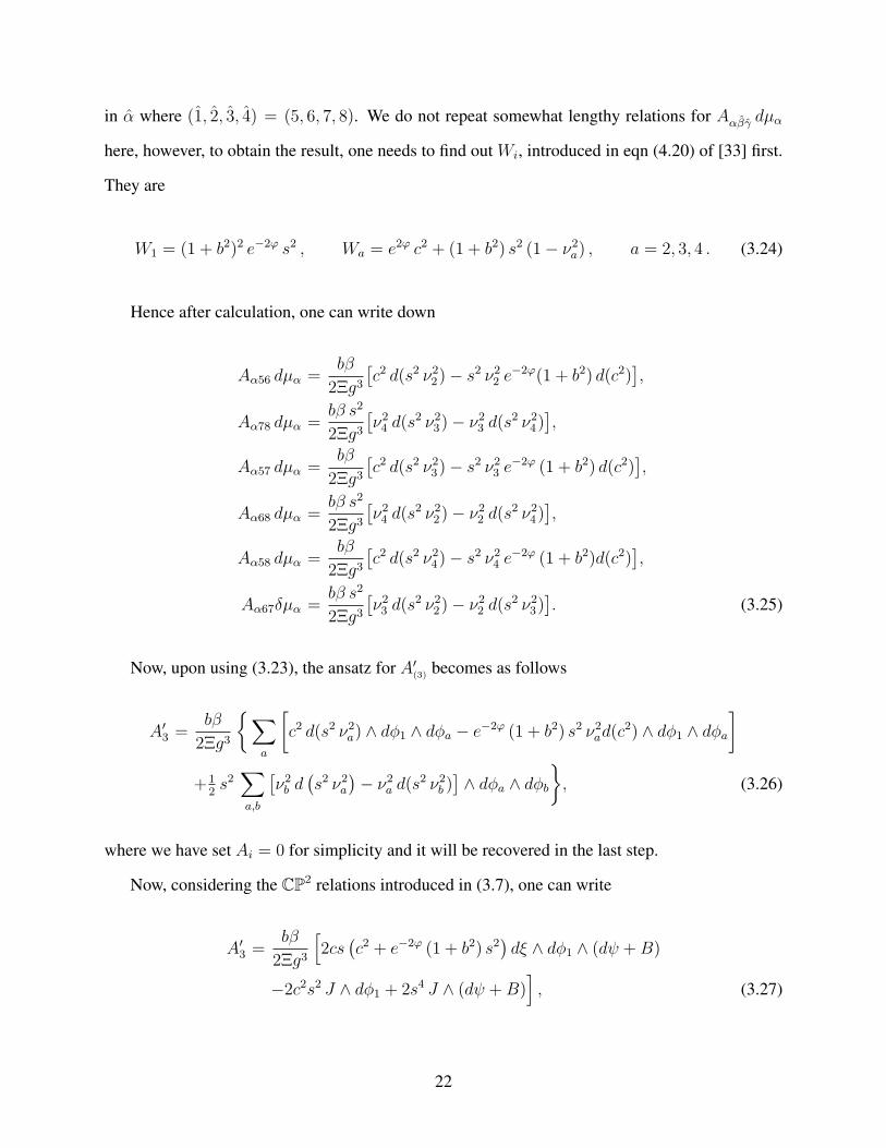
in α where (1, 2, 3, 4) = (5, 6, 7, 8). We do not repeat somewhat lengthy relations for Aαβγ dµα
here, however, to obtain the result, one needs to find out Wi, introduced in eqn (4.20) of [33] first.
They are
W1 = (1 + b2)2 e−2φ s2 , Wa = e2φ c2 + (1 + b2) s2 (1− ν2a) , a = 2, 3, 4 . (3.24)
Hence after calculation, one can write down
Aα56 dµα =bβ
2Ξg3[c2 d(s2 ν22)− s2 ν22 e
−2φ(1 + b2) d(c2)],
Aα78 dµα =bβ s2
2Ξg3[ν24 d(s
2 ν23)− ν23 d(s2 ν24)
],
Aα57 dµα =bβ
2Ξg3[c2 d(s2 ν23)− s2 ν23 e
−2φ (1 + b2) d(c2)],
Aα68 dµα =bβ s2
2Ξg3[ν24 d(s
2 ν22)− ν22 d(s2 ν24)
],
Aα58 dµα =bβ
2Ξg3[c2 d(s2 ν24)− s2 ν24 e
−2φ (1 + b2)d(c2)],
Aα67δµα =bβ s2
2Ξg3[ν23 d(s
2 ν22)− ν22 d(s2 ν23)
]. (3.25)
Now, upon using (3.23), the ansatz for A′(3) becomes as follows
A′3 =
bβ
2Ξg3
∑a
[c2 d(s2 ν2a) ∧ dϕ1 ∧ dϕa − e−2φ (1 + b2) s2 ν2ad(c
2) ∧ dϕ1 ∧ dϕa]
+12s2
∑a,b
[ν2b d
(s2 ν2a
)− ν2a d(s
2 ν2b )]∧ dϕa ∧ dϕb
, (3.26)
where we have set Ai = 0 for simplicity and it will be recovered in the last step.
Now, considering the CP2 relations introduced in (3.7), one can write
A′3 =
bβ
2Ξg3
[2cs
(c2 + e−2φ (1 + b2) s2
)dξ ∧ dϕ1 ∧ (dψ +B)
−2c2s2 J ∧ dϕ1 + 2s4 J ∧ (dψ +B)], (3.27)
22
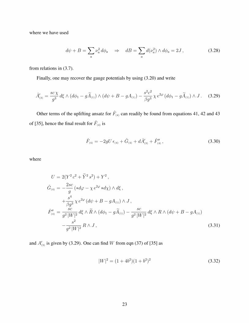
where we have used
dψ +B =∑a
ν2a dϕa ⇒ dB =∑a
d(ν2a) ∧ dϕa = 2J , (3.28)
from relations in (3.7).
Finally, one may recover the gauge potentials by using (3.20) and write
A′(3) =
sc χ
g3dξ ∧ (dϕ1 − gA(1)) ∧ (dψ +B − gA(1))−
s2c2
βg3χ e2φ (dϕ1 − gA(1)) ∧ J . (3.29)
Other terms of the uplifting ansatz for F(4) can readily be found from equations 41, 42 and 43
of [35], hence the final result for F(4) is
F(4) = −2gU ϵ(4) + G(4) + dA′(3) + F ′′
(4) , (3.30)
where
U = 2(Y 2 c2 + Y 2 s2) + Y 2 ,
G(4) = −2sc
g(∗dφ− χ e2φ ∗dχ) ∧ dξ ,
+s4
βg3χ e2φ (dψ +B − gA(1)) ∧ J ,
F ′′(4) =
sc
g2 |W |2dξ ∧ R ∧ (dϕ1 − gA(1))−
sc
g2 |W |2dξ ∧R ∧ (dψ +B − gA(1))
− s2
g2 |W |2R ∧ J , (3.31)
and A′(3) is given by (3.29). One can find W from eqn (37) of [35] as
|W |2 = (1 + 4b2)(1 + b2)2 (3.32)
23
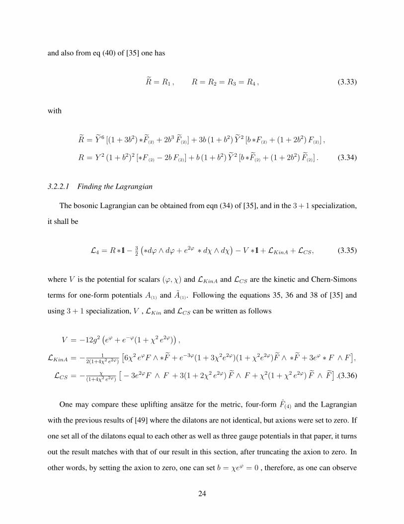
and also from eq (40) of [35] one has
R = R1 , R = R2 = R3 = R4 , (3.33)
with
R = Y 6 [(1 + 3b2) ∗F(2) + 2b3 F(2)] + 3b (1 + b2) Y 2 [b ∗F(2) + (1 + 2b2)F(2)] ,
R = Y 2 (1 + b2)2 [∗F (2) − 2b F(2)] + b (1 + b2) Y 2 [b ∗F(2) + (1 + 2b2) F(2)] . (3.34)
3.2.2.1 Finding the Lagrangian
The bosonic Lagrangian can be obtained from eqn (34) of [35], and in the 3+ 1 specialization,
it shall be
L4 = R ∗1l− 32
(∗dφ ∧ dφ+ e2φ ∗ dχ ∧ dχ
)− V ∗1l + LKinA + LCS, (3.35)
where V is the potential for scalars (φ, χ) and LKinA and LCS are the kinetic and Chern-Simons
terms for one-form potentials A(1) and A(1). Following the equations 35, 36 and 38 of [35] and
using 3 + 1 specialization, V , LKin and LCS can be written as follows
V = −12g2(eφ + e−φ(1 + χ2 e2φ)
),
LKinA = − 12(1+4χ2 e2φ)
[6χ2 eφF ∧ ∗F + e−3φ(1 + 3χ2e2φ)(1 + χ2e2φ)F ∧ ∗F + 3eφ ∗ F ∧ F
],
LCS = − χ(1+4χ2 e2φ)
[− 3e2φF ∧ F + 3(1 + 2χ2 e2φ) F ∧ F + χ2(1 + χ2 e2φ) F ∧ F
].(3.36)
One may compare these uplifting ansätze for the metric, four-form F(4) and the Lagrangian
with the previous results of [49] where the dilatons are not identical, but axions were set to zero. If
one set all of the dilatons equal to each other as well as three gauge potentials in that paper, it turns
out the result matches with that of our result in this section, after truncating the axion to zero. In
other words, by setting the axion to zero, one can set b = χeφ = 0 , therefore, as one can observe
24
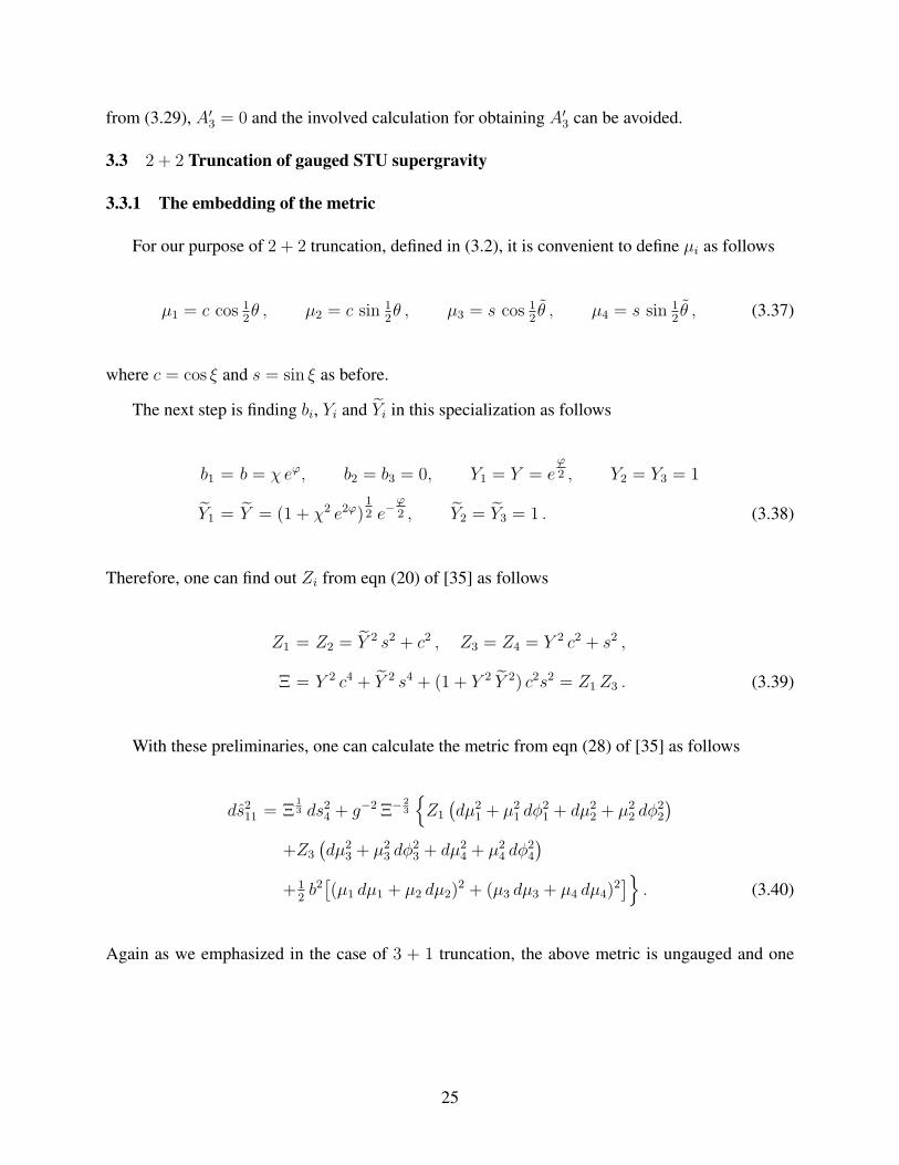
from (3.29), A′3 = 0 and the involved calculation for obtaining A′
3 can be avoided.
3.3 2 + 2 Truncation of gauged STU supergravity
3.3.1 The embedding of the metric
For our purpose of 2 + 2 truncation, defined in (3.2), it is convenient to define µi as follows
µ1 = c cos 12θ , µ2 = c sin 1
2θ , µ3 = s cos 1
2θ , µ4 = s sin 1
2θ , (3.37)
where c = cos ξ and s = sin ξ as before.
The next step is finding bi, Yi and Yi in this specialization as follows
b1 = b = χ eφ, b2 = b3 = 0, Y1 = Y = eφ2 , Y2 = Y3 = 1
Y1 = Y = (1 + χ2 e2φ)12 e−
φ2 , Y2 = Y3 = 1 . (3.38)
Therefore, one can find out Zi from eqn (20) of [35] as follows
Z1 = Z2 = Y 2 s2 + c2 , Z3 = Z4 = Y 2 c2 + s2 ,
Ξ = Y 2 c4 + Y 2 s4 + (1 + Y 2 Y 2) c2s2 = Z1 Z3 . (3.39)
With these preliminaries, one can calculate the metric from eqn (28) of [35] as follows
ds211 = Ξ13 ds24 + g−2 Ξ− 2
3
Z1
(dµ2
1 + µ21 dϕ
21 + dµ2
2 + µ22 dϕ
22
)+Z3
(dµ2
3 + µ23 dϕ
23 + dµ2
4 + µ24 dϕ
24
)+1
2b2[(µ1 dµ1 + µ2 dµ2)
2 + (µ3 dµ3 + µ4 dµ4)2]. (3.40)
Again as we emphasized in the case of 3 + 1 truncation, the above metric is ungauged and one
25
needs to follow (3.15) to gauge it. Using the definitions for µi in (3.37), one can write
ds211 = Ξ13 ds24 + g−2 Ξ− 2
3
Z1
[s2 dξ2 + 1
4c2dθ2 + c2
(cos2 1
2θ dϕ2
1 + sin2 12θ dϕ2
2
)]+Z3
[c2 dξ2 + 1
4s2dθ2 + s2
(cos2 1
2θ dϕ2
3 + sin2 12θ dϕ2
4
)]+ χ2 e2φ c2s2dξ2
. (3.41)
It is convenient to introduce the following relation for the four azimuthal angles
ϕ1 =12(ψ + ϕ) , ϕ2 =
12(ψ − ϕ) , ϕ3 =
12(ψ + ϕ) , ϕ4 =
12(ψ − ϕ) . (3.42)
Therefore, after some algebra, one can write
ds211 = Ξ13 ds24 + g−2 Ξ− 2
3
Ξ dξ2 + 1
4c2 (Y 2 s2 + c2)
(dθ2 + dψ2 + dϕ2 + 2dψ dϕ cos θ
)+1
4s2 (Y 2 c2 + s2)
(dθ2 + dψ2 + dϕ2 + 2dψ dϕ cos θ
). (3.43)
One needs to find out how the the gauge potentials incorporate in the Euler angles . Following
(3.15) and above definitions for azimuthal angles , one can readily find out
dϕ −→ dϕ , dψ −→ dψ − 2g A(1) ,
dϕ −→ dϕ , dψ −→ dψ − 2g A(1) . (3.44)
Having obtained these, one can easily complete the square in the metric ansatz (3.43), and after
considering the gauge potentials as it is stated in (3.44), one can write
ds211 = Ξ13 ds24 +
Ξ13
g2
dξ2 +
cos2 ξ
4Z3
[dθ2 + sin2 θ dϕ2 + (dψ + cos θ dϕ− 2gA(1))
2]
+sin2 ξ
4Z1
[dθ2 + sin2 θ dϕ2 + (dψ + cos θ dϕ− 2gA(1))
2]
, (3.45)
as it was presented in eqn (6.10) of [33].
One can compare the metric ansazt we have found, with the metric presented in eqn (1) of [34].
26
The latter result, studying the embedding of D = 4, N = 4 with SO(4) gauging supergravity in
eleven dimensions, is more general than what it was obtained here. However, one should find the
same result after considering an Abelian truncation of SO(4) gauging, i.e. U(1)2 gauging, with
A(1) and A(1) gauge potentials defined by (3.2). To make a connection with the eqn (1) of [34], one
needs to write down hi and hi 2, appeared in their metric, as follows
hi = σi − g Ai , hi = σi − g Ai , (3.46)
where σi are three left-invariant one-forms in S3 = SU(2). Note, since SO(4) = SU(2)×SU(2),
we have two copies of S3 here, where their corresponding gauge potentials are denoted by Ai and
Ai. One may explicitly write σi in terms of the Euler angles as follows
σ1 = cosψ dθ+sinψ sin θ dϕ , σ2 = − sinψ dθ+cosψ sin θ dϕ , σ3 = dψ+cos θ dϕ . (3.47)
With these preliminaries, one can find out∑
i h2i and
∑i h
2i in the metric ansatz in eqn (1)
of [34] as follows
∑i
h2i = dθ2 + sin2 θ dϕ2 + (dψ + cos θ dϕ− 2 gA(1))2
∑i
h2i = dθ2 + sin2 θ dϕ2 + (dψ + cos θ dϕ− 2 gA(1))2 , (3.48)
where as we have emphasized, just two gauge potentials A3 ≡ A(1) and A3 ≡ A(1) out of 6 gauge
potentials of SO(4) are kept.
Finally, Setting Ξ = ∆2, and rescaling g = 1√2gRef. [34], one can retrieve eqn (1) of [34] from
the metric presented in (3.45).
One may set χ = 0 to find a further truncation which was studied in [49] for the first time.
2In chapter 4, the combination of the left-invariant one-forms and the gauge potentials will be denoted by νi.
27
Hence, with this assumption, one has
Y = e12φ , Y = e−
12φ , Ξ ≡ ∆2 = e−φ
(eφ c2 + s2
)2, (3.49)
and it can be observed the resulting ansatz is the same as that of eqn (3.1) of [49] and also eqn (44)
of [34].
3.3.2 The embedding of the four-form
Full ansatz of the embedding of the four-form of gauged STU supergravity in eleven dimen-
sions is given in section 4 and 5 of [33]. In this part, we find out the uplift of the four-form in 2+2
truncation of gauged STU supergravity and we will show it is in full agreement with the result
derived in [34].
One can follow the same route as it was taken in the 3 + 1 truncation, and use the ansatz in
(3.22). Let us calculate A′(3) contribution in four-form field strength first. To do so, one needs to
find out Wi in eqn (4.20) of [33] as follows
W1 = c2 sin2 12θ + s2Y 2 , W2 = c2 cos2 1
2θ + s2Y 2 ,
W3 = s2 sin2 12θ + c2Y 2 , W4 = s2 cos2 1
2θ + c2Y 2 . (3.50)
The next step is finding Aαβγ dµα from eqn (4.19) of [33]. Here we have introduced the hat
notation in α where (1, 2, 3, 4) = (5, 6, 7, 8). Since b2 = b3 = 0, it leads to a considerable
simplification. The results become
Aα56 dµα =b
2Ξ g3
[µ21W2 d(µ
22)− µ2
2W1 d(µ21)− µ2
1 µ22 d(α2 + α3)
],
Aα78 dµα =b
2Ξ g3
[µ24W3 d(µ
23)− µ2
3W4 d(µ24) + µ2
3 µ24 d(α2 − α3)
],
Aα57 dµα = Aα68 dµα = Aα58 dµα = Aα67 dµα = 0 , (3.51)
28
where
α1 = µ21 + µ2
2 α2 = µ21 + µ2
3 , α3 = µ21 + µ2
4 . (3.52)
Now, one needs to make use of the reparametrizations introduced in (3.37) and the result is
Aα56 dµα = b c4
4Ξ g3(s2 Y 2 + c2) sin θ dθ , Aα78 dµα = −b s4
4Ξ g3(s2 + Y 2 c2) sin θ dθ . (3.53)
The next step is using the expression (5.5) in [33] for finding A′(3), which we already presented
in (3.23). According to eqn (3.51), just two terms contribute in (3.23) relation, hence one can write
down
A′(3) =
χ eφ
4Ξ g3
(c4 sin θ (c2 + s2 Y 2) dθ ∧ (dϕ1 − g A(1)) ∧ (dϕ2 − g A(1))
−s4 sin θ (s2 + c2 Y 2) dθ ∧ (dϕ3 − g A(1)) ∧ (dϕ4 − g A(1))). (3.54)
Now, making use of (3.42), one can obtain
A′(3) =
χ eφ
8 g3
( c4
s2 + c2 Y 2sin θ dθ ∧ dϕ ∧ (dψ − 2g A(1))
− s4
c2 + s2 Y 2sin θ dθ ∧ dϕ ∧ (dψ − 2g A(1))
). (3.55)
To relate the above result to that of [34] in eqn (7), one has to find out
ϵ(3) ≡ 16εijk h
i ∧ hj ∧ hk = h1 ∧ h2 ∧ h3 = σ1 ∧ σ2 ∧ (σ3 − 2g A(1))
= sin θ dθ ∧ dϕ ∧ (dψ − 2g A(1)) , (3.56)
where we have used (3.47). One can obtain the similar result for ϵ(3) and hence, can verify
A′(3) = f ϵ(3) + f ϵ(3) , (3.57)
29
where
f =χ eφ c4
8g3 (s2 + c2 Y 2), f = − χ eφ s4
8g3 (c2 + s2 Y 2). (3.58)
It turns out this is the same result as eqn (8) of [34] with the above mentioned rescaling for the
coupling constant g, i.e. g = 1√2gRef. [34].
To obtain the full ansatz for the four-form field strength, one needs to find out other parts of it.
To do so, one may calculate F ′′(4), presented in eq (43) of [35] as follows
F ′′(4) = − 1
2g2|W |−2
∑i
dµ2i ∧ (dϕi − g Ai(1)) ∧Ri . (3.59)
Here Ri are two-forms introduced in eqn (40) of [35] and according to 2 + 2 specialization, they
read
R1 = R2 = Y 2 (1 + b2) (∗F(2) + bF(2)) , R3 = R4 = Y 2 (1 + b2) (∗F(2) − bF(2)) , (3.60)
where F(2) = dA(1) and F(2) = dA(1). Also, as it can be obtained easily from eqn (37) of [35],
W = 1 + b2. Now, making use of the following relations
dϕ1 − g A = 12(dψ + dϕ− 2g A) = 1
2h3 + sin2 1
2θ dϕ ,
dϕ2 − g A = 12(dψ − dϕ− 2g A) = 1
2h3 − cos2 1
2θ dϕ , (3.61)
one can write down the following result for F ′′(4)
F ′′(4) =
1
2g2 (1 + b2)
[e−φ (cs dξ ∧ h3 + 1
2c2 h1 ∧ h2) ∧ (∗F(2) + bF(2))
+eφ (−cs dξ ∧ h3 + 12s2 h1 ∧ h2) ∧ (∗F(2) − bF(2))
]. (3.62)
Again with the rescling of the coupling constant , one can obtain the same result as eqn (10) of [34],
after applying an appropriate truncations.
The only remaining term for finding the complete uplift ansazt for four-form is G(4) which can
30
be readily obtained by using eqn (5.8) of [33]. Hence the full ansatz reads
F(4) = −2g U ϵ(4) + dA′(3) + F ′′
(4) +cs
g(− ∗ dφ+ e2φ χ ∗ dχ) ∧ dξ , (3.63)
where U = c2Y 2 + s2Y 2 + 2 and A′(3) and F ′′
(4) are given by (3.57) and (3.62) respectively. Again,
one may check the above ansatz is consistent with the truncated result in [34] after applying the
rescaling in the coupling constant.
3.3.3 Finding the bosonic Lagrangian
The bosonic Lagrangian, as we mentioned in 3 + 1 case, can be derived from eqn (34) of [35].
It reads
L4 = R ∗1l− 12
3∑i=1
(∗dφi ∧ dφi + e2φi ∗dχi ∧ dχi)− V ∗1l + LKin + LCS . (3.64)
Note that since b2 = b3 = 0, this leads to a great deal of simplicity in calculation. One may readily
calculate V , LKin and LCS from eqn (35) , eqn (36) and eqn (38) of [35] respectively and the result
is
L = R ∗1l− 12∗dφ ∧ dφ− 1
2e2φ ∗dχ ∧ dχ− V ∗1l
−Y −2 ∗F (2) ∧ F(2) − Y −2 ∗F (2) ∧ F(2)
−χF(2) ∧ F(2) + χY 2 Y −2 F(2) ∧ F2 , (3.65)
where
V = −4g2 (Y 2 + Y 2 + 4) . (3.66)
Therefore, we could be able to recover all results which previously presented in [34] for case
of 2 + 2 truncation of gauged STU supergravity.
31
4. ON THE PAULI REDUCTION OF MINIMAL SUPERGRAVITY IN FIVE DIMENSIONS
4.1 Introduction
In this chapter, we address the possibility of the consistent Pauli S2 Reduction of minimal
supergravity in five dimensions. The main motivation for this investigation, is the resemblance
between the bosonic Lagrangian of this theory and that of eleven-dimensional supergravity, which
can be observed from the following expressions
L5 = R∗1l− 12∗F(2) ∧ F(2) − 1
3√3F(2) ∧ F(2) ∧ A(1) ,
L11 = R∗1l− 12∗F(4) ∧ F(4) − 1
6F(4) ∧ F(4) ∧ A(3) , (4.1)
where F(2) = dA(1) and F(4) = dA(3). Since there are S7, S4 and S5 consistent Pauli reductions
of the latter theory, one wonders about the existence of S2 or S3 consistent Pauli reductions of the
former one.
One may study this problem by writing a trial ansatz, and then considering the five-dimensional
equations of motion, if the internal manifold coordinates (S2 components in this case) remarkably
conspire and cancel out in these equations, one can claim the consistent ansatz has been found. The
important point is, this ansatz should include the gauge bosons with gauge group of the isometry
of the internal manifold (in this case, three gauge bosons with SU(2) gauging). Using this method,
the construction of the ansatz was not successful. Therefore, we investigated another method,
which is a more systematic one, and can be used to study the other cases as well.
This method, originally presented in [7], was named the “Hopf fibration technique” in [45]. The
idea is starting from a higher dimensional theory and performing a (necessary consistent) DeWitt
reduction on a group manifold G, then again from the initial theory, one can perform another
DeWitt reduction on a group manifold H , where the latter group is a sub-group of the former one.
Now, viewing the group manifoldG as anH Hopf fibration overG/H , it is guaranteed by a group-
theoretical argument that the coset reduction G/H is indeed consistent. In our case, the higher
32
dimensional theory is minimal six-dimensional supergravity. We implement a consistent DeWitt
SU(2) reduction on this theory and find a three-dimensional space-time. In addition to this, we
perform a consistent Kaluza-Klein S1 reduction to obtain minimal five-dimensional supergravity
coupled to a vector multiplet. Now, writing the group manifold SU(2) as a U(1) Hopf fibration
over SU(2)/U(1) = S2 coset space, one can obtain a consistent Pauli S2 reduction from the five-
dimensional theory to the three-dimensional one. However, to accomplish the task of finding the S2
reduction of minimal five-dimensional supergravity, one needs to perform a consistent truncation
in five dimensions. But, as we will clarify later, this truncation gives rise to the vanishing of the
field strengths, and hence it implies the impossibility of the S2 reduction of this theory.
The rest of this chapter organizes as follows. In section 4.2 , we will obtain an S1 reduction
of minimal six-dimensional supergravity, and find a relation, due to the self-duality of three-form
field strength in six dimensions, between two- and three- form field strengths in five dimensions.
In section 4.3, we will present an S3 = SU(2) DeWitt reduction from six-dimensional minimal
supergravity down to a three-dimensional space-time. Also, we consider this S3 as a Hopf fibration
of U(1) over an S2, and by this means, write down the SU(2) DeWitt ansätze in a Hopf fibration
fashion. Hence by comparing these ansätze with those of the circle reduction in section 4.2.2, one
can find finally the ansätze for S2 reduction of minimal supergravity coupled to a vector multiplet.
However, as we will show in section 4.4, the truncation we have found for obtaining pure minimal
supergravity in five dimensions is not compatible with our ansätze, meaning that, one cannot find
a consistent Pauli S2 reduction of minimal D = 5 supergravity using the Hopf fibration technique.
4.2 S1 reduction of minimal D = 6 supergravity
The field content of the bosonic sector of minimal supergravity in six dimensions consists of a
metric gMN and a two-form potential B(2) whose field strength is a self-dual field, i.e. H(3) =
dB(2) = ∗H(3). Our convention is to insert a hat on the six-dimensional and a bar on five-
dimensional fields to avoid any ambiguity. In any 4n + 2 dimensions, self duality of the field
33
strength, ∗H(2n+1) = H(2n+1) yields to
∗H(2n+1) ∧H(2n+1) = H(2n+1) ∧H(2n+1) = −H(2n+1) ∧H(2n+1) = 0 . (4.2)
Hence, it is not possible to write down a Lagrangian for this theory and one should state equations
of motion instead. However, minimal supergravity in six dimensions can be derived from the
following six-dimensional bosonic string Lagrangian with an appropriate truncation
L = R ∗1l− 12∗dϕ ∧ dϕ− 1
4ea ϕ ∗H(3) ∧ H(3) , (4.3)
where H(3) = dB(2), and a2 = 8D−2
= 2. Here, ∗, ∗ and ∗ denote the Hodge dual of forms in 6, 5
and 3 dimensions respectively. Therefore, the equations of motion read
RMN = − eaϕ
12(D − 2)H2 gMN + 1
2∂M ϕ ∂N ϕ+ eaϕ
8H2MN ,
ϕ = a24eaϕ H2, (4.4)
d(eaϕ∗H(3)
)= 0,
where H2 = HMNP HMNP , and H2
MN = HMPQ HNPQ. Now, upon imposing the self duality
condition on three-form field strength, one obtains H2 = 0. Then to have a consistent truncation,
due to the second equation of (4.4), the scalar field should be set to zero. Therefore, the truncated
theory, which is the bosonic sector of minimal supergravity in six dimensions, has the following
equations of motion
RMN = 18H2MN , d∗H(3) = 0, ∗H(3) = H(3). (4.5)
34
4.2.1 A Kaluza-Klein circle reduction to 5D
According to the standard Kaluza-Klein S1 reduction presented in chapter 2, one can write
ds26 = e2αϕ ds25 + e2βϕ (g−1 dτ +A(1))2 , (4.6)
H(3) = dB(2) , B(2) = B(2) +B(1) ∧ g−1 dτ , H(3) = H(3) + H(2) ∧ (g−1 dτ +A(1)) ,
where we choose α2 = 124
and β = −3α to find a canonically normalized kinetic term for the
“breathing mode" ϕ in five-dimensional bosonic Lagrangian. Here z = g−1 τ has the dimensions
of length, while τ is a dimensionless coordinate. As usual, the higher dimensional relations above
yield the following relations in five dimensions
H(3) = dB(2) − dB(1) ∧ A(1) , H(2) = dB(1) . (4.7)
One can find the six-dimensional dual of the field strength as follows
∗H(3) = ∗H(3) + ∗(H(2) ∧ (dz +A(1))
)= (−1)3×1 e−αϕ eβϕ ∗H(3) ∧ (dz +A(1))
+(−1)2×0 eαϕ e−βϕ ∗H(2) = −e−4αϕ ∗H(3) ∧ (dz +A(1)) + e4αϕ ∗H(2) . (4.8)
Now, the self duality condition implies
H(3) = e4αϕ ∗H(2) , (4.9)
in five dimensions. Therefore, the six-dimensional three-form field strength shall be
H(3) = e4αϕ ∗H(2) +H(2) ∧ (dz +A(1)) . (4.10)
35
4.2.2 Finding the bosonic Lagrangian in 5D
The six-dimensional Einstein equation, writing in the flat indices, has a simple form
RAB = 18HA
CDHBCD . (4.11)
Now one needs to find the components of H2AB = HA
CDHBCD in five dimensions. To do
so, from (4.7) one can obtain the following relations for the flat components of the five- and six-
dimensional field strengths as usual
Habc = e−3αϕHabc , Hab6 = eαϕHab , (4.12)
where the above five-dimensional field strengths are clearly a three-form and a two-form fields
respectively, and for simplicity we refrain to insert the subscripts when there is no ambiguity.
Recalling the self duality relation (4.9), one has the following result for the components of H(3)
and H(2)
Habc =12e4αϕ ϵabc
deHde . (4.13)
Therefore, using the above relation, one can obtain the following expressions for the components
of H2AB
H2ab = Hacd Hb
cd + 2Hac6 Hbc6 = e−6αϕHacdHb
cd + 2eαϕHacHbc
= 14e2αϕ ϵacdef H
df ϵbcdghHgh + 2eαϕHacHb
c = e2αϕ (−ηabHcdHcd + 4HacHb
c) ,
H2a6 = Habc H6
bc = e−2αϕHabcHbc = 1
2e2αϕ ϵabcdeH
bcHde ,
H266 = H6ab H6
ab = e2αϕHabHab . (4.14)
Using the expressions for higher dimensional Ricci components in (2.13) of chapter 2, one has
36
the following five-dimensional relations for the higher dimensional Einsteins equation in (4.11)
Rab = e−2αϕ(Rab − 1
2∂aϕ ∂bϕ− 1
2e−8αϕF2
ab − α ηabϕ)
= 18e2αϕ (−ηabHcdH
cd + 4HacHbc) ,
Raz = Rzb =12e2 αϕ∇b
(e−8αϕFab
)= 1
16e2αϕ ϵabcdeH
bcHde , (4.15)
Rzz = e−2αϕ(3αϕ+ 1
4e−8αϕF2
)= 1
8e2αϕHabH
ab .
In differential geometry, there is an operator which is the adjoint of the exterior derivative (
sometimes called the interior derivative) which can be written as follows
(δ ω(p))µ1···µp−1 ≡ (−1)np+t (∗d ∗ ω(p))µ1···µp−1 = −∇µ ωµµ1···µp−1 , (4.16)
where ω(p) is a p-form and n and t are the number of space-time and time-like dimensions respec-
tively. Having used this relation, one can write the second equation of (4.15) in the form language
as follows
d(e−8αϕ ∗F(2)) = −12H(2) ∧H(2) . (4.17)
Having obtained the above equation, now it is not hard to find a five-dimensional Lagrangian
which yields the three equations in (4.15) as an Einstein, a one-form gauge potential A(1) and a
scalar equations of motion. From the right hand side of (4.17), one needs to include the term
−12H(2) ∧ H(2) ∧ A(1) in the Lagrangian, while the pre-factors of the kinetic terms may be found
from the third equation in (4.15), i.e. the scalar equation of motion. The five-dimensional bosonic
Lagrangian shall be written as
L5 = R ∗1l− 12∗dϕ∧ dϕ− 1
2e−8αϕ ∗F(2) ∧F(2) − 1
2e4αϕ ∗H(2) ∧H(2) − 1
2H(2) ∧H(2) ∧A(1) . (4.18)
The first equation of (4.15), upon using the scalar equation of motion, gives rise to the Einstein
equation derived from the above Lagrangian. However, the equation for B(1) , the gauge potential
37
whose field strength isH(2) = dB(1), did not appear in (4.15), but it can be derived from the Bianchi
identity, i.e. dH(3) = 0. Namely, using (4.10), one has
dH(3) = d(e4αϕ ∗H(2)
)+H(2) ∧ F(2) = 0. (4.19)
This is exactly the equation for the gauge potential B(1) derived from the above Lagrangian.
4.2.3 Truncations to minimal supergravity in 5D
The Lagrangian we found in (4.18) is five dimensional minimal supergravity coupled to one
vector multiplet. One needs to perform the following truncation to obtain minimal supergravity in
five dimensions
ϕ = 0 , H(2) =√2F(2) . (4.20)
The factor of√2 is crucial here, since, to satisfy the third equation of (4.15), upon truncation of the
scalar field to zero, the presence of this factor guarantees the source term for the truncated scalar
field is also vanishing.
To have a canonical normalization for the kinetic term of the field strength, one may use the
following field redefinition
A(1) =√3A(1) . (4.21)
Hence, the bosonic Lagrangian shall be that of pure minimal supergravity in five dimensions
L5 = R ∗1l− 12∗F(2) ∧ F(2) − 1
3√3F(2) ∧ F(2) ∧ A(1) . (4.22)
4.3 SU(2) DeWitt reduction from D = 6 to D = 3
In this section, we consider a consistent SU(2) DeWitt reduction of minimal supergravity in six
dimensions down to a three-dimensional theory. This construction was already presented in [44]
and we shall review it here.
It is convenient to present the general DeWitt reduction ansatz of the Einstein-Hilbert action
38
in D = n + q dimensions reduced on a q-dimensional group manifold. The metric ansatz, stated
in [7], and it is
ds2(n+q) = e2αφ ds2(n) + g−2e2βφ Tij νi νj, (4.23)
where one-forms νi
νi = σi − gAi , (4.24)
are written in terms of the left-invariant one-forms σi in the group manifold. The unimodular ma-
trix Tij parameterizes the remaining scalar fields of the n-dimensional theory. The scalar field φ is
a “breathing mode" and constants (α, β) shall be determined by demanding the lower dimensional
Lagrangian has no scalar pre-factor in the Einstein-Hilbert term and the scalar has a canonically
normalized kinetic term. Hence the constants are
α = −√
q
2(n− 2)(n+ q − 2), β = −α (n− 2)
q. (4.25)
We investigate the case of G = SU(2) in the following.
4.3.1 The ansätze for an SU(2) group manifold reduction
The reduction ansätze for the metric and the self-dual three-form are the following
ds26 = e2αφds23 + g−2 e2βφ Tij νi νj , (4.26)
H(3) = mg−3Ω(3) +me4αφ ϵ(3) +12g−2 εijk B
i ∧ νj ∧ νk − g−1e4αφ3 Tij ∗Bi ∧ νj , (4.27)
where the constants α and β can be found from (4.25) by setting (n, q) = (3, 3) and they are given
by α2 = 38
and β = −α3
. One-forms νi are given by (4.24) as νi = σi− gAi and three left invariant
one-form σi are expressed as the following expression in terms of the Euler angles (ψ, θ, τ)
σ1 = cosψ dθ+sinψ sin θ dτ , σ2 = − sinψ dθ+cosψ sin θ dτ , σ3 = dψ+cos θ dτ , (4.28)
39
and they satisfy the following relation
dσi = −12εijk σj ∧ σk . (4.29)
The three-form Ω(3) is defined by
Ω(3) ≡ ν1 ∧ ν2 ∧ ν3 , (4.30)
where ϵ(3) is the volume form of the three-dimensional space-time, andBi denotes an SU(2) triplet
of one-form fields.
One can define the covariant derivative and the field strength of the SU(2) gauge potentials Ai
as usual
Dνi ≡ dνi + g εijk Aj ∧ νk F i = dAi + 1
2g εijk A
j ∧ Ak . (4.31)
Then, one can find an expression for Dνi as follows
Dνi ≡ dνi + gεijk Aj ∧ νk = dσi − g dAi + gεijk A
j ∧ νk = −12εijk σj ∧ σk (4.32)
−g dAi + gεijk Aj ∧ νk = −1
2εijk (νj + gAj) ∧ (νk + gAk)− g dAi + gεijk A
j ∧ νk
= −12εijk νj ∧ νk − 1
2gεijk νj ∧ Ak − 1
2gεijk Aj ∧ νk − 1
2g2 εijk Aj ∧ Ak − g dAi
+g εijk Aj ∧ νk = −g dAi − 1
2g2 εijk Aj ∧ Ak − 1
2εijk νj ∧ νk = −1
2εijk νj ∧ νk − g F i .
Using (4.27) and the Bianchi identity dH(3) = 0 one has
dH(3) = DH(3) = mg−3 dΩ(3) +12g−2εijkDB
i ∧ νj ∧ νk − g−2εijk Bi ∧Dνj ∧ νk
−g−1 43α e
4αφ3 Tij dφ ∧ ∗Bi ∧ νj − g−1 e
4αφ3 DTij ∧ ∗Bi ∧ νj
−g−1 e4αφ3 Tij ∧ ∗Bi ∧Dνj − g−1 e
4αφ3 Tij ∧D ∗Bi ∧ νj = 0 . (4.33)
We are interested in terms involving νj ∧ νk, and since they are independent of those terms
40
which involving νi, then the former terms should be vanishing according to the above equation.
Also using (4.30), the following expression for dΩ(3) can be written
dΩ(3) =36εijkDν
i ∧ νj ∧ νk = −12g εijk F
i ∧ νj ∧ νk . (4.34)
Then, according to the above argument about the vanishing of terms involving νj∧νk in (4.33),
one can conclude
εijk νj ∧ νk ∧
(− 1
2mg−2 F i + 1
2g−2DBi + 1
2g−1e
4αφ3 Tiℓ ∗Bℓ
)= 0 . (4.35)
In other words
DBi −mF i + ge43αφ Tij ∗Bj = 0 , (4.36)
where DBi = dBi + g εijk Aj ∧Bk.
Upon plugging in the ansätze (4.26) and (4.27) into the six dimensional equations of motion
(4.5), one can find the three-dimensional equations of motion and it can be derived from a bosonic
Lagrangian presented in [44].
4.3.2 SU(2) as a Hopf fibration
So far, we have obtained a circle reduction of minimal supergravity in six dimensions and
also an SU(2) reduction of that theory. Now, one can re-interpret the latter reduction as a U(1)
Hopf fibration of the circle reduction over S2. Hence, one can find a consistent S2 reduction of
five-dimensional theory. The crucial point here is, one needs to re-write elements of the SU(2)
reduction in the Hopf fibration manner.
To describe the S2 reduction, one may introduce three Cartesian coordinates µi, where µi µi =
1, to describe the unit two-sphere in R3. One may use the following re-parametrization in terms of
the Euler angles (θ, ψ)
µ1 = sinψ sin θ , µ2 = cosψ sin θ , µ3 = cos θ . (4.37)
41
Now, one needs to find relations between elements of the SU(2) reduction and these three
parameters. The starting point is the following expression between the three parametrization coor-
dinates and the three left-invariant one-forms
dµi = εijk µj σk , (4.38)
where σi are defined in (4.28). One can easily verify the above relation by a direct calculation.
Now, considering the gauge fields, the above relation yields to the following
Dµi = εijk µj νk , (4.39)
where the covariant derivative is defined as Dµi ≡ dµi + g εijk Aj µk . Now, having obtained that,
let us find the following combination
εijk µj Dνk = εijk µ
j εkmn µm νn = µj (µi νj − µj νi) = µi (µj νj)− νi . (4.40)
Therefore one can write
νi = σi − g Ai = −εijk µj Dµk + µi σ ,
σ ≡ µi νi = dτ + cos θ dψ − g µiAi . (4.41)
At this stage, it is useful to introduce some relations which will be needed to perform the
calculations. First, we present two well-known relations in linear algebra about the determinant
and the inverse of a general n× n matrix
detA = εi1i2···in A1i1 A2i2 · · ·Anin = 1n!εi1i2···in εj1j2 · · · jnAi1j1 Ai2j2 · · ·Ainjn ,
A−1ij = 1
(n−1)!1
detAεi i2···in εj j2···jn Aj2i2 · · ·Ajnin , (4.42)
where the second relation above can be derived from the first one, by multiplyingA−1ij in both sides
42
of the first relation and using a useful identity named Schouten’s trick. The latter is as follows
ε[i1i2···in Mi] = 0 ⇒ εi1i2···in Mi = εi i2···in Mi1 + εi1 i···in Mi2 + · · · εi1i2···iMin . (4.43)
Since the anti-symmetrization of n+1 components where each of them runs over n value, is always
vanishing, hence the result is obvious, but, in spite of its simplicity, it is a very powerful tool and
we have used it frequently in our calculations.
Let us employ (4.42) to find a useful lemma
εijk AjmAkn = detA εℓmnA−1ℓi , (4.44)
where it can be proved as follows
εℓmnA−1ℓi = 1
21
detAεℓmn εℓpq εijk AjpAkq =
12
1detA
εijk (AjmAkn − AjnAkm)
= 1detA
εijk AjmAkn . (4.45)
Therefore, for the case of Aij = Tij , one has
εijk Tjm Tkn = T−1iℓ εℓmn , (4.46)
where we have used the fact that Tij is uni-modular and symmetric.
To obtain the Hopf fibration result for SU(2) reduction metric ansatz in (4.26), one needs to
find a relation for Tij νi νj . Using (4.41) one can calculate
Tij νi νj = Tij (−εimn µmDµn + µi σ) (−εjpq µpDµq + µj σ) = Tij εimn εjpq µ
m µpDµnDµq
−2Tij εikℓ µk µj Dµℓ σ + ∆σ2 = ∆
(σ − ∆−1 Tij εikℓ µ
k µj Dµℓ)2
+M , (4.47)
where ∆ = Tij µiµj . We try to complete the square and M denotes the remaining terms to be
found later. Our motivation to complete the square term is to find a (dτ+gA)2 term which appears
43
in the S1 reduction. Taking into account νi is a dimensionless quantity, one may have the following
relation
σ − ∆−1 Tij εikℓ µk µj Dµℓ = dτ + gA , (4.48)
and considering σ from (4.41), one can write the following relation for the Kaluza-Klein vector
gauge potential
A = g−1 cos θ dψ − µiAi − g−1 ∆−1 Tij εikℓ µjµkDµℓ . (4.49)
Now, one needs to find M . From (4.47), one can write the following expression for M
M = ∆−1(∆ Tij εimn εjpq µ
m µpDµnDµq −(Tij εikℓ µ
k µj Dµℓ)2)
. (4.50)
Writing ∆ = Trs µrµs, the first term of the right hand side of the above relation shall be written
as
∆ Tij εimn εjpq µm µpDµnDµq = Trs µ
rµs Tij εimn εjpq µm µpDµnDµq
= Trs Tij (εrpq µj + εjrq µ
p + εjpr µq) εimn µ
sµmµpDµnDµq
= (Trs εrpq µsµpDµq)(Tij εimn µ
jµmDµn)
+εisp T−1pq εimn µ
sµmDµnDµq
=(Tij εikℓ µ
k µj Dµℓ)2
+ T−1ij DµiDµj , (4.51)
where we have use the following relations
µr εjpq = εrpq µj + εjrq µ
p + εjpr µq ,
εjrq Trs Tij = εisp T−1pq , µiµi = 1 , µiDµi = 1
2D(µiµi) = 0 . (4.52)
Now, upon using (4.50) and (4.51) then M has a simple form
M = ∆−1 T−1ij DµiDµj . (4.53)
44
Finally, the metric ansatz (4.26) can be written in the Hopf fibration form
ds26 = e2αφ ds23 + g−2 e2βφ ∆−1 T−1ij DµiDµj + g−2 e2βφ ∆ (dτ + gA)2 , (4.54)
where the Kaluza-Klein vector potential A has defined in (4.49).
The next step is finding a Hopf fibration expression for the three-form field strength H(3).
Before calculating it, let us introduce some useful relations
νi = µi (dτ + gA)− ∆−1 Tjk εijℓ µkDµℓ , (4.55)
12εijk ν
j ∧ νk = (dτ + gA) ∧Dµi + ∆−1 Tij µj ω(2) , (4.56)
Ω(3) =16εijkν
i ∧ νj ∧ νk = (dτ + gA) ∧ ω(2) , (4.57)
where
ω(2) =12εijk µ
iDµj ∧ Dµk . (4.58)
To prove (4.55), one can start from (4.41) to write
νi = −∆−1 Tmn µmµn εijk µ
j Dµk + µi(dτ + gA+ ∆−1 Tij εikℓ µ
jµkDµℓ)
= −∆−1(Tmn (εmjk µ
i + εimk µj + εijm µ
k)µnµj Dµk − Tij εikℓ µiµjµkDµℓ
)+µi (dτ + gA) = µi (dτ + gA)− ∆−1 Tjk εijℓ µ
kDµℓ , (4.59)
where we have used the Schouten’s identity in the second line above and using the following
expression for σ
σ = dτ + cos θ dψ − g µiAi = dτ + gA+ ∆−1 Tij εikℓ µjµkDµℓ . (4.60)
45

To prove (4.56) , one can use (4.55)
12εijk ν
j ∧ νk = 12εijk
(µj (dτ + gA)− ∆−1 εjmℓ Tmn µ
nDµℓ)
×(µk (dτ + gA)− ∆−1 εkpq Tpr µ
rDµq)= −∆−1 εijk εjmℓ Tmn µ
nµkDµℓ
∧ (dτ + gA) + 12∆−2 εijk εjmℓ Tmn µ
n εkpq Tpr µr εℓqs µ
s ω(2) (4.61)
= −∆−1 (TknDµi − TinDµ
k)µnµk ∧ (dτ + gA)
+12∆−2 (Tir εℓjs − Tjr εℓis) εjmℓ Tmn µ
nµrµs ω(2) = (dτ + gA) ∧ Dµi
+∆−1 Tij µj ω(2) − 1
2∆−2 (Tir Tsn − Tsr Tin)µ
nµrµs ω(2)
= (dτ + gA) ∧Dµi + ∆−1 Tij µj ω(2) ,
where we have used
Dµi ∧Dµj = εijk µk ω(2) . (4.62)
Its proof is the following
Dµi ∧Dµj = 12εijk εkpqDµ
p ∧Dµq = 12εijk εkpqDµ
p ∧Dµq µm µm
= 12εijk (εmpq µ
k + εkmq µp + εkpm µ
q)Dµp ∧Dµq µm
= 12εijk εmpq µ
mDµp ∧Dµq µk = εijk µk ∧ ω(2) . (4.63)
Note that from (4.56) by multiplying µi in both sides, one obtains
12εijk µ
i νj ∧ νk = ω(2) . (4.64)
There is also another expression for ω(2). Multiplying both sides of the first relation of (4.41)
by Dµi, one can easily find
ω(2) =12Dµi ∧ νi . (4.65)
46
Making use of (4.65) , (4.32) and (4.41), one may calculate
ω(2) = −12εijk µ
i νj ∧ νk + 2ω(2) = µi (Dνi + gF i) +Dµi ∧ νi = D(µiνi) + gµiF i
= dσ + gµiF i = sin θ dψ ∧ dθ − g d(µiAi) + g µiF i . (4.66)
Finally (4.57) can be proved as follows
(dτ + gA) ∧ ω(2) = µmνm ∧ ω(2) =12εijk µ
i µmνm ∧ νj ∧ νk = 12εijk µ
i µm εmjk Ω(3) = Ω(3) ,
where we multiply µi in both sides of (4.55) and also employ the relation
Dµi ∧Dµj ∧Dµk = εijk ω(3) ⇒ ω(3) =16εijkDµ
i ∧Dµj ∧Dµk = 16µmµm εijkDµ
i ∧Dµj ∧Dµk
= 16µm(εmjk µ
i + εimk µj + εijm µ
k)Dµi ∧Dµj ∧Dµk = 0 . (4.67)
After these preliminaries, now we may find the Hopf fibration form of the self-dual field
strength H(3) given by (4.27)
H(3) = mg−3 dτ + gA) ∧ ω(2) +me4αφ ϵ(3) + g−2Bi ∧((dτ + gA) ∧Dµi + ∆−1 Tij µ
j ω(2)
)−g−1e
4αφ3 Tij ∗Bj ∧
(µi (dτ + gA)− ∆−1 εimℓ Tmk µ
kDµℓ)
(4.68)
= d(τ + gA) ∧[mg−3 ω(2) − g−2Bi ∧Dµi − g−1 e
43αφ Tij µ
i ∗Bj]
+me4αφ ϵ(3) + g−2 ∆−1 Tij µiBj ∧ ω(2) + g−1e
43αφ ∆−1 εjkm µ
ℓ Tij Tkℓ ∗Bi ∧Dµm .
Now we have all ingredients of re-interpreting the DeWitt SU(2) reduction of initial minimal
six-dimensional supergravity as a Pauli S2 reduction of five dimensional theory. To obtain this,
one may compare the metric ansätze of the SU(2) expressed in the Hopf fibration form in (4.54)
47
with that of the S1 reduction in (4.6)
ds25 = e2αφ−2αϕ ds23 + g−2 e−23αφ−2αϕ ∆−1 T−1
ij DµiDµj , (4.69)
e−6αϕ = e−23αφ ∆ . (4.70)
Moreover, by comparison of the three-form self-dual field strength reduction ansätze of the
SU(2) in (4.68) with that of the circle reduction in (4.10), one finds
H(2) = mg−2 ω(2) − g−1Bi ∧Dµi − e43αφ Tij µ
i ∗Bj , (4.71)
e4αϕ ∗H(2) = me4αφ ϵ(3) + g−2 ∆−1 Tij µiBj ∧ ω(2) + g−1e
43αφ ∆−1 εjkm µ
ℓ Tij Tkℓ ∗Bi ∧Dµm .
One can follow [7] to define the three-dimensional scalar fields
Tij = Y13 Tij , Y = e4αφ . (4.72)
Hence, the Pauli S2 reduction ansätze of five-dimensional minimal supergravity coupled with
a vector multiplet whose Lagrangian is given by (4.18) has the following form
ds25 = Y13 ∆
13 ds23 + g−2 Y
13 ∆−2
3 T−1ij DµiDµj ,
e6αϕ = Y12 ∆−1 ,
A(1) = g−1 cos θdψ − µiAi − g−1∆−1 Tij εikℓ µjµkDµℓ , (4.73)
B(1) = mg−2 cos θ dψ −mg−1 µiAi + g−1 µiBi + dω(0)
F(2) = −12εijk
(g−1 U ∆−2 µiDµj ∧Dµk − 2g−1∆−2Dµi ∧DTjℓ Tkm µℓ µm
)−∆−1 Tij µ
i F j
H(2) = mg−2 ω(2) − g−1Bi ∧Dµi − Tij µi ∗Bj ,
where ∆ = Tij µiµj = Y
13 ∆ and U = 2µi Tij Tjk µ
k −∆Tii.
48
Using equations (4.36) and (4.66), one can write H(2) given by (4.71) as
H(2) = mg−2 ω(2)−g−1Bi∧ Dµi+g−1 µiDBi−mg−1 µiF i = mg−2 dσ+g−1D(µiBi), (4.74)
therefore, considering H(2) = dB(1), hence B(1) can be written up to a total derivative denoted by
dω(0), as the expression given by (4.73).
4.4 Impossibility of the Pauli reduction of 5D minimal supergravity
We constructed a consistent Pauli S2 reduction of five-dimensional minimal supergravity cou-
pled with a vector multiplet in the last section. However, to obtain a Pauli S2 reduction of pure
minimal supergravity in five dimensions, one needs to perform a consistent truncation given by
(4.20). In this section, we examine this condition in five dimensions and study its consequences
in three-dimensional space-time fields. Thus, we find out whether obtaining the consistent Pauli
reduction of pure minimal supergravity is possible by this method.
From the Pauli reduction ansatz for ϕ given in (4.73), one can observe ϕ = 0 yields to
Y12 = ∆ = Tij µ
iµj . (4.75)
The important point is Y and Tij depend just upon the three-dimensional space-time, and are
independent of the S2 coordinates µi, thus
Tij = fδij , Y12 = ∆ = f , (4.76)
where f is a general function of the three-dimensional space-time. Considering the determinant of
Tij and according to (4.72), one has
detTij = f 3 = Y det Tij = Y = f 2 , (4.77)
where we have used the fact that Tij is uni-modular. Hence f = 1, so Tij = δij . Now, considering
49
the truncation B(1) =√2A, one concludes from (4.73)
m =√2 g , µiBi = −g dω(0) , (4.78)
and the two-sphere coordinates independence of Bi yields
Bi = 0 . (4.79)
Therefore, from (4.36) we find out Bi = 0 implies F i = 0, and thus Ai is pure gauge.
Consequently, although there is a consistent Pauli S2 reduction of minimal supergravity cou-
pled to a vector multiplet, the investigation of finding such a consistent reduction in case of pure
minimal supergravity fails due to the impossibility of performing a consistent truncation in five
dimensions. However, this failure does not provide a rigorous mathematical proof of the impossi-
bility of the consistent Pauli S2 reduction of pure minimal supergravity in the case where all SU(2)
gauge bosons are retained.
50
5. AN ALTERNATIVE M-THEORY ORIGIN OF THE SALAM-SEZGIN THEORY
5.1 Introduction
Salam and Sezgin [36], based on a work of Nishino and Sezgin [37], found a chiral N = (1, 0)
Einstein-Maxwell supergravity in six dimensions. Among many interesting features of this theory,
its spontaneous compactification on Minkowski4 × S2 is more striking and a natural question of
whether there is a full non-linear Pauli consistent reduction of it on S2 had been raised. Gibbons
and Pope in [38] studied this question and found out a remarkable consistent ansatz for this reduc-
tion. Although they presented the ansatz, but the underlying principle of why this ansatz works
remains unclear. One may use the “Hopf fibration technique” introduced in [7] to investigate this
problem. To do so, one needs to find a seven-dimensional theory which upon reducing on a circle
gives rise to the Salam-Sezgin theory, or in other words, find out an embedding of the latter theory
in a higher dimensional theory. Fortunately, such an embedding was constructed in [39] and one
can use it to perform the above mentioned technique. However, unfortunately, the Kaluza-Klein
vector potential obtained by a circle reduction from seven-dimensional theory has been truncated
to zero in that work. It means the Dirac monopole on two-sphere is vanishing and thus the Hopf
fibration in that case, is just a trivial fibration of S2 × S1 instead of the expected S3 one.
By further investigation, we have been able to find an alternative embedding of the Salam-
Sezgin theory in M-theory where the Kaluza-Klein vector potential is present. Hence, by using
the Hopf fibration technique, which we will elaborate in chapter 6, we have a group-theoretical
understanding of Gibbons-Pope remarkable S2 reduction of the Salam-Sezgin theory.
The first step towards finding the higher-dimensional origin of the Salam-Sezgin theory is
starting from an SO(4), half maximal, i.e. N = 2 seven-dimensional supergravity. The latter
can be derived from a consistent truncation of the maximal theory, i.e. N = 4, SO(5) in seven
dimensions found by a Noether method in [40]. Then since the maximal theory itself can be
understood as a consistent Pauli S4 reduction of M-theory [13–15], thus the half maximal theory
51
can be derived from type I or Heterotic string theory as it was shown in [15].
Having said that the seven-dimensional SO(4), half maximal supergravity, is a higher-dimensional
origin of the Salam-Sezgin theory, now at this stage, there are two possibilities to proceed:
• The first one, considered in the original work of [39] and our work in [45], is passing from a
compact SO(4) group to a non-compact SO(2, 2) one in seven dimensions. The justification
of the possibility of this process was discussed in [41] and [39]. We will consider this
method, to find the bosonic sector of the Salam-Sezgin theory in the next chapter.
• The second possibility, which will be addressed in this chapter, is based on the Wick rotation
δAB → −i δAB . Again, based on the work in [41], we shall discuss in subsection 5.2.4 how
this possibility is obtained. This method changes the sign of the Yang-Mills kinetic term and
also the potential term in the bosonic Lagrangian of SO(4) theory. However, although the
supersymmetry transformations maintain and also the Lagrangian is invariant under them,
the reality conditions on fermionic fields are ambiguous. We expect a Wick rotated seven-
dimensional supergravity whose bosonic Lagrangian is given by a “wrong” sign for the
Yang-Mills kinetic and the potential terms, exists and we try to find the fermionic Lagrangian
and also supersymmetry transformations. Moreover, we will show the bosonic sector of the
Salam-Sezgin theory can be derived from that theory.
As we have mentioned above, in this chapter we follow the second option . Then, one needs to
perform a Kaluza-Klein S1 reduction down to six dimensions, and apply some bosonic truncations.
the Yang-Mills field strengths are truncated to zero in six dimensions. In that sense the “wrong”
sign of the kinetic terms for Yang-Mills fields does not appear in the Salam-Sezgin theory.
The rest of this chapter organizes as follows. Since the initial stages of the embedding of
the Salam-Sezgin theory in higher dimensions, constructed in [39], are the same as our alternative
embedding, section 5.2 is a brief review of how one can obtainN = 2 gauge SO(4) supergravity in
seven dimensions from M-theory. Also, the above mentioned Wick rotation will be addressed and
the reason why this scheme has been followed will be discussed. Section 5.3 devotes to the Kaluza-
52

Klein circle reduction from seven-dimensions down to six, and finding the bosonic truncations of
the embedding. Finally in section 5.4, we will discuss about the consequence of our Wick rotation
and will show, the Wick rotated seven-dimensional theory can be obtained by a time-like reduction
from ten dimensions.
5.2 Obtaining N = 2 gauged SO(4) from N = 4 gauged SO(5) supergravity in seven
dimensions
We review the different steps needed to obtain N = 2 gauged SO(4) supergravity from N = 4
gauged SO(5) theory in seven dimensions. The starting point is seven-dimensional N = 4, SO(5)
gauged maximal supergravity. It was first constructed in 1984 by Noether method in [40], and
about fifteen years later, it was shown [13,14], this theory can be understood as a remarkable Pauli
S4 reduction of eleven-dimensional supergravity, the low energy limit of the M-theory. This is
one of the most significant examples of the Pauli reduction. We shall review this theory in the
following.
5.2.1 Review of N = 4 gauged SO(5) supergravity in 7D
The bosonic part of the theory comprises a graviton, 10 Yang-Mills vector potentials A(1)AB
with SO(5)g gauging, 14 scalars ΠAi parametrize the coset manifold SL(5,R)/SO(5)c (how-
ever the rigid SL(5,R) symmetry is changed to SO(5)c during the gauging procedure), and 5
three-form potentials S(3)A which are vectors in SO(5)g gauging. The fermionic part consists of
4 gravitini ψMI , which is a vector-spinor of space-time and a spinor of SO(5)c composite group
(the spinor index of the latter group denotes by I while that of the space-time suppressed), and also
16 gaugini λIi , which is a spinor of space-time with suppressed indices, and a vector-spinor of the
composite group SO(5)c where the indices are denoted by indices i and I respectively.
The bosonic sector (eAM , A(1)AB, S(3)A,ΠA
i) has 14 + 10 × 5 + 5 × 10 + 14 = 128 degrees
of freedom, the same as the fermionic part (ψMI , λIi ) with 4 × 4 × 4 + 16 × 4 = 128 degrees of
freedom.
In this theory space-time curved (flat) indices are denoted by M,N,P, ... (A,B,C, ...) respec-
53
tively and run over 0, 1, ..., 6. The SO(5)g indices are denoted by A,B,C, ... (not to be confused
with the flat indices) and run over 0, 1, 2, 3, 4. The SO(5)c composite group vector indices are
presented by i, j, k, ..., and also run over 0, 1, 2, 3, 4. The SO(5)c composite group spinor indices
are expressed by I, J,K, ... and run over 1, 2, 3, 4. Space-time spinor indices are suppressed here.
Since the original work [40] and the paper [39] which we follow its notation and convention, do
not use the same conventions, one needs to find field re-definitions which is necessary for relating
results of the former to those of the latter. We consider this issue in appendix A. All results of this
section already presented in [40], and we review them here. The bosoinc Lagrangian of this theory
reads
L7 = R ∗1l− ∗Pij ∧ P ij − 14ΠA
iΠBj ΠC
iΠDj ∗FAB
(2) ∧ FCD(2) − 1
2Π−1
iAΠ−1
iB ∗S(3)A ∧ S(3)B
+1
2gηAB S(3)A ∧DS(3)B − 1
8gϵAC1···C4 η
AB S(3)B ∧ FC1C2(2) ∧ FC3C4
(2) − 1
gΩ− V ∗1l , (5.1)
where
F(2)AB = dA(1)A
B + g A(1)AC ∧ A(1)C
B ,
V = 12g2 (2Tij Tij − (Tii)
2) , Tij = Π−1iAΠ−1
jB ηAB ,
Π−1iA (δA
B d+ g A(1)AB)ΠB
k δkj = Pij +Qij ; Pij = P(ij) , Qij = Q[ij] , (5.2)
and by definition we have
AAB(1) ≡ ηAC A(1)CB , with AAB(1) = −ABA(1) . (5.3)
The above relations, besides the factor of 14
we introduced in the kinetic term of FAB(2) instead
of that of 12
in [39], are exactly the same as equations (1), (2) and (3) of [39].
Next, we review the supersymmetry transformations given by eqn (9) of [39]. Those of the
54
bosonic fields are 1
δeAM = 12ϵΓA ψM ,
ΠAiΠB
j δAABM = 12ϵ γij ψM + 1
4ϵΓM γk γij λk ,
Π−1iA δΠA
j = 14(ϵ γi λ
j + ϵ γj λi) , (5.4)
δSMNP,A = −38ΠA
i (2ϵ γijk ψ[M + ϵΓ[M γℓ γijk λℓ)ΠBj ΠC
k FBCNP ]
−32δij ΠA
j D[M (2ϵΓN γi ψP ] + ϵΓNP ] λ
i)
+12g δAB Π−1
iB (3ϵΓ[MN γ
i ψP ] − ϵΓMNP λi) , (5.5)
where we add a factor of g, which was missing in [39], in the last line of the above relations. Note
the covariant derivative appeared in the supersymmetry transformation of the three-form potential
above, is denoted by D, which is the most general covariant derivative introduced in this work. In
the original paper [40], there is a typographical error and instead of D the covariant derivative D
appeared in that supersymmetry transformation, however in [13,14], this has been corrected to the
more general covariant derivative D 2. The relation between these two covariant derivatives shall
be clarified in the following. First, consider the covariant derivativeD acting on a spinor as follows
DM ϵ = ∂M ϵ+ 14ωMAB Γab ϵ+ 1
4QMij γ
ij ϵ . (5.6)
The covariant derivative acts on a field with the Yang-Mills and the composite vector indices
in a standard way
DT(1) iA = d T(1) iA + g A(1)AB ∧ T(1) iB +Q(1) i
j ∧ T(1) jA . (5.7)
1One should not confuse the flat indices in seven dimensions A,B,C, · · · with the SO(5)g Yang-Mills gaugegroup indices
2The notion was used in [13, 14] for the covariant derivative and the general covariant derivative are ∇ and Drespectively, while we have used D and D for them respectively.
55
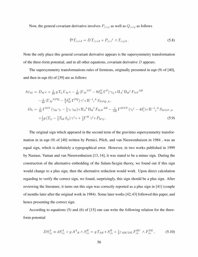
Now, the general covariant derivative involves P(1) ij as well as Q(1) ij as follows
D T(1) iA = DT(1) iA + P(1) ij ∧ T(1)jA . (5.8)
Note the only place this general covariant derivative appears is the supersymmetry transformation
of the three-form potential, and in all other equations, covariant derivative D appears.
The supersymmetry transformations rules of fermions, originally presented in eqn (9) of [40],
and then in eqn (6) of [39] are as follows
δψM = DM ϵ+ 120g Tii ΓM ϵ− 1
80(ΓM
NP − 8δNM ΓP ) γij ϵΠAiΠB
j FNPAB
− 160(ΓM
NPQ − 92δNM ΓPQ) γi ϵΠ−1
iA SNPQ ,A ,
δλi =132ΓMN (γkℓ γi − 1
5γi γkℓ) ϵΠA
k ΠBℓ FMN
AB − 1120
ΓMNP (γij − 4δji ) ϵΠ
−1jA SMNP ,A
+12g (Tij − 1
5Tkk δij) γ
j ϵ+ 12ΓM γj ϵ PM ij . (5.9)
The original sign which appeared in the second term of the gravitino supersymmetry transfor-
mation in in eqn (9) of [40] written by Pernici, Pilch, and van Nieuwenhuizen in 1984 , was an
equal sign, which is definitely a typographical error. However, in two works published in 1999
by Nastase, Vaman and van Nieuwenhuizen [13, 14], it was stated to be a minus sign. During the
construction of the alternative embedding of the Salam-Sezgin theory, we found out if this sign
would change to a plus sign, then the alternative reduction would work. Upon direct calculation
regarding to verify the correct sign, we found, surprisingly, this sign should be a plus sign. After
reviewing the literature, it turns out this sign was correctly reported as a plus sign in [41] (couple
of months later after the original work in 1984). Some later works [42,43] followed this paper, and
hence presenting the correct sign.
According to equations (5) and (6) of [15] one can write the following relation for the three-
form potential
DSA(3) ≡ dSA(3) + g AAB ∧ SB(3) = g TAB ∗ SB(3) + 18εABCDE F
BC(2) ∧ FDE
(2) , (5.10)
56
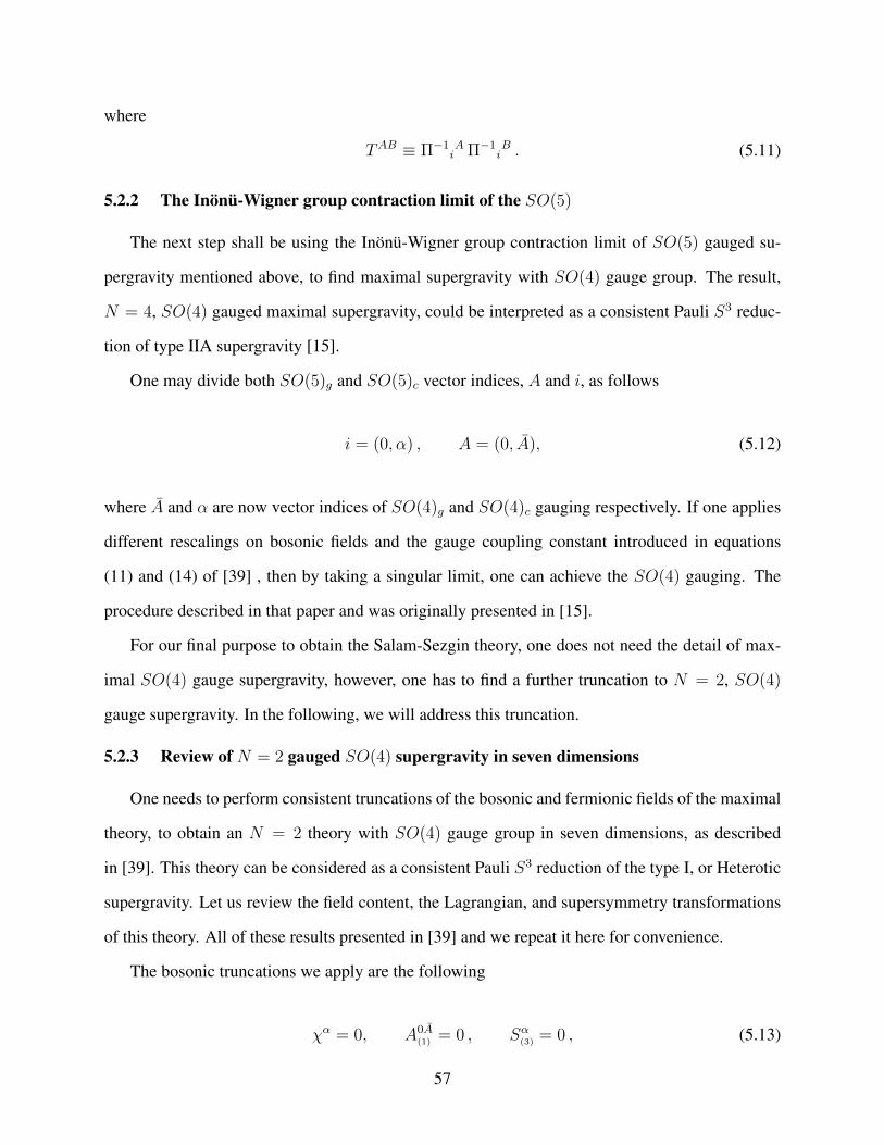
where
TAB ≡ Π−1iAΠ−1
iB . (5.11)
5.2.2 The Inönü-Wigner group contraction limit of the SO(5)
The next step shall be using the Inönü-Wigner group contraction limit of SO(5) gauged su-
pergravity mentioned above, to find maximal supergravity with SO(4) gauge group. The result,
N = 4, SO(4) gauged maximal supergravity, could be interpreted as a consistent Pauli S3 reduc-
tion of type IIA supergravity [15].
One may divide both SO(5)g and SO(5)c vector indices, A and i, as follows
i = (0, α) , A = (0, A), (5.12)
where A and α are now vector indices of SO(4)g and SO(4)c gauging respectively. If one applies
different rescalings on bosonic fields and the gauge coupling constant introduced in equations
(11) and (14) of [39] , then by taking a singular limit, one can achieve the SO(4) gauging. The
procedure described in that paper and was originally presented in [15].
For our final purpose to obtain the Salam-Sezgin theory, one does not need the detail of max-
imal SO(4) gauge supergravity, however, one has to find a further truncation to N = 2, SO(4)
gauge supergravity. In the following, we will address this truncation.
5.2.3 Review of N = 2 gauged SO(4) supergravity in seven dimensions
One needs to perform consistent truncations of the bosonic and fermionic fields of the maximal
theory, to obtain an N = 2 theory with SO(4) gauge group in seven dimensions, as described
in [39]. This theory can be considered as a consistent Pauli S3 reduction of the type I, or Heterotic
supergravity. Let us review the field content, the Lagrangian, and supersymmetry transformations
of this theory. All of these results presented in [39] and we repeat it here for convenience.
The bosonic truncations we apply are the following
χα = 0, A0A(1) = 0 , Sα(3) = 0 , (5.13)
57
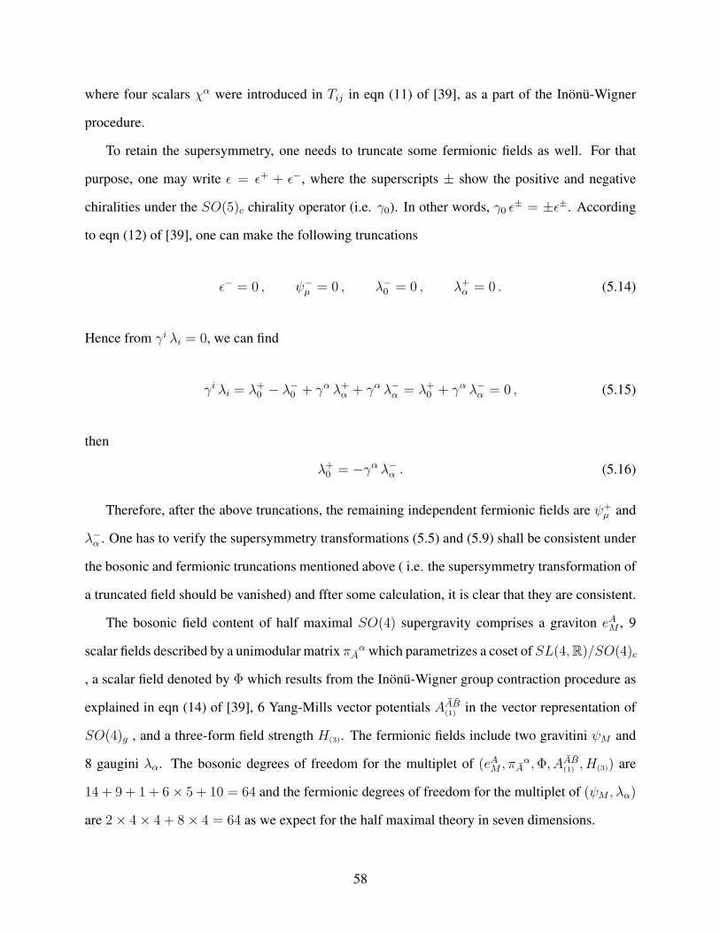
where four scalars χα were introduced in Tij in eqn (11) of [39], as a part of the Inönü-Wigner
procedure.
To retain the supersymmetry, one needs to truncate some fermionic fields as well. For that
purpose, one may write ϵ = ϵ+ + ϵ−, where the superscripts ± show the positive and negative
chiralities under the SO(5)c chirality operator (i.e. γ0). In other words, γ0 ϵ± = ±ϵ±. According
to eqn (12) of [39], one can make the following truncations
ϵ− = 0 , ψ−µ = 0 , λ−0 = 0 , λ+α = 0 . (5.14)
Hence from γi λi = 0, we can find
γi λi = λ+0 − λ−0 + γα λ+α + γα λ−α = λ+0 + γα λ−α = 0 , (5.15)
then
λ+0 = −γα λ−α . (5.16)
Therefore, after the above truncations, the remaining independent fermionic fields are ψ+µ and
λ−α . One has to verify the supersymmetry transformations (5.5) and (5.9) shall be consistent under
the bosonic and fermionic truncations mentioned above ( i.e. the supersymmetry transformation of
a truncated field should be vanished) and ffter some calculation, it is clear that they are consistent.
The bosonic field content of half maximal SO(4) supergravity comprises a graviton eAM , 9
scalar fields described by a unimodular matrix πAα which parametrizes a coset of SL(4,R)/SO(4)c
, a scalar field denoted by Φ which results from the Inönü-Wigner group contraction procedure as
explained in eqn (14) of [39], 6 Yang-Mills vector potentials AAB(1) in the vector representation of
SO(4)g , and a three-form field strength H(3). The fermionic fields include two gravitini ψM and
8 gaugini λα. The bosonic degrees of freedom for the multiplet of (eAM , πAα,Φ, AAB(1) , H(3)) are
14 + 9 + 1 + 6× 5 + 10 = 64 and the fermionic degrees of freedom for the multiplet of (ψM , λα)
are 2× 4× 4 + 8× 4 = 64 as we expect for the half maximal theory in seven dimensions.
58
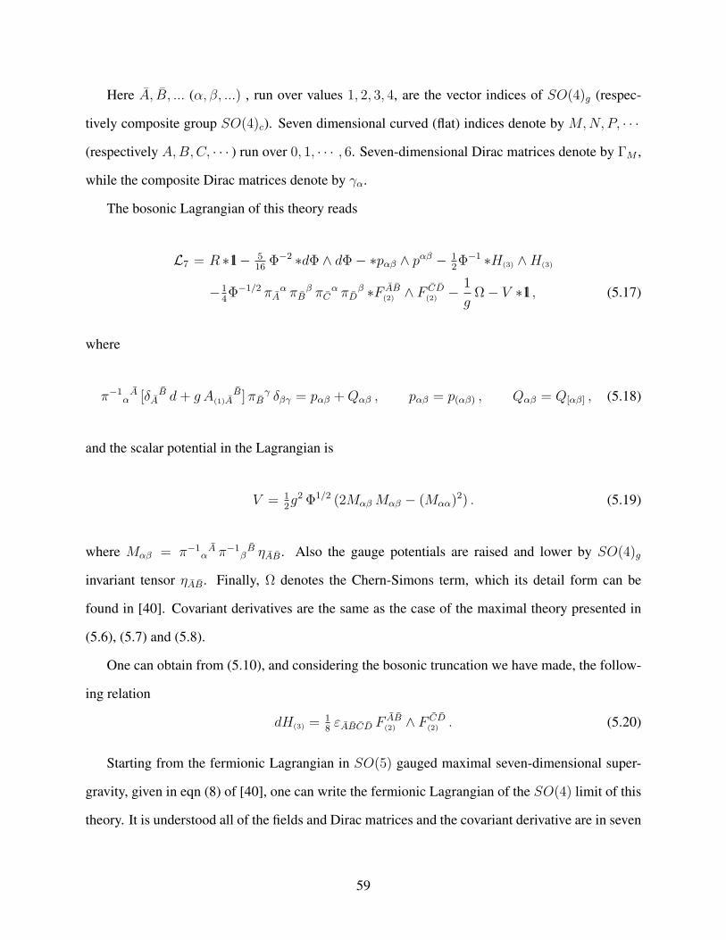
Here A, B, ... (α, β, ...) , run over values 1, 2, 3, 4, are the vector indices of SO(4)g (respec-
tively composite group SO(4)c). Seven dimensional curved (flat) indices denote by M,N,P, · · ·
(respectively A,B,C, · · · ) run over 0, 1, · · · , 6. Seven-dimensional Dirac matrices denote by ΓM ,
while the composite Dirac matrices denote by γα.
The bosonic Lagrangian of this theory reads
L7 = R ∗1l− 516Φ−2 ∗dΦ ∧ dΦ− ∗pαβ ∧ pαβ − 1
2Φ−1 ∗H(3) ∧H(3)
−14Φ−1/2 πA
α πBβ πC
α πDβ ∗F AB
(2) ∧ F CD(2) − 1
gΩ− V ∗1l , (5.17)
where
π−1αA [δA
B d+ g A(1)AB] πB
γ δβγ = pαβ +Qαβ , pαβ = p(αβ) , Qαβ = Q[αβ] , (5.18)
and the scalar potential in the Lagrangian is
V = 12g2Φ1/2 (2MαβMαβ − (Mαα)
2) . (5.19)
where Mαβ = π−1αA π−1
βB ηAB. Also the gauge potentials are raised and lower by SO(4)g
invariant tensor ηAB. Finally, Ω denotes the Chern-Simons term, which its detail form can be
found in [40]. Covariant derivatives are the same as the case of the maximal theory presented in
(5.6), (5.7) and (5.8).
One can obtain from (5.10), and considering the bosonic truncation we have made, the follow-
ing relation
dH(3) =18εABCD F
AB(2) ∧ F CD
(2) . (5.20)
Starting from the fermionic Lagrangian in SO(5) gauged maximal seven-dimensional super-
gravity, given in eqn (8) of [40], one can write the fermionic Lagrangian of the SO(4) limit of this
theory. It is understood all of the fields and Dirac matrices and the covariant derivative are in seven
59
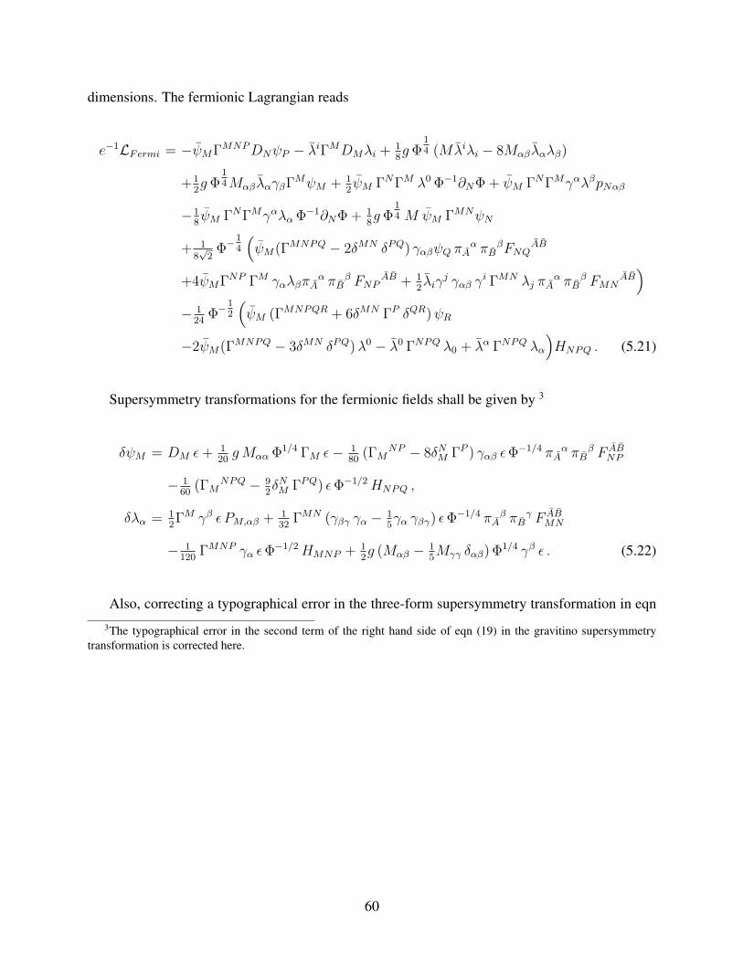
dimensions. The fermionic Lagrangian reads
e−1LFermi = −ψMΓMNPDNψP − λiΓMDMλi +18gΦ
14 (Mλiλi − 8Mαβλαλβ)
+12gΦ
14MαβλαγβΓ
MψM + 12ψM ΓNΓM λ0Φ−1∂NΦ + ψM ΓNΓMγαλβpNαβ
−18ψM ΓNΓMγαλαΦ
−1∂NΦ + 18gΦ
14 M ψM ΓMNψN
+ 18√2Φ−1
4
(ψM(ΓMNPQ − 2δMN δPQ) γαβψQ πA
α πBβFNQ
AB
+4ψMΓNP ΓM γαλβπAα πB
β FNPAB + 1
2λiγ
j γαβ γi ΓMN λj πA
α πBβ FMN
AB)
− 124Φ−1
2
(ψM (ΓMNPQR + 6δMN ΓP δQR)ψR
−2ψM(ΓMNPQ − 3δMN δPQ)λ0 − λ0 ΓNPQ λ0 + λα ΓNPQ λα
)HNPQ . (5.21)
Supersymmetry transformations for the fermionic fields shall be given by 3
δψM = DM ϵ+ 120gMααΦ
1/4 ΓM ϵ− 180(ΓM
NP − 8δNM ΓP ) γαβ ϵΦ−1/4 πA
α πBβ F AB
NP
− 160(ΓM
NPQ − 92δNM ΓPQ) ϵΦ−1/2HNPQ ,
δλα = 12ΓM γβ ϵ PM,αβ +
132ΓMN (γβγ γα − 1
5γα γβγ) ϵΦ
−1/4 πAβ πB
γ F ABMN
− 1120
ΓMNP γα ϵΦ−1/2HMNP + 1
2g (Mαβ − 1
5Mγγ δαβ) Φ
1/4 γβ ϵ . (5.22)
Also, correcting a typographical error in the three-form supersymmetry transformation in eqn
3The typographical error in the second term of the right hand side of eqn (19) in the gravitino supersymmetrytransformation is corrected here.
60
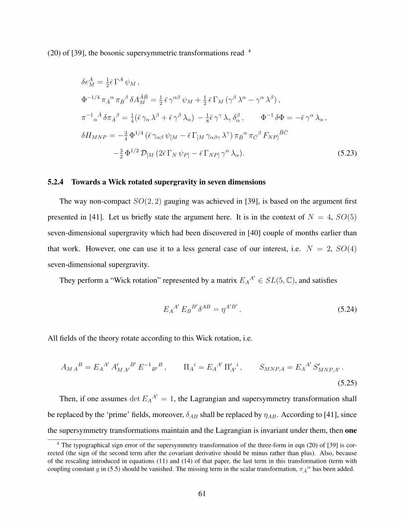
(20) of [39], the bosonic supersymmetric transformations read 4
δeAM = 12ϵΓA ψM ,
Φ−1/4 πAα πB
β δAABM = 12ϵ γαβ ψM + 1
2ϵΓM (γβ λα − γα λβ) ,
π−1αA δπA
β = 14(ϵ γα λ
β + ϵ γβ λα) − 18ϵ γγ λγ δ
βα , Φ−1 δΦ = −ϵ γα λα ,
δHMNP = −34Φ1/4 (ϵ γαβ ψ[M − ϵΓ[M γαβγ λ
γ)πBα πC
β FNP ]BC
−32Φ1/2D[M (2ϵΓN ψP ] − ϵΓNP ] γ
α λα). (5.23)
5.2.4 Towards a Wick rotated supergravity in seven dimensions
The way non-compact SO(2, 2) gauging was achieved in [39], is based on the argument first
presented in [41]. Let us briefly state the argument here. It is in the context of N = 4, SO(5)
seven-dimensional supergravity which had been discovered in [40] couple of months earlier than
that work. However, one can use it to a less general case of our interest, i.e. N = 2, SO(4)
seven-dimensional supergravity.
They perform a “Wick rotation” represented by a matrix EAA′ ∈ SL(5,C), and satisfies
EAA′EB
B′δAB = ηA
′B′. (5.24)
All fields of the theory rotate according to this Wick rotation, i.e.
AM AB = EA
A′A′M A′
B′E−1
B′B , ΠA
i = EAA′Π′A′i , SMNP,A = EA
A′S ′MNP,A′ .
(5.25)
Then, if one assumes detEAA′= 1, the Lagrangian and supersymmetry transformation shall
be replaced by the ‘prime’ fields, moreover, δAB shall be replaced by ηAB. According to [41], since
the supersymmetry transformations maintain and the Lagrangian is invariant under them, then one4 The typographical sign error of the supersymmetry transformation of the three-form in eqn (20) of [39] is cor-
rected (the sign of the second term after the covariant derivative should be minus rather than plus). Also, becauseof the rescaling introduced in equations (11) and (14) of that paper, the last term in this transformation (term withcoupling constant g in (5.5) should be vanished. The missing term in the scalar transformation, πA
α has been added.
61
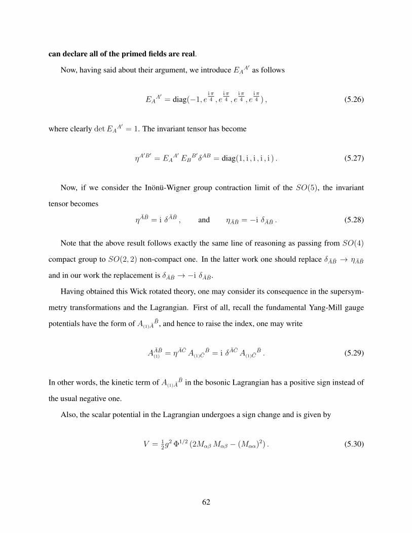
can declare all of the primed fields are real.
Now, having said about their argument, we introduce EAA′ as follows
EAA′
= diag(−1, eiπ4 , e
iπ4 , e
iπ4 , e
iπ4 ) , (5.26)
where clearly detEAA′
= 1. The invariant tensor has become
ηA′B′
= EAA′EB
B′δAB = diag(1, i , i , i , i ) . (5.27)
Now, if we consider the Inönü-Wigner group contraction limit of the SO(5), the invariant
tensor becomes
ηAB = i δAB , and ηAB = −i δAB . (5.28)
Note that the above result follows exactly the same line of reasoning as passing from SO(4)
compact group to SO(2, 2) non-compact one. In the latter work one should replace δAB → ηAB
and in our work the replacement is δAB → −i δAB.
Having obtained this Wick rotated theory, one may consider its consequence in the supersym-
metry transformations and the Lagrangian. First of all, recall the fundamental Yang-Mill gauge
potentials have the form of A(1)AB, and hence to raise the index, one may write
AAB(1) = ηAC A(1)CB = i δAC A(1)C
B . (5.29)
In other words, the kinetic term of A(1)AB in the bosonic Lagrangian has a positive sign instead of
the usual negative one.
Also, the scalar potential in the Lagrangian undergoes a sign change and is given by
V = 12g2Φ1/2 (2MαβMαβ − (Mαα)
2) . (5.30)
62
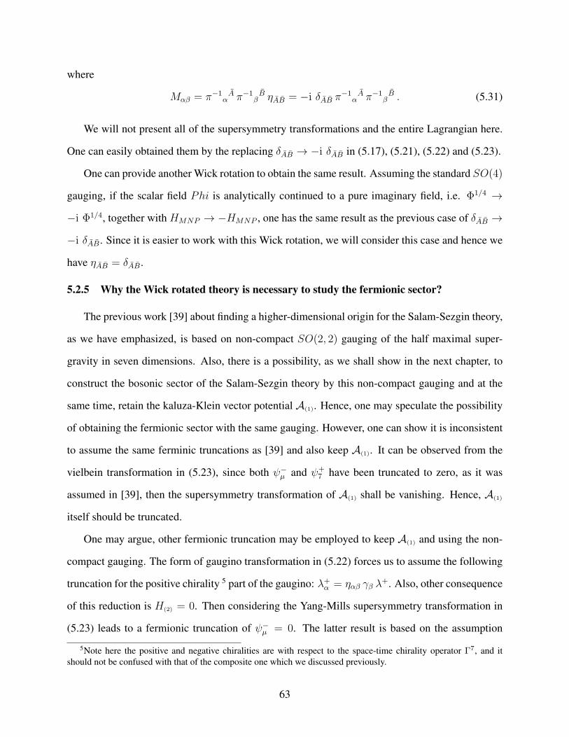
where
Mαβ = π−1αA π−1
βB ηAB = −i δAB π
−1αA π−1
βB . (5.31)
We will not present all of the supersymmetry transformations and the entire Lagrangian here.
One can easily obtained them by the replacing δAB → −i δAB in (5.17), (5.21), (5.22) and (5.23).
One can provide another Wick rotation to obtain the same result. Assuming the standard SO(4)
gauging, if the scalar field Phi is analytically continued to a pure imaginary field, i.e. Φ1/4 →
−i Φ1/4, together with HMNP → −HMNP , one has the same result as the previous case of δAB →
−i δAB. Since it is easier to work with this Wick rotation, we will consider this case and hence we
have ηAB = δAB.
5.2.5 Why the Wick rotated theory is necessary to study the fermionic sector?
The previous work [39] about finding a higher-dimensional origin for the Salam-Sezgin theory,
as we have emphasized, is based on non-compact SO(2, 2) gauging of the half maximal super-
gravity in seven dimensions. Also, there is a possibility, as we shall show in the next chapter, to
construct the bosonic sector of the Salam-Sezgin theory by this non-compact gauging and at the
same time, retain the kaluza-Klein vector potential A(1). Hence, one may speculate the possibility
of obtaining the fermionic sector with the same gauging. However, one can show it is inconsistent
to assume the same ferminic truncations as [39] and also keep A(1). It can be observed from the
vielbein transformation in (5.23), since both ψ−µ and ψ+
7 have been truncated to zero, as it was
assumed in [39], then the supersymmetry transformation of A(1) shall be vanishing. Hence, A(1)
itself should be truncated.
One may argue, other fermionic truncation may be employed to keep A(1) and using the non-
compact gauging. The form of gaugino transformation in (5.22) forces us to assume the following
truncation for the positive chirality 5 part of the gaugino: λ+α = ηαβ γβ λ+. Also, other consequence
of this reduction is H(2) = 0. Then considering the Yang-Mills supersymmetry transformation in
(5.23) leads to a fermionic truncation of ψ−µ = 0. The latter result is based on the assumption
5Note here the positive and negative chiralities are with respect to the space-time chirality operator Γ7, and itshould not be confused with that of the composite one which we discussed previously.
63
from the bosonic sector where the Chern-Simons contribution vanishes if A12(1) = ±A34
(1). If one
considers the supersymmetry transformation of ψ+7 in (5.22), then since H(2) = 0, then one has
δψ+7 ∼ g(χ12 + χ34) γ12ϵ.6 In addition to this, since the fermionic degrees of freedom are 20, then
one needs to truncate the latter field (since it is not possible to make this field proportional to other
fermionic fields), meaning that δA(1) = 0, or A(1) should be truncated. This argument shows the
bosonic and fermionic ansatz, presented in [39], is the only consistent possibility if one considers
SO(2, 2) non-compact gauging in seven dimensions.
It is worth to mention that the truncation discussed in [39] does not consistent with the compact
SO(4) gauging. To see this, one may find the supersymmetry transformation of the field ψ−µ , which
is truncated to zero in that work, is non-vanishing. According to (5.22), there is a Mαα = ηαα
contribution in that transformation, which actually becomes zero for the case of SO(2, 2), but it
shall be 4 in the case of SO(4) gauging. It clearly indicates that this scheme of truncations does
not consistent with the compact gauging, and one needs to use the non-compact one, as it was
employed in [39].
In the next section, we perform a Kaluza-Klein circle down to six dimensions and consider the
bosonic truncations and equations of motion.
5.3 The Kaluza-Klein circle reduction to six dimensions: bosonic sector
The Kaluza-Klein circle reduction is a standard calculation which we presented in the chapter
2. Using those results, one can write the metric ansatz as follows
ds27 = e2αφ ds26 + e−8αφ (dz +A(1))2 , (5.32)
where φ is a “breathing mode”, and α2 = 140
. Also in this section, we insert hat on seven-
dimensional fields to distinguish them from the six-dimensional ones. The bosonic ansätze for
a circle reduction are standard and shall be addressed in the next part.
6The scalar has been ignored, this is why “∼” has been used
64
5.3.1 The ansätze for gauge potentials
For obtaining the Salam-Sezgin theory, one does not need six gauge potentials of the SO(4)
half maximal theory, thus one may truncate them. We consider a consistent truncation where
only the maximal Abelian subgroup, i.e. U(1)2, of SO(4)g gauged Yang-Mills fields are retained.
Namely, A12(1) = A(1) and A34
(1) = A′(1) are kept. Also, one may truncate all scalars in the coset
SL(4,R)/SO(4), i.e. πAα = δAα. Consequently, with the assumption of keeping the compact
gauge group SO(4), then Mαβ = δαβ . Obviously, this truncation is consistent with all equations
of motion. Having assumed this truncation, and using (5.20), then one can write
dH(3) = F(2) ∧ F ′(2) , F(2) = dA(1), F ′
(2) = dA′(1) . (5.33)
Based on the above relations, one can write
dH(3) =12d(F(2) ∧ A′
(1) + A(1) ∧ F ′(2)) , (5.34)
and hence
H(3) = dB(2) +12F(2) ∧ A′
(1) +12F ′
(2) ∧ A(1) . (5.35)
The ansätze for the Kaluza-Klein circle reduction for the bosonic fields are standard and can
be written as follows
H(3) = H(3) +H(2) ∧ (dz +A(1)),
A(1) = A(1) + χdz, A′(1) = A′
(1) + χ′ dz,
B(2) = B(2) +B(1) ∧ dz,
F(2) = F(2) + dχ ∧ (dz +A(1)), F ′(2) = F ′
(2) + dχ′ ∧ (dz +A(1)) . (5.36)
65
Therefore, one may find the following relations for six-dimensional fields
H(3) = dB(2) − dB(1) ∧ A(1) +12dA(1) ∧ A′
(1) +12dA′
(1) ∧ A(1)
−12(χ′dA(1) + χdA′
(1)) ∧ A(1) − 12(A(1) ∧ dχ′ + A′
(1) ∧ dχ) ∧ A(1),
H(2) = dB(1) +12(χ′dA(1) + χdA′
(1) + A′(1) ∧ dχ+ A(1) ∧ dχ′),
F(2) = dA(1) − dχ ∧ A(1), F ′(2) = dA′
(1) − dχ′ ∧ A(1), F(2) = dA(1) . (5.37)
Writing in the flat indices, one can find the following relations between components of seven-
and six- dimensional fields
Habc = e−3αφHabc, Hab7 = e2αφHab,
Aa = e−αφ (Aa − χAa), A′a = e−αφ (A′
a − χ′ Aa), A7 = e4αφ χ, A′7 = e4αφ χ′
e = e2αφ e . (5.38)
In addition to this, one can easily obtain relations between the components of seven- and six-
dimensional fields in the curved indices
H(3)µνρ = H(3)µνρ + 3H(2) [µν Aρ], H(3)µνz = H(2)µν ,
Aµ = Aµ, A′µ = A′
µ, Az = χ, A′z = χ′,
B(2)µν = B(2)µν , B(2)µz = B(1)µ . (5.39)
At this stage, following [45], a re-parametrization of two scalar fields Φ and φ is introduced as
follows
Φ = e25ψ−4
5ϕ , 20αφ = −2ψ − ϕ . (5.40)
66
With these preliminaries, the six-dimensional bosonic Lagrangian becomes
L6 = R∗1l− 14∗dϕ ∧ dϕ− 1
4∗dψ ∧ dψ − 1
2e12ϕ+ψ ∗F (2) ∧ F(2) − 1
2eϕ ∗H(3) ∧H(3)
−12e12ϕ−ψ ∗H(2) ∧H(2) +
12e12ϕ (∗F(2) ∧ F(2) + ∗F ′
(2) ∧ F ′(2))
+14e−ψ (∗dχ ∧ dχ+ ∗dχ′ ∧ dχ′)− Ω(6)
g− V ∗1l , (5.41)
where
V = 4g2e−12ϕ , (5.42)
and Ω(6) is the Chern-Simons term in six dimensions which shall be studied in the next subsection.
Note that the Yang-Mills kinetic terms have a wrong sign.
5.3.2 The Chern-Simons term in seven dimensions
Let us calculate the Chern-Simons variation for the Abelian truncation, i.e. A(2) = A12(2), A
′(2) =
A34(2). Since all of the fields in this part is seven-dimensional, then we omit the hat for simplicity.
The expression we have used here to calculate the Chern-Simons term is eqn (10) of [40]. Since the
normalization convention for the trace operator does not specify clearly in the latter, we generally
assume
Tr(F ∧ F ) = c F ij ∧ F ji , (5.43)
where this c is either 1 or 12. We have the following relations for δΩ(3)
δΩ(3) = 4c2(F ∧ F + F ′ ∧ F ′) ∧ (F ∧ δA+ F ′ ∧ δA′)
= 4c2(F ∧ F ∧ F ∧ δA+ F ∧ F ∧ F ′ ∧ δA′
+F ′ ∧ F ′ ∧ F ∧ δA+ F ′ ∧ F ′ ∧ F ′ ∧ δA′) . (5.44)
Also, δΩ(5) shall be written as follows
δΩ(5) = 2c (F ∧ F ∧ F ∧ δA+ F ′ ∧ F ′ ∧ F ′ ∧ δA′) . (5.45)
67
Now, combining the above relations, one may find the following relation for the Chern-Simons
variation
δΩ(7) = 2δΩ(5) − δΩ(3) = 4c[(1− c)F ∧ F ∧ F ∧ δA+ (1− c)F ′ ∧ F ′ ∧ F ′ ∧ δA′
−cF ∧ F ∧ F ′ ∧ δA′ − cF ′ ∧ F ′ ∧ F ∧ δA]. (5.46)
Therefore, for the specific value of c = 12, we have the following
δΩ(7) = F ∧ F ∧ F ∧ δA+ F ′ ∧ F ′ ∧ F ′ ∧ δA′
−F ∧ F ∧ F ′ ∧ δA′ − F ′ ∧ F ′ ∧ F ∧ δA . (5.47)
After some algebra, one finds the 7D Chern-Simons term, up to a total derivative is
Ω(7) =14F ∧ F ∧ F ∧ A+ 1
4F ′ ∧ F ′ ∧ F ′ ∧ A′ − 1
2F ∧ F ∧ F ′ ∧ A′ . (5.48)
The above relation for seven-dimensional Chern-Simons term can be vanished in specific cases,
e.g. F = ±F ′. Therefore, we apply a further truncation and assume A = A′, or in six dimensions
A = A′ and χ = χ′ .
5.3.3 The bosonic equations of motion
Now, we shall find equations of motion of the six dimensional theory derived from the La-
grangian above (5.41). To ensure the truncation we have imposed on the Yang-Mills fields, i.e.
A = A′ and χ = χ′ is consistent, we present equations of motion for both gauge potentials and
the axions, and then we will deduce the above mentioned truncation is consistent with the equa-
tions we will present. However, the Chern-Simons term is vanishing according to the argument
presented in the previous part. First we state scalar equations of motion
ϕ = 14e12ϕ+ψ F2
(2) +16eϕH2
(3) +14e12ϕ−ψH2
(2) − 14e12ϕ (F 2
(2) + F ′2(2))− 4g2e−
12ϕ,
ψ = 12e12ϕ+ψ F2
(2) − 12e12ϕ−ψH2
(2) +12e−ψ
((∂χ)2 + (∂χ′)2
). (5.49)
68
Next, we consider equations of motion for one-form potentials A(1) and A′(1) as follows:
2d(e12ϕ ∗ F(2)) = −d(e
12ϕ−ψ ∗H(2)χ
′)− e12ϕ−ψ ∗H(2) ∧ dχ′
−d(eϕ ∗H(3) ∧ (A′
(1) − χ′A(1)))+ eϕ ∗H(3) ∧ F ′
(2) ,
2d(e12ϕ ∗ F ′
(2)) = −d(e12ϕ−ψ ∗H(2)χ)− e
12ϕ−ψ ∗H(2) ∧ dχ
−d(eϕ ∗H(3) ∧ (A(1) − χA(1))
)+ eϕ ∗H(3) ∧ F(2) . (5.50)
The equation of motion for the Kaluza-Klein vector potential A(1) reads
d(e12ϕ+ψ ∗ F(2)
)= −eϕ ∗H(3) ∧
[dB(1) − 1
2(χ′dA(1) + χdA′
(1) + A(1) ∧ dχ′ + A′(1) ∧ dχ)
]+1
2e−
12ϕ (∗F(2) ∧ dχ+ ∗F ′
(2) ∧ dχ′) . (5.51)
Next, we consider equations of motion for potentials B(1) and B(2) in the following
d(e12ϕ−ψ ∗H(2)) = d(eϕ ∗H(3) ∧ A(1)),
d(eϕ ∗H(3)) = 0 . (5.52)
Finally, equations of motion for axionic scalar fields χ and χ′ are
d(e−ψ ∗ dχ) = eϕ ∗H(3) ∧ dA′(1) ∧ A(1) − d(eϕ ∗H(3) ∧ A′
(1) ∧ A(1))− e12ϕ−ψ ∗H(2) ∧ dA′
(1)
−d(e12ϕ−ψ ∗H(2) ∧ A′
(1))− d(e12ϕ ∗ F(2) ∧ A(1)) ,
d(e−ψ′ ∗ dχ′) = eϕ ∗H(3) ∧ dA(1) ∧ A(1) − d(eϕ ∗H(3) ∧ A(1) ∧ A(1))− e
12ϕ−ψ ∗H(2) ∧ dA(1)
−d(e12ϕ−ψ ∗H(2) ∧ A(1))− d(e
12ϕ ∗ F ′
(2) ∧ A(1)) . (5.53)
Now it is a straightforward task to check the ansazt A = A′ and χ = χ′ is consistent with
the above mention equations. therefore, it is possible to find more convenient relations. Plugging
69
(5.52) in (5.50), one can obtain the following relations for the six-dimensional field strengths
d(e12ϕ ∗ F(2)) = −e
12ϕ−ψ ∗H(2) ∧ dχ+ eϕ ∗H(3) ∧ F(2) . (5.54)
Using the equations (5.50) and (5.52), one can find the following equations of motion for the
axionic scalar field
d(e−ψ ∗ dχ) = eϕ ∗H(3) ∧ dA(1) ∧ A(1) − e12ϕ−ψ ∗H(2) ∧ (2dA(1) − dχ ∧ dA(1))
−e12ϕ ∗ F(2) ∧ dA(1) . (5.55)
The equation of motion for Kaluza-Klein vector field strengths, can be easily found by using
H(2) relation from (5.37)
d(e12ϕ+ψ ∗ F(2)
)= −eϕ ∗H(3) ∧H(2) + e−
12ϕ ∗ F(2) ∧ dχ . (5.56)
5.3.4 The bosonic truncations
There is only one scalar field appears in the Salam-Sezgin theory, while the theory presented in
the last part has three scalars ϕ, ψ and χ . Hence, one needs to perform a consistent truncation of
these scalars. The axions were truncated to zero in [39], but, if these fields would be just constant
numbers, then, obviously, they did not contribute in the kinetic part of the Lagrangian. Upon
investigation in the supersymmetry transformations, one has to truncate both A and A′ to zero.
However, since the covariant derivative depends on the gauge field, one needs to keep the axion,
but one may assume it is not a dynamical field, but a constant number to be determined by
supersymmetry transformations.
In that sense, one can retain the standard gauging in the covariant derivative, however, instead
of the usual Yang-Mills vector potential, one has the Kaluza-Klein vector potential A(1) as a gauge
field.
Now, we may check whether our proposed truncation is consistent with the bosonic equations
70
of motion. It can be easily verified that equation of motion for the axion (5.55) , and also the field
strength F(2) (5.50) are trivially satisfied. The remaining equations after this truncation shall be
ϕ = 14e12ϕ+ψ F2
(2) +16eϕH2
(3) +14e12ϕ−ψH2
(2) − 4g2e−12ϕ,
ψ = 12e12ϕ+ψ F2
(2) − 12e12ϕ−ψH2
(2),
d(e12ϕ−ψ ∗H(2)) = −eϕ ∗H(3) ∧ F(2),
d(eϕ ∗H(3)) = 0,
d(e12ϕ+ψ ∗ F(2)
)= −eϕ ∗H(3) ∧H(2) . (5.57)
Also, the six-dimensional bosonic Lagrangian has the following form
L6 = R∗1l− 14∗dϕ ∧ dϕ− 1
4∗dψ ∧ dψ − 1
2e12ϕ+ψ ∗F (2) ∧ F(2) − 1
2eϕ ∗H(3) ∧H(3)
−12e12ϕ−ψ ∗H(2) ∧H(2) − 4g2 e−
12ϕ ∗1l . (5.58)
This is still not the bosonic Salam-Sezgin Lagrangian, and one more truncation is needed to
this theory be achieved. Assume the scalar field ψ is vanishing, and at the same time, F2(2) = H2
(2).
They are consistent with equations of motion (5.57). Therefore, due to the re-parametrization given
in (5.40) one has
Φ = e−45ϕ , 20αφ = −ϕ , Φ = e16αφ . (5.59)
Finally, the bosonic Lagrangian shall be that of the Salam-Sezgin
L6 = R∗1l− 14∗dϕ ∧ dϕ− e
12ϕ ∗F (2) ∧ F(2) − 1
2eϕ ∗H(3) ∧H(3) − 4g2 e−
12ϕ ∗1l , (5.60)
with the rescaling of F2(2) = H2
(2) = 2 F 2(2), where F(2) is the field strength in the Salam-Sezgin
71
theory. Let us summarize all the bosonic truncations we have found so far
ψ = 0, Φ = e16αφ, 20αφ = −ϕ, πAα = δA
α, Mαβ = δαβ,
F AB = 0, Aa = A′a = −χAa, A7 = A′
7 = χ, F2(2) = H2
(2) = 2 F 2(2), χ = χ′ = const. ,
H(3) = dB(2) − dB(1) ∧ A(1), H(2) = dB(1), F(2) = dA(1). (5.61)
Since F2(2) = H2
(2), one has options of F(2) = ±H(2). The important question of which sign should
be chosen, is not answered by the bosonic sector, and it will be determined by the supersymmetry
considerations. Also, the constant value of the axion shall be determined by the supersymmetry
transformations as well.
5.3.5 The supersymmetry transformations?
We stated in 5.2.4 that the starting point theory in seven dimensions is a Wick rotated theory
which we may find it by δAB → −i δAB Wick rotation. However, the reality condition for the
fermionic fields becomes vague here. In spite of that, we found a fermionic truncation for the
circle reduction of the Wick rotated theory and we could recover the fermionic Lagrangian of the
Salam-Sezgin theory. This is a very encouraging hint about the presence of such an exotic theory
in seven dimensions.
We do not present our calculations in the fermionic sector, since the seven dimensional theory
is not yet rigorously proved to be existed.
5.4 Final remarks
It is instructive to find out the embedding of the seven-dimensional metric in ten dimensions.
Recall our Wick rotation δAB → −i δAB, or the other option Φ1/4 → −i Φ1/4. One needs to
investigate the consequences of this odd choice.
The embedding of seven-dimensional metric ansatz to ten dimensions, as in eqn (46) of [15],
is as follows
ds210 = g−14 Φ
316 ∆
14(ds27 + g−2Φ−1
2 ∆−1M−1αβ Dµ
αDµβ). (5.62)
72
Hence, after applying either of the above Wick rotations, one can write
ds210 = Ω(ds27 − g−2Φ−1
2 DµαDµα). (5.63)
It means the dimensional reduction has been performed on three time-like coordinates instead
of the usual space-like reduction. One may conclude this reduction is a case of Hull’s [50, 51]
program about time-like reduction. Actually he found there is an exotic type IIA in (6,4) signature,
i.e. 6 space-like and 4 time-like coordinates [50]. Then one may speculate the Wick rotated
supergravity we are looking for, is actually the three time-like reduction of type IIA (6,4).
This is an interesting possibility and further work is needed to find a more elaborated connec-
tion between the Wick rotated seven dimensional supergravity and the time-like reduction.
73
6. PAULI S2 REDUCTION OF THE SALAM-SEZGIN THEORY
6.1 Introduction
In the previous chapter we saw an alternative higher dimensional origin for the Salam-Sezgin
theory where the Kaluza-Klein vector potential A(1) is non-zero. As we have emphasized there, the
reason for keeping this field is to use the “Hopf fibration technique” and to find a group-theoretical
explanation for the consistent Pauli S2 reduction of the Salam-Sezgin theory, constructed by Gib-
bons and Pope in [38].
The first step towards using the Hopf fibration technique, is starting from a seven-dimensional
theory. As we have discussed in the previous chapter, if one considers just the bosonic sector,
this theory can be SO(2, 2) gauged half maximal, i.e. N = 2 seven-dimensional supergravity. This
theory has been investigated in [39], and it may be derived from type I or Heterotic string theory
as it was shown in [15].
The next step is performing the Kaluza-Klein S1 reduction down to six dimensions to obtain
a non-chiral N = (1, 1) supergravity. Then, one may apply consistent truncations to obtain the
Salam-Sezgin theory. However, the difference between the six-dimensional bosonic truncation
imposed in [39] and ours is the Kaluza-Klein field strength F(2) and two-form field strength H(2)
in one hand and the Yang-Mills field strengths F 12(2) and F 34
(2) in the other hand. Let us compare two
truncations in the following
Truncation given by [39] : F(2) = H(2) = 0 , F 12(2) = −F 34
(2) ,
Our truncation : F(2) = −H(2) , F 12(2) = F 34
(2) = 0 . (6.1)
Note both of these truncations are consistent and give rise to the Salam-Sezgin theory in the bosonic
sector.
Then one needs to perform an SU(2) DeWitt reduction of the seven-dimensional theory to
obtain a four-dimensional one [44]. Now, having obtained a consistent reduction of the Salam-
74
Sezgin theory with its Dirac monopole A(1), it is a straightforward calculation to write the the
SU(2) as a U(1) Hopf fibration over S2 . The crucial point here is, the ansatz we may write in the
Hopf fibration manner, should be consistent with the truncation we have applied in six dimensions
to obtain the Salam-Sezgin theory. As we will observe, this truncation is consistent with the Hopf
ansatz. Thus, one can read off the consistent S2 reduction of the Salam-Sezgin theory, and find
the exact same results as [38] after some field rescalings. Therefore, by this method, we have a
group-theoretic understanding of why the Pauli S2 reduction of the Salam-Sezgin theory works.
In this chapter, we deal with fields in seven, six and four dimensions. To avoid ambiguity, the
convention is as follow. We insert a hat on seven-dimensional fields and four-dimensional ones are
appearing without any symbol on them everywhere. Especially in section 6.5, and where there is a
chance of an ambiguity, we shall insert a bar on six-dimensional quantities.
The rest of this chapter is organized as follows. In section 6.2, we shall consider the non-
compact SO(2, 2) half maximal seven-dimensional supergravity and perform some truncatuions.
In section 6.3, we perform a Kaluza-Klein S1 reduction followed by our bosonic truncations to
obtain the Salam-Sezgin theory. We perform an SU(2) DeWitt reduction in section 6.4, and we
consider the Hopf fibration technique in section 6.5 to find the S2 reduction of the Salam-Sezgin
theory. Also, we will verify the consistency of our ansatz by inserting it in six-dimensional equa-
tions of motion.
6.2 Truncation of N = 2 gauged SO(2, 2) supergravity in seven dimensions
The gauged SO(4) half maximal supergravity in seven dimensions, as we described in length
in chapter 5, can be obtained from maximal SO(5) seven-dimensional supergravity found in [40]
in two steps:
First, one may use the Inönü-Wigner group contraction limit of SO(5) gauged supergravity to
find a maximal supergravity (i.e. N = 4) with SO(4) gauge group.
Second, one may perform a consistent truncations on bosonic and fermionic fields of the max-
imal SO(4) theory to obtain a half maximal theory with N = 2, but with the same SO(4) gauging
in seven dimensions.
75
The entire Lagrangian and the supersymmetry transformations of seven-dimensional gauged
SO(4) half maximal supergravity were given in 5.2.3.
6.2.1 Pass to a non-compact SO(2, 2) gauging
As it was illustrated in [41], it is possible to pass from a compact Yang-Mills gauging to
a non-compact one. Following that idea, it was assumed in [39] the gauging can be the non-
compact SO(2, 2) rather than the compact SO(4) one. One needs to simply assume ηAB =
diag (1, 1,−1,−1).
The main motivation of choosing the non-compact gauging is obtaining the positive definite
potential of the Salam-Sezgin theory, which is one of the main obstacle to find a higher dimensional
embedding of this theory. According to a no-go theorem by Maldacena and Nunez [43], if the
lower-dimensional space-time has a positive definite potential, then the non-singular internal space
should be non-compact. This is why the non-compact group was chosen in [39].
Now, having described the bosonic part of the half maximal theory with non-compact SO(2, 2)
gauging in seven dimensions, one may perform a consistent bosonic truncation to find a simpler
theory in seven dimensions.
6.2.2 Truncation of SO(2, 2) half maximal theory in seven dimensions
If one interests in just the bosonic section of the Salam-Sezgin theory and its Pauli S2 reduction
down to four-dimensional space-time, then it is more convenient to impose truncations in seven-
dimensional SO(2, 2) half maximal theory, before performing the S1 Kaluza-Klein reduction. The
truncation is as follows
πAα = δA
α , AAB(1) = 0 . (6.2)
The above truncation is obviously consistent, i.e. the equations of motion of the bosonic La-
grangian (5.17) is consistent with them. The final bosonic Lagrangian after applying the above
truncations has become
L7 = R ∗1l− 516Φ−2 ∗dΦ ∧ dΦ− 1
2Φ−1 ∗H(3) ∧ H(3) − 4g2 Φ
12 ∗1l , (6.3)
76
where we insert hat on fields to emphasize they are seven-dimensional ones. Note we have used
the non-compact gauging to obtain the potential term, i.e. ηAB = diag (1, 1,−1,−1), and also
Mαβ = ηαβ , according to truncation of the scalar fields.
The Bianchi identity (5.20), after the above truncations reads
dH(3) = 0 . (6.4)
Now, one may perform the S1 Kaluza-Klein reduction to find the bosonic sector of the Salam-
Sezgin theory.
6.3 The Kaluza-Klein circle reduction down to six dimensions
The Kaluza-Klein circle reduction is a standard calculation which we presented in the chapter
2. Using these results, one can write the metric ansatz as follows
ds27 = e2αφ ds26 + e−8αφ (dz +A(1))2 , (6.5)
where φ is a “breathing mode”, and α2 = 140
.
Making use of the seven-dimensional Bianchi identity dH(3) = 0, one can write
H(3) = dB(2) . (6.6)
The ansätze for the Kaluza-Klein circle reduction for the bosonic fields are standard and can
be written as follows
B(2) = B(2) +B(1) ∧ dz , H(3) = H(3) +H(2) ∧ (dz +A(1)) , (6.7)
where
H(3) = dB(2) − dB(1) ∧ A(1) , H(2) = dB(1) , F(2) = dA(1) . (6.8)
The relations between the flat and curved components of seven- and six- dimensional fields are
77
as follows
Habc = e−3αφHabc, Hab7 = e2αφHab , e = e2αφ e
H(3)µνρ = H(3)µνρ + 3H(2) [µν Aρ], H(3)µνz = H(2)µν ,
B(2)µν = B(2)µν , B(2)µz = B(1)µ . (6.9)
The convenient re-parametrization of scalar fields is introduced again as follows
Φ = e25ψ−4
5ϕ , 20αφ = −2ψ − ϕ . (6.10)
Having obtained the circle reduction, the six-dimensional bosonic Lagrangian becomes
L6 = R∗1l− 14∗dϕ ∧ dϕ− 1
4∗dψ ∧ dψ − 1
2e12ϕ+ψ ∗F (2) ∧ F(2) − 1
2eϕ ∗H(3) ∧H(3)
−12e12ϕ−ψ ∗H(2) ∧H(2) − 4g2e−
12ϕ∗1l , (6.11)
Now, we shall find equations of motion of the six dimensional theory derived from the La-
grangian in (6.11). They are exactly as eqn (5.57).
At this stage, we impose truncations in six-dimensional fields to obtain the Salam-Sezgin the-
ory.
6.3.1 The bosonic truncations in six dimensions
The bosonic sector of the Salam-Sezgin theory can be achieved by the following truncations in
six dimensions
ψ = 0 , A(1) = −B(1) ≡ 1√2A(1) (6.12)
where A(1) is the gauge potential appears in the Salam-Sezgin theory. It is easy to check the above
ansatz is consistent with the six-dimensional equations we have found in (5.57).
Now, the six-dimensional bosonic Lagrangian in (6.11) becomes that of the Salam-Sezgin the-
78
ory
LSS = R ∗1l− 14∗dϕ ∧ dϕ− 1
2e12ϕ ∗F(2) ∧ F(2) − 1
2eϕ ∗H(3) ∧ H(3) − 4g2 e−
12ϕ ∗1l , (6.13)
where we have used bar to emphasize the fields are six-dimensional ones. (No bar on F(2) since
there will be no such a field in four dimensions below and therefore it will be surplus.)
The next step is performing a DeWitt SU(2) reduction of seven dimensions down to four,
which will be the subject of the next section.
6.4 DeWitt SU(2) reduction from 7D theory
In this section, we perform a group-theoretic DeWitt reduction of the seven-dimensional theory,
the half maximal SO(2, 2) supergravity, on a group manifold S3 = SU(2). The consistency of this
reduction is guaranteed by a group-theoretic argument as we have emphasized in chapter 1. The
method we have used here is analogous to that of chapter 4.
The ansätze for the metric and three-form H(3) in terms of four-dimensional fields read
ds27 = e2α′φ′ds24 +
14g−2 e−
4α′
3φ′Tij ν
i νj ,
H(3) = mg−3Ω(3) + g−2 12εijk B
i ∧ νj ∧ νk + g−1Ci ∧ νi +H(3), (6.14)
where νi = σi−gAi, and σi are the left-invariant one-forms of SU(2), as described in eqn (4.28) of
chapter 4, and α′2 = 320
. The matrix Tij describing the scalar fields is unimodular. The three-form
Ω(3) is Ω(3) ≡ ν1 ∧ ν2 ∧ ν3, as it was mentioned in chapter 4. Also four-dimensional fields Bi and
Ci are one-form and two-form triplets of SU(2) respectively. Finally H(3) is a four-dimensional
three-form.
Having obtained the complete reduction ansäztze for an SU(2) reduction of seven-dimensional
theory, the next step is writing S2 = S3/S1 and using the Hopf fibration method.
79
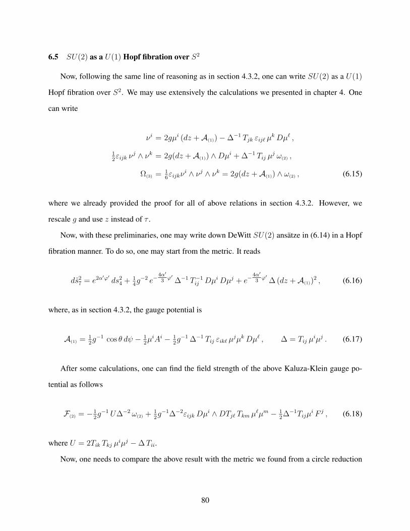
6.5 SU(2) as a U(1) Hopf fibration over S2
Now, following the same line of reasoning as in section 4.3.2, one can write SU(2) as a U(1)
Hopf fibration over S2. We may use extensively the calculations we presented in chapter 4. One
can write
νi = 2gµi (dz +A(1))−∆−1 Tjk εijℓ µkDµℓ ,
12εijk ν
j ∧ νk = 2g(dz +A(1)) ∧Dµi +∆−1 Tij µj ω(2) ,
Ω(3) =16εijkν
i ∧ νj ∧ νk = 2g(dz +A(1)) ∧ ω(2) , (6.15)
where we already provided the proof for all of above relations in section 4.3.2. However, we
rescale g and use z instead of τ .
Now, with these preliminaries, one may write down DeWitt SU(2) ansätze in (6.14) in a Hopf
fibration manner. To do so, one may start from the metric. It reads
ds27 = e2α′φ′ds24 +
14g−2 e−
4α′
3φ′∆−1 T−1
ij DµiDµj + e−4α′
3φ′∆(dz +A(1))
2 , (6.16)
where, as in section 4.3.2, the gauge potential is
A(1) =12g−1 cos θ dψ − 1
2µiAi − 1
2g−1∆−1 Tij εikℓ µ
jµkDµℓ , ∆ = Tij µiµj . (6.17)
After some calculations, one can find the field strength of the above Kaluza-Klein gauge po-
tential as follows
F(2) = −12g−1 U∆−2 ω(2) +
12g−1∆−2εijkDµ
i ∧DTjℓ Tkm µℓµm − 12∆−1Tijµ
i F j , (6.18)
where U = 2Tik Tkj µiµj −∆Tii.
Now, one needs to compare the above result with the metric we found from a circle reduction
80
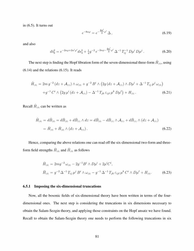
in (6.5). It turns out
e−8αφ = e−4α′
3φ′∆ , (6.19)
and also
ds26 = e−2αφ+2α′φ′ds24 +
14g−2 e−2αφ−4α′
3φ′∆−1 T−1
ij DµiDµj . (6.20)
The next step is finding the Hopf fibration form of the seven-dimensional three-form H(3), using
(6.14) and the relations (6.15). It reads
H(3) = 2mg−2 (dz +A(1)) ∧ ω(2) + g−2Bi ∧(2g (dz +A(1)) ∧Dµi +∆−1 Tij µ
j ω(2)
)+g−1Ci ∧
(2g µi (dz +A(1))−∆−1 Tjk εijℓ µ
kDµℓ)+H(3) . (6.21)
Recall H(3) can be written as
H(3) = dB(2) = dB(2) + dB(1) ∧ dz = dB(2) − dB(1) ∧ A(1) + dB(1) ∧ (dz +A(1))
= H(3) + H(2) ∧ (dz +A(1)) . (6.22)
Hence, comparing the above relations one can read off the six-dimensional two-form and three-
form field strengths H(2) and H(3) as follows
H(2) = 2mg−2 ω(2) − 2g−1Bi ∧Dµi + 2µiCi,
H(3) = g−2∆−1 Tij µj Bi ∧ ω(2) − g−1∆−1 Tjk εijℓ µ
k Ci ∧Dµℓ +H(3). (6.23)
6.5.1 Imposing the six-dimensional truncations
Now, all the bosonic fields of six-dimensional theory have been written in terms of the four-
dimensional ones. The next step is considering the truncations in six dimensions necessary to
obtain the Salam-Sezgin theory, and applying those constraints on the Hopf ansatz we have found.
Recall to obtain the Salam-Sezgin theory one needs to perform the following truncations in six
81
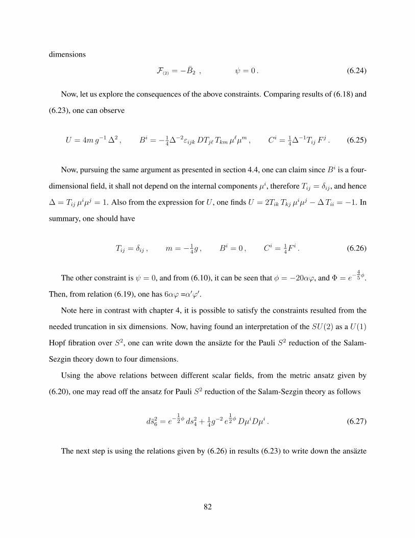
dimensions
F(2) = −B2 , ψ = 0 . (6.24)
Now, let us explore the consequences of the above constraints. Comparing results of (6.18) and
(6.23), one can observe
U = 4mg−1∆2 , Bi = −14∆−2εijkDTjℓ Tkm µ
ℓµm , C i = 14∆−1Tij F
j . (6.25)
Now, pursuing the same argument as presented in section 4.4, one can claim since Bi is a four-
dimensional field, it shall not depend on the internal components µi, therefore Tij = δij , and hence
∆ = Tij µiµj = 1. Also from the expression for U , one finds U = 2Tik Tkj µ
iµj −∆Tii = −1. In
summary, one should have
Tij = δij , m = −14g , Bi = 0 , C i = 1
4F i . (6.26)
The other constraint is ψ = 0, and from (6.10), it can be seen that ϕ = −20αφ, and Φ = e−45ϕ.
Then, from relation (6.19), one has 6αφ =α′φ′.
Note here in contrast with chapter 4, it is possible to satisfy the constraints resulted from the
needed truncation in six dimensions. Now, having found an interpretation of the SU(2) as a U(1)
Hopf fibration over S2, one can write down the ansäzte for the Pauli S2 reduction of the Salam-
Sezgin theory down to four dimensions.
Using the above relations between different scalar fields, from the metric ansatz given by
(6.20), one may read off the ansatz for Pauli S2 reduction of the Salam-Sezgin theory as follows
ds26 = e−12ϕ ds24 +
14g−2 e
12ϕDµiDµi . (6.27)
The next step is using the relations given by (6.26) in results (6.23) to write down the ansäzte
82
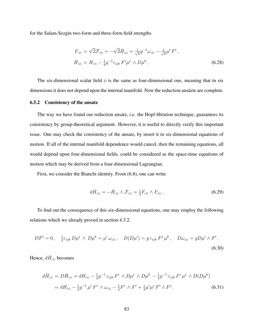
for the Salam-Sezgin two-form and three-form field strengths
F(2) =√2F(2) = −
√2H(2) =
1√2g−1ω(2) − 1√
2µi F i ,
H(3) = H(3) − 14g−1εijk F
iµj ∧Dµk . (6.28)
The six-dimensional scalar field ϕ is the same as four-dimensional one, meaning that in six
dimensions it does not depend upon the internal manifold. Now the reduction ansäzte are complete.
6.5.2 Consistency of the ansatz
The way we have found our reduction ansatz, i.e. the Hopf fibration technique, guarantees its
consistency by group-theoretical argument. However, it is useful to directly verify this important
issue. One may check the consistency of the ansatz, by insert it in six-dimensional equations of
motion. If all of the internal manifold dependence would cancel, then the remaining equations, all
would depend upon four-dimensional fields, could be considered as the space-time equations of
motion which may be derived from a four-dimensional Lagrangian.
First, we consider the Bianchi identity. From (6.8), one can write
dH(3) = −H(2) ∧ F(2) =12F(2) ∧ F(2) . (6.29)
To find out the consequence of this six-dimensional equations, one may employ the following
relations which we already proved in section 4.3.2.
DF i = 0 , 12εijkDµ
j ∧ Dµk = µi ω(2) , D(Dµi) = g εijk Fj µk , Dω(2) = gDµi ∧ F i .
(6.30)
Hence, dH(3) becomes
dH(3) = DH(3) = dH(3) − 14g−1 εijk F
i ∧Dµj ∧Dµk − 14g−1 εijk F
i µj ∧D(Dµk)
= dH(3) − 12g−1 µi F i ∧ ω(2) − 1
4F i ∧ F i + 1
4µiµj F i ∧ F j . (6.31)
83
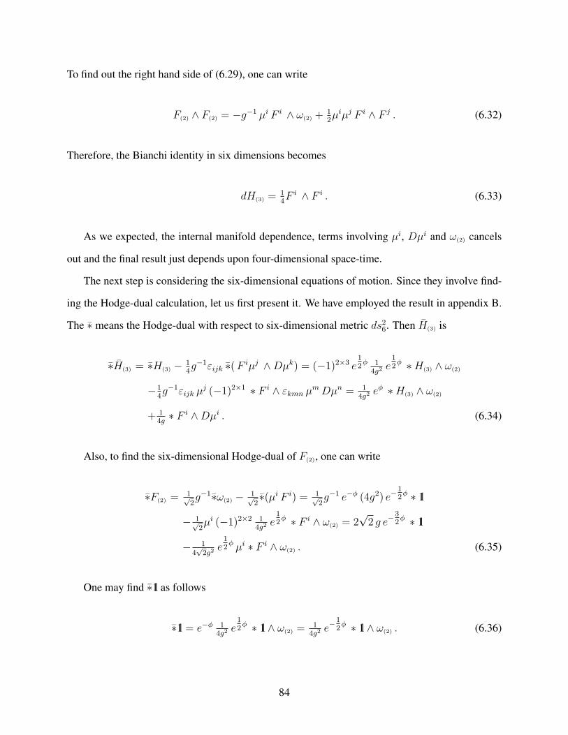
To find out the right hand side of (6.29), one can write
F(2) ∧ F(2) = −g−1 µi F i ∧ ω(2) +12µiµj F i ∧ F j . (6.32)
Therefore, the Bianchi identity in six dimensions becomes
dH(3) =14F i ∧ F i . (6.33)
As we expected, the internal manifold dependence, terms involving µi, Dµi and ω(2) cancels
out and the final result just depends upon four-dimensional space-time.
The next step is considering the six-dimensional equations of motion. Since they involve find-
ing the Hodge-dual calculation, let us first present it. We have employed the result in appendix B.
The ∗ means the Hodge-dual with respect to six-dimensional metric ds26. Then H(3) is
∗H(3) = ∗H(3) − 14g−1εijk ∗(F iµj ∧Dµk) = (−1)2×3 e
12ϕ 1
4g2e12ϕ ∗H(3) ∧ ω(2)
−14g−1εijk µ
j (−1)2×1 ∗ F i ∧ εkmn µmDµn = 14g2
eϕ ∗H(3) ∧ ω(2)
+ 14g
∗ F i ∧Dµi . (6.34)
Also, to find the six-dimensional Hodge-dual of F(2), one can write
∗F(2) =1√2g−1∗ω(2) − 1√
2∗(µi F i) = 1√
2g−1 e−ϕ (4g2) e−
12ϕ ∗ 1l
− 1√2µi (−1)2×2 1
4g2e12ϕ ∗ F i ∧ ω(2) = 2
√2 g e−
32ϕ ∗ 1l
− 14√2g2
e12ϕ µi ∗ F i ∧ ω(2) . (6.35)
One may find ∗1l as follows
∗1l = e−ϕ 14g2
e12ϕ ∗ 1l ∧ ω(2) =
14g2
e−12ϕ ∗ 1l ∧ ω(2) . (6.36)
84
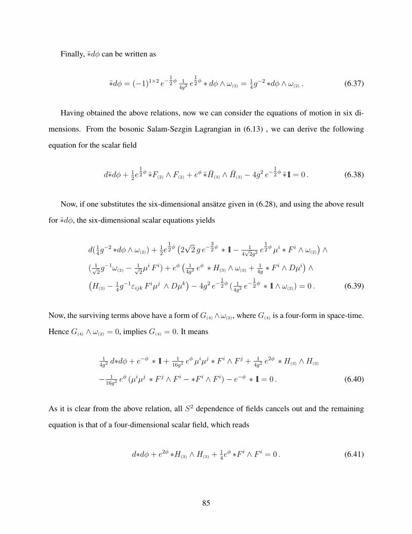
Finally, ∗dϕ can be written as
∗dϕ = (−1)1×2 e−12ϕ 1
4g2e12ϕ ∗ dϕ ∧ ω(2) =
14g−2 ∗dϕ ∧ ω(2) . (6.37)
Having obtained the above relations, now we can consider the equations of motion in six di-
mensions. From the bosonic Salam-Sezgin Lagrangian in (6.13) , we can derive the following
equation for the scalar field
d∗dϕ+ 12e12ϕ ∗F(2) ∧ F(2) + eϕ ∗H(3) ∧ H(3) − 4g2 e−
12ϕ ∗1l = 0 . (6.38)
Now, if one substitutes the six-dimensional ansätze given in (6.28), and using the above result
for ∗dϕ, the six-dimensional scalar equations yields
d(14g−2 ∗dϕ ∧ ω(2)) +
12e12ϕ(2√2 g e−
32ϕ ∗ 1l− 1
4√2g2
e12ϕ µi ∗ F i ∧ ω(2)
)∧
( 1√2g−1ω(2) − 1√
2µi F i) + eϕ
(1
4g2eϕ ∗H(3) ∧ ω(2) +
14g
∗ F i ∧Dµi)∧(
H(3) − 14g−1εijk F
iµj ∧Dµk)− 4g2 e−
12ϕ ( 1
4g2e−
12ϕ ∗ 1l ∧ ω(2)) = 0 . (6.39)
Now, the surviving terms above have a form of G(4) ∧ω(2), where G(4) is a four-form in space-time.
Hence G(4) ∧ ω(2) = 0, implies G(4) = 0. It means
14g2
d∗dϕ+ e−ϕ ∗ 1l + 116g2
eϕ µiµj ∗ F i ∧ F j + 14g2
e2ϕ ∗H(3) ∧H(3)
− 116g2
eϕ (µiµj ∗ F j ∧ F i − ∗F i ∧ F i)− e−ϕ ∗ 1l = 0 . (6.40)
As it is clear from the above relation, all S2 dependence of fields cancels out and the remaining
equation is that of a four-dimensional scalar field, which reads
d∗dϕ+ e2ϕ ∗H(3) ∧H(3) +14eϕ ∗F i ∧ F i = 0 . (6.41)
85
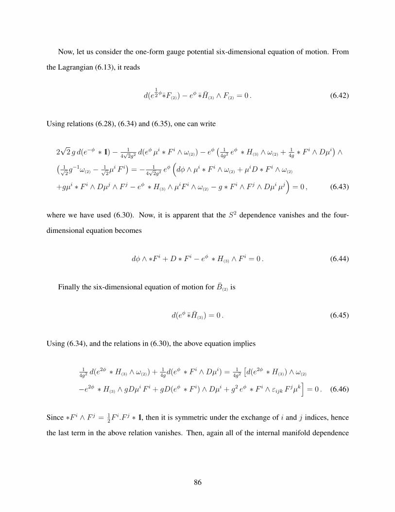
Now, let us consider the one-form gauge potential six-dimensional equation of motion. From
the Lagrangian (6.13), it reads
d(e12ϕ∗F(2))− eϕ ∗H(3) ∧ F(2) = 0 . (6.42)
Using relations (6.28), (6.34) and (6.35), one can write
2√2 g d(e−ϕ ∗ 1l)− 1
4√2g2
d(eϕ µi ∗ F i ∧ ω(2))− eϕ(
14g2
eϕ ∗H(3) ∧ ω(2) +14g
∗ F i ∧Dµi)∧(
1√2g−1ω(2) − 1√
2µi F i
)= − 1
4√2g2
eϕ(dϕ ∧ µi ∗ F i ∧ ω(2) + µiD ∗ F i ∧ ω(2)
+gµi ∗ F i ∧Dµj ∧ F j − eϕ ∗H(3) ∧ µiF i ∧ ω(2) − g ∗ F i ∧ F j ∧Dµi µj)= 0 , (6.43)
where we have used (6.30). Now, it is apparent that the S2 dependence vanishes and the four-
dimensional equation becomes
dϕ ∧ ∗F i +D ∗ F i − eϕ ∗H(3) ∧ F i = 0 . (6.44)
Finally the six-dimensional equation of motion for B(2) is
d(eϕ ∗H(3)) = 0 . (6.45)
Using (6.34), and the relations in (6.30), the above equation implies
14g2
d(e2ϕ ∗H(3) ∧ ω(2)) +14gd(eϕ ∗ F i ∧Dµi) = 1
4g2
[d(e2ϕ ∗H(3)) ∧ ω(2)
−e2ϕ ∗H(3) ∧ gDµi F i + gD(eϕ ∗ F i) ∧Dµi + g2 eϕ ∗ F i ∧ εijk F jµk]= 0 . (6.46)
Since ∗F i ∧ F j = 12F i.F j ∗ 1l, then it is symmetric under the exchange of i and j indices, hence
the last term in the above relation vanishes. Then, again all of the internal manifold dependence
86
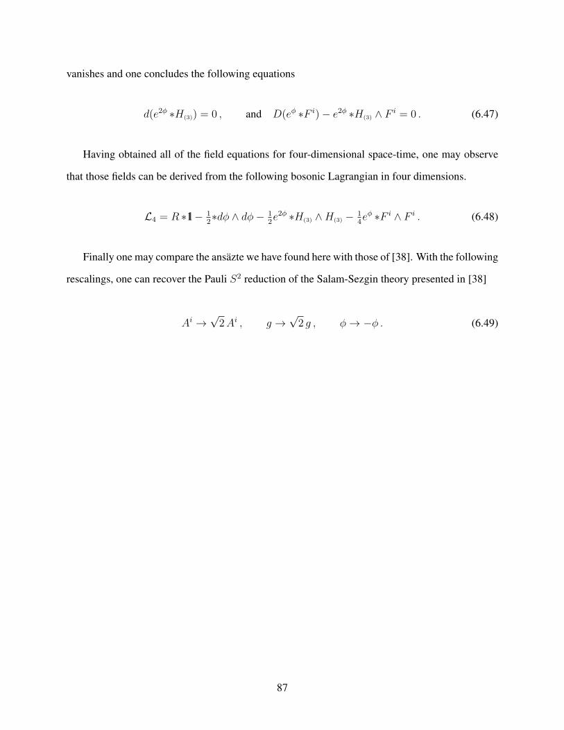
vanishes and one concludes the following equations
d(e2ϕ ∗H(3)) = 0 , and D(eϕ ∗F i)− e2ϕ ∗H(3) ∧ F i = 0 . (6.47)
Having obtained all of the field equations for four-dimensional space-time, one may observe
that those fields can be derived from the following bosonic Lagrangian in four dimensions.
L4 = R ∗1l− 12∗dϕ ∧ dϕ− 1
2e2ϕ ∗H(3) ∧H(3) − 1
4eϕ ∗F i ∧ F i . (6.48)
Finally one may compare the ansäzte we have found here with those of [38]. With the following
rescalings, one can recover the Pauli S2 reduction of the Salam-Sezgin theory presented in [38]
Ai →√2Ai , g →
√2 g , ϕ→ −ϕ . (6.49)
87
7. CONCLUSION AND OUTLOOK
In this dissertation, we have investigated different consistent Kaluza-Klein-Pauli reductions.
All the dimensional reductions we have considered are Pauli (coset) reductions, which besides few
exceptions, they are generally inconsistent.
In chapter 2, we considered a toy example of the Klein-Gordon scalar field, and explaining why
one has an infinite massive tower of fields in the lower dimensional theory, after a circle reduction
of a massless scalar in the higher dimensions. Also, we presented the reduction ansätze for the
metric and gauge potential for the circle reduction.
In chapter 3, we found the embedding of two specific truncations, i.e. 3 + 1 and 2 + 2 of STU
gauge supergravity, in eleven dimensions. STU gauged supergravity is a maximal Abelian sub-
group of the eminent N = 8, gauged SO(8) four-dimensional supergravity. We have found the
metric and four-form field strength ansätze for 3 + 1 case for the first time, and we could recover
the results of [34] in 2 + 2 truncation.
We have used a systematic method to find Pauli reductions. This method was introduced in [7]
and named “Hopf fibration technique” in [45]. One performs a consistent DeWitt reduction of a
higher dimensional initial theory, say T1, on a group manifold G down to the lower-dimensional
space-time theory, named T3. Furthermore, one may construct another consistent DeWitt reduction
of T1 on a group manifold H , where G ⊃ H , and obtains a theory T2 whose dimension is higher
than that of the space-time. The claim is, there is a consistent Pauli reduction of T2 on a coset space
G/H to give the space-time theory, T3. It can be justified, if one considers a Hopf fibration of G
as a group manifold H bundle over a coset space G/H , then the consistency of the Pauli reduction
on a coset space G/H is guaranteed based on the consistencies of both DeWitt reductions of T1
on group manifolds G and H . Thanks to this Hopf fibration technique, one may find out a deeper
understanding of why a “miraculous” Pauli reduction works.
We have employed the Hopf fibration technique to investigate the possibility of the Pauli re-
ductions in two different scenarios. First, in chapter 4, we consider an S2 reduction of the minimal
88
supergravity in five dimensions. The main motivation for this investigation is the resemblance
of the bosonic Lagrangian of the latter theory and that of eleven-dimensional supergravity. As a
result of this analogy, and since there are S7, S4 and S5 Pauli reductions of eleven-dimensional
supergravity, one may conjecture there are S2 or S3 reductions of minimal supergravity in five
dimensions. Making use of this technique, one may start from minimal supergravity in six di-
mensions as the initial theory, and perform an S1 reduction to find minimal supergravity coupled
to a vector multiplet in five dimensions. However, to obtain pure five-dimensional minimal su-
pergravity, one needs to perform consistent truncations in five dimensions. The next step, shall
be an SU(2) DeWitt reduction of the initial theory to give a three-dimensional space-time. Now,
viewing the S3 = SU(2) as a Hopf fibration of an S1 bundle over coset space S2 = S3/S1, one
can find the consistent Pauli S2 reduction of the five-dimensional minimal supergravity coupled
to a vector multiplet. While it is an interesting result in its own right, this construction has not
been our main goal of the investigation, and we are looking to find an S2 reduction of pure five-
dimensional minimal supergravity. As we have mentioned above, one needs to perform truncations
in five dimensions to obtain the latter theory from the former one. However, a simple consideration
shows these truncations are not compatible with the ansatz we have found for minimal supergrav-
ity coupled to a vector multiplet, and the search for constructing the Pauli reduction of minimal
supergravity fails. Although this analysis does not provide a rigorous mathematical proof of the
impossibility of the reduction, it is very promising. Especially, we have tried to find a trial ansatz
and by inspecting the higher dimensional equations of motion, we hoped to find the correct ansatz.
Again, this method failed to give a correct ansatz. Therefore, by considering these examinations,
it seems very persuading to believe there is no consistent Pauli S2 of the minimal supergravity in
five dimensions.
Our second inquiry, in chapter 6 is revisiting an interesting question of the possibility of a
consistent S2 Pauli reduction of six-dimensional N = (1, 0) Einstein-Maxwell supergravity. The
latter theory found by Salam and Sezgin in 1984, and hence it has been named Salam-Sezgin
theory. Since this theory admits a Minkowski4 × S2 vacuum with N = 1 supersymmetry, it is
89
an interesting inquiry to find out whether this theory admits the full non-linear Pauli S2 reduction.
Gibbons and Pope found out a “remarkable” consistent reduction ansatz in 2003, however, the
underlying reason of why this ansatz is achievable remains obscure. Furthermore, Salam and
Sezgin observed in their original paper [36], since the integer S2 Dirac monopole charge n has
been fixed by the equations of motion to be n = ±1, then regarding the fact that an S2 with a
singly charge Dirac monopole on it is an S3, they conjectured the possibility of the presence of an
S3 dimensional reduction of a seven-dimensional theory to give the four-dimensional Minkowski
vacuum they found from the spontaneous compactification of their theory. This is exactly what we
have found with the Hopf fibration technique.
To use the Hopf fibration technique, one needs to find an embedding of the Salam-Sezgin
theory in a higher-dimensional one. This has been done in [39] and an M-theory origin of this
theory has been found. However, the Kaluza vector potential A(1), arises from a circle reduction
of the metric of a seven-dimensional theory, was set to zero in their work. Since this vector field
is corresponding to a Dirac monopole on S2, its vanishing means the monopole charge has to be
set to zero, and hence the resulting Hopf fibration is just a trivial S2 × S1 instead of the expected
S3 one. To remedy this problem, one has to find another embedding of the Salam-Sezgin theory
where the vector potential A(1) is non-zero. We have found such an embedding.
The alternative embedding of the Salam-Sezgin theory in M-theory has been found based on
the assumption that the Kaluza vector potential A(1) is not zero. The striking feature of this embed-
ding is the role of a constant axion. According to the standard Kaluza-Klein circle reduction, one
may obtain a scalar, named axion, from a reduction of a vector one-form gauge potential. While
this axion has been always assumed either to be truncated to zero or to be a scalar field depends
on the space-time coordinate in the literature, we presume this field is a constant to be determined
by the supersymmetry transformations. By this premise, one can retain the usual covariant deriva-
tive. Since the six-dimensional Yang-Mills gauge potentials are truncated to zero in our scheme,
one needs a vector potential in the covariant derivative to be gauged. Thanks to the circle reduc-
tion, the Kaluza vector potential A(1) appears along with an axion in the covariant derivative of
90
six-dimensional theory, and this vector potential can play a role of the usual gauge vector in the
covariant derivative as a result of the constant axion.
In the first embedding of the Salam-Sezgin theory in M-theory found in [39], it was assumed
the compact SO(4) gauge group of the seven-dimensional theory is changed to a non-compact
group of SO(2, 2). They could recover the positive definite potential of the Salam-Sezgin theory
by this premise. We constructed the alternative embedding, in the bosonic sector, with the non-
compact gauging in chapter 6, where the vector potential A(1) is non-zero. However, to retain the
vector potential A(1), if one would consider the fermionic sector as well, one has to start from
an N = 2 with SO(4) gauging, but a ‘Wick rotated’ supergravity in seven dimensions, as it was
shown in chapter 5. The Wick rotation can be achieved by either δAB → −i δAB or Φ1/4 →
−i Φ1/4, together with HMNP → −HMNP . However, as we have emphasized in chapter 5, the
reality condition of this theory is not very clear. This is why we did not present our fermionic
calculation in this dissertation. Nevertheless, both supersymmetry transformations maintain the
Lagrangian is invariant under them. More promising, we could find exactly the same Lagrangian,
both bosonic and fermionic sectors, as that of the Salam-Sezgin theory. Also, according to our
fermionic truncations, the supersymmetry transformations become the same as those of the Salam-
Sezgin theory.
Upon writing down the embedding of seven-dimensional metric ansatz in ten dimensions, one
can observe that the Wick rotated theory in seven dimensions, results from a time-like reduction of
ten-dimensional type I theory. In other words, the metric of the internal manifold, has an overall
negative sign as opposed to the usual positive sign. Time-like reduction is an interesting possibility
in the dimensional reduction program, which explored by Hull in 1990s [50, 51]. Since reduction
is time-like, then the higher dimensional theory should have a different space-time signature than
that of Minkowski. In this case, to obtain a (t, s) = (1, 6) theory with three time-like compact
coordinates, the ten dimensional theory should have a signature of (t, s) = (4, 6). This is a possi-
bility in Hull’s work in [50] as a type IIA (4,6). It is intriguing that the Salam-Sezgin theory has
an embedding with the usual space-like reduction and also an exotic time-like one.
91
Having found an alternative embedding of the Salam-Sezgin theory with non-zero vector po-
tential A(1), one can follow the Hopf fibration technique to find an S2 reduction of the latter theory.
In chapter 6, we showed in detail how this works. After performing a circle reduction of seven-
dimensional theory, one needs to impose a truncation to obtain the Salam-Sezgin theory in six
dimensions. The crucial point is to verify whether this truncation is consistent with the Hopf
ansatz we find. Unlike the case of chapter 4, we showed this truncation is actually consistent with
the Hopf ansatz in chapter 6, meaning that, there is a consistent Pauli S2 reduction of the Salam-
Sezgin theory down to four dimensions. The two contrasting examples of chapters 4 and 6 show
how a truncation can be critical for the possibility of finding a consistent Pauli reduction.
One may employ the Hopf reduction technique to find more Pauli reductions of different su-
pergravities. Especially the case of Pauli S2 reduction is the easiest one to implement. However,
one may consider more involved geometries and may find more interesting Pauli reductions. In
addition to this, one may use the assumption of the constant axion to find different truncations,
especially when there is a Maxwell gauge potential in the higher-dimensional theory. Since one
may truncate the lower-dimensional Maxwell gauge potential to zero and by keeping the axion as a
constant number, one can still retain the usual gauging in the lower-dimensional theory by making
use of the Kaluza-Klein vector potential.
The other exciting possibility is the time-like reduction which may give rise to more consistent
dimensional reductions or even constructing of unknown supergravities.
92
REFERENCES
[1] G. Nordström, Über die Möglichkeit, das elektromagnetische Feld und das Gravitationsfeld
zu vereinigen, Phys. Zeitschr. 15 (1914) 504.
[2] L. O’Raifeartaigh and N. Straumann, Early history of gauge theories and Kaluza-Klein the-
ories, with a glance at recent developments, [arXiv: 9810524 [hep-th]].
[3] Th. Kaluza, Zum Unitätsproblem der Physik , Sitzunber. Preuss. Akad. Wiss. Berlin. Math.
Phys. K1 (1921) 966 ; for an English translation see Ref. [8].
[4] O. Klein, Quantentheorie und fünfdimensionale Relativitätstheorie, Z. Phys. 37 895 (1926);
for an English translation see Ref. [8].
[5] M.J. Duff, B.E.W. Nilsson, C.N. Pope and N.P. Warner, On the consistency of the Kaluza-
Klein ansatz, Phys. Lett. B149 (1984) 90.
[6] B.S. DeWitt, in Relativity, groups and topology, Les Houches 1963 (Gordon and Breach,
1964).
[7] M. Cvetic, G.W. Gibbons, H. Lü and C.N. Pope, Consistent group and coset reductions of
the bosonic string, Class. Quant. Grav. 20 (2003) 5161 [arXiv: 0306043 [hep-th]].
[8] W. Pauli, Wissenschaftlicher Briefwechsel, Vol. I: 1919-1929. p. 505, Springer-Verlag 1979.
(Translation of the letter by L. O’Raifeartaigh.)
[9] N. Straumann, On Pauli’s invention of non-Abelian Kaluza-Klein theory in 1953, [arXiv:
0012054 [gr-qc]].
[10] B. de Wit and H. Nicolai, N = 8 supergravity, Nucl.Phys. B208 (1982) 323.
[11] B. de Wit and H. Nicolai, The consistency of the S7 truncation in D = 11 supergravity, Nucl.
Phys. B281 (1987) 211.
[12] B. de Wit and H. Nicolai, Deformations of gauged SO(8) supergravity and supergravity in
eleven dimensions, JHEP 1305 (2013) 077 [arXiv: 1302.6219 [hep-th]].
93
[13] H. Nastase, D. Vaman and P. van Nieuwenhuizen, Consistent nonlinear KK reduction of 11-d
supergravity on AdS7 × S4 and selfduality in odd dimensions, Phys. Lett. B469 (1999) 96
[arXiv: 9905075 [hep-th]].
[14] H. Nastase, D. Vaman and P. van Nieuwenhuizen, Consistency of the AdS7×S4 reduction and
the origin of self-duality in odd dimensions, Nucl. Phys. B581 (2000) 179 [arXiv: 9911238
[hep-th]].
[15] M. Cvetic, H. Lü, C.N. Pope, A. Sadrzadeh and T.A. Tran, S3 and S4 reductions of type IIA
supergravity, Nucl. Phys. B590 (2000) 233 [arXiv: 0005137 [hep-th]].
[16] A. Baguet, O. Hohm and H. Samtleben, Consistent type IIB reductions to maximal 5D super-
gravity, Phys. Rev. D92 no. 6 (2015) 065004 [arXiv: 1506.01385 [hep-th]].
[17] A. Baguet, C.N. Pope and H. Samtleben, Consistent Pauli reduction on group manifolds,
Phys. Lett. B752 (2016) 278 [arXiv: 1510.08926 [hep-th]].
[18] E. Witten, Search for a Realistic Kaluza-Klein Theory, Nucl. Phys. B186 (1981) 412.
[19] J. Scherk and J. Schwarz, How to Get Masses from Extra Dimensions, Nucl. Phys. B153
(1979) 61.
[20] M.J. Duff and C.N. Pope, Kaluza-Klein supergravity and the seven-sphere, pp. 183228. World
Scientific, 1983.
[21] M.J. Duff, B.E.W. Nilsson and C.N. Pope, Kaluza-Klein Supergravity, Phys. Rept. 130 (1986)
1.
[22] B. Biran, F. Englert, B. de Wit, and H. Nicolai, Gauged N = 8 supergravity and its breaking
from spontaneous compactification, Phys. Lett. B124 (1983) 45. [Erratum: Phys. Lett. B128,
(1983) 461].
[23] J.M. Maldacena, The large N limit of superconformal field theories and supergravity, Adv.
Theor. Math. Phys. 2 (1998) 231 [Int. J. Theor. Phys. 38 (1999) 1113] [arXiv: 9711200 [hep-
th]].
94
[24] E. Witten, Anti-de Sitter space and holography, Adv. Theor. Math. Phys. 2 (1998) 253 [arXiv:
9802150 [hep-th]].
[25] S.S. Gubser, I.R. Klebanov and A.M. Polyakov, Gauge theory correlators from non-critical
string theory, Phys. Lett. B 428 (1998) 105 [arXiv: 9802109 [hep-th]].
[26] C.N. Pope, Kaluza-Klein Theory, http://people.physics.tamu.edu/pope/ihplec.pdf.
[27] M. Cvetic, H. Lü, C.N. Pope, A. Sadrzadeh and T.A. Tran, Consistent SO(6) reduction of
type IIB supergravity on S5, Nucl. Phys. B586 (2000) 275 [arXiv: 0003103 [hep-th]].
[28] M. Cvetic, H. Lü and C.N. Pope, Gauged six-dimensional supergravity from massive type
IIA, Phys. Rev. Lett. 83 (1999) 5226 [arXiv: 9906221 [hep-th]].
[29] M. Cvetic, H. Lü and C.N. Pope, Consistent Kaluza-Klein sphere reductions, Phys. Rev. D62
(2000) 064028 [arXiv: 0003286 [hep-th]].
[30] M.J. Duff, B.E.W. Nilsson, C.N. Pope and N.P. Warner, Kaluza-Klein approach to the het-
erotic string. 2, Phys. Lett. B171 (1986) 170.
[31] O. Hohm, C. Hull and B. Zwiebach, Generalized metric formulation of double field theory,
JHEP 1008 (2010) 008 [arXiv: 1006.4823 [hep-th]].
[32] O. Hohm and H. Samtleben, Exceptional Form of D=11 Supergravity, Phys. Rev. Lett. 111
(2013) 231601 [arXiv: 1308.1673 [hep-th]].
[33] A. Azizi, H. Godazgar, M. Godazgar, and C. N. Pope, Embedding of gauged STU supergrav-
ity in eleven dimensions, Phys. Rev. D94 no. 6 (2016) 066003 [arXiv: 1606.06954 [hep-th]].
[34] M. Cvetic, H. Lü, and C.N. Pope, Four-dimensional N = 4, SO(4) gauged supergravity
from D = 11, Nucl. Phys. B574 (2000) 761 [arXiv: 9910252 [hep-th]].
[35] M. Cvetic, H. Lü, and C.N. Pope, Geometry of the embedding of supergravity scalar mani-
folds in D = 11 and D = 10, Nucl. Phys. B584 (2000) 149 [arXiv: 0002099 [hep-th]].
[36] A. Salam and E. Sezgin, Chiral compactification on (Minkowski)×S2 of N = 2 Einstein-
Maxwell supergravity in six-dimensions, Phys. Lett. B147 (1984) 47.
95
[37] H. Nishino and E. Sezgin, Matter and gauge couplings of N=2 supergravity in six dimensions,
Phys. Lett. B144 (1984) 187.
[38] G.W. Gibbons and C.N. Pope, Consistent S2 Pauli reduction of six-dimensional chiral gauged
Einstein-Maxwell supergravity, Nucl. Phys. B697 (2004) 225 [arXiv: 0307052 [hep-th]].
[39] M. Cvetic, G.W. Gibbons and C.N. Pope, A string and M-theory origin for the Salam-Sezgin
model, Nucl. Phys. B677 (2004) 164 [arXiv: 0308026 [hep-th]].
[40] M. Pernici, K. Pilch, P. van Nieuwenhuizen, Gauged maximally extended supergravity in
seven dimensions, Phys. Lett. B143 (1984) 103.
[41] M. Pernici, K. Pilch, P. van Nieuwenhuizen and N. P. Warner, Noncompact gaugings and
critical points of maximal supergravity in seven-dimensions, Nucl. Phys. B249 (1985) 381.
[42] J.T. Liu and R. Minasian, Black holes and membranes in AdS7, Phys. Lett. B457 (1999) 39
[arXiv: 9903269 [hep-th]].
[43] J.M. Maldacena and C. Nunez, Supergravity description of field theories on curved manifolds
and a no go theorem , Int. J. Mod. Phys. A16 (2001) 822 [arXiv: 0007018 [hep-th]].
[44] H. Lü, C.N. Pope and E. Sezgin, SU(2) reduction of six-dimensional (1, 0) supergravity,
Nucl. Phys. B668 (2003) 237 [arXiv: 0212323 [hep-th]].
[45] A. Azizi and C.N. Pope, On Pauli reductions of supergravities in six and five dimensions,
[arXiv: 1802.07308 [hep-th]].
[46] P.K. Townsend and P. van Nieuwenhuizen, Gauged Seven-dimensional Supergravity, Phys.
Lett. B125 (1983) 41.
[47] H. Lu and C.N. Pope, Exact embedding of N=1, D = 7 gauged supergravity in D = 11, Phys.
Lett. B467 (1999) 67 [arXiv: 9906168 [hep-th]].
[48] C.N. Pope, T.G. Pugh and K.S. Stelle, Chiral Reductions in the Salam-Sezgin Model, JHEP
1202 (2012) 098 [arXiv:1108.6011 [hep-th]].
96
[49] M. Cvetic, M.J. Duff, P. Hoxha, J.T. Liu, H. Lü, J.X. Lu, R. Martinez-Acosta, C.N. Pope, H.
Sati and T.A. Tran, Embedding AdS black holes in ten and eleven dimensions, Nucl. Phys.
B558 (1999) 96 [arXiv: 9903214 [hep-th]].
[50] C.M. Hull, Duality and the signature of space-time, JHEP 9811 (1998) 017 [arXiv: 9807127
[hep-th]].
[51] C.M. Hull, Timelike T duality, de Sitter space, large N gauge theories and topological field
theory, JHEP 9807 (1998) 021 [arXiv: 9806146 [hep-th]].
97
APPENDIX A
FINDING THE FIELD RE-DEFINITIONS
It is important to find the field re-definitions between [36], the original paper of Salam and Sez-
gin, [40] where SO(5) gauged maximal supergravity in seven dimensions was initially constructed,
and [39] where the first embedding of the Salam-Sezgin theory was introduced. Especially since
the fermionic Lagrangian was not presented (beside the two kinetic terms) in the last work, one
needs to find the field re-definitions to obtain the the full fermionic Lagrangian of the Salam-Sezgin
theory, from reduction and truncations of the original theory of [40] and compare it with that of
the Salam and Sezgin work in [36].
Let us label fields and coupling constant of [36] and [40] with tilde and prime respectively,
while those of [39] are without any labeling. To begin with, one may compare the bosonic La-
grangian of SO(5) gauged maximal supergravity in seven dimensions, i.e. eqn (8) of [40] and eqn
(1) of [39]. Hence one can find the following
L7 = 2L′7, g = 1
2g′, F(2) =
√2F ′
(2), S(3) = −2√3 i mS ′
(3), (A.1)
where m = 12g′ in the former paper. One can observe that the supersymmetry transformations, eqn
(9) of [40] and equations (6) and (9) of [39], agree with each other upon considering the above field
redefinitions. However, there is a typographical error in eqn (2) of [39], where the field strength
was defined. According to [40] (below eqn (9)), the field strength was defined as usual
F ′(2)A
B = dA′(1)A
B + g′A′(1)A
C ∧ A′(1)C
B , (A.2)
where we rewrite it in the form-language, and also rename the vector potential from B(1) to A′(1).
98
Upon using the above field redefinitions, one has to find the following relation in [39]
F(2)AB = dA(1)A
B +√2 g A(1)A
C ∧ A(1)CB , (A.3)
where√2 is missing in eqn (2) of [39]. However, since we consider the abelian truncation of the
original theory to obtain the Salam-Sezgin theory, this issue shall be irrelevant. However, this issue
reflects in the definition of Qij . If one accepts the definition of this quantity as it is presented in
eqn (6) of [40], then Qij defined in eqn (2) of [39] should be modifies as follows
Π−1iA (δA
B d+√2 g A(1)A
B)ΠBk δkj = Pij +Qij ; Pij = P(ij) , Qij = Q[ij], (A.4)
where factor of√2 has been added. Since it is somewhat inconvenient to have the factor of
√2,
we redefine the gauge potential in the way that this factor becomes absorbed in that field. This is
the convention which used in [15] and we follow it.
99
APPENDIX B
FINDING THE HODGE-DUALITY RELATION WITH A SPHERICAL CONSTRAINT
B.1 The notation
We follow the convention and notion of [26]. For convenience, we present the main definitions
here. First of all, to specify our notation, consider a general p-form in a general D dimensions
ω(p) =1p!ωµ1µ2···µp dx
µ1 ∧ dxµ2 ∧ · · · ∧ dxµp . (B.1)
Then, the Hodge-dual of this p-form field is defined as follows
∗ (dxµ1 ∧ · · · ∧ dxµp) = 1q!ϵν1···νq
µ1···µp dxν1 ∧ · · · ∧ dxνq , (B.2)
where q = D − p. Here
ϵµ1···µD =√
|g| εµ1···µD (B.3)
is a totally anti-symmetric Levi-Civita tensor while the Levi-Civita tensor density εµ1···µD = (1,−1, 0)
for an even, odd or no permutation of (0, 1, · · · , D − 1) respectively. All upstairs indices Levi-
Civita density tensor is related to the above one as follows
εµ1···µD = (−1)t εµ1···µD , (B.4)
where t is number of time-like component in the metric. Here, since the Levi-Civita density tensor
is not a tensor, hence its indices do not raise and lower by the metric. However those of the
Levi-Civita tensor do raise and lower by the metric, then one can find out
ϵµ1···µD = 1√|g|εµ1···µD . (B.5)
100
One can use (B.2) to find the following relation for the components of a Hodge-dual form field
(∗ω)(q) ≡ 1q!(∗ω)ν1···νq dxν1 ∧ · · · ∧ dxνq ,
(∗ω)ν1···νq = 1p!ϵν1···νq
µ1···µp ωµ1···µp . (B.6)
Also, again using (B.2) for the case of p = 0, one can write
∗ 1l = 1D!ϵµ1···µD dx
µ1 ∧ · · · ∧ dxµD . (B.7)
Other important relation which we have been used it extensively is the applying the Hodge-dual
twice on a general p-form. The result is as follows
∗ ∗ ω(p) =1p!ωµ1···µp ∗ ∗(dxµ1 ∧ · · · ∧ dxµp) = 1
p!q!ωµ1···µp ϵν1···νq
µ1···µp ∗ (dxν1 ∧ · · · ∧ dxνq)
= 1p!q!
ωµ1···µp ϵν1···νqµ1···µp ϵρ1···ρp
ν1···νq dxρ1 ∧ · · · ∧ dxρp
= (−1)pq+t ωµ1···µp δµ1···µpρ1···ρp dx
ρ1 ∧ · · · ∧ dxρp = (−1)pq+t ωµ1···µp dxρ1 ∧ · · · ∧ dxρp
= (−1)pq+t ω(p), (B.8)
where δµ1···µpρ1···ρp = δ[µ1[ρ1
· · · δµp]ρp]. We have employed the following relation
ϵµ1···µpν1···νq ϵµ1···µpρ1···ρq = p!q! (−1)t δρ1···ρqν1···νq . (B.9)
Note according to the above definition one has δµ1···µDµ1···µD = 1.
Another useful relation is ∗A(p) ∧B(p) =1p!A.B ∗ 1l. The proof is as follows
∗A(p) ∧B(p) =1
p!2q!Aµ1···µp ϵν1···νq
µ1···µp Bρ1···ρp dxν1 ∧ · · · ∧ dxνq ∧ dxρ1 ∧ · · · ∧ dxρp
= 1p!2q!
Aµ1···µp Bρ1···ρp ϵν1···νqµ1···µp(−1)t ϵν1···νqρ1···ρp ∗ 1l (B.10)
= 1p!δρ1···ρpµ1···µp A
µ1···µp Bρ1···ρp ∗ 1l = 1p!Aµ1···µp Bµ1···µp ∗ 1l = 1
p!A.B ∗ 1l ,
101
where we have used (B.9) and also
dxµ1 ∧ · · · ∧ dxµD = (−1)t ϵµ1···µD ∗ 1l , (B.11)
where one can readily find out this relation from (B.7).
B.2 The Hodge-dual on a sphere
In this section, we consider an important problem of finding the Hodge-dual of a general p-
form on a sphere. For simplicity one can assume the sphere has a unit radius. Then, one may
parametrize the (D− 1)-sphere in D dimensions by xµ where δµνxµxν = 1. Note that the index in
xµ can raise and lower by the delta Dirac metric and hence one may simply write the constraint as
xµxµ = 1. Then considering the following metric
ds2 = gµν dxµdxν , (B.12)
one needs to find the following Hodge-dual ∗(dxµ1 ∧ · · · ∧ dxµp). Because of the constraint, D− 1
components are independent, and hence the Hodge-dual of a p-form shall be a D − p− 1 = q − 1
form. Considering this point, the most general form of the Hodge-dual of a p-form is as follows
∗ (dxµ1 ∧ · · · ∧ dxµp) = 1(q−1)!
ϵνν1···νq−1
µ1···µp Aν dxν1 ∧ · · · ∧ dxνq−1 , (B.13)
102

when Aν is a general function to be determined. To find this function, one may apply the Hodge-
dual operation twice on a p-form as follows
∗ ∗ (dxµ1 ∧ · · · ∧ dxµp) = 1(q−1)!
ϵνν1···νq−1
µ1···µp Aν ∗ (dxν1 ∧ · · · ∧ dxνq−1)
= 1p!(q−1)!
ϵνν1···νq−1
µ1···µp Aν ϵρρ1···ρpν1···νq−1 Aρ dxρ1 ∧ · · · ∧ dxρp
= (−1)p(q−1)
p!(q−1)!ϵνµ1···µpν1···νq−1 Aν ϵρρ1···ρp
ν1···νq−1 Aρ dxρ1 ∧ · · · ∧ dxρp
= (p+ 1) (−1)p(q−1)+t δνµ1···µpρρ1···ρp Aν Aρ dxρ1 ∧ · · · ∧ dxρp
= (−1)p(q−1)+t (δνρ δµ1···µpρ1···ρp − p δνρ1 δ
µ1···µpρ···ρp )Aν A
ρ dxρ1 ∧ · · · ∧ dxρp
= (−1)p(q−1)+t(Aν A
ν dxµ1 ∧ · · · ∧ dxµp − pAν dxν Aµ1 ∧ · · · ∧ dxµp
)= (−1)p(q−1)+t dxµ1 ∧ · · · ∧ dxµp , (B.14)
where we have used (p + 1) δνµ1···µpρρ1···ρp = δνρ δ
µ1···µpρ1···ρp − p δν[ρ1 δ
µ1···µp|ρ|···ρp], and the anti-symmetrization has
been dropped since this term is coupled to dxρ1 ∧ · · ·∧dxρp . The last line was written according to
the general result of (B.8). To achieve this result, the following two conditions should be satisfied
Aν Aν = 1 , Aν dx
ν = 0 . (B.15)
We claim the following expression for Aµ will fulfill both of the above conditions
Aµ = 1√∆gµν xν , (B.16)
where ∆ = gµν xµxν . Now, one may readily check the above expression satisfies both conditions
in (B.15) as follows
Aµ dxµ = gµν A
µdxν = 1√∆gµν g
µρ xρ dxν = 1√∆xν dxν = 1
2√∆d(xν xν) = 0 ,
AµAµ = gµν A
µAν = 1∆gµν g
µρxρ gνσxσ = 1∆gνσ xνxσ = 1 . (B.17)
103
This completes the proof. Thus the final result for a Hodge-dual of a general p-form with the
constraint of xµxµ = 1 shall be
∗ (dxµ1 ∧ · · · ∧ dxµp) = 1(q−1)!
1√∆ϵνν1···νq−1
µ1···µp gνρ xρ dxν1 ∧ · · · ∧ dxνq−1 . (B.18)
One can may consider two important special cases of the above general result.
Corollary 1. Consider the case p = 0. Then we have
∗1l = 1(D−1)!
1√∆ϵνν1···νD−1
gνρ xρ dxν1 ∧ · · · ∧ dxνD−1
= 1(D−1)!
1√∆ϵνν1···νD−1
gνρ xρ dxν1 ∧ · · · ∧ dxνD−1 xµxµ
= 1(D−1)!
1√∆(ϵµν1···νD−1
xν + (D − 1) ϵνµ···νD−1xν1)gνρ xµ xρ dxν1 ∧ · · · ∧ dxνD−1
= 1(D−1)!
√∆ ϵµ1µ2···µD x
µ1 dxµ2 ∧ · · · ∧ dxνD , (B.19)
where we have used the following Schouten’s identity
ϵ[µ1µ2···µD Vµ] = 0 ⇒ ϵµ1µ2···µD Vµ = ϵµµ2···µD Vµ1 + · · ·+ ϵµ1µ2···µ VµD , (B.20)
and also the relation xµdxµ = 0.
Corollary 2. Consider the case p = 1. Hence, according to (B.18), one can write
∗dxµ = 1(D−2)!
1√∆ϵνν1···νD−2
µ gνρ xρ dxν1 ∧ · · · ∧ dxνD−2
= 1(D−2)!
1√∆gµσ gνρ ϵνν1···νD−2σ x
ρ dxν1 ∧ · · · ∧ dxνD−2 . (B.21)
Considering an S2 reduction, which has been studied frequently in the literature, one needs to
examine the case of D = 3. From the above formula, one can write
∗ dxi = 1√∆g−1im g
−1jn
√|g| εjkm xn dxk = 1√
∆
√|g| |g|−1 εinℓ gkℓ x
n dxk = 1√∆
1√|g|εijk x
j gkℓ dxℓ ,
(B.22)
104
where we have used the identity (4.44) in chapter... εijk g−1jm g
−1kn = |g|−1 εℓmn gℓi. Note i, j, k, · · · =
1, 2, 3 and they raise and lower by δij , thus one may not worry about up and down indices in this
situation.
105


![[ AZIZI ARCHITECT Inc.]](https://img.pdfslide.us/doc/110x75/6212c9546777a546d93762b3/-azizi-architect-inc.jpg)