LAMINAR FLOW CONTROL FLIGHT EXPERIMENT DESIGN

A Dissertation

by

AARON ALEXANDER TUCKER

Submitted to the Office of Graduate Studies of Texas A&M University

in partial fulfillment of the requirements for the degree of

DOCTOR OF PHILOSOPHY

Approved by:

Chair of Committee, Helen L. Reed Committee Members, William S. Saric Donald T. Ward Edward B. White Hamn-Ching Chen Head of Department, Rodney D. Bowersox

December 2012

Major Subject: Aerospace Engineering

This dissertation is declared a work of the US Government and is not subject to copyright protection in the United States.

ii

ABSTRACT

Demonstration of spanwise-periodic discrete roughness element laminar flow control

(DRE LFC) technology at operationally relevant flight regimes requires extremely stable flow

conditions in flight. A balance must be struck between the capabilities of the host aircraft and

the scientific apparatus. A safe, effective, and efficient flight experiment is described to meet

the test objectives, a flight test technique is designed to gather research-quality data, flight

characteristics are analyzed for data compatibility, and an experiment is designed for data

collection and analysis.

The objective is to demonstrate DRE effects in a flight environment relevant to

transport-category aircraft: [0.67 – 0.75] Mach number and [17.0M – 27.5M] Reynolds

number. Within this envelope, flight conditions are determined which meet evaluation criteria

for minimum lift coefficient and crossflow transition location. The angle of attack data band

is determined, and the natural laminar flow characteristics are evaluated. Finally, DRE LFC

technology is demonstrated in the angle of attack data band at the specified flight conditions.

Within the angle of attack data band, a test angle of attack must be maintained with a

tolerance of ± 0.1° for 15 seconds. A flight test technique is developed that precisely controls

angle of attack. Lateral-directional stability characteristics of the host aircraft are exploited to

manipulate the position of flight controls near the wing glove. Directional control inputs are

applied in conjunction with lateral control inputs to achieve the desired flow conditions.

The data are statistically analyzed in a split-plot factorial that produces a system

response model in six variables: angle of attack, Mach number, Reynolds number, DRE

iii

height, DRE spacing, and the surface roughness of the leading edge. Predictions on aircraft

performance are modeled to enable planning tools for efficient flight research while still

producing statistically rigorous flight data.

The Gulfstream IIB aircraft is determined to be suitable for a laminar flow control

wing glove experiment using a low-bank-angle-turn flight test technique to enable precise,

repeatable data collection at stabilized flight conditions. Analytical angle of attack models and

an experimental design were generated to ensure efficient and effective flight research.

iv

DEDICATION

For Michelle

v

ACKNOWLEDGMENTS

“Scientific results cannot be used efficiently by soldiers who have no

understanding of them, and scientists cannot produce results useful for warfare

without an understanding of the operations.”

Dr. Theodore von Kármán Toward New Horizons, 1945

The love, understanding, and support of my wife and family were critical to the

successful completion of this work. Michelle is an inspiration to all who experience her

intelligence, strength, and dedication to our family; she is a good woman, wife, and mother.

Ashton is all that could be hoped in a daughter: smart, strong, and a great help. Her strength

and resilience continually impress me. Alex is our little sprite who exemplifies unbounded

love and affection. Andrew is a good boy who is at his best when making us laugh. Thank

you; someday I hope to deserve you. Also, deepest gratitude goes to my parents for their

boundless support and encouragement of me and my education from the beginning.

My deepest thanks go to Dr. Helen Reed for her guidance, patience, and

understanding. Her insight, intelligence, integrity, and work ethic are a model for us all.

Principal credit goes to Dr. Bill Saric for enabling my study at the Texas A&M Flight

Research Laboratory. He is a great leader of both people and ideas.

The outstanding leadership and continuing financial and research support of a string

of leaders at the Air Force Research Laboratory was critical to my assignment to Texas A&M

and the success of my studies: Gary Dale, Scott Sherer, Don Rizzetta, and Mike Zeigler; Cols

John Wissler, Mike Hatfield, and William Hack; Majs Nidal Jodeh, Matt Burkinshaw, Nate

vi

Terning, Anthony DeGregoria, and Dan Wolfe; and Capt Mike Zollars. I was fortunate to

enjoy continual support at the Air Force Institute of Technology Civilian Institution Program:

Dan Clepper, Luke Whitney, and Col Keith Boyer. Col Harrison Smith and Maj Drew

Roberts were instrumental in securing the Air Force approvals needed for me to fly at Texas

A&M. Also, gratitude goes to Col Kenneth Allison and the AFROTC Det 805 cadre for their

excellent administrative support and camaraderie.

My committee members, Drs. Don Ward, Ed White, and Hamn-Ching Chen, deserve

special thanks for their time, expertise, and unflagging support. My fellow graduate students

have continually impressed me with their talent, intellect, and integrity: Mike Belisle, Jacob

Cooper, Tom Duncan, Josh Fanning, Jerrod Hofferth, Travis Kocian, Matt Kuester, Chi Mai,

Tyler Neale, Eddie Perez, Matt Roberts, Chris Roscoe, Nicole Sharp, Matt Tufts, Ryan

Weisman, David West, Thomas Williams, and Matt Woodruff—you’re good friends. The

AERO staff has made my time in the Aerospace Engineering department particularly pleasant

due to their congeniality and talented navigation of the system in which we work: Colleen

Leatherman, Karen Knabe, Wayne Lutz, and Rebecca Marianno. Finally, I want to thank

Cecil Rhodes for his rigorous devotion to providing a well-maintained, safe airplane.

It has been a true honor and pleasure to work and learn with each of you. Thank you.

The views expressed in this dissertation are those of the author and do not reflect the

official policy or position of the United States Air Force, Department of Defense, or the

United States Government.

vii

TABLE OF CONTENTS

Page

ABSTRACT ............................................................................................................................................... ii 

DEDICATION........................................................................................................................................ iv 

ACKNOWLEDGMENTS ..................................................................................................................... v 

TABLE OF CONTENTS .................................................................................................................... vii 

LIST OF FIGURES ................................................................................................................................. x 

LIST OF TABLES ................................................................................................................................ xiii 

NOMENCLATURE ............................................................................................................................ xiv 

1.  INTRODUCTION ........................................................................................................................... 1 

1.1  Problem statement ............................................................................................................. 1 1.2  Contributions of present work ......................................................................................... 2 

2.  BACKGROUND .............................................................................................................................. 4 

2.1  Laminar flow control benefits .......................................................................................... 4 2.2  Boundary layer transition mechanisms ........................................................................... 7 2.3  Laminar flow control ....................................................................................................... 10 2.4  Laminar flow control flight research ............................................................................. 13 2.5  SWIFT laminar flow control flight research ................................................................ 17 

2.5.1  SWIFT description ............................................................................................. 17 2.5.2  SWIFT pilot display evolution ......................................................................... 21 

3.  TEST PLAN ..................................................................................................................................... 25 

3.1  Test objectives .................................................................................................................. 26 3.2  Test requirements ............................................................................................................ 27 3.3  Experimental science envelope ...................................................................................... 27 3.4  Test plan progression ...................................................................................................... 28 3.5  Science envelope definition sorties................................................................................ 30 3.6  Natural laminar flow sorties ........................................................................................... 34 3.7  Discrete roughness element sorties ............................................................................... 37 

viii

Page

4.  FLIGHT TEST TECHNIQUE ................................................................................................... 39 

4.1  System description ........................................................................................................... 39 4.2  Flight test technique ........................................................................................................ 42 4.3  Angle of sideslip ............................................................................................................... 44 4.4  Autopilot use .................................................................................................................... 50 4.5  Pilot display ....................................................................................................................... 51 4.6  Position of research airdata boom ................................................................................. 54 4.7  Logistical requirements ................................................................................................... 55 

5.  SUITABILITY PLANNING ....................................................................................................... 58 

5.1  Standard atmosphere model ........................................................................................... 58 5.2  Angle of attack model ..................................................................................................... 60 5.3  Evaluation of model ........................................................................................................ 63 5.4  Experimental parameters ................................................................................................ 64 5.5  Flight test operations ....................................................................................................... 65 5.6  Spoilers .............................................................................................................................. 75 5.7  Angle of attack data band/tolerances ........................................................................... 79 5.8  Angle of sideslip data band/tolerances ......................................................................... 83 5.9  Mach number.................................................................................................................... 84 5.10  Operating limits ................................................................................................................ 84 

6.  DESIGNED EXPERIMENT ..................................................................................................... 85 

6.1  Angle of attack ................................................................................................................. 85 6.2  Glove pressure distribution ............................................................................................ 91 

6.2.1  Science envelope data ........................................................................................ 93 6.2.2  NLF and DRE data............................................................................................ 94 

6.3  Transition location ........................................................................................................... 99 6.3.1  System response model ..................................................................................... 99 6.3.2  Power analysis ................................................................................................... 100 6.3.3  Factorials ............................................................................................................ 101 6.3.4  Hypothesis test ................................................................................................. 105 

6.4  Experimental implementation ...................................................................................... 108 6.4.1  Science envelope definition sorties ................................................................ 109 6.4.2  NLF and DRE sorties ..................................................................................... 111 

7.  SUMMARY AND RECOMMENDATIONS ........................................................................ 119 

REFERENCES ..................................................................................................................................... 122 

ix

Page

APPENDIX MATHEMATICA SCRIPTS .................................................................................... 128 

A.1.  Script for standard atmosphere .................................................................................... 129 A.2.  Script for Figure 28. Angle of attack model residue plot ......................................... 130 A.3.  Script for Figure 27. Simulator angle of attack data.................................................. 133 A.4.  Script for Figure 30. Test conditions accessible during flight ................................. 137 A.5.  Script for Figure 48. NLF and DRE sortie flight condition sequence ................... 142 A.6.  Script for Figure 29. Angle of bank required in science envelope .......................... 145 A.7.  Script for Figure 31. Angle of attack sensitivity to bank angle changes ................ 149 A.8.  Script for Figure 32. Deviation from test bank angle allowed within angle

of attack tolerance ...................................................................................................... 152 A.9.  Script for Figure 37. Angle of attack perturbation detection .................................. 154 

x

LIST OF FIGURES

Page

Figure 1. Transport aircraft drag budget ............................................................................................... 5 

Figure 2. Percentage of fuel burned as a function of flight profile for subsonic transports ...................................................................................................................................... 6 

Figure 3. Gaster bump .............................................................................................................................. 7 

Figure 4. Inviscid streamline on a swept wing ..................................................................................... 8 

Figure 5. Boundary layer profile on a swept wing ............................................................................... 9 

Figure 6. NLF, LFC, HLFC .................................................................................................................. 11 

Figure 7. X-21 laminar flow control aircraft ...................................................................................... 14 

Figure 8. Jetstar LFC aircraft ................................................................................................................. 15 

Figure 9. Fokker 100 wing glove experiment ..................................................................................... 16 

Figure 10. Swept-wing Inflight Testbed (SWIFT) ............................................................................ 18 

Figure 11. SWIFT infrared thermograph ............................................................................................ 20 

Figure 12. Initial pilot's LCD display in SWIFT ................................................................................ 21 

Figure 13. SWIFT pilot research display with temperature profile ................................................ 24 

Figure 14. LFC wing glove and air data probe .................................................................................. 25 

Figure 15. Experimental flight envelope ............................................................................................. 28 

Figure 16. Laminar flow control test flow .......................................................................................... 29 

Figure 17. Angle of attack data band ................................................................................................... 31 

Figure 18. NLF transition locationas a function of Reynolds number ........................................ 35 

Figure 19. Exploit fuel burn to extend Reynolds number range of accessible flight conditions ................................................................................................................................... 36 

xi

Page

Figure 20. Gulfstream IIB ..................................................................................................................... 41 

Figure 21. Flight test technique vector diagram ................................................................................ 42 

Figure 22. Angle of sideslip changes effective leading edge sweep ................................................ 45 

Figure 23. Dihedral effect ...................................................................................................................... 46 

Figure 24. Dihedral effect of wing and tail ......................................................................................... 47 

Figure 25. Roll control due to rudder .................................................................................................. 49 

Figure 26. Pilot display of glove flow conditions .............................................................................. 53 

Figure 27. Simulator angle of attack data ............................................................................................ 61 

Figure 28. Angle of attack model residue plot ................................................................................... 63 

Figure 29. Angle of bank required in science envelope ................................................................... 67 

Figure 30. Test conditions accessible during flight ........................................................................... 69 

Figure 31. Angle of attack sensitivity to bank angle changes .......................................................... 72 

Figure 32. Deviation from test bank angle allowed within angle of attack tolerance ................. 74 

Figure 33. Gulfstream III aileron spoiler schedule ........................................................................... 76 

Figure 34. Effect of spoilers on glove pressure distribution ........................................................... 78 

Figure 35. Evaluate test angle of attack for practical operation ..................................................... 82 

Figure 36. Airdata boom visual alignment marks on the fuselage ................................................. 86 

Figure 37. Angle of attack perturbation detection ............................................................................ 90 

Figure 38. Glove static pressure ports ................................................................................................. 92 

Figure 39. Science definition envelope test points ............................................................................ 95 

Figure 40. Mach number effects on pressure distribution ............................................................... 96 

Figure 41. Reynolds number and angle of attack effect on glove pressure distribution ............ 97 

Figure 42. Flight condition factorial .................................................................................................. 102 

xii

Page

Figure 43. DRE configuration factorial ............................................................................................ 103 

Figure 44. Science envelope definition 23+3 design ....................................................................... 110 

Figure 45. Flight envelope for Rec = 16.5M flight conditions ...................................................... 111 

Figure 46. Science envelope definition sortie plan .......................................................................... 112 

Figure 47. Flight condition factorial with data point execution order ......................................... 113 

Figure 48. NLF and DRE sortie flight condition sequence .......................................................... 114 

Figure 49. Angle of bank required for test angle of attack ............................................................ 116 

Figure 50. Allowable change in test angle of bank .......................................................................... 118 

Figure 51. DRE configuration factorial with data point execution order................................... 118 

Figure 52. Angle of attack model residue plot ................................................................................. 132 

Figure 53. Simulator angle of attack data .......................................................................................... 136 

Figure 54. Test conditions accessible during flight ......................................................................... 141 

Figure 55. . NLF and DRE sortie flight condition sequence ........................................................ 144 

Figure 56. Angle of bank required in science envelope ................................................................. 148 

Figure 57. Angle of attack sensitivity to bank angle changes ........................................................ 151 

Figure 58. Deviation from test bank angle allowed within angle of attack tolerance ............... 153 

Figure 59. Angle of attack perturbation detection .......................................................................... 155 

xiii

LIST OF TABLES

Page

Table 1. Gulfstream IIB limits .............................................................................................................. 40 

Table 2. SPZ-800 autopilot limits ......................................................................................................... 40 

Table 3. Angle of attack statistical model ........................................................................................... 62 

Table 4. DRE configuration factorial in run order ......................................................................... 104 

Table 5. Endurance data for flight conditions ................................................................................. 139 

xiv

NOMENCLATURE

α angle of attack

αmax maximum angle of attack

αmin minimum angle of attack

αtest test angle of attack

αtol angle of attack tolerance

α mean angle of attack for sortie n

β aircraft angle of sideslip

βtol angle of sideslip tolerance

isentropic expansion factor

Γ wing geometric dihedral

δa aileron displacement

δa, left left aileron displacement, positive trailing edge down

δa, right right aileron displacement, positive trailing edge up

δa, trim aileron displacement required to null the lateral rates of the aircraft

δr rudder displacement, positive trailing edge right

δr, trim rudder displacement required to null the directional rates of the aircraft

Δα angle of attack deviation

ΔΦ change in bank angle

aircraft glide angle

xv

Θ aircraft pitch angle

λ DRE spacing

Λ leading edge sweep

Λeff wing effective leading edge sweep

μm 1×10-6 meter

μ viscosity of air

μs viscosity of air at standard temperature

π ratio of a circle’s circumference to its diameter

ρ density of air

ρs density of air at standard temperature

variance for sortie n

sortie within-sortie variance

block variance between sorties

Φ aircraft bank angle

Φtest test bank angle

Φlimit aircraft bank angle limit

a speed of sound

a1 adiabatic lapse rate in the troposphere

alpha statistical type I error rate

ASC aircraft service change

B 1×109

b aircraft wingspan

xvi

c airfoil chord length

CI confidence interval

Cℓ airfoil lift coefficient

C change in rolling moment with respect to angle of sideslip

C change in wing lift coefficient with respect to angle of attack

C wing lift coefficient at zero angle of attack

mean pressure coefficient for static pressure port m

df degrees of freedom

DRE spanwise-periodic, discrete roughness element

FL flight level

ft MSL feet above mean sea level

g0 acceleration of gravity at the surface of the Earth

GIIB Gulfstream IIB aircraft

GIII Gulfstream III aircraft

h altitude

H0 null hypothesis

H1 alternate hypothesis 1

H2 alternate hypothesis 2

in inches

IR infrared wavelength of light

k DRE height

K Kelvin

xvii

kg kilogram

KIAS knots indicated airspeed

lb pound force

L aircraft lift

LSD Fischer’s Least Significant Difference test

m meters

m static pressure port index number

M 1×106

M Mach number

MSE mean square of the error

MTOGW maximum takeoff gross weight

n number of sorties

nc number of natural laminar flow sorties

nt number of DRE sorties

NLF natural laminar flow

nm nautical mile

OML outer mold line

PIO pilot-induced oscillation

p atmospheric pressure

ps standard atmospheric pressure at the surface of the Earth

Pa Pascals

psi pounds per square inch

xviii

q dynamic pressure

r surface roughness

R specific gas constant for air

Rec Reynolds number, chord reference length

Re′ Reynolds number per unit length

RMS root mean square

R2 statistical r-squared value

R2Adj statistical r-squared value adjusted for the number of model terms

s number of samples

s seconds

S aircraft wing area

SSn sum of squares for sortie n

STTO start, taxi, takeoff

t number of DRE treatments

T temperature

Ts standard temperature at the surface of the Earth

U component of free stream velocity in the X direction

U freestream velocity

V component of free stream velocity in the Y direction

Vn component of freestream velocity normal to the wing surface

W aircraft weight

change of aircraft weight, fuel burn rate

xix

x, y, z aircraft-fixed reference frame

X, Y, Z inertial reference frame

tr transition location measured along the chord line

tr mean transition location due to a DRE treatment, t

tr mean transition location due to natural laminar flow

ZFW zero fuel weight

partial differential

° degree

% percent

§ section

1

1. INTRODUCTION

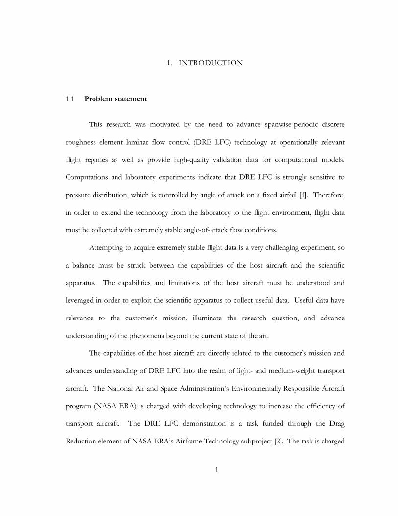
Problem statement 1.1

This research was motivated by the need to advance spanwise-periodic discrete

roughness element laminar flow control (DRE LFC) technology at operationally relevant

flight regimes as well as provide high-quality validation data for computational models.

Computations and laboratory experiments indicate that DRE LFC is strongly sensitive to

pressure distribution, which is controlled by angle of attack on a fixed airfoil [1]. Therefore,

in order to extend the technology from the laboratory to the flight environment, flight data

must be collected with extremely stable angle-of-attack flow conditions.

Attempting to acquire extremely stable flight data is a very challenging experiment, so

a balance must be struck between the capabilities of the host aircraft and the scientific

apparatus. The capabilities and limitations of the host aircraft must be understood and

leveraged in order to exploit the scientific apparatus to collect useful data. Useful data have

relevance to the customer’s mission, illuminate the research question, and advance

understanding of the phenomena beyond the current state of the art.

The capabilities of the host aircraft are directly related to the customer’s mission and

advances understanding of DRE LFC into the realm of light- and medium-weight transport

aircraft. The National Air and Space Administration’s Environmentally Responsible Aircraft

program (NASA ERA) is charged with developing technology to increase the efficiency of

transport aircraft. The DRE LFC demonstration is a task funded through the Drag

Reduction element of NASA ERA’s Airframe Technology subproject [2]. The task is charged

2

with increasing the Technology Readiness Level (TRL) from a laboratory environment

(TRL 4) at the Texas A&M University Flight Research Laboratory to an operationally relevant

flight environment (TRL 5) at the Dryden Flight Research Center at Edwards AFB, California

[3].

Understanding the physics of DRE LFC in a transport-relevant environment requires

a host aircraft with the capability to collect data in a flight envelope characterized by Mach

numbers, M = [0.67 – 0.75] and chord-based Reynolds numbers, Rec = [15M – 30M]. This is

approximately equal to altitude, h = [29,000 – 45,000] ft. The aircraft must have the physical

capability of hosting a flow test section designed for natural laminar flow and the capacity to

carry an instrumentation suite. Finally, the aircraft must be able to position the flow test

section at precise angles of attack and sideslip and hold that flight condition within narrow

tolerances to collect stabilized data.

Contributions of present work 1.2

The new contributions of this research are:

1. the design of a novel flight test technique,

2. the exploitation of the balance between data band and tolerance, and

3. the development of a designed experiment suitable to the practical limitations of

flight research.

These techniques enable the acquisition of sustained, continuous, operationally

relevant data with tight angle of attack tolerances for any flight research with similar

requirements. In the present investigation, these techniques enable both the understanding

3

and advancement of the DRE LFC technology as well as the validation of computational

models.

Specific to LFC, the new contributions, focused on the DRE LFC demonstration task

funded through the Drag Reduction element of NASA ERA’s Airframe Technology

subproject, include:

4. the designed experiment for the DRE geometry and flow conditions of interest

and

5. the flight research procedures which enable test safety, efficacy, and efficiency.

The analysis presented here considers the various factors that are critical to a

successful flight experiment. While these factors are applied to a laminar flow control flight

experiment, many of the flight test techniques can be applied to any flight experiment which

requires continuous, stabilized data collection within a narrow angle of attack data band across

a wide range of flight conditions. Technical, operational, and safety considerations are

addressed and practicable solutions outlined. In the planning stage, creative use of available

information is combined with engineering judgment and operational experience in order to

make a reasoned assessment. Issues are analyzed and presented with justification and

recommendations for a successful flight experiment. The recommendations are denoted by

R and tabulated in section 7 for reference.

4

2. BACKGROUND

The motivation for the current study is aircraft drag reduction. One mechanism to

realize drag reduction is the extension of the laminar boundary layer over the aircraft surface

before it transitions to turbulent flow. The set of techniques developed to this end span the

spectrum from natural laminar flow to laminar flow control to a hybrid of the two. This

section will begin with an outline of the benefits of laminar flow. The various physical

phenomena which lead to transition and the techniques used to affect the wing position

where surface transition occurs will be reviewed. Finally, previous experience in laminar flow

control flight research will be covered as it relates to the present effort.

Laminar flow control benefits 2.1

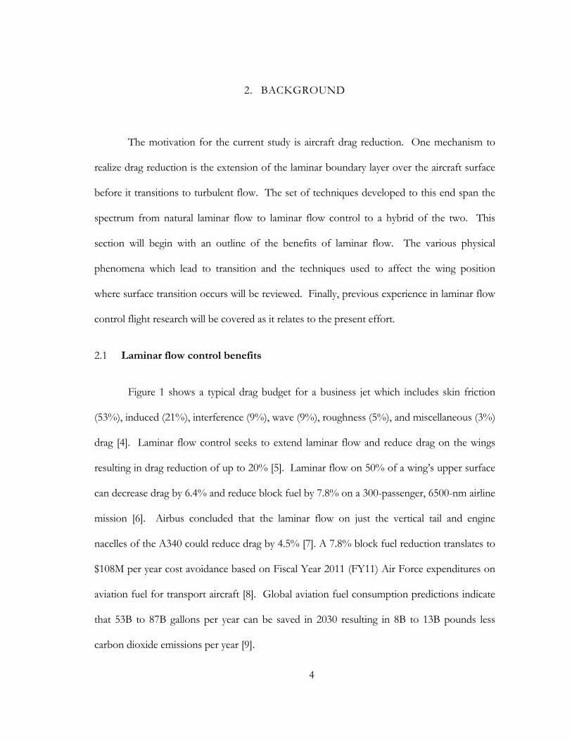
Figure 1 shows a typical drag budget for a business jet which includes skin friction

(53%), induced (21%), interference (9%), wave (9%), roughness (5%), and miscellaneous (3%)

drag [4]. Laminar flow control seeks to extend laminar flow and reduce drag on the wings

resulting in drag reduction of up to 20% [5]. Laminar flow on 50% of a wing’s upper surface

can decrease drag by 6.4% and reduce block fuel by 7.8% on a 300-passenger, 6500-nm airline

mission [6]. Airbus concluded that the laminar flow on just the vertical tail and engine

nacelles of the A340 could reduce drag by 4.5% [7]. A 7.8% block fuel reduction translates to

$108M per year cost avoidance based on Fiscal Year 2011 (FY11) Air Force expenditures on

aviation fuel for transport aircraft [8]. Global aviation fuel consumption predictions indicate

that 53B to 87B gallons per year can be saved in 2030 resulting in 8B to 13B pounds less

carbon dioxide emissions per year [9].

5

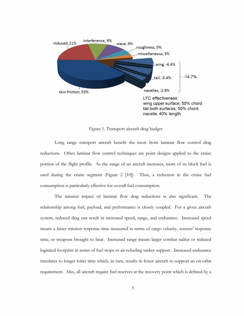
Long range transport aircraft benefit the most from laminar flow control drag

reductions. Often laminar flow control techniques are point designs applied to the cruise

portion of the flight profile. As the range of an aircraft increases, more of its block fuel is

used during the cruise segment (Figure 2 [10]). Thus, a reduction in the cruise fuel

consumption is particularly effective for overall fuel consumption.

The mission impact of laminar flow drag reductions is also significant. The

relationship among fuel, payload, and performance is closely coupled. For a given aircraft

system, reduced drag can result in increased speed, range, and endurance. Increased speed

means a faster mission response time measured in terms of cargo velocity, sensors’ response

time, or weapons brought to bear. Increased range means larger combat radius or reduced

logistical footprint in terms of fuel stops or air refueling tanker support. Increased endurance

translates to longer loiter time which, in turn, results in fewer aircraft to support an on-orbit

requirement. Also, all aircraft require fuel reserves at the recovery point which is defined by a

Figure 1. Transport aircraft drag budget

6

specific endurance requirement in a cruise configuration. A reduction in the fuel required to

meet this endurance requirement directly equates to an increase in the allowable mission fuel

or payload on every sortie.

For an aircraft system designed with the drag benefits of laminar flow control, design

tradeoffs among mission, structural, and propulsion systems have synergistic benefits. Lower

drag results in decreased thrust requirements which, in turn, enable smaller, more efficient

engines. Smaller engines require less fuel which means that fuel tanks are smaller and lighter.

Fuel weight reduction is compounded by a smaller structural mass fraction complemented by

a larger payload mass fraction. Increased payload, as the name implies, means increased value

to the customer. A study by Arcara, et al. [6] shows the value of laminar flow control to the

airline mission with 300 passengers and 6,500-nm route. The study assumes laminar flow

Figure 2. Percentage of fuel burned as a function of flight profile for subsonic transports [10]

7

control over 50% of the wing’s upper surface and both tail surfaces and result in a 5.8%

decrease in the direct operating cost from the fully turbulent airframe used as a baseline. Fuel

requirements are reduced 15% from a turbulent baseline airplane with half of the benefit due

to drag reductions on the wing [6].

Boundary layer transition mechanisms 2.2

Flight is a low disturbance environment, so laminar boundary layers transition to

turbulence through the growth of instabilities. The source of these instabilities is in four

categories: streamwise (Tollmien-Schlichting), crossflow, attachment line, and centrifugal

(Görtler). The current investigation must consider and balance the conflicting growth

characteristics of streamwise and crossflow instabilities. Airfoil construction can reduce the

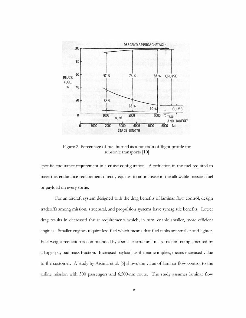
prevalence of leading-edge contamination with a Gaster bump (Figure 3 [11]) and small

leading edge radius [12]. Finally, Görtler vortices form in concave surfaces and should not be

a factor [12].

Figure 3. Gaster bump [11]

8

The viscous boundary near a wall (e.g., aircraft skin) must match the boundary

conditions of zero velocity at the wall and the local inviscid flow velocity at the edge of the

boundary layer. In two-dimensional flow, there is no inflection point in this boundary layer

profile so it is stable in the inviscid limit. However, a Reynolds stress created by the wall

viscous region destabilizes the flow and creates the Tollmien-Schlichting instability [13].

Tollmien-Schlichting waves are stabilized by a negative pressure gradient and destabilized by a

positive pressure gradient which creates an inflection point in the boundary layer velocity

profile [14].

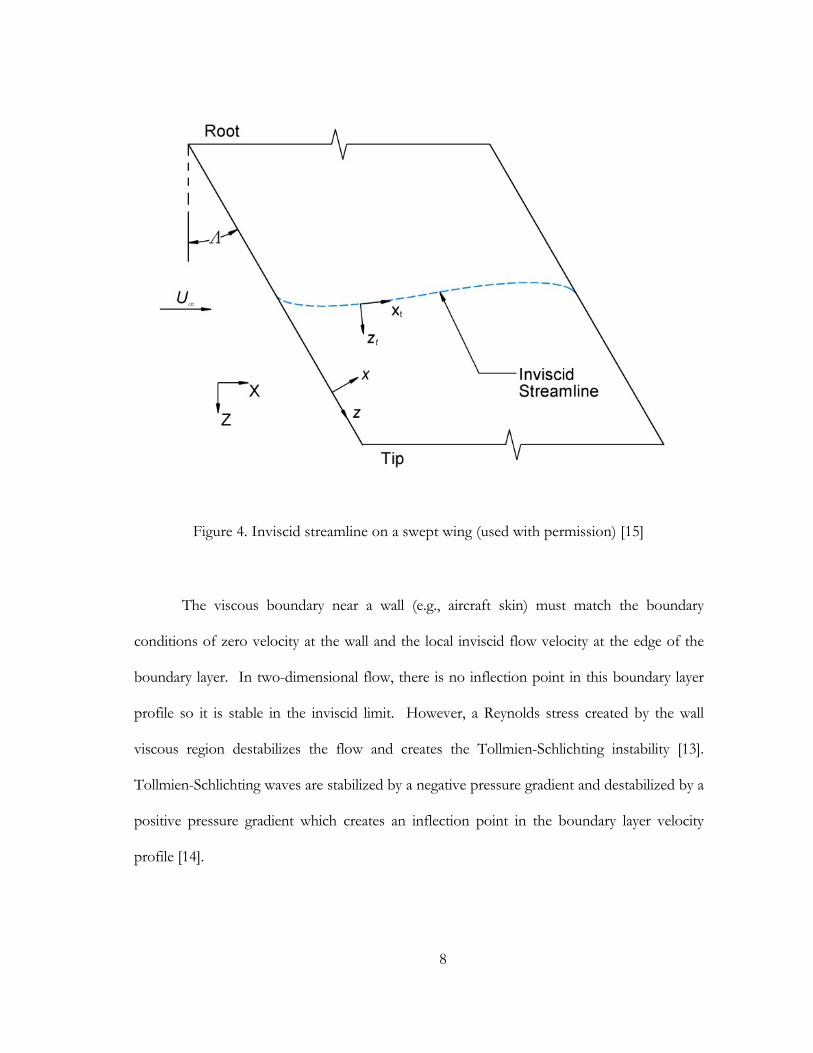
Figure 4. Inviscid streamline on a swept wing (used with permission) [15]

9

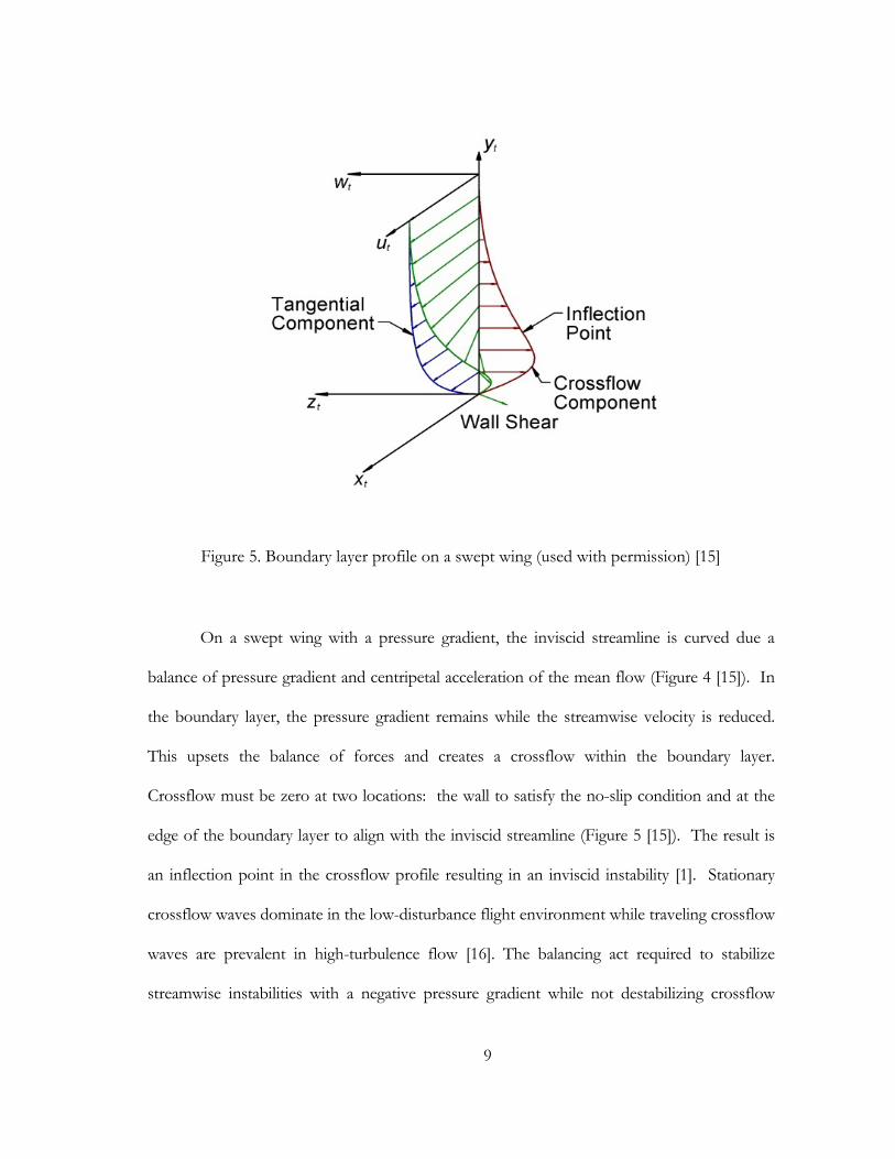
On a swept wing with a pressure gradient, the inviscid streamline is curved due a

balance of pressure gradient and centripetal acceleration of the mean flow (Figure 4 [15]). In

the boundary layer, the pressure gradient remains while the streamwise velocity is reduced.

This upsets the balance of forces and creates a crossflow within the boundary layer.

Crossflow must be zero at two locations: the wall to satisfy the no-slip condition and at the

edge of the boundary layer to align with the inviscid streamline (Figure 5 [15]). The result is

an inflection point in the crossflow profile resulting in an inviscid instability [1]. Stationary

crossflow waves dominate in the low-disturbance flight environment while traveling crossflow

waves are prevalent in high-turbulence flow [16]. The balancing act required to stabilize

streamwise instabilities with a negative pressure gradient while not destabilizing crossflow

Figure 5. Boundary layer profile on a swept wing (used with permission) [15]

10

instabilities too much is critical to the success of hybrid laminar flow control and the current

experiment.

Flight research is necessary to study boundary layer transition because of the

differences between conditions in wind tunnels and flight. First, the range of flow conditions

that can be achieved in a wind tunnel is necessarily limited by the prohibitive cost and

complexity of recreating high-speed, low-ambient-pressure flow for large-scale models.

Second, particularly for transition research, the turbulence levels in even the best wind tunnels

are greater than those in flight. Crossflow transition is sensitive to freestream turbulence

levels, so even laboratory experiments must be carried into the flight environment on such

testbeds as the Swept-wing Inflight Testbed (SWIFT) [17, 18]. Finally, the low-turbulence

flight environment is ideal for studying transition based on stationary crossflow waves [16].

Laminar flow control 2.3

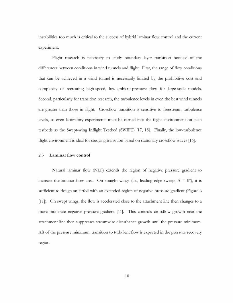
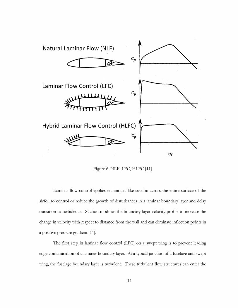
Natural laminar flow (NLF) extends the region of negative pressure gradient to

increase the laminar flow area. On straight wings (i.e., leading edge sweep, Λ = 0°), it is

sufficient to design an airfoil with an extended region of negative pressure gradient (Figure 6

[11]). On swept wings, the flow is accelerated close to the attachment line then changes to a

more moderate negative pressure gradient [11]. This controls crossflow growth near the

attachment line then suppresses streamwise disturbance growth until the pressure minimum.

Aft of the pressure minimum, transition to turbulent flow is expected in the pressure recovery

region.

11

Laminar flow control applies techniques like suction across the entire surface of the

airfoil to control or reduce the growth of disturbances in a laminar boundary layer and delay

transition to turbulence. Suction modifies the boundary layer velocity profile to increase the

change in velocity with respect to distance from the wall and can eliminate inflection points in

a positive pressure gradient [11].

The first step in laminar flow control (LFC) on a swept wing is to prevent leading

edge contamination of a laminar boundary layer. At a typical junction of a fuselage and swept

wing, the fuselage boundary layer is turbulent. These turbulent flow structures can enter the

Figure 6. NLF, LFC, HLFC [11]

12

spanwise attachment line and flow down the leading edge of the wing. Two methods of

reducing leading edge contamination are the reduction of leading edge radius and creating a

stagnation point on the leading edge. For example, if a Gaster bump is installed on the

leading edge, the turbulent flow structures will stop at the bump stagnation point (Figure 3

[11]). Laminar attachment line flow will develop from that point without disturbances. Many

laminar flow control flight experiments, including the present investigation, employ a Gaster

bump of some form to ensure laminar flow on a swept wing [19]. A 1992 Dassault Falcon 50

HLFC flight experiment noted fully turbulent flow on the test glove without a Gaster bump

even with suction. When a Gaster bump was added, after several trials with position and

wing sweep, the test glove achieved laminar flow [20].

Hybrid laminar flow control (HLFC) applies natural laminar flow principles to

suppress the growth of streamwise instabilities in conjunction with a technique such

as suction to delay transition due to crossflow instabilities. Another such technique is the

application of spanwise periodic discrete roughness elements (DRE) which work by distorting

the mean flow via a subcritical wavelength crossflow wave in such a way as to inhibit the

growth of the otherwise naturally occurring most amplified (critical) crossflow wave. DREs

are passive devices installed on the surface of the airfoil near the attachment line. Their

simplicity is attractive when compared with the additional weight and mechanical complexity

associated with the application of suction over an extended part of the surface. DRE

technology only affects crossflow instabilities, so it must be applied in a HLFC setting such as

the Texas A&M Flight Research Laboratory’s SWIFT airfoil model [12]. In the current

investigation, HLFC uses a natural laminar flow airfoil to suppress the streamwise instability

and DREs to delay crossflow transition.

13

Laminar flow control flight research 2.4

A 1942 flight investigation into laminar flow drag benefits focused on a XP-51 with a

laminar flow airfoil at 16M chord-based Reynolds number (Rec). The instrumentation

consisted of a pitot rake behind a section of wing to measure a decrease in profile drag. Data

were collected with a factory finish (10%), sanded insignia (16%), and filled and sanded

surface (24%) and compared to an unfinished airfoil [21].

In 1954, an F-94A aircraft was fitted with a wing glove featuring 69 suction slots

operated by a radial flow suction compressor. Laminar flow was achieved over the entire

glove chord at 37M Rec. The test team noted that engine noise in the Tollmien-Schlichting

frequency range may have excited boundary layer oscillations which required “surprisingly

strong” flow acceleration in the front part of the glove to stabilize the boundary layer [22].

A 1962 experiment on a Royal Air Force Lancaster bomber applied hot film

anemometers to the airfoil surface to detect laminar flow. The hot films were so physically

robust that the test team would use them to detect laminar flow then pull them off of the

wing to trail behind. Removing the hot films would eliminate the disturbances generated

from the upstream hot films and make laminar flow measurements further aft possible. The

instruments would be reaffixed on subsequent flights [23].

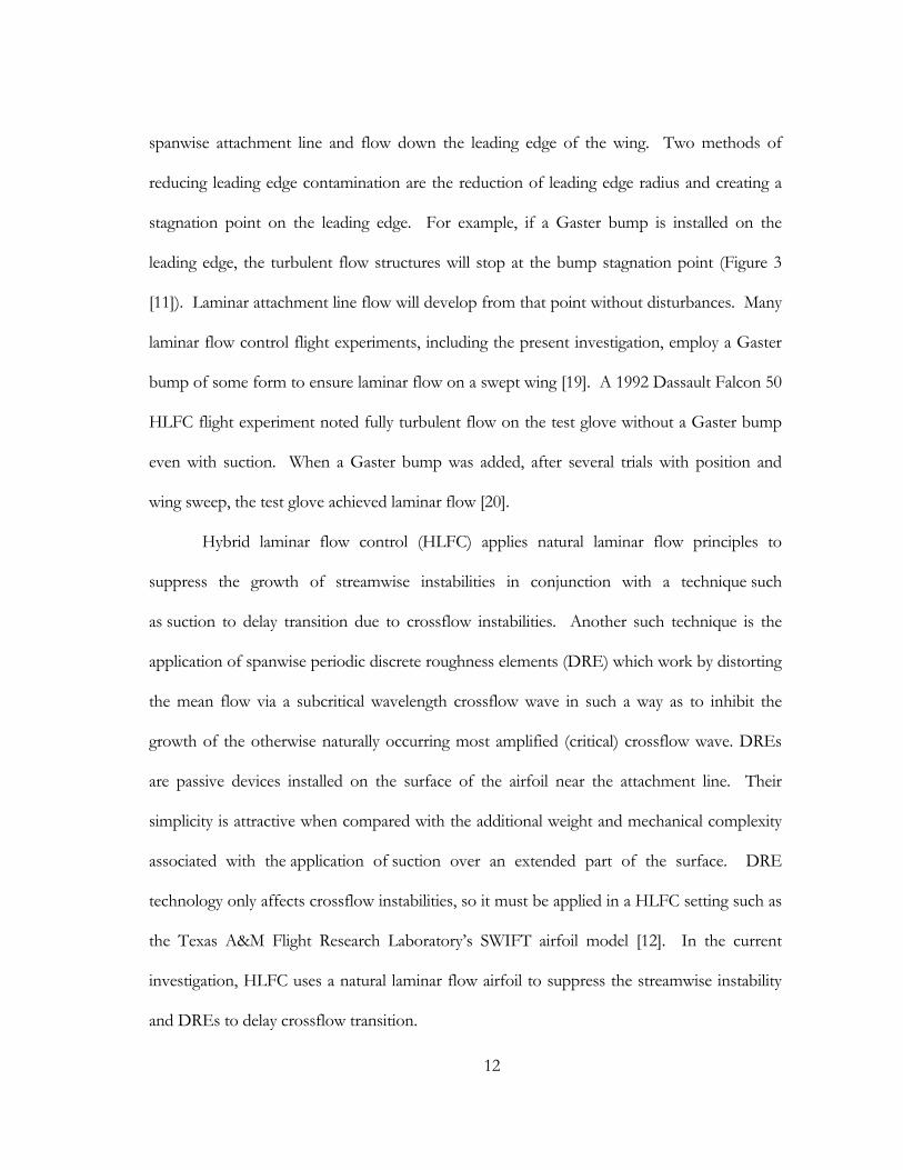
From 1960 to 1965, a WB-66 was modified with laminar flow control wings which

featured suction slots and leading edge sweep, Λ = 30°, and designated the X-21 (Figure 7

[19]). The flight envelope included Mach numbers, M = [0.3 - 0.8] and altitudes, h = [5,000 -

44,000] ft MSL. Almost 1500 hours of wind tunnel testing supported more than 200 X-21

sorties. Pressure probes were installed near the wing surface and pressure rakes measured the

14

wing wake. Microphones were mounted flush with the wing surface to collect data for

velocity fluctuation measurements and local sound levels. Throughout the program, the test

team was able to continually increase the extent of laminar flow from 0.60 to 0.96 chord, c, at

20M Rec and 0.55 to 0.81c at 30M Rec [19].

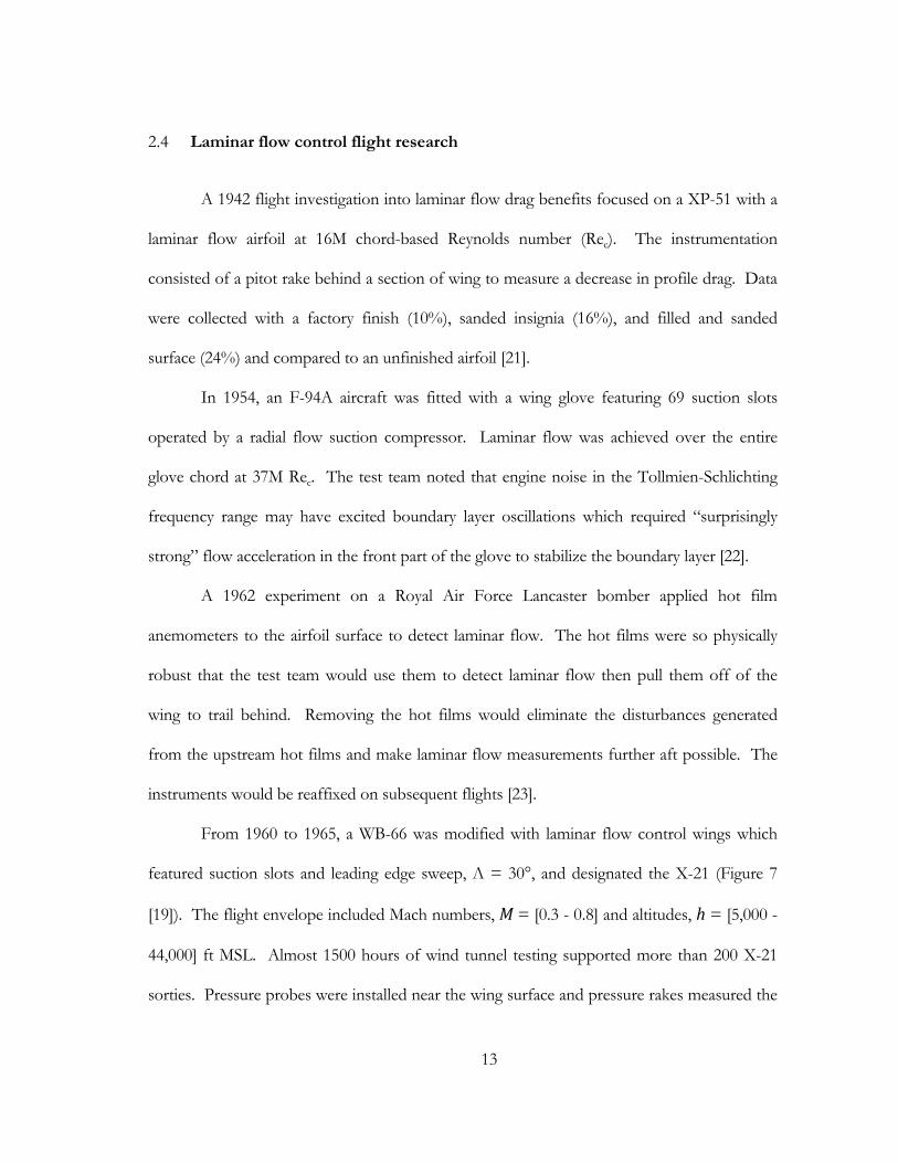
From 1983 to 1986, a National Aeronautics and Space Administration (NASA) Jetstar

aircraft was modified with two laminar flow control gloves featuring perforated- and slotted-

titanium leading edges (Figure 8 [19]). The test evaluated suction HLFC systems integration

and operational suitability through airline-style operations. A leading-edge Krueger flap

protected the right wing from insect contamination while anti-icing fluid was extruded

through the slots on the left leading edge [24]. The design test condition was selected near the

cruise flight condition of 0.75 Mach number and 38,000 ft MSL. Surface pitot probes near

the front spar were referenced to freestream pitot probes to detect boundary layer transition.

At the design condition, laminar flow was achieved for 0.74 to 0.83c and a maximum of 0.97c

for an off-design flight conditions. With the use of the Krueger flap and anti-ice fluid against

Figure 7. X-21 laminar flow control aircraft [19]

15

insect contamination, the HLFC system was determined to be suitable for airline operations

[19].

In 1987, a Boeing 757 was equipped with a perforated titanium sheet on the left wing

for HLFC research. Over 150 hours of flight research surveyed a range of Mach numbers,

Reynolds numbers, and angles of attack near cruise conditions. In addition, HLFC systems

for suction, leading edge protection, and anti-ice were evaluated. Boundary layer transition

was detected with hot films, an infrared camera, and a wake survey probe. Delay of transition

was achieved beyond 0.65c with a calculated drag reduction of 29% on the glove section [20].

A 1991 flight test program (3 flights for 12 flight hours) on a Fokker 100 measured

the drag reduction associated with a natural laminar flow wing glove at wing sweep, Λ = 20°,

Figure 8. Jetstar LFC aircraft [19]

16

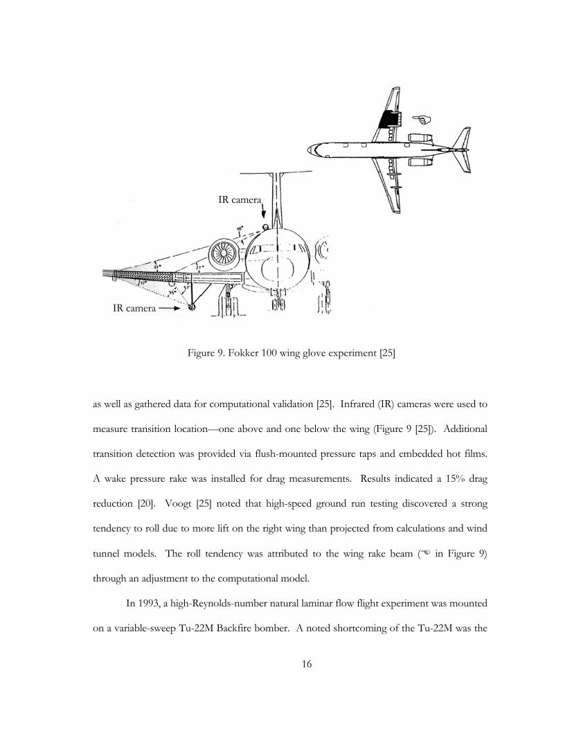
as well as gathered data for computational validation [25]. Infrared (IR) cameras were used to

measure transition location—one above and one below the wing (Figure 9 [25]). Additional

transition detection was provided via flush-mounted pressure taps and embedded hot films.

A wake pressure rake was installed for drag measurements. Results indicated a 15% drag

reduction [20]. Voogt [25] noted that high-speed ground run testing discovered a strong

tendency to roll due to more lift on the right wing than projected from calculations and wind

tunnel models. The roll tendency was attributed to the wing rake beam ( in Figure 9)

through an adjustment to the computational model.

In 1993, a high-Reynolds-number natural laminar flow flight experiment was mounted

on a variable-sweep Tu-22M Backfire bomber. A noted shortcoming of the Tu-22M was the

Figure 9. Fokker 100 wing glove experiment [25]

IR camera

IR camera

17

exclusive use of spoilers located at 0.55c for roll control. Each wing received a glove polished

to a “wind tunnel model” finish. The left glove was the baseline airfoil, and the right glove

was a laminar airfoil constructed from foam and fiberglass. The Tu-22M could achieve 25M

Rec with 20° sweep to 90M Rec with 65° sweep. However, only 20° to 28° degrees of sweep

were investigated before a collision with the chase plane while conducting infrared

thermography ended the program [26].

SWIFT laminar flow control flight research 2.5

While the previous flight research examples studied natural laminar flow and suction

HLFC, the Swept-wing Inflight Testbed (SWIFT) at the Texas A&M Flight Research

Laboratory has collected flight data on HLFC using spanwise-periodic discrete roughness

elements (DRE). It is an important step in the progression of laminar flow control research

from computational studies and wind tunnel models to flight research. SWIFT will be

discussed at length since the current flight experiment is an extension of SWIFT experiments

to transport aircraft operational relevance. Of particular note, an important difference

between SWIFT and the wing glove experiments (e.g., JetStar, B-757, Fokker 100, and Tu-

22M) is that SWIFT affects the test angle of attack on the model via aircraft sideslip. In

contrast, the wing glove design must use longitudinal control to control test angle of attack.

2.5.1 SWIFT description

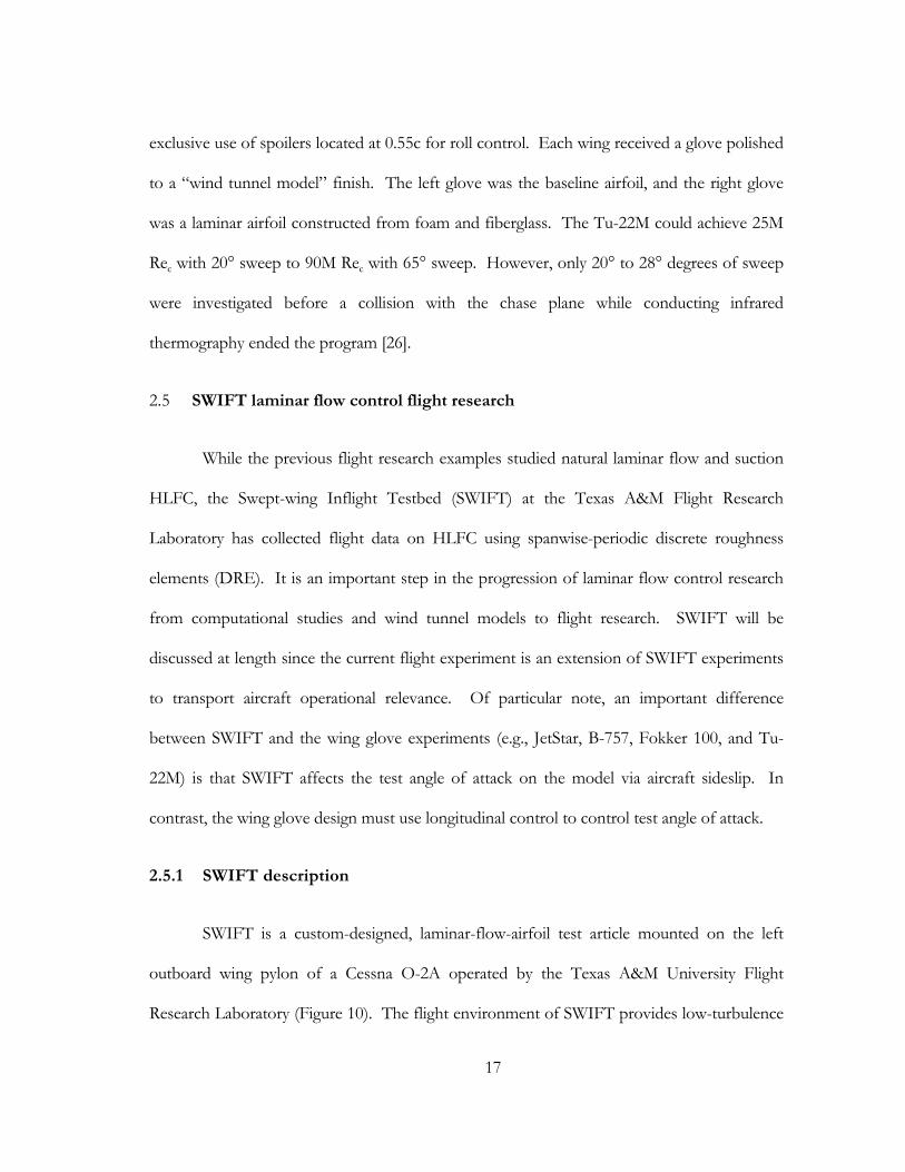
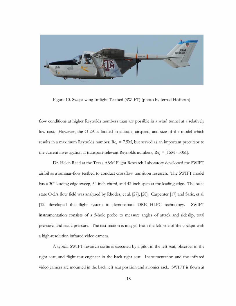
SWIFT is a custom-designed, laminar-flow-airfoil test article mounted on the left

outboard wing pylon of a Cessna O-2A operated by the Texas A&M University Flight

Research Laboratory (Figure 10). The flight environment of SWIFT provides low-turbulence

18

flow conditions at higher Reynolds numbers than are possible in a wind tunnel at a relatively

low cost. However, the O-2A is limited in altitude, airspeed, and size of the model which

results in a maximum Reynolds number, Rec = 7.5M, but served as an important precursor to

the current investigation at transport-relevant Reynolds numbers, Rec = [15M - 30M].

Dr. Helen Reed at the Texas A&M Flight Research Laboratory developed the SWIFT

airfoil as a laminar-flow testbed to conduct crossflow transition research. The SWIFT model

has a 30° leading edge sweep, 54-inch chord, and 42-inch span at the leading edge. The basic

state O-2A flow field was analyzed by Rhodes, et al. [27], [28]. Carpenter [17] and Saric, et al.

[12] developed the flight system to demonstrate DRE HLFC technology. SWIFT

instrumentation consists of a 5-hole probe to measure angles of attack and sideslip, total

pressure, and static pressure. The test section is imaged from the left side of the cockpit with

a high-resolution infrared video camera.

A typical SWIFT research sortie is executed by a pilot in the left seat, observer in the

right seat, and flight test engineer in the back right seat. Instrumentation and the infrared

video camera are mounted in the back left seat position and avionics rack. SWIFT is flown at

Figure 10. Swept-wing Inflight Testbed (SWIFT) (photo by Jerrod Hofferth)

19

10,500 ft for 20 min until the aluminum structure is a uniform temperature. A 175-KIAS dive

is initiated from 10,500 ft until the target Reynolds number, Rec = 7.5M, is attained at 5,500 to

8,000 ft MSL depending on ambient temperature. The pilot maintains the target Reynolds

number with changes to pitch attitude via a decreasing-speed, descent profile. The angle of

attack on the model is the angle of sideslip on the airplane and controlled with rudder trim.

Flight conditions are calculated from 5-hole probe data and displayed on a liquid-crystal

display (LCD) screen on the pilot’s yoke. A selected model angle of attack can be tracked

within ± 0.10°. The target Reynolds number can be tracked within ± 0.1M which equates to

an airspeed variation of approximately ± 1 KIAS. One or two dives may be executed in a

single sortie depending on the fuel available in a given test/crew configuration. Within a single

dive, several model angles of attack can be sampled, but a SWIFT configuration change

requires ground access to the model.

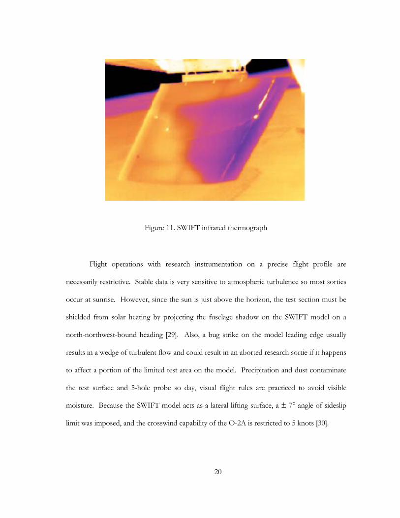
As SWIFT descends, warmer air transfers heat to the aluminum skin at different rates

depending on the overlaying boundary layer. A turbulent boundary layer transfers heat at a

much higher rate than a laminar boundary layer. The infrared camera detects the difference in

SWIFT skin temperature, and a transition front can be measured (Figure 11). Approximately

10 to 15 sec of stabilized flight conditions are required to generate the temperature differential

required to image the transition front.

20

Flight operations with research instrumentation on a precise flight profile are

necessarily restrictive. Stable data is very sensitive to atmospheric turbulence so most sorties

occur at sunrise. However, since the sun is just above the horizon, the test section must be

shielded from solar heating by projecting the fuselage shadow on the SWIFT model on a

north-northwest-bound heading [29]. Also, a bug strike on the model leading edge usually

results in a wedge of turbulent flow and could result in an aborted research sortie if it happens

to affect a portion of the limited test area on the model. Precipitation and dust contaminate

the test surface and 5-hole probe so day, visual flight rules are practiced to avoid visible

moisture. Because the SWIFT model acts as a lateral lifting surface, a ± 7° angle of sideslip

limit was imposed, and the crosswind capability of the O-2A is restricted to 5 knots [30].

Figure 11. SWIFT infrared thermograph

21

2.5.2 SWIFT pilot display evolution

The initial pilot display was a digital light-emitting diode (LED) display showing

Reynolds number and angle of sideslip that was mounted on the instrument panel glareshield.

Since this display format required the pilot to determine the parameter rate of change, a new

display was proposed. A more flexible data display would provide the exact information

required in an easily interpreted format without unnecessarily increasing the pilot workload.

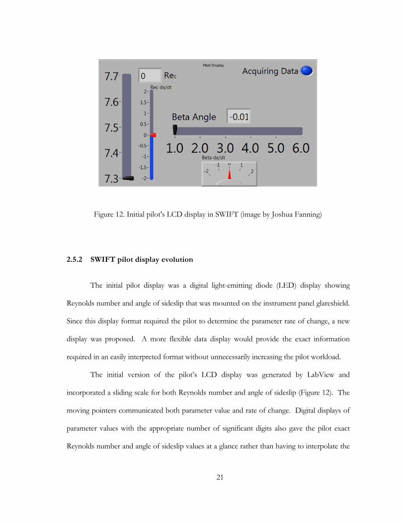
The initial version of the pilot’s LCD display was generated by LabView and

incorporated a sliding scale for both Reynolds number and angle of sideslip (Figure 12). The

moving pointers communicated both parameter value and rate of change. Digital displays of

parameter values with the appropriate number of significant digits also gave the pilot exact

Reynolds number and angle of sideslip values at a glance rather than having to interpolate the

Figure 12. Initial pilot's LCD display in SWIFT (image by Joshua Fanning)

22

values from a scale. Finally, a data health monitor was presented in the upper right corner.

The blue disk flashes when data is generated for display; conversely, the pilot can detect stale

data when the disk does not flash. This keeps the pilot from making corrections based on

false data—a potentially dangerous situation when collecting flight data near an operating

limit.

Even with the new display to show parameter rate information, the pilots were still

having difficulty tracking the desired condition without overshoot. Angle of sideslip was a

relatively steady parameter since it was set with rudder trim. Also, care was taken to minimize

bank angle inputs that could couple from the lateral axis to the directional axis. The source of

the challenge was that Reynolds number was held with pitch inputs in a descent at or near the

airspeed limit of the SWIFT model. The longitudinal short-period mode of the O-2A is

responsive enough that a time lag in the display of the pitch performance parameter was

sufficient to generate a pilot-induced oscillation (PIO). The extensive processing required to

run a graphical user interface program hosted on an operating system (e.g., LabView on

Microsoft Windows) introduces significant time lag. The time lag is measured from the time

that the 5-hold probe measures the pressure data, and LabView calculates the airspeed from

the pressure data and converts it to Reynolds number. The result is that the data trace

showed evidence of a Reynolds number PIO.

Two solutions can reduce the PIO: reduce the data lag or ask the pilot to

compensate. In order to reduce the PIO tendency, the control-feedback loop must be

shortened. The loop starts when the pressure data is measured, includes the pilot’s reaction to

the data with the resulting flight control input and the airplane’s response to the control input,

and ends with a new flight condition to be measured. The airplane flight control system

23

cannot be modified. The pilot reaction time could be replaced by an autopilot algorithm, but

that was not practical within the scope of the SWIFT program. The calculation and display of

the flow parameter could be hosted on a dedicated processor that is independent of LabView

and Microsoft Windows. Typically, time lag in a piloted system longer than 100 milliseconds

indicates PIO susceptibility [31].

In this case, the solutions were outside the scope of the project so the pilot was asked

to compensate. Upon reflection, the pilot surmised that a significant portion of the Reynolds

number perturbations were caused by variations in the temperature lapse rate. The indicated

airspeed for a given Reynolds number varies with altitude. Density is a function of pressure

and temperature through the equation of state, and viscosity is a function of temperature

through Sutherland’s Law.

Rec( , )= , , c

( ) (1)

, =R

(2)

= (Ts+C)

(T + C)

T

Ts

32 (3)

, = KIAS ( , )

(4)

As long as the temperature lapse rate was constant, the pilot could anticipate the slow

reduction in indicated airspeed required to hold a constant Reynolds number. While the

standard atmosphere model prescribes a constant temperature lapse rate, airplanes do not

operate in the standard atmosphere. A real-time display of the temperature gradient could

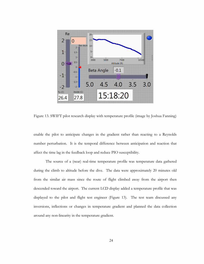
24

enable the pilot to anticipate changes in the gradient rather than reacting to a Reynolds

number perturbation. It is the temporal difference between anticipation and reaction that

affect the time lag in the feedback loop and reduce PIO susceptibility.

The source of a (near) real-time temperature profile was temperature data gathered

during the climb to altitude before the dive. The data were approximately 20 minutes old

from the similar air mass since the route of flight climbed away from the airport then

descended toward the airport. The current LCD display added a temperature profile that was

displayed to the pilot and flight test engineer (Figure 13). The test team discussed any

inversions, inflections or changes in temperature gradient and planned the data collection

around any non-linearity in the temperature gradient.

Figure 13. SWIFT pilot research display with temperature profile (image by Joshua Fanning)

25

3. TEST PLAN

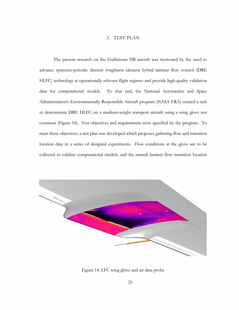
The present research on the Gulfstream IIB aircraft was motivated by the need to

advance spanwise-periodic discrete roughness element hybrid laminar flow control (DRE

HLFC) technology at operationally relevant flight regimes and provide high-quality validation

data for computational models. To that end, the National Aeronautics and Space

Administration’s Environmentally Responsible Aircraft program (NASA ERA) created a task

to demonstrate DRE HLFC on a medium-weight transport aircraft using a wing glove test

construct (Figure 14). Test objectives and requirements were specified by the program. To

meet these objectives, a test plan was developed which proposes gathering flow and transition

location data in a series of designed experiments. Flow conditions at the glove are to be

collected to validate computational models, and the natural laminar flow transition location

Figure 14. LFC wing glove and air data probe

26

measured as a baseline. Several configurations of DREs are then to be evaluated against this

baseline to evaluate their effect on transition location.

Within the test plan and subsequent sections, recommendations are made for

successful execution of the test. These recommendations called out by number (e.g., R1) and

collected at the end of this report for ease of reference.

Test objectives 3.1

The test objectives for the NASA ERA subsonic aircraft roughness glove experiment

are detailed in an operational requirements document and summarized in Belisle, et al. [32].

1. Demonstrate the aerodynamic validity of DRE HLFC technology for swept-

wing laminar flow control beyond the limits of natural laminar flow at

operationally relevant and repeatable conditions for transport aircraft.

2. Demonstrate the capability of DRE HLFC technology to repeatedly overcome

quantified small-amplitude distributed surface roughness for extended control of

cross-flow instability at roughness Reynolds numbers typical of transport aircraft.

3. Obtain repeatable and sustainable high-quality, flight-research data suitable for

evaluating the physical processes associated with the Tollmien-Schlichting and

crossflow transition mechanisms for verification and improvement of design and

analysis tools.

4. Demonstrate pressure-side laminar flow simultaneously with suction side laminar

flow.

27

Test requirements 3.2

1. Natural laminar flow (NLF) shall be demonstrated at Rec ≥ 15M with tr≥ 0.60c

on the suction side over 14 in of span. The chord-based Reynolds number, Rec, is

referenced to the chord at the mid-span of the glove.

2. DRE shall extend laminar flow at Rec ≥ 22M on the suction side by at least 50%.

3. DRE effectiveness shall be demonstrated at Re′ ≥ 1.4M/ft.

4. NLF and DRE application shall be demonstrated at leading edge sweep, Λ ≥ 30°.

5. Transport-relevant section loading shall be designed to a ℓ= 0.5 referenced to

the local glove chord within the laminar flow span.

6. Transport-relevant section loading shall be designed to Mach number, M ≥ 0.72.

7. Repeatable data shall be obtained at a repeatable and stabilized flight condition

(i.e., altitude, Mach number, etc.)

8. Passive DRE appliqué shall be used.

9. Glove design shall include the capability to vary leading edge roughness from

approximately 0.3 μm RMS to 4 μm RMS.

10. Simultaneous pressure-side and suction-side laminar flow should be demonstrated

at the flight conditions prescribed for the NLF requirement.

Experimental science envelope 3.3

The experimental science envelope is based on the mission to demonstrate natural

laminar flow and DRE effectiveness in a flight regime relevant to transport-category aircraft

(Figure 15 [33]). The data points have been described by Mach number and Reynolds number

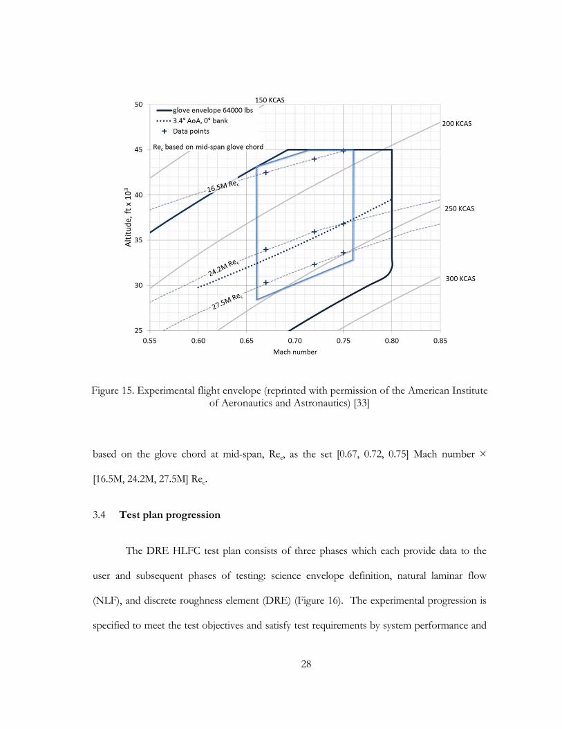
28

based on the glove chord at mid-span, Rec, as the set [0.67, 0.72, 0.75] Mach number ×

[16.5M, 24.2M, 27.5M] Rec.

Test plan progression 3.4

The DRE HLFC test plan consists of three phases which each provide data to the

user and subsequent phases of testing: science envelope definition, natural laminar flow

(NLF), and discrete roughness element (DRE) (Figure 16). The experimental progression is

specified to meet the test objectives and satisfy test requirements by system performance and

Figure 15. Experimental flight envelope (reprinted with permission of the American Institute of Aeronautics and Astronautics) [33]

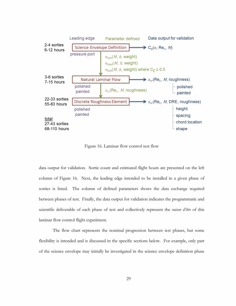
29

data output for validation. Sortie count and estimated flight hours are presented on the left

column of Figure 16. Next, the leading edge intended to be installed in a given phase of

sorties is listed. The column of defined parameters shows the data exchange required

between phases of test. Finally, the data output for validation indicates the programmatic and

scientific deliverable of each phase of test and collectively represent the raison d’être of this

laminar flow control flight experiment.

The flow chart represents the nominal progression between test phases, but some

flexibility is intended and is discussed in the specific sections below. For example, only part

of the science envelope may initially be investigated in the science envelope definition phase

Figure 16. Laminar flow control test flow

30

before continuing on to the NLF phase of data collection for that part of the science

envelope.

Science envelope definition sorties 3.5

The purpose of the science envelope definition sorties is to define the angle of attack

data band that supports crossflow transition research. The predicted cost is 2 to 4 sorties and

6 to 12 flight hours. The experimental configuration that enables this capability is the glove

leading edge equipped with pressure ports used to measure the glove pressure distribution and

a research air data boom [32]. Both the natural laminar flow and discrete roughness element

sorties depend on these data to ensure that they operate at the glove design condition and can

fulfill test requirements of crossflow transition and section loading.

A primary task of the science envelope definition sorties is to calibrate the air data

boom. Even though the five-hole probe is calibrated at the factory using a calibration rig, the

test team must determine the installation error. The least expensive method is to use the

aircraft production air data system as the truth source for airspeed and altitude (dynamic and

static pressure). Modern total temperature probes are not subject to installation errors, so a

ground calibration source will suffice. Angles of attack and sideslip are derived from

differential pressure measurements among the probe’s five holes and will be as accurate as the

installation alignment. Angle of attack alignment does not need to reference a specific angle

or flight condition, but the data should be repeatable throughout the experiment. A precise

alignment procedure should be defined for initial and interim alignment checks. A simple

visual check against alignment marks on the fuselage may be sufficient to determine

deviations in the angle of attack axis as described in the designed experiments section.

31

Angle of sideslip alignment is also important. Provisions must be made to align the

probe with the aircraft’s center plane within the angle of sideslip tolerance, βtol = 0.1°. This

may be accomplished via chalk lines on the ground marked with the aid of a plumb bob.

Both the vertical and lateral alignment of the air data probe should be checked before and

after each flight to detect changes immediately and avoid collecting flight data with an

unknown airdata probe alignment.

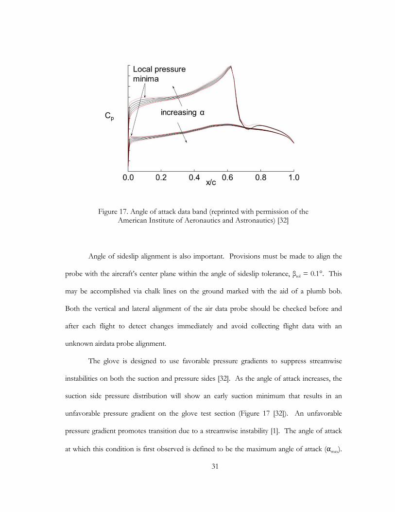
The glove is designed to use favorable pressure gradients to suppress streamwise

instabilities on both the suction and pressure sides [32]. As the angle of attack increases, the

suction side pressure distribution will show an early suction minimum that results in an

unfavorable pressure gradient on the glove test section (Figure 17 [32]). An unfavorable

pressure gradient promotes transition due to a streamwise instability [1]. The angle of attack

at which this condition is first observed is defined to be the maximum angle of attack (αmax).

Figure 17. Angle of attack data band (reprinted with permission of the American Institute of Aeronautics and Astronautics) [32]

32

As angle of attack decreases, a local pressure minimum develops near the leading edge of the

pressure side of the glove. The presence of this early pressure minimum defines the

minimum angle of attack (αmin). Both αmin and αmax are referenced to the five-hole airdata

probe measurement which must be reproduced on subsequent research flights in order to

reproduce the flow conditions on the glove.

The absolute values of αmin and αmax are not meant to relate to any angles on the

Gulfstream IIB air data system but rather a mapping from aircraft Mach number, altitude, and

weight can be determined [28]. A data band needs to be several times larger than the

parameter tolerance for good flight test efficiency. This allows the test team to sample valid

data anywhere within the data band and maintain that parameter within tolerance to meet the

stabilized data requirement.

The angle of attack data band is predicted to be the range α = [3.2°, 4.0°] based on

computational models [34]. These computations are based on free stream flow conditions

and will not be the same as local flow conditions measured at the five-hole data probe.

Rhodes, et al. [28] has established a technique to relate freestream flow conditions to specific

local flow conditions such as the air data boom or glove test surface. These computational

values are appropriate to be used to determine if the glove angle of attack data band is

compatible with the Gulfstream IIB host aircraft in the suitability planning section.

At each flight condition (i.e., Mach number, altitude), the test team records flight

parameters necessary to develop the appropriate angle of attack prediction algorithm. Fuel

weight is necessary to support a wing deflection model. Bank angle can be used with fuel

weight to calculate the effective weight of the aircraft. Infrared thermography video data is

collected to support initial evaluations of glove flow quality and transition location. Visible

33

spectrum video will capture images with optical targets on the wing, glove, and spoilers to

determine wing deflection and bending and spoiler deflection data. The five-hole airdata

probe will generate angles of attack and sideslip as well as pitot static pressures and

temperature data. Finally, the static pressure ports on the glove leading edge and test section

provide the pressure distributions necessary to determine section lift loading and validate

computational models. Drake and Solomon [35] used a similar approach to determine the

appropriate angle of attack for a swept-wing model installed under the White Knight aircraft

with good agreement between observed and calculated pressure distributions. Time

synchronization of the data streams is critical to properly align the data in the dynamic flight

research environment.

To guide the remaining testing, the test team will determine the angle of attack that

generates a section lift coefficient, ℓ= 0.5, to meet the requirement for a transport-relevant

section lift coefficient at M ≥ 0.72 and Rec ≥ 22M for DRE effectiveness. This angle of

attack (αtest) will serve as a target in the angle of attack data band that exists in the range of the

data band reduced by the angle of attack tolerance (αtol). The test team can operate at αtest and

not exceed the limits of the data band while enjoying the full extent of the tolerance.

After the pressure port leading edge is removed, the test team will not be able to

measure the pressure distribution forward of 0.15c which is where the local pressure minima

are expected to occur at αmin and αmax. However, the pressure ports on the glove test section

will continue to be monitored throughout the research test points for divergence from the

reference angles of attack. If the test team discovers that the glove test section pressure

distribution no longer matches a given set of airdata boom measurements, an additional sortie

34

configured with the pressure-port leading edge may be in order. Also, the mapping from

aircraft parameters to probe measurements can indicate a drift in prescribed glove test

conditions from sortie to sortie. Additional measurements with the pressure-port leading

edge will serve to quantify the random error of the experiment.

(R 1) Periodically fly the pressure-port leading edge to ensure valid glove flow conditions.

(R 2) Monitor test section pressure ports for changes with reference to test angle of attack.

The pressure port measurements can change due to a drift of the pressure transducers

that support the five-hole probe or change in the airdata boom alignment. Research-quality

pressure transducers are selected to reduce the risk of a drift in the output angles of attack and

airspeed which would change the glove flow conditions for a flight condition specified by the

output of the five-hole probe [36]. A change in the alignment of the five-hole probe can be

the result of improper ground handling of the supporting airdata boom. For instance, during

general servicing of the aircraft, extreme care must be taken to protect the airdata boom from

any contact. Also, due to the proximity of the airdata boom to the glove leading edge, the

airdata boom must not be contacted.

(R 3) Develop procedures to avoid contact with the airdata boom during ground operations.

Natural laminar flow sorties 3.6

The purpose of the natural laminar flow (NLF) sorties is to define the relationship

between Reynolds number and transition location on the glove test section using both painted

and polished leading edges e.g., Figure 18 [15, 34, 37]. The requirement is that NLF tr≥

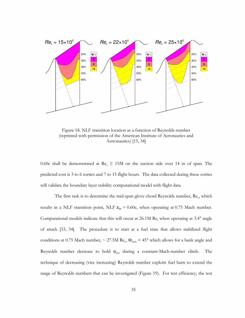
35

0.60c shall be demonstrated at Rec ≥ 15M on the suction side over 14 in of span. The

predicted cost is 3 to 6 sorties and 7 to 15 flight hours. The data collected during these sorties

will validate the boundary layer stability computational model with flight data.

The first task is to determine the mid-span glove chord Reynolds number, Rec, which

results in a NLF transition point, NLF tr= 0.60c, when operating at 0.75 Mach number.

Computational models indicate that this will occur at 26.1M Rec when operating at 3.4° angle

of attack [33, 34]. The procedure is to start at a fuel state that allows stabilized flight

conditions at 0.75 Mach number, ~ 27.5M Rec, Φlimit = 45° which allows for a bank angle and

Reynolds number decrease to hold αtest during a constant-Mach-number climb. The

technique of decreasing (vice increasing) Reynolds number exploits fuel burn to extend the

range of Reynolds numbers that can be investigated (Figure 19). For test efficiency, the test

Figure 18. NLF transition location as a function of Reynolds number (reprinted with permission of the American Institute of Aeronautics and

Astronautics) [15, 34]

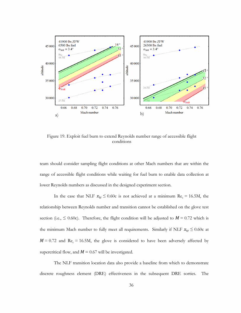
36

team should consider sampling flight conditions at other Mach numbers that are within the

range of accessible flight conditions while waiting for fuel burn to enable data collection at

lower Reynolds numbers as discussed in the designed experiment section.

In the case that NLF tr≤ 0.60c is not achieved at a minimum Rec = 16.5M, the

relationship between Reynolds number and transition cannot be established on the glove test

section (i.e., ≤ 0.60c). Therefore, the flight condition will be adjusted to M = 0.72 which is

the minimum Mach number to fully meet all requirements. Similarly if NLF tr≤ 0.60c at

M = 0.72 and Rec = 16.5M, the glove is considered to have been adversely affected by

supercritical flow, and M = 0.67 will be investigated.

The NLF transition location data also provide a baseline from which to demonstrate

discrete roughness element (DRE) effectiveness in the subsequent DRE sorties. The

Figure 19. Exploit fuel burn to extend Reynolds number range of accessible flight conditions

a) b)

37

requirement to demonstrate a 50% increase from NLF trto DRE trmeans that the flight

condition that results in NLF tr≤ 0.40c must be determined in the range Rec = [24.2M -

27.5M]. This allows for demonstration of DRE trwithin the confines of the glove test

section that ends at 0.60c (i.e., a 50% delay in transition location from 0.40c).

If NLF tr> 0.40c at Rec = 27.5M, M = 0.75, then DRE effectiveness cannot be

demonstrated to satisfy the test requirement. Two options are available to move the

transition front forward: increase the maximum Reynolds number or change the roughness

on the leading edge. An increase in maximum Reynolds number at constant Mach number

results in an increase in dynamic pressure and aerodynamic loads on the glove. Such a change

in an test limit should not be undertaken real-time but after appropriate aerodynamic loads

and flutter analysis. Increasing the leading edge roughness should also move the NLF

transition location forward and is accomplished via configuration change from a polished

leading edge (0.3 μm) to a painted leading edge (4.0 μm).

Discrete roughness element sorties 3.7

The purpose of discrete roughness element (DRE) sorties is to determine the effect of

DREs on transition location (DRE tr) compared to the previously determined NLF

transition location (NLF tr). The evaluation criterion is a 50% increase from NLF trto

DRE trin the range Rec = [24.2M - 27.5M]. For example, the flight condition that results in

NLF tr= 0.40c must result in DRE tr≥ 0.60c. Additionally, DREs must demonstrate

effectiveness when configured on a painted leading edge (4 μm RMS). Finally, the flow

38

condition and transition data will be used to validate computational models. The predicted

cost is 16 to 32 sorties and 40 to 80 flight hours.

Changing DRE configurations takes several hours on the ground, and multiple DRE

configurations are available for testing:

1. Leading edge surface condition [polished (0.3 μm RMS), painted (4 μm RMS)]

2. Height [1x, 2x, 3x, 4x, 5x] where x ~ 10 μm

3. Shape [circle, square, rounded rectangle]

4. Spacing [control (λ ~ 3 mm); 7 mm, most amplified]

As in the NLF sorties, the effect of Reynolds number on transition location will be

determined in a constant-Mach-number climb. DRE trwill be measured using infrared

thermography and will span the range [0.15c – 0.60c]. Initially, M = 0.75 will be investigated.

If the 50% increase criterion is not achieved, then the procedure will be repeated for

M = [0.72, 0.67].

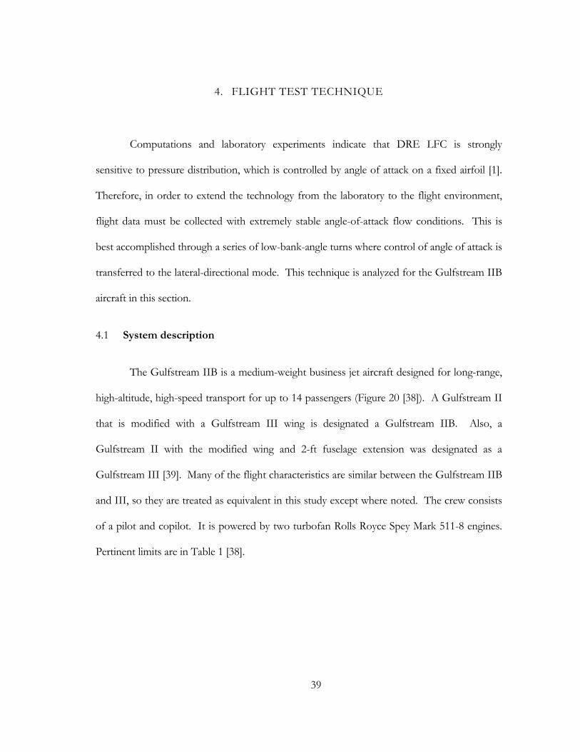
39

4. FLIGHT TEST TECHNIQUE

Computations and laboratory experiments indicate that DRE LFC is strongly

sensitive to pressure distribution, which is controlled by angle of attack on a fixed airfoil [1].

Therefore, in order to extend the technology from the laboratory to the flight environment,

flight data must be collected with extremely stable angle-of-attack flow conditions. This is

best accomplished through a series of low-bank-angle turns where control of angle of attack is

transferred to the lateral-directional mode. This technique is analyzed for the Gulfstream IIB

aircraft in this section.

System description 4.1

The Gulfstream IIB is a medium-weight business jet aircraft designed for long-range,

high-altitude, high-speed transport for up to 14 passengers (Figure 20 [38]). A Gulfstream II

that is modified with a Gulfstream III wing is designated a Gulfstream IIB. Also, a

Gulfstream II with the modified wing and 2-ft fuselage extension was designated as a

Gulfstream III [39]. Many of the flight characteristics are similar between the Gulfstream IIB

and III, so they are treated as equivalent in this study except where noted. The crew consists

of a pilot and copilot. It is powered by two turbofan Rolls Royce Spey Mark 511-8 engines.

Pertinent limits are in Table 1 [38].

40

Table 1. Gulfstream IIB limits [38]

perating weight, empty ,150 lbs [40]

aximum zero fuel weight ,000 lbs

aximum ramp weight ,200 lbs

aximum takeoff weight ,700 lbs

aximum fuel weight ,300 lbs

aximum operating speed 0 KCAS/0.85 M

oad factor limits 0g, +2.5g

aximum operating altitude ,000 ft

ingspan ft 10 in

The autopilot installed in the GIIB is the SPZ-800 with pertinent operational limits in

Table 2 [41].

Table 2. SPZ-800 autopilot limits

aximum speed 340 KCAS

85 Mach number

inimum speed 1.2 Vstall

inimum weight 38,000 lbs

ft center of gravity 43%

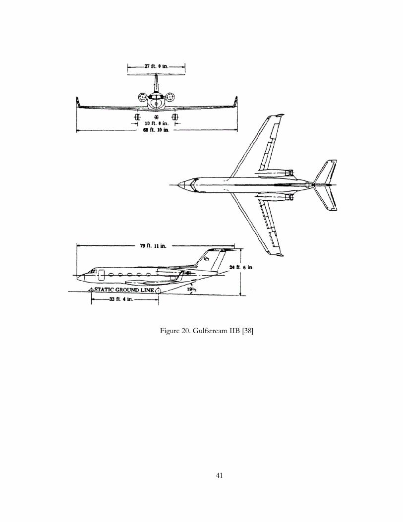
41

Figure 20. Gulfstream IIB [38]

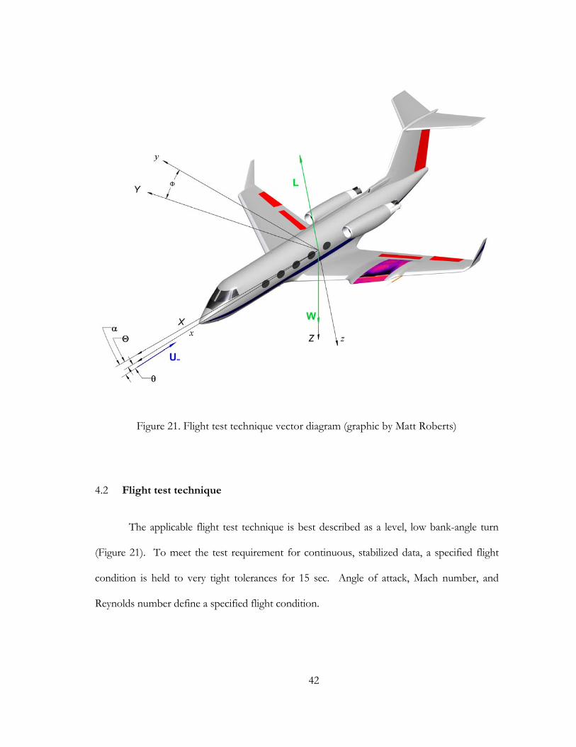
42

Flight test technique 4.2

The applicable flight test technique is best described as a level, low bank-angle turn

(Figure 21). To meet the test requirement for continuous, stabilized data, a specified flight

condition is held to very tight tolerances for 15 sec. Angle of attack, Mach number, and

Reynolds number define a specified flight condition.

Figure 21. Flight test technique vector diagram (graphic by Matt Roberts)

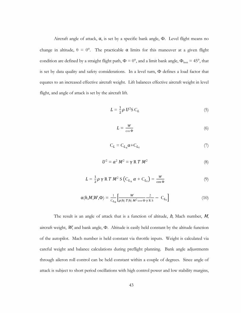
43

Aircraft angle of attack, α, is set by a specific bank angle, Φ. Level flight means no

change in altitude, θ = 0°. The practicable α limits for this maneuver at a given flight

condition are defined by a straight flight path, Φ = 0°, and a limit bank angle, Φlimit = 45°, that

is set by data quality and safety considerations. In a level turn, Φ defines a load factor that

equates to an increased effective aircraft weight. Lift balances effective aircraft weight in level

flight, and angle of attack is set by the aircraft lift.

= 2SC (5)

= cosΦ

(6)

C = C αα+C0 (7)

2 = 2 2 =γ R 2 (8)

= γ R 2 S C α + C0

= cosΦ

(9)

α( , , ,Φ) = 1

C α ( ) ( ) 2 cosΦ

2

γ R S C

0 (10)

The result is an angle of attack that is a function of altitude, h, Mach number, M,

aircraft weight, W, and bank angle, Φ. Altitude is easily held constant by the altitude function

of the autopilot. Mach number is held constant via throttle inputs. Weight is calculated via

careful weight and balance calculations during preflight planning. Bank angle adjustments

through aileron roll control can be held constant within a couple of degrees. Since angle of

attack is subject to short period oscillations with high control power and low stability margins,

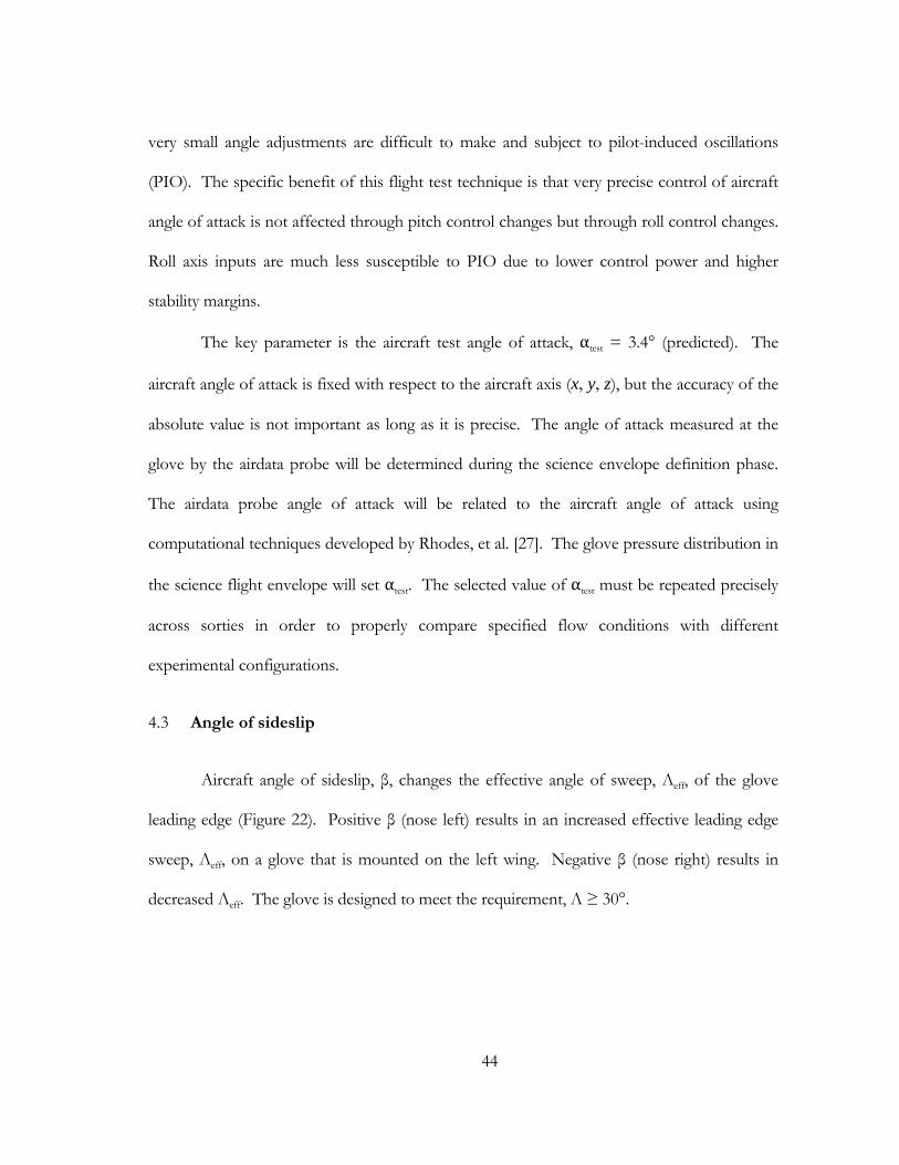
44

very small angle adjustments are difficult to make and subject to pilot-induced oscillations

(PIO). The specific benefit of this flight test technique is that very precise control of aircraft

angle of attack is not affected through pitch control changes but through roll control changes.

Roll axis inputs are much less susceptible to PIO due to lower control power and higher

stability margins.

The key parameter is the aircraft test angle of attack, αtest = 3.4° (predicted). The

aircraft angle of attack is fixed with respect to the aircraft axis (x, y, z), but the accuracy of the

absolute value is not important as long as it is precise. The angle of attack measured at the

glove by the airdata probe will be determined during the science envelope definition phase.

The airdata probe angle of attack will be related to the aircraft angle of attack using

computational techniques developed by Rhodes, et al. [27]. The glove pressure distribution in

the science flight envelope will set αtest. The selected value of αtest must be repeated precisely

across sorties in order to properly compare specified flow conditions with different

experimental configurations.

Angle of sideslip 4.3

Aircraft angle of sideslip, β, changes the effective angle of sweep, Λeff, of the glove

leading edge (Figure 22). Positive β (nose left) results in an increased effective leading edge

sweep, Λeff, on a glove that is mounted on the left wing. Negative β (nose right) results in

decreased Λeff. The glove is designed to meet the requirement, Λ ≥ 30°.

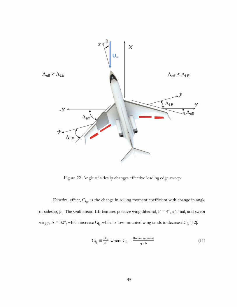
45

Dihedral effect, Cβ, is the change in rolling moment coefficient with change in angle

of sideslip, β. The Gulfstream IIB features positive wing dihedral, Γ = 4°, a T-tail, and swept

wings, Λ = 32°, which increase Cβ while its low-mounted wing tends to decrease C

β [42].

Cβ ≡

∂C

∂β where C =

Rolling moment

q S b (11)

Figure 22. Angle of sideslip changes effective leading edge sweep

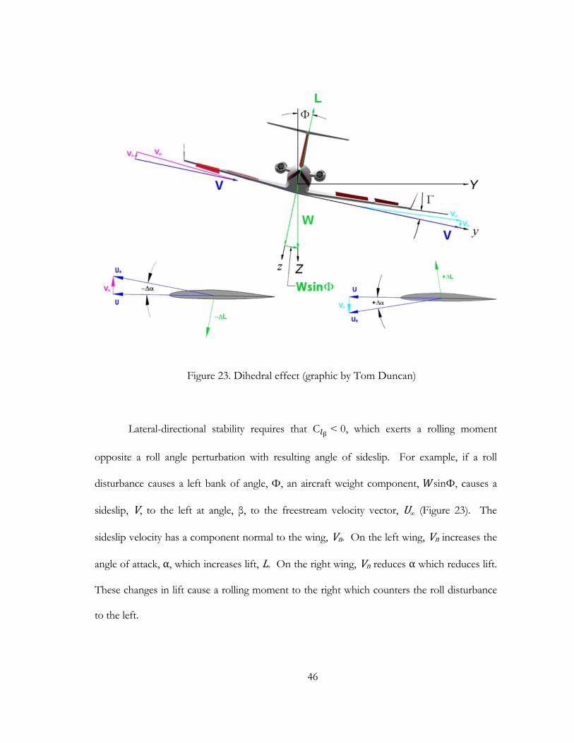
46

Lateral-directional stability requires that Cβ < 0, which exerts a rolling moment

opposite a roll angle perturbation with resulting angle of sideslip. For example, if a roll

disturbance causes a left bank of angle, Φ, an aircraft weight component, sinΦ, causes a

sideslip, V, to the left at angle, β, to the freestream velocity vector, U∞ (Figure 23). The

sideslip velocity has a component normal to the wing, Vn. On the left wing, Vn increases the

angle of attack, α, which increases lift, L. On the right wing, Vn reduces α which reduces lift.

These changes in lift cause a rolling moment to the right which counters the roll disturbance

to the left.

Figure 23. Dihedral effect (graphic by Tom Duncan)

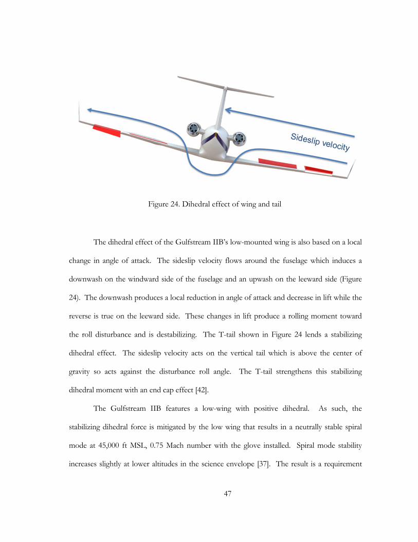
47

The dihedral effect of the Gulfstream IIB’s low-mounted wing is also based on a local

change in angle of attack. The sideslip velocity flows around the fuselage which induces a

downwash on the windward side of the fuselage and an upwash on the leeward side (Figure

24). The downwash produces a local reduction in angle of attack and decrease in lift while the

reverse is true on the leeward side. These changes in lift produce a rolling moment toward

the roll disturbance and is destabilizing. The T-tail shown in Figure 24 lends a stabilizing

dihedral effect. The sideslip velocity acts on the vertical tail which is above the center of

gravity so acts against the disturbance roll angle. The T-tail strengthens this stabilizing

dihedral moment with an end cap effect [42].

The Gulfstream IIB features a low-wing with positive dihedral. As such, the

stabilizing dihedral force is mitigated by the low wing that results in a neutrally stable spiral

mode at 45,000 ft MSL, 0.75 Mach number with the glove installed. Spiral mode stability

increases slightly at lower altitudes in the science envelope [37]. The result is a requirement

Figure 24. Dihedral effect of wing and tail

48

for small pro-turn aileron inputs to maintain a given bank angle, Φ. For example, a stable

spiral mode requires left aileron input (left aileron trailing edge up, δa < 0°) to hold a left bank

angle, Φ < 0° due to β < 0°. On the Gulfstream IIB, left aileron input is associated with left

spoiler deployment, δs, left. The NASA DFRC simulation model of a Gulfstream III with

glove shows a straight, level flight lateral trim requirement, δa, trim = +1.32°, δs, right = 2.47° at

45,000 ft MSL, 0.75 Mach number increasing to δa, trim = +1.67°, δs, right = 3.3° at 38,800 ft

MSL, 0.75 Mach number [37]. This indicates that β > 0°, which increases the effective

leading edge sweep, Λeff, of the glove on the left wing. Due to neutral to positive spiral

stability in the flight envelope, right turns should be used particularly when steep angles of

bank are required. Since the trim condition is δa > 0°, left turns using small bank angles

should also be practicable without deploying the left spoilers. The predicted lateral stability

cases at 0.75 Mach number are:

1. Right turns, 45,000 ft δa ~ δa, trim > 0°

2. Right turns, science envelope δa > δa, trim > 0°

3. Left turns, 45,000 ft δa, trim > δa > 0°

4. Left turns, science envelope δa, trim ≫ δa ? 0°

(R 4) Make turns to the right to keep left spoiler from deploying.

49

Rudder inputs also affect sideslip angle that couple into rolling moments, aileron

inputs and left spoiler deflections (Figure 25). The NASA DFRC simulation model of a

Gulfstream III with glove shows a straight, level flight rudder trim requirement,

δr, trim = +0.27° at 45,000 ft MSL, 0.75 Mach number increasing to δr,trim = +0.43° at

38,800 ft MSL, 0.75 Mach number [37]. Here, δr > 0° denotes right rudder input with rudder

trailing edge deflected to the right. Rudder can be used to affect roll control and the position

of ailerons and spoilers. For example, a left rudder input can be used to neutralize left aileron

Figure 25. Roll control due to rudder

50

input which would eliminate left spoiler. Also, left rudder input increases β which is an

increase of Λeff on the left wing.

Autopilot use 4.4

In order to reduce the variability of test, procedures should be mechanized when

possible [43]. The aircraft autopilot is critical to producing continuous, stable flight

conditions. The pitch mode of the autopilot should be used to maintain altitude which allows

the test pilots to control bank angle, Mach number, and angle of sideslip with aileron inputs,

throttle, and rudder pedals respectively. The autopilot can be engaged at bank angle,

Φ ≤ 45°. The turn knob is available to command angles of bank, Φ ≤ 32°, and touch control

steering will work for Φ ≤ 40° [41]. The test team should attempt to gather data at flight

conditions when the aircraft gross weight requires an angle of bank, Φ ≤ 32°, to stabilize at

the design angle of attack. Also, the maximum bank angle should be set at Φlimit = 45° for

data quality.

(R 5) Plan data collection at Φ ≤ 32° as much as possible.

(R 6) Set maximum bank angle, Φlimit = 45° to enable autopilot use for all data points.

Engine operation in the science envelope will be subject to flight manual

recommendations on smooth movements of the throttles. In particular, above 30,000 ft MSL

and low Mach numbers, rapid throttle movement can induce RPM stagnation or an engine

overtemperature condition. Normal throttle movement should not exceed a rate equivalent

to idle to max thrust in 4 secs [38]. Also, the flight manual recommends a minimum high

pressure turbine speed of 80% above 30,000 ft MSL [38]. Due to the characteristics of the

51

flight test technique, only small throttle movements would be required to track and maintain

specific flight conditions, so engine operating limits would not impact data collection. The

crew must be mindful of these limits, however, when transiting between flight conditions.

(R 7) Use only smooth, slow throttle movements in the science envelope.

The use of the autopilot to control pitch is reasonable based on the author’s

operational experience with transport aircraft autopilots of this milieu. Also, the Honeywell

SPZ-800 installed in the Gulfstream IIB and III has been certified by the Federal Aviation

Administration (FAA) to operate under Reduced Vertical Separation Minima (RVSM) rules

which limits altitude deviations to ± 130 ft in cruise conditions. Gulfstream test pilots report

that functional standards for an autopilot in the GIII require an altitude deviation of no more

than 20 ft in wings-level, altitude hold mode. For level turns, the Gulfstream test pilot

estimates that the autopilot altitude hold performance to be no worse than ± 40 ft [44].

Pilot display 4.5

A critical part of gathering stabilized flight data is the presentation of glove flow

conditions to the pilot. The research airdata boom near the glove provides the flow

conditions to a dedicated pilot display (Figure 26 [32]). Four performance parameters are

provided for the research pilot to control: angle of attack, Reynolds number, Mach number,

and angle of sideslip. Each are constructed of analog slider scales which feature a pointer

which deviates from a centered, desired value within a green section that indicates the

parameter tolerance. The research pilot attempts to center each of the pointers while

receiving rate of change information through the movement of the pointers. The magnitude

52

of the required correction is indicated by the displacement of the pointer from center. If the

pointers are all in the green scale, the data are within tolerances. Altitude and load factor

displays are provided for the research pilot’s situational awareness.

The slider scales are positioned on the display near the control that the research pilot

would use to effect change in that parameter. Angle of attack is on the outboard side of the

display near the research pilot’s hand on the control column. Reynolds number and Mach

number scales are positioned near the research pilot’s hand on the throttle. The angle of

sideslip scale is on the bottom near the rudder pedals.

The angle of attack scale indicates the glove angle of attack in expanded scale about

the design angle of attack. The pointer is labeled with a digital readout of the angle of attack.

The angle of attack tolerance is the first increment and is colored green to provide the pilot

with visual reinforcement for on condition. The remainder of the tick marks is situated to

encompass the full scale of angles of attack that may be encountered in the science envelope;

the pointer should not go off-scale.

The Reynolds number scale is designed to be adjusted as the test team progresses

through the test points. The center of the scale shows the current target flight condition with

tolerances bracketing a green section to indicate on condition data. The system response (i.e.,

glove transition location) is not expected to be sensitive to Mach number, so the entire

science envelope range could be displayed as in Figure 26, or an expanded scale could be

provided and adjusted real-time like the Reynolds number scale.

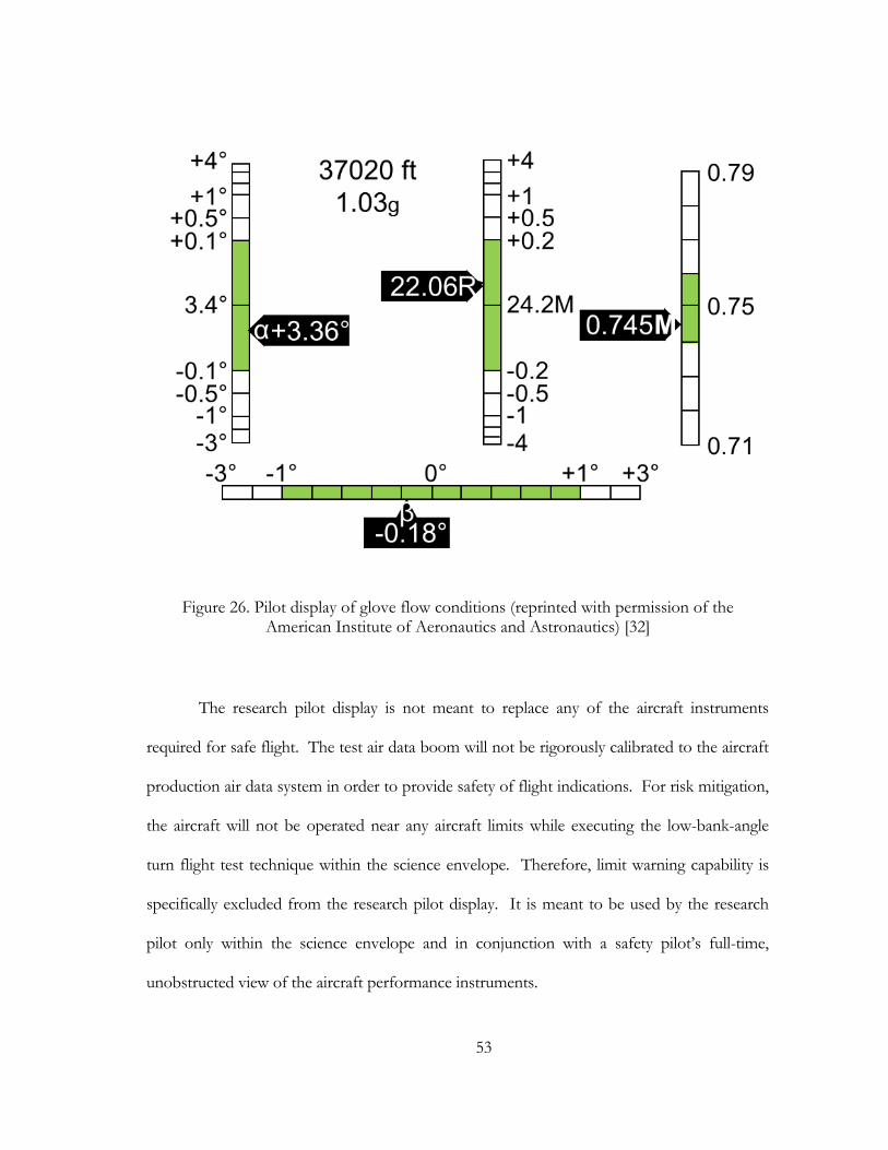
53

The research pilot display is not meant to replace any of the aircraft instruments

required for safe flight. The test air data boom will not be rigorously calibrated to the aircraft

production air data system in order to provide safety of flight indications. For risk mitigation,

the aircraft will not be operated near any aircraft limits while executing the low-bank-angle

turn flight test technique within the science envelope. Therefore, limit warning capability is

specifically excluded from the research pilot display. It is meant to be used by the research

pilot only within the science envelope and in conjunction with a safety pilot’s full-time,

unobstructed view of the aircraft performance instruments.

Figure 26. Pilot display of glove flow conditions (reprinted with permission of the American Institute of Aeronautics and Astronautics) [32]

54

Aircraft attitude and power information are intentionally not shown on the research

pilot display but are critical control parameters for the flight test technique. With that in

mind, it should be mounted so as to not obscure control instruments (e.g., attitude, engine

power) and some performance instruments (e.g., airspeed, altitude, Mach number). Other

performance instruments may be obscured for the pilot flying (e.g., heading, navigation) but

should be available to the pilot not flying to facilitate area orientation and scanning duties.

(R 8) Install the pilot display so as to not block aircraft control instruments.

The pilot display should be generated by a dedicated processor to avoid phase lag

associated with typical computer operating systems. A processing delay between sensing the

flow conditions at the glove and presenting the information to the pilot should be less than

100 ms to reduce pilot induced oscillation (PIO) susceptibility [31, 32]. If the research pilot

makes a flight control input based on performance data that is stale, and the results of that

correction are further delayed, PIO may result. Such a data lag is anathema to the research

requirement for a stabilized flight condition.

(R 9) Generate the pilot display using a dedicated processor.

Position of research airdata boom 4.6

A research air data boom is necessary to measure the flow conditions at the glove.

Therefore, the position of the air data boom is based on a compromise between a number of

factors. It should measure flow conditions that are easily related to the glove test section flow

field for computational validation. It should be outboard of the wing glove to avoid

contaminating the glove test section spanwise flow. The multi-hole probe should be located

55

in an area of low pressure and velocity gradients which is but the length of the boom is

limited by strength and flutter considerations. Finally, the boom should not present a ground

strike hazard.

Logistical requirements 4.7

Within the scope of the flight experiment, no requirement exists for a chase aircraft.

The benefits of a chase aircraft (e.g., external inspection, photography, and area clearing) do

not outweigh the cost of operation and the risk of collision. For example, the Tu-22M glove

test was cancelled after a collision with the Tu-134 chase aircraft providing infrared

thermography resulted in the deaths of all seven people onboard the chase aircraft [26]. The

very nature of a low-bank-angle turn, stabilized flight test technique within a science envelope

with sizable buffer margins from the aircraft operating limits provides substantial risk

mitigation and does not require further risk mitigation.

Walk-around oxygen bottles with smoke masks or goggles are recommended for the

research crew during research flights with the test infrared port installed. Training on the

inspection and use of oxygen walk-around bottles is required. Flight conditions above

41,000 ft MSL require one pilot to be using oxygen (FAR §91.211(3)(b)(1)(ii)). The

Gulfstream IIB flight manual figure 2-6 requires that gaseous oxygen will be used at these

altitudes at a rate of 250 psi/hour [38].

(R 10) Provide portable oxygen bottles for the research crew.

(R 11) Ensure aircraft oxygen supply is sufficient to operate above 41,000 ft MSL.

56

Communication is always a critical issue for successful flight test. Two intercom

circuits are necessary: one for the pilots and test director and one for the research crew and

test director. Normal operation allows all crew to utilize the pilot intercom but the research

crew should be able to use a separate intercom circuit to work a problem without interfering

with cockpit communications. Radio access for the research crew would be beneficial but not

critical.

(R 12) Provide a separate intercom circuit for the research crew.

A communication plan should be developed, briefed, and practiced with each new

crew member in order to qualify as part of the test team. Periodically throughout the test

program, the test team should practice the test plan together. The plan should include key

words with specific responses required (e.g., on condition, test point complete, terminate,

knock it off). It should also outline the crew position responsible for running checklists,

starting/stopping test points, calling on condition, etc. Each crew member should

demonstrate an understanding of their responsibility in an emergency and develop checklists

to support coordinated crew actions.

(R 13) Develop a communication plan for the test team.

(R 14) Develop coordinated normal and emergency checklists for the test team.

On the initial science envelope definition and natural laminar flow flights, the sortie

duration may exceed 7 hours if atmospheric conditions allow. Support for crew physical

needs will need to be provided. A lavatory must be serviceable, and an ice chest is

recommended for food and drinks.

57

(R 15) Provide functional onboard lavatory facilities for the crew.

Most of the research sorties should use the high-altitude structure within R-2508. The

test team should coordinate with Joshua Control to activate Isabella and Panamint areas from

FL290 to FL450 when appropriate. If high-altitude wave turbulence interferes with data

collection, a Warning Area off the Pacific coast may be a good alternative. If the test team

plans to operate over water, a life raft should be provided.

(R 16) Provide a life raft for the crew if operating over water for extended periods of time.

58

5. SUITABILITY PLANNING

In order to properly design the glove and flight test experiment, the performance of

the gloved aircraft must be understood. The key relationship between aircraft and glove is the

aircraft angle of attack which results in the glove test condition (αtest). This point must be

predicted as part of the glove design process but cannot be actually known until flight data are

gathered with the glove installed during the science envelope definition sorties. The following

analysis uses flight simulator data angle of attack data to determine the performance of the

Gulfstream IIB across the science envelope. The applicable Mathematica scripts are in the

Appendix.

Standard atmosphere model 5.1

A standard atmosphere model was created in the symbolic manipulator software,

Mathematica version 8.0. Constants are defined in SI units except altitude is referenced in

feet for convenience.

Constants

γ = 1.4

Specific gas constant, R = 287 m2 s-1 K-1

Gravity at sea level, g0 = 9.806 m s-2

Adiabatic lapse rate, a1 = -6.5 x 10-3 K m-1 (-1.9812 x 10-3 K ft-1)

Sea level

temperature, TS = 288.16 K

59

pressure, pS = 101,325 Pa

viscosity of air, μS = 1.7894 x 10-5 kg m-1 s-1

Temperature and pressure from sea level to the base of the tropopause, 0 ≤ h <

36,089 ft MSL:

= 1 + S (12)

= SS

-

1R (13)

Properties at the base of the tropopause, h1 = 36,089 ft:

1 = 1 1+ S = 216.66 K (14)

1 = SS

-

1R = 22,629.7 Pa (15)

Properties within the tropopause, 36,089 ft < h < 82,021 ft:

= 1 = 216.66 K (16)

= 1

- 0( - 1)R (17)

Once temperature and pressure are determined, density, ρ, and viscosity, μ, are

calculated from the equation of state and Sutherland’s Law, respectively.

= R

(18)

60

μ = μS S

32 ( S+110)

( +110) (19)

Next, the speed of sound, a, true airspeed, U, dynamic pressure, q, and Reynolds

number based on mid-span glove chord are calculated to enable performance calculations:

= γ R (20)

(21)

Rec = c

μ (22)

Angle of attack model 5.2

The three angle of attack models share a common weakness: they are predicated

upon flight simulator data. Simulator data are notoriously inaccurate with respect to flight

parameters since the emphasis for simulator flight models is handling qualities for pilot

training. Engineering models could be developed from flight test data. However, flight data

are subject to proprietary restrictions and would not typically be of research quality with

quantified accuracy and precision. Finally, only simulation models can be provided with the

glove installed. Keeping these limitations in mind, the benefits of creating such a model here

are:

1. Determine if the calculated angle of attack is predicted to allow for a

successful experiment across the entire flight envelope before glove

fabrication.

61

2. Conduct sensitivity analyses to illustrate critical parameters with respect to

fabrication, instrumentation, and test point tolerances.

3. Develop a plan of operations for the order of test points, aircraft load and fuel

requirements, and sortie duration.

NASA Dryden Flight Research center used a high-fidelity flight simulator model to

generate straight, level flight angles of attack at flight conditions across a weight range from

empty to full fuel conditions (Figure 27). The Gulfstream III-specific models included an

aerodynamics model from Flight Safety International that was an FAA level D training

simulation. The NASA DFRC Aerodynamics Branch added glove aerodynamic and mass

Figure 27. Simulator angle of attack data

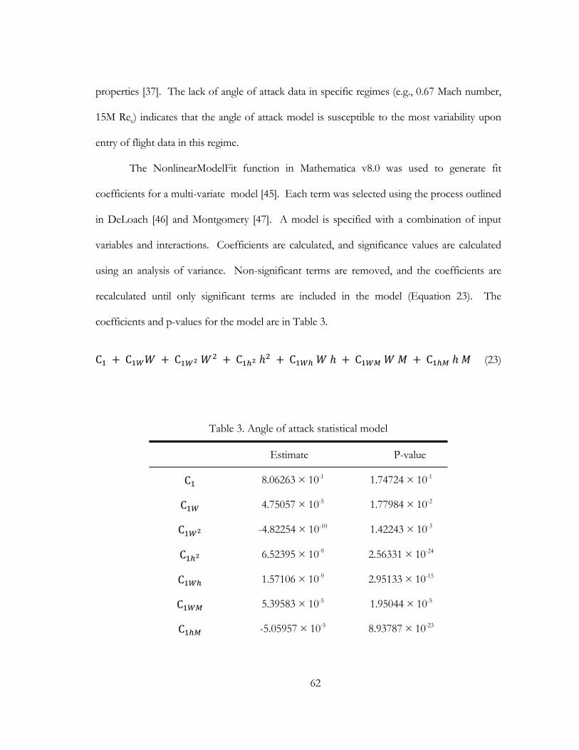
62

properties [37]. The lack of angle of attack data in specific regimes (e.g., 0.67 Mach number,

15M Rec) indicates that the angle of attack model is susceptible to the most variability upon

entry of flight data in this regime.

The NonlinearModelFit function in Mathematica v8.0 was used to generate fit

coefficients for a multi-variate model [45]. Each term was selected using the process outlined

in DeLoach [46] and Montgomery [47]. A model is specified with a combination of input

variables and interactions. Coefficients are calculated, and significance values are calculated

using an analysis of variance. Non-significant terms are removed, and the coefficients are

recalculated until only significant terms are included in the model (Equation 23). The

coefficients and p-values for the model are in Table 3.

C C C C C C C (23)

Table 3. Angle of attack statistical model

Estimate P-value

C 8.06263 × 10-1 1.74724 × 10-1

C 4.75057 × 10-5 1.77984 × 10-2

C -4.82254 × 10-10 1.42243 × 10-3

C 6.52395 × 10-9 2.56331 × 10-24

C 1.57106 × 10-9 2.95133 × 10-15

C 5.39583 × 10-5 1.95044 × 10-5

C -5.05957 × 10-5 8.93787 × 10-23

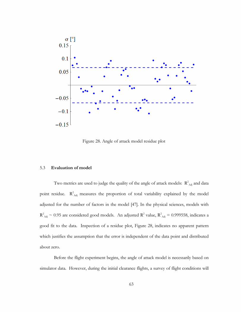
63

Evaluation of model 5.3

Two metrics are used to judge the quality of the angle of attack models: R2Adj and data

point residue. R2Adj measures the proportion of total variability explained by the model

adjusted for the number of factors in the model [47]. In the physical sciences, models with

R2Adj ~ 0.95 are considered good models. An adjusted R2 value, R2

Adj = 0.999558, indicates a

good fit to the data. Inspection of a residue plot, Figure 28, indicates no apparent pattern

which justifies the assumption that the error is independent of the data point and distributed

about zero.

Before the flight experiment begins, the angle of attack model is necessarily based on

simulator data. However, during the initial clearance flights, a survey of flight conditions will

Figure 28. Angle of attack model residue plot

64

result in angle of attack data that will replace the simulator data in the previous data set. The

resulting model can be validated with flight data, and the results used to enhance test

efficiency. The research crew can predict the required bank angle to achieve the test angle of

attack at a given flight condition (i.e., Mach number, altitude, weight). The model will also

allow the test conductor to predict the length of time that a particular flight condition can be

flown based on real-time fuel states and fuel flow rates. These techniques will allow the crew

to react to evolving weather and traffic conflicts with flexibility and efficiency.

Experimental parameters 5.4

Four important design characteristics were fixed during glove design:

Wing area, S = 86.83 m2 [40]

Lift coefficient slope, C 1.589π[48]

Glove chord, c = 4.417 m

Glove design angle of attack, αtest = 3.4° (computationally predicted aircraft angle of

attack in Roberts, et al. [34])

The characteristics of the Gulfstream IIB aircraft define several planning factors:

Bank angle limit, Φlimit = 45° (maximum bank angle based on safety, data quality

considerations)

Zero fuel weight, ZFW = 41,900 lbs (weight of the aircraft with crew and

instrumentation)

Maximum takeoff gross weight, MTOGW = 69,700 lbs [38]

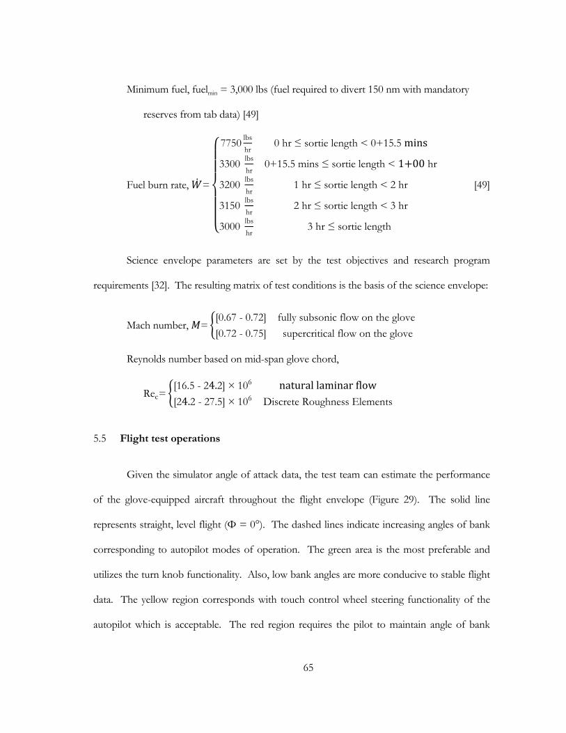
65

Minimum fuel, fuelmin = 3,000 lbs (fuel required to divert 150 nm with mandatory

reserves from tab data) [49]

Fuel burn rate, =

7750lbs

hr0 hr ≤ sortie length < 0+15.5 mins

3300 lbs

hr0+15.5 mins ≤ sortie length < 1 00 hr

3200 lbs

hr1 hr ≤ sortie length < 2 hr

3150 lbs

hr2 hr ≤ sortie length < 3 hr

3000 lbs

hr3 hr ≤ sortie length

[49]

Science envelope parameters are set by the test objectives and research program

requirements [32]. The resulting matrix of test conditions is the basis of the science envelope:

Mach number, =[0.67 - 0.72] fully subsonic flow on the glove

[0.72 - 0.75] supercritical flow on the glove

Reynolds number based on mid-span glove chord,

Rec=[16.5 - 24.2]×106 naturallaminarflow[24.2 - 27.5]×106 Discrete Roughness Elements

Flight test operations 5.5

Given the simulator angle of attack data, the test team can estimate the performance

of the glove-equipped aircraft throughout the flight envelope (Figure 29). The solid line

represents straight, level flight (Φ = 0°). The dashed lines indicate increasing angles of bank

corresponding to autopilot modes of operation. The green area is the most preferable and

utilizes the turn knob functionality. Also, low bank angles are more conducive to stable flight

data. The yellow region corresponds with touch control wheel steering functionality of the

autopilot which is acceptable. The red region requires the pilot to maintain angle of bank

66

while the pitch mode of the autopilot maintains level flight. This promises to be the least

stable and the most difficult region in which to acquire data. The maximum bank angle is

annotated by a red line that is labeled as Φlimit. Since the effective weight of the aircraft varies

with the load factor, n = (cos Φ)-1, the change in effective weight from 0° to 14° is small

compared to the change in effective weight from 32° to 45°.

In particular for a given glove design angle of attack (αtest), the ability of the

Gulfstream IIB aircraft to access the entire flight envelope is examined in light of the inherent

limitations of fuel load and maximum bank angle, Φlimit. Figure 29d shows the region of the

flight envelope that is accessible to a Gulfstream IIB flying level at αtest after departing at the

maximum takeoff gross weight (MTOGW) with a zero fuel weight (ZFW) of 41,900. Figure

29a shows the region of the flight envelope that is accessible to a Gulfstream IIB flying level

at αtest and minimum fuel load and ZFW of 37,000 lbs which would require minimum

instrumentation and very little cabin accoutrements [50, 51].

Figure 29 also gives indicates that the flight test technique is not sensitive to minor

changes in Mach number or altitude. The lines of constant angle of bank align closely with

the Mach number axis which indicates that a change in airspeed during a test point will not

require much change in the test angle of bank to achieve αtest. Also, the angle of bank bands

span several thousand feet during a level flight test technique. The expected autopilot

performance (± 40 ft) is two orders of magnitude less than the change required to

substantially affect the test angle of bank [44].

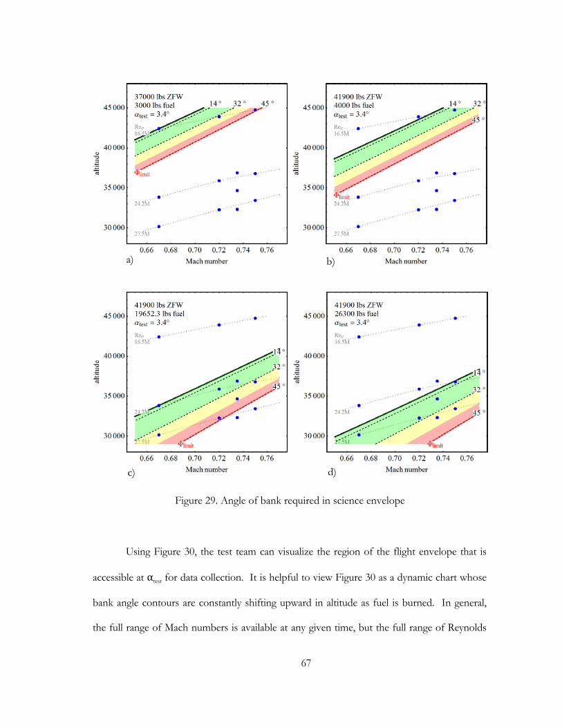
67

Using Figure 30, the test team can visualize the region of the flight envelope that is

accessible at αtest for data collection. It is helpful to view Figure 30 as a dynamic chart whose

bank angle contours are constantly shifting upward in altitude as fuel is burned. In general,

the full range of Mach numbers is available at any given time, but the full range of Reynolds

Figure 29. Angle of bank required in science envelope

d)

a) b)

c)

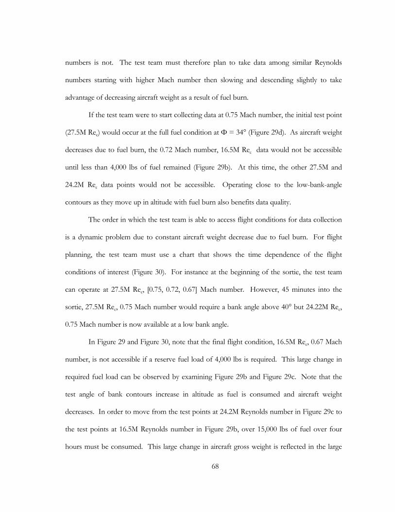
68

numbers is not. The test team must therefore plan to take data among similar Reynolds

numbers starting with higher Mach number then slowing and descending slightly to take

advantage of decreasing aircraft weight as a result of fuel burn.

If the test team were to start collecting data at 0.75 Mach number, the initial test point

(27.5M Rec) would occur at the full fuel condition at Φ = 34° (Figure 29d). As aircraft weight

decreases due to fuel burn, the 0.72 Mach number, 16.5M Rec data would not be accessible

until less than 4,000 lbs of fuel remained (Figure 29b). At this time, the other 27.5M and

24.2M Rec data points would not be accessible. Operating close to the low-bank-angle

contours as they move up in altitude with fuel burn also benefits data quality.

The order in which the test team is able to access flight conditions for data collection

is a dynamic problem due to constant aircraft weight decrease due to fuel burn. For flight

planning, the test team must use a chart that shows the time dependence of the flight

conditions of interest (Figure 30). For instance at the beginning of the sortie, the test team

can operate at 27.5M Rec, [0.75, 0.72, 0.67] Mach number. However, 45 minutes into the

sortie, 27.5M Rec, 0.75 Mach number would require a bank angle above 40° but 24.22M Rec,

0.75 Mach number is now available at a low bank angle.

In Figure 29 and Figure 30, note that the final flight condition, 16.5M Rec, 0.67 Mach

number, is not accessible if a reserve fuel load of 4,000 lbs is required. This large change in

required fuel load can be observed by examining Figure 29b and Figure 29c. Note that the

test angle of bank contours increase in altitude as fuel is consumed and aircraft weight

decreases. In order to move from the test points at 24.2M Reynolds number in Figure 29c to

the test points at 16.5M Reynolds number in Figure 29b, over 15,000 lbs of fuel over four

hours must be consumed. This large change in aircraft gross weight is reflected in the large

69

jump between 24.2M Reynolds number and 16.5M Reynolds number flight condition

availability windows in the test point timeline (Figure 30).

There is a balance between operations and science in flight research which can be

understood with proper planning and exploited for test efficiency. For instance, the test team

could agree to operate with a higher reserve fuel load to preserve airspace flexibility for the

vast majority of the sorties. In the specific instance when the science requires a flight

condition that requires operation below the higher reserve fuel load, the test team can plan to

accept a lower reserve fuel load along with additional restrictions to mitigate the increased

risk. The test team would determine a maximum operating radius from the recovery landing

field, more restrictive weather conditions, and more conservative minimum equipment list.

Figure 30. Test conditions accessible during flight

70

These mitigating procedures would reduce the risk of routing changes, weather holds, and

mechanical delays, respectively, on the way to a safe landing.

The test team can even adjust the required reserve fuel within a sortie based on

mission elements. In a survey mission during the science envelope definition and natural

laminar flow phases, the team could start the sortie with a higher required fuel reserve and

more flexible mission rules as discussed above. As the sortie progresses, the test team

examines the mission rules to determine if the fuel state (joker fuel, in mission parlance)

allows the mission to continue under a given set of conditions. Of course, the test team also

sets a minimum fuel with which they must terminate testing and return to base (bingo fuel).

(R 17) Use multi-layered fuel reserves balance risk mitigation and the research mission.

Other considerations such as fuel loading (for wing deflection/twist effects) may

require multiple replicates of a flight condition. The first sample would occur at a low bank

angle (low in a flight condition bar in Figure 30). Data would be collected at other flight

conditions before returning to the given flight condition to gather data at a higher bank angle

(top of a flight condition bar). The skill of the test team at gathering continuous, stable data

will increase with experience. However, proper prior planning will enhance the efficiency and

efficacy of the test sorties.

The effect of Mach number on stability is expected to have a weak effect, so a test

technique that keeps a constant Mach number and allows Reynolds number to vary would be

a more interesting experiment with operational relevance. The flight test technique would

closely resemble a simple constant-Mach-number climb albeit at a very slow climb rate. The

operational equivalent is a cruise climb, which is used in uncongested airspace (e.g., oceanic

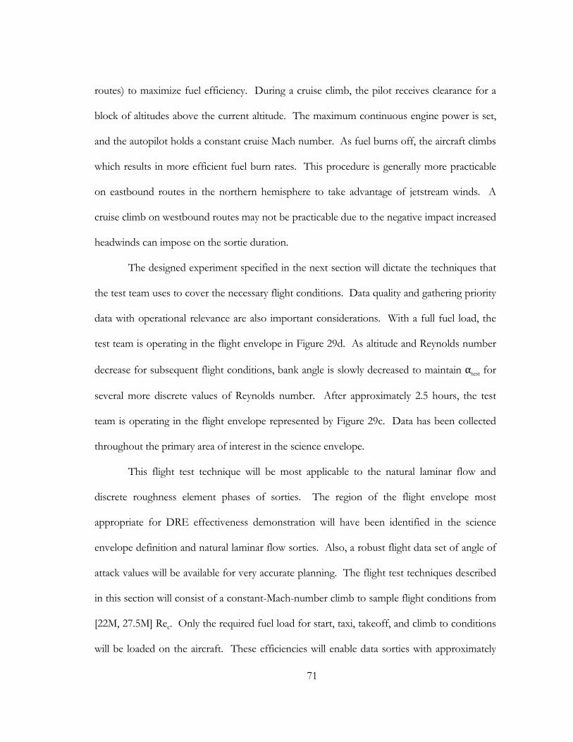
71

routes) to maximize fuel efficiency. During a cruise climb, the pilot receives clearance for a

block of altitudes above the current altitude. The maximum continuous engine power is set,

and the autopilot holds a constant cruise Mach number. As fuel burns off, the aircraft climbs

which results in more efficient fuel burn rates. This procedure is generally more practicable

on eastbound routes in the northern hemisphere to take advantage of jetstream winds. A

cruise climb on westbound routes may not be practicable due to the negative impact increased

headwinds can impose on the sortie duration.

The designed experiment specified in the next section will dictate the techniques that

the test team uses to cover the necessary flight conditions. Data quality and gathering priority

data with operational relevance are also important considerations. With a full fuel load, the

test team is operating in the flight envelope in Figure 29d. As altitude and Reynolds number

decrease for subsequent flight conditions, bank angle is slowly decreased to maintain αtest for

several more discrete values of Reynolds number. After approximately 2.5 hours, the test

team is operating in the flight envelope represented by Figure 29c. Data has been collected

throughout the primary area of interest in the science envelope.

This flight test technique will be most applicable to the natural laminar flow and

discrete roughness element phases of sorties. The region of the flight envelope most

appropriate for DRE effectiveness demonstration will have been identified in the science

envelope definition and natural laminar flow sorties. Also, a robust flight data set of angle of

attack values will be available for very accurate planning. The flight test techniques described

in this section will consist of a constant-Mach-number climb to sample flight conditions from

[22M, 27.5M] Rec. Only the required fuel load for start, taxi, takeoff, and climb to conditions

will be loaded on the aircraft. These efficiencies will enable data sorties with approximately

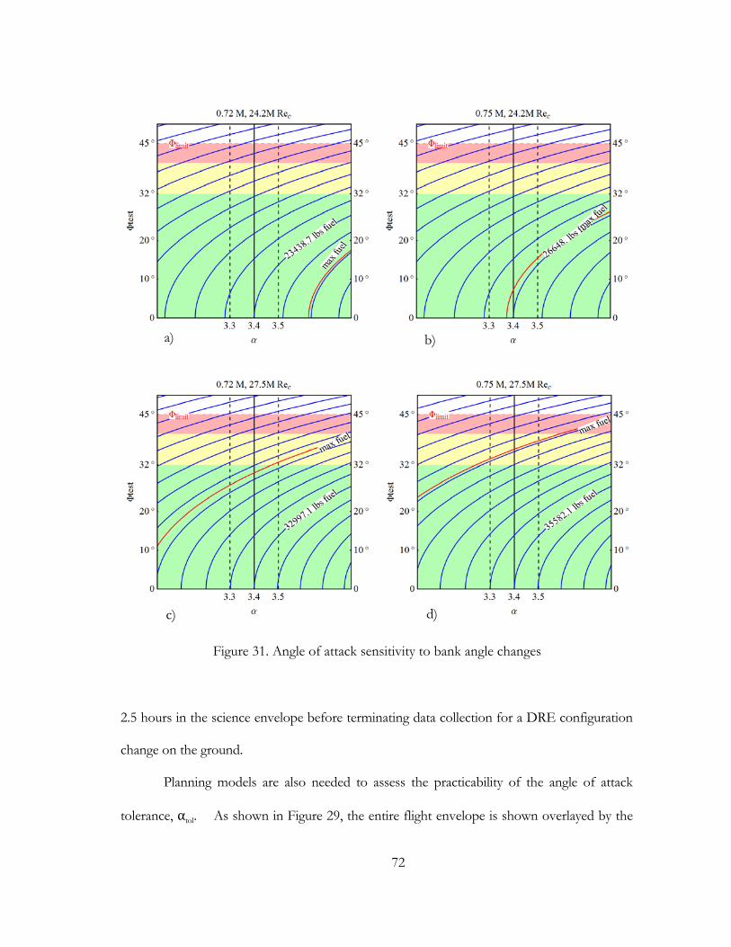
72

2.5 hours in the science envelope before terminating data collection for a DRE configuration

change on the ground.

Planning models are also needed to assess the practicability of the angle of attack

tolerance, αtol. As shown in Figure 29, the entire flight envelope is shown overlayed by the

Figure 31. Angle of attack sensitivity to bank angle changes

d)

a) b)

c)

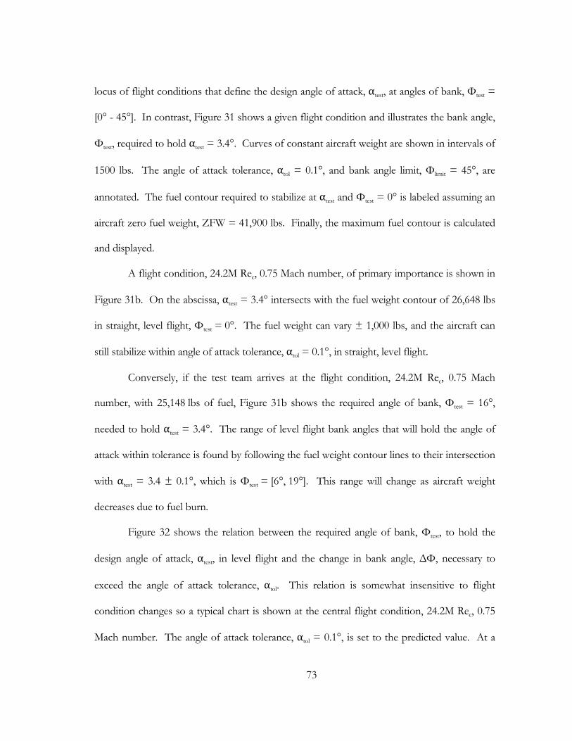
73

locus of flight conditions that define the design angle of attack, αtest, at angles of bank, Φtest =

[0° - 45°]. In contrast, Figure 31 shows a given flight condition and illustrates the bank angle,

Φtest, required to hold αtest = 3.4°. Curves of constant aircraft weight are shown in intervals of

1500 lbs. The angle of attack tolerance, αtol = 0.1°, and bank angle limit, Φlimit = 45°, are

annotated. The fuel contour required to stabilize at αtest and Φtest = 0° is labeled assuming an

aircraft zero fuel weight, ZFW = 41,900 lbs. Finally, the maximum fuel contour is calculated

and displayed.

A flight condition, 24.2M Rec, 0.75 Mach number, of primary importance is shown in

Figure 31b. On the abscissa, αtest = 3.4° intersects with the fuel weight contour of 26,648 lbs

in straight, level flight, Φtest = 0°. The fuel weight can vary ± 1,000 lbs, and the aircraft can

still stabilize within angle of attack tolerance, αtol = 0.1°, in straight, level flight.

Conversely, if the test team arrives at the flight condition, 24.2M Rec, 0.75 Mach

number, with 25,148 lbs of fuel, Figure 31b shows the required angle of bank, Φtest = 16°,

needed to hold αtest = 3.4°. The range of level flight bank angles that will hold the angle of

attack within tolerance is found by following the fuel weight contour lines to their intersection

with αtest = 3.4 ± 0.1°, which is Φtest = [6°, 19°]. This range will change as aircraft weight

decreases due to fuel burn.

Figure 32 shows the relation between the required angle of bank, Φtest, to hold the

design angle of attack, αtest, in level flight and the change in bank angle, ΔΦ, necessary to

exceed the angle of attack tolerance, αtol. This relation is somewhat insensitive to flight

condition changes so a typical chart is shown at the central flight condition, 24.2M Rec, 0.75

Mach number. The angle of attack tolerance, αtol = 0.1°, is set to the predicted value. At a

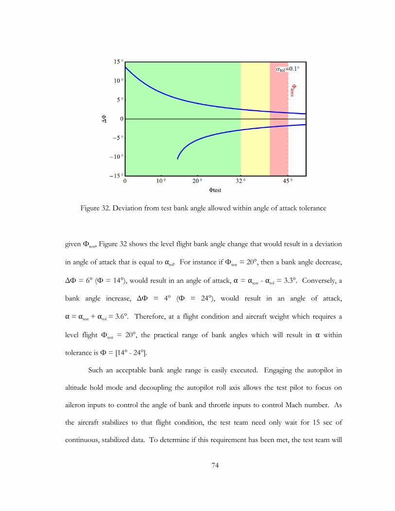
74

given Φtest, Figure 32 shows the level flight bank angle change that would result in a deviation

in angle of attack that is equal to αtol. For instance if Φtest = 20°, then a bank angle decrease,

ΔΦ = 6° (Φ = 14°), would result in an angle of attack, α = αtest - αtol = 3.3°. Conversely, a

bank angle increase, ΔΦ = 4° (Φ = 24°), would result in an angle of attack,

α = αtest + αtol = 3.6°. Therefore, at a flight condition and aircraft weight which requires a

level flight Φtest = 20°, the practical range of bank angles which will result in α within

tolerance is Φ = [14° - 24°].

Such an acceptable bank angle range is easily executed. Engaging the autopilot in

altitude hold mode and decoupling the autopilot roll axis allows the test pilot to focus on

aileron inputs to control the angle of bank and throttle inputs to control Mach number. As

the aircraft stabilizes to that flight condition, the test team need only wait for 15 sec of

continuous, stabilized data. To determine if this requirement has been met, the test team will

Figure 32. Deviation from test bank angle allowed within angle of attack tolerance

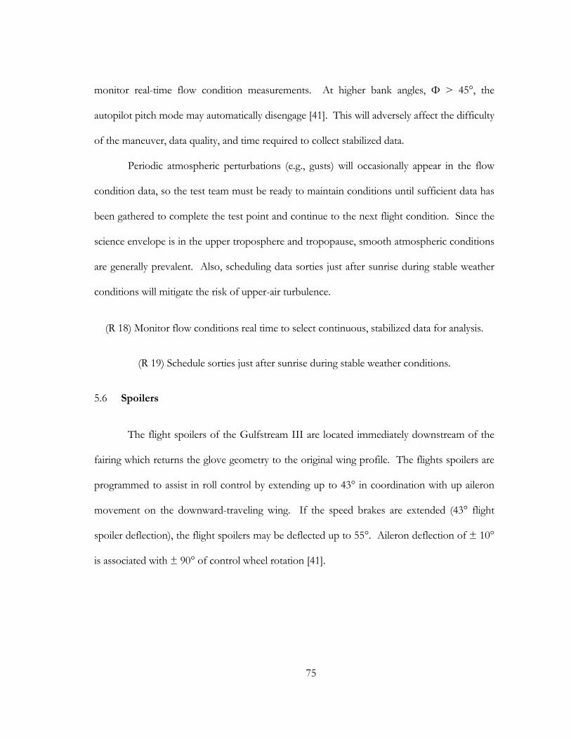
75

monitor real-time flow condition measurements. At higher bank angles, Φ > 45°, the

autopilot pitch mode may automatically disengage [41]. This will adversely affect the difficulty

of the maneuver, data quality, and time required to collect stabilized data.

Periodic atmospheric perturbations (e.g., gusts) will occasionally appear in the flow

condition data, so the test team must be ready to maintain conditions until sufficient data has

been gathered to complete the test point and continue to the next flight condition. Since the

science envelope is in the upper troposphere and tropopause, smooth atmospheric conditions

are generally prevalent. Also, scheduling data sorties just after sunrise during stable weather

conditions will mitigate the risk of upper-air turbulence.

(R 18) Monitor flow conditions real time to select continuous, stabilized data for analysis.

(R 19) Schedule sorties just after sunrise during stable weather conditions.

Spoilers 5.6

The flight spoilers of the Gulfstream III are located immediately downstream of the

fairing which returns the glove geometry to the original wing profile. The flights spoilers are

programmed to assist in roll control by extending up to 43° in coordination with up aileron

movement on the downward-traveling wing. If the speed brakes are extended (43° flight

spoiler deflection), the flight spoilers may be deflected up to 55°. Aileron deflection of ± 10°

is associated with ± 90° of control wheel rotation [41].

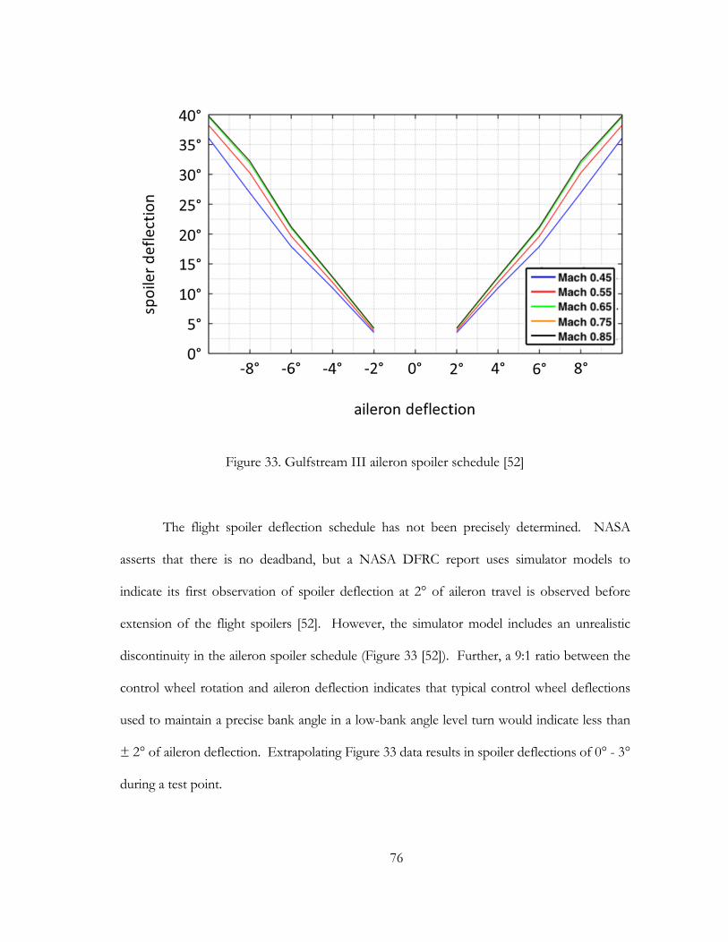
76

The flight spoiler deflection schedule has not been precisely determined. NASA

asserts that there is no deadband, but a NASA DFRC report uses simulator models to

indicate its first observation of spoiler deflection at 2° of aileron travel is observed before

extension of the flight spoilers [52]. However, the simulator model includes an unrealistic

discontinuity in the aileron spoiler schedule (Figure 33 [52]). Further, a 9:1 ratio between the

control wheel rotation and aileron deflection indicates that typical control wheel deflections

used to maintain a precise bank angle in a low-bank angle level turn would indicate less than

± 2° of aileron deflection. Extrapolating Figure 33 data results in spoiler deflections of 0° - 3°

during a test point.

Figure 33. Gulfstream III aileron spoiler schedule [52]

77

(R 20) Measure the spoiler deflection as a function of aileron input on the test aircraft.

In the interest of reducing spoiler deflection during the test points, specified rigging

tolerances can be exploited to increase the spoiler deflection deadband. The maintenance

rigging manual often provides rigging tolerances for flight control adjustment that preserve

design handling qualities. The rigging can be adjusted to the limits of the maintenance manual

tolerance that allow for a larger deadband for spoiler deflection from aileron input.

(R 21) Adjust aileron input/spoiler deflection deadband to maximum allowable.

After mitigation efforts, spoiler deflection must be measured during test execution to

account for its effects during data reduction and model validation. This deflection can be

tracked via optical targets on the flight spoiler panels and a high-resolution video camera like

that used for the wing deflection measurements. With a time stamp, the spoiler deflection can

be correlated to other instrumented properties and included in the data set.

(R 22) Use optical targets to determine spoiler deflection during test point execution.

Until a ground test on a Gulfstream III can be performed to observe the relationship

between the aileron and spoilers, the test team must plan for some spoiler deflection and

mitigate its effects. First, the effect of spoiler deflection on glove airflow must be modeled to

determine its effect on the pressure distribution. However, most test conditions experience

supercritical flow on the aft end of the glove just before the spoiler location. This shock is

limited to a small area of supercritical flow at the aft end of the glove. Therefore, the

upstream effect of the spoiler deflection will be limited but analysis is required to determine

its significance.

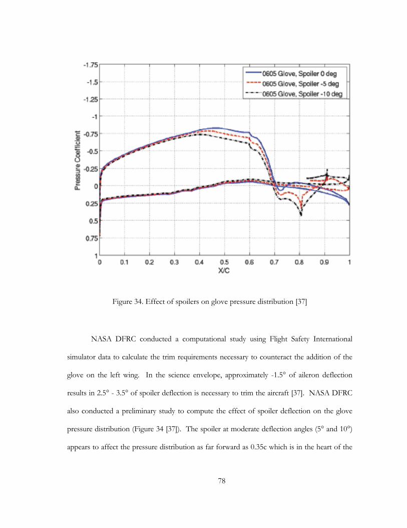
78

NASA DFRC conducted a computational study using Flight Safety International

simulator data to calculate the trim requirements necessary to counteract the addition of the

glove on the left wing. In the science envelope, approximately -1.5° of aileron deflection

results in 2.5° - 3.5° of spoiler deflection is necessary to trim the aircraft [37]. NASA DFRC

also conducted a preliminary study to compute the effect of spoiler deflection on the glove

pressure distribution (Figure 34 [37]). The spoiler at moderate deflection angles (5° and 10°)

appears to affect the pressure distribution as far forward as 0.35c which is in the heart of the

Figure 34. Effect of spoilers on glove pressure distribution [37]

79

glove test section. These spoiler deflection angles equate to aileron deflections of 2.5° and

3.5° which are somewhat large for a stabilized, low-bank angle turn in smooth air. A

computational analysis is needed to simulate the effects of spoiler deflections at [0°, 2°, 5°,

10°, 43° (full deflection)] on the glove test section.

(R 23) Compute the effects of spoiler deflection on the glove test section.

The Gulfstream IIB and III models have a manual reversion mode that depowers the

spoilers by means of the flight power shutoff system. This T-handle is provided on the pilot’s

center pedestal. This T-handle actuates a 6-port hydraulic valve that removes hydraulic

pressure to the flight control actuators and can be reset in flight. The flight power shutoff

system effectively makes the flight spoilers inoperative. However, speedbrakes are then

disabled which are required for emergency descent from high-altitude. Further, manual

reversion carries limits of 250 KIAS and 25,000 ft MSL. Each restriction would prohibit

operation in the science envelope.

(R 24) Do not use the flight power shutoff to disable spoilers for data collection.

Angle of attack data band/tolerances 5.7

The design angle of attack is set during glove design and balances competing

manufacturing and boundary layer stability requirements. Manufacturing considerations drive

the thickness/chord ratio and chordwise extent of the glove on the Gulfstream IIB wing, and

the extent of the glove forward of the Gulfstream IIB forward wing beam.

A glove designer does not have complete freedom to shape the airfoil section but

must remain outside the existing wing airfoil section. Further, the glove position is limited.

80

The inboard extent is limited by fuselage-mounted engine effects [53]. There is also a wing

structure change at the inboard wing section that would complicate glove installation. The

outboard extent of the glove cannot interfere with the flow over the ailerons. The aft section

of the glove cannot interfere with flight spoilers and flaps [3]. Also, there is a practical limit to

the forward extent of the glove due to aerodynamic load and flutter considerations. Finally,

the glove design must allow room for fairings to smoothly transition from the Gulfstream IIB

wing outer mold line (OML) to the glove OML on the inboard, outboard, and aft edges.

The aerodynamic design considerations are peculiar to the research mission of

studying crossflow transition. To this end, streamwise transition (i.e., Tollmien-Schlichting

instability) is suppressed via a favorable pressure gradient throughout the glove test section.

The glove must generate crossflow and is required to have a leading edge sweep, Λ ≥ 30° [3].

Finally, the crossflow instability must become unstable and transition on the glove test

section, 0.15c ≤ tr≤ 0.60c at transport-relevant flight conditions, which is the source of the

science envelope (Figure 15).

The multiple design considerations result in a glove that is designed to operate at a

specific aircraft angle of attack, αtest. The angle of attack planning models are then utilized to

determine if αtest is practicable given the required range of flight conditions in the flight

envelope (Figure 35). The critical consideration is if the Gulfstream IIB can operate at a

single αtest in both the high dynamic pressure flight conditions (i.e., low, fast; 0.75 Mach

number, 27.5M Rec) and low dynamic pressure flight conditions (i.e., high, slow; 0.67 Mach

number, 16.5M Rec). Operations are further restricted by the need for stabilized flight

conditions which are enabled by a bank angle limit, Φlimit = 45° in level flight. The

81

practicability of a given αtest can be evaluated by examining the aircraft angle attack at flight

conditions within the science envelope across the full range of fuel loads (Figure 35).

Examination of Figure 35 shows the balance required to operate at a single design

angle of attack across the entire science envelope. Figure 35a shows that αtest = 3.2° makes all

flight conditions accessible in level flight at angles of bank, 0° ≤ Φ ≤ 45° except the low

dynamic pressure flight condition, 0.67 Mach number, 16.5M Rec. At this flight condition, a

Gulfstream IIB in straight (Φ = 0°), level flight must maintain an angle of attack above αtest.

Figure 35c shows that a glove with αtest = 4.0° can operate at all flight conditions except the

high dynamic pressure flight condition, 0.75 Mach number, 27.5M Rec. At this flight

condition, a Gulfstream IIB with maximum fuel load in level flight requires more than the

limit bank angle, Φlim = 45°, to achieve αtest. The value of αtest = 3.4° balances the requirement

to operate over the entire science envelope.

A word of caution is appropriate here. These angle of attack models are only as good

as the data upon which they rely. Simulator data is currently the only angle of attack data

available, and it is notoriously inaccurate particularly at higher angles of attack and near the

edges of the operational envelope. Therefore, design decisions made on the basis of these

data should consider the source of the data and lean more towards fixing αtest slightly lower.

The importance of this decision early in the design phase also adds impetus to securing flight

data as soon as possible to reduce the uncertainty of the angle of attack model. Nonetheless,

the planning tool indicates the very careful balance necessary to design a glove for a laminar

flow flight experiment.

(R 25) Gather flight data early to reduce the uncertainty of planning decisions.

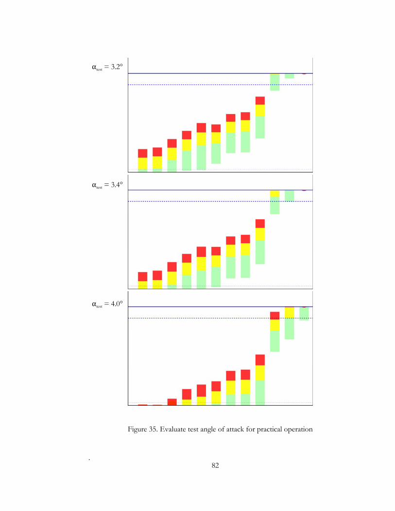
82 .

Figure 35. Evaluate test angle of attack for practical operation

αtest = 3.2°

αtest = 3.4°

αtest = 4.0°

83

Angle of sideslip data band/tolerances 5.8

The angle of sideslip data band is based on the requirement to demonstrate DRE

HLFC effectiveness at leading edge sweep angle, Λ ≥ 30° [3]. Sideslip angles, β > 0° increase

the effective leading edge sweep, Λeff, on the left wing while β < 0° decreases Λeff [54]. In

order to meet the requirement, the amount that Λ exceeds 30° defines the negative β data

band. The positive β data band is not as definite and does not have a test limit in the science

envelope. However, reasonable safety of flight limits should be applied to both positive and

negative angles of sideslip during approach and landing maneuvers and other operations with

a reduced stall margin.

The interaction of the spoilers and aileron inputs tends to favor negative β values.

With a negative beta due to a left turn, dihedral stability, C > 0, indicates that left aileron

input would be required to maintain the bank angle. Right aileron input would move the left

aileron trailing edge down and retract the spoilers.

(R 26) Set the glove leading edge sweep to allow for a reasonable negative β data band.

The angle of sideslip tolerance is based on the requirement for continuous, stabilized

flight data [3]. Based on experience with the O-2A flight research, the angle of sideslip

tolerance, β = 0.1° is a reasonable value. In practice, β is set within the data band with rudder

trim and the test point in flown without further rudder input. The test team monitors the

flow parameters real time to find a 15-sec interval of data that is within tolerances.

84

Mach number 5.9

Mach number tolerances are ± 0.01. This is operationally similar to that required on

North Atlantic Track where no tolerance is allowed [55]. Typically, autothrottles and

autopilot are sufficient to maintain tolerances in smooth air.

Operating limits 5.10

The glove cannot operate in clouds due to atmospheric particles causing loss of

laminar flow and contamination of the instrumentation. Pfenninger suggests that sweep may

be a factor due to spanwise flow and increased time of particle residence in boundary layer

[56]. Aircraft on operational missions encounter clouds 6% of the time [57, 58].

85

6. DESIGNED EXPERIMENT

An experiment is designed to determine the effect of spanwise-periodic discrete

roughness elements (DRE) on glove transition in a random-effects factorial with blocking and

restricted randomization due to practical limitations. Due to the sensitivity of transition

location to angle of attack and the requirement to predetermine the angle of attack data band,

particular attention is given to monitoring the integrity of the angle of attack data collected by

the airdata boom mounted near the glove. Glove pressure distribution and transition location

are evaluated separately as response variables, and transition location with various DRE

configurations is evaluated against natural laminar flow (NLF) transition location as a control.

Two-level factorial designs should be the cornerstone of designed experiments [47].

In this case, DRE configurations (e.g., height, shape, spacing, and surface roughness) are

investigated with a fully randomized 22 factorial with center points in DRE height. Flight

conditions are blocked by sortie and evaluated as a 22 factorial with center points in both

Mach and Reynolds numbers with additional axial points in Mach number.

Angle of attack 6.1

Air data boom alignment is a critical link between the science envelope definition

sorties and the NLF and DRE sorties. It is intended to be permanently installed with the

glove fairings and not affected by a simple change of leading edge configuration. However, to

protect against inadvertent misalignment, a visual check of alignment using marks on the

fuselage is appropriate during preflight and postflight checks (Figure 36). The inspector

would align the top, aft corner of the winglet with the eye position reference on the fuselage

86

then examine the tip of the airdata boom with respect to the alignment marks painted on the

bottom of the fuselage. However, a visual alignment technique will detect only gross

misalignments on the order of degrees. Since the angle of attack databand is expected to be

0.5° to 0.8° and the angle of attack tolerance is ± 0.1°, an inflight check of the airdata boom

alignment is required.

(R 27) Check glove airdata boom alignment during pre/postflight inspections.

A control flight condition can be defined to compare air data boom angle of attack

measurements across sorties for the specific purpose of checking the air data boom alignment

Figure 36. Airdata boom visual alignment marks on the fuselage

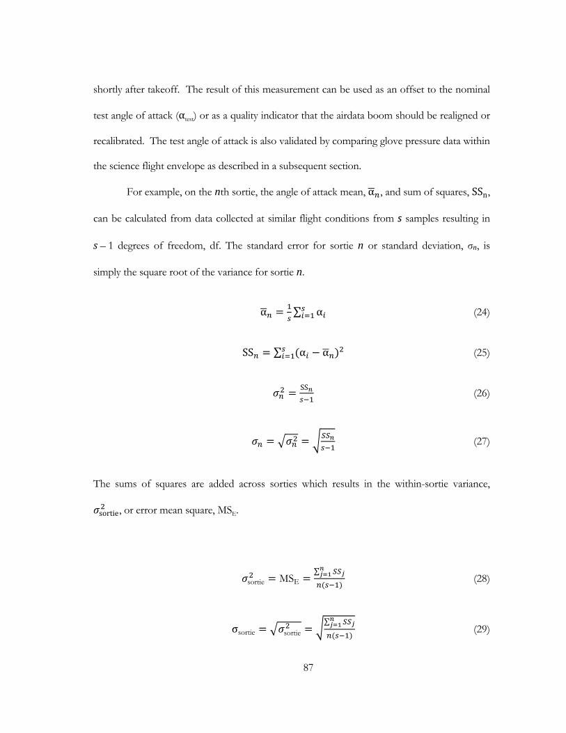
87

shortly after takeoff. The result of this measurement can be used as an offset to the nominal

test angle of attack (αtest) or as a quality indicator that the airdata boom should be realigned or

recalibrated. The test angle of attack is also validated by comparing glove pressure data within

the science flight envelope as described in a subsequent section.

For example, on the nth sortie, the angle of attack mean, α , and sum of squares, SSn,

can be calculated from data collected at similar flight conditions from s samples resulting in

s – 1 degrees of freedom, df. The standard error for sortie n or standard deviation, σn, is

simply the square root of the variance for sortie n.

α ∑ α (24)

SS ∑ α α (25)

SS

(26)

(27)

The sums of squares are added across sorties which results in the within-sortie variance,

sortie, or error mean square, MSE.

sortie MSE∑

(28)

σsortie sortie

∑ (29)

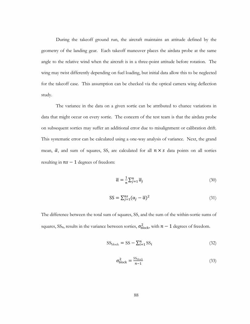
88

During the takeoff ground run, the aircraft maintains an attitude defined by the

geometry of the landing gear. Each takeoff maneuver places the airdata probe at the same

angle to the relative wind when the aircraft is in a three-point attitude before rotation. The

wing may twist differently depending on fuel loading, but initial data allow this to be neglected

for the takeoff case. This assumption can be checked via the optical camera wing deflection

study.

The variance in the data on a given sortie can be attributed to chance variations in

data that might occur on every sortie. The concern of the test team is that the airdata probe

on subsequent sorties may suffer an additional error due to misalignment or calibration drift.

This systematic error can be calculated using a one-way analysis of variance. Next, the grand

mean, , and sum of squares, SS, are calculated for all data points on all sorties

resulting in 1 degrees of freedom:

α ∑ α (30)

SS ∑ α α (31)

The difference between the total sum of squares, SS, and the sum of the within-sortie sums of

squares, SSn, results in the variance between sorties, block, with 1 degrees of freedom.

SSblock SS ∑ SS (32)

blockSSblock (33)

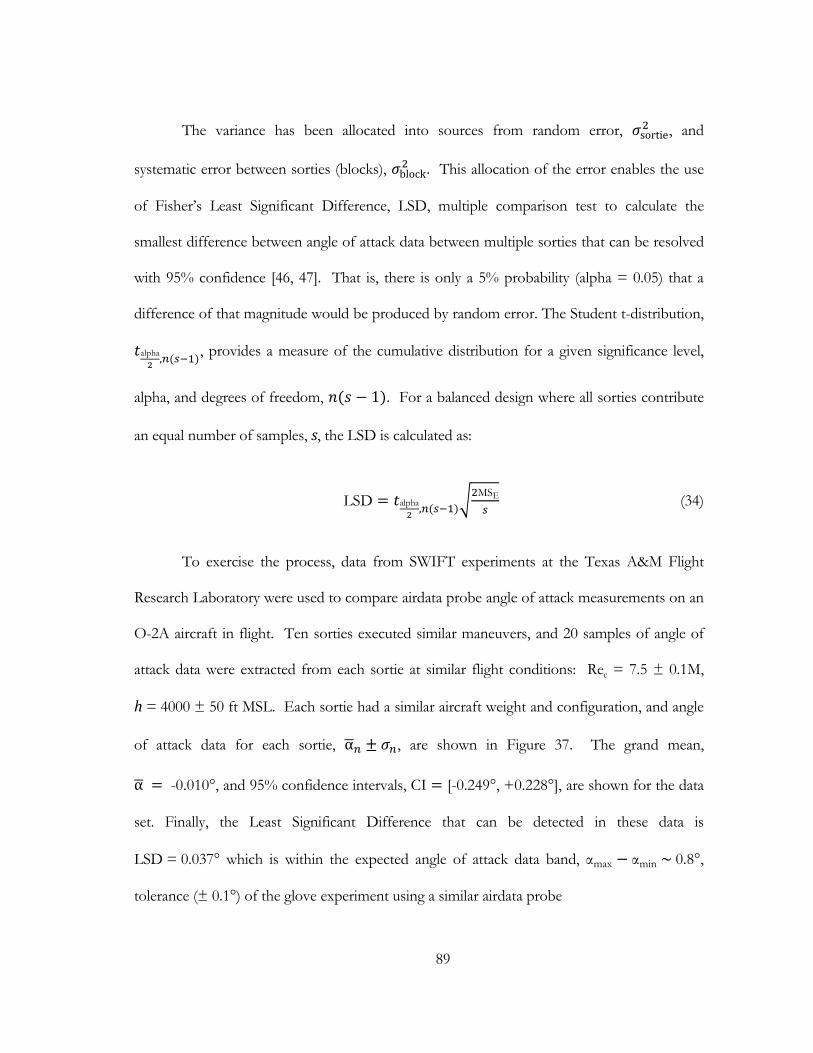
89

The variance has been allocated into sources from random error, sortie, and

systematic error between sorties (blocks), block. This allocation of the error enables the use

of Fisher’s Least Significant Difference, LSD, multiple comparison test to calculate the

smallest difference between angle of attack data between multiple sorties that can be resolved

with 95% confidence [46, 47]. That is, there is only a 5% probability (alpha = 0.05) that a

difference of that magnitude would be produced by random error. The Student t-distribution,

alpha,

, provides a measure of the cumulative distribution for a given significance level,

alpha, and degrees of freedom, 1 . For a balanced design where all sorties contribute

an equal number of samples, s, the LSD is calculated as:

LSD alpha,

MSE (34)

To exercise the process, data from SWIFT experiments at the Texas A&M Flight

Research Laboratory were used to compare airdata probe angle of attack measurements on an

O-2A aircraft in flight. Ten sorties executed similar maneuvers, and 20 samples of angle of

attack data were extracted from each sortie at similar flight conditions: Rec = 7.5 ± 0.1M,

h = 4000 ± 50 ft MSL. Each sortie had a similar aircraft weight and configuration, and angle

of attack data for each sortie, α , are shown in Figure 37. The grand mean,

α -0.010°, and 95% confidence intervals, CI [-0.249°, +0.228°], are shown for the data

set. Finally, the Least Significant Difference that can be detected in these data is

LSD = 0.037° which is within the expected angle of attack data band, αmax αmin~0.8°,

tolerance (± 0.1°) of the glove experiment using a similar airdata probe

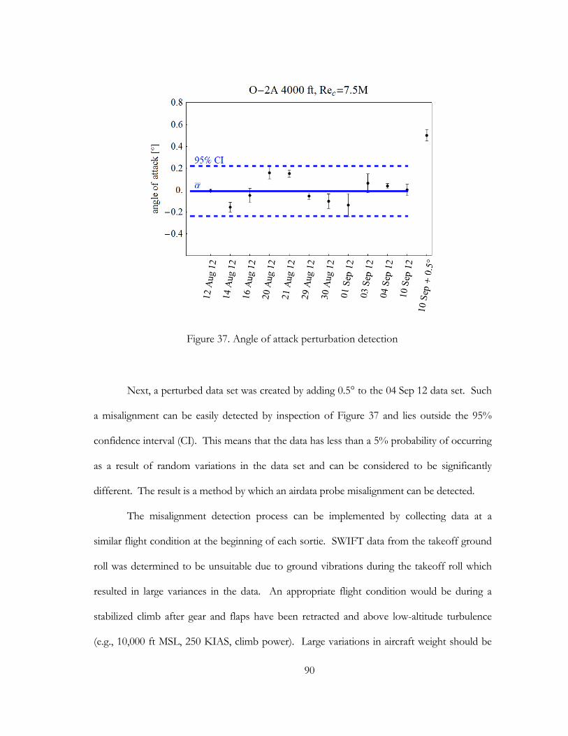
90

Next, a perturbed data set was created by adding 0.5° to the 04 Sep 12 data set. Such

a misalignment can be easily detected by inspection of Figure 37 and lies outside the 95%

confidence interval (CI). This means that the data has less than a 5% probability of occurring

as a result of random variations in the data set and can be considered to be significantly

different. The result is a method by which an airdata probe misalignment can be detected.

The misalignment detection process can be implemented by collecting data at a

similar flight condition at the beginning of each sortie. SWIFT data from the takeoff ground

roll was determined to be unsuitable due to ground vibrations during the takeoff roll which

resulted in large variances in the data. An appropriate flight condition would be during a

stabilized climb after gear and flaps have been retracted and above low-altitude turbulence

(e.g., 10,000 ft MSL, 250 KIAS, climb power). Large variations in aircraft weight should be

Figure 37. Angle of attack perturbation detection

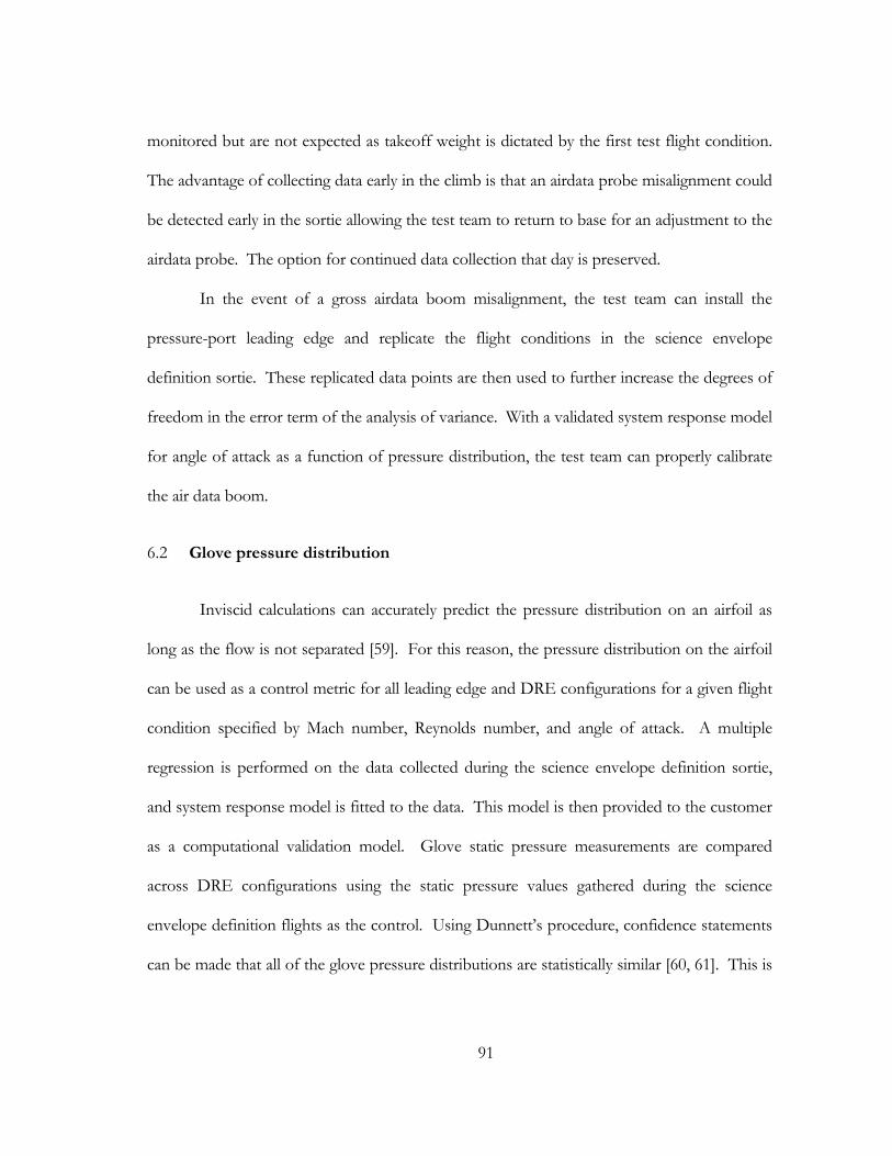
91

monitored but are not expected as takeoff weight is dictated by the first test flight condition.

The advantage of collecting data early in the climb is that an airdata probe misalignment could

be detected early in the sortie allowing the test team to return to base for an adjustment to the

airdata probe. The option for continued data collection that day is preserved.

In the event of a gross airdata boom misalignment, the test team can install the

pressure-port leading edge and replicate the flight conditions in the science envelope

definition sortie. These replicated data points are then used to further increase the degrees of

freedom in the error term of the analysis of variance. With a validated system response model

for angle of attack as a function of pressure distribution, the test team can properly calibrate

the air data boom.

Glove pressure distribution 6.2

Inviscid calculations can accurately predict the pressure distribution on an airfoil as

long as the flow is not separated [59]. For this reason, the pressure distribution on the airfoil

can be used as a control metric for all leading edge and DRE configurations for a given flight

condition specified by Mach number, Reynolds number, and angle of attack. A multiple

regression is performed on the data collected during the science envelope definition sortie,

and system response model is fitted to the data. This model is then provided to the customer

as a computational validation model. Glove static pressure measurements are compared

across DRE configurations using the static pressure values gathered during the science

envelope definition flights as the control. Using Dunnett’s procedure, confidence statements

can be made that all of the glove pressure distributions are statistically similar [60, 61]. This is

92

the basis for the experimental evaluation of the DRE effect on transition location where NLF

is the control.

The test plan benefits in several ways to this technique. First, it relates data collected

using the pressure-port leading edge during the science envelope definition sorties with data

collected without leading edge pressure ports (NLF and DRE sorties). There are two rows of

static pressure ports on the glove (BL 204 and BL264) and each row has 12 static pressure

ports on the suction side and 6 pressure ports on the pressure side. The glove test section

also has two rows of 11 static pressure ports on the pressure side (Figure 38 [36]).

During the science envelope definition sorties, the maximum and minimum angles of

attack (αmin and αmax) were determined by inspecting the pressure distribution of the glove

leading edge and test section pressure port data. The test angle of attack, αtest, is set within

the range (αmin, αmax) which is referenced to the airdata probe near the glove test section.

Figure 38. Glove static pressure ports [36]

93

When the polished and painted leading edges are installed for the NLF and DRE sorties, only

the 11 test section pressure ports are available to compare pressure gradients and values for a

given Mach number, Reynolds number, and angle of attack flight condition across sorties.

The sortie pressure coefficient data from the NLF and DRE sorties are compared to the

control data collected during the science envelope definition sorties.

6.2.1 Science envelope data

The pressure data collected during the science envelope definition sorties will

provide the computational validation model and serve as the control data for the NLF and

DRE sorties. At a specific flight condition, a range of angles of attack are sampled to

produce pressure coefficient data for 15 secs at each angle of attack value each. From this

data set, the pressure coefficient mean, , and variance, , is calculated where m is the

index of the static pressure port in Figure 38.

∑ (35)

SS ∑ (36)

SS

(37)

(38)

Each static pressure port is analyzed separately. During the science envelope

definition sortie, data from all 29 pressure ports will be collected. A system response model

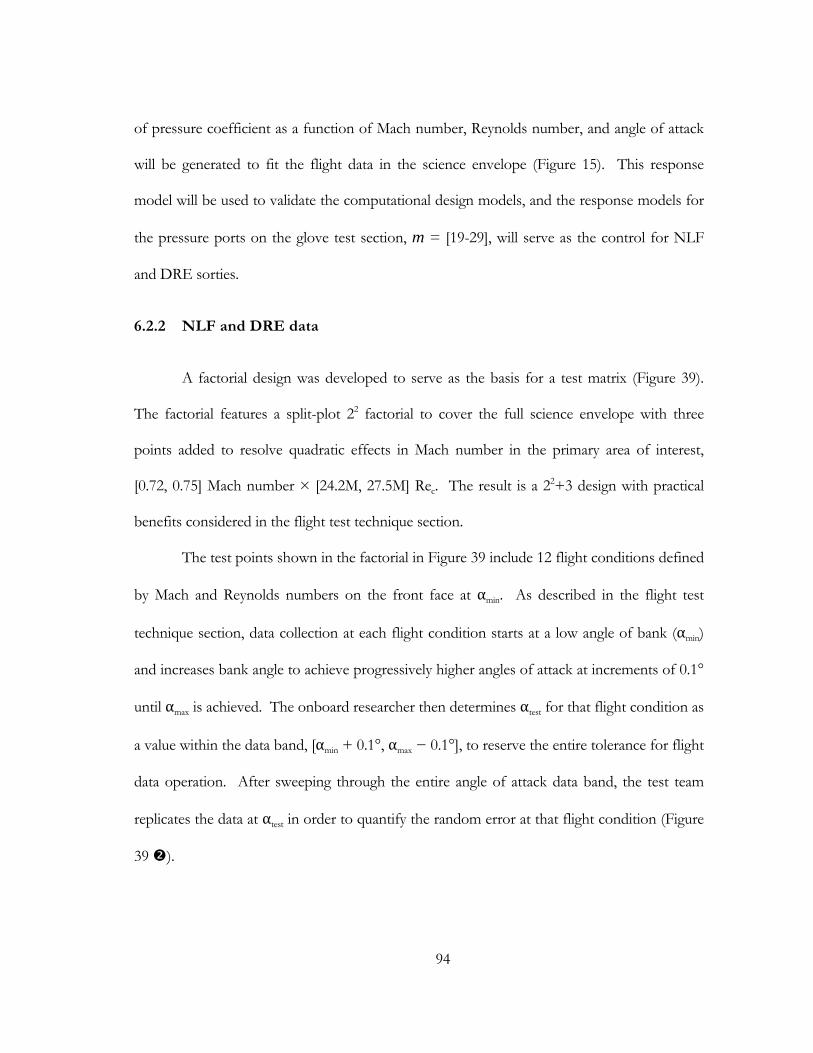
94

of pressure coefficient as a function of Mach number, Reynolds number, and angle of attack

will be generated to fit the flight data in the science envelope (Figure 15). This response

model will be used to validate the computational design models, and the response models for

the pressure ports on the glove test section, m = [19-29], will serve as the control for NLF

and DRE sorties.

6.2.2 NLF and DRE data

A factorial design was developed to serve as the basis for a test matrix (Figure 39).

The factorial features a split-plot 22 factorial to cover the full science envelope with three

points added to resolve quadratic effects in Mach number in the primary area of interest,

[0.72, 0.75] Mach number × [24.2M, 27.5M] Rec. The result is a 22+3 design with practical

benefits considered in the flight test technique section.

The test points shown in the factorial in Figure 39 include 12 flight conditions defined

by Mach and Reynolds numbers on the front face at αmin. As described in the flight test

technique section, data collection at each flight condition starts at a low angle of bank (αmin)

and increases bank angle to achieve progressively higher angles of attack at increments of 0.1°

until αmax is achieved. The onboard researcher then determines αtest for that flight condition as

a value within the data band, [αmin + 0.1°, αmax − 0.1°], to reserve the entire tolerance for flight

data operation. After sweeping through the entire angle of attack data band, the test team

replicates the data at αtest in order to quantify the random error at that flight condition (Figure

39 ).

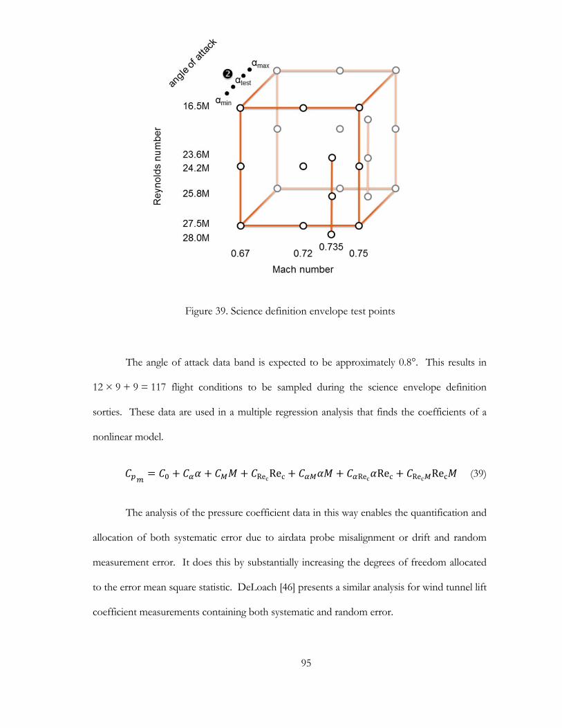
95

The angle of attack data band is expected to be approximately 0.8°. This results in

12 × 9 + 9 = 117 flight conditions to be sampled during the science envelope definition

sorties. These data are used in a multiple regression analysis that finds the coefficients of a

nonlinear model.

RecRec Rec Rec Rec Rec (39)

The analysis of the pressure coefficient data in this way enables the quantification and

allocation of both systematic error due to airdata probe misalignment or drift and random

measurement error. It does this by substantially increasing the degrees of freedom allocated

to the error mean square statistic. DeLoach [46] presents a similar analysis for wind tunnel lift

coefficient measurements containing both systematic and random error.

Figure 39. Science definition envelope test points

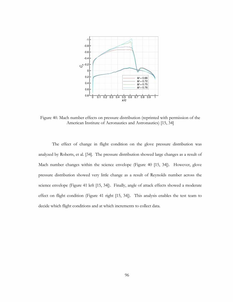
96

The effect of change in flight condition on the glove pressure distribution was

analyzed by Roberts, et al. [34]. The pressure distribution showed large changes as a result of

Mach number changes within the science envelope (Figure 40 [15, 34]). However, glove

pressure distribution showed very little change as a result of Reynolds number across the

science envelope (Figure 41 left [15, 34]). Finally, angle of attack effects showed a moderate

effect on flight condition (Figure 41 right [15, 34]). This analysis enables the test team to

decide which flight conditions and at which increments to collect data.

Figure 40. Mach number effects on pressure distribution (reprinted with permission of the American Institute of Aeronautics and Astronautics) [15, 34]

97

Once the pressure distribution data is collected and analyzed, it is used in a hypothesis

test to support the confidence statement that there is no change in pressure distribution

across science envelope definition, NLF, and DRE sorties. Specifically, n null and alternate

hypotheses are tested where m = [19, 29] pressure ports, j = [0, n] sorties and j = 0 is the

science envelope definition sortie.

:, ,

(40)

:, ,

(41)

The null hypothesis, H0, assumes that there is no significant difference between the

pressure data for ports, m = [19,29], on the glove suction side test section, c = [0.15, 0.60]

(Figure 38). If a significant difference is found between the pressure data on the science

Figure 41. Reynolds number and angle of attack effect on glove pressure distribution (reprinted with permission of the American Institute of Aeronautics and Astronautics)

[15, 34]

98

envelope definition sortie and NLF or DRE sortie, the null hypothesis is rejected.

Significance is set at the type I error rate, alpha = 0.05, so the null hypothesis is rejected with

95% (1 − alpha) confidence. This means that there is a 95% probability that the observed

difference is larger than random error in the data [47].

Each pressure port, m, is compared with the same pressure port data on subsequent

sorties. Dunnett’s procedure is a technique for making multiple comparisons against a

control resulting in a confidence statement where the probability of all n statements being

correct is 95% [60, 61]. First, the computed difference in the pressure means, ,

, is

calculated where m = [19, 29] pressure ports, j = [0, n] sorties and j = 0 is the science

envelope definition sortie.

, ,

(42)

The null hypothesis, H0, is rejected at the type I error rate, alpha = 0.05, when the

pressure data means exceeds the allowance, alpha , 1 , which is referenced with a

two-way comparison table in Dunnett [61] or Montgomery [47]. The tables are organized by

the type I error rate, alpha, number of sorties, n, and the degrees of freedom in the data,

df 1 . If all pressure port data at the same chord location fall within the allowance,

the null hypothesis is not rejected, and the pressure data are not significantly different from

the control pressure data.

, alpha ,df

, , alpha ,df (43)

99

Transition location 6.3

In order to fulfill test objectives and satisfy test requirements, an experiment was

designed to determine the effect of spanwise-periodic, discrete roughness elements (DRE) on

the chordwise transition location, . A split-plot design was used because some variables

can be changed in flight: angle of attack, Mach number, Reynolds number. However, other

variables can only be changed on the ground: DRE height, DRE spacing, and leading edge

roughness [47].

6.3.1 System response model

Transition location data can be analyzed as a system response model where transition

location, , is a function of angle of attack, α, Mach number, M, Reynolds number, Rec,

roughness height, k, DRE spacing, λ, and surface roughness, r. Both Reynolds number and

DRE height are modeled with a second-order term for pure quadratic curvature of the system

response. The split-plot design is blocked by sortie, n, the replicate effect is represented by τ,

and the experimental mean is C.

Interactions are limited to each pair of two variables based on the sparcity of effects

principle. This is the idea that physical systems are based on main effects and low-order

interactions. Interactions between two factors are common, but interactions between three or

more variables are usually negligible in physical systems [47]. Leveraging the sparcity of

effects principle is particularly relevant in experimental designs with low or no replication.

The error associated with higher-order effects is allocated to the error term.

100

A split-plot design cannot be completely randomized, so error is allocated among the

error between DRE configurations, , and random error, . The whole plot main effects and

interactions are tested against : r, k, λ, rk, rλ, kλ, and k2. The subplot main effects and all

other interactions are tested against : α, Rec, M, Rec2, rα, r Rec, rM, kα, k Rec, kM, λα, λ

Rec, λM, α Rec, αM, and Rec M [47].

tr

RecRec Rec Rec Rec Rec Rec

Rec Rec Rec Rec Rec Rec (44)

The analysis of variance allocates 23 degrees of freedom, df, to 23 main effects and

interactions. The error between DRE configurations, , receives t – 1 = 11 df.. Random

error, , receives the remaining 189 degrees of freedom from a total of 208.

6.3.2 Power analysis

The variance has been allocated into sources from random error, treatment, and

systematic error between treatments (blocks), block. This enables the use of Fisher’s Least

Significant Difference, LSD, multiple comparison test to calculate the smallest difference

between transition location data when comparing NLF and DRE configurations that can be

resolved with 95% confidence [46, 47]. For a balanced design where all NLF and DRE

treatments, t, contribute an equal number of flight conditions, s, the LSD is calculated as:

LSD alpha,

MSE (45)

101

6.3.3 Factorials

The experimental design for the transition location is a split-plot factorial [47]. The

subplot is a 22 factorial with a central point and two axial points in Reynolds number that

covers flight conditions on a single sortie and DRE configuration. This factorial represents

each point in the whole plot 23 factorial with center points on the DRE height axis. Both

designs feature partial replication but only the second design is randomized due to practical

limitations on the first.

The subplot is called the flight condition factorial and covers the area of primary

interest in the science envelope to meet the test requirements (Figure 42). The parameter

values, [0.72, 0.75] Mach number × [24.2M, 27.5M] Rec, are all collected at the test angle of

attack, αtest, which can vary from the minimum to the maximum angles of attack defined in

the science envelope definition phase of the test plan. The natural laminar flow investigation

in this parameter range will determine whether or not these parameter values are suitable for

the DRE investigation. In the discussion of the LFC test plan, the NLF sorties measure the

transition location, xtr, and determine which flight conditions will allow a 50% delay in

transition location and remain on the glove surface. Roberts, et al. [34] predicted that this

would occur in the range [24.2M, 27.5M] Rec (Figure 18). Also, when the test conditions

accessible during flight were predicted (Figure 30), a 4.5-hour gap was noted between when

the 0.72 Mach number, 24.2M Rec data could be collected and the availability of the 0.75

Mach number, 16.5M Rec flight condition. The obvious clustering of points in the high-

Mach-number, high-Reynolds-number regime was a compelling reason to set the flight

condition factorial parameters at [0.72, 0.75] Mach number × [24.2M, 27.5M] Rec.

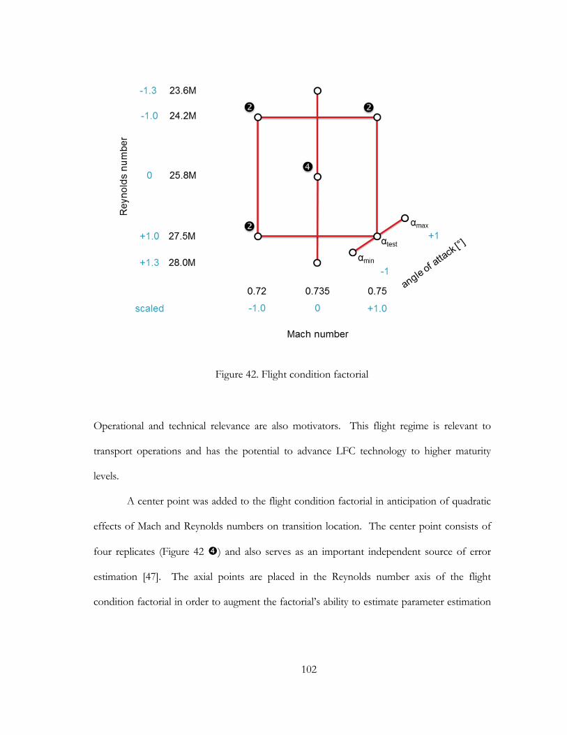
102

Operational and technical relevance are also motivators. This flight regime is relevant to

transport operations and has the potential to advance LFC technology to higher maturity

levels.

A center point was added to the flight condition factorial in anticipation of quadratic

effects of Mach and Reynolds numbers on transition location. The center point consists of

four replicates (Figure 42 ) and also serves as an important independent source of error

estimation [47]. The axial points are placed in the Reynolds number axis of the flight

condition factorial in order to augment the factorial’s ability to estimate parameter estimation

Figure 42. Flight condition factorial

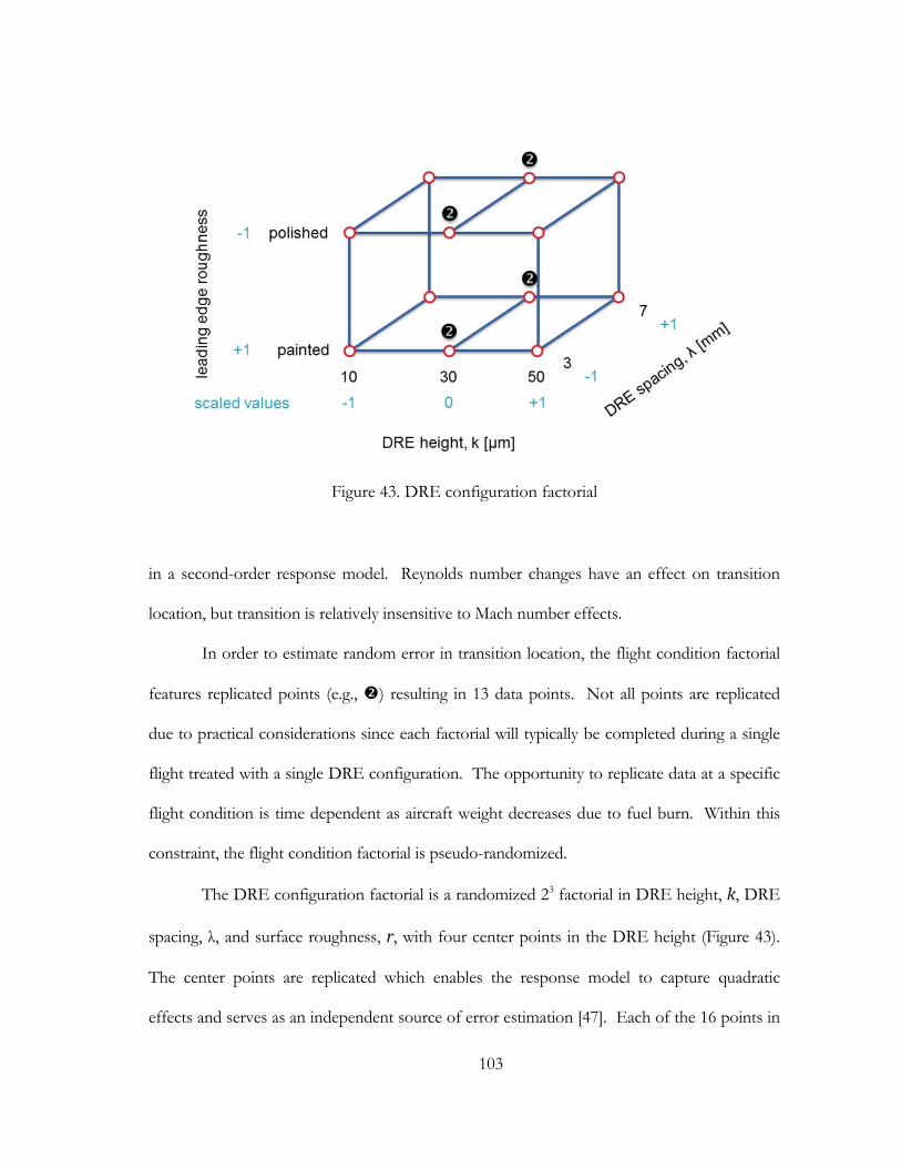
103

in a second-order response model. Reynolds number changes have an effect on transition

location, but transition is relatively insensitive to Mach number effects.

In order to estimate random error in transition location, the flight condition factorial

features replicated points (e.g., ) resulting in 13 data points. Not all points are replicated

due to practical considerations since each factorial will typically be completed during a single

flight treated with a single DRE configuration. The opportunity to replicate data at a specific

flight condition is time dependent as aircraft weight decreases due to fuel burn. Within this

constraint, the flight condition factorial is pseudo-randomized.

The DRE configuration factorial is a randomized 23 factorial in DRE height, k, DRE

spacing, λ, and surface roughness, r, with four center points in the DRE height (Figure 43).

The center points are replicated which enables the response model to capture quadratic

effects and serves as an independent source of error estimation [47]. Each of the 16 points in

Figure 43. DRE configuration factorial

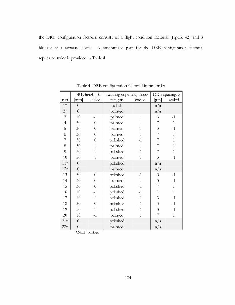
104

the DRE configuration factorial consists of a flight condition factorial (Figure 42) and is

blocked as a separate sortie. A randomized plan for the DRE configuration factorial

replicated twice is provided in Table 4.

Table 4. DRE configuration factorial in run order

DRE height, k Leading edge roughness DRE spacing, λ run [mm] scaled category coded [μm] scaled 1* 0 polish n/a 2* 0 painted n/a 3 10 -1 painted 1 3 -1 4 30 0 painted 1 7 1 5 30 0 painted 1 3 -1 6 30 0 painted 1 7 1 7 30 0 polished -1 7 1 8 50 1 painted 1 7 1 9 50 1 polished -1 7 1 10 50 1 painted 1 3 -1 11* 0 polished n/a 12* 0 painted n/a 13 30 0 polished -1 3 -1 14 30 0 painted 1 3 -1 15 30 0 polished -1 7 1 16 10 -1 polished -1 7 1 17 10 -1 polished -1 3 -1 18 30 0 polished -1 3 -1 19 50 1 polished -1 3 -1 20 10 -1 painted 1 7 1 21* 0 polished n/a 22* 0 painted n/a

*NLF sorties

105

If during the test progression, the NLF transition location for a polished leading edge

is aft of 40% chord location, xtr, NLF > 0.40c, the DRE configuration factorial will collapse to

the painted surface only and be executed as a factorial with 22 + 2 center points.

Alternatively, the leading edge roughness variable could be modified from a categorical to a

quantitative variable. The roughness axis would include two painted leading edges with a

quantitatively different surface roughness height. This change of variables would maintain the

same plan of expenditure of flight test resources. Finally, an additional factor (e.g., DRE

shape, chord location) could be added and the factorial could be replicated. In this event, a

partial factorial is recommended to conserve resources where the additional factor, F, would

be coded with the design generator F = rkλ using the scaled values, -1 and +1, in Table 4.

6.3.4 Hypothesis test

The flight condition factorial is used for both NLF and DRE phases of the test plan.

However, the DRE configuration factorial would not be appropriate for NLF data points

since a zero DRE height, k, and zero DRE spacing, λ, collapse the factorial to simple 2-way

comparison of leading edge roughness categories. Therefore, the NLF and DRE data are

statistically related using Dunnett’s procedure for comparing several treatments with a control

[60, 61]. In this procedure, the six DRE configurations installed on a polished or painted

leading edge are each compared against the corresponding NLF data. The calculated result is

an allowance for which the experimenter can conclude with 95% confidence that all six

comparisons are true.

For a given leading edge roughness, the null hypothesis, H0, assumes that there is no

difference in the mean transition location using only NLF, tr , and a DRE treatment t, tr .

106

: tr tr (46)

The evaluation requirements for DRE performance state that transition must be

delayed at least 50% beyond the transition location demonstrated by NLF only. The first

alternative hypothesis, H1, is a one-way test that reflects the evaluation criterion for a DRE

treatment tand compares the mean transition location, tr , with the control NLF transition

location, tr . However, another alternative hypothesis exists that has value for the

understanding of the physics of the problem. The second alternative hypothesis, H2, assumes

that a change in transition location due to DRE treatment t can be detected.

: tr 1.5 tr (47)

: tr tr (48)

Dunnett’s procedure enables the comparison of each mean transition location, tr ,

resulting from DRE treatment, t, with the NLF control, tr . First, compute the difference

of the treatment means.

tr tr (49)

The null hypothesis, H0, is rejected at the type I error rate, alpha = 0.05, when the

mean transition location data exceeds the allowance, alpha , 1 , which is referenced

with a one-way comparison table in [60] or Montgomery [47]. The tables are organized by the

type I error rate, alpha, number of DRE treatments, t, and the degrees of freedom in the data,

df 1 . If a transition location data point falls outside the allowance, the null

107

hypothesis is rejected, and that DRE treatment is considered significantly different from the

control NLF transition location. The confidence statement for all of the DRE treatments is

made at the (1 − alpha) = 95% confidence level.

tr 1.5 tr alpha ,df (50)

Dunnett [61] recommends setting the ratio of control data points, nc, to treatment

data points, nt, to be approximately equal to the square root of the number of treatments, t.

≅ √ (51)

For t = 12, there should be approximately 3.46 control points. Therefore, three NLF

sorties with each leading edge configuration should be planned for a total of six sorties. This

manner of sampling control data gives the test team the flexibility to compare only the painted

leading edge controls with the painted leading edge DRE treatments ( ≅ √6 2.45) or all

controls and treatments together.

In order to estimate error due to the stability in a process, Montgomery [47]

recommends running replicates in a nonrandom order. In this case, two NLF sorties will

each be equipped with a different leading edge roughness category and flown at the start of

the investigation as shown in Table 4. Collecting NLF transition location data first will give

the test team a sense for transition location when using the polished and painted leading edges

as well as experience with the flight test technique and test procedures. One more NLF sortie

with each of the leading edge roughness conditions should be flown halfway through the

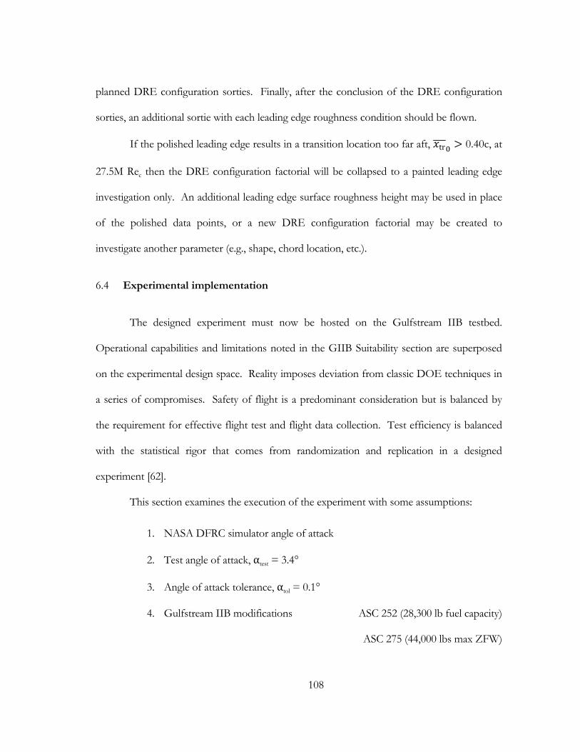
108

planned DRE configuration sorties. Finally, after the conclusion of the DRE configuration

sorties, an additional sortie with each leading edge roughness condition should be flown.

If the polished leading edge results in a transition location too far aft, tr 0.40c, at

27.5M Rec then the DRE configuration factorial will be collapsed to a painted leading edge

investigation only. An additional leading edge surface roughness height may be used in place

of the polished data points, or a new DRE configuration factorial may be created to

investigate another parameter (e.g., shape, chord location, etc.).

Experimental implementation 6.4

The designed experiment must now be hosted on the Gulfstream IIB testbed.

Operational capabilities and limitations noted in the GIIB Suitability section are superposed

on the experimental design space. Reality imposes deviation from classic DOE techniques in

a series of compromises. Safety of flight is a predominant consideration but is balanced by

the requirement for effective flight test and flight data collection. Test efficiency is balanced

with the statistical rigor that comes from randomization and replication in a designed

experiment [62].

This section examines the execution of the experiment with some assumptions:

1. NASA DFRC simulator angle of attack

2. Test angle of attack, αtest = 3.4°

3. Angle of attack tolerance, αtol = 0.1°

4. Gulfstream IIB modifications ASC 252 (28,300 lb fuel capacity)

ASC 275 (44,000 lbs max ZFW)

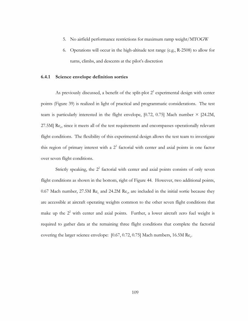
109

5. No airfield performance restrictions for maximum ramp weight/MTOGW

6. Operations will occur in the high-altitude test range (e.g., R-2508) to allow for

turns, climbs, and descents at the pilot’s discretion

6.4.1 Science envelope definition sorties

As previously discussed, a benefit of the split-plot 22 experimental design with center

points (Figure 39) is realized in light of practical and programmatic considerations. The test

team is particularly interested in the flight envelope, [0.72, 0.75] Mach number × [24.2M,

27.5M] Rec, since it meets all of the test requirements and encompasses operationally relevant

flight conditions. The flexibility of this experimental design allows the test team to investigate

this region of primary interest with a 23 factorial with center and axial points in one factor

over seven flight conditions.

Strictly speaking, the 22 factorial with center and axial points consists of only seven

flight conditions as shown in the bottom, right of Figure 44. However, two additional points,

0.67 Mach number, 27.5M Rec and 24.2M Rec, are included in the initial sortie because they

are accessible at aircraft operating weights common to the other seven flight conditions that

make up the 22 with center and axial points. Further, a lower aircraft zero fuel weight is

required to gather data at the remaining three flight conditions that complete the factorial

covering the larger science envelope: [0.67, 0.72, 0.75] Mach numbers, 16.5M Rec.

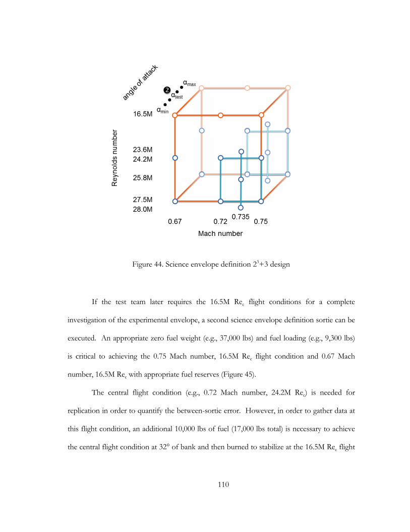
110

If the test team later requires the 16.5M Rec flight conditions for a complete

investigation of the experimental envelope, a second science envelope definition sortie can be

executed. An appropriate zero fuel weight (e.g., 37,000 lbs) and fuel loading (e.g., 9,300 lbs)

is critical to achieving the 0.75 Mach number, 16.5M Rec flight condition and 0.67 Mach

number, 16.5M Rec with appropriate fuel reserves (Figure 45).

The central flight condition (e.g., 0.72 Mach number, 24.2M Rec) is needed for

replication in order to quantify the between-sortie error. However, in order to gather data at

this flight condition, an additional 10,000 lbs of fuel (17,000 lbs total) is necessary to achieve

the central flight condition at 32° of bank and then burned to stabilize at the 16.5M Rec flight

Figure 44. Science envelope definition 23+3 design

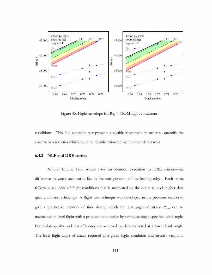
111

conditions. This fuel expenditure represents a sizable investment in order to quantify the

error between sorties which could be reliably estimated by the other data sorties.

6.4.2 NLF and DRE sorties

Natural laminar flow sorties have an identical execution to DRE sorties—the

difference between each sortie lies in the configuration of the leading edge. Each sortie

follows a sequence of flight conditions that is motivated by the desire to seek higher data

quality and test efficiency. A flight test technique was developed in the previous section to

give a practicable window of time during which the test angle of attack, αtest, can be

maintained in level flight with a production autopilot by simply setting a specified bank angle.

Better data quality and test efficiency are achieved by data collected at a lower bank angle.

The level flight angle of attack required at a given flight condition and aircraft weight in

Figure 45. Flight envelope for Rec = 16.5M flight conditions

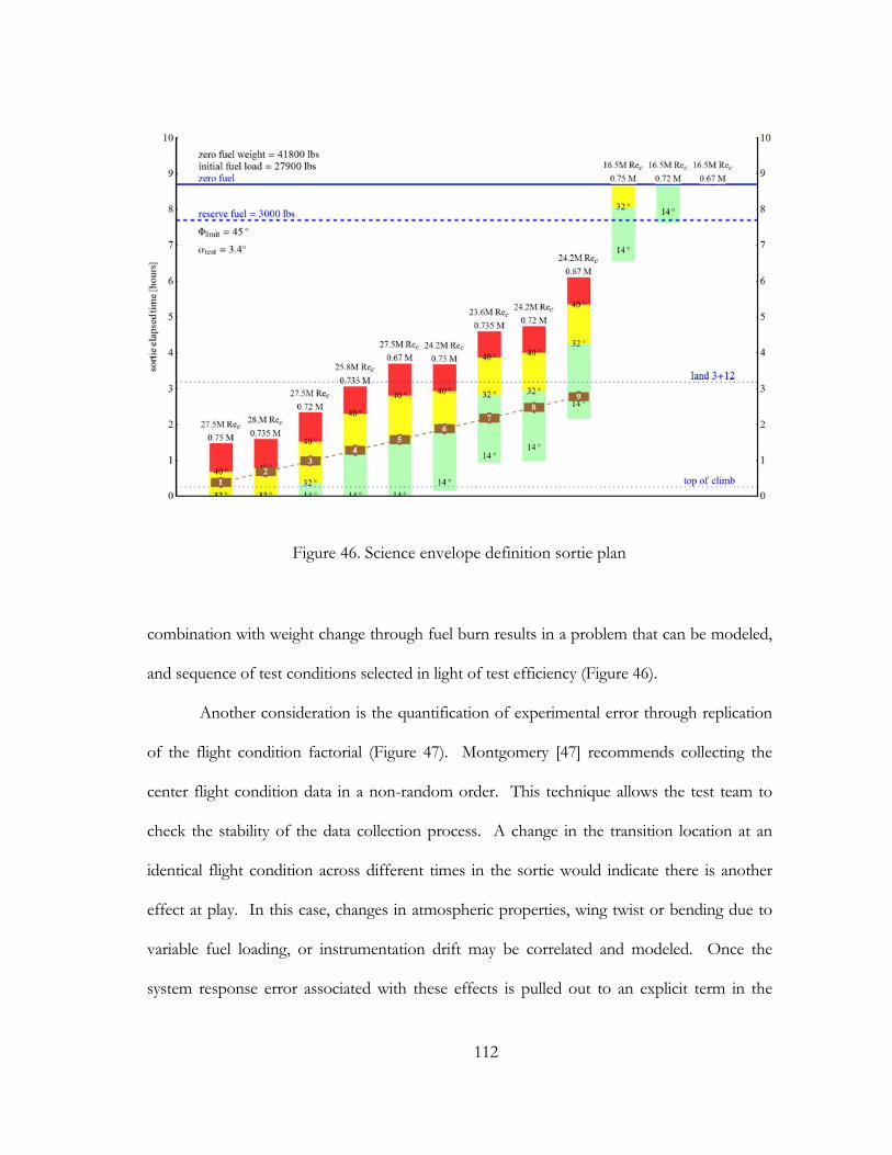
112

combination with weight change through fuel burn results in a problem that can be modeled,

and sequence of test conditions selected in light of test efficiency (Figure 46).

Another consideration is the quantification of experimental error through replication

of the flight condition factorial (Figure 47). Montgomery [47] recommends collecting the

center flight condition data in a non-random order. This technique allows the test team to

check the stability of the data collection process. A change in the transition location at an

identical flight condition across different times in the sortie would indicate there is another

effect at play. In this case, changes in atmospheric properties, wing twist or bending due to

variable fuel loading, or instrumentation drift may be correlated and modeled. Once the

system response error associated with these effects is pulled out to an explicit term in the

Figure 46. Science envelope definition sortie plan

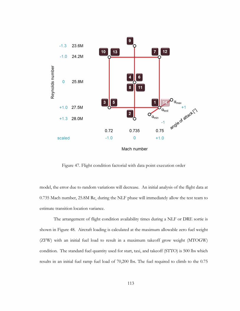
113

model, the error due to random variations will decrease. An initial analysis of the flight data at

0.735 Mach number, 25.8M Rec during the NLF phase will immediately allow the test team to

estimate transition location variance.

The arrangement of flight condition availability times during a NLF or DRE sortie is

shown in Figure 48. Aircraft loading is calculated at the maximum allowable zero fuel weight

(ZFW) with an initial fuel load to result in a maximum takeoff grow weight (MTOGW)

condition. The standard fuel quantity used for start, taxi, and takeoff (STTO) is 500 lbs which

results in an initial fuel ramp fuel load of 70,200 lbs. The fuel required to climb to the 0.75

Figure 47. Flight condition factorial with data point execution order

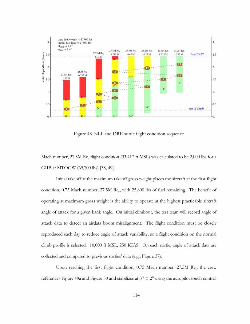
114

Mach number, 27.5M Rec flight condition (33,417 ft MSL) was calculated to be 2,000 lbs for a

GIIB at MTOGW (69,700 lbs) [38, 49].

Initial takeoff at the maximum takeoff gross weight places the aircraft at the first flight

condition, 0.75 Mach number, 27.5M Rec, with 25,800 lbs of fuel remaining. The benefit of

operating at maximum gross weight is the ability to operate at the highest practicable aircraft

angle of attack for a given bank angle. On initial climbout, the test team will record angle of

attack data to detect an airdata boom misalignment. The flight condition must be closely

reproduced each day to reduce angle of attack variability, so a flight condition on the normal

climb profile is selected: 10,000 ft MSL, 250 KIAS. On each sortie, angle of attack data are

collected and compared to previous sorties’ data (e.g., Figure 37).

Upon reaching the first flight condition, 0.75 Mach number, 27.5M Rec, the crew

references Figure 49a and Figure 50 and stabilizes at 37 ± 2° using the autopilot touch control

Figure 48. NLF and DRE sortie flight condition sequence

115

steering. The pilot stabilizes on and maintains flight conditions within tolerances using power

inputs to control Mach number, rudder trim to control angle of sideslip, and autopilot touch

control steering to control model angle of attack. The onboard researcher monitors the flow

conditions at the glove airdata boom and calls the test point complete when 15 secs of

continuous data are recorded. Approximately six minutes of flight time are estimated to be

sufficient to gather these data, and three minutes is estimated to change flight conditions.

This is possible due to the similar energy states of the flight conditions that make up the NLF

and DRE factorials.

In order to preserve the orthogonal properties of the flight condition factorial and

simplify the analysis, Montgomery [47] recommends estimating missing replicates if only a

few are missing. In the flight condition factorial, practical limitations prevented more than

one replicate at 0.75 Mach number, 27.5M Rec. To estimate the missing data point (14 in

Figure 47), the average of the differences for the other replicated main effects would be

added.

The progression of flight conditions laid out in Figure 48 is annotated in the

appropriate flight condition chart of Figure 49 with bank angle deviations annotated in Figure

50. When executing the DRE factorial (Figure 51), the first 22 sorties are projected in Table

4. Each sortie duration is estimated at 2.5 hours, so the initial investigation of DRE

configurations will take 55 flight hours.

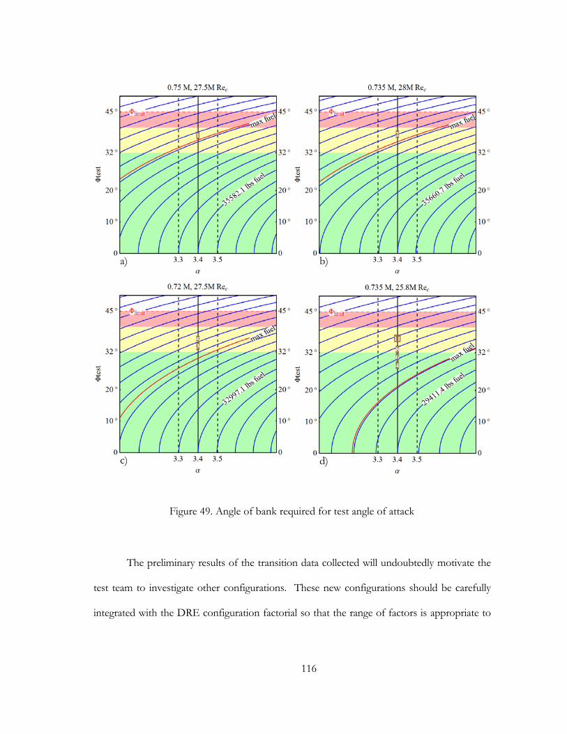
116

The preliminary results of the transition data collected will undoubtedly motivate the

test team to investigate other configurations. These new configurations should be carefully

integrated with the DRE configuration factorial so that the range of factors is appropriate to

Figure 49. Angle of bank required for test angle of attack

d)c)

b)a)

117

the scientific investigation [63]. The balance of the funded flight hours can then be efficiently

used to fully investigate the experimental space.

Figure 49 (Continued)

d)g)

f)e)

118

Figure 51. DRE configuration factorial with data point execution order

Figure 50. Allowable change in test angle of bank

119

7. SUMMARY AND RECOMMENDATIONS

This success of a DRE LFC flight research program depends on the ability of the test

team to meet the test objectives. A properly developed test plan and a practical flight test

technique are critical to the success of the test program. The original contributions of this

work specified a test plan using a build-up approach to gather data in the appropriate order

for test efficiency, efficacy, and safety. A novel flight test technique was developed that

recognizes the challenge in gathering flight data that is very sensitive to very small changes in

angle of attack. The flight test technique also balances the angle of attack data band with the

tolerances required to produce very precise data for computational validation. In order to

predict the suitability of a Gulfstream IIB aircraft, an analytic model was produced to assess

the practicability of the glove design for the current flight experiment. The glove design angle

of attack appears to be suitable for the Gulfstream IIB operating in the science envelope.

From this analytic model, planning tools were produced to guide safe, effective, and efficient

test execution. Finally, an experiment was designed to statistically analyze the flight data and

draw conclusions on the effect of the DRE HLFC flight experiment and compare the data to

the test requirements.

The recommendations are sorted by importance and tabulated with page numbers.

Flight safety recommendations:

(R 1) Periodically fly the pressure-port leading edge to ensure valid glove flow conditions. .................................................................................................................................. 34 

(R 2) Monitor test section pressure ports for changes with reference to test angle of attack. ........................................................................................................................................... 34 

120

(R 3) Develop procedures to avoid contact with the airdata boom during ground operations. .................................................................................................................................. 34 

(R 4) Make turns to the right to keep left spoiler from deploying. ................................................ 48 

(R 5) Plan data collection at Φ ≤ 32° as much as possible. ............................................................ 50 

(R 6) Set maximum bank angle, Φlimit = 45° to enable autopilot use for all data points. ........... 50 

(R 7) Use only smooth, slow throttle movements in the science envelope. ................................ 51 

(R 8) Install the pilot display so as to not block aircraft control instruments. ............................. 54 

(R 9) Generate the pilot display using a dedicated processor. ........................................................ 54 

(R 10) Provide portable oxygen bottles for the research crew. ...................................................... 55 

(R 11) Ensure aircraft oxygen supply is sufficient to operate above 41,000 ft MSL. ................. 55 

(R 12) Provide a separate intercom circuit for the research crew. ................................................. 56 

(R 13) Develop a communication plan for the test team. ............................................................... 56 

(R 14) Develop coordinated normal and emergency checklists for the test team. ..................... 56 

(R 15) Provide functional onboard lavatory facilities for the crew. ............................................... 57 

(R 16) Provide a life raft for the crew if operating over water for extended periods of time. ............................................................................................................................................. 57 

(R 17) Use multi-layered fuel reserves balance risk mitigation and the research mission. ....................................................................................................................................... 70 

(R 18) Monitor flow conditions real time to select continuous, stabilized data for analysis. ........................................................................................................................................ 75 

(R 19) Schedule sorties just after sunrise during stable weather conditions. ................................ 75 

(R 20) Measure the spoiler deflection as a function of aileron input on the test aircraft. ......... 77 

(R 21) Adjust aileron input/spoiler deflection deadband to maximum allowable. ..................... 77 

(R 22) Use optical targets to determine spoiler deflection during test point execution. ............ 77 

(R 23) Compute the effects of spoiler deflection on the glove test section. ................................ 79 

(R 24) Do not use the flight power shutoff to disable spoilers for data collection. ................... 79 

121

(R 25) Gather flight data early to reduce the uncertainty of planning decisions. ........................ 81 

(R 26) Set the glove leading edge sweep to allow for a reasonable negative β data band. ............................................................................................................................................ 83 

(R 27) Check glove airdata boom alignment during pre/postflight inspections. ........................ 86 

122

REFERENCES

1. Saric, W. S., Reed, H. L., and White, E. B., "Stability and Transition of Three-Dimensional Boundary Layers," Annual Review of Fluid Mechanics, no. 35, 2003, pp. 413-40. doi: 10.1146/annurev.fluid.35.101101.161045

2. Bezos-O'Connor, G. M., Maglesdorf, M. F., Maliska, H. A., Washburn, A. E., and Wahls, R. A., "Fuel Efficiencies Through Airframe Improvements," American Institute of Aeronautics and Astronautics (AIAA) 2011-3530, 2011.

3. "Subsonic Aircraft Roughness Glove Experiment (SARGE) Objectives and Requirements Document (ORD) & Levels I & II System Requirements Specification (SRS)," 804-ORD-101-1.00, Dryden Flight Research Center, Edwards, California, 2011.

4. Marec, J.-P., "Drag Reduction: a Major Task for Research," CEAS/DragNet European Drag Reduction Conference, Potsdam, Germany, 2000, pp. 17-28.

5. Hefner, J. N., "Overview of the Langley Viscous Drag Program," Langley Symposium on Aerodynamics, NASA, Hampton, Virginia, 1985, pp. 393-399.

6. Arcara, P. C., Jr., Bartlett, D. W., and McCullers, L. A., "Analysis for the Application of Hybrid Laminar Flow Control to a Long-Range Subsonic Transport Aircraft," Society of Automotive Engineers (SAE) 912113, 1991.

7. Roeder, J. P., "Laminar Flow Application - Past Realities and Future Prospects," 2nd European Forum on Laminar Flow Technology, Bordeaux, France, 1996, pp. 1.1-1.12.

8. "Fiscal Year (FY) 2011 Budget Estimates, Operations and Maintenance volume I," SAF/FM, Department of the Air Force, 2012.

9. Horton, G., "Forecasts of CO2 Emissions from Civil Aircraft for IPCC," QinetiQ, DTI 06/2178, Farnborogh, England, 2006.

10. Hefner, J. N., and Bushnell, D. M., "An Overview of Concepts for Aircraft Drag Reduction," Special Course on Concepts for Drag Reduction, AGARD-R-654, North Atlantic Treaty Organization Advisory Group for Aerospace Research and Development (NATO RTO), von Kármán Institute, Rhode St. Genèse, Belgium, 1977.

11. Arnal, D., and Archambaud, J. P., "Laminar-Turbulent Transition Control: NLF, LFC, HLFC," AVT-151 RTO AVT/VKI Lecture Series, AC/323(AVIT-151)TP/278, von Kármán Institute, Rhode St. Genèse, Belgium, 2008.

123

12. Saric, W. S., Carpenter, A. L., and Reed, H. L., "Passive Control of Transition in Three-dimensional Boundary Layers, with Emphasis on Discrete Roughness Elements," Philosophical Transactions of the Royal Society vol. 369, 2011, pp. 1352-1364. doi: 10.1098/rsta.2010.0368

13. Saric, W. S., "Introduction to Linear Stability," AVT/VKI Lecture Series, AC/323(AVIT-151)TP/278, NATO RTO, von Kármán Institute, Rhode St. Genèse, Belgium, 2008.

14. Reed, H. L., and Saric, W. S., "Linear Stability Theory Applied to Boundary Layers," Annual Review of Fluid Mechanics vol. 28, 1996, pp. 389-428.

15. Roberts, M. W., "Computational Evaluation of a Transonic Laminar-Flow Wing Glove Design," Master of Science Thesis, Aerospace Engineering, Texas A&M University, College Station, Texas, 2012.

16. Deyhle, H., and Bippes, H., "Disturbance Growth in an Unstable Three-dimensional Boundary Layer and Its Dependence on Environmental Conditions," Journal of Fluid Mechanics vol. 316, 1996, pp. 73-113.

17. Carpenter, A. L., "In-flight Receptivity Experiments on a 30-degree Swept Wing Using Micron-sized Discrete Roughness Elements," Doctor of Philosophy Dissertation, Aerospace Engineering, Texas A&M University, College Station, TX, 2009.

18. Hunt, L. E., and Saric, W. S., "Boundary-Layer Receptivity of Three-Dimensional Roughness Arrays on a Swept Wing," American Institute of Aeronautics and Astronautics (AIAA) 2011-3881, 2011.

19. Joslin, R. D., "Overview of Laminar Flow Control," NASA/TP-1998-208705, Langley Research Center, Hampton, Virginia, 1998.

20. Collier, F. S., Jr., "An Overview of Recent Subsonic Laminar Flow Control Flight Experiments," American Institute of Aeronautics and Astronautics (AIAA) 93-2987, 1993.

21. Zalovcik, J. A., "A Profile-drag Investigation in Flight on an Experimental Fighter-type Airplane - The North American XP-51 (Air Corps Serial No. 41-38)," National Advisory Committee for Aeronautics, ACR 245, Langley Field, Virginia, 1942.

22. Pfenninger, W., "Laminar Flow Control: Laminarization," Special Course on Concepts for Drag Reduction. vol. AGARD-R-654, North Atlantic Treaty Organization Advisory Group for Aerospace Research and Development (NATO RTO), von Kármán Institute, Rhode St. Genèse, Belgium, 1977.

124

23. Edwards, B., "Laminar Flow Control - Concepts, Experiences, Speculations," Special Course on Concepts for Drag Reduction. vol. AGARD-R-654, North Atlantic Treaty Organization Advisory Group for Aerospace Research and Development (NATO RTO), von Kármán Insitute, Rhode St. Genèse, Belgium, 1977.

24. Maddalon, D. V., and Braslow, A. L., "Simulated-Airline-Service Flight Tests of Laminar Flow Control with Perforated Surface Suction System," NASA TP-2966, Langley Research Center, Hampton, Virginia, 1990.

25. Voogt, N., "Flight Testing of a Fokker 100 Test Aircraft with Laminar Flow Glove," 2nd European Forum on Laminar Flow Technology, Bordeaux, France, 1996, pp. 2.3-2.14.

26. Bolsunovsky, A., Buzoverya, N., Kotscheev, A., Cheryemukhin, G., Shapiro, A., et al., "The Tu-22M Flying Test Bed for Laminar Flow Studies," 2nd European Forum on Laminar Flow Technology, Bordeaux, France, 1996, pp. 2.15-2.18.

27. Rhodes, R. G., Carpenter, A. L., Reed, H. L., and Saric, W. S., "CFD Analysis of Flight-Test Configuration for LFC on Swept Wings," American Institute of Aeronautics and Astronautics (AIAA) 2008-7336, 2008.

28. Rhodes, R. G., Reed, H. L., Saric, W. S., Carpenter, A. L., and Neale, T. P., "Roughness Receptivity in Swept-wing Boundary Layers-Computations," International Journal of Engineering Systems Modelling and Simulation vol. 2, no. 1/2, 2010, pp. 139-148. doi: 10.1504/IJESMS.2010.031878

29. Martin, M. L., Carpenter, A. L., and Saric, W. S., "Swept-Wing Laminar Flow Control Studies Using Cessna O-2A Test Aircraft," American Institute of Aeronautics and Astronautics (AIAA) 2008-1636, 2008.

30. Saric, W. S., Carpenter, A. L., Hunt, L. E., McKnight, C., and Schouten, S., "SWIFT Safety Analysis for Swept-Wing Experiments," Texas A&M University, TAMUS-AE-TR-06-002, revision B, College Station, Texas, 2007.

31. "Flying Qualities of Piloted Airplanes," Department of Defense, Military Specification (MIL)-F-8785C, 1980.

32. Belisle, M. J., Roberts, M. W., Tufts, M. W., Tucker, A. A., Williams, T. C., et al., "Design of the Subsonic Aircraft Roughness Glove Experiment (SARGE)," American Institute of Aeronautics and Astronautics (AIAA) 2011-3524, 2011.

33. Belisle, M. J., Roberts, M. W., Williams, T. C., Tufts, M. W., Tucker, A. A., et al., "A Transonic Laminar-Flow Wing Glove Flight Experiment: Overview and Design Optimization," American Institute of Aeronautics and Astronautics (AIAA) 2012-2667, 2012.

125

34. Roberts, M. W., Reed, H. L., and Saric, W. S., "A Transonic Laminar-Flow Wing Glove Flight Experiment: Computational Evaluation and Linear Stability," American Institute of Aeronautics and Astronautics (AIAA) 2012-2668, 2012.

35. Drake, A., and Solomon, W. D., Jr.,, "Flight Testing of a 30-degree Sweep Laminar Flow Wing for a High-Altitude Long-Endurance Aircraft," American Institute of Aeronautics and Astronautics (AIAA) 2010-4571, 2010.

36. Williams, T. C., "Design of an Instrumentation System for a Boundary Layer Transition Wing Glove Experiment," Master of Science Thesis, Aerospace Engineering, Texas A&M University, College Station, Texas, 2012.

37. "DRE Laminar Flow Glove Experiment Preliminary Design Review," National Aeronautics and Space Administration, Dryden Flight Research Center, Edwards, California, 2012.

38. "Gulfstream IIB Flight Manual," Gulfstream American Corporation, Savannah, Georgia, 1981.

39. "Type Certificate no. A12EA," Federal Aviation Administration, Department of Transportation, 1997.

40. "Gulfstream IIB Upgrades," Jane's Aircraft Upgrades 2013, Jane's All the World's Aircraft (2011), https://janes.ihs.com/CustomPages/Janes/DisplayPage.aspx?DocType=Reference&ItemId=+++1337442, accessed on 02 Oct 12.

41. "C-20A Flight Manual," Gulfstream Aerospace Corporation, TO 1C-20A-1, Savannah, Georgia, 2004.

42. "Flying Qualities Testing," Air Force Flight Test Center, US Air Force, Edwards Air Force Base, California, 2003.

43. Diamond, W. J., Practical Experiment Designs for Engineers and Scientists. 3rd ed. New York: John Wiley & Sons, Inc., 2001.

44. Smith, W., "Autopilot Specs," personal correspondance to Tucker, A. A., 17 Aug 12.

45. Mathematica version 8.0, Wolfram Research, Inc., Champaign, Illinois, www.wolfram.com/mathematica, 2010.

46. DeLoach, R., "Analysis of Variance in the Modern Design of Experiments," American Institute of Aeronautics and Astronautics (AIAA) 2010-1111, 2010.

47. Montgomery, D. C., Design and Analysis of Experiments. 6th ed. Hoboken, New Jersey: John Wiley & Sons, Inc., 2005.

126

48. "Independent Review of the ERA Airframe Technology Subproject DRE Laminar Flow Glove Experiment," Dryden Flight Research Center, Edwards, California, 2011.

49. "Gulfstream III Cruise Control Manual," Gulfstream American Corporation, Savannah, Georgia, 1985.

50. "Gulfstream II," Jane's Aircraft Upgrades 2013, Jane's All the World's Aircraft (2011), https://janes.ihs.com/CustomPages/Janes/DisplayPage.aspx?DocType=Reference&ItemId=+++1337443, accessed on 02 Oct 12.

51. "Gulfstream III," Jane's Aircraft Upgrades 2013, Jane's All the World's Aircraft (2011), https://janes.ihs.com/CustomPages/Janes/DisplayPage.aspx?DocType=Reference&ItemId=+++1337446, accessed on 02 Oct 12.

52. Idicula, J., "Gulfstream III Roll Performance Study," Dryden Flight Research Center, Edwards, California, 2010.

53. Belisle, M. J., Neale, T. P., Reed, H. L., and Saric, W. S., "Design of a Swept-Wing Laminar Flow Control Flight Experiment for Transonic Aircraft," American Institute of Aeronautics and Astronautics (AIAA) 2010-4381, 2010.

54. Nelson, R. C., Flight Stability and Automatic Control. New York: McGraw-Hill, Inc., 1989.

55. "Guidance Concerning Air Navigation In and Above the North Atlantic MNPS Airspace," European and North Atlantic Office of International Civil Aviation Organization, NAT Doc 007, North Atlantic Systems Planning Group, 2010.

56. Fisher, D., Horstmann, K. H., and Reidel, H., "Flight Test Measurement Techniques for Laminar Flow," North Atlantic Treaty Organization Advisory Group for Aerospace Research and Development (NATO RTO), AC/323(SCI-040)TP/45, 2003.

57. Jasperson, W. H., Nastrom, G. D., Davis, R. E., and Holderman, J. D., "GASP Cloud-Encounter Statistics: Implications for Laminar Flow Control Flight," AIAA Journal of Aircraft vol. 21, no. 11, 1984, pp. 851-857.

58. Snyder, J. L., "Effect of Clouds in LFC Applications," Research and Technology Division, Research Report AD454476, Systems Engineering Group, Wright-Patterson Air Force Base, Ohio, 1964.

59. Anderson, J. D., Jr., Fundamentals of Aerodynamics. New York: McGraw-Hill, Inc., 1991.

60. Dunnett, C. W., "A Multiple Comparison Procedure for Comparing Several Treatments with a Control," Journal of the American Statistical Association vol. 50, no. 272, 1955, pp. 1096-1121.

127

61. Dunnett, C. W., "New Tables for Multiple Comparisons with a Control," Biometrics vol. 20, no. 3, 1964, pp. 482-491.

62. Tucker, A. A., "Safety, Efficacy, and Efficiency: Design of Experiments in Flight Test," 56th Annual Society of Experimental Test Pilots Symposium, Society of Experimental Test Pilots, Anaheim, Calffornia, 2012.

63. Box, G. E. P., Hunter, W. G., and Hunter, J. S., Statistics for Experimenters. New York: John Wiley & Sons, 1978.

128

APPENDIX

MATHEMATICA SCRIPTS

129

The script was written in Mathematica 8.0 and should be executed sequentially in

order to place the variables in the kernel.

A.1. Script for standard atmosphere

ClearAll[w,,,h,M,fuel,T,p,,a,U,q]; (*Standard Atmosphere*) =1.4; R=287;(*m2/s2/K*) s=1.7894*^-5; (*kg/m/s*) g0=9.806; (*m/s^2*) ps=101325; (*Pa*) a1m=-6.5*^-3; (*K/m*) a1ft=-1.9812*^-3; (*K/ft*) Ts=288.16; (*K*) T1=a1ft h+Ts/.h36089 ;(*K*) p1=ps (T1/Ts)^(-g0/(a1m R)); (*Pa*) T[h_]:=Piecewise[{{a1ft h+Ts,0h<36089},{T1,36089h<82021}}];(*T in K, h in ft*) p[h_]:=Piecewise[{{ps (T[h]/Ts)^(-g0/(a1m R)),0h<36089},{p1 Exp[-g0/R 2.54*^-2 12(h-36089)/T[h]],36089h<82021}}];(*T in K, h in ft, p in Pa*) [h_]:=p[h]/(R T[h]);(*kg/m3*) [h_]:=s (T[h]/Ts)^1.5(Ts+110)/(T[h]+110);(*kg/m/s*)

130

A.2. Script for Figure 28. Angle of attack model residue plot

(*level,flight,angle,of,attack*) ClearAll[CM,CW,Ch,W,M,h,model,data]; (*W[lb],M,h[ft],[°]*) data=_{{43970,0.75,22500,0.136},{46940,0.75,22500,0.401},{49910,0.75,22500,0.606},{52880,0.75,22500,0.774},{55850,0.75,22500,0.941},{58820,0.75,22500,1.131},{61790,0.75,22500,1.329},{64760,0.75,22500,1.512},{67730,0.75,22500,1.608},{43970,0.66,30000,1.45},{46940,0.66,30000,1.68},{49910,0.66,30000,1.89},{52880,0.66,30000,2.11},{55850,0.66,30000,2.37},{58820,0.66,30000,2.63},{61790,0.66,30000,2.9},{64760,0.66,30000,3.14},{67730,0.66,30000,3.35},{70700,0.66,30000,3.55},{43970,0.71,37000,1.8},{46940,0.71,37000,2.05},{49910,0.71,37000,2.37},{52880,0.71,37000,2.69},{55850,0.71,37000,3.02},{58820,0.71,37000,3.3},{61790,0.71,37000,3.56},{64760,0.71,37000,3.78},{67730,0.71,37000,3.98},{70700,0.71,37000,4.2},{43970,0.75,40000,1.754},{46940,0.75,40000,1.994},{49910,0.75,40000,2.296},{52880,0.75,40000,2.606},{55850,0.75,40000,2.928},{58820,0.75,40000,3.214},{61790,0.75,40000,3.485},{64760,0.75,40000,3.703},{67730,0.75,40000,3.908},{43970,0.76,40000,1.68},{46940,0.76,40000,1.93},{49910,0.76,40000,2.23},{52880,0.76,40000,2.54},{55850,0.76,40000,2.88},{58820,0.76,40000,3.18},{61790,0.76,40000,3.45},{64760,0.76,40000,3.68},{67730,0.76,40000,3.89},{70700,0.76,40000,4.1},{43970,0.76,44000,2.47},{46940,0.76,44000,2.89},{49910,0.76,44000,3.26},{52880,0.76,44000,3.59},{55850,0.76,44000,3.87},{58820,0.76,44000,4.15},{61790,0.76,44000,4.43},{64760,0.76,44000,4.71},{67730,0.76,44000,4.96},{70700,0.76,44000,5.33}}; Dimensions[data]; level=NonlinearModelFit[data,c0+cW W +cW2 W^2+ch2 h^2 +cWh W h+cWM W M+chM h M,{c0,cW,cW2,ch2,cWh,cWM,chM},{W,M,h}] Normal[level]; level["BestFitParameters"] level["ParameterTable"] level["AdjustedRSquared"] level["FitResiduals"] level["ParameterConfidenceIntervals"]; level["ANOVATable"] var=Sqrt[level["EstimatedVariance"]] Needs["PlotLegends`"]

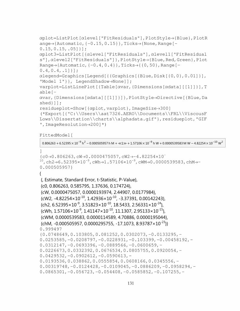
131

plot=ListPlot[level["FitResiduals"],PlotStyle{Blue},PlotRange{Automatic,{-0.15,0.15}},Ticks{None,Range[-0.15,0.15,.05]}]; plot3=ListPlot[{level["FitResiduals"],level1["FitResiduals"],level2["FitResiduals"]},PlotStyle{Blue,Red,Green},PlotRange{Automatic,{-0.4,0.4}},Ticks{{0,50},Range[-0.4,0.4,.1]}]; legend=Graphics[Legend[{{Graphics[{Blue,Disk[{0,0},0.01]}],"Model 1"}}, LegendShadowNone]]; varplot=ListLinePlot[{Table[var,{Dimensions[data][[1]]}],Table[-var,{Dimensions[data][[1]]}]},PlotStyleDirective[{Blue,Dashed}]]; residueplot=Show[{plot,varplot},ImageSize300] (*Export[{"C:\\Users\\aat7326.AERO\\Documents\\FRL\\ViscousFLows\\Dissertation\\charts\\alphadata.gif"},residueplot,"GIF",ImageResolution200]*) FittedModel[

] {c00.806263,cW0.0000475057,cW2-4.82254×10-10,ch26.52395×10-9,cWh1.57106×10-9,cWM0.0000539583,chM-0.000505957} { {, Estimate, Standard Error, t-Statistic, P-Value}, {c0, 0.806263, 0.585795, 1.37636, 0.174724}, {cW, 0.0000475057, 0.0000193974, 2.44907, 0.0177984}, {cW2, -4.82254×10-10, 1.42936×10-10, -3.37391, 0.00142243}, {ch2, 6.52395×10-9, 3.51823×10-10, 18.5433, 2.56331×10-24}, {cWh, 1.57106×10-9, 1.41147×10-10, 11.1307, 2.95133×10-15}, {cWM, 0.0000539583, 0.0000114589, 4.70886, 0.0000195044}, {chM, -0.000505957, 0.0000295755, -17.1073, 8.93787×10-23}} 0.999497 {0.0748649,0.103805,0.081252,0.0302073,-0.0133295,-0.0253585,-0.0208797,-0.0228931,-0.103399,-0.00458192,-0.0312147,-0.0693396,-0.0889566,-0.0600659,-0.0226673,0.0332392,0.0676534,0.0805755,0.0920054,-0.0429532,-0.0902612,-0.0590613,-0.0193536,0.038862,0.0555854,0.0608166,0.0345556,-0.00319748,-0.0124428,-0.0109045,-0.0886209,-0.0958294,-0.0865301,-0.056723,-0.054408,-0.0585852,-0.107255,-

0.806263 + 6.52395μ 10-9 h2 - 0.000505957 h M +á1à+ 1.57106μ 10-9 h W + 0.0000539583 M W - 4.82254μ 10-10 W2

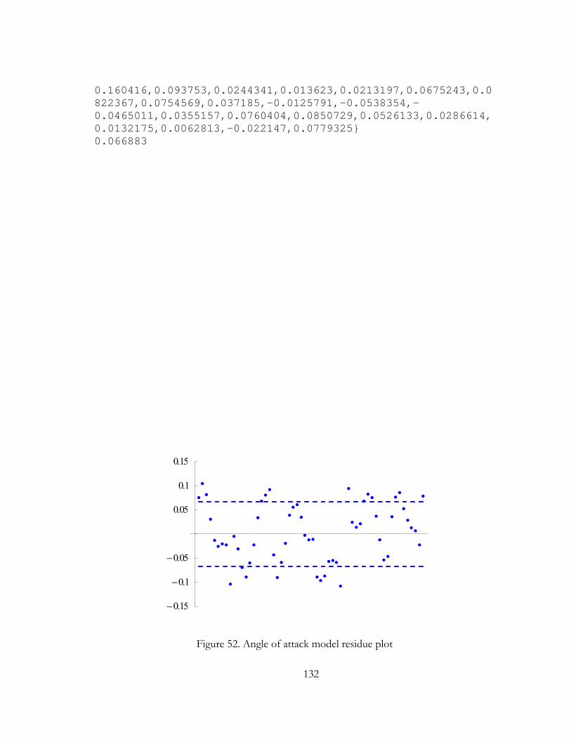
132

0.160416,0.093753,0.0244341,0.013623,0.0213197,0.0675243,0.0822367,0.0754569,0.037185,-0.0125791,-0.0538354,-0.0465011,0.0355157,0.0760404,0.0850729,0.0526133,0.0286614,0.0132175,0.0062813,-0.022147,0.0779325} 0.066883

-0.15

-0.1

-0.05

0.05

0.1

0.15

Figure 52. Angle of attack model residue plot

133

A.3. Script for Figure 27. Simulator angle of attack data

a[h_]:=Sqrt[ R T[h]](*m/s*) U[h_,M_]:=M a[h](*m/s*) q[h_,M_]:=0.5[h] U[h,M]^2(*Pa*) Rec[h_,M_]:=[h]U[h,M]c/[h] (*Reynolds number based on glove chord*) (*constants*) c=4.41706; (*glove chord [m]*) S=86.83;(*m^2*) Cl=1.589 Pi;(*/rad*) test=3.4;(*deg*) ZFW=41900;(*lb 44000 lbs max*) weightmin=ZFW+fuelmin; weightmax=69700; fuelmin=3000; (*lbs*) fuelmax=28300;(*lbs 27900 without ASC 252 increased fuel modification, 28300 with ASC 252*) fuelmaxtest=fuelmax-fuelclimb; (*fuel remaining to start testing*) fuelinit=12000; (*initial fuel load*) fullfuel=If[weightmax-ZFW>fuelmax,fuelmax,weightmax-ZFW]; (*lbs*) fuelclimb=2000; (*70000 TOGW, ISA+10°C, 33500 ft initial leveloff = 2000 lbs fuel, 15.5 mins*) timeclimb=0.258; (*hrs*) timedescend=17/60; (*hrs*) opt=14°;(*deg*) lim=45°;(*deg*) hmin=29000;(*ft*) hmax=45000;(*ft*) Mmin=0.65; Mmax=0.77; testMachlist={.67,.72,.75}; testRelist={16.5*^6,24.2*^6,27.5*^6}; centerpoint={{25.8*^6,0.735},{28.0*^6,0.735},{23.6*^6,0.735}}; banklist={0,10°,20°,32°,40°,lim}; op=0.3; fuelt[t_]:=fullfuel-Piecewise[{{7750t,0t<.258},{2000+3300(t-

134

0.258),0.258t<1},{4450+3200(t-1),1t<2},{7650+3150(t-2),2t<3},{10800+3000(t-3),3t}}]; (*lbs*) (*create lists of test points*) fltcond=Table[{testRe,testM},{testRe,testRelist},{testM,testMachlist}]; fltcondcp=Join[fltcond,{centerpoint}]; testpoints=Flatten[Table[{testmach,h/.FindRoot[Rec[h,testmach]testRe,{h,10000}]},{testmach,testMachlist},{testRe,testRelist}],1]; testpointcp=Flatten[{Table[{centerpoint[[i,2]],h/.FindRoot[Rec[h,centerpoint[[i,2]]]centerpoint[[i,1]],{h,10000}]},{i,3}]},1]; testpointcp=Join[testpoints,testpointcp]; (*calculate endurance at reserve fuel and zero fuel*) enduranceres=t/.FindRoot[fuelt[t]fuelmin,{t,0.5}]//N; (*hrs*) endurancezero=t/.FindRoot[fuelt[t]0,{t,0.5}]//N ;(*hrs*) (*calculate Mach number and altitude at test Reynolds numbers for label placement*) Re1h=h/.FindRoot[Rec[h,Mmin]testRelist[[1]],{h,hmin}]; Re1M=M/.FindRoot[Rec[hmin,M]testRelist[[1]],{M,Mmin}]; Re2h=h/.FindRoot[Rec[h,Mmin]testRelist[[2]],{h,hmin}]; Re2M=M/.FindRoot[Rec[hmin,M]testRelist[[2]],{M,Mmin}]; Re3h=h/.FindRoot[Rec[h,Mmin]testRelist[[3]],{h,hmin}]; Re3M=M/.FindRoot[Rec[hmin,M]testRelist[[3]],{M,Mmin}]; Re1label=Graphics[Text[Style["16.5M",FontSizeSmall,BackgroundWhite,Gray],{If[Re1h hmax,Mmin,Re1M],If[Re1hhmax,Re1h,hmax]},{-1,0}]]; Re2label=Graphics[Text[Style["24.2M",FontSizeSmall,BackgroundWhite,Gray],{If[Re2h hmax,Mmin,Re2M],If[Re2hhmax,Re2h,hmax]},{-1,0}]]; Re3label=Graphics[Text[Style["27.5M",FontSizeSmall,BackgroundWhite,Gray],{If[Re3h hmax,Mmin,Re3M],If[Re3hhmax,Re3h,hmax]},{-1,0}]]; Relabel=Graphics[Text[Style["Rec",FontSizeSmall,BackgroundWhite,Gray],{If[Re1h hmax,Mmin,Re1M],If[Re1hhmax,Re1h,hmax]},{-1,-2}]]; Replot=ContourPlot[{Rec[h,M]testRelist[[1]],Rec[h,M]testRelist[[2]],Rec[h,M]testRelist[[3]]},{M,Mmin,Mmax},{h,hmin,hmax},ContourStyleDirective[Gray,Dashing[Tiny]]]; Replot=Show[Replot,Relabel,Re1label,Re2label,Re3label];

135

hoffset=2200; Moffset=0.002; (*create a 3D list plot*) Re1label3D=Graphics3D[Text[Style["16.5M",FontSizeSmall,BackgroundWhite,Gray],{If[Re1h hmax,Mmin+Moffset,Re1M],If[Re1hhmax,Re1h,hmax],weightmin}]]; Re2label3D=Graphics3D[Text[Style["24.2M",FontSizeSmall,BackgroundWhite,Gray],{If[Re2h hmax,Mmin+Moffset,Re2M],If[Re2hhmax,Re2h,hmax],weightmin}]]; Re3label3D=Graphics3D[Text[Style["27.5M",FontSizeSmall,BackgroundWhite,Gray],{If[Re3h hmax,Mmin+Moffset,Re3M],If[Re3hhmax,Re3h,hmax],weightmin}]]; Relabel3D=Graphics3D[Text[Style["Rec",FontSizeSmall,BackgroundWhite,Gray],{If[Re1h hmax,Mmin+Moffset,Re1M],If[Re1hhmax,Re1h+hoffset,hmax],weightmin}]]; Relist=Flatten[Table[{testmach,h/.FindRoot[Rec[h,testmach]testRe,{h,10000}]},{testRe,testRelist},{testmach,Mmin,Mmax,0.002}],1]; weightminarray=ConstantArray[weightmin,{Dimensions[Relist][[1]],1}]; Relistweight=Join[Relist,weightminarray,2]; Relistplot=ListPointPlot3D[Relistweight,PlotStyleDirective[Gray,PointSize[Small],Opacity[0.9]]]; Relistplot=Show[Relistplot,Re1label3D,Re2label3D,Re3label3D,Relabel3D]; (*plot fuel burn curve*) Plot[fuelt[t],{t,0,endurancezero}, PlotRange{0,fuelmax}] wtt[t_]:=ZFW+fuelt[t]; (*weight as a function of time*) wt[fuel_]:=ZFW+fuel; (*constant weight*) (*define angle of attack as a function of bank angle, fuel weight, Mach number, altitude, time*) bank[_,fuel_,M_,h_]:=level[wt[fuel],M,h]/Cos[]; bankt[_,M_,h_,t_]:=level[wtt[t],M,h]/Cos[]; fltcond=Join[data[[All,2;;3]],Transpose[{data[[All,1]]}],2]; weightminarray=ConstantArray[weightmin,{Dimensions[testpoints][[1]],1}];

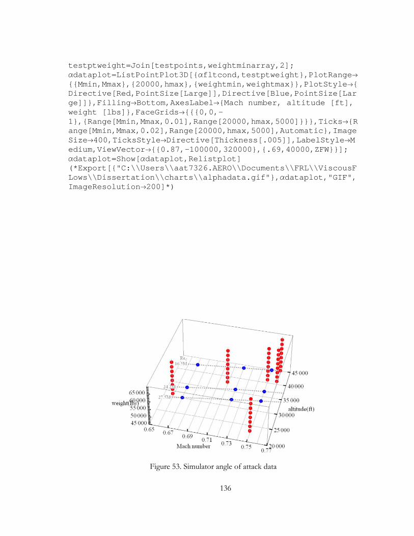
136

testptweight=Join[testpoints,weightminarray,2]; dataplot=ListPointPlot3D[{fltcond,testptweight},PlotRange{{Mmin,Mmax},{20000,hmax},{weightmin,weightmax}},PlotStyle{Directive[Red,PointSize[Large]],Directive[Blue,PointSize[Large]]},FillingBottom,AxesLabel{Mach number, altitude [ft], weight [lbs]},FaceGrids{{{0,0,-1},{Range[Mmin,Mmax,0.01],Range[20000,hmax,5000]}}},Ticks{Range[Mmin,Mmax,0.02],Range[20000,hmax,5000],Automatic},ImageSize400,TicksStyleDirective[Thickness[.005]],LabelStyleMedium,ViewVector{{0.87,-100000,320000},{.69,40000,ZFW}}]; dataplot=Show[dataplot,Relistplot] (*Export[{"C:\\Users\\aat7326.AERO\\Documents\\FRL\\ViscousFLows\\Dissertation\\charts\\alphadata.gif"},dataplot,"GIF",ImageResolution200]*)

Figure 53. Simulator angle of attack data

137

A.4. Script for Figure 30. Test conditions accessible during flight

(*solve for the fuel weight(given in sortie elapsed time at which a given bank angle, Mach number, and Reynolds number produce the aircraft angle of attack equal to the test angle of attack*) endurancefindbase=0.01; fltcondtlevel=Table[{t/.FindRoot[bankt[0,testM,h/.FindRoot[Rec[h,testM]testRe,{h,20000}],t]test,{t,5,endurancefindbase,endurancezero+1}]},{testRe,testRelist},{testM,testMachlist}]; fltcondtopt=Table[{t/.FindRoot[bankt[opt,testM,h/.FindRoot[Rec[h,testM]testRe,{h,20000}],t]test,{t,5,endurancefindbase,endurancezero+1}]},{testRe,testRelist},{testM,testMachlist}]; fltcondt20=Table[{t/.FindRoot[bankt[20°,testM,h/.FindRoot[Rec[h,testM]testRe,{h,20000}],t]test,{t,5,endurancefindbase,endurancezero+1}]},{testRe,testRelist},{testM,testMachlist}]; fltcondt32=Table[{t/.FindRoot[bankt[32°,testM,h/.FindRoot[Rec[h,testM]testRe,{h,20000}],t]test,{t,5,endurancefindbase,endurancezero+1}]},{testRe,testRelist},{testM,testMachlist}]; fltcondt40=Table[{t/.FindRoot[bankt[40°,testM,h/.FindRoot[Rec[h,testM]testRe,{h,20000}],t]test,{t,5,endurancefindbase,endurancezero+1}]},{testRe,testRelist},{testM,testMachlist}]; fltcondtbanklim=Table[{t/.FindRoot[bankt[lim,testM,h/.FindRoot[Rec[h,testM]testRe,{h,20000}],t]test,{t,5,endurancefindbase,endurancezero+1}]},{testRe,testRelist},{testM,testMachlist}]; centerendure=Table[{t/.FindRoot[bankt[bank,centerpoint[[i,2]],h/.FindRoot[Rec[h,centerpoint[[i,2]]]centerpoint[[i,1]],{h,20000}],t]test,{t,5,endurancefindbase,endurancezero+1}]},{i,3},{bank,banklist}]; centerendure=Join[centerpoint,Partition[Flatten[centerendure],6],2]; fltcondfull=Join[Flatten[Join[fltcond,fltcondtlevel,fltcondtopt,fltcondt20,fltcondt32,fltcondt40,fltcondtbanklim,3],1],centerendure]; numfltcond=Dimensions[fltcondfull][[1]]; numfltcondt=Dimensions[fltcondfull][[2]]; fltcondt=Sort[fltcondfull,#1[[7]]<#2[[7]]&];

138

fltcondt//Grid endurelevel=Table[fltcondt[[i]][[3]],{i,1,numfltcond}]; endureopt=Table[fltcondt[[i]][[4]],{i,1,numfltcond}]; endure20=Table[fltcondt[[i]][[5]],{i,1,numfltcond}]; endure32=Table[fltcondt[[i]][[6]],{i,1,numfltcond}]; endure40=Table[fltcondt[[i]][[7]],{i,1,numfltcond}]; endurebanklim=Table[fltcondt[[i]][[-1]],{i,1,numfltcond}];

139

Table 5. Endurance data for flight conditions

Rec Mach 0° 14° 20° 32° 40° 45° 2.75 10 0.75 0.01 0.01 0.01 0.01 0.68224 1.47702.8 10 0.735 0.01 0.01 0.01 0.01 0.77761 1.59872.75 10 0.72 0.01 0.01 0.01 0.3652 1.5242 2.34332.58 10 0.735 0.01 0.01 0.1488 1.2272 2.3071 3.06912.75 10 0.67 0.01 0.0149 0.2224 1.5866 2.8131 3.69512.42 10 0.75 0.1486 0.3823 0.7694 1.9226 2.9363 3.67672.36 10 0.735 0.9263 1.1199 1.6944 2.8390 3.8715 4.59852.42 10 0.72 0.9735 1.3653 1.7641 2.9389 4.0009 4.74402.42 10 0.67 2.1640 2.5745 2.9907 4.2595 5.3497 6.10951.65 10 0.75 6.559 6.8592 7.1659 8.0704 8.8628 9.42301.65 10 0.72 7.6314 7.9311 8.2374 9.1408 9.6666 9.66661.65 10 0.67 9.3024 9.6026 9.6666 9.6666 9.6666 9.6666

(*endurance plot*) (*zero, reserve, climb fuel lines*) endureresplot=ListLinePlot[{{0,enduranceres},{numfltcond+1,enduranceres}},PlotStyle{Dashed,Blue,Thick,Opacity[0.9]},FrameTrue]; endurezeroplot=ListLinePlot[{{0,endurancezero},{numfltcond+1,endurancezero}},PlotStyle{Blue,Thick,Opacity[0.9]},FrameTrue]; climbplot=ListLinePlot[{{0,timeclimb},{numfltcond+1,timeclimb}},PlotStyle{Blue,Dotted,Opacity[.8]},FrameTrue]; reservelabel=Graphics[Text[Style["reserve fuel = "<>ToString[fuelmin]<>" lbs",Blue,Thick,Medium],{.5,enduranceres},{-1,-1}]]; endurelabel=Graphics[Text[Style["zero fuel",Blue,Thick,Medium],{.5,endurancezero},{-1,-1}]]; climblabel=Graphics[Text[Style["top of climb",Blue,Thick,Medium],{numfltcond+.5,timeclimb},{1,-1}]]; (*labels for constants*) limitlabel=Graphics[Text[Style["limit = "<>ToString[lim,StandardForm],Thick,Medium],{.5,enduranceres},{-1,2}]]; testlabel=Graphics[Text[Style["test = "<>ToString[test]<>"°",Thick,Medium],{.5,enduranceres},{-1,5}]]; fullfuellabel=Graphics[Text[Style["initial fuel load = "<>ToString[fullfuel]<>" lbs",Thick,Medium],{.5,endurancezero},{-1,-3.0}]];

140

ZFWlabel=Graphics[Text[Style["zero fuel weight = "<>ToString[ZFW]<>" lbs",Thick, Medium],{.5,endurancezero},{-1,-5.0}]]; (*labels for flight condition bars*) fltcondticklabel=Graphics[Text[StringForm["`1`M Rec `2` M",fltcondt[[1]][[1]]/10^6//EngineeringForm,fltcondt[[1]][[2]]//StandardForm]]]; fltcondlabel=Table[{Graphics[Text[Style[StringForm["`1`M Rec `2` M",fltcondt[[i]][[1]]/10^6//EngineeringForm,fltcondt[[i]][[2]]],BackgroundDirective[White]],{i,If[endurebanklim[[i]]endurancezero,endurebanklim[[i]],endurancezero]},{0,-1}]]},{i,1,numfltcond}]; blocks=Graphics[{White,Rectangle[{10.8,endurancezero},{11.2,Ceiling[endurancezero+1]}],Rectangle[{11.8,endurancezero},{12.2,Ceiling[endurancezero+1]}]}]; (*endurance chart*) fltcondlistplot=ListPlot[{endurelevel,endureopt,endure20,endure32,endure40,endurebanklim},FillingStyleDirective[Thickness[.04],Opacity[0.5]],Filling{1{{4},Directive[Green,Thickness[.04],CapForm["Butt"],Opacity[op]]},4{{5},Directive[Yellow,Thickness[.04],CapForm["Butt"],Opacity[0.9]]},5 {{6},Directive[Red,Thickness[.04],CapForm["Butt"],Opacity[0.8]]}},PlotRange{{0,numfltcond+1},{0,Ceiling[endurancezero]}},PlotRangeClippingTrue,PlotMarkers{"","14°","","32°","40°",""},Frame{{1,1},{1,0}},FrameLabel{None,"sortie elapsed time [hours]"},PlotRangePadding{{Automatic,Automatic},{Automatic,1}},PlotStyleBlack,FrameTicks{{Join[Range[0,Ceiling[endurancezero+1]]],Join[Range[0,Ceiling[endurancezero+1]]]},{None,None}}]; testptplanplot=Show[fltcondlistplot,blocks,climbplot,endureresplot,endurezeroplot,reservelabel,endurelabel,limitlabel,fullfuellabel,ZFWlabel,testlabel,fltcondlabel,climblabel,ImageSize700,FrameStyleDirective[Thickness[.002]],TicksStyleDirective[Thickness[.002]],LabelStyleMedium] (*Export[{"C:\\Users\\aat7326.AERO\\Documents\\FRL\\ViscousFLows\\Dissertation\\charts\\testpointop"<>ToString[test]<>"_"<>ToString[ZFW]<>"_"<>ToString[fullfuel]<>".gif"},testptplanplot,"GIF",ImageResolution200]*)

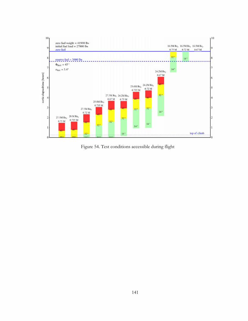
141

Figure 54. Test conditions accessible during flight

142

A.5. Script for Figure 48. NLF and DRE sortie flight condition sequence

(*test point order for endurance chart*) testptplan=(_{ {1, .75, 27.5*^6, 1, 0, 0, 0, 0, 0}, {2, .735, 28.0*^6, 2, 0, 0, 0, 0, 0}, {3, .72, 27.5*^6, 3, 0, 0, 0, 0, 0}, {4, .735, 25.8*^6, 4, 0, 0, 0, 0, 0}, {5, .72, 27.5*^6, 3, 0, 0, 0, 0, 0}, {6, .735, 25.8*^6, 4, 0, 0, 0, 0, 0}, {7, .75, 24.2*^6, 6, 0, 0, 0, 0, 0}, {8, .735, 25.8*^6, 4, 0, 0, 0, 0, 0}, {9, .735, 23.6*^6, 7, 0, 0, 0, 0, 0}, {10, .72, 24.2*^6, 8, 0, 0, 0, 0, 0}, {11, .735, 25.8*^6, 4, 0, 0, 0, 0, 0}, {12, .75, 24.2*^6, 6, 0, 0, 0, 0, 0}, {13, .72, 24.2*^6, 8, 0, 0, 0, 0, 0} }_); testptdur=6/60; (*time to complete a test point*) testptinter=3/60; (*time to transition between test points*) numtestpts=Dimensions[testptplan][[1]]; testptplan[[;;,5]]=(testptplan[[;;,1]]-1)*(testptdur+testptinter)+timeclimb;(*time at beginning of test point*) testptplan[[;;,6]]=testptplan[[;;,5]]+testptdur; (*time at end of test point*) testptplan[[;;,7]]=testptplan[[;;,5]]+testptdur/2; (*put the label in the middle*) timeland=testptplan[[numtestpts,6]]+timedescend; (*calculate the landing time*) fueldescend=fuelt[testptplan[[numtestpts,6]]]; descendlabel=Graphics[Text[Style["top of descent",Blue,Thick,Medium],{numfltcond+.5,testptplan[[numtestpts,6]]},{1,-1}]]; landlabel=Graphics[Text[Style[StringForm["land `1`+`2`",IntegerPart[timeland],NumberForm[Ceiling[FractionalPart[timeland]×60],NumberPadding{If[Ceiling[FractionalPart[timeland]×60]<10,"0",""],""}]],Blue,Thick,Medium],{numfltcond+.5,timeland},{1,-1}]]; landplot=ListLinePlot[{{0,timeland},{numfltcond+1,timeland}},PlotStyle{Blue,Dotted,Opacity[.8]},FrameTrue]; testpts=testptplan[[;;,4;;5]]; testpte=testptplan[[;;,4;;6;;2]];

143

testptm=testptplan[[;;,4;;7;;3]]; testptplan[[;;,8]]=Table[h/.FindRoot[Rec[h,testptplan[[i,2]]]testptplan[[i,3]],{h,10000}],{i,numtestpts}]; testptplan[[;;,9]]=Table[/.FindRoot[bank[,fuelt[testptplan[[i,7]]],testptplan[[i,2]],testptplan[[i,8]]]test,{,lim}],{i,numtestpts}]; (*angle of bank for test point at middle of time, [Radians]*) testptplan//Grid testptlabel=Table[Graphics[Text[Style[i,Bold,White],testptm[[i,;;]],{0,0},BackgroundDirective[Brown,Opacity[0.8]]]],{i,numtestpts}]; testptplanplot2=ListPlot[{testpts,testpte},FillingStyleDirective[Thickness[.01],Opacity[1]],Filling{1{{2},Directive[Brown,Thickness[.035],CapForm["Butt"],Opacity[1]]}},PlotMarkersNone,PlotRange{{0,numfltcond+1},{0,Ceiling[endurancezero]}},PlotRangeClippingTrue,Frame{{1,1},{1,0}},FrameLabel{None,"sortie elapsed time [hours]"},PlotRangePadding{{Automatic,Automatic},{Automatic,1}},PlotStyleBrown,FrameTicks{{Join[Range[0,Ceiling[endurancezero+1]]],Join[Range[0,Ceiling[endurancezero+1]]]},{None,None}}]; testptplanlineplot=ListLinePlot[testptm,PlotStyle{Brown, Dashed}]; testptplanwordplot2=Show[testptplanplot,testptplanplot2,testptplanlineplot,testptlabel,landplot,landlabel] (*Export[{"C:\\Users\\aat7326.AERO\\Documents\\FRL\\ViscousFLows\\Dissertation\\charts\\testpointplan"<>ToString[test]<>"_"<>ToString[ZFW]<>"_"<>ToString[fullfuel]<>"_"<>ToString[testptdur×60]<>"_"<>ToString[testptinter×60]<>".gif"},testptplanwordplot2,"GIF",ImageResolution200]*)

144

Figure 55. . NLF and DRE sortie flight condition sequence

145

A.6. Script for Figure 29. Angle of bank required in science envelope

ZFW=37000; fuel=3000; (*lb; fuelmaxtest, fueldescend*) testpointsplot={PointSize[0.02],Blue,Point[testpointcp]}; (*plot test points*) (*plot contours of Mach number/altitude flight conditions which result in the test angle of attack at a given bank angle*) levelplot=ContourPlot[level[wt[fuel],M,h]test,{M,Mmin,Mmax},{h,hmin,hmax},FrameLabel{Mach number, altitude},PlotRange{{Mmin,Mmax},{hmin,hmax+2000}},ContourStyleDirective[Thick],PlotRangePaddingScaled[0.05],Epilogtestpointsplot,LabelStyleDirective[Medium]]; levelh=h/.FindRoot[level[wt[fuel],Mmax,h]test,{h,1000}];(*calculate altitude for straight flight at the test angle of attack*) FindRoot[level[wt[fuel],Mmax,h]test,{h,1000}]; levelM=M/.FindRoot[level[wt[fuel],M,hmax]test,{M,0.60}];(*calculate Mach number for straight flight at the test angle of attack*) levellabel=Graphics[Text["level",{If[levelhhmax,Mmax,levelM],If[levelhhmax,levelh,hmax]}]]; opt=bank[opt,fuel,M,h]; 20=bank[20°,fuel,M,h]; 32=bank[32°,fuel,M,h]; 45=bank[45°,fuel,M,h]; lim=bank[lim,fuel,M,h]; 0hmax=h/.FindRoot[bank[0°,fuel,Mmax,h]test,{h,hmin}]; 0Mmax=M/.FindRoot[bank[0°,fuel,M,hmax]test,{M,Mmin}]; opthmax=h/.FindRoot[bank[opt,fuel,Mmax,h]test,{h,hmin}]; optMmax=M/.FindRoot[bank[opt,fuel,M,hmax]test,{M,Mmin}]; 20hmax=h/.FindRoot[bank[20°,fuel,Mmax,h]test,{h,hmin}]; 20Mmax=M/.FindRoot[bank[20°,fuel,M,hmax]test,{M,Mmin}]; 32hmax=h/.FindRoot[bank[32°,fuel,Mmax,h]test,{h,hmin}]; 32Mmax=M/.FindRoot[bank[32°,fuel,M,hmax]test,{M,Mmin}]; 40hmax=h/.FindRoot[bank[40°,fuel,Mmax,h]test,{h,hmin}]; 40Mmax=M/.FindRoot[bank[40°,fuel,M,hmax]test,{M,Mmin}]; 45hmax=h/.FindRoot[bank[45°,fuel,Mmax,h]test,{h,hmin}]; 45Mmax=M/.FindRoot[bank[45°,fuel,M,hmax]test,{M,Mmin}];

146

limithmax=h/.FindRoot[bank[lim,fuel,Mmax,h]test,{h,hmin}]; limitMmax=M/.FindRoot[bank[lim,fuel,M,hmax]test,{M,Mmin}]; (*plot points for angle of bank labels*) 0hmin=h/.FindRoot[bank[0°,fuel,Mmin,h]test,{h,hmin-1000}]; 0Mmin=M/.FindRoot[bank[0°,fuel,M,hmin]test,{M,Mmin-0.1}]; 32hmin=h/.FindRoot[bank[32°,fuel,Mmin,h]test,{h,hmin-1000}]; 32Mmin=M/.FindRoot[bank[32°,fuel,M,hmin]test,{M,Mmin-0.1}]; 40hmin=h/.FindRoot[bank[40°,fuel,Mmin,h]test,{h,hmin-1000}]; 40Mmin=M/.FindRoot[bank[40°,fuel,M,hmin]test,{M,Mmin-0.1}]; limithmin=h/.FindRoot[bank[lim,fuel,Mmin,h]test,{h,hmin-1000}]; limitMmin=M/.FindRoot[bank[lim,fuel,M,hmin]test,{M,Mmin-0.1}]; 0coordmin={If[0hminhmin,Mmin,0Mmin],If[0hmin hmin,0hmin,hmin]}; 0coordmax={If[0hmax hmax,Mmax,0Mmax],If[0hmaxhmax,0hmax,hmax]}; 32coordmin={If[32hminhmin,Mmin,32Mmin],If[32hmin hmin,32hmin,hmin]}; 32coordmax={If[32hmax hmax,Mmax,32Mmax],If[32hmaxhmax,32hmax,hmax]}; 40coordmin={If[40hminhmin,Mmin,40Mmin],If[40hmin hmin,40hmin,hmin]}; 40coordmax={If[40hmax hmax,Mmax,40Mmax],If[40hmaxhmax,40hmax,hmax]}; limitcoordmin={If[limithminhmin,Mmin,limitMmin],If[limithmin hmin,limithmin,hmin]}; limitcoordmax={If[limithmax hmax,Mmax,limitMmax],If[limithmaxhmax,limithmax,hmax]}; (*plot labels*) optlabel=Graphics[Text[Style[ToString[opt,TraditionalForm],FontSizeMedium,BackgroundWhite],{If[opthmax hmax,Mmax,optMmax+.005],If[opthmaxhmax,opthmax,hmax+500]}]]; 20label=Graphics[Text[Style["20°",FontSizeMedium,BackgroundWhite],{If[20hmax

147

hmax,Mmax,20Mmax+.005],If[20hmaxhmax,20hmax,hmax+500]}]]; 32label=Graphics[Text[Style["32 °",FontSizeMedium,BackgroundWhite],{If[32hmax hmax,Mmax,32Mmax+.005],If[32hmaxhmax,32hmax,hmax+500]}]]; 45label=Graphics[Text[Style["45 °",FontSizeMedium,BackgroundWhite],{If[45hmax hmax,Mmax,45Mmax+.005],If[45hmaxhmax,45hmax,hmax+500]}]]; limitlabel=Graphics[Text[Style[Subscript["","limit"],Red,FontSizeMedium,BackgroundWhite],limitcoordmin,{-1,0}]]; fuellabel=Graphics[Text[Style[ToString[fuel]<>" lbs fuel",Thick,Medium],{Mmin,hmax},{-1,-0.5}]]; ZFWlabel=Graphics[Text[Style[ToString[ZFW]<>" lbs ZFW",Thick,Medium],{Mmin,hmax},{-1,-2.5}]]; label={optlabel(*,20label*),32label,45label,limitlabel}; testlabel=Graphics[Text[Style["test = "<>ToString[test]<>"°",Thick,Medium],{Mmin,hmax},{-1,1.5}]]; contour={Dashing[0.01]}; (*fill in the contours*) greenL=If[0hmin>hmin&&32hmin<hmin,{32coordmin,{Mmin,hmin},0coordmin},{32coordmin,0coordmin}]; greenR=If[0hmax>hmax&&32hmax<hmax,{0coordmax,{Mmax,hmax},32coordmax},{0coordmax,32coordmax}]; green=Graphics[{Directive[Green,Opacity[op]],Polygon[Join[greenL,greenR]]}]; yellowL=If[32hmin>hmin&&40hmin<hmin,{40coordmin,{Mmin,hmin},32coordmin},{40coordmin,32coordmin}]; yellowR=If[32hmax>hmax&&40hmax<hmax,{32coordmax,{Mmax,hmax},40coordmax},{32coordmax,40coordmax}]; yellow=Graphics[{Directive[Yellow,Opacity[op]],Polygon[Join[yellowL,yellowR]]}]; redL=If[40hmin>hmin&&limithmin<hmin,{limitcoordmin,{Mmin,hmin},40coordmin},{limitcoordmin,40coordmin}]; redR=If[40hmax>hmax&&limithmax<hmax,{40coordmax,{Mmax,hmax},limitcoordmax},{40coordmax,limitcoordmax}]; red=Graphics[{Directive[Red,Opacity[op]],Polygon[Join[redL,redR]]}]; plot=ContourPlot[{opttest,(*20test,*)32test,45test,limtest},{M,Mmin,Mmax},{h,hmin,hmax},ContourStyleDirective[Dashing[0.01]]];

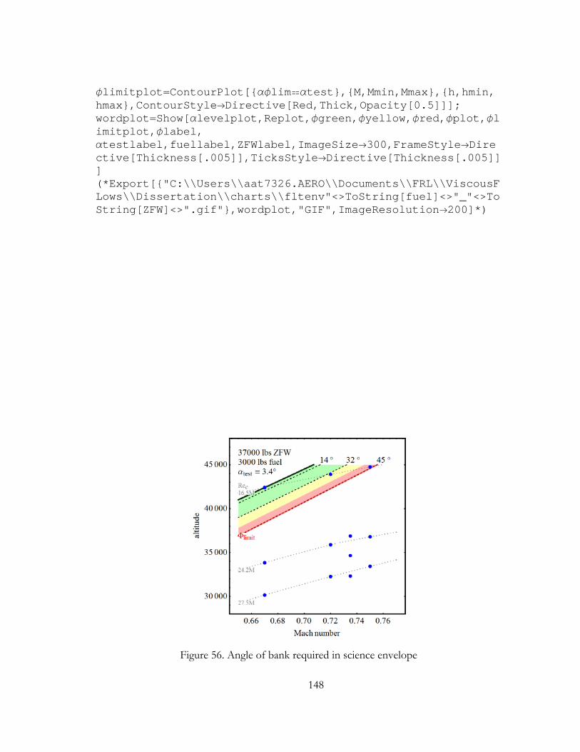
148

limitplot=ContourPlot[{limtest},{M,Mmin,Mmax},{h,hmin,hmax},ContourStyleDirective[Red,Thick,Opacity[0.5]]]; wordplot=Show[levelplot,Replot,green,yellow,red,plot,limitplot,label, testlabel,fuellabel,ZFWlabel,ImageSize300,FrameStyleDirective[Thickness[.005]],TicksStyleDirective[Thickness[.005]]] (*Export[{"C:\\Users\\aat7326.AERO\\Documents\\FRL\\ViscousFLows\\Dissertation\\charts\\fltenv"<>ToString[fuel]<>"_"<>ToString[ZFW]<>".gif"},wordplot,"GIF",ImageResolution200]*)

Figure 56. Angle of bank required in science envelope

149

A.7. Script for Figure 31. Angle of attack sensitivity to bank angle changes

da[_,_,h_,M_,fuel_]:=wt[fuel]/(q[h,M]S Cl)(Cos[]-Cos[+])/(Cos[]-Sin[+]Sin[]) (*angle to put the min/max fuel label*) Mtest=.735; (*current flight condition*) Retest=23.6*^6; testptno={9}; (*put the test point number on the chart*) Reh=h/.FindRoot[Rec[h,Mtest]Retest,{h,10000}]; plotmin=test-0.4; (*chart limits*) plotmax=test+0.4; plotmax=If[lim<45°,45°,lim+5°]; tol=0.1; (*calculate the fuel required for straight, level flight at flight condition to put in label*) fuellevel=fuel/.FindRoot[level[wt[fuel],Mtest,Reh]test,{fuel,4000}]; fuelint=1500; (*calculate the angle of bank for min fuel*) fuelmin=/.FindRoot[bank[,fuelmin,Mtest,Reh]plotmin,{,plotmax}]; fuelmin/Degree; fuelmin=bank[plotmax,fuelmin,Mtest,Reh]; fuelminlabel=Graphics[Rotate[Text[Style["min fuel",FontSizeMedium,BackgroundWhite],{If[fuelmin plotmax,plotmin,fuelmin],If[fuelminplotmax,fuelmin,plotmax]},{-1,-3}],Cos[2fuelmin]]]; fueltest=/.FindRoot[bank[,fuellevel,Mtest,Reh]test+tol,{,1°}]; fueltest=test+tol; fueltestlabel=Graphics[Rotate[Text[Style[ToString[fuellevel]<>" lbs fuel",FontSizeMedium,BackgroundWhite],{test+tol,If[fueltestplotmax,fueltest,plotmax]},{-1,-5}],Cos[7/2fueltest]]]; fuelmax=/.FindRoot[bank[,fuelmaxtest,Mtest,Reh]plotmax,{,1°}]; fuelmax=bank[fuelmax,fuelmaxtest,Mtest,Reh]; fuelmaxlabel=Graphics[Rotate[Text[Style["max fuel",FontSizeMedium,BackgroundWhite],{If[fuelmax plotmax,If[fuelmaxplotmax,fuelmax,plotmax],fuelmax],If[fuelmaxplotmax,fuelmax,plotmax]},{1,1}],Cos[1.5fuelmax]]];

150

fuellabel={fuelminlabel,fueltestlabel,fuelmaxlabel}; (*max bank angle label*) limitlabel=Graphics[Text[Style[Subscript["",limit],Red,FontSizeMedium,BackgroundWhite],{plotmin+.05,lim},{-1,0}]]; fuelplot=ParametricPlot[{{Table[{bank[,fuel,Mtest,Reh],},{fuel,fuellevel,fuellevel+8000,fuelint}]},{Table[{bank[,fuel,Mtest,Reh],},{fuel,fuellevel-fuelint,fuellevel-20000,-fuelint}]}},{,0°,plotmax},PlotStyle{Blue}]; testptlabel=Table[Graphics[Text[Style[i,Bold,White],{test,testptplan[[i,9]]},{0,0},BackgroundDirective[Brown,Opacity[0.8]]]],{i,testptno}]; (*calcualate fuel contours in two sets: less than level flight fuel to min fuel, greater than level flight fuel to max fuel*) back=ContourPlot[{},{,plotmin,plotmax},{,0,plotmax},Contours->{0,32°,40°,45°},ContourStyleNone,ContourShading{None,Directive[Green,Opacity[op]],Directive[Yellow,Opacity[op]],Directive[Red,Opacity[op]]},PlotRange{{plotmin,plotmax},{0°,plotmax}},FrameLabel{{"test",None},{"",ToString[Mtest]<>" M, "<>ToString[Retest/1*^6]<>"M Rec"}},FrameTicks{{{0°,10°,20°,32°,45°},{0°,10°,20°,32°,45°}},{{test-tol,test,test+tol},None}},FrameTrue,AxesFalse,LabelStyleDirective[Medium],ImageSize300,FrameStyleDirective[Thickness[.005]],TicksStyleDirective[Thickness[.005]],GridLines{None,{{lim,{Dashed,Red}}}},AspectRatio1]; fuelplotlim=ParametricPlot[{{bank[,fuelmaxtest,Mtest,Reh],},{bank[,fuelmin,Mtest,Reh],}},{,0°,plotmax},PlotStyle{Red,Thick,Dashed}]; lines={Graphics[{Dashed,Line[{{{test-tol,0},{test-tol,plotmax}},{{test+tol,0},{test+tol,plotmax}}}]}],Graphics[{Line[{{test,0},{test,plotmax}}]}]}; wordplot=Show[back,lines,fuelplot,fuelplotlim,fuellabel,limitlabel,testptlabel] (*Export[{"C:\\Users\\aat7326.AERO\\Documents\\FRL\\ViscousFLows\\Dissertation\\charts\\phi_alpha"<>ToString[Mtest]<>"_"<>ToString[Retest/1*^6]<>".gif"},wordplot,"GIF",ImageResolution200]*)

151

Figure 57. Angle of attack sensitivity to bank angle changes

152

A.8. Script for Figure 32. Deviation from test bank angle allowed within angle of

attack tolerance

ClearAll[fueltest,test,devp,delp]; dev=0.1; minm=14.5°; fueltest[test_]:=fuel/.FindRoot[bank[test,fuel,Mtest,Reh]test,{fuel,4000}] devaxis=Ceiling[(/.FindRoot[bank[,fueltest[0],Mtest,Reh]test+dev,{,0.1°}]),Pi/36]; devp[test_]:=/.FindRoot[bank[,fueltest[test],Mtest,Reh]test+dev,{,0.1°}] delp[test_]:=devp[test]-test devm[test_]:=/.FindRoot[bank[,fueltest[test],Mtest,Reh]test-dev,{,minm}] delm[test_]:=devm[test]-test limitlabel=Graphics[Rotate[Text[Style[Subscript["",limit],Red,FontSizeMedium,BackgroundWhite],{lim,devaxis},{-1,8}],-90°]]; delline=Graphics[{Line[{{0,0},{plotmax,0}}]}]; dellabel=Graphics[Text[Style["tol="<>ToString[dev]<>"°",Black,FontSizeMedium,BackgroundWhite],{lim,devaxis},{0,2}]]; back=ContourPlot[{test},{test,0,plotmax},{delp,-devaxis,devaxis},Contours->{0,32°,40°,45°},ContourStyleNone,ContourShading{None,Directive[Green,Opacity[op]],Directive[Yellow,Opacity[op]],Directive[Red,Opacity[op]]},PlotRange{{0°,plotmax},{-devaxis,devaxis}},FrameLabel{{"",None},{"test",None(*ToString[Mtest]<>" M, "<>ToString[Retest/1*^6]<>"M Subscript[Re, c], Subscript[, tol]="<>ToString[dev]<>"°"}*)}},FrameTicks{{{-15°,-10°,-5°,0°,5°,10°,15°},None},{{0°,10°,20°,32°,45°},None}},GridLines{{{lim,{Dashed,Red}}},None},FrameTrue,ImageSize450,LabelStyleDirective[Medium],FrameStyleDirective[Thickness[.005]],TicksStyleDirective[Thickness[.005]]]; plotp=ParametricPlot[{test,delp[test]},{test,0°,plotmax},PlotStyle{Thick,Blue}]; (*plot test points on the chart*) testptplotdel=ListPlot[Table[{testptplan[[i,9]],0},{i,numtestpts}],PlotStyleBrown,PlotMarkers{Automatic,Medium}];

153

plotm=ParametricPlot[{test,delm[test]},{test,minm,plotmax},PlotStyle{Thick,Blue}]; wordplot=Show[back,plotp,plotm,limitlabel,delline,testptplotdel,dellabel,ImageSize400,AspectRatio1/GoldenRatio] (*Export[{"C:\\Users\\aat7326.AERO\\Documents\\FRL\\ViscousFLows\\Dissertation\\charts\\phi_deltaphi"<>"_"<>ToString[dev]<>".gif"},wordplot,"GIF",ImageResolution200]*)

Figure 58. Deviation from test bank angle allowed within angle of attack tolerance

154

A.9. Script for Figure 37. Angle of attack perturbation detection

Needs["HypothesisTesting`"] Needs["ErrorBarPlots`"] data=Import["C:\\Users\\aat7326.AERO\\Documents\\FRL\\ViscousFLows\\Dissertation\\analysis\\Dive data\\dive data.csv"]; Transpose[data]; data[[1,-1]]=StringJoin[Characters[data[[1,-2]]][[;;6]]]<>" + 0.5°"; data[[2;;21,-1]]=data[[2;;21,-2]]+0.5; data[[2;;21,;;-1]]//Grid a0=data[[2;;21]]; a=data[[2;;21,;;-2]]; s=Dimensions[a][[1]]; n=Dimensions[a][[2]]; barn=Mean[a0]; varn=Variance[a0]; n=StandardDeviation[a0]; Transpose[{barn,n}]; bar=Mean[Flatten[a]]; var=Variance[Flatten[a]]; =StandardDeviation[Flatten[a]]; ci=StudentTCI[bar,,n s-1]; mse=Sum[varn[[j]],{j,n}]/n; tstat[_,_]:=t/.FindRoot[CDF[StudentTDistribution[],t](1-),{t,0.2}]; tstat[0.025,n(s-1)]; lsd=tstat[0.025,n(s-1)] Sqrt[2 mse/s]; Print["LSD = ",lsd] ciline=Table[{i,j},{j,ci},{i,{0,Dimensions[a][[2]]}}]; dateticks=Table[{n,Text[Rotate[data[[1,n]],80°,{0,1}]]},{n,Dimensions[data][[2]]}]; errplot=ErrorListPlot[Transpose[{barn,n}],PlotRange{-0.6,0.8},FrameTicks{{Range[-0.8,0.8,0.2],None},{dateticks,None}},FrameTrue,PlotStyle{Black,Thin},PlotLabel"O-2A 4000 ft, Rec=7.5M",AxesNone,FrameLabel{None,"angle of attack [°]"}]; barplot=ListLinePlot[{{0,bar},{Dimensions[a][[2]],bar}},PlotStyle{Blue,Thick,Opacity[0.9]}]; plot=ListLinePlot[{{{0,bar+},{Dimensions[a][[2]],bar+}},{{0,bar-},{Dimensions[a][[2]],bar-}}},PlotStyleDirective[Blue,Thin,Dashed,Opacity[0.9]]];

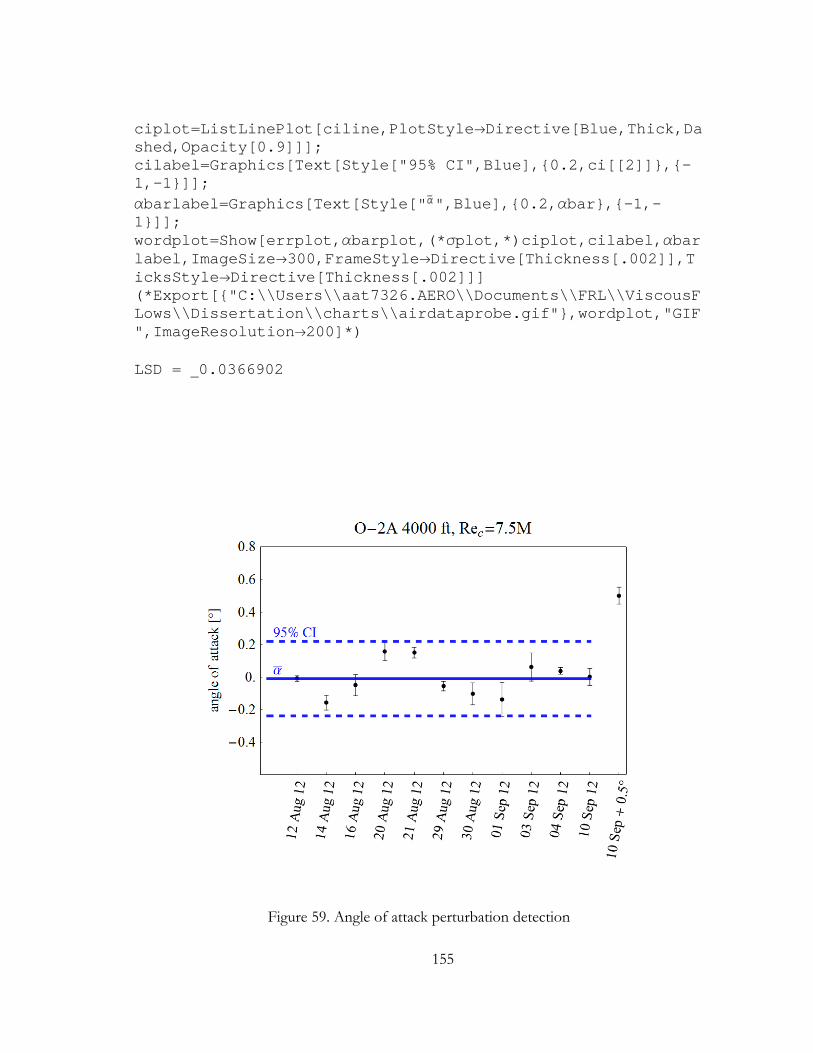
155

ciplot=ListLinePlot[ciline,PlotStyleDirective[Blue,Thick,Dashed,Opacity[0.9]]]; cilabel=Graphics[Text[Style["95% CI",Blue],{0.2,ci[[2]]},{-1,-1}]]; barlabel=Graphics[Text[Style[" ",Blue],{0.2,bar},{-1,-1}]]; wordplot=Show[errplot,barplot,(*plot,*)ciplot,cilabel,barlabel,ImageSize300,FrameStyleDirective[Thickness[.002]],TicksStyleDirective[Thickness[.002]]] (*Export[{"C:\\Users\\aat7326.AERO\\Documents\\FRL\\ViscousFLows\\Dissertation\\charts\\airdataprobe.gif"},wordplot,"GIF",ImageResolution200]*) LSD = _0.0366902

Figure 59. Angle of attack perturbation detection