Embed Size (px)
Citation preview
Computer Animation
AYBU - CENG505 Advanced Computer Graphics
Computer Animation = Making Things Move
Computer Animation Used In
n Movies n Special Effects n Games n Human Computer Interaction n Scientific / Data Visualization
Topic Overview
n Traditional animation process n Keyframing and interpolation n Modeling and animating articulated figures n Motion capture n Motion editing n Physically based (dynamics) n Natural phenomena (plants, water, gas) n Rendering issues (compositing, motion blur…) n Other research topics
Traditional Animation
n Computer animation builds on techniques and tools from traditional animation.
n Film runs at 24 frames per second (fps) q That’s 1440 pictures to create per minute q 1800 fpm for video (30 fps)
n ~200.000 frames for a 90 min movie
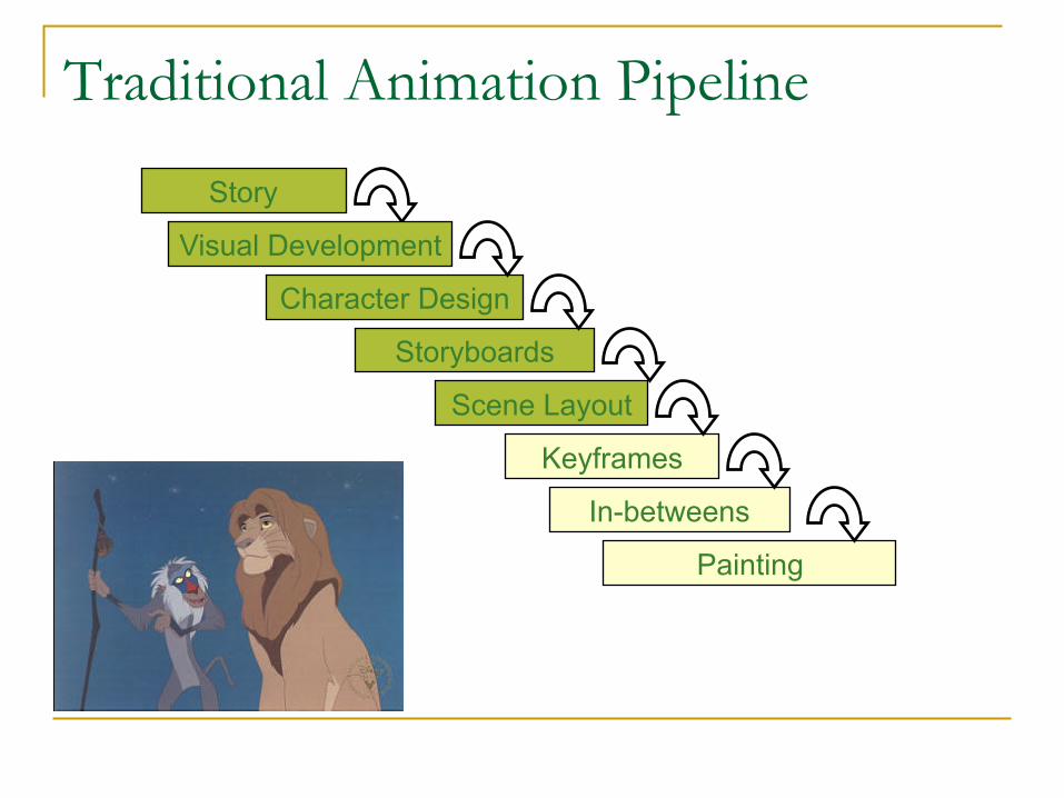
Traditional Animation Pipeline
Story
Storyboards Scene Layout
Character Design
Visual Development
Keyframes In-betweens
Painting
Traditional Animation: The Process
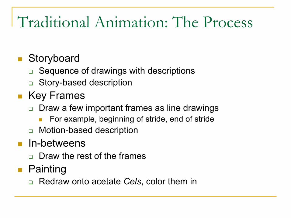
n Storyboard q Sequence of drawings with descriptions q Story-based description
n Key Frames q Draw a few important frames as line drawings
n For example, beginning of stride, end of stride q Motion-based description
n In-betweens q Draw the rest of the frames
n Painting q Redraw onto acetate Cels, color them in
Traditional Animation: Storyboarding
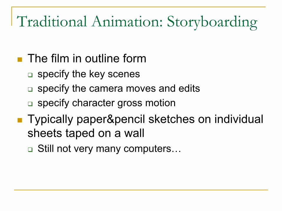
n The film in outline form q specify the key scenes q specify the camera moves and edits q specify character gross motion
n Typically paper&pencil sketches on individual sheets taped on a wall q Still not very many computers…
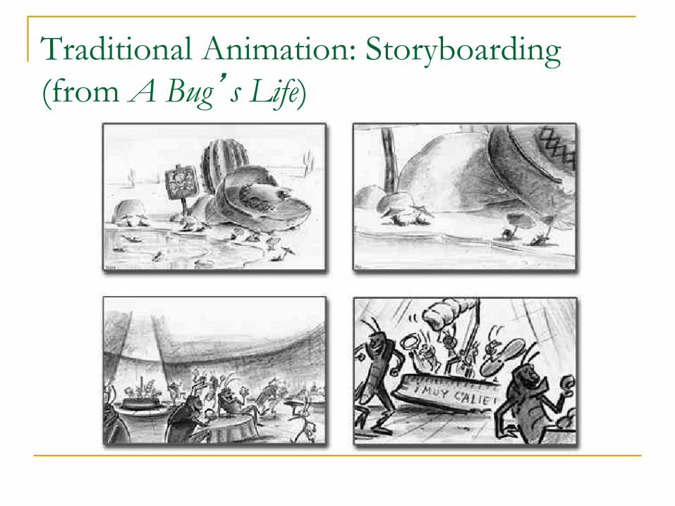
Traditional Animation: Storyboarding (from A Bug’s Life)
Storyboarding: Key Issues
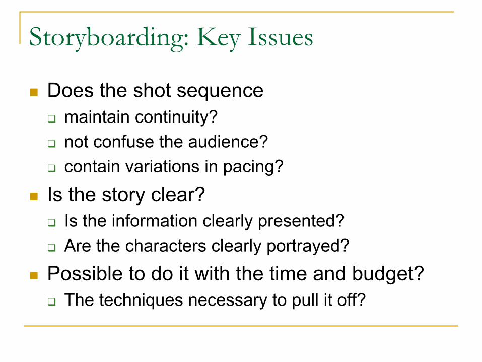
n Does the shot sequence q maintain continuity? q not confuse the audience? q contain variations in pacing?
n Is the story clear? q Is the information clearly presented? q Are the characters clearly portrayed?
n Possible to do it with the time and budget? q The techniques necessary to pull it off?
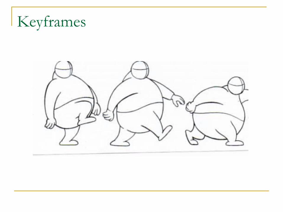
Keyframes
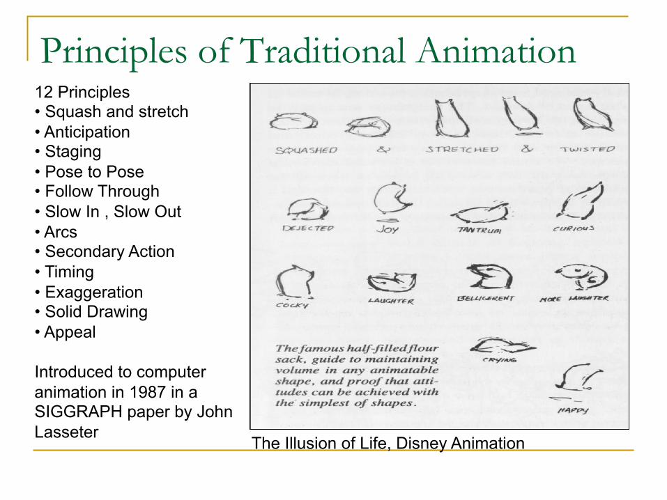
Principles of Traditional Animation 12 Principles • Squash and stretch • Anticipation • Staging • Pose to Pose • Follow Through • Slow In , Slow Out • Arcs • Secondary Action • Timing • Exaggeration • Solid Drawing • Appeal Introduced to computer animation in 1987 in a SIGGRAPH paper by John Lasseter The Illusion of Life, Disney Animation
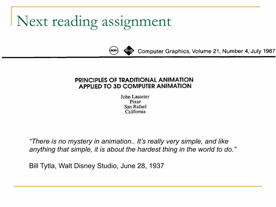
Next reading assignment
“There is no mystery in animation.. It’s really very simple, and like anything that simple, it is about the hardest thing in the world to do.”
Bill Tytla, Walt Disney Studio, June 28, 1937
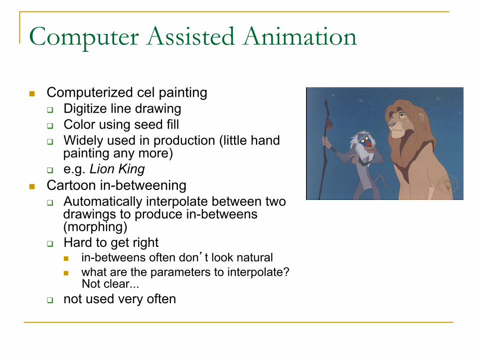
Computer Assisted Animation
n Computerized cel painting q Digitize line drawing q Color using seed fill q Widely used in production (little hand
painting any more) q e.g. Lion King
n Cartoon in-betweening q Automatically interpolate between two
drawings to produce in-betweens (morphing)
q Hard to get right n in-betweens often don’t look natural n what are the parameters to interpolate?
Not clear... q not used very often
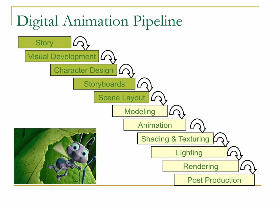
Digital Animation Pipeline Story
Storyboards Scene Layout
Character Design
Visual Development
Modeling Animation Shading & Texturing
Lighting Rendering
Post Production
Principles of Traditional Animation
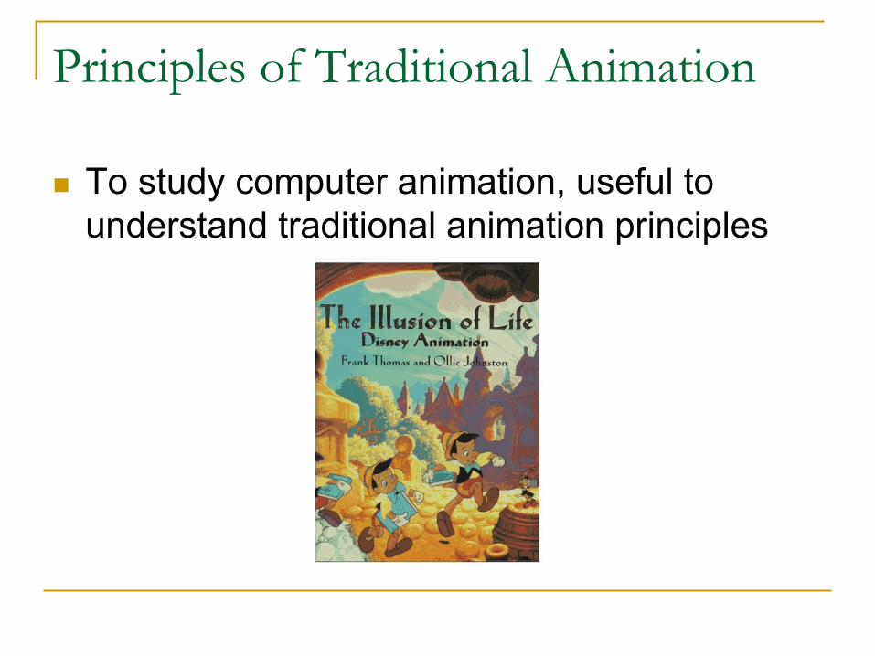
Principles of Traditional Animation
n To study computer animation, useful to understand traditional animation principles
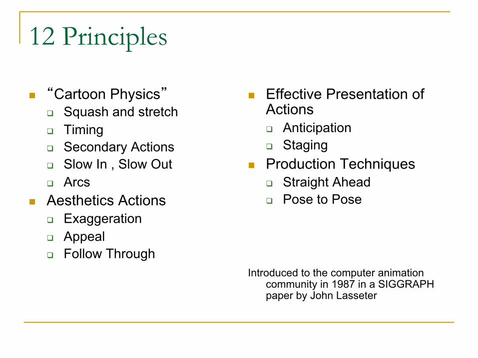
12 Principles
n “Cartoon Physics” q Squash and stretch q Timing q Secondary Actions q Slow In , Slow Out q Arcs
n Aesthetics Actions q Exaggeration q Appeal q Follow Through
n Effective Presentation of Actions q Anticipation q Staging
n Production Techniques q Straight Ahead q Pose to Pose
Introduced to the computer animation community in 1987 in a SIGGRAPH paper by John Lasseter

Video
n Luxo Jr. (again)
n Geri’s Game

12 Principles
n “Cartoon Physics” q Squash and stretch q Timing q Secondary Actions q Slow In , Slow Out q Arcs
n Aesthetics Actions q Exaggeration q Appeal q Follow Through
n Effective Presentation of Actions q Anticipation q Staging
n Production Techniques q Straight Ahead q Pose to Pose
Introduced to the computer animation community in 1987 in a SIGGRAPH paper by John Lasseter
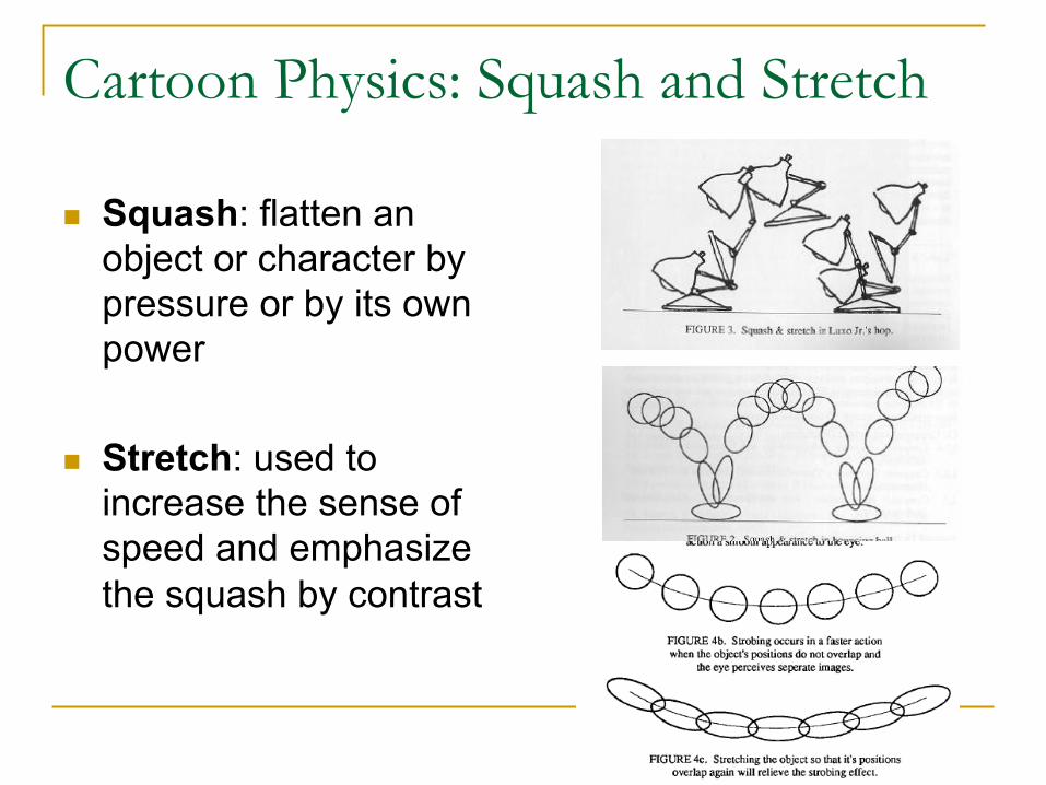
Cartoon Physics: Squash and Stretch
n Squash: flatten an object or character by pressure or by its own power
n Stretch: used to increase the sense of speed and emphasize the squash by contrast
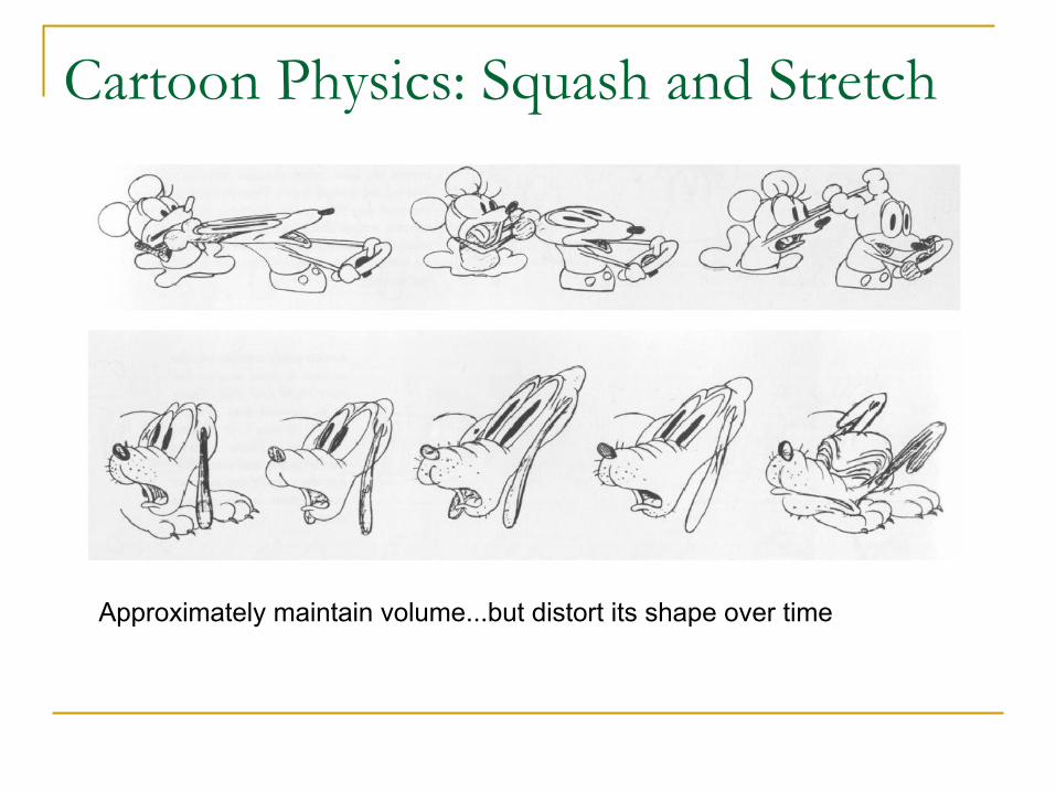
Cartoon Physics: Squash and Stretch
Approximately maintain volume...but distort its shape over time
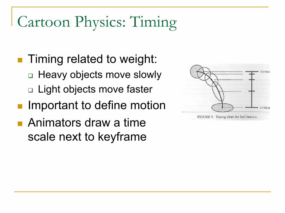
Cartoon Physics: Timing
n Timing related to weight: q Heavy objects move slowly q Light objects move faster
n Important to define motion n Animators draw a time
scale next to keyframe

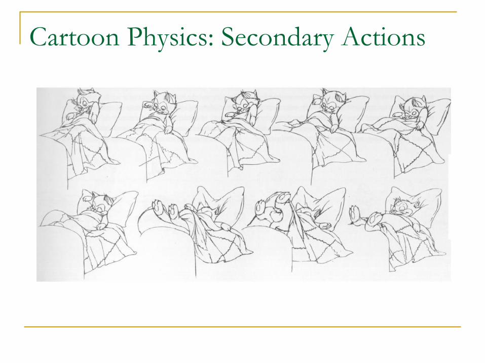
Cartoon Physics: Secondary Actions
n A secondary action is an action that results directly from another action
n Usually, secondary actions support main action and typically represent physical reactions
n Important in heightening interest and adding a realistic complexity to the animation
Cartoon Physics: Secondary Actions
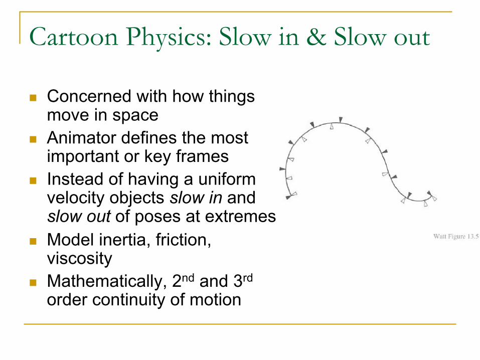
Cartoon Physics: Slow in & Slow out
n Concerned with how things move in space
n Animator defines the most important or key frames
n Instead of having a uniform velocity objects slow in and slow out of poses at extremes
n Model inertia, friction, viscosity
n Mathematically, 2nd and 3rd order continuity of motion
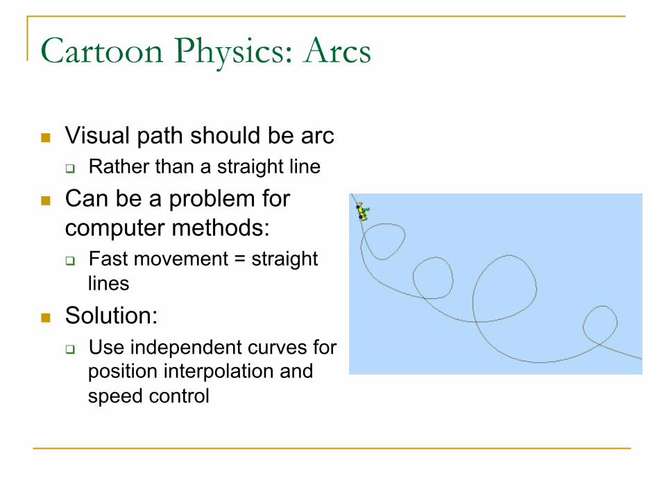
Cartoon Physics: Arcs
n Visual path should be arc q Rather than a straight line
n Can be a problem for computer methods: q Fast movement = straight
lines n Solution:
q Use independent curves for position interpolation and speed control
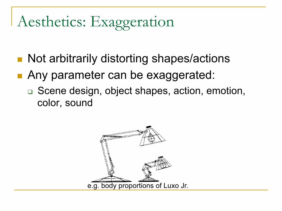
Aesthetics: Exaggeration
n Not arbitrarily distorting shapes/actions n Any parameter can be exaggerated:
q Scene design, object shapes, action, emotion, color, sound
e.g. body proportions of Luxo Jr.
Aesthetics: Appeal
n Creating a design or an action that the audience enjoys watching
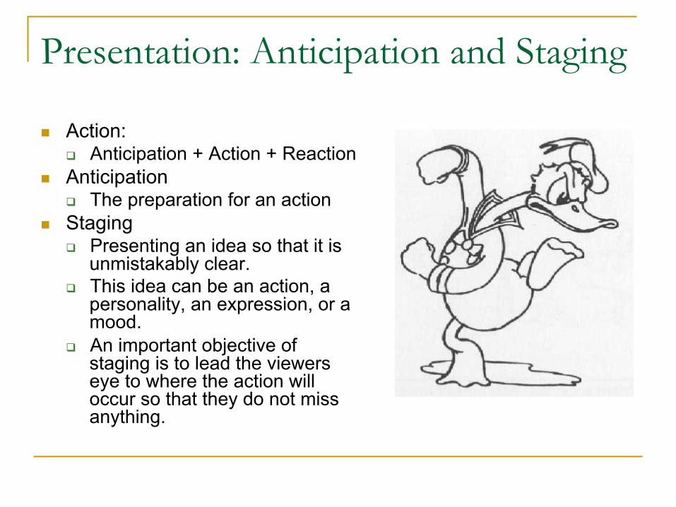
Presentation: Anticipation and Staging
n Action: q Anticipation + Action + Reaction
n Anticipation q The preparation for an action
n Staging q Presenting an idea so that it is
unmistakably clear. q This idea can be an action, a
personality, an expression, or a mood.
q An important objective of staging is to lead the viewers eye to where the action will occur so that they do not miss anything.
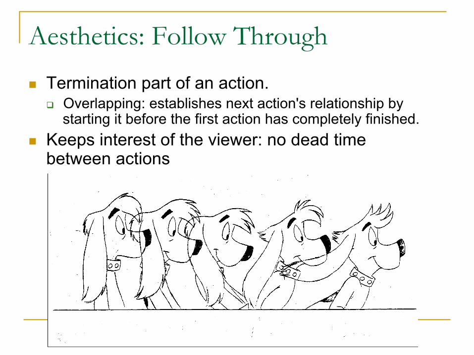
Aesthetics: Follow Through
n Termination part of an action. q Overlapping: establishes next action's relationship by
starting it before the first action has completely finished. n Keeps interest of the viewer: no dead time
between actions
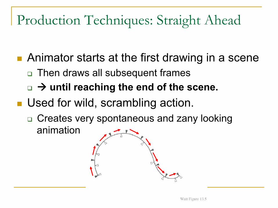
Production Techniques: Straight Ahead
n Animator starts at the first drawing in a scene q Then draws all subsequent frames q à until reaching the end of the scene.
n Used for wild, scrambling action. q Creates very spontaneous and zany looking
animation
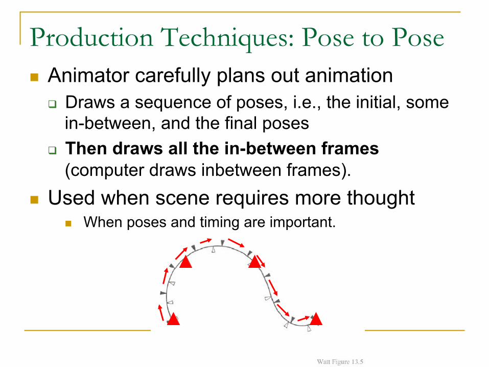
Production Techniques: Pose to Pose n Animator carefully plans out animation
q Draws a sequence of poses, i.e., the initial, some in-between, and the final poses
q Then draws all the in-between frames (computer draws inbetween frames).
n Used when scene requires more thought n When poses and timing are important.
Traditional to computerized
n Traditional animation uses 12 design principles to create ‘illusion of life’
n Computer animation borrows these techniques from traditional animation
n Further information: q Thomas, Johnson, The Illusion of Life: Disney Animation (~1000
pages, suggested if you want to know traditional animation principles)
Keyframing
What is a Key?
n Anything can be keyframed and interpolated q Position, Orientation, Scale, Deformation, Patch
Control Points (facial animation), Color, Surface Normals…
n Special interpolation schemes for some types of parameters (e.g. rotations) q Use quaternions to represent rotation and
interpolate between quaternions n Control of parameterization controls speed of
animation
Keyframing Basics
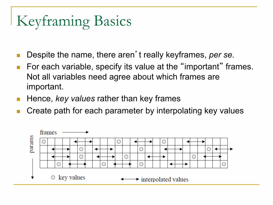
n Despite the name, there aren’t really keyframes, per se. n For each variable, specify its value at the “important” frames.
Not all variables need agree about which frames are important.
n Hence, key values rather than key frames n Create path for each parameter by interpolating key values
Keyframing Recipe
n Specify the key frames q rigid transforms, forward kinematics, inverse
kinematics n Specify the type of interpolation
q linear, cubic, parametric curves n Specify the speed profile of the interpolation
q constant velocity, ease-in,out, etc. n Computer generates the in-between frames
Keyframing Pros and Cons
n Gives good control over motion n Eliminates much of the labor of traditional animation
q But still very labor-intensive
n Impractical for complex scenes with everything moving: q grass in the wind, water, and crowd scenes, for example
n Now, in more detail: q how to interpolate and what to interpolate (positions for this
lecture, orientations next time)
Keyframing
n Interpolation n Motion Along a Curve (arc length) n Interpolation of Rotations (quaternions) n Path following
Interpolation
n Foundation of animation is interpolation of values. n Given: a list of values associated with a given
parameter at specific frames (called key frames or keys) of the animation.
n Goal: how best to generate the values of the parameter for the frames between the key frames.
n The parameter to be interpolated may be q a coordinate of the position of an object, q a joint angle of an appendage of a robot, q the transparency attribute of an object, q any other parameter
Interpolation
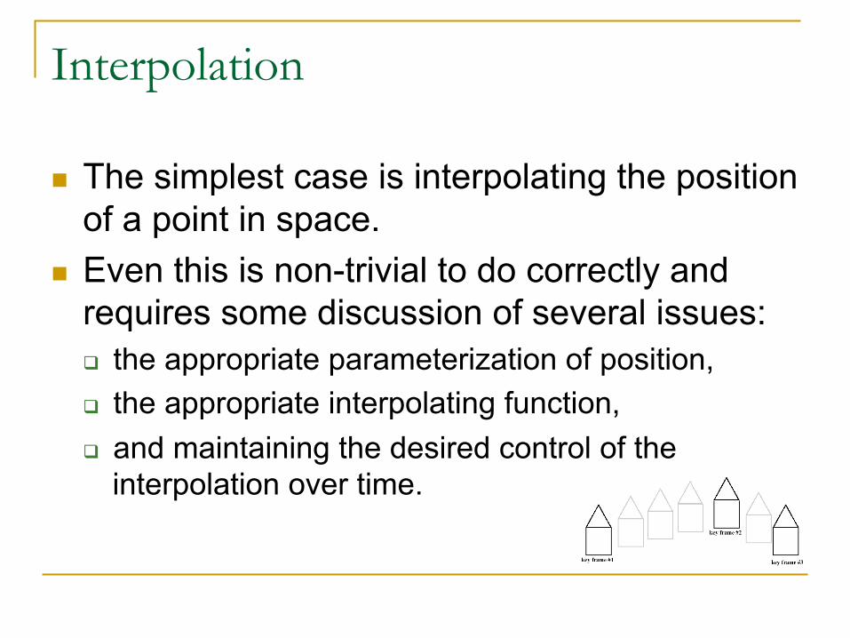
n The simplest case is interpolating the position of a point in space.
n Even this is non-trivial to do correctly and requires some discussion of several issues: q the appropriate parameterization of position, q the appropriate interpolating function, q and maintaining the desired control of the
interpolation over time.
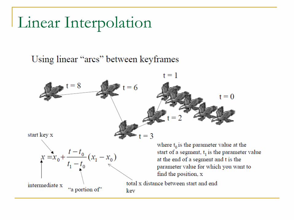
Linear Interpolation
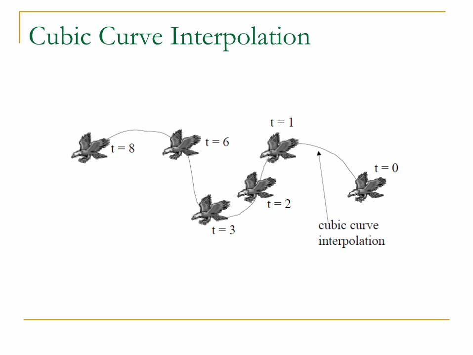
Cubic Curve Interpolation
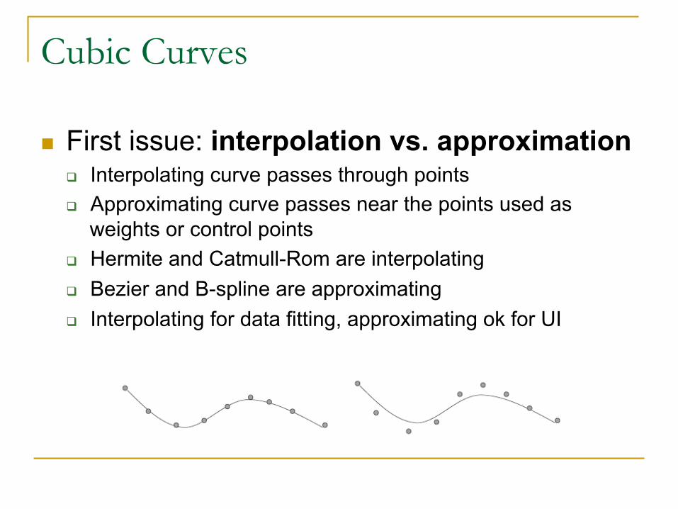
Cubic Curves
n First issue: interpolation vs. approximation q Interpolating curve passes through points q Approximating curve passes near the points used as
weights or control points q Hermite and Catmull-Rom are interpolating q Bezier and B-spline are approximating q Interpolating for data fitting, approximating ok for UI
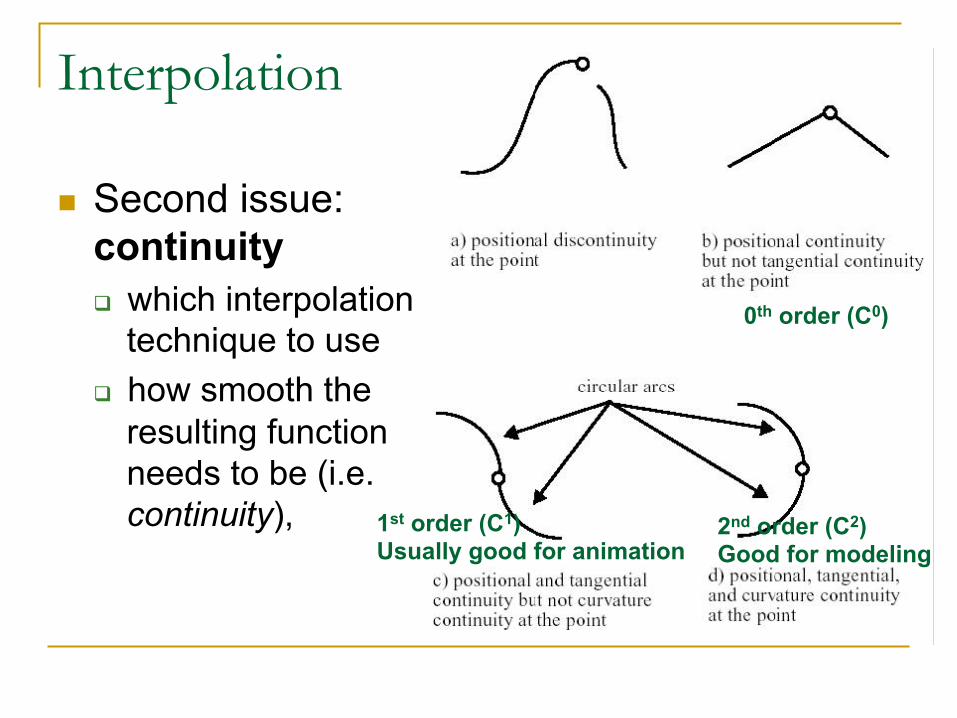
Interpolation
n Second issue: continuity q which interpolation
technique to use q how smooth the
resulting function needs to be (i.e. continuity), 1st order (C1)
Usually good for animation 2nd order (C2) Good for modeling
0th order (C0)
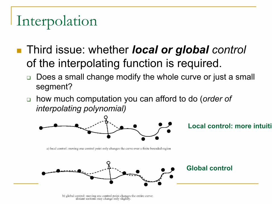
Interpolation
n Third issue: whether local or global control of the interpolating function is required. q Does a small change modify the whole curve or just a small
segment? q how much computation you can afford to do (order of
interpolating polynomial)
Local control: more intuitive
Global control
Interpolation
n Local control is more intuitive: q Almost all composite curves provide local control
n Curves which provide local control: q Parabolic blending q Catmull-Rom splines q Composite cubic Bezier q Cubic B-spline
n Other curves provide less local control q Hermite curves q Higher-order Bezier and B-Spline curves
Interpolation
n Curves play major role in interpolation
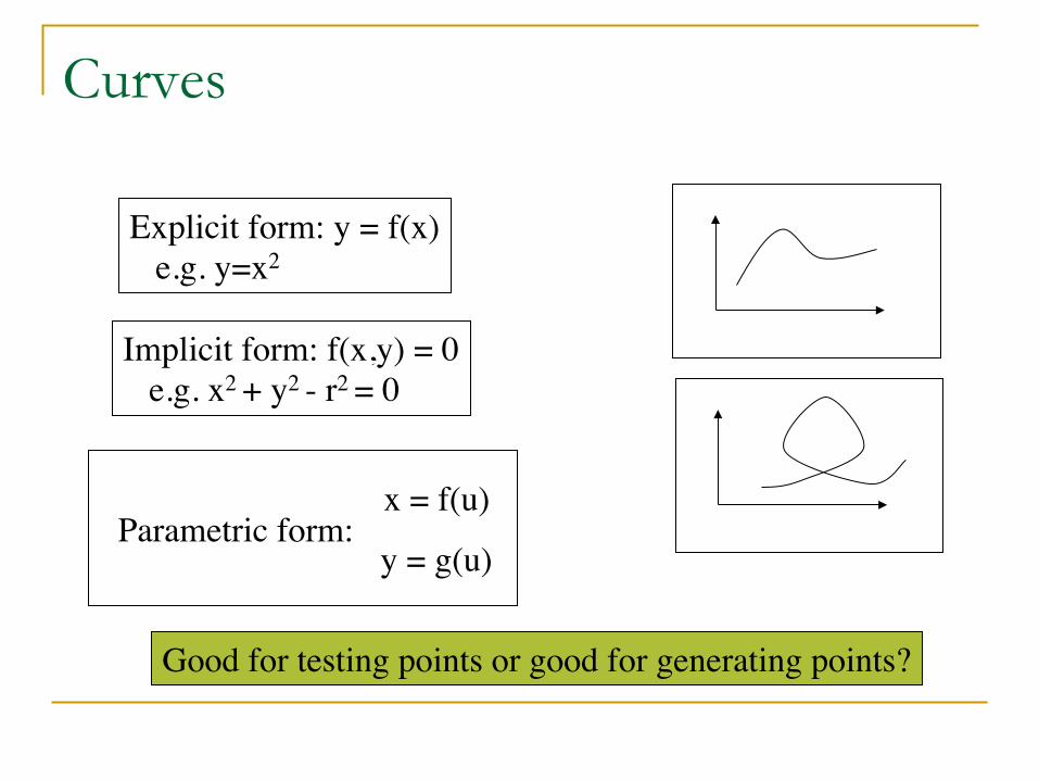
Curves
Explicit form: y = f(x) e.g. y=x2
Implicit form: f(x,y) = 0 e.g. x2 + y2 - r2 = 0
x = f(u)
y = g(u)Parametric form:
Good for testing points or good for generating points?
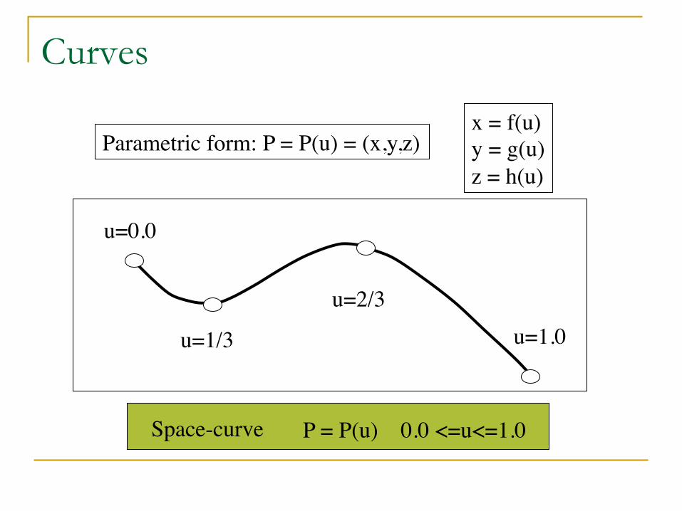
Curves
Space-curve P = P(u) 0.0 <=u<=1.0
u=1/3
u=2/3
u=0.0
u=1.0
Parametric form: P = P(u) = (x,y,z)x = f(u)y = g(u)z = h(u)
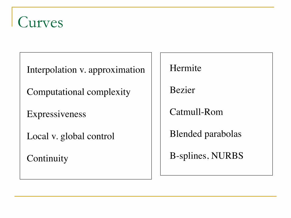
Curves
Local v. global control
Computational complexity
Continuity
Interpolation v. approximation Hermite
Bezier
Catmull-Rom
Blended parabolas
Expressiveness
B-splines, NURBS
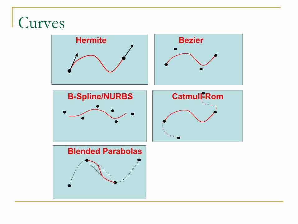
Curves Hermite Bezier
B-Spline/NURBS Catmull-Rom
Blended Parabolas
Summary
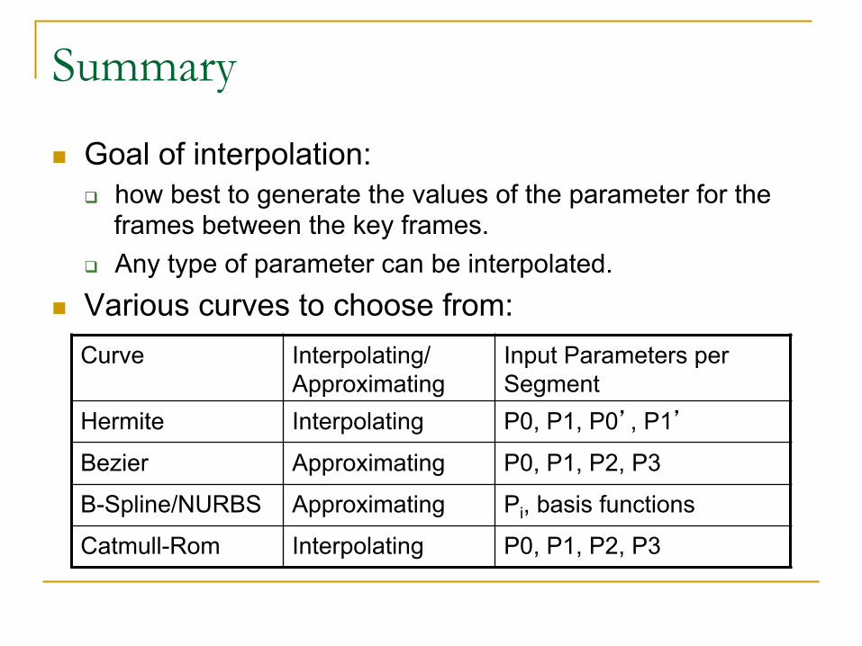
n Goal of interpolation: q how best to generate the values of the parameter for the
frames between the key frames. q Any type of parameter can be interpolated.
n Various curves to choose from: Curve Interpolating/
Approximating Input Parameters per Segment
Hermite Interpolating P0, P1, P0’, P1’
Bezier Approximating P0, P1, P2, P3
B-Spline/NURBS Approximating Pi, basis functions
Catmull-Rom Interpolating P0, P1, P2, P3
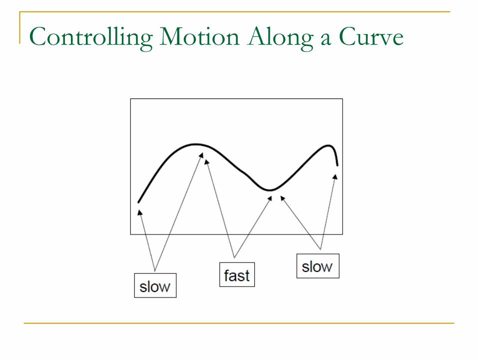
Controlling Motion Along a Curve
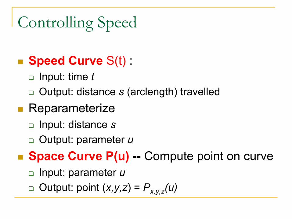
Controlling Speed
n Speed Curve S(t) : q Input: time t q Output: distance s (arclength) travelled
n Reparameterize q Input: distance s q Output: parameter u
n Space Curve P(u) -- Compute point on curve q Input: parameter u q Output: point (x,y,z) = Px,y,z(u)
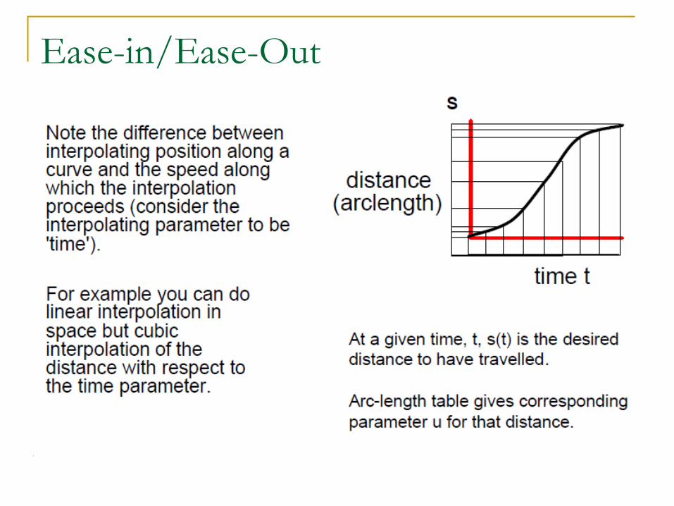
Ease-in/Ease-Out
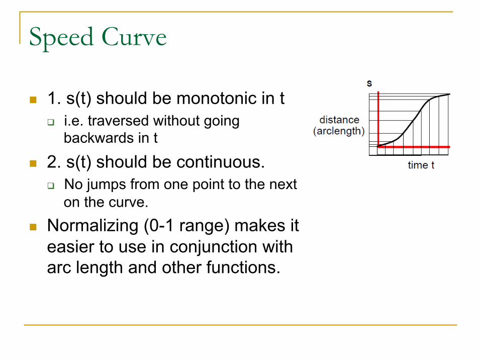
Speed Curve
n 1. s(t) should be monotonic in t q i.e. traversed without going
backwards in t
n 2. s(t) should be continuous. q No jumps from one point to the next
on the curve. n Normalizing (0-1 range) makes it
easier to use in conjunction with arc length and other functions.
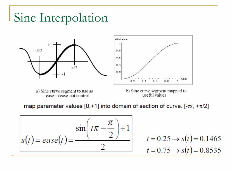
Sine Interpolation
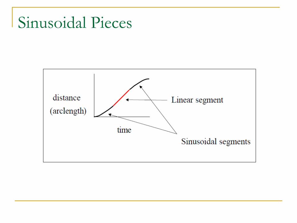
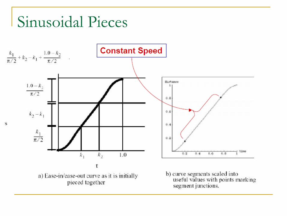
Sinusoidal Pieces n Another method is to have user specify times t1, t2. n A sinusoidal curve is used for velocity to implement
an acceleration from time 0 to t1. n A sinusoidal curve is also used for velocity to
implement deceleration from time t2 to 1. n Between times t1 and t2, constant velocity is used. n Done by taking parameter t in the range 0 to 1:
q and remapping it into that range according to the above velocity curves to get a new parameter rt.
n So as t varies uniformly from 0 to 1, rt will accelerate from 0, then maintain a constant parametric velocity and then decelerate back to 1.
Sinusoidal Pieces
Sinusoidal Pieces
Parabolic Ease-In/Ease-Out
n Instead of sinusoidal, use parabolic ease in/out n An alternative approach and one that avoids:
q the transcendental function evaluation (sin, cos) q or corresponding table look-up and interpolation
n …is to establish basic assumptions about the acceleration and, from there, integrate to get the resulting interpolation function.
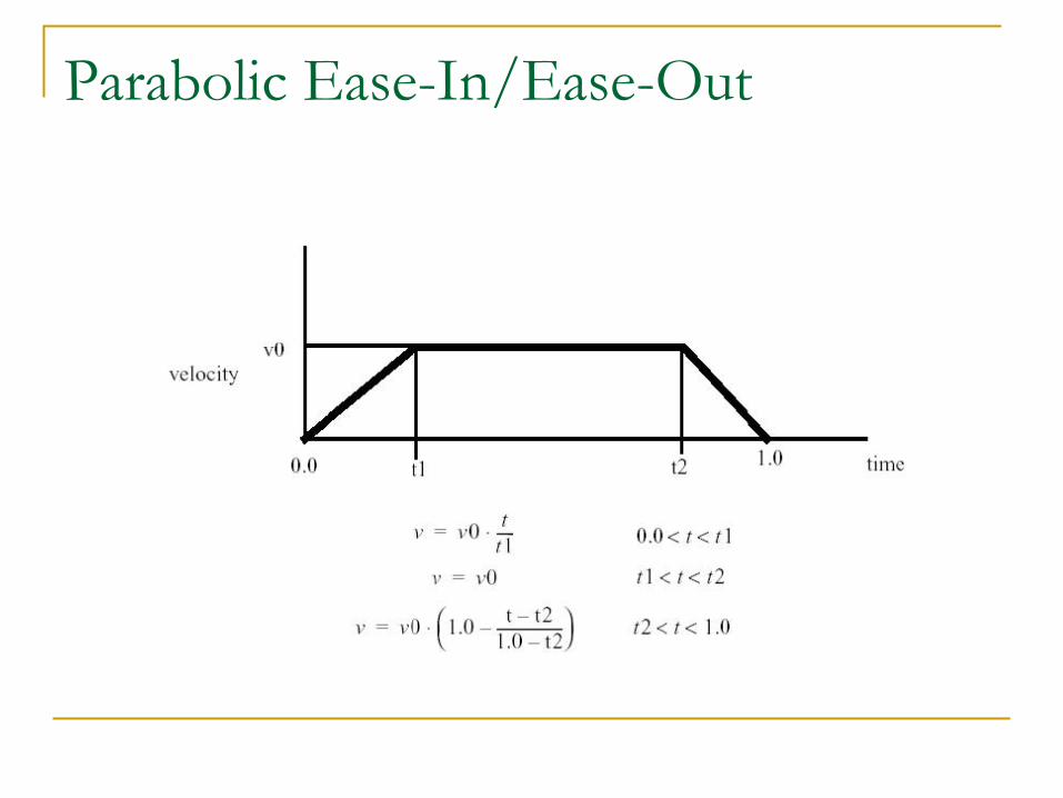
Parabolic Ease-In/Ease-Out
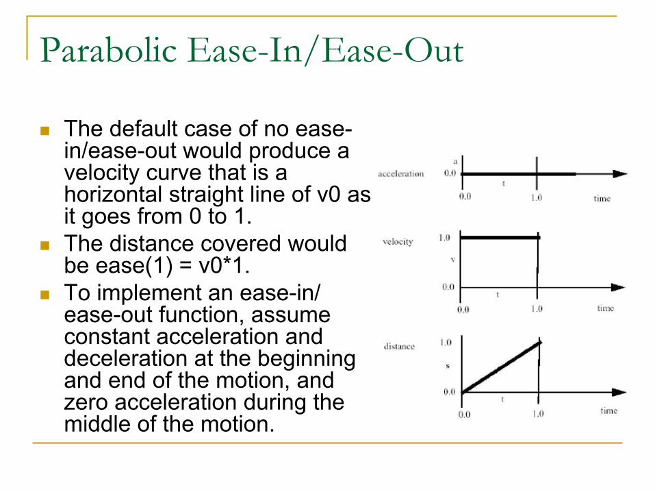
n The default case of no ease-in/ease-out would produce a velocity curve that is a horizontal straight line of v0 as it goes from 0 to 1.
n The distance covered would be ease(1) = v0*1.
n To implement an ease-in/ease-out function, assume constant acceleration and deceleration at the beginning and end of the motion, and zero acceleration during the middle of the motion.
Parabolic Ease-In/Ease-Out
Parabolic Ease-In/Ease-Out
Parabolic Ease-In/Ease-Out
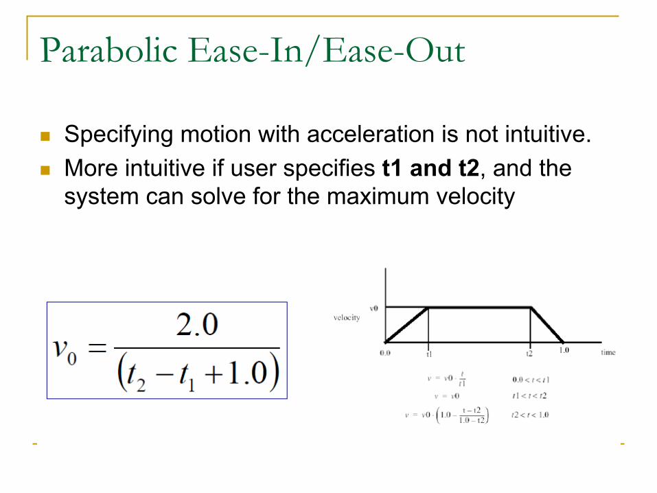
n Specifying motion with acceleration is not intuitive. n More intuitive if user specifies t1 and t2, and the
system can solve for the maximum velocity
Parabolic Ease-In/Ease-Out
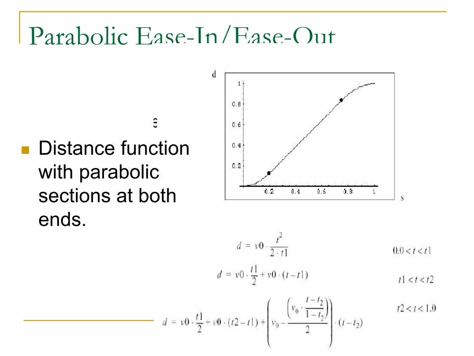
n Distance function with parabolic sections at both ends.
Parabolic Ease-In/Ease-Out
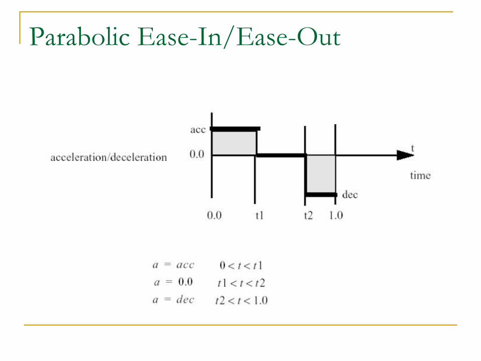
n Distance in this case is in parametric space, or t-space, and is the distance covered by the output value of t.
n For a given range of t = [0,1], the user specifies times to control acceleration and deceleration: t1 and t2.
n Acceleration occurs from time 0 to time t1. n Deceleration occurs from time t2 to time 1.
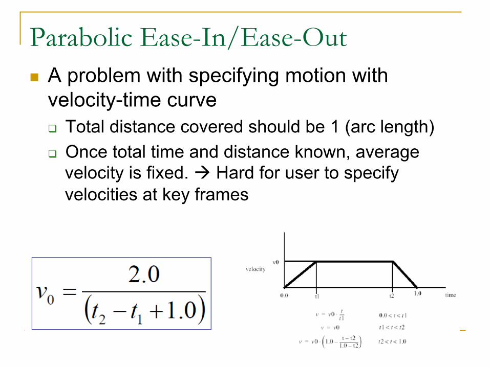
Parabolic Ease-In/Ease-Out n A problem with specifying motion with
velocity-time curve q Total distance covered should be 1 (arc length) q Once total time and distance known, average
velocity is fixed. à Hard for user to specify velocities at key frames
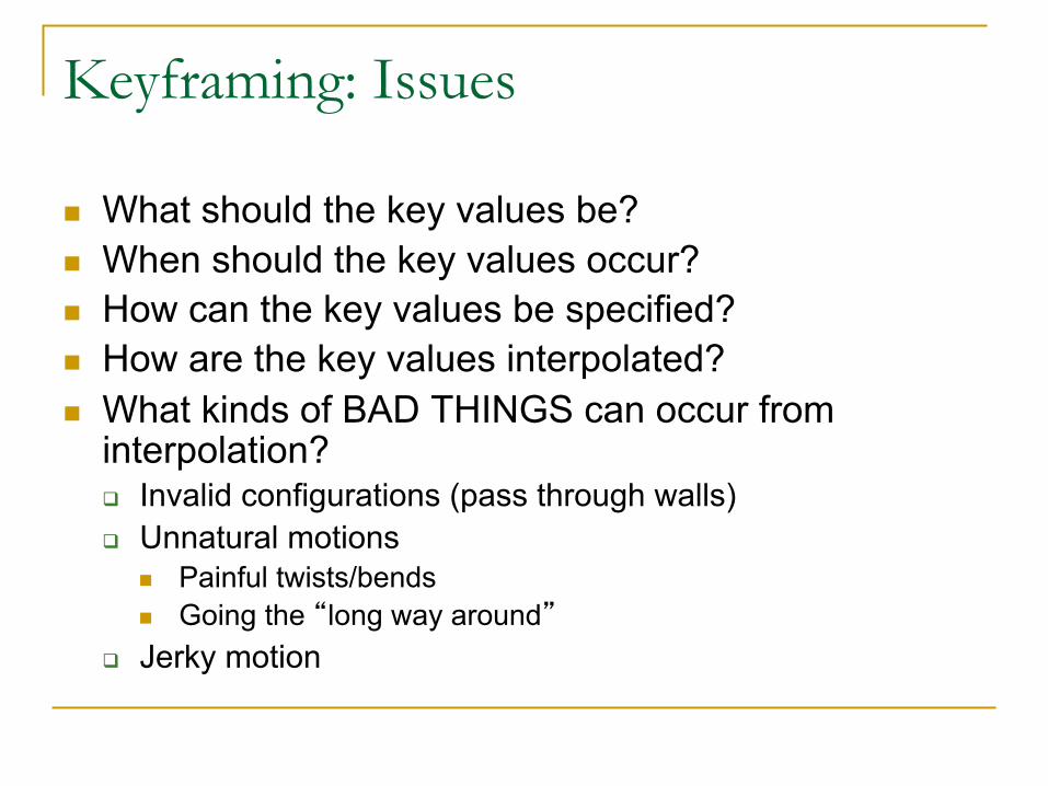
Keyframing: Issues
n What should the key values be? n When should the key values occur? n How can the key values be specified? n How are the key values interpolated? n What kinds of BAD THINGS can occur from
interpolation? q Invalid configurations (pass through walls) q Unnatural motions
n Painful twists/bends n Going the “long way around”
q Jerky motion
Deformation
Object Deformation
n Many objects are not rigid q jello q mud q gases/liquids q etc.
n Two main techniques: q Geometric deformations – this lecture
n Deforms object mesh / geometry directly q Physically-based methods – later in course
n Physically accurate simulation of objects n What is main difference between these two in terms
of creation?
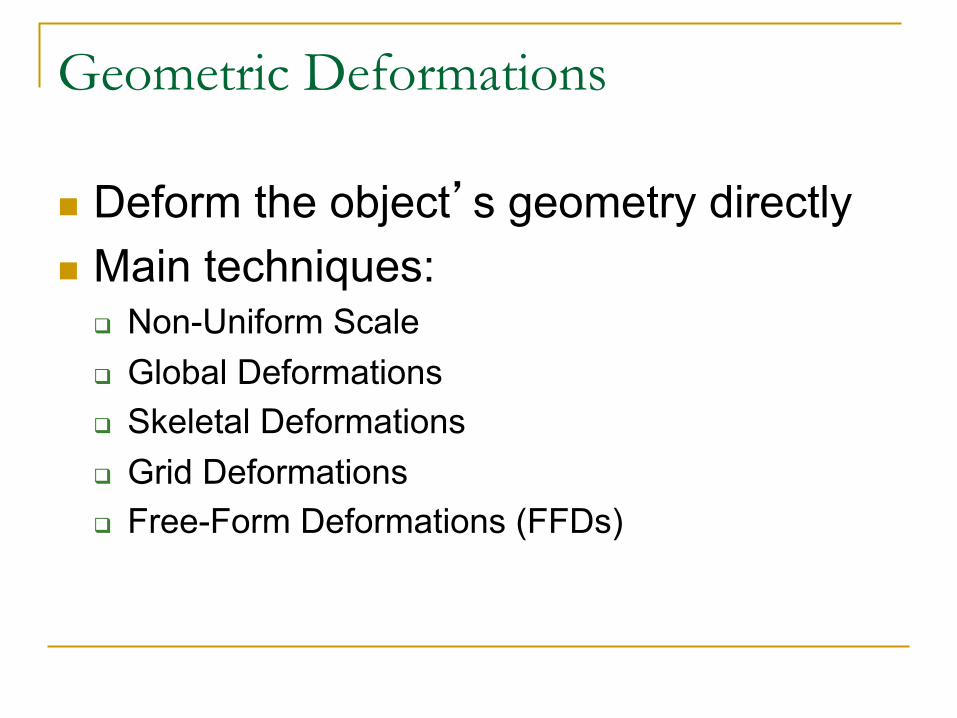
Geometric Deformations
n Deform the object’s geometry directly n Main techniques:
q Non-Uniform Scale q Global Deformations q Skeletal Deformations q Grid Deformations q Free-Form Deformations (FFDs)
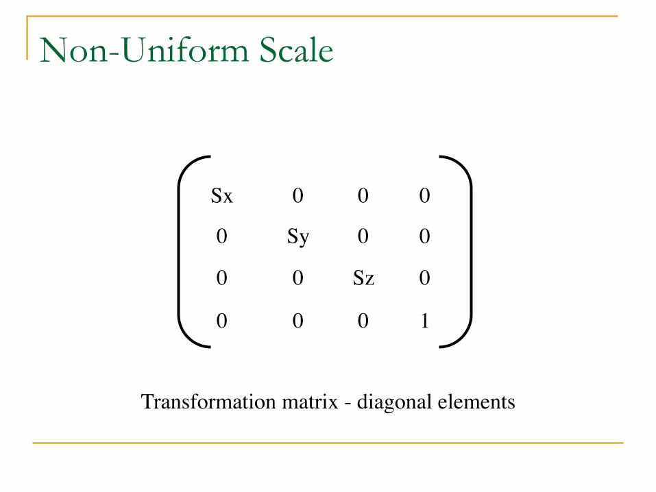
Transformation matrix - diagonal elements
0
1
Sx
Sy
Sz
0
0
0
0
0
0 0
0
00 0
Non-Uniform Scale
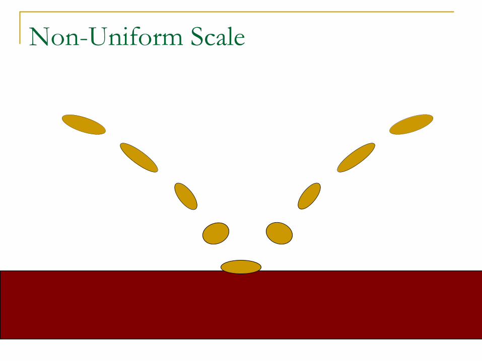
Non-Uniform Scale
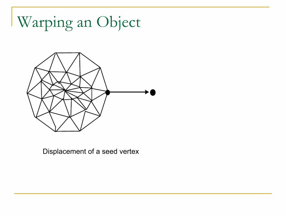
Warping an Object
Displacement of a seed vertex
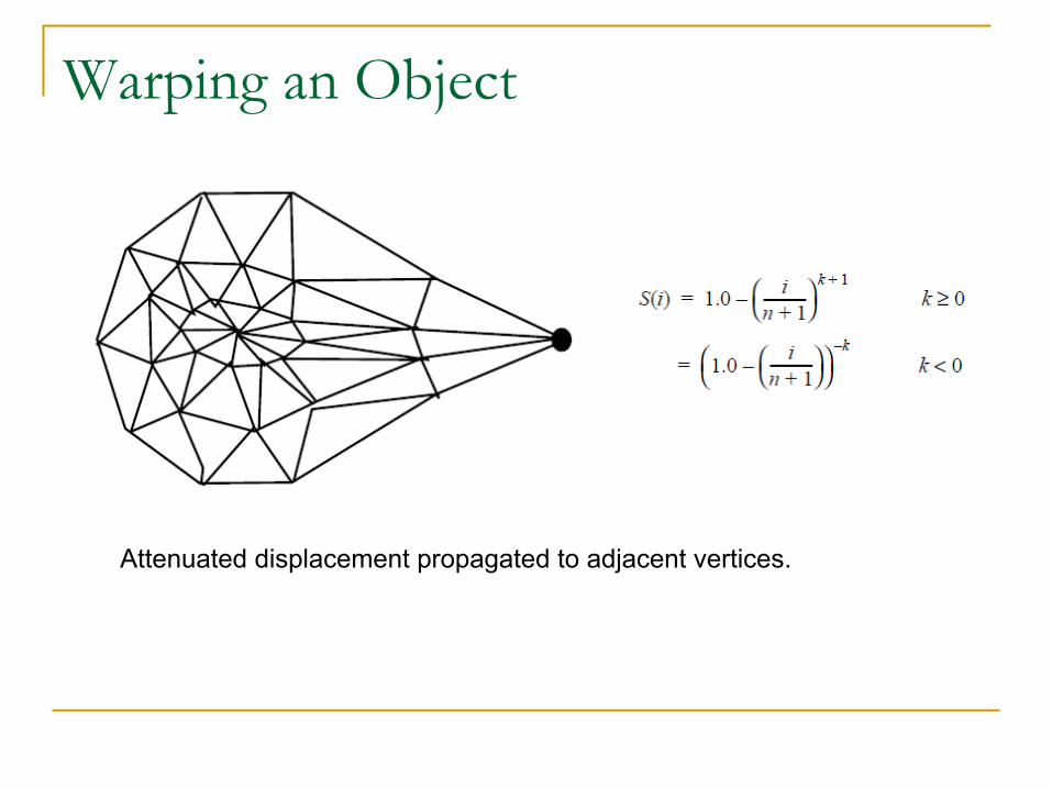
Warping an Object
Attenuated displacement propagated to adjacent vertices.

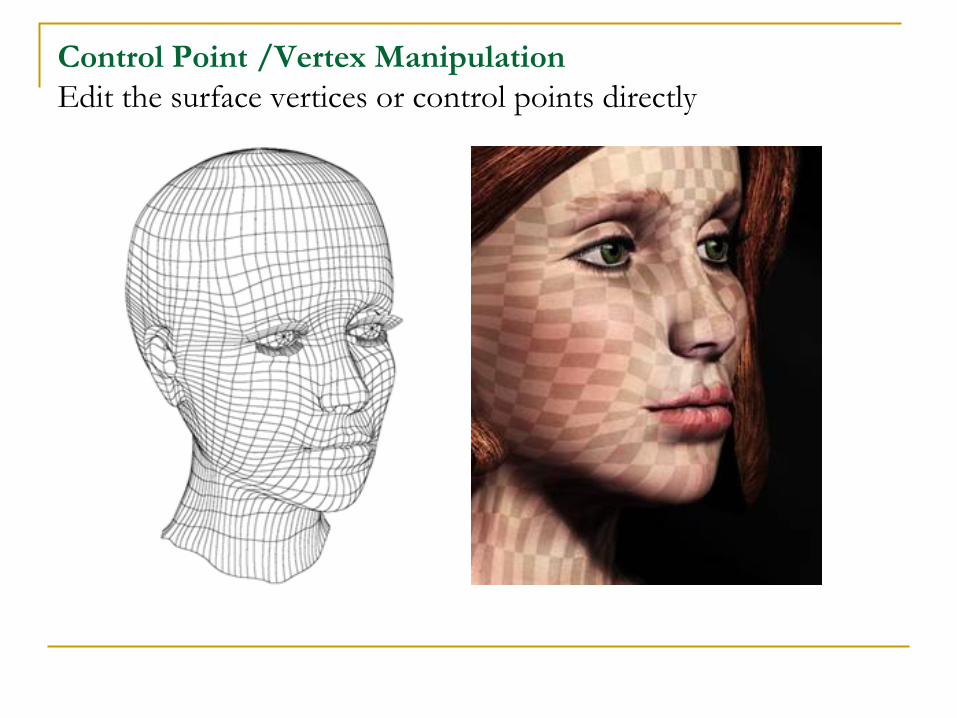
Control Point /Vertex Manipulation Edit the surface vertices or control points directly
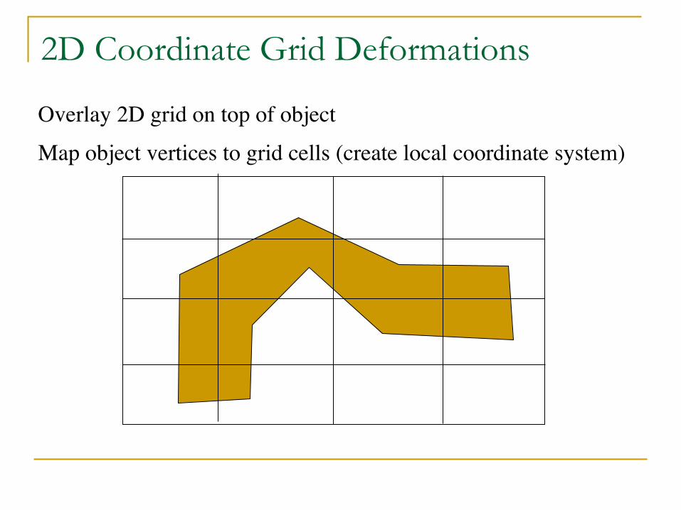
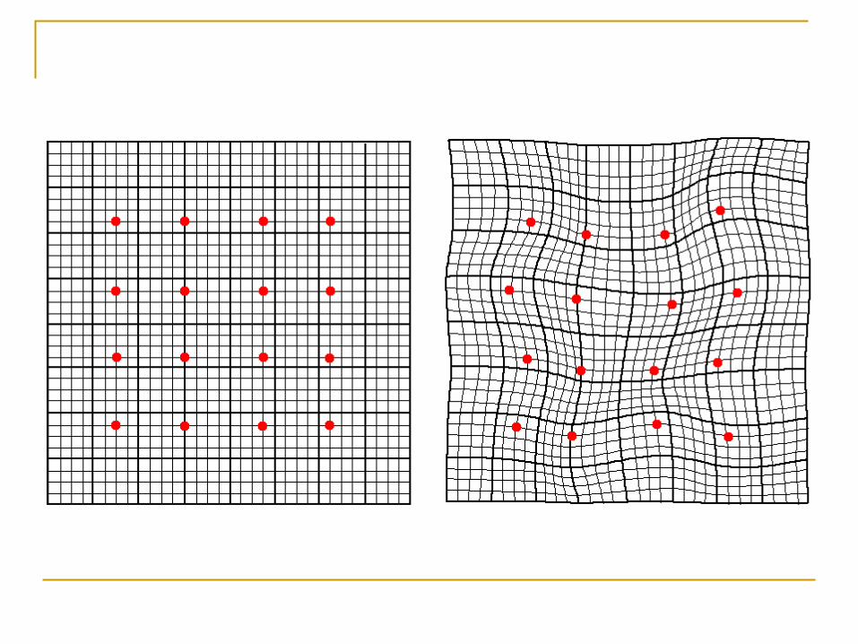
2D Coordinate Grid Deformations
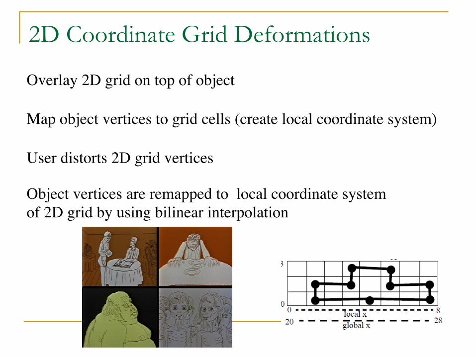
Overlay 2D grid on top of object
Map object vertices to grid cells (create local coordinate system)
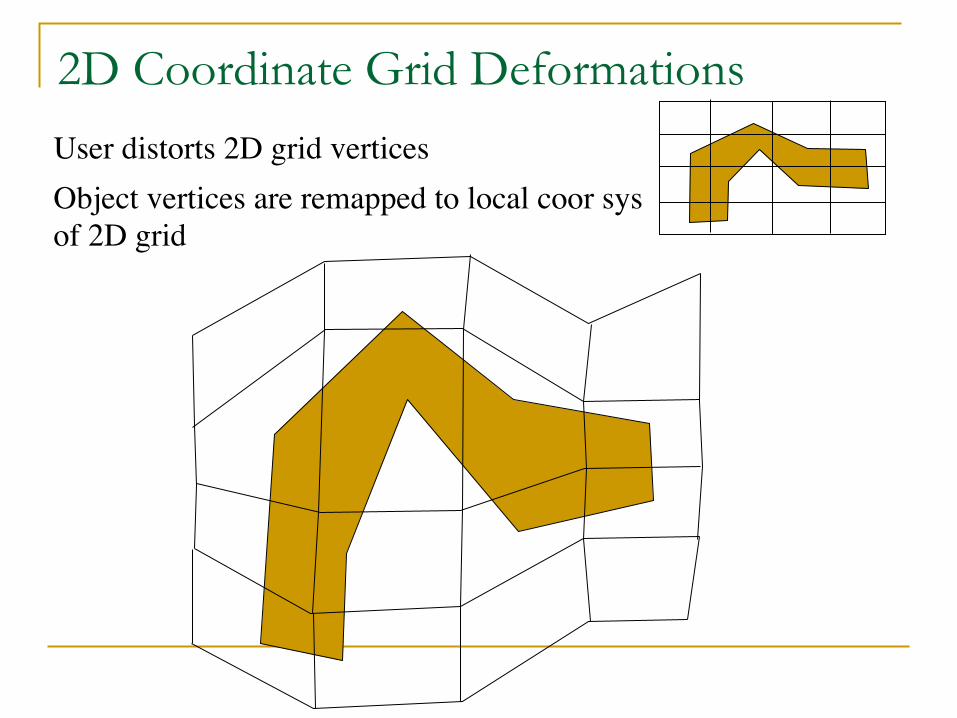
2D Coordinate Grid Deformations
User distorts 2D grid verticesObject vertices are remapped to local coor sysof 2D grid

2D Coordinate Grid Deformations
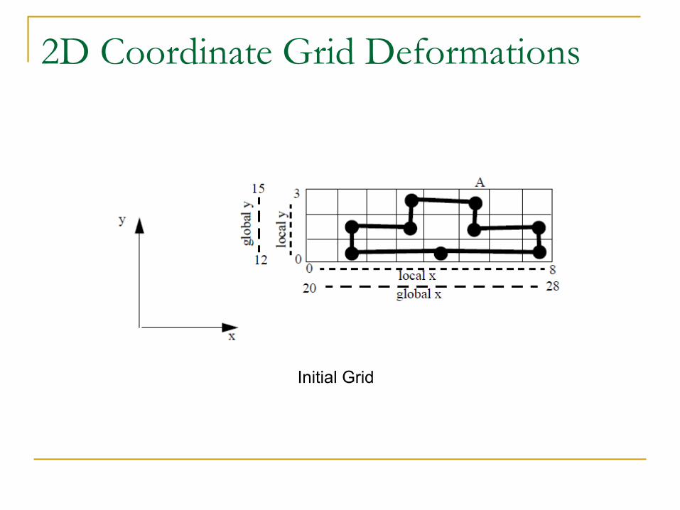
Initial Grid
2D Coordinate Grid Deformations
Overlay 2D grid on top of object
Map object vertices to grid cells (create local coordinate system)
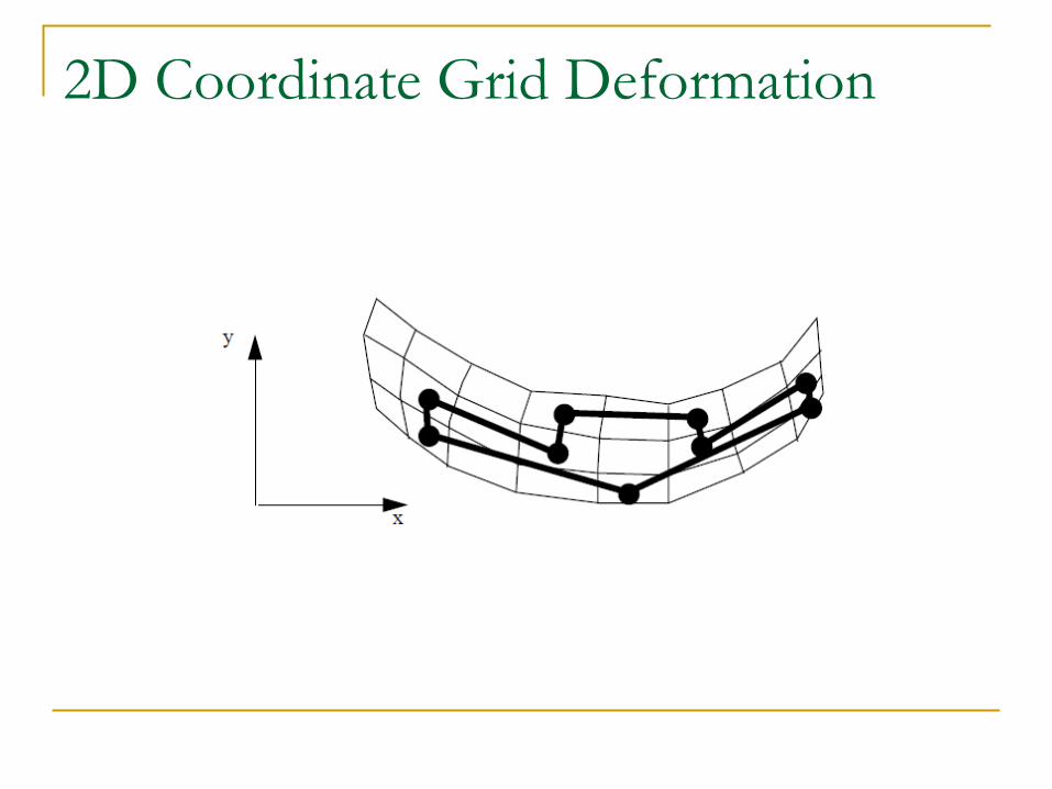
User distorts 2D grid vertices
Object vertices are remapped to local coordinate system of 2D grid by using bilinear interpolation
2D Coordinate Grid Deformations
Initial Grid
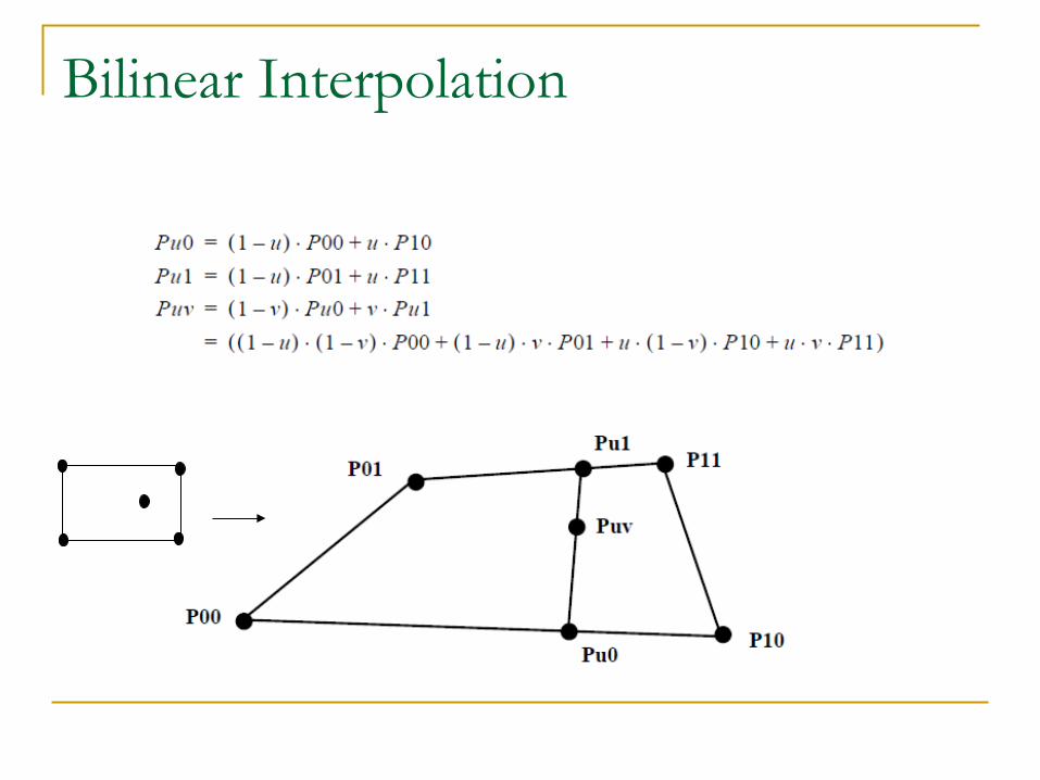
Bilinear Interpolation
2D Coordinate Grid Deformation

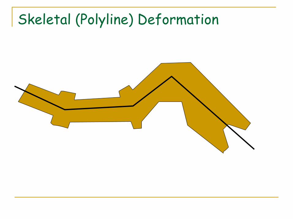
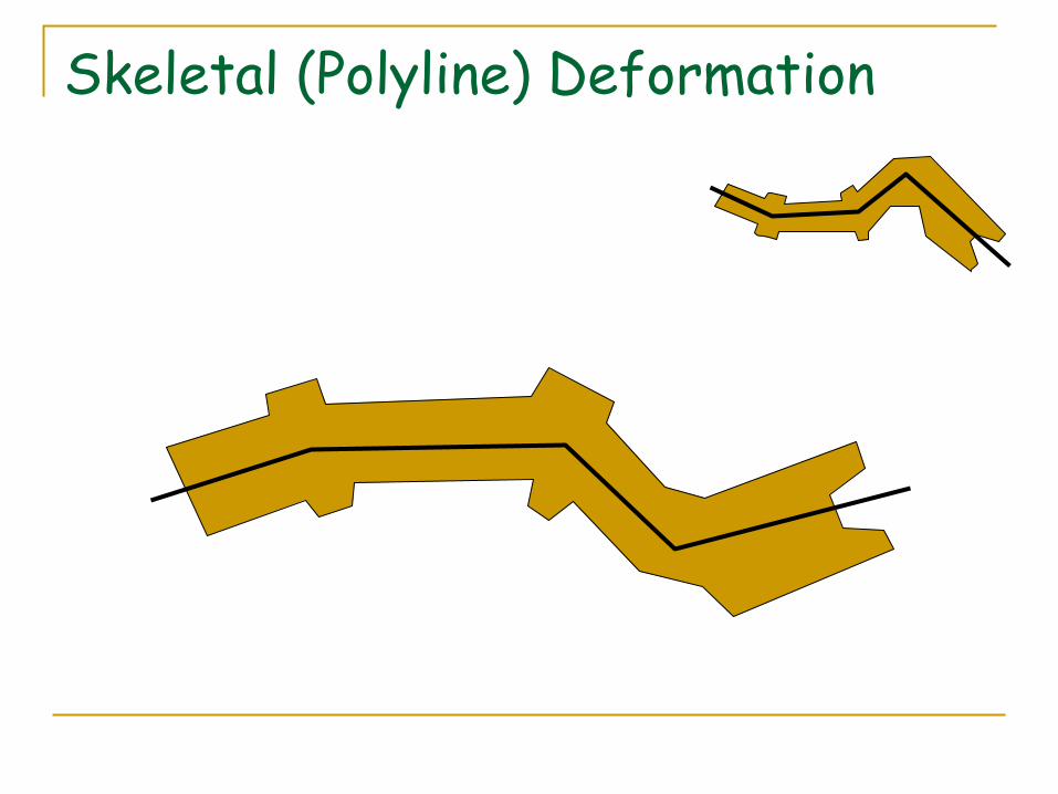
Skeletal (Polyline) Deformation
Skeletal (Polyline) Deformation
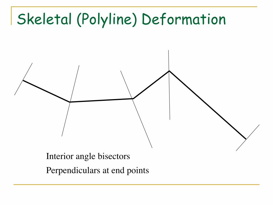
Skeletal (Polyline) Deformation
Interior angle bisectorsPerpendiculars at end points
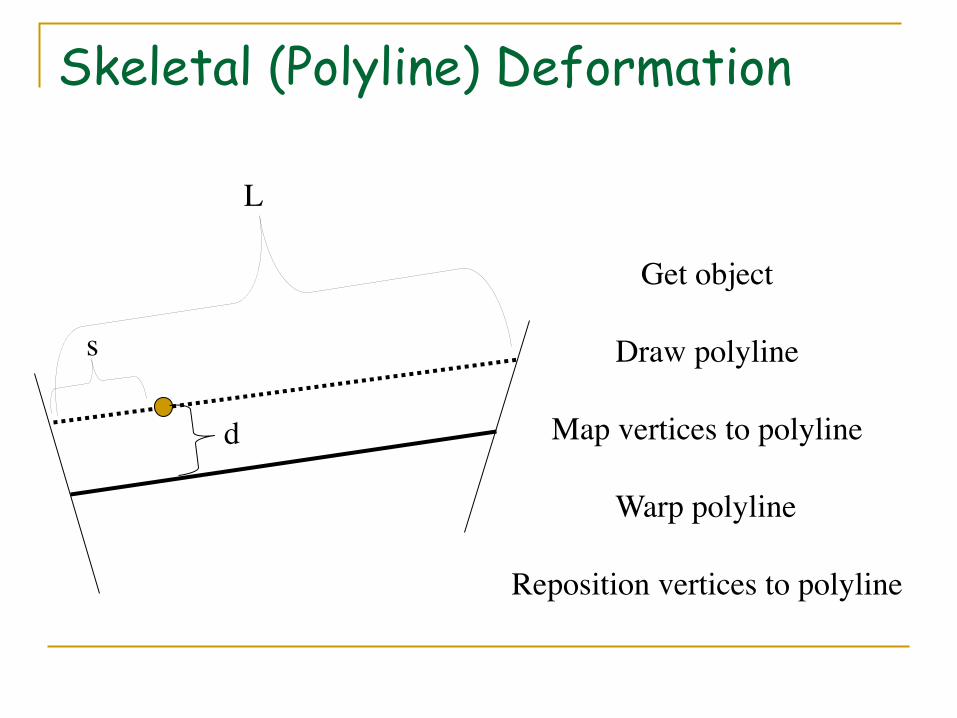
Skeletal (Polyline) Deformation
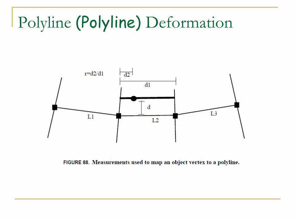
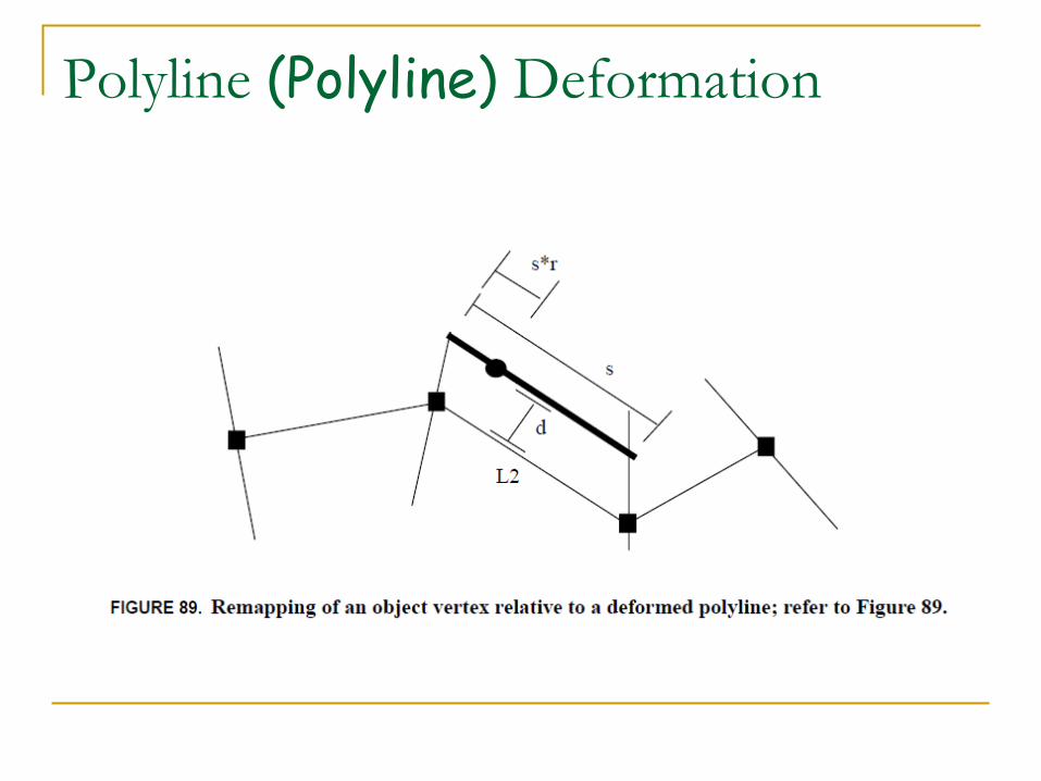
d
L
s
Get object
Draw polyline
Map vertices to polyline
Warp polyline
Reposition vertices to polyline
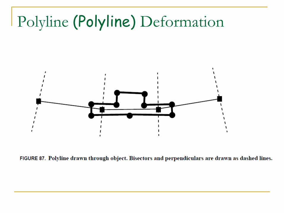
Polyline (Polyline) Deformation
Polyline (Polyline) Deformation
Polyline (Polyline) Deformation

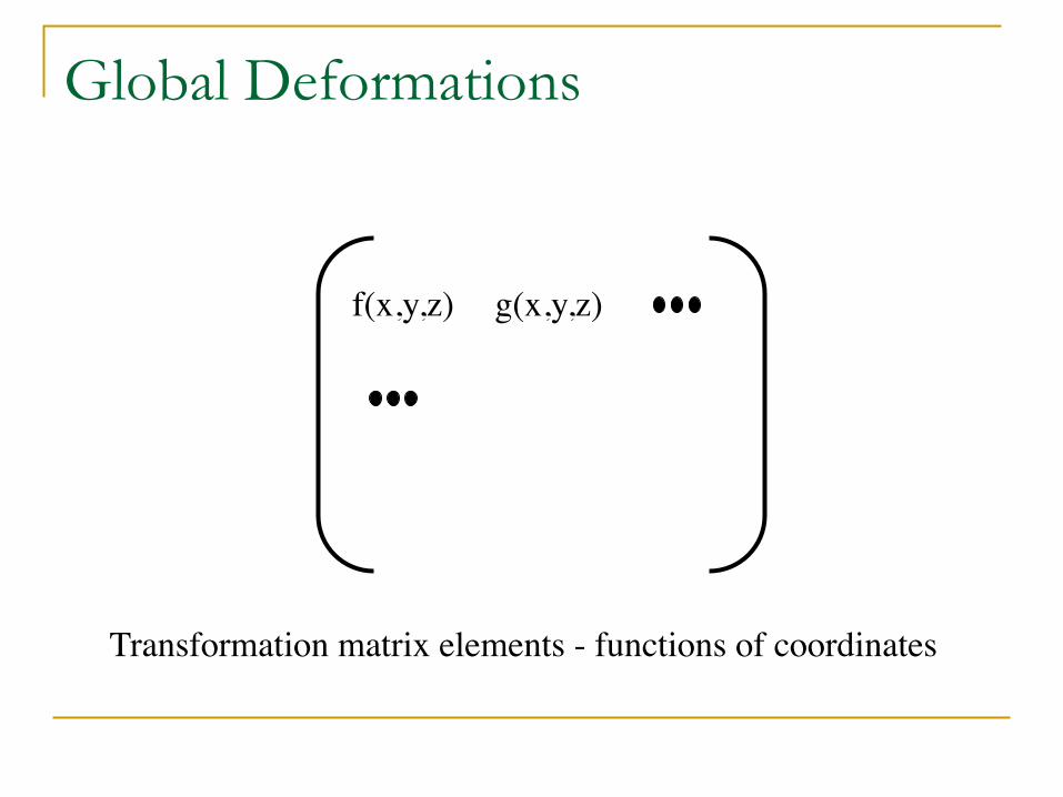
Transformation matrix elements - functions of coordinates
f(x,y,z) g(x,y,z)
Global Deformations
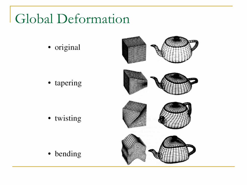
Global Deformation
Global Deformation
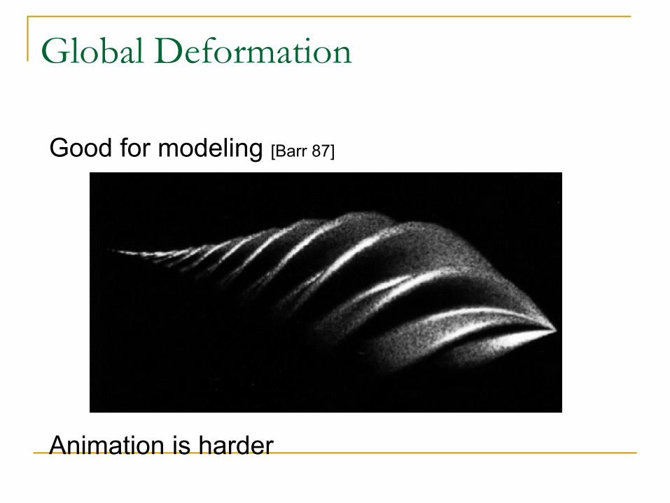
Good for modeling [Barr 87]
Animation is harder
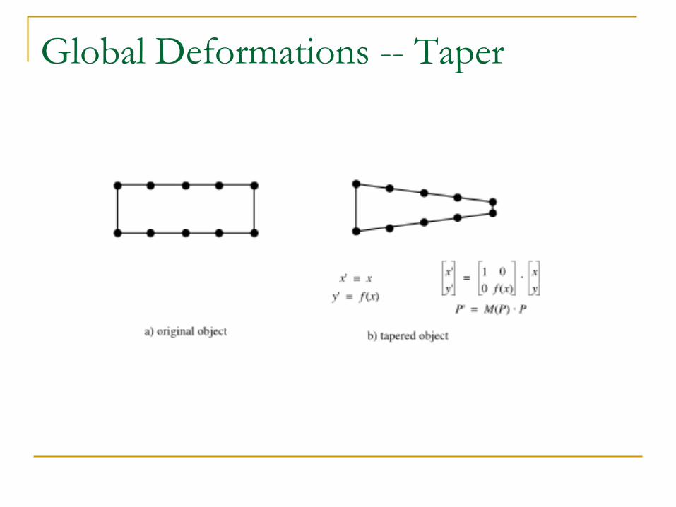
Global Deformations -- Taper
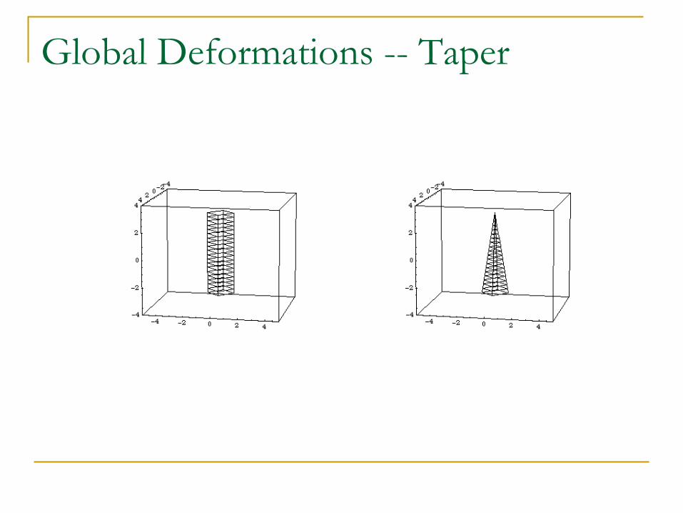
Global Deformations -- Taper
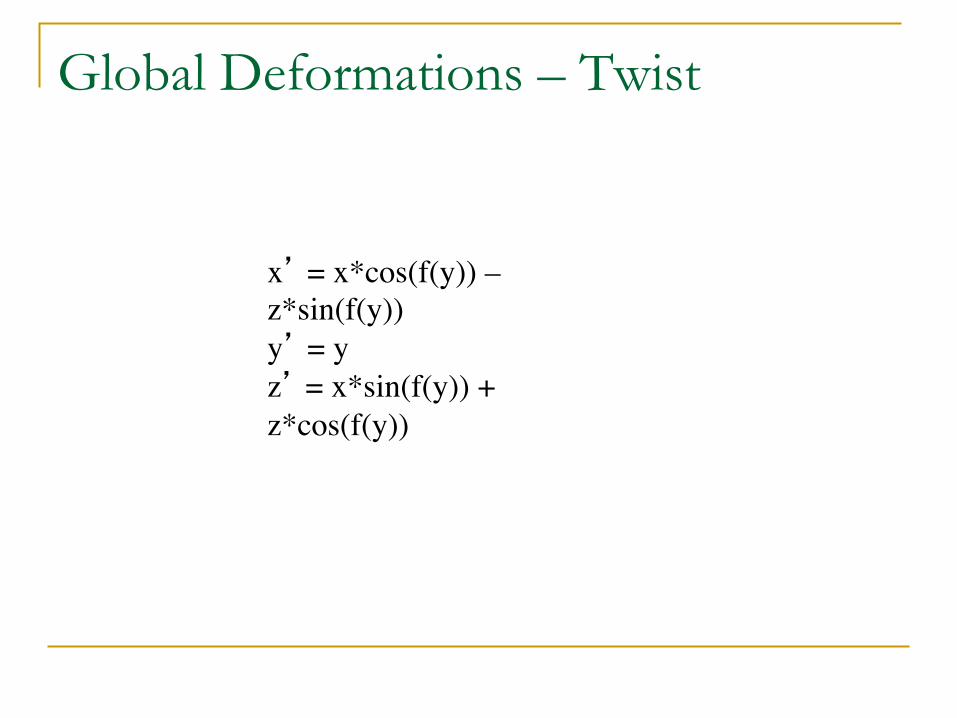
x’ = x*cos(f(y)) – z*sin(f(y))y’ = y z’ = x*sin(f(y)) + z*cos(f(y))
Global Deformations – Twist
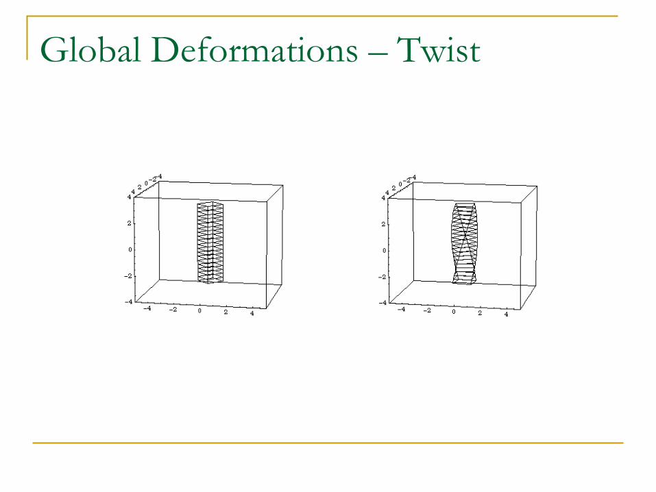
Global Deformations – Twist
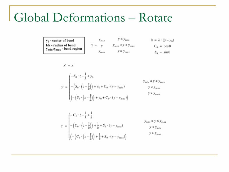
Global Deformations – Rotate
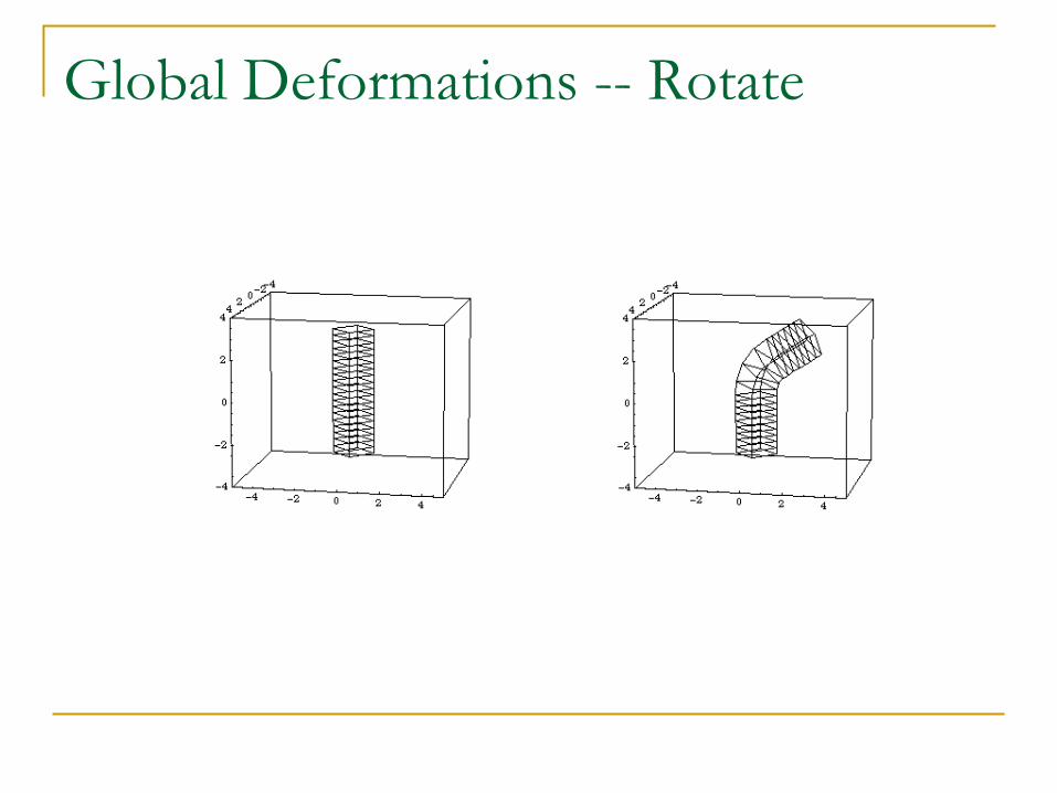
Global Deformations -- Rotate
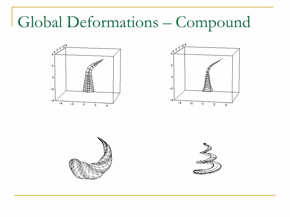
Global Deformations – Compound

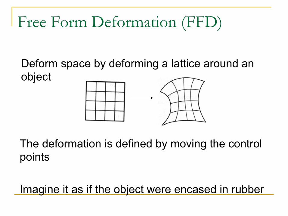
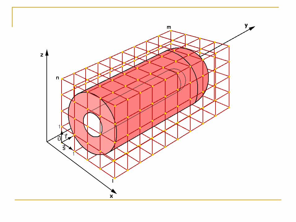
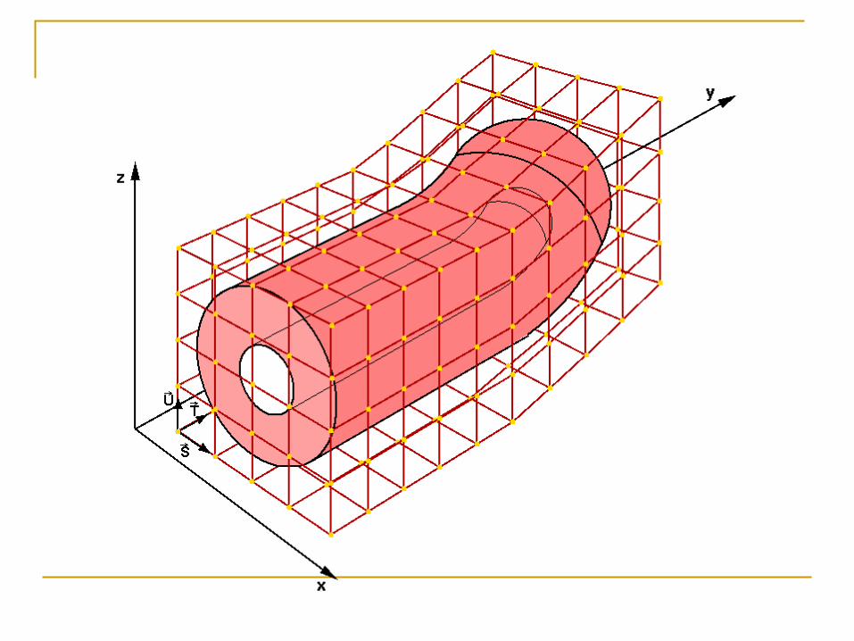
Free Form Deformation (FFD)
Deform space by deforming a lattice around an object
The deformation is defined by moving the control points
Imagine it as if the object were encased in rubber
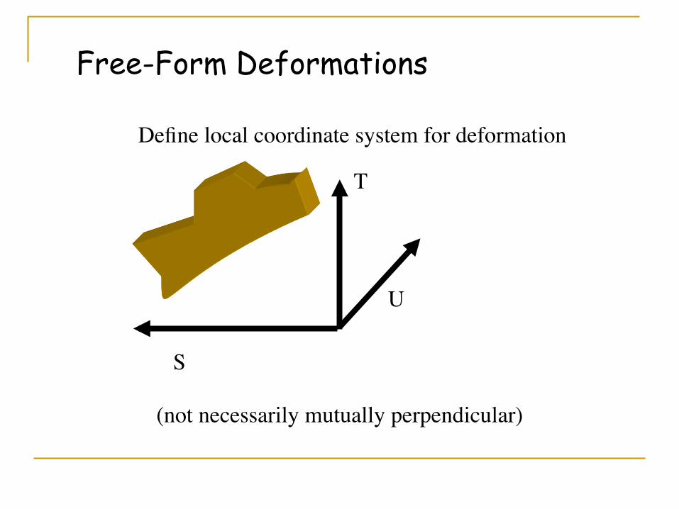
Free-Form Deformations
(not necessarily mutually perpendicular)
S
T
U
Define local coordinate system for deformation
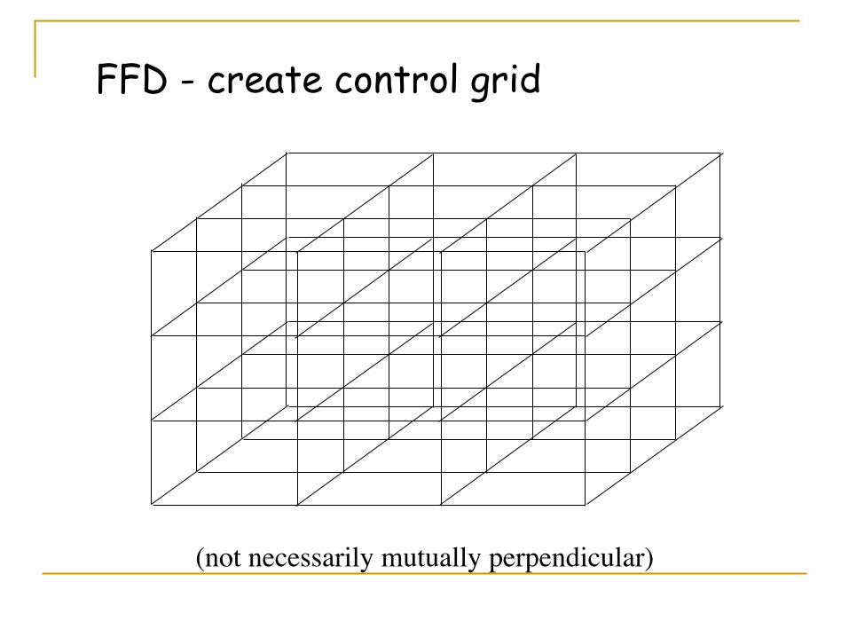
FFD - create control grid
(not necessarily mutually perpendicular)
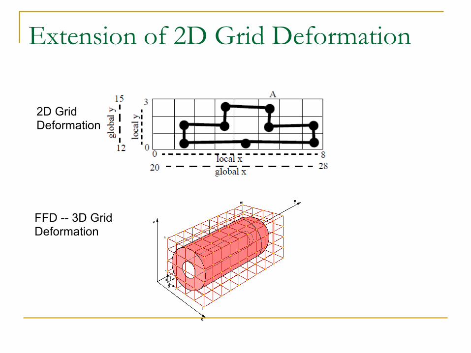
Extension of 2D Grid Deformation
2D Grid Deformation
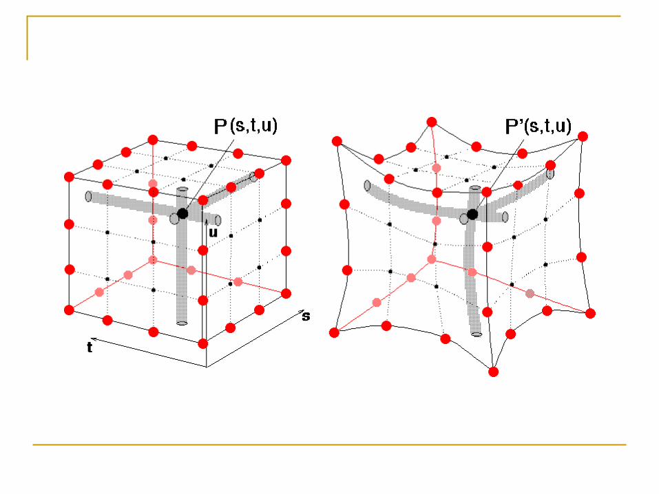
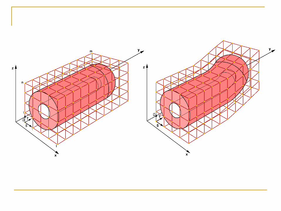
FFD -- 3D Grid Deformation
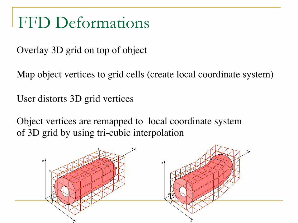
FFD Deformations Overlay 3D grid on top of object
Map object vertices to grid cells (create local coordinate system)
User distorts 3D grid vertices
Object vertices are remapped to local coordinate system of 3D grid by using tri-cubic interpolation
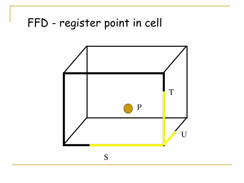
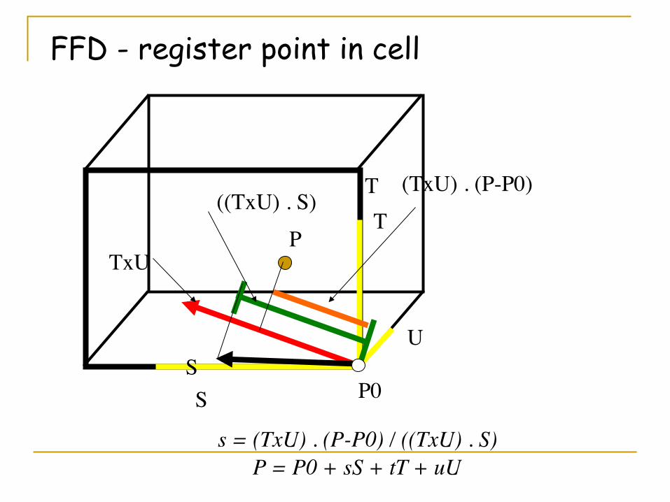
FFD - register point in cell
S
T
U
P
S
T
U
FFD - register point in cell
s = (TxU) . (P-P0) / ((TxU) . S)
TxU
S
T
P
P0
((TxU) . S) (TxU) . (P-P0)
P = P0 + sS + tT + uU
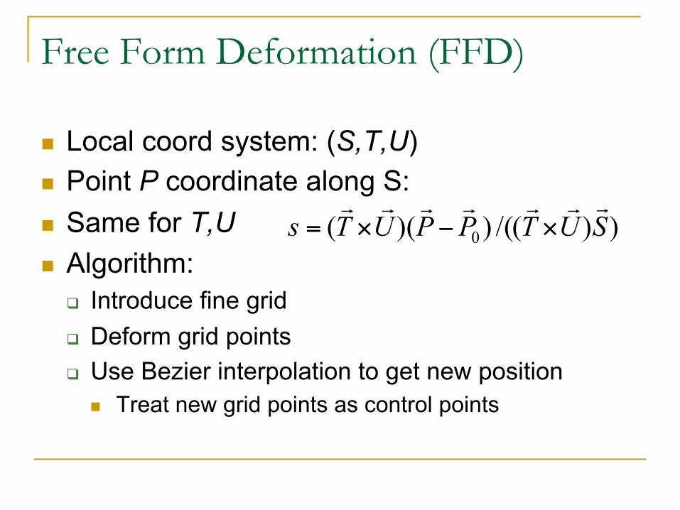
Free Form Deformation (FFD)
n Local coord system: (S,T,U) n Point P coordinate along S: n Same for T,U n Algorithm:
q Introduce fine grid q Deform grid points q Use Bezier interpolation to get new position
n Treat new grid points as control points
))/(())(( 0 SUTPPUTs!!!!!!!
×−×=

Polyline (Polyline) Deformation
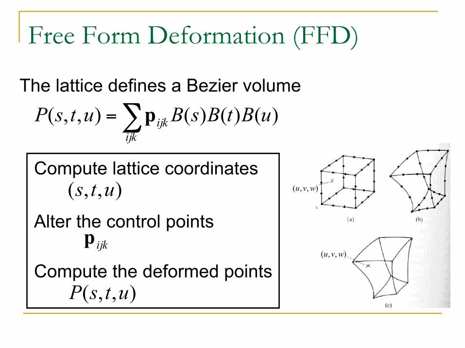
Free Form Deformation (FFD)
The lattice defines a Bezier volume
∑=ijk
ijk uBtBsButsP )()()(),,( p
Compute lattice coordinates
Alter the control points
Compute the deformed points
),,( uts
ijkp
),,( utsP
),,( wvu
),,( wvu
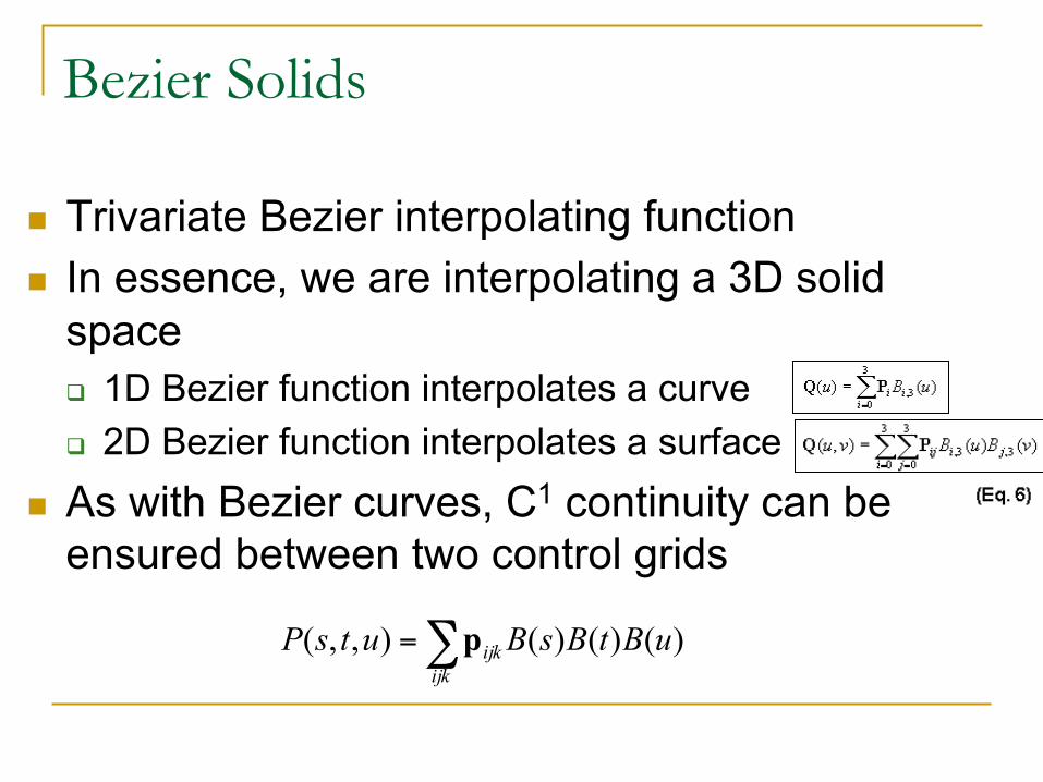
Bezier Solids
n Trivariate Bezier interpolating function n In essence, we are interpolating a 3D solid
space q 1D Bezier function interpolates a curve q 2D Bezier function interpolates a surface
n As with Bezier curves, C1 continuity can be ensured between two control grids
∑=ijk
ijk uBtBsButsP )()()(),,( p
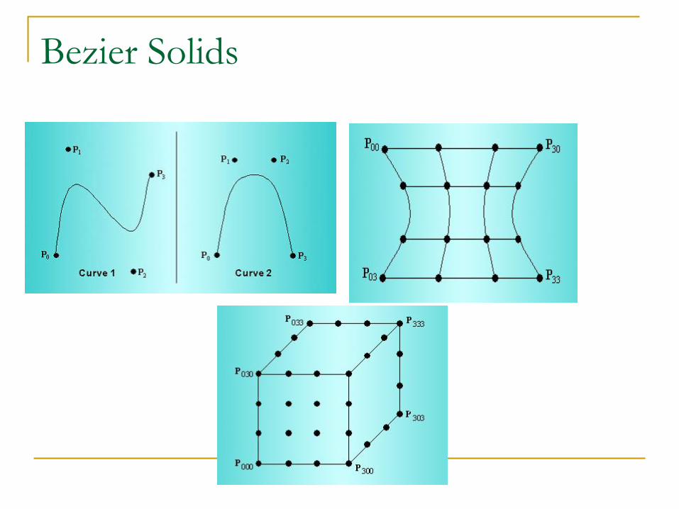
Bezier Solids
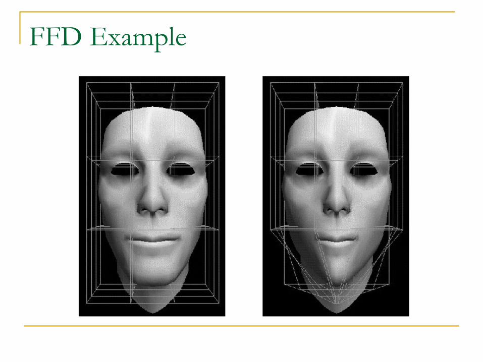
FFD Example
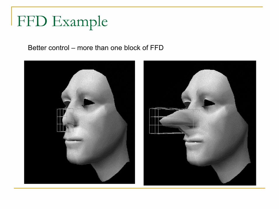
FFD Example
Better control – more than one block of FFD
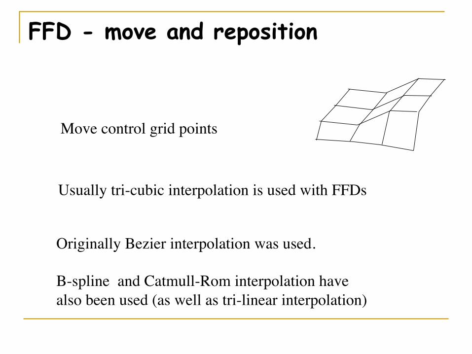
FFD - move and reposition
Move control grid points
Usually tri-cubic interpolation is used with FFDs
Originally Bezier interpolation was used.
B-spline and Catmull-Rom interpolation have also been used (as well as tri-linear interpolation)
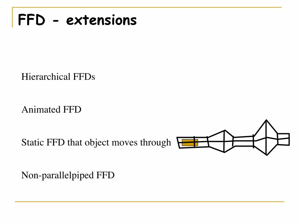
FFD - extensions
Hierarchical FFDs
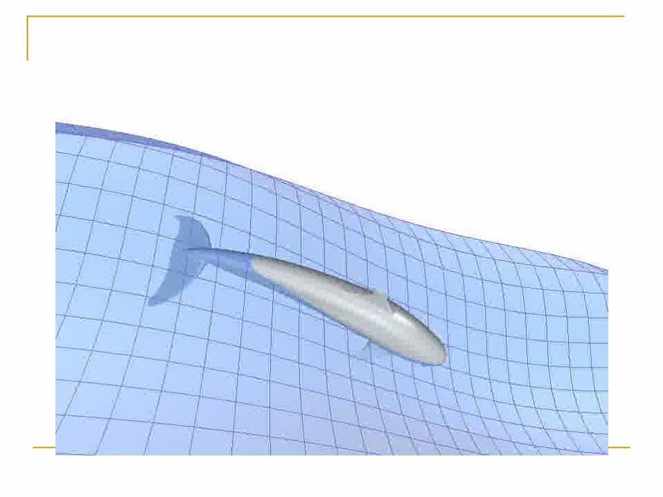
Animated FFD
Static FFD that object moves through
Non-parallelpiped FFD
FFD - films and videos
examples
Boppin’ in Bean Town by John Chadwick
Facit demo by Beth Hofer
Balloon Guy by Chris Wedge
Animation with FFD
n Hierarchical FFD q Coarse level FFD modifies vertices and finer FFD grids
n Moving object through deformation tool q Can move the tool itself
n Modifying control points of FFD q Any technique applies
n Key frame n Physics based
n Example: q FFD is relative to wire skeleton q Moves of skeleton re-position FFD grid q Skin position is computed within new FFD
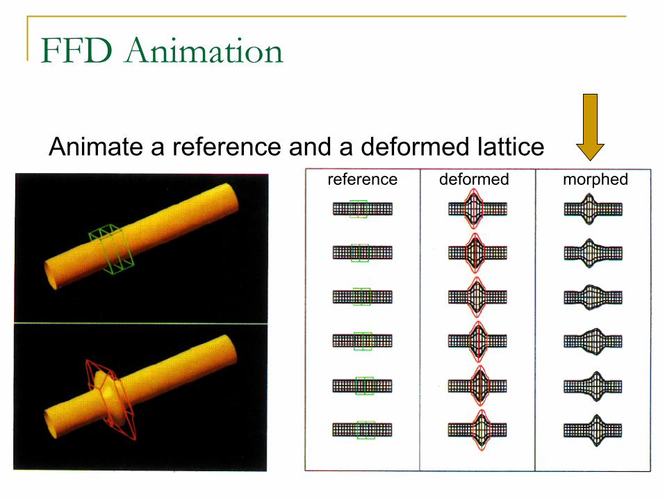
FFD Animation
Animate a reference and a deformed lattice reference deformed morphed
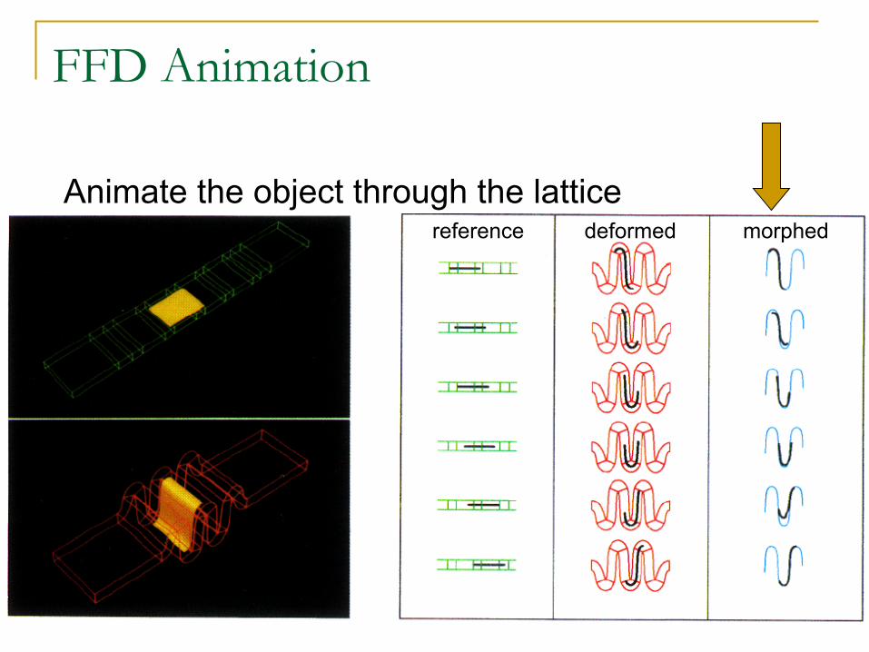
FFD Animation
Animate the object through the lattice reference deformed morphed
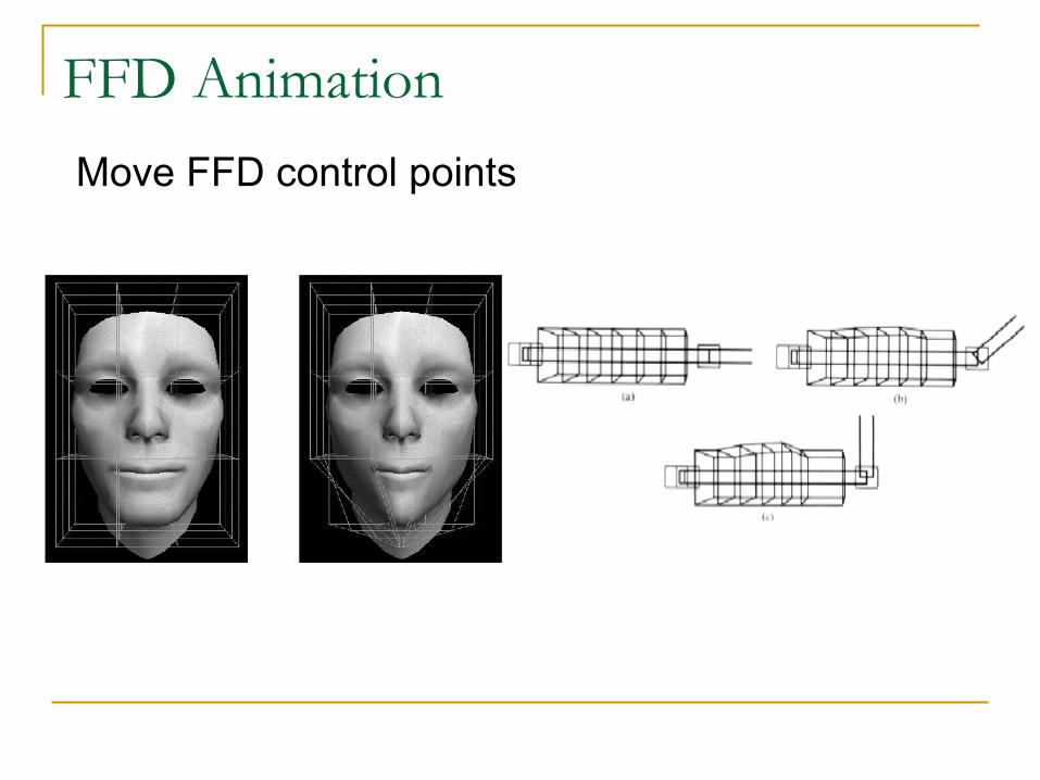
FFD Animation Move FFD control points
A few examples
n https://www.youtube.com/watch?v=kkPUU_VXTAc
n https://www.youtube.com/watch?v=pE8KGVwy2ZI
Next time
n Motion capture n Human animation n Natural phenomena
q Fluids, Smoke etc.
Thanks to Tolga Çapın, for most of these slides