Avoiding Instabilities in Power Electronic Systems: Toward an

On-Chip Implementation

A. Abusorrah$, K. Mandal∗, D. Giaouris†, A. El Aroudi††, M. M. Al-Hindawi$,

Y. Al-Turki$, and S. Banerjee#

$Renewable Energy Research Group, Faculty of Engineering, King Abdulaziz University, Jeddah, Saudi Arabia∗Department of Electrical & Electronics Engineering, National Institute of Technology Sikkim, Ravangla,

South Sikkim - 737139, India, email: dr.kuntal.mandal@gmail.com†School of Electrical and Electronic Engineering, Newcastle University, Newcastle upon Tyne, United Kingdom††The GAEI Research Group, Department d’Enginyeria Electrònica, Elèctrica i Automàtica, Universitat Rovira i Virgili,

43007, Barcelona, Spain#Indian Institute of Science Education & Research Kolkata, Mohanpur Campus, Nadia - 741246, W.B., India

Abstract

The available controller chips for power electronic systems are used for specific transient and steady-state performances. In such

systems, the parameter ranges for stable operation are delimited by slow-timescale as well as fast-timescale instabilities. The

usual practice is to design the control loop based on the state-space averaging technique, which cannot predict the fast-timescale

instabilities. In this paper the first attempt has been made to propose a new design of the controller chip that can suppress these

instabilities, thus extending the stable operating range in the parameter space. For this, we make use of the Filippov method

which can effectively predict both types of instabilities. In this approach, the stability of the system is obtained in terms of

the state transition matrices across each subsystem and saltation matrices across each switching event. The basic idea is to

exercise control over the saltation matrices to increase the stability margin of the periodic orbit. Since in the Filippov approach

an increase in the number of switching events in a cycle does not increase the complexity of the analysis, the proposed controller

chip will be particularly useful in complex power electronic systems such as interconnected converters, multi-input multi-output

converters, resonant converters, micro-grids etc.

Keywords: Stability analysis, Filippov method, saltation matrix, slow-timescale instability, fast-timescale instability, cascaded

converter.

1 Introduction

Controllers for power electronic systems have the specific objective of producing switching signals, which is normally done

using well-established strategies like voltage mode or current mode control. The output voltage is compared with a reference

1

2

voltage to produce the control voltage (in case of voltage mode control) or the current reference for an inner current loop

(for current mode control) using a suitable compensator. The values of the storage elements are set using the information of

maximum allowable voltage and current ripple, and the parameters of the compensator are decided from the consideration of

transient performance using the linearized averaged model of the converter and the standard methods of linear control theory.

These strategies are implemented using analog or digital controllers. The desirable steady-state dynamical behavior is where all

state variables undergo small periodic oscillations at the clock frequency, and EMI filters are designed for that frequency.

Even though these design procedures are well established and universally followed to design converters and controllers,

it has been found that various nonlinear instabilities [1, 2, 3] may set in at different parameter ranges producing undesirable

dynamical behaviors with high current and voltage ripples — like subharmonic oscillations at the clock frequency [4, 5] or a

slow-timescale oscillation at a much lower frequency [6], or even a chaotic oscillation of the state variables [5]. In digitally

controlled converters the discrete sampling and quantization effects can also induce instabilities [7, 8, 9]. The designer therefore

sets the “design limits" of the external parameters (like the input voltage and load) based on the values of these parameters where

such undesirable behavior sets in. These limits are obtained through averaged the model, circuit simulation of the switched

model or experimentally. In complex power electronic systems like cascaded converters, resonant converters, and microgrids,

the available parameter ranges for stable operation can be quite small, due to the interaction between the different stages.

However, to allow larger variations of the parameters, there is a necessity to extend these design limits. For some controllers

specific strategies have been already developed (e.g., the addition of a compensating ramp to the reference signal in current

mode control) to extend these design limits, but these are not general in nature. Therefore, it is necessary to develop methods

of avoiding these nonlinear instabilities that can be applied across different systems and controllers. In [10, 11, 12, 13], some

preliminary work along this line was reported and was applied to the simple dc-dc converter e.g., buck and boost. The purpose

of this paper is to present the approach in a general framework (both theoretically and experimentally) and to provide guidelines

for the design of a controller chip that can implement these ideas. Unlike the existing general chips [14, 15] and application

specific chips [16, 17], the proposed chip will provide the reliable stable operation for larger parameter ranges by tuning the

external resistors proposed controller chip only.

Notable is the fact that the proposed techniques will be effective at steady-state and in no way interfere with targeted transient

performance set by suitable compensator. Moreover, the proposed techniques are different from the chaos control methods

proposed earlier [17] that aim at locating and stabilizing unstable periodic orbits. Our approach is based on the Filippov method,

where the stability of the system is given by the eigenvalues of the monodromy matrix, which is a combination of the state

transition matrices and saltation matrices. By suitable manipulation of the individual components of the saltation matrices,

stability margin of the system can be extended in practice which in turn increase the useful parameter range. All these methods

are validated experimentally in a system of voltage-mode controlled cascaded buck-buck converters.

The rest of the paper is organized as follows. Section 2 presents an overview of stability analysis of periodic orbits using

Filippov method. In Section 3 it has been shown that the instabilities can be controlled by three different techniques, each of

which exercise control over a specific component of the saltation matrix. In Section 4 an example is considered, the voltage-

mode controlled cascaded buck-buck converter, to validate the three specific control methods. The experimental results along

with the implementation circuit diagram with different IC chips for different functions are presented in Section 5. In Section 6,

3

x(0) =x(Ts)

x(t1)

x(t2)

x(tm-1)h2

h1

x

hm-1

f1 f2

fm fm-1f3

(a)x(0)

x(t1)

h1

xf1

f2

n

nTf2

nTf1

x

(b)

x(0) = x(Ts)

x(t1)

h1

x f1

f2

n

(c)

VU

VL t

Vramp

t

tt

CLK

tt

Vcon

Sw

Trailing-edge Dual-edge

(d)

Fig. 1: Schematic diagram of a periodic orbit, switching event and its orientation in a switch-mode converter. (a) Evolutionof the state vector x in the state-space, (b) Enlarged view of switching event h(x, t) = 0, (c) Orientation of switchingsurface when vcon depends on only one state variable (blue) and more than one state variable (black), (d) Different PWMmethods: trailing-edge and dual-edge. (Color online.)

an approach to implement the above ideas in a single controller chip is outlined. Finally in Section 7 the conclusions are listed.

2 Stability analysis of a periodic orbit

As shown in Fig. 1(a), the periodic orbit comprises transitions through a number of subsystems given by different sets of

differential equations, and across switching events. For example, in a simple buck or a boost converter the subsystems are the

ON and OFF conditions of the switch, and the switchings are the transitions from the OFF state to the ON state and vice versa in

continuous conduction mode (CCM). In a more complicated converter like a resonant converter, there may be a large number of

subsystems and switching transitions within a cycle. Subharmonic oscillations or slow-timescale oscillations occur when such

a periodic orbit loses stability. The information about the stability of a periodic orbit is contained in the state transition matrix

computed over a complete cycle. The periodic orbit in continuous time is nothing but the fixed point (x(0)=x(Ts)) in the map

obtained by sampling the state in synchronism with the clock period Ts. The state transition matrix computed over a complete

cycle is nothing but the Jacobian matrix of the map computed at the fixed point. If the magnitude of all the eigenvalues of this

matrix are below 1, the periodic orbit is stable.

According to the Filippov approach, the state transition matrix across a full cycle (also called the monodromy matrix) can be

calculated as a product of the state transition matrices across each subsystem (denoted as Φi, where i identifies the subsystem)

4

and the state transition matrices across the switching events called saltation matrices (denoted as Si,j for transition from the ith

subsystem to the jth subsystem). Thus an orbit that goes through m subsystems, the monodromy matrix can be written as

Φcycle = Φm · Sm−1,m ·Φm−1 · · ·Φ2 · S1,2 ·Φ1 (1)

Most power electronic systems are composed of linear subsystems. In that case the state transition matrices across the subsystems

are given by exponential matrices

Φi =eAit

where Ai is the state matrix for the ith subsystem.

Now let us consider the state transition matrix across switching events. Suppose there is a switching causing transition from

the ith subsystem to the jth subsystem when a condition h(x, t)=0 is satisfied. For example, if the switching occurs when the

control voltage equals a ramp waveform voltage, i.e., vcon − vramp = 0, then the switching function h(x, t) is vcon − vramp.

Suppose that the state equations for the two subsystems are given by

Subsystem i: x =f i(x, t)=Aix + Biu (2)

Subsystem j: x =f j(x, t)=Ajx + Bju (3)

Then the saltation matrix across the switching event is given by [18]

Si,j = I +(f j − f i)n

>

n>f i + ∂h/∂t(4)

where I is the identity matrix of the same order as the number of state variables, h(x, t)=0 represents the switching condition

which defines a hyper surface in the state-space of the system, n is the vector normal to the switching surface, and n> is its

transpose. Some of the components of the saltation matrix are shown in Fig. 1(b).

The switching conditions can be of two types:

(a) state-induced switching, where switching occurs when some condition on the state variables is satisfied (for example, the

inductor current reaching a reference value), and

(b) time-induced switching, where switching occurs when some condition on time is satisfied (e.g., turning the switch on

periodically).

The expression (4) gives the state transition matrix for state-induced switching transitions. For time-induced switching the Si,j

matrix is unity [10]. The periodic orbit becomes unstable when any of the eigenvalues of the matrix Φcycle goes out of the unit

circle. This can happen in three different ways:

• if an eigenvalue becomes equal to −1, a subharmonic oscillation sets in;

• if an eigenvalue becomes equal to +1, a saddle-node bifurcation happens; and

5

• if a pair of complex conjugate eigenvalues has a magnitude of unity, a slow-timescale oscillation sets in.

3 Control of instabilities using saltation matrix

At first, it is to be noted that the matrix Φcycle that ultimately decides the stability of the orbit is composed of two types of

component matrices: the state transition matrices Φi along the subsystems, and Si,j for transitions across subsystems. We now

focus on each one, individually.

The current practice of power electronic design is aimed at deciding the parameter values that appear in the state matrices Ai.

These include the values of the inductances, capacitances, the compensator parameters, etc. We propose to keep these design

procedures unaffected, and so do not aim at making any alteration in the state transition matrices Φi. This ensures that the ripple

magnitudes and the transient performance—aimed at which the controller was designed—remains unchanged.

Our proposed techniques focus on making small alterations in the matrices Si,j to push the eigenvalues of the monodromy

matrix inside the unit circle. Since the state transition matrix across a time-induced switching transition is an identity matrix, it

is further narrowed down on the events of state-induced switching.

Upon a closer examination of the expression (4) it has been noticed that it is composed of the following components:

f i,f j : the RHS of the state equations before and after switching

n : the vector normal to the switching surface

∂h/∂t : the rate at which the switching surface h(x, t) moves with respect to time

Out of these, f i (or Ai and Bi) and f j (or Aj and Bj) contain the design parameters, which were decided to leave unaltered.

Therefore, the control of instabilities can be affected by the remaining two components, ∂h/∂t and n. In the following sections

we illustrate various ways in which these two can be altered, and in a given situation any of these possibilities can be adopted

depending on the preference of the designer.

3.1 Controlling the normal vector n

The normal vector depends on the orientation of the switching surface in the state space as illustrated in Fig. 1(c). Consider a

voltage mode controlled buck converter with a proportional controllerKp. The control voltage vcon =Kp(Vref−vo) is dependent

on the output voltage alone. Therefore, in the capacitor voltage versus inductor current state space, h(x, t) = vcon−vramp will

be a straight line parallel to the inductor current axis for an ideal capacitor (ESR=0). The vector n normal to that is parallel to

the voltage axis. Due to the time-variation of vramp, the function h sweeps through the state space, and switching occurs when

it meets the state-point.

It is clear that, so long as the control voltage is generated through capacitor voltage feedback alone, the orientation of the

switching function h will be the same (shown by blue color). If the inductor current iL is also used to generate the control signal

vcon, the orientation of h will change (shown by black color) and the expression of vcon becomes as follows:

vcon =Kp(Vref − vo) −KiLiL

where KiL is the gain for current feedback. If a proportional-integral (PI) controller is used for the voltage loop together with

6

current feedback, the expression becomes

vcon =Kp(Vref − vo) +Ki

∫(Vref − vo)dt−KiLiL

where Ki is the integrator gain. The integrator has an associated state variable ρ=∫

(Vref − vo)dt. The new switching surface is

h(x, t)=vcon−vramp =Kp(Vref − vo) +Kiρ−KiLiL−vramp

Therefore, the normal vector to the switching surface is given by

n=

∂h/∂vo

∂h/∂iL

∂h/∂ρ

=

−Kp

−KiL

Ki

By controlling the ratio ofKp andKiL , the normal vector can be controlled. This approach is particularly applicable in situations

where the current signal is available in the voltage across the capacitor, because of the ESR of the capacitor [19].

3.2 The control of ∂h/∂t

In case of pulse-width modulation techniques, the switching surface sweeps through the state space. For example, in a voltage

mode controlled converter, the switching occurs when the control voltage equals the ramp voltage:

h(x, t) = vcon − vramp

= vcon −VL + (VU − VL)

(t

Tsmod 1

)(5)

The expression (5) shows that the time-dependence of h depends on both the control voltage and the ramp voltage. The lower

and upper thresholds of the vramp are denoted by VL and VU respectively and Ts is the clock period.

3.2.1 Slope control of vramp

In a voltage mode controlled converter, the switching surface h(x, t) sweeps through the state space at a speed of

∂h

∂t=−VU − VL

Ts

This is nothing but the slope of the ramp waveform. This slope can be altered by making small changes in (VU − VL) while

keeping the clock period constant, or by varying the clock period Ts while keeping amplitude of the ramp signal constant. The

second option may not be desirable because the EMI filters are tuned to the clock frequency.

It is interesting to note that in current mode control, the widely known technique of adding a stabilizing ramp achieves

exactly this, as it induces a change in ∂h/∂t. In this paper we are generalizing the idea, to make it applicable to any converter

and control strategy.

7

3.2.2 Addition of external signal with vcon

Normally the control voltage is generated through a linear compensator using the feedback of the output voltage and eventually

the inductor current that needs to be regulated. Therefore vcon does not have any explicit dependence on time. But the injection

of a time-varying signal can make vcon explicitly dependent on time, which can act as a lever in controlling ∂h/∂t.

An interesting possibility is offered by the injection of a sinusoidal signal synchronized with the clock frequency fs (or at an

integer multiple of the clock frequency). It has been shown earlier that this strategy can effectively increase the parameter range

for stable operation [12, 10]. Suppose that the injected signal is given by q(t)=a sin(ωst+ θ) where ωs =2πfs. In order to be

used as an effective stabilization strategy, the design guideline has to take into account the following considerations. Firstly, this

injected signal is not likely to be invasive of the desired steady-state operation and therefore to alter the duty ratio in the steady

state. Therefore its value should be zero at the switching instant, i.e.,

sin(ωst+ θ)=0 at the switching instant

or, θ=−2π×dwhere d is the duty ratio. The steady state duty ratio can be calculated using the information about the input voltage

and the demanded output voltage, which can be used to set the phase of the injected sinusoidal signal. Secondly, a maximum

effect on ∂h/∂t at the switching instant is desired. This is automatically guaranteed if the injected signal is a sinusoid, because

the derivative is a cosinusoid, which assumes a maximum value when the signal itself has zero value.

3.2.3 Utilizing the edges of triangular wave

Fig. 1(d) shows two different PWM modulation methods: trailing-edge and dual-edge which can give different stability margins.

If a ramp waveform with an instantaneous reset (trailing-edge) is used to generate the PWM, the first switching within a clock

cycle is a state-dependent switching and the second one is time dependent. Thus, saltation matrix across the second switching

is always an identity matrix. But if the trailing edge of the waveform does not drop instantaneously and goes through a steady

decline with a definite slope (dual-edge), one can have state-dependent switching there also. Thus there would be a non-identity

state transition matrix at the second switching event within a clock cycle, and that would have an effect on Φcycle, which can be

used to push the eigenvalues into the unit circle. Note here that the number of subsystems within a switching cycle increases and

the dynamics of the overall system will change. This fact has to be taken into account when designing the controller.

In all practical analog implementations, the trailing edge of the PWM waveform is generated by discharging a capacitor—

which cannot happen instantaneously. Therefore, to implement the proposed strategy, all that one has to do is to enforce a

state-dependent switching. In digital implementations, the sampling must be done when there is no ringing noise and the easiest

way to implement this is by changing the ramp waveform to a triangular wave (dual-edge).

4 Example: Cascaded Buck-Buck Converter

Cascaded converters are used in many applications such as telecommunication systems, computers, and military applications

(space stations, aircraft, ships) [20]. It has flexible configuration, high efficiency, and reduced weight and size. Many criteria have

been proposed [21] to analyze the stability of such systems, e.g., impedance criterion, phase margin and gain margin criterion,

8

the opposing argument criterion, the energy source analysis, the maximum peak criterion. [22, 23] have shown, with counter-

examples and case studies, that these methods are not applicable to all power electronic systems in general. Some alternate

stability assessment methods are also available [24, 25, 26]. However, in these methods the switching dynamics implicitly

appear in the expressions, and so these are difficult to apply in complex systems with a large number of switching in a cycle.

The proposed techniques in this paper have been illustrated with a cascade connection of two buck converters which is used in

applications that require a low output voltage. More specifically there is a standard voltage mode controlled buck converter with

PI compensator followed by another one as shown in Fig. 2(a). Unlike the approximate linearized state-space averaged model

which neglects the switching dynamics, we have used an exact model of the overall switched nonlinear system considering the

interaction between two stages.

So far most of the research on cascaded converters has been done for the converters operating in continuous conduction

mode (CCM), feeding constant power loads (CPLs). In this paper, a system is considered in which the first converter operates

in discontinuous conduction mode (DCM) and the second in CCM—a configuration on which very few reports are available

[27, 28]. In this system there are 8 subsystems, and there can be many switching events within a clock cycle. Such a system

is very difficult to analyze using the methods mentioned earlier. But in our approach, the complexity of the system does not

increase the complexity of the model.

4.1 System Description

As shown in Fig. 2(a), both the switches S1 and S2 are driven by pulse-width modulated (PWM) switch signals u1 and u2.

These signals are generated by comparing the control voltage vcon with a ramp signal vramp. When vcon is greater than vramp,

the switch signal u is “HIGH" and is “LOW" otherwise. The PI compensators are used to get zero steady-state error for both the

output voltages. To prevent multiple switching within a clock cycle S-R flip-flops (FF1 and FF2) have been introduced.

For the first converter, the control voltage and the ramp voltage are given by

vcon1 =Kp1(Vref1 − vo1) +Ki1

∫(Vref1 − vo1)dt

vramp1 =VL1 + (VU1 − VL1)

(t

Tsmod 1

)

where, Kp1 and Ki1 denote the proportional and integral gains respectively, vo1 is the output voltage, VL1 and VU1 are the

threshold voltages of the ramp, and Ts is the switching period.

4.2 Mathematical Modeling

The power stage of the system (Fig. 2(a)) is described by the following set of differential equations

diL1

dt=

1

L1[−vo1 + u1Vin] ,

dvo1

dt=

1

C1[iL1 − u2iL2 ] , (6)

diL2

dt=

1

L2[u2vo1 − vo2] ,

dvo2

dt=

1

C2

[iL2

− vo2

RL

](7)

where u1 =1 and u2 =1 if both the switches S1 and S2 are ON (u1 =0 and u2 =0 if S1 and S2 are OFF).

9

+−

Vin

C2 RL

S2S1

D1 D2 vo2

iL1

+-

L1 L2vo1C1

+-

Vref1+ -

vcon1

VU1

VL1t

vramp1

iL2

S

R

Q CLK1

+ -Vref2

+ -

vcon2

VU2 tvramp2

S

R

Q CLK2

+ -VL2

Kp1 ,Ki1 Kp2 ,Ki2

FF1 FF2

u1 u2

(a) (b)

(c) (d)

Fig. 2: Cascaded buck-buck converters with voltage mode control (a) Closed-loop circuit diagram, (b) Nominal period-1 wave-forms of the control voltages, ramps, and currents when the first converter is in DCM and the second converter is inCCM, (c) Stable region in the Kp1−Kp2 parameter space with Vin =24 V, RL =5 Ω, (d) Stable region in the Vin −RL

parameter space with Kp1 =Kp2 =2. Other parameters are given in Table 2(b).

The two integrators of the PI compensatots are given by the following state equations

dρ1

dt=Ki1[Vref1 − vo1],

dρ2

dt=Ki2[Vref2 − vo2]. (8)

For different operating conditions there are different switch signals u (subsystems Mk) as given in (Table 1). For two switches

(S1 and S2), 22 different set of linear differential equations are possible in continuous conduction mode (CCM). In discontinuous

conduction mode (DCM) of the first stage (iL1= 0, both S1 and D1 are OFF), the number of subsystem increases by four

(Table 1).

Table 1: Status of switch signals and different subsystems in CCM and in DCM of the first stage

u2 u1 iL1Mk u2 u1 iL1

Mk

0 0 >0 M0 0 0 0 M4

0 1 >0 M1 0 1 0 M5

1 0 >0 M2 1 0 0 M6

1 1 >0 M3 1 1 0 M7

As shown in Fig. 2(b), when the first stage is in DCM there are four subsystems (M3−M1−M0−M4) within a switching cycle

(or clock period) for a typical steady-state operation.

10

Each subsystem is represented using state-space model as

Mk : x = Ak x + Bk u

where, x =[iL1 vo1 ρ1 iL2 vo2 ρ2

]>, u =

[Vin Vref1 Vref2

]>. The subsystems Mk are defined in Table 1 and some of them

are appearing in a typical steady-state are shown in Fig. 2(b).

The transitions between subsystems occur after satisfying switching conditions which change the status of the switch signals.

Therefore, the switching instants can be determined from the following switching conditions:

h1 : vcon1 − vramp1 = 0, h2 : vcon2 − vramp2 = 0, h3 : iL1= 0.

Table 2: System design: (a) Specifications, and (b) Parameter values for power-stage and controllers.

Specifications ValuesInput voltage Vin =24 V

Output voltage (1st stage) vo1 =12 V±5%Output voltage (2nd stage) vo2 =5 V±1%

Output Power Po2 =5 WSwitching frequency fs =10 kHz

(a)

Parameters ValuesInductors L1 =0.70 mH, L2 =1.5 mHCapacitors C1 =50 µF, C2 =50 µF

Output Resistor RL =5 ΩVoltage References Vref1 =12 V, Vref2 =5 V

Threshold of the ramps VU1 =VU2 =2.5 V, VL1 =VL2 =−2.5 VProportional gains Kp1 =Kp2 =2

Integral gains Ki1 =Ki2 =1000 s−1

(b)

4.3 Design of the Overall System

Based on the specifications (Table-2(a)), the design values of the power-stage and controllers are given in Table-2(b). The current

ripple in the second stage is kept within ±20% of the output current.

(a) (b) (c)

Fig. 3: Bifurcation diagram and waveforms. (a) Bifurcation diagram with Vin as varying parameter, (b) waveforms at Vin =20 V,slow-time-scale or quasi-periodic oscillations, (c) waveforms at Vin = 30 V, subharmonic oscillation. Other parametersare given in Table 2(b).

11

Table 3: Eigenvalues for different values of Vin corresponding to Fig. 3(a).

Vin(V) Orbit Subsystem Sequence Eigenvalues20.00 Unstable Period-1 M3−M1−M0 0.1860 ± 0.9879j (≈ 1.0053), 0.5590 ± 0.6395j, 0.9561, 0.961723.32 Unstable Period-1 M3−M1−M0 0.1012 ± 1.0028j (≈ 1.0078), 0.5566 ± 0.6391j, 0.9553, 0.961823.33 Stable Period-1 M3−M1−M0−M4 0.9572 ± 0.0048j (≈ 0.9572), 0.5553 ± 0.6119j, 0.1407, 024.00 Stable Period-1 M3−M1−M0−M4 0.9571 ± 0.0045j (≈ 0.9571), 0.5556 ± 0.6127j, 0.1121, 026.90 Stable Period-1 M3−M2−M0−M4 −0.9995, 0.5709 ± 0.6074j (≈ 0.8336), 0.9555, 0.9541, 026.91 Unstable Period-1 M3−M2−M0−M4 −1.0002, 0.5708 ± 0.6074j (≈ 0.8335), 0.9555, 0.9541, 026.91 Stable Period-2 M3−M2−M0−M4− −0.0430 ± 0.6801j (≈ 0.6815), 0.9133, 0.9096, 0.0159, 0

M3−M1−M0−M4

30.00 Stable Period-2 M3−M2−M0−M4−M3−M1−M0 −0.2451, −0.0643 ± 0.7075j (≈ 0.7104), 0.9161, 0.9106, 035.00 Stable Period-2 M3−M2−M7−M4−M3−M2−M0 −0.2705, −0.0614 ± 0.6967j (≈ 0.6994), 0.9111, 0.9128, 0

With a set of parameters given in Table 2(b), the first stage is in DCM and the second stage is in CCM. The stable region

has been shown in the parameter space of proportional controller gains (Fig. 2(c)). If Kp1 is increased beyond 5.82, a border

collision bifurcation occurs resulting in chaotic oscillations. The stable region in the Vin−RL parameter space is shown in

Fig. 2(d). If RL is held at 5 Ω the system is stable over a small range of input voltage [23.33, 26.90] V. As Vin goes below

23.33 V, a slow-timescale instability sets in through a Neimark-Sacker bifurcation, and as Vin goes above 26.90 V, a period

doubling bifurcation occurs resulting in subharmonic oscillations. The calculated eigenvalues of the monodromy matrix for

different input voltages are given in Table 3.

Fig. 4: Bifurcation diagrams with Vin as varying parameter (a) with sinusoidal injection (a=0.2, θ=0), (b) with ramp thresholdsVU1 = VU2 = 5 V and VL1 = VL2 = −5 V, (c) with current feedback KiL1

=KiL1= 0.5, (d) applying all the methods

together.

4.4 Avoiding Instabilities

Fig. 4 shows the increase of stability limits using three different techniques: with an injected sinusoidal signal (Fig. 4(a)), by

changing the ramp threshold voltages (Fig. 4(b)), and by current feedback (Fig. 4(c)). It is clear that the stable range of the input

voltage has increased in all the cases. It can be noted that the phase of the injected sinusoidal signal is zero. This value was used

12

Table 4: Eigenvalues with variation of Vin corresponding to Fig. 4(d).

Vin (V) Orbit Subsystem Sequence Eigenvalues15 Stable Period-1 M3−M1−M0 0.9654 ± 0.0007j (≈ 0.9654), 0.4847 ± 0.8305j, 0.6772 ± 0.4768j24 Stable Period-1 M3−M1−M0−M4 0.9630 ± 0.0076j (≈ 0.9630), 0.6538 ± 0.4614j, 0.5033, 040 Stable Period-1 M3−M1−M0−M4 −0.1766, 0.6802 ± 0.4612j (≈ 0.8218), 0.9604, 0.9575, 050 Stable Period-1 M3−M2−M0−M4 −0.4521, 0.6809 ± 0.4652j (≈ 0.8246), 0.9623, 0.9553, 060 Stable Period-1 M3−M2−M0−M4 −0.6907, 0.6810 ± 0.4676j (≈ 0.8261), 0.9629, 0.9545, 075 Stable Period-1 M3−M2−M0−M4 −0.9968, 0.6809 ± 0.4699j (≈ 0.8273), 0.9634, 0.9539, 0

because it is easy to implement, though, as we have seen earlier in Section 3.2.2, this method has maximum effect if θ=2π×d

where d is the duty ratio of the converter.

(a) (b)

+−

Vin C2RL

S2S1

D1 D2 vo2

iL1

+-

L1 L2vo1C1

+-

Vref1+ -

vcon1

VU1

VL1 vramp1

iL2

S

R

Q CLK1

+ -Vref2

+ -

vcon2vramp2

S

R

Q CLK2

+ -Kp1 ,Ki1 Kp2 ,Ki2

FF1 FF2KiL2

KiL1

-VU2

VL2

t

a sin(ωst+θ)

t

a sin(ωst+θ)+ +

-

u1 u2

(c) (d)

Fig. 5: Waveforms of the modified circuit and its stability: (a) Waveforms at Vin =15 V, period-1 (b) Waveforms at Vin =60 V,period-1, corresponding to Fig. 4(d). Other parameters are given in Table 2(b), (c) Closed-loop circuit of voltage modecontrolled cascaded buck-buck converters with sinusoidal injection, current feedback and increment of ramp amplitude(brown color), (d) Stable regions in the parameter space Vin −RL.

Fig. 4(d) shows that, when all the proposed techniques are applied simultaneously, an even higher range of input voltage

for stable operation can be obtained. The waveforms for the steady-state period-1 operation at Vin = 15 V and Vin = 60 V are

given in Fig. 5(a) and (b) respectively. After applying sinusoidal injection and current feedback mechanisms the control voltage

is modified as vcon1 =Kp1(Vref1 − vo1) + ρ1 + asin(2πfst) + KiL1iL1

, where integral state ρ1 =Ki1

∫(Vref1 − vo1)dt. The

amplitude of the ramp voltage vramp1 is increased by changing the difference of the thresholds (VU1−VL1). The calculated

eigenvalues of the monodromy matrix for different input voltages are given in Table 4. This shows that one chip with all

these facilities (Fig. 5(c)) can be very useful in control-oriented design of the converters that can operate stably over very large

parameter ranges as given in Fig. 5(d). Note that the region delimited by black lines increases to that delimited by blue lines as

a result of the proposed control.

13

R

S

vramp1

vcon1

Q

Q

CLK

S-R F/F

o

Comparator

CD4013

LM311

3

2

11

1

7

G1

LOHOVB VS COMVCC

HIN LIN X

X

XVDD VSSSD

IR211017

RG

DGate-Driver

PI Compensator

148

Vref1

o

ICL 8038

Error Voltage

Feed

back

Gai

n

TL084

vo1

R1

TL084

R1

R1

R1

Cing

Ring

R2

R2

R2

Rp2

Rp1

o

PWM Block

P

7

8

6543

91012

1 2

VCC

82 K

1314

Cf=10 nF

+

VSS

VCC

8

47

1 K

14

VSS VCC

64

35

2

Ve= (Vref1- vo1)

3

2

1+

TL084 +

TL084 +

= 10 K

= 10 K

14

13

12

89

10

5

76

VCC

411

VEE= -VCC

- KPVe

Kp1= Rp2/Rp1

Ki1 = 1/(RingCing)

- KI ƒVe dt

VEE= -VCC

TL084 +

= 10 KR1iL1R1

1

2

3

a sin wst

-

-

-

-

--

RARB

S1

I

+

R1

R1

o

Rfv

Rfi

Fig. 6: Implementation of the proposed control mechanisms for the first stage of the voltage mode controlled cascaded buckconverter using different IC chips for different functions.

5 Experimental Validation Using Discrete Components

In this section, theoretical results corresponding to the cascaded buck converter has been validated using an experimental proto-

type. The parameter values for the power stage and controller stage given in Table 2(b). The schematic diagram of the system

with the conventional voltage mode controller with PI compensator is presented in Fig. 2(a) and that incorporating the proposed

control methods is given in Fig. 5(c). The circuit implementation with discrete components for the controller of the first stage is

shown in Fig. 6. Relatively higher values of the output capacitors (C1 = 100 µF, C2 = 80 µF,) were chosen to keep the voltage

ripples (± 0.1 V) within limit in presence of ESR (rC1 = 0.2 Ω, rC2 = 0.15 Ω). The MOSFET switches S1 and S2 are realized

using IRF640 (RDS(ON) =0.15 Ω) which are driven by driver IC IR2110. Two E-type Ferrite core inductors with values 0.7 mH

(rL1= 0.12 Ω) and 1.5 µH (rL2

= 0.22 Ω) were fabricated with maximum current rating of 3 A. The diodes D1 and D2 are

realized by Schottky diode SR240 with forward voltage drop of 0.5 V. In the controller stage, IC ICL8038 is used to get syn-

chronized clock, ramp and sinusoidal signals. The rising slope, falling slope, and frequency of the ramp are controlled by RA,

RB , and Cf respectively. For the realization of the error amplifier, the compensators, addition, subtraction etc., the operational

amplifier TL084 is used. The gains of the PI compensators are obtained from the values of capacitors and variable resistors

around the op-amps. The current through inductors are measured using LEM HY 5-P (bandwidth 50 kHz). The comparator IC

14

(a)

(b) (c) (d)

Fig. 7: Experimental waveforms with conventional PI compensator for (a) both the stages when the first converter is in DCMand the second converter is in CCM. The control voltages (magenta), ramps (yellow), gate signal to the MOSFETs (violet)and currents (green). The second stage buck converter at (b) Vin =24 V, period-1, (c) Vin =16 V, slow-timescale (quasi-periodic) oscillation, (d) Vin =32 V, period-2. Clock signal (yellow), gate signal of the MOSFET (violet), inductor current(green), output voltage (magenta). (Color online.)

LM311 compares the control voltage with the ramp voltage. For realization of S-R flip-flop, IC CD4013 is used. At the start of

the clock period, the output (pin 2) is set HIGH with the rising transition of the clock (CLK) when data input (pin 5) is grounded.

Resetting of the output (pin 2) is accomplished by the high level of the comparator to the pin 6.

By setting Kp = 4, and Ki = 1000 s−1, the waveforms of the system show period-1 behavior for both the stages at Vin = 24 V

as shown in Fig. 7(a). Now starting with this nominal voltage Vin = 24 V, the second stage buck converter has output ripple

voltage within 0.1 V (Fig. 7(b)). With the decrease of the input voltage, at Vin =16 V a slow-scale oscillation is introduced in the

output voltage (Fig. 7(c)). The output voltage ripple now increases to 0.36 V. On the other hand if the input voltage increases, a

fast-timescale subharmonic oscillation sets in (current waveform in Fig. 7(d)) at Vin =32 V.

After applying three control mechanisms: current feedback, sinusoidal injection and increasing the ramp amplitude, the system

is stable for the large input voltage range as shown in Fig. 8(a) and (b). Qualitatively, the simulation and experimental results

without the proposed control mechanisms and with control mechanisms are in good agreement.

6 Design of a single controller chip

We propose to implement all the above ideas in a single voltage mode controller chip (Fig. 8(c)) with which converters of very

large operating ranges can be designed. A controller chip for current mode control can be produced in a similar manner.

Design guidelines for the controller chip are as follows:

• In the available chips[14, 15], the frequency can be set using the external resistor and capacitor. There is no facility of

controlling the amplitude of the ramp signal.

15

(a) (b)

Regulator

Vref

+-

+VCC

FB1

FB2

Error

GND

+

++-

FFR

S Q

Comparator

Out

Sinusoidal

Amplitude Phase

Ramp Generator

(RA) (RB) ControlRisingSlope

FallingSlope

Frequency

1

2

3

4

5

6 879 10

12CLK

14 11

13

-VCC

vconComps.

OUT

Comps. IN

(voltagefeedback, Rfv )

(current feedback, Rfi )

(Rs)

Amp.

-

(Gate)

(Cf)Control

AmplitudeControl(Rr)

(c)

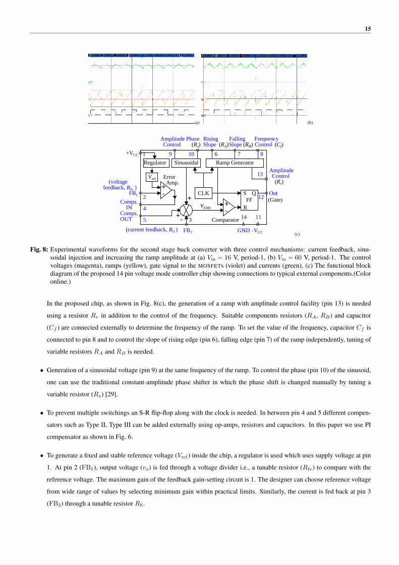
Fig. 8: Experimental waveforms for the second stage buck converter with three control mechanisms: current feedback, sinu-soidal injection and increasing the ramp amplitude at (a) Vin = 16 V, period-1, (b) Vin = 60 V, period-1. The controlvoltages (magenta), ramps (yellow), gate signal to the MOSFETs (violet) and currents (green), (c) The functional blockdiagram of the proposed 14 pin voltage mode controller chip showing connections to typical external components.(Coloronline.)

In the proposed chip, as shown in Fig. 8(c), the generation of a ramp with amplitude control facility (pin 13) is needed

using a resistor Rr in addition to the control of the frequency. Suitable components resistors (RA, RB) and capacitor

(Cf ) are connected externally to determine the frequency of the ramp. To set the value of the frequency, capacitor Cf is

connected to pin 8 and to control the slope of rising edge (pin 6), falling edge (pin 7) of the ramp independently, tuning of

variable resistors RA and RB is needed.

• Generation of a sinusoidal voltage (pin 9) at the same frequency of the ramp. To control the phase (pin 10) of the sinusoid,

one can use the traditional constant-amplitude phase shifter in which the phase shift is changed manually by tuning a

variable resistor (Rs) [29].

• To prevent multiple switchings an S-R flip-flop along with the clock is needed. In between pin 4 and 5 different compen-

sators such as Type II, Type III can be added externally using op-amps, resistors and capacitors. In this paper we use PI

compensator as shown in Fig. 6.

• To generate a fixed and stable reference voltage (Vref ) inside the chip, a regulator is used which uses supply voltage at pin

1. At pin 2 (FB1), output voltage (vo) is fed through a voltage divider i.e., a tunable resistor (Rfv) to compare with the

reference voltage. The maximum gain of the feedback gain-setting circuit is 1. The designer can choose reference voltage

from wide range of values by selecting minimum gain within practical limits. Similarly, the current is fed back at pin 3

(FB2) through a tunable resistor Rfi.

16

• The output signal of the compensator, current feedback signal, and sinusoidal signal are added to generate control signal

which is compared with the ramp. The output of the S-R flip-flop is available at pin 12 which drives the gate of the

MOSFET. The GND and negative supply −VCC of the chip are available at pin 14 and pin 11 respectively.

7 Conclusion

In this paper we have proposed the design guidelines of a controller chip that can drastically increase the operational parameter

ranges of power electronic systems, especially the complex converters like cascaded converters, resonant converters, and micro-

grids. The three techniques by which one can manipulate the terms that appear in the saltation matrices, can be integrated in a

single chip. These have been done in such a way that specific implementations will only need one to choose the external resis-

tances appropriately. This approach can control both fast-scale as well as slow-scale instabilities, without changing the intended

transient and steady-state performances. The idea has been experimentally validated using a system of cascaded buck converters,

by implementing the controller with discrete components. The basic purpose of this paper was to present a proof-of-concept on

the basis of which a chip development effort could be undertaken. The function of the proposed controller chip is the cumulative

effect of the functions of all the discrete components. The experimental results using discrete components show that the idea is

feasible. The fabrication and testing of such a chip are left for future work.

8 Acknowledgments

This project was funded by the National Plan for Science, Technology and Innovation (MAARIFAH) - King Abdulaziz City for

Science and Technology- the Kingdom of Saudi Arabia - award number (12-ENE3049-03). The authors also, acknowledge with

thanks Science and Technology Unit, King Abdulaziz University for technical support.

References

[1] Banerjee, S., Verghese, G. C.:‘Nonlinear Phenomena in Power Electronics — Attractors, Bifurcations, Chaos, and Non-

linear Control’ (IEEE Press, New York, 2001)

[2] Tse, C.K.: ‘Complex Behavior of Switching Power Converters’ (CRC Press, New York, 2003)

[3] El Aroudi, A., Giaouris, D., Iu, H.H.-C., Hiskens, I.: ‘A review on stability analysis methods for switching mode power

converters,’ IEEE Journal on Emerging Topics on Circuits and Systems, 2015, 5, (3), pp. 302–315

[4] Chakrabarty, K., Poddar, G., Banerjee, S.: ‘Bifurcation behavior of the buck converter,’ IEEE Transactions on Power

Electronics, 1996, 11, (3), pp. 439–447

[5] Fossas, E., Olivar, G.:‘Study of chaos in the buck converter,’ IEEE Transactions on Circuits and Systems-I, 1996, 43, (1),

pp. 12–25

[6] El Aroudi, A., Levya, R.: ‘Quasi-periodic route to chaos in a pwm voltage-controlled dc-dc boost converter,’ IEEE

Transactions on Circuits and Systems-I, 2001, 48, (8), pp. 967–978

17

[7] Zhou, G., Xu, J., Jin, Y.: ‘Elimination of subharmonic oscillation of digital-average-current-controlled switching dc-dc

converters,’ IEEE Transactions on Industrial Electronics, 2010, 57, (8), pp. 2904–2907

[8] Yu, D., Iu, H. H. C., Chen, H., Rodriguez, E., E. Alarcón, E., El Aroudi, A.: ‘Instabilities in digitally controlled

voltage-mode synchronous buck converter,’ International Journal on Bifurcation and Chaos, 2012, 22, (1), pp. 1 250 012–

1 250 012

[9] Singha, A.K., Kapat, S., Banerjee, S., Pal, J.: ‘Nonlinear analysis of discretization effects in a digital current mode

controlled boost converter,’ IEEE Journal on Emerging and selected Topics in Circuits and Systems, 2015, 5, (3), pp.

336–344

[10] Giaouris, D., Banerjee, S., Zahawi, B., Pickert, V.: ‘Stability analysis of the continuous conduction mode buck converter

via Filippov’s method,’ IEEE Transactions on Circuits Systems-I., 2008, 55, (4), pp. 1084–1096

[11] Giaouris, D., Maity, S., Banerjee, S., Pickert, V., Zahawi, B.: ‘Application of Filippov method for the analysis of sub-

harmonic instability in dc-dc converters,’ International Journal of Circuit Theory and Applications, 2009, 37, (8), pp.

899–919

[12] Zhou, Y., Tse, C.K., Qiu, S.S., Lau, F.C.M.: ‘Applying resonant parametric perturbation to control chaos in the buck dc/dc

converter with phase shift and frequency mismatch considerations,’ International Journal on Bifurcation and Chaos, 2003,

13, pp. 3459–3471

[13] Mandal, K., Abusorrah, A., Al-Hindawi, M.M., Al-Turki, Y., El Aroudi, A., Giaouris, D., Banerjee, S.: ‘Control-oriented

design guidelines to extend the Stability Margin of Switching Converters,’ IEEE International Symposium on Circuits

and Systems (ISCAS2017), 2017, accepted

[14] SGx524 Regulating Pulse-Width Modulators, Texas Instruments, SLVS077E, 2015

[15] TL494 Pulse-Width-Modulation Control Circuits, Texas Instruments, SLVS074G, 2015

[16] An, T.-J., Ahn, G.-C., Lee, S.-H.: ‘High-efficiency low-noise pulse-width modulation dcUdc buck converter based on

multi-partition switching for mobile system-on-a-chip applications,’ IEE IET Power Electronics, 2016, 9, (3), pp. 559–

567

[17] Chen, G., Hill, D. J., Yu, X.: ’Bifurcation Control: Theory and Applications’ (Springer-Verlag, New York, 2003).

[18] Leine, L.I., vanCampen, D.H.: ‘Discontinuous bifurcations of periodic solutions,’ Mathematical and Computer Modeling,

2002, 36, (3) pp. 259–273

[19] Cortés, J., Švikovic, V., Alou, P., Oliver, J.A., Cobos, J.A.: ‘v1 concept: Designing a voltage-mode control as current

mode with near time-optimal response for buck-type converters,’ IEEE Transactions on Power Electronics, 2015, 30, (10)

, pp. 5829–5841

[20] Rivetta, C.H., Emadi, A., Williamson, G.A., Jayabalan, R., Fahimi, B.: ‘Analysis and control of a buck dc-dc converter

operating with constant power load in sea and undersea vehicles,’ IEEE Transactions on Industry Applications, 2006, 42,

(2), pp. 559–572

18

[21] Vesti, S., Suntio, T., Oliver, J.A., Prieto, R., Cobos, J.A.: ‘Impedance-based stability and transient-performance assess-

ment applying maximum peak criteria,’ IEEE Transactions on Power Electronics, 2013, 28, (5), pp. 2099–2104

[22] Anshou, L., Donglai, Z.:‘Necessary and sufficient stability criterion and new forbidden region for load impedance speci-

fication,’ Chinese Journal of Electronics, 2014, 23, (3), pp. 1449–1453

[23] Riccobono, A., Santi, E.: ‘Comprehensive review of stability criteria for dc power distribution systems,’ IEEE Transac-

tions on Industry Applications, 2014, 50, (5), pp. 3525–3535

[24] Sanchez, S., Molinas, M.: ‘Assessment of a stability analysis tool for constant power loads in dc-grids,’ IEEE 15th

International Power Electronics and Motion Control Conference, 2012, pp. DS3b.2–1 – DS3b.2–5.

[25] Zhang, X., Ruan, X., Tse, C.K.: ‘Impedance-based local stability criterion for dc distributed power systems,’ IEEE

Transactions on Circuits and Systems–I, 2015, 62, (3), pp. 916–925

[26] Zadeh, M.K., Gavagsaz-Ghoachani, R., Martin, J.-P., Pierfederici, S., Nahid-Mobarakeh, B., Molinas, M.: ‘Discrete-time

tool for stability analysis of dc power electronics based cascaded systems,’ IEEE Transactions on Power Electronics,

2017, 32, (1). pp. 652–667

[27] Grigore, V., Hätönen, J., Kyyrä, J., Suntio, T.: ‘Dynamics of a buck converter with a constant power load,’ Proc. 29th

IEEE Power Electron. Spec. Conf., Fukuoka, Japan, May 1998, pp. 72–78

[28] Rahimi, A.M., Emadi, A.: ‘Discontinuous-conduction mode DC/DC converters feeding constant-power loads,’ IEEE

Transactions on Industrial Electronics, 2010, 57, (4), pp. 1318–1329

[29] Abuelma’atti, M.T., Baroudi, U.:‘A programmable phase shifter for sinusoidal signals,’ Active and Passive Electronic

Components, 1998, 21, (2), pp. 107–112