Dissertations and Theses

12-2017

Aviation Propulsive Lithium-Ion Battery Packs State-of-Charge and Aviation Propulsive Lithium-Ion Battery Packs State-of-Charge and

State-of-Health Estimations and Propulsive Battery System State-of-Health Estimations and Propulsive Battery System

Weight Analysis Weight Analysis

Jingsi Lilly

Follow this and additional works at: https://commons.erau.edu/edt

Part of the Aerospace Engineering Commons

Scholarly Commons Citation Scholarly Commons Citation Lilly, Jingsi, "Aviation Propulsive Lithium-Ion Battery Packs State-of-Charge and State-of-Health Estimations and Propulsive Battery System Weight Analysis" (2017). Dissertations and Theses. 367. https://commons.erau.edu/edt/367

This Thesis - Open Access is brought to you for free and open access by Scholarly Commons. It has been accepted for inclusion in Dissertations and Theses by an authorized administrator of Scholarly Commons. For more information, please contact commons@erau.edu.

AVIATION PROPULSIVE LITHIUM-ION BATTERY PACKS

STATE-OF-CHARGE AND STATE-OF-HEALTH ESTIMATIONS

AND PROPULSIVE BATTERY SYSTEM WEIGHT ANALYSIS

A Thesis

Submitted to the Faculty

of

Embry-Riddle Aeronautical University

by

Jingsi Lilly

In Partial Fulfillment of the

Requirements for the Degree

of

Master of Science in Aerospace Engineering

December 2017

Embry-Riddle Aeronautical University

Daytona Beach, Florida

iii

TABLE OF CONTENTS

Page

LIST OF TABLES . . . . . . . . . . . . . . . . . . . . . . . . . . . . . . . . v

LIST OF FIGURES . . . . . . . . . . . . . . . . . . . . . . . . . . . . . . . vi

SYMBOLS . . . . . . . . . . . . . . . . . . . . . . . . . . . . . . . . . . . . viii

ABBREVIATIONS . . . . . . . . . . . . . . . . . . . . . . . . . . . . . . . . x

ABSTRACT . . . . . . . . . . . . . . . . . . . . . . . . . . . . . . . . . . . xi

1 Introduction . . . . . . . . . . . . . . . . . . . . . . . . . . . . . . . . . . 11.1 Background . . . . . . . . . . . . . . . . . . . . . . . . . . . . . . . 11.2 Problem Statement . . . . . . . . . . . . . . . . . . . . . . . . . . . 41.3 HK-36 Electric Airplane . . . . . . . . . . . . . . . . . . . . . . . . 41.4 Propulsive Battery Systems . . . . . . . . . . . . . . . . . . . . . . 61.5 Battery Packs in Aviation Application . . . . . . . . . . . . . . . . 9

2 Literature Review . . . . . . . . . . . . . . . . . . . . . . . . . . . . . . . 112.1 Li-ion Single Cell Equivalent Circuit Model (ECM) . . . . . . . . . 112.2 SOC Estimation Methods . . . . . . . . . . . . . . . . . . . . . . . 14

2.2.1 Coulomb Counting Method . . . . . . . . . . . . . . . . . . 142.2.2 Open Circuit Voltage Method . . . . . . . . . . . . . . . . . 15

2.3 SOH Estimation Methods . . . . . . . . . . . . . . . . . . . . . . . 172.4 Battery Pack Modeling . . . . . . . . . . . . . . . . . . . . . . . . . 19

2.4.1 Cells Connected in Parallel . . . . . . . . . . . . . . . . . . . 192.4.2 Cells Connected in Series . . . . . . . . . . . . . . . . . . . . 20

2.5 Parameter Estimation . . . . . . . . . . . . . . . . . . . . . . . . . 212.5.1 Regular Least Squares . . . . . . . . . . . . . . . . . . . . . 212.5.2 Recursive Least Squares . . . . . . . . . . . . . . . . . . . . 24

3 Methodology . . . . . . . . . . . . . . . . . . . . . . . . . . . . . . . . . . 263.1 Li-ion Battery Equivalent Circuit Model (ECM) . . . . . . . . . . . 263.2 Recursive Least Squares (RLS) . . . . . . . . . . . . . . . . . . . . 283.3 SOC and SOH Estimations . . . . . . . . . . . . . . . . . . . . . . . 31

3.3.1 SOC Estimation . . . . . . . . . . . . . . . . . . . . . . . . . 323.3.2 SOH Estimation . . . . . . . . . . . . . . . . . . . . . . . . 323.3.3 Remaining Energy Estimation . . . . . . . . . . . . . . . . . 36

3.4 Pack Modeling . . . . . . . . . . . . . . . . . . . . . . . . . . . . . 383.5 Single Cell Simulation Model . . . . . . . . . . . . . . . . . . . . . . 40

iv

Page3.6 Weight Analysis . . . . . . . . . . . . . . . . . . . . . . . . . . . . . 42

4 Results and Analysis . . . . . . . . . . . . . . . . . . . . . . . . . . . . . 444.1 Single Cell Parameter Estimation . . . . . . . . . . . . . . . . . . . 444.2 Recursive Least Squares (RLS) Convergence . . . . . . . . . . . . . 55

4.2.1 RLS Based Estimation Algorithm . . . . . . . . . . . . . . . 554.2.2 System Excitation Analysis . . . . . . . . . . . . . . . . . . 574.2.3 RLS Validation Algorithm . . . . . . . . . . . . . . . . . . . 594.2.4 System Excitation Variance Study . . . . . . . . . . . . . . . 60

4.3 Example Case . . . . . . . . . . . . . . . . . . . . . . . . . . . . . . 654.4 HK-36 Battery System Weight Analysis . . . . . . . . . . . . . . . . 72

4.4.1 Li-ion Battery Cells Weight . . . . . . . . . . . . . . . . . . 724.4.2 Housing Structures Weight . . . . . . . . . . . . . . . . . . . 734.4.3 Cooling System Weight . . . . . . . . . . . . . . . . . . . . . 734.4.4 BMS Weight . . . . . . . . . . . . . . . . . . . . . . . . . . . 744.4.5 Wiring Weight . . . . . . . . . . . . . . . . . . . . . . . . . 744.4.6 Weight Fraction Results . . . . . . . . . . . . . . . . . . . . 75

5 Conclusion . . . . . . . . . . . . . . . . . . . . . . . . . . . . . . . . . . . 795.1 Significant Results . . . . . . . . . . . . . . . . . . . . . . . . . . . 795.2 Future Work . . . . . . . . . . . . . . . . . . . . . . . . . . . . . . . 80

REFERENCES . . . . . . . . . . . . . . . . . . . . . . . . . . . . . . . . . . 82

v

LIST OF TABLES

Table Page

1.1 Specifications of a NCR18650GA Cell . . . . . . . . . . . . . . . . . . . 7

2.1 Comparison of SOC Estimation Errors between the Thevenin model andthe DP model (He, Xiong, & Fan, 2011). . . . . . . . . . . . . . . . . . 13

4.1 Validation Results with “Forgetting Factor” λ Variations (at 1.6 BaseCurrent) . . . . . . . . . . . . . . . . . . . . . . . . . . . . . . . . . . . 61

4.2 Validation Results with “Forgetting Factor” λ Variations (at 8A Base Cur-rent) . . . . . . . . . . . . . . . . . . . . . . . . . . . . . . . . . . . . . 61

4.3 Validation Results with Amplitude Variations (at 1.6A Base Current) . 63

4.4 Validation Results with Amplitude Variations (at 8A Base Current) . . 63

4.5 Validation Results with Frequency Variations (at 1.6A Base Current) . 65

4.6 Validation Results with Frequency Variations (at 8A Base Current) . . 65

4.7 System Input Signal Key Items . . . . . . . . . . . . . . . . . . . . . . 66

4.8 Example Case Validation Results . . . . . . . . . . . . . . . . . . . . . 72

4.9 HK-36 Propulsive Battery Sub-systems Weight Fractions . . . . . . . . 76

4.10 HK-36 Propulsive Battery Sub-systems Weight Fractions with CapacityVariations . . . . . . . . . . . . . . . . . . . . . . . . . . . . . . . . . . 77

4.11 HK-36 Propulsive Battery Sub-systems Weight Fractions with Specific En-ergy Variations . . . . . . . . . . . . . . . . . . . . . . . . . . . . . . . 78

vi

LIST OF FIGURES

Figure Page

1.1 HK-36 Propulsive Battery Pack Configuration. . . . . . . . . . . . . . . 6

1.2 One Battery Module from the HK-36 Propulsive Battery Pack. . . . . . 6

1.3 Panasonic-Sanyo NCR18650GA Single Cell. . . . . . . . . . . . . . . . 7

2.1 Schematic Diagram of the Thevenin Equivalent Circuit Model (He et al.,2011). . . . . . . . . . . . . . . . . . . . . . . . . . . . . . . . . . . . . 12

2.2 Schematic Diagram of the DP Equivalent Circuit Model (He et al., 2011). 12

2.3 OCV-SOC Relations of Nine Batteries (Lee, Kim, Lee, & B.H.Cho, 2008). 16

2.4 OCV-SOC Relations under Different Temperatures (Huria, Ceraolo, Gaz-zarri, & Jackey, 2012). . . . . . . . . . . . . . . . . . . . . . . . . . . . 17

2.5 Simplify Serial Connected Cells into a Unit Model (Xiong, Sun, Gong, &He, 2013). . . . . . . . . . . . . . . . . . . . . . . . . . . . . . . . . . . 20

3.1 Schematic Diagram of the Thevenin Equivalent Circuit Model. . . . . . 26

3.2 RLS Iterative Process Algorithm. . . . . . . . . . . . . . . . . . . . . . 29

3.3 Capacity-Cycle Relation of a NCR18650GA Battery Cell (Panasonic, 2017). 34

3.4 Capacity-Cycle Relation of a NCR18650GA Battery Cell with ModifiedHorizontal Axis (Panasonic, 2017). . . . . . . . . . . . . . . . . . . . . 37

3.5 Example Battery Pack Configuration. . . . . . . . . . . . . . . . . . . . 39

3.6 Battery Packs Remaining Energy Estimation Algorithm. . . . . . . . . 39

3.7 Li-ion Single Cell Simulation Model. . . . . . . . . . . . . . . . . . . . 41

4.1 Single Cell Test Setup with the Vencon UBA5 Battery Analyzer & Charger. 44

4.2 Vencon UBA5 Battery Analyzer & Charger Testing Interface. . . . . . 45

4.3 Optimization Result at Iteration 0. . . . . . . . . . . . . . . . . . . . . 47

4.4 Optimization Result at Iteration 1. . . . . . . . . . . . . . . . . . . . . 48

4.5 Optimization Result at Iteration 15. . . . . . . . . . . . . . . . . . . . 49

4.6 Estimated Em vs. SOC Look-up-table. . . . . . . . . . . . . . . . . . . 50

vii

Figure Page

4.7 Estimated R0 vs. SOC Look-up-table. . . . . . . . . . . . . . . . . . . 50

4.8 Estimated R vs. SOC Look-up-table. . . . . . . . . . . . . . . . . . . . 51

4.9 Estimated C vs. SOC Look-up-table. . . . . . . . . . . . . . . . . . . . 51

4.10 Single Cell Simulation Model Validation Algorithm. . . . . . . . . . . . 52

4.11 Comparison between Experimental and Simulated Results at Constant3.3A Discharging. . . . . . . . . . . . . . . . . . . . . . . . . . . . . . . 53

4.12 Comparison between Experimental and Simulated Results at HK-36 FlightProfile discharging. . . . . . . . . . . . . . . . . . . . . . . . . . . . . . 54

4.13 RLS Based In-Flight SOC, SOH, and the Remaining Energy EstimationAlgorithm. . . . . . . . . . . . . . . . . . . . . . . . . . . . . . . . . . . 56

4.14 Example RLS System Input Signal with Sinusoidal Persistent Excitation. 58

4.15 RLS Validation Algorithm. . . . . . . . . . . . . . . . . . . . . . . . . . 59

4.16 Parameters with Abnormal Data After Converged. . . . . . . . . . . . 62

4.17 Li-ion Single Cell Simulation Model Setup. . . . . . . . . . . . . . . . . 67

4.18 Input Signal with Excitation of the Example Case. . . . . . . . . . . . 68

4.19 Error e(n) Convergence. . . . . . . . . . . . . . . . . . . . . . . . . . . 69

4.20 Zoomed In Error e(n) Convergence. . . . . . . . . . . . . . . . . . . . . 70

4.21 Estimated Parameters Convergence. . . . . . . . . . . . . . . . . . . . . 71

viii

SYMBOLS

b(n) System parameter vector at nth time step (expressed in recursiveleast squares)

C Capacitance of the capacitor in the RC parallel circuiteBat A battery cell’s available capacityeremain A battery cell’s remaining energye(n) Error at nth time stepEBat A battery pack’s available capacityEm Open circuit voltageEremain A cell unit’s remaining energyf(n) System excitations at nth time step (expressed in recursive least

squares)h(n) System excitation at nth time step (expressed in least squares)H System excitation matrix (expressed in least squares)I CurrentR Resistance of the resistor in the RC parallel circuitR0 Internal resistanceV Terminal voltageVRC Voltage across the RC parallel circuitW0 Aircraft maximum gross take-off weightWBat Propulsive battery system weightWBMS Battery management system weightWCell Propulsive battery cells weightWCool Battery pack cooling system weightWHouse Battery pack housing structures weightWWire Battery pack wiring system weightwBat Propulsive battery system weight fractionwBMS Battery management system weight fractionwCell Propulsive battery cells weight fractionwCool Battery pack cooling system weight fractionwHouse Battery pack housing structures weight fractionwWire Battery pack wiring system weight fractiontsignal Recursive least squares system input signal durationtconverge Recursive least squares converging timey(n) System measurements at nth time stepY System measurement matrixZ Battery impedance in generalZ0 Battery initial impedance

ix

Zact Battery actual impedanceZEOL Battery end-of-life impedanceεBat Battery specific energyεBat e Battery effective specific energyτRC Time constant of the RC parallel circuitθ(n) System parameters at nth time step (expressed in least squares)Θ System parameter matrix (expressed in least squares)

x

ABBREVIATIONS

AC Alternating currentAFM Airplane flight manualAWG American wire gaugeBMS Battery management systemCG Center of gravityDC Direct currentECM Equivalent circuit modelEFRC Eagle Flight Research CenterEIS Electrochemical impedance spectroscopyEKF Extended Kalman filterEOL End of lifeERAU Embry-Riddle Aeronautical UniversityEV Electric vehicleFAA Federal Aviation AdministrationPMPG Passenger miles per gallonGA General aviationLi-ion Lithium-ionMGTOW Maximum gross take-off weightNASA National Aeronautics and Space AdministrationOCV Open circuit voltagePCC Phase change compositeRLS Recursive least squaresRPM Revolutions per minuteSOC State-of-chargeSOH State-of-health

xi

ABSTRACT

Lilly, Jingsi MSAE, Embry-Riddle Aeronautical University, December 2017. Aviation

Propulsive Lithium-ion Battery Packs State-of-Charge and State-of-Health Estima-

tions And Propulsive Battery System Weight Analysis.

Aviation propulsive battery pack research is in high demand with the developmentof electric and hybrid aircraft. Accurate in-flight state-of-charge and state-of-healthestimations of aviation battery packs still remain challenging. This thesis puts effortson estimating the state-of-charge, state-of-health, and remaining energy of a lithium-ion propulsive battery pack with a recursive least squares based adaptive estimator.By reading the system measurements (discharging currents and terminal voltages)with persistent excitation, the proposed estimator can determine the present internalparameters of the battery cells and further interpolate them into state-of-charge,state-of-health, and the remaining energy information. The validation results indicatethat the recursive least squares based estimator achieves convergence within a veryshort time period (≈ 1 second) with desirable estimation accuracy (normally under1%).

To validate the recursive least squares based estimator, a lithium-ion single cellsimulation model is developed to simulate a NCR18650GA single cell’s performanceduring discharge at 25oC. Validations of the single cell simulation model with bothconstant discharging current and HK-36 flight mission profile show simulation errorsless than 1.3%.

This thesis also empirically analyzes the propulsive battery system weight andweight fractions based on the HK-36 electric airplane propulsive battery system de-signing experiences. As a result, the entire HK-36 propulsive battery system takesapproximately 27% of the aircraft gross weight. 58% of the battery system weightis the cells’ weight, and 42% is the auxiliary components weight. Taking the weightfraction into consideration, NCR18650GA cells’ effective specific energy reduces from0.16 HP-hr/lb (259 W-hr/kg) to 0.09 HP-hr/lb (150 W-hr/kg).

1

1. Introduction

1.1 Background

The aviation industry has been using fuel (such as 100LL and JetA) as the main

propulsive energy source since the 20th century. Traditional fuel-burning aviation en-

gines are accompanied by numerous environmental problems, such as green house gas

(CO2) emissions and noise pollution. Based on the published data from the U.S. En-

ergy Information Administration (EIA), aviation fuels (aviation gasoline and jet fuel)

account for approximately 12% of the total energy the U.S. transportation sector used

in 2016 (United States Energy Information Administration, 2017). The use of fuels

will keep increasing with the growth of the aviation industry. The Federal Aviation

Administration (FAA) forecasts that general aviation flying hours will increase an

average of 0.9% per year through 2037; meanwhile, operations at FAA and contract

towers are forecast to increase 0.8% a year for the next 20 years with commercial

activities growing at five times the rate of noncommercial activities (United States

Federal Aviation Administration, 2017).

To reduce the environmental impact that traditional aviation engines cause, al-

ternative aircraft propulsion solutions such as electric and hybrid aircraft have been

a popular research topic. As the core part of the propulsive system of electric and

hybrid aircraft, an electric motor uses electricity as an energy source instead of fuel.

2

Therefore, compared to conventional fuel-burning aviation engines, electric motors

have zero emissions during flight and are generally quieter at the same power setting.

The automotive industry is ahead of aviation in applying electricity as a source of

propulsion. Although similarities exist between the two industries, differences such

as operation temperature ranges, weight limitations, and safety requirements make it

necessary to study the aviation propulsive battery system design space separately.

Lithium-ion (Li-ion) batteries are frequently chosen as a propulsive electric source

by ground electric vehicles and electric/hybrid aircraft. This is because of lithium-

ion batteries’ relatively high gravimetric specific energy, high efficiency, long calender

and cycle lifetime, and low self-discharge (Stroe, Swierczynski, Kr, & Teodorescu,

2016). However, it should be noted that, although Li-ion batteries’ gravimetric spe-

cific energy is the highest among all available types of batteries, it is still much lower

than conventional aviation fuels (aviation gasoline and jet fuel). For example, the

NCR18650GA lithium-ion battery’s gravimetric specific energy is only 2.1% of AV-

GAS 100LL (Shell, 1999) (Panasonic, 2017); and only 2.2% of Jet A (kerosene) fuel

(Chevron Products Company, 2007).

Although Li-ion batteries have outstanding performance compared to most other

batteries, they should only be used within manufacturer specified limits. Inaccu-

rate state-of-charge and state-of-health estimations of Li-ion batteries can lead to

complications such as over-current, over-voltage, or under-voltage, which can com-

promise the battery performance, shorten battery life, or cause catastrophic safety

consequences.

3

The Eagle Flight Research Center (EFRC) under the Embry-Riddle Aeronauti-

cal University (ERAU) is one of the leading institutes of electric and hybrid aircraft

research. The EFRC has been researching both hybrid and fully electric airplanes

since 2011. One of its hybrid aircraft projects, Eco-Eagle, designed a parallel hybrid

aircraft to achieve the goal of flying 200 passenger miles per gallon (PMPG) of fuel

at an average speed of 100 miles per hour. It is designed to take-off using gasoline

and then switch to electric power at cruising conditions. This project has partici-

pated in the Green Flight Challenge which was sponsored by Google and hosted by

the National Aeronautics and Space Administration (NASA). Another project from

EFRC modifies a Diamond HK-36 motor glider into a fully electric airplane that uses

a lithium-ion battery pack to power a 100 HP electric motor. Its goal is to design and

build the first fully electric airplane certifiable by FAA in the United States. At the

same time, EFRC is also leading a hybrid electric research consortium that consists

of world-leading aviation companies and organizations to investigate specific hybrid

electric design tasks.

4

1.2 Problem Statement

The development of electric and hybrid airplanes has received increasing interest

from the aviation industry. Due to the nature of aircraft weight sensitivity, lithium-

ion batteries with high specific energy are frequently chosen as the propulsive energy

carriers for electric and hybrid airplanes. Use of lithium-ion batteries for propulsion

requires the development of a lightweight yet accurate in-flight energy estimation

method that takes into account the battery health degradation. This thesis proposes

an in-flight state-of-charge and state-of-health estimation algorithm that will serve as

a battery “fuel gauge”. It will adaptively estimate the instantaneous internal param-

eters of battery cells and further interpolate them to estimate the remaining energy of

the propulsive battery pack. To validate this algorithm, a lithium-ion cell simulation

model will be developed to simulate the cell behavior. Finally, the weight fraction of

propulsive battery systems will be analyzed empirically.

1.3 HK-36 Electric Airplane

The HK-36 electric airplane “e-Spirit of St. Louis” project (referred to by HK-

36 for the rest of the thesis) is one of the projects in Eagle Flight Research Center

(EFRC). The project’s goal is to modify the Diamond HK-36 motor glider into a fully

electric airplane and to certify it with the FAA. The HK-36 is a starting point of this

thesis. Some specific examples made in this thesis, as well as the weight analysis,

5

are based on the HK-36 propulsive battery system design. However, results and

conclusions from this research will be generic and may be applied to any configuration

of battery packs.

The original HK-36 airframe comes with a Rotax 914 engine to power a constant-

speed three-blade propeller. This engine delivers a maximum continuous power of

100HP (75kW) (Diamond Aircraft, 1997). The modified HK-36 electric airplane

replaces the Rotax engine with a YASA 750 axial flux electric motor that delivers

the same maximum continuous power of 100HP (75kW) (YASA Motors, 2017). The

original airplane stores its on-board energy source (100LL fuel) in a fuel tank; whereas

in the electric airplane, a propulsive battery pack takes place of the fuel tank and

carries the electricity energy to power the YASA motor.

The HK-36 propulsive battery pack contains a total of 2520 Li-ion cells. These

cells are electrically connected in parallel and series to meet the power requirements

of the motor. Figure 1.1 illustrates the configuration of the HK-36 propulsive battery

pack. In this figure, each red rectangle represents one battery cell. Seven cells are

connected in parallel to form a “cell unit.” This is the lowest observability for the

battery pack since only its combined current and terminal voltage can be observed

by the battery management system (BMS). Then, 12 “cell units” are connected in

series to form a “battery module”, which is represented by the black rectangles in the

diagram (also see Figure 1.2). Lastly, 30 of such “battery modules” are connected in

parallel and series to form the entire battery pack.

6

Figure 1.1 HK-36 Propulsive Battery Pack Configuration.

Figure 1.2 One Battery Module from the HK-36 Propulsive Battery Pack.

1.4 Propulsive Battery Systems

The most fundamental unit of a propulsive battery system is one single cell. The

type of Li-ion cells that HK-36 uses is NCR18650GA manufactured by Sanyo under

Panasonic (see Figure 1.3).

7

Figure 1.3 Panasonic-Sanyo NCR18650GA Single Cell.

“NCR” is a Panasonic short term for “Nickel/Cobalt/Rechargeable”, which refers

to the chemicals contained in the battery cells (Battery Bro, 2014). “18650” stands

for the standard cylindrical size of the cells: 18 mm diameter of cross-section and 65

mm of height. Table 1.1 summarizes some key specifications of the NCR18650GA

cells.

Table 1.1 Specifications of a NCR18650GA Cell

Items Values

Weight 48 g (0.106 lb)

Typical capacity at 25oC 3450 mAh

Nominal voltage 3.6 V

Based on these listed specifications, the NCR18650GA cells’ specific energy can

be calculated by Equation 1.1.

εBat =3.45Ah ∗ 3.6V

0.048kg= 259 W-hr/kg = 0.16 HP-hr/lb (1.1)

8

Although Li-ion batteries have relatively higher specific energy than other types

of batteries, the power and capacity that one single cell can deliver is limited and far

from sufficient to power an electric motor or to complete a flight. Therefore, cells are

usually connected in parallel, series, or a mixture of both to deliver desired power and

capacity. When assembling battery cells into a pack, other components are required

to assist the battery packs in delivering the electricity efficiently and safely. Battery

cells, together with other auxiliary components, form a propulsive battery system.

A typical propulsive battery system consists of five sub-systems:

• Battery cells: store electricity;

• Housing structures: secure cells and other components in place during move-

ment and vibration;

• Cooling system: passively or actively control the temperature of a battery pack;

• Battery management system (BMS): manage all of the cells within a battery

pack and protect them from operating outside of the manufacturer specified

limits;

• Wiring: electrically connect battery modules and deliver electricity to the mo-

tor.

9

1.5 Battery Packs in Aviation Application

An aviation propulsive battery system has numerous differences from a conven-

tional fuel-burning system. Pilots who are switching from a traditional airplane to

an electric airplane need to understand the differences before they take-off.

One of the differences a pilot might face first when preparing flight plans is that

the weight of a propulsive battery system does not change during flight, which means

that the landing weight remains almost the same as the take-off weight. In contrast,

the weight of a fuel-burning propulsion system gradually decreases when the engine

is consuming fuel.

Another difference is that the maximum power a battery pack can deliver will

decrease during flight. Maximum deliverable power is distributed by maximum al-

lowable current and terminal voltage from the pack. However, due to the nature of

Li-ion batteries, their terminal voltages gradually decrease during discharge. As a re-

sult, the maximum deliverable power will decrease. For example, one NCR18650GA

single cell’s maximum allowable current is 8A; its terminal voltage will decrease from

4.2V to 2.5V during discharge. At the beginning of discharge, the theoretical maxi-

mum power it can deliver is 8A x 4.2V, while at the end of discharge, its maximum

deliverable power reduces to 8A x 2.5V. Depending on the size (capacity) of a battery

pack, it might not be able to deliver the same take-off power again after the initial

take-off, even though the battery pack still has enough capacity left for cruising.

10

Moreover, unlike traditional fuel-burning airplanes whose fuel tank capacities re-

main constant, a Li-ion battery pack’s capacity declines after each flight cycle. This

is because of internal electrolyte loss of the battery cells during charging and dis-

charging.

Not only are there differences between traditional aviation fuel-burning propulsion

systems and propulsive Li-ion battery systems, but propulsive battery packs applied

in aviation industry also differ from the ones in ground electrical vehicles (EVs) in

the aspects of temperature range, safety, and weight.

Battery packs in electric airplanes operate in a wider temperature range than in

ground EVs. When parked or taxiing, electric airplanes deal with the same ground

temperatures as EVs. However, air temperatures at altitude are normally lower than

on the ground. Battery packs in cruising electric airplanes are therefore exposed to

lower ambient temperatures than in ground EVs.

Safety requirements of aviation battery packs are more restrictive than ground

EVs. In dangerous situations, ground vehicles may brake and stop in relatively shorter

time, while airplanes need comparatively longer time to descend and find open fields

to land. This results in higher safety expectations for aviation battery packs.

Due to airplanes’ sensitivity to weight and balance, aviation battery packs face

more critical weight limitations than ground EVs. As a result, all of the auxiliary

components inside of an aviation battery pack (such as BMS, wiring, cooling system,

etc.) need to be lightweight.

11

2. Literature Review

2.1 Li-ion Single Cell Equivalent Circuit Model (ECM)

The first step when analytically studying a Li-ion battery cell’s performance is to

look at its single cell equivalent circuit model (ECM). An ECM theoretically models

the chemical reaction inside of a battery cell as a nonlinear dynamical system that can

be mathematically described. More than one Li-ion ECMs were created by researchers

to fit different applications. In 2011, H.He et al. studied five types of commonly used

ECMs. The dynamic performances of the five ECMs were compared; furthermore,

the accuracies of their model-based state-of-charge (SOC) estimations were evaluated

(He et al., 2011).

Among the five ECMs studied and compared by this reference, two of them are

found to be more suitable in EV applications due to their better dynamic simulation

results. They are the Thevenin model and the DP model. Figures 2.1 and 2.2 show

the schematic diagrams of the two models individually.

12

Figure 2.1 Schematic Diagram of the Thevenin Equivalent CircuitModel (He et al., 2011).

Figure 2.2 Schematic Diagram of the DP Equivalent Circuit Model(He et al., 2011).

The Thevenin model and the DP model schematic diagrams have similar struc-

tures, both being composed of three major parts:

• Open circuit voltage UOC

• Ohmic resistance R0

• RC parallel circuit(s) with a set of resistors R and capacitors C in each circuit

13

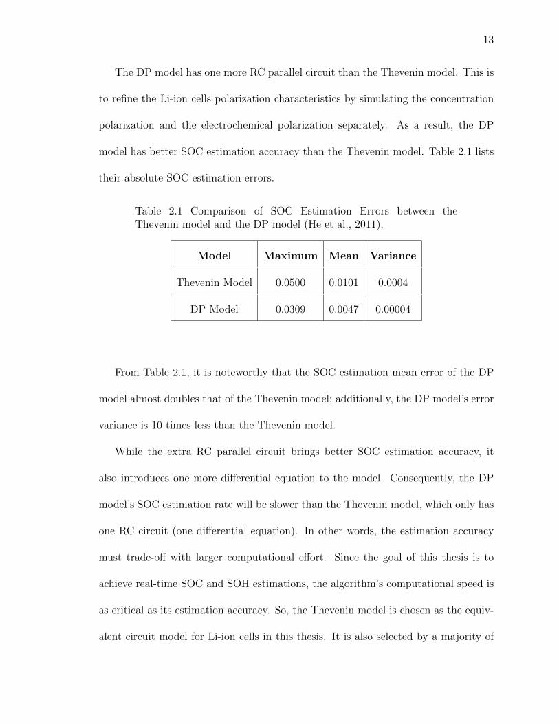
The DP model has one more RC parallel circuit than the Thevenin model. This is

to refine the Li-ion cells polarization characteristics by simulating the concentration

polarization and the electrochemical polarization separately. As a result, the DP

model has better SOC estimation accuracy than the Thevenin model. Table 2.1 lists

their absolute SOC estimation errors.

Table 2.1 Comparison of SOC Estimation Errors between theThevenin model and the DP model (He et al., 2011).

Model Maximum Mean Variance

Thevenin Model 0.0500 0.0101 0.0004

DP Model 0.0309 0.0047 0.00004

From Table 2.1, it is noteworthy that the SOC estimation mean error of the DP

model almost doubles that of the Thevenin model; additionally, the DP model’s error

variance is 10 times less than the Thevenin model.

While the extra RC parallel circuit brings better SOC estimation accuracy, it

also introduces one more differential equation to the model. Consequently, the DP

model’s SOC estimation rate will be slower than the Thevenin model, which only has

one RC circuit (one differential equation). In other words, the estimation accuracy

must trade-off with larger computational effort. Since the goal of this thesis is to

achieve real-time SOC and SOH estimations, the algorithm’s computational speed is

as critical as its estimation accuracy. So, the Thevenin model is chosen as the equiv-

alent circuit model for Li-ion cells in this thesis. It is also selected by a majority of

14

papers and articles for electric vehicles SOC and SOH estimation studies. However,

everything done in this thesis for the Thevenin-based models can be replicated using

DP models.

2.2 SOC Estimation Methods

Battery SOC is expressed in percentage to describe the energy left in a battery

with respect to its available capacity (after considering health degradation). For

example, a battery with 100% SOC is fully charged, while one with 0% SOC is

empty. In an electric airplane, it functions like a fuel gauge on a conventional fuel-

burning airplane. Unlike charging/discharging currents or terminal voltages, SOC is

not a physical property of batteries that can be directly measured. In most situations,

SOC is estimated by algorithms using other direct measurements.

Traditionally, two SOC estimation techniques are frequently used due to their

simplicity. They are the coulomb counting method and open circuit voltage method,

which will be introduced in the following two sub-sections.

2.2.1 Coulomb Counting Method

The Coulomb counting method is a rational way to estimate a battery’s SOC. In

this method, the current that is passing through the battery is monitored. Integrating

the measured current over time gives an estimated energy loss (Chaoui, Golbon,

15

Hmouz, Souissi, & Tahar, 2015). Therefore, SOC can be defined with Equation 2.1,

where EBat is the battery’s available capacity.

SOC =EBat −

∫Idt

EBat

(2.1)

The Coulomb counting method is simple, straightforward, and easily achieved

on-line. However, one of its main drawbacks besides startup errors, is that, due to

the integral, the measurement errors will accumulate over time, resulting in SOC

estimation drift.

2.2.2 Open Circuit Voltage Method

Another conventional SOC estimation technique is the open circuit voltage (OCV)

method. By definition, the open circuit voltage is the battery voltage under equilib-

rium conditions (Snihir, Rey, Verbitskiy, Belfadhel-Ayeb, & Notten, 2006). The OCV

method uses the correlation between OCV and electrolyte concentration that varies

with SOC. This correlation can be further represented by an OCV-SOC plot. This

plot is expected to remain the same during the life-time of the battery, i.e. it does not

depend on the age of the battery (Snihir et al., 2006). This makes OCV an excellent

indicator of SOC. But even for the same type of battery, different cells do not have

exactly the same OCV-SOC plots. However, they are close to each other with an

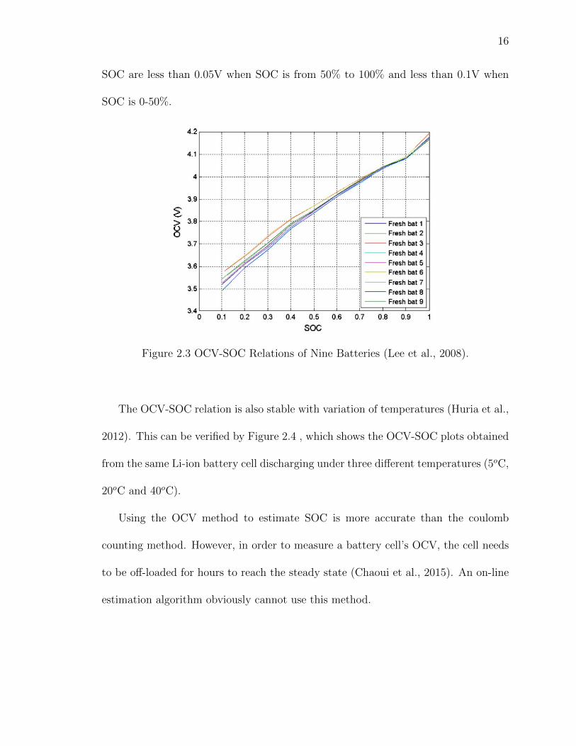
acceptable error. Figure 2.3 shows the OCV-SOC relationships of 9 fresh batteries

measured under the same conditions (Lee et al., 2008). From the figure, it can be

seen that the absolute maximum differences among the nine batteries at the same

16

SOC are less than 0.05V when SOC is from 50% to 100% and less than 0.1V when

SOC is 0-50%.

Figure 2.3 OCV-SOC Relations of Nine Batteries (Lee et al., 2008).

The OCV-SOC relation is also stable with variation of temperatures (Huria et al.,

2012). This can be verified by Figure 2.4 , which shows the OCV-SOC plots obtained

from the same Li-ion battery cell discharging under three different temperatures (5oC,

20oC and 40oC).

Using the OCV method to estimate SOC is more accurate than the coulomb

counting method. However, in order to measure a battery cell’s OCV, the cell needs

to be off-loaded for hours to reach the steady state (Chaoui et al., 2015). An on-line

estimation algorithm obviously cannot use this method.

17

Figure 2.4 OCV-SOC Relations under Different Temperatures (Huria et al., 2012).

In this thesis, the OCV method will be revised to estimate SOC. Instead of directly

measuring a battery’s OCV at steady state, an algorithm will be utilized to estimate

the OCV in real-time and further translate the OCV into SOC information.

2.3 SOH Estimation Methods

Li-ion batteries degrade as a result of their usage and exposure to environmental

conditions. This degradation affects the cells’ ability to store energy, meet power

demands and ultimately leads to their end-of-life (EOL) (Birkl, Roberts, McTurk,

Bruce, & Howey, 2017). Therefore, it is crucial for battery pack users to be certain

of the state-of-health (SOH) of the batteries to avoid misusing the battery packs.

Similar to SOC, SOH is also expressed as a percentage. Depending on the appli-

cations, there are usually two indicators of SOH – battery internal impedance and

18

capacity (Huang & Qahouq, 2014). Based on these two indicators, multiple SOH

estimation methods have been introduced.

One simple SOH estimation method uses the battery’s capacity as an indicator.

This method monitors the time needed for a fully charged battery to be completely

discharged by a small constant load. Utilizing the coulomb counting method, the total

energy loss can be calculated. The total energy loss is then equal to the battery’s

available capacity. However, it usually takes many hours to fully discharge a battery

and get its available capacity. Moreover, this method cannot be used during the

battery’s operation (Chaoui et al., 2015).

Another SOH estimation method regards the battery’s impedance as an indicator

by using electrochemical impedance spectroscopy (EIS). This method injects a small

sinusoidal voltage or current signal to an electrochemical cell, measuring the system’s

response with respect to amplitude and phase, determining the impedance of the

system by complex division of AC voltage by AC current, and repeating this for a

certain range of different frequencies (Karden, Buller, & Doncker, 2000). By analyzing

the impedance spectrum obtained from EIS, one can get the estimated impedance of a

battery. However, the EIS method requires additional hardware, costly measurement,

analysis instrumentation, and interruption of the system’s operation (Chaoui et al.,

2015).

Comparing the actual impedance of a battery with a reference impedance value

can be utilized as a measure of battery SOH as well. This reference impedance can

19

either be the impedance when the battery is new, or a value that is set based on

long-term experimental data (Huang & Qahouq, 2014).

This thesis proposes a hybrid approach that combines the methods mentioned

above to achieve on-line real-time SOH estimation.

2.4 Battery Pack Modeling

As discussed in the introductory chapter, multiple Li-ion cells need to be connected

into a pack to deliver the desired power and capacity. This raises the demand to

investigate battery pack modeling approaches. However, the majority of studies about

Li-ion battery SOC and SOH estimations focus on the single cell model. Only a few

of them discuss the pack model, such as the studies from Tripathy (2014) and Xiong

(2013).

2.4.1 Cells Connected in Parallel

Tripathy researches cases where Li-ion cells are connected in parallel (Tripathy,

McGordon, Marco, & Gama-Valdez, 2014). This research focuses on fault detection

among parallel connected cells. Although fault detection is not the focus of this thesis,

the article states that under normal operation, cells connected in parallel maintain

identical voltages, which results in the pack self-balancing to match terminal voltage

and SOC. This reference concludes that, if all cells are arranged in parallel, they can

20

be considered as a single “big” cell, with identical voltages and compounded capacities

(Tripathy et al., 2014).

This thesis uses this idea. In the HK-36 example, the minimum observability is

one “cell unit” – 7 cells connected in parallel – since no single cell within a cell unit

can be observed by the BMS. In order to estimate their SOC and SOH, such a “cell

unit” will be treated as a single “big” cell as Tripathy suggested in his paper.

2.4.2 Cells Connected in Series

In another article, Xiong analyzed the battery packs composed of Li-ion cells

connected in series (Xiong et al., 2013). Unlike cells connected in parallel where self-

balancing is done naturally, serial connected cells face the problem of capacity and

resistance unbalancing. To overcome the cell-to-cell variations problem, the authors

propose a cells filtering approach, where cells are pre-screened and only the ones with

similar capacities and resistances are selected to be connected in series. Following the

cells filtering process, the lumped parameter battery model with N cells is simplified as

a single cell model. Figure 2.5 illustrates how the serial connected cells are simplified

into a unit model.

Figure 2.5 Simplify Serial Connected Cells into a Unit Model (Xiong et al., 2013).

21

But, in most of the real world applications (including the HK-36 example), the

terminal voltage of each cell or “cell unit” in series is observed by the BMS. Thus

there is no need to simplify serial connected cells into a unit model.

2.5 Parameter Estimation

Parameter estimation functions as a mathematical tool that estimates the system

parameters by analyzing the system input or output information. Several common

parameter estimation methods are available and two of the most often used are in-

troduced in this section.

2.5.1 Regular Least Squares

Regular least squares estimation is one of the commonly chosen parameter esti-

mation approaches. Regular least squares assumes that the system measurements

(outputs) are corrupted with measurement errors, and the goal is to find a linear

combination of system parameters that gives the best fit to the noisy data (Gibbs,

2011). The system can be described by Equation 2.2 (Balas, 2017).

22

y = H ∗ θ + ε (2.2)

y – system measurements (outputs) vector

H – system excitation matrix

θ – system parameters vector

ε – system uncertainty (measurement error) vector

Expanding the vector terms, we get Equation 2.3 or Equation 2.4 (Balas, 2017).

y1

y2

· · ·

ym

=

[h1 h2 · · · hN

]

θ1

θ2

· · ·

θN

+ ε (2.3)

y = θ1h1 + θ2h2 + · · ·+ θNhN + ε (2.4)

When the system is described with a regression model, its estimated outputs at

nth time step can be expressed as Equation 2.5 (Balas, 2017).

y(n) =M∑i=1

θi(n− 1)h(n− 1) (2.5)

y(n) – estimated system measurements (outputs) vector at nth time step;

θ(n− 1) – unknown parameters vector at (n− 1)th time step;

h(n− 1) – system excitation at (n− 1)th time step.

23

The estimated parameters can then be calculated by taking the orthogonal projec-

tion of the system measurements (Balas, 2017). Equation 2.6 shows the least squares

estimator.

Θn−1 = (HTnHn)−1HnY n (2.6)

Note that Equation 2.5 describes the system in each time step. To distinguish

between Equations 2.5 and 2.6, Equation 2.6 uses capital letters for the three terms

(Θ, H and Y ). Each capital letter represents a matrix that contains information

from beginning to the current time step. For example, y(n) is the estimated system

measurement vector at nth time step, whereas Y n is a matrix containing vectors from

the beginning to the nth time step.

The regular least squares estimator works well in the cases where the system

measurements Y and excitation matrix H can be obtained all at once. On the con-

trary, in on-line estimation tasks, the system measurements and excitation matrices

can only be obtained sequentially from the sensors. Due to the high computational

cost, it is very inefficient to repeat Equation 2.6 at each time step to calculate the

parameters since the equation involves substantial matrix operations. Therefore, it

is essential to have a faster parameter estimation method for on-line estimation tasks.

24

2.5.2 Recursive Least Squares

To solve the mentioned problem that the regular least squares estimator has, this

section introduces an updated parameter estimation method – recursive least squares

(RLS). The forgetting factor λ term is introduced in RLS. λ (0 < λ ≤ 1) is an

exponential factor that is applied to each error term. Equations 2.7 and 2.8 compare

the error terms between regular least squares and RLS.

In regular least squares, the error ε is expressed as Equation 2.7.

ε(n) =n∑

i=0

e2(i) (2.7)

In RLS, the error is modified as Equation 2.8 (Rowell, 2008).

ε(n) =n∑

i=0

λn−ie2(i) (2.8)

The purpose of λ is to weigh recent data points most heavily, and thus track

changing statistics in the input data (Rowell, 2008). For example, in Equation 2.8,

when i = n (newest input data), the exponential term λn−i equals 1, and hence the

error term e2(n) is the most heavily weighed in the sum; conversely, when i = 0

(oldest input data), term λn−i equals λn ≤ 1, and therefore the error term e2(0) is

the most lightly weighed in the sum.

The advantage of RLS over regular least squares is that instead of re-estimating

the parameters using Equation 2.6 every time step when the system receives new input

data, RLS is able to apply an iterative algebraic procedure to update the parameters

using the results from previous time step, thus saving significant computational effort

(Rowell, 2008).

25

RLS has also been proven to be asymptotically stable and the parameters are expo-

nentially convergent provided that the system input is persistently exciting (Johnstone,

Johnson, Bitmead, & Anderson, 1982). Equation 2.9 shows the convergence of RLS

estimator error ε(n) (Balas, 2017).

||ε(n)|| ≤ K0λn||ε(0)|| (2.9)

26

3. Methodology

3.1 Li-ion Battery Equivalent Circuit Model (ECM)

Recall that in the literature review chapter, the Thevenin model is selected as

the Li-ion battery equivalent circuit model for this thesis. Figure 3.1 (modified from

Figure 2.1) illustrates the schematic diagram of Thevenin model.

Figure 3.1 Schematic Diagram of the Thevenin Equivalent Circuit Model.

The Thevenin Model consists of three parts:

• Open circuit voltage Em

• Ohmic resistance R0

• One RC parallel circuit with resistor R and capacitor C

27

In this model, the parameters of interest are Em, R0, R, and C. With these

four parameters, the system can be described by Equation set 3.1 with a first order

differential equation and a linear equation.VRC = − 1

RCVRC + 1

CI

V = Em − VRC −R0I

(3.1)

where:

I – Current

V – Terminal voltage

VRC – Voltage across RC parallel circuit

In order to estimate the parameters of interest, the first step is to transform

the system equations into a regression model. Equations 3.2 through 3.7 show the

transformation process:

Re-organize the second line in Equation set 3.1 to get VRC :

VRC = Em − V −R0I (3.2)

Take derivatives of both sides from Equation 3.2:

VRC = −R0I − V (3.3)

It is reasonable to assume that Em and R0 are slowly time-varying, so that Em ≈ 0

& R0 ≈ 0.

Next, substitute VRC and VRC back into the first line in Equation set 3.1:

−R0I − V = − 1

RC(Em −R0I − V ) +

1

CI (3.4)

28

Multiply both sides of Equation 3.4 by RC:

−RCR0I −RCV = −Em +R0I + V +RI (3.5)

Solve for V:

V = Em −RCV −RCR0I − (R +R0)I (3.6)

At last, the regression model of Thevenin Li-ion battery equivalent circuit model

can be recovered from Equation 3.6:

V =

[1 V I I

]

Em

−RC

−RCR0

−(R +R0)

(3.7)

3.2 Recursive Least Squares (RLS)

After obtaining the Li-ion single cell equivalent circuit model’s regression model,

the next step is to apply the RLS estimator to it. Equations 3.8 through 3.11 respec-

tively illustrate the y(n), f(n), and b(n − 1) with the corresponding terms from the

regression model.

y(n) = fT (n)b(n− 1) (3.8)

y(n) – system measurements (terminal voltage V (n)) at nth time step:

y(n) = V (n) (3.9)

29

fT (n) – system excitation vector (or RLS system input information) at nth time step:

fT (n) =

[1 V (n) I(n) I(n)

](3.10)

b(n− 1) – estimated parameters vector at (n− 1)th time step:

b(n− 1) =

Em(n− 1)

−R(n− 1)C(n− 1)

−R(n− 1)C(n− 1)R0(n− 1)

−[R(n− 1) +R0(n− 1)]

(3.11)

As discussed in the literature review chapter, RLS algorithm does not re-compute

Equation 2.6 at each time step; instead, it updates the estimated parameters with

an iterative algebraic process using information from the previous time step. The

iterative process is illustrated in the flow chart in Figure 3.2.

Figure 3.2 RLS Iterative Process Algorithm.

The iterative process can also be described mathematically by Equations 3.12

through 3.16 (Rowell, 2008).

30

Estimate the current system output with the system excitation from the current

time step and estimated parameter vector from the previous time step:

y(n) = fT (n)b(n− 1) (3.12)

Calculate the current error by comparing the current estimated system output

with the current measured output:

e(n) = y(n)− y(n) (3.13)

Update k(n):

k(n) =R−1(n− 1)f(n)

λ+ fT (n)R−1(n− 1)f(n)(3.14)

Update R−1(n):

R−1(n) = λ−1[R−1(n− 1)− k(n)fT (n)R−1(n− 1)] (3.15)

Update parameter vector b(n):

b(n) = b(n− 1) + k(n)e(n) (3.16)

Detailed derivations of the above equations and explanation about k(n) andR−1(n)

can be seen in MIT online course notes ”Introduction to Recursive-Least-Squares

(RLS) Adaptive Filters” written by D. Rowell (Rowell, 2008).

31

3.3 SOC and SOH Estimations

With an RLS estimator, the system parameters vector b(n) can be estimated

in real-time. However, b(n) does not explicitly give any SOC or SOH information.

This section proposes SOC and SOH estimation approaches using estimated b(n)

information.

The estimated parameter vector b(n) takes the form:

b(n) =

b1

b2

b3

b4

=

Em

−RC

−RCR0

−(R +R0)

(3.17)

Although Equation 3.17 does not directly give the four parameters of interest

individually (Em, R0, R, and C), they can be easily calculated from the four terms

in b(n). The results are shown in Equation set 3.18 below:

Em = b1

R0 = b3/b2

R = −b4 − b3/b2

C =b22

b2b4+b3

(3.18)

Once the four parameters of interest are calculated from b(n), the SOC and SOH

information can be estimated by the approaches in the next two sub-sections.

32

3.3.1 SOC Estimation

As mentioned in Section 2.2, this thesis revises the OCV method for SOC esti-

mation. Instead of directly measuring the OCV of a battery after waiting hours for

it to reach the steady state, the RLS algorithm allows OCV information (Em = b1)

to be estimated on-line in real-time. Thus, the SOC can be estimated through the

OCV-SOC look-up-table.

The OCV-SOC look-up-table will be obtained from the Design Optimization Tool

embedded in Simulink R©. The Design Optimization Tool is a parameter estimation

tool that fits the single cell simulation model (discussed in Section 3.5) to the battery

experimental data. Since it is just a tool that helps estimate parameters and collect

OCV-SOC look-up-tables, details of applying this tool can be seen in the article from

Huria (2012) and will not be reviewed in this thesis (Huria et al., 2012).

3.3.2 SOH Estimation

Section 2.3 reviewed literatures that study Li-ion battery SOH estimation meth-

ods. From those literatures, it can be found that both a battery’s capacity and

impedance (Z) can be used as indicators of SOH. This thesis uses a combination of

both indicators by assuming that both capacity and impedance have linear relations

with SOH. In other words, Z-SOH and SOH-Capacity relations can be described

by linear look-up-tables. First, by knowing a battery’s impedance Z, the Z-SOH

look-up-table is used to estimate SOH (discussed further in this section). Then, the

33

SOH-Capacity look-up-table is used to evaluate the actual capacity of a battery (dis-

cussed further in Section 3.3.3). SOH serves as an intermediate parameter to correlate

the estimated Z with capacity.

Before talking about a battery’s state-of-health (SOH), a definition of “health”

needs to be given. The battery industry usually uses a term called end-of-life (EOL),

which is a customizable threshold that denotes when the battery is not usable any-

more. Depending on different applications, EOL could be defined accordingly. For

example, one of the common definitions of EOL is “once the battery resistance

(impedance) increases to 160% of its initial value at the same condition” (Chaoui

et al., 2015) (Gholizadeh & Salmasi, 2014). In this thesis, the definition of EOL is

customized as follows:

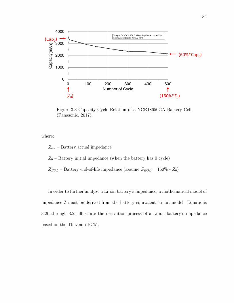
The capacity of a cell decreases to 60% of its initial capacity (about 500

cycles) at the same conditions (same temperature and same SOC); Mean-

while, the impedance of a cell increases to 160% of its initial impedance

at the same conditions.

Figure 3.3 visualizes the definition of EOL. This figure is modified from the

Capacity-Cycle plot obtained from the official datasheet of NCR18650GA cells from

Panasonic.

The SOH can then be expressed as a percentage and it is defined by the linear

Equation 3.19:

SOH =ZEOL − Zact

ZEOL − Z0

∗ 100% (3.19)

34

Figure 3.3 Capacity-Cycle Relation of a NCR18650GA Battery Cell(Panasonic, 2017).

where:

Zact – Battery actual impedance

Z0 – Battery initial impedance (when the battery has 0 cycle)

ZEOL – Battery end-of-life impedance (assume ZEOL = 160% ∗ Z0)

In order to further analyze a Li-ion battery’s impedance, a mathematical model of

impedance Z must be derived from the battery equivalent circuit model. Equations

3.20 through 3.25 illustrate the derivation process of a Li-ion battery’s impedance

based on the Thevenin ECM.

35

To start, a few assumptions need to be made to make the derivation process

possible:

• Current I is constant over each time step

• Initial time t0 = 0

• Initial voltage across the RC parallel circuit VRC(0) = 0

The derivation process starts with the system of equations, which is repeated in

Equation set 3.20: VRC = − 1

RCVRC + 1

CI

V = Em − VRC −R0I

(3.20)

Solve the first order differential equation in Equation set 3.20 for term VRC :

VRC = e−1

RCtVRC(0) +RI(1− e−

1RC

t) (3.21)

Since it is assumed that VRC(0) = 0, the first term in Equation 3.21 can be

dropped. Therefore, VRC can then be expressed as Equation 3.22

VRC = RI(1− e−1

RCt) (3.22)

Substitute Equation 3.22 back into the second line in Equation set 3.20 and write

out the terminal voltage V :

V = Em − [R(1− e−1

RCt) +R0] ∗ I (3.23)

The battery impedance can be extracted from Equation 3.23

Z =Em − V

I= R(1− e−

1RC

t) +R0 (3.24)

36

The equivalent impedance Z of a Li-ion single cell is:

Z = R(1− e−1

RCt) +R0 (3.25)

It can be seen that by Equation 3.25, a Li-ion single cell’s impedance Z can be

calculated with the R and R0 information estimated from RLS.

The impedance, Z, obtained here is the battery’s actual impedance, Zact. To get

its SOH, the initial impedance of a brand new battery Z0 is also needed. Conse-

quently, the initial R and R0 information is needed, which will also be obtained by

the Simulink R© Design Optimization Tool with experimental data from brand new

batteries.

3.3.3 Remaining Energy Estimation

SOC and SOH information is important for a battery. However, the ultimate goal

for a battery SOC and SOH estimation algorithm is to display a battery’s remaining

energy directly. In another words, instead of SOC and SOH values, a battery “fuel

gauge” is in demand for pilots.

The original chart in Figure 3.3 is obtained from the Panasonic NCR18650GA

official datasheet, which summarizes the experimental data showing how battery ca-

pacity changes after numbers of cycles. A cycle means that a battery experiences a

full charge followed by a full discharge. The data in the chart is only valid when the

battery is always charged and discharged with the same current profile as indicated

on the chart. However, users do not necessarily charge or discharge the battery packs

37

completely every time, nor do they use the same charge/discharge current as indicated

on the chart. This makes it difficult to keep track of or quantify the number of cycles

used. Therefore, the capacity-cycles relation in Figure 3.3 can not be directly applied

for capacity estimation. Instead, SOH can be used as an intermediate parameter to

correlate the impedance with capacity.

By assuming that SOH has a linear relation with number of cycles, the x-axis

(number of cycle) in Figure 3.4 can be replaced with SOH. Therefore, the Capacity-

Cycle chart can be transformed into a Capacity-SOH chart.

Figure 3.4 Capacity-Cycle Relation of a NCR18650GA Battery Cellwith Modified Horizontal Axis (Panasonic, 2017).

Section 3.3.2 has explained how to get SOH from the estimated parameters (R

and R0). Now with SOH, the battery’s actual capacity can be obtained through the

Capacity-SOH chart.

38

The battery’s remaining energy then can be expressed in Equation 3.26.

eremain = eBat ∗ SOC (3.26)

eremain – A battery cell’s remaining energy

eBat – A battery cell’s actual capacity

3.4 Pack Modeling

The SOC, SOH, and the remaining energy estimation algorithms previously dis-

cussed are all for a Li-ion single cell. However, in real cases, Li-ion cells are usually

assembled into a battery pack. Therefore, it is also important to study the SOC,

SOH, and the remaining energy estimation methods for battery pack applications.

Figure 3.5 illustrates an example battery pack model with two “cell units” con-

nected in series. Each cell unit contains n cells connected in parallel.

Usually, in a battery pack like this, the main-string current I and the terminal

voltages Vn are monitored by the BMS.

As discussed in Section 2.4.1, the n cells connected in parallel are assumed to

be identical. Therefore, each cell receives equivalently split current In. By inputing

the terminal voltage V and split current In

into the single cell RLS algorithm, the

remaining energy of a single cell can be estimated. Also, since the n cells connected

in parallel are identical, their compounded remaining energy Eremain will be n times

the single cell remaining energy eremain. This approach can be described by the flow

chart in Figure 3.6.

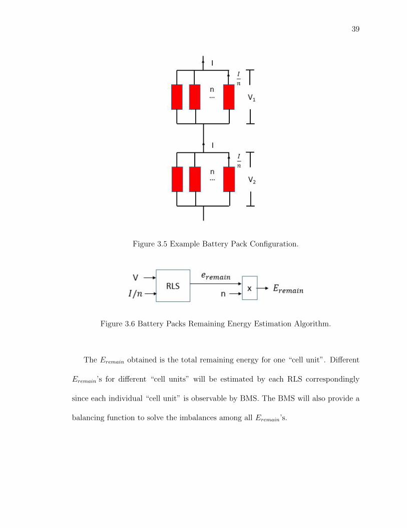
39

Figure 3.5 Example Battery Pack Configuration.

Figure 3.6 Battery Packs Remaining Energy Estimation Algorithm.

The Eremain obtained is the total remaining energy for one “cell unit”. Different

Eremain’s for different “cell units” will be estimated by each RLS correspondingly

since each individual “cell unit” is observable by BMS. The BMS will also provide a

balancing function to solve the imbalances among all Eremain’s.

40

3.5 Single Cell Simulation Model

In order to effectively validate the RLS algorithm’s estimation accuracy, experi-

mental data from real Li-ion battery cells being discharged under different conditions

must be obtained. However, extensive equipment and software are required to set up

experiments under different discharging conditions (such as different ambient temper-

atures and load currents). Additionally, it is very difficult to control or monitor the

internal parameters of a Li-ion cell during discharging. Moreover, it is time-consuming

to repeat the experiments since each charging and discharging cycle can take hours

to finish. Due to these difficulties, a Li-ion single cell simulation model that is able

to accurately simulate real cell performances is very beneficial.

One such model was developed by MathWorks R©, Inc. using the Simscape R© lan-

guage. The original model was designed to simulate multi-temperature Li-ion battery

performance with thermal dependence. This model essentially transforms a Thevenin

equivalent circuit model into a Simulink R© model. The internal parameter look-up-

tables in this model are estimated by the Simulink R© Design Optimization Tool using

pulse current discharge tests on high power lithium cells (LiNi-CoMnO2 cathode and

graphite-based anode) under different operating conditions. The model was validated

for a lithium cell with an independent drive cycle resulting in voltage accuracy within

2% (Huria et al., 2012).

This thesis, however, modifies the single cell simulation model to fit the needs of

this research. The major modification is that the internal parameter look-up-tables

41

in this model are estimated by the Design Optimization Tool using modified pulse

current discharge profiles on NCR18650GA Li-ion cells. The thermal effect is not

included in this model. All experimental data used for this modified model are eval-

uated at 25oC ambient temperature. Figure 3.7 shows the core of the modified single

cell simulation model.

Figure 3.7 Li-ion Single Cell Simulation Model.

42

3.6 Weight Analysis

In the aviation industry, weight and balance are two of the most sensitive design

factors, since nearly all of the aircraft performance has direct or indirect relation with

the aircraft gross weight.

The aircraft maximum gross take-off weight (MGTOW), W0, can be broken down

into the weight of each individual system that makes up the entire aircraft. Each

system can be further broken down into multiple sub-systems. To optimize each

system or sub-system’s performance while not compromising the aircraft MGTOW,

it is necessary to analyze the ratio of the weight of a certain sub-system to another

higher level system. Such a ratio is named as each system or sub-systems weight

fraction, w. For example, wBat represents the weight fraction of the battery system;

wMotor represents the weight fraction of the motor system, etc.

The propulsive battery system for electric airplanes functions as the fuel system

to the conventional fuel-burning aircraft. Its system weight, WBat, and corresponding

weight fraction, wBat, are of great interest to electric aircraft designers.

In the example of the HK-36 electric airplane, its propulsive battery system weight

consists of five parts: total weight of Li-ion cells WCell, weight of housing structures

WHouse, weight of its cooling system WCool, weight of the battery management system

WBMS, and weight of the harness wiring systemWWire. Equation 3.27 mathematically

describes the idea of their weight fractions.

wBat =WBat

W0

=WCell +WHouse +WCool +WBMS +WWire

W0

∗ 100% (3.27)

43

This thesis focuses on empirically analyzing the weight of a propulsive battery sys-

tem and its sub-systems as well as their weight fractions. All weight analysis will be

based on the propulsive battery system designing experiences from the HK-36 electric

airplane project. For each sub-system that makes up the HK-36 propulsive battery

system, two types of weight fractions will be studied: One is the weight fraction of

each sub-system in relation to the aircraft MGTOW, W0; the other is the weight

fraction of each sub-system in relation to the propulsive battery system total weight,

WBat. Finally, analysis of how specific energy variances and stored energy differences

affect the weight fractions of each sub-system within the propulsive battery system

will be performed.

44

4. Results and Analysis

4.1 Single Cell Parameter Estimation

The equipment used to collect NCR18650GA battery cells’ experimental test data

is the Vencon UBA5 Battery Analyzer & Charger. The UBA5 has two channels. Each

channel connects to the positive and negative terminals of one tested cell. At the same

time, the UBA5 is also connected to the computer with an RS232 cable. Figure 4.1

illustrates the experiments setup for single cell testings.

Figure 4.1 Single Cell Test Setup with the Vencon UBA5 BatteryAnalyzer & Charger.

45

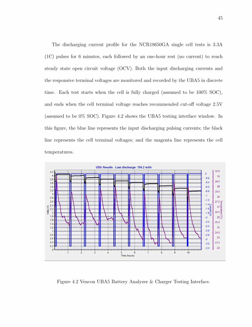
The discharging current profile for the NCR18650GA single cell tests is 3.3A

(1C) pulses for 6 minutes, each followed by an one-hour rest (no current) to reach

steady state open circuit voltage (OCV). Both the input discharging currents and

the responsive terminal voltages are monitored and recorded by the UBA5 in discrete

time. Each test starts when the cell is fully charged (assumed to be 100% SOC),

and ends when the cell terminal voltage reaches recommended cut-off voltage 2.5V

(assumed to be 0% SOC). Figure 4.2 shows the UBA5 testing interface window. In

this figure, the blue line represents the input discharging pulsing currents; the black

line represents the cell terminal voltages; and the magenta line represents the cell

temperatures.

Figure 4.2 Vencon UBA5 Battery Analyzer & Charger Testing Interface.

46

Besides the testing interface plots shown in Figure 4.2, the test results can also be

recorded into an excel datasheet. This enables the test results data to be imported

into the Design Optimization Tool to estimate the cell internal parameter look-up-

tables. The Design Optimization Tool then iteratively runs to optimize the parameter

look-up-tables in the single cell simulation model. The optimization iteration stops

when the relative sum of error squares between simulated and measured results is

changing by less than the set tolerance (1.0 ∗ 10−04).

Figures 4.3 through 4.5 show an example of the optimization process. In all three

figures, the top portion shows the terminal voltages (V) vs. time (s), and the bottom

portion shows the current (I) vs. time (s).

47

Figure 4.3 is the example when the optimization just starts (at iteration 0). The

red line (simulated terminal voltage) remains flat compared to the blue line (measured

terminal voltage). This is because the parameter look-up-tables that are in the single

cell simulation model are constants at this iteration (no variances at different SOC).

Figure 4.3 Optimization Result at Iteration 0.

48

Starting from iteration 1 (see Figure 4.4), the optimization tool has adjusted the

parameter look-up-tables, so the simulated results come closer to the measured results

compared to iteration 0.

Figure 4.4 Optimization Result at Iteration 1.

49

Depending on the test data, it might take the Design Optimization Tool different

numbers of iterations to finish the optimization. In the example shown, the optimiza-

tion stops at the 15th iteration (Figure 4.5).

Figure 4.5 Optimization Result at Iteration 15.

50

To minimize the estimation errors and cell variances, 8 different NCR18650GA

cells are tested. Averages of the parameter look-up-tables are used as the parame-

ters for the single cell simulation model. Figure 4.6 through 4.9 show the averaged

parameter look-up-tables.

0 0.1 0.2 0.3 0.4 0.5 0.6 0.7 0.8 0.9 1

State of Charge (%)

3

3.2

3.4

3.6

3.8

4

4.2

Em

(V

)

Average Em Look-up-table

Figure 4.6 Estimated Em vs. SOC Look-up-table.

0 0.1 0.2 0.3 0.4 0.5 0.6 0.7 0.8 0.9 1

State of Charge (%)

0.06

0.08

0.1

0.12

0.14

0.16

0.18

R0

Res

ista

nce

(Ω)

Average R0 Look-up-table

Figure 4.7 Estimated R0 vs. SOC Look-up-table.

51

0 0.1 0.2 0.3 0.4 0.5 0.6 0.7 0.8 0.9 1

State of Charge (%)

0

0.05

0.1

0.15

R R

esis

tanc

e (Ω

)

Average R Look-up-table

Figure 4.8 Estimated R vs. SOC Look-up-table.

0 0.1 0.2 0.3 0.4 0.5 0.6 0.7 0.8 0.9 1

State of Charge (%)

0

1

2

3

4

5

Cap

acita

nce

(F)

×104 Average C Look-up-table

Figure 4.9 Estimated C vs. SOC Look-up-table.

The next step is to validate the single cell simulation model with the averaged

parameter look-up-tables. The validation algorithm is described in Figure 4.10. First,

the same discharging current profiles are inputs for both the single cell simulation

model and the UBA5 battery analyzer. Then, their outputs (terminal voltages) from

the simulation model and the UBA5 are compared in order to obtain the absolute

and relative errors at each time step. Last, the average of the relative errors will be

regarded as the simulation model error.

52

Figure 4.10 Single Cell Simulation Model Validation Algorithm.

Two discharging current profiles are used to validate the single cell simulation

model:

• 3.3A (1C) constant discharging

• HK-36 flight profile: 8A constant discharging for 5 mins (simulating full-power

take-off current), followed by 1.6A constant discharging (simulating cruising

current)

The first validation results are plotted in Figure 4.11. The blue line shows the

experimental results, and the red line shows the simulated results. The yellow line

represents the absolute error between the experimental and estimated results. The

average relative error of this validation profile is evaluated at 1.24%.

53

0 500 1000 1500 2000 2500 3000 3500 4000

Time (s)

-0.5

0

0.5

1

1.5

2

2.5

3

3.5

4

4.5

Ter

min

al V

olta

ge (

V)

Comparison between Experimental and Simulated Results (Constant 3.3A Discharging)

Eperimental ResultsSimulated ResultsDelta

Figure 4.11 Comparison between Experimental and Simulated Resultsat Constant 3.3A Discharging.

The second validation results are plotted in Figure 4.12. Unlike the first constant

current discharging profile, the second profile pulls the maximum allowable current

from the cell first, then reduces the current to 20% of the take-off current until

the recommended cut-off voltage 2.5V is reached. The overall average relative error

of this validation profile is evaluated at 0.96%. Note that in this validation case,

the first discharging period (8A constant discharging) has relatively larger errors

compared to the second period (1.6A constant discharging). This may be caused by

the heat accumulation inside of the cell during 8A discharging. When Li-ion cells are

discharged at a higher current, the cell’s internal impedance (or resistance) will cause

the cells to generate comparatively more heat than that discharged at a lower current.

The experimental results from UBA5 recorded that the cell temperature increased to

54

40oC while being discharged at 8A current. However, this single cell simulation model

parameter look-up-tables are estimated at 25oC. Therefore, it is expected that the

simulation accuracy decreases at 8A discharging.

0 1000 2000 3000 4000 5000 6000 7000

Time (s)

-0.5

0

0.5

1

1.5

2

2.5

3

3.5

4

4.5

Ter

min

al V

olta

ge (

V)

Comparison between Experimental and Simulated Results (HK36 Flight Profile)

Eperimental ResultsSimulated ResultsDelta

Figure 4.12 Comparison between Experimental and Simulated Resultsat HK-36 Flight Profile discharging.

From the two validation results, it can be seen that the average relative errors

under two different discharging profiles are both below 1.5%. It can be concluded

that the single cell simulation model is valid to simulate the NCR18650GA single

cell behavior while being discharged at 25oC. The model then can be used to collect

the system excitation information for RLS estimator and further validate the RLS

based in-flight SOC and SOH estimation algorithm. However, the simulation model

has some limitations. The modified model does not include any cell internal ther-

mal behavior, nor does it consider the heat exchange with the ambient environment.

55

Additionally, the parameter look-up-tables are only estimated for discharging con-

dition. Therefore, the single cell simulation model is only valid to simulate the cell

discharging behavior at 25oC ambient temperature.

Although the above limitations exist in this simulation model, they can be over-

come by repeating the same parameter estimation process using the Design Opti-

mization Tool with experimental data under other test conditions. Similarly, the

model can be further modified to fit other types of Li-ion batteries except for the

NCR18650GA cells.

4.2 Recursive Least Squares (RLS) Convergence

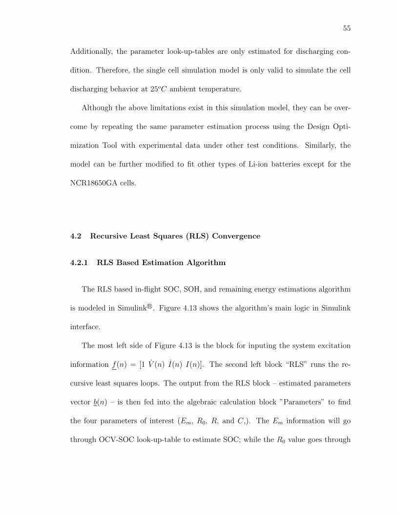
4.2.1 RLS Based Estimation Algorithm

The RLS based in-flight SOC, SOH, and remaining energy estimations algorithm

is modeled in Simulink R©. Figure 4.13 shows the algorithm’s main logic in Simulink

interface.

The most left side of Figure 4.13 is the block for inputing the system excitation

information f(n) = [1 V (n) I(n) I(n)]. The second left block “RLS” runs the re-

cursive least squares loops. The output from the RLS block – estimated parameters

vector b(n) – is then fed into the algebraic calculation block ”Parameters” to find

the four parameters of interest (Em, R0, R, and C,). The Em information will go

through OCV-SOC look-up-table to estimate SOC; while the R0 value goes through

56

Figure 4.13 RLS Based In-Flight SOC, SOH, and the Remaining En-ergy Estimation Algorithm.

Z-SOH look-up-table to estimated the actual capacity of the cell. By multiplying the

estimated SOC with the cell’s actual capacity, the energy left inside of a cell at that

moment can be evaluated.

According to the impedance (Z) equation (repeated in Equation 4.1), both R0 and

R values are needed to calculate the cell impedance.

Z = R(1− e−1

RCt) +R0 (4.1)

However, it can be seen in Figure 4.13 that only the R0 information is routed into

the Z-SOH look-up-table.

From the single cell parameter estimation results, the averaged values of R and C

are found to be:

Ravg = 0.045 Ω; Cavg = 18932 F (4.2)

57

The time constant for the RC parallel circuit then can be calculated in Equation

4.3:

τRC = RavgCavg = 852 seconds (4.3)

Comparatively, the RLS algorithm system excitation signal duration tsignal lasts

about 5 seconds, which is far less than the time constant of the dynamic RC circuit

τRC . From Equation 4.1, it can be seen that when time t is a small value, the entire

R(1− e− 1RC

t) term is close to 0. Therefore, it can be asssumed that when the system

input signal duration tsignal is small, the cell impedance Z can be approximated to

be R0 (see Equation 4.4).

Z ≈ R0 (tsignal << τ) (4.4)

4.2.2 System Excitation Analysis

Recall from Section 2.5.2 that RLS is asymptotically stable and its estimation

results are convergent only when the systems are persistently excited (Johnstone et

al., 1982). In the example of this thesis, it means that the RLS system input signal

f(n) = [1 V (n) I(n) I(n)] must have persistent excitation.

Square waves/pulses that are similar to the ones used in the single cell simulation

model parameter estimation experiments are considered first. However, this type of

excitation fails because of the derivative terms in the system input vector (V and I).

If square waves/pulses are used, the derivatives of pulsing edges will be infinity and

cause singularities, therefore they cannot be used as RLS system excitation signals.

58

Sinusoidal signals are better options in this case. With sine waves, all terms in

the RLS input signal vector can be measured or calculated easily in discrete time

without singularities. Additionally, adding a relatively small sinusoidal current into

the base discharging current brings comparatively low disruption impact to the system

operation compared to pulsing signals.

Figure 4.14 shows an example of RLS system input signal with sinusoidal persis-

tent excitation.

0 50 100 150 200 250 300 350 400 450 5000

1

2

One

Input Signal

0 50 100 150 200 250 300 350 400 450 500-0.2

0

0.2

Vd

ot

0 50 100 150 200 250 300 350 400 450 500-2

0

2

I do

t

0 50 100 150 200 250 300 350 400 450 500

Time Steps

1

1.5

2

I(A

)

Figure 4.14 Example RLS System Input Signal with Sinusoidal Per-sistent Excitation.

59

4.2.3 RLS Validation Algorithm

Before studying how the system excitation variances affect the RLS estimation

accuracy in next section, the RLS validation algorithm must be discussed. Figure

4.15 illustrates the RLS validation logic in a flow chart.

Figure 4.15 RLS Validation Algorithm.

The discharging current profile to be validated is setup as the input of the sin-

gle cell simulation model. Running a simulation of the model gives the responding

terminal voltages. After obtaining the currents and terminal voltages information in

discrete time, the derivative terms (V and I) can be calculated and the RLS system

input signal f can be formed. Inputting the system excitation f into RLS is the

next step. The RLS estimator then estimates the present status of the simulated cell

60

(including the four internal parameters, SOC, SOH, and remaining energy). Once

completed with all previous steps, compare all of the estimated parameters obtained

from RLS with the setup parameters in the simulation model and calculate corre-

sponding errors of each parameter.

4.2.4 System Excitation Variance Study

Using the RLS validation algorithm, different system excitations can be sent into

the RLS estimator and the estimation accuracies under different inputs can be vali-

dated.

In this section, three system excitation variances are of interest:

• Forgetting factor λ variances

• System excitation amplitude variances

• System excitation frequency variances

The forgetting factor λ variations are studied first. Tables 4.1 and 4.2 compare five

validation cases where only λ is varied. All validation cases in Table 4.1 have a base

discharging current of 1.6A (HK-36 cruising condition), and the sinusoidal excitation

amplitude is 0.2A while Table 4.2 contains validation cases with a base discharging

current of 8A (HK-36 take-off condition) and the sinusoidal excitation amplitude

is 1A. The converging time tconverge is defined as when the error e(n) stays within

±0.001. All ten cases have the same excitation frequency of 1Hz. The simulated cell

is set to be at 50% SOC.

61

Table 4.1 Validation Results with “Forgetting Factor” λ Variations(at 1.6 Base Current)

No. λ tconverg(s) SOC Error (%) Z Error (%)

1 0.99 3.0 0.06 0.01

2 0.95 0.9 0.12 0.01

3 0.93 0.8 0.12 0.01

4 0.9 0.7 0.14 0.01

5 0.8 0.4 0.14 0.01

Table 4.2 Validation Results with “Forgetting Factor” λ Variations(at 8A Base Current)

No. λ tconverg (s) SOC Error (%) Z Error (%)

1 0.99 >5 1.83 0.02

2 0.95 0.9 1.94 0.02

3 0.93 0.8 0.40 0.02

4 0.9 0.7 1.13 0.04

5 0.8 0.4 0.56 0.02

From the validation cases in Tables 4.1 and 4.2, it can be seen that λ has a

direct impact on the system convergence rate. The smaller λ is, the faster the system

converges. At the same time, λ causes small changes in the SOC and impedance

62

estimation accuracies. However, the changes do not show an obvious trend with an

optimizing λ that gives the best SOC and impedance accuracies.

It needs to be pointed out that even though it is ideal to have a faster converging

rate for the estimation algorithm, there is a threshold of λ after which the estimation

is not valid. The turning point varies depending on different system input excitation

signals. For the cases validated in Tables 4.1 and 4.2, the turning point happens

around λ = 0.9. When λ < 0.9, the parameters plots show abnormal data after con-

verging (see Figure 4.16 as an example). To avoid this abnormal data, λ cannot be set

to be smaller than this threshold (0.9). Additionally, for the validation cases where

converging time is less than one second, both Tables 4.1 and 4.2 show an minimum

SOC and impedance error at λ = 0.93.

Figure 4.16 Parameters with Abnormal Data After Converged.

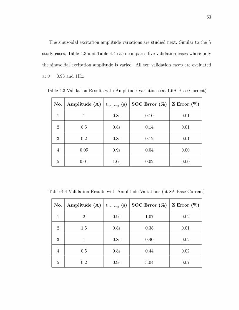
63

The sinusoidal excitation amplitude variations are studied next. Similar to the λ

study cases, Table 4.3 and Table 4.4 each compares five validation cases where only

the sinusoidal excitation amplitude is varied. All ten validation cases are evaluated

at λ = 0.93 and 1Hz.

Table 4.3 Validation Results with Amplitude Variations (at 1.6A Base Current)

No. Amplitude (A) tconverg (s) SOC Error (%) Z Error (%)

1 1 0.8s 0.10 0.01

2 0.5 0.8s 0.14 0.01

3 0.2 0.8s 0.12 0.01

4 0.05 0.9s 0.04 0.00

5 0.01 1.0s 0.02 0.00

Table 4.4 Validation Results with Amplitude Variations (at 8A Base Current)

No. Amplitude (A) tconverg (s) SOC Error (%) Z Error (%)

1 2 0.9s 1.07 0.02

2 1.5 0.8s 0.38 0.01

3 1 0.8s 0.40 0.02

4 0.5 0.8s 0.44 0.02

5 0.2 0.9s 3.04 0.07

64

By comparing Tables 4.3 and 4.4, it can be found that for different base discharg-

ing currents, the required excitation amplitudes to achieve convergence are different.

Generally speaking, larger base currents require relatively larger excitation ampli-

tudes. In both tables, amplitude variances can be found to cause slight changes in

convergence rate, SOC error, and impedance error. In 1.6A base current cases, an

amplitude of 0.01A gives the best SOC and impedance estimation accuracies at the

cost of relatively longer converging time. In 8A base current cases, however, an am-

plitude of 1.5A results in the best convergence rate, as well as SOC and impedance

estimation accuracies. However, it should be noted that the amplitudes with the best

estimation accuracies are not necessary in many situations. Smaller amplitudes with

acceptable estimation errors and convergence rates can also be applied in order to

minimize the interruption of system operation.

The sinusoidal excitation frequency variations are also studied. Table 4.5 com-

pares six validation cases where only the sinusoidal excitation frequency is varied.

Their base discharging currents are 1.6A, and their excitation amplitudes are 0.05A.

Similarly, Table 4.6 compares four frequencies with a base discharging current of 8A

and an excitation of 1A. All ten validation cases are evaluated at λ = 0.93.

From both Tables 4.5 and 4.6, it can be seen that 1Hz works the best for both

1.6A and 8A base current cases. However, lower frequencies with acceptable estima-

tion errors and convergence rates can also be applied if minimum system operation

interruption is desired.

65

Table 4.5 Validation Results with Frequency Variations (at 1.6A Base Current)

No. Frequency (Hz) tconverge (s) SOC Error (%) Z Error (%)

1 5 0.8s 0.75% 0.02%

2 2 0.9s 0.30% 0.01%

3 1 0.9s 0.04% 0.00%

4 0.5 1.2s 0.32% 0.01%

5 0.1 0.4s 0.53% 0.14%

6 0.05 0.4s 5.01% 0.37%

Table 4.6 Validation Results with Frequency Variations (at 8A Base Current)

No. Frequency (Hz) tconverge (s) SOC Error (%) Z Error (%)

1 5 2.8 4.62% 0.07%

2 2 0.6 0.56% 0.01%

3 1 0.8 0.40% 0.02%

4 0.5 1.0s 4.01% 0.02%

4.3 Example Case

In order to demonstrate how the SOC, SOH, and the remaining energy estimation

algorithms work on a Li-ion cell, detailed step-by-step procedures will be shown in

this section.

66

The discharging profiles with system excitations must be determined first. In this

example, 1.6A base discharging current will be used to show how the estimation algo-

rithm works using the HK-36 electric airplane cruising flight condition. A sinusoidal

excitation with 0.05A amplitude and 1Hz frequency will be added on top of the base

discharging current. The system input items are listed in Table 4.7.

Table 4.7 System Input Signal Key Items

Item Value

Base Current -1.6A

Amplitude 0.05A

Frequency 1Hz (3.14 rad/s)

Input Signal Duration 5 seconds

Step Size 0.01s (500 steps total)

SOC 50.66%

Forgetting Factor λ 0.95

All of the key items will be set up in the Li-ion single cell simulation model to get

the simulated terminal voltages based on the input discharging current profile. See

Figure 4.17 for simulation model set up.

67

Figure 4.17 Li-ion Single Cell Simulation Model Setup.

The single cell simulation model with the setup values in Table 4.7 will produce the

simulated cell terminal voltages. With the currents and terminal voltages in discrete

time, the derivative terms V and I in RLS system input vectors f can be approxi-

mately calculated. The pre-determined RLS input vectors can then be concatenated

into a full matrix. Figure 4.18 shows the full length of the pre-determined input signal

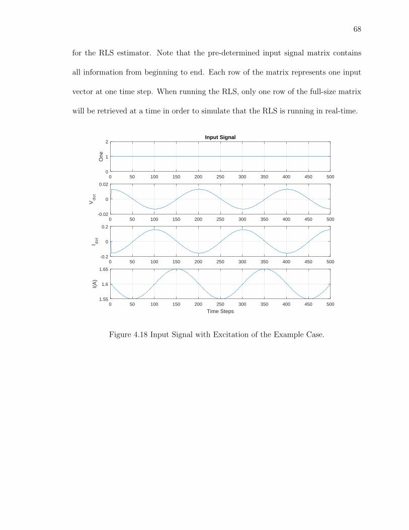
68

for the RLS estimator. Note that the pre-determined input signal matrix contains

all information from beginning to end. Each row of the matrix represents one input

vector at one time step. When running the RLS, only one row of the full-size matrix

will be retrieved at a time in order to simulate that the RLS is running in real-time.

0 50 100 150 200 250 300 350 400 450 5000

1

2

One

Input Signal

0 50 100 150 200 250 300 350 400 450 500-0.02

0

0.02

Vd

ot

0 50 100 150 200 250 300 350 400 450 500-0.2

0

0.2

I do

t

0 50 100 150 200 250 300 350 400 450 500

Time Steps

1.55

1.6

1.65

I(A

)

Figure 4.18 Input Signal with Excitation of the Example Case.

69

Figure 4.19 shows the error e(n) convergence along the time steps. Earlier in

this section, the convergence of e(n) is defined when e(n) stays within 0.001. Zoom-

ing in the e(n) plot (see Figure 4.20), it can be seen that the error converges after

approximately 1.5 seconds (150 time steps).

0 50 100 150 200 250 300 350 400 450 500

Time Steps

-0.15

-0.1

-0.05

0

0.05

0.1

0.15

e (V

olts

)

Error e(n)

Figure 4.19 Error e(n) Convergence.

70

0 50 100 150 200 250 300 350 400 450 500

Time Steps

-3

-2

-1

0

1

2

3

4

5

6

e (V

olts

)

×10-3 Error e(n)

X: 144Y: 0.001031

Figure 4.20 Zoomed In Error e(n) Convergence.

Figure 4.21 shows the estimated parameters’ convergence. Similar to the error

e(n) convergence, all four parameters achieve convergence after about 1.5 seconds

(150 time steps).

71

0 50 100 150 200 250 300 350 400 450 5003.5

3.6

3.7

3.8

3.9

Em

(V)

Estimated Parameters

0 50 100 150 200 250 300 350 400 450 5000.08

0.082

0.084

R0(Ω

)

0 50 100 150 200 250 300 350 400 450 5000

0.05

0.1

R(Ω

)

0 50 100 150 200 250 300 350 400 450 500

Time Steps

0

2

4

6

C(F

)

×104

Figure 4.21 Estimated Parameters Convergence.

The validation results of this example case are listed in Table 4.8. The results

show very good estimation accuracies. The SOC and impedance accuracies are under

0.1%, while the available capacity and remaining energy accuracies are around 1%.

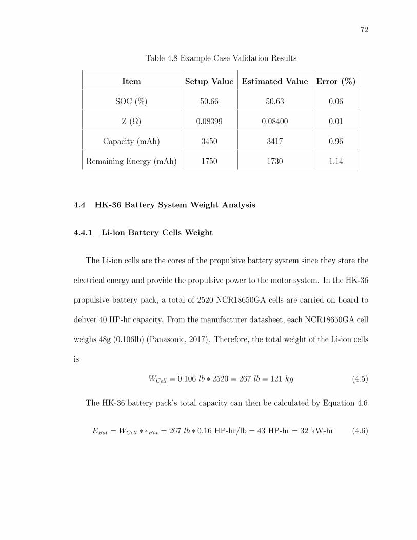
72

Table 4.8 Example Case Validation Results

Item Setup Value Estimated Value Error (%)

SOC (%) 50.66 50.63 0.06

Z (Ω) 0.08399 0.08400 0.01

Capacity (mAh) 3450 3417 0.96

Remaining Energy (mAh) 1750 1730 1.14

4.4 HK-36 Battery System Weight Analysis

4.4.1 Li-ion Battery Cells Weight

The Li-ion cells are the cores of the propulsive battery system since they store the

electrical energy and provide the propulsive power to the motor system. In the HK-36

propulsive battery pack, a total of 2520 NCR18650GA cells are carried on board to

deliver 40 HP-hr capacity. From the manufacturer datasheet, each NCR18650GA cell

weighs 48g (0.106lb) (Panasonic, 2017). Therefore, the total weight of the Li-ion cells

is

WCell = 0.106 lb ∗ 2520 = 267 lb = 121 kg (4.5)

The HK-36 battery pack’s total capacity can then be calculated by Equation 4.6

EBat = WCell ∗ εBat = 267 lb ∗ 0.16 HP-hr/lb = 43 HP-hr = 32 kW-hr (4.6)

73

4.4.2 Housing Structures Weight

The HK-36 battery pack uses a translucent amber material called Ultem as the

top and bottom covers of each battery module. The Ultem material in each battery

module weighs 0.4 kg (0.88 lb). All of the other auxiliary structural components (such

as straps and screws) for the entire 30 battery modules weigh approximately 0.5 kg

(1.1 lb). Therefore, the total weight of housing structures in the battery pack can be

calculated by Equation 4.7:

WHouse = 0.88 lb ∗ 30 + 1.1 lb = 28 lb = 13 kg (4.7)

4.4.3 Cooling System Weight

The HK-36 electric airplane has a passive air-cooling system. The cooling system

is composed of three parts: Phase Change Composite (PCC), cooling fins, and air

ducts. The PCC material is a special graphite that absorbs the heat generated by the

battery cells to prevent heat propagation among them. Cooling fins are aluminum

fins or plates that transfer heat from PCC to the air flow. Air ducts are used to

route the air flow that circulates around the battery modules to transfer the heat

from cooling fins and BMS to external outlets.

Each battery module has one PCC brick, which weighs 0.7 kg (1.6 lb). The cooling

fins, together with air ducts, weigh 7.5 kg (16.6 lb). Therefore, the HK-36 battery

pack cooling system total weight is

WCool = 1.6 lb ∗ 30 + 16.6 lb = 63 lb = 29 kg (4.8)

74

4.4.4 BMS Weight

The BMS of HK-36 consists of all of the PCB boards that provide connectivity

and management among cells within a battery module. Each battery module has

three PCBs. The three PCBs, together with their mounted electric components and

battery contact leaf springs, weigh 0.9 kg (2.0 lb) in total. Therefore, the total BMS

weight of the entire battery pack is

WCool = 2.0 lb ∗ 30 = 60 lb = 27 kg (4.9)

4.4.5 Wiring Weight

The HK-36 battery pack wiring system contains all of the wires that connect

battery modules in parallel and series. Depending on their functionalities and sizes,

the wires can be categorized into two types.

Type 1 wires are No. 6 American wire gauge (AWG) aviation wires that connect

every two battery modules in parallel. A total length of 14 ft of such wire will be used.

The density of such PTFE (Teflon) insulated gauge 6 wires is 140 lb/kft (Standard

Wire and Cable Co., 2017).

Type 2 wires are No. 4 AWG aviation wires that connect all battery modules in

series. Approximately 200 ft of type 2 wires will be used. The density of such PTFE

(Teflon) insulated gauge 4 wires is 205 lb/kft (Standard Wire and Cable Co., 2017).

The total weight of the HK-36 wiring system is calculated below:

WWire = 0.014 kft ∗ 140 lb/kft + 0.2 kft ∗ 205 lb/kft = 43 lb = 20 kg (4.10)

75

4.4.6 Weight Fraction Results

Based on all of the sub-system weights, the total weight of the HK-36 propulsive

system is calculated to be:

WBat = WCell +WHouse +WCool +WBMS +WWire = 460 lb = 208 kg (4.11)

Since the HK-36 electric airplane does not alter any aerodynamic characteristics

of the airplane base structure, its MGTOW remains the same as indicated on the

original aircraft’s flight manual, which is 1698 lb (700kg) (Diamond Aircraft, 1997).

With each sub-system’s weight, battery system weight, and aircraft’s MGTOW,

each sub-system’s weight fraction can be calculated. Take the battery cells as an

example:

Battery cell’s weight fraction in relation to aircraft’s MGTOW

wCell =267 lb

1698 lb∗ 100% = 15.7% (4.12)

Battery cell’s weight fraction in relation to the propulsive battery system weight

wCell =267 lb

460 lb∗ 100% = 58.0% (4.13)

All of the other sub-systems weight fractions are summarized and compared in

Table 4.9.

76

Table 4.9 HK-36 Propulsive Battery Sub-systems Weight Fractions

Sub-system w (in relation to W0) w (in relation to WBat)

Battery Cells 15.7% 58.0%

Housing Structures 1.6% 6.0%

Cooling System 3.7% 13.7%

BMS 3.5% 13.0%

Wires 2.5% 9.4%

Total 27.1% 100%

From Table 4.9, it can be seen that the HK-36 propulsive battery system weight

takes about 27% of the aircraft’s MGTOW. Among all of its sub-systems, Li-ion cells

take the biggest part of weight, which is 58%. In other words, in the HK-36 propulsive

battery system, only 58% of weight provides storage of energy, while the other 42%

of weight goes to auxiliary components that assist the cells to deliver propulsion.

Recall that NCR18650GA cells have a specific energy of 0.16 HP-hr/lb. After taking

the cells weight fraction into consideration, a new “effective specific energy” can be

calculated by Equation 4.14.

εBat e = 58% ∗ εBat = 0.58 ∗ 0.16 HP-hr/lb = 0.09 HP-hr/lb = 150 W-hr/kg (4.14)

The propulsive battery pack’s total capacity can be calculated with Equation 4.15.

EBat = W0 ∗ wCell ∗ εBat (4.15)

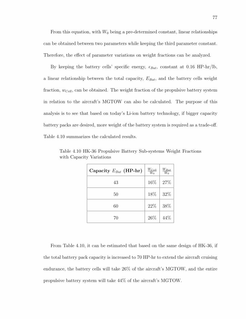
77

From this equation, with W0 being a pre-determined constant, linear relationships

can be obtained between two parameters while keeping the third parameter constant.

Therefore, the effect of parameter variations on weight fractions can be analyzed.

By keeping the battery cells’ specific energy, εBat, constant at 0.16 HP-hr/lb,

a linear relationship between the total capacity, EBat, and the battery cells weight

fraction, wCell, can be obtained. The weight fraction of the propulsive battery system

in relation to the aircraft’s MGTOW can also be calculated. The purpose of this

analysis is to see that based on today’s Li-ion battery technology, if bigger capacity

battery packs are desired, more weight of the battery system is required as a trade-off.

Table 4.10 summarizes the calculated results.

Table 4.10 HK-36 Propulsive Battery Sub-systems Weight Fractionswith Capacity Variations

Capacity EBat (HP-hr) WCell

W0

WBat

W0

43 16% 27%

50 18% 32%

60 22% 38%

70 26% 44%

From Table 4.10, it can be estimated that based on the same design of HK-36, if

the total battery pack capacity is increased to 70 HP-hr to extend the aircraft cruising

endurance, the battery cells will take 26% of the aircraft’s MGTOW, and the entire

propulsive battery system will take 44% of the aircraft’s MGTOW.

78

Keeping the battery pack capacity EBat at 43 HP-hr will enable the analysis

between battery cells specific energy εBat and the cells weight fractions. The purpose

of this analysis is to show that when designing battery packs with the same capacities,

the Li-ion battery technology improvement will directly help with lowering the weight

fractions of propulsive battery systems. Calculation results are shown in Table 4.11.

Table 4.11 HK-36 Propulsive Battery Sub-systems Weight Fractionswith Specific Energy Variations

Specific Energy εBat (HP-hr/lb) WCell

W0

WBat

W0

0.16 16% 27%

0.2 13% 22%

0.3 8% 15%

0.5 5% 9%

From Table 4.11, it can be estimated that based on the same design of the HK-

36, if the total Li-ion battery technology improvement doubles the specific energy

to 0.3 HP-hr/lb, the battery cells will take 8% of the aircraft’s MGTOW, and the

entire propulsive battery system will take 15% of the aircraft’s MGTOW. And if the

specific energy can be further increased to 0.5 HP-hr/lb, then the battery cells will

take 5% of the aircraft’s MGTOW, with the entire battery system only taking 9% of

the aircraft’s MGTOW.

79

5. Conclusion

5.1 Significant Results

An equivalent circuit model (ECM) of lithium-ion cells was selected to theoret-

ically model the batteries’ electrical behavior. The four internal parameter look-

up-tables that describe this ECM were estimated based on the NCR18650GA cells

experimental data. A lithium-ion single cell simulation model was developed to ac-

commodate the four parameter look-up-tables. The simulation model is then able to

simulate NCR18650GA battery cells behavior during discharge at 25oC. Validations

of the single cell simulation model with both constant discharging current and HK-36

flight mission profile show simulation errors less than 1.3%.

A recursive least squares (RLS) based real-time estimator was created to estimate

the battery pack’s SOC, SOH, and the remaining energy. It is exponentially conver-

gent with a forgetting factor λ (0 < λ ≤ 1). Given an input signal with persistent

excitation, this RLS based estimator is able to adaptively estimate one Li-ion cell’s

SOC, SOH, and the remaining energy in real time. The algorithm can also esti-

mate a battery pack’s remaining energy assuming that all cells connected in parallel

are identical. The validation results indicate that the RLS based estimator achieves

convergence within a very short time period (≈ 1 second) with desirable estimation

accuracy (normally under 1%). Additionally, the RLS based estimator can be applied

80

to any type or configuration of battery packs provided that OCV-SOC and Z-SOH

relations can be pre-determined.

The HK-36 propulsive battery system takes approximately 27% of the aircraft

gross weight. 58% of the battery system weight is the cells weight, and 42% is

the auxiliary components weight. Taking the weight fraction into consideration,

NCR18650GA cells effective specific energy reduces from 0.16 HP-hr/lb (259 W-

hr/kg) to 0.09 HP-hr/lb (150 W-hr/kg).

5.2 Future Work

The lithium-ion single cell simulation model developed in this thesis excludes any

thermal behavior of cells or any heat exchange with the ambient environment. Future

work should be done to expand the 2D parameter look-up-tables to 3D to include the

thermal effects by adding a third temperature axis.

Li-ion batteries have different performances when being charged and discharged.

In this thesis, all battery performance plots and internal parameter look-up-tables are

obtained in situations when the cells are being discharged. Future work would include

the battery charging performance by repeating the same experiments discussed in this

thesis, but under situations when the cells are being charged.

At the beginning of this thesis, the assumption is made that all cells connected

in parallel are identical. However, in real world cases, variations exist among cells

in parallel. This could result in different current splits and cause remaining energy

81

imbalances among them. To solve this problem, parameter variations among parallel

connected cells would be considered in future work.

From the input signal variations analysis in this research, no optimized excitation

amplitudes or frequencies were discovered, even though some excitations had better

estimation accuracies than others. More combinations of excitation amplitudes and

frequencies can be compared and analyzed in future work to determine how input

signal variances affect estimation accuracies.

Future research could also be done to decide if it is feasible to use the current rip-

ple from the motor controller caused by transistor switching as the system persistent

excitation for RLS estimation algorithm.

82

REFERENCES

Balas, M. (2017). Least squares notes.

Battery Bro. (2014, September). Inspecting the newpanasonic-sanyo ncr18650bf. Retrieved August, 2017, fromhttps://batterybro.com/blogs/18650-wholesale-battery-reviews/17840447-awesome-batteries-part-1-inspecting-the-new-panasonic-sanyo-ncr18650bf

Birkl, C. R., Roberts, M. R., McTurk, E., Bruce, P. G., & Howey,D. A. (2017, December). Degradation diagnostics for lithium ioncells. Journal of Power Sources , 341 , 373-386. Retrieved fromhttp://www.sciencedirect.com/science/article/pii/S0378775316316998

Chaoui, H., Golbon, N., Hmouz, I., Souissi, R., & Tahar, S. (2015, March). Lyapunov-based adaptive state of charge and state of health estimation for lithium-ionbatteries. IEEE Transactions on Industrial Electronics , 62 (3), 1610-1618. doi:10.1109/TIE.2014.2341576

Chevron Products Company. (2007). Aviation fu-els technical review. Retrieved August, 2017, fromhttps://www.cgabusinessdesk.com/document/aviation tech review.pdf

Diamond Aircraft. (1997, Mar). Airplane flight manual for the powered sailplane hk 36 ttc.Diamond Aircraft.

Gholizadeh, M., & Salmasi, F. R. (2014, March). Estimation of state of charge, unknownnonlinearities, and state of health of a lithium-ion battery based on a comprehensiveunobservable model. IEEE Transactions on Industrial Electronics , 61 (3), 1335-1344.doi: 10.1109/TIE.2013.2259779

Gibbs, B. P. (2011). Advanced kalman filtering, least-squares and modeling: A practicalhandbook (1st ed.). Wiley.

He, H., Xiong, R., & Fan, J. (2011, March). Evaluation of lithium-ion battery equivalentcircuit models for state of charge estimation by an experimental approach. Energies ,4 , 582-598. doi: 10.3390/en4040582

Huang, W., & Qahouq, J. A. A. (2014, November). An online battery impedance measure-ment method using dcdc power converter control. IEEE Transactions on IndustrialElectronics , 61 (11), 5987-5995. doi: 10.1109/TIE.2014.2311389

Huria, T., Ceraolo, M., Gazzarri, J., & Jackey, R. (2012). High fidelity electricalmodel with thermal dependence for characterization and simulation of high powerlithium battery cells. 2012 IEEE International Electric Vehicle Conference, 1-8. doi:10.1109/IEVC.2012.6183271

83

Johnstone, R. M., Johnson, C. R., Bitmead, R. R., & Anderson, B. D. O. (1982).Exponential convergence of recursive least squares with exponential forgetting fac-tor. 21st IEEE Conference on Decision and Control, Orlando, FL, 994-997. doi:10.1109/CDC.1982.268295

Karden, E., Buller, S., & Doncker, R. W. D. (2000). A method formeasurement and interpretation of impedance spectra for industrialbatteries. Journal of Power Sources , 85 , 72-78. Retrieved fromhttp://www.sciencedirect.com/science/article/pii/S0378775399003857

Lee, S., Kim, J., Lee, J., & B.H.Cho. (2008). State-of-charge and capac-ity estimation of lithium-ion battery using a new open-circuit voltage versusstate-of-charge. Journal of Power Sources , 185 , 1367-1373. Retrieved fromhttp://www.sciencedirect.com/science/article/pii/S0378775308017965

Panasonic. (2017). Specifications for ncr18650ga. Retrieved July, 2017, fromhttps://www.nkon.nl/sk/k/ncr18650ga.pdf

Rowell, D. (2008, Fall). 2.161 signal processing: Continuous and discrete. Retrieved fromhttp://ocw.mit.edu

Shell. (1999, February). Shell avgas 100ll piston en-gine aircraft fuel. Retrieved August, 2017, fromhttp://www.shell.com.au/motorists/shell-fuels/msds-tds/ jcr content/par/textimage 278c.stream/1468561712721/42cc39fc0b31146bc1c4d344c08422206521206f80d031b5f89f9b697c327c81/avgas-100ll-pds.pdf

Snihir, I., Rey, W., Verbitskiy, E., Belfadhel-Ayeb, A., & Notten, P. H.(2006). Battery open-circuit voltage estimation by a method of statisti-cal analysis. Journal of Power Sources , 159 , 1484-1487. Retrieved fromhttp://www.sciencedirect.com/science/article/pii/S0378775305016460

Standard Wire and Cable Co. (2017). Technical handbook and catalog (12th ed.). RetrievedAugust,2017, from http://www.standard-wire.com/downloads/swc catalog.pdf

Stroe, D.-I., Swierczynski, M., Kr, S. K., & Teodorescu, R. (2016). A comprehensivestudy on the degradation of lithium-ion batteries during calendar ageing: The internalresistance increase. 2016 IEEE Energy Conversion Congress and Exposition (ECCE),Milwaukee, WI, 2016 , 1-7. doi: 10.1109/ECCE.2016.7854664

Tripathy, Y., McGordon, A., Marco, J., & Gama-Valdez, M. (2014). State-of-charge estimation algorithms and their implications on cells in parallel. 2014IEEE International Electric Vehicle Conference (IEVC), Florence, 2014 , 1-6. doi:10.1109/IEVC.2014.7056168

United States Energy Information Administration. (2017, June).Monthly energy review june 2017. table 3.7c petroleum consump-tion: Transportation and electric power sectors. Retrieved fromhttps://www.eia.gov/totalenergy/data/monthly/pdf/sec3 21.pdf

United States Federal Aviation Administration. (2017). Faa aerospaceforecast (fiscal years 2017-2037). Retrieved July, 2017, fromhttps://www.faa.gov/data research/aviation/aerospace forecasts/media/FY2017-37 FAA Aerospace Forecast.pdf

84

Xiong, R., Sun, F., Gong, X., & He, H. (2013). Adaptive stateof charge estimator for lithium-ion cells series battery pack in electricvehicles. Journal of Power Sources , 242 , 699-713. Retrieved fromhttp://www.sciencedirect.com/science/article/pii/S0378775313008616

YASA Motors. (2017). Yasa 750. Retrieved July, 2017, fromhttp://www.yasamotors.com/wp-content/uploads/2014/07/Datasheet-YASA-750en-ID-15637.pdf