Autonomous Identification of Vertical Lines in Video

Autonomous Identification of Vertical Lines in Video Images to Assist in UGV Cover and Concealment

by William F. Oberle

ARL-TR-3365 November 2004 Approved for public release; distribution is unlimited.

NOTICES

Disclaimers The findings in this report are not to be construed as an official Department of the Army position unless so designated by other authorized documents. Citation of manufacturer’s or trade names does not constitute an official endorsement or approval of the use thereof. DESTRUCTION NOTICE Destroy this report when it is no longer needed. Do not return it to the originator.

Army Research Laboratory Aberdeen Proving Ground, MD 21005-5066

ARL-TR-3365 November 2004


William F. Oberle

Weapons and Materials Research Directorate, ARL Approved for public release; distribution is unlimited.

ii

REPORT DOCUMENTATION PAGE Form Approved OMB No. 0704-0188

Public reporting burden for this collection of information is estimated to average 1 hour per response, including the time for reviewing instructions, searching existing data sources, gathering and maintaining the data needed, and completing and reviewing the collection information. Send comments regarding this burden estimate or any other aspect of this collection of information, including suggestions for reducing the burden, to Department of Defense, Washington Headquarters Services, Directorate for Information Operations and Reports (0704-0188), 1215 Jefferson Davis Highway, Suite 1204, Arlington, VA 22202-4302. Respondents should be aware that notwithstanding any other provision of law, no person shall be subject to any penalty for failing to comply with a collection of information if it does not display a currently valid OMB control number. PLEASE DO NOT RETURN YOUR FORM TO THE ABOVE ADDRESS.

1. REPORT DATE (DD-MM-YYYY ) November 2004

2. REPORT TYPE

Final 3. DATES COVERED (From - To)

April 2004 to September 2004 5a. CONTRACT NUMBER

5b. GRANT NUMBER

4. TITLE AND SUBTITLE


5c. PROGRAM ELEMENT NUMBER

5d. PROJECT NUMBER

622618AH03 5e. TASK NUMBER

6. AUTHOR(S)

William F. Oberle (ARL)

5f. WORK UNIT NUMBER

7. PERFORMING ORGANIZATION NAME(S) AND ADDRESS(ES)

U.S. Army Research Laboratory Weapons and Materials Research Directorate Aberdeen Proving Ground, MD 21005-5066

8. PERFORMING ORGANIZATION REPORT NUMBER

ARL-TR-3365 10. SPONSOR/MONITOR'S ACRONYM(S) 9. SPONSORING/MONITORING AGENCY NAME(S) AND ADDRESS(ES)

11. SPONSOR/MONITOR'S REPORT NUMBER(S)

12. DISTRIBUTION/AVAILABILITY STATEMENT

Approved for public release; distribution is unlimited.

13. SUPPLEMENTARY NOTES

14. ABSTRACT

The autonomous identification of appropriate locations that provide cover and concealment for a robotic vehicle is a difficult task. Fortunately, many appropriate locations are man-made and are characterized by a distinctive geometric characteristic, specifically, object edges that form vertical straight lines. The objective of this report is to propose, implement, and assess an algorithm for the autonomous identification of vertical lines in video images that offer the most appropriate location for cover and concealment. Results obtained from the application of the algorithm to a number of video sequences indicate that the algorithm is effective in identifying acceptable locations. Several areas for improvement of the algorithm are suggested and discussed.

15. SUBJECT TERMS

canny edge detector; edge detection; Hough transform; UGV

16. SECURITY CLASSIFICATION OF: 19a. NAME OF RESPONSIBLE PERSON

William F. Oberle a. REPORT

Unclassified b. ABSTRACT

Unclassified c. THIS PAGE

Unclassified

17. LIMITATIONOF ABSTRACT

UL

18. NUMBER OF PAGES

25

19b. TELEPHONE NUMBER (Include area code)

410-278-4362 Standard Form 298 (Rev. 8/98)

Prescribed by ANSI Std. Z39.18

iii

Contents

List of Figures iv

List of Tables iv

Acknowledgments v

1. Introduction 1

2. Nearest Vertical Line Detector (NVLD) Algorithm 2 2.1 Task 1 ..............................................................................................................................2 2.2 Task 2 ..............................................................................................................................9 2.3 Step 3.............................................................................................................................10

3. Application to Video Sequences 11 3.1 VS1: Video Sequence 1................................................................................................11 3.2 VS2: Video Sequence 2................................................................................................14

4. Conclusions and Future Work 17

5. References 19

Distribution List 20

iv

List of Figures

Figure 1. Outdoor scene with natural and man-made features. ......................................................1 Figure 2. Discrete gradient directions. ...........................................................................................4 Figure 3. Results of Canny edge detection: original image (left); edges with t(high) = 0.95

(center); edges with t(high) = 0.5..............................................................................................5 Figure 4. Example of Hough transform algorithm..........................................................................6 Figure 5. Polar representation of a line. ..........................................................................................6 Figure 6. Schematic of image coordinate system with the polar representation of an arbitrary

line..............................................................................................................................................7 Figure 7. Illustration of range of lines that will be considered vertical. .........................................7 Figure 8. Possible orientations of line to vertical, clockwise (left) and counterclockwise

(right), illustrating that the angle with the vertical is equal to the parameter θ. .......................8 Figure 9. Illustration of the geometry associated with the condition used to determine ∆θ...........8 Figure 10. Valid (left) and invalid (right) line segments. ..........................................................10 Figure 11. Video sequence VS1....................................................................................................12 Figure 12. Edges in VS1 as determined by the Canny edge detector component of the NVLD

procedure..................................................................................................................................13 Figure 13. Grey scale of VS1 with dominant vertical line inserted. (Bottom of dominant

vertical line indicated by red arrow.) .......................................................................................14 Figure 14. Video sequence VS2....................................................................................................15 Figure 15. Edges in VS2 as determined by the Canny edge detector component of the NVLD

procedure..................................................................................................................................16 Figure 16. VS2 grey scale and dominant vertical lines. (Bottom of dominant vertical line

indicated by red arrow.) ..........................................................................................................17

List of Tables

Table 1. Input parameters for vertical line procedure...................................................................10

v

Acknowledgments

The author would like to thank Dr. MaryAnne Fields of the U.S. Army Research Laboratory for her time and effort in reviewing the report. Her comments and suggestions proved valuable in the preparation of the final version of the report. Additionally, the author would like to thank Dr. Fields for her suggestions and discussions concerning various algorithms for selecting lines closest to the video camera.

vi

INTENTIONALLY LEFT BLANK

1

1. Introduction

Many tactical Army missions require the use of natural and man-made features in the environment for cover and concealment from the enemy. For humans, it is a fairly straightforward process to identify features offering adequate cover and concealment in the operating environment, when it exists. However, for an unmanned ground vehicle (UGV) operating autonomously (i.e., no human intervention), the problem of finding adequate cover and concealment is extremely difficult. The UGV must rely solely on its on-board sensors and a priori map data to find and assess potential features offering adequate cover. In addition, the entire process (data acquisition and assessment) must be automated. One approach is to mimic the steps performed by a human that essentially involve visually inspecting the environment for appropriate features, assessing the worth of each location (based on experience), and selecting the most promising ones. The objective of this report is to propose, implement, and assess an algorithm that would permit a UGV or other unmanned vehicle to autonomously perform this action.

As detailed in section 2, the proposed algorithm will rely upon the identification of vertical lines in video images captured by the vehicles’ on-board camera(s). However, the use of vertical lines may restrict the type of features that can be located. Most natural features used for cover and concealment (e.g., hills, tree lines, gullies, etc.) are often irregularly shaped. On the other hand, almost all man-made and some natural (e.g., tree trunks) features have distinct geometric profiles. A predominant characteristic of these distinct geometric profiles is the inclusion of vertical edges that form straight lines. This is illustrated in figure 1 in which natural and man-made features are shown. Vertical edges forming lines for the man-made features (building, telephone poles in the foreground and background, door and window) are clear, while the tree line exhibits almost no vertical edges forming lines. Thus, using the presence of vertical lines in a feature’s profile will most likely identify man-made objects.

Figure 1. Outdoor scene with natural and man-made features.

2

The remainder of this report is organized as follows. In section 2, the proposed algorithm for identifying, assessing, and selecting the vertical line in a video image corresponding to a likely location for cover and concealment is described. Application of the algorithm to several video sequences and an assessment of the results are provided in section 3. Conclusions and future work are discussed in the final section.

2. Nearest Vertical Line Detector (NVLD) Algorithm

As just discussed, the NVLD algorithm must accomplish three separate tasks. First, vertical lines must be identified in the video image. Fortunately, edge finding and line identification is a classic problem in machine vision. The Canny edge detector (Canny, 1986; Faugeras, 1993; Trucco & Verri, 1998) and Hough transform (Klaus & Horn, 1986; Faugeras, 1993; Jahne, 1997; Trucco & Verri, 1998) approach is used as the basis for the algorithm developed in this report. The Canny edge detector is selected on the basis of a review of the machine vision literature (see Heath, Sarkar, Sanocki, & Bowyer, 1998, for a summary). Source code obtained from Heath’s web site (Heath, 2004) is used together with a version of the Hough transform written by the author for identifying lines within a user-specified angle, ±SkewAngle, to the vertical. A value of ±0.1745 radian (10 degrees) (i.e., a line making an angle between 1.39626 and 1.745329 radians [80 and 100 degrees] with the horizontal) is used in this report. The second task involves assessing the set of vertical lines identified in the first task to determine if the lines could be part of features that could offer acceptable cover and concealment. For this report, the assessment is based on continuous line length.1 The final task is the selection of the single vertical line judged to offer the most appropriate cover and concealment location. Assuming success of the second task, the selection is based on identification of the vertical line closest to the video camera. This corresponds to using the cover and concealment location closest to the vehicle. Details of each task are provided in the remainder of this section.

2.1 Task 1

Identifying vertical lines in an image can be decomposed into two distinct steps. First, we determine all pixels in the image that correspond to edges2 and, second, we identify vertical lines based on evidence provided by the edge pixels. Step 1 is performed with the Canny edge detector and step 2 is accomplished with a Hough transform.

1In this report, continuous lines may have gaps, as discussed in section 2.2. 2Edge points (pixels), or edges, are pixels at or around which the image values undergo a sharp variation (Trucco

& Verri, 1998). Image values refer to the numeric value(s) assigned to each pixel used to denote the color of the pixel. Many color models are currently used in machine vision, depending on the application. Grey scale and RGB (red, blue, green) are the two models used in this report.

3

A brief description of the Canny edge detector, following the approach of Trucco and Verri (1998) and Heath (2004), is provided to acquaint the reader with the parameters that must be specified in order to execute the algorithm and the impact that these parameters have on the algorithm’s results.

From a mathematical perspective, an image can be viewed as a contour map. Thus, at any point in the image, the gradient indicates the direction of the most rapid variation in image values, and the magnitude of the gradient measures the severity of the variation. However, before the gradient is computed, several issues must be addressed. First, video images are generally corrupted by acquisition noise. To reduce the impact of such noise, the image should be filtered or smoothed. Without specific knowledge of the noise distribution, it is generally assumed that the noise is white3 with a Gaussian distribution. Thus, Gaussian smoothing is used to reduce the impact of noise, and, since the image is discrete, a discretized Gaussian filter is used. A contin-uous Gaussian distribution is defined by its mean and standard deviation. The white noise assumption implies that the mean should be zero. Thus, the Gaussian in this case is defined by its standard deviation, which for the discrete Gaussian filter corresponds to the window size of the filter. In Heath’s implementation, the Gaussian standard deviation is an input parameter and the Gaussian filter window size is determined by

in which σ = the Gaussian standard deviation. Since the objective is to identify sharp changes in the image values, the window size should be as small as possible but still filter the noise. For the images used in this report, acquisition noise is not a problem and σ is set equal to 0.25, resulting in a window size of 3 for the Gaussian filter. The second issue involves the image values. A numerical computation of the gradient requires a single-value function. If the image uses the grey scale color model, this condition is satisfied. However, if the RGB color model is used, each pixel has three image values and the image value function is multi-valued. In order to compute the gradient in this case, only one of the color channels (red, green, or blue) can be used, or the image can be converted to grey scale. Both approaches are available in the procedure as options to the user. The conversion from the RGB color model to a grey scale color model is accom-plished with the “luma” (Poynton, 1996) formula defined by

Grey = 0.299 * Red + 0.587 * Green + 0.114 * Blue.

Once the gradient is computed at each pixel, the natural next step would be to scan the pixels and identify as edge points all pixels for which the magnitude of the gradient exceeds some threshold value. However, this approach can result in thick edges (i.e., greater than 1 pixel) being identified in the image. Ideally, the edges should be 1 pixel wide. The Canny edge detector ensures that all edges are 1 pixel wide by employing a process referred to as non-maximum suppression. Non-

3White noise is defined as noise with a frequency spectrum that is uniform and continuous over a specified

frequency band.

Window Size = ceiling1 2 2 5+ * . * ,σb g

4

maximum suppression is based on the fact that the gradient vector is normal to an edge, and thus, the width of the edge is in the direction of the gradient. To perform non-maximum suppression, each pixel in the image is analyzed to determine if it is the dominant edge pixel. Consider figure 2 and suppose that the pixel labeled A is being analyzed. The direction of the gradient is between 0 and 2π radians (0 and 360 degrees). Select the direction that best approximates the gradient from among the eight directions shown in the figure. Along this and the opposite direction, the pixel labeled A has two neighbors. If the magnitude of the gradient of the pixel labeled A is smaller than either of these two neighbors, we set the gradient of the pixel labeled A to zero (nonmaximum suppression); otherwise, we leave the value of the gradient unchanged. The results are stored in an image labeled G (i.e., G[i,j] = magnitude of the gradient for the pixel at location [i,j] or 0 if the pixel is suppressed). Once non-maximum suppression is completed, the edges can be identified. However, simply marking as an edge pixel every pixel with a gradient magnitude greater than some threshold value can result in streaking (fragmented edges) and does not provide information about which edge pixels are connected. The Canny edge detector overcomes these problems through what is termed “hysteresis thresholding,” which requires two input parameters, Tlow and Thigh with Tlow < Thigh.

Figure 2. Discrete gradient directions.

Assuming that a specific order for visiting each element of G(i,j) is defined, then the basic algorithm for hysteresis thresholding is (Trucco & Verri, 1998):

1. Locate the next unvisited edge pixel, G(i,j), so that G(i,j) > Thigh.

2. Starting from G(i,j), follow the chains of connected local maximum (G ≠ 0), in both directions perpendicular to the edge normal, as long as G > Tlow. Mark all visited points as being part of a connected edge.

In effect, Thigh is the threshold value to start an edge while Tlow is the threshold value to continue the edge. To make his program more flexible, Heath introduces two new parameters, thigh and tlow, from which Thigh and Tlow are computed. The input values for thigh and tlow are between 0 and 1 with thigh > tlow. The values for Thigh and Tlow are then determined on the basis of the distribution of the magnitudes of the gradient for the image being analyzed. The input thigh and tlow are multiplied by 100, and Thigh and Tlow are the percentile values associated with the distribution of the magnitudes of the gradient at the values thigh and tlow (e.g., if the input value of thigh is 0.78, the

A

5

Thigh value corresponds to the 78th percentile of the gradient magnitudes). The larger the value of Thigh/thigh, the fewer the number of edge pixels that will be considered as starting locations for connected edges. In addition, since the magnitude of the gradient is greatest when there is a large difference in the image values, the potential starting pixels for outdoor scenes will tend to favor objects in which the sky is the background. These observations are illustrated in figure 3.

Figure 3. Results of Canny edge detection: original image (left); edges with t(high) = 0.95 (center); edges with t(high) = 0.5.

Of particular interest is the failure to identify the telephone pole in the foreground when Thigh = 0.95.

Following hysteresis thresholding, a binary image (edges denoted by black) of the connected edges (center and right of figure 3) is constructed. This completes a brief description of the Canny edge detector.

As illustrated in figure 3, the Canny edge detector identifies connected edges, regardless of shape. The Hough transform is used to isolate those edges corresponding to vertical or near vertical lines as discussed previously. Essentially, the Hough transform is a voting algorithm based on the evidence provided by the input data. To illustrate the basic idea of Hough transform, consider figure 4. The blue dots in the figure represent four points that are the input and the question to be answered is “What line goes through the most points?” One way to characterize lines is through the use of slope (m) and y-intercept (b). Suppose that it is known that the slope and y-intercept for the desired line are bound; then these bound intervals can be discretized to create a finite two-dimensional array (counter array) where each cell corresponds to a (m,b) pair. (For the sake of simplicity, assume that the slopes and y-intercepts for the lines in figure 4 all have a corresponding cell in the array.) Now for each input point, step through all possible discrete slopes and determine the nearest discrete y-intercept. Increase the appropriate counter array cell by 1. For the example in figure 4, after all input points are considered, cell (m1,b1) has a count of 3 (i.e., three points are on this line), cells (m2,b2), (m3,b3), and (m4,b4) have a count of 2, while all the other cells have a count of 1 or 0. This mapping from the original information to the counter array space is the Hough transform. The counter array cell with the highest count is the desired answer.

Unfortunately, using slope and y-intercept to parameterize lines is a poor choice when we are using the Hough transform since both parameters are unbound. To overcome this difficulty, the

Ml

^T

6

polar representation, ρ = x cos θ + y sin θ, for a line is used, in which ρ is the distance from the coordinate axes origin to the line, while θ is the angle between the x-axis and the vector perpendicular to the line (see figure 5).

Figure 4. Example of Hough transform algorithm.

Figure 5. Polar representation of a line.

To apply the Hough transform to identify vertical lines in an image, the discretization of the parameters ρ and θ must be determined. If C is the number of columns and R the number of rows in the image, c = C – 1, and r = R – 1, then a schematic of the image and the orientation of ρ and θ for an arbitrary line in the image are shown in figure 6. As stated earlier, a line will be considered to be vertical if it is within plus or minus a user-specified angle (SkewAngle) to the vertical, as illustrated in figure 7.

y = m3x + b3

y = m2x + b2

y = m4x + b4

y = m1x + b1

y = m3x + b3

y = m2x + b2

y = m4x + b4

y = m1x + b1

ρ

θ

ρ

θ

7

Figure 6. Schematic of image coordinate system with the polar representation of an arbitrary line.

Figure 7. Illustration of range of lines that will be considered vertical.

Fortunately, the angle a line makes with the vertical is the same as the parameter θ, as illustrated in figure 8. In the figure, the two possible cases for vertical lines, either clockwise (left) or counterclockwise (right) to the vertical, are shown. For the clockwise orientation, ∆ABC ~ ∆BDC (i.e., similar triangles). While for the counterclockwise orientation, ∆ABC ~ ∆EDC. In either case, the angle with the vertical is equal to the angle defined by θ.

ρ

θ

(0,r) (c,r)

(c,0)(0,0)

Image

ρ

θ

(0,r) (c,r)

(c,0)(0,0)

Image

(0,r) (c,r)

(c,0)(0,0)

Image

SkewAngle

(0,r) (c,r)

(c,0)(0,0)

Image

SkewAngle

8

Figure 8. Possible orientations of line to vertical, clockwise (left) and counterclockwise (right), illustrating that the angle with the vertical is equal to the parameter θ.

It is now possible to define how ρ and θ are discretized. The line that is the greatest distance from the origin of the image passes through the lower right point of the image (i.e., point (c,r)) and forms an angle of SkewAngle radians clockwise from the vertical. Thus, the maximum value for ρ is given by the expression

ρmax = c * cos(SkewAngle) + r * sin(SkewAngle).

Rounding ρmax to the next highest integer and letting the step size equal 1, the discretization of ρ is complete. Unlike ρ, the maximum value θ is known (i.e., SkewAngle) and it is the step size that must be determined. Any number of criteria can be used, but for this report, the angle step size ∆θ is chosen so that two lines passing through (c,r) with orientations SkewAngle and SkewAngle-∆θ will intersect the top edge of the image in adjacent pixels (see figure 9).

Figure 9. Illustration of the geometry associated with the condition used to determine ∆θ.

E

D C

B

A D C

BA

θθ

ρmax

∆θ

(0,r) (c,r)

(c,0)(0,0)

Image

SkewAngle

OnePixel

ρmax

∆θ

(0,r) (c,r)

(c,0)(0,0)

Image

SkewAngle

OnePixel

9

With the notation in figure 9, the condition for determining ∆θ is

ρmax – (c + r tan(SkewAngle - ∆θ) = 1. Solving for θ∆ ,

∆θ = θ - tan-1 ((ρmax - c – 1)/r)

With ρ and θ discretized, the counter array is constructed and the Hough transform of the binary edge image (produced by the Canny edge detector) is performed. The final step in identifying the vertical lines is to determine those cells in the counter array that exceed a user-specified threshold (i.e., how many edge points must be on a given line to consider that line to be in the image). This provides the set of vertical lines for the second task.

2.2 Task 2 This task involves evaluating the identified vertical lines to determine if any represents the edge of an object that can be used for cover and concealment. The assumption used to make this determination is that if a vertical line has sufficient length, then it corresponds to an acceptable object. In this case, sufficient length refers to a continuous length (i.e., a series of adjacent pixels with small user-defined gaps). The threshold value used in the Hough transform to identify vertical lines specifies the minimum number of pixels, labeled as edge pixels, necessary to indicate that a particular vertical line is present in the image (i.e., minimum number of edge pixels satisfying the equation of the line). Unfortunately, this can result in false positives, i.e., lines being identified as part of the image when they are not actually present. For example, consider an image consisting of horizontal lines in every third scan line. This image contains no vertical lines. However, in the Hough transform, every counter array cell corresponding to a vertical line will have a count equal to one-third the number of scan lines. Thus, a test to determine if an identified vertical line is actually in the image must be performed. The deter-mination if a specific line is present in the image and test for a continuous run of edge pixels can be combined into a single test. The basic approach is to determine if there is a sufficient run of adjacent pixels on the line. Unfortunately, simply checking for adjacent pixels is insufficient since the original image can be corrupted by noise. To account for potential noise, two user-supplied parameters are used. The first parameter, iLineMin, specifies the minimum number of adjacent pixels, not counting gaps, that must be present for a vertical line to be present in the image and represent the edge of an acceptable object. The second parameter, iGapMax, is the maximum number of pixels that can be considered as a gap in a legitimate line segment. For example, if iLineMin = 6 and iGapMax = 2, then in figure 10, the pixels on the left form an acceptable vertical line while those on the right do not. One final parameter is required. Depending on the camera and how the image is acquired, the left or right edge of the image may contain a region where all the pixels are black, e.g., left side of image, figure 3 (left-most image). This corresponds to a vertical line in the edge detection as shown in figure 3 (center and right-most images). To avoid considering this false vertical line the final parameter, iBorder specifies the number of pixels to be ignored on the left and right border of the image.

10

Figure 10. Valid (left) and invalid (right) line segments.

2.3 Task 3

In task 3 a single vertical line (dominant vertical line) must be selected from the vertical lines identified in the second task. The criterion for the algorithm is to select the closest vertical line to the video camera. Dr. MaryAnne Fields, U.S. Army Research Laboratory, suggested that this corresponds to selecting that vertical line that terminates lowest in the image, i.e., the vertical line whose bottom pixel has the largest row index. This approach is implemented in the algo-rithm. First, the end point of each candidate vertical line segment must be determined. We accomplish this by extending the method used in step 2 to determine acceptable vertical lines. Specifically, the end point for a line segment is the pixel so that

1. It is a continuous part of the line as described above, and

2. No other pixel that is a continuous part of the line has a higher row index.

Once the end point of each vertical line is determined, a straightforward search for the vertical line whose end point has the highest row index is performed to identify the single vertical line required of the algorithm.

A total of eight parameters must be provided by the user in order to run the algorithm. These parameters depend on the camera and data acquisition hardware used to obtain the images analyzed by the procedure. Table 1 lists the eight parameters, describes their use, and gives the values used in section 3 of this report to analyze several video sequences.

Table 1. Input parameters for vertical line procedure

Parameter Description Values Use in Section 3

dSigma Standard deviation used in Gaussian filter (Canny edge detector) 0.25 dTHigh Upper threshold in hystersis threshold (Canny edge detector) 0.5 dTLow Lower threshold in hystersis threshold (Canny edge detector) 0.1

SkewAngle Maximum angle that a vertical line can make with vertical (Hough transform) 0.1745329252 (radian), or 10 (degrees)

iThreshold Minimum counter array value to consider entry a vertical line (Hough transform) 50 iLineMin Minimum number of continuous pixels required to determine an acceptable line (step 2, assessment of vertical lines) 10 iGapMax Maximum number of pixels that can occur in a gap of continuous pixels (step 2, assessment of vertical lines) 3 iBorder Number of pixels to be ignored on the left and right sides of an image (step 2, assessment of vertical lines) 15

11

3. Application to Video Sequences

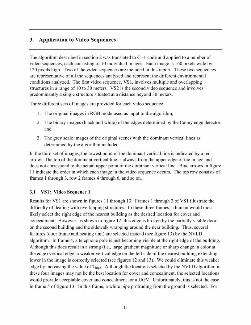
The algorithm described in section 2 was translated to C++ code and applied to a number of video sequences, each consisting of 10 individual images. Each image is 160 pixels wide by 120 pixels high. Two of the video sequences are included in this report. These two sequences are representative of all the sequences analyzed and represent the different environmental conditions analyzed. The first video sequence, VS1, involves multiple and overlapping structures in a range of 10 to 30 meters. VS2 is the second video sequence and involves predominantly a single structure situated at a distance beyond 30 meters.

Three different sets of images are provided for each video sequence:

1. The original images in RGB mode used as input to the algorithm,

2. The binary images (black and white) of the edges determined by the Canny edge detector, and

3. The grey scale images of the original scenes with the dominant vertical lines as determined by the algorithm included.

In the third set of images, the lowest point of the dominant vertical line is indicated by a red arrow. The top of the dominant vertical line is always from the upper edge of the image and does not correspond to the actual upper point of the dominant vertical line. Blue arrows in figure 11 indicate the order in which each image in the video sequence occurs. The top row consists of frames 1 through 3, row 2 frames 4 through 6, and so on.

3.1 VS1: Video Sequence 1

Results for VS1 are shown in figures 11 through 13. Frames 1 through 3 of VS1 illustrate the difficulty of dealing with overlapping structures. In these three frames, a human would most likely select the right edge of the nearest building as the desired location for cover and concealment. However, as shown in figure 12, this edge is broken by the partially visible door on the second building and the sidewalk wrapping around the near building. Thus, several features (door frame and heating unit) are selected instead (see figure 13) by the NVLD algorithm. In frame 4, a telephone pole is just becoming visible at the right edge of the building. Although this does result in a strong (i.e., large gradient magnitude or sharp change in color at the edge) vertical edge, a weaker vertical edge on the left side of the nearest building extending lower in the image is correctly selected (see figures 12 and 13). We could eliminate this weaker edge by increasing the value of Thigh. Although the locations selected by the NVLD algorithm in these four images may not be the best location for cover and concealment, the selected locations would provide acceptable cover and concealment for a UGV. Unfortunately, this is not the case in frame 5 of figure 13. In this frame, a white pipe protruding from the ground is selected. For

12

the final five frames, the most appropriate location is selected (assuming that a telephone pole is acceptable cover and concealment). In general, the results of applying the NVLD algorithm to VS1 indicate that the NVLD algorithm performs well in indicating the location of acceptable cover and concealment for the environment shown in the video sequence. The results also suggest that the algorithm could be improved by the incorporation of procedures into the algorithm concerning object width to eliminate such objects as the pipe selected in frame 5.

Figure 11. Video sequence VS1.

■Jon» .

13

Figure 12. Edges in VS1 as determined by the Canny edge detector component of the NVLD procedure.

14

Figure 13. Grey scale of VS1 with dominant vertical line inserted. (Bottom of dominant vertical line indicated by red arrow.)

3.2 VS2: Video Sequence 2

Results for VS2 are shown in figures 14 through 16. In general, VS2 involves a single structure in each image. Except for the first frame, the procedure performs well in selecting appropriate locations for cover and concealment (see figure 16). In figure 15, note that the discoloration of the metal building (figure 14, frame 1) causes this building to have many broken edges and a “scaly” look compared to the building on the left side of the images (when present). It is these broken edges that prevent an edge of the building from being selected in frame 1.

15

Figure 14. Video sequence VS2.

16

Figure 15. Edges in VS2 as determined by the Canny edge detector component of the NVLD procedure.

17

Figure 16. VS2 grey scale and dominant vertical lines. (Bottom of dominant vertical line indicated by red arrow.)

4. Conclusions and Future Work

An algorithm for the autonomous identification of locations offering acceptable cover and con-cealment for a UGV, based on the presence of vertical lines (edges) in a video image has been presented. The procedure is based on the Canny edge detector and Hough transform for identification of vertical lines, continuous line length to further restrict the set of vertical lines and selection of the nearest vertical line as the acceptable location. An analysis of the results of

18

applying the algorithm to a number of video sequences indicates that the procedure is effective in identifying acceptable locations.

Two areas where the algorithm should be improved in future efforts are suggested from the analysis supporting this report. The first area concerns the merging of edges when structures overlap. For example, in figure 11, frame 3, the right edge of the building in the foreground merges with the edge of the door frame of the building in the background to form a non-vertical edge. Since the resulting edge is no longer vertical, it is dropped from consideration by the procedure. Yet, it is exactly this corner of the building in the foreground that offers the best location for cover and concealment. One approach to address this problem is to combine depth information, especially depth discontinuity location, with the edge analysis. The second area for improvement concerns elimination of the selection of locations associated with the vertical edge of a thin or narrow object. Thin objects are generally not suitable for cover and concealment but they may have strong vertical edges (e.g., the pipe selected in figure 11, frame 5). Unfortunately, determining the width of an object in an image is difficult. A possible approach is to start by using color segmentation to determine the width of the object in pixels and then use depth information and camera characteristics to convert width in pixels to physical measurements.

19

5. References

Canny, J. A Computational Approach to Edge Detection. IEEE Transactions on Pattern Analysis and Machine Intelligence November 1986, 8 (6).

Faugeras, O. Three-Dimensional Computer Vision A Geometric Viewpoint, The MIT Press, Cambridge, Massachusetts, 1993.

Heath, M. Computer Vision Laboratory, University of South Florida, [email protected], 2004.

Heath, M.; Sarkar, S.; Sanocki, T.; Bowyer, K. Comparison of Edge Detectors, A Methodology and Initial Study. Computer Vision and Image Understanding January 1998, 69 (1), 38 – 54.

Jahne, B. Digital Image Processing Concepts, Algorithms, and Scientific Applications, Springer-Verlag, Berlin, Heidelberg, New York, 1997.

Klaus, B.; Horn, P. Robot Vision, The MIT Electrical and Engineering and Computer Science Series, The MIT Press, McGraw-Hill Book Company, New York, New York, 1986.

Poynton, C. A Technical Introduction to Digital Videl, John Wiley & Sons, New York, 1996.

Trucco, E.; Verri, A. Introductory Techniques for 3-D Computer Vision, Prentice Hall, 1998.

20

NO. OF COPIES ORGANIZATION * ADMINISTRATOR DEFENSE TECHNICAL INFO CTR ATTN DTIC OCA 8725 JOHN J KINGMAN RD STE 0944 FT BELVOIR VA 22060-6218 *pdf file only 1 DIRECTOR US ARMY RSCH LABORATORY ATTN IMNE AD IM DR MAIL & REC MGMT 2800 POWDER MILL RD ADELPHI MD 20783-1197 1 DIRECTOR US ARMY RSCH LABORATORY ATTN AMSRD ARL CI OK TECH LIB 2800 POWDER MILL RD ADELPHI MD 20783-1197 2 DIRECTOR US ARMY RSCH LABORATORY ATTN AMSRD ARL SE SE P GILLESPIE N NASRABADI 2800 POWDER MILL RD ADELPHI MD 20783-1197 1 NATL INST OF STDS & TECHNOLOGY ATTN DR M SHNEIER BLDG 200 GAITHERSBURG MD 20899 2 UNIV OF MARYLAND INST FOR ADV COMPUTER STUDIES ATTN DR L DAVIS D DEMENTHON COLLEGE PARK MD 20742-3251 ABERDEEN PROVING GROUND 1 DIRECTOR US ARMY RSCH LABORATORY ATTN AMSRD ARL CI OK (TECH LIB) BLDG 4600 2 DIRECTOR US ARMY RSCH LABORATORY ATTN AMSRD ARL WM J SMITH T ROSENBERGER BLDG 4600 2 DIRECTOR US ARMY RSCH LABORATORY ATTN AMSRD ARL WM B W CIEPIELLA BLDG 4600

NO. OF COPIES ORGANIZATION 16 DIRECTOR US ARMY RSCH LABORATORY ATTN AMSRD ARL WM BF H EDGE M BARANOSKI P FAZIO M FIELDS G HAAS (4 CYS) T HAUG W OBERLE (4 CYS) R PEARSON R VON WAHLDE S WILKERSON BLDG 390 2 DIRECTOR US ARMY RSCH LABORATORY ATTN AMSRD ARL WM RP C SHOEMAKER J BORNSTEIN BLDG 1121

Documents

Autonomous Identification of Vertical Lines in Video