EVALUATION OF ADVANCED RECEIVER AUTONOMOUS

INTEGRITY MONITORING FOR VERTICAL GUIDANCE USING

GPS AND GLONASS SIGNALS

A THESIS

SUBMITTED TO THE DEPARTMENT OF ELECTRICAL ENGINERRING

AND THE COMMITTEE ON GRADUATE STUDIES

OF STANFORD UNIVERSITY

IN PARTIAL FULFILLMENT OF THE REQUIREMENTS

FOR THE DEGREE OF

ENGINEER

Myungjun Choi

December 2014

© Copyright by Myungjun Choi 2014

All Right Reserved

iii

Myungjun Choi

Approved for the department:

__________________________________

(Per Enge) Adviser

Approved for the Stanford University Committee on Graduate Studies.

__________________________________

iv

v

Abstract

The Global Navigation Satellite System (GNSS) environment has experienced two major

transformations. First, fully operational constellations, including the United States Global

Positioning System (GPS) and Russian Global'naya Navigatsionnaya Sputnikovaya Sistema

(GLONASS), are in the middle of modernization plans. Specifically, these core constellations

will transmit new signals in new frequencies. Second, two more major GNSS constellations

are being launched and will be fully operational in the near future. They are the European

Galileo and Chinese Beidou systems. The new constellations' navigation signals will be

transmitted in multiple frequency bands as well. Therefore, GNSS users will experience more

signals and more satellites in the next five to ten years. In addition, these new signals will be

available for civil aviation navigation systems. Signals in dual frequencies allow receivers to

mitigate the pseudorange errors originating from the ionosphere. Moreover, more satellites

and multiple constellations provide users with better accuracy and position estimates. Through

these advantages, we can expect performance improvement in the navigation systems in terms

of accuracy, robustness, and integrity. Specifically, these advantages would lead GNSS

receivers to the possible use of Advanced Receiver Autonomous Integrity Monitoring

vi

(ARAIM), which is an extension of Receiver Autonomous Integrity Monitoring, which has

been in use in civil aviation for over twenty years for horizontal guidance. ARAIM would

extend RAIM to more demanding operations, in particular vertical guidance in landing

approaches. Hence, several ARAIM algorithms have been proposed and studied in order to

achieve global coverage of LPV-200 approaches, which guide an aircraft down to altitudes of

200 feet. The main purposes of this thesis are to introduce the multi-constellation ARAIM

algorithm and its tool, and present extensive evaluation work of the multi-constellation

ARAIM tool using real GPS and GLONASS signals.

The first part of this thesis explains the navigation requirement to support LPV-200

approaches and specifies the threats that might lead the navigation function into a hazardous

situation. ARAIM is designed to guarantee system integrity and assures that the navigation

system is operating appropriately. In this chapter the requirements in terms of positioning

performance (accuracy), integrity, continuity, and availability are specified through the

probability of hazardously misleading information (PHMI), the false alert probability, the

Vertical Position Error (VPE), and the Vertical Protection Level (VPL). According to LPV-

200 requirements, any situation that leads to not meeting the requirements are considered as a

threat. A threat can be caused by system status (faults), adverse weather, and intentional radio

frequency interference. This thesis mostly focuses on faults within the navigation system, and

describes what causes GNSS faults as well as their effects on a system.

The second part of this thesis describes the ARAIM user algorithm including the

characterization of satellite ranging error, fault detection and exclusion, and computing the

VPL. The error in the range measurement is the sum of error components and these errors are

modeled as a random variable and a bias. The first section specifies how to model each error

component with given satellite pseudorange. The second section describes the concept and

vii

architecture of the multi-constellation ARAIM algorithm. Multi-constellation issues will be

addressed as well.

The third part of this thesis demonstrates the results of the evaluation of multi-constellation

ARAIM. In order to assure possible use of multi-constellation ARAIM, it is necessary to test

this algorithm extensively with real GNSS measurements and navigation data. The results

using real GPS and GLONASS signals is demonstrated under a single satellite fault, multiple

satellite faults, and a constellation fault assumption. The results presented in this thesis show

that multi-constellation ARAIM could be used for safety-of-life applications, specifically

LPV-200 approaches.

viii

ix

Acknowledgements

There are many people who have guided and supported to complete this work. First of all, I

am sincerely thankful to my principal academic and research advisor, Prof. Per Enge, for

giving me the opportunity to work on this project, and his continuous guidance, support, and

thoughtful encouragement during my graduate career. His various experiences and ideas about

this field has broaden my outlook about satellite navigation and related field. His sincere belief

in me and warmest heart leaded me to complete my graduate life at Stanford.

I am also extremely grateful to my research mentors, Dr. Todd Walter and Dr. Juan Blanch,

for directing and instructing me with great expertise and proficiency. Their superb guidance

provided me with new ideas to resolve difficulties and issues during my research work. They

have developed, extended my research strengths, and improved my weaker areas.

I wish to extend my gratitude to Prof. Dennis Akos for providing me with key concept to

design Multi-Constellation processing algorithm. Also I appreciate Fiona Walter's careful

proofreading of this thesis and other publications.

x

I would like to acknowledge the Federal Aviation Administration for their financial support of

this work. I also would like to thank all my colleagues in the Stanford GPS Laboratory : Prof.

Bradford Parkinson, Prof. James Spilker, Prof. Frank Van Diggelen, Prof. Jiyun Lee, Prof.

Jiwon Seo, Prof. Grace Gao, Dr. Sherman Lo, Dr. Sam Pullen, Dr. Eric Pheltz, Dr. David De

Lorenzo, Dr. Gabriel Wong, Dr. Liang Heng, Dr. Yu-Hsuan Chen, Douglas Archdeacon,

Tyler Reid, Emily Mcmilin, Shiwen Zhang, Benjamin Segal, Kazushi Suzuki. Thanks to them

for their collaboration, advice, help, and friendship. My special thanks belong to Amy Duncan,

Sherann Ellsworth, Dana Parga for their professional administrative assistance.

It was my honor and pleasure to join, study and research in the Stanford GPS laboratory. I

could improve my academic ability and build strong relationship in this group, which is

fundamental base camp to advance to the next phase of my life.

It is very fortunate for me to have great friends at Stanford, especially I would like to show

thanks to Dr. Hyunjung Park, Dr. Dookun Park, Wonuk Jo, Yonghyun Ro, Taesung Park, Han

Lee, Jongmin Yoon, and Jae Jang for their emotional support and being with me when I went

through hard times.

I would like to add thanks to all the people who I could meet in the Korea Air Force and the

Korea Air Force Academy: Prof. Youngrak Kwon (Ret. Col.), Prof. Seunghyun Lee (Lt. Col.),

Prof. Wooil Lee (Maj.), Col. Sungnam Lee, and my friends of the class of 2004.

xi

Last but not least, I would like to thank my family. First, my parents, Sangkon and Bunsook

Choi for encouraging me and giving me all the love and support. I also would like to thank to,

Hyunjun Choi for being my brother and putting up with me.

xii

xiii

Table of Contents

Abstract ......................................................................................................................... v

Acknowledgements ...................................................................................................... ix

Table of Figures .......................................................................................................... xv

Chapter 1 Introduction ............................................................................................ 1

1.1 A New Era for the GNSS Environment ..................................................................... 1

1.1.1 Modernization Plan for GPS and GLONASS .................................................... 1

1.1.2 Advent of New Constellations ........................................................................... 3

1.1.3 Benefits of New GNSS Environment ................................................................. 4

1.2 Previous Work ............................................................................................................ 6

1.3 ARAIM Goals ............................................................................................................ 8

1.3.1 Navigation Requirements ................................................................................... 8

1.4 Problem Statement ..................................................................................................... 9

1.5 Contributions ............................................................................................................ 11

1.6 Outline ...................................................................................................................... 12

Chapter 2 Multi-Constellation ARAIM user Algorithm .................................... 13

2.1 Nominal Range Error Model .................................................................................... 13

2.2 ARAIM Evaluation Tool .......................................................................................... 16

2.2.1 GLONASS only mode ...................................................................................... 17

2.2.2 Combining GPS and GLONASS ..................................................................... 18

xiv

2.2.3 Multiple Faults Implementation ....................................................................... 19

Chapter 3 ARAIM Evaluation with a Single Constellation (GPS) .................... 23

3.1 ARAIM Evaluation Setup ........................................................................................ 24

3.1.1 Data Collection ................................................................................................. 24

3.1.2 Processing Setup ............................................................................................... 26

3.1.3 Algorithm Setup ............................................................................................... 27

3.2 ARAIM Evaluation Results ...................................................................................... 29

3.2.1 Behavior under Nominal (fault free) Conditions .............................................. 29

3.2.2 Behavior under Data Fault Condition ............................................................... 31

Chapter 4 ARAIM Evaluation with Multi-Constellation (GPS+GLONASS) .. 35

4.1 ARAIM Evaluation Setup ........................................................................................ 36

4.1.1 Data Collection ................................................................................................. 36

4.1.2 Algorithm Setup ............................................................................................... 38

4.2 ARAIM Evaluation Results ...................................................................................... 40

4.2.1 Accuracy Analysis ............................................................................................ 40

4.2.2 VPL Bounding under Nominal Error Condition .............................................. 46

4.2.3 VPL Bounding with the Different Prior Probability under Nominal Error

Condition .......................................................................................................................... 47

4.2.4 Performance of ARAIM Algorithm under Real Constellation Fault Condition48

Chapter 5 Conclusion ............................................................................................. 53

Bibliography ................................................................................................................ 57

xv

Table of Figures

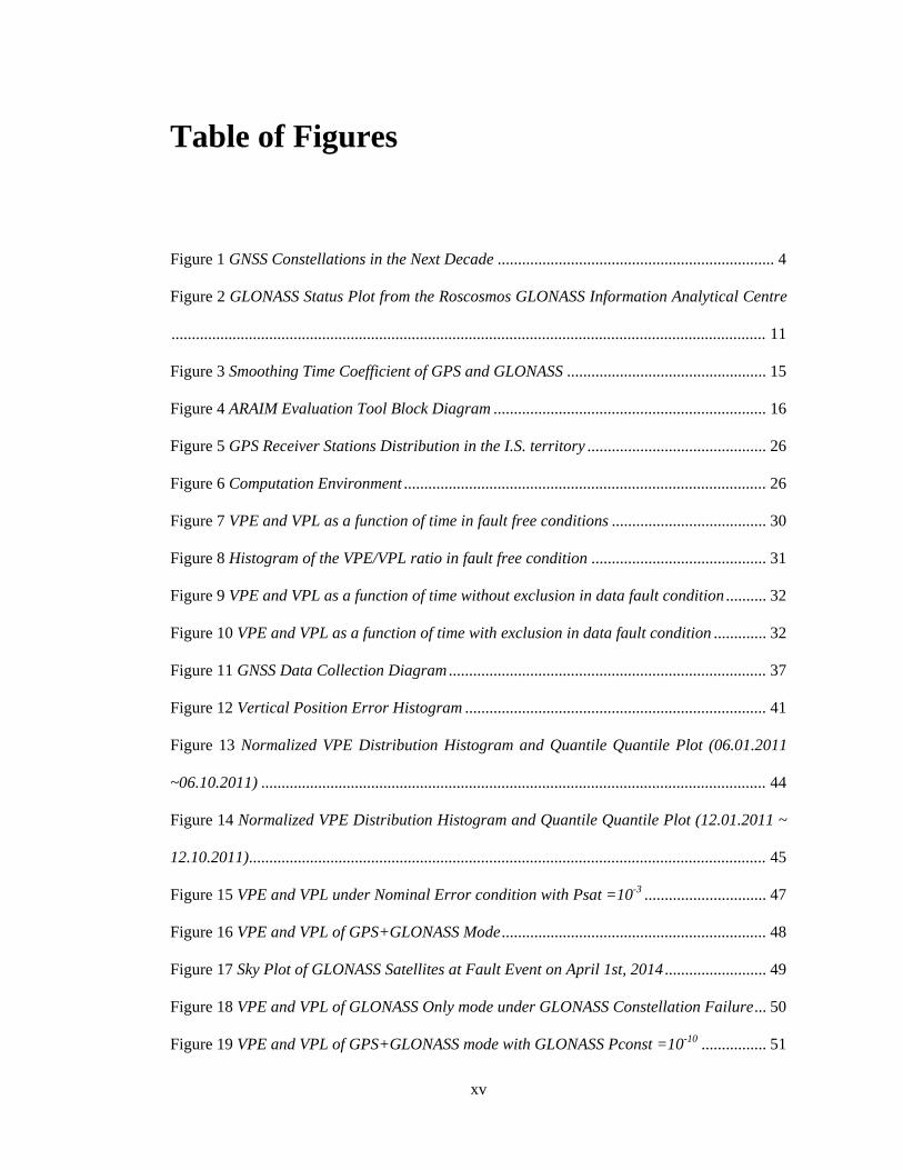
Figure 1 GNSS Constellations in the Next Decade .................................................................... 4

Figure 2 GLONASS Status Plot from the Roscosmos GLONASS Information Analytical Centre

.................................................................................................................................................. 11

Figure 3 Smoothing Time Coefficient of GPS and GLONASS ................................................. 15

Figure 4 ARAIM Evaluation Tool Block Diagram ................................................................... 16

Figure 5 GPS Receiver Stations Distribution in the I.S. territory ............................................ 26

Figure 6 Computation Environment ......................................................................................... 26

Figure 7 VPE and VPL as a function of time in fault free conditions ...................................... 30

Figure 8 Histogram of the VPE/VPL ratio in fault free condition ........................................... 31

Figure 9 VPE and VPL as a function of time without exclusion in data fault condition .......... 32

Figure 10 VPE and VPL as a function of time with exclusion in data fault condition ............. 32

Figure 11 GNSS Data Collection Diagram .............................................................................. 37

Figure 12 Vertical Position Error Histogram .......................................................................... 41

Figure 13 Normalized VPE Distribution Histogram and Quantile Quantile Plot (06.01.2011

~06.10.2011) ............................................................................................................................ 44

Figure 14 Normalized VPE Distribution Histogram and Quantile Quantile Plot (12.01.2011 ~

12.10.2011) ............................................................................................................................... 45

Figure 15 VPE and VPL under Nominal Error condition with Psat =10-3 .............................. 47

Figure 16 VPE and VPL of GPS+GLONASS Mode ................................................................. 48

Figure 17 Sky Plot of GLONASS Satellites at Fault Event on April 1st, 2014 ......................... 49

Figure 18 VPE and VPL of GLONASS Only mode under GLONASS Constellation Failure ... 50

Figure 19 VPE and VPL of GPS+GLONASS mode with GLONASS Pconst =10-10 ................ 51

xvi

Figure 20 VPE and VPL of GPS+GLONASS mode with GLONASS Pconst =10-4 .................. 51

1

Chapter 1 Introduction

1.1 A New Era for the GNSS Environment

The United States' Global Positioning System is the first member of the Global Navigation

Satellite System and is fully operational. While establishing the GPS constellation, the

Russian GLONASS was also launched to build another constellation. Currently, GPS and

GLONASS are fully established and provide navigation to millions of users everywhere on

land, on the ocean surface, and in space. This GNSS environment has faced two significant

changes. These are the modernization plan of the already completed constellations and the

advent of new navigation satellite systems. This section describes these two major

enhancements in the GNSS environment.

1.1.1 Modernization Plan for GPS and GLONASS

The major modernization plan for GPS involves transmitting new civil signals and military

signals. The modernization plan was initiated in the late 1990s. Before 2005, GPS satellite

Blocks II/IIA/IIR transmitted C/A coded signal on the L1 (1575.43 MHz) frequency band and

the P(Y) legacy military code on the L1 and L2 (1227.40 MHz) frequency bands. That is, GPS

satellites transmitted signals for civil users on only one aeronautical frequency, L1. Since the

2

civil application of GPS was becoming important, and the number of users had increased

dramatically, the GPS modernization plan included broadcasting not only new military signals,

but also new civil signals in new frequency bands. Specifically, the civil signal will be

transmitted in three different frequencies. GPS satellite Blocks IIR-M and IIF which broadcast

the new signal scheme have been launched starting in 2005. Specifically, Block IIR-M

satellites are broadcasting a new military signal, M code, on the L1 and L2 frequencies, and a

new civil signal, L2C on L2 in addition to the pre-existing C/A code on L1. The first Block

IIR-M satellite was launched in 2005. It was also planned to broadcast a new civil signal L5 at

a new frequency band centered at 1176.45 MHz. Like the C/A code, this signal is also within

an Aeronautical Radio Navigation Service (ARNS) radio band. This plan was also deployed

for the Block IIF satellites and the first satellite was launched in 2010. In summary, the GPS

constellation will broadcast C/A, L2C, and L5 signals for civil use on L1, L2, and L5

frequencies, respectively, and P(Y) and M code both on L1 and L2 frequencies. It appears that

full modernization plan will be realized sometimes after 2020 [1].

GLONASS became fully operational with 24 satellites in October 2011. The GLONASS

program was inaugurated in the Soviet Union in 1976 and the constellation was established in

1995. Though the peak of 24 healthy satellites was achieved in 1995, the constellation

experienced a painful period of dropping down to 6 operational satellites due to the short life

span of the satellites and several launch failures. Subsequently, Russian Aerospace Defence

Forces restored the system and GLONASS has again reached a steady state with 24 satellites

in 2011. GLONASS also has modernization plans including additional frequency allocation

for a new signal and employing Code-Division Multiple Access (CDMA) rather than

Frequency Domain Multiple Access (FDMA), which is currently used by GLONASS.

GLONASS satellites transmit signals near the L1 frequency band (1598.0625 ~ 1607.0625

MHz) and L2 frequency band (1242.9375 ~ 1249.9375 MHz) using the FDMA scheme. But

3

starting in 2011, the third generation of GLONASS satellites, which is called GLONASS-K, is

transmitting the CDMA signal employed on the newly allocated frequency band (1202.25

MHz). The GLONASS system will transmit CDMA signals in the existing L1 and L2 bands

starting in 2015 [1].

1.1.2 Advent of New Constellations

Since the Global Navigation Satellite System was initiated, starting in the United States with

GPS, other new GNSS constellations including Russian GLONASS, European Galileo,

Chinese Beidou, Japanese Quasi-Zenith Satellite System (QZSS), and the Indian Regional

Navigation Satellite System (IRNSS) are being launched and built to complement each other

[2]. Similar to GPS, Galileo and Beidou are global systems that transmit signals everywhere

on Earth, while QZSS and IRNSS are regional systems that augment other constellations like

GPS.

European Galileo has different business and political models from GPS. Galileo will be

operated based on international participation and investment and produce revenues from

encryption and services. There are multiple services classified into one free service and three

fee based services. Open Service (OS) is free to any users like GPS and used for general

navigation systems such as cellular phone and vehicle navigation systems. In time, Galileo

may offer Commercial Service (CS), Safety-of-Life Service (SoL), and Public Regulated

Service (PRS), which provide higher performance, with additional fees. The Galileo

constellation will consist of 24 satellites and full completion is expected by 2019. Signals will

be transmitted in four frequency bands: E5A, E5B, E6, and E2-L1-E1. These signals fall in

near L1, near L5, and E6 at 1278.75 MHz and they are interoperable with GPS signals. This

interoperation was achieved through considerable negotiation and coordination. Galileo

utilizes CDMA like GPS [1].

4

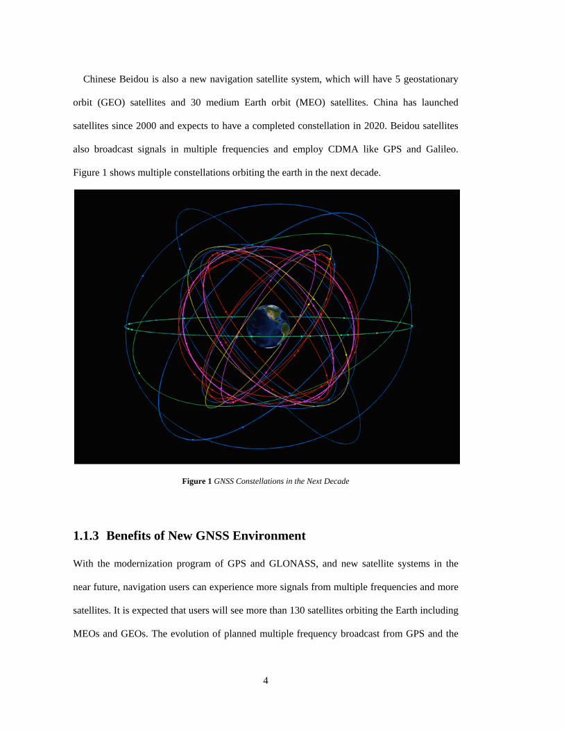
Chinese Beidou is also a new navigation satellite system, which will have 5 geostationary

orbit (GEO) satellites and 30 medium Earth orbit (MEO) satellites. China has launched

satellites since 2000 and expects to have a completed constellation in 2020. Beidou satellites

also broadcast signals in multiple frequencies and employ CDMA like GPS and Galileo.

Figure 1 shows multiple constellations orbiting the earth in the next decade.

Figure 1 GNSS Constellations in the Next Decade

1.1.3 Benefits of New GNSS Environment

With the modernization program of GPS and GLONASS, and new satellite systems in the

near future, navigation users can experience more signals from multiple frequencies and more

satellites. It is expected that users will see more than 130 satellites orbiting the Earth including

MEOs and GEOs. The evolution of planned multiple frequency broadcast from GPS and the

5

other constellations enable users to estimate and cancel the range errors generated as the radio

signal propagates through the ionosphere. Another advantage of multiple frequency diversity

is overcoming the effect of accidental radio frequency interference, resulting in robustness of

service. In addition, since GNSS receivers can see more satellites in view due to the increasing

number of new constellations, the user geometry is stronger, which results in better accuracy

of the position estimate and more redundancy. These two advantages directly improve the

performance of the GNSS navigation system. These parameters are described in [3], [4], [5]

and are given below:

• Accuracy : The GNSS position error is the difference between the estimated position

and the actual position. For an estimated position at a specific location, the probability

should be at least 95% that the position error is within the accuracy requirement.

Accuracy is a multiple of the standard deviation of the position error under nominal

fault free conditions. Accuracy is associated with satellite size and measurement

errors.

• Integrity : Integrity measures the trust that can be placed in the correctness of the

information supplied by the total system. Integrity includes the ability of a system to

provide timely and valid warnings to the user (alerts) when the system must not be

used for the intended operation (or phase of flight). It is represented as integrity risk,

which is the probability that an undetected anomalous signal or satellite fault would

cause Hazardously Misleading Information (HMI). Given that the system integrity is

• valid, the navigation system should produce reliable error bounds on the position

errors under any situation in real time.

• Continuity: Continuity of service of a system is the capability of the system to

perform its function without unscheduled interruptions during the intended operation.

6

Continuity risk is the probability of loss of service or interruption within a given time

period..

• Availability : The availability of a GNSS enabled operation or phase of flight is

characterized by the portion of time during which reliable and sufficient navigation

information is presented to the crew, autopilot, or other system managing the flight of

the aircraft. It is the percentage of time that the system can use the signal from

satellites during the phase of operation. Specifically in this thesis, availability of a

given operation is the time percentage that the accuracy, integrity, and continuity

navigation requirements are met.

1.2 Previous Work

GNSS has supported air navigation for several years, both autonomously (RAIM for

horizontal guidance) and with augmentation (Satellite-based Augmentation Systems, Ground-

based Augmentation Systems, both offering vertical guidance). Navigation systems support

various flight phases including taxi, take-off, climb, en-route flight, approach, and landing.

Approach is one of the most critical phases during flight, and so-called precision approach

provides information for lateral navigation (LNAV) and vertical navigation (VNAV). Lateral

and vertical guidance down to an altitude of 200 feet above ground is called an LPV-200

precision approach procedure (where LPV refers to Localizer Performance with Vertical

Guidance). Lateral guidance during the approach procedure of flight has been supported

through RAIM. Under certain assumptions, RAIM has the ability to detect faulty

measurements at any given time epoch by checking the measurement residuals. Several RAIM

schemes have been proposed [6], [7], [8], [9], [10], [11], [12]. Though many RAIM schemes

had been studied and suggested, the Minimum Operational Performance Standards (MOPS)

7

does not strictly specify any particular RAIM methods. It was left up to the manufacturer to

choose among the various schemes the one that best fits the equipment at hand [10]. For

several years, RAIM has been successfully used for horizontal positioning with protection

levels on the order of several hundreds of meters [13]. However, this traditional RAIM can

only support lateral navigation [14]. Currently, RAIM cannot be used for vertical guidance

because it is based on single frequency and uses only the GPS constellation, and safety

requirements, which will be discussed in Section 1.3, for vertical guidance are tighter than

lateral guidance. Therefore, an extended version of RAIM, called Advanced RAIM (ARAIM),

overcomes the restrictions of traditional RAIM, and satisfies the more stringent integrity

requirements for vertical navigation. The GNSS Evolutionary Architecture Study (GEAS)

report studies development of the ARAIM algorithm [15]. The rationale behind this evolution

can be explained by the following reasons [16]. First, current RAIM is implemented under the

single GPS broadcast frequency at L1, so that it is susceptible to the delay introduced by the

ionosphere, while ARAIM would utilize dual frequency (L1, L5), which enables the

cancellation of the ionospheric delay. Second, ARAIM would use several constellations.

Third,, navigation requirements that assure possible use of ARAIM are stricter than RAIM.

For example, the vertical alert limit (VAL) for the vertical protection level which bounds

vertical position error is 35 meters, while the most stringent operations supported by RAIM

only require a horizontal protection level of about 200 meters. In addition, the integrity

assurance level for LNAV is major (10-5), but the level required for vertical guidance is

severe-major/hazardous (10-7). Fourth, the fault mode assumption for RAIM is that only one

satellite has a failure and additional satellite faults are ignored. On the other hand, multiple

faults including multiple satellite faults and multiple constellation faults should be considered

by ARAIM. Based on the above reasons, RAIM only supports LNAV, while ARAIM would

support vertical guidance of LPV-200. Currently, ARAIM has not yet been standardized and is

8

being currently investigated, so that several ARAIM algorithms have been studied and

proposed to achieve maturity [13], [15], [16], [17], [18], [19], [20], [21], [22]. Due to the

stricter requirements, ARAIM should be scrutinized and evaluated more carefully in order to

give confidence to possible use in vertical guidance. Through extensive validation work, this

thesis pursues the possible use of ARAIM for worldwide coverage of vertical guidance of

aircraft based on more constellations and frequency diversity.

1.3 ARAIM Goals

As stated in [GEAS, WG-C reference], the main purpose of ARAIM is to achieve global

coverage for LPV-200 approach, which provides vertical guidance for aircraft down to 200

feet above the ground, by meeting the corresponding approach requirements. The navigation

requirements for LPV-200 are mainly described in the ICAO Standards and Recommended

Practices (SARPs) [5]. This thesis specifies the requirements in terms of performance metrics

based on related literature [16], [22] and standards [5]. In this section, the performance

requirements for LPV-200 indicated by the corresponding performance metrics are described.

1.3.1 Navigation Requirements

1.3.1.1 Probability of Hazardously Misleading Information (PHMI) is 10-7/ Approach

Integrity is usually measured by the probability of hazardously misleading information

(PHMI). HMI occurs when the Vertical Position Error (VPE) is larger than the Vertical

Protection Level (VPL), guaranteed by the navigation system. PHMI is defined in [23], [24].

For LPV-200, the integrity risk is that PHMI must not exceed 10-7 /approach [16].

(1)

710)Pr( −=<> PHMIVPLVPE

9

1.3.1.2 The Vertical Alert Limit (VAL) is 35 m (Integrity, Availability)

For integrity assurance, the VPE should be less than the VPL and for LPV-200, the VPL must

be below the VAL, which is 35 meters, for 99.99999% of the time during approach operations.

The availability will be measured by the percentage of time that the VPL is less than the VAL

under the condition that the VPL is greater than the VPE given the integrity requirement.

1.3.1.3 Probability of False Alert (Continuity Risk) is 4 × 10-6 per 15 sec (Continuity)

For ARAIM, the airborne algorithm tests have a finite probability of false alert, which can

cause a continuity break [22]. Continuity Risk is the probability of the total continuity budget

allocated to disruptions due to false alert. The allowable false alert probability per sample is

assumed to be the same as the probability per 15 second interval. This probability must be

below 4 × 10-6 [16].

1.3.1.4 Accuracy of the Vertical Position Error (VPE)

While integrity measures the tails of the position error distribution, accuracy measures the

core of the error distribution. Specifically, the 95% accuracy of the VPE shall be 4 meters for

LPV-200 operations. The 99.99999% accuracy of the VPE shall be 10 meters or less. These

quantities are evaluated in the absence of a system failures or rare natural events such as

ionospheric storms.

1.4 Problem Statement

GNSS navigation is susceptible to faults from many origins. For integrity, we are concerned

with the faults that would affect the range errors. Thus, a threat model for ARAIM has been

developed. This threat model associates a priori probabilities to the fault modes, and these

probabilities are used in the airborne algorithm [16], [21]. The list of threats is defined in [21].

Integrity monitoring consists of examining a signal and a navigation message to detect faults

10

and exclude them at any given time. As mentioned in Section 1.2, conventional RAIM

algorithms are currently used for integrity assurance for LNAV approach operations, and were

designed to assure that integrity requirements are met under the assumption that a signal fault

exists on at most a single satellite [16]. Range errors that could cause a hazard for LPV-200

could occur on more than one satellite at the same time. Multiple signal faults have been

observed historically in GLONASS as described in [16]. If the probability of multiple faults is

not taken into account the receiver will not bound the integrity risk. For example, if all range

errors were faulty but consistent within one constellation, the receiver could not detect a fault

using only that constellation. Therefore, ARAIM must have the capability of detecting a fault

under a multiple fault assumption, and a recent ARAIM user algorithm has been proposed in

[22]. In addition, an extensive validation effort on a proposed ARAIM prototype using real

GNSS signals is necessary and is the subject of this thesis.

Moreover, validation of the ARAIM algorithm with real GNSS signals under nominal error

conditions is also not enough to build confidence. Testing the ARAIM algorithm under a

single satellite and multiple satellite assumption with real fault conditions is a very important

part of the validation of ARAIM. It is extremely hard to collect measurements and data of real

fault conditions, because they are unfortunately rare. However, recently, the GLONASS

constellation experienced a fault lasting 11 hours, from just past midnight until noon Russian

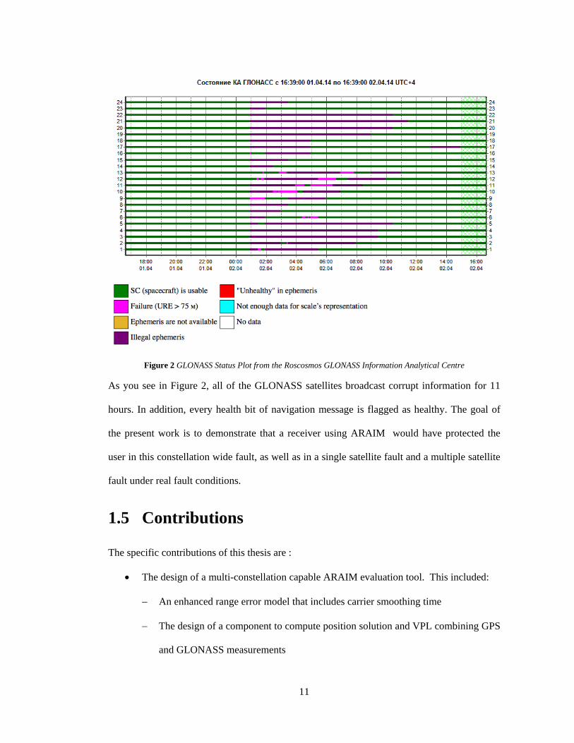
time (UTC+4), on April 2 (or 5 p.m. on April 1 to 4 a.m. April 2, U.S. Eastern time) [25].

11

Figure 2 GLONASS Status Plot from the Roscosmos GLONASS Information Analytical Centre

As you see in Figure 2, all of the GLONASS satellites broadcast corrupt information for 11

hours. In addition, every health bit of navigation message is flagged as healthy. The goal of

the present work is to demonstrate that a receiver using ARAIM would have protected the

user in this constellation wide fault, as well as in a single satellite fault and a multiple satellite

fault under real fault conditions.

1.5 Contributions

The specific contributions of this thesis are :

• The design of a multi-constellation capable ARAIM evaluation tool. This included:

− An enhanced range error model that includes carrier smoothing time

− The design of a component to compute position solution and VPL combining GPS

and GLONASS measurements

12

• The evaluation of an ARAIM algorithm with a large amount of real GPS and

GLONASS signals. This included:

− The testing of the single satellite failure assumption under nominal error

conditions with GPS constellation

− The testing of a multiple satellite failure assumption under nominal error and real

fault conditions with GPS and GLONASS constellations

Through the above tests, this thesis demonstrates that the ARAIM algorithm has the potential

of meeting the requirements for LPV-200 approaches in the near future.

1.6 Outline

This thesis is organized in order of the above-listed contributions.

Chapter 2 explains how to model the range error and how to integrate multi-constellation

measurements in the Multi-Constellation ARAIM user algorithm and evaluation tool.

Chapter 3 presents the data collection, the evaluation method, the evaluation setup, and the

result of ARAIM evaluation under a single satellite fault with a single constellation using GPS.

The evaluation uses the data from 82 reference stations in CONUS and the results are

evaluated under fault free conditions and data fault conditions.

Chapter 4 extends the evaluation of Chapter 3, to multiple fault and multiple constellation.

Specifically, this chapter tests Multi-Constellation ARAIM with GPS and GLONASS and

considers all the navigation requirements discussed above. The evaluation is executed in three

different kinds of constellation combinations, which are GPS only, GLONASS only, and GPS

plus GLONASS. The ARAIM algorithm used to evaluate the VPL bounding performance

under multiple satellite failures and the constellation failure assumption.

Chapter 5 summarizes the methods and the results of the evaluation, and provides several

ideas for possible future work.

13

Chapter 2 Multi-Constellation ARAIM user Algorithm

2.1 Nominal Range Error Model

The range error model is a key input of the ARAIM algorithm and therefore an important role

in this work. In addition to predicting accuracy, the nominal error model determines in large

part the strength of the integrity monitoring. In this section, the nominal range error model will

be described. The nominal error model includes conditions that are always present: nominal

clock and ephemeris, tropospheric error, code noise, and multipath [21]. Since the nominal

error model is used to compute the position error and the protection level, it must be

accurately characterized and bounded. As noted in [19], the ARAIM algorithm will be

implemented in an airborne situation. Hence, we used the error model of an airborne receiver,

even though we collected real data through a ground receiver. We call that nominal error

model Airborne Accuracy Designators (AAD-A). For each pseudorange, the error is

characterized by a Gaussian distribution. The total range error is the sum of all the error

components mentioned above and these can be treated as independent random variables. The

total variance of the nominal pseudorange error is the sum of variances of URA, tropospheric

delay, and code noise and multipath (CNMP) error and it is given by:

(2) 2_,

2,

2,

2airDFktropokURAkk σσσσ ++=

14

where the tropospheric error is defined as:

(3)

The CNMP error corresponding to an iono-free combination is given by:

(4)

(5)

The noise term is specified as:

(6)

where is the th satellite measurement, is elevation angle, and , are the L1

and L2 frequencies. Since the ionospheric delay is removed from the linear combination of

dual frequency measurements, we do not have to consider the ionospheric delay. One of the

largest components of the overall nominal error is the multipath error. In this work, it is

modeled as a function of carrier smoothing time as well as elevation angle. If the smoothing

time is short, the multipath error is larger than the error with a longer smoothing time. So we

characterized the multipath variance equation applying the coefficient given by:

(7)

The multiplication factor is the smoothing time coefficient and it is given by the

following:

( )( ), 2

1.0010.120.002001 sin

k tropo

k

mEl

σ = ⋅ +

2,,22

22

1

222

,,122

21

212

_, airkLairkLairDFk fff

fff σσσ

−

+

−

=

2,

2,

2,,2

2,,1 multipathknoisekairkLairkL σσσσ +==

( )( ) ( ), 0.04 0.02 5 / 85k noise km mσ θ= − − ° °

k k kθ 1Lf 2Lf

)53.013.0( 10/,

keCstmultipathk

θσ −×+×=

stC

15

(8)

where is the converging time for the respective constellation and , are the coefficient

curve constants for the constellation, respectively.

The coefficient is inversely proportional to the square root of smoothing time and

converges to one at a given time . Initially, we treated this smoothing time coefficient

equally for both GPS and GLONASS by using the same parameters. But it turned out that the

accuracy of GPS+GLONASS was worse than that of GPS alone, which means that we were

not applying the correct weights when forming the position solution. We could infer from the

previous result that we had to increase the values of and for GLONASS, and adjust the

ones for GPS as well. In other words, we need to place much more weight on GPS rather than

GLONASS. The resulting curve is shown in Figure 3.

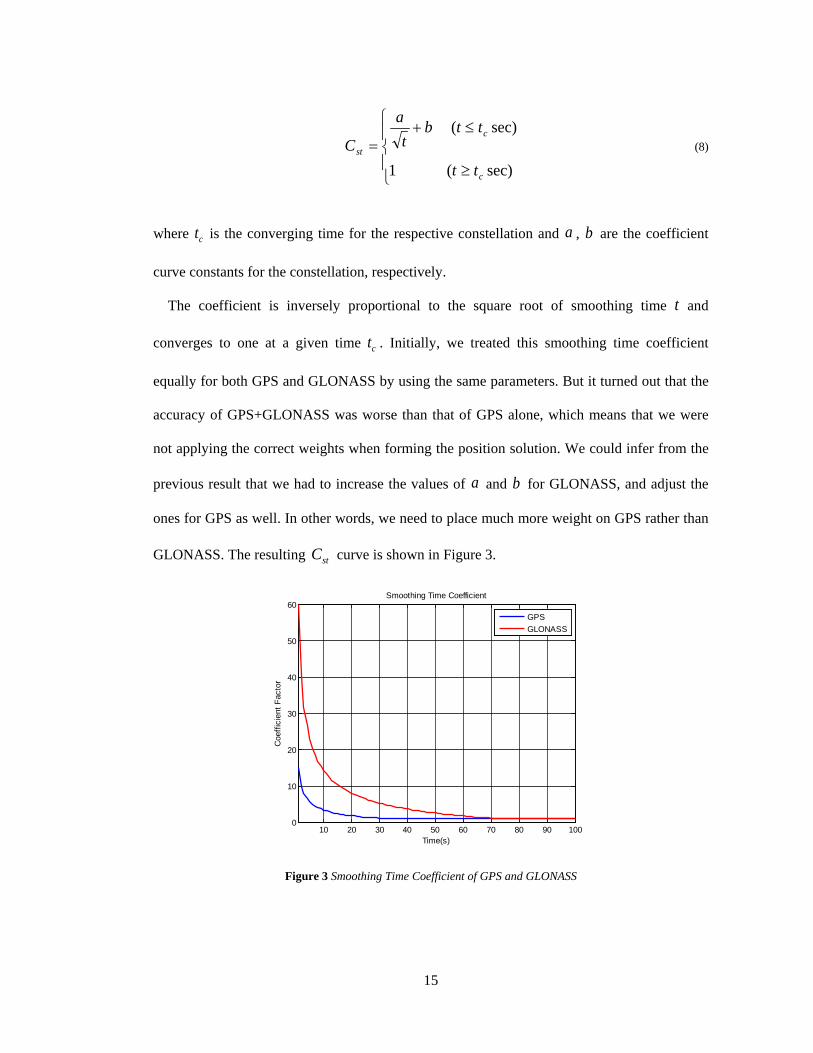
Figure 3 Smoothing Time Coefficient of GPS and GLONASS

≥

≤+=

sec)(1

sec)(

c

c

st

tt

ttbt

a

C

ct a b

t

ct

a b

stC

10 20 30 40 50 60 70 80 90 1000

10

20

30

40

50

60

Time(s)

Coe

ffici

ent F

acto

r

Smoothing Time Coefficient

GPSGLONASS

16

The models shown in Figure 3 were determined by a trial and error scheme, by examining

the statistics of the position error divided by the predicted accuracy, as shown in the next

section. Figure 3 shows that the initial multiplication factor of GLONASS is far greater than

that of GPS and the converging time of GLONASS is longer than that of GPS as well. The

GLONASS smoothing time coefficient starts from 60 and converges to 1 at 70 s. The GPS

curve initiates at the value of 15 and converges at 30 s.

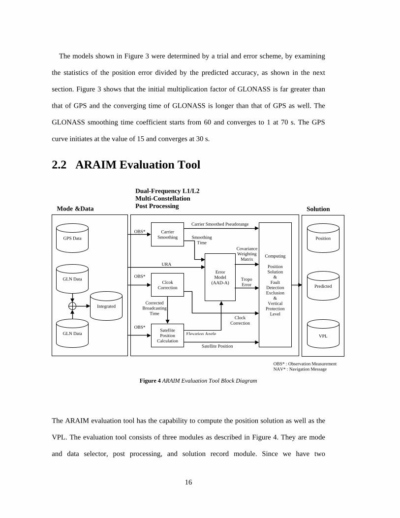
2.2 ARAIM Evaluation Tool

The ARAIM evaluation tool has the capability to compute the position solution as well as the

VPL. The evaluation tool consists of three modules as described in Figure 4. They are mode

and data selector, post processing, and solution record module. Since we have two

Mode &Data

Dual-Frequency L1/L2 Multi-Constellation Post Processing

Solution

Position

Predicted

VPL

GPS Data

Integrated

GLN Data

GLN Data

Error Model

(AAD-A)

Computing

Position Solution

& Fault

Detection Exclusion

& Vertical

Protection Level

OBS*

OBS*

OBS*

Carrier Smoothing

Clcok Correction

Satellite Position

Calculation

Smoothing Time

Carrier Smoothed Pseudorange

Corrected Broadcasting

Time

Elevation Angle

Satellite Position

Clock Correction

Covariance Weighting

Matrix URA

Tropo Error

OBS* : Observation Measurement NAV* : Navigation Message

Figure 4 ARAIM Evaluation Tool Block Diagram

17

constellations’ worth of data, three combination modes can be chosen by users, which are GPS

only, GLONASS only, or integrated GPS and GLONASS mode. If the mode is selected by the

user, the data management component loads the available data set and distributes it to the post

processing module. With the navigation messages and the observation measurements, satellite

clock biases and satellite positions are computed in the corresponding component, respectively.

Carrier smoothing is also implemented for the next process which is position computing. In

this component, ionosphere-free combinations are used for both code and carrier inputs to the

smoothing filter in order to remove ionospheric delay. In addition, the carrier smoothing

component not only sets the smoothing time filter to 200 s, but also records each satellite

measurement’s smoothing time in order to characterize the range error model. Then, the

outputs, satellite elevation angle and smoothing time from previous components and the URA,

which is one of the elements in the navigation message, are transferred into the error model

component. In the error model component, the total variance that contains multipath, receiver

noise, and tropospheric error model is calculated to produce the weighting matrix for the

weighted least square solution in position computing. Finally, the ARAIM tool calculates the

position solution. After that, it checks to see if the measurement residuals are consistent. If

they are not, it attempts to exclude the measurement causing the inconsistency (and most

likely faulted. If the fault detection test is passed as described in [26], the tool computes the

VPL. Lastly, if the process is over, the solution record module saves all the resulting data.

2.2.1 GLONASS only mode

Since the GLONASS satellite transmits different navigation messages from GPS, GLONASS

has another scheme to calculate satellite clock bias and satellite position based on GLONASS

ICD [27]. Also several considerations are required to get a position solution using GLONASS

signals. First, since each GLONASS satellite transmits a signal with a respective carrier

18

frequency, the available frequency value should be reflected in the computation of the error

model, such as Equation (4), and carrier smoothing as described in Table 1. Next, considering

Earth’s rotation rate and the time difference between the instant in time of signal reception and

the time of signal transmission, there was a common bias term in the east component of the

position error. Because the factor that causes common bias could not be determined even after

careful analysis, we characterized the bias term in the position domain and tracked back errors

in the range domain. We then subtracted range domain errors from the measurements and

computed the position solution again. Other issues such as time scale and reference coordinate

system will be presented in the following paragraph.

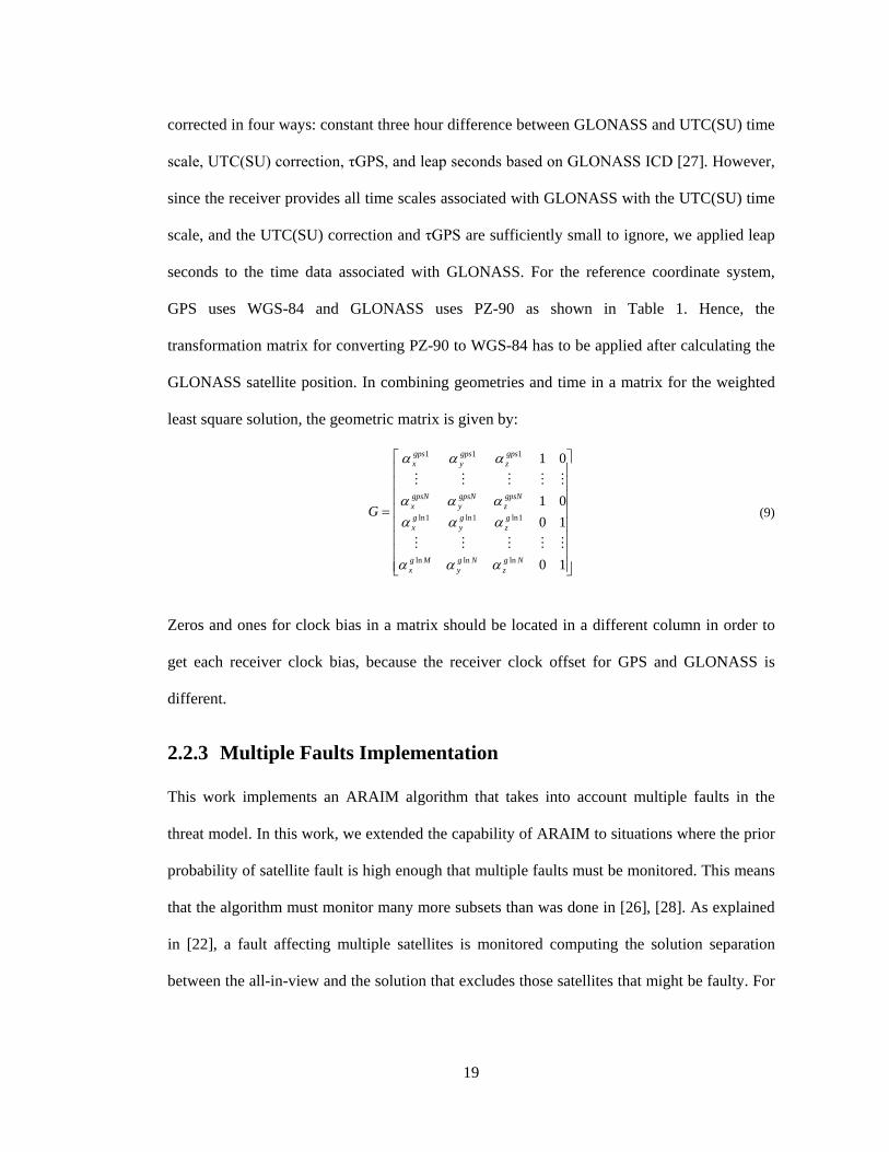
Table 1 Comparison of GPS and GLONASS

Parameter GPS GLONASS Time Scale UTC(USNO) UTC(SU) Reference Coordinate WGS-84 PZ-90

Carrier Frequency

L1:1602.0+0.5625k L2:1246.9+0.4375k

k = 0,1…12

L1:1575.42 L2:1227.6

Ephemeris Keplerian elements

Rectangular Coordinates

2.2.2 Combining GPS and GLONASS

One of the key features in this paper is to compare the performance between single

constellation mode and multi-constellation mode. As a result, in integrated GPS and

GLONASS mode, the different reference parameters should be synchronized with one

reference frame for exact comparison. Table 1 presents key parameters that should be

considered in combining GPS and GLONASS signals. In this work, since every signal is

measured based on the GPS time standard in the receiver, all the reference parameters were

matched up with GPS. Thus, for time scale, originally GLONASS time should have been

19

corrected in four ways: constant three hour difference between GLONASS and UTC(SU) time

scale, UTC(SU) correction, τGPS, and leap seconds based on GLONASS ICD [27]. However,

since the receiver provides all time scales associated with GLONASS with the UTC(SU) time

scale, and the UTC(SU) correction and τGPS are sufficiently small to ignore, we applied leap

seconds to the time data associated with GLONASS. For the reference coordinate system,

GPS uses WGS-84 and GLONASS uses PZ-90 as shown in Table 1. Hence, the

transformation matrix for converting PZ-90 to WGS-84 has to be applied after calculating the

GLONASS satellite position. In combining geometries and time in a matrix for the weighted

least square solution, the geometric matrix is given by:

(9)

Zeros and ones for clock bias in a matrix should be located in a different column in order to

get each receiver clock bias, because the receiver clock offset for GPS and GLONASS is

different.

2.2.3 Multiple Faults Implementation

This work implements an ARAIM algorithm that takes into account multiple faults in the

threat model. In this work, we extended the capability of ARAIM to situations where the prior

probability of satellite fault is high enough that multiple faults must be monitored. This means

that the algorithm must monitor many more subsets than was done in [26], [28]. As explained

in [22], a fault affecting multiple satellites is monitored computing the solution separation

between the all-in-view and the solution that excludes those satellites that might be faulty. For

=

10

1001

01

lnlnln

1ln1ln1ln

111

Ngz

Ngy

Mgx

gz

gy

gx

gpsNz

gpsNy

gpsNx

gpsz

gpsy

gpsx

G

ααα

αααααα

ααα

20

example, with a prior probability of 10-5 and 10 satellites, the probability of having two or

more simultaneous faults is less than :

Since this is smaller than the integrity budget specified in [22], the algorithm does not need to

check multiple faults. However, if the prior probability is 10-4 , then the probability becomes:

which exceeds the integrity budget. This means that the algorithm must check all the subsets

of two satellites (because the probability of having more than three is less than the integrity

budget). In real time, the ARAIM algorithm generates subsets which exclude simultaneous

faulty satellites in the set and the number of simultaneous faulty satellites ranges from 1 to n ,

where n is the given number of satellites. However, we do not have to monitor all subsets (of

which there are 2n). Instead, we used a probability threshold for the integrity risk coming from

unmonitored satellite faults. Based on this probability threshold and prior probability, the

algorithm determines the total number of subsets that need to be monitored, so that the

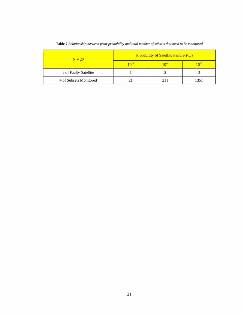
algorithm does not consume unnecessary computation time. Given 20 satellites, Table 2 gives

an example of the relationship between probability of satellite fault and number of subsets that

require monitoring. If prior probability Psat is 10-5, with constraint level of safety of 10-7 , then

we had to account for the possibility that there is one satellite failure. The corresponding

number of subsets that require monitoring by the ARAIM algorithm is therefore 21. As prior

probability increases, the number of simultaneous faulty satellites and subsets monitored also

increases. As the number of subsets becomes greater, the real time vertical protection level

will increase. Thus, we can say that the vertical protection level is a function of the probability

of satellite failure. For a more detailed description of the multiple faults implementation, the

reader may refer to [22].

( )25 91010 4.5 10

2− −

= ×

( )24 71010 4.5 10

2− −

= ×

21

Table 2 Relationship between prior probability and total number of subsets that need to be monitored

N = 20 Probability of Satellite Failure(Psat)

10-5 10-4 10-3

# of Faulty Satellite 1 2 3

# of Subsets Monitored 21 211 1351

22

23

Chapter 3 ARAIM Evaluation with a Single

Constellation (GPS)

This chapter presents the process and outcomes of the ARAIM algorithm prototype using dual

frequency measurements acquired from ground GPS receiver stations. The purpose of the test

of this chapter is to verify the ARAIM algorithm prototype which was proposed in [13], [16].

In this chapter, the ARAIM algorithm will be evaluated under a single satellite failure

assumption with a single constellation, i.e. GPS. This is the first step for further investigation

of multi-constellation ARAIM, and a test of the enhanced version of the conventional RAIM

algorithm.

This chapter is organized as follows. Section 3.1 explains how to acquire data and the

processing setup for algorithm evaluation. This presents the size, type, period of data, and the

computation methodology. A few assumptions and considerations for the algorithm follow. In

order to produce good performance from the given situation and real data, the multi-path error

model and threat model assumed in previous work [13], [16], [17], [18], [26] are defined.

Moreover, to compute the position solution, the conditions for choosing measurements and the

carrier smoothing method will be presented. The fault detection methodology is illustrated

briefly at the end of the section.

24

In Section 3.2, the results of validation under two types of conditions will be shown. The

analysis of the results shows the robustness of the algorithm. Furthermore, an abnormal case

which was derived during processing will be analyzed.

3.1 ARAIM Evaluation Setup

This section represents the process and outcomes of the ARAIM algorithm prototype using

dual frequency measurements acquired from ground GPS receiver stations. The purpose of

this section is to illustrate the processing setup of data and algorithm.

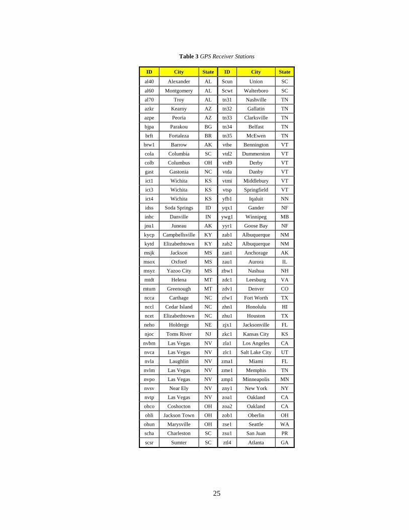
3.1.1 Data Collection

The data was collected from eighty two Continuously Operating Reference Station (CORS)

networks for four months (9/1/2010 – 12/31/2010) in the U.S. territory and worldwide as seen

in Table 3 and Figure 5. The type of data file is RINEX. For dual frequency operations, L1

C/A and L2C semi-codeless code and carrier phase measurements were used. Actually, L5

signals of GPS should be used for dual frequency operation, since the L5 signal is designed

for civil use. As the L5 signal is not yet fully operational, this work used signals on L1 and L2.

L1 C/A and L2C semi-codeless code and carrier phase measurements were sampled at 1 Hz

with a total of 9,461 data files. Each data file has real measurements for twenty four hours for

one receiver station.

25

Table 3 GPS Receiver Stations

ID City State ID City State

al40 Alexander AL Scun Union SC

al60 Montgomery AL Scwt Walterboro SC

al70 Troy AL tn31 Nashville TN

azkr Kearny AZ tn32 Gallatin TN

azpe Peoria AZ tn33 Clarksville TN

bjpa Parakou BG tn34 Belfast TN

brft Fortaleza BR tn35 McEwen TN

brw1 Barrow AK vtbe Bennington VT

cola Columbia SC vtd2 Dummerston VT

colb Columbus OH vtd9 Derby VT

gast Gastonia NC vtda Danby VT

ict1 Wichita KS vtmi Middlebury VT

ict3 Wichita KS vtsp Springfield VT

ict4 Wichita KS yfb1 Iqaluit NN

idss Soda Springs ID yqx1 Gander NF

inhc Danville IN ywg1 Winnipeg MB

jnu1 Juneau AK yyr1 Goose Bay NF

kycp Campbellsville KY zab1 Albuquerque NM

kytd Elizabethtown KY zab2 Albuquerque NM

msjk Jackson MS zan1 Anchorage AK

msox Oxford MS zau1 Aurora IL

msyz Yazoo City MS zbw1 Nashua NH

mtdt Helena MT zdc1 Leesburg VA

mtum Greenough MT zdv1 Denver CO

ncca Carthage NC zfw1 Fort Worth TX

nccl Cedar Island NC zhn1 Honolulu HI

ncet Elizabethtown NC zhu1 Houston TX

neho Holdrege NE zjx1 Jacksonville FL

njoc Toms River NJ zkc1 Kansas City KS

nvbm Las Vegas NV zla1 Los Angeles CA

nvca Las Vegas NV zlc1 Salt Lake City UT

nvla Laughlin NV zma1 Miami FL

nvlm Las Vegas NV zme1 Memphis TN

nvpo Las Vegas NV zmp1 Minneapolis MN

nvsv Near Ely NV zny1 New York NY

nvtp Las Vegas NV zoa1 Oakland CA

ohco Coshocton OH zoa2 Oakland CA

ohli Jackson Town OH zob1 Oberlin OH

ohun Marysville OH zse1 Seattle WA

scha Charleston SC zsu1 San Juan PR

scsr Sumter SC ztl4 Atlanta GA

26

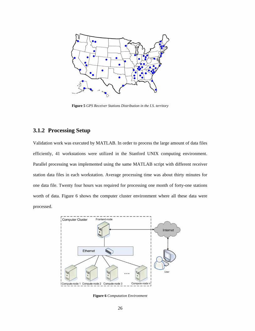
Figure 5 GPS Receiver Stations Distribution in the I.S. territory

3.1.2 Processing Setup

Validation work was executed by MATLAB. In order to process the large amount of data files

efficiently, 41 workstations were utilized in the Stanford UNIX computing environment.

Parallel processing was implemented using the same MATLAB script with different receiver

station data files in each workstation. Average processing time was about thirty minutes for

one data file. Twenty four hours was required for processing one month of forty-one stations

worth of data. Figure 6 shows the computer cluster environment where all these data were

processed.

Figure 6 Computation Environment

27

3.1.3 Algorithm Setup

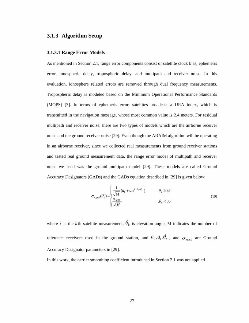
3.1.3.1 Range Error Models

As mentioned in Section 2.1, range error components consist of satellite clock bias, ephemeris

error, ionospheric delay, tropospheric delay, and multipath and receiver noise. In this

evaluation, ionosphere related errors are removed through dual frequency measurements.

Tropospheric delay is modeled based on the Minimum Operational Performance Standards

(MOPS) [3]. In terms of ephemeris error, satellites broadcast a URA index, which is

transmitted in the navigation message, whose most common value is 2.4 meters. For residual

multipath and receiver noise, there are two types of models which are the airborne receiver

noise and the ground receiver noise [29]. Even though the ARAIM algorithm will be operating

in an airborne receiver, since we collected real measurements from ground receiver stations

and tested real ground measurement data, the range error model of multipath and receiver

noise we used was the ground multipath model [29]. These models are called Ground

Accuracy Designators (GADs) and the GADs equation described in [29] is given below:

(10)

where is the th satellite measurement, is elevation angle, M indicates the number of

reference receivers used in the ground station, and , and are Ground

Accuracy Designator parameters in [29].

In this work, the carrier smoothing coefficient introduced in Section 2.1 was not applied.

<

≥+=

−

35,

35,)(1

)(

)/(10

,

kMAX

k

kgndk

M

eaaM

ck

θσ

θθσ

θθ

k k kθ

caa θ,, 10 MAXσ

28

3.1.3.2 Position Solution

With the dual frequency ionosphere free smoothing method, we removed all ionosphere-

related errors using the carrier phase measurements. The carrier smoothing time was set at 100

s which is the maximum filter length. Since the ARAIM assumed that the computation was

executed by receiver alone without any assistance from an augmentation system, we did not

apply differential corrections for the position calculation. The measurements that have Signal

to Noise Ratio (SNR) greater than 25 dB were used for calculations. The mask elevation angle

was 5 degrees and measurements that were from satellites above 5 degrees were used for

computation. The filter is re-initialized after a cycle slip.

3.1.3.3 Fault Detection and Exclusion, VPL Computation (ARAIM)

The ARAIM algorithm implemented in this study is presented in [16]. As in [16], the required

Probability of Hazardously Misleading Information (PHMI) is 10-7 and the Prior Probability

(Psat) which is the probability of satellite fault is 10-5. The continuity risk is 4 × 10-6. We

applied mode one threat model, which assumes there is only one faulty satellite among

satellites in view at any given time. Hence, the algorithm computes the all in view position

solution and subset position solutions, which are position solutions of each subset of size N-1,

where N is the number of satellites in view at any given time. For fault detection, the

algorithm implements a consistency check which includes the solution separations and the chi-

square test [12]. After the position solutions, the algorithm computes the position solution

separation statistics and conducted the solution separation threshold test in order to detect a

faulty satellite [22]. If the test fails, exclusion is attempted. Then the algorithm calculates the

chi-square statistics of each subset solution for sanity check defined as the Weighted Sum of

the Squared Errors (WSSE) such that:

29

(11)

(12)

where G is the observation matrix, W is weighting matrix, and y is an N dimensional vector

containing the raw pseudorange measurements minus the expected ranging values based on

the location of the satellites and the location of the user [12]. The chi-square statistic is only

used to find the outlier in case the solution separation tests were not passed. If the

measurements were deemed consistent the algorithm computes the VPL using the approach

presented in [13]. If the measurements are not consistent, the algorithm excludes the

measurement of faulty satellite in order to verify the consistency of the measurements

excluding the faulty satellite. If the measurements are still inconsistent after exclusion, then

the algorithm sets the VPL to infinity; if not, it computes the VPL as mentioned above. If

there are only four measurements in view at any given time, the algorithm does not compute

the position fix and the VPL.

3.2 ARAIM Evaluation Results

This section demonstrates the validation results for the ARAIM algorithm under two

conditions: the fault free condition, and the data fault condition which is similar to the real

fault condition.

3.2.1 Behavior under Nominal (fault free) Conditions

Under nominal conditions, no HMI event in which the VPE is above the VPL is expected.

After processing all 9461 data files, the validation can be presented by the VPL bounding

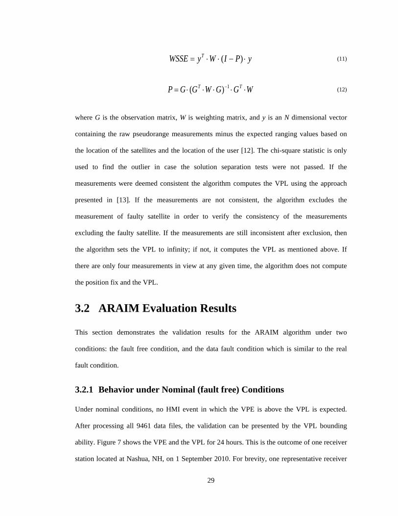
ability. Figure 7 shows the VPE and the VPL for 24 hours. This is the outcome of one receiver

station located at Nashua, NH, on 1 September 2010. For brevity, one representative receiver

yPIWyWSSE T ⋅−⋅⋅= )(

WGGWGGP TT ⋅⋅⋅⋅⋅= −1)(

30

station result is demonstrated in this thesis. The standard deviation of the station is 2.75 meters.

Figure 7 is the visualization of VPL bounding as a series of snapshots for some interval of

time.

Figure 7 VPE and VPL as a function of time in fault free conditions

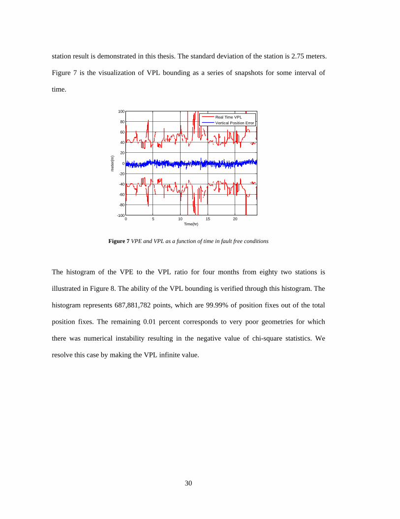
The histogram of the VPE to the VPL ratio for four months from eighty two stations is

illustrated in Figure 8. The ability of the VPL bounding is verified through this histogram. The

histogram represents 687,881,782 points, which are 99.99% of position fixes out of the total

position fixes. The remaining 0.01 percent corresponds to very poor geometries for which

there was numerical instability resulting in the negative value of chi-square statistics. We

resolve this case by making the VPL infinite value.

0 5 10 15 20-100

-80

-60

-40

-20

0

20

40

60

80

100

Time(hr)

met

er(m

)

Real Time VPLVertical Position Error

31

Figure 8 Histogram of the VPE/VPL ratio in fault free condition

3.2.2 Behavior under Data Fault Condition

Over 4 months and 82 receiver stations, we could not find a real fault situation that would

enable the ARAIM algorithm to respond showing the ability of the algorithm. In this

paragraph, we show the ability of ARAIM for fault detection and exclusion under the data

fault condition which is similar to the real fault condition. The reason why it is called the data

fault is that the quality of the RINEX file is not always good. This is not due to the fact that

the measurement itself has fault, but the data have faults that can be derived from data

collecting, also called data assembly. Because of this feature, we could observe a fault

situation similar to a real fault condition. In this case, we first recorded an occurrence of

exclusion and which station conducted exclusion in order to compare outputs between the

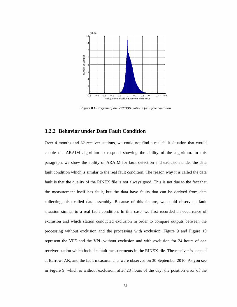
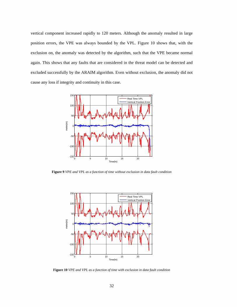
processing without exclusion and the processing with exclusion. Figure 9 and Figure 10

represent the VPE and the VPL without exclusion and with exclusion for 24 hours of one

receiver station which includes fault measurements in the RINEX file. The receiver is located

at Barrow, AK, and the fault measurements were observed on 30 September 2010. As you see

in Figure 9, which is without exclusion, after 23 hours of the day, the position error of the

-0.5 -0.4 -0.3 -0.2 -0.1 0 0.1 0.2 0.3 0.4 0.50

2

4

6

8

10

12

14

16x 10

6

Ratio(Vertical Position Error/Real Time VPL)

Num

ber o

f Sam

ples

million

32

vertical component increased rapidly to 120 meters. Although the anomaly resulted in large

position errors, the VPE was always bounded by the VPL. Figure 10 shows that, with the

exclusion on, the anomaly was detected by the algorithm, such that the VPE became normal

again. This shows that any faults that are considered in the threat model can be detected and

excluded successfully by the ARAIM algorithm. Even without exclusion, the anomaly did not

cause any loss if integrity and continuity in this case.

Figure 9 VPE and VPL as a function of time without exclusion in data fault condition

Figure 10 VPE and VPL as a function of time with exclusion in data fault condition

0 5 10 15 20-150

-100

-50

0

50

100

150

Time(hr)

met

er(m

)

Real Time VPLVertical Position Error

0 5 10 15 20-150

-100

-50

0

50

100

150

Time(hr)

met

er(m

)

Real Time VPLVertical Position Error

33

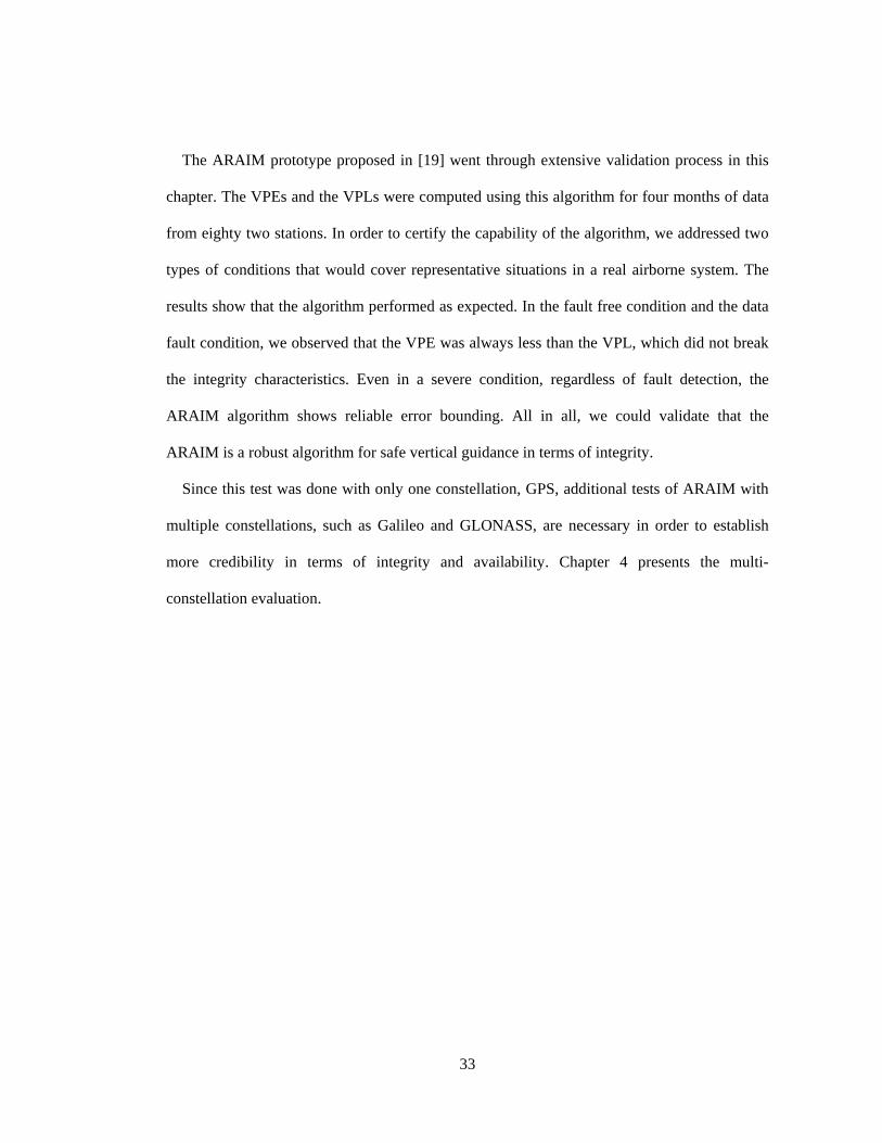
The ARAIM prototype proposed in [19] went through extensive validation process in this

chapter. The VPEs and the VPLs were computed using this algorithm for four months of data

from eighty two stations. In order to certify the capability of the algorithm, we addressed two

types of conditions that would cover representative situations in a real airborne system. The

results show that the algorithm performed as expected. In the fault free condition and the data

fault condition, we observed that the VPE was always less than the VPL, which did not break

the integrity characteristics. Even in a severe condition, regardless of fault detection, the

ARAIM algorithm shows reliable error bounding. All in all, we could validate that the

ARAIM is a robust algorithm for safe vertical guidance in terms of integrity.

Since this test was done with only one constellation, GPS, additional tests of ARAIM with

multiple constellations, such as Galileo and GLONASS, are necessary in order to establish

more credibility in terms of integrity and availability. Chapter 4 presents the multi-

constellation evaluation.

34

35

Chapter 4 ARAIM Evaluation with Multi-

Constellation (GPS+GLONASS)

In Section 3.2, a demonstration using extensive GPS real ground data showed the ability of

ARAIM to effectively bound the VPE. The purposes of this chapter are to extend the work of

Chapter 3 to a multi-constellation setting by using GPS and GLONASS real data, and to verify

the ability of the enhanced version of the ARAIM algorithm proposed in [22]. This will

present one of the first demonstrations of multi-constellation ARAIM with GPS and

GLONASS real data. This chapter is presented as follows. First, the data collection details and

algorithm setup are presented in Section 4.1. This explains how the GPS and GLONASS real

measurement data and navigation messages were obtained from the receiver, and how they

were processed. Then, the ARAIM evaluation setup is described including multipath error

model, fault detection, and exclusion scheme.

In Section 4.2, the evaluation of the algorithm will be presented and it will be customized to

the navigation requirements, such as accuracy, integrity, continuity, and availability. It is also

demonstrated in three different modes, which are GPS only mode, GLONASS only mode, and

GPS + GLONASS mode in order to show the benefit of multi-constellation. The evaluation

results are classified in three categories. The first part verifies whether the nominal error

36

models are correct. We do this by evaluating whether predicted position accuracy is well fitted

to the actual position solution accuracy. Then, the VPL bounding performance is analyzed

under nominal error conditions to demonstrate the ability of ARAIM concerning integrity,

continuity, and availability. Additionally, the association of prior probability with VPL value

will be analyzed. Finally, the performance of the ARAIM algorithm will be shown under a

real constellation fault situation.

4.1 ARAIM Evaluation Setup

This section describes the source of the data and the multi-constellation ARAIM algorithm

processing.

4.1.1 Data Collection

The real navigation and measurement data were obtained from a Trimble receiver with

multiple constellation tracking capability. The receiver antenna is on the roof of the Stanford

GPS laboratory. Since the receiver was installed, we have stored all navigation messages and

measurement data that can be tracked by the receiver. Since the receiver can be connected via

TCP/IP, we are able to monitor the satellite tracking and log the stored data in real time. When

the receiver gets the data, it saves it as a *.T02 file format. Users can then access the data on

the intranet. However, the storage volume is not enough to save all the data for several months,

so we established a system that transmits the data into the server computer in the laboratory.

The *.T02 file format is a collective satellite data file format which is comprised of GPS,

GLONASS, Galileo, and WAAS data. Hence it is necessary to convert it into the respective

RINEX file which is a more convenient file format for post processing. With the conversion

tool, we can convert the *.T02 file into a GPS or GLONASS RINEX file. In addition, it is also

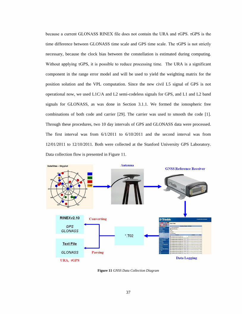
necessary to parse the *.T02 file into a text file extracting the GLONASS navigation message,

37

because a current GLONASS RINEX file does not contain the URA and τGPS. τGPS is the

time difference between GLONASS time scale and GPS time scale. The τGPS is not strictly

necessary, because the clock bias between the constellation is estimated during computing.

Without applying τGPS, it is possible to reduce processing time. The URA is a significant

component in the range error model and will be used to yield the weighting matrix for the

position solution and the VPL computation. Since the new civil L5 signal of GPS is not

operational now, we used L1C/A and L2 semi-codeless signals for GPS, and L1 and L2 band

signals for GLONASS, as was done in Section 3.1.1. We formed the ionospheric free

combinations of both code and carrier [29]. The carrier was used to smooth the code [1].

Through these procedures, two 10 day intervals of GPS and GLONASS data were processed.

The first interval was from 6/1/2011 to 6/10/2011 and the second interval was from

12/01/2011 to 12/10/2011. Both were collected at the Stanford University GPS Laboratory.

Data collection flow is presented in Figure 11.

Figure 11 GNSS Data Collection Diagram

38

In addition, as mentioned in Section 1.4, the data which were affected by the GLONASS

event on April 1st and 2nd were recorded in our receiver. The GLONASS down event was

processed as the most optimal candidate to verify the multi-constellation ARAIM algorithm

and analysis results from those days will be presented in Section 4.2.

4.1.2 Algorithm Setup

4.1.2.1 Range Error Models

Most of the range error components' models are the same as in Section 3.1.3.1. However,

multipath and receiver noise is unlike the previous evaluation in Chapter 3. In this evaluation,

even though the receiver antenna is located on the roof of the four story building, the airborne

receiver noise model was used because the ARAIM algorithm will be implemented in an

airborne situation. We call this nominal error model Airborne Accuracy Designators (AADs)

and the corresponding equation is described in [29] and Section 2.1. Specifically, we used the

adjusted multipath error model as Equation (7) in Section 2.1. By applying the enhanced

multipath error model, we tried to generate well estimated predicted accuracy. In Section 4.2,

the accuracy results will show how well the enhanced multipath error model improves the

positioning performance.

4.1.2.2 Fault Detection and Exclusion, VPL Computation (ARAIM)

Since the purpose of this chapter is multi-constellation processing, the ARAIM algorithm

implemented in this chapter is represented in [22]. All the constants for integrity and

continuity requirements are given in [22] and those values are the same as previous work in

Chapter 3. The required Probability of Hazardously Misleading Information (PHMI) is 10-7

and the continuity risk is 4 × 10-6. The Prior Probability (Psat) which is probability of satellite

fault and the prior probability of constellation fault will be different based on constellation and

39

test purpose to study the relationship between the VPL and the prior probability of satellite

and constellation, respectively. Exact values of prior probabilities will be chosen in Section

4.2. In this chapter, the ARAIM algorithm was tested under a threat model that includes

simultaneous satellite faults. Specifically, the algorithm assumes there is more than one faulty

satellite including a whole constellation fault at any given time. As described in Chapter 2, the

algorithm determines the faults that need to be monitored with given prior probabilities.

Specifically, instead generating only subsets of size N or N-1, the algorithm computes the

maximum size of the subsets that need to be monitored. Note that in determining subsets to be

monitored, subsets with respect to satellite and constellation are considered independently

using the prior probability of satellite and the prior probability of constellation respectively. If

you need more clarification for determining subset size, refer to [22]. Once the subsets to be

monitored are formed, the algorithm calculates all in view position and separate subset

solutions as was done in Chapter 3. For fault detection, the algorithm conducts a solution

separation test. If measurement residuals fail to pass the three solution separation test, the

algorithm chooses the best candidate satellite with a fault through a consistency check (the

chi-square test). If measurement residuals pass the solution separation test, the algorithm does

not have to compute chi-square statistics of each subset. After excluding the best candidate

satellite, the algorithm does the solution separation test again and according to the test result,

the algorithm computes the VPL or monitors the subsets of size decreased by one from the

size of the previous monitoring. Eventually, if the measurement residuals pass the test without

exhausting all the other options or presenting an invalid situation, the algorithm computes the

VPL. If they do not pass, the VPL is set to infinity. The threshold of the solution separation

and chi-square test are chosen using the same scheme as in Chapter 3. If there are only four

measurements in view at any given time, the algorithm does not compute the position fix and

40

the VPL. For two constellations, the number of measurements that the algorithm does not

compute the position fix and the VPL can be five.

4.2 ARAIM Evaluation Results

4.2.1 Accuracy Analysis

A representative way to express positioning accuracy is to plot the histogram of a substantial

amount of the VPE points. After characterizing the error appropriately using the carrier

smoothing time curve introduced in Section 2.1 and Figure 3, we could get a better accuracy

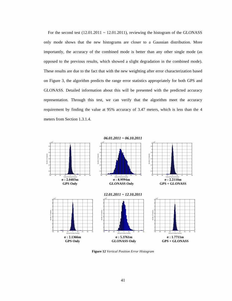
of each mode. With the enhanced range error modeling, Figure 12 shows the VPE histograms

of each mode and standard deviation for 10 days respectively. In order to represent the

improvement, we attached the results of incorrectly estimated range error on the top row and

the results of appropriately characterized range error on the bottom row. Even though the date

on which data were collected is different between the former and the latter experiments, the

difference did not affect the result significantly.

For the first test (06.01.2011 ~ 06.10.2011), in GPS only mode, the standard deviation is

close to the value in the GPS PAN Report in northern California, while GLONASS only mode

produces the large error and standard deviation. However, the standard deviation of GPS +

GLONASS mode is relatively greater than the one of GPS only mode. By examining

GLONASS only mode performance, we could infer that the incorrectly predicted GLONASS

error model affected the result of the position error in combined mode. The reason for this is

because when we applied the weight of GLONASS measurements to the weighted least square

solution, the error model, specifically the multipath model, had a lower value than it otherwise

would have.

41

For the second test (12.01.2011 ~ 12.01.2011), reviewing the histogram of the GLONASS

only mode shows that the new histograms are closer to a Gaussian distribution. More

importantly, the accuracy of the combined mode is better than any other single mode (as

opposed to the previous results, which showed a slight degradation in the combined mode).

These results are due to the fact that with the new weighting after error characterization based

on Figure 3, the algorithm predicts the range error statistics appropriately for both GPS and

GLONASS. Detailed information about this will be presented with the predicted accuracy

representation. Through this test, we can verify that the algorithm meet the accuracy

requirement by finding the value at 95% accuracy of 3.47 meters, which is less than the 4

meters from Section 1.3.1.4.

06.01.2011 ~ 06.10.2011

12.01.2011 ~ 12.10.2011

Figure 12 Vertical Position Error Histogram

-40 -30 -20 -10 0 10 20 30 400

0.5

1

1.5

2

2.5

3

3.5

4

4.5

5x 10

4

Vertical Position Error(m)

Num

ber o

f Sam

ples

-40 -30 -20 -10 0 10 20 30 400

0.5

1

1.5

2

2.5

3

3.5

4

4.5

5x 10

4

Vertical Position Error(m)

Num

ber o

f Sam

ples

-40 -30 -20 -10 0 10 20 30 400

0.5

1

1.5

2

2.5

3

3.5

4

4.5

5x 10

4

Vertical Position Error(m)

Num

ber o

f Sam

ples

-40 -30 -20 -10 0 10 20 30 400

1

2

3

4

5

6

7

8

9x 10

4

Vertical Position Error(m)

Num

ber o

f Sam

ples

-40 -30 -20 -10 0 10 20 30 400

1

2

3

4

5

6

7

8

9x 10

4

Vertical Position Error(m)

Num

ber o

f Sam

ples

-40 -30 -20 -10 0 10 20 30 400

1

2

3

4

5

6

7

8

9x 10

4

Vertical Position Error(m)

Num

ber o

f Sam

ples

σ : 8.9594m GLONASS Only

σ : 2.0403m GPS Only

σ : 2.2110m GPS + GLONASS

σ : 5.3761m GLONASS Only

σ : 2.1366m GPS Only

σ : 1.7711m GPS + GLONASS

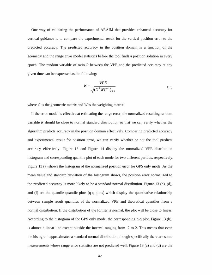
42

One way of validating the performance of ARAIM that provides enhanced accuracy for

vertical guidance is to compare the experimental result for the vertical position error to the

predicted accuracy. The predicted accuracy in the position domain is a function of the

geometry and the range error model statistics before the tool finds a position solution in every

epoch. The random variable of ratio R between the VPE and the predicted accuracy at any

given time can be expressed as the following:

3,3

1 )( −=

WGGVPER

T (13)

where G is the geometric matrix and W is the weighting matrix.

If the error model is effective at estimating the range error, the normalized resulting random

variable R should be close to normal standard distribution so that we can verify whether the

algorithm predicts accuracy in the position domain effectively. Comparing predicted accuracy

and experimental result for position error, we can verify whether or not the tool predicts

accuracy effectively. Figure 13 and Figure 14 display the normalized VPE distribution

histogram and corresponding quantile plot of each mode for two different periods, respectively.

Figure 13 (a) shows the histogram of the normalized position error for GPS only mode. As the

mean value and standard deviation of the histogram shows, the position error normalized to

the predicted accuracy is more likely to be a standard normal distribution. Figure 13 (b), (d),

and (f) are the quantile quantile plots (q-q plots) which display the quantitative relationship

between sample result quantiles of the normalized VPE and theoretical quantiles from a

normal distribution. If the distribution of the former is normal, the plot will be close to linear.

According to the histogram of the GPS only mode, the corresponding q-q plot, Figure 13 (b),

is almost a linear line except outside the interval ranging from -2 to 2. This means that even

the histogram approximates a standard normal distribution, though specifically there are some

measurements whose range error statistics are not predicted well. Figure 13 (c) and (d) are the

43

GLONASS only mode results. From these, we can infer easily that the algorithm did not

predict range error well. Even though there is the adverse effect of the GLONASS portion of

the solution, the combined mode provides a positive outcome as you see in Figure 13 (e) and

(f). Meanwhile, since the weighting matrix for the position solution is dependent on the range

error model which also affects the predicted accuracy, poor prediction against GLONASS

measurement is related to the inaccurate weighting matrix so that the accuracy of the

combined mode is greater than that of the GPS single mode. Therefore, it is necessary to

design an accurate multipath model for GLONASS.. Hence, we adjusted the smoothing time

coefficients as introduced in Section 2.1 and Figure 3. Figure 14 (a), (c), and (e) show the

histogram of normalized position error of each mode same as Figure 13 (a), (c), and (e).

Figure 14 (b), (d), and (f) present the quantile quantile plots which compares the result sample

distribution which is the normalized position error ratio and the theoretical normal standard

distribution same as Figure 13 (b), (d), and (f). Observing Figure 14 (b), (d), and (f) we can

notice that the middle part around the origin is almost fitted to linear line, and the mean and

standard deviation are more likely to be under standard normal distribution. As you see Figure

14 (c), the algorithm seems to predict the GLONASS range error statistics better than the

previous parameters setting (smoothing time coefficients). With the new GLONASS multipath

error model, the standard deviation of the normalized VPE distribution of GPS+GLONASS

mode is better than any other single mode.

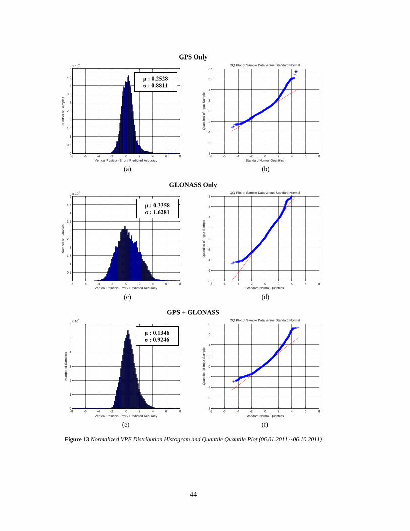
44

GPS Only

(a) (b)

GLONASS Only

(c) (d)

GPS + GLONASS

(e) (f)

Figure 13 Normalized VPE Distribution Histogram and Quantile Quantile Plot (06.01.2011 ~06.10.2011)

-8 -6 -4 -2 0 2 4 6 80

0.5

1

1.5

2

2.5

3

3.5

4

4.5

5x 10

4

Vertical Position Error / Predicted Accuracy

Num

ber o

f Sam

ples

-8 -6 -4 -2 0 2 4 6 8-8

-6

-4

-2

0

2

4

6

8

Standard Normal Quantiles

Qua

ntile

s of

Inpu

t Sam

ple

QQ Plot of Sample Data versus Standard Normal

-8 -6 -4 -2 0 2 4 6 80

0.5

1

1.5

2

2.5

3

3.5

4

4.5

5x 10

4

Vertical Position Error / Predicted Accuracy

Num

ber o

f Sam

ples

-8 -6 -4 -2 0 2 4 6 8-8

-6

-4

-2

0

2

4

6

8

Standard Normal Quantiles

Qua

ntile

s of

Inpu

t Sam

ple

QQ Plot of Sample Data versus Standard Normal

-8 -6 -4 -2 0 2 4 6 80

1

2

3

4

5

6x 10

4

Vertical Position Error / Predicted Accuracy

Num

ber o

f Sam

ples

-8 -6 -4 -2 0 2 4 6 8-8

-6

-4

-2

0

2

4

6

8

Standard Normal Quantiles

Qua

ntile

s of

Inpu

t Sam

ple

QQ Plot of Sample Data versus Standard Normal

μ : 0.2528 σ : 0.8811

μ : 0.3358 σ : 1.6281

μ : 0.1346 σ : 0.9246

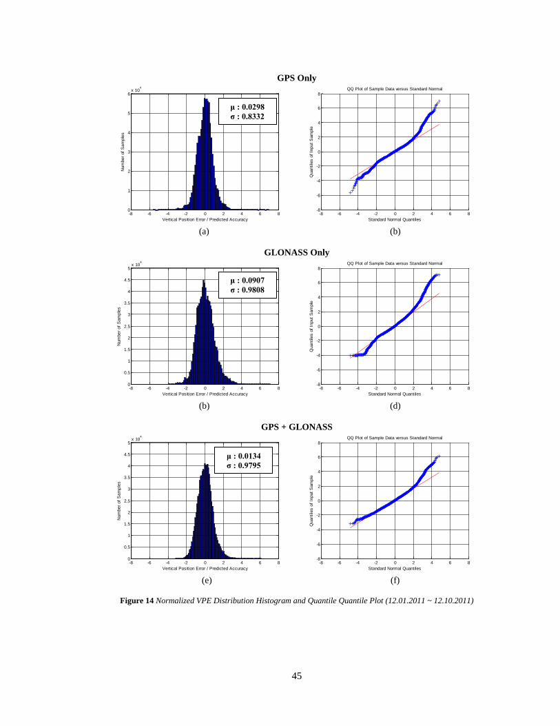
45

GPS Only

(a) (b)

GLONASS Only

(b) (d)

GPS + GLONASS

(e) (f)

Figure 14 Normalized VPE Distribution Histogram and Quantile Quantile Plot (12.01.2011 ~ 12.10.2011)

-8 -6 -4 -2 0 2 4 6 80

1

2

3

4

5

6x 10

4

Vertical Position Error / Predicted Accuracy

Num

ber o

f Sam

ples

-8 -6 -4 -2 0 2 4 6 8-8

-6

-4

-2

0

2

4

6

8

Standard Normal Quantiles

Qua

ntile

s of

Inpu

t Sam

ple

QQ Plot of Sample Data versus Standard Normal

-8 -6 -4 -2 0 2 4 6 80

0.5

1

1.5

2

2.5

3

3.5

4

4.5

5x 10

4

Vertical Position Error / Predicted Accuracy

Num

ber o

f Sam

ples

-8 -6 -4 -2 0 2 4 6 8-8

-6

-4

-2

0

2

4

6

8

Standard Normal Quantiles

Qua

ntile

s of

Inpu

t Sam

ple

QQ Plot of Sample Data versus Standard Normal

-8 -6 -4 -2 0 2 4 6 80

0.5

1

1.5

2

2.5

3

3.5

4

4.5

5x 10

4

Vertical Position Error / Predicted Accuracy

Num

ber o

f Sam

ples

-8 -6 -4 -2 0 2 4 6 8-8

-6

-4

-2

0

2

4

6

8

Standard Normal Quantiles

Qua

ntile

s of

Inpu

t Sam

ple

QQ Plot of Sample Data versus Standard Normal

μ : 0.0134 σ : 0.9795

μ : 0.0298 σ : 0.8332

μ : 0.0907 σ : 0.9808

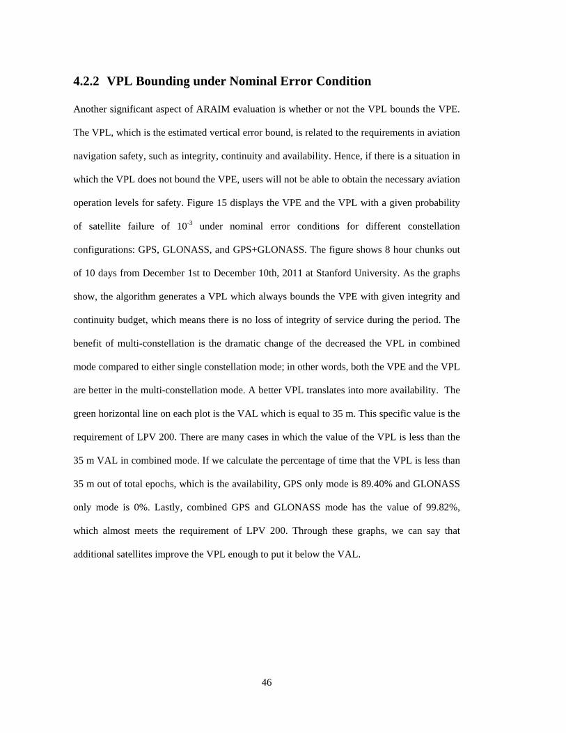
46

4.2.2 VPL Bounding under Nominal Error Condition

Another significant aspect of ARAIM evaluation is whether or not the VPL bounds the VPE.

The VPL, which is the estimated vertical error bound, is related to the requirements in aviation

navigation safety, such as integrity, continuity and availability. Hence, if there is a situation in

which the VPL does not bound the VPE, users will not be able to obtain the necessary aviation

operation levels for safety. Figure 15 displays the VPE and the VPL with a given probability

of satellite failure of 10-3 under nominal error conditions for different constellation

configurations: GPS, GLONASS, and GPS+GLONASS. The figure shows 8 hour chunks out

of 10 days from December 1st to December 10th, 2011 at Stanford University. As the graphs

show, the algorithm generates a VPL which always bounds the VPE with given integrity and

continuity budget, which means there is no loss of integrity of service during the period. The

benefit of multi-constellation is the dramatic change of the decreased the VPL in combined

mode compared to either single constellation mode; in other words, both the VPE and the VPL

are better in the multi-constellation mode. A better VPL translates into more availability. The

green horizontal line on each plot is the VAL which is equal to 35 m. This specific value is the

requirement of LPV 200. There are many cases in which the value of the VPL is less than the

35 m VAL in combined mode. If we calculate the percentage of time that the VPL is less than

35 m out of total epochs, which is the availability, GPS only mode is 89.40% and GLONASS

only mode is 0%. Lastly, combined GPS and GLONASS mode has the value of 99.82%,

which almost meets the requirement of LPV 200. Through these graphs, we can say that

additional satellites improve the VPL enough to put it below the VAL.

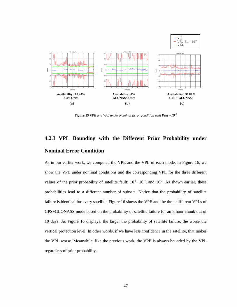
47

(a) (b) (c)

Figure 15 VPE and VPL under Nominal Error condition with Psat =10-3

4.2.3 VPL Bounding with the Different Prior Probability under

Nominal Error Condition

As in our earlier work, we computed the VPE and the VPL of each mode. In Figure 16, we

show the VPE under nominal conditions and the corresponding VPL for the three different

values of the prior probability of satellite fault: 10-5, 10-4, and 10-3. As shown earlier, these

probabilities lead to a different number of subsets. Notice that the probability of satellite

failure is identical for every satellite. Figure 16 shows the VPE and the three different VPLs of

GPS+GLONASS mode based on the probability of satellite failure for an 8 hour chunk out of

10 days. As Figure 16 displays, the larger the probability of satellite failure, the worse the

vertical protection level. In other words, if we have less confidence in the satellite, that makes

the VPL worse. Meanwhile, like the previous work, the VPE is always bounded by the VPL

regardless of prior probability.

0 1 2 3 4 5 6 7 8-150

-100

-50

0

50

100

150VPE and VPL

met

ers

Time(hrs)0 1 2 3 4 5 6 7 8

-150

-100

-50

0

50

100

150VPE and VPL

met

ers

Time(hrs)

0 1 2 3 4 5 6 7 8-150

-100

-50

0

50

100

150VPE and VPL

met

ers

Time(hrs)

Availability : 99.82% GPS + GLONASS

Availability : 0% GLONASS Only

Availability : 89.40% GPS Only

─ VPE ─ VPL Psat = 10-3 … VAL

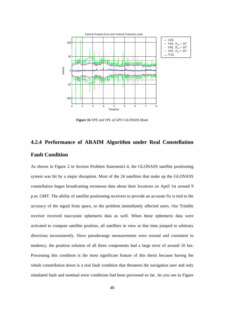
48

Figure 16 VPE and VPL of GPS+GLONASS Mode

4.2.4 Performance of ARAIM Algorithm under Real Constellation

Fault Condition

As shown in Figure 2 in Section Problem Statement1.4, the GLONASS satellite positioning

system was hit by a major disruption. Most of the 24 satellites that make up the GLONASS

constellation began broadcasting erroneous data about their locations on April 1st around 9

p.m. GMT. The ability of satellite positioning receivers to provide an accurate fix is tied to the

accuracy of the signal from space, so the problem immediately affected users. Our Trimble

receiver received inaccurate ephemeris data as well. When these ephemeris data were

activated to compute satellite position, all satellites in view at that time jumped to arbitrary

directions inconsistently. Since pseudorange measurements were normal and consistent in

tendency, the position solution of all three components had a large error of around 10 km.

Processing this condition is the most significant feature of this thesis because having the

whole constellation down is a real fault condition that threatens the navigation user and only

simulated fault and nominal error conditions had been processed so far. As you see in Figure

0 1 2 3 4 5 6 7 8

-100

-50

0

50

100

Vertical Position Error and Vertical Protection Level

met

ers

Time(hrs)

─ VPE ─ VPL Psat = 10-5 ─ VPL Psat = 10-4 ─ VPL Psat = 10-3

… VAL

49

17, which is the skyplot of GLONASS satellites in view around the 10 seconds when the

GLONASS event happened, you can verify a big jump in movement of satellites before and

after the event. The star dots are the satellite positions sampled by 1 second, specifically, the

blue star dots are the positions of each satellite prior to the event and the red star dots are the

positions of each satellite after the event. Note that the red box is the zoomed in view of

certain satellite position tracks used for clarifying the big jump in satellite position.

Figure 17 Sky Plot of GLONASS Satellites at Fault Event on April 1st, 2014

Figure 18 is the VPE and the VPL of GLONASS only mode for 2 days from April 1st to

April 2nd, which the ARAIM algorithm produced. The VPE suffers from large error due to

disrupted ephemeris data.

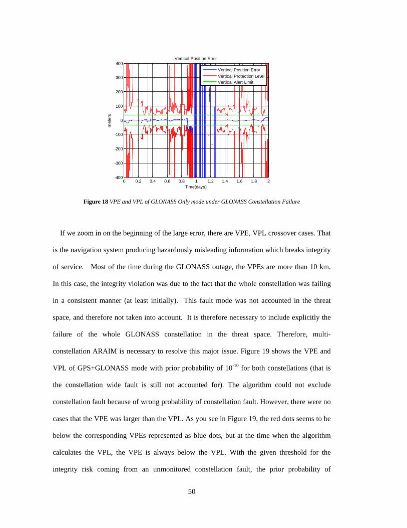
50

Figure 18 VPE and VPL of GLONASS Only mode under GLONASS Constellation Failure

If we zoom in on the beginning of the large error, there are VPE, VPL crossover cases. That

is the navigation system producing hazardously misleading information which breaks integrity

of service. Most of the time during the GLONASS outage, the VPEs are more than 10 km.

In this case, the integrity violation was due to the fact that the whole constellation was failing

in a consistent manner (at least initially). This fault mode was not accounted in the threat

space, and therefore not taken into account. It is therefore necessary to include explicitly the

failure of the whole GLONASS constellation in the threat space. Therefore, multi-

constellation ARAIM is necessary to resolve this major issue. Figure 19 shows the VPE and

VPL of GPS+GLONASS mode with prior probability of 10-10 for both constellations (that is

the constellation wide fault is still not accounted for). The algorithm could not exclude

constellation fault because of wrong probability of constellation fault. However, there were no

cases that the VPE was larger than the VPL. As you see in Figure 19, the red dots seems to be

below the corresponding VPEs represented as blue dots, but at the time when the algorithm

calculates the VPL, the VPE is always below the VPL. With the given threshold for the

integrity risk coming from an unmonitored constellation fault, the prior probability of

0 0.2 0.4 0.6 0.8 1 1.2 1.4 1.6 1.8 2-400

-300

-200

-100

0

100

200

300

400Vertical Position Error

met

ers

Time(days)

Vertical Position ErrorVertical Protection LevelVertical Alert Limit

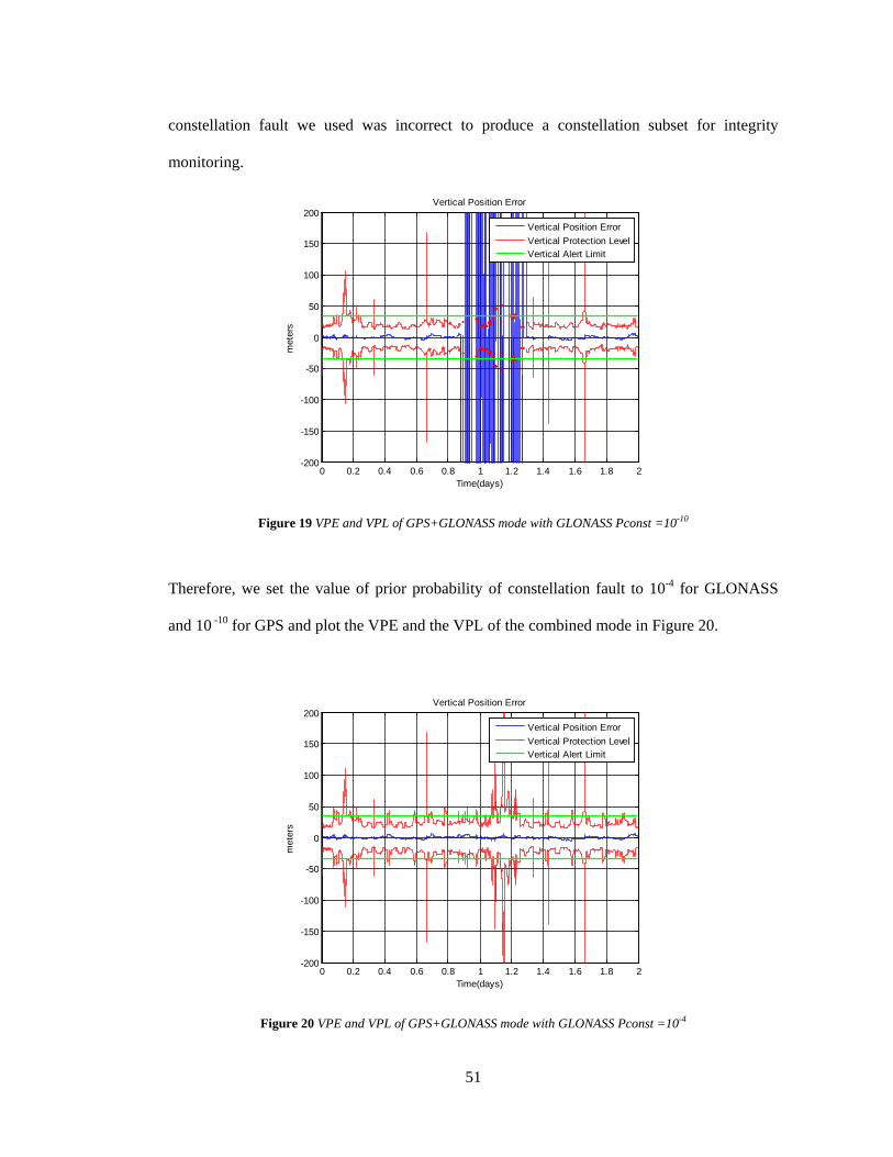
51

constellation fault we used was incorrect to produce a constellation subset for integrity

monitoring.

Figure 19 VPE and VPL of GPS+GLONASS mode with GLONASS Pconst =10-10

Therefore, we set the value of prior probability of constellation fault to 10-4 for GLONASS

and 10 -10 for GPS and plot the VPE and the VPL of the combined mode in Figure 20.

Figure 20 VPE and VPL of GPS+GLONASS mode with GLONASS Pconst =10-4

0 0.2 0.4 0.6 0.8 1 1.2 1.4 1.6 1.8 2-200

-150

-100

-50

0

50

100

150

200Vertical Position Error

met

ers

Time(days)

Vertical Position ErrorVertical Protection LevelVertical Alert Limit

0 0.2 0.4 0.6 0.8 1 1.2 1.4 1.6 1.8 2-200

-150

-100

-50

0

50

100

150

200Vertical Position Error

met

ers

Time(days)

Vertical Position ErrorVertical Protection LevelVertical Alert Limit

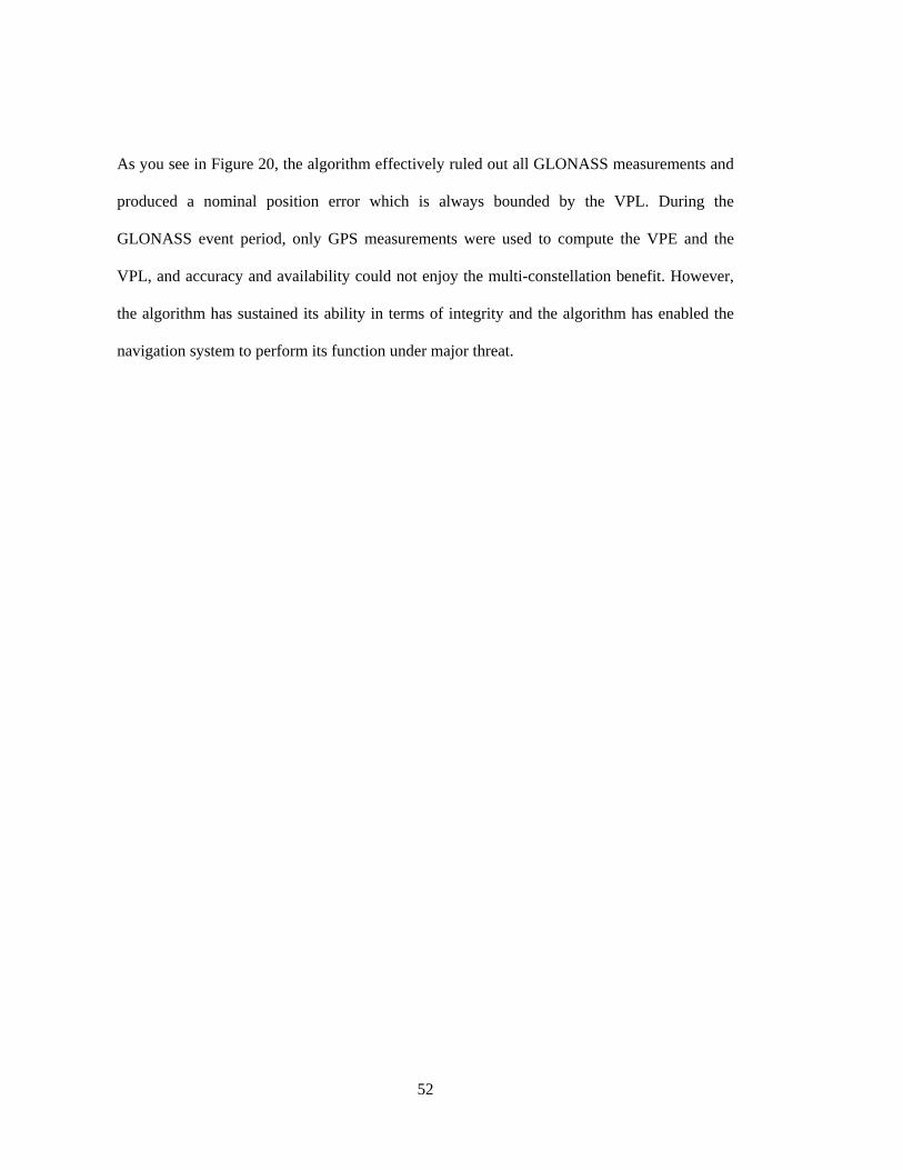
52

As you see in Figure 20, the algorithm effectively ruled out all GLONASS measurements and

produced a nominal position error which is always bounded by the VPL. During the

GLONASS event period, only GPS measurements were used to compute the VPE and the

VPL, and accuracy and availability could not enjoy the multi-constellation benefit. However,

the algorithm has sustained its ability in terms of integrity and the algorithm has enabled the

navigation system to perform its function under major threat.

53

Chapter 5 Conclusion

This thesis describes work performed to validate a multi-constellation ARAIM algorithm to

support vertical guidance for aircraft. Chapter 2 introduced ARAIM algorithm features such as,

range error modeling, procedure, considerations on integrating GPS and GLONASS signal

measurements, and the multiple fault assumption implementation. Chapter 3 presents the

evaluation method, setup, and data collection. Then the ARAIM prototype proposed in [19]

went through an extensive validation process. The present work computed the VPE and the

VPL for four months of data from 82 reference stations. It addressed two types of conditions

that would cover a range of possible situations in a real airborne system. The result of the

evaluation shows that the algorithm performed as we expected and protected users from

hazardously misleading information. In fault free conditions and the data fault condition, the

VPE was always less than the VPL, which did not break the integrity characteristics. However,

this test was limited because only measurements of a single constellation, GPS, were used and

the single satellite fault assumption was applied. Therefore, in Chapter 4 the enhanced multi-

constellation ARAIM algorithm was examined in different ways than the previous extensive

validation in Chapter 3. The present work conducted tests with extended constellations, i.e.,

GPS and GLONASS, through a GNSS receiver which can track multi-constellations under the

multiple faults assumption. Chapter 4 calculated the VPE and the VPL using the ARAIM

54

Evaluation tool for 10 days using both single constellation and multi-constellation

configurations. This evaluation verified two aspects of ARAIM capability: the predicting

accuracy ability and the VPL bounding. The algorithm computes position 100% of the time in

any combination of constellation mode and I also observed in all situations that the VPL

always over bounded the VPE as we expected. Even under the fault condition, the algorithm

performs well showing robust error bounding. Noticeably, the error model estimation

performance appeared to be constellation dependent, so it is necessary to design a reliable

error model for each constellation in order to provide better accuracy prediction. This is

confirmed by an attempt to refine the range error model one of the later tests. The new model

resulted in a better error characterization, and therefore in a more accurate position solution. In

addition, I implemented the multiple faults assumption by increasing the probability of

satellite failure. I showed how the prior probability of satellite fault influences the VPL. I have

seen that with large priors, adding satellites (in this case, a whole constellation) produces

smaller VPLs, therefore increasing availability. Moreover, due to the GLONASS event in

April 2014, I could test a real fault situation, which was a whole constellation failure. In this

evaluation, with an appropriate prior probability, the Multi-Constellation ARAIM tool

successfully filtered out the whole GLONASS measurement when the event occurred.

Eventually, more ranging sources from multi-constellations will guarantee narrower error

bounding than single constellation. Through these tests, we have shown that it is possible to

use Multi-Constellation ARAIM for vertical guidance in the near future.

Since, currently there are only two complete constellations (GPS, GLONASS), this thesis

processed the data of those two constellations. As new constellations are on the way to being

fully operational, the Multi-Constellation ARAIM evaluation tool should be updated

accordingly and tested with every complete constellation (GPS, GLONASS, Galileo, and

55

Beidou). Thus improved, this tool will further validate Multi-Constellation ARAIM as a

candidate for the provision of safety of life applications for aviation..

56

57

Bibliography

[1] P. Misra and P. Enge, Global Positioning System, Ganga-Jamuna Press, 2011.

[2] C. Hegarty and E. Chatre, “Evolution of the Global Navigation Stellite System (GNSS),”

in Proceedings of the IEEE, 2008.

[3] RTCA, Inc., SC-159, “Minimum Operational Performance Standards for Global

Positioning System/Wide Area Augmentation System Airborne Equipment,” RTCA/DO-

229C, Washington, 2001.

[4] RTCA, Inc., SC-159, “Minimum Aviation System Performance Standards for the Local

Area Augmentation System (LAAS),” RTCA/DO-245A, Washington, 2004.

[5] International Civil Aviation Organization (ICAO), in Annex 10 to the Convention on

International Civil Aviation International Standards and Recommended

Practices(SARPs), Volume I (Radio Navigation Aids), Montreal, Canada, 2007.

[6] Y. C. Lee, “Analysis of Range and Position Comparison Methods as a Means to Provide

GPS Integrity in the User Receiver,” Navigation Journal of the Institute of Navigation,

1986.

[7] B. W. Parkinson and P. Axelrad, “A Basis for the Development of Operational

Algorithms for Simplified GPS Integrity Checking,” in Proceedings of The Satellite

Division First Techinical Meeting, Institue of Navigation, Colorado Springs, 1987.

[8] M. A. Sturza and A. K. Brown, “Comparison of Fixed and Variable Threshold RAIM

Algorithms,” in Proceedings of the 4rd International Techinical Meeting of the Satellite

Division, Institue of Navigation, Colorado Springs, 1990.

58

[9] M. A. Sturza, “Navigation System Integrity Monitoring Using Redudant Measurements,”

Navigation, vol. 35, no. 4, pp. 483-501, 1988.

[10] R. G. Brown, “A Baseline GPS RAIM Scheme and a Note on the Equivalence of Three

RAIM Methods,” Navigation, vol. 39, no. 3, pp. 301-316, 1992.

[11] J. Angus, “RAIM with Multiple Faults,” Navigation, vol. 53, no. 4, pp. 249-257, 2006.

[12] T. Walter and P. Enge, “Weighted RAIM for Precision Approach,” in Proceedings of

ION-GPS, Palm Springs, 1995.

[13] J. Blanch, T. Walter and P. Enge, “RAIM with Optimal Integrity and Continuity

Allocations under Multiple Failures,” Aerospace and Electronic Systems, IEEE

Transactions on, vol. 46, no. 3, pp. 1235-1247, 2010.

[14] RTCA, Inc., SC-159, “Minimum Operational Performance Standards for Global

Positioning System/Wide Area Augmentation System Airborne Equipment,” RTCA/DO-

229D, 2006.

[15] Federal Aviation Administration, “GNSS Evolutionary Architecture Study, Phase I-panel

report,” 2008.

[16] Federal Aviation Administration, “GNSS Evolutionary Architecture Study, Phase II

Report”.

[17] Y. C. Lee, “Analysis of RAIM Using Multi Constellation to Provide LPV-200 Service

Worldwide,” in Proceddings of the ION GNSS, Portland, 2010.

[18] A. Ene, “Further Development of Galileo-GPS RAIM for Vertical Guidance,” in

Proceedings of the ION GNSS, Fort Worth, 2006.

[19] J. Blanch, M. Choi, T. Walter, P. Enge and K. Suzuki, “Prototyping Advanced RAIM for

Vertical Guidance,” in Proceedings of ION GNSS, Portland, 2010.

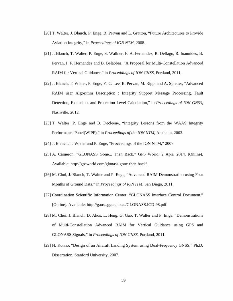
59

[20] T. Walter, J. Blanch, P. Enge, B. Pervan and L. Gratton, “Future Architectures to Provide

Aviation Integrity,” in Proceedings of ION NTM, 2008.

[21] J. Blanch, T. Walter, P. Enge, S. Wallner, F. A. Fernandez, R. Dellago, R. Ioannides, B.

Pervan, I. F. Hernandez and B. Belabbas, “A Proposal for Multi-Constellation Advanced

RAIM for Vertical Guidance,” in Proceddings of ION GNSS, Portland, 2011.

[22] J. Blanch, T. Wlater, P. Enge, Y. C. Lee, B. Pervan, M. Rippl and A. Spletter, “Advanced

RAIM user Algorithm Description : Integrity Support Message Processing, Fault

Detection, Exclusion, and Protection Level Calculation,” in Proceedings of ION GNSS,

Nashville, 2012.

[23] T. Walter, P. Enge and B. Decleene, “Integrity Lessons from the WAAS Integrity

Performance Panel(WIPP),” in Proceedings of the ION NTM, Anaheim, 2003.

[24] J. Blanch, T. Wlater and P. Enge, “Proceedings of the ION NTM,” 2007.

[25] A. Cameron, “GLONASS Gone... Then Back,” GPS World, 2 April 2014. [Online].

Available: http://gpsworld.com/glonass-gone-then-back/.

[26] M. Choi, J. Blanch, T. Walter and P. Enge, “Advanced RAIM Demonstration using Four

Months of Ground Data,” in Proceedings of ION ITM, San Diego, 2011.

[27] Coordination Scientific Information Center, “GLONASS Interface Control Document,”

[Online]. Available: http://gauss.gge.unb.ca/GLONASS.ICD-98.pdf.

[28] M. Choi, J. Blanch, D. Akos, L. Heng, G. Gao, T. Walter and P. Enge, “Demonstrations

of Multi-Constellation Advanced RAIM for Vertical Guidance using GPS and

GLONASS Signals,” in Proceedings of ION GNSS, Portland, 2011.

[29] H. Konno, “Design of an Aircraft Landing System using Dual-Frequency GNSS,” Ph.D.

Dissertation, Stanford University, 2007.

60