© 2008, 2012 Zachary S Tseng A-2 - 1

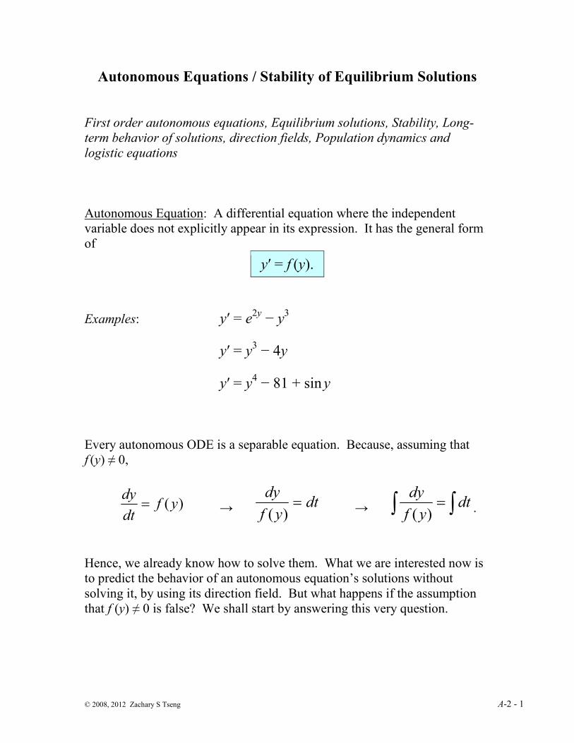
Autonomous Equations / Stability of Equilibrium Solutions

First order autonomous equations, Equilibrium solutions, Stability, Long-

term behavior of solutions, direction fields, Population dynamics and

logistic equations

Autonomous Equation: A differential equation where the independent

variable does not explicitly appear in its expression. It has the general form

of

y′ = f (y).

Examples: y′ = e2y

− y3

y′ = y3 − 4y

y′ = y4 − 81 + sin y

Every autonomous ODE is a separable equation. Because, assuming that

f (y) ≠ 0,

)(yfdt

dy= → dt

yf

dy=

)( → ∫∫ = dtyf

dy

)( .

Hence, we already know how to solve them. What we are interested now is

to predict the behavior of an autonomous equation’s solutions without

solving it, by using its direction field. But what happens if the assumption

that f (y) ≠ 0 is false? We shall start by answering this very question.

© 2008, 2012 Zachary S Tseng A-2 - 2

Equilibrium solutions

Equilibrium solutions (or critical points) occur whenever y′ = f (y) = 0. That

is, they are the roots of f (y). Any root c of f (y) yields a constant solution y =

c. (Exercise: Verify that, if c is a root of f (y), then y = c is a solution of

y′ = f (y).) Equilibrium solutions are constant functions that satisfy the

equation, i.e., they are the constant solutions of the differential equation.

Example: Logistic Equation of Population

21 yK

rryy

K

yry −=

−=′

Both r and K are positive constants. The solution y is the population

size of some ecosystem, r is the intrinsic growth rate, and K is the

environmental carrying capacity. The intrinsic growth rate is the

natural rate of growth of the population provided that the availability

of necessary resource (food, water, oxygen, etc) is limitless. The

environmental carrying capacity (or simply, carrying capacity) is the

maximum sustainable population size given the actual availability of

resource.

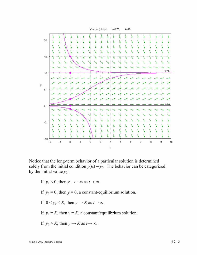
Without solving this equation, we will examine the behavior of its

solution. Its direction field is shown in the next figure.

© 2008, 2012 Zachary S Tseng A-2 - 3

Notice that the long-term behavior of a particular solution is determined

solely from the initial condition y(t0) = y0. The behavior can be categorized

by the initial value y0:

If y0 < 0, then y → − ∞ as t→ ∞.

If y0 = 0, then y = 0, a constant/equilibrium solution.

If 0 < y0 < K, then y → K as t→ ∞.

If y0 = K, then y = K, a constant/equilibrium solution.

If y0 > K, then y → K as t→ ∞.

© 2008, 2012 Zachary S Tseng A-2 - 4

Comment: In a previous section (applications: air-resistance) you learned an

easy way to find the limiting velocity without having to solve the differential

equation. Now we can see that the limiting velocity is just the equilibrium

solution of the motion equation (which is an autonomous equation). Hence

it could be found by setting v′ = 0 in the given differential equation and

solve for v.

Stability of an equilibrium solution

The stability of an equilibrium solution is classified according to the

behavior of the integral curves near it – they represent the graphs of

particular solutions satisfying initial conditions whose initial values, y0,

differ only slightly from the equilibrium value.

If the nearby integral curves all converge towards an equilibrium

solution as t increases, then the equilibrium solution is said to be

stable, or asymptotically stable. Such a solution has long-term

behavior that is insensitive to slight (or sometimes large) variations in

its initial condition.

If the nearby integral curves all diverge away from an equilibrium

solution as t increases, then the equilibrium solution is said to be

unstable. Such a solution is extremely sensitive to even the slightest

variations in its initial condition − as we can see in the previous

example that the smallest deviation in initial value results in totally

different behaviors (in both long- and short-terms).

Therefore, in the logistic equation example, the solution y = 0 is an unstable

equilibrium solution, while y = K is an (asymptotically) stable equilibrium

solution.

© 2008, 2012 Zachary S Tseng A-2 - 5

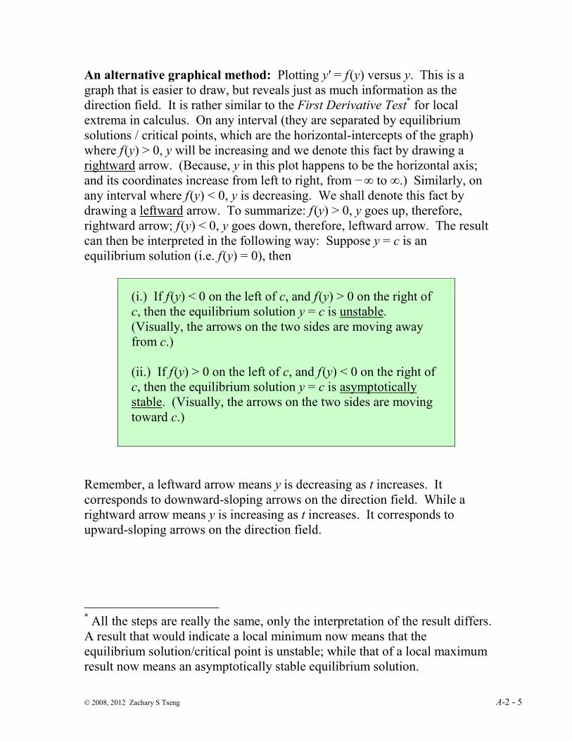
An alternative graphical method: Plotting y′ = f (y) versus y. This is a

graph that is easier to draw, but reveals just as much information as the

direction field. It is rather similar to the First Derivative Test* for local

extrema in calculus. On any interval (they are separated by equilibrium

solutions / critical points, which are the horizontal-intercepts of the graph)

where f (y) > 0, y will be increasing and we denote this fact by drawing a

rightward arrow. (Because, y in this plot happens to be the horizontal axis;

and its coordinates increase from left to right, from − ∞ to ∞.) Similarly, on

any interval where f (y) < 0, y is decreasing. We shall denote this fact by

drawing a leftward arrow. To summarize: f (y) > 0, y goes up, therefore,

rightward arrow; f (y) < 0, y goes down, therefore, leftward arrow. The result

can then be interpreted in the following way: Suppose y = c is an

equilibrium solution (i.e. f (y) = 0), then

(i.) If f (y) < 0 on the left of c, and f (y) > 0 on the right of

c, then the equilibrium solution y = c is unstable.

(Visually, the arrows on the two sides are moving away

from c.)

(ii.) If f (y) > 0 on the left of c, and f (y) < 0 on the right of

c, then the equilibrium solution y = c is asymptotically

stable. (Visually, the arrows on the two sides are moving

toward c.)

Remember, a leftward arrow means y is decreasing as t increases. It

corresponds to downward-sloping arrows on the direction field. While a

rightward arrow means y is increasing as t increases. It corresponds to

upward-sloping arrows on the direction field.

* All the steps are really the same, only the interpretation of the result differs.

A result that would indicate a local minimum now means that the

equilibrium solution/critical point is unstable; while that of a local maximum

result now means an asymptotically stable equilibrium solution.

© 2008, 2012 Zachary S Tseng A-2 - 6

As an example, let us apply this alternate method on the same logistic

equation seen previously: y′ = ry − (r / K) y2, r = 0.75, K = 10.

The y′-versus-y plot is shown below.

As can be seen, the equilibrium solutions y = 0 and y = K = 10 are the

two horizontal-intercepts (confusingly, they are the y-intercepts, since

the y-axis is the horizontal axis). The arrows are moving apart from

y = 0. It is, therefore, an unstable equilibrium solution. On the other

hand, the arrows from both sides converge toward y = K. Therefore, it

is an (asymptotically) stable equilibrium solution.

© 2008, 2012 Zachary S Tseng A-2 - 7

Example: Logistic Equation with (Extinction) Threshold

yK

y

T

yry

−

−−=′ 11

Where r, T, and K are positive constants: 0 < T < K.

The values r and K still have the same interpretations, T is the extinction

threshold level below which the species is endangered and eventually

become extinct. As seen above, the equation has (asymptotically) stable

equilibrium solutions y = 0 and y = K. There is an unstable equilibrium

solution y = T.

© 2008, 2012 Zachary S Tseng A-2 - 8

The same result can, of course, be obtained by looking at the y′-versus-y plot

(in this example, T = 5 and K = 10):

We see that y = 0 and y = K are (asymptotically) stable, and y = T is unstable.

Once again, the long-term behavior can be determined just by the initial

value y0:

If y0 < 0, then y → 0 as t→ ∞.

If y0 = 0, then y = 0, a constant/equilibrium solution.

If 0 < y0 < T, then y → 0 as t→ ∞.

If y0 = T, then y = T, a constant/equilibrium solution.

If T < y0 < K, then y → K as t→ ∞.

If y0 = K, then y = K, a constant/equilibrium solution.

If y0 > K, then y → K as t→ ∞.

Semistable equilibrium solution

A third type of equilibrium solutions exist. It exhibits a half-and-half

behavior. It is demonstrated in the next example.

© 2008, 2012 Zachary S Tseng A-2 - 9

Example: y′ = y3 − 2 y

2

The equilibrium solutions are y = 0 and 2. As can be seen below,

y = 2 is an unstable equilibrium solution. The interesting thing here,

however, is the equilibrium solution y = 0 (which corresponding a

double-root of f (y).

Notice the behavior of the integral curves near the equilibrium solution y = 0.

The integral curves just above it are converging to it, like it is an

asymptotically stable equilibrium solution, but all the integral curves below

it are moving away and diverging to −∞, a behavior associated with an

unstable equilibrium solution. A behavior such like this defines a semistable

equilibrium solution.

© 2008, 2012 Zachary S Tseng A-2 - 10

An equilibrium solution is semistable if y′ has the same sign on both

adjacent intervals. (In our analogy with the First Derivative Test, if the

result would indicate that a critical point is neither a local maximum nor a

minimum, then it now means we have a semistable equilibrium solution.

(iii.) If f (y) > 0 on both sides of c, or f (y) < 0 on both

sides of c, then the equilibrium solution y = c is

semistable. (Visually, the arrows on one side are moving

toward c, while on the other side they are moving away

from c.)

Comment: As we can see, it is actually not necessary to graph anything in

order to determine stability. The only thing we need to make the

determination is the sign of y′ on the interval immediately to either side of an

equilibrium solution (a.k.a. critical point), then just apply the above-

mentioned rules. The steps are otherwise identical to the first derivative test:

breaking the number line into intervals using critical points, evaluate y′ at an

arbitrary point within each interval, finally make determination based on the

signs of y′. This is our version of the first derivative test for classifying

stability of equilibrium solutions of an autonomous equation. (The graphing

methods require more work but also will provide more information –

unnecessary for our purpose here – such as the instantaneous rate of change

of a particular solution at any point.)

Computationally, stability classification tells us the sensitivity (or lack

thereof) to slight variations in initial condition of an equilibrium solution.

An unstable equilibrium solution is very sensitive to deviations in the initial

condition. Even the slightest change in the initial value will result in a very

different asymptotical behavior of the particular solution. An asymptotically

stable equilibrium solution, on the other hand, is quite tolerant of small

changes in the initial value − a slight variation of the initial value will still

result in a particular solution with the same kind of long-term behavior. A

semistable equilibrium solution is quite insensitive to slight variation in the

initial value in one direction (toward the converging, or the stable, side).

But it is extremely sensitive to a change of the initial value in the other

direction (toward the diverging, or the unstable, side).

© 2008, 2012 Zachary S Tseng A-2 - 11

Exercises A-2.1:

1 − 8 Find and classify all equilibrium solutions of each equation below.

1. y′ = 100 y − y3

2. y′ = y3 − 4y

3. y′ = y(y − 1)( y − 2)(y − 3)

4. y′ = sin y

5. y′ = cos2(π y / 2)

6. y′ = 1 − e y

7. y′ = (3y2 −2y − 1)e

−2y

8. y′ = y(y − 1)2(3 − y)(y − 5)

2

9. For each of problems 1 through 8, determine the value to which y will

approach as t increases if (a) y0 = −1, and (b) y0 = π.

10. Consider the air-resistance equation from an earlier example,

100v′ = 10000 − 4v2. (i) Find and classify its equilibrium solutions. (ii)

Given y(t0) = 0, determine the range of y(t). (iii) Given y(8) = −60,

determine the range of y(t).

11. Verify the fact that every first order linear ODE with constant

coefficients only is also an autonomous equation (and, therefore, is also a

separable equation).

12. Give an example of an autonomous equation having no (real-valued)

equilibrium solution.

13. Give an example of an autonomous equation having exactly n

equilibrium solutions (n ≥ 1).

© 2008, 2012 Zachary S Tseng A-2 - 12

Answers A-2.1:

1. y = 0 (unstable), y = ±10 (asymptotically stable)

2. y = 0 (asymptotically stable), y = ±2 (unstable)

3. y = 0 and y = 2 (asymptotically stable), y = 1 and y = 3 (unstable)

4. y = 0, ±2π, ±4π, … (unstable), y = ±π, ±3π, ±5π, … (asymptotically stable)

5. y = ±1, ±3, ±5, … (all are semistable)

6. y = 0 (asymptotically stable)

7. y = −1/3 (asymptotically stable), y = 1 (unstable)

8. y = 0 (unstable), y = 1 and y = 5 (semistable), y = 3 (asymptotically stable)

9. (1) −10, 10; (2) 0, ∞; (3) 0, ∞; (4) − π, π; (5) −1, 5; (6) 0, 0;

(7) −1/3, ∞; (8) −∞, 3.

10. (i) y = −50 (unstable) and y = 50 (asymptotically stable); (ii) (−50, 50);

(iii) (−∞,−50)

11. For any constants α and β, y′ + αy = β can be rewritten as y′ = β − αy,

which is autonomous (and separable).

12. One example (there are infinitely many) is y′ = e y.

13. One of many examples is y′ = (y − 1)( y − 2)(y − 3)…(y − n).

© 2008, 2012 Zachary S Tseng A-2 - 13

Exact Equations

An exact equation is a first order differential equation that can be written in

the form

M(x,y) + N(x,y) y′ = 0,

provided that there exists a function ψ(x,y) such that

),( yxMx=

∂∂ψ

and ),( yxNy=

∂∂ψ

.

Note 1: Often the equation is written in the alternate form of

M(x,y) dx + N(x,y) dy = 0.

Theorem (Verification of exactness): An equation of the form

M(x,y) + N(x,y) y′ = 0

is an exact equation if and only if

x

N

y

M

∂∂

=∂∂

.

Note 2: If M(x) is a function of x only, and N(y) is a function of y only, then

trivially x

N

y

M

∂∂

==∂∂

0 . Therefore, every separable equation,

M(x) + N(y) y′ = 0,

can always be written, in its standard form, as an exact equation.

© 2008, 2012 Zachary S Tseng A-2 - 14

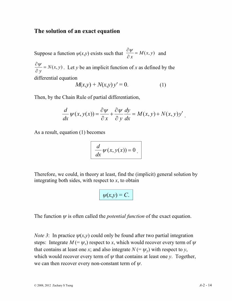
The solution of an exact equation

Suppose a function ψ(x,y) exists such that ),( yxMx=

∂∂ψ

and

),( yxNy=

∂∂ψ

. Let y be an implicit function of x as defined by the

differential equation

M(x,y) + N(x,y) y′ = 0. (1)

Then, by the Chain Rule of partial differentiation,

yyxNyxMdx

dy

yxxyx

dx

d′+=

∂∂

+∂∂

= ),(),())(,(ψψ

ψ .

As a result, equation (1) becomes

0))(,( =xyxdx

dψ .

Therefore, we could, in theory at least, find the (implicit) general solution by

integrating both sides, with respect to x, to obtain

ψ(x,y) = C.

The function ψ is often called the potential function of the exact equation.

Note 3: In practice ψ(x,y) could only be found after two partial integration

steps: Integrate M (= ψx) respect to x, which would recover every term of ψ

that contains at least one x; and also integrate N (= ψy) with respect to y,

which would recover every term of ψ that contains at least one y. Together,

we can then recover every non-constant term of ψ.

© 2008, 2012 Zachary S Tseng A-2 - 15

Note 4: In the context of multi-variable calculus, the solution of an exact

equation gives a certain level curve of the function z = ψ(x,y).

Comment: Students familiar with vector calculus would no doubt realize

that the calculation needed to verify and solve an exact equation is

essentially identical to the process used to verify a 2-dimensional

conservative vector field and to find the underlying potential function of the

vector field from its gradient vector.

© 2008, 2012 Zachary S Tseng A-2 - 16

Example: Solve the equation

(y4 − 2) + 4xy

3 y′ = 0

First identify that M(x,y) = y4 − 2, and N(x,y) = 4xy

3.

Then make sure that it is indeed an exact equation:

34y

y

M=

∂∂

and 34y

x

N=

∂∂

Finally find ψ(x,y) using partial integrations. First, we integrate M

with respect to x. Then integrate N with respect to y.

∫ ∫ +−=−== )(2)2(),(),( 1

44 yCxxydxydxyxMyxψ ,

∫ ∫ +=== )(4),(),( 2

43 xCxydyxydyyxNyxψ .

Combining the result, we see that ψ(x,y) must have 2 non-constant

terms: xy4 and −2x. That is, the (implicit) general solution is:

xy4 − 2x = C.

Now suppose there is the initial condition y(−1) = 2. To find the

(implicit) particular solution, all we need to do is to substitute x = −1

and y = 2 into the general solution. We then get C = −14.

Therefore, the particular solution is xy4 − 2x = −14.

© 2008, 2012 Zachary S Tseng A-2 - 17

Example: Solve the initial value problem

0)ln)cos(()2)cos(( =+++++ dyexxyxdxxx

yxyy y

, y(1) = 0.

First, we see that xx

yxyyyxM 2)cos(),( ++= and

yexxyxyxN ++= ln)cos(),( .

Verifying:

xxyxyxy

y

M 1)cos()sin( ++−=

∂∂

=x

xyxyxyx

N 1)cos()sin( ++−=

∂∂

Integrate to find the general solution:

)(ln)sin(2)cos(),( 1

2 yCxxyxydxxx

yxyyyx +++=

++= ∫ψ ,

as well,

( ) )(ln)sin(ln)cos(),( 2 xCexyxydyexxyxyx yy +++=++= ∫ψ .

Hence, sin xy + y ln x + e y + x

2 = C.

Apply the initial condition: x = 1 and y = 0:

C = sin 0 + 0 ln (1) + e 0 + 1 = 2

The particular solution is then sin xy + y ln x + e y + x

2 = 2.

© 2008, 2012 Zachary S Tseng A-2 - 18

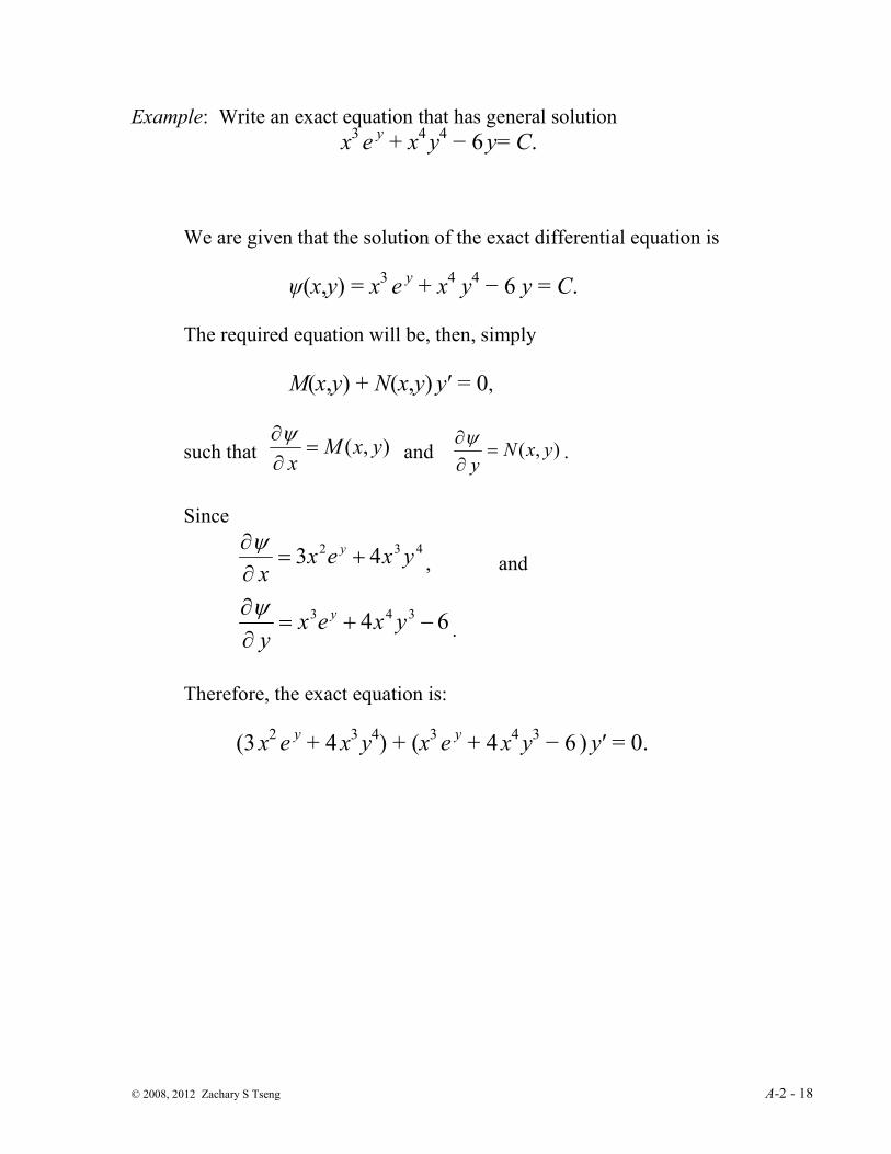
Example: Write an exact equation that has general solution

x3 e

y + x

4 y

4 − 6 y= C.

We are given that the solution of the exact differential equation is

ψ(x,y) = x3 e

y + x

4 y

4 − 6 y = C.

The required equation will be, then, simply

M(x,y) + N(x,y) y′ = 0,

such that ),( yxMx=

∂∂ψ

and ),( yxNy=

∂∂ψ

.

Since

432 43 yxexx

y +=∂∂ψ

, and

64 343 −+=∂∂

yxexy

yψ.

Therefore, the exact equation is:

(3 x2 e

y + 4 x

3 y

4) + (x

3 e y + 4 x

4 y

3 − 6 ) y′ = 0.

© 2008, 2012 Zachary S Tseng A-2 - 19

Summary: Exact Equations

M(x,y) + N(x,y) y′ = 0

Where there exists a function ψ(x,y) such that

),( yxMx=

∂∂ψ

and ),( yxNy=

∂∂ψ

.

1. Verification of exactness: it is an exact equation if and only if

x

N

y

M

∂∂

=∂∂

.

2. The general solution is simply

ψ(x,y) = C.

Where the function ψ(x,y) can be found by combining the result of the

two integrals (write down each distinct term only once, even if it

appears in both integrals):

∫= dxyxMyx ),(),(ψ , and

∫= dyyxNyx ),(),(ψ .

© 2008, 2012 Zachary S Tseng A-2 - 20

Exercises A-2.2:

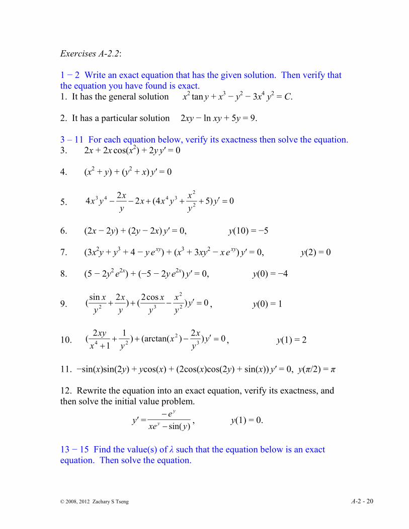
1 − 2 Write an exact equation that has the given solution. Then verify that

the equation you have found is exact.

1. It has the general solution x2 tan y + x

3 − y

2 − 3x

4 y

2 = C.

2. It has a particular solution 2xy − ln xy + 5y = 9.

3 – 11 For each equation below, verify its exactness then solve the equation.

3. 2x + 2x cos(x2) + 2y y′ = 0

4. (x2 + y) + (y

2 + x) y′ = 0

5. 0)54(22

42

23443 =′+++−− y

y

xyxx

y

xyx

6. (2x − 2y) + (2y − 2x) y′ = 0, y(10) = −5

7. (3x2y + y

3 + 4 − y e

xy) + (x

3 + 3xy

2 − x e

xy) y′ = 0, y(2) = 0

8. (5 − 2y2

e2x

) + (−5 − 2y e2x

) y′ = 0, y(0) = −4

9. 0)cos2

()2sin

(2

2

32=′−++ y

y

x

y

x

y

x

y

x, y(0) = 1

10. 0)2

)(arctan()1

1

2(

3

2

24=′−++

+y

y

xx

yx

xy, y(1) = 2

11. −sin(x)sin(2y) + ycos(x) + (2cos(x)cos(2y) + sin(x)) y′ = 0, y(π/2) = π

12. Rewrite the equation into an exact equation, verify its exactness, and

then solve the initial value problem.

y′ =)sin(yxe

ey

y

−−

, y(1) = 0.

13 − 15 Find the value(s) of λ such that the equation below is an exact

equation. Then solve the equation.

© 2008, 2012 Zachary S Tseng A-2 - 21

13. 0)3()1

2( 26

2

35 =′−+− yyxx

yx λλ

14. (λ y sec2(2xy) − λ xy

2) + (2x sec

2(2xy) − λ x

2y) y′ = 0

15. (10y4 − 6xy + 6x

2sin(x

3)) + (40xy

3 − 3x

2 + λ cos(x

3)) y′ = 0

16. Show that a first order linear equation y′ + p(t) y = g(t) is usually not

also an exact equation. But it becomes an exact equation after multiplied

through by its integrating factor. That is, the modified equation

µ(t) y′ + µ(t)p(t) y = µ(t)g(t), where ∫=

dttp

et)(

)(µ , will be an exact equation.

© 2008, 2012 Zachary S Tseng A-2 - 22

Answers A-2.2:

1. (2x tan y + 3x2 − 12x

3y

2) + (x

2 sec

2 y − 2y − 6x

4y ) y′ = 0

2. 0)51

2()1

2( =′+−+− yy

xx

y

3. x2 + y

2 + sin(x

2) = C

4. Cy

xyx

=++33

33

5. Cyxy

xyx =+−− 52

244

6. x2 – 2xy + y

2 = 225

7. x3y + xy

3 + 4x − e

xy = 7

8. 5x − 5y − y2

e2x

= 4

9. 1cos 2

2−=+

−y

x

y

x

10. 4

12)arctan(

2

2 +=+

πy

xxy

11. cos(x)sin(2y) + ysin(x) = π

12. The equation is e y + (x e

y − sin y) y′ = 0; x e

y + cos y = 2

13. λ = 3; x6y

3 + x

−1 − 3y = C

14. λ = 2; tan(2xy) − x2 y

2 = C

15. λ = 0; 10xy4 − 3x

2y − 2cos(x

3) = C