INTERNATIONAL JOURNAL of SMART GRID S. Bhongade and V. P. Parmar, Vol.2, No.2, 2018

Automatic Generation Control of Two-Area ST-

Thermal Power System using Jaya Algorithm

S. Bhongade*‡, Vishnu P Parmar**

*Department of Electrical Engineering, Faculty of Department of Electrical Engineering, S G S Institute of Technology &

Science, Indore,23, park road, Indore-452003 M.P-INDIA

** Department of Electrical Engineering, Faculty of Department of Electrical Engineering, S G S Institute of Technology &

Science, Indore,23, park road, Indore-452003 M.P-INDIA

‡ Corresponding Author; S G S Institute of Technology & Science, Indore,23, park road, Indore-452003 M.P-INDIA

, Tel: +91 7312582201,

Fax: +91 7312432540,bhongadesandeep@gmail.com

Received: 14.03.2018 Accepted:30.03.2018

Abstract- This article present automatic generation control (AGC) of a two area thermal system incorporating solar thermal

power plant (STPP) in one of the areas. The performance of the conventional two area system is compared with the proposed

system. Similarly, the performances of integral (I), proportional plus integral (PI), and proportional plus integral plus

derivative (PID) controller are evaluated in the system with STPP. For optimization of the proposed system, a new

optimization technique, i.e. Jaya Algorithm is used for the optimization of secondary controller gains. Examinations uncover

that Jaya optimized PID controller’s performance is better as compared to integral and proportional integral control. Better

dynamic performances like settling time, overshoot, undershoot is achieved by Jaya algorithm for the proposed system.

Further, robustness of the systems are studied by changing all the system parameter from -25% to 25%. Analysis reveals that

Jaya algorithm based PID controller gains are quite robust and need not be reset for large variations in system parameters.

Keywords Automatic Generation Control, Solar Thermal Power plant, Area control error, Integral Square Error, Settling time,

Over shoot, Under shoot, Jaya algorithm.

1. Introduction

The objective of the AGC is to make system frequency

stable and tie line power deviation zero for reliable and

efficient operation of the power plant. Automatic generation

control plays a vital role in power systems in maintaining

scheduled tie line power flow and specified frequency during

the normal operating condition as well as under small

perturbation [1-4].The main function of AGC is proper

selection of secondary controller gain. Frequency control is

the biggest issue because if frequency fluctuates in power

plant, speed keeps on changing and performance of power

plant will be disturbed. A Lot of work has been done earlier

on AGC but their focus was on conventional generation

(Thermal generation) [5-8] .These literature surveys are not

based on renewable energy source and no attention has been

paid to non conventional energy sources. Due to rapidly

decreasing conventional energy resources and carbon

emission issues, there is a need to find some other sources so

that future energy demand can be met. Solar and wind energy

sources are such options and solar energy has large potential.

From recent studies, it is said that it has potential to be a

source of the future. There are many problems with

availability of non renewable energy resources, which made

renewable energy sources the present research issue. Das et

al. [9] Describes the concept of integration of the solar

thermal power plant for AGC, but their work is limited to an

isolated system only. Solar energy is the huge source of the

clean energy and transformation of solar energy into electric

energy does not give off greenhouse gases, also these

renewable energies cut down the consumption of

conventional sources of energy. Hence, automatic generation

control of a multi-area system with STPP is important for

further studies.

There are two control modes in AGC, primary and

secondary control. Primary control is very fast and the

secondary control is slow as compared to primary control.

Nowadays, almost all studies on AGC are based on the

INTERNATIONAL JOURNAL of SMART GRID S. Bhongade and V. P. Parmar, Vol.2, No.2, 2018

100

design of the secondary controller. Many optimization

methods have been studied for controller gain such as a

Bacterial foraging optimization algorithm (BFOA) [10],

Particle Swarm Optimization (PSO) [11], Genetic Algorithm

(GA) [12], Firefly Algorithm (FA) [13], Artificial Neural

Network (ANN) [14], Differential evolution (DE) [15], fuzzy

logic [16], grey wolf optimization (GWO), flower pollination

algorithm (FPA) and many more. All the evolutionary and

swarm intelligence optimization techniques need appropriate

tuning of algorithm, specific parameters in addition to tuning

of common controlling parameters. The proper tuning of

these parameters is very much necessary.

Improper tuning of these parameters may increase the

computational cost or tendency towards the local optimal

solution. Hence, to avoid tuning problems of different

algorithm specific parameters, teaching learning based

optimization algorithm [17] was proposed. Keeping in view

good performance of the TLBO another very simple and new

algorithm which is specific parameter less and flexible

optimization method, i.e. JAYA ALGORITHM was

proposed by R.V. Rao [18] which is quite more simpler so it

is named as ‘JAYA’(means triumph originated from

Sanskrit),as it doesn’t consider any specific algorithm

parameter. Jaya algorithm considers the best and worst

solution among the whole population for update [19]. So it

becomes very easy and it has better convergence towards

global optimum point.

Following is the main objective of this work:

(a) Modeling and integration of solar thermal power

plant with two area thermal systems for AGC.

(b) Application of the Jaya algorithm for the

optimization of controller gains in two area system.

(c) Comparison of dynamic responses of frequency and

tie line power deviation with and without STPP to find the

best solution.

(d) Comparison of integral and PI controller with PID

controller.

(e) Sensitivity analysis of the system in the presence of

solar thermal power plant.

2. System Modelling

Two area thermal power systems are considered for

AGC. Value of specified parameter has been taken from

[20]. In Fig. 2 Solar Thermal Power Plant is used.

2.1. Thermal Power System

Thermal Power System consists of two areas Area1 and

Area2. Different values of parameters have been taken such

as time constants and other to make the analysis realistic.

Table 1 shows the transfer function of different components

present in the system.

Area Control Error (ACE) is the linear combination of

frequency deviation and change in tie line power. ACE is

taken as input to the PID controllers.

111 wBPACE tie (1)

222 wBPACE tie (2)

Where, 1

1

1

1D

RB and

2

2

2

1D

RB

The output of the PID controllers are obtained as given

below

1111111 ACEdt

dKACEKACEKu DIP (3)

2222222 ACEdt

dKACEKACEKu DIP (4)

Solar collector

oTI

LU

iTv

oA

eT

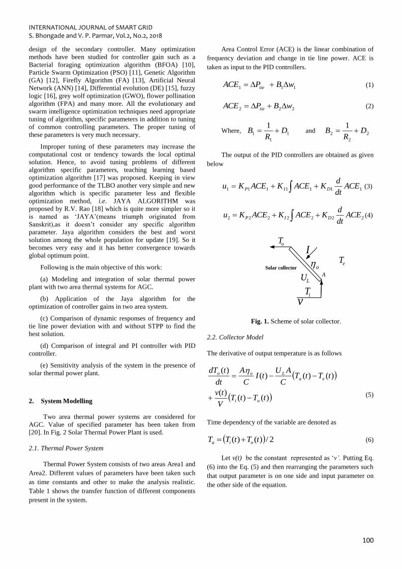
Fig. 1. Scheme of solar collector.

2.2. Collector Model

The derivative of output temperature is as follows

)()()(

)()()()(

tTtTV

tv

tTtTC

AUtI

C

A

dt

tdT

oi

eaLoo

(5)

Time dependency of the variable are denoted as

2/)()( tTtTT oia (6)

Let v(t) be the constant represented as ‘v’. Putting Eq.

(6) into the Eq. (5) and then rearranging the parameters such

that output parameter is on one side and input parameter on

the other side of the equation.

INTERNATIONAL JOURNAL of SMART GRID S. Bhongade and V. P. Parmar, Vol.2, No.2, 2018

101

)(

)(2

)()(2)(

)(

tTC

AU

tTC

AU

V

vtI

C

AtT

V

v

C

AU

td

tdT

eL

iLo

oLo

(7)

Taking Laplace of the above equation and the outcome

of the Laplace transform is as given below.

)()(2

)()(2

)0()(

sTC

AUsT

C

AU

V

v

sIC

AsT

V

v

C

AUTssT

eL

iL

o

oL

oo

(8)

Rearranging above equation …

)(1

)(21

)(1

)0(1

)(

sTC

AU

sT

TsT

C

AU

V

v

sT

T

sIC

A

sT

TT

T

TsT

eL

s

s

iL

s

s

o

s

s

o

s

s

o

(9)

where, Ts is the time constant of the collector and given by

V

v

C

AUT

L

s

2

1

To calculate the transfer function for a given input,

other inputs are considered and initial conditions are assumed

to be zero. The transfer function for each input is

C

A

sT

T

sI

sTsW o

s

so

1)(

)()(1

(10)

C

AU

V

v

sT

T

sT

sTsW L

s

s

i

o

21)(

)()(2

(11)

C

AU

sT

T

sT

sTsW L

s

s

e

o

)1()(

)()(3

(12)

Similarly, initial condition response can be obtained by

s

s

o

o

osT

T

T

sTsW

1)0(

)()(

(13)

Hence the following equation gives the outlet

temperature of the collector considering the effects of the

inputs and the initial temperature.

)()()()(

)()()()()(

32

1

sTsWsTsW

sIsWsTsWsT

ei

ooo

(14)

This is the collector model when the heat transfer rate is

taken constant.

Various atmospheric parameters add their effects on

solar collector models such as solar irradiance, inlet

temperature and environment temperature, etc. But the major

effect is of solar irradiance. So for simplified model only

solar irradiance is considered. Hence transfer function of

solar field with respect to solar irradiance is given by Eq.

(15).

sT

KsG

s

s

1)( (15)

Where, Ks is the gain value and Ts is the time constant

of the solar field. Hence, steam is produced in heat

exchanger which drives the turbine. Solar irradiation is

taken as 0.4 and transportation delay is taken for the

various processes of STPP.

Table1 Component transfer function of two area system

Components Transfer Function

Governor

gg sT

TF

1

1

Turbine

tt sT

TF

1

1

Load and machine

DHs 1

INTERNATIONAL JOURNAL of SMART GRID S. Bhongade and V. P. Parmar, Vol.2, No.2, 2018

102

2.3. Solar Thermal Power Plant

Renewable energy sources are current issue of research

[21, 22]. In view of system efficiency and keeping in mind

the protection of the surrounding environment, renewable

energy has gained the importance day by day. It is very

important to reap solar energy effectively by developing

solar collectors. In this article STPP has been implemented in

area 1. In addition to solar energy, transfer function of solar

field has been studied [23, 24]. Solar energy has enormous

potential. PV system and concentrated solar power are the

systems which can produce electrical power from solar

energy. The demand of CSP is growing rapidly all over the

world. The main function of solar collectors is to focus the

solar irradiance to the pipes that carry working fluids. Fig. 1

represent the scheme of solar collector. This hot working

fluid is used to produce steam in the heat. This steam is used

to drive a turbine and produce electricity.

2.4. Fitness Function

The Aim of Automatic Generation Control (AGC) is to

make ACE zero as soon as possible. To make it possible,

objective function is required for estimation of PID gain

values of the proposed system.

The objective function used in this paper is ISE

(integral square error) given by Eq. (16)

dtPfJ jtiei

t

i })(){( 22

0

(16)

i, j=area number for i =1,2,3 and j=2,3 ( ij )

The parameters are system specific and hence design

problem can be obtained as

Minimize ‘J’ i.e. objective function

Subjected to

maxmin

pPp KKK

maxmin

iii KKK

maxmin

ddd KKK

3. Jaya Algorithm

It is a new optimization technique which can be used

for future purpose. There are some reasons which made Jaya

algorithm [9] useful for AGC like its flexibility, simplicity,

deviation free mechanism. The main concept of this

algorithm is that the solution obtained for a given problem

should move towards the best solution and avoid the worst

solution. The various steps involved in Jaya algorithm

Step (1): Initialization of all candidates by randomizing

the variables under their boundary limits.

Step (2): Calculate the value of fitness function f(x) for

all candidates and identify the best and worst solution.

Step (3): Modify every candidate by altering designed

variables according best and worst solution.

Step (4): Calculate f(x) for each candidate after

modification and then compare them with previous value;

update the candidate having a better solution among them.

Step (5): Identify the new best and worst solution from

updated candidates and replace with the previous one.

Step (6): Go to step second and repeat the step from 2

to 5 until the stopping condition is satisfied.

Implementation of Jaya algorithm for AGC

Initialization: Decide the no. of candidates as ‘r’,

stopping criteria i.e. no. of iteration as‘s’, and the no. of

designing variable as‘m’ i.e. gain value of the controller.

For each candidate randomize gain values.

)( minmaxmin iiii KKuKK (17)

‘u’ is the random number [0,1]. Calculate the fitness

value for each candidate and identify best and worst

candidate.

Modification:

When initialization is over, start the iteration by setting

s=1; and modify the gain value of the controller according to

the given formula

(18)

Here u and v are the random variables lies between [0, 1].

Update:

Calculate the fitness value of modified candidate,

compare new modified fitness value with previous values for

each candidate.

ijsiworsts

ijsibestsijsijs

KKv

KKuKK

,,,,

,,,,,,

'

,,

INTERNATIONAL JOURNAL of SMART GRID S. Bhongade and V. P. Parmar, Vol.2, No.2, 2018

103

If new modified fitness value is lower, then update the

candidate, otherwise retain the previous values.

Again, identify new best and worst solution according

to new updated fitness value.

Again perform the modification with new updated

value.

Stopping criteria:

Stop algorithm when the number of iterations reaches

the maximum value.

Working example of Jaya algorithm:

In order to study the working of Jaya algorithm, an

objective function should be considered. Let the fitness

function be the estimation of ‘ ia ’ that minimize its function

value.

Min iaf =

n

i

ia1

2 (19)

Subjected to “-100 ia 100”

Let the population size be of 5 (i.e. applicant solutions),

two design variables be 1a and 2a and the number of end

criteria be two. The initial population is arbitrarily created

inside the limits of the variables and the related estimation of

the fitness function is given in Table 2. Since it is a

minimization function, the smallest value of f (a) is taken as

the best result and the largest value of f (a) is taken as the

most awful solution.

Table 2 Initial population

participant f(a) condition

1 -4 17 305 −

2 13 62 4013 −

3 69 -5 4786 worst

4 -7 6 85 best

5 -11 -17 410 −

From Table 2 it can be observed that the best solution is

corresponding to the fourth applicants and the awful result is

corresponding to the third applicant. Now expecting arbitrary

numbers 1u = 0.57 and

2u = 0.80 for 1a and

1u = 0.91 and

2u = 0.48 for2a , the new estimation of the variables for

1a and 2a are estimated using Eq. (19) and putting in Table

2. For instance for the first applicants, the new estimated

value of 1a and

2a during the first iteration are calculated as

shown below.

irniworstn

irnibestnirnirn

aau

aauaa

,,,,2

,,,,1,,

,

,,

(20)

1,1,11,3,12

1,1,11,4,111,1,1

,

1,1,1

aau

aauaa

= -4 +0.57(-7-| -4|) – 0.80(69 - | -4|) = -62.27

1,1,21,3,22

1,1,21,4,211,1,2

,

1,1,2

aau

aauaa

=17+ 0.91( 6 -|17|) -0.48 (-5-| 17|) = 17.55

Also, the new estimation of 1a and 2a for the other

participants is computed. Table 3 demonstrates the new

estimation of1a and

2a and the corresponding values of the

fitness function.

Table 3 New values of the factors and fitness function

after first iteration

participant f(a)

1 -62.27 17.55 4185.5554

2 -43.2 43.2 3732.48

3 25.68 0.71 659.9665

4 -64.58 11.28 4297.8148

5 -67.66 -16.45 4848.4781

Presently, the estimations of f (a) of Tables 2 and 3 are

found out and the best estimations of f (a) are taken and put

in Table 4. This finishes the primary emphasis of the Jaya

algorithm.

INTERNATIONAL JOURNAL of SMART GRID S. Bhongade and V. P. Parmar, Vol.2, No.2, 2018

104

Table 4 Updated values of the factors and the fitness

function in view of fitness comparison at the end of first

iteration.

participant f(a) condition

1 -4 17 305 -

2 -43.2 43.2 3732.48 worst

3 25.68 0.71 659.9665 -

4 -7 6 85 best

5 -11 -17 410 -

From Table 4 it can be observed that the best result is

corresponding the fourth applicant and the awful result is

corresponding to the second applicant. Now, amid the second

iteration, let arbitrary numbers ‘ 1u= 0.26 and 2u

= 0.22’ for

1aand ‘ 1u

= 0.37 and 2u= 0.50’ for 2a

, the new estimation

of the variables for 1aand 2a

are estimated using Eq. (19).

Table 5 demonstrates the new estimation of 1a and 2a

, the

corresponding values of the fitness function amid the second

iteration.

Table 5 Modified values of candidates after second iteration

participant f(a)

1 3.524 -0.17 12.4474

2 -37.244 29.436 2253.6

3 32.3368 -18.5777 1390.8

4 0.404 -12.6 158.93

5 -3.756 -34.17 1181.6964

The obtained solution of f (a) of Tables 4 and 5 are taken

and the best estimation of f (a) are considered and set in

Table 6. This finishes the second iteration of the Jaya

algorithm.

From Table 6 it can be observed that the favorable result

is corresponding to the first participant and the worst result is

corresponding to the second applicant. It can also be seen

that the estimated result of the fitness function is decreased

from 85 to 12.4474 in only two cycles. Again, if we add up

the number of iterations, then the known values of the fitness

function (i.e. 0) can be acquired within a few numbers of

iterations. Likewise, in the case of maximization problems,

the best value infers the maximum measure of the fitness

function and the computations are to be continued with as

need be. In this way, the proposed strategy can manage both

minimization and maximization issues.

Table 6 Final updated values of the factors of the candidates

after second iteration

participant f(a) condition

1 3.524 -0.17 12.4474 best

2 -37.24 29.436 2253.6 worst

3 25.68 0.71 659.9665 -

4 -7 6 85 -

5 -11 -17 410 -

Initialize no. of candidate and stopping criteria &

randomize all gain value for each candidate under

its boundary limits

Calculate fitness value for all candidates with

improved solution

Calculate fitness value of each candidate &

indentify best an worst solution

Improve gain values for each candidates

Submit best solution as final optimum solution

Replace previous

solution with

improved solution

Retain the previous

solution for that

candidate

If

It is less than

the previous

value for that

candidate

Check if

stopping criteria

satisfied

YES NO

NO

Fig4 Flow chart of best candidate updating

INTERNATIONAL JOURNAL of SMART GRID S. Bhongade and V. P. Parmar, Vol.2, No.2, 2018

105

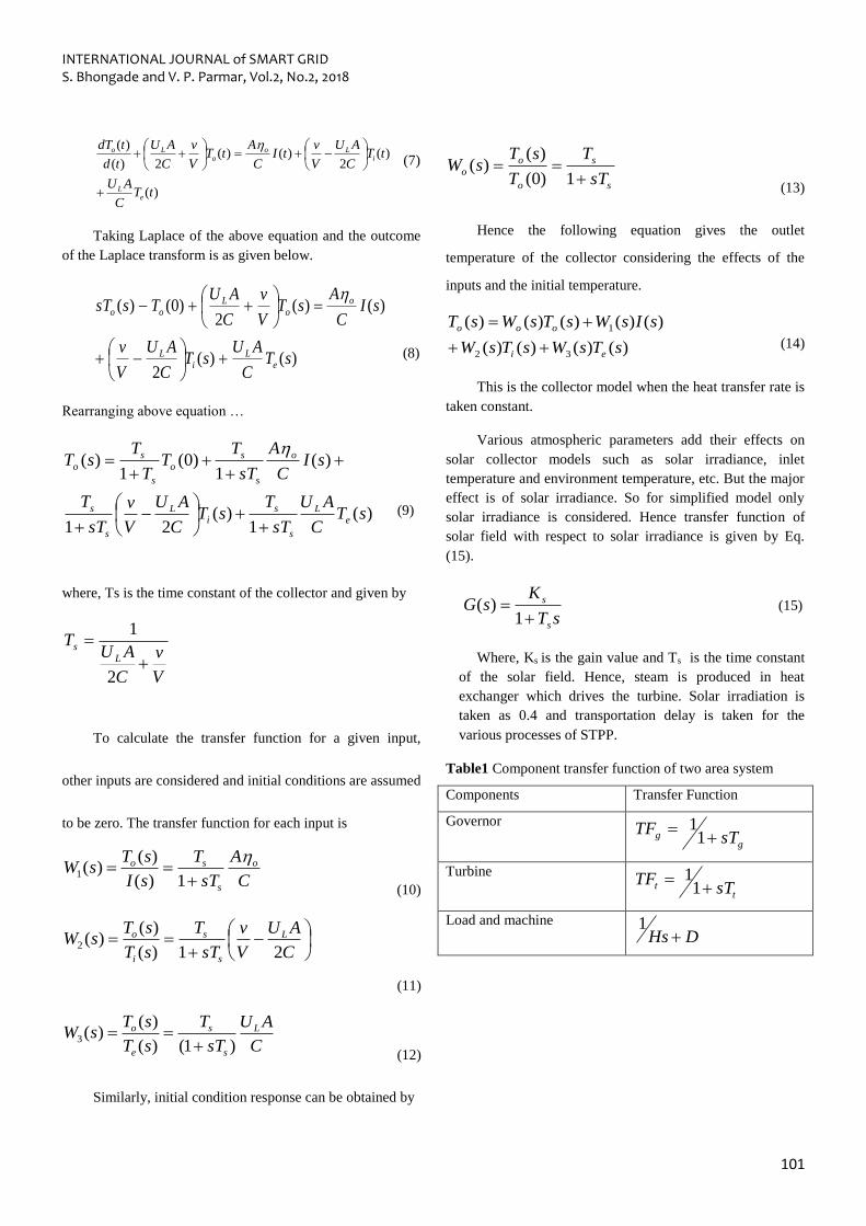
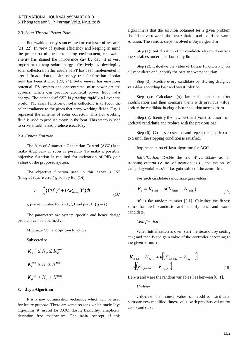
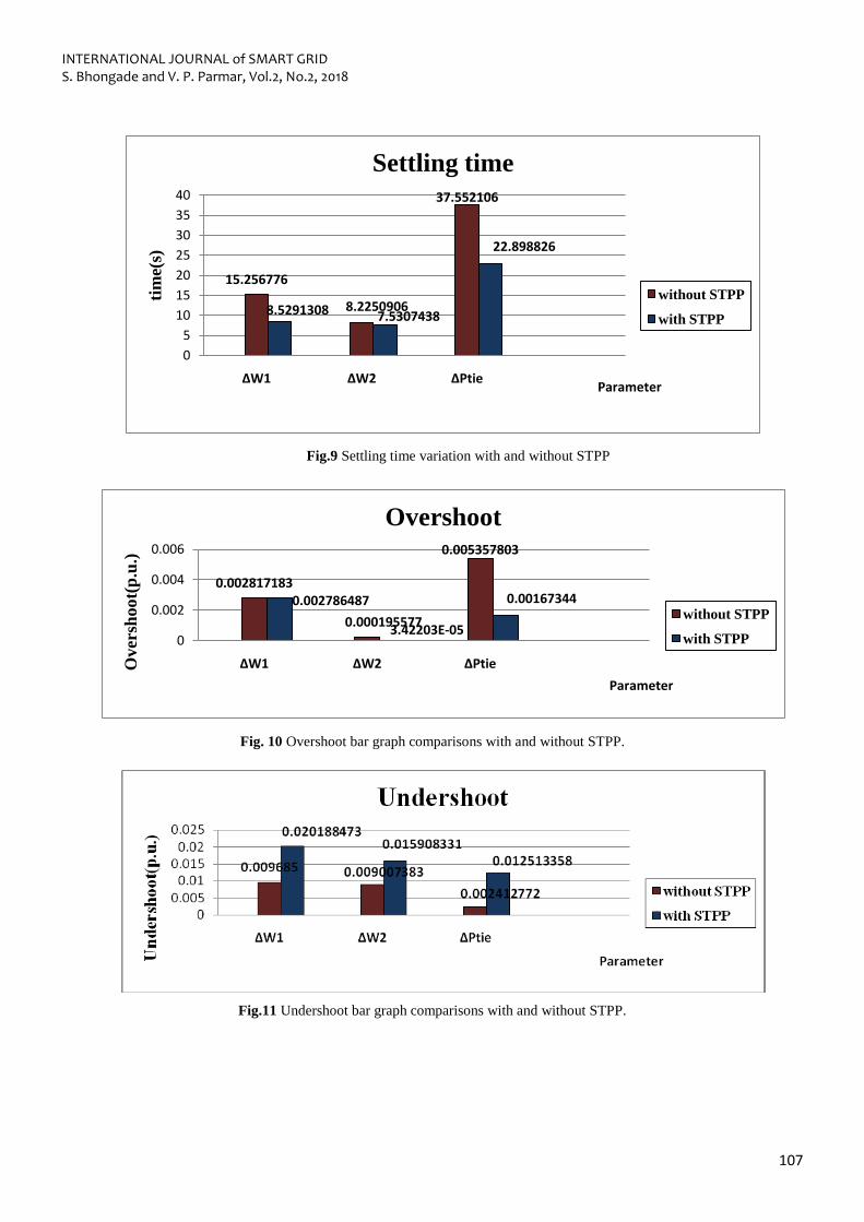
4. Simulation Results and Discussion

The dynamic performance of the proposed system is

compared with two area thermal systems at step load

perturbation of 0.2pu in both the area using Jaya algorithm.

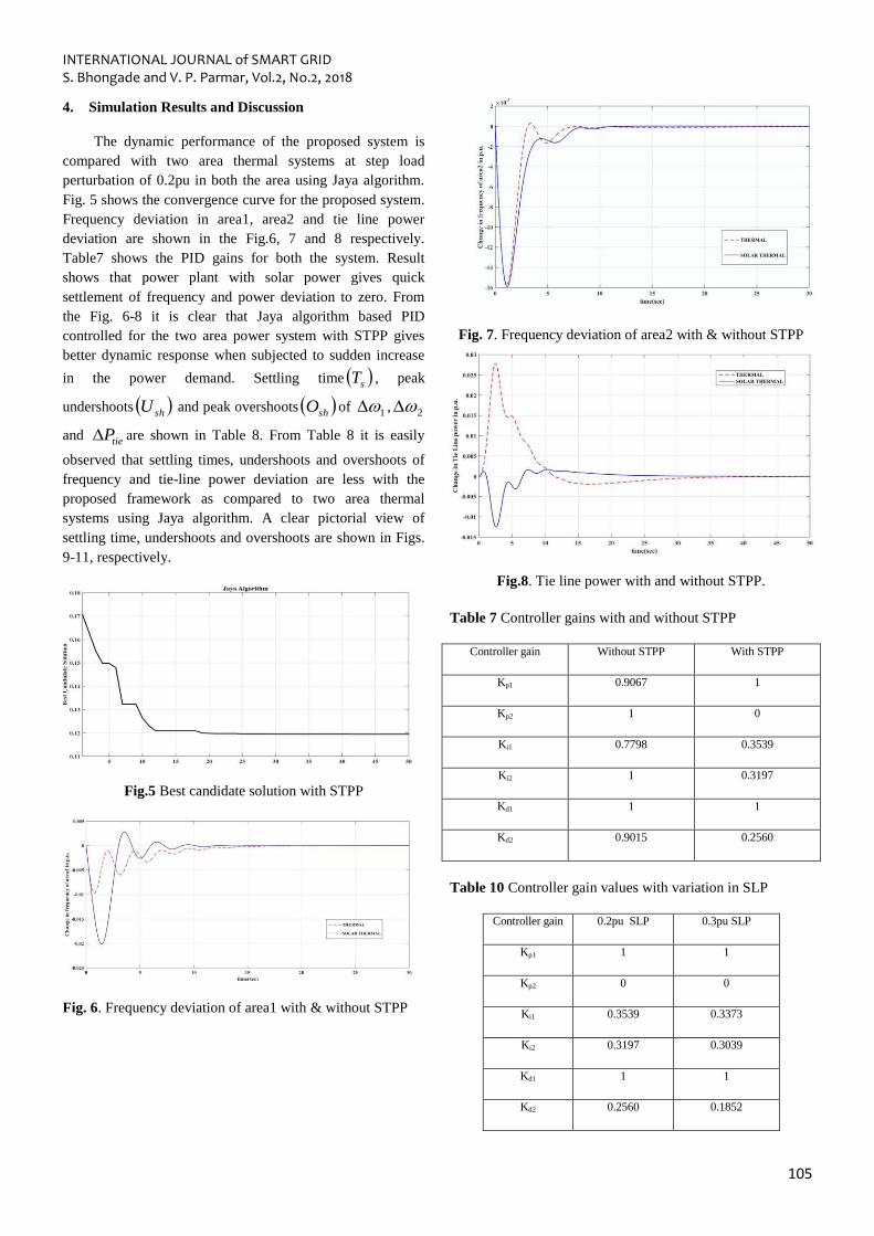
Fig. 5 shows the convergence curve for the proposed system.

Frequency deviation in area1, area2 and tie line power

deviation are shown in the Fig.6, 7 and 8 respectively.

Table7 shows the PID gains for both the system. Result

shows that power plant with solar power gives quick

settlement of frequency and power deviation to zero. From

the Fig. 6-8 it is clear that Jaya algorithm based PID

controlled for the two area power system with STPP gives

better dynamic response when subjected to sudden increase

in the power demand. Settling time sT , peak

undershoots shU and peak overshoots shO of 1 , 2

and tieP are shown in Table 8. From Table 8 it is easily

observed that settling times, undershoots and overshoots of

frequency and tie-line power deviation are less with the

proposed framework as compared to two area thermal

systems using Jaya algorithm. A clear pictorial view of

settling time, undershoots and overshoots are shown in Figs.

9-11, respectively.

Fig.5 Best candidate solution with STPP

Fig. 6. Frequency deviation of area1 with & without STPP

Fig. 7. Frequency deviation of area2 with & without STPP

Fig.8. Tie line power with and without STPP.

Table 7 Controller gains with and without STPP

Controller gain Without STPP With STPP

Kp1 0.9067 1

Kp2 1 0

Ki1 0.7798 0.3539

Ki2 1 0.3197

Kd1 1 1

Kd2 0.9015 0.2560

Table 10 Controller gain values with variation in SLP

Controller gain 0.2pu SLP 0.3pu SLP

Kp1 1 1

Kp2 0 0

Ki1 0.3539 0.3373

Ki2 0.3197 0.3039

Kd1 1 1

Kd2 0.2560 0.1852

INTERNATIONAL JOURNAL of SMART GRID S. Bhongade and V. P. Parmar, Vol.2, No.2, 2018

106

Table 8 Dynamic performance with and without STPP

Table 9 Comparison of Integra, PI controller with PID using

Jaya algorithm for STPP

Parame

ters

Dynamic performa

nce

Integral

control

PI control PID

control

∆w1

Settling

time

11.92054 14.41872

9

8.5291308

Over

shoot

0.012924

503

0.002328

1984

0.0027864

87

Under

shoot

0.025128

898

0.020845

056

0.0201884

73

∆w2

Settling

time

14.65804

7

13.97882

7

7.5307438

Over

shoot

0.002179

5308

0.001641

0739

0.0000342

2029

Under

shoot

0.018085

167

0.019666

237

0.0159083

31

∆Ptie

Settling

time

24.37099

4

31.00917

1 22.898826

Over

shoot

0.014122

517

0.004050

3251

0.0016734

4

Under

shoot

0.045736

824

0.008765

3243

0.0125133

58

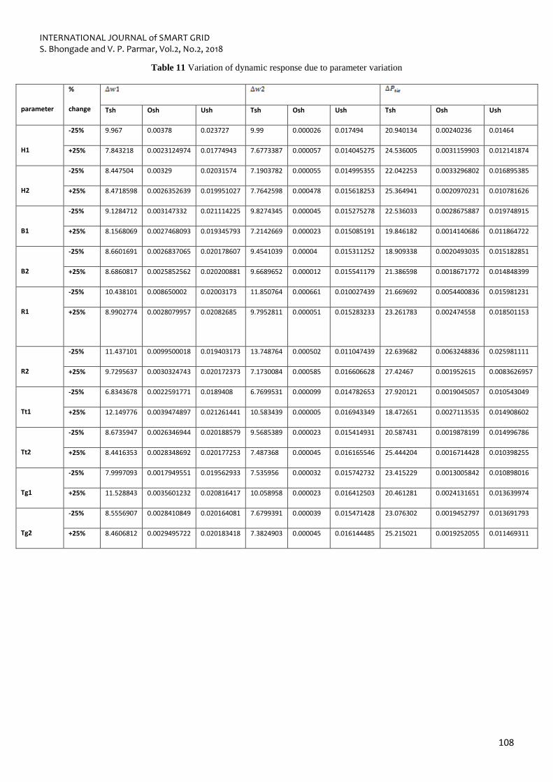
4. Sensitivity analysis

For sensitivity analysis the parameters and loading

condition of the system are changed and controller gains are

optimized using Jaya algorithm. The dynamic responses

corresponding to these changes are obtained and compared

with the result with the dynamic responses at nominal

condition. It is essential for a robust controller that response

should be more or less same and there must be no need to

reset the controller. In the present work, sensitivity analysis

is performed to confirm the robustness of the system with

STPP at nominal condition and parameters. To accomplish

the analysis, system parameter is changed from ‘-25% to

+25%’ and SLP is changed to 0.2pu and 0.3pu.For every

changed condition the Jaya algorithm is used. Table10 and

Table11 give the complete dynamic response of the proposed

system for SLP and parameter variation when sensitivity

analysis is performed. By observing the responses, it is very

clear that obtained responses more or less are same. Thus, it

is not necessary to change the gains of the PID at nominal to

large change in system parameter and system loading

condition. That means Jaya optimized PID controlled AGC

with STPP is quite robust towards variation in the system

over a wide range.

Parameters Dynamic

performanc

e

Without

STPP With STPP

∆w1

Settling

time 15.256776 8.5291308

Over shoot 0.002817183 0.00278648

7

Under

shoot

0.009684018

5

0.02018847

3

∆w2

Settling

time

8.2250906 7.5307438

Over shoot 0.000195577

12

0.00003422

029

Under

shoot

0.009007382

8

0.01590833

1

∆Ptie

Settling

time 37.552106 22.898826

Over shoot 0.005357803

3

0.00167344

Under

shoot

0.002412772

3

0.01251335

8

INTERNATIONAL JOURNAL of SMART GRID S. Bhongade and V. P. Parmar, Vol.2, No.2, 2018

107

15.256776

8.2250906

37.552106

8.5291308 7.5307438

22.898826

0

5

10

15

20

25

30

35

40

∆W1 ∆W2 ∆Ptie

tim

e(s)

Parameter

Settling time

without STPP

with STPP

Fig.9 Settling time variation with and without STPP

0.002817183

0.000195577

0.005357803

0.002786487

3.42203E-05

0.00167344

0

0.002

0.004

0.006

∆W1 ∆W2 ∆PtieOv

ersh

oo

t(p

.u.)

Parameter

Overshoot

without STPP

with STPP

Fig. 10 Overshoot bar graph comparisons with and without STPP.

Fig.11 Undershoot bar graph comparisons with and without STPP.

INTERNATIONAL JOURNAL of SMART GRID S. Bhongade and V. P. Parmar, Vol.2, No.2, 2018

108

Table 11 Variation of dynamic response due to parameter variation

parameter

%

change

Tsh Osh Ush Tsh Osh Ush Tsh Osh Ush

H1

-25% 9.967 0.00378 0.023727 9.99 0.000026 0.017494 20.940134 0.00240236 0.01464

+25% 7.843218 0.0023124974 0.01774943 7.6773387 0.000057 0.014045275 24.536005 0.0031159903 0.012141874

H2

-25% 8.447504 0.00329 0.02031574 7.1903782 0.000055 0.014995355 22.042253 0.0033296802 0.016895385

+25% 8.4718598 0.0026352639 0.019951027 7.7642598 0.000478 0.015618253 25.364941 0.0020970231 0.010781626

B1

-25% 9.1284712 0.003147332 0.021114225 9.8274345 0.000045 0.015275278 22.536033 0.0028675887 0.019748915

+25% 8.1568069 0.0027468093 0.019345793 7.2142669 0.000023 0.015085191 19.846182 0.0014140686 0.011864722

B2

-25% 8.6601691 0.0026837065 0.020178607 9.4541039 0.00004 0.015311252 18.909338 0.0020493035 0.015182851

+25% 8.6860817 0.0025852562 0.020200881 9.6689652 0.000012 0.015541179 21.386598 0.0018671772 0.014848399

R1

-25% 10.438101 0.008650002 0.02003173 11.850764 0.000661 0.010027439 21.669692 0.0054400836 0.015981231

+25% 8.9902774 0.0028079957 0.02082685 9.7952811 0.000051 0.015283233 23.261783 0.002474558 0.018501153

R2

-25% 11.437101 0.0099500018 0.019403173 13.748764 0.000502 0.011047439 22.639682 0.0063248836 0.025981111

+25% 9.7295637 0.0030324743 0.020172373 7.1730084 0.000585 0.016606628 27.42467 0.001952615 0.0083626957

Tt1

-25% 6.8343678 0.0022591771 0.0189408 6.7699531 0.000099 0.014782653 27.920121 0.0019045057 0.010543049

+25% 12.149776 0.0039474897 0.021261441 10.583439 0.000005 0.016943349 18.472651 0.0027113535 0.014908602

Tt2

-25% 8.6735947 0.0026346944 0.020188579 9.5685389 0.000023 0.015414931 20.587431 0.0019878199 0.014996786

+25% 8.4416353 0.0028348692 0.020177253 7.487368 0.000045 0.016165546 25.444204 0.0016714428 0.010398255

Tg1

-25% 7.9997093 0.0017949551 0.019562933 7.535956 0.000032 0.015742732 23.415229 0.0013005842 0.010898016

+25% 11.528843 0.0035601232 0.020816417 10.058958 0.000023 0.016412503 20.461281 0.0024131651 0.013639974

Tg2

-25% 8.5556907 0.0028410849 0.020164081 7.6799391 0.000039 0.015471428 23.076302 0.0019452797 0.013691793

+25% 8.4606812 0.0029495722 0.020183418 7.3824903 0.000045 0.016144485 25.215021 0.0019252055 0.011469311

INTERNATIONAL JOURNAL of SMART GRID S. Bhongade and V. P. Parmar, Vol.2, No.2, 2018

109

5. Conclusion

In this paper renewable energy source that is solar

thermal power plant (STPP) is incorporated with two area

automatic generation control system and also a new

optimization technique i.e. Jaya algorithm is used. It was also

concluded that after using solar power in area one, the

dynamic performance of the framework is improved

compared to without STPP. Jaya algorithm is used for the

first time in Automatic Generation Control for optimization

of several parameters such as gain value of the PID

controller. Comparison of performance of classical controller

such as integral (I), proportional integral (PI), proportional

integral derivative (PID) reveals that the PID controller gives

better result with STPP. It is also found that the dynamic

response of the system with STPP is improved from the view

point of settling time, peak overshoot, undershoot and

magnitude of the oscillations. From sensitivity analysis point

of the system, it is found that Jaya algorithm based PID

controller gains obtained at specified condition and specified

system parameters is quite robust and it is not necessary to

reset parameter for large variations in the system and other

system parameters.

References

[1] Elgerd Ol. Fosha C,”Optimal megawatt frequency

control of multi area electric energy systems”, IEEE

Trans Electric Power Apparatus System, vol.PAS-89,

pp.556-63, 1970.

[2] C. Fosha and O. I. Elgerd, “The megawatt-frequency

control problem: A new approach via optimal control

theory,” IEEE Trans. Power Apparatus & Systems, vol.

PAS-89, no. 4, pp.563–577, Apr. 1970.

[3] O.I. Elgard”Electrical Energy System Theory: An Intro,

2nd Ed”, New York: McGraw Hill, 1982. [BOOK].

[4] M. L. Kothari and J. Nanda, “Application of optimal

control strategy to automatic generation control of a

hydrothermal system”, IEE Proceedings, vol. 135, no.4,

Jul. 1988.

[5] Abido MA, “ AGC Tuning Of Interconnected Reheat

Thermal Systems With Particle Swarm Optimization”,

IEEE Trans Energy Conversion;17(3):406-13,2003.

[6] J. Nanda, A. Mangal and S. Suri, “Some New Findings

on Automatic Generation Control of an Interconnected

Hydrothermal System With Conventional Controllers”,

IEEE Trans. on Energy Conversion, vol. 21, no. 1, Mar.

2006.

[7] Gayadhar Panda, Sidhartha Panda and C. Ardil,” Hybrid

Neuro Fuzzy Approach for Automatic Generation

Control of Two –Area Interconnected Power

System”,Int J Electr Power Energy Syst;59:19–35, 2009.

[8] Saikia Lalit Chandra, Nanda J, Mishra S, “Performance

comparison of Several classical controllers in AGC for

multi-area interconnected thermal system”, Int J Electr

Power Energy Syst;33(3):394–401, 2011.

[9] Das Dulal Ch,Sinha N, Roy Ak, “GA based frequency

controller for solar thermal-diesel, wind hybrid energy

generation/energy storage system”, Int J Electr Power

Energy Syst;43(1):262-79.2012.

[10] J.Nanda, S.Mishra and L.C.Saikia, “Maiden Application

of Bacterial Foraging Based Optimization Technique in

Multiarea Automatic Generation Control”, IEEE

Transactions on Power Systems, vol. 22, No.2, pp.602-

609, 2009.

[11] Praghnesh Bhatt. Roy R. Ghoshal S.P., “GA/particle

swarm intelligence based optimization of two specific

varieties of controller devices applied to two-area multi-

units automatic generation control”, Electrical Power

and Energy Systems; 32: 299–310; 2010.

[12] H. Golpira, H. Barvani, “Application of GA

optimization for automatic generation control design in

an interconnected power system”, Energy Conversion

and Management; 52: 2247- 2255, 2011.

[13] LC Saikia. “Automatic Generation Control of a

combined cycle gas turbine plant with classical

controllers using firefly algorithm”, International Journal

of Electrical Power and Energy Systems, vol.53, pp. 27-

33, 2013.

[14] Shashi Kant Pandey, Soumya R. Mohanty, Nand Kishor

. “A literature survey on load–frequency control for

conventional and distribution generation power

systems”. Renewable and Sustainable Energy Reviews,

25:318–334, 2013.

[15] Banaja Mohanty, Sidhartha Panda , P.K. Hota,

“Controller parameters tuning of differential evolution

algorithm and its application to load frequency control

of multisource power system” , Electrical Power and

Energy Systems; 54: 77–85, 2014.

[16] Hassan A. Yousef, Khalfan AL-Kharusi, Mohammed H.

Albadi. “Load Frequency Control of a Multi-Area Power

System: An Adaptive Fuzzy Logic Approach”. IEEE

Transaction on Power System,vol.29,No. 4, Jul. 2014.

[17] Rao, R.V., Savsani, V.J. &Vakharia, D.P., “ Teaching-

learning-based optimization: A novel method for

constrained mechanical design optimization problems”.

Computer-Aide Design, 43(3), 303-315, 2011.

INTERNATIONAL JOURNAL of SMART GRID S. Bhongade and V. P. Parmar, Vol.2, No.2, 2018

110

[18] Rao RV. “Jaya: A simple and new optimization

algorithm for solving constrained and unconstrained

optimization problems”. Int J Ind Engg Comput

;7(1):19e34, 2016.

[19] R.V. Rao, D.P. Rai,Joze Balic, “A multi-objective

algorithm for optimization of modern machining

processes”. Engineering Applications of Artificial

Intelligence; 61:103–125, 2017.

[20] Binod Kumar Sahu, Swagat Pati, Pradeep Kumar

Mohanty, Sidharth Panda, “Teaching - learning based

optimization algorithm based fuzzy-PID Controller form

automatic generation control of multi-area power

System”, Int JElectr Power Energy Syst;48:19– 32,2014.

[21] Reddy VSiva, Kaushik SC, Ranjan KR, Tyagi SK.

“State-of-the-art of solar thermal power plants—a

review”. Renew Sust Energy Rev, 27:258–73, 2013.

[22] Fontalvo Armando, Garcia Jesus, Sanjuan Marco,

Vasquez Padilla Ricardo. “ Automatic control strategies

for hybrid solar-fossil fuel power plants”. Renewable

Energy; 62:424– 31, 2014.

[23] Buz´as J, Kicsiny R,“Transfer functions of solar

collectors for dynamical analysis and control design”,

Renewable Energy;68:146–55, 2014.

[24] Yatin Sharma, Lalit Chandra Saikia. “Automatic

generation control of multi- area STThermal power

system using Grey Wolf Optimizer algorithm based

classical controllers”. Electrical Power and Energy

Systems; 73,853–862,2015.

[25] Jagatheesan K., Anand B., Baskaran K., Dey N., Ashour

A., Balas V. (2018) Effect of Nonlinearity and Boiler

Dynamics in Automatic Generation Control of Multi-

area Thermal Power System with Proportional-Integral-

Derivative and Ant Colony Optimization Technique. In:

Kyamakya K., Mathis W., Stoop R., Chedjou J., Li Z.

(eds) Recent Advances in Nonlinear Dynamics and

Synchronization. Studies in Systems, Decision and

Control, vol 109. Springer, Cham.

[26] SasmitaPadhy,SidharthaPanda, “A hybrid stochastic

fractal search and pattern search technique based

cascade PI-PD controller for automatic generation

control of multi-source power systems in presence of

plug in electric vehicles”, CAAI Transactions on

Intelligence Technology, Volume 2, Issue 1, March

2017, Pages 12-25.

[27] Tapabrata Chakraborty ; David Watson ; Marianne

Rodgers , “Automatic Generation Control Using an

Energy Storage System in a Wind Park”, IEEE

Transactions on Power Systems, Vol. 33, No. 1, January

2018.

[28] M. Del Castillo, G. P. Lim, Y. Yoon, and B. Chang,

“Application of frequency regulation control on the 4

MW/8 MWh battery energy storage system (BESS) in

Jeju Island, Republic of Korea,” J. Energy Power

Sources, vol. 1, no. 6, pp. 287–295, 2014.

[29] Lei Zhang ; Yi Luo 1 ; Jing Ye ; Ya-yuan Xiao ,

“Distributed coordination regulation marginal cost

control strategy for automatic generation control of

interconnected power system”, IET Generation,

Transmission & Distribution , Volume 11, Issue 6 , 20

April 2017, p. 1337 – 1344.

[30] Satya Dinesh Madasu, M.L.S. Sai Kumar, Arun Kumar

Singh, Comparable Investigation of Backtracking Search

Algorithm in Automatic Generation Control for Two

Area Reheat Interconnected Thermal Power System,

(2017), http://dx.doi.org/10.1016/j.asoc.2017.01.018.

[31] Debdeep Saha and Lalit Chandra Saikia , “Automatic

generation control of a multi-area CCGT-thermal power

system using stochastic search optimised integral minus

proportional derivative controller under restructured

environment”, IET Generation, Transmission &

Distribution, Volume 11, Issue 15 , 19 October

2017, p. 3801 – 381.

[32] Arya, Y., Kumar, N.: ‘AGC of a multi-area multi-source

hydrothermal power system interconnected via AC/DC

parallel links under deregulated environment’, Int. J.

Electric. Power Energy Syst., 2016, Vol 75, pp. 127–

138.