Automatic Fume Hood Sash Closure - Home | High … · 2017-09-20 · B. Genome Building Lab 1010 ... Debbie Decker, Campus Chemical Safety Officer, EH&S ... Automatic Fume Hood Sash

Pacific Gas and Electric Company

Emerging Technologies Program

Application Assessment Report 0607

Automatic Fume Hood Sash Closure Demonstration and Test at:

The University of California, Davis

Issued: November 5, 2007 Project Manager: Alicia Breen, Francois Rongere Pacific Gas and Electric Company Prepared By: Lawrence Berkeley National Laboratory and Cogent Energy, Inc.

LEGAL NOTICE This report was prepared by Pacific Gas and Electric Company for exclusive use by its employees and agents. Neither Pacific Gas and Electric Company nor any of its employees andagents: (1) makes any written or oral warranty, expressed or implied, including, but not limited to those

concerning merchantability or fitness for a particular purpose; (2) assumes any legal liability or responsibility for the accuracy, completeness, or usefulness of

any information, apparatus, product, process, method, or policy contained herein; or (3) represents that its use would not infringe any privately owned rights, including, but not

limited to, patents, trademarks, or copyrights.

1

Contents

I. ACKNOWLEDGEMENTS..............................................................................3

II. EXECUTIVE SUMMARY ...............................................................................4

III. BACKGROUND .........................................................................................7

A. Introduction..............................................................................................................7 B. End State Goal .........................................................................................................7 C. Fume Hood Energy Consumption and Potential Savings........................................8 D. Fume Hood Energy Efficiency ................................................................................9 E. Automatic Sash Closure.........................................................................................18

IV. OBJECTIVES...........................................................................................19

V. DEMONSTRATION DESIGN AND PROCEDURES....................................19

VI. HOST SITE ..............................................................................................20

A. Plant and Environmental Sciences (PES) Lab 1247 ..............................................20 B. Genome Building Lab 1010...................................................................................23

VII. RESULTS.................................................................................................24

A. Energy and Demand Savings .................................................................................24 B. Limitations .............................................................................................................43 C. Sensitivity Analysis ...............................................................................................44 D. Economic Analysis ................................................................................................47 E. Issues Encountered.................................................................................................49 F. Feasibility for wide-spread implementation ..........................................................50 G. Market size and potential .......................................................................................50

VIII. CONCLUSIONS.......................................................................................52

IX. RECOMMENDATIONS FOR FUTURE WORK........................................55

X. APPENDICES..............................................................................................56

A. Monitoring and Evaluation Plans...........................................................................57 B. PG&E Brochure .....................................................................................................60 C. Test Site Solicitation and Requirements ................................................................62 D. Power Point Presentation .......................................................................................65 E. Report to Campus ..................................................................................................77

2

I. Acknowledgements The primary authors if this report were: Dale Sartor, Lawrence Berkeley National Laboratory Rishabh Kasliwal, Cogent Energy, Inc. The authors would like to thank: From Cogent Energy, Inc.:

Michael Daukoru Doug Chamberlin

From UC Davis:

Mark Anthony Nicholas Mark D Nicholas Dave Henderson Debbie Decker, Campus Chemical Safety Officer, EH&S Elaine Bose, Safety Coordinator, Department of Plant Sciences

From PG&E:

Alicia Breen Francois Rongere

From Lab Specialists:

David Sweitzer

3

II. Executive Summary Fume hoods contribute to approximately 2,495 GWh/year, 574 MW, and 18 Trillion BTUs/year in California. Assuming one third the hoods are in the PG&E territory (28,000 hoods), their estimated energy requirement is 800 GWh/year, 190 MW, and 60 million therms. The end-state goal is to reduce airflow through fume hoods by 75%. This goal will be accomplished through multiple technology options including:

• Reduce the number and size of fume hoods • Restrict the sash opening • Two “speed” occupied and un-occupied • Variable Air Volume (VAV) • High Performance Hoods

This study focuses on a variation of two “speed” occupied and un-occupied, and variable air volume (VAV) by installing an automatic sash closure system on a VAV hood that is controlled by an occupancy sensor. This technology has the potential to meet the end state goal of saving 75% Demonstration automatic fume hood sash closure systems were installed in two laboratories at UC Davis. A summary of the results are presented in Table 1 – Annual Savings per CFM, Table 2 – Savings per Hood, and Table 3 – Demand Savings.

Table 1 Automatic Fume Hood Sash Closure Annual Savings per CFM

(Energy and Dollars)

Configuration PES Genome Therms KWh $ Therms KWh $ 1. Gas cooled 2.5 4.0 $2.39 3.0 9.2 $3.16 2. Electric cooled 2.1 5.8 $2.17 2.0 13 2.56 3. Electric w/ normal 55

deg. F supply (PES only) 1.9 9.2 $2.25

4. Same as #3 w/ commercial PG&E rates

1.9 9.2 $3.44 2.0 13 3.90

4

Table 2

Savings Per Hood Assuming Typical Configuration and Utility Rates (CFM and Dollar)

Configuration PES (6 ft. Hood) Genome (5 ft.

Hood) CFM $ CFM $ 1. Base (“Typical”) 533 $1834 293 $1143 2. Hood driven load (all savings captured) 533 $1834 433 $1689 3. Remove sash stops and assume CAV

(or open VAV) - most energy intensive scenario

1333 $4586 866 $3377

Base (typical conditions) is configuration #4 in Table 1

Table 3 Demand Savings

Per CFM Per Hood

(533 cfm PES and 433 cfm Genome)

PES gas cooled 1.6 W .9 kW PES electric chiller 3.5 W 1.9 kW Genome gas cooled 2.3 W 1 kW Genome electric cooled 4.8 W 2.1 kW Cost Effectiveness At a cost of $4,500 per hood, the simple payback is 1 to 4 years based on the two test conditions and PG&E commercial rates. 2.3 to 2.5 year payback would be typical for a hood driven load. Low utility rates and other unique conditions at UC Davis yielded a lower unit savings and a longer payback. While the energy savings and cost effectiveness is attractive in retrofit, there could be even greater advantages in new construction. If the automatic fume hood sash closure system is deployed in new construction, and the design team assumes a small fraction of the hoods are simultaneously open, the reduced infrastructure size and cost (fans, ducts, boilers, chillers, etc.) can offset the increased hood control cost.

5

CO2 Savings Assuming 1.1 lbs/kWh and 11.7 lbs/therm and the base case (typical conditions), the annual CO2 savings, is estimated as: Per CFM Per Hood PES (533 cfm) 32 lbs 17K lbs Genome (433 cfm) 37 lbs 16K lbs

6

III. Background

A. Introduction Exhaust hoods protect operators from breathing harmful fumes by capturing, containing, and exhausting hazardous gases created in laboratory experiments or industrial processes. These box-like structures, often mounted at tabletop level, offer users protection with a movable, window-like front “face” called a sash. Fans draw fumes out the tops of the hoods.

Standard fume hood in use.

Fume hood exhaust induces airflow through the fume hood’s “face.” The generally accepted “face velocity” is 100 feet/minute; a high airflow rate causing large exhaust flows. Interestingly, increasing face velocity does not necessarily improve containment. Instead, errant eddy currents and vortexes can be induced around hood users as air flows into the hood, reducing containment effectiveness. Fume hoods exhaust large volumes of air at great expense. The energy to filter, move, cool, heat or reheat, and in some cases scrub (clean) this air is one of the largest loads in most lab facilities. Fume hoods frequently operate 24 hours/day. Since many laboratories have multiple hoods, they often dictate a lab’s required airflow and thus the supply and exhaust systems’ capacity. The result is larger fans, chillers, boilers, and ducts compared to systems having less exhaust. Consequently, fume hoods are a major factor in making a typical laboratory four to five times more energy intensive than a typical commercial space. Most state-of-the-art, energy-efficient fume hood systems require several interactive features and diligent users. Sophisticated controls, for each hood and for supply and exhaust air streams combine to provide the recommended face velocity and pressure differential between the laboratory and adjacent space.

B. End State Goal The end state goal in reducing the energy impact of California fume hoods is a 75% reduction in airflow (NFPA minimum flow requirements for dilution) while maintaining or improving safety.

7

C. Fume Hood Energy Consumption and Potential Savings A six-foot-wide hood typically exhausts 1250 cubic feet per minute (cfm), 24 hours per day, consuming three-times more energy than an average house. Greenhouse-gas emission caused by operating the typical hood is equivalent to six automobiles.

Fume Hood Energy Consumption

Using calc.htThis w

Califogoal is

1.

2.

=

the fume hood calculator developed by LBNL (available at http://hightech.lbl.gov/fh-ml) an estimate of California fume hood energy use (gas, electric, and peak) follows. as based on the assumption of an equivalent of 85,000 1250 cfm fume hoods installed.

Electricity GWh/year: 2,495 Total Peak Power MW: 574 Total Natural Gas Trillions BTUs/year: 18

rnia ratepayers are spending over $400 million to operate their fume hoods. While the to reduce fume hood airflow 75%, energy savings will be different:

Two thirds of the KWh and one third of the KW savings are from the fans. In a static system, fan energy reduces at approximately the cube of the flow. Therefore a 75% reduction in fume hood flow can result in more energy savings, especially in the main supply fans which provide air for other purposes than the hoods (the impact will be at the margin where flow reductions will have the greatest impact). However as will be seen in this case study, more sophisticated controls will be required to achieve this potential. Fume hoods don’t always “drive” the required air change rate. In labs with few hoods, other factors such as the minimum air change rate and thermal loads can

8

http://hightech.lbl.gov/fh-calc.html

http://hightech.lbl.gov/fh-calc.html

dictate the required airflow. In these situations, reductions of airflow through the fume hoods are “made-up” by increases in the general room exhaust.

We are assuming that 1 and 2 cancel each other out for electricity, and therefore assume that the end state goal will result in a 75% electrical savings. We assume that the savings for natural gas is discounted 20% (of 75%) to yield a 60% potential savings:

Saved Electricity GWh/year: 1,871 Saved Peak Power MW: 431 Saved Natural Gas Trillions BTUs/year: 11

D. Fume Hood Energy Efficiency The end goal will be achieved through multiple technology options:

1. Reduce the number and size of fume hoods 2. Restrict the sash opening 3. Auxiliary air hoods 4. Two “speed” occupied and un-occupied 5. Variable Air Volume (VAV) 6. High Performance Hoods

9

1. Reduce the number and size of fume hoods

New labs often standardize on a single hood size (increasingly larger) and install more than needed to allow for growth and flexibility (for example two per lab module). Existing labs often have rooms needing hoods (one of the reasons new labs get so many), while many other rooms have underutilized hoods. It is best to:

o Size distribution for ample capacity but install only hoods needed immediately o Provide tees, valves, and pressure controls for easy additions and subtractions o Encourage removal of underutilized hoods (some labs are going to hoods as a

shared resource)

Is this hood intensity necessary?

10

2. Restrict the sash opening

In an effort to maintain 100 fpm face velocity, fume hood designs have been developed to simply reduce/restrict the sash opening and thus save air/energy. The two most popular techniques are horizontal sliding sashes and sash stops.

a. Horizontal sliding sashes Horizontal sliding sashes are used to restrict the fume hood opening and protect the user. In theory these sliding sashes cannot be opened all the way but two (or more) can overlap, creating an opening. Some users feel the sashes get in the way and remove them (not a safe or efficient option). Further the sashes’ sharp edges can cause turbulence, reducing the ability of the hood to contain. Some companies, with strong sash management cultures, have successfully used this technique.

• Horizontal Sash

Sash Panels

Opening–Can be more energy efficient due to reduce airflow volume

–May increase worker safety

–Caution – sash panels can be removed; defeats safety

11

b. Sash stops Sash stops prevent the sash from opening all the way. Usually the stops are placed at 18” thus blocking the top two fifths of the opening. In most cases the stops are designed for easy override to lift the sash out of the way during setup. Systems designed for the 18” opening violate Cal/OSHA standards when the sash stops are bypassed. A corporate culture that assures bypass only when hazards are not present is needed. Sash stops “encourage” diversity in VAV hoods (at least the hood is partially closed – 2/5ths or more – most of the time).

• Vertical Sash Opening

3. Auxil Auxiliaboveenergypopulathan aair hoo

– Most common sash

– Good horizontal access

– Energy use reduced with sash stop

Vertical Sash Stop

iary air hoods

ary air hoods bring tempered make-up air directly to the hoods and introduce it the sash (above the users head). These hoods were introduced in the 1970’s for efficiency. They are still shown in manufacturers’ catalogs, however their rity has waned due to comfort and safety issues. Energy savings has been less

nticipated as the “tempered” air is conditioned to provide comfort. Auxiliary ds are not recommended.

12

• Auxiliary Air Hood– Wastes energy

– Reduces containment performance

– Decreases worker comfort

– Disrupts lab temperature and humidity

– Not Recommended

4. Two “speed” occupied and un-occupied In theory, a hood that is unoccupied doesn’t need the same airflow than one with a person at or near its face. Control companies offer an occupancy sensor based two-position control that reduces the face velocity from 100 fpm to around 60 fpm unoccupied. These systems are sometimes marketed as a “substitute” for VAV but they could be combined with VAV and other technologies. There benefit is assured savings even when the fume hood sash is left open. Therefore, in an environment of poor sash management, they can save more energy than VAV. Cal/OSHA has recently approved this technology (with conditions such as tracer gas testing) for use in California.

Two speed control with occupancy sensor range

13

5. Variable Air Volume (VAV)

VAV fume hood systems control the airflow to maintain a constant face velocity. As the sash is closed, the exhaust air volume is automatically decreased. In a VAV system, energy savings occur when a hood’s sash is less than fully open, which reduces exhaust flow while maintaining a constant face velocity. Each hood user must operate the sash properly to ensure that the system achieves full energy savings potential.

The VAVair pressuassumptioassume alup to a 50assumed w Since its iconstructiof the potpotential s The biggewide opensynergisti

exhaust must be coupled with a VAV supply system to maintain required re relationships in labs. “Rightsizing” the HVAC system requires an n regarding the diversity of the sashes. The most conservative designers l the hoods are open when sizing their equipment. Other designers assume % (closed) diversity depending on the number of hoods (greater diversity is ith larger numbers).

ntroduction in the 1980’s, VAV has grown to a large market share in new on. Assuming 30% of the hoods installed in California have VAV and 50% ential end state savings is achieved, VAV has already captured 15% of the avings outlined above.

st problem with VAV is no energy is saved if the fume hood sashes are left . Therefore, the savings depends on the users. Energy and safety goals are

c with VAV hoods – a closed hood is much safer than an open hood.

VAV Hood Operation

14

a. Sash management

Any effort to encourage sashes being closed is called sash management. This can include: signs, pamphlets, training, incentives (e.g. monetary awards when spot checks find sashes closed), and penalties (e.g. monitoring systems that can provide information to back-charge users for individual fume hood use). A study at Duke University showed user training improved sash management by over 30% (from 5% of the time closed to 39% of the time closed).

b. Demand responsive sash management (unutilized technique) Using a variety of notification systems (PA, e-mail, and telephone) this sash management technique would alert users to peak conditions and request closure of fume hood sashes. Users would be provided feedback via a graphical web site that shows reduction in energy, demand, and cost resulting from their action. A large potential savings in peak cooling will occur as reductions in outside air will occur at peak outside air temperature conditions. Also supply and exhaust fan savings can approach a cubed function (small reduction in flow yields large reduction in energy). This technique was demonstrated in another PG&E Emerging Technology project.

c. Occupied and unoccupied set points The two “speed” technology described above can be applied to VAV such that the velocity set point can be reset when the hood is “unoccupied.” Savings would accrue as a result of both the hood being unoccupied as well as the sash being closed or partially closed.

d. Auto sash closure systems Auto sash closure systems are a form of sash management, and are the focus of this study. See the next section for more details.

15

6. High Performance Hoods

e. First generation (20 to 40% savings) Several high performance hoods (safe and low flow) are on the market (outside of California). They offer advantage (over VAV) of simplicity (generally constant volume), lower peak requirements, safety, and the ability to downsize the mechanical/electrical systems (no diversity assumptions required). There is a major institutional barrier to high performance hoods in California where Cal/OSHA requires hoods to have 100 ft/min face velocity.

High performance fume hoods by Air Sentry and Labconco (representative)

16

b. Second generation (40 to 75% savings) Second generation high performance fume hoods are similar to the first generation, but with lower flow requirements to provide the same level of safety. The “Berkeley Hood” is the only known second generation high performance hood under development. While it may be possible to reach the end state goal solely with a second generation high performance hood, it may be easier (technically and from a cost standpoint) to achieve the goal with a hybrid hood system (combining high performance with control options).

Berkeley Hood by LBNL– Air Divider Technique

– Perimeter Air Supply

– Perforated Rear Baffle

– Slot Exhaust

– Optimized Upper Chamber

– Designed to minimize escape by reducing reverse flow

17

E. Automatic Sash Closure

1. Description of technology In response to poor sash management, several companies have introduced automated sash closure systems. An auto sash closure system coupled with a VAV or two position fume hood control system will come very close to meeting the end state goals since most hoods are “occupied” only a few hours a week. Much higher diversity assumptions could be made with such a system, potentially reducing first cost.

Activation Buttons

Presence Sensor

Safety Eye

The New-Tech Automatic Sash Positioning System

18

2. Market Status Market penetration of fume hood automatic sash closure systems has been slow, especially in California. Reports of problems in early installations (i.e. 1980’s) have reinforced general concerns about the technology (e.g. what if it closes or opens when you don’t want it to). There were no known operating installations in California in 2005 (an abandoned installation exists at UC Berkeley). However the current state-of-the-art seems to have overcome these barriers and concerns, and the technology is being actively marketed in California. Enhancements to the technology include:

• Pneumatic sash positioning allows one finger override (up or down) • Fails in any desired position • Safety eye stops sash closure before it hits any protrusion • Opens on presence or activation of buttons (user option) • Option for multiple sash opening selector • Advanced presence sensor technology • Selectable time delay prior to sash closing • Monitoring options

3. Related work (SCE and UCI) In addition to this demonstration/test at UC Davis, the technology is being tested at UC Irvine and at Amgen in the Southern California Edison service area. In both cases the technology has been well received.

IV. Objectives The objective of this project was to demonstrate and evaluate the opportunity for energy and demand savings in laboratories based on an automated fume hood closure system. The demonstration involved the retrofit of two existing VAV controlled fume hood in a laboratory where the fume hoods drive the outside air requirements most of the time. This project will:

• Demonstrate and evaluate emerging technology • Document baseline and post retrofit conditions to assess savings • Estimate actual energy and demand impact • Demonstrate operator acceptance of the automatic sash closure system • Promote the project and use of auto-closure fume hoods (subject to positive test

results)

V. Demonstration Design and Procedures A draft monitoring and evaluation plan was prepared by LBNL dated October 9, 2006 (see appendix). Site requirements and selection criteria were also developed (see appendix) that called for:

1. PG&E Customer

19

2. Customer willing to share performance information 3. Customer willing to cost share 4. Existing VAV fume hood and room pressure control system 5. Hood driven load 6. Poor existing sash management (based on visual inspection and interview(s)) 7. Low hazard lab with no obvious safety hazards or operational concerns 8. Easily monitored system 9. Easily accessible

UC Davis was selected as the demonstration site and a kick off meeting was held on March 5, 2007. A final monitoring and evaluation plan was prepared by Cogent Energy dated June 11, 2007 (see appendix). The plan generally followed the draft plan and provided details on the demonstration facilities, the M&E approach, sources of expected energy and demand reductions, monitoring equipment to be used, M&E procedures, and trending (monitoring) points.

VI. Host Site

A. Plant and Environmental Sciences (PES) Lab 1247 Laboratory 1247 is in an area served by one air handler (AHU-4), two exhaust fans (EF-7 and EF-8), and forty four (44) associated terminal units. It is 11 x 32 feet (350 sqft) and contains one six foot hood.

Exterior of the Plant and Environmental Sciences Lab

20

PES Demo hood prior to retrofit

PES hood prior to retrofit with hose that would not allow sash to close

21

Existing PES hood with VAV control PES Demo hood prior to retrofit (Note sash (indicating 105 fpm) stop restricts sash opening more than 50%)

Demonstration Fume Hood in PES 1247 (after installation)

22

B. Genome Building Lab 1010 Laboratory 1010 is an area in the Genome Building served by one air handler (AHU-4), an exhaust fan (EF-2), and thirty eight (38) associated terminal units. It is 21 x 39 feet (820 sqft) and contains one five foot hood.

Exterior of Genome Building

Demonstration Fume Hood in Genome Building Lab 1010

23

VII. Results

A. Energy and Demand Savings Field measurements were taken for:

• Supply air temperature and reheat temperature • Sash position or fume hood exhaust • Supply and exhaust air volume to/from the lab (and hood) • Power and air volume (cfm) of the air handler units (AHUs) • Power of associated exhaust fans

See measurement and evaluation (M&E) plan for details of field measurements. Data from short term monitoring was used in an energy model to estimate annual energy use before and after retrofit and estimate energy savings. Assumptions relating to the energy use have been documented in the M&E Plan included in the Appendix.

1. Key assumptions used: • Chilled water system (including distribution) efficiency: 1 kW/ton for electric driven

chillers, and .15 Therms/ton for gas driven chillers plus .4 kW/ton for auxiliary electric needs.

• Heating system (including distribution) efficiency: 70% • Minimum hood air flow is the equivalent of a 6” sash opening allowing for 25 cfm

per square foot (NFPA minimum) for a 24” deep interior • Sash stops were placed at 18” thus allowing for a potential savings over a 12” sash

travel • The six foot hood in PES has a 5’4” by 36” (max) sash opening, and the five foot

hood in Genome has a 4’4” by 30” (max) sash opening • Combining the above three assumptions:

Airflow in cfm

(at 100 ft/min velocity) PES Genome Nominal (max.) 1600 1083 Design (18” sash stop) 800 650 Minimum (NFPA) 267 217 Savings with 12” sash movement 533 433

• Exhaust fan power savings was considered negligible as the fans are constant volume

(with bypass at the roof) to maintain constant discharge velocities • Heating degree hours (based on 63 deg. F supply): 72,000 (compared to 32,000 with

a 55 deg. F supply) • Cooling ton hours (based on 63 deg. F supply): 3 tons/cfm (compared to 6.4 tons/cfm

at 55 deg. F supply)

24

• Utility costs:

UC Davis PG&E

Commercial Electricity blended per kWh $.066 $.10 Gas per therm $.85 $1.30

• Key assumptions based on field measurements:

PES Genome Hood cfm savings 402 (inc. to 533)1 293 (inc. to 433)2

Supply air temperature deg. F 63 55 Re-heat temperature deg. F 74 (reduce to 70)3 66.2 Supply fan Watts/cfm .32 .75

1 PES measured savings of 402 cfm (average) was with reheat valve stuck contributing to increased flow to maintain room temperature. Assume savings will increase to 533 cfm with valve fixed and hood minimum flow adjusted per prior table. 2 Genome measured savings of 293 cfm constrained by minimum room ventilation (large lab space with only one hood). Had the labs airflow been hood driven, the savings is assumed to be 433 cfm per prior table. 3 PES reheat supply temperature is high because of a leaking valve. Assume reduced to 70 deg. F when valve fixed.

25

2. Plant and Environmental Sciences (PES) Lab #1247 Supply and reheat temperatures:

The average supply air temperature was approximately 63 deg. F and remained reasonably constant. Likewise the reheat temperature was approximately 74 deg. F and was also constant. Therefore, the level of reheat was approximately 11 degrees. Note, this is an excessive level of reheat, and it appears that the reheat valve is leaking (allowing bypass of undesirable heating water).

26

Sash Position:

The pre-retrofit sash position at PES was constant at 18.” The fume hood was rarely closed and the stop was never bypassed. This hood has a tall sash so that the stop was providing a significant efficiency benefit – reducing the nominal hood design air flow approximately 50%. Therefore the sash stop provided 60% of the potential savings (as the hood must have a minimum air flow even with the sash closed). The post retrofit sash position is almost always closed. It is used two days in the average week. Note the above graph illustrates an average opening over an extended period of time. In reality the sash is opened much more for a short period of time and closes between uses. This graph better illustrates the consequences of hood use. The hood is at or near the minimum (NFPA) flow almost all the time. Therefore, the previously described end state goal is met. Air flow saved by sash stop: 50% Air flow saved by auto closure: 33.3% Minimum air flow: 16.7% Had sash stops not been deployed on this hood the savings attributed to the auto closure system would have been significantly more (83% if deployed on a constant volume hood). Had there been better sash management of the hood such that the existing VAV system was better utilized, the savings attributed to the auto closure system would have been less.

27

Supply Fan Power:

The supply fan power and air flow was monitored over its normal operational range. While the watts per cfm is actually a curve, the tangent of that curve (linear fit of operating points) in the operating range yields a slope of only .32 watts per cfm. The average (system) watts per cfm is .73, more than twice the savings in the operating range. At higher air flows the curve gets steeper and the watts per cfm would dramatically increase. One reason for the lack of savings at the margin is the supply system operates at a constant pressure. Instead of a cubed function, it is closer to linear. It may be possible to significantly improve the savings by implementing a pressure reset strategy – as the flow rate through the system decreases; the static pressure set point is also decreased, significantly reducing the load on the fan.

28

Lab Air Flow Rates Before and After Retrofit:

The air flow rates (supply and exhaust) were reasonably stable before the retrofit. The short duration of fume hood use is only because that was the period of time the hood was tested, not that it had zero flow most of the time (see sash position graph). The post retrofit data is spiky representing increases in general exhaust and supply air in an attempt to cool the space with 74 deg. F air. Once the reheat valve is fixed and the supply air temperature is reduced, the air flow should stabilize at the minimum air flow. Note the post retrofit fume hood spikes represent the few times that the hood is used.

29

Average Air Flow Rates Before and After Retrofit:

This graph of average airflow rates smoothes out the data making it easier to see the savings. Airflow at the AHU displays some time of day and time of week fluctuation, but note the axis starts at 30K cfm; the AHU operates in a relatively tight range of 34K to 37K cfm. Prior to the retrofit, the air flow into the lab of constant 74 deg. F air was reasonably constant. After the retrofit (reduction of airflow by approximately 50%) the system has a difficult time maintaining comfort with a supply temperature of 74 deg. F, so the air flow increases to accommodate modest cooling loads. This reduced the average savings to 402 cfm. Once the leaking reheat valve is fixed, the supply air flow to the lab should stabilize at less than 400 cfm (room size is 350 sqft and minimum hood flow is approximately 217 cfm – room size governs).

30

Energy and Demand Savings:

1. Airflow reduction: a. Before reheat fixed: PES is a six foot hood (approximate 64” opening).

Measured savings was 402 cfm, however as noted the potential savings was not realized do to a leaking reheat valve causing a demand for excessive airflow.

b. After reheat fixed: Savings based on 12” of closure and corresponding control (last 6” used to satisfy minimum flow) yields 533 cfm (Reduced flow = 100fpm x 5.33ft x 1ft = 533 cfm). Given that the reheat is/was always on, assume capture of the full cfm savings all the time (once the reheat control is fixed). Any reduction in total exhaust has a corresponding reduction is supply (assumes no infiltration from the exterior of the building into the lab).

2. Reheat: a. Prior to reheat repair: 11 deg F prior to reheat repair, then (11deg x

.018btu/deg/cf x 60min x 8760 hrs/year) / (.7eff x 100,000btu/therm) = 1.49 therms/cfm.

b. After reheat repair: Assume average reheat reduced to 7 deg F: (7deg x .018btu/deg/cf x 60min x 8760 hrs/year) / (.7eff x 100,000btu/therm) = 0.95 therms/cfm.

3. Heat outdoor air to 63 deg F. Assume 72,000 heating degree hours. This is conservative as 100% outside air requires heat at night even when the average temperature is “neutral.” Saves: 72,000deghrs x .018btu/deg/cf x 60min) / (.7eff x 100,000btu/therm) = 1.11 therms/cfm

4. Gas cooling: Assume 3 tons/cfm and .15 therms/ton, then .45 therms/cfm 5. Total annual gas savings:

a. Before reheat fixed = 1.49 + 1.11 + .45 = 3.1 therms/cfm (2.6 w/o gas cool) b. After reheat fixed = .95 + 1.11 + .45 = 2.5 therms/cfm (2.1 w/o gas cool)

6. Saving at $.85/therm: a. Before reheat fixed = $2.64/cfm ($2.21 w/o gas cool) b. After reheat fixed = $2.13/cfm ($1.79 w/o gas cool)

7. Fan power: .32 W/cfm, then .32 W/cfm x 8760hrs/1000W = 2.8 kWh/cfm 8. Electric power w/ gas cooling: Assume 3 ton-hours/cfm and .4 kW/ton then

1.2kWh/cfm 9. Total annual electric kWh/cfm with gas cooling: 2.8 + 1.2 = 4 kWh/cfm 10. Savings at $.066/kWh: $.26/cfm 11. Total savings per cfm with gas cooling

a. Before reheat fixed: $2.64 + $.26 = $2.90 b. After reheat fixed: $2.13 + $.26 = $2.39

12. Electric chiller option: Assume 3 ton-hours/cfm at 63 deg. supply temperature and 1 kW/ton then 3 kWh/cfm

13. Total annual electric savings w/ electric chiller: 2.8 + 3 = 5.8kWh/cfm 14. Savings at $.066/kWh: $.38/cfm 15. Total savings per cfm with electric cooling

a. Before reheat fixed: $2.21 + $.38 = $2.59 b. After reheat fixed: $1.79 + $.38 = $2.17

31

16. Annual UC Davis savings a. Gas cooling with broken reheat: 402cfm x $2.90/cfm = $1,166 b. Gas cooling with reheat fixed: 533cfm x $2.39/cfm = $1,274 c. Electric cooling with broken reheat: 402cfm x $2.59/cfm = $1,041 d. Electric cooling with reheat fixed: 533cfm x $2.17/cfm = $1,157

17. Demand Savings: a. Gas cooling: Assume 99 deg. F design temp (peaks higher but not all

summer), therefore the delta T = 99 – 63 = 36 deg F. 36deg x .018btu/cf/deg x 60min / 12,000 btu/ton = .00324 tons/cfm. With 400 W/ton, then 1.3 W/cfm for cooling. Add .32 w/cfm for fan power = 1.6 W/cfm demand savings. With 533 cfm, the hood’s demand savings is .9 kW.

b. Electric cooling: Same as above (.00324 tons/cfm) but 1 kW/ton, therefore, 3.2 W/cfm for cooling. Add .32 w/cfm for fan power = 3.5 W/cfm demand savings. With 533 cfm, the hood’s demand savings is 1.9 kW.

Table 4 PES Automatic Fume Hood Sash Closure Savings per CFM


Configuration PES Therms KWh $ Gas Cooled (assumes .15 therms & .4 kW per ton, .7 heating eff., and $.066/kW & $.85/therm) 1. Base case: 63 deg. F supply, 74 deg. reheat, .32 W/cfm 3.1 4.0 $2.90 2. Fix reheat: reduce to 70 deg. F 2.5 4.0 $2.39 Electric Cooled (assumes 1 kW/ton) 3. Base case (same as #1) 2.6 5.8 $2.59 4. Fix reheat: reduce to 70 deg. F 2.1 5.8 $2.17 5. Same as #4 w/ normal 55 deg. F supply, 70 deg reheat) 1.9 9.2 $2.25 Configuration #5 from LBNL Fume Hood Calculator (http://fumehoodcalculator.lbl.gov/) – see below

32

http://fumehoodcalculator.lbl.gov/

Table 5

Savings Per Hood Assuming PES Configuration and Davis Utility Rates (CFM and Dollar)

Configuration Gas cooled

(6 ft. Hood) Electric cooled

(6 ft. Hood) CFM $ CFM $ 1. As Found (reheat valve leaking) 402 $1,166 402 $1,041 2. Base (reheat valve fixed) 533 $1,274 533 $1,157 3. Remove sash stops and assume CAV (or

open VAV) - most energy intensive scenario

1333 $3,186 1333 $2,893

Base is configuration #2 and #4 in Table 4 (assuming reheat fixed – higher cfm savings, but lower savings per cfm) LBNL Fume Hood Calculator (http://fumehoodcalculator.lbl.gov/) w/ 55 deg. F Supply and 70 deg. F Reheat (see Sensitivity Analysis for discussion of supply air temperature):

33

3. Genome Building Lab #1010 Supply and reheat temperatures:

The average supply air temperature was approximately 55 deg. F and remained reasonably constant. The reheat temperature varied depending on the cooling load, but averaged 66.2 deg. F. Therefore, the level of reheat was approximately 11.2 degrees F.

34

Sash Position:

The pre-retrofit sash position at Genome was constant at 18.” The fume hood was rarely closed and the stop was never bypassed. The stop was providing a significant efficiency benefit – reducing the nominal hood design air flow approximately 40%. Therefore the sash stop provided 50% of the potential savings (as the hood must have a minimum air flow even with the sash closed). The post retrofit sash position is almost always closed. Note the spikes in the above graph illustrate an average opening over a period of time. In reality the sash is opened much more for a short period of time and closes between uses. The hood is at or near the minimum (NFPA) flow almost all the time. Therefore, the previously described end state goal is met. Air flow saved by sash stop: 40% Air flow saved by auto closure: 40% Minimum air flow: 20% Had sash stops not been deployed on this hood the savings attributed to the auto closure system would have been significantly more (doubled to 80% if deployed on a constant volume hood). Had there been better sash management of the hood such that the existing VAV system was better utilized, the savings attributed to the auto closure system would have been less.

35

Supply Fan Power:

Watts/cfm savings at operating point approximately 50% greater than average w/cfm – further improvement possible with advanced controls (static reset). The supply fan power and air flow was monitored over its normal operational range. While the watts per cfm is actually a curve, the tangent of that curve (linear fit of operating points) in the operating range yields a slope of .75 watts per cfm. This will be the savings per cfm in the operating range. The average (system) watts per cfm is .53, indicating that the operating range in the steep portion of the system curve. At higher air flows the curve gets steeper and the watts per cfm increases. Even though the savings is higher than the average, it is lower than expected (e.g. the default in the Fume Hood Calculator). One reason for this low savings is the supply system operates at a constant pressure. Instead of a cubed function, it is closer to linear. It may be possible to significantly improve the savings by implementing a pressure reset strategy – as the flow rate through the system decreases; the static pressure set point is also decreased, significantly reducing the load on the fan.

36

Lab Air Flow Rates Before and After Retrofit:

Supply and total exhaust reduced approximately 300 (293 average) while fume hood exhaust reduced approximately 400 (expected value: 12x52x100/144=433 assuming a 12” effective closure). Therefore general exhaust increased approximately 100 to 140 cfm to maintain the minimum air change rate (approximately 820 cfm with 820 sqft). The air flow rates (supply and exhaust) were reasonably stable before the retrofit. The post retrofit data has a few spikes representing the few times that the hood is used.

37

Average Air Flow Rates Before and After Retrofit:

This graph of average airflow rates smoothes out the data. Airflow at the AHU displays some time of day and time of week fluctuation, but note the axis starts at 16K cfm; the AHU operates in a relatively tight range of 20K to 22K cfm.

38

Energy and Demand Savings:

1. Airflow reduction: a. Genome is a five foot hood (approximate 52” opening). Measured savings

was 293 cfm average, however as noted the potential savings was not realized do to the minimum airflow requirements of the lab space. If the minimum flow was based on the hood only (hood driven) the savings would increase to 433 cfm assuming savings on 12” of closure and corresponding control (last 6” used to satisfy minimum flow). Reduced flow = 100 x 4.33 x 1 = 433 cfm. However, while hood exhaust may have gone down 400 cfm or more, the room is quite large (relative to one hood) and had to maintain the minimum air change rate, so the total exhaust (fume hood plus general) only went down 293 cfm.

2. Reheat: 11.2 deg F (55 to average 66.2 deg F), then savings 11.2 deg x .018btu/deg/cf x 60min x 8760 hrs/year) / (.7eff x 100,000btu/therm) = 1.51 therms/cfm.

3. Heat outdoor air to 55 deg F. Assume 32,000 heating degree hours. Saves: 32,000deghrs x .018btu/deg/cf x 60min) / (.7eff x 100,000btu/therm) = .49 therms/cfm

4. Gas cooling: Assume 6.4 tons/cfm and .15 therms/ton, then .96 therms/cfm 5. Total annual gas savings: 1.51 + .49 + .96 = 3.0 therms/cfm (2.0 w/o gas cool) 6. Saving at $.85/therm: $2.55/cfm ($1.70 w/o gas cool) 7. Fan power: .75 W/cfm, then .75 W/cfm x 8760hrs/1000W = 6.6 kWh/cfm 8. Electric power w/ gas cooling: Assume 6.4 ton-hours/cfm and .4 kW/ton then 2.6

kWh/cfm 9. Total annual electric kWh/cfm with gas cooling: 6.6 + 2.6 = 9.2 kWh/cfm 10. Savings at $.066/kWh: $.61/cfm 11. Total savings per cfm with gas cooling: $2.55 + $.61 = $3.16 12. Electric chiller option: Assume 6.4 ton-hours/cfm at 55 deg. supply temperature and

1 kW/ton then 6.4 kWh/cfm 13. Total annual electric savings w/ electric chiller: 6.6 + 6.4 = 13 kWh/cfm 14. Savings at $.066/kWh: $.86/cfm 15. Total savings per cfm with electric cooling: $1.70 + $.86 = $2.56 16. Annual UC Davis Genome savings

a. Gas cooling: 293 cfm x $3.16/cfm = $926 b. Gas cooling and hood driven minimum: 433 cfm x $3.16 = $1,368 c. Electric cooling with: 293cfm x $2.56/cfm = $750 d. Electric cooling and hood driven minimum: 433 cfm x $2.56 = $1,108

17. Demand Savings: a. Gas cooling: Assume 99 deg. F design temp (peaks higher but not all

summer), therefore the delta T = 99 – 55 = 44 deg F. 44deg x .018btu/cf/deg x 60min / 12,000 btu/ton = .004 tons/cfm. With 400 W/ton, then 1.6 W/cfm for cooling. Add .75 w/cfm for fan power = 2.3 W/cfm demand savings. With 433 cfm, the hood’s demand savings is 1 kW.

39

b. Electric cooling: Same as above (.004 tons/cfm) but 1 kW/ton, therefore, 4 W/cfm for cooling. Add .75 w/cfm for fan power = 4.75 W/cfm demand savings. With 433 cfm, the hood’s demand savings is 2.1 kW.

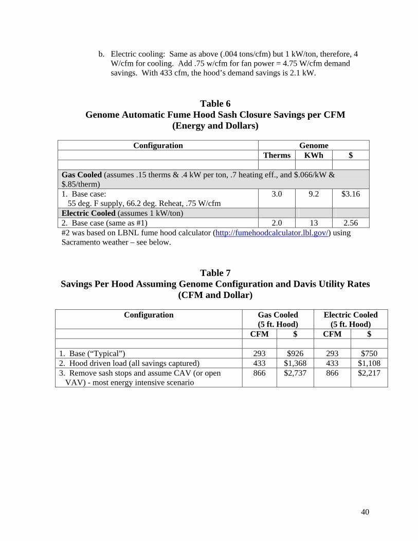
Table 6 Genome Automatic Fume Hood Sash Closure Savings per CFM


Configuration Genome Therms KWh $ Gas Cooled (assumes .15 therms & .4 kW per ton, .7 heating eff., and $.066/kW & $.85/therm) 1. Base case:

55 deg. F supply, 66.2 deg. Reheat, .75 W/cfm 3.0 9.2 $3.16

Electric Cooled (assumes 1 kW/ton) 2. Base case (same as #1) 2.0 13 2.56 #2 was based on LBNL fume hood calculator (http://fumehoodcalculator.lbl.gov/) using Sacramento weather – see below.

Table 7

Savings Per Hood Assuming Genome Configuration and Davis Utility Rates (CFM and Dollar)

Configuration Gas Cooled

(5 ft. Hood) Electric Cooled

(5 ft. Hood) CFM $ CFM $ 1. Base (“Typical”) 293 $926 293 $750 2. Hood driven load (all savings captured) 433 $1,368 433 $1,108 3. Remove sash stops and assume CAV (or open

VAV) - most energy intensive scenario 866 $2,737 866 $2,217

40

http://fumehoodcalculator.lbl.gov/

Genome- LBNL Fume Hood Calculator (http://fumehoodcalculator.lbl.gov/) Base Case with electric chiller and 293 cfm savings (limited by minimum lab air change):

41

Genome- LBNL Fume Hood Calculator (http://fumehoodcalculator.lbl.gov/) electric chiller and 433 cfm, savings (not limited by minimum lab air change):

42

B. Limitations Many factors affect the energy use and potential savings relating to laboratory fume hoods. The UC Davis case studies represented neither the best or worst opportunity. Characteristics that made them good opportunities included:

• VAV was already installed (lowers retrofit cost) • There was poor sash management (hoods left open)

Characteristics that reduced the potential savings included:

• Hood density was not high, such that general exhaust and cooling drive the required air flow (for example in the Genome building the 433 cfm potential hood savings was limited to approximately 293 cfm because of general exhaust needs

• Fume hood air flow was designed around a “restricted sash” - sash stops set at 18,” thus reducing the potential savings approximately 60% at PES and 50% at Genome (assuming a 36” max. opening at PES, a 30” max. opening at Genome, and a 24” counter depth inside the hood at both)

• A relatively small five foot hood was retrofitted at the Genome Building at the same cost, but with much less savings than a larger hood

• UC Davis enjoys abnormally low utility rates • Supply fan savings was linear and low (e.g. .32 and .75 watts per cfm vs. typical 1.8)

vs. a theoretical cubed function (static pressure reset could yield significantly more supply fan savings)

• No savings from the constant volume exhaust fans (savings could be increased with a reconfigured VAV or staged exhaust fan system)

43

C. Sensitivity Analysis

1. Steam driven cooling vs. electric driven chillers UC Davis uses steam absorption chillers as the prime driver for chilled water production. This has a major impact on the electric energy and demand savings associated with a more common electric chiller configuration. Therefore, savings was estimated for both scenarios:

Table 8 Automatic Fume Hood Sash Closure Savings per CFM

(Energy and Dollars) Configuration PES Genome

Therms KWh $ Therms KWh $ Gas Cooled (assumes .15 therms & .4 kW per ton, .7 heating eff., and $.066/kW & $.85/therm) 1. Base case:

PES: 63 deg. F supply, 74 deg. reheat, .32 W/cfm Genome: 55 deg. F supply, 66.2 deg. Reheat, .75 W/cfm

3.1 4.0 $2.90 3.0 9.2 $3.16

Electric Cooled (assumes 1 kW/ton) 3. Base case (same as #1) 2.6 5.8 $2.59 2.0 13 2.56

44

2. Fix PES Reheat The reheat system at the test lab in PES is stuck at a 74 deg. F supply temperature. If the reheat valve is fixed it is assumed that the supply temperature could be reduced to 70 deg. F. This will eliminate the need for additional general exhaust to cool the room and will reduce the amount of reheat (from 11 deg. to 7 deg. F).



Configuration PES Therms KWh $ Gas Cooled (assumes .15 therms & .4 kW per ton, .7 heating eff., and $.066/kW & $.85/therm) 2. Fix PES reheat 2.5 4.0 $2.39 Electric Cooled (assumes 1 kW/ton) 4. Fix PES reheat: reduce

to 70 deg F. 2.1 5.8 $2.17

3. Standard PES Supply Air Temperature (55 deg. F) The supply temperature at PES (from the AHU) is set at 63 deg. F; 55 deg. F is a more standard set point.



Configuration PES Therms KWh $ Electric Cooled (assumes 1 kW/ton) 5. Same as #4 w/ normal

55 deg. F supply, 70 deg reheat PES only)

1.9 9.2 $2.25

See PES results for a copy of the LBNL Fume Hood Calculator for this configuration.

45

4. UC Davis vs. PG&E utility rates Utility rates for UC Davis are lower than typical PG&E customers. The following estimates the savings per CFM using standard PG&E commercial rates for gas ($1.30/therm) and electricity ($.10/kWh):

Table 11 Automatic Fume Hood Sash Closure Savings per CFM, PG&E Rates


Configuration PES Genome Therms KWh $ Therms KWh $ Electric Cooled 6. Same as #5 w/

commercial PG&E rates (.10/kWh, 1.30/therm)

1.9 9.2 $3.44 2.0 13 3.90

This condition is considered the typical for commercial PG&E lab customers. PES - LBNL Fume Hood Calculator (http://fumehoodcalculator.lbl.gov/) 55 deg. F Supply, 70 deg. F Reheat and Commercial PG&E Utility Rates:

46

D. Economic Analysis

1. System Cost The automatic fume hood sash closure system is currently being marketed for $5,500 per hood installed in small quantities. The cost in larger quantities (e.g. a lab building with 80 hoods) was quoted at $4,300 per hood installed. In both cases there may be additional costs associated with providing electrical power and compressed air at the top of the hood, decontaminating the hood to allow working in and around it, and repairing the sash operation (if stuck or sticky). We believe as the market (volume) increases, and potential competitors enter the market, the price will reduce.

2. Energy Cost Savings

a) UC Davis A blended electric rate of $.066/KWh and an average gas rate of $.85/therm were used for analysis of the savings at UC Davis. As described under the sensitivity analysis, UC Davis has abnormally low rates. UC Davis also uses gas driven chillers which shift electric energy and demand charges from more commonly deployed electrically driven chillers. Both of these factors contribute to Davis being an unusual application. The annual savings for PES at UC Davis was $2.39 per cfm (assuming the reheat is fixed) and $3.16 per cfm at the Genome Building.

Table 12 Savings Per Hood Assuming Davis Configuration and Utility Rates

(CFM and Dollar)

Configuration PES (6 ft. Hood) Genome (5 ft. Hood)

CFM $ CFM $ 1. Base 533 $1,274 293 $926 2. Hood driven load (all savings captured) 533 $1,274 433 $1,368 3. Remove sash stops and assume CAV


1333 $3,186 866 $2,737

b) Typical PG&E Laboratory Customer To address the issue of UC Davis’s low utility rates and gas driven chillers, an analysis was done assuming standard PG&E commercial rates ($.10/kWh blended, and $1.30/Therm) and a typical electric driven chiller plant with an efficiency of 1 KW/ton (including distribution). In addition, PES had a leaking reheat valve wasting heat and increasing the cfm as the system tried to cool with 74 deg. F supply air. Further, the PES’s AHU supplies air at 63 deg. F vs. the more standard 55 deg. F. Sensitivity analysis described above, evaluated the impacts of these factors. A base case for a typical PG&E customer was developed assuming standard

47

commercial utility rates, standard 55 deg. F supply temperature, and a properly functioning reheat system. The annual savings for these typical conditions was $3.44 per cfm for an application similar to PES and $3.90 per cfm for conditions similar to Genome. Note these values are below “rules of thumb” that often assume $5/cfm. This is likely due to the mild climate, high fan efficiency (.32 and .75 W/cfm vs. 1.8 default in web calculator), and no savings from the exhaust fan (constant volume).

Table 13 Savings Per Hood Assuming Typical Configuration and PG&E Utility Rates

(CFM and Dollar)

Configuration PES (6 ft. Hood) Genome (5 ft. Hood)

CFM $ CFM $ 1. Base 533 $1834 293 $1,143 2. Hood driven load (all savings captured) 533 $1834 433 $1,689 3. Remove sash stops and assume CAV


1333 $4586 866 $3,377

48

Genome - LBNL Fume Hood Calculator (http://fumehoodcalculator.lbl.gov/) 55 deg. F Supply, 66.2 deg. F Reheat, 433 cfm savings and Commercial PG&E Utility Rates:

3. Other considerations – new construction If the automatic fume hood sash closure system is deployed in new construction, and the design team assumes a small fraction of the hoods are simultaneously open, the reduced infrastructure (fans, ducts, boilers, chillers, etc.) size and cost will offset the increased hood control cost.

E. Issues Encountered Most of the issues that were encountered related to specific site characteristics, for example, low utility costs, abnormal supply temperatures, and leaking valves. There were no systemic issues encountered relative to the emerging technology. However, a problem with misalignment of the sash safety sensor was noted. Fan savings lower than anticipated: The lack of significant fan savings at the margin (in the operating range) was a surprise. Fan laws that would put the reduction of power as the cube of the reduction of flow are often quoted relative to the potential savings associated with airflow controls. However, what is more important is the system curve and how the system

49

is controlled. Both demonstration projects had variable speed drives on the supply fans. They did respond to changes in the system, however, only to reduce the flow, not the pressure. Controlling fans to a fixed static pressure is a common strategy but the energy savings is not nearly as great. As airflow to an individual lab is reduced, the air control valve closes, increasing the pressure drop to that zone. There is significant potential savings to reset the static pressure of the system as the airflow requirement is reduced. In PES the average fan watts per cfm was higher than (over twice) the savings at the margin (operational range). Thus PES is operating low on the curve where the slope is relatively flat. As the airflow increases, the system curve (watts per cfm) gets steeper. This is the case at Genome where the average watts per cfm is lower than the savings at the margin. However, the average fan power as well as the fan savings in both buildings was lower than the average watts per cfm found in many laboratory designs. Sash safety sensor: An “electric eye” sensor along the leading edge of the sash stops the sash closure if anything is protruding from the fume hood. In this demonstration, the sensors in both hoods lost alignment and failed within several months of operation. In circumstances where a sash sensor misalignment occurs, the sash on the fume hood is fully functional manually, but the automatic closure does not operate. Such a condition could go undetected, rendering the system ineffective for extended periods of time. This problem was discussed with the manufacturer who recommended an adjustment to the sensor’s sensitivity. Adjustments were made and the systems were returned to full operation. The problem seems less significant in other applications, but monitoring and maintenance is warranted to assure ongoing savings.

F. Feasibility for wide-spread implementation The results of these two demonstration projects would suggest that the emerging technology of automatic fume hood sash closure systems is feasible for wide-spread implementation. A challenge for wide-spread implementation is understanding the individual baseline and potential savings under specific applications – how much of the load is fume hood driven (vs. minimum lab airflow and cooling needs), what are the characteristics of the mechanical systems, what is the energy savings at the margin (specific operating range), and what is the existing sash management performance. It is difficult to generalize – every hood will have a different savings potential.

G. Market size and potential Fume hoods contribute to approximately 2,495 GWh/year, 574 MW, and 18 Trillion BTUs/year in California. The end-state goal is to reduce airflow through fume hoods by 75%. Energy savings is not directly proportional to airflow savings:

1. Two thirds of the KWh and one third of the KW savings are from the fans. In a static system, fan energy reduces at approximately the cube of the flow. Therefore a 75% reduction in fume hood flow can result in more energy savings, especially in the main supply fans which provide air for other purposes than the hoods (the impact will be at

50

the margin where flow reductions may have the greatest impact). However, more sophisticated controls will be required to achieve this potential than were present in this demonstration project.

2. Fume hoods don’t always “drive” the required air change rate. In labs with few hoods, other factors such as the minimum air change rate and thermal loads can dictate the required airflow. In these situations, reductions of airflow through the fume hoods are “made-up” by increases in the general room exhaust. This was the case in Genome.

If we assume that 1 and 2 cancel each other out for electricity, the end state goal will result in a 75% electrical savings, and if we further assume that the savings for natural gas is discounted 20% (of 75%) to yield a 60% potential savings, the overall potential is:

Saved Electricity GWh/year: 1,871 Saved Peak Power MW: 431 Saved Natural Gas Trillions BTUs/year: 11

This goal will be accomplished through multiple technology options. For example, since its introduction in the 1980’s, VAV has grown to a large market share in new construction. Assuming 30% of the hoods installed in California have VAV and 50% of the potential end state savings is achieved, VAV has already captured 15% of the potential savings outlined above. Assuming approximately 1/3 of the State’s estimated fume hoods are in the PG&E territory, and assuming a 35% market share for this emerging technology and a 10% market penetration per year, the added savings per year is estimated as:

Saved Electricity GWh/year: 22 Saved Peak Power MW: 5 Saved Natural Gas Billions BTUs/year: 200

51

VIII. Conclusions

Table 14 Automatic Fume Hood Sash Closure Annual Savings per CFM


Configuration PES Genome Therms KWh $ Therms KWh $ Gas Cooled (assumes .15 therms & .4 kW per ton, .7 heating eff., and $.066/kW & $.85/therm)1. Base case:

PES: 63 deg. F supply, 74 deg. F reheat, .32 W/cfm Genome: 55 deg. F supply, 66.2 deg. F Reheat, .75 W/cfm

3.1 4.0 $2.90 3.0 9.2 $3.16

2. Fix PES reheat: reduce to 70 deg. F

2.5 4.0 $2.39

Electric Cooled (assumes 1 kW/ton) 3. Base case (same as #1) 2.6 5.8 $2.59 2.0 13 2.56 4. Fix PES reheat: reduce

to 70 deg. F 2.1 5.8 $2.17

5. Same as #4 w/ normal 55 deg. F supply, 70 deg reheat PES only)

1.9 9.2 $2.25

Typical Conditions 6. Same as #5 w/

commercial PG&E rates (.10/kWh, 1.30/therm)

1.9 9.2 $3.44 2.0 13 3.90

52

Table 15

Savings Per Hood Assuming Typical Configuration and Utility Rates (CFM and Dollar)

Configuration PES (6 ft. Hood) Genome (5 ft.

Hood) CFM $ CFM $ 1. Base (“Typical”) 533 $1834 293 $1143 2. Hood driven load (all savings captured) 533 $1834 433 $1689 3. Remove sash stops and assume CAV


1333 $4586 866 $3377

Base (typical conditions) is configuration #6 in Table 14

Table 16 Demand Savings

Per CFM Per Hood

(533 cfm PES and 433 cfm Genome)

PES gas cooled 1.6 W .9 kW PES electric chiller 3.5 W 1.9 kW Genome gas cooled 2.3 W 1 kW Genome electric cooled 4.8 W 2.1 kW The above tables summarize the analysis of the demonstration project and the extrapolation to more typical practice (both in terms of system configuration as well as utility rates). At a cost of $4,500 per hood, the simple payback is 1 to 4 years based on the two test conditions and PG&E commercial rates. 2.3 to 2.5 year payback would be typical for a hood driven load. Low utility rates and other unique conditions at UC Davis yielded a lower unit savings and a longer payback. With the exception of PES’s assumed ton hours of cooling, and heating degree hours (to 63 deg. F), the estimates are based on field test data collected by UC Davis and Cogent Energy, and LBNL’s web based fume hood calculator, as well as the hand calculations shown. The fan system at PES provides much less savings at the margin than Genome (.32 W/cfm vs. .75 W/cfm) and much less than assumed as default in the LBNL fume hood calculator (1.8 W/cfm). These values result (along with other factors) in a lower overall savings of $2.39/cfm at PES vs. $3.16 at Genome. Typical industry values are double that, partially due to the higher fan energy mentioned, as well as higher utility rates. While the savings per cfm is lower at PES, the tested hood in Genome is smaller (5’ vs. 6’) and the savings in Genome

53

is further constrained by a minimum room exhaust (exhaust is not hood driven), so the cfm savings in PES is much higher than in Genome (533 cfm vs. 293 cfm). The fan savings could be significantly increased with a static pressure reset strategy (a potential retro commissioning opportunity). The reheat in the PES lab is out of control. It looks like the valve is stuck or leaking, adding approximately 11 deg. F whether it is desired or not. This is particularly a problem with the abnormally high supply air temperature (63 deg. F vs. 55 in Genome). When the room temperature rises, a lot more 74 deg. air at is required to maintain comfort, and this detracts from the savings due to sash control. The savings for reducing the reheat from 74 deg. to 70 deg. is shown in configuration #2 (first table). In calculating the savings per hood, the potential loss of savings with increased air flow was ignored and we assumed the reheat would be fixed and that the 63 deg. F supply air could maintain comfort at the minimum flow rate. Monitoring and maintenance of the sash safety sensor is required: To assure ongoing savings, monitoring and alarms should be established to check that the sash is being closed by the system (continuous monitoring based commissioning). Shortly after the demonstration period, the sash safety sensor on both hoods lost alignment and rendered the systems ineffective (reverting to manual control). Such a condition could go undetected. To improve performance, the sash closure control system itself could be monitored (dry contact in the control box indicating “obstruction”), or the fume hood exhaust airflow could be monitored to confirm the exhaust does not exceed the minimum for more than a few hours at a time. Such a monitoring system would alarm maintenance if potential savings are not being achieved. Generic conditions: While the demonstration analysis focused on specific applications at UC Davis, it is desirable to reach more “generic” conclusions. Therefore, the impact of using electric chillers for both buildings was evaluated. Electric cooling is less expensive than the existing gas cooling based on the assumptions made (see first table configuration #3+). Other “normalization” measures included:

• PES was analyzed for a more common 55 deg. supply air temperature (already used by Genome, see configuration #5).

• UC Davis has abnormally low utility rates ($.066/kWh and $.85/therm) so more standard commercial rates ($.10/kWh and $1.30/therm) were used to estimate savings of $3.44 to $3.90/cfm for “off campus” labs (configuration #6).

Even with these adjustments, the mild climate, low marginal cost/savings of supply air, and no savings on the exhaust air, yields an estimated savings lower than the often quoted “rule-of-thumb” of $5+/cfm. The generic savings rates of $3.44 and $3.90/cfm were applied to the actual hood cfm savings in PES and Genome. As noted, the air change rate in the Genome lab was not hood driven and the savings was constrained to 293 cfm. Had a 5 ft hood been retrofitted in a hood driven lab (as in PES), the savings would have increased to approximately 433 cfm (second table, configuration #2). In both cases, we assumed air flow savings derived from a

54

12” reduction is sash height (while staying above the minimum flow assuming a 24” deep interior). UC Davis already had installed two fume hood efficiency measures:

1. VAV fume hood controls 2. Restricted sashes (sash stops)

The sash stops restrict the sashes from fully opening. This was particularly effective at the “tall” hood in PES. If the sash stops were not used and the hoods were left fully open (or CAV hoods were used), the savings would have been much higher (i.e. approximately 1333 cfm for PES, and 866 for Genome). These are extreme conditions and represent the maximum potential savings from the technology (see second table, configuration #3). As the table below shows, the increase in minimum airflow required for Genome significantly detracted from the savings due to the auto closure system: Approximate breakdown of airflow PES Genome Genome w/ min air

driven by room Airflow saved by sash stop: 50% 40% 40% Airflow saved by auto closure system: 33.3% 40% 28% Minimum airflow (not savable): 16.7% 20% 32% Bottom line: At $3.44 to $3.90 per saved cfm (many hoods are higher), a typical 5 or 6 foot hood would save approximately $1689 to $1834 per year with this emerging technology. If a static pressure reset strategy is integrated with the retrofit, the savings could be greater. Gas use dominated the savings (even with electric chillers). Low utility rates at UC Davis reduce the savings approximately one third. To estimate the savings in a building or set of buildings, an analysis of the number and size of hoods, as well as the size of the rooms is required. Savings would need to be adjusted (down) for VAV hoods demonstrating better sash management, as well as labs with significant heat gain.

IX. Recommendations for Future Work The following actions are recommended:

1. Develop baselines (e.g. average sash position). Need to develop baselines for various applications and confirm improvement (time intervals and degree of sash opening by time-of-day before and after installation). Degree of diversity and opportunity for savings is generally unknown, and may vary by type of hood application as well as “corporate culture.” Further the degree to which fume hoods drive the exhaust air volume (vs. the minimum general exhaust or thermal requirements) is not known.

55

Such an analysis would be required to establish market incentive programs. While two hoods were evaluated in this study, a much more robust sample size is required.

2. Run side-by-side tests. Independent evaluation of options is needed for the market to understand and compare competing hood efficiency technologies.

3. Perform Impact Analysis and Prepare Business Case. Although a potential for significant energy savings appears to exist, our statewide energy impact analysis is generalized and hinges on a number of key assumptions. Improved data are needed on the overall population of hoods, current sales rates, geographical distribution, and baseline energy use of standard hoods across a range of industry and climatic settings. Improved energy analysis, coupled with cost-benefit information, should be assembled into a coherent business case. The potential for retrofit-driven savings and new market segments (e.g. wet benches) should also be identified and analyzed.

4. Develop Industry Partnerships. Liaisons should be maintained with industry organizations (AIA, ASHRAE, Labs21), as well as major design influencers (key lab planners and specialized A&E firms) and major users of fume hoods (e.g. R&D labs, and universities).

5. Information Transfer. Information transfer should include technical guidelines (e.g. fume hood design/selection guide), education/training (e.g. advanced workshop on fume hoods), and direct technical assistance (providing customers with access to technical experts). Outreach activities should include development and maintenance of a Taming the Hood website, presentations, and publications in professional and popular literature. A slide presentation is included in the Appendix.

6. Develop incentive programs. The current retrofit cost is quite high and the savings is not well understood (see “need to develop baselines”). Utility rebates can be used to provide market incentives, offset costs, and add credibility, thus increasing market acceptance.

7. Product development. More analysis and perhaps some product development on the sash safety sensor may be warranted. This sensor determines if something is protruding from the hood to stop the sash from hitting it. The system fails in the manual mode, and in our demonstration, both hoods failed due to misalignment of the sensors within several months of operation. At least one competitor uses a pressure sensitive switch along the leading edge of the sash. While this system is less prone to misalignment, it could result in experimental apparatus being knocked and perhaps damaged prior to activating the switch.

X. Appendices See attached for the following:

A. Monitoring and Evaluation Plans B. PG&E Brochure C. Test Site Solicitation and Requirements D. Power Point Presentation E. Report to Campus

56

A. Monitoring and Evaluation Plans Preliminary LBNL Plan October 9, 2006 Cogent Plan June 11, 2007 – See Appendix E: Report to Campus

57

Automatic Fume Hood Closure System Pilot Test DRAFT Monitoring and Evaluation Plan October 9, 2006 Dale Sartor. (510) 486-5988

1. Assess existing sash management a. Minimum: Observe sash position and interview user(s) to estimate sash

position over 24 hour/7 day period (typical week) b. Ideal: Sash monitoring or exhaust airflow monitoring to determine typical

sash position over 24 hour/7 day period c. Develop sash position schedule for typical week

2. Estimate exhaust air flow at various sash positions (including closed) a. Minimum: Use design data b. Ideal: Use existing monitoring system c. Confirm with one-time face velocity measurements

3. Based on 1 & 2, develop schedule of: a. Typical exhaust airflow for test hood

4. Confirm supply airflow responds to changes in exhaust airflow a. Minimum: Note air velocity at register changes as fume hood sash is opened

and closed b. Ideal: Use existing supply airflow monitoring system

5. Develop schedule of supply airflow a. Minimum: Use observations, design data, and engineering assumptions b. Ideal: Use existing monitoring of airflow or fan motor speed c. Develop schedule of estimated supply fan airflow

6. Estimate supply fan energy at various air flows a. Minimum: Use design data and engineering assumptions b. Ideal: Use existing monitoring of KW or fan motor speed c. Check with one-time KW measurement d. Develop schedule of estimated supply fan energy at various flows

7. Based on 5 and 6 develop spread sheet model (schedule) of supply fan airflow and energy use

8. Monitor KW at supply fan for various sash positions of the test hood a. If the system is small (change in energy detectable for one hood) and stable

(little variation), differences in fan energy based on test hood sash position should be captured and used

9. Based on 3, 7, and 8 develop spread sheet model of supply air flow and fan energy as a function of fume hood exhaust

a. A function of the test hood exhaust (all other hoods constant) • This model will be used to calculate before and after supply fan energy

use and savings for the test hood b. A function of the all hoods

• This model is expected to be less robust than the first, but would be used to estimate savings if all existing fume hoods served by the supply fan were to be retrofitted with the automatic fume hood sash closure system

58

• This model should account for a minimum general exhaust of 1 cfm per square foot (assuming a completed retrofit would remove the fume hoods from being the exhaust system “driver”)

10. Assess energy impact of VAV on fume hood exhaust system a. Exhaust system impact will likely be less than supply and will depend on the

configuration of the system (could be negligible) b. If potential savings from exhaust fan is not negligible develop similar spread

sheet model as described in 9. 11. Assess cooling system cost as a function of airflow

a. Using design data, engineering judgment, and readily available measured data, estimate average cooling system efficiency (KW/Ton)

b. Using design data, engineering judgment, and readily available measured data, develop spread sheet model of estimated cooling energy as a function of airflow

c. Unless better data is available: • Assume .6 KW/ton overall system efficiency • Assume 55 deg F supply air • Use bin temperature data and assume 24 hour operation

12. Assess re-heat system energy cost as a function of airflow a. Using design data, engineering judgment, and readily available measured data,

estimate average heating system efficiency (%) b. Using design data, engineering judgment, and readily available measured data,

develop spread sheet model of estimated heating energy as a function of airflow

c. Unless better data is available: • Assume air handler supply air temperature reduced to 55 deg F at outdoor

conditions above 55 deg F • Assume re-heat (zone supply) temperature is 65 deg F • Assume 70% overall heating system efficiency • Use bin temperature data and assume 24 hour operation

13. Assess post retrofit sash management a. Minimum: Monitor sash closure system to determine minutes per week that

the sash is open. Observe sash position and interview user(s) to estimate open sash position

b. Ideal: Sash monitoring, exhaust airflow monitoring, or monitor on auto sash closure system will determine sash position over 24 hour/7 day period (typical week)

c. Develop sash position schedule for typical week 14. Using schedules and models developed for exhaust and supply airflow, and energy

consumption for fans, cooling plant and heating plant, estimate energy consumption and savings

a. Based on one hood retrofit (test condition) b. All hoods retrofitted

15. Visit the site to review system in operation. Interview available facility managers and users (operators) to determine acceptance, strengths and weaknesses of the automatic fume hood closure system.

59

B. PG&E Brochure

60

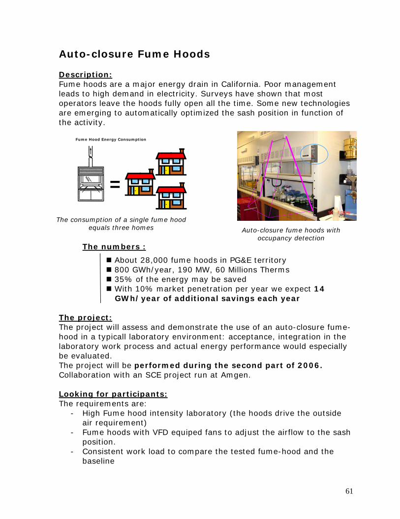
Auto-closure Fume Hoods Description: Fume hoods are a major energy drain in California. Poor management leads to high demand in electricity. Surveys have shown that most operators leave the hoods fully open all the time. Some new technologies are emerging to automatically optimized the sash position in function of the activity.

Fume Hood Energy Consumption

=

The consumption of a single fume hood equals three homes Auto-closure fume hoods with

occupancy detection The numbers :

About 28,000 fume hoods in PG&E territory 800 GWh/year, 190 MW, 60 Millions Therms 35% of the energy may be saved With 10% market penetration per year we expect 14 GWh/year of additional savings each year

The project: The project will assess and demonstrate the use of an auto-closure fume-hood in a typicall laboratory environment: acceptance, integration in the laboratory work process and actual energy performance would especially be evaluated. The project will be performed during the second part of 2006. Collaboration with an SCE project run at Amgen. Looking for participants: The requirements are:

- High Fume hood intensity laboratory (the hoods drive the outside air requirement)

- Fume hoods with VFD equiped fans to adjust the airflow to the sash position.

- Consistent work load to compare the tested fume-hood and the baseline

61

C. Test Site Solicitation and Requirements

62

PG&E and LBNL Looking for Fume Hood Auto Sash Closure Demo Site PG&E and LBNL have initiated a project to demonstrate an emerging fume hood technology. The technology automatically raises and lowers the fume hood sash depending on the user’s presence and preferences. A host site is being sought. The technology works in conjunction with an existing VAV fume hood control system to maximize energy efficiency and laboratory safety. The outside make-up air in the demonstration lab must be driven by the fume hood exhaust requirements. The demonstration will document the reduction in outside air and resulting energy savings. It will be done at a PG&E customer facility, and will require some cost sharing by the host site. If you are looking for ways to reduce the cost of operating fume hoods at your facility and would consider participating in this demonstration, please respond to this e-mail or contact Francois Rongere at PG&E (415-973 6856), or Dale Sartor at LBNL (510-486-5988). Thank you for your consideration. Opportunity to Work With PG&E and LBNL On Demo of Fume Hood Auto Sash Closure There is still an opportunity for a laboratory owner to participate in the demonstration and evaluation of an emerging fume hood technology. PG&E and LBNL have initiated a project to demonstrate an off-the-shelf technology that automatically raises and lowers the fume hood sash depending on the user’s presence and preferences. A host site is being sought. The technology works in conjunction with an existing VAV fume hood control system to maximize energy efficiency and laboratory safety. The outside make-up air in the demonstration lab must be driven by the fume hood exhaust requirements. The demonstration will document the reduction in outside air and resulting energy savings. It will be done at a PG&E customer facility, and will require some cost sharing by the host site. If you are looking for ways to reduce the cost of operating fume hoods at your facility and would consider participating in this demonstration, please respond to this e-mail or contact Alicia Breen at PG&E (415-973-0317), or Dale Sartor at LBNL (510-486-5988). Thank you for your consideration.

63

Automatic Fume Hood Closure System Pilot Test Site Requirements and Selection Criteria October 9, 2006 Dale Sartor, (510)486-5988 Requirements:

10. PG&E Customer 11. Customer willing to share performance information

a. Anonymity acceptable but not preferred 12. Customer willing to cost share

a. Purchase and install system (approximately $5K) b. In-house effort to support project

13. Existing VAV fume hood and room pressure control system 14. Hood driven load

a. Closure of hood results in reduced supply airflow to lab and reduced supply fan horse power

15. Poor existing sash management (based on visual inspection and interview(s)) 16. Low hazard lab with no obvious safety hazards or operational concerns (this does not

imply any type of formal evaluation) Desirable traits:

1. Easily monitored system, e.g. existing: a. Sash position or exhaust airflow monitor b. Supply airflow and temperature monitors

• Outside air • Supply air • Reheat

c. Supply fan energy (watts) or speed calibrated to watts 2. Easily accessible

a. Bay area location b. Limited security requirements

64

D. Power Point Presentation

65

66

67

68

69

70

71

72

73

74

75

76

E. Report to Campus

77

AUTOMATIC FUME HOOD CLOSURE PILOT

RESULTS SUMMARY

PLANT AND ENVIRONMENTAL SCIENCES LAB 1247 AND GENOME BUILDING LAB 1010,

UC DAVIS

Prepared for: UC DAVIS

Submitted on: 10/20/2007

Prepared by:

Cogent Energy, Inc. 2300 Clayton Road, Suite 480

Concord CA, 94520 Ph: (925) 521-9600

www.cogentenergy.com

Page 2 of 4

Background Two automatic fume hood sash closure devices were installed on a trial basis in two UC Davis laboratories. One each were installed in Genome Laboratory #1010 and Plant and Environmental Sciences (PES) Laboratory #1247, as part of an automatic fume hood closure pilot project. The primary objectives of the pilot project were as follows:

• Evaluating the feasibility of installing sash closure devices on fume hoods.

• Estimating the energy and demand impact of such a device, per the measurement & evaluation (M&E) plan dated June 11, 2007.

• Evaluating savings from auto closure device applied to both variable air volume and constant volume fume hoods.

Pacific Gas and Electric Company in conjunction with Lawrence Berkeley National Laboratory (LBNL) is compiling the results of this pilot project as applicable to institutional and non-institutional clients. The project background, technology being evaluated, Measurement and Evaluation (M&E) methodology, energy analysis, economic analysis and sensitivity analysis will be described in their report.

This report summarizes the energy and cost savings as applicable for UC Davis for the two test sites.

Appendix A and B include the profiles developed for analysis purposes as part of this project. The data behind these profiles was utilized in the energy models to accurately simulate the air handling systems with and without automatic fume hood sash closure devices installed.

Page 3 of 4

Savings Summary Table 1 and Table 2 provide a summary of the estimated energy and cost savings associated with the installation of a sash closure device for one fume hood each in PES #1247 and Genome #1010. The savings estimates were performed for two scenarios. The first (Table 1) assumes the use of steam absorption chillers as the prime mover for providing chilled water for the associated air handling units (AHU). The second (Table 2) assumes the use of centrifugal chillers as the prime mover.

The savings listed in these tables have been estimated based on customized energy models developed to simulate the HVAC energy use of the systems serving the test site at each building. These systems include:

Genome Building – AHU-4, Exhaust Fan EF-2 and forty four (44) associated terminal units

PES Building - AHU-4, Exhaust Fans EF-7 and EF-8 and thirty eight (38) associated terminal units

Table 3 and Table 4 illustrate the estimated savings and costs associated by extrapolating the results from Table 1 and Table 2 to all the associated fume hoods on the AHU serving the pilot laboratories.

A blended electric rate of $0.066/kWh and an average gas rate of $0.85/therm have been used for this analysis. Other assumptions relating to the energy use have been documented in the M&E Plan developed for this project and is included in Appendix A.

Data and input profiles from the measurement and evaluation process are included in Appendix B and Appendix C.

Page 4 of 4

Table 1. Estimated Energy and Cost Savings from one Auto Sash Closure Retrofit (using Steam Absorption Chillers at Chiller Plant) Steam Absorption Chiller

Baseline Post-Retrofit Savings

Fan kWh Cooling Aux. kWh

Cooling kWh

Cooling therms

Heating therms Fan kWh Cooling

Aux. kWhCooling

kWh Cooling therms Heating therms Fan kWh Cooling

Aux. kWhCooling

kWhCooling therms

Heating therms

PES 1246 329,941 55,725 0 20,897 84,978 328,826 55,255 0 20,721 83,939 1,115 470 0 176 1,039 1,137$ $6,594 5.80 Genome 1010 506,284 58,189 0 21,821 40,093 504,348 57,344 0 21,504 39,541 1,936 844 0 317 552 922$ $6,594 7.15

Cost Savings

Payback (yrs)

Davis

Utility Rate Schedule Location Cost

Table 2. Estimated Energy and Cost Savings from one Auto Sash Closure Retrofit (using Centrifugal Chillers at Chiller Plant)

Centrifugal ChillerBaseline Post-Retrofit Savings


Cooling kWh

Cooling therms


Aux. kWhCooling

kWh Cooling therms Heating therms Fan kWh Cooling

Aux. kWhCooling

kWhCooling therms

Heating therms

PES 1246 329,941 55,725 83,587 0 84,978 328,826 55,255 82,883 0 83,939 1,115 470 704 0 1,039 1,034$ $6,594 6.38 Genome 1010 506,284 58,189 87,283 0 40,093 504,348 57,344 86,016 0 39,541 1,936 844 1,267 0 552 737$ $6,594 8.95

Cost Savings

Utility Rate Schedule Location Cost Payback

(yrs)

Davis

Table 3. Estimated Economic Summary from retrofit of all associated fume hoods on the AHU serving the pilot laboratory (using Steam Absorption Chillers at Chiller Plant)

Baseline Savings


Cooling kWh

Cooling therms


Aux. kWhCooling

kWh Cooling therms Heating therms

PES 1246 329,941 55,725 0 20,897 84,978 42,362 17,846 0 6,692 39,478 $43,218 $174,800 4.04 Genome 1010 506,284 58,189 0 21,821 40,093 85,188 37,152 0 13,932 24,304 $40,575 $202,400 4.99

Cost Savings

Utility Rate Schedule Location

Steam Absorption Chiller

Cost Payback (yrs)

Davis

Table 4. Estimated Economic Summary from retrofit of all associated fume hoods on the AHU serving the pilot laboratory (using Centrifugal Chillers at Chiller Plant)

Baseline Savings


Cooling kWh

Cooling therms


Aux. kWhCooling

kWh Cooling therms Heating therms

PES 1246 329,941 55,725 83,587 0 84,978 42,362 17,846 26,769 0 39,478 $39,297 $174,800 4.45 Genome 1010 506,284 58,189 87,283 0 40,093 85,188 37,152 55,728 0 24,304 $32,411 $202,400 6.24

Davis

Utility Rate Schedule Location

Centrifugal Chiller

Cost Payback (yrs)

Cost Savings

APPENDIX A

MEASUREMENT AND EVALUATION (M&E) PLAN

AUTOMATIC FUME HOOD CLOSURE PILOT

MONITORING AND EVALUATION PLAN

PLANT AND ENVIRONMENTAL SCIENCES LAB 1247

AND GENOME BUILDING LAB 1010, UC DAVIS

PREPARED FOR: PACIFIC GAS & ELECTRIC COMPANY

AND LAWRENCE BERKELEY NATIONAL LABORATORY

Submitted on: 6/11/2007

Prepared by:

Cogent Energy, Inc. 2300 Clayton Road, Suite 480

Concord CA, 94520 Ph: (925) 521-9600

www.cogentenergy.com

Background As part of a pilot project to demonstrate and assess the effectiveness of automatic fume hood sash closure devices, Cogent Energy has developed this Monitoring & Evaluation Plan. The purpose of the Plan is to outline the methods that will be used to estimate the energy and demand savings realized from the trial installation of two of these devices in campus laboratories. The application of this device is intended for two position and Variable Air Volume (VAV) type laboratory airflow control systems.

The automatic fume hood closure device operates by closing the sash after a set interval (typically one minute, adjustable) if it does not detect an occupant or any activity in front of the fume hood. The device is intended to reduce fume hood exhaust airflow which should lead to a reduction of supply airflow.

It is expected that lower supply airflow will result in lower cooling and heating (including reheat) energy use. Energy and demand savings would be realized at the fans and in the central plant cooling and heating systems. Note that energy savings at the hot water and chilled water distribution pumps are assumed to be negligible and are not included in the savings boundary of this project.

The primary requirements for choosing the test sites were that they contain VAV type laboratory airflow control systems including Direct Digital Controls (DDC) on the supply and exhaust for airflow monitoring. After investigating a number of possible options such as Life Sciences Addition, CCM and Equine AC Lab (Maddy Lab) the project team selected PES #1247 and Genome Lab #1010 as pilot test sites.

PES Lab #1247 is an 11 foot by 32 foot laboratory with one 6 foot fume hood. Supply air is delivered to the room by air handler AHU-4 and regulated by a make-up air valve. Fume hood and general room exhaust is provided by a general exhaust air duct served by two constant-volume exhaust fans EF-7 and EF-8. There are 43 other make-up air valves on AHU-4 (total 44).

Genome Lab #1010 is a 21 foot by 39 foot laboratory with one 4 foot fume hood. Supply air is delivered to the room by air handler AHU-4 and regulated by a variable air volume terminal. Fume hood and general room exhaust is provided by a general exhaust air duct served by one constant-volume exhaust fan EF-2. There are 37 other VAV terminals on AHU-4.

Facility Contact Information Elaine Bose Safety Coordinator Department of Plant Sciences UC Davis Davis, CA 95616 (530) 752-6915 [email protected]

Debbie Decker Campus Chemical Safety Officer EH&S 167 Hoagland Hall, UC Davis Davis, CA 95616 (530) 754-7964 [email protected]

Project Objectives The primary objectives of the automatic fume hood closure pilot project are to:

• Evaluate the feasibility of installing sash closure devices on fume hoods.

• Estimate the energy and demand impact of using this device via this M&E process.

• Evaluate savings of VAV vs. constant volume hood control, and savings from auto closure vs. both existing VAV and constant volume operation.

The following sections present the methodologies that will be used to estimate the energy and demand impact of utilizing this device, specific to the two test sites.

Monitoring and Evaluation Approach The approach described here uses monitored data along with other observations, assumptions, calculations, and documentation to define baseline performance, and to estimate energy savings that are attributable to the project.

Sources of Expected Energy and Demand Reductions

It is expected that through the application of this technology, energy and demand reductions will be realized in the following systems:

1. PES

i. Supply fan energy and demand due to reduced airflow

ii. Cooling energy (via chilled water, measured in ton-hours) due to reduced ventilation rates (as this is a 100% outside air system)

iii. Heating energy (including reheat) due to reduced ventilation rates

2. Genome Building

i. Supply fan energy and demand due to reduced airflow

ii. Cooling energy (via chilled water, measured in ton-hours) due to reduced ventilation rates (as this is a 100% outside air system)

iii. Heating energy (including reheat) due to reduced ventilation rates

Note:

1. Exhaust Fans at both building are single speed constant volume type and minimal energy savings are expected.

2. Chilled Water pumping and cooling tower heat rejection energy savings at the central chiller plant and building level are included in the overall chiller plant kW/ton usage.

3. Hot water pumping energy savings at the building heating plants are not included.

Monitoring Equipment

The majority of the operational data for both test sites will be gathered using the existing Siemens Apogee Energy Management System (EMS). Please refer to the control points list in Appendix A.

Additionally, portable data loggers will be used to estimate the amount of heating (or reheat) by measuring the temperature difference across the reheat coil (combined with air flow from the EMS).

The fume hood face velocity will be spot checked during a field visit for both test sites.

The total fan supply airflow will be measured using the EMS for both test sites. The supply CFM for all the terminal units (or make-up valves) supplied by the test AHU will be added to arrive at the total supply airflow. Supply fan kW will also be made available through the EMS.

It is expected that a reasonable variation in AHU supply airflow and kW will be visible in the collected trend data and that data will be used to determine the change in power for a corresponding change in CFM in the operating range of the AHU i.e., a marginal ∆W/∆CFM parameter will be arrived at for both test sites.

Spot measurements of the exhaust fan kW will be conducted for both sites over the natural operating range (morning vs. late afternoon) to confirm the assumption that the exhaust fan kW is relatively constant for the single speed exhaust fan motors.

Temporary monitoring equipment will be installed at the test site at PES to determine the fume hood sash position in order to estimate the fume hood exhaust airflow using an average face velocity of 100 feet per minute.

Monitoring and Evaluation Procedure

The intent of this M&E procedure is to estimate the energy and demand impact of using this device and will be divided into the four following steps:

STEP 1 - Establish baseline operational profiles for fume hood sash position STEP 2 - Establish operational profiles with sash locked at full open STEP 3 - Establish post retrofit operational profiles for fume hood sash position STEP 4 – Establish supply/exhaust airflow profiles and estimate annual energy use for

STEPS 1, 2 and 3 and calculate energy savings

The process is aimed at developing baseline operational profiles (STEP 1) for the sash position. Corresponding profiles will be developed during STEP 2 (sash locked at the full open position) and STEP 3 (post retrofit). These profiles will then be extrapolated to annual profiles based on the measured data with the assumption that the sash usage during the monitored period is representative of typical use.

The corresponding AHU supply and exhaust airflow profiles will be developed during STEP 4 in the following manner.

AHU Supply Airflow profile

The AHU supply airflow needs to be determined for developing the AHU supply airflow profile. This control point was programmed in the EMS on May 25, 2007 after the automatic sash positioner installation on May 24, 2007. Thus AHU supply airflow data for the AHU is not available for the baseline or sash full open conditions.

The AHU supply airflow profile for a typical week for STEP 3 (post retrofit) will be developed using the trend data from May 25, 2007 onwards.

Lab supply airflow data for the baseline period (STEP 1) prior to the installation of the automatic sash positioner will be utilized to develop an hourly lab supply airflow profile. The difference in CFM between this profile and the hourly lab supply airflow for STEP 3, will be added to the AHU supply airflow profile from STEP 3 to establish a supply airflow profile for STEP 1.

Sustained trending over a week or two week period is not critical for STEP 2 as the fume hood will be full open and it is expected that the lab airflow will remain relatively constant. The fume hood will be locked open for a few minutes and the difference in lab supply airflow at such condition to the lab supply airflow from STEP 1, will be added to the AHU supply airflow profile from STEP 1 to establish a supply airflow profile for STEP 2.

Exhaust Fan Airflow profile

At PES, the exhaust fans EF-7 and EF-8 are dedicated to AHU-4 (which serves lab #1247) and the exhaust fan airflow profile for STEP 3 will be developed using the total exhaust airflow control point made available in the EMS on May 25, 2007.

At Genome, the exhaust fan EF-2 is not dedicated to AHU-4 (which serves lab #1010) and the exhaust airflow will be estimated either by (1) adding up the supply vs. exhaust offsets for each of the labs served by AHU-4 or (2) mathematically using the spot measurements of exhaust fan kW and engineering calculations.

It is assumed that there will be little or no change in the exhaust fan airflow and the exhaust fan airflow profile developed for STEP 3 will be utilized for STEP 1 and STEP 2.

Also in STEP 4, a customized energy model (spreadsheet based bin simulation) will be developed to estimate the annual energy use of the post retrofit condition based on the operational profiles developed in STEP 3 and STEP 4. The monitored points such as AHU supply air temperature and heating (including reheat) temperature will be utilized in the model to simulate the observed conditions as accurately as possible. Total fan airflow will be determined and utilized as described in the Monitoring Equipment section.

Also, the same model will be utilized to estimate the annual energy use corresponding to STEP 1 and STEP 2 by simply inserting the operational profiles developed for those “STEPs” and using the marginal ∆W/∆CFM parameter as applicable. The differences in annual energy use estimated by the models for the different “STEPs” will determine the energy and demand savings.

The following steps apply to both sites unless specifically noted.

STEP 1 - Establish baseline operational profiles

1. Assess baseline (restricted sash) sash management and develop sash position profile

a. Sash monitoring or fume hood exhaust airflow monitoring to determine typical sash position over a one or two week period

b. Develop sash position schedule for typical week

Note: Control points for sash position and fume hood airflow as well as general exhaust airflow are available at Genome building EMS. Temporary monitoring equipment to determine sash position and an assumed face velocity (at 100 fpm) will be used to establish the sash position and fume hood exhaust at PES.

2. Develop operational profiles for supply/exhaust airflow

a. These will be developed in STEP 4.

STEP 2 - Establish operational profiles with sash locked at full open

1. Assess sash management (Note: this is not applicable as the sash will be forced to remain

full open during this period).

2. Develop operational profiles for supply/exhaust airflow


STEP 3 - Establish post retrofit operational profile

1. Assess post retrofit sash management and develop sash position profile

a. Sash monitoring or fume hood exhaust airflow monitoring to determine typical sash position over a one to two week period

b. Develop post-retrofit sash position schedule for typical week

Note: Control points for sash position and fume hood airflow as well as general exhaust airflow are available at Genome building EMS. Temporary monitoring equipment to determine sash position and an assumed face velocity (at 100 fpm) will be used to establish the sash position and fume hood exhaust at PES.

2. Develop post-retrofit operational profiles for supply/exhaust airflow


STEP 4 – Calculate energy savings

1. Develop operational profiles for supply/exhaust airflow as explained in the Monitoring and Evaluation Procedure section.

2. Develop customized energy model to simulate energy use for STEPS 1, 2 and 3. The model will account for supply fan energy, exhaust fan energy, cooling energy and heating (including reheat) energy in the following manner.

a. Supply Fan Energy - Estimate supply fan energy using the supply airflow profile for the STEP 3 and the marginal ∆W/∆CFM parameter for STEP 1 and STEP 2.

Note: Fan kW and AHU CFM will be monitored directly using the EMS at both buildings. The marginal ∆W/∆CFM parameter developed during STEP 3 will be applied to the additional airflow in STEP 1 and STEP 2 to estimate additional fan KW.

b. Exhaust Fan Energy – Estimate exhaust fan energy using spot measurements of motor kW. Both buildings have single speed constant volume type exhaust fans and exhaust fan energy will remain relatively constant. Also, exhaust fan energy is not expected to change much between STEPS 1, 2 and 3.

Note: Where more than one exhaust fan is connected to a common plenum, exhaust fan energy will be calculated using design data and engineering calculations.

c. Cooling energy - Estimate cooling energy using the supply airflow profiles for the respective STEP, Outside Air Temperature (OAT) (for UC Davis Climate Zone) and Discharge Air Temperature (DAT) at the AHU. OAT and DAT will be monitored at the EMS. Although, it is intended to use the TMY 30 climatic data (OAT) for the UC Davis Climate Zone, the OAT is being monitored so that the operational profiles can be normalized based on weather if needed.

The cooling energy will be estimated by modeling electric centrifugal and absorption chillers as the source of chilled water. A chiller plant efficiency of 1 kW/ton will be used for electric centrifugal chillers. A COP of 0.8 will be used to convert CHW ton-hrs to estimate the equivalent gas usage at the absorption chillers at UC Davis chiller plant and an additional 0.4 kW/ton will be used to account for the auxiliary electric usage when using absorption chillers.

d. Heating energy (including reheat) - Estimate heating (and reheat) energy using the supply airflow profiles, Outside Air Temperature, Discharge Air Temperature (DAT) at the AHU and Reheat Air Temperature. Significantly less reheat energy is expected at PES as the building operates at a higher system DAT than Genome building. We will use a nominal heating plant efficiency of 70%.

2. Establish annual energy use for each STEP.

3. Determine energy savings between baseline energy use (STEP 1) and post-retrofit energy use (STEP 3) based on one hood retrofit.

4. Determine energy savings between baseline energy use (STEP 1) and post-retrofit energy use (STEP 3) based on retrofit of all hoods at the building.

5. Determine energy savings between sash locked at full open (STEP 2) and post-retrofit energy use (STEP 3) based on one hood retrofit. This step will help illustrate an example of savings for a site with poor sash management practices.

6. Determine energy savings between sash locked at full open (STEP 2) and post-retrofit energy use (STEP 3) based on retrofit of all hoods at the building. This step will help illustrate an example of savings for a site with poor sash management practices

7. Determine energy savings between constant volume operation and post-retrofit energy use (STEP 3) based on retrofit of all hoods at the building. (It is possible that operation under STEP 2 with sash locked open will be similar to a constant volume operation)

8. Determine the above energy savings for an alternate PES operating condition i.e., with a constant 55°F discharge air temperature.

Appendix A The following is a list of points to be trended by the EMS, to be used for the energy calculations

Table 1: Trending Points List at PES

Building PESLab # 1247Point Desciption Identifier Trend Interval Type Status Notes

1 Hood Sash position # 1247 5 mins AI Using temporary monitoring equipment2 Fume Hood Exhaust Airflow CFM # 1247 (HEV) Calculated from Sash position and assumed face velocity3 General Exhaust Airflow CFM # 1247 (EXV) 5 mins AI Calculate from Overall Exhaust Airflow & Hood Airflow4 Lab Supply Ariflow CFM # 1247 (MAV) 5 mins AI Exists5 Overall Exhaust Airflow CFM # 1247 5 mins AI Exists (EXV CFM + HEV CFM)6 Exhaust Fan Speed EF 7/8 NA NA NA * CAV Exhaust Fans7 Supply Fan Speed (Hz) AHU 4 5 mins AI Exists8 Supply Fan Static Pressure AHU 4 5 mins AI Exists9 Exhaust Fan Static Pressure EF 7/8 5 mins AI Exists

10 OAT -- 5 mins AI Exists11 DAT (at AHU 4) AHU 4 5 mins AI Exists12 Reheat Temp (at Diffuser) # 1247 5 mins AI Install Logger Using temporary monitoring equipment13 Reheat Valve Posn # 1247 5 mins AI Exists14 Room Temperature # 1247 5 mins AI Exists15 MAV Valve Position # 1247 (MAV) Not Available These will not be monitored16 HEV Valve Position # 1247 (HEV) Not Available These will not be monitored17 EXV Valve Position # 1247 (EXV) Not Available These will not be monitored18 AHU 4 Supply CFM AHU 4 5 mins AI Added19 EF7 & EF8 Exhaust CFM EF 7/8 5 mins AI Added

Table 2: Trending Points List at Genome

Building GenomeLab # 1010Point Desciption Identifier Trend Interval Type Status Notes

1 Hood Sash position # 1010 5 mins AI Exists2 Fume Hood Exhaust Airflow CFM # 1010 (HEV)3 General Exhaust Airflow CFM # 1010 (EXV)4 Lab Supply Ariflow CFM # 1010 (VAV) 5 mins AI Exists5 Overall Exhaust Airflow CFM # 1010 5 mins AI Exists (EXV CFM + HEV CFM)6 Exhaust Fan Speed EF 7/8 NA NA NA * CAV Exhaust Fans7 Supply Fan Speed (Hz) AHU 4 5 mins AI Exists8 Supply Fan Static Pressure AHU 4 5 mins AI Exists9 Exhaust Fan Static Pressure EF 7/8 5 mins AI Exists

10 OAT -- NA NA NA Use from PES11 DAT (at AHU 4) AHU 4 5 mins AI Exists12 Reheat Temp (at Diffuser) # 1010 5 mins AI Install Logger Using temporary monitoring equipment13 Reheat Valve Posn # 1010 5 mins AI Exists14 Room Temperature # 1010 5 mins AI Exists15 VAV Damper Position # 1010 (VAV Dmpr%) 5 mins AI To be programmed16 HOOD Damper Position # 1010 (Hood Dmpr%) 5 mins AI To be programmed17 EXH Damper Position # 1010 (Exh Dmpr%) 5 mins AI To be programmed18 AHU 4 Supply CFM AHU 4 5 mins AI Added

APPENDIX B

PLANT AND ENVIRONMENTAL SCIENCES (PES) PROFILES

PES

0

200

400

600

800

1,000

1,200

1,400

1,600

1,800

Mon, 03/1

9/07

Mon, 03/2

6/07

Mon, 04/0

2/07

Mon, 04/0

9/07

Mon, 04/1

6/07

Mon, 04/2

3/07

Mon, 04/3

0/07

Mon, 05/0

7/07

Mon, 05/1

4/07

Mon, 05/2

1/07

Mon, 05/2

8/07

Mon, 06/0

4/07

Mon, 06/1

1/07

Mon, 06/1

8/07

Mon, 06/2

5/07

Mon, 07/0

2/07

Labo

rato

ry C

FM

Supply CFM - Baseline Supply CFM - Post-RetrofitTotal EXH CFM - Baseline Total EXH CFM - Post-RetrofitFH CFM - Baseline FH CFM - Post-Retrofit

Figure 1.1: Laboratory Airflow - Raw Data - PES 1247

0

200

400

600

800

1,000

1,200

1,400

Mon, 03/1

9/07

Mon, 03/2

6/07

Mon, 04/0

2/07

Mon, 04/0

9/07

Mon, 04/1

6/07

Mon, 04/2

3/07

Mon, 04/3

0/07

Mon, 05/0

7/07

Mon, 05/1

4/07

Bas

elin

e C

FM

0

50

100

150

200

250

300

350

400

∆ L

ab C

FM

Supply CFM - Baseline Total EXH CFM - Baseline FH CFM - Baseline ∆ Lab CFM

Figure 1.2: Laboratory Baseline Airflow - Raw Data - PES 1247

0

200

400

600

800

1,000

1,200

1,400

1,600

1,800

Sun, 0

6/17/0

7

Sun, 0

6/24/0

7

Sun, 0

7/01/0

7

Sun, 0

7/08/0

7

Post

-Ret

rofit

CFM

(500)

(400)

(300)

(200)

(100)

0

100

200

300

∆ L

ab C

FM

Supply CFM - Post-Retrofit Total EXH CFM - Post-RetrofitFH CFM - Post-Retrofit ∆ Lab CFM

Figure 1.3: Laboratory Post-Retrofit Airflow - Raw Data - PES 1247

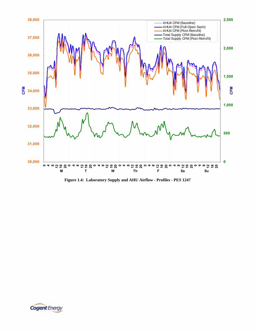
30,000

31,000

32,000

33,000

34,000

35,000

36,000

37,000

38,000

0 4 8 12 16 20 0 4 8 12 16 20 0 4 8 12 16 20 0 4 8 12 16 20 0 4 8 12 16 20 0 4 8 12 16 20 0 4 8 12 16 20

CFM

0

500

1,000

1,500

2,000

2,500

CFM

AHU4 CFM (Baseline)AHU4 CFM (Full-Open Sash)AHU4 CFM (Post-Retrof it)Total Supply CFM (Baseline)Total Supply CFM (Post-Retrof it)

M T W Th F Sa Su

Figure 1.4: Laboratory Supply and AHU Airflow - Profiles - PES 1247

0

5,000

10,000

15,000

20,000

25,000

30,000

35,000

40,000

Mon, 06/1

8/07

Mon, 06/2

5/07

Mon, 07/0

2/07

AH

U C

FM

AHU CFM - Post-Retrofit

Figure 1.5: AHU Post-Retrofit Airflow – Raw Data - PES 1247

0%

10%

20%

30%

40%

50%

60%

Mon, 05/0

7/07

Mon, 05/1

4/07

Mon, 05/2

1/07

Mon, 05/2

8/07

Mon, 06/0

4/07

Mon, 06/1

1/07

Mon, 06/1

8/07

Mon, 06/2

5/07

Mon, 07/0

2/07

Sash

Ope

n Po

sitio

n

Sash Position - BaselineSash Position - Post-Retrofit

21.1"

17.6"

14.1"

10.5"

7.0"

3.5"

0"

Figure 1.6: Sash Open Position - Raw Data - PES 1247

0%

10%

20%

30%

40%

50%

60%

0 4 8 12 16 20 0 4 8 12 16 20 0 4 8 12 16 20 0 4 8 12 16 20 0 4 8 12 16 20 0 4 8 12 16 20 0 4 8 12 16 20

Sash

Ope

n Po

sitio

n

Sash % Open (Baseline) Sash % Open (Post-Retrofit)

M T W Th F Sa Su

21.1"

17.6"

14.1"

10.5"

7.0"

3.5"

0"

Figure 1.7: Sash Open Position - Profiles - PES 1247

50

55

60

65

70

75

80

85

90

95

100

Mon, 03/1

2/07

Mon, 03/1

9/07

Mon, 03/2

6/07

Mon, 04/0

2/07

Mon, 04/0

9/07

Mon, 04/1

6/07

Mon, 04/2

3/07

Mon, 04/3

0/07

Mon, 05/0

7/07

Mon, 05/1

4/07

Mon, 05/2

1/07

Mon, 05/2

8/07

Mon, 06/0

4/07

Mon, 06/1

1/07

Mon, 06/1

8/07

Mon, 06/2

5/07

Mon, 07/0

2/07

Mon, 07/0

9/07

Mon, 07/1

6/07

Tem

pera

ture

, deg

. F

Post-Reheat DATAHU SAT

Figure 1.8: AHU Supply and Post-Reheat Discharge Temperatures – Raw Data - PES 1247

50

55

60

65

70

75

80

0 4 8 12 16 20 0 4 8 12 16 20 0 4 8 12 16 20 0 4 8 12 16 20 0 4 8 12 16 20 0 4 8 12 16 20 0 4 8 12 16 20

Tem

pera

ture

, deg

. F

Post-Reheat DAT

AHU SAT

M T W Th F Sa Su

Figure 1.9: AHU Supply and Post-Reheat Discharge Temperatures – Profiles - PES 1247

20,000

21,000

22,000

23,000

24,000

25,000

26,000

27,000

28,000

Mon, 06/1

8/07

Mon, 06/2

5/07

Mon, 07/0

2/07

AH

U4

SF W

atts

Figure 1.10: AHU Supply-Fan Power – Raw Data - PES 1247

20

21

22

23

24

25

26

27

28

0 4 8 12 16 20 0 4 8 12 16 20 0 4 8 12 16 20 0 4 8 12 16 20 0 4 8 12 16 20 0 4 8 12 16 20 0 4 8 12 16 20

AH

U S

F Po

wer

(kW

)

AHU kW (Post-Retrofit)

M T W Th F Sa Su

Figure 1.11: AHU Supply-Fan Power – Profile - PES 1247

y = 0.3154x + 14537.4555R2 = 0.4367

0

5,000

10,000

15,000

20,000

25,000

30,000

33,50

0

34,00

0

34,50

0

35,00

0

35,50

0

36,00

0

36,50

0

37,00

0

37,50

0

38,00

0

Post-Retrofit AHU4 CFM

AH

U4

SF W

atts

Based on AHU Watt and CFM hourly data

Airflow Cut-Off@ 34,000 CFM

Figure 1.12: AHU Power-Airflow (Watts-CFM) Correlation – Raw Data - PES 1247

APPENDIX C

GENOME PROFILES

0

200

400

600

800

1,000

1,200

1,400

Mon, 04/1

6/07

Mon, 04/2

3/07

Mon, 04/3

0/07

Mon, 05/0

7/07

Mon, 05/1

4/07

Mon, 05/2

1/07

Mon, 05/2

8/07

Mon, 06/0

4/07

Mon, 06/1

1/07

Mon, 06/1

8/07

Mon, 06/2

5/07

Mon, 07/0

2/07

Labo

rato

ry C

FMSupply CFM - Baseline Supply CFM - Post-RetrofitTotal EXH CFM - Baseline Total EXH CFM - Post-RetrofitFH CFM - Baseline FH CFM - Post-Retrofit

Figure 2.1: Laboratory Airflow - Raw Data – Genome 1010

0

200

400

600

800

1,000

1,200

1,400

Mon, 04/1

6/07

Mon, 04/2

3/07

Mon, 04/3

0/07

Mon, 05/0

7/07

Mon, 05/1

4/07

Bas

elin

e C

FM

(500)

(400)

(300)

(200)

(100)

0

100

200

∆ L

ab C

FM

Supply CFM - Baseline Total EXH CFM - Baseline FH CFM - Baseline ∆ Lab CFM

Figure 2.2: Laboratory Baseline Airflow - Raw Data - Genome 1010

0

200

400

600

800

1,000

1,200

Mon, 05

/21/07

Mon, 05

/28/07

Mon, 06

/04/07

Mon, 06

/11/07

Mon, 06

/18/07

Mon, 06

/25/07

Mon, 07/0

2/07

Post

-Ret

rofit

CFM

(500)

(400)

(300)

(200)

(100)

0

100

200

300

∆ L

ab C

FM

Supply CFM - Post-Retrofit Total EXH CFM - Post-RetrofitFH CFM - Post-Retrofit ∆ Lab CFM

Figure 2.3: Laboratory Post-Retrofit Airflow - Raw Data - Genome 1010

16,000

17,000

18,000

19,000

20,000

21,000

22,000

23,000

0 4 8 12 16 20 0 4 8 12 16 20 0 4 8 12 16 20 0 4 8 12 16 20 0 4 8 12 16 20 0 4 8 12 16 20 0 4 8 12 16 20

CFM

0

500

1,000

1,500

2,000

2,500

CFM

AHU4 CFM (Baseline) AHU4 CFM (Full-Open Sash)AHU4 CFM (Post-Retrofit) Total Supply CFM (Baseline)Total Supply CFM (Post-Retrofit)

M T W Th F Sa Su

Figure 2.4: Laboratory Supply and AHU Airflow - Profiles - Genome 1010

0

5,000

10,000

15,000

20,000

25,000

Mon, 06/0

4/07

Mon, 06/1

1/07

Mon, 06/1

8/07

Mon, 06/2

5/07

Mon, 07/0

2/07

AH

U C

FM

AHU CFM - Post-Retrofit

Figure 2.5: AHU Post-Retrofit Airflow – Raw Data - Genome 1010

0%

10%

20%

30%

40%

50%

60%

70%

Mon, 04/1

6/07

Mon, 04/2

3/07

Mon, 04/3

0/07

Mon, 05/0

7/07

Mon, 05/1

4/07

Mon, 05/2

1/07

Mon, 05/2

8/07

Mon, 06/0

4/07

Mon, 06/1

1/07

Mon, 06/1

8/07

Mon, 06/2

5/07

Mon, 07/0

2/07

Mon, 07/0

9/07

Sash

Ope

n Po

sitio

n

Sash Position - BaselineSash Position - Post-Retrofit

18.6"

13.3"

10.6"

8.0"

5.3"

2.7"

0"

15.9"

Figure 2.6: Sash Open Position - Raw Data - Genome 1010

0%

10%

20%

30%

40%

50%

60%

70%

0 4 8 12 16 20 0 4 8 12 16 20 0 4 8 12 16 20 0 4 8 12 16 20 0 4 8 12 16 20 0 4 8 12 16 20 0 4 8 12 16 20

Sash

% O

pen

Sash % Open (Baseline) Sash % Open (Post-Retrofit)

M T W Th F Sa Su

18.6"

13.3"

10.6"

8.0"

5.3"

2.7"

0"

15.9"

Figure 2.7: Sash Open Position - Profiles - Genome 1010

50

55

60

65

70

75

80

85

90

95

Mon, 03/2

6/07

Mon, 04/0

2/07

Mon, 04/0

9/07

Mon, 04/1

6/07

Mon, 04/2

3/07

Mon, 04/3

0/07

Mon, 05/0

7/07

Mon, 05/1

4/07

Mon, 05/2

1/07

Mon, 05/2

8/07

Mon, 06/0

4/07

Mon, 06/1

1/07

Mon, 06/1

8/07

Mon, 06/2

5/07

Mon, 07/0

2/07

Tem

pera

ture

, deg

. F

Post-Reheat DATAHU SAT

Figure 2.8: AHU Supply and Post-Reheat Discharge Temperatures – Raw Data - Genome 1010

45

50

55

60

65

70

75

0 4 8 12 16 20 0 4 8 12 16 20 0 4 8 12 16 20 0 4 8 12 16 20 0 4 8 12 16 20 0 4 8 12 16 20 0 4 8 12 16 20

Tem

pera

ture

, deg

. F

Post-Reheat DAT

AHU SAT

M T W Th F Sa Su Figure 2.9: AHU Supply and Post-Reheat Discharge Temperatures – Profiles - Genome 1010

0

2

4

6

8

10

12

14

Mon, 04/1

6/07

Mon, 04/2

3/07

Mon, 04/3

0/07

Mon, 05/0

7/07

Mon, 05/1

4/07

Mon, 05/2

1/07

Mon, 05/2

8/07

Mon, 06/0

4/07

Mon, 06/1

1/07

Mon, 06/1

8/07

Mon, 06/2

5/07

Mon, 07/0

2/07

AH

U S

F Po

wer

(kW

)

AHU4 kW - Baseline AHU4 kW - Post-Retrofit

Figure 2.10: AHU Supply-Fan Power – Raw Data - Genome 1010

0

2

4

6

8

10

12

14

0 4 8 12 16 20 0 4 8 12 16 20 0 4 8 12 16 20 0 4 8 12 16 20 0 4 8 12 16 20 0 4 8 12 16 20 0 4 8 12 16 20

AH

U S

F Po

wer

(kW

)

AHU kW (Baseline)

AHU kW (Post-Retrofit)

M T W Th F Sa Su Figure 2.11: AHU Supply-Fan Power – Profiles - Genome 1010

y = 0.7531x - 4516.9530R2 = 0.6687

0

2,000

4,000

6,000

8,000

10,000

12,000

14,000

19,00

0

19,50

0

20,00

0

20,50

0

21,00

0

21,50

0

22,00

0

AHU4 CFM

AH

U4

SF W

atts

Based on AHU Watt and CFM hourly data

Figure 2.12: AHU Power-Airflow (Watts-CFM) Correlation – Raw Data - Genome 1010

Documents

Automatic Fume Hood Sash Closure - Home | High … · 2017-09-20 · B. Genome Building Lab 1010 ... Debbie Decker, Campus Chemical Safety Officer, EH&S ... Automatic Fume Hood Sash