Embed Size (px)
Citation preview
symmetryS S
Article
Automatic Frequency Identification under SampleLoss in Sinusoidal Pulse Width Modulation SignalsUsing an Iterative Autocorrelation Algorithm
Alejandro Said 1,*, Yasser A. Davizón 2, Piero Espino-Román 3, Roberto Rodríguez-Said 4
and Carlos Hernández-Santos 5
1 Department of Computer Science, Tecnológico de Monterrey (Campus Monterrey),Eugenio Garza Sada 2501, Monterrey 64849, Mexico
2 Department of Mechatronics, Universidad Popular Autónoma del Estado de Puebla, 21 Sur 1103,Puebla 72410, Mexico; [email protected]
3 Department of Mechatronics, Universidad Politécnica de Sinaloa, Carretera Municipal Libre MazatlánHigueras Km 3, Mazatlán 82199, Mexico; [email protected]
4 Department of Mechatronics, Tecnológico de Monterrey (Campus Saltillo),Prolongación Juan de la Barrera 1241, Saltillo 25270, Mexico; [email protected]
5 Department of Mechatronics, Instituto Tecnológico de Nuevo León, Eloy Cavazos 2001, Guadalupe 67170,Mexico; [email protected]
* Correspondence: [email protected]; Tel.: +52-1-811-599-2728
Academic Editor: Ka Lok Man; Yo-Sub Han; Hai-Ning LiangReceived: 31 March 2016; Accepted: 29 July 2016; Published: 10 August 2016
Abstract: In this work, we present a simple algorithm to calculate automatically the Fourier spectrumof a Sinusoidal Pulse Width Modulation Signal (SPWM). Modulated voltage signals of this kind areused in industry by speed drives to vary the speed of alternating current motors while maintaininga smooth torque. Nevertheless, the SPWM technique produces undesired harmonics, which yieldstator heating and power losses. By monitoring these signals without human interaction, it is possibleto identify the harmonic content of SPWM signals in a fast and continuous manner. The algorithm isbased in the autocorrelation function, commonly used in radar and voice signal processing. Takingadvantage of the symmetry properties of the autocorrelation, the algorithm is capable of estimatinghalf of the period of the fundamental frequency; thus, allowing one to estimate the necessary numberof samples to produce an accurate Fourier spectrum. To deal with the loss of samples, i.e., the scanbacklog, the algorithm iteratively acquires and trims the discrete sequence of samples until therequired number of samples reaches a stable value. The simulation shows that the algorithm is notaffected by either the magnitude of the switching pulses or the acquisition noise.
Keywords: sinusoidal pulse width modulation; autocorrelation; power electronics; speed drives;signal processing
1. Introduction
In a normal Alternating Current (AC) power system, the voltage varies sinusoidally at a specificfrequency; usually 50 Hz or 60 Hz [1]. However, in some industrial applications, AC motors arerequired to work with different supply frequencies; thus, adjustable speed drives are used to solve thisproblem by varying the frequency of the input voltage.
In general, an oscilloscope is used to observe the voltage and current waveforms. An oscilloscopeis designed to capture a specific number of samples at a predefined sampling frequency; thus allowingthe operator to examine a plot of the samples on a screen. The operator needs, however, to knowthe fundamental frequency of the input signal in order to display an exact integer number of cycles.
Symmetry 2016, 8, 78; doi:10.3390/sym8080078 www.mdpi.com/journal/symmetry

Symmetry 2016, 8, 78 2 of 20
By knowing the fundamental frequency, the number of samples and sampling frequency can beadjusted exactly; otherwise, they need to be adjusted by trial and error. Nevertheless, if theseparameters are not adjusted correctly, the Fourier transform will not contain the actual spectrumof the original signal; resulting in discontinuities and spectral leakage; i.e., the spilling of energycentered at one frequency into the surrounding spectral regions [2,3]. Usually, to address this problem,the windowing technique is employed to reduce the amplitude of the discontinuities at the boundariesof each period, reducing spectral leakage [3]. This process, however, produces errors when estimatingthe amplitude of the spectrum harmonics, while the capacity for detecting weak frequency componentsnear strong components is also lost [2].
The waveform analyzed in the present study is the Sinusoidal Pulse Width Modulation(SPWM) [1,4–6], which is used widely in AC drives because it pushes the harmonics into ahigh-frequency range [4]; thus decreasing the mechanical vibrations that affect the performanceof AC motors. However, SPWM generates high-frequency harmonic components that lead to stresson the associated switching devices [1] and electrical power losses; such as rotor and stator windingheating, as well as eddy and hysteresis losses [7]. In order to implement preventive maintenance and adetailed diagnosis of AC machines and their drives, it is necessary to determine the magnitude andlocation of the harmonics in a fast and accurate manner.
In former studies, the zero-crossing method has been used as one of the simplest ways to estimatethe power system frequency; however, the measured signals typically contain harmonic distortions,which may introduce significant errors when using this method [8]. In some practical applications,the autocorrelation function [9–11] is used to identify the periodicities in an observed physical signal,which may be corrupted by a random interference [9]. In some recent studies, the problem of estimatingthe signal parameters for a sinusoidal waveform immersed in random noise has been addressed byusing the autocorrelation function [12–14]. There exists the non-parametric methods, which are basedon the idea of estimating the autocorrelation sequence of a random process from a set of measured dataand then taking the Fourier transform for estimating the power spectrum; and the parametric methods,which require some knowledge about how the data samples are generated [15,16]. In addition,the covariance matrices [17–19] can be used to estimate the power spectrum assuming that thevector samples are taken from a zero-mean multivariate random Gaussian process. Although thesemethods are suitable for voice, radar and communication applications, our method is a straightforwardengineering solution to a power electronics problem.
In the present study, we propose a frequency detection algorithm to deal with the problemof capturing a single SPWM signal cycle in a fast, automated and reliable manner. The pattern ofpulses [6] produced by SPWM gating signals is not random or small, but we use a simulation to showthat the autocorrelation function can be employed to identify the fundamental frequency of an SPWMsignal despite the magnitude of the pattern of pulses under conditions with scan backlog [20,21] andacquisition noise [22].
First, the original signal is autocorrelated to estimate its period, then the number of samplesrequired to process a single signal cycle is determined approximately. After those steps, the originalsignal sequence is trimmed iteratively until a single cycle can represent the Fourier spectrum accurately.A mathematical model is proposed for the scan backlog and used along with the acquisition noiseeffects in the steps of the algorithm.
The remainder of the article is organized as follows: In Section 2, we provide a summary ofthe background theory required to understand the proposed algorithm. Subsection 2.1 gives thedefinitions of the discrete Fourier transform, the root mean square (rms) and the Hanning window.An introduction to pure sinusoidal signal analysis is given to highlight the problem of capturing anon-integer number of cycles and to show why it is not convenient to use the windowing technique.Subsection 2.2 describes the relationship between time, the number of samples and the samplingfrequency. Subsection 2.3 presents the analysis of the autocorrelation and the period estimationof unknown frequency signals. Subsection 2.4 gives the background theory for SPWM signals:
Symmetry 2016, 8, 78 3 of 20
the definitions for the reference signal, the carrier signal, the number of pulses per half cycle and themodulation index. In Section 3, we explain each step of the flowchart for the proposed algorithm.In Section 4, we show the results for the estimation of the input signal frequency, including theeffects of the scan backlog and the signal noise. In Section 5, we give our conclusions regarding themain contributions of this study, as well as making suggestions for future research. In Appendix A,we include the parameter estimation of two signals, whose frequencies are non-integer. In Appendix B,the autocorrelation for periodic functions is defined.
2. Signal Analysis Background Theory
2.1. Analysis of the Spectrum Leakage at Sinusoidal Signals
In this subsection, we provide an analysis of the spectrum leakage of a sinusoidal signal in orderto highlight the need to acquire an integer number of cycles. In this analysis, we test a sinusoidal signalof 60 Hz and 200 volts-peak (Vp).
The discrete Fourier transform of a sequence of N samples is given by Equation (1), where xpnq isthe discretized signal and Xpkq are the spectrum harmonics [23].
Xpkq “N´1ÿ
n“0
xpnqe´j2πkn
N k “ 0, 1, 2, ..., N ´ 1 (1)
Equations (2) and (3) conform a modified version of the discrete Fourier transform,which is preferred in the present study. The factors 1{N and 2{N affect the height of each harmonicin order to represent its actual amplitude, where the coefficient 1{N is a normalizing factor used forthe reconstruction sum [24] and a multiplication by two is used in order to represent the one-sidedFourier spectrum [3]. The DC component, however, is not multiplied by two [3,7], as can be seenin Equation (2). The mathematical software tool used in this study is MATLAB [25]. It is importantto indicate that in order to ensure compatibility with this software, the lower and upper bounds ofthe summation are modified to start from n “ 1 and to end at n “ N. Furthermore, only half of theharmonics are used in the one-sided spectrum where k must be an integer; therefore, the index relatedto the location of each harmonic ranges from k “ 1 to the floor integer of half of the samples. Here, theMATLAB function fft(X) is used to calculate the discrete Fourier transform of a sequence. Later, theoutput of this MATLAB function is modified according to Equations (2) and (3).
Xpk´ 1q “1N
Nÿ
n“1
xpnqe´j2πkn
N k “ 1 (2)
Xpk´ 1q “2N
Nÿ
n“1
xpnqe´j2πkn
N k “ 2, 3, ..., tN{2u (3)
Equations (4)–(6) are used to calculate the rms value of the input signal, where Vrms is the totalrms value of the signal, VrmsDC is the rms value of the direct component and VrmsAC is the rms value ofthe alternate components of the signal. For example, Vrms1 denotes the rms value of the first harmonic,Vrms2 is the rms value of the second harmonic, and so on, up to Vrmsk [4], where the subscript krepresents the number of the spectrum harmonics used, as stated earlier.
VrmsDC “ VDC (4)
VrmsAC “
b
Vrms21 `Vrms2
2 ` ¨ ¨ ¨ `Vrms2k (5)

Symmetry 2016, 8, 78 4 of 20
Vrms “b
Vrms2AC `Vrms2
DC (6)
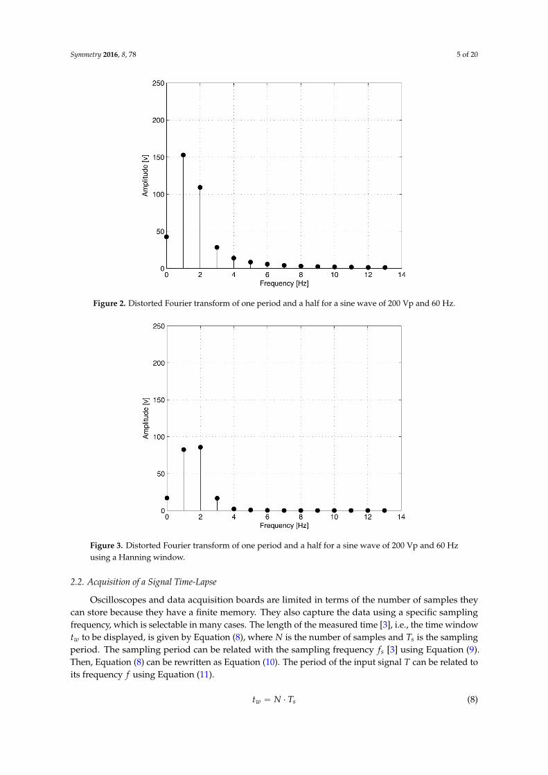
By displaying only 13 harmonics, the spectrum of an integer number of cycles for a sinusoidalsignal of 200 Vp and 60 Hz has a single impulse located at the first harmonic at 60 Hz with a magnitudeequal to the amplitude of the signal (as shown by the Fourier spectrum in Figure 1) and a rms valueof 141.4 V. Nevertheless, because the Fourier transform assumes periodicity, if one period and a half ofthe signal is acquired, then the result of the Fourier analysis would be the worst, as shown in Figure 2,where it can be seen that there is a nonexistent DCcomponent at 0 Hz with an amplitude of 42.4 V andseveral harmonics around the fundamental frequency with wrong amplitudes.
To reduce the magnitude of the nonexistent harmonics caused by acquiring a non-integer numberof cycles, a Hanning window [3] can be applied to the input signal. The Hanning window formula isgiven in Equation (7). A new windowed sequence of samples is obtained by multiplying each elementof the discretized signal xpnq by each element of the Hanning window hwpnq. In this case, the indexesof the Hanning window are assigned from n “ 1 to n “ N to ensure software compatibility.
hwpnq“0.5´0.5 cosp2πn{Nq; n“1, 2, 3, ..., N (7)
The resulting Fourier transform for one period and a half of the sine signal multiplied by theHanning window is shown in Figure 3, where the total rms value is 86.6 V; therefore, representing anerror of 38.7% calculated as | p141.4´86.6q| ¨ p100{141.4q.
Figure 1. Exact Fourier transform for a sine wave of 200 volts-peak (Vp) and 60 Hz.
The analysis above demonstrates in a simple, but reliable manner that the window technique isnot an appropriate solution when an accurate Fourier spectrum and its related calculations are needed,especially in power systems, where harmonics could be approximately hundreds of volts and shouldnot be neglected.
Symmetry 2016, 8, 78 5 of 20
Figure 2. Distorted Fourier transform of one period and a half for a sine wave of 200 Vp and 60 Hz.
Figure 3. Distorted Fourier transform of one period and a half for a sine wave of 200 Vp and 60 Hzusing a Hanning window.
2.2. Acquisition of a Signal Time-Lapse
Oscilloscopes and data acquisition boards are limited in terms of the number of samples theycan store because they have a finite memory. They also capture the data using a specific samplingfrequency, which is selectable in many cases. The length of the measured time [3], i.e., the time windowtw to be displayed, is given by Equation (8), where N is the number of samples and Ts is the samplingperiod. The sampling period can be related with the sampling frequency fs [3] using Equation (9).Then, Equation (8) can be rewritten as Equation (10). The period of the input signal T can be related toits frequency f using Equation (11).
tw “ N ¨ Ts (8)

Symmetry 2016, 8, 78 6 of 20
Ts “1fs
(9)
tw “Nfs
(10)
T “1f
(11)
For example, if a signal of 60 Hz is acquired, then the number of samples needed to displaya single cycle on the screen is N“ fsT“p100, 000qp1{60q “ 1666.6 samples at a sampling frequencyof 100 K samples per second, using tw “ T. Nevertheless, as shown in Formula (10), the time windowcan be adjusted by varying the number of samples, as well as the sampling frequency. The maximumsampling frequency, however, should be used in order to get the best resolution. For this simulation,we set the sampling frequency at a value of 100 K s/s, while the number of samples remains variable.
When setting a constant sampling frequency, a lower limit for the input signal frequency isrequired because more samples are needed to display a signal on the screen as the signal frequencyapproaches zero Hertz. For simulation purposes, the memory buffer is set to store a maximumof 20,000 samples, which is the number of samples needed to display a signal of 5 Hz at 100 K s/scorrectly; therefore, this simulation could not guarantee that the lower input frequencies would beanalyzed correctly.
2.3. The Autocorrelation Function
If xpnq is a discrete causal sequence, i.e., [xpnq “ 0 for n ă 0 and n ě N], then Equation (12)describes the autocorrelation sequence [9], where i “ l, k “ 0 for l ě 0 and i “ 0, k “ l for l ă 0.To save programming time, we used the MATLAB function xcorr(X) for calculating the autocorrelation,where X is a discrete sequence.
rxxplq “N´|k|´1
ÿ
n“i
xpnq ¨ xpn´ lq (12)
The autocorrelation function can be used to extract the fundamental frequency of a signalproducing a new sequence of samples of length 2N ´ 1. If a discrete time signal xpnq is periodic, thenits autocorrelation is also periodic with the same period [9,10]; i.e., its autocorrelation has large peaksevery period; however, because the sequence has a finite number of samples, the magnitude of peaksdecreases (see Appendix B for a detailed explanation about the autocorrelation of periodic discretesequences). Therefore, the period of the original signal can be obtained using the two autocorrelationindices that belong to the consecutive maximums or the minimums.
At first, rather than estimating one signal period, the amount of time corresponding to half of theperiod is computed using the lag indexes of the global maximum and global minimum, rmax and rmin,respectively. In general, this method is faster because most of the software packages have functionsto find the maximum and minimum values within a sequence (MATLAB functions rM, Is “ maxpAqand rM, Is “ minpAq were used). After numbering the autocorrelation lag indices from one to 2N ´ 1,the index of the global maximum value of the autocorrelation is lmax, and the index of the globalminimum value is lmin. Since the autocorrelation samples are separated by a distance Ts, half of theperiod can be estimated using T{2 “ Tsplmax ´ lminq; however, small acquisition errors may occur, sothe location of the global minimum cannot be determined accurately; i.e., the global minimum couldbe located to the right of the global maximum or to the left; therefore, an absolute value operation isneeded; i.e., T{2 “ Ts | plmax ´ lminq |; thus, the period estimation, can be obtained by doubling half ofthe signal period, as can be seen in Equation (13).

Symmetry 2016, 8, 78 7 of 20
Figure 4 illustrates the case where one and a half period of a sine wave of 200 Vp and 60 Hz hasbeen autocorrelated. For the example shown in Figure 4, the maximum and minimum indices arelmax “ 2500 and lmin “ 1667, respectively.
Figure 4. Autocorrelation of one cycle and a half for a sine wave of 200 Vp and 60 Hz.
T “ 2 Ts|plmax ´ lminq| (13)
For one period and a half of a sine wave of 200 Vp and 60 Hz, the calculation of the signalfrequency based on the determination of the period using the autocorrelation function yields 60.024 Hz;thus, there is a frequency estimation error of 0.04%.
2.4. The Sinusoidal Pulse Width Modulation
There are several SPWM techniques, such as bipolar SPWM [1] and unipolar SPWM [5,26,27].In the present study, we consider the unipolar SPWM technique. The gating signals for unipolarSPWM can be created by comparing a normalized sinusoid (the reference signal) and a triangularwaveform (the carrier signal) [4,5]. The amplitude of the reference signal is Ar, and the amplitude ofthe carrier signal is Ac. The modulation index M is the ratio of these signals (see Equation (14)), whichaffects the width of the pulses.
M “Ar
Ac(14)
The period of the reference signal Tr is the same as the period of the SPWM signal T;thus, the switching period of the carrier signal Tc [4] can be related to the number of pulses perhalf cycle p using Equation (15). It is important to note that the carrier period Tc depends on the SPWMperiod T; therefore, given the integer constant of 2pp` 1q, the carrier frequency is always constrainedto be a multiple of the SPWM frequency.
Tc “T
2pp` 1q(15)

Symmetry 2016, 8, 78 8 of 20
By rewriting Equation (15), the frequency of the carrier signal fc can be determined given thefrequency of the reference signal fr and the desired number of pulses per half cycle p, as can be seen inEquation (16). Equation (16) is a simpler form of Equation (15) because it involves the frequency of theSPWM signal. Here, the frequency of the reference signal is equal to the frequency of the SPWM signal;i.e., fr “ f .
fc “ 2 frpp` 1q (16)
This type of modulation eliminates all of the Low Order Harmonics (LOH) less than or equalto 2p´ 1, as shown in Equation (17). For example, when p “ 5, the LOH is the ninth [4].
LOH ě 2p´ 1 (17)
Figure 5 shows the resulting pattern of pulses for two periods of a reference signal of 60 Hz,with a modulation index of 0.5 and five pulses per half cycle. In this figure, the reference signal,the pattern of pulses and the carrier signal are displayed for the positive semi-cycle; but for clarity, onlythe reference signal and the pattern of pulses are shown for the negative semi-cycle. In this example,an unidirectional triangular wave is used as the carrier signal [4].
The voltage applied to the AC motor has the same shape as the pattern of pulses of Figure 5,but it is scaled to the available DC voltage of the speed driver. For example, if the available DC voltageat the speed driver is 200 V, then the amplitude of the SPWM is also 200 V; i.e., the peak voltageis 200 Vp.
Figure 5. Carrier signal, reference signal and pattern of pulses for an SPWM where p = 5 and M = 0.5.
Figure 6 shows a single period for the resulting SPWM signal produced by the pattern of pulsesin Figure 5, where the peak value is 200 V. Figure 7 shows the Fourier spectrum of the waveformillustrated in Figure 6 using the first 29 harmonics. The VrmsAC value of 111.6 V equals the total Vrmsvalue because there is no DC component. Figure 8 shows one period and a half of the same SPWMsignal, and Figure 9 shows the corresponding Fourier spectrum. Figure 9 shows, however, that there isa nonexistent DC component with an amplitude of 20.8 V and that Equation (17) is misled becausethere are several low order harmonics below the ninth harmonic.

Symmetry 2016, 8, 78 9 of 20
Figure 6. Single period for an SPWM signal of 200 Vp and 60 Hz, where p = 5 and M = 0.5.
Figure 7. Fourier spectrum of a single period for an SPWM signal of 200 Vp and 60 Hz.
Figure 8. One period and a half for an SPWM signal of 200 Vp and 60 Hz, where p = 5 and M = 0.5.

Symmetry 2016, 8, 78 10 of 20
Figure 9. Spectrum of one period and a half for an SPWM signal of 200 Vp and 60 Hz.
3. Automatic Fourier Spectrum Detection Using Autocorrelation
Figure 10 shows a flowchart of the proposed algorithm. Each step in the flowchart is indicated bya number enclosed in a gray circle and explained in the following list. Here, the boldface type is usedto indicate a sequence of values; the index n refers to a particular sample; the lowercase index i denotesthe latest calculated value; and the lowercase k is used to represent the location of each harmonic inthe Fourier spectrum. The maximum and minimum autocorrelation indices are not in boldface typebecause it is only necessary to retain their last calculations.
(1) In this step, a white noise signal wpnq is added to the original SPWM signal xpnq to simulate theeffect of the acquisition noise.
(2) Initially, because there is no information about the signal frequency, the algorithm retrieves theentire buffer to obtain a first approximation. In this step, the scan backlog is neglected becausethe sample loss is irrelevant.
(3) After being forced to enter the cycle for the first iteration, the algorithm compares the last twovalues regarding the number of samples needed to represent a single period. If these values differfor more than one sample, then the algorithm continues with the calculation; else, the Fourierspectrum is computed and displayed as indicated by Step 11.
(4) The signal autocorrelation is calculated. If this is the first iteration, the autocorrelation iscalculated for the 20 Ksamples; else, a trimmed version of the signal is used.
(5) The result of the autocorrelation is normalized in order to maintain a constant size in the verticalaxis of the screen.
(6) The lag indexes for maximum and minimum values in the autocorrelation are obtained.This is achieved by using the MATLAB functions rM, Is “ maxpXq and rM, Is “ minpXq,where X is a discrete sequence, M is the maximum or minimum value (according to the functionused) and I is the index where the value of interest is located.
(7) The signal period, the signal frequency and the number of samples necessary to represent asingle cycle are approximated by using Equations (10), (11) and (13), where the amount of timethat needs to be displayed is the period of the signal; i.e., tw “ T.
(8) In this step, a simulation of the scan backlog effect is considered. The scan backlog indicateshow much data remain in the buffer after each retrieval, providing a measure of how well theapplication is maintaining the throughput rate [20,23]; i.e., a Data Acquisition Card (DAQ) doesnot retrieve the data at the same rate as the sampling frequency fs. The retrieval speed refers tohow fast the computer is taking samples from the buffer toward a specific application.

Symmetry 2016, 8, 78 11 of 20
In this simulation, we assume a constant sampling frequency; hence, all of the samples areseparated by a time interval of Ts regardless of the retrieval speed.
Equation (18) shows our proposed model of the scan backlog. The scan backlog factor B istreated as a random variable that follows a uniform distribution; i.e., B~u(0,0.01). Therefore,the acquired number of N samples is reduced by 1% towards the actual number of samplesprocessed NB in the worst case. For example, a number of samples less than or equal to 200samples can be lost from a total of 20 K samples.
NB “ N ´ B ¨ N (18)
(9) In this step, the original digital sequence is trimmed according to the computed number ofsamples necessary to represent a single cycle; however, this parameter is affected by the scanbacklog effect; therefore, the algorithm needs at least two iterations to decide if the computednumber of samples is correct.
(10) In this step, a white-noise signal wpnq with a signal to noise ratio SNR “ 30 dB is added to theacquired SPWM signal xpnq to model the acquisition noise. In every iteration, a different whitenoise signal is used because the computer must simulate the start of a new acquisition.
Figure 10. Flowchart of the algorithm based on the autocorrelation function.

Symmetry 2016, 8, 78 12 of 20
4. Algorithm Evaluation Methodology
To test the effectiveness of the autocorrelation and the Equation (13) for estimating the periodSPWM signals, the autocorrelation is applied to the signal of Figure 8, which consists of one period anda half and a frequency of 60 Hz (see Figure 11). After applying Equations (13) and (11), the estimationof the signal frequency is 60.024 Hz; therefore, this estimation has an error of 0.04% regarding theactual frequency.
Figure 11. Autocorrelation function for one period and a half for an SPWM signal of 200 Vp and 60 Hz,with p = 5 and M = 0.5.
After verifying the effectiveness of the autocorrelation and Equation (13) by themselves, weproceed to prove the algorithm. Initially, the algorithm retrieves the entire buffer. Figure 12 shows theinitial screen, where 20 K of an SPWM signal of 200 Vp and 60 Hz were acquired.
Figure 12. Initial screen for an SPWM signal of 200 Vp and 60 Hz, where M = 0.5 and p = 5.
After running the algorithm illustrated in Figure 10, the final version of the input sequenceis presented in Figure 13, and its corresponding normalized autocorrelation is shown in Figure 14.In addition, the automated approximation of the Fourier spectrum produced by the algorithm ispresented in Figure 15, which resembles the exact Fourier spectrum of the SPWM signal shownin Figure 7.

Symmetry 2016, 8, 78 13 of 20
The final computation of the fundamental frequency of the SPWM signal, including the additionof the white noise and the effect of the scan backlog, is 60.024 Hz; therefore, there is an error of 0.04%regarding the actual input frequency of 60 Hz. After running the algorithm 30 times and including thewhite noise effect, the average calculation of the total rms value is 111.9 V, and the average estimationof the required number of samples is 1656.7 samples; representing an error of 0.2% in terms of the rmsvalue and an error of 0.5% in terms of the number of samples (with one decimal place of significance).The average number of iterations required by the algorithm to converge to a stable number of samplesunder these conditions is 5.9 iterations.
To compare the latest results, the white noise is removed. Then, the average rms value is 111.8 V,and the estimated number of samples is 1658.4 samples; therefore, representing an average rms errorof 0.2% and an error of 0.4% in terms of the required number of samples (with one decimal placeof significance). The average number of iterations required by the algorithm to converge to a stablenumber of samples under these conditions is 6.9 iterations.
Figure 13. Final trimmed version for an SPWM signal of 200 Vp and 60 Hz, where M = 0.5 and p = 5.
Figure 14. Final normalized autocorrelation function of the trimmed version for an SPWM input signalof 200 Vp and 60 Hz, where M = 0.5 and p = 5.

Symmetry 2016, 8, 78 14 of 20
Figure 15. Final Fourier spectrum of a trimmed version for an SPWM input signal of 60 Hz and 200 Vp.
5. Conclusions and Future Work
Regarding the present study, we can conclude that:
• It is important to represent a single SPWM signal period in the Fourier analysis; otherwise, theamplitude non-existing harmonics could lead to a poor electrical diagnosis. In industry, this couldaffect the preventive and corrective actions taken regarding the AC motors and their drives.
• The autocorrelation function can be applied to calculate the period of SPMW signals regardless ofthe magnitude of the pattern of pulses.
• The autocorrelation function can be used to estimate the period of SPWM signals under the lossof samples.
• The acquisition noise had no substantial effect in the calculation of the required numberof samples.
The main contributions of the present study are:
• Taking advantage of the symmetry of the autocorrelation, we have searched for the maximumand minimum value indexes regardless of the global maximum and minimum locations.This allowed for a rapid estimation of the signal period.
• We have provided a simple stochastic model for the scan backlog, to analyze the sample loss.• We have implemented an algorithm that uses the autocorrelation to iteratively calculate an
SPWM signal period despite the loss of samples and acquisition noise. Thus, we have provided asimulation under realistic conditions for an acquisition process.
As future work, the following opportunity areas remain:
• The scan backlog can also be modeled with variations in the sampling frequency arounda set point.
• In this study, the acquisition process commenced at the beginning of the positive semi-cycle;however, the variation of a specified trigger level can also be analyzed.
• The analysis of other PWM techniques using this algorithm is encouraged.• The proposed algorithm can be programmed into a real acquisition device to analyze SPWM
voltage and current signals.

Symmetry 2016, 8, 78 15 of 20
Finally, it is important to say that if this algorithm is implemented in modern oscilloscopes andpower analyzers, it could reduce the potential errors caused by the operator. The algorithm presentedin this work could also be used in control applications where an in-line calculation of the fundamentalfrequency (or other harmonic) is needed for a fast and continuous analysis of SPWM signals.
Acknowledgments: This study was supported by Consejo Nacional de Ciencia y Tecnología (CONACYT), locatedat Insurgentes 1582, Zip Code 03940, CDMX, México. Furthermore, this study was supported by Tecnológicode Monterrey (ITESM), located at Eugenio Garza Sada 2501, Zip Code 64849, Monterrey, Nuevo León, México.The costs for open access publishing where funded by Universidad Politécnica de Sinaloa, located at CarreteraMunicipal Libre Mazatlán Higueras Km 3, Zip Code 82199, Mazatlán, Sinaloa, México.
Author Contributions: Alejandro Said and Roberto Rodríguez-Said conceived the idea and performed thesimulations. Alejandro Said and Yasser A. Davizón wrote the paper. Piero Espino-Román and CarlosHernández-Santos analyzed and reviewed the data. Piero Espino-Román and Yasser A. Davizón, looked for thesuitable journal. All authors performed the literature review.
Conflicts of Interest: The authors declare no conflict of interest.
Appendix A
In this section, the algorithm is tested with non-integer frequencies, to prove that the algorithmworks correctly despite the round-off errors [23]. Two cases are provided: in the first case, the resultsare displayed for an SPWM signal of 33.7 Hz with p “ 5 and M “ 0.5; in the second case, the results aredisplayed for an SPWM signal of 99.3 Hz with p “ 9 and M “ 0.5. The acquisition noise is consideredfor both frequencies.
For the SPWM signal of 33.7 Hz, Figure A1 shows the screen where 20 K samples are initiallyacquired. Figure A2 shows the final trimmed version of the SPWM signal, and Figure A3 shows itscorresponding normalized autocorrelation used to calculate an approximated number of samples.Figure A4 shows the approximated Fourier spectrum obtained in an automated manner, where theLOH is the ninth. After running the algorithm 30 times, the average frequency calculation resultsin 33.715 Hz, representing an error of 0.012% regarding the exact frequency of 33.7 Hz. The averagecalculation of the total rms value is 111.9 V, representing an error of 0.3% regarding the exact rms valueof 111.5 V (with one decimal place of significance). The average estimated number of samples resultsin 2950.9 samples, representing an error of 0.5% regarding the exact number of 2967.3 samples (withone decimal place of significance). The average number of iterations required by the algorithm toconverge to a stable number of samples for this particular frequency is 16.8 iterations.
Figure A1. Initial screen for an SPWM signal of 200 Vp and 33.7 Hz, where p = 5 and M = 0.5.
For the SPWM signal of 99.3 Hz, Figure A5 shows the screen where 20 K samples are initiallyacquired. Figure A6 shows the final trimmed version of the SPWM signal, and Figure A7 shows its

Symmetry 2016, 8, 78 16 of 20
corresponding normalized autocorrelation. Figure A8 shows the approximated Fourier spectrum,where the LOH is the seventeenth. After running the algorithm 30 times, the average frequencycalculation results in 99.206 Hz, representing an error of 0.094 % regarding the exact frequencyof 99.3 Hz. The average calculation of the total rms value is 113.0 V, representing an error of 0.2%regarding the exact rms value of 112.7 V (with one decimal place of significance). The averageestimated number of samples results in 1003.2 samples, representing and error of 0.3% regardingthe exact number of 1007.0 samples (with one decimal place of significance). The average numberof iterations required by the algorithm to converge to a stable number of samples for this particularfrequency is 7.0 iterations.
Figure A2. Final trimmed version for an SPWM signal of 200 Vp and 33.7 Hz, with p = 5 and M = 0.5.
Figure A3. Final autocorrelation function of the trimmed version for an SPWM signal of 200 Vpand 33.7 Hz, with p = 5 and M = 0.5.

Symmetry 2016, 8, 78 17 of 20
Figure A4. Final Fourier spectrum of a trimmed version for an SPWM signal of 200 Vp and 33.7 Hz,with p = 5 and M = 0.5.
Figure A5. Initial screen for an SPWM signal of 200 Vp and 99.3 Hz, where p = 9 and M = 0.5.
Figure A6. Final trimmed version for an SPWM signal of 200 Vp and 99.3 Hz, with p = 9 and M = 0.5.

Symmetry 2016, 8, 78 18 of 20
Figure A7. Final autocorrelation function of the trimmed version for a SPWM signal of 200 Vpand 99.3 Hz, with p = 9 and M = 0.5.
Figure A8. Final Fourier spectrum of a trimmed version for an SPWM signal of 200 Vp and 99.3 Hz,with p = 9 and M = 0.5.
Appendix B
According to Proakis [9], the autocorrelation function of finite discrete sequences can be describedby Equation (12); however, if the discrete sequence is periodic with a period consisting of N samples,then the autocorrelation can be described by Equation (B1).
rxx “1N
N´1ÿ
n“0
xpnqxpn´ lq (B1)
Taking M samples of the signal in Equation (B2), where xpnq is a periodic sequence ofunknown period and wpnq represents a random interference, the autocorrelation can be described byEquation (B3).

Symmetry 2016, 8, 78 19 of 20
ypnq “ xpnq `wpnq (B2)
ryy “1M
M´1ÿ
n“0
ypnqypn´ lq (B3)
Substituting Equation (B2) in Equation (B3), Equation (B4) is obtained. Here, rxxplq is theautocorrelation of xpnq, the cross-correlation between the signal xpnq; the random interference wpnq isrepresented by rxwplq and rwxplq; and the term rwwplq is the autocorrelation of the random interference.Because xpnq is periodic, its autocorrelation has the same periodicity, presenting large peaks inl “ 0, N, 2N and every N multiple; however, when the displacement l tends to M, the peaksdecrease in amplitude, because there is a finite data storage consisting of M samples. In general,the cross-correlations rxwplq and rwxplq are small, because it is assumed that xpnq and wpnq are notrelated. Given the randomness of wpnq, its autocorrelation rwwplq tends rapidly to zero.
ryyplq “1M
M´1ÿ
n“0
rxpnq `wpnqsrxpn´ lq `wpn´ lqs
“ rxxplq ` rxwplq ` rwxplq ` rwwplq
(B4)
References
1. Reza, S.E. A Study on SPWM Boost Inverter and Its Reactive Power Control Strategy; Lap Lambert AcademicPublishing: Saarbrücken, Germany, 2012; pp. 12–19.
2. Rapuano, S.; Harris, F.J. An Introduction to FFT and Time Domain Windows. IEEE Trans. Instrum. Meas.2007, 10, 32–44.
3. Chugani, M.L.; Samant, A.R.; Cerna, M. LabView Signal Processing; Prentice Hall PTR: Upper Saddle River,NJ, USA, 1998; pp. 76–104.
4. Rashid, M.H. Power Electronics: Circuits, Devices and Applications; Pearson Prentice Hall: Upper Saddle River,NJ, USA, 2004; pp. 253–256.
5. Mohan, N.; Undeland, T.M.; Robbins, W.P. Power Electronics: Converters, Applications and Design; John Wileyand Sons, Inc.: Hoboken, NJ, USA, 2003; pp. 212–216.
6. Brown, M. Power Electronics in Motor Drives; Elektor International Media: London, UK, 2010; pp. 92–95.7. Llamas, A.; Acevedo, S.; Baez, J.A.; Reyes, J.A. Armónicas en Sistemas Eléctricos Industriales; Innovación
Editorial Lagares: Monterrey, México, 2004; pp. 56–59.8. Nam, S.; Kang, S.; Kang, S. Real-Time Estimation of Power System Frequency Using A Three-Level Discrete
Fourier Transform Method. Energies 2014, 8, 79–93.9. Proakis, J.G.; Manolakis, D.G. Digital Signal Processing; Pearson Prentice Hall: Madrid, Spain, 2007;
pp. 109–457.10. Rabiner, L.R. On the Use of Autocorrelation Analysis for Pitch Detection. IEEE Trans. Acoust. Speech
Signal Process. 1977, 25, 24–33.11. Shahnaz, C.; Zhu, W.; Ahmad, M.O. Pitch Estimation Based on a Harmonic Sinusoidal Autocorrelation
Model and a Time-Domain Matching Scheme. IEEE Trans. Audio Speech Lang. Process. 2012, 20, 310–323.12. Xiao, Y.; Wei, P.; Tai, H. Autocorrelation-Based algorithm for single-frequency estimation. Signal Process.
2007, 87, 1224–1233.13. Elasmi-Ksibi, R.; Besbes, H.; López-Valcarce, R.; Cherif, S. Frequency estimation of real-valued single-tone in
colored noise using multiple autocorrelation lags. Signal Process. 2010, 90, 2303–2307.14. Cao, Y.; Wei, G.; Chen, F.A. A closed-form expanded autocorrelation method for frequency estimation of a
sinusoid. Signal Process. 2012, 92, 885–892.

Symmetry 2016, 8, 78 20 of 20
15. Stoica, P.; Randolph, L.M. Spectral Analysis of Signals; Pearson Prentice Hall: Upper Saddle River, NJ,USA, 2005.
16. Hayes, M.H. Statistical Digital Signal Processing and Modeling; John Wiley and Sons: New York, NY, USA, 2009.17. Parker, B.J.; Luenberger, D.G.; Wenger, D.L. Estimation of structured covariance matrices. Proc. IEEE 1982,
70, 963–974.18. Zorzi, M.; Ferrante, A. On the estimation of structured covariance matrices. Automatica 2012, 48, 2145–2151.19. Cai, T.T.; Ren, Z.; Zhou, H.H. Estimating structured high-dimensional covariance and precision matrices:
Optimal rates and adaptive estimation. Electr. J. Stat. 2016, 10, 1–59.20. Eltahir, W.E.; Lai, W.K.; Ismail, A.F.; Salami, M.J. Hardware Design, Development and Evaluation of a
Pressure-based Typing Biometrics Authentication System. In Proceedings of the Eighth Australian and NewZealand Intelligent Information Systems Conference (ANZIIS), Sidney, Australia, 10–12 December 2003;pp. 49–54.
21. Wei, C.; Zhuang, Z. A CAN Network for Temperature Monitoring of Car Engine and Train Bogie.In Proceedings of the International Conference on Internet Computing and Information Services, (ICICIS),Hong Kong, China, 17–18 September 2011; pp. 302–305.
22. Skibinski, G.L.; Kerkman R.J.; Schlegel, D. EMI emissions of modern PWM AC drives. IEEE Trans. Ind. Appl.1999, 5, 47–81.
23. Rabiner, L.; Cooley, J.; Helms, H.; Jackson, L.; Kaiser, J. Terminology in digital signal processing. IEEE Trans.Audio Electroacoust. 1972, 20, 322–337.
24. Prandoni, P.; Vetterli, M. Signal Processing for Communications; CRC Press: Boca Raton, FL, USA, 2008;pp. 63–65.
25. Matlab. The MathWorks, Inc. Available online: http://www.mathworks.com/ (accessed on 16 July 2016).26. Yue, X.; Ma, X.; Wang, H. A conceit of unipolar N-multiple frequency SPWM and the main circuit topology.
In Proceedings of the IEEE 6th International Power Electronics and Motion Control Conference, Wuhan,China, 17–20 May 2009; pp. 1531–1534.
27. Patel, M.A.; Patel, A.R.; Vyas, D.R.; Patel, K.M. Use of PWM techniques for power quality improvement.J. Recent Trends Eng. Technol. 2009, 1, 99–102.
© 2016 by the authors; licensee MDPI, Basel, Switzerland. This article is an open accessarticle distributed under the terms and conditions of the Creative Commons Attribution(CC-BY) license (http://creativecommons.org/licenses/by/4.0/).