Automatic extraction of ground control regions and orthorectification of remote sensing imagery

Automatic extraction of ground control regions and orthorectification of remote sensing imagery

Cheng-Chien Liu 1,*

and Po-Li Chen 2

1Department of Earth Sciences, Earth Dynamic System Research Center, National Cheng Kung University, Tainan 701 Taiwan ROC

2Institute of Satellite Informatics and Earth Environment, National Cheng Kung University, Tainan 701 Taiwan ROC *Corresponding author: [email protected]

Abstract: We develop a fast and accurate method that is able to automatically select and match a large amount of ground control regions (GCRs) for orthorectifying remote sensing imagery. This new method is comprised of four modules, namely automatic extraction of GCRs, fast image-to-image matching, iterating and filtering of GCRs, and rigorous orthorectification. We assess the accuracy of this new method by processing the high-temporal- and high-spatial-resolution Formosat-2 imagery. Results show that the accurate orthoimage with a root mean square error of less than 1.5 pixels can be automatically generated from one standard Formosat-2

image (covering 12km × 12 km) in 55 minutes. This new method has been incorporated into the Formosat-2 automatic image processing system and has been used to produce orthoimages on a daily-basis.

2009 Optical Society of America

OCIS codes: (100.0100) Image processing; (100.2000) Digital image processing; (100.5010) Pattern recognition; (280.0280) Remote sensing and sensors; (280.4788) Optical sensing and sensors

References and links

1. A. M. Melesse, Q. Weng, P. S.Thenkabail, and G. B. Senay, "Remote sensing sensors and applications in environmental resources mapping and modelling," Sensors 7, 3209-3241 (2007).

2. A. da Silva Curiel, L. Boland, J. Cooksley, M. Bekhti, P. S. Stephens, Wei, and M. N. Sweeting, "First results from the disaster monitoring constellation (DMC)," Acta Astronautica 56, 261-271 (2005).

3. G. Tyc, J. Tulip, D. Schulten, M. Krischke, and M. Oxfort, "The RapidEye mission design," Acta Astronautica 56, 213-219 (2005).

4. C.-C. Liu, "Processing of FORMOSAT-2 daily revisit imagery for site surveillance," IEEE Trans. Geosci. Remote Sens. 44, 3206-3214 (2006).

5. C.-C. Liu, Y.-C. Chang, S. Huang, F. Wu, A.-M. Wu, S. Kato, and Y. Yamaguchi, "First space-borne high-spatial-resolution optical imagery of the Antarctic from Formosat-2," Antarctic Science 20, 605-606 (2008).

6. C.-C. Liu, Y.-C. Chang, S. Huang, S.-Y. Yen, F. Wu, A.-M. Wu, S. Kato, and Y. Yamaguchi, "Monitoring the dynamics of ice shelf margins in Polar Regions with high-spatial- and high-temporal-resolution space-borne optical imagery," Cold Regions Science and Technology 55, 14-22 (2009).

7. T. Scambos, H. A. Fricker, C.-C. Liu, J. Bohlander, J. Fastook, A. Sargent, R. Massom, and A.-M. Wu, "Ice Shelf Disintegration by Plate Bending and Hydro-fracture: Satellite Observations and Model Results of the 2008 Wilkins Ice Shelf Break-ups," Earth and Planetary Science Letters, (accepted) (2008).

8. C.-C. Liu, J.-G. Liu, C.-W. Lin, A.-M. Wu, S.-H. Liu, and C.-L. Shieh, "Image processing of FORMOSAT-2 data for monitoring South Asia tsunami," Int. J. Remote Sens. 28, 3093-3111 (2007).

9. C.-C. Liu, C.-L. Shieh, C.-A. Wu, and M.-L. Shieh, "Change detection of gravel mining on riverbeds from the multi-temporal and high-spatial-resolution Formosat-2 imagery," River Research and Applications, (in press) (2008).

10. M. Gianinetto, and M. Scaioni, "Automated Geometric Correction of High Resolution Pushbroom Satellite Data," Photogrammetric Engineering and Remote Sensing 74, 107-115 (2008).

11. T. Toutin, "Geometric processing of remote sensing images: models, algorithms and methods," Int. J. Remote Sens. 25, 1893-1924 (2004).

12. L. C. Chen, T. A. Teo, and J. L. Liu, "The Geometrical Comparisons of RSM and RFM for FORMOSAT-2 Satellite Images," Photogrammetric Engineering and Remote Sensing 72, 573-579 (2006).

13. H. I. El-Gamily, "Utilization of multi-dates LANDSAT_TM data to detect and quantify the environmental damages in the southeastern region of Kuwait from 1990 to 1991.," Int. J. Remote Sens. 28, 1773-1788 (2007).

#106147 - $15.00 USD Received 27 Jan 2009; revised 13 Mar 2009; accepted 27 Apr 2009; published 29 Apr 2009

(C) 2009 OSA 11 May 2009 / Vol. 17, No. 10 / OPTICS EXPRESS 7970

mailto:[email protected]

14. H. Hamandawana, F. Eckardt, and S. Ringrose, "Proposed methodology for georeferencing and mosaicking Corona photographs," Int. J. Remote Sens. 28, 5-22 (2007).

15. A. Altmaier, and C. Kany, "Digital surface model generation from CORONA satellite images," ISPRS Journal of Photogrammetry and Remote Sensing 56, 221-235 (2002).

16. S. Baillarin, J. P. Gleyzes, C. Latry, A. Bouillon, E. Breton, L. Cunin, C. Vesco, and J. M. Delvit, "Validation of an automatic image orthorectification processing," in Geoscience and Remote Sensing Symposium, 2004. IGARSS '04. Proceedings. 2004 IEEE International (IEEE, 2004), pp. 1398-1401.

17. A. Habib, K. Kim, S.-W. Shin, C. Kim, K.-I. Bang, E.-M. Kim, and D.-C. Lee, "Comprehensive Analysis of Sensor Modeling Alternatives for High-Resolution Imaging Satellites," Photogrammetric Engineering and Remote Sensing 73, 1241-1251 (2007).

18. C.-C. Liu, R. Huang, C.-L. Shieh, and J.-C. Lin, "Applications of FORMOSAT-2 imagery on monitoring the spatial and temporal variations of landslide: the case of the catchment area of Tseng-Wen reservoir," in preparation (2008).

19. R.-J. You, and H.-W. Hwang, "Coordinate Transformation between Two Geodetic Datums of Taiwan by Least-Squares Collocation," Journal of Surveying Engineering 132, 64-70 (2006).

20. C. Liu, S.-C. Wu, F.-T. Hwang, A.-M. Wu, and H. Chen, "Radiometric and geometric calibration of ROCSAT-2 image," in The 25th Asian conference on remote sensing(Chiang Mai, Thailand, 2004), pp. 465-470.

21. T. M. Lillesand, R. W. Kiefer, and J. W. Chipman, Remote sensing and image interpretation (John Wiley & Sons, 2004).

22. W. Förstner, "A Feature Based Correspondence Algorithm For Image Matching," International Archives of the Photogrammetry, Remote Sensing 26, 150-166 (1986).

23. A. Getis, and J. K. Ord, "The Analysis of Spatial Association by Use of Distance Statistics," Geographical Analysis 24, 189-206 (1992).

24. A. Getis, and J. K. Ord, "Local Spatial Statistics: An Overview," in Spatial Analysis: Modelling In a GIS Environment, P. Longley, and M. Batty, eds. (Geoinformation International, Cambridge, UK, 1996), pp. 261-277.

25. J. K. Ord, and A. Getis, "Local spatial autocorrelation statistics: Distributional issues and an application," Geographical Analysis 27, 286-306 (1995).

26. J. P. Lewis, "Fast Template Matching," Vision Interface, 120-123 (1995). 27. J. G. Liu, and J. Ma, "Imageodsey on MPI & GRID for co-seismic shift study using satellite optical

imagery," in Prob. of the UK e-Science All Hands Meeting 2004 (Nottingham, UK, 2004), pp. 232-239. 28. D. Rocchini, and A. Di Rita, "Relief effects on aerial photos geometric correction," Applied Geography 25,

159-168 (2005).

1. Introduction

Spaceborne remote sensing imagery is advancing fast both in spatial and temporal resolutions. For example, the commercially operated satellite WorldView-1 is now able to provide high-spatial-resolution imagery with 50 cm resolution [1]; meanwhile, deploying a group of satellites in constellation, such as the Disaster Monitoring Constellation [2] and the RapidEye Satellite Constellation [3], has effectively shortened the revisit time to less than one day. In the case of Formosat-2, the first satellite with a high-spatial-resolution (2m) sensor placed in a daily revisit orbit, both the spatial and temporal resolutions are enhanced in its coverage area [4]. Since more details of land cover and land use can be revealed at a much higher frequency, Formosat-2 imagery has ever-increasing applications in environmental monitoring [5-7], hazard assessment [8], orthomap generation, and land use management [9]. Ever since its successful launch on 20 May 2004, Formosat-2 has been providing multispectral images of the Taiwan area with 2m resolution for more than 2,500 km

2 every day. These images need to

be processed and orthorectified in a few hours to meet the requirements of various applications. However, the current bottleneck of orthorectification is the time-consuming and error-prone process of manual selection and matching of the ground control points (GCP) [10]. This motivates us to develop a fast and accurate method that is able to automatically select and match a large amount of ground control points for orthorectifying the high-temporal- and high-spatial-resolution Formosat-2 imagery. A comprehensive review of various approaches of orthorectification was provided by Toutin [11]. He categorized the models of geometric correction as (1) rigorous physical models that reflect the physical reality of the viewing geometry, and (2) empirical models that are mainly used by image vendors and government agencies who do not want to deliver satellite/sensor information with the image. The approach we propose in this paper is based on



the rigorous physical model, because all the acquisition parameters of Formosat-2 image are provided in its ancillary data. In addition, Chen et al. [12] also demonstrated that the geometrical accuracy of Formoat-2 orthorectified images obtained from the rigorous physical model is better than that obtained from the empirical model. Gianinetto and Scaioni [10] reviewed various approaches of automated geometric correction for high-resolution pushbroom satellite data and summarized the main procedure as feature extraction and image matching. They applied the automatic ground control point (GCP) extraction technique to select such points on the already geocoded images, and then employed the least squares matching algorithm to coregister the QuickBird, SPOT-5/HRG and IKONOS images against those geocoded images. With the commercial off-the-shelf software, PCI Geomatica

® v.9.1,

they were able to generate the orthoimages in a fully automated way. Following the same concept proposed by Gianinetto and Scaioni [10], we demonstrate that Formosat-2 images collected in the Taiwan area are even more suitable for automatic orthorectification, because the satellite is able to observe the same place at nearly the same viewing angle everyday, and the viewing angles are all very close to the nadir direction in the Taiwan area [4]. Our new method is comprised of four modules. First, a large amount of ground control regions (GCRs) are generated automatically from the orthorectified aerial images that are available nationwide. Based on the calculation of local spatial statistics, the selection of GCR is determined by feature characteristics and spatial distribution. Second, because the geometric deformations other than shifts are not significantly presented in the Formosat-2 images collected, the fast normalized cross correlation (FNCC) technique can be employed to conduct the image-to-image matching in a very efficient fashion [10]. Third, the polynomial-based generic pushbroom model with the interior and exterior orientation parameters acquired from the satellite GPS/inertial navigation system (INS), together with the digital elevation model (DEM) of the imaging area, are used to establish a transformation model of rigorous orthorectification. This transformation model is used to examine all correlated GCRs. The particular GCR with the highest deviation is removed and a new transformation model is established based on the remaining GCRs. The iteration is performed until the deviations of all GCRs are less than the specified threshold. Finally, the commercial off-the-shelf software, ERDAS Imagine

® 8.7, is used to generate the orthoimages. This software was also used by the

other researchers to conduct the geometrical correction, such as the works by El-Gamily [13], Hamandawana et al. [14] and Altmaier and Kany [15]. To assess the accuracy of our new method, we follow the same procedure of analysis used by Baillarin et al. [16] and Habib et al. [17]. The study areas are selected as the watersheds of

Chou-Shui River (CSR) (60km × 16km) and Gao-Ping River (GPR) (20km × 60km), and the

catchment of Tseng-Wen reservoir (TWR) (16km × 40km), with the intention to cover both flat and mountainous areas. The high-spatial-resolution (5m) digital elevation models (DEM) and the orthorectified aerial images (50 cm) are both available in these areas. Results show that the accurate orthoimage with a root mean square error (RMSE) of less than 1.5 pixels can

be automatically generated from one standard Formosat-2 image (12km × 12 km) in 55 minutes, using an ordinary personal computer equipped with a Pentium 3.00-GHz processor. This new method has been successfully incorporated into the Formosat-2 automatic image processing system [4] and has been used to produce Formosat-2 orthoimages on a daily-basis.

2. Data

2.1 Aerial orthoimages and digital elevation models

Aerial orthoimages with tens of centimeter resolution are common yet significant data that is now available in most developed and developing countries. Gianinetto and Scaioni [10] pointed out that aerial orthoimages are ideal for extracting a large amount of ground control points for image-to-image matching. In the Taiwan area, the orthoimages with 50 cm resolution are acquired and updated almost every year. Based on this huge database of orthoimages, the digital elevation model (DEM) with 5m resolution for the entire Taiwan area



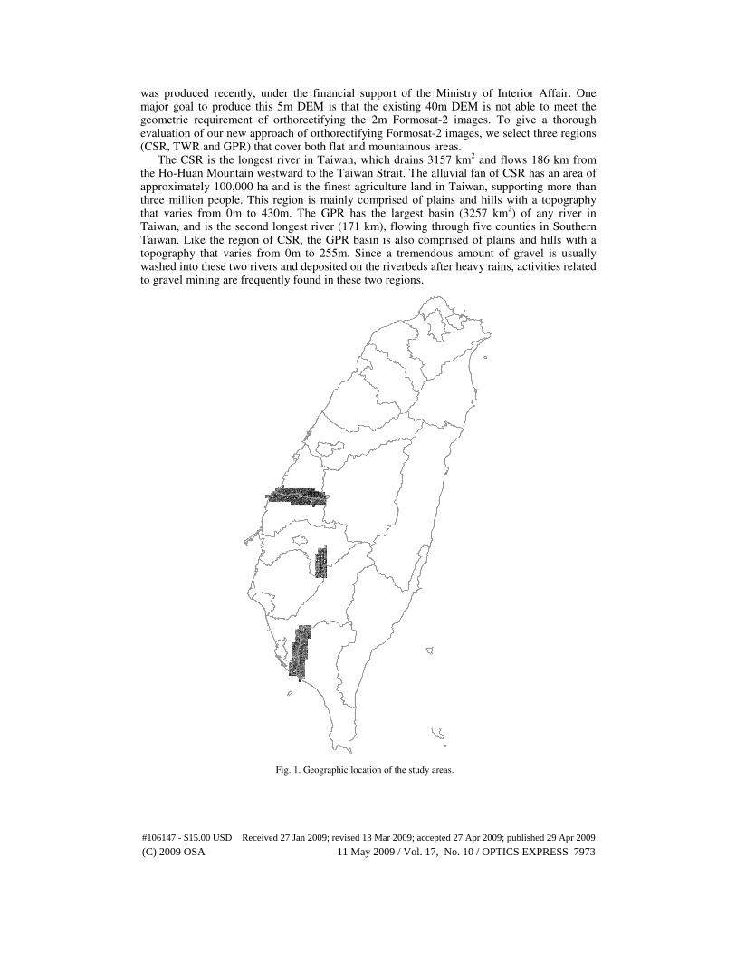
was produced recently, under the financial support of the Ministry of Interior Affair. One major goal to produce this 5m DEM is that the existing 40m DEM is not able to meet the geometric requirement of orthorectifying the 2m Formosat-2 images. To give a thorough evaluation of our new approach of orthorectifying Formosat-2 images, we select three regions (CSR, TWR and GPR) that cover both flat and mountainous areas.

The CSR is the longest river in Taiwan, which drains 3157 km2 and flows 186 km from

the Ho-Huan Mountain westward to the Taiwan Strait. The alluvial fan of CSR has an area of approximately 100,000 ha and is the finest agriculture land in Taiwan, supporting more than three million people. This region is mainly comprised of plains and hills with a topography that varies from 0m to 430m. The GPR has the largest basin (3257 km

2) of any river in

Taiwan, and is the second longest river (171 km), flowing through five counties in Southern Taiwan. Like the region of CSR, the GPR basin is also comprised of plains and hills with a topography that varies from 0m to 255m. Since a tremendous amount of gravel is usually washed into these two rivers and deposited on the riverbeds after heavy rains, activities related to gravel mining are frequently found in these two regions.

Fig. 1. Geographic location of the study areas.



To effectively manage such large areas of CSR and GPR, Formosat-2 imagery has been applied to monitor the illegal quarry mining of gravel on riverbeds on a daily-basis [9]. TWR is the largest water reservoir in Taiwan, which irrigates more than 76,000 km

2 of Chia-Nan

plain and supplies drinking water to 1.2 million people. The entire catchment area of TWR is as high as 481 km

2, yet the small drainage basins are surrounded by hills reaching up to 1,470

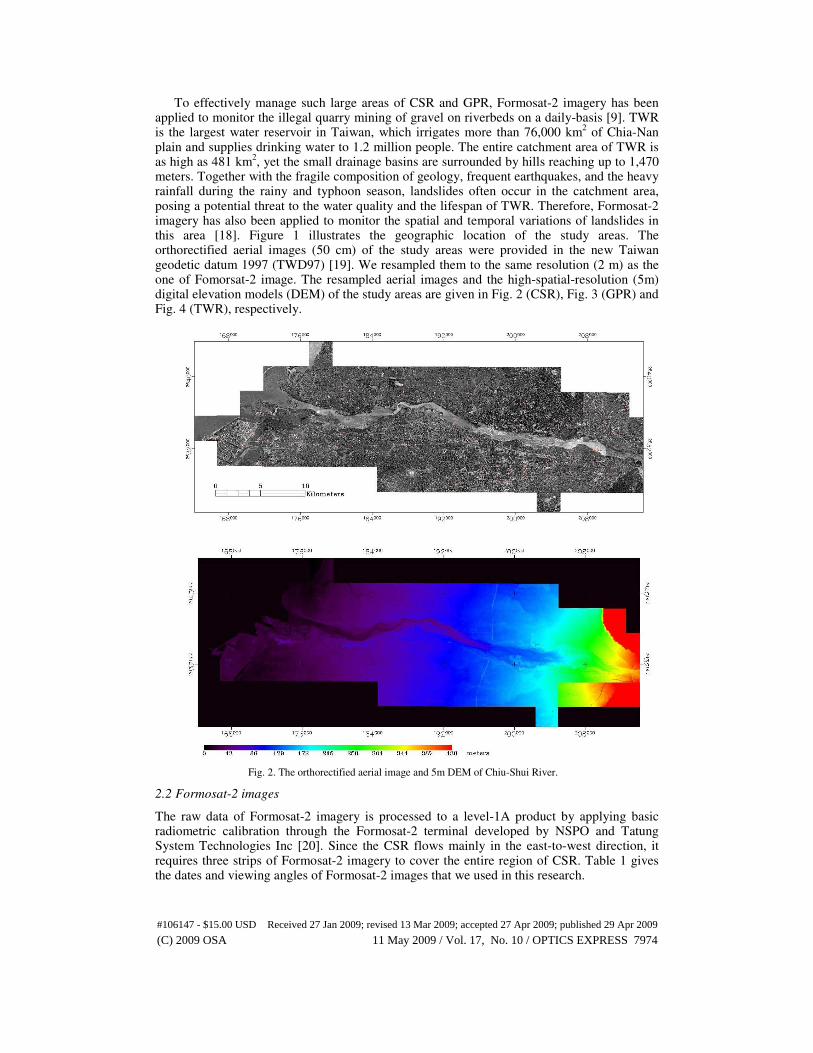
meters. Together with the fragile composition of geology, frequent earthquakes, and the heavy rainfall during the rainy and typhoon season, landslides often occur in the catchment area, posing a potential threat to the water quality and the lifespan of TWR. Therefore, Formosat-2 imagery has also been applied to monitor the spatial and temporal variations of landslides in this area [18]. Figure 1 illustrates the geographic location of the study areas. The orthorectified aerial images (50 cm) of the study areas were provided in the new Taiwan geodetic datum 1997 (TWD97) [19]. We resampled them to the same resolution (2 m) as the one of Fomorsat-2 image. The resampled aerial images and the high-spatial-resolution (5m) digital elevation models (DEM) of the study areas are given in Fig. 2 (CSR), Fig. 3 (GPR) and Fig. 4 (TWR), respectively.

Fig. 2. The orthorectified aerial image and 5m DEM of Chiu-Shui River.

2.2 Formosat-2 images

The raw data of Formosat-2 imagery is processed to a level-1A product by applying basic radiometric calibration through the Formosat-2 terminal developed by NSPO and Tatung System Technologies Inc [20]. Since the CSR flows mainly in the east-to-west direction, it requires three strips of Formosat-2 imagery to cover the entire region of CSR. Table 1 gives the dates and viewing angles of Formosat-2 images that we used in this research.



Fig. 3. The orthorectified aerial image and 5m DEM of Gao-Ping River.

Fig. 4. The orthorectified aerial image and 5m DEM of Tseng-Wen Reservoir.



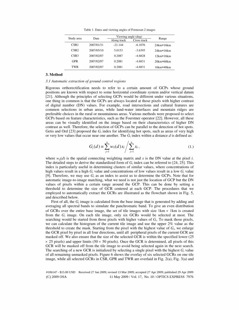
Table 1. Dates and viewing angles of Formosat-2 images

Study area Date Viewing angle (deg)

Range Along track Cross track

CSR1 2007/01/31 -21.144 -6.1076 24km×16km

CSR2 2007/05/10 5.0153 -3.6395 24km×16km

CSR3 2007/02/07 0.2087 -4.6828 12km×16km

GPR 2007/02/07 0.2081 -4.6831 20km×60km

TWR 2007/02/07 0.2081 -4.6831 16km×40km

3. Method

3.1 Automatic extraction of ground control regions

Rigorous orthorectification needs to refer to a certain amount of GCPs whose ground positions are known with respect to some horizontal coordinate system and/or vertical datum [21]. Although the principles of selecting GCPs would be different under various situations, one thing in common is that the GCPs are always located at those pixels with higher contrast of digital number (DN) values. For example, road intersections and cultural features are common selections in urban areas, while land-water interfaces and mountain ridges are preferable choices in the rural or mountainous areas. Various methods were proposed to select GCPs based on feature characteristics, such as the Foerstner operator [22]. However, all these areas can be visually identified on the image based on their characteristics of higher DN contrast as well. Therefore, the selection of GCPs can be parallel to the detection of hot spots. Getis and Ord [23] proposed the Gi index for identifying hot spots, such as areas of very high or very low values that occur near one another. The Gi index within a distance d is defined as:

∑∑==

≡n

j

j

n

j

jiji xxdwdG11

)()( , (1.)

where wij(d) is the spatial connecting weighting matrix and x is the DN value at the pixel i. The detailed steps to derive the standardized form of Gi index can be referred to [24, 25]. This index is particularly useful in determining clusters of similar values, where concentrations of high values result in a high Gi value and concentrations of low values result in a low Gi value [9]. Therefore, we may use Gi as an index to assist us to determine the GCPs. Note that for automatic image-to-image matching, what we need is not just the location of GCP but the DN values of pixels within a certain range around the GCP. This can be done by setting a threshold to determine the size of GCR centered at each GCP. The procedures that we employed to automatically extract the GCRs are illustrated as the flowchart shown in Fig. 5, and described below.

First of all, the Gi image is calculated from the base image that is generated by adding and averaging all spectral bands to simulate the panchromatic band. To give an even distribution

of GCRs over the entire base image, the set of tile images with size 1km × 1km is created from the Gi image. On each tile image, only six GCRs would be selected at most. The searching would be started from those pixels with higher values of Gi. To mask those pixels, we can calculate the histogram of the current tile image and use the upper 2% value as the threshold to create the mask. Starting from the pixel with the highest value of Gi, we enlarge the GCR pixel by pixel in all four directions, until all peripheral pixels of the current GCR are masked off. We also ensure that the size of the selected GCR is within the specified lower (25

× 25 pixels) and upper limits (50 × 50 pixels). Once the GCR is determined, all pixels of this GCR will be masked off from the tile image to avoid being selected again in the next search. The searching of a new GCR is initialized by selecting a single pixel with the highest Gi value of all remaining unmasked pixels. Figure 6 shows the overlay of six selected GCRs on one tile image, while all selected GCRs in CSR, GPR and TWR are overlaid in Fig. 2(a), Fig. 3(a) and



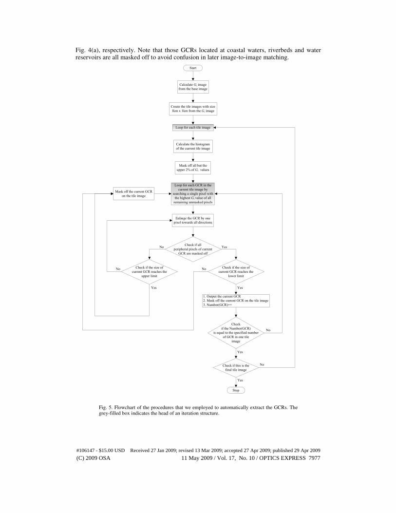
Fig. 4(a), respectively. Note that those GCRs located at coastal waters, riverbeds and water reservoirs are all masked off to avoid confusion in later image-to-image matching.

Calculate Gi image

from the base image

Create the tile images with size

1km x 1km from the Gi image

Loop for each tile image

Calculate the histogram

of the current tile image

Mask off all but the

upper 2% of Gi values

Loop for each GCR in the

current tile image by

searching a single pixel with

the highest Gi value of all

remaining unmasked pixels

Enlarge the GCR by one

pixel towards all directions

Check if all

peripheral pixels of current

GCR are masked off

Check if the size of

current GCR reaches the

lower limit

Check

if the Number(GCR)

is equal to the specified number

of GCR in one tile

image

1. Output the current GCR

2. Mask off the current GCR on the tile image

3. Number(GCR)++

Check if this is the

final tile image

Stop

Start

Yes

No

No

NoNo

Yes

Yes

Check if the size of

current GCR reaches the

upper limit

Mask off the current GCR

on the tile image

Yes Yes

No

Fig. 5. Flowchart of the procedures that we employed to automatically extract the GCRs. The grey-filled box indicates the head of an iteration structure.



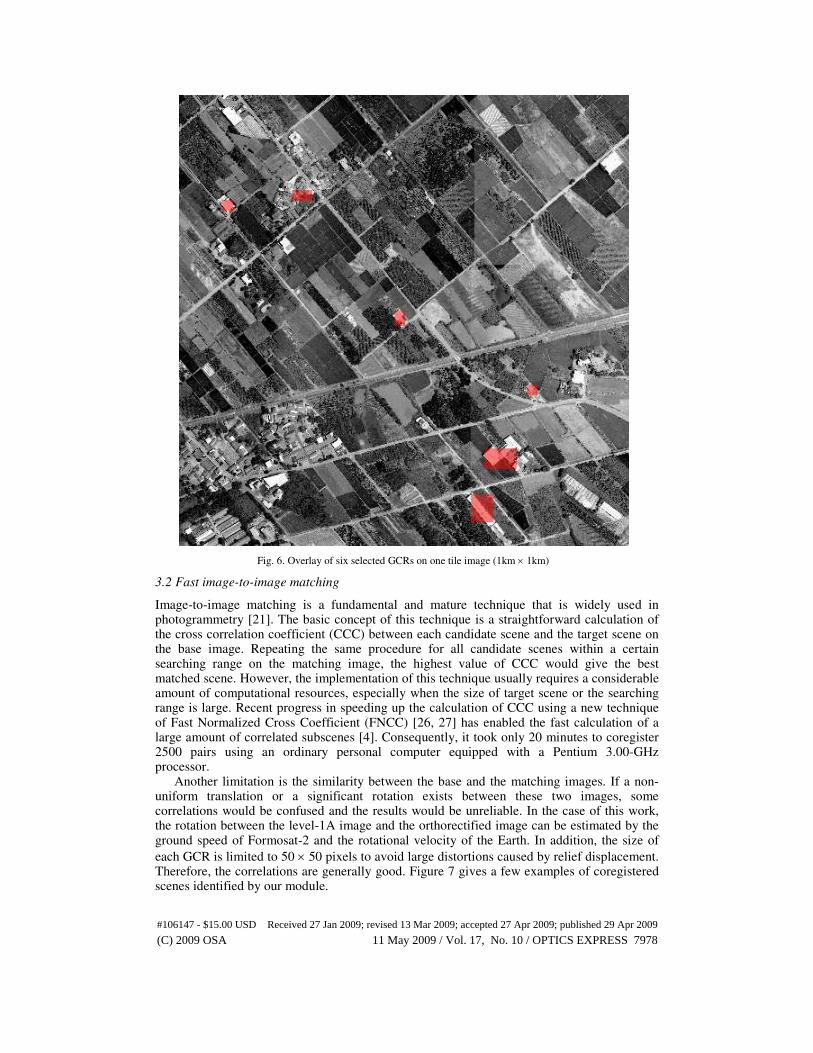
Fig. 6. Overlay of six selected GCRs on one tile image (1km × 1km)

3.2 Fast image-to-image matching

Image-to-image matching is a fundamental and mature technique that is widely used in photogrammetry [21]. The basic concept of this technique is a straightforward calculation of the cross correlation coefficient (CCC) between each candidate scene and the target scene on the base image. Repeating the same procedure for all candidate scenes within a certain searching range on the matching image, the highest value of CCC would give the best matched scene. However, the implementation of this technique usually requires a considerable amount of computational resources, especially when the size of target scene or the searching range is large. Recent progress in speeding up the calculation of CCC using a new technique of Fast Normalized Cross Coefficient (FNCC) [26, 27] has enabled the fast calculation of a large amount of correlated subscenes [4]. Consequently, it took only 20 minutes to coregister 2500 pairs using an ordinary personal computer equipped with a Pentium 3.00-GHz processor.

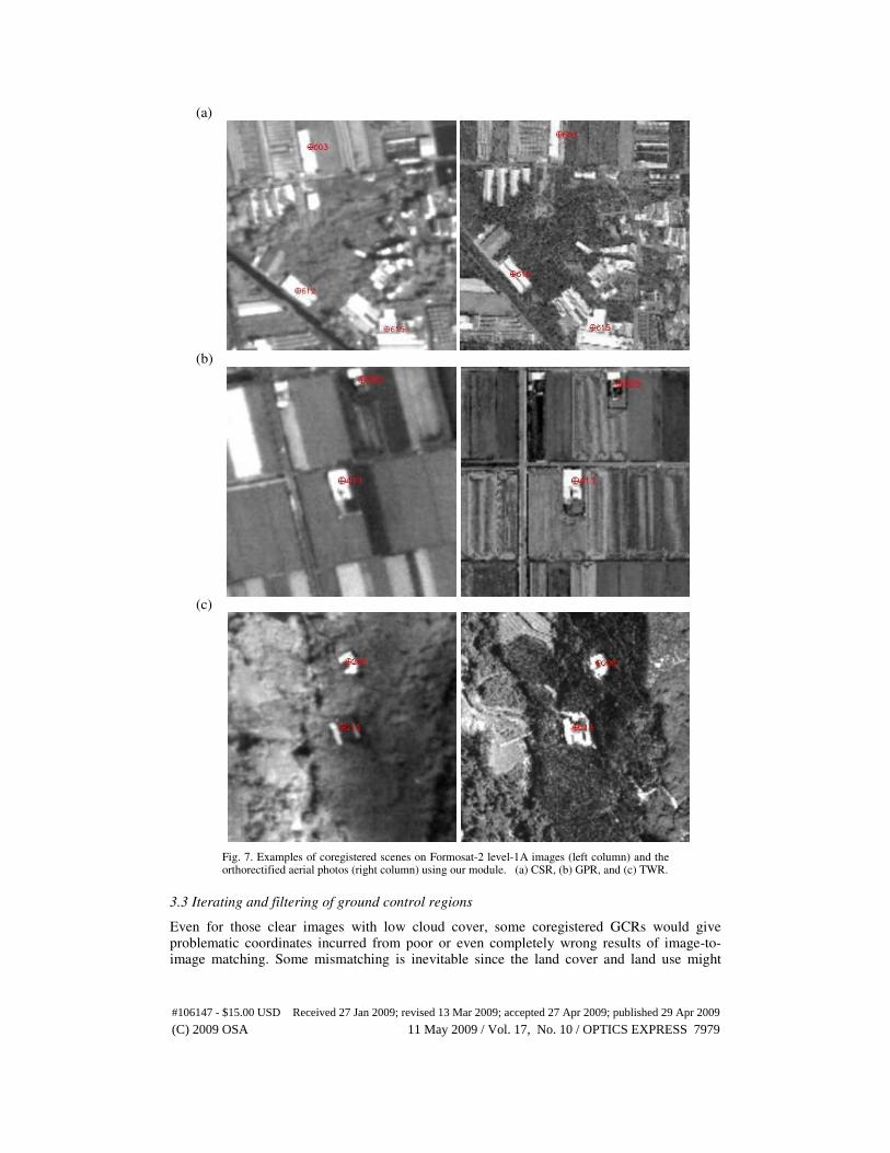
Another limitation is the similarity between the base and the matching images. If a non-uniform translation or a significant rotation exists between these two images, some correlations would be confused and the results would be unreliable. In the case of this work, the rotation between the level-1A image and the orthorectified image can be estimated by the ground speed of Formosat-2 and the rotational velocity of the Earth. In addition, the size of

each GCR is limited to 50 × 50 pixels to avoid large distortions caused by relief displacement. Therefore, the correlations are generally good. Figure 7 gives a few examples of coregistered scenes identified by our module.



(a)

(b)

(c)

Fig. 7. Examples of coregistered scenes on Formosat-2 level-1A images (left column) and the orthorectified aerial photos (right column) using our module. (a) CSR, (b) GPR, and (c) TWR.

3.3 Iterating and filtering of ground control regions

Even for those clear images with low cloud cover, some coregistered GCRs would give problematic coordinates incurred from poor or even completely wrong results of image-to-image matching. Some mismatching is inevitable since the land cover and land use might



have changed significantly between the orthorectified aerial photo and the Formosat-2 level-1A image. This is particularly true if the two images were taken in different seasons. To filter out those problematic GCRs, we assume that most of the coregistered GCRs are accurate and use the transformation model of orthorectification established by all GCRs to get rid of the problematic ones step by step. Note that the assumption is made when the problematic GCR with the highest deviation is filtered out. In other words, all GCRs are assumed to be accurate, except for the one with the highest deviation that is going to be removed. This assumption would be made again in every step of iteration. Since there are still a few hundred GCRs in the final stage of iteration, the assumption is still valid.

The procedure of filtering out the problematic GCRs is as follows: First, a transformation model of rigorous orthorectification is established to examine all correlated GCRs. The GCR with the highest deviation is then removed and a new transformation model is established based on the remaining ones. The iteration is performed until the deviations of all GCRs are less than a specified threshold. Note that the frequency of GPS and INS information onboard Formosat-2 is too low to resolve the dynamic variation of satellite attitude. Therefore, we apply the polynomial-based generic pushbroom model with the interior and exterior orientation parameters acquired from satellite GPS/INS, together with the digital elevation model (DEM) of the imaging area, to establish the transformation model of orthorectification at each iteration. The procedure of filtering out the problematic GCRs is conducted by using the commercial off-the-shelf software, ERDAS Imagine

® 8.7.

3.4 Rigorous orthorectification

Once the problematic GCRs are filtered out, a robust and accurate transformation model of orthorectification can be established. The commercial off-the-shelf software, ERDAS Imagine

® 8.7, is employed again to apply the transformation model to the Formosat-2 level-

1A image, and the orthorectified image is obtained. Note that the problem of band-to-band mis-registration in the original Formosat-2 level-1A image has been fixed by the procedure described in Liu [4] and Liu et al. [8]. This transformation model of orthorectification only needs to be applied to the panchromatic band once. The same geometric correction would be applied to all coregistered multi-spectral bands and the high-quality pan-sharpened image can be obtained automatically.

4. Results and discussion

To assess the accuracy of our new method, we follow the same procedure of analysis used by Baillarin et al. [16] and Habib et al. [17] to measure the mis-registration with the orthorectified aerial image on a random set of check points (CP) by correlation. The CPs are randomly selected subset of the match points established by registering GCRs, and which are not used in adjusting the model parameters. Figures 8 – 10 illustrate the overlay of the error vectors on the Formosat-2 Level-1A images in three study areas. The error vectors are calculated for CPs for each scene. Note that we need three strips of Formosat-2 imagery to cover the entire region of CSR in the east-to-west direction. Table 2 lists the numbers of automatically selected GCRs, filtered GCRs and CPs, as well as the RMSE for each scene. The results show that the RMSEs are generally low for the flat areas CSR1 (1.63), CSR2 (1.53), CSR3 (1.46) and GPR (1.63), and even for the mountainous areas in TWR the RMSEs are no more than 2.17. Note that the accuracy is relative to the geocontrol of the aerial

orthophoto references. It took only four minutes to orthorectify one standard scene (12km × 12km) using an ordinary personal computer equipped with a Pentium 3.00-GHz processor. Compared to the results of similar analysis reported by Baillarin et al. [16] and Habib et al. [17], this research indeed provides a faster and more accurate method that is able to automatically select and match a large amount of ground control points for orthorectifying the high-temporal- and high-spatial-resolution Formosat-2 imagery. This new method has been incorporated into the Formosat-2 automatic image processing system [4] and has been used to produce orthoimages on a daily-basis.



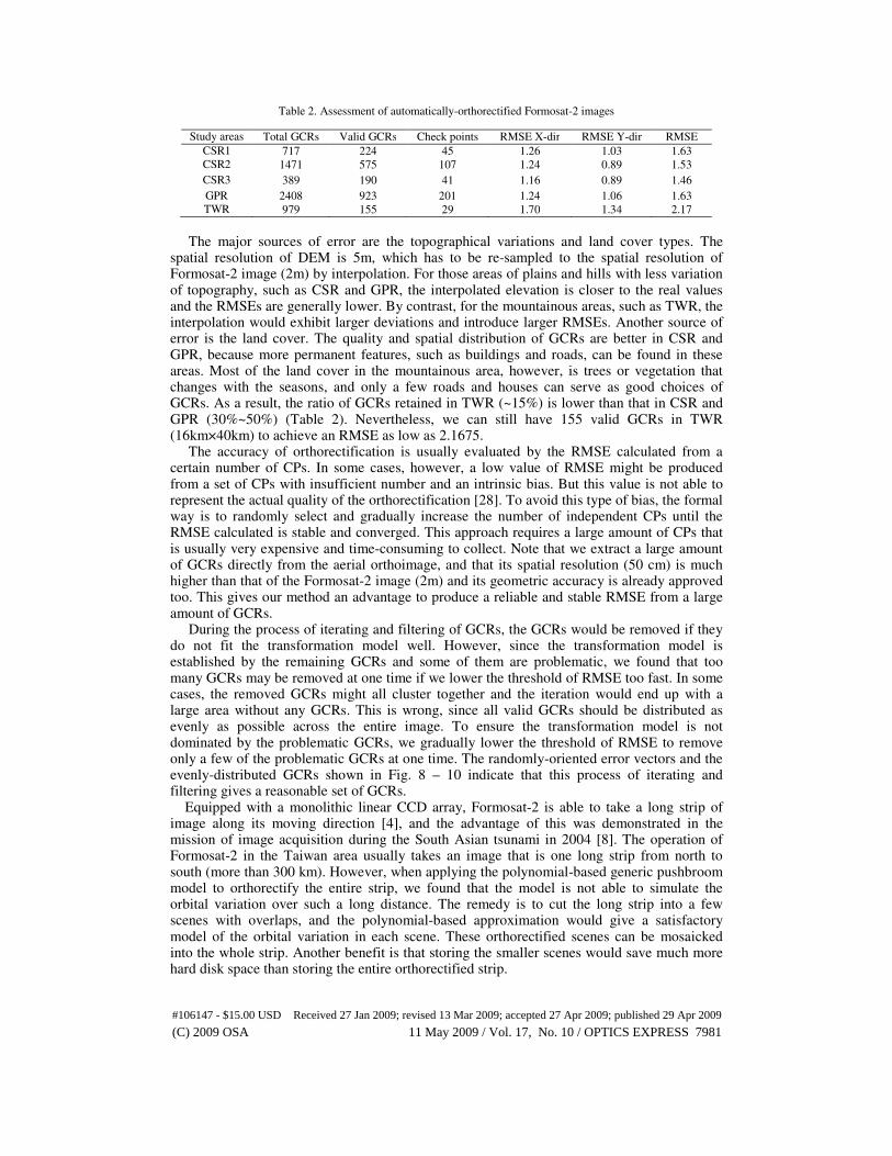
Table 2. Assessment of automatically-orthorectified Formosat-2 images

Study areas Total GCRs Valid GCRs Check points RMSE X-dir RMSE Y-dir RMSE

CSR1 717 224 45 1.26 1.03 1.63

CSR2 1471 575 107 1.24 0.89 1.53

CSR3 389 190 41 1.16 0.89 1.46

GPR 2408 923 201 1.24 1.06 1.63

TWR 979 155 29 1.70 1.34 2.17

The major sources of error are the topographical variations and land cover types. The spatial resolution of DEM is 5m, which has to be re-sampled to the spatial resolution of Formosat-2 image (2m) by interpolation. For those areas of plains and hills with less variation of topography, such as CSR and GPR, the interpolated elevation is closer to the real values and the RMSEs are generally lower. By contrast, for the mountainous areas, such as TWR, the interpolation would exhibit larger deviations and introduce larger RMSEs. Another source of error is the land cover. The quality and spatial distribution of GCRs are better in CSR and GPR, because more permanent features, such as buildings and roads, can be found in these areas. Most of the land cover in the mountainous area, however, is trees or vegetation that changes with the seasons, and only a few roads and houses can serve as good choices of GCRs. As a result, the ratio of GCRs retained in TWR (~15%) is lower than that in CSR and GPR (30%~50%) (Table 2). Nevertheless, we can still have 155 valid GCRs in TWR (16km×40km) to achieve an RMSE as low as 2.1675. The accuracy of orthorectification is usually evaluated by the RMSE calculated from a certain number of CPs. In some cases, however, a low value of RMSE might be produced from a set of CPs with insufficient number and an intrinsic bias. But this value is not able to represent the actual quality of the orthorectification [28]. To avoid this type of bias, the formal way is to randomly select and gradually increase the number of independent CPs until the RMSE calculated is stable and converged. This approach requires a large amount of CPs that is usually very expensive and time-consuming to collect. Note that we extract a large amount of GCRs directly from the aerial orthoimage, and that its spatial resolution (50 cm) is much higher than that of the Formosat-2 image (2m) and its geometric accuracy is already approved too. This gives our method an advantage to produce a reliable and stable RMSE from a large amount of GCRs. During the process of iterating and filtering of GCRs, the GCRs would be removed if they do not fit the transformation model well. However, since the transformation model is established by the remaining GCRs and some of them are problematic, we found that too many GCRs may be removed at one time if we lower the threshold of RMSE too fast. In some cases, the removed GCRs might all cluster together and the iteration would end up with a large area without any GCRs. This is wrong, since all valid GCRs should be distributed as evenly as possible across the entire image. To ensure the transformation model is not dominated by the problematic GCRs, we gradually lower the threshold of RMSE to remove only a few of the problematic GCRs at one time. The randomly-oriented error vectors and the evenly-distributed GCRs shown in Fig. 8 – 10 indicate that this process of iterating and filtering gives a reasonable set of GCRs. Equipped with a monolithic linear CCD array, Formosat-2 is able to take a long strip of image along its moving direction [4], and the advantage of this was demonstrated in the mission of image acquisition during the South Asian tsunami in 2004 [8]. The operation of Formosat-2 in the Taiwan area usually takes an image that is one long strip from north to south (more than 300 km). However, when applying the polynomial-based generic pushbroom model to orthorectify the entire strip, we found that the model is not able to simulate the orbital variation over such a long distance. The remedy is to cut the long strip into a few scenes with overlaps, and the polynomial-based approximation would give a satisfactory model of the orbital variation in each scene. These orthorectified scenes can be mosaicked into the whole strip. Another benefit is that storing the smaller scenes would save much more hard disk space than storing the entire orthorectified strip.



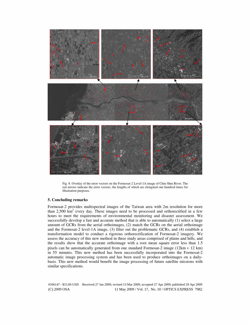
Fig. 8. Overlay of the error vectors on the Formosat-2 Level-1A image of Chiu-Shui River. The red arrows indicate the error vectors, the lengths of which are elongated one hundred times for illustration purposes.

5. Concluding remarks

Formosat-2 provides multispectral images of the Taiwan area with 2m resolution for more than 2,500 km

2 every day. These images need to be processed and orthorectified in a few

hours to meet the requirements of environmental monitoring and disaster assessment. We successfully develop a fast and accurate method that is able to automatically (1) select a large amount of GCRs from the aerial orthoimages, (2) match the GCRs on the aerial orthoimage and the Formosat-2 level-1A image, (3) filter out the problematic GCRs, and (4) establish a transformation model to conduct a rigorous orthorectification of Formosat-2 imagery. We assess the accuracy of this new method in three study areas comprised of plains and hills, and the results show that the accurate orthoimage with a root mean square error less than 1.5

pixels can be automatically generated from one standard Formosat-2 image (12km × 12 km) in 55 minutes. This new method has been successfully incorporated into the Formosat-2 automatic image processing system and has been used to produce orthoimages on a daily-basis. This new method would benefit the image processing of future satellite missions with similar specifications.



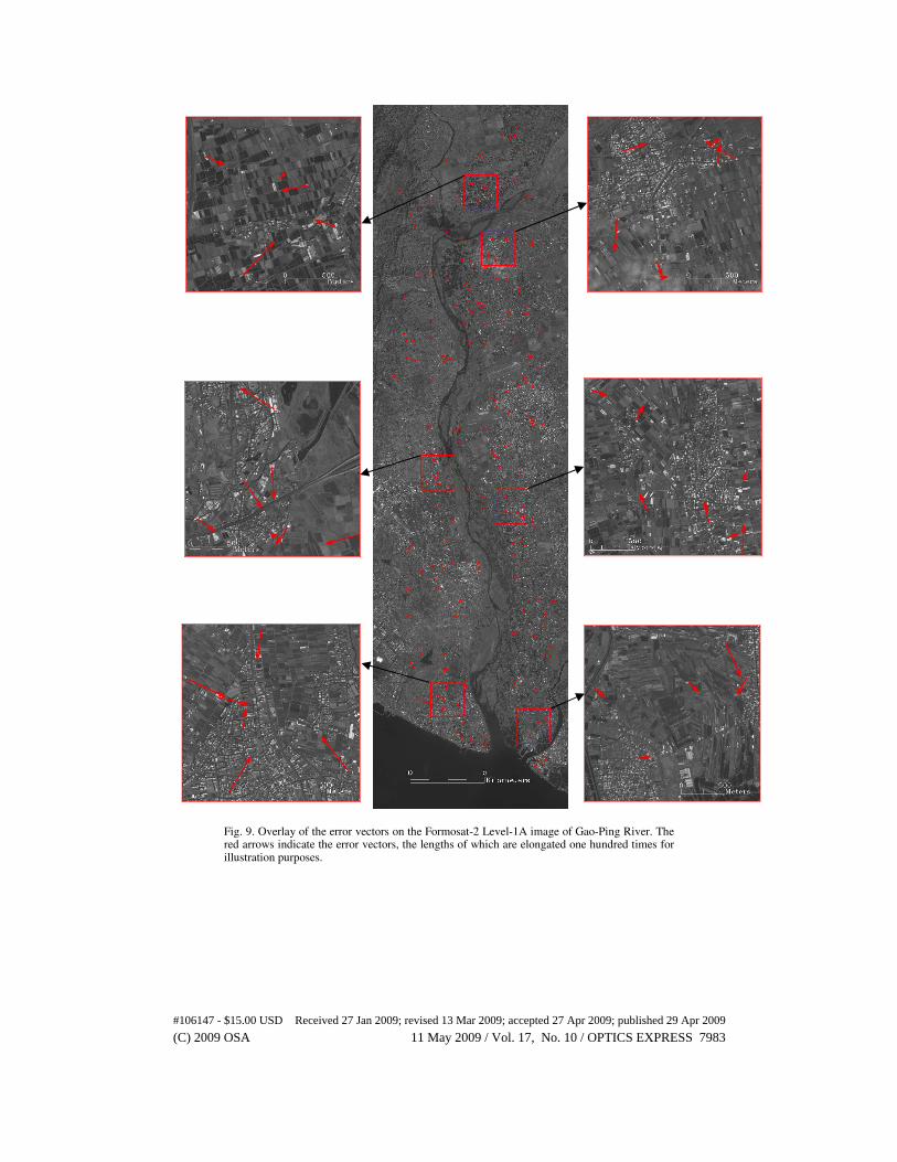
Fig. 9. Overlay of the error vectors on the Formosat-2 Level-1A image of Gao-Ping River. The red arrows indicate the error vectors, the lengths of which are elongated one hundred times for illustration purposes.



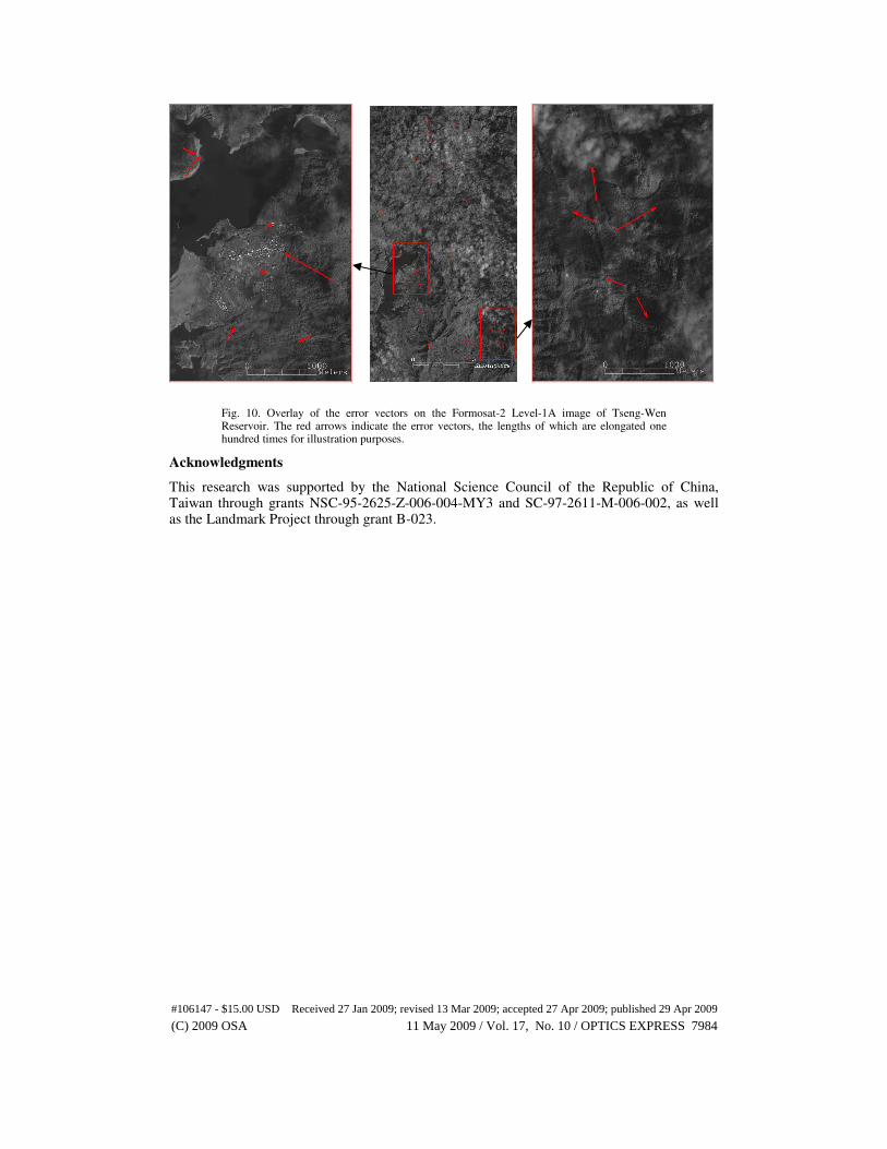
Fig. 10. Overlay of the error vectors on the Formosat-2 Level-1A image of Tseng-Wen Reservoir. The red arrows indicate the error vectors, the lengths of which are elongated one hundred times for illustration purposes.

Acknowledgments

This research was supported by the National Science Council of the Republic of China, Taiwan through grants NSC-95-2625-Z-006-004-MY3 and SC-97-2611-M-006-002, as well as the Landmark Project through grant B-023.



Documents

Automatic extraction of ground control regions and orthorectification of remote sensing imagery