Embed Size (px)
Citation preview

1
AUTOMATIC DETECTION
OF
RWIS SENSOR MALFUNCTIONS
(PHASE II)
FINAL REPORT
Northland Advanced Transportation Systems
Research Laboratories
Project B: Fiscal Year 2006
Carolyn J. Crouch
Donald B. Crouch
Richard M. Maclin
Aditya Polumetla
Department of Computer Science
University of Minnesota Duluth
1114 Kirby Drive
Duluth, Minnesota 55812
2
AUTOMATIC DETECTION OF RWIS SENSOR MALFUNCTIONS
(PHASE II)
Objective
The overall goal of this project (Phases I & II) was to develop computerized procedures that detect
Road Weather Information System (RWIS) sensor malfunctions. In the first phase of the research we
applied two classes of machine learning techniques to data generated by RWIS sensors in order to
predict sensor malfunctions and thereby improve accuracy in forecasting temperature, precipitation,
and other weather-related data. We built models using machine learning (ML) methods that employ
data from nearby sensors in order to predict likely values of those sensor that are being monitored. A
sensor that begins to deviate noticeably from values inferred from nearby sensors serves as an
indication that the sensor has begun to fail. We used both classification and regression algorithms in
Phase I; in particular, we used three classification algorithms: J48 decision trees, naïve Bayes, and
Bayesian networks, and six regression algorithms: linear regression, least median squares (LMS),
M5P, multilayer perceptron (MLP), radial basis function network (RBF), and the conjunctive rule
algorithm (CR). We performed a series of experiments to determine which of these models can be
used to detect malfunctions in RWIS sensors. We compared the values predicted by the various ML
methods to the actual values observed at an RWIS sensor to detect sensor malfunctions.1
Accuracy of an algorithm in predicting values plays a major role in determining the accuracy with
which malfunctions can be identified. From the experiments performed to predict temperature at an
RWIS sensor, we concluded that the classification algorithms LMS and M5P gave results accurate to
±1°F and had low standard deviation across sites. Both models were identified to be able to detect
sensor malfunctions accurately. RBF Networks and CR failed to predict temperature values. A
threshold distance of 2°F between actual and predicted temperature values is sufficient to identify a
sensor malfunction when J48 is used to predict temperature class values. The use of precipitation as
an additional source of decision information produced no significant improvement on the accuracy of
these algorithms in predicting temperature.
The J48, naïve Bayes, and Bayes net exhibited mixed results when predicting the presence or absence
of precipitation. However, a combination of J48 and Bayes nets can be used to detect precipitation
sensor malfunctions, with J48 being used to predict the absence of precipitation and Bayesian
networks, the presence of precipitation. Visibility was best classified using M5P. When the difference
between prediction error and the mean absolute error for M5P is greater than 1.96 standard deviation,
one can reasonably conclude that the sensor is malfunctioning.
In Phase II, we investigated the use of Hidden Markov models to predict RWIS sensor values. The
Hidden Markov model (HMM) is a technique used to model a sequence of temporal events. For
example, suppose we have the sequence of values produced by a given sensor over a fixed time
period. An HMM can be modeled to produce this sequence and then used to determine the probability
of the occurrence of another sequence of values, such as that produced by the given sensor for a
subsequent time period. If the actual values produced by the sensor deviate from the predicted
sequence then a malfunction may have occurred.
1 Detailed information regarding our approach to solving the overall objective of this project is contained in the final report for
Phase I. [1]

3
Hidden Markov Models
A discrete process taking place in the real world generates what can be viewed as a symbol at each
step. For example, the temperature at a given site is a result of existing weather conditions and the
sensor’s location. Over a period of time the process generates a temporal sequence of symbols. Based
on the outcome of the process, these symbols can be discrete (e.g., precipitation type) or continuous
(e.g., temperature). Hidden Markov models may be used to analyze a sequence of observed symbols
and to produce a statistical model that describes the workings of the process and the generation of
symbols over time. Such a model can then be employed to identity or classify other sequences of the
same process.
Hidden Markov models capture temporal data in the form of a directed graph. Each node represents a
state used in recognizing a sequence of events. The arcs between nodes represent a transition
probability from one state to another; probabilities can be combined to determine the probability that
a given sequence will be produced by the HMM. Transitions between states are triggered by events in
the domain. HMM states are referred to as hidden because the system we wish to model may have
underlying causes that cannot be observed. For example, factors that determine the position and
velocity of an object when the only information available is its position are non-observable. The
hidden process taking place in a system can be determined from the events that generate the sequence
of observable events.
State transition networks can be used to represent knowledge about a system. HMM state transition
networks have an initial state and an accepting or end state. The network recognizes a sequence of
events if these events start at the initial state and end in the accepting state. A Markov model is a
probabilistic model over a finite set of states, where the probability of being in a state at a time t
depends only on the previous state visited at time t-1. An HMM is a model where the system being
modeled is assumed to be a Markovian process with unknown parameters.
The components that constitute an HMM are a finite set of states, a set of transitions between these
states and their corresponding probability values, and a set of output symbols emitted by the states.
An initial state distribution gives the probability of being in a particular state at the start of the path.
After each time interval a new state is entered depending on the transition probability from the
previous state. This follows a simple Markov model in which the probability of entering a state
depends only on the previous state. The state sequence obtained over time is called the path. The
transition probability akm of moving from a state k to a state m is given by the probability of being in
state m at time t when at time t-1 we were in state k
akm = P(patht = m | patht-1 = k).
After a transition is made to a new state, a symbol is emitted from the new state. Thus as the state
path is followed we get a sequence of symbols (x1, x2, x3, ...). The symbol which is observed at a state
is based on a probability distribution that depends on the state. The probability that a symbol b is
emitted on transition to state k, called the emission probability (e), is determined by
eb(k) = P(xt = b | patht = k).
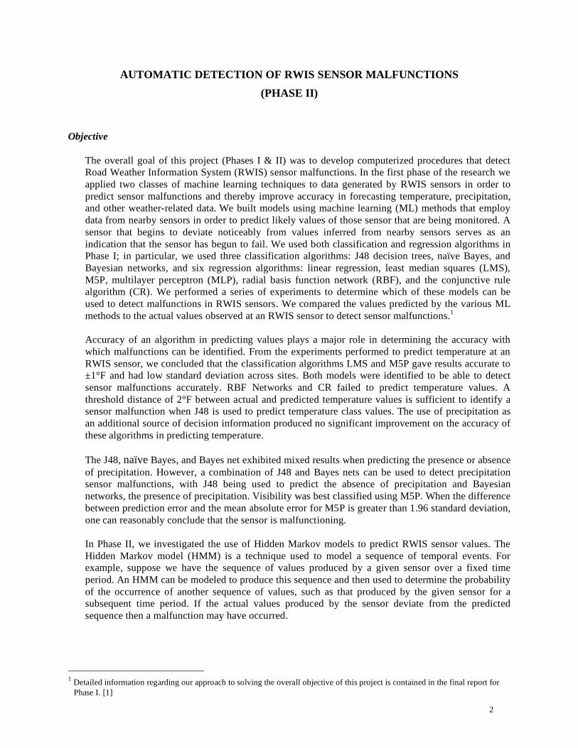
Consider the HMM example in Figure 1 in which there are only three possible output symbols, p, q,
and r, and four states, 1, 2, 3 and 4. In this case our state transition probability matrix will be of size
4x4 and the emission probability matrix will be of size 3 by 4. At each state we can observe any of
the three symbols p, q and r based on their respective emission probabilities at that respective state.
The transition from one state to another is associated with the transition probability between the
respective states. The transition probability of moving from state 1 to state 2 is represented by a12.
Assuming a sequence length of 24, we will observe 24 transitions, including a transition from the start
4
Figure 1: An HMM with four states and three possible outputs
--------------------------------------------------------------------------------------------------------------------------
state and an ending at the end state after the 24th
symbol is seen. The HMM in Figure 1 allows all
possible state transitions.
Rabiner and Juang [2] list three basic questions that have to be answered satisfactorily in order for an
HHM model to be used effectively:
(1) What is the probability that an observed sequence is produced by the given model?
A model can generate many sequences based on the transitions taking place and symbols emitted
each time a state is visited. The probability of the observed sequence being reproduced by the
model gives an estimate of how good the model is; a low probability indicates that this model
probably did not produce it. Forward/Backward algorithms [3] can be used to find the probability
of observing a sequence in a given model.
(2) How do we find an optimal state sequence (path) for a given observation sequence?
HMMs may contain multiple paths that yield a given sequence of symbols. In order to select the
optimal state path, we need to identify the path with the highest probability of occurrence. The
Viterbi algorithm [4,5] is a procedure that finds the single best path in the model for a given
sequence of symbols.
(3) How do we adjust the model parameters, that is, the transition probabilities, emission
probabilities, and the initial state probability, to generate a model that best represents the
training set?
Model parameters need to be adjusted so as to maximize the probability of the observed
sequence. The Baum-Welch algorithm [2] is a method that uses an iterative approach to solve this
problem. It starts with preassigned probabilities and adjusts them dynamically based on the
1
4 3
2
start end
p,q,r
p,q,r
p,q,r
p,q,r
a1e
as4
a4e
as2
a3e
a2e
as3
as1
a13
a31 a42
a24
a21
a12
a34
a43
a23
a32
a32
a23
a11
a33
a22
a44
5
observed sequences in the training set.
The Forward/Backward algorithms, the Baum-Welch algorithm, and the Viterbi algorithm are used
extensively in our development of HMM models. They are relatively efficient algorithms that have
been proposed to solve these three problems. [6] We will describe these algorithms in detail in the
following subsections.
Forward/Backward Algorithms
A sequence of observations can be generated by taking different paths in an HMM model. To find the
probability of a sequence we need to total the probabilities that are obtained for each possible path the
sequence can take. The Forward/Backward algorithms use dynamic programming to calculate this
probability; the major advantage of these algorithms is that all possible paths do not have to be
enumerated.
Since HMMs follow the Markov property, the probability of a path including a particular state
depends only on the state that was entered before it. The Forward Algorithm uses this property to find
the probability of the symbol sequence. Consider an HMM model in which i – 1 symbols in a
sequence x of length L have been observed and the incoming symbol at position i in the sequence is
xi. The probability that symbol xi is in state m can be determined by first summing over all possible
states k the product of two probabilities, the probability of being at any state k when the last symbol
was observed and the transition probability of moving from state k to state m, and then multiplying
this summation result by the emission probability of xi at state m. If a transition is not possible, then
the transition probability is taken as 0. This formula for calculating the probability of observing xi at
position i in state m is referred to as the forward probability and is expressed as
=k
kmkimm aifxeif )1()()( .
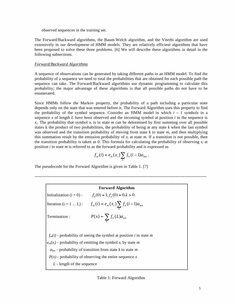
The pseudocode for the Forward Algorithm is given in Table 1. [7]
--------------------------------------------------------------------------------------------------------------------------
Forward Algorithm
Initialization (i = 0) : f0(0) =1; fk (0) = 0,k > 0.
Iteration (i = 1 ... L) : =k
kmkimm aifxeif )1()()(
Termination : =k
kk aLfxP 0)()(
fm(i) - probability of seeing the symbol at position i in state m
em(xi) - probability of emitting the symbol xi by state m
akm - probability of transition from state k to state m
P(x) - probability of observing the entire sequence x
L - length of the sequence
Table 1: Forward Algorithm

6
The Backward Algorithm can also be used to calculate the probability of an observed sequence. It
works analogously to the Forward Algorithm; however, instead of calculating the probability values
from the start state, the Backward Algorithm starts at the end state and moves towards the start state.
In each backward step, it calculates the probability of being at that state taking into account that the
sequence from the current state to the end state has already been observed. The backward probability
bk(i), the probability of observing the remainder of the sequence given that the current state is k after
observing i symbols, is defined as
)|.....()( 1 kpathxxpib iLik == + .
The pseudocode for the Backward Algorithm is given in Table 2. [7] The final probability generated
by either the Forward or Backward algorithm is the same.
Viterbi Algorithm
The Viterbi algorithm is used to find the most probable path taken across the states in an HMM. It
uses dynamic programming and a recursive approach to find the path. The algorithm checks all
possible paths leading to a state and selects the most probable one. Calculations are done using
induction in an approach similar to the forward algorithm, but instead of using a summation, the
Viterbi algorithm uses maximization.
The probability of the most probable path ending at state m, that is, vm(i), after observing the first i
characters of the sequence, is defined as
))((max)1()1( kmkkmm aivieiv +=+ .
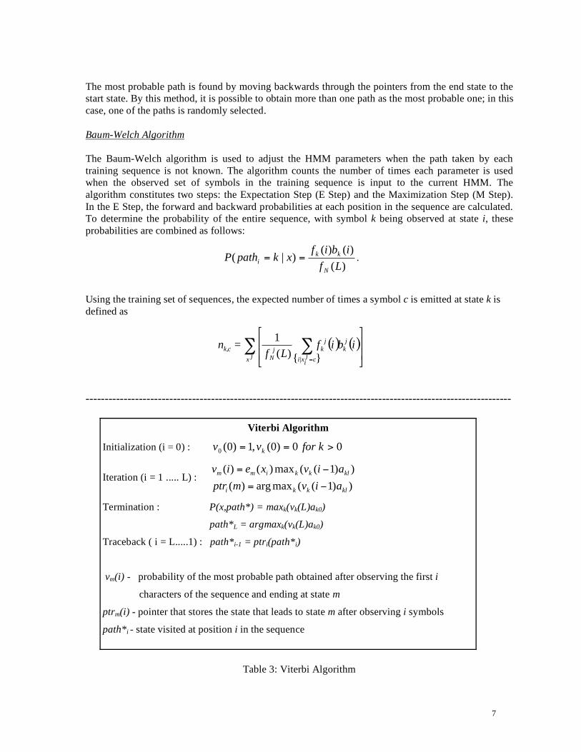
The pseudocode for the Viterbi Algorithm is shown in Table 3. [7] It may be noted that v0(0) is
initialized to 1. The algorithm uses pointers to keep track of the states during a transition. The pointer
ptri(m) stores the state that leads to state m after observing i symbols in the given sequence. It is
determined as follows:
))((maxarg)( kmkki aivmptr = .
----------------------------------------------------------------------------------------------------------------
Backward Algorithm
Initialization (i = L) : kallforaLb kk )( 0=
Iteration (i = L-1 ..... 1) : += +
m
mimkmk ibxeaib )1()()( 1
Termination : =m
mmm bxeaxP )1()()( 10
bk(i) - probability of observing rest of the sequence when in state k and
having already seen i symbols
em(xi) - probability of emitting the symbol xi by state m
akm - probability of transition from state k to state m
P(x) - probability of observing the entire sequence
Table 2: Backward Algorithm
7
The most probable path is found by moving backwards through the pointers from the end state to the
start state. By this method, it is possible to obtain more than one path as the most probable one; in this
case, one of the paths is randomly selected.
Baum-Welch Algorithm
The Baum-Welch algorithm is used to adjust the HMM parameters when the path taken by each
training sequence is not known. The algorithm counts the number of times each parameter is used
when the observed set of symbols in the training sequence is input to the current HMM. The
algorithm constitutes two steps: the Expectation Step (E Step) and the Maximization Step (M Step).
In the E Step, the forward and backward probabilities at each position in the sequence are calculated.
To determine the probability of the entire sequence, with symbol k being observed at state i, these
probabilities are combined as follows:
)(
)()()|(
Lf
ibifxkpathP
N
kk
i == .
Using the training set of sequences, the expected number of times a symbol c is emitted at state k is
defined as
( ) ( )=
jx
j
k
cji
x|i
j
kj
N
ck, ibifLf
=n
}{)(
1
----------------------------------------------------------------------------------------------------------------
Viterbi Algorithm
Initialization (i = 0) : 0 0)0(,1)0(0 >== kforvv k
Iteration (i = 1 ..... L) : ))1((maxarg)(
))1((max)()(
klkki
klkkimm
aivmptr
aivxeiv
=
=
Termination : P(x,path*) = maxk(vk(L)ak0)
path*L = argmaxk(vk(L)ak0)
Traceback ( i = L.....1) : path*i-1 = ptri(path*i)
vm(i) - probability of the most probable path obtained after observing the first i
characters of the sequence and ending at state m
ptrm(i) - pointer that stores the state that leads to state m after observing i symbols
path*i - state visited at position i in the sequence
Table 3: Viterbi Algorithm

8
The number of times a transition from state k to m occurs is given by
+
=
+
jxj
N
i
j
kij
mkm
j
k
mkLf
ibxeaif
n)(
)1()()( 1
,
where the superscript j refers to an instance in the training set.
In order to maximize performance, the Maximization Step uses the number of times a symbol is seen
at a state and the number of times a transition occurs between two states (in the E Step) to update the
transition and emission probabilities. The updated emission probability is
+
+=
'
,,
,,
)'(
')(
c
ckck
ckck
knn
nnce ,
and the transition probability is updated using
+
+=
m
mkmk
mkmk
kmnn
nna
)'(
'.
Pseudo-counts n'k,c and n'k m (emission and transition probabilities, respectively) are taken into
account because it prevents the numerator or denominator from assuming a value of zero which
happens when a particular state is not used in the given set of observed sequences or a transition does
not take place. Table 4 contains the pseudocode of the Baum-Welch algorithm.
In the next section, we describe the data transformation procedures we employed in order to use
Hidden Markov models for weather data modeling. We then describe our approach to the use of
HMMs to as a predictor of RWIS sensor values.
--------------------------------------------------------------------------------------------------------------------------
Baum-Welch Algorithm
Initialize the parameters of HMM and pseudocounts n'k,c and n'k->l
Iterate until convergence or for a fixed number of times
- E Step: for each training sequence j = 1 ... n
calculate the forward probability fk(i) for the sequence j
calculate the backward probability bk(i) for the sequence j
add the contribution of sequence j to nk,c and nk->l
- M Step: update HMM parameters using the expected counts nk,c and nk->l and the
pseudocounts n'k,c and n'k->l.
Table 4: Baum-Welch Algorithm
9
Weather Data Modeling
Minnesota has 91 RWIS meteorological measurement stations positioned alongside major highways
to collect local pavement and atmospheric data. The State is laid out in a fixed grid format and RWIS
stations are located within each grid. The stations themselves are positioned some 60 km apart. Each
RWIS station utilizes various sensing devices, which are placed both below the highway surface and
on towers above the roadway. The sensor data, that is, the variables that will be used in determining
sensor malfunctions, are dependent on the particular type of sensor being evaluated. Each sensor data
item consists of a site identifier, sensor identification, date, time, and the raw sensor values.
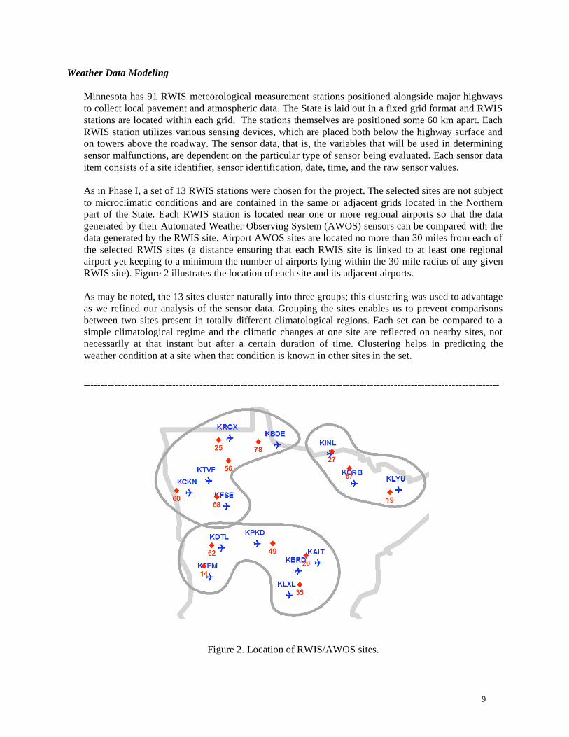
As in Phase I, a set of 13 RWIS stations were chosen for the project. The selected sites are not subject
to microclimatic conditions and are contained in the same or adjacent grids located in the Northern
part of the State. Each RWIS station is located near one or more regional airports so that the data
generated by their Automated Weather Observing System (AWOS) sensors can be compared with the
data generated by the RWIS site. Airport AWOS sites are located no more than 30 miles from each of
the selected RWIS sites (a distance ensuring that each RWIS site is linked to at least one regional
airport yet keeping to a minimum the number of airports lying within the 30-mile radius of any given
RWIS site). Figure 2 illustrates the location of each site and its adjacent airports.
As may be noted, the 13 sites cluster naturally into three groups; this clustering was used to advantage
as we refined our analysis of the sensor data. Grouping the sites enables us to prevent comparisons
between two sites present in totally different climatological regions. Each set can be compared to a
simple climatological regime and the climatic changes at one site are reflected on nearby sites, not
necessarily at that instant but after a certain duration of time. Clustering helps in predicting the
weather condition at a site when that condition is known in other sites in the set.
--------------------------------------------------------------------------------------------------------------------------
Figure 2. Location of RWIS/AWOS sites.

10
Along with the weather information from the RWIS sites, we use meteorological data gathered from
the AWOS sites to help with the prediction of values at an RWIS site. The location of the RWIS sites
with respect to the site's topography is variable, as these sensors sit near a roadway and are sometimes
located on bridges. AWOS sites are located at airports on a flat surrounding topography, which leads
to better comparability between weather data obtained from these sites. Including AWOS information
generally proved beneficial in predicting values at an RWIS site.
Our overall research project focuses on a subset of sensors that includes precipitation, air temperature
and visibility. These sensors were identified by the Minnesota Department of Transportation as being
of particular interest. However, data from other sensors are used to determine if these particular
sensors are operating properly. For HMMs, we concentrated on precipitation and air temperature
since the M5P algorithm performed so well in detecting visibility sensor malfunctions. [1]
RWIS Sensor Data
RWIS sensors report observed values every 10 minutes, resulting in 6 records per hour. Greenwich
Mean Time (GMT) is used for recording the values. The meteorological conditions reported by RWIS
sensors are air temperature, surface temperature, dew point, visibility, precipitation, the amount of
precipitation accumulation, wind speed and wind direction. Following is a short description of these
variables along with the format they follow.
(1) Air Temperature
Air temperature is recorded in Celsius in increments of one hundredth of a degree, with values
ranging from -9999 to 9999 and a value of 32767 indicating an error. For example, a temperature
of 10.5 degree Celsius is reported as 1050.
(2) Surface Temperature
Surface temperature is the temperature measured near the road surface. It is recorded in the same
format as air temperature.
(3) Dew Point
Dew point is defined as the temperature at which dew forms. It is recorded in the same format as
air temperature.
(4) Visibility
Visibility is the maximum distance that it is possible to see without any aid. Visibility reported is
the horizontal visibility recorded in one tenth of a meter with values ranging from 00000 to
99999. A value of -1 indicates an error. For example, a visibility of 800.2 meters is reported as
8002.
(5) Precipitation
Precipitation is the amount of water in any form that falls to earth. Precipitation is reported using
three different variables, precipitation type, precipitation intensity and precipitation rate. A coded
approach is used for reporting precipitation type and intensity. The codes used and the
information they convey are given in Table 5.
The precipitation type gives the form of water that reaches the earth's surface. Precipitation type
with a code of 0 indicates no precipitation, a code of 1 indicates the presence of some amount of
precipitation but the sensor fails to detect the form of the water, a code of 2 represents rain, and
the codes 3, 41 and 42 respectively represent snowfall with an increase in intensity.

11
Code Precipitation Intensity Code Precipitation Type
0 No precipitation 0 None
1 Precipitation detected, not identified 1 Light
2 Rain 2 Slight
3 Snow 3 Moderate
41 Moderate Snow 4 Heavy
42 Heavy Snow 5 Other
6 Unknown
Table 5: RWIS Precipitation Codes
--------------------------------------------------------------------------------------------------------------------------
The precipitation intensity is used to indicate how strong the precipitation is when present. When
no precipitation is present then intensity is given by code 0. As we move from codes 1 to 4 they
indicate an increase in intensity of precipitation. Codes 5 and 6 are used to indicate an intensity
that cannot be classified into any of previous codes and in cases when the sensor is unable to
measure the intensity respectively. A value of 255 for precipitation intensity indicates either an
error or absence of this type of sensor.
Precipitation rate is measured in millimeters per hour with values ranging from 000 to 999 except
for a value of -1 that indicates either an error or absence of this type of sensor.
(6) Precipitation Accumulation
Precipitation accumulation is used to report the amount of water falling in millimeters. Values
reported range from 00000 to 99999 and a value of -1 indicating an error. Precipitation
accumulation is reported for the last 1, 3, 6, 12 and 24 hours.
(7) Wind Speed
Wind speed is recorded in tenths of meters per second with values ranging from 0000 to 9999 and
a value of -1 indicating an error. For example, a wind speed of 2.05 meters/second is reported as
205.
(8) Wind Direction
Wind direction is reported as an angle with values ranging from 0 to 360 degrees. A value of -1
indicates an error.
(9) Air Pressure
Air pressure is defined as the force exerted by the atmosphere at a given point. The pressure
reported is the pressure when reduced to sea level. It is measured in tenths of a millibar and the

12
values reported range from 00000 to 99999. A value of -1 indicates an error. For example, air
pressure of 1234.0 millibars is reported as 12340.
AWOS Sensor Data
AWOS is a collection of systems including meteorological sensors, a data collection system, a
centralized server, and displays for human interaction which are used to observe and report weather
conditions at airports in order to help pilots in maneuvering the aircraft and airport authorities for
proper working of airports and runways. AWOS sensors report values on an hourly basis. The local
time is used in reporting. AWOS sensors report air temperature, dew point, visibility, weather
conditions in a coded manner, air pressure and wind information. Following is a description of these
variables.
(1) Air Temperature
The air temperature value is reported as integer values ranging from -140o F to 140o F.
(3) Dew Point
The dew point temperature is reported in the same format as air temperature.
(4) Visibility
The visibility is reported as a set of values ranging from 3/16 mile to 10 miles. These values can
be converted into floating point numbers for simplicity.
(5) Weather Code
AWOS uses a coded approach to represent the current weather condition. 80 different possible
codes are listed to indicate various conditions. Detailed information about these codes is given in
the document titled “Data Documentation of Data Set 3283: ASOS Surface Airways Hourly
Observations” published by the National Climatic Data Center [NCDC, 2005].
(6) Air Pressure
The air pressure is reported in tenth of a millibar increments. For example, an air pressure of
123.4 millibars is reported as 1234.
(7) Wind Speed and Direction
AWOS encodes wind speed and direction into a single variable. Wind speed is measured in knots
ranging from 0 knots to 999 knots. Wind direction is measured in degrees ranging from 0 to 360
in increments of 10. The single variable for wind has five digits with the first two representing
direction and the last three representing speed. For example, the value for a wind speed of 90
knots and direction of 80 degrees will be 80090.
As noted above, the data format used for reporting RWIS and AWOS sensor values differs. To make
the data from these two sources compatible, the data need to be transformed into a common format. In
some cases, additional preprocessing is necessary in order to discretize the data. We will describe the
data transformation that we utilized in the following subsection.

13
Sensor Data Transformation
RWIS sensors report data every 10 minutes, whereas AWOS provides hourly reports. Thus, RWIS
data needs to be averaged when used in conjunction with AWOS data. The changes that were made to
the RWIS data in order to produce a common format follows.
RWIS uses Greenwich Mean Time (GMT) and AWOS uses Central Time (CT). The
reporting time in RWIS is changed from GMT to CT.
Variables, such as air temperature, surface temperature, and dew point, that are reported in
Celsius by RWIS are converted to Fahrenheit, the format used by AWOS. To convert six
readings per hour to a single hourly reading in RWIS, a simple average is taken.
Distance, which is measured in kilometers by RWIS for visibility and wind speed, is
converted into miles, the format used by AWOS. A single hourly reading is obtained through
a simple average in RWIS.
In order to obtain hourly averages for precipitation type and intensity reported by RWIS, we
use the most frequently reported code for that hour. For precipitation rate, a simple average is
used. RWIS sites report precipitation type and intensity as separate variables, whereas AWOS
combines them into a single weather code. [8] Mapping precipitation type and intensity
reported by RWIS to the AWOS weather codes is not feasible and requires some
compromises to be made. We thus keep these variables in their original format.
Of the three features selected for use in predictions, precipitation type is the one whose direct
comparison between RWIS and AWOS values cannot be done because each uses a different format
for reporting. For broader comparison, we combine all the codes that report different forms of
precipitation, in both RWIS and AWOS, into a single code, which indicates the presence of some
form of precipitation.
Apart from using the features obtained from the RWIS and AWOS sites, we also made use of
historical information to represent our training data. This increases the amount of weather information
we have for a given location or region. We collected hourly temperature values for the 14 AWOS
sites (see Figure 2) from the Weather Underground website2 for a duration of seven years, namely,
1997 to 2004. For many locations, the temperature was reported more than once an hour; in such
cases the average of the temperature across the hour was taken. As we already have readings for
temperature from two different sources, RWIS and AWOS, we use the information gathered from the
website to adjust our dataset by deriving values such as the projected hourly temperature. To calculate
the projected hourly temperatures for an AWOS site we use past temperature information obtained
from the website for this location. The projected hourly temperature for an hour of a day is defined as
the sum of the average temperature reported for that day in the year and the monthly average
difference in temperature of that hour in the day for the respective month.
The steps followed to calculate the projected hourly temperature for an AWOS site are as follows:
Obtain the hourly temperature for the respective AWOS site.
Calculate the average temperature for a day as the mean of the hourly readings across a day.
Calculate the hourly difference as the difference between the average daily temperature and
actual temperature seen at that hour.
Calculate the average difference in temperature per hour for a particular month (monthly
average difference) as the average of all hourly differences in a month for that hour obtained
2.
http://www.wunderground.com/

14
from all the years in the data collected.
Calculate the projected hourly temperature for a day from the sum of the average temperature
for that day and the monthly average difference of that hour in the day.
For example, suppose the temperature value at the AWOS site KORB for the first hour for January 1st
for year 1997 is 32ºF. The temperature values for all 24 hours on January 1st are averaged; assume
this value is 30ºF. The hourly difference for this day for the first hour will be 2ºF. Now assume the
average of all the first hourly differncee values for the month of January for KORB from years 1997
to 2004 is 5ºF. Then the projected temperature value for the first hour in January 1st, 1997 will be
35ºF, which is the sum of the average temperature seen on January 1st 1997 and the monthly average
difference for the first hour in the month of January.
The projected hourly temperature was used as a feature in the datasets used for predicting weather
variables at an RWIS site and is also used in the process of discretizing temperature.
Discretization of the Data
Hidden Markov Models require the data to be discrete. If the data is continuous, discretization of the
data involves finding a set of values that split the continuous sequence into intervals; each interval is
then assigned a single discrete value.
Discretization can be accomplished using unsupervised or supervised methods. In unsupervised
discretization, the data is divided into a fixed number of equal intervals, without any prior knowledge
of the target class values of instances in the given dataset. In supervised discretization, the splitting
point is determined at a location that increases the information gain with respect to the given training
dataset. [9] Dougherty [10] gives a brief description of the process and a comparison of unsupervised
and supervised discretization. WEKA [11] provides a wide range of options to discretize any
continuous variable, using supervised and unsupervised mechanisms.
We propose a new method for discretization of RWIS temperature sensor values that uses data
obtained from other sources. Namely, using the projected hourly temperature for an AWOS site along
with the current reported temperature for the closest RWIS site, we determine a class value for the
current RWIS temperature value. The actual reported temperature at an RWIS site is subtracted from
the projected hourly temperature for the AWOS site closest to it for that specific hour. This difference
is then divided by the standard deviation of the projected hourly temperature for that AWOS site. The
result indicates how much the actual value deviates from the projected value, that is, the number of
standard deviation from the projected value (or the mean):
num_stdev = (actual_temp – proj_temp) / std_dev
The number of standard deviations determines the class that the temperature value is assigned, as
shown in Table 6. The ranges and the number of classes can be determined by the user or based on
requirements of the algorithm.
For example, to convert the actual temperature of 32ºF at an RWIS site, we calculate the projected
temperature for that hour at the associated AWOS site, say 30ºF, and the standard deviation of
projected temperatures for the year, 5.06. This yields a value of 0.395 as the number of standard
deviations from the mean. Thus the representation for 32ºF is assigned to be class 6. The advantage of
determining classes in this manner is that the effect of season and time of day is at least partially
removed from the data.

15
Class Value Class Value
1 num_stdev < -2 6 0.25 < num_stddev 0.5
2 -2 num_stdev -1 7 0.5 < num_stddev 1
3 -1 < num_stdev -0.5 8 1 < num_stddev 2
4 -0.5 < num_stdev -0.25 9 num_stdev > 2
5 -0.25 < num_stdev 0.25
Table 6: RWIS Temperature Classes
--------------------------------------------------------------------------------------------------------------------------
Feature Vectors
To build models that can predict values reported by an RWIS sensor, we require a training set and a
test set that contain data related to the weather conditions. Each member of these sets is represented
by a so-called feature vector for the dataset consisting of a set of input attributes and an output
attribute, with the output attribute corresponding to the RWIS sensor of interest. The input attributes
for a feature vector in the test set are applied to the model built from the training set to predict the
output attribute value. This predicted value is compared with the sensor’s actual value to estimate
model performance. The feature vector has the form
input1, ...., inputn, output
where inputi is an input attribute and output is the output attribute.
The performance of a model is evaluated using cross-validation. The data is divided repeatedly into
training and testing groups using 10-fold cross validation, repeated 10 times. In 10-fold cross
validation the data is randomly permuted and then divided into 10 equal sized groups. Each group is
then in turn used as test data while the other 9 groups are used to create a model (in this way every
data point is used as a test point exactly once). The results for the ten groups are summed, and the
overall result for the test data is reported.
Predicting a value for an RWIS sensor corresponds to predicting the weather condition being reported
by that sensor. Since variations in a weather condition, like air temperature, are dependent to some
degree on other weather conditions, such as wind, precipitation, and air pressure, many different types
of sensors are used to predict a single sensor’s value at a given location. Earlier readings (such as
those during the previous 24 hour period) from a sensor can be used to predict present conditions, as
changes in weather conditions follow a pattern and are not totally random. In addition, as noted in
Figure 2, we divided the RWIS-AWOS sites into clusters. Any site within a single cluster is assumed
to have climatic conditions similar to any other site in the cluster. This assumption allows us to use
both RWIS and AWOS data obtained from the nearby sites (those in the same cluster) to predict
variables at a given RWIS site in the cluster.
In Hidden Markov models the instance in a dataset used for predicting a class value of a variable
consists of a string of symbols that form the feature vector. The symbols that constitute the feature
16
vector are unique and are generated from the training set. Predicting a weather variable value at an
RWIS site that is based on hourly readings for a day yields a string of length 24. This string forms the
feature vector which is used in the dataset.
When information from a single site is used for predictions, the class values taken by the variables
form the symbol set. When the variable information from two of more sites is used together, a class
value is obtained by appending the variable's value from each site together. For example, to predict a
temperature class of site 19 using the Northeast cluster in Figure 2, we include temperature data from
sites 27 and 67. The combination of class values from these three sites for a particular hour will form
a class string. For example if the temperature class values at sites 19, 27, and 67 are 3, 5, and 4,
respectively, then the class string formed by appending the class values is 354.
The sequence of hourly class strings for a day form an instance in the dataset. All unique class strings
that are seen in the training set are arranged in ascending order, if possible, and each class string is
assigned a symbol. For hourly readings taken during a day we arrive at a string which is 24 symbols
long, which forms the feature vector used by the HMM.
Hidden Markov Approach
To build an HMM model from a given number of states and symbols, the Baum-Welch algorithm is
first applied to the training set to determine the initial state, transmission probabilities, and emission
probabilities. Each symbol generated using the training set is emitted by a state. Instances from the
test set are then passed to the Viterbi algorithm which yields the most probable state path.
To predict a variable’s class value, we need the symbol that would be observed across the most
probable state path found by the Viterbi algorithm. In order to obtain such symbols, we had to modify
the Viterbi algorithm. Table 7 contains the modified algorithm. The algorithm works similarly to the
original algorithm (Table 3). It calculates the probability of the most probable path obtained after
observing the first i characters of the given sequence and ending at state m using
))1((max)()( kmkkimm aivxeiv = ,
where em(xi) is the emission probability of the symbol at state m and akm is the transition probability of
moving from state k to state m. However, in the modified Viterbi algorithm, in place of em(xi) we use
the emission probability value that is the maximum of all of the possible symbols that can be seen at
state m when the symbol xi is present in the actual symbol sequence. We calcualte vm(i) in the
modified Viterbi algorithm as
))((max*))1((max)( smskmkkm symbolseteaiviv = .
The actual symbol seen in the symbol string for that respective time is taken and all its possible
symbols are found. Of the possible symbols or class strings, only those that are seen in the training
instances are considered in the set of possible symbols. The symbol from the set of possible symbols
that has the highest emission probability is selected as the symbol observed for the given state. To
retain the symbol that was observed at a state, the modified Viterbi algorithm uses the pointer
bestsymboli(m) which contains the position of the selected symbol in the set of possible symbols seen
at state m for a position i in the sequence. It is given by
))((maxarg)( smsi symbolsetembestsymbol = .

17
Modified Viterbi Algorithm
Initialization (i = 0) : 0 0)0(,1)0(0 >== kforvv k
Iteration (i = 1 ..... L) :
))((maxarg)(
))1((maxarg)(
))((max*))1((max)(
)(
smsi
klkki
smskmkkm
i
symbolsetembestsymbol
aivmptr
symbolseteaiviv
xesymbolsallpossiblsymbolset
=
=
=
=
Termination : P(x,path*) = maxk(vk(L)ak0)
path*L = argmaxk(vk(L)ak0)
Traceback ( i = L.....1) : path*i-1 = ptri(path*i)
Symbol Observed ( i = 1 ... L): symbol(i) = bestsymboli ( path*i )
vm(i) - probability of the most probable path obtained after observing the
first I characters of the sequence and ending at state m
ptrm(i) - pointer that stores the state that leads to state m after
observing i symbols
path*i - state visited at position i in the sequence
bestsymboli(m) - the most probable symbol seen at state m at position in
the sequence
symbolsets – the set of all possible symbols that can be emitted from a state
when a certain symbol is actually seen
allpossibesymbols(xi) – function that generates all possible symbols for the
given symbol xi.
symbol(i) – symbol observed ith position in the string.
Table 7: Modified Viterbi Algortihm
--------------------------------------------------------------------------------------------------------------------------
The most probable path generated by the algorithm is visited from the start, and by retaining the
symbols that were observed at the state for a particular time, we can determine the symbols with the
highest emission probability at each state in the most probable state path. This new symbol sequence
gives the observed sequence for that given input sequence; in other words, it is the predicted sequence
for the given actual sequence.
To predict the class values for a variable at an RWIS site for a given instance, we pass the instance
through the modified Viterbi algorithm which then gives the symbols that have the highest emission
probabilities along the most probable path. The symbol found is then converted back into a class
string, and the class value for the RWIS site of interest is regarded as the predicted value.

18
For example, to predict temperature class values at site 19 in Figure 2, we use the class string for
temperature class values from sites 27 and 67 appended to the value observed at site 19. Suppose the
class string sequence for a given day is
343, 323, 243, 544, … , 324
a feature vector of length of 24, one for each hour in a day. This sequence is passed to the modified
Viterbi algorithm which yields the observed sequence along with most probable state path. Now
suppose the output sequence for the given sequence is
433, 323, 343, 334, … , 324
As we are interested in predicting the class values at site 19, taking only the first class value from a
class string we get for actual values
3, 3, 2, 5, … , 3
The observed (or predicted) values for the day are
4, 3, 3, 3, … , 3
The distance between these class values gives the accuracy of the predictions made by the model.
The performance of the HMM on the given test set, on precipitation type and discretized temperature,
can be evaluated using the same methods that were used in the general classification approach used in
Phase 1. [1]
Empirical Analysis
Based on the instance given, an HMM tries to predict the most probable path taken across the states.
For weather data the path is the predicted values of the weather sensor using the surrounding sensors
for additional information. HMMs can be used to classify discrete attributes. When data is present in
the form of a time series, such as hourly precipitation, HMMs can be used to identity the path of
predicted values from which we can further obtain the values observed through the path.
We used the modified Viterbi algorithm to predict the symbol observed when a state in the most
probable path is reached for the given instance. HMMs require a training dataset to build the model,
that is, to estimate the initial state, transition probabilities, and emission probabilities. The test dataset
was used to evaluate the model. Multiple n-fold cross-validation was used to estimate model
performance. As HMMs require the presence of all symbols in the symbol sequence, any time
sequence with missing data (due to a sensor not reporting or transmission problems) was omitted
from the dataset used for predictions.
HMMs require class value information. For the RWIS sites that were used for predictions, we
discretized the temperature following the method previously described; namely, the temperature was
broken down into nine classes based on the value obtained for the number of standard deviations the
actual temperature value differs from the predicted value (Table 6). For nearby sites, we used a
broader classification of temperature values, as shown in Table 7; such sites required less precise
differentiation since they are providing additional information for making predictions. For example,
to predict temperature values at site 19, we used temperature values of the nearby sites 27 and 67 for
additional information. Each temperature value at site 19 was represented as one of nine possible
classes and temperatures at sites 27 and 67 were chosen as one of five classes.

19
Class Value Class Value
1 num_stdev < -1 4 0.5 < num_stdev 1
2 -1 num_stdev -0.5 5 num_stdev > 1
3 -0.5 < num_stdev -0.5
Table 8: RWIS Temperature Classes for Nearby Sites
--------------------------------------------------------------------------------------------------------------------------
In the following experiments, we trained the Hidden Markov Model using the methods available in
the HMM Toolbox for MATLAB developed by Murphy [12]. The modified Viterbi algorithm was used
for testing. We performed ten iterations of the Baum-Welch algorithm during the training of the
HMM. We set the number of states in the model to 24 and each state was allowed to emit all possible
symbols obtained from the training set. Since we are using hourly readings for a day, each instance in
the dataset is a string of symbols with a length of 24.
Training the HMM
Two different methods were devised to train the HMMs to predict the temperature class value
reported at an RWIS site. The temperature class information from the RWIS site and the other RWIS
sites in its group are used to form the feature symbols. The results obtained from predicting
temperature class value were used to compare the two methods.
(1) Method A
In this approach we merged all the data from a group and trained the HMM using this data. As
noted earlier, the site being used for prediction has 9 temperature classes (Table 6) and the other
sites in the group have 5 temperature classes (Table 8). Thus, each site has its own merged
dataset.
We create the dataset in which each instance is a string of symbols representing hourly readings
per day, where a symbol for an hour was obtained from appending that hour's temperature class
value for all of the RWIS sites in a group together. For example to predict temperature class
values at site 19, we used the temperature classes from sites 27 and 67. If the temperature class
values at time t seen at sites 19, 27 and 67 are 6, 3 and 2 then the class string generated for time t
will be 632. We estimated the initial state, transition, and emission probabilities by applying the
Baum-Welch algorithm on this dataset with combined class information.
(2) Method B
In this approach the data from the sites used is not merged. Instead, data from each site is used for
training the model, and the emission probabilities of all sites in the group are multiplied to obtain
a single emission matrix for the final model.
We created a separate dataset for each RWIS site in which each instance is a string of symbols
representing hourly temperature class value per day. We applied the Baum-Welch algorithm to the
dataset for the RWIS sites to estimate the initial state, transition probabilities, and emission

20
probabilities. The emission probability matrices obtained for each RWIS site in a group were then
joined together by multiplying the respective values in each cell in the matrix. The resultant emission
matrix was made stochastic, that is, such the sum of all rows and columns is 1. In order to increase
probabilities with small values, we applied the m-estimate to the probability values in the matrix,
using a value of 20 for m and the inverse of the number of classes as the value of p. In this case the
number of classes denotes the total number of class values taken by the variable we are trying to
predict. By applying the m-estimate, we get new values in each cell of the matrix as defined by
matrix(row.col) = (matrix(row,col) + mp) / (1 + m)
We used the initial state and transition probabilities for the RWIS site whose temperature value is to
be predicted in the model. We used the temperature values at the RWIS sites for the years 2002 and
2003 in the training set while the test set contained temperature information from January 2004 to
April 2004. We discretized the temperature values by allocating them into nine classes. Training was
done using the two methods mentioned above, and temperature class value was predicted for
instances in the test data using the modified Viterbi algorithm.
Results
We used the absolute distance between the actual and predicted class values for temperature as a
measure to estimate the performance of the algorithm. Figure 3 shows the percentage of instances in
the training set for each distance between the actual and predicted class averaged across the results
from different RWIS sitea. The HMM was trained using Method A and Method B. A distance of
zero indicates a perfectly classified instance.
--------------------------------------------------------------------------------------------------------------------------
0.00%
10.00%
20.00%
30.00%
40.00%
50.00%
60.00%
0 1 2 3 4 5 6 7 8
Distance
Pe
rce
nta
ge
of
Ins
tan
ce
s
Method A
Method B
Figure 3. Percentage of Instances in Test Set with Differences between Actual and Predicted Values.
21
Smaller distances between the actual and predicted values indicate more accuracy in predictions.
From Figure 3 we can observe that Method A classified more instances with distance 1 or less,
whereas Methods 2 had comparatively fewer number of instances classified with distance below 2.
This indicates that Method A outperforms Method B. Consequently, we elected to use Method A for
training the HMM to predict sensor malfunctions in the experiments that follow.
Predicting Temperature
In this experiment we attempt to predict the temperature class value reported at an RWIS site. The
temperature class information from the RWIS site and the other RWIS sites in its group are used to
form the feature symbols.
Using temperature data collected for each RWIS site, ranging from January 2002 to April 2004, we
created a dataset for each RWIS site to be used for predictions. In this dataset each instance is a string
of symbols representing hourly readings for a day, where a symbol for an hour was obtained by
appending that hour's temperature class value for all RWIS sites in a group. In each class string the
RWIS site predicted was listed first and the other sites in the group were added in order of their
nautical distance from the RWIS site of interest. This order is useful for finding the closest symbol
when a class string in the test set is missing from the training set used. We estimated the performance
of HMM in predicting the current hour's temperature class value at an RWIS site using the dataset of
the group this site belonged to and applied a single 10-fold cross-validation to estimate the model
evaluation.
We evaluated the performance of the HMM using the absolute distances between the actual and
predicted values. The respective distance values for all RWIS sites in a group were averaged so as to
reflect on the performance of the HMM in predicting temperature class values for that respective set.
We do not combine the results of different sets to reach an overall percentage value, since the format
of the symbol sequence in a dataset is different for each site. Figure 4 shows the percentage values for
each distance for the three sets, with the percentage calculated as the number of instances classified
with a certain distance over the total instances present in the dataset, with each instance being an
hourly reading. The percentage for each distance across all the RWIS sites used for prediction is
detailed in the Appendix.
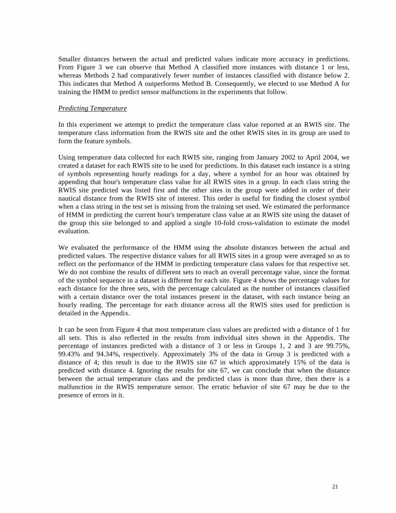
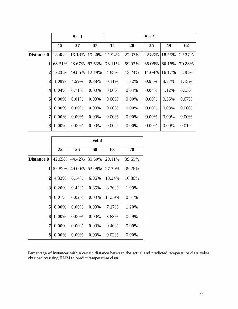
It can be seen from Figure 4 that most temperature class values are predicted with a distance of 1 for
all sets. This is also reflected in the results from individual sites shown in the Appendix. The
percentage of instances predicted with a distance of 3 or less in Groups 1, 2 and 3 are 99.75%,
99.43% and 94.34%, respectively. Approximately 3% of the data in Group 3 is predicted with a
distance of 4; this result is due to the RWIS site 67 in which approximately 15% of the data is
predicted with distance 4. Ignoring the results for site 67, we can conclude that when the distance
between the actual temperature class and the predicted class is more than three, then there is a
malfunction in the RWIS temperature sensor. The erratic behavior of site 67 may be due to the
presence of errors in it.

22
Figure 4. % of Instances with Differences between Actual and Predicted Temperature Values
-------------------------------------------------------------------------------------------------------------------------------
Site Independent Prediction of Temperature
This experiment evaluates the use of HMMs to predict the temperature class value reported for a site
in a given RWIS grouping. A single dataset was generated for the group with the first class value in
the class string representing the class value to be predicted. The temperature class information from
the RWIS sites in a group are used to form the feature symbols.
In order to increase the size of data used for predictions and to perform site independent predictions,
we created a single dataset for each RWIS group. Each of the RWIS sites in a group was taken as the
predicted site, and the symbol strings obtained from it were appended to the dataset. The class string
was constructed using the predicted site's class value as the first component followed by the class
values of the other sites in the group. Ordering of the nearby sites was done with respect to the
distance from the predicted site; the site closest to the predicted site was added first and so on. For
example, to create a single dataset for RWIS Group 1, we first add data instances taking RWIS site 19
as the site to be predicted, with sites 27 and 67 as nearby sites, followed by taking site 27 to be the
site predicted and then using site 67 as the site predicted. This process yields a single large dataset
whose size is equal to the sum of the sizes of the datasets generated for each site in an RWIS group.
By predicting the first class seen in the dataset, we perform a site independent evaluation of the HMM
that focuses on prediction accuracy within a group.
A dataset was generated for each group using the temperature data from the years 2002 and 2003. It
was used to predict the first class value (the predicted site) seen in the class string using HMMs, and
the model was evaluated using ten 10-fold cross validation runs. The distance between actual and
predicted class value was used to evaluate the performance of the model.
0.00%
10.00%
20.00%
30.00%
40.00%
50.00%
60.00%
70.00%
0 1 2 3 4 5 6 7
Distance
Pe
rce
nta
ge
of
Insta
nces
Group 1: RWIS Sites 19, 27 and 67
Group 2: RWIS Sites 14, 20, 35, 49 and 62
Group 3 :RWIS Sites 25, 56, 60, 68 and 78

23
Figure 5 shows the percentage of instances (with an instance being an hourly reading) having a given
distance between each of the three RWIS sets. The percentage values were obtained after averaging
the values reported for each cross-validation run. Comparing the results of the previous experiment
with these results, we observe from Figures 4 and 5 that the percentage of instances with a given
distance is almost the same. In other words, the results obtained for a group using a combined dataset
and for averaging results from within a group where each site was trained using its dataset are almost
identical. Thus we can conclude that using a single model built from the combined dataset values for
any site in a group can be can be predicted with accuracy comparable to that of the overall group.
The percentage of instances predicted with a distance of 3 or less in the groups 1, 2 and 3 were
99.76%, 99.71%, and 97.88% respectively, which covers almost the entire data. Thus, when the
distance between the actual temperature class and the predicted class is more than three, there is in all
likelihood a malfunction in the RWIS temperature sensor.
--------------------------------------------------------------------------------------------------------------------------
Figure 5. Difference between Actual and Site Independent Predicted Temperature Values
0.00%
20.00%
40.00%
60.00%
80.00%
0 1 2 3 4 5 6 7
Distance
Perc
en
tag
e o
f In
sta
nces
Group 1: RWIS Sites 19, 27 and 67
Group 2: RWIS Sites 14, 20, 35, 49 and 62
Group 3: RWIS Sites 25, 56, 60, 68 and 78
24
Predicting Precipitation Type
In this experiment we predict the precipitation type reported at an RWIS site using 10-fold cross
validations. The precipitation information from the RWIS sites within a group is used to form the
feature symbols. RWIS data from years 2002 and 2003 were selected for generation of the data as
these where the most recent years for which we had entire yearly data for the RWIS sensors. The
dataset used for prediction contained hourly class strings for each day. Each class string was obtained
by appending the precipitation types of the RWIS site used for prediction and its nearby sites,
arranged according to distance from the site used for predictions.
We cannot use the distance between actual and predicted values for performance evaluation, since
each precipitation type reported is unique and has a specific meaning. We observed that some RWIS
sites report precipitation type as present or not present, while other sites indicate the type of
precipitation present. In order to compare the performance across all sites, any form of precipitation
occurring was taken as precipitation present, averaged over all sites present in a set.
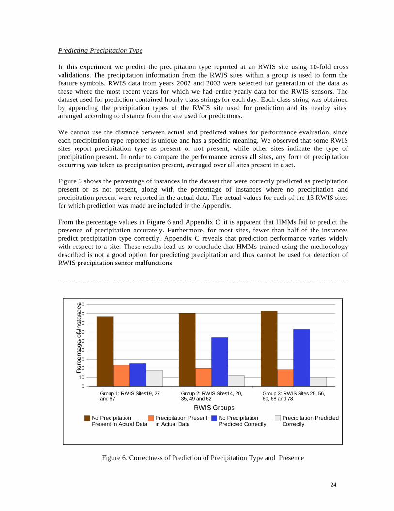
Figure 6 shows the percentage of instances in the dataset that were correctly predicted as precipitation
present or as not present, along with the percentage of instances where no precipitation and
precipitation present were reported in the actual data. The actual values for each of the 13 RWIS sites
for which prediction was made are included in the Appendix.
From the percentage values in Figure 6 and Appendix C, it is apparent that HMMs fail to predict the
presence of precipitation accurately. Furthermore, for most sites, fewer than half of the instances
predict precipitation type correctly. Appendix C reveals that prediction performance varies widely
with respect to a site. These results lead us to conclude that HMMs trained using the methodology
described is not a good option for predicting precipitation and thus cannot be used for detection of
RWIS precipitation sensor malfunctions.
--------------------------------------------------------------------------------------------------------------------------
Group 1: RWIS Sites19, 27 and 67
Group 2: RWIS Sites14, 20, 35, 49 and 62
Group 3: RWIS Sites 25, 56, 60, 68 and 78
0
10
20
30
40
50
60
70
80
90
No Precipitation Present in Actual Data
Precipitation Present in Actual Data
No Precipitation Predicted Correctly
Precipitation Predicted Correctly
RWIS Groups
Pe
rce
nta
ge
of
Insta
nce
s
Figure 6. Correctness of Prediction of Precipitation Type and Presence
25
Conclusion
Hidden Markov Models performed well for classifying discretized temperature values but failed to
predict precipitation type correctly in most cases. A threshold distance of 3 between the actual and the
predicted temperature class value may be used to detect temperature sensor malfunctions. When
predicting temperature, a single model of a group obtained from using the combined dataset yielded
results similar to those obtained from predicting temperature at single sites over a group. This leads us
to conclude that a single model built using datasets of all sites together can be effectively used to
identity malfunctions at any site in the group. We find the models produced by HMM for
precipitation type have a high error when classifying the presence or absence of precipitation and
should not be used for precipitation predictions. However, as concluded in Phase I of this project, a
combination of the machine learning methods J48 and Bayes Nets can be used to detect precipitation
sensor malfunctions, with J48 being used to predict the absence of precipitation and Bayesian
networks, the presence of precipitation.
References
[1] Crouch, C.,Crouch, D., Maclin, R. and Polumeetal, A. Automatic Detection of RWIS Sensor
Malfunction (Phase I), Final Report, NATSRL, University of Minnesota, Duluth, MN, 2007.
[2] Rabiner, L. and Juang, B., An Introduction to Hidden Markov Models, IEEE ASSP Magazine, pp.
4-15 , January 1986.
[3] Baum, L. and Petrie, T., Statistical inference for probabilistic functions of finite state markov
chains, Annals of Mathematical Statistics, vol. 37, 1966.
[4] Viterbi, A., Error bounds for convolutional codes and asymptotically optimum decoding
algorithm, IEEE Transactions on Information Theory, vol. IT-13, no. 2, pp. 260–269, April 1967.
[5] Forney, J., The Viterbi algorithm, Proceedings of the IEEE, vol. 61, no. 3, pp. 268–278, March
1973
[6] Dunham, M. Data Mining: Introductory and Advanced Topics, Prentice Hall, 2003.
[7] Durbin, R., Eddy, S., Krogh, A. and Mitchison, G., Biological Sequence Analysis: Probabilistic
models of proteins and nucleic acids, Cambridge University Press, 1998
[8] National Climatic Data Center, Data Documentation for Data Set 3282 (DSI-3282): ASOS Surface Airways Hourly Observations, National Climatic Data Center, Asheville, NC, May 2005.
[9] Quinlan, R., Induction of Decision Trees, Machine Learning, vol. 1, pp. 81-106, 1986.
[10] Dougherty, J., Kohavi, R. and Sahami, M., Supervised and unsupervised discretization of
continuous features, Proceedings of the Twelfth International Conference on Machine Learning,
pp 94-202, 1995.
[11] Witten, I. and Frank, E., Data Mining: Practical machine learning tools and techniques, 2nd Edition, Morgan Kaufmann, San Francisco, 2005.
[12] Murphy, K., Hidden Markov Model (HMM) Toolbox for MATLAB, 1998, www.cs.ubc.ca/~murphyk/
Software/HMM/hmm.html.

26
APPENDIX
Experimental Results
27
Set 1 Set 2
19 27 67 14 20 35 49 62
Distance 0 18.48% 16.18% 19.30% 21.94% 27.37% 22.86% 18.55% 22.37%
1 68.31% 28.67% 67.63% 73.11% 59.03% 65.06% 60.16% 70.88%
2 12.08% 49.85% 12.19% 4.83% 12.24% 11.09% 16.17% 4.38%
3 1.09% 4.59% 0.88% 0.11% 1.32% 0.95% 3.57% 1.15%
4 0.04% 0.71% 0.00% 0.00% 0.04% 0.04% 1.12% 0.53%
5 0.00% 0.01% 0.00% 0.00% 0.00% 0.00% 0.35% 0.67%
6 0.00% 0.00% 0.00% 0.00% 0.00% 0.00% 0.08% 0.00%
7 0.00% 0.00% 0.00% 0.00% 0.00% 0.00% 0.00% 0.00%
8 0.00% 0.00% 0.00% 0.00% 0.00% 0.00% 0.00% 0.01%
Set 3
25 56 60 68 78
Distance 0 42.65% 44.42% 39.60% 20.11% 39.69%
1 52.82% 49.00% 53.09% 27.20% 39.26%
2 4.33% 6.14% 6.96% 18.24% 16.86%
3 0.20% 0.42% 0.35% 8.36% 1.99%
4 0.01% 0.02% 0.00% 14.59% 0.51%
5 0.00% 0.00% 0.00% 7.17% 1.20%
6 0.00% 0.00% 0.00% 3.83% 0.49%
7 0.00% 0.00% 0.00% 0.46% 0.00%
8 0.00% 0.00% 0.00% 0.02% 0.00%
Percentage of instances with a certain distance between the actual and predicted temperature class value,
obtained by using HMM to predict temperature class

28
0.00%
10.00%
20.00%
30.00%
40.00%
50.00%
60.00%
70.00%
80.00%
0 1 2 3 4 5 6 7 8
Distance |actual-predicted|
Perc
enta
ge o
f In
sta
nces
19 27 67 14 20 35 49 62 25 56 60 68 78
Percentage of instances with a certain distance between the actual and predicted temperature class value,
obtained by using HMM to predict temperature class
29
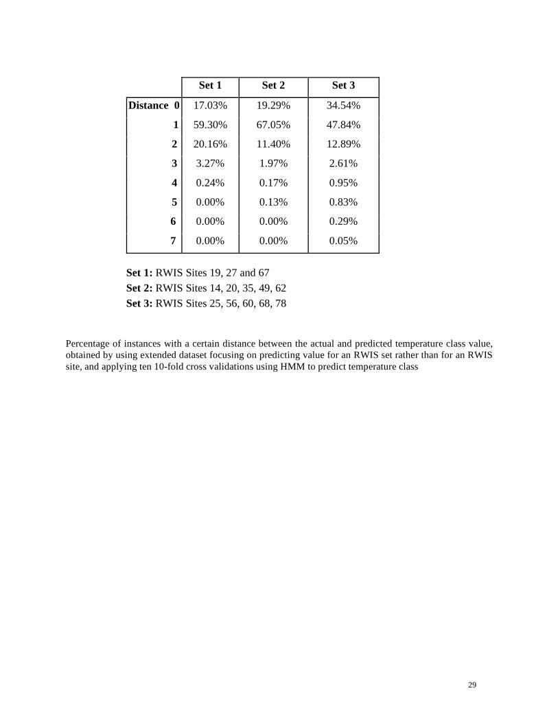
Set 1 Set 2 Set 3
Distance 0 17.03% 19.29% 34.54%
1 59.30% 67.05% 47.84%
2 20.16% 11.40% 12.89%
3 3.27% 1.97% 2.61%
4 0.24% 0.17% 0.95%
5 0.00% 0.13% 0.83%
6 0.00% 0.00% 0.29%
7 0.00% 0.00% 0.05%
Set 1: RWIS Sites 19, 27 and 67
Set 2: RWIS Sites 14, 20, 35, 49, 62
Set 3: RWIS Sites 25, 56, 60, 68, 78
Percentage of instances with a certain distance between the actual and predicted temperature class value,
obtained by using extended dataset focusing on predicting value for an RWIS set rather than for an RWIS
site, and applying ten 10-fold cross validations using HMM to predict temperature class
30
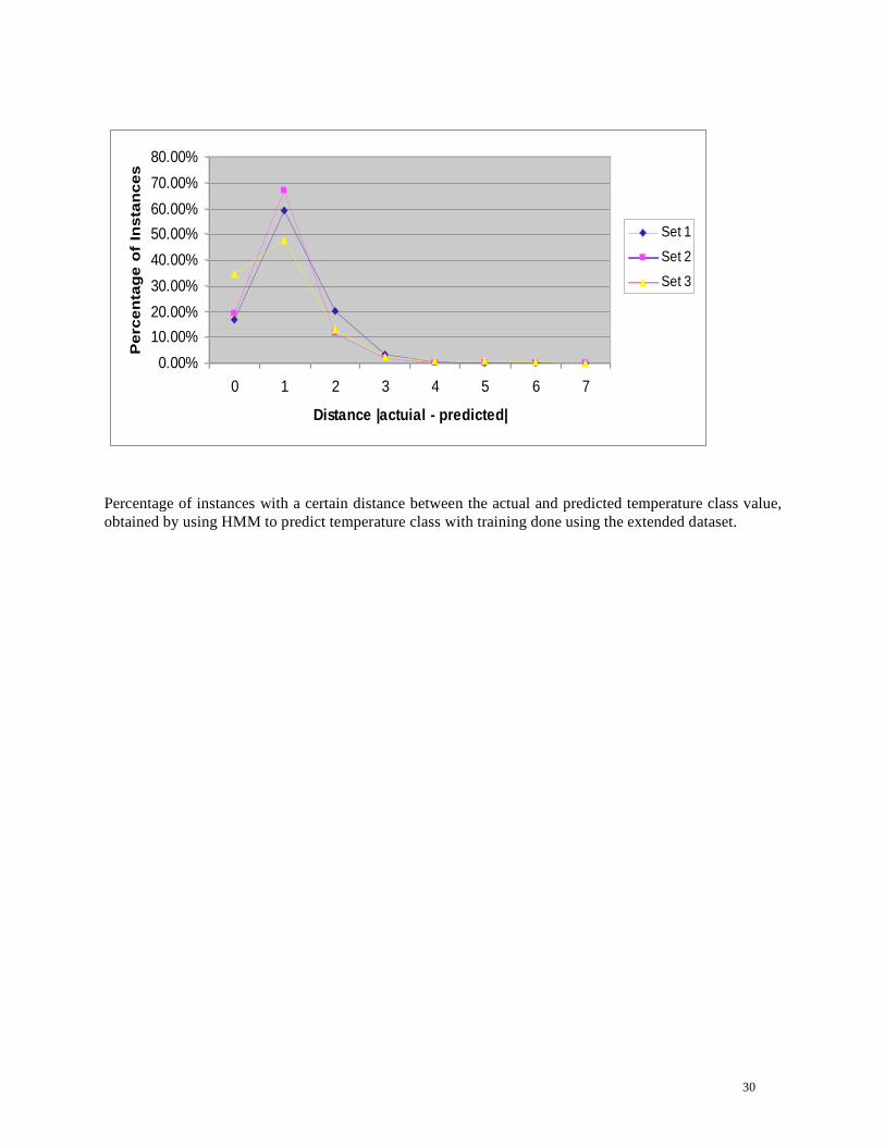
0.00%
10.00%
20.00%
30.00%
40.00%
50.00%
60.00%
70.00%
80.00%
0 1 2 3 4 5 6 7
Distance |actuial - predicted|
Pe
rce
nta
ge
of
Ins
tan
ce
s
Set 1
Set 2
Set 3
Percentage of instances with a certain distance between the actual and predicted temperature class value,
obtained by using HMM to predict temperature class with training done using the extended dataset.

31
RWIS
Site
% of instance
with no
precipitation
reported in data
% of instance
with
precipitation
reported in
data
% of instances
where no
precipitation is
predicted
correctly
% of instances
where
precipitation is
predicted correctly
Set 1 19 85.71 14.28 55.22 4.79
27 77.23 22.77 13.33 18.72
67 67.3 32.69 5.36 28.35
Set 2 14 74.61 24.38 27.22 18.08
20 72.74 27.25 16.96 21.43
35 83.58 16.41 71.19 6.85
49 84.66 15.33 71.24 7.34
Set 3 62 85.82 14.17 80.8 6.38
25 83.1 16.9 73.4 7.7
56 85.25 14.74 74.25 4.27
60 78 20 53.64 9.39
68 86.41 13.59 73.69 5.15
78 83.89 16.11 55.91 7.73
Results obtained from predicting precipitation type using HMM.

32