Automated suitable drainage network extraction from digital

HYDROLOGICAL PROCESSESHydrol. Process. (in press)Published online in Wiley InterScience (www.interscience.wiley.com). DOI: 10.1002/hyp.5911

Automated suitable drainage network extraction fromdigital elevation models in Taiwan’s upstream watersheds

Wen-Tzu Lin,1 Wen-Chieh Chou,2* Chao-Yuan Lin,3 Pi-Hui Huang4 and Jing-Shyan Tsai5

1 Institute of Environmental Planning and Design, Ming Dao University, Changhua County 523, Taiwan2 Department of Civil Engineering and Engineering Informatics, Chung Hua University, Hsinchu City 300, Taiwan

3 Department of Soil and Water Conservation, National Chung Hsing University, Taichung City 402, Taiwan4 Graduate Institute of Civil and Hydraulic Engineering, Feng Chia University, Taichung City 407, Taiwan

5 Department of Landscape Architecture, Chung Hua University, Hsinchu City 300, Taiwan

Abstract:

Automatically extracting drainage networks from digital elevation models coupled with the constant stream thresholdvalue is a regular method. These extracted networks can be verified by comparing the channel initiation points withthose from real networks. From the results analysed, the differences in channel initiation points will affect the networkgeometries, geomorphological indices and hydrological responses. This paper develops two automatic algorithms, theheadwater-tracing method and the fitness index, to trace the flow paths from headwaters to the outlet and to calculatethe reasonable stream threshold. Instead of the method determined by trial and error or field survey, the accuratechannel initiation points can be obtained from airborne photographs coupled with high-resolution SPOT images forsuitable drainage network extraction. Copyright 2005 John Wiley & Sons, Ltd.

KEY WORDS channel initiation; headwater-tracing method; fitness index; stream network; geomorphological indices;hydrological responses

INTRODUCTION

A digital terrain model (DTM) is an ordered array of numbers that represents the spatial distribution of terraincharacteristics (Doyle, 1978). When there is only one property, elevation, the term digital elevation model(DEM) is used (Collins and Moon, 1981). Demel et al. (1982) categorized DEMs as regular grids, digitalcontours and triangulated irregular networks according to their data structure. In spite of the fact that DEMsin the form of triangular irregular networks or digital contour lines seem to be more adequate for representingterrain morphology (Palacios-Velez and Cuevas-Renaud, 1986; Moore et al., 1991), regular-grid DEMs havebeen adopted more often for network extraction (Peucker and Douglas, 1975; Mark, 1984; O’Callaghan andMark, 1984; Jenson, 1985; Band, 1986, 1989; Jenson and Domingue, 1988; Fairfield and Leymarie, 1991;Tarboton et al., 1991; Tribe, 1992). The regular grid is the most popular DEM for terrain because of its simpleand ordered data characteristics. It can be used to derive a wealth of information about the morphology of aland surface (US Geological Survey, 1987).

A variety of methods have been developed to process raster DEMs automatically to extract drainagenetworks and measure their properties (O’Callaghan and Mark, 1984; Band, 1986; Jenson and Domingue,1988; Tarboton et al., 1991; Martz and Garbrecht, 1992, 1998, 1999). The most commonly used proceduresfor extracting drainage networks from raster DEMs are based on O’Callaghan and Mark’s (1984) algorithmfor flow direction determination, coupled with an arbitrary constant value for the minimum contributingarea needed to form and maintain a channel. The stream threshold Ts choice will influence the extracted

* Correspondence to: Wen-Chieh Chou, Department of Civil Engineering, Chung Hua University, Hsinchu City 300, Taiwan.E-mail: [email protected]

Received 13 February 2003Copyright 2005 John Wiley & Sons, Ltd. Accepted 18 January 2005

W.-T. LIN ET AL.

drainage networks. Generally, Ts is assumed as a constant value, based on personal judgment or visualcomparison of the networks generated with the streamlines identified or digitized from a topographical map(Jenson and Domingue, 1988; Gardner et al., 1991). Other researchers, such as Montgomery and Dietrich(1988), Tarboton et al. (1991) and Dietrich et al. (1993), have devoted themselves to deriving quantitativeapproaches to stream threshold definition according to the link between slope and area power. However,power law relationship studies should be validated further on the influences between the morphology, soiland climate to actual channel initiation. Heretofore, using a constant threshold value to extract drainagenetworks automatically from a DEM is still the most popular method for calculating the geomorphologicaland hydrological information.

With the fast-growing computer technologies and geographic information systems (GISs), a number ofprograms, such as the HYDROLOGY module in ArcView, the DWCON and TERRAIN ANALYSIS modulesin EASI/PACE (Chang, 2002), and TOPAZ (Lacroix et al., 2002), landscape analysis tools were developed toextract drainage networks by combining the Jenson and Domingue (1988) and Garbrecht and Martz (1997)algorithms with GISs. The only way to determine a reasonable stream threshold was trial and error. Trial anderror is not only subjective, but also wastes time when determining the reasonable stream threshold. Channelinitiation information depends on the landform and/or climate characteristics of the watershed. The channelinitiation points, therefore, fluctuate.

The extracted stream network in hydrologic analyses is important because the network indirectly determinesthe hillslope travel distance and network link lengths. The characteristics of the extracted network dependextensively on the definition of channel initiations on the digital landscape. Once the channel initiations aredefined, the essential topology and morphometric characteristics of the corresponding downstream drainagenetwork are implicitly predefined because of their close dependence on channel initiation definition. Thus, theidentification of channel sources is critical for extraction of a representative drainage network from DEMs(ASCE, 1999). This study develops modified algorithms that can easily extract suitable drainage networks,especially using channel initiations. Comparisons between networks extracted from different maps or variousstream thresholds were carried out in quantitative terms by calculating the geomorphological indices and thehydrological responses, represented by the geomorphological instantaneous unit hydrographs (GIUHs) on twoupstream watersheds in central Taiwan.

MATERIALS AND METHODS

Study area

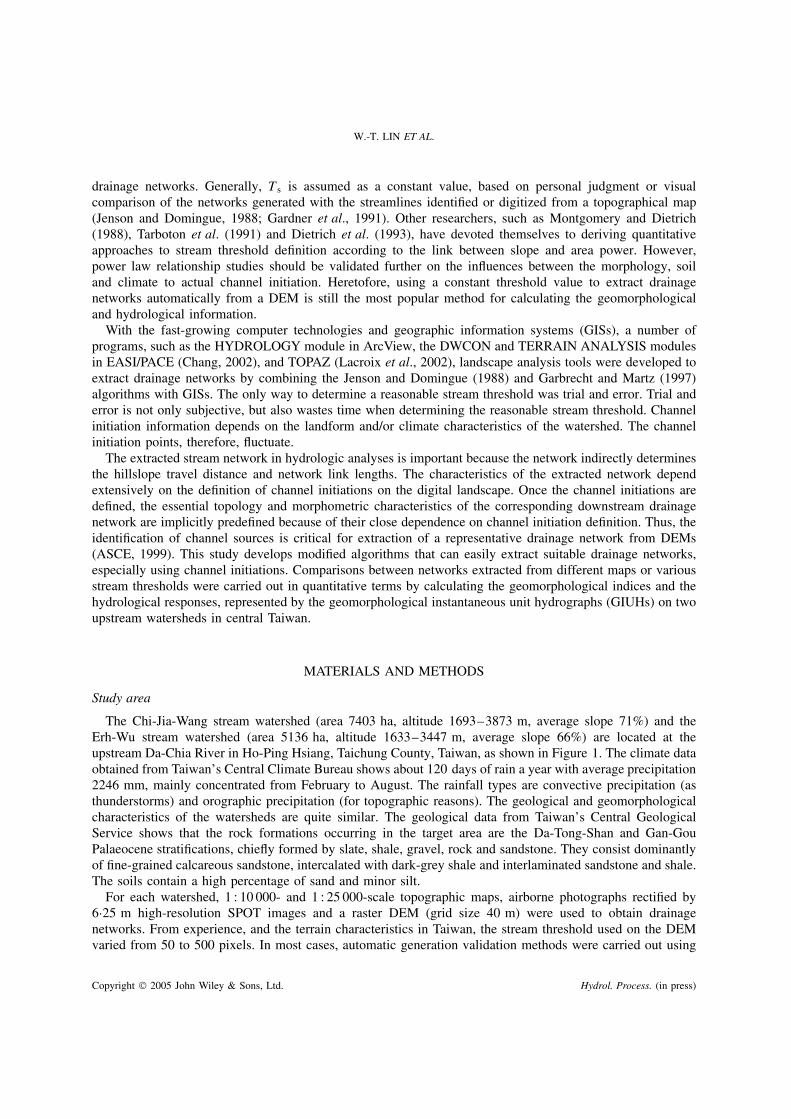
The Chi-Jia-Wang stream watershed (area 7403 ha, altitude 1693–3873 m, average slope 71%) and theErh-Wu stream watershed (area 5136 ha, altitude 1633–3447 m, average slope 66%) are located at theupstream Da-Chia River in Ho-Ping Hsiang, Taichung County, Taiwan, as shown in Figure 1. The climate dataobtained from Taiwan’s Central Climate Bureau shows about 120 days of rain a year with average precipitation2246 mm, mainly concentrated from February to August. The rainfall types are convective precipitation (asthunderstorms) and orographic precipitation (for topographic reasons). The geological and geomorphologicalcharacteristics of the watersheds are quite similar. The geological data from Taiwan’s Central GeologicalService shows that the rock formations occurring in the target area are the Da-Tong-Shan and Gan-GouPalaeocene stratifications, chiefly formed by slate, shale, gravel, rock and sandstone. They consist dominantlyof fine-grained calcareous sandstone, intercalated with dark-grey shale and interlaminated sandstone and shale.The soils contain a high percentage of sand and minor silt.

For each watershed, 1 : 10 000- and 1 : 25 000-scale topographic maps, airborne photographs rectified by6Ð25 m high-resolution SPOT images and a raster DEM (grid size 40 m) were used to obtain drainagenetworks. From experience, and the terrain characteristics in Taiwan, the stream threshold used on the DEMvaried from 50 to 500 pixels. In most cases, automatic generation validation methods were carried out using

Copyright 2005 John Wiley & Sons, Ltd. Hydrol. Process. (in press)

DRAINAGE NETWORK EXTRACTION

drainage networkwatershed boundary

3 60Km

Chi-Jia-Wang streamwatershed

Erh-Wu streamwatershed

Da-Chia

Rive

r

Figure 1. Study area

visual comparison with the blue lines from medium-scale topographic maps or photo-interpretation (Chorowiczet al., 1992). This study selected photo-interpretation to validate the new extraction methods.

Methods

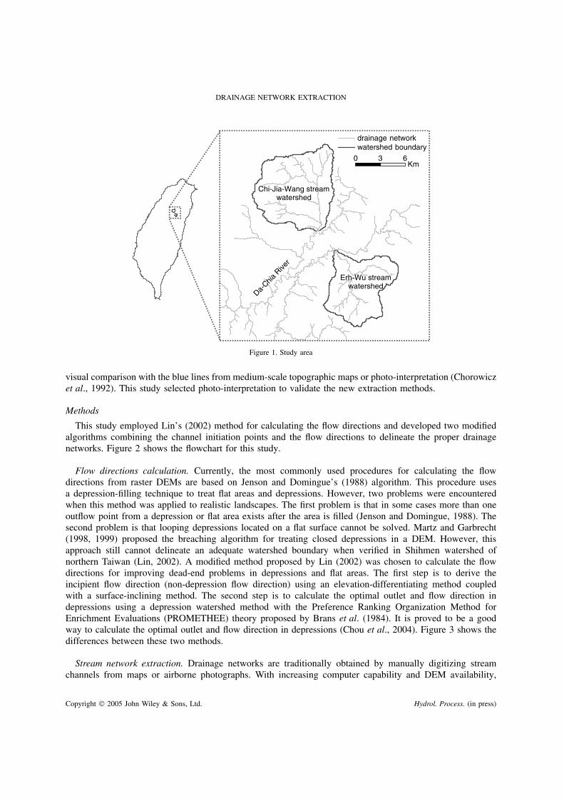
This study employed Lin’s (2002) method for calculating the flow directions and developed two modifiedalgorithms combining the channel initiation points and the flow directions to delineate the proper drainagenetworks. Figure 2 shows the flowchart for this study.

Flow directions calculation. Currently, the most commonly used procedures for calculating the flowdirections from raster DEMs are based on Jenson and Domingue’s (1988) algorithm. This procedure usesa depression-filling technique to treat flat areas and depressions. However, two problems were encounteredwhen this method was applied to realistic landscapes. The first problem is that in some cases more than oneoutflow point from a depression or flat area exists after the area is filled (Jenson and Domingue, 1988). Thesecond problem is that looping depressions located on a flat surface cannot be solved. Martz and Garbrecht(1998, 1999) proposed the breaching algorithm for treating closed depressions in a DEM. However, thisapproach still cannot delineate an adequate watershed boundary when verified in Shihmen watershed ofnorthern Taiwan (Lin, 2002). A modified method proposed by Lin (2002) was chosen to calculate the flowdirections for improving dead-end problems in depressions and flat areas. The first step is to derive theincipient flow direction (non-depression flow direction) using an elevation-differentiating method coupledwith a surface-inclining method. The second step is to calculate the optimal outlet and flow direction indepressions using a depression watershed method with the Preference Ranking Organization Method forEnrichment Evaluations (PROMETHEE) theory proposed by Brans et al. (1984). It is proved to be a goodway to calculate the optimal outlet and flow direction in depressions (Chou et al., 2004). Figure 3 shows thedifferences between these two methods.

Stream network extraction. Drainage networks are traditionally obtained by manually digitizing streamchannels from maps or airborne photographs. With increasing computer capability and DEM availability,


W.-T. LIN ET AL.

results and discussion

data collection

flow direction calculation

digital elevation model1. topographical maps2. airborne photos3. SPOT satellite image

1. fitness index2. headwaters-tracing method3. constant stream threshold

drainage networks

Geomorphological indices hydrological response

WinG

rid system

Figure 2. Flowchart of this study

clipping DEM

filling depression in a DEM

computing depressionlessflow direction

computing non-depression flow direction

seeking depression watershed

computing the outlet of depressionwatershed using PROMETHEE

computing depression flow direction

computing the flow accumulation

delineating watershed extracting drainage network

assigned a constant threshold

Lin’s method

Jenson and Dom

ingue’s method

Figure 3. Differences in extracting a drainage network between the Jenson and Domingue and the Lin methods

attempts have been made to extract networks from DEMs via computer programs. The ‘constant-threshold’method was used to calculate the number of upstream elements, i.e. the number of cells that contribute surfaceflow to any particular cell. Cells with catchment numbers greater than a given threshold are considered onthe flow path. The smaller the chosen threshold, the more complicated are the channels obtained. Tribe



(1991) pointed out a problem involved in positioning the drainage network end that would prevent successfuldelineation of fully connected drainage networks. Positioning of the ends of drainage networks fluctuates withthe threshold value.

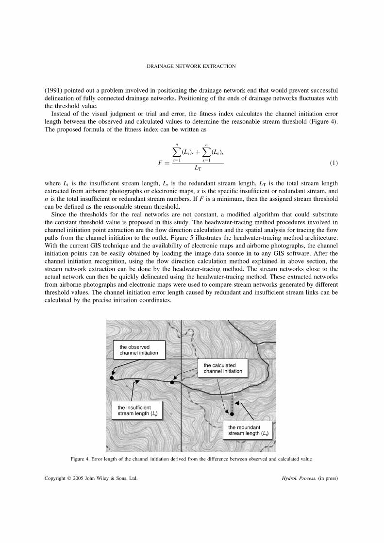
Instead of the visual judgment or trial and error, the fitness index calculates the channel initiation errorlength between the observed and calculated values to determine the reasonable stream threshold (Figure 4).The proposed formula of the fitness index can be written as

F D

n∑sD1

�Li�s Cn∑

sD1

�Lr�s

LT�1�

where Li is the insufficient stream length, Lr is the redundant stream length, LT is the total stream lengthextracted from airborne photographs or electronic maps, s is the specific insufficient or redundant stream, andn is the total insufficient or redundant stream numbers. If F is a minimum, then the assigned stream thresholdcan be defined as the reasonable stream threshold.

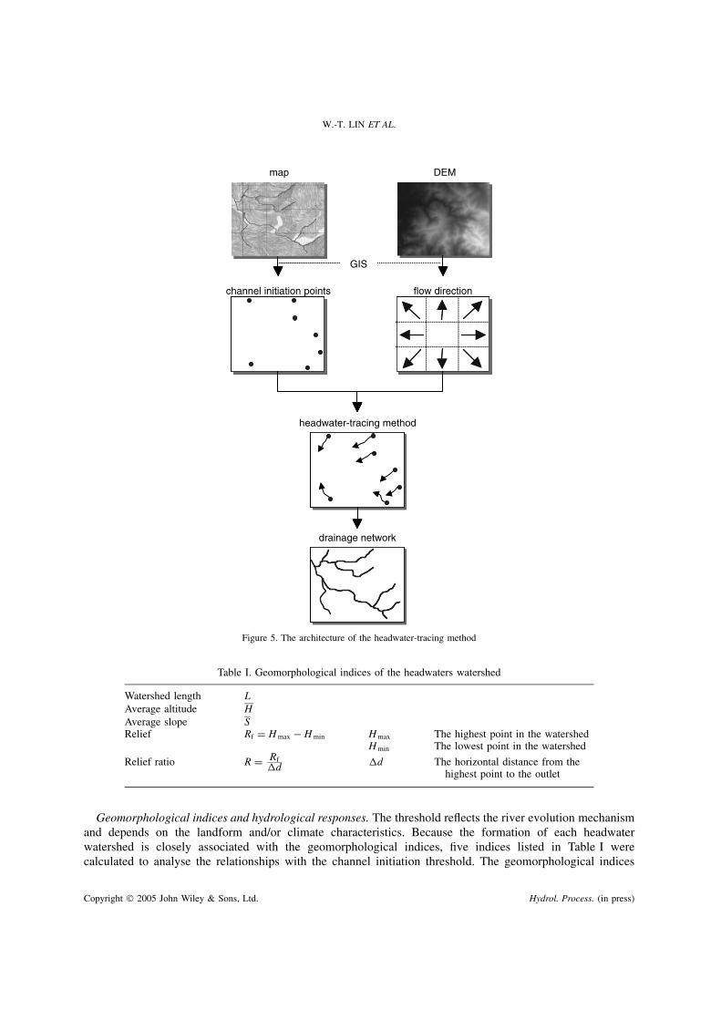
Since the thresholds for the real networks are not constant, a modified algorithm that could substitutethe constant threshold value is proposed in this study. The headwater-tracing method procedures involved inchannel initiation point extraction are the flow direction calculation and the spatial analysis for tracing the flowpaths from the channel initiation to the outlet. Figure 5 illustrates the headwater-tracing method architecture.With the current GIS technique and the availability of electronic maps and airborne photographs, the channelinitiation points can be easily obtained by loading the image data source in to any GIS software. After thechannel initiation recognition, using the flow direction calculation method explained in above section, thestream network extraction can be done by the headwater-tracing method. The stream networks close to theactual network can then be quickly delineated using the headwater-tracing method. These extracted networksfrom airborne photographs and electronic maps were used to compare stream networks generated by differentthreshold values. The channel initiation error length caused by redundant and insufficient stream links can becalculated by the precise initiation coordinates.

the insufficientstream length (Li)

the redundantstream length (Lr)

the calculatedchannel initiation

the observedchannel initiation

Figure 4. Error length of the channel initiation derived from the difference between observed and calculated value


W.-T. LIN ET AL.

map DEM

channel initiation points flow direction

headwater-tracing method

drainage network

GIS

Figure 5. The architecture of the headwater-tracing method

Table I. Geomorphological indices of the headwaters watershed

Watershed length LAverage altitude HAverage slope SRelief Rf D Hmax � Hmin Hmax The highest point in the watershed

Hmin The lowest point in the watershed

Relief ratio R D Rfd d The horizontal distance from the

highest point to the outlet

Geomorphological indices and hydrological responses. The threshold reflects the river evolution mechanismand depends on the landform and/or climate characteristics. Because the formation of each headwaterwatershed is closely associated with the geomorphological indices, five indices listed in Table I werecalculated to analyse the relationships with the channel initiation threshold. The geomorphological indices



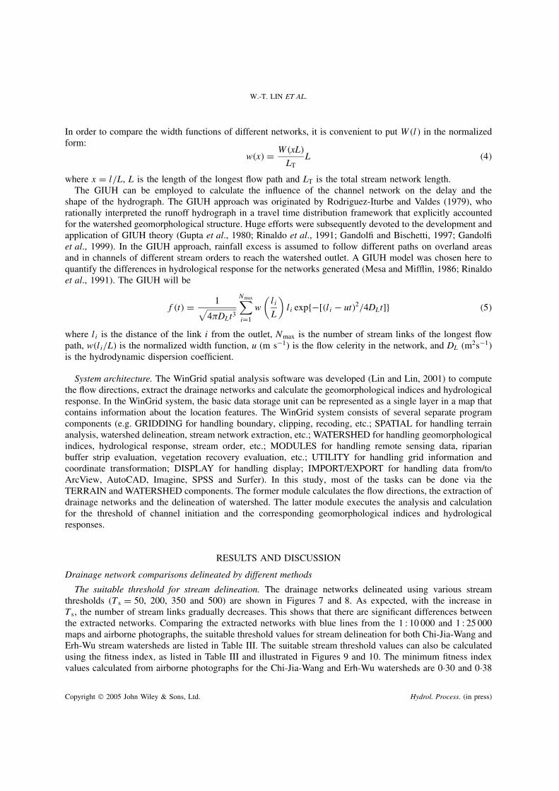
Table II. Geomorphological indices of the drainage network

Number of headwaters Nh The inlet numbers of first-order streamNumber of stream links NMain stream length (m) L0

Total stream length (m) LT Dn∑i

Li The total length of stream within awatershed. Li: stream link length

Catchment order (unitless) � A number that designates the relative positionof stream segment in a drainage network

Drainage density (m�1) Ds D LTA A: watershed area

Drainage frequency (m�2) Fs D NwA The number of stream segments per unit area

of the drainage network (Table II) were also calculated to compare the networks delineated using variousmethods.

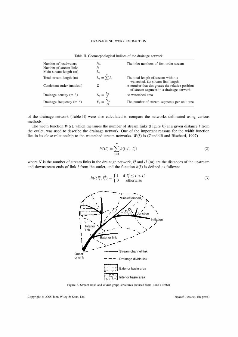
The width function W�l�, which measures the number of stream links (Figure 6) at a given distance l fromthe outlet, was used to describe the drainage network. One of the important reasons for the width functionlies in its close relationship to the watershed stream networks. W�l� is (Gandolfi and Bischetti, 1997)

W�l� DN∑

iD1

b�l; lui , ld

i � �2�

where N is the number of stream links in the drainage network, lui and ld

i (m) are the distances of the upstreamand downstream ends of link i from the outlet, and the function b�l� is defined as follows:

b�l; lui , ld

i � D{

1 if ldi � l < lu

i0 otherwise

�3�

Stream channel link

Drainage divide link

Exterior basin area

Interior basin area

Initiation

Junction

Exterior link

Interiorlink

Outletor sink

Subwatershed

Figure 6. Stream links and divide graph structures (revised from Band (1986))


W.-T. LIN ET AL.

In order to compare the width functions of different networks, it is convenient to put W�l� in the normalizedform:

w�x� D W�xL�

LTL �4�

where x D l/L, L is the length of the longest flow path and LT is the total stream network length.The GIUH can be employed to calculate the influence of the channel network on the delay and the

shape of the hydrograph. The GIUH approach was originated by Rodriguez-Iturbe and Valdes (1979), whorationally interpreted the runoff hydrograph in a travel time distribution framework that explicitly accountedfor the watershed geomorphological structure. Huge efforts were subsequently devoted to the development andapplication of GIUH theory (Gupta et al., 1980; Rinaldo et al., 1991; Gandolfi and Bischetti, 1997; Gandolfiet al., 1999). In the GIUH approach, rainfall excess is assumed to follow different paths on overland areasand in channels of different stream orders to reach the watershed outlet. A GIUH model was chosen here toquantify the differences in hydrological response for the networks generated (Mesa and Mifflin, 1986; Rinaldoet al., 1991). The GIUH will be

f�t� D 1√4�DLt3

Nmax∑iD1

w

(li

L

)li expf�[�li � ut�2/4DLt]g �5�

where li is the distance of the link i from the outlet, Nmax is the number of stream links of the longest flowpath, w�li/L� is the normalized width function, u (m s�1) is the flow celerity in the network, and DL (m2s�1)is the hydrodynamic dispersion coefficient.

System architecture. The WinGrid spatial analysis software was developed (Lin and Lin, 2001) to computethe flow directions, extract the drainage networks and calculate the geomorphological indices and hydrologicalresponse. In the WinGrid system, the basic data storage unit can be represented as a single layer in a map thatcontains information about the location features. The WinGrid system consists of several separate programcomponents (e.g. GRIDDING for handling boundary, clipping, recoding, etc.; SPATIAL for handling terrainanalysis, watershed delineation, stream network extraction, etc.; WATERSHED for handling geomorphologicalindices, hydrological response, stream order, etc.; MODULES for handling remote sensing data, riparianbuffer strip evaluation, vegetation recovery evaluation, etc.; UTILITY for handling grid information andcoordinate transformation; DISPLAY for handling display; IMPORT/EXPORT for handling data from/toArcView, AutoCAD, Imagine, SPSS and Surfer). In this study, most of the tasks can be done via theTERRAIN and WATERSHED components. The former module calculates the flow directions, the extraction ofdrainage networks and the delineation of watershed. The latter module executes the analysis and calculationfor the threshold of channel initiation and the corresponding geomorphological indices and hydrologicalresponses.

RESULTS AND DISCUSSION

Drainage network comparisons delineated by different methods

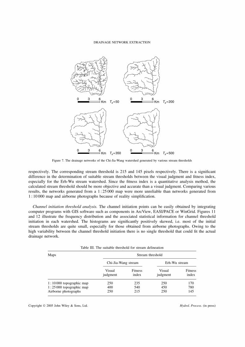
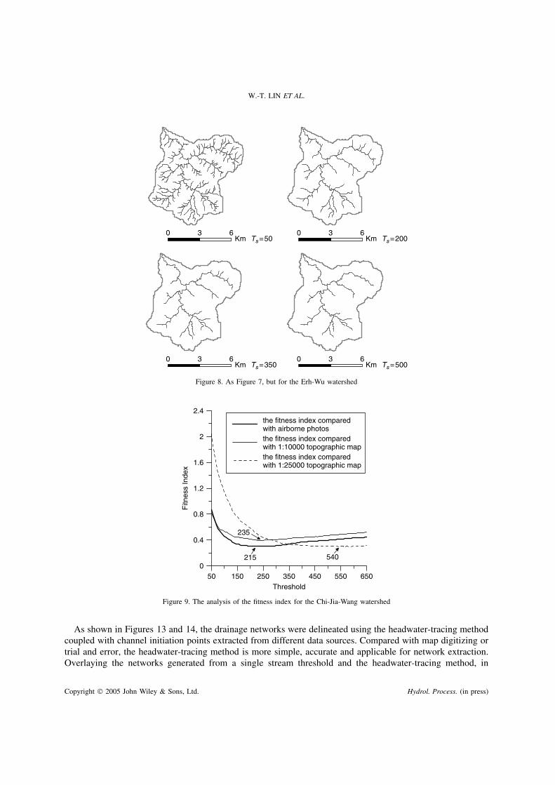
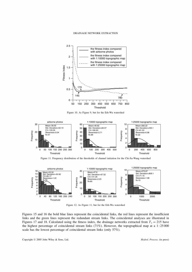
The suitable threshold for stream delineation. The drainage networks delineated using various streamthresholds (Ts D 50, 200, 350 and 500) are shown in Figures 7 and 8. As expected, with the increase inTs, the number of stream links gradually decreases. This shows that there are significant differences betweenthe extracted networks. Comparing the extracted networks with blue lines from the 1 : 10 000 and 1 : 25 000maps and airborne photographs, the suitable threshold values for stream delineation for both Chi-Jia-Wang andErh-Wu stream watersheds are listed in Table III. The suitable stream threshold values can also be calculatedusing the fitness index, as listed in Table III and illustrated in Figures 9 and 10. The minimum fitness indexvalues calculated from airborne photographs for the Chi-Jia-Wang and Erh-Wu watersheds are 0Ð30 and 0Ð38



Ts =500 3

Km6

Ts =3500 3

Km6

Ts =5000 3

Km6

Ts =2000 3

Km6

Figure 7. The drainage networks of the Chi-Jia-Wang watershed generated by various stream thresholds

respectively. The corresponding stream threshold is 215 and 145 pixels respectively. There is a significantdifference in the determination of suitable stream thresholds between the visual judgment and fitness index,especially for the Erh-Wu stream watershed. Since the fitness index is a quantitative analysis method, thecalculated stream threshold should be more objective and accurate than a visual judgment. Comparing variousresults, the networks generated from a 1 : 25 000 map were more unreliable than networks generated from1 : 10 000 map and airborne photographs because of reality simplification.

Channel initiation threshold analysis. The channel initiation points can be easily obtained by integratingcomputer programs with GIS software such as components in ArcView, EASI/PACE or WinGrid. Figures 11and 12 illustrate the frequency distribution and the associated statistical information for channel thresholdinitiation in each watershed. The histograms are significantly positively skewed, i.e. most of the initialstream thresholds are quite small, especially for those obtained from airborne photographs. Owing to thehigh variability between the channel threshold initiation there is no single threshold that could fit the actualdrainage network.

Table III. The suitable threshold for stream delineation

Maps Stream threshold

Chi-Jia-Wang stream Erh-Wu stream

Visualjudgment

Fitnessindex

Visualjudgment

Fitnessindex

1 : 10 000 topographic map 250 235 250 1701 : 25 000 topographic map 400 540 450 780Airborne photographs 250 215 250 145


W.-T. LIN ET AL.

0 3 6Km Ts =50

0 3 6Km Ts =350

0 3 6Km Ts =500

0 3 6Km Ts =200

Figure 8. As Figure 7, but for the Erh-Wu watershed

50 150 250 350 450 550 650Threshold

0

0.4

0.8

1.2

1.6

2

2.4

Fitn

ess

Inde

x

the fitness index comparedwith airborne photosthe fitness index comparedwith 1:10000 topographic mapthe fitness index comparedwith 1:25000 topographic map

215

235

540

Figure 9. The analysis of the fitness index for the Chi-Jia-Wang watershed

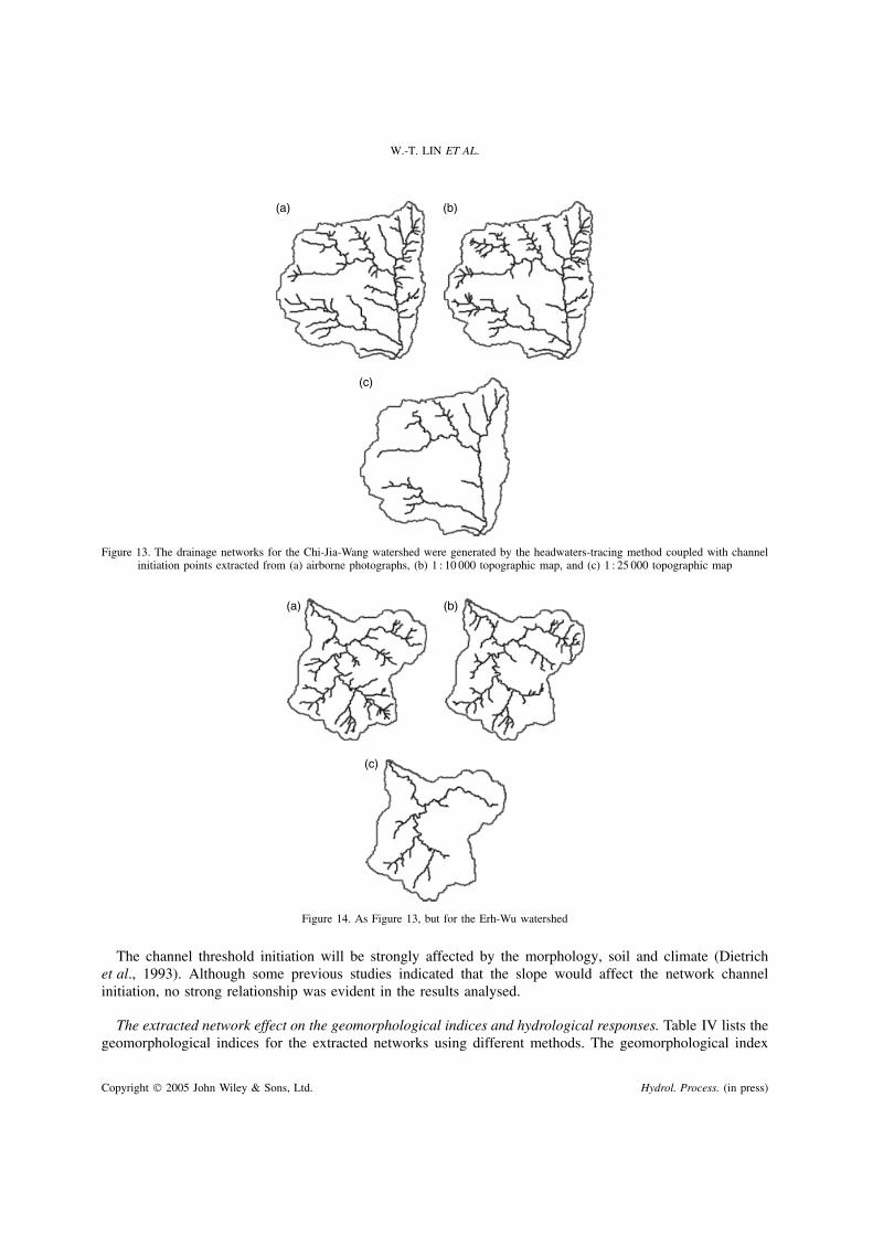
As shown in Figures 13 and 14, the drainage networks were delineated using the headwater-tracing methodcoupled with channel initiation points extracted from different data sources. Compared with map digitizing ortrial and error, the headwater-tracing method is more simple, accurate and applicable for network extraction.Overlaying the networks generated from a single stream threshold and the headwater-tracing method, in



50 150 250 350 450 550 650 750 850

Threshold

0

0.5

1

1.5

2

2.5

Fitn

ess

Inde

x

the fitness index comparedwith airborne photos

the fitness index comparedwith 1:10000 topographic map

the fitness index comparedwith 1:25000 topographic map

145

170

780


Threshold

300250200150100500

Threshold

5004003002001000

airborne photos

Fre

quen

cy

30

20

10

0

Mean=39.00Std. Deviation=52.10CV=133.59Skewness=3.04N=57

1:10000 topographic map

Fre

quen

cy

60

50

40

30

20

10

0


Threshold

8006004002000

1:25000 topographic mapF

requ

ency

10

8

6

4

2

0


Figure 11. Frequency distribution of the thresholds of channel initiation for the Chi-Jia-Wang watershed

Threshold

24020016012080400

airborne photos

Fre

quen

cy

1614121086420


Threshold

300250200150100500


Fre

quen

cy

40

30

20

10

0


Threshold

200010000


Fre

quen

cy

10

8

6

4

2

0



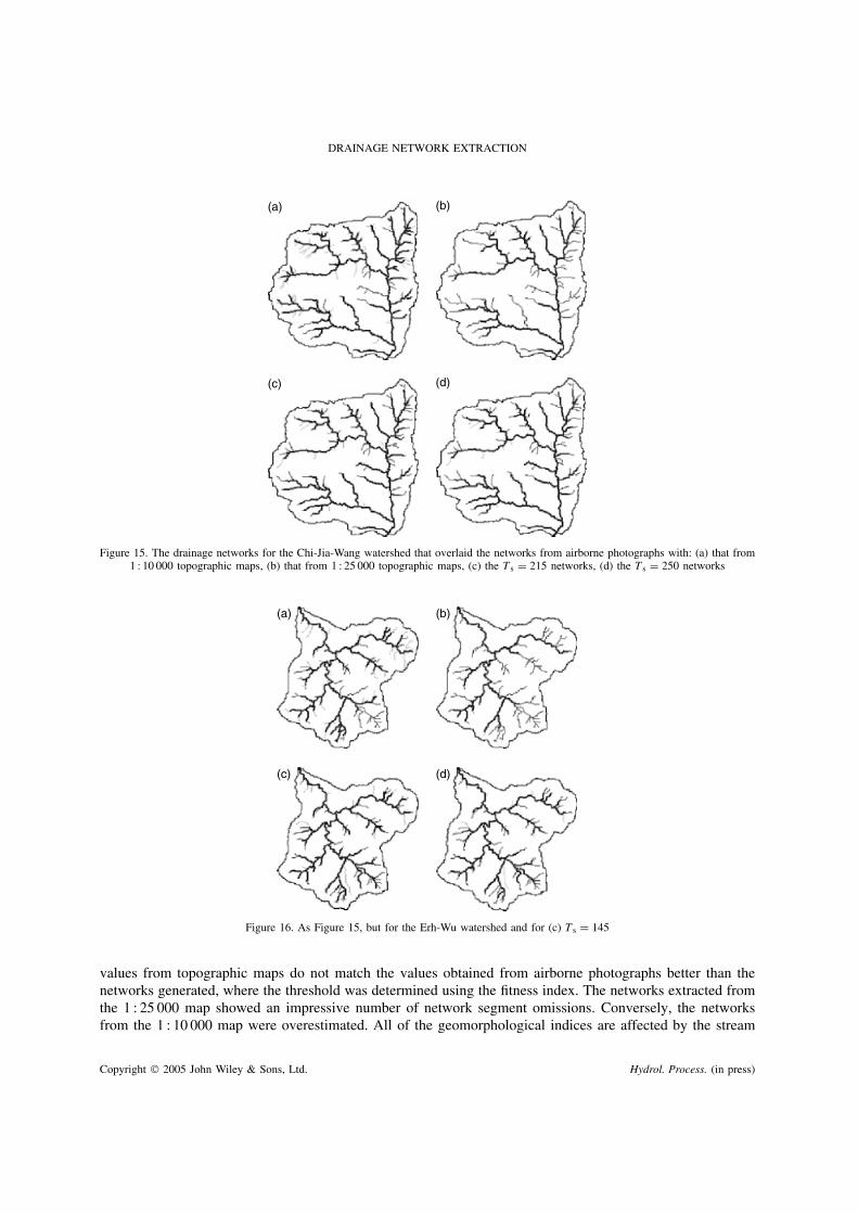
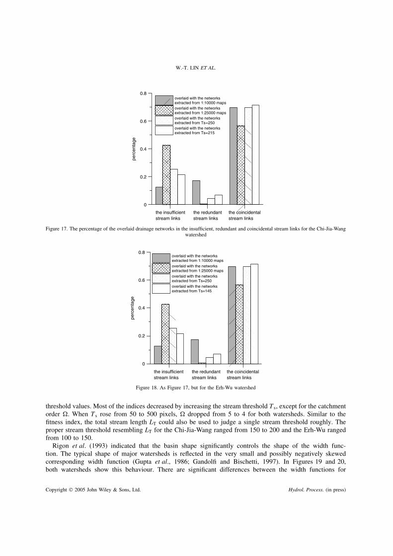
Figures 15 and 16 the bold blue lines represent the coincidental links, the red lines represent the insufficientlinks and the green lines represent the redundant stream links. The coincidental analyses are illustrated inFigures 17 and 18. Calculated using the fitness index, the drainage networks extracted from Ts D 215 havethe highest percentage of coincidental stream links (71%). However, the topographical map at a 1 : 25 000scale has the lowest percentage of coincidental stream links (only 57%).


W.-T. LIN ET AL.

(a)

(c)

(b)

Figure 13. The drainage networks for the Chi-Jia-Wang watershed were generated by the headwaters-tracing method coupled with channelinitiation points extracted from (a) airborne photographs, (b) 1 : 10 000 topographic map, and (c) 1 : 25 000 topographic map

(a)

(c)

(b)


The channel threshold initiation will be strongly affected by the morphology, soil and climate (Dietrichet al., 1993). Although some previous studies indicated that the slope would affect the network channelinitiation, no strong relationship was evident in the results analysed.

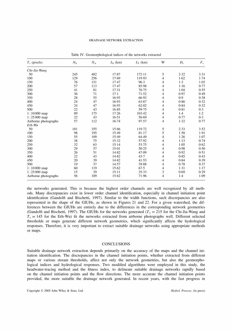
The extracted network effect on the geomorphological indices and hydrological responses. Table IV lists thegeomorphological indices for the extracted networks using different methods. The geomorphological index



(a) (b)

(c) (d)

Figure 15. The drainage networks for the Chi-Jia-Wang watershed that overlaid the networks from airborne photographs with: (a) that from1 : 10 000 topographic maps, (b) that from 1 : 25 000 topographic maps, (c) the Ts D 215 networks, (d) the Ts D 250 networks

(a) (b)

(c) (d)

Figure 16. As Figure 15, but for the Erh-Wu watershed and for (c) Ts D 145

values from topographic maps do not match the values obtained from airborne photographs better than thenetworks generated, where the threshold was determined using the fitness index. The networks extracted fromthe 1 : 25 000 map showed an impressive number of network segment omissions. Conversely, the networksfrom the 1 : 10 000 map were overestimated. All of the geomorphological indices are affected by the stream


W.-T. LIN ET AL.

0

0.2

0.4

0.6

0.8

perc

enta

ge

overlaid with the networksextracted from 1:10000 mapsoverlaid with the networksextracted from 1:25000 mapsoverlaid with the networksextracted from Ts=250overlaid with the networksextracted from Ts=215

the insufficientstream links

the redundantstream links

the coincidentalstream links

Figure 17. The percentage of the overlaid drainage networks in the insufficient, redundant and coincidental stream links for the Chi-Jia-Wangwatershed

0

0.2

0.4

0.6

0.8

perc

enta

ge

overlaid with the networksextracted from 1:10000 maps overlaid with the networksextracted from 1:25000 mapsoverlaid with the networksextracted from Ts=250overlaid with the networksextracted from Ts=145

the insufficientstream links

the redundantstream links

the coincidentalstream links


threshold values. Most of the indices decreased by increasing the stream threshold Ts, except for the catchmentorder �. When Ts rose from 50 to 500 pixels, � dropped from 5 to 4 for both watersheds. Similar to thefitness index, the total stream length LT could also be used to judge a single stream threshold roughly. Theproper stream threshold resembling LT for the Chi-Jia-Wang ranged from 150 to 200 and the Erh-Wu rangedfrom 100 to 150.

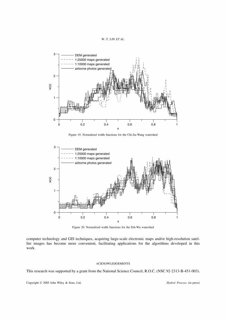
Rigon et al. (1993) indicated that the basin shape significantly controls the shape of the width func-tion. The typical shape of major watersheds is reflected in the very small and possibly negatively skewedcorresponding width function (Gupta et al., 1986; Gandolfi and Bischetti, 1997). In Figures 19 and 20,both watersheds show this behaviour. There are significant differences between the width functions for



Table IV. Geomorphological indices of the networks extracted

Ts (pixels) Nh Nw L0 (km) LT (km) W Ds Fs

Chi-Jia-Wang50 245 482 17Ð87 172Ð11 5 2Ð32 3Ð31

100 129 256 17Ð69 119Ð93 4 1Ð62 1Ð74150 76 151 17Ð47 96Ð3 4 1Ð3 1Ð03200 57 113 17Ð47 85Ð98 4 1Ð16 0Ð77250 41 81 17Ð31 76Ð75 4 1Ð04 0Ð55300 36 71 17Ð1 71Ð52 4 0Ð97 0Ð49350 28 55 16Ð93 66Ð93 4 0Ð9 0Ð38400 24 47 16Ð93 63Ð67 4 0Ð86 0Ð32450 24 47 16Ð93 62Ð02 4 0Ð84 0Ð32500 22 43 16Ð85 59Ð75 4 0Ð81 0Ð31 : 10 000 map 89 175 17Ð26 103Ð42 4 1Ð4 1Ð21 : 25 000 map 22 43 16Ð51 56Ð69 4 0Ð77 0Ð3Airborne photographs 57 112 16Ð74 97Ð57 4 1Ð32 0Ð77Erh-Wu

50 181 355 15Ð66 119Ð72 5 2Ð33 3Ð52100 98 195 15Ð49 81Ð17 5 1Ð58 1Ð91150 55 109 15Ð49 64Ð49 4 1Ð26 1Ð07200 38 75 15Ð32 57Ð92 4 1Ð13 0Ð74250 32 63 15Ð14 53Ð75 4 1Ð05 0Ð62300 29 57 15Ð01 50Ð25 4 0Ð98 0Ð56350 26 51 14Ð82 47Ð09 4 0Ð92 0Ð51400 22 43 14Ð82 43Ð7 4 0Ð85 0Ð43450 20 39 14Ð82 41Ð53 4 0Ð84 0Ð39500 19 37 14Ð57 39Ð88 4 0Ð78 0Ð371 : 10 000 map 60 119 15Ð62 67Ð5 4 1Ð31 1Ð171 : 25 000 map 15 29 15Ð11 35Ð33 3 0Ð69 0Ð29Airborne photographs 56 109 15Ð62 71Ð96 4 1Ð4 1Ð09

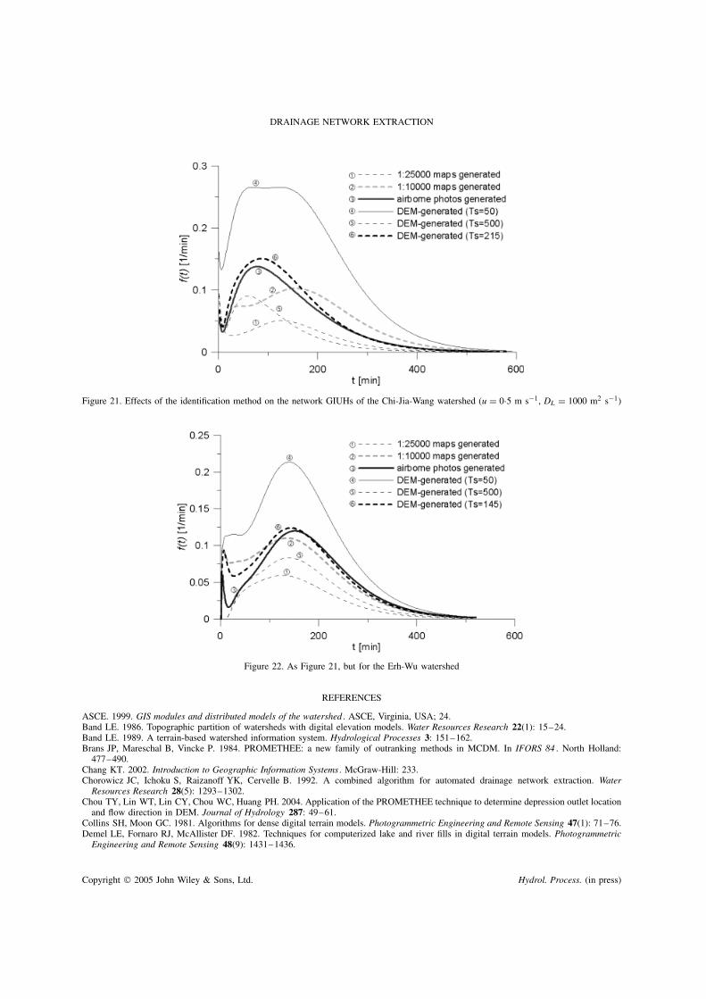
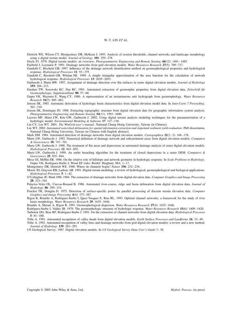
the networks generated. This is because the highest order channels are well recognized by all meth-ods. Many discrepancies exist in lower order channel identification, especially in channel initiation pointidentification (Gandolfi and Bischetti, 1997). Similar to the width functions, such discrepancies are alsorepresented in the shape of the GIUHs, as shown in Figures 21 and 22. For a given watershed, the dif-ferences between the GIUHs are entirely due to the differences in the corresponding network geometries(Gandolfi and Bischetti, 1997). The GIUHs for the networks generated (Ts D 215 for the Chi-Jia-Wang andTs D 145 for the Erh-Wu) fit the networks extracted from airborne photographs well. Different selectedthresholds or maps generate different network geometries, which significantly affects the hydrologicalresponses. Therefore, it is very important to extract suitable drainage networks using appropriate methodsor maps.

CONCLUSIONS

Suitable drainage network extraction depends primarily on the accuracy of the maps and the channel ini-tiation identification. The discrepancies in the channel initiation points, whether extracted from differentmaps or various stream thresholds, affect not only the network geometries, but also the geomorpho-logical indices and hydrological responses. Two modified algorithms were employed in this study, theheadwater-tracing method and the fitness index, to delineate suitable drainage networks rapidly basedon the channel initiation points and the flow directions. The more accurate the channel initiation pointsprovided, the more suitable the drainage network generated. In recent years, with the fast progress in


W.-T. LIN ET AL.

0 0.2 0.4 0.6 0.8 1x

0

1

2

3

w(x

)

DEM generated1:25000 maps generated1:10000 maps generatedairborne photos generated

Figure 19. Normalized width functions for the Chi-Jia-Wang watershed

0 0.2 0.4 0.6 0.8 1x

0

1

2

3

w(x

)

DEM generated

1:25000 maps generated1:10000 maps generated

airborne photos generated

Figure 20. Normalized width functions for the Erh-Wu watershed

computer technology and GIS techniques, acquiring large-scale electronic maps and/or high-resolution satel-lite images has become more convenient, facilitating applications for the algorithms developed in thiswork.

ACKNOWLEDGEMENTS

This research was supported by a grant from the National Science Council, R.O.C. (NSC 92-2313-B-451-003).



Figure 21. Effects of the identification method on the network GIUHs of the Chi-Jia-Wang watershed (u D 0Ð5 m s�1, DL D 1000 m2 s�1)


REFERENCES

ASCE. 1999. GIS modules and distributed models of the watershed . ASCE, Virginia, USA; 24.Band LE. 1986. Topographic partition of watersheds with digital elevation models. Water Resources Research 22(1): 15–24.Band LE. 1989. A terrain-based watershed information system. Hydrological Processes 3: 151–162.Brans JP, Mareschal B, Vincke P. 1984. PROMETHEE: a new family of outranking methods in MCDM. In IFORS 84 . North Holland:

477–490.Chang KT. 2002. Introduction to Geographic Information Systems . McGraw-Hill: 233.Chorowicz JC, Ichoku S, Raizanoff YK, Cervelle B. 1992. A combined algorithm for automated drainage network extraction. Water

Resources Research 28(5): 1293–1302.Chou TY, Lin WT, Lin CY, Chou WC, Huang PH. 2004. Application of the PROMETHEE technique to determine depression outlet location

and flow direction in DEM. Journal of Hydrology 287: 49–61.Collins SH, Moon GC. 1981. Algorithms for dense digital terrain models. Photogrammetric Engineering and Remote Sensing 47(1): 71–76.Demel LE, Fornaro RJ, McAllister DF. 1982. Techniques for computerized lake and river fills in digital terrain models. Photogrammetric

Engineering and Remote Sensing 48(9): 1431–1436.


W.-T. LIN ET AL.

Dietrich WE, Wilson CT, Montgomery DR, McKean J. 1993. Analysis of erosion thresholds, channel networks and landscape morphologyusing a digital terrain model. Journal of Geology 101: 259–278.

Doyle FJ. 1978. Digital terrain models: an overview. Photogrammetric Engineering and Remote Sensing 44(12): 1481–1485.Fairfield J, Leymarie P. 1991. Drainage networks from grid elevation models. Water Resources Research 27(5): 709–717.Gandolfi C, Bischetti GB. 1997. Influence of the drainage network identification method on geomorphological properties and hydrological

response. Hydrological Processes 11: 53–375.Gandolfi C, Bischetti GB, Whelan MJ. 1999. A simple triangular approximation of the area function for the calculation of network

hydrological response. Hydrological Processes 13: 2639–2653.Garbercht J, Martz RW. 1997. Assignment of drainage direction over flat surfaces in raster digital elevation models. Journal of Hydrology

193: 204–213.Gardner TW, Sosowsky KC, Day RC. 1991. Automated extraction of geomorphic properties from digital elevation data. Zeitschrift fur

Geomorphologie, Supplementband 80: 57–68.Gupta VK, Waymire E, Wang CY. 1980. A representation of an instantaneous unit hydrograph from geomorphology. Water Resources

Research 16(5): 885–862.Jenson SK. 1985. Automatic derivation of hydrologic basin characteristics from digital elevation model data. In Auto-Carto 7 Proceeding ;

301–310.Jenson SK, Domingue JO. 1988. Extracting topographic structure from digital elevation data for geographic information system analysis.

Photogrammetric Engineering and Remote Sensing 54(11): 1593–1600.Lacroix MP, Martz LW, Kite GW, Garbrecht J. 2002. Using digital terrain analysis modeling techniques for the parameterization of a

hydrologic model. Environmental Modeling & Software 17: 127–136.Lin CY, Lin WT. 2001. The WinGrid user’s manual . National Chung Hsing University, Taiwan (in Chinese).Lin WT. 2002. Automated watershed delineation for spatial information extraction and slopeland sediment yield evaluation . PhD dissertation,

National Chung Hsing University, Taiwan (in Chinese with English abstract).Mark DM. 1984. Automated detection of drainage networks from digital elevation models. Cartographica 21(2–3): 168–178.Martz LW, Garbrecht J. 1992. Numerical definition of drainage network and subcatchment areas from digital elevation models. Computers

& Geosciences 18: 747–761.Martz LW, Garbrecht J. 1998. The treatment of flat areas and depressions in automated drainage analysis of raster digital elevation models.

Hydrological Processes 12: 843–855.Martz LW, Garbrecht J. 1999. An outlet breaching algorithm for the treatment of closed depressions in a raster DEM. Computers &

Geosciences 25: 835–844.Mesa OJ, Mifflin ER. 1986. On the relative role of hillslope and network geometry in hydrologic response. In Scale Problems in Hydrology ,

Gupta VK, Rodriguez-Iturbe I, Wood EF (eds). Reidel: Hingham, MA; 1–17.Montgomery DR, Dietrich WE. 1988. Where do channels begin? Nature 336: 232–234.Moore ID, Grayson RB, Ladson AR. 1991. Digital terrain modeling: a review of hydrological, geomorphological and biological applications.

Hydrological Processes 5: 1–42.O’Callaghan JF, Mark DM. 1984. The extraction of drainage networks from digital elevation data. Computer Graphics and Image Processing

28: 323–344.Palacios-Velez OL, Cuevas-Renaud B. 1986. Automated river-course, ridge and basin delineation from digital elevation data. Journal of

Hydrology 86: 299–314.Peucker TK, Douglas D. 1975. Detection of surface-specific points by parallel processing of discrete terrain elevation data. Computer

Graphics and Image Processing 4(4): 375–387.Rigon R, Rinaldo A, Rodriguez-Iturbe I, Ijjasz-Vasquez E, Bras RL. 1993. Optimal channel networks: a framework for the study of river

basin morphology. Water Resources Research 29: 1635–1646.Rinaldo A, Marani A, Rigon R. 1991. Geomorphological dispersion. Water Resources Research 27(4): 1635–1646.Rodriguez-Iturbe I, Valdes JB. 1979. The geomorphologic structure of hydrologic response. Water Resources Research 15(6): 1409–1420.Tarboton DG, Bras RF, Rodriguez-Iturbe I. 1991. On the extraction of channel networks from digital elevation data. Hydrological Processes

5: 81–100.Tribe A. 1991. Automated recognition of valley heads from digital elevation models. Earth Surface Processes and Landforms 16: 33–49.Tribe A. 1992. Automated recognition of valley lines and drainage networks from grid digital elevation models: a review and a new method.

Journal of Hydrology 139: 263–293.US Geological Survey. 1987. Digital elevation models. In US Geological Survey Data User’s Guide 5 ; 38.


Documents

Automated suitable drainage network extraction from digital