Embed Size (px)
Citation preview

Automated Quantitative Histomorphometry in Osteoarthritis
Eigil Mølvig Jensen
Supervised by
Bjarne Kjær Ersbøll, IMM, DTU
and
Michael Grunkin, Visiopharm A/S
Kongens Lyngby 2006
IMM-MSC-2006-79

Technical University of Denmark Informatics and Mathematical Modelling Building 321, DK-2800 Kongens Lyngby, Denmark Phone +45 45253351, Fax +45 45882673 [email protected] www.imm.dtu.dk

Abstract
In the development process of drugs for different diseases the pharmaceutical companies spend a lot of resources in the preclinical phase when researching for compounds as drug candidates. In the matter of osteoarthritis (degenerative joint disease), part of the research includes test on mice which spontaneously develop the disease. It is difficult to determine the level of osteoarthritis (OA) influence in each mouse, and currently this is being done manually. Defining standards for quantitative assessment to replace current manual scoring systems and improve precision, is of great interest. Also semi automation of the assessment is demanded to speed up the process, and to eliminate bias caused by the subjective way of manual evaluation. In this thesis, a set of quantitative histomorphometric features have been analyzed and validated, for use as OA end points. A dataset of images acquired by microscope of Hematoxilin/Eosin-stained histological sections from the left knee joint of OA affected mice, have been used for this work. Features have been extracted by measurements from the images using software implemented image analysis methods. The features has been validated as end points by statistics using manually given pathology scores. Several biological parameters in the articular cartilage in the joint are known to be connected to the presence of OA, of which the following have been evaluated: The condition of the cartilage matrix structure, cellularity of chondrocytes inside the cartilage and the structure of the subchondral bone. The evaluation was focused on the medial tibia part of the knee joint. A general measurement model has been proposed and used for all the measurements by a base line and a left offset found by modified Cusum control chart. The model takes advantage of advanced segmentation of the tissue in the images. Also the advantage of dedicated software algorithms and high processing power has been used to analyze features with possible correlation to the OA impact. The measurements of the cartilage matrix structure were done by examining irregularities in the cartilage surface. A strong irregularity feature has been defined with a significant correlation to the manually given cartilage pathology score. The cellularity was measured as a fraction of chondrocyte area and cartilage area. From this measurement a feature based upon the slope in chondrocyte density was found, which yielded a significant correlation with the manual given cellularity pathology score. The bone density in the subchondral bone was measured using the model and a high correlation with the manually determined bone pathology score was found. The found end points have been further validated by determining the treatment effect of a used drug compound. All end points indicated significant treatment effect. A throughout age dependency

Abstract
II
study has been performed using the end points for assessment. The results indicated significant correlation between known OA age related trends and the end points. A prototype software module for Visiopharm Integrator System was designed and developed using standard methods of Object Oriented Analysis and Design. The module implements the described measurement methods and end points. A semi-automatic solution embeds the module, and offers a strong tool for preclinical research of osteoarthritis. Keywords: Osteoarthritis, image analysis, quantitative measurements, histomorphometric, semi automation, articular cartilage, chondrocytes, cellularity, cartilage matrix, bone density.

Resumé
Farmaceutvirksomheder bruger mange resurser på det prekliniske arbejde for at udvikle præparater imod sygdomme. I tilfælde som forskning indenfor slidgigt, gør forskerne brug af mus, der har tendens til at udvikle sygdommen. Et af problemerne i denne forskning er vurderingen af sygdomsgraden af den enkelte mus, hvilket i øjeblikket bliver gjort manuelt. Derfor har det stor interesse, at der bliver defineret nogle anvendelige standarder ud fra kvantitative målinger, som kan erstatte den manuelle vurdering. Dette åbner også mulighed for semi-automation, der længe har været efterspurgt og som vil forøge hastigheden af processen og samtidig fjerne det bias, der bliver skabt ved den subjektive manuelle vurdering. Der er i denne tese undersøgt og analyseret en række histomorfometriske faktorer, for en mulig anvendelse som målemarkør for slidgigt. Der er blevet anvendt et datasæt bestående af mikroskop billeder taget af Hematoxilin/Eosin farvede histologiske snit, fra knæleddet af mus med slidgigt. Ved brug af software implementeret billedanalyse metoder, er der fundet en række faktorer, der er blevet valideret som gode målemarkører ud fra kendte manuelle patologi score. En række kendetegn i det biologiske led er kendt for at blive påvirket af slidgigt, hvoraf følgende er undersøgt: Strukturen af ledbrusken, cellulariteten af bruskceller inde i ledbrusken og tilstanden af den subkondrale knogle. I undersøgelsen har der kun været fokus på skinnebenet mediale del af knæleddet. En general målemodel er blevet foreslået og anvendt til alle målingerne, ved brug af en grundlinje og et udgangspunkt fra venstre side af brusken, defineret ved brug af Cusum control chart metoden. Modellen gør brug af avanceret segmentering af vævstyperne i billederne. Derudover gøres der brug af specielt tilegnede software algoritmer og mulighed for stærk processeringskraft til at analysere en række faktorer, der kan have sammenhæng til slidgigt. Målingen af ledbrusken blev udført ved at undersøge ujævnheder i overfladen af brusken. Der blev fundet en stærk sammenhæng mellem en målemarkør baseret på disse ujævnheder, og den manuelt givne patologi score. Cellulariteten blev bestemt ud fra et forhold mellem bruskcelle areal og brusk areal. Denne måling gav en stærk målemarkør, baseret på hældningen, som havde stærk sammenhæng med den manuelle bruskcelle score. Den subkondrale knogle blev vurderet ud fra knogletætheden, hvilket havde tæt sammenhæng med den manuelle knoglescore. De førnævnte målemarkører er fundet anvendelige til at bestemme behandlingseffekten af et kendt præparat, hvilket validerede dem yderligere. Et grundigt aldersafhængigt studie af slidgigt i et sæt

Resumé
IV
mus blev udført ved brug af de nævnte målemarkører. Der blev påvist tæt sammenhæng med allerede kendte tendenser, samt påpeget enkelte nye. Til den praktiske anvendelse blev der udviklet et software modul til Visiopharm Integrator System ved brug af standard metoder for Objekt Orienteret Analyse og Design. Modulet implementerede de nævnte målemarkører og de påkrævede målinger. Dette modul indgår i en større semi-automatisk løsning, der tilbyder et stærkt værktøj til forskning indenfor slidgigt.

Preface
This thesis was prepared at the Section for Image Analysis in the Department of Informatics and Mathematical Modeling, IMM, located at the Technical University of Denmark, DTU, as a partial fulfillment of the requirements for acquiring the degree Master of Science in Engineering, M.Sc.Eng. The extend of this thesis is equivalent to thirty ECTS points. This thesis concerns investigation of strong end points for assessment of the degree of osteoarthritis in the model of a mouse. The main focus of the thesis is on a solution by image analysis and possibilities for semi-automation of the assessment process. The work of the thesis is carried out in association with Visiopharm, Hørsholm and Sanofi-Aventis, Frankfurt, Germany. Several of the methods described in this thesis have been proposed in corporation with Visiopharm. The thesis consists of this report and a software module for Visiopharm VIS developed during the period. The module includes an implementation of the quantitative measurements and calculated end points, and it was developed in C++ using Visiopharm Imaging Utilities library for image processing routines. A poster presenting the work and results of this thesis has been submitted for the OARSI 11th World Congress on Osteoarthritis, 2006, in Prague. The poster is seen in Appendix J. A set of 231 microscope images of the left knee joint from mice of strain STR/1N was supplied by Sanofi-Aventis and used as data for the histomorphometric analysis in this thesis. Additionally a study set, consisting of four sets of a total of 487 images, was also supplied for performing age dependency study. It is assumed that the reader has a basic knowledge in the areas of image analysis and statistics. Knowledge of biomedical terms and histopathology is an advantage. A list of technical and biomedical terms used in the report can be found in section 1.5. Eigil Mølvig Jensen Lyngby, August 30th, 2006.

Preface
VI

Acknowledgements
I would like to thank the following people for support and assistance in my work of making this thesis. My supervisor at the university Associate Professor Bjarne Ersbøll, for general guidance, comments on my work and for answering my simple statistical questions. The managing director of Visiopharm A/S, Ph.D Michael Grunkin, who have been my mentor at the company throughout the period. He introduced me to the topic of this thesis, and has contributed with qualified criticism of my work. Also I would like to thank the employees at Visiopharm A/S for their assistance and support. The company Sanofi-Aventis, for providing me with large data sets of microscope images, and especially Dr. Hans Gühring for discussing and defining the applied measurement model. My gratitude goes to the mice at Sanofi-Aventis that have participated in the study. Where would I be without you. My friends Anne Crenzien and Bjørn Dissing for spending time reading and proofing my report. Also Kristian Evers for assistance and great company at the IMM institute. Great thanks to my family who have been supporting me, and only have had the chance of seeing me at special occasions, the last half a year.

Acknowledgements
VIII

Contents
ABSTRACT I
RESUMÉ III
PREFACE V
ACKNOWLEDGEMENTS VII
CONTENTS IX
Chapter 1 INTRODUCTION 1
1.1 Osteoarthritis..............................................................................................................................2 1.1.1 The disease........................................................................................................................2 1.1.2 Research and Medication ..................................................................................................3
1.2 Development Process of Medicine.............................................................................................3 1.3 Previous Work ...........................................................................................................................4
1.3.1 OA research by Sanofi-Aventis.........................................................................................4 1.3.2 Visiopharm Projects ..........................................................................................................4 1.3.3 University Course..............................................................................................................5 1.3.4 OARSI...............................................................................................................................5
1.4 Motivation and Objectives .........................................................................................................6 1.5 Reading the Report ....................................................................................................................7
1.5.1 Thesis Overview................................................................................................................7 1.5.2 Biomedical Terms .............................................................................................................7 1.5.3 Report Specific Terms.......................................................................................................8 1.5.4 Technical Terms................................................................................................................9 1.5.5 List of Abbreviations.........................................................................................................9
Part I Assessment of Knee Joint
Chapter 2 DATA ACQUISITION 13
2.1 Study Protocol..........................................................................................................................13 2.2 Histopathology Procedure........................................................................................................14 2.3 Acquisition of Study Images....................................................................................................14
Chapter 3 HISTOPATHOLOGICAL ASSESSMENT 17
3.1 Pathology Score .......................................................................................................................17 3.1.1 Mankin Score ..................................................................................................................18 3.1.2 OARSI score ...................................................................................................................18
3.2 Cartilage Matrix Structure .......................................................................................................19 3.2.1 Fibrillation Index.............................................................................................................19 3.2.2 Irregularity by Thickness.................................................................................................20

Contents
X
3.3 Cellularity of Chondrocytes .....................................................................................................21 3.4 Subchondral Bone Structure ....................................................................................................22
3.4.1 Bone Density...................................................................................................................23 3.5 Known Tendencies...................................................................................................................24 3.6 Discussion................................................................................................................................24
Chapter 4 MEASUREMENT BY IMAGE ANALYSIS 25
4.1 Measurement Solution .............................................................................................................25 4.2 Segmentation ...........................................................................................................................25
4.2.1 Requirements...................................................................................................................26 4.2.2 Visiopharm Auto Histology Module ...............................................................................27 4.2.3 Evaluation .......................................................................................................................28 4.2.4 Conclusion ......................................................................................................................28
4.3 Study Module...........................................................................................................................29
Chapter 5 DEFINING THE MEASUREMENT MODEL 31
5.1 General Definition ...................................................................................................................31 5.1.1 Cartilage Boundary .........................................................................................................31 5.1.2 Base Line.........................................................................................................................32 5.1.3 Left Offset .......................................................................................................................32
5.2 Determining an Optimal Left Offset ........................................................................................33 5.2.1 Data Extraction................................................................................................................33 5.2.2 Finding Occurrences of Irregularity ................................................................................33 5.2.3 Results.............................................................................................................................36 5.2.4 Verification .....................................................................................................................38 5.2.5 Discussion of Optimal Left Offset...................................................................................38
5.3 Discussion................................................................................................................................39
Part II Analysis of Methods
Chapter 6 GENERAL MEASUREMENT DETAILS 43
6.1 Data Set....................................................................................................................................43 6.2 Verification of Features ...........................................................................................................44
6.2.1 Applied Statistics.............................................................................................................44
Chapter 7 CARTILAGE MATRIX STRUCTURE 47
7.1 Irregularity by Fibrillation .......................................................................................................47 7.1.1 Method Description.........................................................................................................47 7.1.2 Interpretation of Measurements.......................................................................................48
7.2 Irregularity by Thickness Measurement...................................................................................49 7.2.1 Method Description.........................................................................................................49 7.2.2 Interpretation of Measurements.......................................................................................50
7.3 Results .....................................................................................................................................52 7.3.1 Correlation with Cartilage Matrix Structure Score..........................................................53 7.3.2 Treatment Effect..............................................................................................................55
7.4 Discussion................................................................................................................................56

1.1 Osteoarthritis XI
Chapter 8 CELLULARITY OF CHONDROCYTES 59
8.1 Measurement Method ..............................................................................................................59 8.2 Interpretation of Measurements ...............................................................................................60 8.3 Results .....................................................................................................................................62
8.3.1 Correlation with Chondrocyte Score ...............................................................................64 8.3.2 Treatment Effect..............................................................................................................65
8.4 Discussion................................................................................................................................66
Chapter 9 SUBCHONDRAL BONE STRUCTURE 69
9.1 Measurement Method ..............................................................................................................69 9.2 Interpretation of Measurements ...............................................................................................70 9.3 Results .....................................................................................................................................71
9.3.1 Correlation with Bone Score ...........................................................................................71 9.3.2 Treatment Effect..............................................................................................................72
9.4 Discussion................................................................................................................................73
Chapter 10 METHOD ANALYSIS EVALUATION 75
10.1 Verification of Left Offset .......................................................................................................75 10.2 Overall Correlation ..................................................................................................................76 10.3 Treatment Effect ......................................................................................................................77
Part III
Application
Chapter 11 IMPLEMENTED SOLUTION 81
11.1 Introduction..............................................................................................................................81 11.1.1 Requirements.................................................................................................................81 11.1.2 Visiopharm Integrator System.......................................................................................82 11.1.3 Visiopharm Imaging Utilities ........................................................................................83
11.2 Requirement Analysis..............................................................................................................84 11.2.1 Actor Definition ............................................................................................................84 11.2.2 Use Case........................................................................................................................84
11.3 Integration in VIS ....................................................................................................................85 11.3.1 Manually Defining the Base Line..................................................................................86 11.3.2 User Control of the Calculations ...................................................................................86
11.4 Module Design.........................................................................................................................88 11.4.1 Module Overview..........................................................................................................88 11.4.2 Calculation Functionality ..............................................................................................88 11.4.3 User Settings .................................................................................................................91 11.4.4 Error Handling ..............................................................................................................92
11.5 Performance.............................................................................................................................92 11.6 Conclusion ...............................................................................................................................93
Chapter 12 AGE DEPENDENCY STUDY 95
12.1 Study Set..................................................................................................................................95
Contents
XII
12.2 Known Tendencies...................................................................................................................96 12.3 Observed Tendencies ...............................................................................................................97 12.4 Performed Measurements ........................................................................................................97 12.5 Results .....................................................................................................................................98 12.6 Conclusion .............................................................................................................................100
Part IV Thesis Evaluation
Chapter 13 DISCUSSION 103
13.1 Measurement Method ............................................................................................................103 13.1.1 Applied Model ............................................................................................................103 13.1.2 Sampling .....................................................................................................................103
13.2 End Points..............................................................................................................................103
Chapter 14 FUTURE WORK 105
14.1 Measurement Model ..............................................................................................................105 14.1.1 Simplification of Left Offset .......................................................................................105 14.1.2 Asymmetry model .......................................................................................................105
14.2 End Points..............................................................................................................................106 14.2.1 Further Validation .......................................................................................................106 14.2.2 New Approaches .........................................................................................................106
14.3 Functionality Improvements ..................................................................................................106 14.3.1 Base Line.....................................................................................................................106 14.3.2 Focus of Measurement ................................................................................................107
Chapter 15 CONCLUSION 109
LIST OF FIGURES 111
LIST OF TABLES 115
BIBLIOGRAPHY 117
Appendix A LIST OF CONTROL AND TREATED GROUPS 121
Appendix B MANUALLY GIVEN PATHOLOGY SCORE 123
Appendix C FIRST PRESENTATION FOR BE AND MGR 127
Appendix D MEETING WITH HANS GÜHRING, AVENTIS 129
Appendix E EVALUATION OF SEGMENTATION 137
Appendix F RESULTS – CARTILAGE MATRIX STRUCTURE 145

1.1 Osteoarthritis XIII
Appendix G RESULTS – CELLULARITY OF CHONDROCYTES 155
Appendix H RESULTS – SUBCHONDRAL BONE STRUCTURE 161
Appendix I CD-ROM CONTENTS 167
Appendix J POSTER FOR OARSI CONFERENCE IN PRAGUE, 2006 169

Contents
XIV

Chapter 1
Introduction
The disease osteoarthritis (abbreviated OA) is the most common type of arthritis. Though it is mainly genetically decided, everyone has a risk of getting OA, especially older people who are often a subject to the disease. It strikes in the weight-bearing joints of the patient, and the presence of OA leads to pain in the joints and loss of mobility. The research of osteoarthritis has been ongoing the last century. Both private companies as well as organizations spend resources researching in the field. The concern of the research is about the causes of the disease, ways to prevent it and new types of medication to halt the destructive process caused by OA. A huge effort is put into assessment of biological material in the concern of OA and other research in the field of biomedicine. To ensure the credibility of the results, this work requires both the expert knowledge of people from the field as well as high precision. The assessment can be performed by use of microscope, either working online or by taking images, and subsequently performing the measurements offline. Previously this work was performed manually, but now scientists are aided by software that offers a higher precision. This also enables the opportunity of performing large batch jobs to increase speed of the research. A growing interest in automation is seen and standards for quantitative measurements are demanded. This introduction to the topic is followed by a more detailed background description of osteoarthritis, the aspects of developing medicine, and work previously done concerning quantitative measurements of osteoarthritis. Throughout the chapter the motivation for this thesis is pointed out and summed up in the end of this chapter. First some interesting facts1 about OA, before going deeper into the subject:
• Men and women are equally likely to develop OA.
• Almost everybody above the age of 60 has OA in at least one joint.
• The risk of OA is independent from race, but dependent of nationality. The Japanese people are the most affected, while people in the rest of Asia and in Africa have the lowest rates.
1 Sources: [22], [31]

Introduction
2
1.1 Osteoarthritis
A biological joint consists of two bones meeting kept together by fibres. In between the bones reside layers of articular cartilage and joint space to make elastic movement possible. The cartilage layer consists of two main parts connected to the end of each bone. Cartilage consists of a gel like compound, referred to as the cartilage matrix, which is a mix of glycogen, hyaluronan (a glucosamine) and a number of chondrocytes (cartilage cells). The purpose of the chondrocytes is to maintain the cartilage by secreting its components. The knee joint is the largest joint in the human body and is subject to enormous pressure from the rest of the body. In a knee joint, as illustrated in Figure 1-1, the articular cartilage (illustrated by light blue) is in between the femoral (upper) and tibia (lower) bone of the leg. These bones are the longest in the human body and magnify the stress load to the joint. Because of the combined stress conditions, the knee joint is often subject to pathological changes. In the illustration, the meniscus is illustrated as a blue blob going all the way from the lateral (outer) to the medial (inner) side of the knee.
1.1.1 The disease
When OA occurs, it is seen as a reduction in the number of chondrocytes. This reduction can be age dependent and, in that case, caused by apoptosis (dk.: celledød). As the cellularity decreases it results in a degeneration of the articular cartilage caused by the lack of maintenance. As an effect of missing cartilage, the subchondral bone is more exposed to the impact of movement when the joint is used. This results in damage of the bone, which is seen using X-ray or MR-scan. Because the regeneration process of the cartilage is very slow the OA will be superior, and the overall condition of the joint will slowly get worse. The development of the inner symptoms of OA can be described in the following four steps:
1. Small signs only. A few numbers of chondrocytes disappear. 2. Moderate reduction of chondrocytes and minor reduction of the articular part of the
cartilages. 3. Chondrocytes are heavily reduced and forced together in clusters. Obvious fractions in both
cartilage regions. 4. The two main cartilage regions are completely missing, which leaves the bones exposed to
each other. The articular cartilage works as a cushion for the bones. As a consequence of the missing cartilage, the two bones rub against each other, and result in pain to the affected individual. In the beginning it will be a slight pain when starting to move, but the pain will disappear once the individual is in motion, though it returns if the stress of the joint is continuous. As the disease develops, the pain
Figure 1-1: Image of a human left knee joint. Front view.
Courtesy of Sanofi-Aventis

1.2 Development Process of Medicine
3
will be stronger even in rest positions. Also the flexibility of the given joint is decreased in proportion with the progress of the disease. There can be several causes to the development of OA. It can be mechanical such as wear damage or sport injury concerning the joints. Also obesity is shown to have an increasing effect on the development of OA in the knees. Tendencies by the family ties are strong as well. A child is more likely to develop OA during life if one of the parents suffers from the disease. For more about osteoarthritis see [22], [31], [1].
1.1.2 Research and Medication
The research of prevention or the science of healing patients with OA is still without any real breakthrough. Today the only possible solution is often using analgesics to ease the pain. A series of products for reducing the symptoms have been introduced to the market, but none concerning the actual OA. The products are based on a long process of frequent injections done by doctors over a longer period, and are therefore only administered to patients with severe OA. A treatment will normally ease the pain for half a year, but continuous presence of the disease will cause the symptoms to return again. One type of injection treatment is to use a synthetic version of hyaluronan, similar to the articular cartilage matrix. When injected it will work as lubrication for the joint and decrease the degeneration of the cartilage, but the effect of the hyaluronan injections compared to placebo injections is doubtful. The research is mainly focused on humans affected by the disease, and describes only the later stages of OA, because the symptoms first are discovered at this point in humans. To be able to prevent the disease, it is of great interest to identify good measurements that indicates the OA affection at an early stage. To perform this, a controlled process is needed using animal models.
1.2 Development Process of Medicine
The path from a company developing a new drug to the product being on the shelves for consumers to buy is a long and very expensive process for a medicine company. Several thousand compounds are tested in the initial phase in order for the company to market a single successful product. This process is illustrated in Table 1-1 and described in detail in the following.
Preclinical
Testing Clinical
trials Approval Total Phase IV
Details Preliminary research in lab.
Phase I, II and III.
Final approval from the agency.
Total time spend.
Ongoing tests after market.
Time (Years) 3-4 ~6 2-3 12 -
Table 1-1: Schedule for development procedure of a drug.

Introduction
4
The first step is for the company to do a long series of testing of several potential compounds in a laboratory. This is done by simulation or by use of animals as testing subjects. In general this step takes three and a half years and is the step where the company has the most control of the process. At the point where one or a couple of suitable compounds have been discovered, the company will apply for approval of the compound at a national or international drug agency. If the application is approved the process of clinical trials will begin. The trials cover three phases of different grades of trials including an increasing number of volunteers as test subjects. The volunteers are either healthy people or people having the given disease, depending on the phase at present. At the clinical trials the compound will be tested for safety, efficacy and possible negative side effects. The result of the clinical trials is a New Drug Application (NDA). The agency will review this NDA and if accepted, they will approve it within half a year, but in practice, this usually takes much longer. At this stage the drug is ready to come into the market, but still ongoing tests will be done to check for long terms effects, and any bad cases has to be reported to the agency. As seen, the total time of this procedure is around twelve years. The trial and approval steps are long, but also the first step, which is done by the company itself, is long. It is desirable to bring down the process time of this step. This can be solved by improving automation of the process and by higher accuracy concerning the lab tests. For more information about the approval of medicine, see [2], [13].
1.3 Previous Work
This section covers research in the field of OA with focus on histomorphometric measurements. The described work is directly connected to the research performed in this thesis.
1.3.1 OA research by Sanofi-Aventis
The German company Aventis Pharma has been researching in the medicinal field of curing OA and the symptoms of OA for several decades. In 1987 they put the medicament Hyalgan to the market. The product uses the technique of injecting synthetic hyaluronan into the joint as described in section 1.1.2, and will ease the pain of the symptoms for some years, but because it is not curing the concrete disease, it is not a final cure. The company recently merged with French Sanofi, and research has continued since, but with no further significant discoveries. One reason is the heavy process of preclinical investigations as stated in the previous section and Sanofi-Aventis are for this reason interested in improving the speed and precision by using better tools and improve automation.
1.3.2 Visiopharm Projects
In 2003 Visiopharm did two projects in association with Aventis Pharma concerning quantitative methods of measuring the degree of OA in mouse models [26], [27]. One was about changes in the subchondral bone as an indicator of OA. The other was about morphological cartilage changes, also

1.3 Previous Work
5
as an indicator. The latter used the approach of taking microscope images from above the tibia bone, which was placed in wax with the articular cartilage pointing upwards. The results were a set of methods integrated in Visiopharm’s VIS software, which was of great help to the staff at Aventis Pharma when doing preclinical research of new compounds. Later in 2004 the two companies did a new project for improving the process of the morphometric analysis [28]. In this project another approach was introduced looking inwards on the knee joint with both femur and tibia region in focus. The quantification process concerned the cartilage regions and counts of the chondrocytes inside the cartilage area. At the time this was done manually and was a tedious process, which included great variation because of the subjective measurement. The solution was an automated segmentation of the cartilage regions and other types of tissue in the image of the knee joint. The segmented result was used for performing the measurements, both by automatic calculations and manually aided by the software. By this project, it was only proven to be possible to perform the measurements, no strong end points of the degree of OA was identified.
1.3.3 University Course
Refinements of the methods of measurements of morphologic changes in the cartilage was proposed as a subject among many others concerning image analysis, at a course at IMM, DTU in January 2006. Because of the short period, no significant results were obtained, but proposals for end points and measurement techniques of these, were suggested. These proposals are investigated in this thesis and will be referenced throughout the report.
1.3.4 OARSI
The OARSI organization is the leading organization in the osteoarthritis community [14]. They promote the research of prevention against osteoarthritis by organizing conferences, publishing journal papers and raising funds for the research. In regard to this organization a study has been performed of measuring histological parameters as OA end points in the model of guinea pigs by Pastoureau et al. [20]. The measured parameters concern the cartilage matrix structure, the cellularity of chondrocytes and the subchondral bone underneath the cartilage. In this study histological sections stained with Safranin-O or Goldner trichrome were used. The results showed time dependency of the OA affection by the measured parameters. Also a close relation between the development of bone and cartilage parameter values was found. This study and the parameters are used as a reference for the study performed in this thesis, concerning the model of mice. An OARSI working group was established in 1998 to design a general scoring system for staging and grading of OA histopathology in clinical research. The goal was to define a standard with wide application and yet simple to apply. The work has been described by Pritzker et al. [21] and the results are further described in section 3.1.2.

Introduction
6
1.4 Motivation and Objectives
Throughout the introduction sections, the overall motivation of this thesis has been pointed out. This is summed up in the following:
• Osteoarthritis is a general disease that is a risk to everyone and present with no definitive cure.
• OA research needs identification of methods for early diagnosis and understanding and for development of preventive medical drugs. This can be performed by clinical research using animal models of OA.
• Currently the assessment of clinical research subjects is performed manually, which reduces in a lack of accuracy and introduced bias.
• The workload of manual assessment in the preclinical phase is high. Semi-automation is desirable to bring down the process time.
• Strong quantitative end points are needed for the automated assessment, and to increase precision of the indicated level of OA.
The scope of this thesis is assessment of OA affection of the articular cartilage in the knee joint in a mouse model. The assessment is delimited to focus on the medial tibia of the joint. From motivation described above and within this scope the following objectives are given:
• Describe histopathology parameters of joint degradation in the articular cartilage related to OA. Describe quantitative measurement methods of these and a solution using image analysis.
• Propose features, calculated from the measurements, as candidates, and clarify which of these that can be used as strong end points for the indication of the OA disease affection.
• Validate the end points by using statistics and manually given pathology scores.
• Compare with known end points. Determine and argue for the best end point to apply for assessing each parameter of joint degradation. This results in a set of end points, which can be used as a tool for clinical assessment.
• Propose and implement a solution for semi automation of the end points.
• Illustrate application by performinging an age dependency study using the end points. Use the results to point out age related trends caused by OA.

1.5 Reading the Report
7
1.5 Reading the Report
This section is a help for the reader, while reading this report. An overview of the report is stated and specific terms used in the report are listed. Furthermore, a list of figures, tables and bibliography are found in the end of the report.
1.5.1 Thesis Overview
The report of this thesis is divided into four parts:
Part I – Assessment of Knee Joint: Introducing the reader to the data set used in the thesis, consisting of images taken by microscope of mice knee joints. The professional evaluation of these images is described along with measurements of the OA dependent changes of the knee joint. Finally, the overall measurement solution proposed by this thesis using image analysis is described. Part II – Analysis of Methods: This part describes the performed measurements, analysis and selection of the best features to be used as OA end points. Part III – Application: Application of the selected end points by implementation in Visiopharm VIS software. The implemented solution is used for performing an age dependency study of OA. The results of the study are analyzed and age dependent trends are pointed out. Part IV – Evaluation: Overall evaluation of the performed work and proposed quantitative measurement methods. Future work in respect to the thesis is proposed, and a final conclusion is presented.
1.5.2 Biomedical Terms
apoptosis dk.: apoptose, celledød
articular cartilage dk.: led brusk
chondrocyte Cell inside the cartilage matrix. dk.: bruskcelle
end point A clinical end point is a measurement referring to symptoms of a given disease.
femoral cartilage Cartilage inside the femur part of the knee joint.
femur Upper part of leg. dk. Lårbens knogle
fibrillation dk.: fiberdannelse eller ukontrollerede muskelsammentræning

Introduction
8
histology Study of tissue performed by microscope on thin sections from a subject.
histomorphometric To perform measurements from size and shape in histological sections.
lacunae Space in bone tissue.
pathology The science of dead tissue.
subchondral The area underneath the articular cartilage in a joint.
tibia Lower part of leg. dk.: Skinnebens knogle
tibial catilage Cartilage inside the tibia part of the knee joint.
1.5.3 Report Specific Terms
base line
Part of the proposed measurement model described in Chapter 5.
left offset Part of the proposed measurement model described in Chapter 5.
OA Quantificer Module
The name of the developed module for measuring the end points analyzed in this thesis.
parameter of joint degradation
In this thesis: one of following three: cartilage matrix, chondrocyte cellularity condition of subchondral bone.
specimen The image of a histological section from a mouse knee. Four to five specimens are taken of the left knee joint of each mouse.
study set Describes an entire study set containing several specimens used for the histomorphometric analysis.
trend hypothesis A hypothesis describing the trend of a given histomorphometric feature dependent on an increase in OA affection.
VIS measurement Measurement tool in the VIS software. For more information see section 11.3.1.

1.5 Reading the Report
9
1.5.4 Technical Terms
morphometry Measurement of shape and size.
MR-scanning Magnetic Resonance scanning. Technique used to acquire anatomic images of body parts by pulses from a magnetic field.
stereology Analysis of objects in 3D by using two or more 2D images.
1.5.5 List of Abbreviations
ARL Average Run Length
BE Bjarne Kjær Ersbøll, IMM, DTU, Lyngby
FI Fibrillation Index, see section 3.2.1.
HG Hans Gühring, Sanofi-Aventis, Germany
INI Initialization
IU Imaging Utilities, Imaging software library supplied by Visiopharm.
MGR Michael Grunkin, Visiopharm A/S, Hørsholm
OA Osteoarthritis
OOAD Object Oriented Analysis and Design
px Pixels
ROI Region Of Interest
VIS Visiopharm Integrator System

Introduction
10

Part I
Assessment of Knee Joint


Chapter 2
Data Acquisition
This chapter describes the study protocol used by Sanofi-Aventis for performing preclinical OA research. The procedure, of acquiring the images of the histological sections that are used for the method analysis in this thesis, is also described.
2.1 Study Protocol
In the research process of the preclinical phase pathologists at Sanofi-Aventis make use of mice. A total number of 50 male2 mice are used in the osteoarthritis study STR/1N-25-05 from Sanofi-Aventis. Each mouse has an individual serial number in the range 100-999. The mice are of STR/1N; a special strain designed for this purpose, which spontaneously develops OA in the knees. The mice of strain STR/1N are of the same breed, but like any other natural conditioned relationships, the biological properties, e.g. weight, length, and more specific properties, vary from one mouse to the other. When performing evaluations this has to be abstracted from, i.e. mice at the same age has to be seen as identical, but kept in mind though that differences in results can arise from minor biological differences. Because the tests are destructive in nature, it is not possible to perform a paired test on the same group of mice when testing for treatment effect of a drug compound. Instead a group of mice is divided into two: a control and a treated group. The treated group is exposed to the compound for testing, and the control group is used as a reference for statistical evaluation. A list of the grouped study set is seen in Appendix A. The focus of this thesis is the knee joint from the left hind legs of the mice. The right hind leg is used for gross morphology research as described by Visiopharm in [26], which is not a part of this thesis. The acquisition of the images is performed by histopathology as described in the following section.
2 Male mice are more affected by OA and at an earlier stage. They are for these reasons preferred for research purpose. P M van der Kraan et al. [10].

Data Acquisition
14
2.2 Histopathology Procedure
At the age of twelve weeks the mice have been sacrificed by CO2 inhalation. After the sacrifice, the left hind leg is separated from the given mouse and the knee joint is exposed. The knee joint is decalcified by lying in formic acid for three days. The joints are then fixed in formalin and dehydrated using ethanol. The cuts are embedded in a block of molten paraffin wax during the night and then annealed for dissection. The histology dissection is performed by cutting two by four of 7µm thick sections with an interval of 100µm as illustrated in Figure 2-1. The cuts are performed into a thermoregulated water bath to prevent these from curling. Each set of tissue cuts are placed on slides for drying and staining. The applied staining is Hematoxilin/Eosin, which increases the contrast of the different types of tissues in the sections.
2.3 Acquisition of Study Images
For the acquisition a Zeiss light-microscope was used, with a digital Zeiss camera mounted. A total number of 231 pieces of 24 bit images were taken in a resolution of 2600px·2048px by 10x magnification. The images are frontal views of the medial part only of the knee joint. Of this set of images, thirty have been taken with only the femoral part in focus, which is not relevant in this study. This leaves 201 images for the study in this thesis i.e. four images per mouse except for mouse 801 of which there are five.
Definition: Each image of a tissue section is named by the serial number of the mouse and the tissue section number. Throughout the report they are referred to as specimens and by the specific image number e.g. ‘specimen 103-17’.
To give an example of the images in the data set, the image of specimen 103-17 is illustrated in Figure 2-2. The areas have been labeled to give the reader an understanding of the image, and are described in the following.
100µm
Figure 2-1: Frontal sections from a mouse knee joint, sagital view.

2.3 Acquisition of Study Images 15
Figure 2-2: A frontal image of the medial part of specimen 103-17 with labels for the different types of area. Areas of articular cartilage and meniscus have been enhanced by outlining in this illustration.
An understanding of the composition of this image is essential for the understanding of the histopathological assessment and the measurement methods described in this thesis. The image can be related to the illustration of the human knee in section 1.1 as well as the description of the structure of the knee described in the referred section. The image is a histological section of the medial (inner) part of a mouse knee joint. The femoral and tibia bone meet in the middle of the image, each with a layer of articular cartilage . In between is the joint space, where synovial fluid resides in case of a living knee. The black dots in the image are cells, and the specific cells inside the cartilage are the chondrocytes. Most of the tissue in the image is bone tissue, seen as red. Bone area underneath articular cartilage is referred to as subchondral bone. In the subchondral bone resides large lacunae areas. Inside the areas are large cell formations, lacunae cells.
Bone tissue
Joint space
Articular Cartilage
Chondrocyte
Femur
Tibia
Lacunae cell Lacunae
Meniscus

Data Acquisition
16

Chapter 3
Histopathological Assessment
In the preclinical phase pathologists assess the effect of a given drug compound by evaluating the difference in impact of OA on groups of animals. This is done by evaluating the parameters of joint degradation, which is known to be affected by the disease. Concerning OA in the knee joint the following parameters of joint degradation are assessed:
• Condition of the articular cartilage matrix structure
• Cellularity of chondrocytes
• Condition of the subchondral bone
The histopathological assessment of these parameters based upon the general known tendencies of OA impact is described in this chapter. A further description of the age related tendencies are stated in Chapter 12. There are various ways to acquire the parameters of joint degradation e.g. MRI, X-ray or by microscope images of specimen samples from the animals. The parameters of joint degradation are evaluated for each specimen by using a pathology score system, which divides the specimens into groups by the score values, interpreted as the degree of sickness. This makes it easy to compare the overall condition of the specimens. In studies at Sanofi-Aventis mice are used for this type of assessment. The mice in study STR/1N-25-05 have been visually evaluated for each of the parameters of joint degradation by Sanofi-Aventis. In the evaluation the Mankin Score system has been used, which is explained in the following section. The histological parameters are measured by a set of quantitative methods. The applied methods for each parameter are explained in this chapter.
3.1 Pathology Score
Today there is no standard of evaluating the degree of impact caused by OA. Different scoring systems are used depending on company and nationality. A widely used scoring system is the Mankin Score that has proved useful for evaluation of OA in guinea pigs by Pastoureau et al. [20].

Histopathological Assessment
18
For a long period, the OARSI organization has tried to clarify the possibilities of qualitative and quantitative measurements to be used as a standard, with the OARSI score as a result. Also it has been discussed which type of animal to use as a proper model that corresponds to the behavior of the human body. Different types have been proposed and used e.g. mice, guinea pigs, rats and bunnies.
3.1.1 Mankin Score
In the late sixties H. J. Mankin et al. performed research to make a grading system to describe the histological degeneration affection caused by Osteoarthritis. The result was the Mankin score, which was published in 1971 in a book [15] containing much of their work in the field of OA. Following the grade was widely used as a standard pathology score in the field of OA research. The scoring system relies on several features, and because of this complexity of each grade, the usability was doubted. To prove/disprove the score, a team of researchers performed an investigation of validity in 1992 by Van der Sluijs et al. [23], which turned out to be positive and the scoring system was declared fully useful. The score consists of grades from 0 to 14, describing the grade of changes in the cartilage affected by OA. The evaluation is always performed on the most affected area. Overall, the scoring system is divided into four groups: 0 no affections, 1-3 mild damage, 4-8 severe damage and 9-12 the end stage. The mice in study STR/1N-25-05 have been evaluated (see Appendix B) using a modified Mankin score, with the grades described in Table 3-1.
Cartilage matrix structure
Cellularity of chondrocytes
Subchondral bone
0 Normal 0 Normal 0 Normal
1 Surface irregularities
2 Reduced 3 Remodeling processes
3 Superficial fibrillation
5 Strongly reduced 8 Thickening
6 Clefts in deep zones
8 Total loss of cartilage
8 Complete loss of cartilage
Table 3-1: Modified Mankin score used by Sanofi-Aventis.
3.1.2 OARSI score
The OARSI organization researches in the field, to define a new standard for assessment of the degree of OA. An approach developed by Pritzker et al. [21] is based upon the grade of the affected area as well as the stage. Both terms are explained in the following. The exact pathology score is calculated by the formula stated in Eq. 3-1.
stagexgradescore= Eq. 3-1: OARSI score.
The grade is defined by an integer value in the interval [0:6], which is based upon a system of combined evaluation of all three parameters of joint degradation. Depending on the state of these a grade is given. A sub grade system has been added to make the grading system more detailed. The stage parameter describes the spread of the disease and is given by a look-up in Table 3-2. The

3.2 Cartilage Matrix Structure 19
OARSI system is not yet used by Sanofi-Aventis, and will not be mentioned any further in this report.
Stage % Involvement (stage fraction) Stage1 No OA activity seen Stage2 < 10 % Stage3 10 – 25 % Stage4 25 – 50 % Stage5 > 50 %
Table 3-2: OARSI look-up table for stage assessment. Borrowed from [21].
3.2 Cartilage Matrix Structure
The basic symptom of the progress of OA is destruction of the cartilage regions in the joint as described in section 1.1. It is a well known fact that the matrix degenerates from the surface and down towards the subchondral bone. Pathologists evaluate this parameter by focusing on the most affected area of the cartilage structure. Both the thickness of the cartilage matrix and the curvature of the cartilage surface are used as end points for the degree of OA impact. As seen on the illustration in Figure 3-1, the surface of a healthy cartilage is smooth, whereas an affected surface has a certain degree of irregularity depending on the stage of the disease. This irregularity is the key feature in the analysis of the cartilage matrix structure in this thesis.
3.2.1 Fibrillation Index
A standard method for measuring the irregularity of the surface is the Fibrillation Index (FI). This method has been applied by P. Pastoureau et al. in the work with the guinea pig as a model of OA [20]. It was proved that the fibrillation has a high correlation with the irregularities. If two points are defined on the left and right end of the cartilage surface, then the FI can be calculated by the formula stated in Eq. 3-2. The main idea is illustrated in Figure 3-2. In this thesis the FI is used as a reference for evaluation of the methods for measuring the cartilage matrix structure.
(a)
(b)
Figure 3-1: Cartilage matrix structure. (a) Specimen 497-20, healthy area. (b) Specimen 317-14, OA affected area.

Histopathological Assessment
20
l
dFI =
d=Euclidian distance, l = length of surface curve.
Eq. 3-2: Fibrillation Index (FI)
Figure 3-2: Specimen 196-14. Measuring FI by the Euclidean distance and the surface curve, both indicated by black lines.
3.2.2 Irregularity by Thickness
Another way of determining the irregularities in the cartilage surface is by measuring the thickness of the cartilage matrix. The idea has not been verified before and is evaluated and proposed by this thesis.
Figure 3-3: First approach of cartilage matrix thickness measurement. The cartilage surface and cartilage/bone interface are measured separately from a horizontal line. Specimen 133-11.
The first approach was performed by measuring from a horizontal line to the cartilage surface and to the cartilage/bone interface separately as illustrated by Figure 3-3. By analysis of the results of the measured thicknesses, it was found that the distance to the cartilage/bone interface had no correlation with the degree of sickness, whereas the distance to the surface curve had a closer, but no significant correlation. The conclusion was to omit the cartilage/bone interface and focus on the surface curve. A new approach was introduced and investigated throughout in the beginning of the period of this thesis. The approach was to use a polynomial fitted through the centerline of the cartilage. A high correlation between the thickness measurements from this line and the pathology scores was obtained. This result was presented to BE and MG (see Appendix C) and at a meeting with MG and

3.3 Cellularity of Chondrocytes 21
HG (see Appendix D). Some disadvantages of using a polynomial were pointed out at the meetings. The final approach is to use a straight line through the cartilage/bone interface as illustrated by Figure 3-4. A study of performing this measurement and calculating statistical features has been carried out in this thesis. The work and methods are described in Part II.
Figure 3-4: Final approach of measuring cartilage matrix thickness. A line is fitted trough the cartilage/bone interface. Thickness are measured perpendicular to this line. Specimen 362-14.
3.3 Cellularity of Chondrocytes
One of the first indications of OA is a decrease in the number of cells inside the articular cartilage in the affected joint. The destruction of cartilage matrix and the decrease in chondrocytes often follows as the OA progresses, but pathologists have pointed out that the cellularity is affected before the cartilage structure. A study of chondrocyte and collagen inside the cartilage in relation to the destruction of the cartilage matrix have been performed and proven by Goldring [8]. A study of chondrocyte cellularity concerning OA impact in the model of guinea pig has been performed by Pastoureau [20]. A similar study for the mouse model is carried out in this thesis. As with the cartilage matrix, the pathologist evaluates only the most affected region i.e. the region with lowest density of chondrocytes, as illustrated in Figure 3-5. Depending on the condition, the specimen is given a pathology score for the cellularity by the Mankin score system described earlier.
Figure 3-5: Close up of OA affected region. The circle indicates an area with a lower density of cells compared to the rest of the articular cartilage. Specimen 137-20

Histopathological Assessment
22
The study, with manually given Mankin scores, has been used by Sanofi-Aventis for several morphometric investigations concerning, among others, the cellularity of chondrocytes. These investigations have been aided by the VIS software. The approach used by Pastoureau is to measure the cellularity of the chondrocytes by chondrocyte density in the histological sections. The density is defined by the number of chondrocytes in the articular cartilage divided by the measured area of the cartilage as stated in Eq. 3-3. A limitation of this approach is that the number of chondrocytes in a 2D section is only weakly related to the actual number of chondrocytes in the volume. This has been proven by the Swedish mathematician S.D. Wicksell [30] and is a known fact in stereology3. For this reason, use of this definition of the cellularity is found inappropriate in this thesis.
[ ]1:0, ∈= densitycartilage
cellsdensity A
N ρρ Eq. 3-3: Cellularity by density.
A more correct approach of measuring the cellularity is by measuring the area of each chondrocyte in the cartilage matrix. This is based upon the Delesse Principle: ‘Area fraction equals volume fraction’ by Delesse [6]. The basic idea of this principle is that the measured area of a random cut of an object varies direct proportionally to the volume of the object. From this principle it is given that a fraction of the chondrocyte area in respect to the cartilage area reflects the volume density of the chondrocytes. In this thesis, this fraction is believed to be a good measure of the cellularity. The calculation is stated by Eq. 3-4, and analysis of this measurement is performed in Part II.
[ ]1:0, ∈= areacartilage
cellsarea A
A ρρ Eq. 3-4: Cellularity by area fraction.
3.4 Subchondral Bone Structure
As the influence of the osteoarthritis progresses, the structure of the subchondral bone changes. The process is a thickening of the bone underneath the articular cartilage layer, which forces the lacunae even further down and away from the cartilage. When pathologists evaluate this area they focus on the density of the bone and the amount of bone tissue separating the articular cartilage from the lacunas. In a healthy specimen, the lacunas will be close to the cartilage whereas for a sick specimen these two areas will be far apart and the lacunas are displaced. This results in a higher density of the bone for an OA affected specimen.
3 Analysis of objects in 3D by using two or more 2D images.

3.4 Subchondral Bone Structure 23
3.4.1 Bone Density
A study of measuring the bone density has been performed in the model of a guinea pig by Pastoureau et al. [1]. The density of the subchondral bone is measured underneath the articular cartilage as a fraction of bone area in respect to the total measured area as stated in Eq. 3-5. Several types of tissues are found in this region, and are treated in the measurement as follows:
• Cartilage and chondrocytes are excluded from the measurement. • Bone and cells inside bone area are counted both as bone area and total area. • Lacuna, lacuna space and cells inside lacuna area are included in the total area.
This binarization of bone area in respect to not-bone is illustrated by Figure 3-6.
[ ]1:0, ∈= BoneTotal
BoneBone A
A ρρ Eq. 3-5: Bone density
A measurement of the bone density has been performed in this thesis and an analysis of the measurement and calculated features for end points are described in Part II.
Figure 3-6: Binary indication of bone density measurement. Black area is measured as bone, white as not-bone. Residual area is excluded from measurement. Specimen 133-5.

Histopathological Assessment
24
3.5 Known Tendencies
In this thesis a focus is kept on the tibia region in the medial part of the knee joints. This is based on already known tendencies:
• OA tends to have most effect in the medial part of the knee joint.
• The tibia region is more affected by OA than the femoral region.
• By nature the central part of the medial tibia is the most affected area. This is known in the model of the guinea pig by Meacock [16]. The central part of the joint is the right part of the images that are studied in this thesis.
For these reasons the study in this thesis is focused on the medial tibia region. The last tendency is used as basis for some of the histomorphometric features explained in Part II.
3.6 Discussion
The manual ranking systems has been used for decades in clinical OA research. The Mankin system has been the standard for assessing histology sections by microscope, but is doubted because of the composition of the scoring, and is criticized by Pritzker et al. [21] for being based upon OA at a late stage. In addition, manual assessment using a ranking system has several disadvantages:
• Precision is lost by coarse classification of the degree of sickness.
• Accuracy is low because of manual errors.
• Bias is introduced because of the subjective assessment.
• The process is time consuming.
The demand for a new standard of assessment is growing. By performing semi automatic quantitative measurements, the above mentioned disadvantages are removed. The outlines for the proposed solution in this thesis are given in the following chapter. An important factor in proposing new methods for assessment is to prove the correctness and validity. By correctness a clear intuitive relation between the method and the measured OA parameter is expected, and a correct end point can be seen as the truth. By validity a correlation between the measured results of the method and the stage of OA is expected. Arguments for both requirements are described for the proposed measurement model in section 5.3, and for each of the proposed end points in Part II. Most of the described quantitative measurement methods have already been proved to be applicable in other animal models. In this thesis these measurements are analyzed in the OA model of a mouse.

Chapter 4
Measurement by Image Analysis
In the previous chapter, both applied manual ranking systems and quantitative measurements have been described. A discussion of using the quantitative measurements in favor of the ranking systems is performed in the first section in this chapter. A solution of the quantitative measurements based upon image analysis is described in the following sections.
4.1 Measurement Solution
The measurement solution proposed in this thesis is based upon image analysis. The general purpose of using image analysis is to extract features from digital images. In this thesis it is wanted to locate the tibia cartilage in the images of the histological sections. In addition the chondrocytes inside the cartilage and the bone tissue underneath the articular cartilage has to be located. To ease the described tasks, a segmentation of the images is performed. Segmentation in general and application in this thesis is explained in section 4.2. The measurements are performed on the segmented image. A measurement model is proposed in this thesis to make the measurements of the end points consistent. The measurement model is described in Chapter 5. To perform the histomorphometric measurements, a software module has been used in the work of this thesis. The module is described in section 4.3.
4.2 Segmentation
Segmentation of images is a general issue in the image analysis field. The segmentation process is used to simplify the extraction of desired features from an image. Segmentation is performed by using classification techniques, which are based upon classification rules. A classification rule determines how an observation, from an image, is labeled by a class that is taken from a given set of classes. A simple method of classification is to use intensity threshold in different color bands [5]. Examples of more advanced classification methods are Bayesian classification [4] or application of Markov Random Fields [12] for neighborhood dependent classification.

Measurement by Image Analysis
26
Use of a priori information is vital for good segmentation. This can be information such as intensity ranges for given features, composition of the features in the image, or patterns in the occurrences of the features. The segmentation process performed in this thesis is carried out, by using Visiopharm VIS software. The software offers most of the available methods for segmentation, and the possibility for performing a batch job for automation. Both pre processing for improving image quality, choosing input channels and post processing routines for automatic correction of segmentation are available in the software. Requirements for the segmentation are described in the following section. Performing the required segmentation by VIS and evaluation of this are described subsequently.
4.2.1 Requirements
Segmentation is performed on the entire image, but only the tibia region is used for the quantitative measurements. This region is highlighted in Figure 4-1. A set of features by types of tissues has been defined and the colors and placement in the images of these are used as a priori information for the segmentation. The different types of tissues are addressed and illustrated in section 2.3. The overall goal is to segment the features, identify the tibia cartilage region and perform this process semi automatically. This results in a set of requirements with corresponding priorities as stated in Table 4-1. The requirements are defined by the importance of correct automatic segmentation. A medium or low priority indicates that some segmentation errors are accepted, because it only has little influence in the analysis or is easy to correct manually.
Requirement Priority
1. Classification of the following features:
a. Cartilage tissue High
b. Chondrocyte tissue High
c. Chondrocyte centers for cell counting Low
d. Bone tissue Medium
e. Lacunae Low
2. Identification of the tibia cartilage region. Low
3. The segmentation has to be done semi automatically only by some supervision.
High
Table 4-1: Requirements and priorities for segmentation of specimen image.
The time spent on manual corrections is to be kept within a maximum of 2 minutes per image. This time limit is empirically set by calculation of a full study to be processed in a work day.
Figure 4-1: Image of specimen 921-14. The tibia region is highlighted. This is the area to segment.

4.2 Segmentation 27
4.2.2 Visiopharm Auto Histology Module
As part of an earlier task for Sanofi-Aventis, Visiopharm have developed a dedicated module for segmentation of images from the knee joints of mice. This module is applied to the images of this study and evaluated for usability to perform the segmentation according to the above described requirements. The investigation is carried out in this section.
4.2.2.1 Applied Methods The segmentation process of the module consists of several steps for segmenting the different types of tissues. An understanding of these steps is essential for evaluation of results and specific issues of the module. This process has been described in detail by Visiopharm [29], and a brief walk through of the steps is described in the following:
1. Separating background from other – The background is mainly the joint space seen in the centre of the image. This step is easy done by intensity threshold [5].
2. Segmentation of cells - Both chondrocytes, lacunae cells and cells inside bone tissue are of the same color and first segmented together. Subsequently they are given separate labels dependent on size (lacunae cells are far larger than chondrocytes).
3. Segmentation of cartilage and bone – The color of these two types of tissue does not differ much. A more advanced approach is used by applying a priori information of the placement of the two types. From these areas, samples are taken for training the classifier. The segmentation is carried out by using Bayesian classification [4] with the a priori information from the training as input. Several post processing routines are applied to remove noise and filling holes. Advanced custom algorithms are used to exclude wrongly segmented areas.
4. Delimitation of biological regions – The femoral and tibia cartilage regions are found by use of placement information and indicated by individual types of mask layers. Because of the similarity between the shape of the cartilage and an umbrella, this is used as a model in the algorithms, i.e. the regions are assumed to be smoothly round towards the joint-space.
5. Chondrocyte centers – To make the process of counting cells easy, the center of each chondrocyte is marked. This is done by using a blob filter4, which is optimal for the round shape of the chondrocytes. This filter also takes overlapping chondrocytes into account.
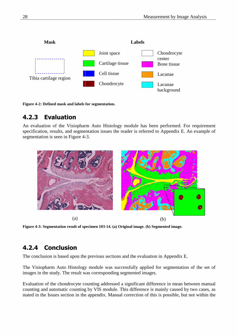
Settings for each step in the process can be defined by the user. For each type of class segmented from the image, a given label is defined. Each label is associated with a color as illustrated in the color palette in Figure 4-2. Throughout the report, the illustrated color palette is used when labeling segmented images. Furthermore a mask is used to indicate specific areas. The tibia cartilage region is indicated by a mask indicated by a blue dotted line as illustrated in Figure 4-2. An example of a segmented image labeled with this palette is seen in Figure 4-3b.
4 A filter designed for enhancing round or oval shapes.
Measurement by Image Analysis
28
Mask Labels
Joint space
Cartilage tissue
Cell tissue
Chondrocyte
Chondrocyte center
Bone tissue
Lacunae
Lacunae background
Figure 4-2: Defined mask and labels for segmentation.
4.2.3 Evaluation
An evaluation of the Visiopharm Auto Histology module has been performed. For requirement specification, results, and segmentation issues the reader is referred to Appendix E. An example of segmentation is seen in Figure 4-3.
(a)
(b)
Figure 4-3: Segmentation result of specimen 103-14. (a) Original image. (b) Segmented image.
4.2.4 Conclusion
The conclusion is based upon the previous sections and the evaluation in Appendix E. The Visiopharm Auto Histology module was successfully applied for segmentation of the set of images in the study. The result was corresponding segmented images. Evaluation of the chondrocyte counting addressed a significant difference in mean between manual counting and automatic counting by VIS module. This difference is mainly caused by two cases, as stated in the Issues section in the appendix. Manual correction of this is possible, but not within the
Tibia cartilage region

4.3 Study Module 29
specified time limit for semi automation stated by the described requirements. A high correlation was calculated for both automatic and corrected chondrocyte counting, in respect to manual counting. This indicates the difference in mean caused by a bias and this will not affect the further analysis, when comparing groups of segmented images. As stated in the Issues section in Appendix E, the segmentation and counting of chondrocytes are a hard tradeoff between different cases, and even an optimal automated solution requires minor manual correction. By these statements, the segmentation of chondrocytes performed by the module is concluded to be acceptable. Evaluation of the residual criteria pointed out that only minor manual corrections are needed in one out of four, mainly for tibia cartilage region, cartilage and chondrocyte tissue. These corrections can be performed within the specified time limit for 195 of the images. Manual corrections were possible, but not within the specified time for 4 images. Manual corrections were impossible for 2 images, which is caused by badly performed imaging. The performed segmentation is concluded to be within the criteria of semi automatic. The VIS module fulfilled the described requirements. This validates the module to be used for segmentation of the images as a preparation for the quantitative measurements of the features. The resulting segmented images from the evaluation process are not used for the analysis in this thesis. It was only meant for evaluation purpose. A study set segmented by experts at Sanofi-Aventis has been used for the analysis.
4.3 Study Module
To perform the measurements a study module was implemented in C++ using Active Template Library (ATL) as framework and Visiopharm Imaging Utilities (IU) library for general functionality and image processing. The module was implemented as a Visiopharm Custom Algorithm in VIS to gain access to the study database. The results of the measurements was exported from the module and analyzed separately by using Microsoft Excel and Matlab. The study module is neither described any more, nor is the source code included. A final solution based upon the analysis has been implemented and is described in Chapter 11.

Measurement by Image Analysis
30

Chapter 5
Defining the Measurement Model
When pathologists evaluate a microscope image of a mouse knee joint, the focus is kept on the cartilage area affected by the disease. A pathology score is given, depending on this area only, no matter how healthy the rest of the cartilage is. In the initial studies of this project better results were obtained when keeping a similar focus in the used algorithms instead of evaluating the entire cartilage area. From these results, a definition of a measurement model was proposed. The proposal was done together with Hans Gühring, Sanofi-Aventis, as a result of a meeting the on March 30, 2006, at Visiopharm (see Appendix D).
5.1 General Definition
The proposed measurement model consists of three components:
1. A boundary of the cartilage area determined by left and right bounds. 2. A base line for the measurements. 3. A left offset, which keeps the focus on the affected area in the right side of the medial tibia
region. The general idea of the measurement model definition is illustrated in Figure 5-1 and is explained in detail in the following sections. Measurements of the cartilage matrix and chondrocytes in the matrix are performed inside a Region of Interest (ROI) defined by the three components. Measurements of the subchondral bone are performed underneath the base line.
5.1.1 Cartilage Boundary
To focus the measurements on the tibia cartilage area, a boundary of this area is defined. The important part of this definition is to include all cartilage area of relevance especially effected cartilage area. This has to be weighted in contrast to including too large an area. The boundary is given by left and right bounds. The left bound is either defined using the leftmost point of the segmented tibia cartilage region indicated by a mask, or by the tibia cartilage rounding in the left side. The optimal of the two solutions are found by evaluation in the conclusion of this chapter.

Defining the Measurement Model
32
The right bound is harder to define because of the often diffuse shape and type of area in the right side. The cartilage area in the center of the joint (in the right side of the images) is not a part of the area to be measured. The guideline is then to set the right bound at the border between the tibia cartilage area and this center area. The segmentation can often be used to determine this border, but a priori information added by pathologists is needed to ensure that the affected area is included.
Figure 5-1: Medial image of specimen 103-14 with Region of Interest (ROI) indicated.
5.1.2 Base Line
A base line is used as a guideline for the performed measurements. The base line is located at the cartilage/bone interface and is oriented by the orientation of the cartilage. The base line is delimited in the ends by the left and right bounds described in section 5.1.1. The base line can either be pointed out manually or automatically calculated.
5.1.3 Left Offset
To focus the model described by the boundary and base line even more, an offset from the left bound is used. This keeps focus on the right side of the tibia, which is known to be affected the most [16]. The left offset is defined in such a way that area, which in general is healthy for all specimens in a study, are excluded from the measurements. It is of great importance to determine an optimal left offset. Also whether it is best to use the left side of the mask or the left rounding as reference is important. A study covering these topics is performed in section 5.2.
Tibia
Femur
Bounds (left/right) Cartilage mask Cartilage rounding
Left offset ROI
Base line
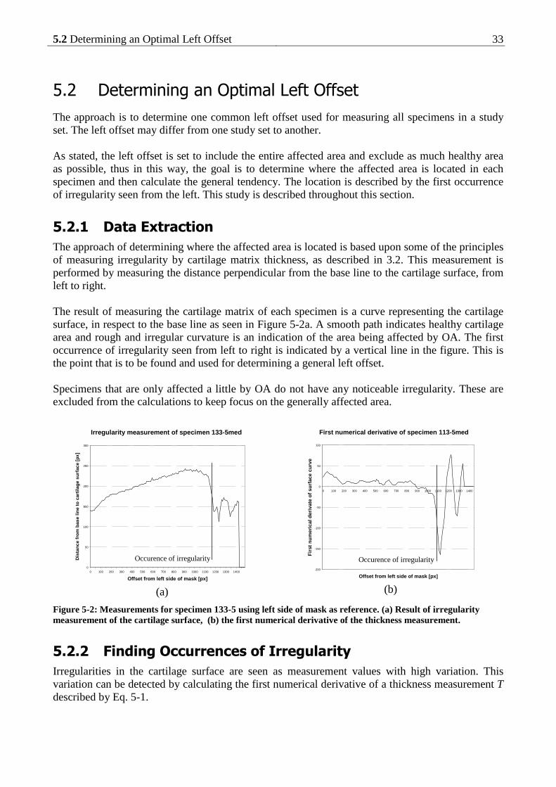
5.2 Determining an Optimal Left Offset 33
5.2 Determining an Optimal Left Offset
The approach is to determine one common left offset used for measuring all specimens in a study set. The left offset may differ from one study set to another. As stated, the left offset is set to include the entire affected area and exclude as much healthy area as possible, thus in this way, the goal is to determine where the affected area is located in each specimen and then calculate the general tendency. The location is described by the first occurrence of irregularity seen from the left. This study is described throughout this section.
5.2.1 Data Extraction
The approach of determining where the affected area is located is based upon some of the principles of measuring irregularity by cartilage matrix thickness, as described in 3.2. This measurement is performed by measuring the distance perpendicular from the base line to the cartilage surface, from left to right. The result of measuring the cartilage matrix of each specimen is a curve representing the cartilage surface, in respect to the base line as seen in Figure 5-2a. A smooth path indicates healthy cartilage area and rough and irregular curvature is an indication of the area being affected by OA. The first occurrence of irregularity seen from left to right is indicated by a vertical line in the figure. This is the point that is to be found and used for determining a general left offset. Specimens that are only affected a little by OA do not have any noticeable irregularity. These are excluded from the calculations to keep focus on the generally affected area.
Irregularity measurement of specimen 133-5med
0
50
100
150
200
250
300
0 100 200 300 400 500 600 700 800 900 1000 1100 1200 1300 1400
Offset from left side of mask [px]
Dis
tanc
e fr
om b
ase
line
to c
artil
age
surf
ace
[px]
.
(a)
First numerical derivative of specimen 113-5med
-200
-150
-100
-50
0
50
100
0 100 200 300 400 500 600 700 800 900 1000 1100 1200 1300 1400
Offset from left side of mask [px]
Firs
t num
eric
al d
eriv
ate
of s
urfa
ce c
urve
(b)
Figure 5-2: Measurements for specimen 133-5 using left side of mask as reference. (a) Result of irregularity measurement of the cartilage surface, (b) the first numerical derivative of the thickness measurement.
5.2.2 Finding Occurrences of Irregularity
Irregularities in the cartilage surface are seen as measurement values with high variation. This variation can be detected by calculating the first numerical derivative of a thickness measurement T described by Eq. 5-1.
Occurence of irregularity Occurence of irregularity

Defining the Measurement Model
34
211 −+ −=∇ ii
i
TT Eq. 5-1: First numerical derivative.
Smoothness in the derived curve yields values close to zero, and irregularities yields either high positive or negative values. To detect the first occurrence of irregularity, it is now to find the derivate values that indicate the irregularity by exceeding a certain limit. A study of solving this by using a simple threshold has been carried out in the work of this thesis. The results yielded no significant difference between the occurrences of irregularities for healthy and sick specimens. This approach is concluded to be useless for solving the problem. Inspired by quality control, the irregularities have been chosen to be detected by using the Cusum (cumulative sum) method. This method detects deviations from the expected mean, and the application is described in section 5.2.2.1. The results of applying the method is a single distance value d for each specimen, which is the distance from the reference point to the first occurrence of irregularity. Let D describe the set of all found distances d. The average µD is the average distance from the left bound to the occurrence of irregularity. It is wanted to include as much irregularity as possible, but be tolerant to outliers or extremes. For this reason a confidence level of 95% is chosen and found by subtracting two times the standard deviation σD from the average as stated by Eq. 5-2. This pushes the left offset more to the left, and guarantees the irregularities in the right side to be included as illustrated in Figure 5-4.
DDDo σµ ⋅−= 2 Eq. 5-2: Left Offset calculation.
5.2.2.1 Application of the Cusum Method For inspection of processes a various number of control charts can be used. A control scheme, which is designed to detect minor and sustained shifts in mean, is the Cusum method suggested by Page (1954) [19]. The method can be applied by the V-mask as illustrated on a measurement in Figure 5-3. The shape of the V-mask is determined by the h and k parameter. The V-mask moves along the values of the process. If any of the values violates the upper or lower arm of the V-mask, the process is detected as out of control in respect to the expected mean.

5.2 Determining an Optimal Left Offset 35
Figure 5-3: Cusum method applied by using a V-mask. The origin of the V-mask is indicated by the first point where the process is out of control by violating the upper arm. The raw data are only generated to illustrate an example.
The V-mask is complicated to implement and almost never used in practice. A tabular solution is simpler to implement, either in spreadsheet or as software functionality and is therefore preferred. The solution is based upon control of a rise or fall in values in respect to the expected mean, which is detected by calculation of the formulas Shi and Slo respectively calculated by Eq. 5-3 and Eq. 5-4. The scheme is build upon a limit parameter h and the control parameter k. During the process, if either of the two S exceeds the limit h, it indicates the process is deviating strongly from the expected mean. The k parameter controls the ability of the Cusum method to detect sustained deviation from expected mean. A low value of k makes the Cusum method sensitive to sustained deviation, based upon a long series of observations, whereas a high k value makes the Cusum method sensitive to fast and large deviations only.
Slo(i) = max(0, Slo(i-1) + µQ - k - xi) Eq. 5-3: Lower control formula, Cusum low.
Shi(i) = max(0, Shi(i-1) + xi - µQ - k) Eq. 5-4: Upper control formula, Cusum high.
Where xi is the current value of the process, µQ is the expected mean of the process Q and the control process is initialized with Slo(0) = 0 and Shi(0) = 0. Using the max() functionality adds a restart feature which makes the method sensitive to local changes in mean only. This is wanted in the case of detecting irregularities. Tuning the h and k parameter is essential to the method. Guidelines of this have been described by Vardemann [24]. It is required to define a value for the ARL (Average Run Lenght) and the size δ of critical shift in mean. The Cusum parameters can then be calculated from these values, and by use of proper Cusum tables. To define the ARL and δ, a continuous process and the properties of this process is required.
-4
-3
-2
-1
0
1
2
3
4
1 2 3 4 5 6 7 8 9 10 11 12 13 14 15 16
Raw dataCUSUM
lower arm
upper arm
origin

Defining the Measurement Model
36
From the general description of the Cusum method, a design is created to detect the occurrences of irregularities. The performed thickness measurements are finite and general ARL and δ are hard to define. For these reasons, the Cusum parameters are set empirically from observations. The irregularities are mainly negative slopes, therefore using only the Cusum low is preferred. Also a low k value is unwanted because it would make the Cusum method detect the smooth ends of healthy specimens as irregularity, which is wrong.
5.2.3 Results
The study set of 201 specimens was used. Thickness measurements were performed and first numerical derivative calculated for each specimen. From observations and a criteria of detecting as many irregularities as possible, optimal values of h=10 and k=4.5 were found. Applying the Cusum method yielded a set of D using each of the two references. Only specimens with found irregularity were included in the calculation of the left offset. The numbers of included specimens are stated by Table 5-1. The results are stated in Table 5-2.
Score (total n) 0 (11) 1 (48) 3 (43) 6 (60) 8 (39) Total (201)
Included n 0 1 4 18 27 50 Rounding
Included % 0.0 2.1 9.3 30.0 69.2 - Included n 0 1 6 40 37 84
Mask Included % 0.0 2.1 14.0 66.7 94.9 -
Table 5-1: Number of specimens with found occurrences grouped by manually given cartilage matrix pathology score. Percentages are of the total number of the given pathology score.
Cartilage Rounding
Segmented Mask
Average (µD) 1231 px 1150 px
Standard deviation (σD) 234 px 236 px
Left Offset (oD) 763 px 677 px
Table 5-2: Results of the left offset calculation.
To visually illustrate the measurements and calculations, a plot has been made combining the results in Figure 5-4. In this plot two selected measurements extremes of the cartilage surface have been plotted as curves; one healthy and one sick specimen. These plots are meant as guidelines to the scatter plot of all the measured occurrences of irregularity, which is in the top part. Notice that the placement in the y-direction is only to spread out the values and have no practical meaning. The distribution of the occurrences is also illustrated by a histogram in the bottom part.

5.2 Determining an Optimal Left Offset 37
AverageLeft Offset (-2xSTD)
Healthy
Sick
0
5
10
15
20
25
30
35
40
45
50
0 500 1000 1500 2000 2500
Offset from left side of mask [px]
His
togr
am, f
requ
ency
of i
rreg
ular
ity m
easu
res
.
Occurence of irregularity
Figure 5-4: Plot of irregularity occurrences found by using left side of mask as reference. The histogram indicates the distribution of the occurrences. Measured cartilage curves are guidelines.
AverageLeft Offset (-2xSTD)
Healthy
Sick
0
5
10
15
20
25
30
35
40
45
50
0 500 1000 1500 2000 2500
Offset from left rounding of cartilage [px]
His
togr
am, f
requ
ency
of i
rreg
ular
ity m
easu
res
.
Occurence of irregularity
Figure 5-5: Plot of irregularity occurrences found by using left cartilage rounding as reference. The histogram indicates the distribution of the occurrences. Measured cartilage curves are guidelines.
The calculated average and left offset are marked on the plot, and can be seen in respect to both the occurrences distribution and the two cartilage curves. As seen the left offset is marked through the half of the sick curve, but only at two third of the healthy curve. The result will be that a greater part

Defining the Measurement Model
38
of the healthy specimens will be measured than the sick specimens. However this will only be the case in the extremes, and the actual results will be somewhere in between.
5.2.4 Verification
Verification was carried out by selecting a subset of 30 random specimens. For each specimen the first occurrence of irregularity was determined manually and used as ground truth. Pearson’s correlation coefficient (see section 10.2) was calculated between the test set and the results for both of the applied references. A two-tailed paired Students t-test was performed to determine difference in mean. The results are stated in Table 5-3.
Manual µ D Cusum µ D Correlation coefficient
T-test p-value
Rounding 1398 1245 0.59 0.18
Mask 1233 1158 0.75 0.26
Table 5-3: Results of left offset verification.
A correlation with the manual determined occurrences was determined and no significant difference in mean was detected at a 95% level of significance for both references. Therefore, is the above described method by use of the Cusum method determined to be a good method for detecting the occurrences of irregularity.
5.2.5 Discussion of Optimal Left Offset
The standard deviation is the best indicator when comparing the results of using the two different left bounds. But the two values are approximately equal and comparing them does not point in favor of any. To make a choice, the pros and cons for the two are lined up in Table 5-4.
Pros Cons
Rounding A biological fixed point.
Is to be manually pointed out. Means more time spent and introduction of possible manual errors.
Mask Easy to acquire. Can be found automatically.
Dependent on errors in automated segmentation.
Table 5-4: Comparing pros and cons for the two possible offsets.
The main purpose of this project is to automate as much as the pathology score assessment as possible. For this reason the mask is preferred, because it uses the already developed and tested segmentation module and it makes the option of automation easy.

5.3 Discussion 39
5.3 Discussion
A model for the measurements has been defined in this chapter. Is the model correct to use for the histomorphometric measurements? The base line is an approximation of the cartilage/bone interface. By using it, noise from the highly irregular interface is removed from the measurements. This keeps focus at the cartilage surface and upper part of the cartilage matrix that are the best indicators of the level of OA affection. In addition it is a good guideline for the measurement of the subchondral bone. Observations in the study of the left offset confirmed the thesis that irregularities mainly occurs in the right side of the cartilage region. Almost none were observed in the left side. Using the left offset is seen as a good approach to delimit the area for performing measurements. Finding a good procedure to determine an optimal left offset is hard. In this chapter an approach have been described and carried out. The approach is relative cumbersome and requires optimal tuning of the applied Cusum method. For detailed analysis this approach is applicable, but in practice a rule of thumb might be a better approach to an estimated left offset. The latter proposal requires a more general study, which is not part of this thesis. A verification of using the left offset as opposite to measuring the full area has to be performed. Also the sensitivity of the optimal left offset has to be determined by performing measurements with various applied values for the left offset. These studies have been performed in the work of this thesis and are described in 10.1.

Defining the Measurement Model
40

Part II
Analysis of Methods


Chapter 6
General Measurement Details
The following chapters describe and analyze features calculated from the measurements described in Chapter 3. The methods are divided by the type of parameter of joint degradation to measure: Cartilage matrix structure, cellularity of chondrocytes or subchondral bone structure. Each measurement method is applied to the study set described in section 6.1. The strength of the performed measurements in this thesis is the possibility of sampling instead of performing an overall measurement. By sampling it is possible to analyze trends in the measurements across the specimen. The application of sampling is explained for each measurement method in the following chapters. For all measurements a sample interval of 1px was used. A set of features is calculated from the results of each measurement. The overall goal of this part is to analyze the calculated features, and determine which can be used as end points for the OA affection. For the verification a set of pathology scores manually given by pathologists at Sanofi-Aventis (see Appendix B) is used. The features are verified to be correlated with the end points using statistical methods as described in section 6.2. If a given feature is proven to be correlated with the manually given score and thereby the OA affection, the feature can be used as end point for the given parameter of joint degradation. As strong end points, the features are useful to determine the treatment effect of a given drug compound. The study set has been divided into two groups by Sanofi-Aventis; a control group and a treatment group (see Appendix A). The treatment group has been introduced to a drug compound, which might have a preventive effect against OA. The control group is used as a reference group in the verification of treatment effect. It can be determined if the drug had a positive, negative or none treatment effect by testing for significant difference between results of the two groups. This is done for all features that are approved to be strong end points.
6.1 Data Set
The applied study set are digital images of the mice in STR/1N-25-05 from Sanofi-Aventis consisting of a total of 231 images of specimens. For details about this study set and the image acquisition the reader is referred to Chapter 2. The focus of the methods is kept on the medial tibia of the dissected knee joints, and a sub set of 201 specimens of the study set have been given pathology scores for this region. Only these specimens are used when applying the quantitative measurement methods.

General Measurement Details
44
The OA influence of the mouse knee joints has been evaluated by pathologists at Sanofi-Aventis. A score for each parameter of joint degradation in the tibia region has been given for all 201 specimens in the study set using the Mankin system (see section 3.1.1). The study set has been segmented and manually corrected by Sanofi-Aventis. Further minor manual corrections were necessary to apply to most of the specimens, which included corrections of segmented cartilage tissue and outlined tibia region by using VIS mask, but only on a smaller scale. The corrections were mainly of the segmented chondrocytes and marked chondrocyte centers. These issues are known, and have been pointed out in section 4.2. The final result complies with the requirements stated in section 4.2.1. A base line at the cartilage/bone interface has been manually pointed out, for each specimen individually by pathologists at Sanofi-Aventis. This has only been done in the tibia cartilage region. The base line is used in the measurement model as described earlier. A left offset value of 677px found in section 5.2 was applied for all measurements.
6.2 Verification of Features
For verification of the calculated features statistical methods are applied. As a guideline each type of statistical method and plot are illustrated by first occurrence, to illustrate the application, and the following of the same type are put in appendix. See Appendix F, G and H. To test if results of the calculated features are correlated with the manually given pathology scores is not possible by using linear regression, because the correlation between the Mankin scoring system and the degree of OA affection is not defined to be linear [15]. Therefore another approach is used: For each feature, a hypothesis of either an overall increasing or decreasing trend is given dependent on the increase in pathology score. The trend hypothesis is verified by testing for significant differences between the results of the given feature grouped by pathology score.
Definition: A trend hypothesis describes the expected trend of a given histomorphometric feature dependent on an increase in OA affection.
Each feature is tested separately. A total number of N results for a given feature are divided into k groups, dependent on the number of pathology scores present for the related parameter of joint degradation. Basic statistics for the groups are printed in tables for each feature and the distribution of observations is illustrated by box plots.
6.2.1 Applied Statistics
The statistical methods applied for verifying the calculated features are briefly described in this section, with a focus on the specific application. All methods are part of basic statistics described in ‘Probability and Statistics for Engineers’ by Miller and Freund’s [17] or similar statistic materials.

6.2 Verification of Features 45
To determine variance between the values of the grouped data an ANOVA (ANalysis Of VAriance) test would be appropriate. The ANOVA test is not performed in this thesis though, because of a detailed comparison of differences in both mean and median are carried out by Students T-test and Mann-Whitney in this thesis.
6.2.1.1 Verification of Normal Distribution The applied statistics require the measured data to be normal distributed or approximated to normal distributed. This is verified by visual inspection of histograms and normal score plots. If the observations deviate from normal distribution, transformations may be applied to correct this.
6.2.1.2 F-test The variances of the groups are wanted to be as equal as possible. To verify this, the two-sample F-test is used. No assumptions of increase or decrease in variance are done, therefore a two-tailed F-test is used. The following is given for each combination of the groups: Null-hypothesis: σ1 = σ2 Alternative hypothesis: σ1 ≠ σ2
Level of significance: α = 0.05 The result of the F-test calculation is a p-value, which is tested against the level of significance. If the p-value is above α, the null-hypothesis is accepted and the variance is equal between the two tested groups, if not the null-hypothesis is rejected and the variances are significantly unequal. Note that the F-test assumes the observations in the two tested groups to be normal distributed. If this is not the case, the result of the F-test is unreliable.
6.2.1.3 Students T-test Significant difference in mean between each of the groups individually is tested by using an unpaired one-tailed two-sample T-test. The one-tailed T-test is chosen because assumption of the means is made by the trend hypothesis of the given feature. If the F-test for the given set of grouped data has accepted the null-hypothesis, then the T-test for equal distributions is used, otherwise the T-test for unequal distributions. The following is given for each combination of the groups: Null-hypothesis: µ1 = µ2 Alternative hypothesis: µ1 < µ2 or µ1 > µ2
Level of significance: α = 0.05 The calculated result of the T-test is a p-value, which is tested against the level of significance. If the p-value is above α, the null-hypothesis is accepted, which is against the stated trend hypothesis for the given feature. Otherwise the null-hypothesis is rejected and the means are significantly unequal. Whether µ1<µ2 or µ1>µ2 is the case is verified by the basic statistics and box plots of the grouped distributions of results. It is wanted that, as many of the combinations comply with the overall trend hypothesis of the given calculated feature as possible, especially for groups with consecutive scores.
6.2.1.4 Mann-Whitney As an alternative to the T-test, the Mann-Whitney U test (equivalent to the Wilcoxon rank sum test) is also performed. The Mann-Whitney is a non-parametric test that tests for difference in the median

General Measurement Details
46
between two distributions of data. Because it is non-parametric, the required assumptions of the distributions of data are less stringent, compared to the T-test, and are more tolerant to distributions that are not normal distributed. On the other hand the non-parametric tests are less precise for normal distributed data. Be aware that the results of the T-test and the Mann-Whitney can not be directly compared. Also Mann-Whitney is often preferred by Sanofi-Aventis in their research within this field. The Mann-Whitney test is performed for one-tailed distributions because assumption of the median is made by the trend hypothesis of the given feature.
6.2.1.5 Linear Regression The least square method is used for linear regression in this thesis by minimization of Eq. 6-2. An equation as in Eq. 6-1 for the line is determined, where a is the slope factor, b is the intersection with the y-axis and y the linear function of x described by the equation. Only the slope factor a is used in the feature calculations.
y = a·x + b Eq. 6-1: Equation for a line.
[ ]∑=
⋅+−n
iii xbay
1
2)( Eq. 6-2: Principle of Least Squares.

Chapter 7
Cartilage Matrix Structure
This chapter describes the applied methods for measuring and evaluating the parameters of the cartilage matrix structure. The chapter covers two main approaches of quantitative measurement of irregularity: one by the fibrillation in the cartilage, and another by the cartilage surface, found by sampled thickness measurements. The basis theory of the applied measurement methods is described in section 3.2 and the reader is referred to this section for background information. The calculated features have been verified by manually given cartilage pathology scores, and the methods have been used to test for preventive treatment effect of a drug compound against OA. Only the most important results are illustrated in this chapter. A full listing of all results is seen in Appendix F, and the reader is encouraged to look in the appendix when reading this chapter.
7.1 Irregularity by Fibrillation
The approach of measuring irregularity in the cartilage surface suggested by Pastoureau et al. [20] was the Fibrillation Index (FI). This is described in more detail in section 3.2.1. To refresh on the exact calculation, the formula for FI is stated in Eq. 7-1. In this thesis the FI measurement has been performed by the original approach and in addition two other approaches, proposed by this thesis, have been studied. The three approaches are described in the following paragraphs.
l
dFI =
d=Euclidian distance, l = length of surface curve.
Eq. 7-1: Fibrillation Index (FI)
7.1.1 Method Description
7.1.1.1 Full Width The original approach of the FI method, measures across the entire articular cartilage of either the femoral or tibia region. This measurement has been performed, and the results are used as reference

Cartilage Matrix Structure
48
for the other histomorphometric methods applied to measure the cartilage matrix. The FI method using full width is illustrated in Eq. 7-1.
7.1.1.2 Delimited Width The approach suggested by this thesis is to perform the FI measurement delimited by the applied measurement model. The FI is measured from the left offset at the cartilage surface and to the end of the surface curve. An illustration of this is seen in Figure 7-1. The approach was tested in the work of this thesis, but indicated no significant improvements in the correlation with OA affection compared to the original approach. For this reason, the approach is rendered superfluous, and is not described any further.
Figure 7-1: Specimen 196-14. Measuring delimited FI by the Euclidean distance and the surface curve, both indicated by jagged black lines.
7.1.1.3 Dividing into Stretches Using the advantage of fast computer processing, it is possible to split up the measured area and performs several FI measurements at minor stretches. The calculated fibrillation is then defined by a sum of the measured FI of all stretches. A study of this approach using the numbers of stretches from 2 to 20 delimited by the measurement model has been performed in this thesis. The results were observed to be more random and independent of the actual irregularity, as the number of stretches increases. For this reason this approach is not useful and is not described any further.
7.1.2 Interpretation of Measurements
By the definition of the FI, the yielded results are expected to be close to one for healthy specimen, whereas the more affected specimens have lower values towards zero. No further calculations of the results are applied before comparison.
Base line
Left offset

7.2 Irregularity by Thickness Measurement 49
7.2 Irregularity by Thickness Measurement
The degeneration caused by OA results in irregularity in the cartilage surface. This makes the irregularity a good indicator for the degree of OA. The irregularity can be measured by measuring the thickness of the cartilage.
7.2.1 Method Description
This measurement method is performed based on the applied measurement model, by the use of the base line and left offset. The thickness of the cartilage matrix is found by measuring the Euclidean distance from the base line and to the surface edge of the cartilage. This is done with a specific interval along the base line as illustrated on a segmented image by Figure 7-2. The result is a sampled curve of thickness values, which reflects the surface curve of the cartilage matrix.
Figure 7-2: Thickness measurement illustrated on segmented image of specimen 103-17. Used interval of measurements for this illustration is 60px.
The purpose of the thickness measurement is to describe the irregularities in the cartilage surface. This irregularity consists of small and large gaps. A special case for these gaps occurs when the surface is undermined by the OA affection. This case creates ambiguous possible definitions of the thickness measurement, as illustrated in Figure 7-4. In this thesis, the thickness measurement has been defined as the distance to the exact cartilage surface (Figure 7-4a). Another approach is by the sum of all cartilage tissue for each sample (Figure 7-4b), but this approach does not correctly reflect the surface curvature and is found inappropriate. A third approach is to measure the thickness as the distance to the inner curve (Figure 7-4c). This approach can cause critical failure, if small deep gaps occur as illustrated in Figure 7-3, and is for this reason not applied.
Left offset
Base line
Measured thickness
Figure 7-3: Failure by inner curvature thickness measurement.

Cartilage Matrix Structure
50
0
50
100
150
200
250
1 3 5 7 9 11 13 15
Sample no
Thi
ckne
ss m
easu
re [
px]
0
50
100
150
200
250
1 3 5 7 9 11 13 15
Sample no
Thi
ckne
ss m
easu
re [
px]
0
50
100
150
200
250
1 3 5 7 9 11 13 15
Sample no
Thi
ckne
ss m
easu
re [
px]
(a) (b) (c)
Figure 7-4: Ambiguous thickness measurement definitions. Base line and thickness measurement indicated on a cropped part of specimen 213-5. (a) To the exact surface (applied in this thesis). (b) Sum of cartilage tissue. (c) Following inner curvature.
7.2.2 Interpretation of Measurements
The measured results from the method are interpreted by statistical calculations to get a single quantitative value for the irregularity. In the following, X is used to indicate the set of values that is the result of each performed thickness measurements. The following set of hypotheses is proposed for the results of the thickness measurement depending on the two extreme levels of OA:
1. Measuring a specimen with a healthy cartilage matrix yields a smooth curve with values at a high level.
2. The measurement of a cartilage matrix, which is highly affected by OA yields a set of values with high variance at a lower level than the healthy.
Figure 7-5: Theses for thickness measurement results X of two extremes. (a) Healthy specimen. (b) Specimen highly affected by OA.
Sample no.
X
Sample no.
X
(a) (b)
Overall trend

7.2 Irregularity by Thickness Measurement 51
The two theses are illustrated in Figure 7-5. Based upon the theses, four basic statistics are candidates as features:
1. Total value of X (area under the curve) 2. Overall average of X. 3. Overall variance of X. 4. Slope of X
To measure the total value of X is equal measuring the size of the cartilage, delimited by the measurement model. The size is a composite of two parameters: the thickness of the cartilage and the width of the measured cartilage. The composition makes the results harder to interpret, because long and thin is similar to narrow and thick. The expected measurements of the specimens is somewhere in between, and hard to determine if healthy or sick. Also the size is directly dependent upon the segmentation process, which is an unwanted feature. The overall average is close related to the total value, and for the above mentioned reasons, both candidates are excluded. The residual two candidates are kept for further evaluation. The expected difference in variance and irregularity in X, depending on the degree of sickness, can be evaluated by the first derivative of X. This results in X∇ , which describes the changes in the set
of values and thereby the surface curve of the cartilage. The exact calculation of X∇ is stated in Eq. 7-2 and is found by the formula of the first numerical derivative.
211 −+ −=∇ ii
X
xx Eq. 7-2: First numerical derivative of X.
The result of this calculation is a set of derivative values, which is expected to be correlated to the degree of OA as described by the following cases:
1. A specimen with a healthy cartilage yields an X with a smooth curve, and results in values of X∇ close to zero.
2. The thesis of the right part being more affected than the left (by Meacock [16]) is the basis for this case: A specimen that is affected by OA yields an X with a smooth curve as in case 1 in the first part but a growing variance in the latter part. This will result in trend values starting in the range of zero and then a growing tendency of both positive and negative values of X∇ .
3. A strongly OA affected specimen yields an X with high variance, which yields both large negative and positive values for X∇ .
Basic statistics is chosen to evaluate the results of X∇ based on the above mentioned cases. From
experimental studies the calculation of X∇ yielded both positive and negative values with almost same magnitude for all degrees of OA. This makes the average a bad parameter and is for this reason not used for evaluation. The growing tendency of the magnitude of the values, is measured by variance, and this parameter is the best for evaluating the results of X∇ . The calculation of the sample variance of the trend is stated in Eq. 7-3.

Cartilage Matrix Structure
52
Definition: The calculation of the variance of the first numerical derivative of the thickness measure is referred to as the trend variance in the following.
( )1
1
2
var −
∇−∇=∇∑
=
n
n
ii
Eq. 7-3: Trend variance of X
To sum up, the following features are calculated and evaluated:
1. Overall variance of X. 2. Slope of X. 3. Trend variance of X (Variance of the first numerical derivative X∇ ).
7.3 Results
The described measurement methods were applied to the study set of 201 specimens. A sample interval of 1px was used. Three results of the thickness measurements have been hand picked and illustrated in Figure 7-6a. From the thickness measurements, the first numerical derivative was calculated as described earlier in this chapter. In the actual calculations the last 25 samples of each measurement were excluded from the calculations, to avoid incorrect high values of X∇ , which is caused by the drop to zero in
measured thickness values in the end. Corresponding result of X∇ results for the handpicked measurements are illustrated in Figure 7-6b.
0
50
100
150
200
250
300
1 201 401 601 801 1001 1201
Sample number (px from left offset using side of mask as reference)
Mea
sure
d di
stan
ce to
sur
face
[p
x]
800-23, score 0
931-11, score 3
296-14, score 8
-40
-30
-20
-10
0
10
20
1 201 401 601 801 1001 1201
Sample number (px from left offset using side of mask as reference)
Firs
t nu
mer
ical
der
ivat
ive
of
mea
sure
d di
stan
ce t
o su
rfac
e
800-23, score 0
931-11, score 3
296-14, score 8
(a) (b)
Figure 7-6: Results of three handpicked measurements. (a) Thickness measurement. (b) Trend variance of measurement (last 25 samples of each measurement have been excluded as explained).

7.3 Results 53
7.3.1 Correlation with Cartilage Matrix Structure Score
Measured results have been grouped by manually given cartilage pathology score (see Table 7-1). As the affection of the OA progression, the cartilage matrix is expected to degenerate from a smooth surface into irregular and missing cartilage. From this a set of trend hypothesis is proposed in Table 7-2.
Manually given pathology score
0 1 3 6 8
Number of specimens 11 48 43 62 37
Table 7-1: Specimens grouped by manually given cartilage pathology score.
Feature Trend hypothesis for stronger affection by OA
FI Value towards zero. Overall Variance An increase in values. Slope Larger negative values. LTV An increase in values.
Table 7-2: Trend hypothesis of the three cellularity features.
In this section the results of the four calculated features described earlier, are divided into groups by the manually given pathology score to test for OA dependent differences. Basic statistics and box plots for the trend variance are seen in Figure 7-7. For basic statistics of all features, the reader is referred to Appendix E.
Manually given pathology score
0 1 3 6 8
N 11 48 43 62 37
Min 0.07 0.07 0.13 0.22 1.41
Max 0.46 0.92 3.46 15.28 18.45
Mean 0.19 0.28 0.85 3.43 7.41
SD 0.10 0.17 0.80 3.12 4.31
Score 0 Score 1 Score 3 Score 6 Score 8
0
5
10
15
Tre
nd v
aria
nce
of t
hick
ness
Figure 7-7: Basic statistics for the trend variance. Results are grouped by manually given pathology score.
An observation of the basic statistics and box plot for the trend variance indicates an exponential growing trend in the variance of the values. By applying a transformation by ln, the observations are transformed to approximate equal variance. The process of this transformation is illustrated in Figure 7-8 by box plots before and after the transformation. In the following only the results of the transformed observations are used. The exact calculation is stated by Eq. 7-4.
Definition: The calculation of ln to the trend variance is abbreviated and referred to as LTV in the following.

Cartilage Matrix Structure
54
Score 0 Score 1 Score 3 Score 6 Score 8
0
5
10
15
Tre
nd v
aria
nce
of t
hick
ness
ln
→
Score 0 Score 1 Score 3 Score 6 Score 8
-2
-1
0
1
2
3
ln t
o tr
end
varia
nce
of t
hick
ness
(LT
V)
(a) (b)
Figure 7-8: Transformation by using ln to approximate normal distribution. (a) Trend variance. (b) ln to the trend variance (LTV).
( )
−
∇−∇=
∑=
1ln 1
2
nLTV
n
ii
Eq. 7-4: ln to the trend variance of X (LTV).
Distributions have been verified for the grouped results of LTV and residual features, and are concluded to be approximately normal distributed. Box plots of all features are seen in Figure 7-9.
Score 0 Score 1 Score 3 Score 6 Score 8
0.3
0.4
0.5
0.6
0.7
0.8
0.9
Fib
rilla
tion
Inde
x (F
I)
Score 0 Score 1 Score 3 Score 6 Score 8
1
2
3
4
5
6
7
8
9
Var
ianc
e of
thi
ckne
ss
(a) (b)
Score 0 Score 1 Score 3 Score 6 Score 8
-0.4
-0.3
-0.2
-0.1
0
0.1
Slo
pe o
f th
ickn
ess
Score 0 Score 1 Score 3 Score 6 Score 8
-2
-1
0
1
2
3
ln t
o tr
end
varia
nce
of t
hick
ness
(LT
V)
(c) (d)
Figure 7-9: Box plots of calculated matrix features. (a) FI. (b) Overall variance. (c) Slope. (d) LTV.

7.3 Results 55
From the differences in the mean values and by visual evaluation of the box plots for all three features, an overall as well as individual trend comply with the respective trend hypothesis for each feature. F-test, T-test and Mann-Whitney tests have been performed for all features (see Table 7-3, Table 7-4 and Appendix F) and are commented in the following. Both T-test and Mann-Whitney indicates significant difference between the grouped results of the FI feature at a 95% level of significance. This indicates a strong correlation with the trend hypothesis and thereby the level of OA impact of the cartilage matrix. This confirms that the work of Pastoureau et al [20] is applicable to the mouse model of OA. Both the variance in thickness and slope of thickness measurements yields less significant results compared with the FI. Both features are unable to distinguish between group 0 and 1. Tests results for the LTV feature indicates significant difference between the grouped results for all groups and thereby confirms the trend hypothesis for this feature. Compared to the FI feature, the LTV is better to distinguish between group 1 and 3, but worse to distinguish between group 0 and 1. The variance of the grouped results is far more equal for the LTV than the FI, which is confirmed by the F-tests.
F-test T-test
0 vs 1 1 vs 3 3 vs 6 6 vs 8 0 vs 1 1 vs 3 3 vs 6 6 vs 8
FI 0.32 0.013* 0.0025* 0.62 0.011 0.0013 <0.0001 <0.0001
Variance 0.12 0.003* 0.95 0.12 0.49 0.0002 0.0003 <0.0001
Slope 0.18 0.33 0.87 0.18 0.12 0.034 0.0077 <0.0001
LTV 0.44 0.011* 0.97 0.075 0.037 <0.0001 <0.0001 <0.0001 *These F-tests rejected the null-hypothesis at a 95% level of significance, so the corresponding T-test is performed for unequal distribution.
Table 7-3: F-test and T-test results for the three calculated features.
Mann-Whitney
0 vs 1 1 vs 3 3 vs 6 6 vs 8
FI 0.0093 0.0030 <0.0001 0.0002
Variance 0.48 0.0003 0.0003 <0.0001
Slope 0.14 0.027 0.010 <0.0001
LTV 0.028 <0.0001 <0.0001 <0.0001
Table 7-4: P-values for Mann-Whitney tests for calculated features.
7.3.2 Treatment Effect
The results of the calculated features have been grouped by control and treated specimens. Normal distribution has been verified for calculated results of both groups for all features by visual inspection of normal score plots and histograms. Basic statistics of the grouped results have been calculated. Box plots of the grouped distribution of the calculated features are seen in Figure 7-10. For more results, the reader is referred to Appendix F.

Cartilage Matrix Structure
56
Control Treated
0.3
0.4
0.5
0.6
0.7
0.8
0.9
Fib
rilla
tion
Inde
x (F
I)
Control Treated
1
2
3
4
5
6
7
8
9
Var
ianc
e of
thi
ckne
ss
(a) (b)
Control Treated
-0.4
-0.3
-0.2
-0.1
0
0.1
Slo
pe o
f th
ickn
ess
Control Treated
-2
-1
0
1
2
3
ln t
o tr
end
varia
nce
of t
hick
ness
(LT
V)
(c) (d)
Figure 7-10: Box plots of calculated cellularity features grouped by control and treated specimens. (a) FI. (b) Overall variance. (c) Slope. (d) LTV.
Students T-test and Mann-Whitney are used to test for differences between the grouped results, and thereby possible treatment effect indicated by the features. The results are stated in Table 7-5. The overall variance does not indicate any significant difference. The slope of the thickness measurement indicates a significant difference and both FI and LTV indicate a high significant difference between the control and treated group.
F-test T-test Mann-W.
Fibrillation Index 0.89 0.0017 0.00054
Overall variance 0.72 0.18 0.094
Slope 0.14 0.011 0.0031
LTV 0.67 0.00045 0.00038
Table 7-5: F-tests, T-tests and Mann-Whitney for control versus treatment group for all calculated cartilage matrix features.
7.4 Discussion
A set of quantitative features based upon thickness measurement of the cartilage matrix have been described throughout this chapter. The performed thickness measurement is strongly related to the curvature of the cartilage surface, which is the most affected part of the cartilage matrix in the perspective of OA impact. The features are statistical calculations from this measurement and are thereby also strongly related to possible OA affection. The features have been tested for validity by correlation with manually given pathology scores. The FI has been used as a reference for this validation. All proposed features complied with the

7.4 Discussion 57
respective trend hypothesis. The LTV feature performed better than the features by overall variance and slope of the thickness measurement, and was the only feature to match the FI in distinguishing between the grouped results. The second test for validity by indication of treatment effect yielded results of a significant difference between the control and treated group for both LTV and the slope of the thickness measurement. The overall variance does not indicate any significant effect. For both the T-test and Mann-Whitney, the LTV indicates a more significant treatment effect than the FI. From the study of the cartilage matrix it was found that the irregularities in the cartilage surface are by far the best indication of OA affection. Other morphometric parameters, e.g. size and thickness are concluded to be bad indicators. From the analysis performed throughout this chapter and by the results of the performed calculation, the LTV feature is concluded to be the strongest end point for indication of OA affection of the cartilage matrix. The end point is determined to be correct and validated better than the FI. Also the grouped results by the LTV have far less differences in the variances than FI, which indicate a more direct correlation with the OA affection.

Cartilage Matrix Structure
58

Chapter 8
Cellularity of Chondrocytes
This chapter covers the analysis of the change in cellularity of chondrocytes in connection with OA. The cellularity is measured by a quantitative method based upon the methods used by pathologists as described in Chapter 3. The method has been applied to the study set and both the method and the results are described in detail throughout this chapter. The calculated features from the measurements have been verified by using the manually given chondrocyte pathology score, and have been used as end points to determine the treatment effect of the drug compound tested on the study set. Only the most important results are illustrated in this chapter. A full listing of all results is seen in Appendix G, and the reader is encouraged to look in the appendix while reading this chapter.
8.1 Measurement Method
The measurement in this chapter is performed according to the applied measurement model by using a baseline and a left offset. The measurement is performed by sampling perpendicular to the base line as illustrated in Figure 8-1.
Figure 8-1: Cellularity measurement with an interval of 10px illustrated on segmented image of specimen 137-20. (a) Overview with base line and left offset indicated. (b) Detailed view of base line and perpendicular sample lines.
(a) (b)

Cellularity of Chondrocytes
60
For each sampling the following tissues have been measured:
• Chondrocyte tissue
• Chondrocyte center
• Cartilage tissue
The measurement is done by counting the number of pixels of the given type of tissue, and summed up for each sample. The measurement of the chondrocytes includes the chondrocyte centers as well. The measurement of the cartilage includes both chondrocytes and centers, since they are part of the cartilage area. The result is a set of values along the base line for each of the measured types of tissue. The cellularity is calculated from these measurements, by area fraction ρarea, which was introduced in section 3.3. To refresh on the calculation, the equation of ρarea is stated again in Eq. 3-4.
[ ]1:0, ∈= areacartilage
cellsarea A
A ρρ Eq. 8-1: Cellularity by area fraction.
8.2 Interpretation of Measurements
In the following Y is used to indicate the measurement of the cellularity measurement. From the tendencies of cellularity, the following trends of Y are expected: For the measurement of Y in case of a healthy specimen, the cellularity is expected to be high compared with the cartilage area, i.e. Y yields a set of high values (illustrated in Figure 8-2a). Because of the tendency in difference between left and right side, a measurement of a medium affected specimen has higher values in the first part of the set Y than the last (illustrated in Figure 8-2b). In case of a sick specimen, the measurement will yield a lower set of values than for a sick. The difference between left and right is less than for the medium affected (illustrated in Figure 8-2c).
Figure 8-2: Expected trends of measurement results for Y. (a) Healthy. (b) Medium affected. (c) Sick.
Sample no.
X
Sample no.
X
Sample no.
X
(a) (b) (c)
Overall trend

8.2 Interpretation of Measurements 61
By elaborating on the proposed trend thesis, two main characteristics define the difference in state of cellularity between the three degrees: overall mean and overall trend. From these characteristics, three approaches for evaluation have been proposed and applied. The first and most simple approach is by calculating the average of all the cellularity samples for each specimen individually. This yields a single average value Y for each specimen as stated in Eq. 8-2.
n
YY
n
ii∑
== 1 Eq. 8-2: Average of cellularity.
Where n is the number of samples in the measurement. The second feature is based upon the thesis of difference in overall trend. This difference is found by fitting a line through the samples by linear regression as explained in section 6.2.1.5 and measuring the slope of the line. A healthy specimen will result in a slope value close to zero and a sick will result in a large negative slope value. An exception occurs by using this approach: if the specimen is strongly sick, the cellularity will be overall low in both sides and the slope value will only be slight negative. To compensate for this case, the calculated slope is normalized by the calculated average value of the specimen. This yields the formula in Eq. 8-3. Performed tests during this project have indicated an improvement in difference between specimens at different stages.
Y
aS Y
Y = Eq. 8-3: Normalized slope
Where Ya is the slope coefficient in the function of the fitted line: y = a·x + b. A third approach is by evaluating the measurement Y for each sample by using a given threshold value t as illustrated in Figure 8-3. The exact calculation is the count of samples above the threshold normalized by the total number of samples as stated in Eq. 8-4. The results will yield values close to 1 for healthy specimens and values towards 0 the more affected the specimens are. The calculation is an expression of the percentage of the full cartilage that contains enough chondrocytes to be classified as healthy.
n
tyIT
n
ii
Y
∑=
>= 1
)(
Eq. 8-4: Evaluation by threshold.
Where t is the defined threshold value and I is an indicator function, which is 1 when the condition is true and 0 otherwise.
Sample no.
Y
TY 1 1 1 0 0 1 0 0 0
t
Figure 8-3: Threshold evaluation illustrated.

Cellularity of Chondrocytes
62
Three approaches for defining the threshold were suggested: 1. Single average – One overall average value is calculated for the all the measurements of the
entire study. 2. Individual averages – An average value is found for each measurement and used as threshold
only for the given. The idea is to make it possible to evaluate a single measurement separately without results from the entire study as in the first suggestion.
3. Multiple averages – An average is found for each sample slot across all of the measurements. This result in a vector of average values. A line is fitted through the calculated values, and values from the line are used specific for each sample slot. The idea of this approach is to create a general model of the sampled cellularity.
The first approach is the simplest. It is stable and yielded results with high correlation to the manually given pathology score. These results are specified later in this chapter. The second approach is too dependent on the given measurement and therefore a bad indicator of the absolute OA level. The third is more sophisticated by fitting a line as a model to the general sampled cellularity. Unfortunately this approach might remove some of the information indicating the level of affection, and the yielded results were good, but had far less significant correlation with the manually given pathology score than the first. For the mentioned reasons the second and third approach has been excluded and are not described any further. To sum up, the following features are calculated from the cellularity measurement:
1. Overall average for each specimen. 2. Normalized slope of measurement for each specimen. 3. Threshold by one overall average value for all specimens.
8.3 Results
The described measurement was performed on the study set of 201 specimens. The cartilage area has been calculated for all measurements, and three handpicked results are seen in Figure 8-4. Measurement of chondrocyte area is seen in Figure 8-5. The plots are of a handpicked specimen from each pathology score group, to make it possible to compare distinctive features that separate the groups. Figure 8-4: Measured cartilage area for selected specimens.
0
50
100
150
200
250
300
350
1 201 401 601 801 1001
Sample
Mea
sure
d ca
rtila
ge a
rea
[px]
Specimen 262-11, score 0
Specimen 133-5, score2
Specimen 760-14, score5

8.3 Results 63
05
101520
2530
3540
1 201 401 601
Sample
Mea
sure
d ch
ondr
ocyt
e ar
ea
[px]
05
1015
2025
3035
40
1 201 401 601
Sample
Mea
sure
d ch
ondr
ocyt
e ar
ea
[px]
05
1015
2025
303540
1 201 401 601
Sample
Mea
sure
d ch
ondr
ocyt
e ar
ea
[px]
(a) (b) (c)
Figure 8-5: Measured chondrocyte area for selected specimens. (a) Specimen 262-11, score 0. (b) Specimen 133-5, score 2. (c) Specimen 760-14, score 5.
The cellularity by area fraction ρarea has been calculated from the measurements, and a plot handpicked measurements is illustrated in Figure 8-6.
0
0.05
0.1
0.15
0.2
1 201 401 601 801 1001
Sample
Cho
ndro
cyte
are
a fr
actio
n
Specimen 262-11, score 0
Specimen 133-5, score2
Specimen 760-14, score5
0
0.05
0.1
0.15
0.2
1 201 401 601 801 1001
Sample
Sm
ooth
are
a fr
actio
n
Specimen 262-11, score 0
Specimen 133-5, score2
Specimen 760-14, score5
(a) (b)
Figure 8-6: Cellularity by area fraction ρarea for a selected specimen. (a) Original measurement. (b) Smoothed measurement to ease interpretation of measurement. A 1D Gauss kernel by the size of 30 samples was applied.
A problem with spikes occurs in the cellularity calculation. In some cases the specimen contains a relative high value of chondrocyte area in relation to cartilage area in the last samples of a specimen. In these cases, the cartilage area is close to zero, so the results of the calculations are extremely high values, compared to the general results. This problem is illustrated by Figure 8-7. To compensate for this problem, the last n samples are excluded from the calculations. The number of samples to exclude is empirically set from observation of the given study. A proper number for the study at hand is 15 sample slots to exclude.

Cellularity of Chondrocytes
64
0
0.1
0.2
0.3
0.4
0.5
50 45 40 35 30 25 20 15 10 5
Last sample number
Cho
nd
rocy
te a
rea
frac
tion
Figure 8-7: Spike problem illustrated by last 50 samples of all chondrocyte area fraction calculations. Exclusion of last 15 samples is illustrated by a vertical red dotted line.
By known fact there will be a decreasing trend in the number of chondrocytes as the disease progresses. From this fact trend hypothesis are stated for all three features in Table 8-1.
Feature Trend hypothesis for stronger affection by OA
Overall average A decrease in mean.
Normalized slope Larger negative values.
By threshold Value towards zero.
Table 8-1: Trend hypothesis of the three cellularity features.
8.3.1 Correlation with Chondrocyte Score
Measured results have been grouped by manually given chondrocyte pathology score (see Table 8-2). Normal distribution has been verified for calculated results of all groups for all calculated features by visual inspection of normal score plots and histograms. Basic statistics of the grouped results have been calculated. Box plots of the grouped distribution of the calculated features are seen in Figure 8-8.
Score 0 Score 2 Score 50.01
0.02
0.03
0.04
0.05
Ave
rage
cel
lula
rity
Score 0 Score 2 Score 5
-3
-2
-1
0
1
2
x 10-3
Slo
pe o
f ce
llula
rity
Score 0 Score 2 Score 5
0.2
0.3
0.4
0.5
0.6
0.7
0.8
Cel
lula
rity
by t
hres
hold
(a) (b) (c)
Figure 8-8: Box plots of calculated cellularity features. (a) Overall average. (b) Normalized slope. (c) By threshold.
Exclusion limit

8.3 Results 65
Manually given pathology score
0 2 5
Number of specimens 9 152 40
Table 8-2: Specimens grouped by manually given chondrocyte pathology score.
From the basic statistics a decrease in mean values for the overall average feature confirms the trend hypothesis, which is also seen from the corresponding box plot. The trend hypothesis for both the normalized slope and the threshold feature is also confirmed by their respective basic statistics and box plots. Performed T-tests indicates significant difference in mean on a 95% level of significance between all groups for each of the three features individually. The p-values for F-tests and T-tests are stated in Table 8-3. Additionally the Mann-Whitney was performed, which indicated significant difference between the medians of the grouped results. Calculated p-values for Mann-Whitney are stated in Table 8-4.
F-test T-test 0 vs 2 2 vs 5 0 vs 5 0 vs 2 2 vs 5 0 vs 5
Overall average 0.197 0.0004* 0.648 0.0001 <0.0001 <0.0001 Normalized Slope 0.0004* 0.75 0.0007* <0.0001 <0.0001 <0.0001 By threshold 0.0091* 0.10 0.045* <0.0001 <0.0001 <0.0001
*These F-tests rejected the null-hypothesis at a 95% level of significance, so corresponding T-test is performed for unequal distribution.
Table 8-3: P-values for both F-test and T-test for all combinations of groups for each of the features.
Mann-Whitney 0 vs 2 2 vs 5 0 vs 5
Overall average 0.0001 <0.0001 <0.0001 Normalized Slope 0.0004 0.0034 <0.0001 By threshold <0.0001 <0.0001 <0.0001
Table 8-4: P-values for Mann-Whitney tests for calculated features.
8.3.1.1 Smoothing A study of smoothing the measurements to improve the separation of the grouped data has been performed. A 1D gauss kernel at various sizes was convoluted with the measurements. The smoothing did improve the results of the normalized slope and cellularity by threshold, at large kernel sizes (100px-200px), but not remarkable and smoothing is seen as superfluous.
8.3.2 Treatment Effect
In the previous section all three features were proven to be good indicators for the level of affection by OA. This makes them useful for determining the treatment effect of a given drug compound. The calculated results are divided into groups by control and treated. Normal distribution has been verified for calculated results of both groups for all features by visual inspection of normal score plots and histograms. Basic statistics of the grouped results have been calculated. Box plots of the grouped distribution of the calculated features are seen in Figure 8-9.

Cellularity of Chondrocytes
66
Control Treated0.01
0.02
0.03
0.04
0.05
Ave
rage
cel
lula
rity
Control Treated
-3
-2
-1
0
1
2
x 10-3
Slo
pe o
f ce
llula
rity
Control Treated
0.2
0.3
0.4
0.5
0.6
0.7
0.8
Cel
lula
rity
by t
hres
hold
(a) (b) (c)
Figure 8-9: Box plots of calculated cellularity features grouped by control and treated specimens. (a) Overall average. (b) Normalized slope. (c) By threshold.
Students T-test and Mann-Whitney are used to test for difference between the grouped results, and thereby possible treatment effect indicated by the features. The results are stated in Table 8-5. The tests for both the overall average and cellularity by threshold, do not agree if there is any significant treatment effect on a 95% level of significance. The normalized slope indicates a highly significant treatment effect indicated by both the T-test and Mann-Whitney.
F-test T-test Mann-W.
Overall average 0.22 0.070 0.030
Normalized Slope 0.97 0.0002 0.0004
By threshold 0.03* 0.206 0.047 *These F-tests rejected the null-hypothesis at a 95% level of significance, so corresponding T-test is performed for unequal distribution.
Table 8-5: F-tests, T-tests and Mann-Whitney for control versus treatment group for all three calculated cellularity features.
8.4 Discussion
A set of quantitative features, describing the cellularity of the chondrocytes in the articular cartilage, has been presented in this chapter. The features are calculated from a measurement based upon area fraction of the chondrocyte area in respect to the cartilage area. This measurement is strongly related to the cellularity volume fraction, and thereby a strong measure of the spatial cellularity in the cartilage matrix. Decrease in the cellularity caused by OA influence can therefore be measured by this area fraction. Argumentation for these statements are performed in section 3.3. All three proposed features indicated a significant correlation to the manually given pathology score, which is seen as the truth of OA affection. The overall average of the cellularity did not indicate any significant treatment effect on a 95% level of significance. This makes this feature a weak end point for assessment of OA influence on cellularity. The cellularity by threshold is as good as the overall average cellularity, but the feature requires a proper threshold value to be set. This is seen as a disadvantage, and no advantages are seen compared to the overall average feature. Additionally did this feature not indicate the expected

8.4 Discussion 67
treatment effect. For these reasons the cellularity by threshold is not seen as a good end point for OA affection of the chondrocytes. The normalized slope of the measured cellularity indicated a highly significant treatment effect. This confirms the hypothesis of a difference in cellularity of the left and right side caused by the OA affection. To elaborate on this, the results can be seen as an OA stage dependent fact, that the cellularity is affected in advance of the cartilage matrix degradation. This fact can be confirmed even more by an age dependency study that describes the development process of the OA disease. Such a study has been carried out in this thesis and is described in Chapter 12.

Cellularity of Chondrocytes
68

Chapter 9
Subchondral Bone Structure
This chapter covers the analysis of the thickening process of the subchondral bone, caused by OA. The process is examined by changes in the bone density of the subchondral bone. The applied method for measuring the bone density is generally described in Chapter 3. Two features are calculated from the measurement and used in the analysis. The measurement method has been applied to the study set, and both the method, the features and the results are described in detail throughout the chapter. Only the most important results are illustrated in this chapter. A full listing of all results is seen in Appendix H, and the reader is encouraged to look in the appendix when reading this chapter.
9.1 Measurement Method
The measurement of the bone density is performed by measuring the area of bone tissue underneath the articular cartilage in respect to the total area. This is stated by Eq. 3-5.
[ ]1:0, ∈= BoneTotal
BoneBone A
A ρρ Eq. 9-1: Bone density.
The measurement is performed inside a rectangular box, which is aligned to the base line used in the measurement model. The box is defined by a length given by the measurement model and with a fixed height. To include as much information as possible, the fixed height is given as the largest possible distance from the base line to the bottom border of the image. The smallest of the largest possible distances from all the specimens in the study set is found, and is used in all the bone density measurements applied to the study set. To include the entire cartilage/bone interface area, the box is extended by a top offset. The top offset is empirically set and used for all the performed bone density measurements. The measurement method is illustrated in Figure 9-1, where segmented tissue, measured as bone, is indicated by black. Other measured tissue is indicated by white, and tissue that is not included in the measurement is by individually given original color. A description of which types of tissues that are measured is found in section 3.4.1. The area inside the box is measured in lines perpendicular to the base line. This is done by sampling with steps of 1 px, and results in a set of sample values describing the bone density along the line.

Subchondral Bone Structure
70
Figure 9-1: Performing subchondral bone measurement on segmented image of specimen 174-14. Base line and left offset from the measurement model is indicated. #1 Top offset. #2 fixed box height.
9.2 Interpretation of Measurements
In the following, Z is used to indicate the set of sampled bone density measurements for an arbitrary specimen. The first feature from the measurement is the overall average of the bone density. The calculation of this feature is defined by Eq. 9-2.
n
ZZ
n
ii∑
== 1 Eq. 9-2: Average of bone density.
Where n is the number of samples in the measurement. From the known fact that the OA affection starts in the right side of the specimens, the following statements of the bone density dependent on the OA affection is given:
• A healthy specimen will have an equally distributed bone density. • An affected specimen will have a higher bone density in the right side. • A highly affected and sick specimen will have a generally higher bone density and almost
completely bone tissue in the right side. From these statements, the slope of the measurement Z is seen as an interesting feature to calculate and use as end point for the condition of the subchondral bone. The slope of Z is found by linear regression (section 6.2.1.5) of the values in Z. The trend hypothesis is that there will be a growing trend of the average bone density as the disease progresses i.e. the higher pathology score, the higher bone density. The trend hypothesis for the slope of the bone density is a rise in values as the pathology score values increase.
#1
#2 Base line
Left offset

9.3 Results 71
9.3 Results
The described measurement was performed on the study set of 201 specimens. The largest possible height of the measurement box was calculated to 459px, and the top offset was empirical set to 100px. Both setup values were used for all the measurements in the study set. An example of the result of a bone density measurement is illustrated by Figure 9-2, which can be related to the segmented image in Figure 9-1.
0
0.1
0.2
0.3
0.4
0.5
0.6
0.7
0.8
0.9
1
1 101 201 301 401 501 601
Sample from left offset [px]
Bon
e de
nsity
0
0.1
0.2
0.3
0.4
0.5
0.6
0.7
0.8
0.9
1
1 101 201 301 401 501 601
Sample from left offset [px]
Bon
e de
nsity
(a) (b)
Figure 9-2: Bone density measurements. (a) Specimen 174-17, score 0. (b) Specimen 862-20, score 8
9.3.1 Correlation with Bone Score
Measured results have been grouped by manually given bone pathology scores (see Table 9-1). Normal distribution has been verified for calculated results of all groups for both end points by visual inspection of normal score plots and histograms. A slight skew of the distributions of the overall average was seen. Because of this, the Mann-Whitney results are preferred in favor of the T-test for this feature. Basic statistics of the grouped results have been calculated. Box plots of the grouped distribution of the calculated features are seen in Figure 9-3.
Score 0 Score 3 Score 8
0.4
0.5
0.6
0.7
0.8
0.9
1
Ave
rage
bon
e de
nsity
Score 0 Score 3 Score 8
-5
0
5
10
15x 10
-4
Slo
pe o
f bo
ne d
ensi
ty
(a) (b)
Figure 9-3: Box plots of measured subchondral bone features grouped by manually given pathology score. (a) Average bone density. (b) Slope of bone density.

Subchondral Bone Structure
72
Manually given pathology score
0 3 8
Number of specimens 4 92 105
Table 9-1: Specimens grouped by manually given bone pathology score.
From the differences in the mean values for the average bone density and by visual evaluation of the box plots, an overall as well as individual positive trend of the density values confirms the trend hypothesis. The performed T-tests indicate significant differences in mean between each of the groups. A significant difference between the groups is also confirmed by the Mann-Whitney test at a 95% level of significance. The trend hypothesis for the slope of the bone density is confirmed by the same facts. Also both the T-tests and Mann-Whitney indicates significant differences between the groups for this feature at a 95% level of significance. P-values of the F-tests and T-tests are seen in Table 9-2. Additional results for Mann-Whitney test for difference in median is stated in Table 9-3.
F-test T-test 0 vs 3 3 vs 8 0 vs 8 0 vs 3 3 vs 8 0 vs 8
Overall average 0.232 0.021* 0.418 0.0003 <0.0001 <0.0001
Slope 0.013* 0.015* 0.026* <0.0001 0.0234 <0.0001 *These F-tests rejected the null-hypothesis at a 95% level of significance, so corresponding T-test is performed for unequal distribution.
Table 9-2: P values for F-test and unpaired one-tailed T-test performed on the grouped feature results.
Mann-Whitney 0 vs 3 3 vs 8 0 vs 8
Overall average 0.0015 <0.0001 0.0004
Slope 0.030 0.024 0.0029
Table 9-3: P-values for Mann-Whitney tests for calculated features.
9.3.2 Treatment Effect
The calculated values have been grouped by control and treated specimens. Normal distribution has been verified for calculated results of both groups for both end points by visual inspection of normal score plots and histograms. Basic statistics of the grouped results have been calculated. Box plots of the grouped distribution of the calculated features are seen in Figure 9-4. For more results, the reader is referred to Appendix H.

9.4 Discussion 73
Control Treated
0.4
0.5
0.6
0.7
0.8
0.9
1
Ave
rage
bon
e de
nsity
Control Treated
-5
0
5
10
15x 10
-4
Slo
pe o
f bo
ne d
ensi
ty
(a) (b)
Figure 9-4: Box plots of measured subchondral bone features grouped by control and treated. (a) Average bone density. (b) Slope of bone density.
By performing an F-test it was seen that the two groups of data are equal distributed for only the overall average, but not for the slope (see Table 9-4). An expected effect of the treatment will yield a lower bone density and a lower slope value for the treated group. Both trend hypotheses were confirmed by a significant difference in mean tested by T-tests on a 95% level of significance using a one-tailed T-test. The results of Mann-Whitney indicate significant difference between the medians for both features.
F-test T-test Mann-W.
Overall average 0.11 0.0036 0.00752
Slope <0.0001* 0.0121 0.037 *These F-tests rejected the null-hypothesis at a 95% level of significance, so corresponding T-test is performed for unequal distribution.
Table 9-4: F-tests, T-tests and Mann-Whitney for control versus treatment group.
9.4 Discussion
A pair of quantitative features for determining the condition of the subchondral bone has been presented in this chapter. Both features were found to be significantly correlated to the manually given pathology score and thereby the level of OA affection of the subchondral bone. In addition, both features indicated a difference between the control and the treated group, which then indicates an effect of the treatment. This was proven by both the Students T-test and by the Mann-Whitney test. The group of score 3 has a remarkably higher standard deviation than the other two for both features. These deviations are addressed to doubts by the pathologists when assigning pathology score, because it is rather easy to manually distinguish between a fully healthy (score 0) or a very sick specimen (score 8 and above), but in between is harder.

Subchondral Bone Structure
74
The group of score 0 contains only 4 specimens, which makes the use of statistics unreliable. It has to be noticed that this group had by far the smallest standard deviation, in both the case of overall average and slope of bone density measurement, which adds to the precision. The lacunae areas are large blobs in the bone tissue. The variation of these only has minor influence on the average bone density, whereas the slope of the bone density is highly dependent on the placement and sizes of each individual lacuna. From the box plots and basic statistics of the latter feature, it is seen that the results of group 3 overlaps the other groups. As mentioned, this is partly caused by inaccuracy of the manual assessment, but this can also be due to inaccuracy in measurements by this feature. Even though the statistical tests indicated significant results for the slope feature, this feature is not seen as reliable. The average bone density is a simple and strong feature, which is concluded to be the best end point for the OA influence of the subchondral bone. A more sophisticated feature based upon the composition of the lacunae and subchondral bone plate is a possible end point for the condition of the subchondral bone. This is not a part of this thesis, but is addressed further in Chapter 14.

Chapter 10
Method Analysis Evaluation
This chapter sums up on the results and discussions from the previous three chapters. For each of the parameters of joint degradation, an optimal end point has been selected:
• Irregularities in the cartilage matrix by ln to the trend variance of the thickness measurement (LTV).
• Cellularity by slope of area fraction measurement.
• Bone density by average bone area fraction.
The end points have been validated by correlation with the manually given pathology score and found applicable for determining treatment effect. An overall elaboration of the treatment effect indicated by these end points is performed in section 10.3. Possible correlation of the three end points and the meaning of this are examined in section 10.2. The necessity of a verification of the applied left offset was pointed out in section 5.3 and is performed in section 10.1. A further validation can be performed by studying the correlation with expected age dependent trends of the OA disease. This study has been performed in this thesis and is described in Chapter 12.
10.1 Verification of Left Offset
A study varying the value of the applied left offset was performed. Values in the range 0px to 1334px (two times the optimal) was applied in the study. The calculated p-values for the T-tests and Mann-Whitney were used to evaluate performance of the end points. The calculated offset was useful for the cartilage matrix structure, but the cellularity indicated that a lower offset would be better. The reason is that the offset is found by the first occurrence in irregularity in the cartilage surface. Because the cellularity is often affected at an earlier stage than the cartilage matrix, the occurrences of cellularity affection is more to the left (lower left value) than the ones of cartilage irregularity. The bone density was not influenced noticeably by the changes of the left offset.
Method Analysis Evaluation
76
A variation of the applied left offset had in general only a little influence on the significance of the statistical tests. By this study, it was found that the precision of the applied left offset is of low importance. Using a left offset is still recommended to keep a focus on the most affected area of the tibia region.
10.2 Overall Correlation
The correlation between the parameters of joint degradation is calculated to examine the relationship between the parameters. The observations are approximately normal distributed therefore the correlation is preferred to be determined by the parametric Pearson correlation coefficient r, which indicates the linear correlation between two set of observations. This coefficient values is calculated by the formula in Eq. 10-1 by [17] and the value of the coefficient is in the range -1.0 ≤ r ≤ 1.0 indicating the following:
• -1.0 to -0.7 indicates a strong negative relationship between the two variables. • -0.7 to -0.3 indicates a weak negative relationship. • -0.3 to 0.3 indicates little or no relationship i.e. the variables are independent of each other. • 0.3 to 0.7 indicates a weak positive relationship. • 0.7 to 1.0 indicates a strong positive relationship between the two variables.
∑=
−−−
=n
i y
i
x
i
s
yy
s
xx
nr
1
))((1
1 Eq. 10-1: Pearson's r coefficient.
Where X and Y are the two set of observations to test for correlation, with n observations in each set. A p-value can be determined from the r coefficient by testing the null-hypothesis of r=0 with n-2 degrees of freedom by the test statistic in Eq. 10-2. The two-tailed p-value is then determined by P(T=t) = P(T>t) + P(T<-t) given by the T probability density function. If the p-value is lower than a significant limit, then the null hypothesis is rejected and the correlation is seen as significant by the given level of the limit.
21
2
r
nrt
−−= Eq. 10-2: Test statistic for r coefficient.
The calculated results for each end point have been plotted pairwise in Figure 10-1 with corresponding correlation coefficients and p-values in Table 10-1.

10.3 Treatment Effect 77
Pearson’s
r coefficient p-value
Cartilage and cellularity -0.55** <0.0001
Cartilage and bone 0.51** <0.0001
Cellularity and bone -0.28* <0.0001
Table 10-1: Correlation coefficients for correlation between the end points of each parameter of joint degradation.
-5 0 5-4
-3
-2
-1
0
1
2
3
4x 10
-3
ln to trend variance of thickness (LTV)
Slo
pe o
f ce
llula
rity
-5 0 50.2
0.4
0.6
0.8
1
1.2
ln to trend variance of thickness (LTV)
Ave
rage
bon
e de
nsity
-4 -3 -2 -1 0 1 2 3
x 10-3
0.2
0.4
0.6
0.8
1
1.2
Slope of cellularity
Ave
rage
bon
e de
nsity
(a) (b) (c)
Figure 10-1: Pairwise scatterplots of the end points. (a) Cartilage and cellularity. (b) Cartilage and bone. (c) Cellularity and bone.
From the results of the Pearson correlation it is seen that the condition of the cartilage matrix is correlated to both the cellularity and the subchondral bone parameters determined by the calculated end points. This means that a specimen with and irregular cartilage matrix also has an affected cellularity and/or the bone, and visa versa. From the correlation tests it can not be determined which causes the other, only that a correlation exists. The value of the correlation coefficient between the cellularity and the bone is noticeable lower, and indicates only a little relationship. This means that a specimen with an OA affected subchondral bone, does not necessarily have an affected cellularity and visa versa, it does occur in some cases though, but this is addressed to other conditions.
10.3 Treatment Effect
Overall, the cartilage matrix and cellularity end point indicated the same significance of treatment effect, but the subchondral bone end point was lower compared to the other (see Table 10-2). This is caused by either of three reasons, or a combination:
1. OA at the stage of this study has affected the parameters of joint degradation differently. 2. The applied methods have differences in validity and correctness. 3. The used drug compound influences the parameters of joint degradation differently.

Method Analysis Evaluation
78
It is hard to determine which and to be able to conclude if the found treatment effect is correct. It has to be confirmed by other validated standard end point and by the use of other drug compounds with known effect.
T-test Mann-Whitney
LTV 0.00045 0.00038
Slope of cellularity 0.0002 0.0004
Bone area fraction 0.0036 0.00752
Table 10-2: Summarizing the treatment effect results for end points of each parameter of joint degradation.

Part III
Application


Chapter 11
Implemented Solution
11.1 Introduction
A software module has been designed and developed to prove the applicability of the proposed end points. Additionally the module is seen as a prototype module, which can be further developed for pathologist users at companies, as for example Sanofi-Aventis. Requirements for the module are stated in 11.1.1. Requirement analysis of the requirements has been carried out to determine an optimal design and implementation of these. A set of tools for Object Oriented Analysis and Design (OOAD) presented by Larman in [11] have been selected for the analysis and design of the module. Only tools and principles of high relevance have been used because of the limited scale of the developed software. The tools are briefly described in the first part of section 11.2 and 11.4.2, and application of these is described subsequently. In descriptions of the tools, the applied terms are emphasized to make it easy for the reader to identify and understand the tools. When reading this chapter it is assumed that the reader knows the end points, which have been concluded to be measured in Part II. An understanding of the images in the study set and corresponding segmented images is also assumed. Also the measurement model described in Chapter 5, including the terms of base line and left offset are to be known.
Definition: The developed module is referred to as the “OA Quantifier module” throughout the thesis.
11.1.1 Requirements
The module is designed within the scope of this thesis, which gives the following prerequisites:
1. As input a study set of specimens is expected. Each specimen is a microscope image of medial histological sections.
2. Correct segmentation of the images is a prerequisite. Requirements for the segmentation are described in section 4.2.

Implemented Solution
82
The following goals are set for the module:
3. The module has to be semi automatic with as little interaction and required work by the user as possible.
4. Time of processing is not critical but has to be acceptable for the user. 5. Following proposed end points are to be calculated automatically for each specimen.
a. Cartilage Matrix Structure i. Fibrillation Index (FI)
ii. Ln to the variance of the first numerical derivative of thickness measurement of the cartilage (LVT).
b. Chondrocyte Cellularity i. Overall average of chondrocyte area fraction (CCV).
ii. Cellularity by slope (CCS) c. Subchondral Bone Structure
i. Overall average of bone volume (SBV). 6. For the measurement model the following needs to be cleared:
a. Calculation of a general left offset for the given study set. b. Defining an individual base line for each specimen.
The module is required to match the software guidelines and framework used by Visiopharm. By these guidelines the following requirements are stated:
7. The module has to be implemented as a part of the Visiopharm VIS software. 8. The module has to be embedded in a DLL with a given interface by VIS standard. 9. The module has to be programmed in C++. 10. The solution should take advantage of Visiopharm IU (Imaging Utilities) functionality. 11. The development must be based upon the ATL (Active Template Library) framework.
A description of the Visiopharm VIS software is given in section 11.1.2. A description of Visiopharm IU is given in section 11.1.3. The measurements are only performed on the tibia region.
11.1.2 Visiopharm Integrator System
The Visiopharm Integrator System (VIS) is the main product of Visiopharm A/S. The software is mainly developed for aiding life science research with image analysis. The structure of VIS is build to reflect the workflow of this type of work, with individual modules for image acquisition from microscope, various image analysis tools, and statistical tools for analysis of results. The user can either perform analysis on a single image or run a batch process on a study set. Both the images and results from analysis calculations are stored in a database. The structure of VIS is illustrated in Figure 11-1. The user interacts with VIS using a Microsoft Windows
Figure 11-1: The overall structure of the VIS software. Borrowed from [25].

11.1 Introduction 83
based graphical user interface. A screenshot from the running application is seen in Figure 11-2.
Figure 11-2: Screenshot from running VIS software using the Segmentation module. The following areas are indicated on the screenshot: (1) Module bar. (2) Toolbar. (3) Work area. (4) Card view of study in VIS database.
11.1.3 Visiopharm Imaging Utilities
For general image processing purposes, Visiopharm have developed the Imaging Utilities SDK (IU-SDK). It offers a set of basic data structures for storing matrix and bitmap data, with numerous methods for manipulating and managing memory for these types. A layer of basic image algorithms uses these data types for carrying out image analysis functionality e.g. classification, filtering and geometric measuring. Some improved standard functionality is included as well such as random values, rounding, FIFO list and file management. A layer of advanced algorithms is on top of the basics taking advantage of the subjacent functionality. Most of these algorithms concern general image processing. Visiopharm have used the IU-SDK as foundation for the VIS software. The SDK is distributed along with the VIS software as well and can be implemented by the costumer in their own stand-alone imaging solutions. In this project the IU-SDK has been used to develop the software functionality used in the histomorphometric analysis. This work process has made the integration of the OA Quantifier module straightforward.
3
1
4
2

Implemented Solution
84
11.2 Requirement Analysis
The initial requirement analysis is carried out by using some of the OOAD tools as stated in the introduction of this chapter. First step in the analysis is to clarify the actors, who interacts with the module. The goals of the actors are defined by the requirements described in section 11.1.1. To determine the overall process of using the module use cases are used. Use cases are written stories, which describe the needed work of the actors to fulfill the goals. Each step in this process can then be analyzed and optimal implementation can be determined.
11.2.1 Actor Definition
In this project only one actor is active; the pathologist. He is used to be working with VIS in general as part of the pre-clinical research. His intention is to evaluate the degree of sickness of each mouse in a set of mice. Images of the left knee joint of the left hind leg have been taken by microscope as described in section 2.3. These images are imported in VIS and used for the evaluation of the mice. The goal of evaluating each image is a set of quantitative measures for each end point. He expects the evaluation process to be as automated as possible by minimizing time spend on trivial procedures. The possibility of manual guidance is wanted though, to perform minor corrections and to add known a priori information.
Definition: The pathologist actor is the only user of the system and is referred to as ‘the user’ throughout the chapter.
11.2.2 Use Case
A use case is used to describe the overall work flow performed by actors in the system. In this analysis, a use case is defined describing the work performed by the pathologist user. This use case requires a study set of images, which has been correctly segmented as stated as prerequisites in the requirements. The use case is given by the following success scenario:
1. The user manually defines individual base lines for each specimen using VIS functionality. 2. An optimal value for the left offset is calculated by using the OA Quantifier module. 3. Following specific parameter, which are related to end point calculations, is calculated by
using the OA Quantifier module: a. Max box height for SBV
4. The following end points are calculated by using the OA Quantifier module: a. Fibrillation Index (FI) b. Ln to the variance of the first numerical derivative of thickness measurement of the
cartilage (LVT) c. Overall average of chondrocyte area fraction (CCV). d. Cellularity by slope (CCS) e. Overall average of bone volume (SBV)
The first step is described in detail in the following section.

11.3 Integration in VIS 85
Each of the items in step 2 to 4 is performed by the user by two minor steps. First the user sets settings for the calculations in the OA Quantifier module. Secondly the calculations are executed and the OA Quantifier module returns the results of the calculations to the user. The specific implemented solution is described in the following section.
11.3 Integration in VIS
From the possible modules in VIS, the Segmentation module is the most relevant, and for this reason selected to encapsulate the OA Quantifier module. Two options are possible for enabling the functionality to the user. The module can either be available in one of the segmentation steps or by a VIS Custom Algorithm. A discussion and selection of which, is performed in the following. The Segmentation module is split up into the following steps:
1. Preprocessing Selection of input channels and of applied filters, scaling and Boolean operations of input channels.
2. Classification The actual segmentation. Several classical and specific segmentation algorithms can be chosen to be used.
3. Post processing For refinements after the segmentation. A set of different image analysis techniques can be chosen from.
4. Output Calculations of variables based upon the image or segmented image. The results are stored in the VIS database for later processing. These variables are referred to as Output Variables.
5. Process Image Controls the execution of one of the above four steps individually or execution of all steps in the given order. When executing the first three steps, they are applied to the current image in the work area. The calculated output results from step 4 are printed in the dialog of the Process Image step.
As the OA Quantifier module is to perform measurements based upon the classification including eventual post processing steps, the module is selected to be available in the Output step. The advantages/disadvantages of this selection are as follows:
• Advantages o The selected step makes the overall process intuitive to the user. o A variable can be defined and calculated for each measured end point. o The user can define which end points to calculate. o Possibility of calculating the end points for either a single image or full study set. o Calculated Output Variables are stored automatically in the VIS database.
• Disadvantages o Common routines are performed separately and thereby redundant for each
calculated variable which increase the overall time of execution. o Calculations, which require results based upon the entire study set, are not possible
without manual guidance. The advantages point in the direction of easy and intuitive use of the module, which is good. The first mentioned disadvantage is only a problem if the common routines are heavy. If this is the case,

Implemented Solution
86
optimization has to be performed. The second disadvantage makes the work process for the user more troublesome. It has to be taken into consideration when designing by finding an optimal solution, which makes the work flow as easy as possible for the user. A second option is to let the module be available by a VIS Custom Algorithm. These algorithms are a part of the Segmentation module, but not part of the segmentation process. This makes the option less intuitive to the user. Also the interface for settings up the calculations is to be designed from scratch as well as functionality for storing the results in the VIS database. None of the disadvantages from the first option are solved by this option. All in all this option only adds disadvantages and is for this reason rejected. None of the disadvantages of the first option are critical. The OA Quantifier module is then selected to be available by the Output step. On basis of this selection, a description of integrating the steps of the success scenario in VIS is described in the following sections.
11.3.1 Manually Defining the Base Line
First step in the success scenario is carried out in VIS by using the measurement tool. This tool offers functionality for standard measurement of length, angles and area, which is decided by the user selecting the wanted mode. The pathologist user is used to this tool which is an advantage and a good reason for selecting the tool for this task. To define the base line, the distance mode is used. The user points out the start and end point of the base line. The base line is to be placed through the cartilage/bone interface parallel to the orientation of the cartilage matrix. This is illustrated by Figure 11-3.
Figure 11-3: Base line pointed out manually by using measurement tool in VIS. The VIS measurement tool is the black line across the image.
11.3.2 User Control of the Calculations
To perform a calculation, an Output Variable needs be created and set up. This is done from the Output dialog by a set of steps as illustrated by Figure 11-4. The type of input for the variable is selected by the user. A calculation performed by the OA Quantifier module is seen as an “OA Measure” input in the Output dialog. The settings that the user is able to set for each calculation in the module are described in section 11.4.3.

11.3 Integration in VIS 87
Figure 11-4: Steps for adding and setting up an Output Variable in VIS. In this example the Output Variable is an OA measure of the chondrocyte cellularity, which is calculated by the OA Quantifier module.
The calculations are simply initiated by pressing “Calculate” in the Process Image dialog. This is illustrated by Figure 11-5a. When the calculations have been performed successfully, the results are printed in the dialog and stored in the database. This is illustrated in Figure 11-5b.
(a)
(b)
Figure 11-5: Performing calculation of Output Variables in the Segmentation module in VIS. In this example only one OA measure has been added for calculation. (a) The Calculate button is pressed to initiate the calculation. (b) The result is seen in the column next to the given calculation.
1
2 3
4
Area for specific settings

Implemented Solution
88
11.4 Module Design
11.4.1 Module Overview
The functionality of the OA Quantifier module is embedded in a DLL in accordance with the requirements. An interface function enables VIS to create a dialog with the specific parameters for the module. Another interface function enables VIS to execute the calculations. These functions are both given by VIS standard. The functionality that performs the calculations is described in the following section. The use of the dialogs has been described in section 11.3.2 and the specific settings in the dialogs are described in section 11.4.3. In accordance with the requirements, the OA Quantifier module makes use of the IU SDK functionality as often as possible. Mainly the CImage class is the most used, which offers functionality for handling the image data. A diagram illustrating the system architecture of the OA Quantifier module and related item as described above is seen in Figure 11-6.
11.4.2 Calculation Functionality
The design of the software classes are based upon two parts: the functionality requirements and the main flow in the module. In this section the design is performed using class diagram and class descriptions to describe the classes and their relationships. Furthermore the interaction between the classes is illustrated by an interaction diagram. These tools help to clarify the optimal implementation of the required calculation functionality. As described in the success scenario, the user feeds the module with a set of settings and specifies the wanted calculation to be performed for each Output Variable. When the user initiates the calculation the following main flow is executed:
1. Set settings a. General settings b. Measure specific settings c. Initiate data structures
2. Perform pre processing a. Find work area defined by tibia cartilage region
3. Perform primary processing a. Apply the base line b. Perform the given measurement
VIS
Class10
Class11
IU class
Imaging Utilities SDK
Dialog InterfaceCalculation Interface
Calculation
Functionality
Dialogs
OA Quantifier Module
«implementation class»
CImage
Settings
Off
On Ok
GUI
Figure 11-6: Overview diagram of the OA Quantifier Module and connections to upper and lower layers.

11.4 Module Design 89
c. Calculate end point from measurement 4. Return calculated result to user.
This main flow is controlled by a main function, which is supplied with settings either by the dialog via the interface function or loaded in the module from external INI files. The user settings are described in section 11.4.3. The functionality of the module has been divided into a set of classes. The classes and the relationships of these are illustrated in Figure 11-7 and descriptions of the classes are in the following section.
Figure 11-7: Class diagram of the calculation functionality classes in the OA Quantifier module.
11.4.2.1 Class Descriptions This section includes a brief description of the calculation functionality classes. The software structs are not described.
OAquantifier This class enables the interface for the functionality in the calculation functionality classes. By this interface all settings concerning the calculations can be set and processing can be invoked. Also necessary preprocessing functionality is managed by this class. The flow in the calculation process is controlled by this class by using the functionality of the BiomarkCalculator class.
BiomarkCalculator This class implements the described measurement model by base line, left offset and all the measurement methods to be performed.
SurfaceCurveAnalyzer This class is dedicated to the measurement of the Fibrillation Index. The class is able to isolate the tibia cartilage region and measure the cartilage surface by the FI method. This class makes use of functionality for tracking surface curve implemented by Visiopharm.
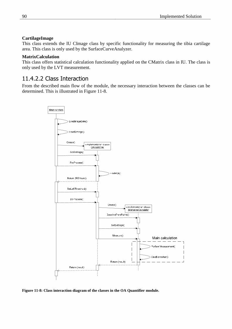
Implemented Solution
90
CartilageImage This class extends the IU CImage class by specific functionality for measuring the tibia cartilage area. This class is only used by the SurfaceCurveAnalyzer.
MatrixCalculation This class offers statistical calculation functionality applied on the CMatrix class in IU. The class is only used by the LVT measurement.
11.4.2.2 Class Interaction From the described main flow of the module, the necessary interaction between the classes can be determined. This is illustrated in Figure 11-8.
Figure 11-8: Class interaction diagram of the classes in the OA Quantifier module.

11.4 Module Design 91
The interaction diagram is limited to describe the interaction between the Main Function and the two main classes in the module only. This is done to give an overview of the process. For more details about the interaction between classes, the reader is referred to the source code included on the CD-ROM (see Appendix I). When the OAquantifier invokes the Measure method in the BiomarkerCalculator, the given measurement is performed. This task is described in detail in the following section.
11.4.3 User Settings
The user is able to select which measurement to perform. A set of general settings can be set and specific settings for each measurement. The following list states general and measurement specific settings:
Category User setting
General
Selection of measurement to perform.* Left offset Step size between measures
FI (none) LVT (none) CCV (none) CCS (none) SBV Optimal height of box*
Table 11-1: User settings in the OA Quantifier module. *These setting are available by dialog. All others by INI file.
For debugging both during the development of the module, but also if future users want to verify the methods, a set of debugging settings have been created:
Category Debug setting
General
True/false flag for indicating left offset ID of VIS measurement to use for indicating
FI
True/false flag for indicating the surface curve and Euclidean distance. ID of VIS measurement to use for indicating. True/false flag for debugging end point algorithm.
LVT
True/false flag for general debug of measurement. True/false flag for debugging the thickness measurement.
CCV True/false flag for general debug of measurement.
CCS True/false flag for general debug of measurement.
SBV True/false flag for general debug of measurement.
Table 11-2: Debug settings in the OA Quantifier module.
The approach of offering user settings in VIS is either by dialogs in the software or by external INI files. This standard is followed in the implementation of the OA Quantifier module. The two options are described in the following
11.4.3.1 Dialog Settings Settings, which are often used by the user, are available in the Segmentation dialog. Most of the user settings have been chosen to be available by dialog.

Implemented Solution
92
VIS offers to store given configurations set up by the user in the dialog. A VIS Configurations stores all specified Output Variables including settings of these. This functionality is used to set up three default configurations; one for each of the processing steps, which is step 2, 3 and 4 in the success scenario. The user then loads the Configuration for the given step and only changes settings if they differ from the standard.
11.4.3.2 INI files To offer the option of tuning the modules in VIS, Visiopharm uses INI files for a large number of settings. These settings are rarely set, and are for this reason put in INI files instead of creating dialogs with tons of settings. Settings from the INI files are loaded by the given module and applied by the given module. User settings not available by dialog are by INI files. In addition all debugging have been selected to be available in the INI files.
11.4.4 Error Handling
Errors are reported in VIS by using error codes. A set of general VIS error codes have been defined. Furthermore a set of specific error codes can be defined for each module individually. This has been done for the OA Quantifier module.
11.5 Performance
For evaluating the overall consumed time for the user to process a study, each part in the process has been time measured. The results are stated in Table 11-3. The process was performed at a 3.4GHz Intel Pentium with 1GB of RAM.

11.6 Conclusion 93
Time Step
Single[s] Batch
Manually defines individual base lines 5-7 20min
Manual setup of each Output value ~4 ~4s
An optimal value for the left offset <1 6min
Find optimal box height <1 6min
FI measurement <1
LVT measurement <1
CCV measurement <1
CCS measurement <1
SBV measurement <1
12min
Total 42 44min
Table 11-3: Consumed time of each step in the process. The total values include the specified setup time for eight Output variables. The batch job was performed on 201 specimens.
11.6 Conclusion
The required functionality was successfully implemented as a module in VIS. All required end points can be calculated by using the module. The measurements of the end points are performed in accordance with the measurement model using a base line and a left offset. The module was chosen to be available as an Output Variable in the Segmentation module. This was pointed out to be natural in the work flow of a pathologist, who is assessing mouse knee joints using VIS. In the implemented solution, the user is able to set up parameters for some of the end point measurements. This is easily performed by dialogs or by external INI files. This makes the solution user friendly. The optimal solution would be only one button to push and then results of all end point measures in return. This could not be complied with the implemented solution. Each end point must be set up and calculated individually. In addition a specific order is given for some of the end points, which requires parameters to be calculated in beforehand. All in all this gives a relative cumbersome workflow for the user. This is seen as a tradeoff of the advanced algorithms for the end points. A more simple approach would give a more simple implementation and thereby a more simple work flow. A requirement of as little work to be performed by the user as possible was stated. With the described solution, the user is required to perform manual corrections of the segmentation and manually define the base line of each specimen individually. Additionally, the above mentioned work with setting up the end point measurements and process of calculating them has to be done. This adds up to some work for the user, but less and more precise compared to manual assessment.

Implemented Solution
94
As stated in the requirements, the processing time is not critical, but has to be acceptable for the user. Tests have been performed and the time consumed by each step in the process is stated in section 11.5. The total process time is not seen as unacceptable for the user, nor are any of the process steps significantly more time consuming than others. For these reasons, no time was spent on optimization. All software guidelines stated in the requirements were successfully followed.

Chapter 12
Age Dependency Study
An age dependency study has been performed using the measurement methods described in Part II, and by calculation of the proposed end points. The developed OA Quantifier module described in Chapter 11 has been used to perform the measurements. The age dependency study is performed to illustrate the application of the proposed end points. In addition this study is a further validation of the end points, by comparing results with known OA age dependent tendencies. These tendencies are described in section 12.2. A visual inspection of the specimens in the study set has been performed in section 12.3 and evaluated with the known tendencies and results. In a larger perspective, an age dependency study gives the opportunity to investigate age related OA tendencies. In the human model of OA only non-invasive studies have been possible as described by Buckwalter et al. [3]. By the use of an animal model, more detailed information is possible to obtain. The performed age dependency study is on the frontier in the field of clinical OA research, by using the histological techniques, acquisition by microscope and advanced image analysis. The results may be an important component in the understanding of OA progression and in further research.
12.1 Study Set
The study set for the age dependency study, is similar to the study set applied for the histomorphometric analysis performed in this thesis (see section 2.1 for a detailed description). The study units are all male mice of strain STR/1N. The mice have been sacrificed with intervals of 3 weeks, giving groups at the ages of 6, 9, 12 and 15 weeks. Histological images of the medial part of the knee joints have been acquired by the procedure described in section 2.3, and referred to as specimens in the following. Only specimens with a valid medial tibia region are used in this study. The total numbers of specimens and valid specimens are stated by Table 12-1.
Definition: The time period between 6 weeks and 9 weeks are referred to as the first period , 9 to 12 the second period and 12 to 15 the third period .

Age Dependency Study
96
Time Mice Total Specimens
Specimens with Valid Tibia
6 weeks 24 123 96 9 weeks 24 121 96 12 weeks 24 119 94 15 weeks 22 124 89
Total 94 487 379
Table 12-1: Number of specimens, in the age dependency study set, grouped by time. The ‘Valid Tibia’ column states the numbers of specimens that have a valid tibia region for the study.
The specimens have been segmented using Visiopharm Auto Histology module as described in chapter 4.2. Manual corrections were performed subsequently of all four sets (4-5 hours/set of work), and base lines were pointed out using VIS Measurement tool.
12.2 Known Tendencies
A general set of known tendencies of OA impact in the knee joint, have been described throughout the thesis, mainly in Chapter 3. The age related tendencies, describes at what time each of the known tendencies occurs. This depends highly upon the applied animal model and even the given strain because each strain has its own age dependent properties of characterizing the OA progression. For the male mice of strain STR/1N, the biological changes, caused by OA development, are at the earliest observed around the age of fifty days (7 weeks), as stated by P. M. van der Kraan et al. [10]. At the age of twelve weeks, the OA impact tends to be severe for around 60% of the mice, according to U H Dietz et al. [7] and [18]. From these facts, it can be concluded that the studied period from six to fifteen weeks, includes the main period, of which STR/1N develops OA. It is a known fact that the chondrocytes are affected in advance of the cartilage matrix (Goldring [8]). Which degradation of either the cartilage matrix or the subchondral bone happens first, and eventual causes the other to happen, is unknown. The performed age dependency study might contribute to understanding of this. In the case of a study unit, with no basis for developing OA, none of the OA related symptoms are expected. In these cases, the chondrocytes maintain the cartilage matrix fully, and no decrease in the cellularity or degeneration of the cartilage matrix will occur. Neither does any thickening of the subchondral bone happen. By this general fact, any observed differences in the results can be seen as age related OA tendencies and not addressed any normal age related progress.

12.3 Observed Tendencies 97
12.3 Observed Tendencies
Each set of specimens has been inspected visually and described, to give a counterpart and add nuance to the results of the quantitative methods. The entire image of the histological section is evaluated for each specimen but the focus has mainly been kept at the tibia region.
6 Weeks The specimens are in general very healthy. No irregularities are seen in the surface of the cartilage matrix of any of the specimens. The cellularity is observed to be dense and uniformly distributed across the cartilage matrix. Large lacunae regions are spotted underneath the articular cartilage across the tibia region and only a low bone density is seen. For a few specimens, some of the bone tissue is torn apart, but this is addressed manual fumbling in the histology procedure.
9 Weeks These specimens are clearly affected by the disease. Irregularity and cavities are seen in the cartilage surface at the centre of the joint (the outermost right part in the image). The cartilage matrix is deformed at a minor scale, caused by pressure from the subchondral bone. The cellularity varies from high to medium in the right part of the cartilage whereas the left is in general high. The lacunae areas are smaller and more separated compared to the 6 weeks group. The subchondral bone enters from the right towards the left and splits the cartilage matrix and lacunae. For a few specimens, none of the above mentioned observations are done. They are in the same condition as the 6 weeks group.
12 Weeks The specimens of this group vary from almost none OA impact to highly affected. Degradation of the cartilage matrix is seen mainly in the joint centre, but also in the centre of the cartilage for some specimens. In a few cases, most of the right part of the cartilage matrix is missing. The cellularity is clearly reduced compared to the group of 6 weeks. This is general trend across the cartilage matrix i.e. difference between left and right are only seen for a few specimens. The condition of the subchondral bone and lacunae are identical to the 9 weeks group.
15 Weeks A few specimens are not noticeable affected by the OA disease, but the residual are highly affected. The cartilage matrix for the latter is missing in the right part and/or severe irregularity is seen in the surface. Still chondrocytes resides inside the remaining cartilage, but are clearly reduced compared to healthy cases. The condition of the subchondral bone are only slightly worse compared to the 9 and 12 weeks groups.
12.4 Performed Measurements
The performed measurements are based upon the described measurement model (see Chapter 5) and the best end points for each parameter of joint degradation (see Chapter 10) are measured and calculated as described in the following. For the measurement model, a left offset has been calculated for the entire age dependency study by guidelines described in section 5.2, and base lines have been pointed out manually.

Age Dependency Study
98
To measure the cartilage matrix, the LTV end point method has been performed, and the Fibrillation Index are calculated and used as reference. The cellularity has been measured by area fraction of chondrocyte tissue area divided by cartilage tissue area and both the average cellularity and the slope across the cartilage normalized by the average has been calculated and used as end points. The bone density has been measured by bone area fraction, and the average bone density has been calculated and used as end point.
12.5 Results
An optimal left offset was calculated to be oD=573px from occurrence of irregularity values of µD=1118px and σD=273px. The largest possible box height for measuring the bone density was found to be 423px. These setup values have been applied in the measurement process. The results have been grouped by time for each of the end points. Box plots for each group are seen in Figure 12-1. To quantify the OA progress in each period, the differences between each group of results have been calculated by an unpaired T-test and Mann-Whitney test, of which the p-values are stated in Table 12-2. The results are commented in the following. For the cartilage matrix end points, a drop in the FI and a rise in LTV values were expected. Both of these trend theses were fulfilled by the results. All of the tests for both end points indicated significant differences yet less significant for the second and third period. For the cellularity a decrease in the average value of the area fraction and larger negative values for the normalized slope of the area fraction were expected. Both of these trend theses were fulfilled but the trend thesis regarding the normalized slope was only weakly fulfilled. This indicates that the cellularity is affected uniformly across the cartilage matrix as the OA progresses over time. The decrease is strongest in the first period, and weaker for the last two periods. The subchondral bone develops rapidly, from having healthy symptoms with low bone density and large lacunae areas, to a strong OA impact indicated by thickening, in the first period. From the point of nine weeks, it stabilizes at a very unhealthy stage, with high bone density, throughout the rest of the observed period in this study.

12.5 Results 99
C
artil
age
Mat
rix e
nd p
oint
s
6 weeks 9 weeks 12 weeks 15 weeks
0
0.2
0.4
0.6
0.8
1F
ibril
latio
n In
dex
(FI)
Time 6 weeks 9 weeks 12 weeks 15 weeks
-4
-2
0
2
4
ln t
o tr
end
of s
ickn
ess
(LT
V)
Time (a) (b)
Cho
ndro
cyte
end
poi
nts
6 weeks 9 weeks 12 weeks 15 weeks0.01
0.02
0.03
0.04
0.05
0.06
0.07
0.08
Ave
rage
Cel
lula
rity
by A
rea
Fra
ctio
n
Time 6 weeks 9 weeks 12 weeks 15 weeks
-8
-6
-4
-2
0
2
4
6
8
x 10-3
Cel
lula
rity
by n
orm
aliz
ed S
lope
Time
(c) (d)
Sub
chon
dral
bon
e en
d po
ints
6 weeks 9 weeks 12 weeks 15 weeks
0.4
0.5
0.6
0.7
0.8
0.9
1
Bon
e V
olum
e [%
]
Time
(e)
Figure 12-1: Box plots of end point distributions by time. (a) Fibrillation Index. (b) Irregularity in cartilage matrix structure by LTV. (c) Cellularity by average area fraction. (d) Cellularity by normalized slope of area fraction. (e) Bone volume.

Age Dependency Study
100
Difference in mean
by T-test Difference in median by Mann-Whitney
1st period 2nd period 3rd period 1st period 2nd period 3rd period
Fibrillation Index <0.0001* 0.037 <0.0001 <0.0001 0.052 <0.0001
Irregularity by LTV <0.0001* 0.013 0.0006 <0.0001 0.0062 0.0007
Average cellularity <0.0001* 0.045 0.0006 <0.0001 0.012 0.0004
Cellularity by slope 0.0016* 0.20 0.28* <0.0001 0.11 0.11
Bone volume <0.0001 0.0075* 0.10 <0.0001 0.0055 0.17 *T-test has been performed for unequal distribution because of difference in variance indicated by f-tests rejecting the null-hypothesis at a 95% level of significance.
Table 12-2: P-values for both T-test and Mann-Whitney for consecutive groups by time for each of the end points.
12.6 Conclusion
The observed tendencies described in section 12.3 and the presented results corresponded well with each other, describing the OA age related tendencies in the study. These observations and results also correspond to the general known OA symptoms described in Chapter 3 and the age dependent tendencies of strain STR/1N described in section 12.2. Elaboration of the results is performed in the following to emphasize interesting and overall aspects of these results that are seen as new to the field. The end points were able to indicate the expected tendencies of the parameters of joint degradation related to age dependent development of OA. Only the cellularity by normalized slope yielded results with a low indication of the OA progress. This calculated feature is concluded to be a bad end point for age dependent tendencies. A clear trend was seen in that all parameters are affected the most in the first period. Especially thickening of the subchondral bone, progresses rapidly in the first period, more rapid than the two other parameters of joint degradation. This indicates that the bone is affected the first, and might be a great contribution to the degradation of the other parameters. This is a very interesting observation, which might contribute to the understanding of OA progression. The progress of both the degradation of the cartilage matrix and the decrease in cellularity is slower, but still describes the main part of period with OA impact. Because of this equality in progression, it is hard to determine which is affected first, and might cause or contribute to the affection of the other. This does not comply with the expected tendency of the cellularity being affected first, as described in section 12.2. Further study of the first period and the period until 6 weeks are required to clarify this. It is important to keep in mind that the concluded OA tendencies only can be applied to mice of strain STR/1N and not directly other animal models or in the case of human OA disease. For more general conclusions, further studies in other animal models are needed.

Part IV
Thesis Evaluation


Chapter 13
Discussion
The applied histomorphometric measurements and the proposed endpoints described in this report are generally discussed and put into a larger perspective in this chapter.
13.1 Measurement Method
13.1.1 Applied Model
In the work of this thesis a throughout examination has been performed using the applied measurement model. The model consists of two main components: a base line and a left offset. In the analysis of the histomorphometric methods and in the application of the end points, these components was found simple to use and yet worked as a good guideline. The base line helps to orient the measurement dependent on the orientation of the articular cartilage and thereby makes the measurements consistent.
13.1.2 Sampling
In the performed measurements, the possibility of sampling across the tibia region was used to determine possible features for end points. This resulted in the discovery of a strong end point of cellularity by normalized slope in the area fraction measurements. A general technique of using the difference between the left and right side of the medial tibia for determining the stage of OA affection was also found by the sampling process. Additional strong end points can be found by taking advantage of this difference by an asymmetry model. This is addressed further in section 14.1.2.
13.2 End Points
A demand of strong quantitative end points was stated in the motivation of this thesis (see section 1.4) and additionally addressed in the evaluation of current histological assessment (see Chapter 3). Strong end points have been defined for each of the parameters of joint degradation and application of these has been illustrated by significant indication of treatment effect and by performing an age dependent study.

Discussion
104
The important factor is the correctness of the end points and an argumentation of this has been performed for each end point in the discussion section of the three measurement chapters (see sections 7.4, 8.4, 9.4). By visually evaluating the specimens, the irregularities in the cartilage surface are clearly seen. The calculated cartilage matrix features were able to find these irregularities. It is far harder to assess the cellularity and subchondral bone manually. The cellularity is rather diffuse and when evaluating it, it is almost only possible to make a distinction between few chondrocytes and many. Everything in between is impossible to evaluate manually, which is confirmed by the manually given pathology scores that only makes use of three out of five possible scores and with most observations in the middle group (score 2). Same tendency is seen when evaluating the subchondral bone. It is only possible to distinguish between a bone containing a high number of large lacunae and a low number of small lacunae, and everything in between is difficult to evaluate and the score 3 is given. The discussion in the paragraph above emphasizes the difficulties of manually distinguishing between the grades of disease affection. The proposed end point indicates strong differences between extreme groups of specimens grouped by manually given pathology scores and at the same time an overall trend is confirmed, which indicates that higher precision is possible with these quantitative measurements compared to the manual ranking system. By the use of the proposed end points the above mentioned difficulties are avoided. In addition, errors in the manual given score for the study set used for the histomorphometric analysis was found by the applied and points (see Appendix B). This was pointed out at the meeting the March 30, 2006 (see Appendix D), and the errors were subsequently corrected. This is a good example of quantitative methods being superior to manual assessment.

Chapter 14
Future Work
The work of this thesis is a good basis for determining strong quantitative end points for the mouse model of OA, still more work has to be done. Possible improvements and new studies is addressed in this chapter inspired by observations and gained experience in the work of this thesis.
14.1 Measurement Model
14.1.1 Simplification of Left Offset
Evaluation of the left offset indicated that this component is important, but the precision of the applied value is not crucial. For this reason a more simple approach or a rule of thumb is suggested to define a proper left offset. From the gained experience in the work of this thesis, the following approach is suggested:
• Measure the length across all cartilage matrixes in the study set. The left offset is defined by the longest divided by three.
A study of this approach has to be carried out to evaluate the correctness.
14.1.2 Asymmetry model
From observations and by known tendencies described by Meacock [16] the right side of the tibia is affected more and in advance of the left side. This results in an asymmetry of the two areas that could be the basis of a strong measurement model. The degree of sickness caused by OA can be determined by performing calculations of end points inside two boxes in each side and measure the difference (see Figure 14-1). This approach is less cumbersome compared to sampling and calculation of slope, but may reveal the same results.

Future Work
106
Figure 14-1: Asymmetry model illustrated by pairs of boxes on specimen 103-14. 'A' boxes are for measurements of cartilage matrix and cellularity. 'B' boxes are for measurements of subchondral bone.
14.2 End Points
14.2.1 Further Validation
To fully validate the proposed end points, study of the application on a larger scale is required. In addition, research of application of the end points in other animal models of OA, e.g. rabbits or guinea pigs, is of great interest and would further validate the end points.
14.2.2 New Approaches
The thickening of the subchondral bone is mainly seen as a v-shaped entering from the joint centre (right side of the specimen images). The lacunae blobs in the subchondral region are large and connected in the case of a healthy specimen and smaller and separated in the case of OA affected. A more sophisticated feature based upon the above described observations of the subchondral composition, is a possible end point for the condition of the subchondral bone. The idea occurred at a late stage of the thesis and no study of this has been performed, but is suggested for future research in the field.
14.3 Functionality Improvements
14.3.1 Base Line
The base line is essential in the applied measurement model. In the work of this thesis, the base line has been pointed out manually. The base line might be found automatically by fitting a line through
A2
B2
A1
B1

14.3 Functionality Improvements 107
the cartilage/bone interface from measurements of the segmented tissue in this area. An implementation of this and a validation study is proposed as possible future work.
14.3.2 Focus of Measurement
To ensure correct and optimal end points it is important that the focus of the end points measurements are kept on the most affected area. This is the key idea of the proposed measurement model in this thesis but still by the used approach of segmentation of the image, the focus partly relies on manual corrections. Improvements of the segmentation and measurement methods are recommended to guarantee that the affected area is inside without any need of manual corrections. In addition, bone area in the area towards the joint centre (right side of specimens) could be interesting to include in the measurements. The density and composition of this bone area is observed related to the level of OA impact.

Future Work
108

Chapter 15
Conclusion
The overall objective of this thesis was to clarify and propose strong quantitative histomorphometric measurements related to the stage of OA affection in the mouse model. The scope has been of the medial tibia region of the knee joint and parameters of joint degradation caused by OA. A set of quantitative measurements have been described and proposed from the knowledge of histopathology assessment. The measurements are performed according to a proposed measurement model using a base line and a left offset to keep focus on the most affected area of the joint. The measurement model was concluded to be a good foundation for the measurements, but the precision of the applied left offset was found less important. The measurements were performed using image analysis of microscope images of histopathological sections of knee joints from mice. The images were from a study set of fifty mice. As part of the image analysis, segmentation of the images was performed using the Visiopharm Auto Histology module. The segmentation process was successful and the segmentation required a limited work of manual corrections. The specific measurements were carried out by geometric calculations and algorithms implemented in C++ using Visiopharm Imaging Utilities SDK. For the parameter of the cartilage matrix structure, a measurement of the cartilage thickness was used to measure irregularities in the cartilage surface caused by OA impact. An end point was calculated by a statistical feature of this measurement. This end point was found to have a strong correlation with the manually given pathology score, which is interpreted as the stage of OA affection. By argumentation in section 3.3 the cellularity was defined by a fraction of chondrocyte area divided by cartilage area. By sampling across the tibia articular cartilage, a feature was calculated by the slope of cellularity measurements. This feature was found to be a strong end point for the cellularity by a high correlation with the manually given pathology score. The condition of the subchondral bone has been assessed by the bone density defined by a fraction of measured bone tissue divided by measured area underneath the articular cartilage. This feature has been proven applicable in the model of guinea pigs by Pastoureau et al. [20] and was found in this thesis to be the best end point for the subchondral bone in the mouse model. The end point had a strong correlation with the manually given pathology score.

Conclusion
110
All three end points were applied to measure the effect of a drug compound applied to half of the study set. All end points indicated highly significant effect of the applied drug by both unpaired Students T-test and Mann-Whitney. This validated the end points even further. The application of the end points has been illustrated by an implementation in a Visiopharm VIS module. The module was used to perform an age dependency study. The end points complied with the known age dependent trends. In addition, the study has clarified a trend of the thickening process of the subchondral bone occurs in advance of both the cartilage matrix and the cellularity of chondrocytes being affected, in the mouse model of OA. An asymmetry of the left and right side of the medial tibia was found in this work. A clear correlation was found between the progress of OA and the asymmetry. This correlation indicates that the right side of the medial tibia is degenerated first, and then the affection of OA evolves towards the left side, which confirms the work performed in the guinea pig model of OA by [20]. The tendencies pointed out are only confirmed in this study of OA in the mouse model, and cannot necessary be mapped to other animal models or for human diagnostics. Further study of other animal models has to be performed. As an overall result of this thesis, a set of strong quantitative histomorphometric end points have been defined. In perspective these end points can be an important component in the development of an international standard of assessing the degree of osteoarthritis.

List of Figures
Figure 2-2: A frontal image of the medial part of specimen 103-17 with labels for the different types of area. Areas of articular cartilage and meniscus have been enhanced by outlining in this illustration. ................................ 15
Figure 3-2: Specimen 196-14. Measuring FI by the Euclidean distance and the surface curve, both indicated by black lines. ............................................................................................................................................................. 20
Figure 3-3: First approach of cartilage matrix thickness measurement. The cartilage surface and cartilage/bone interface are measured separately from a horizontal line. Specimen 133-11. ............................................................. 20
Figure 3-4: Final approach of measuring cartilage matrix thickness. A line is fitted trough the cartilage/bone interface. Thickness are measured perpendicular to this line. Specimen 362-14. ........................................................ 21
Figure 3-6: Binary indication of bone density measurement. Black area is measured as bone, white as not-bone. Residual area is excluded from measurement. Specimen 133-5. ................................................................ 23
Figure 4-2: Defined mask and labels for segmentation. ................................................................................................... 28
Figure 4-3: Segmentation result of specimen 103-14. (a) Original image. (b) Segmented image.................................... 28
Figure 5-1: Medial image of specimen 103-14 with Region of Interest (ROI) indicated................................................. 32
Figure 5-2: Measurements for specimen 133-5 using left side of mask as reference. (a) Result of irregularity measurement of the cartilage surface, (b) the first numerical derivative of the thickness measurement..... 33
Figure 5-3: Cusum method applied by using a V-mask. The origin of the V-mask is indicated by the first point where the process is out of control by violating the upper arm. The raw data are only generated to illustrate an example. ....................................................................................................................................................... 35
Figure 5-4: Plot of irregularity occurrences found by using left side of mask as reference. The histogram indicates the distribution of the occurrences. Measured cartilage curves are guidelines. ................................................. 37
Figure 5-5: Plot of irregularity occurrences found by using left cartilage rounding as reference. The histogram indicates the distribution of the occurrences. Measured cartilage curves are guidelines............................................. 37
Figure 7-1: Specimen 196-14. Measuring delimited FI by the Euclidean distance and the surface curve, both indicated by jagged black lines. ...................................................................................................................................48
Figure 7-2: Thickness measurement illustrated on segmented image of specimen 103-17. Used interval of measurements for this illustration is 60px. .......................................................................................................................... 49
Figure 7-4: Ambiguous thickness measurement definitions. Base line and thickness measurement indicated on a cropped part of specimen 213-5. (a) To the exact surface (applied in this thesis). (b) Sum of cartilage tissue. (c) Following inner curvature....................................................................................................................... 50
Figure 7-5: Theses for thickness measurement results X of two extremes. (a) Healthy specimen. (b) Specimen highly affected by OA. ............................................................................................................................................ 50
Figure 7-6: Results of three handpicked measurements. (a) Thickness measurement. (b) Trend variance of measurement (last 25 samples of each measurement have been excluded as explained). .................................................. 52
Figure 7-7: Basic statistics for the trend variance. Results are grouped by manually given pathology score. ................. 53

List of Figures
112
Figure 7-8: Transformation by using ln to approximate normal distribution. (a) Trend variance. (b) ln to the trend variance (LTV)............................................................................................................................................. 54
Figure 7-9: Box plots of calculated matrix features. (a) FI. (b) Overall variance. (c) Slope. (d) LTV........................... 54
Figure 7-10: Box plots of calculated cellularity features grouped by control and treated specimens. (a) FI. (b) Overall variance. (c) Slope. (d) LTV. ....................................................................................................................... 56
Figure 8-1: Cellularity measurement with an interval of 10px illustrated on segmented image of specimen 137-20. (a) Overview with base line and left offset indicated. (b) Detailed view of base line and perpendicular sample lines. ............................................................................................................................................................. 59
Figure 8-2: Expected trends of measurement results for Y. (a) Healthy. (b) Medium affected. (c) Sick. ...................... 60
Figure 8-4: Measured cartilage area for selected specimens. ........................................................................................... 62
Figure 8-5: Measured chondrocyte area for selected specimens. (a) Specimen 262-11, score 0. (b) Specimen 133-5, score 2. (c) Specimen 760-14, score 5.......................................................................................................... 63
Figure 8-6: Cellularity by area fraction ρarea for a selected specimen. (a) Original measurement. (b) Smoothed measurement to ease interpretation of measurement. A kernel size of 30 samples has been applied. ......... 63
Figure 8-7: Spike problem illustrated by last 50 samples of all chondrocyte area fraction calculations. Exclusion of last 15 samples is illustrated by a vertical red dotted line................................................................................... 64
Figure 8-8: Box plots of calculated cellularity features. (a) Overall average. (b) Normalized slope. (c) By threshold.... 64
Figure 8-9: Box plots of calculated cellularity features grouped by control and treated specimens. (a) Overall average. (b) Normalized slope. (c) By threshold. ....................................................................................................... 66
Figure 9-1: Performing subchondral bone measurement on segmented image of specimen 174-14. Base line and left offset from the measurement model is indicated. #1 Top offset. #2 fixed box height. ................................ 70
Figure 9-2: Bone density measurements. (a) Specimen 174-17, score 0. (b) Specimen 862-20, score 8 ......................... 71
Figure 9-3: Box plots of measured subchondral bone features grouped by manually given pathology score. (a) Average bone density. (b) Slope of bone density. ...................................................................................................... 71
Figure 9-4: Box plots of measured subchondral bone features grouped by control and treated. (a) Average bone density. (b) Slope of bone density. ............................................................................................................................ 73
Figure 10-1: Pairwise scatterplots of the end points. (a) Cartilage and cellularity. (b) Cartilage and bone. (c) Cellularity and bone. ...................................................................................................................................................... 77
Figure 11-2: Screenshot from running VIS software using the Segmentation module. The following areas are indicated on the screenshot: (1) Module bar. (2) Toolbar. (3) Work area. (4) Card view of study in VIS database... 83
Figure 11-3: Base line pointed out manually by using measurement tool in VIS. The VIS measurement tool is the black line across the image. ...................................................................................................................................86
Figure 11-4: Steps for adding and setting up an Output Variable in VIS. In this example the Output Variable is an OA measure of the chondrocyte cellularity, which is calculated by the OA Quantifier module. ....................... 87
Figure 11-5: Performing calculation of Output Variables in the Segmentation module in VIS. In this example only one OA measure has been added for calculation. (a) The Calculate button is pressed to initiate the calculation. (b) The result is seen in the column next to the given calculation................................................................ 87
Figure 11-7: Class diagram of the calculation functionality classes in the OA Quantifier module.................................. 89
Figure 11-8: Class interaction diagram of the classes in the OA Quantifier module........................................................ 90
Figure 12-1: Box plots of end point distributions by time. (a) Fibrillation Index. (b) Irregularity in cartilage matrix structure by LTV. (c) Cellularity by average area fraction. (d) Cellularity by normalized slope of area fraction. (e) Bone volume............................................................................................................................. 99
Figure 14-1: Asymmetry model illustrated by pairs of boxes on specimen 103-14. 'A' boxes are for measurements of cartilage matrix and cellularity. 'B' boxes are for measurements of subchondral bone. ............................. 106

14.3 Functionality Improvements 113
Figure 2 – Standard deviation of first numerical derivate of the curvature measurement with calculation of distance D illustrated.................................................................................................................................................... 133
Figure 3 - Medial Measurement image, with region of interest indicated. ..................................................................... 134
Figure 15-1: Segmentation result of specimen 103-14. (a) Original image. (b) Segmented image................................ 139
Figure 15-2: Classifier uses too narrow range, which results in wrong segmentation. (a) Specimen 174-14 (b) Specimen 262-11. ....................................................................................................................................................... 140
Figure 15-3: Specimen 931-14. An example of good segmentation. Two overlapping chondrocytes are identified seperately, illustrated (a) before and (b) after segmentation. ..................................................................... 141
Figure 15-4: Specimen 133-5. Missing segmentation of a chondrocyte......................................................................... 141
Figure 15-5: Specimen 789-14. Misclassification of cartilage border leads to a series of incorrect chondrocyte centers, illustrated (a) before and (b) after segmentation. ....................................................................................... 141
Figure 15-6: Specimen 216-11. Vague chondrocyte leads to several chondrocyte centers, illustrated (a) before and (b) after segmentation. ..................................................................................................................................... 141
Figure 15-7: Lacunae nucleus tissue misclassified wrong in two cases: (a) Specimen 931-17, as cell tissue. (b) Specimen 985-11, as lacunae background. ................................................................................................................. 142
Figure 15-8: Specimen 862-17. Lacunae incorrect segmented as cell tissue. Illustrated (a) before and (b) after segmentation. ............................................................................................................................................. 142
Figure 15-9: Specimen 862-14. Lacunae incorrect segmented as cartilage tissue. Illustrated (a) before and (b) after segmentation. ............................................................................................................................................. 142
Figure 15-10: Examples of special cases of identification of the tibia cartilage region. Cropped images are taken from following specimens: (a) 133-11 (b) 216-8 (c) 137-20 (d) 213-2 (e) 174-20............................................. 143

List of Figures
114
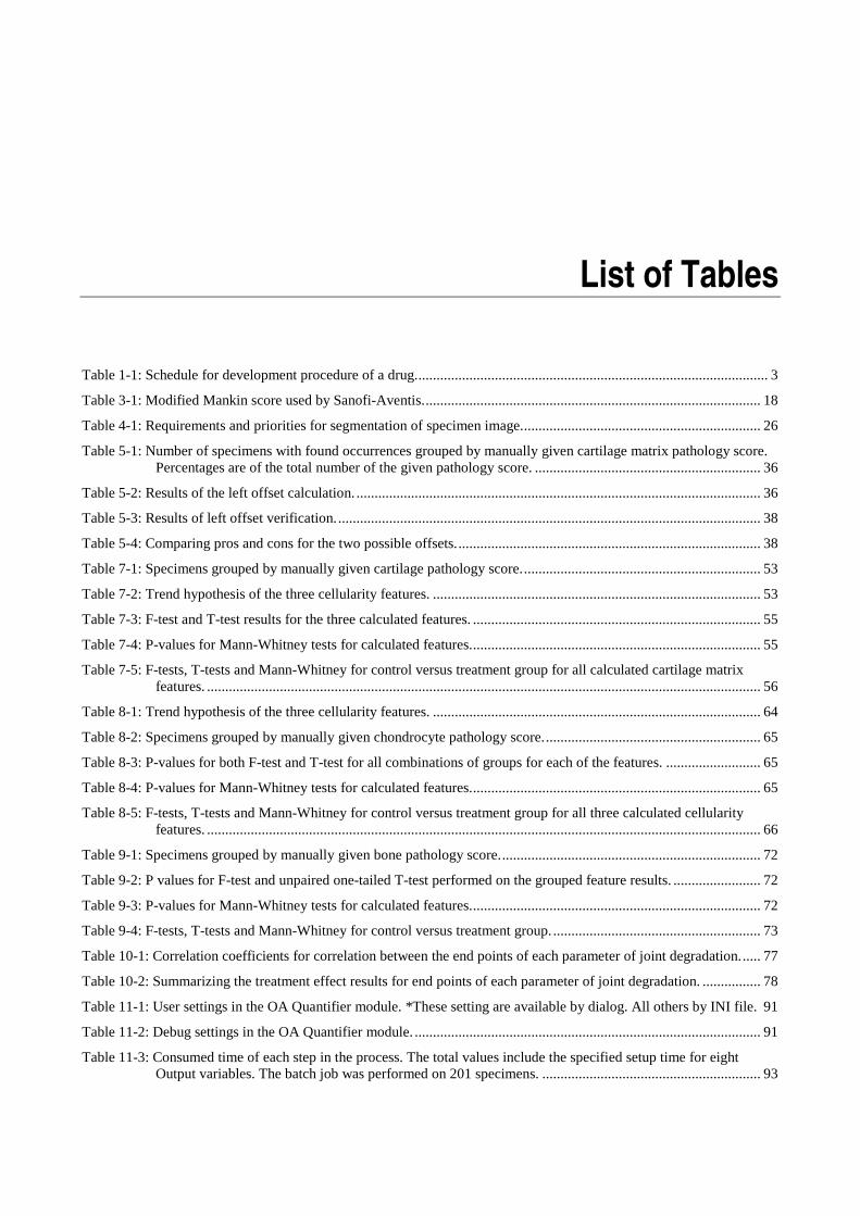
List of Tables
Table 1-1: Schedule for development procedure of a drug................................................................................................. 3
Table 3-1: Modified Mankin score used by Sanofi-Aventis............................................................................................. 18
Table 4-1: Requirements and priorities for segmentation of specimen image.................................................................. 26
Table 5-1: Number of specimens with found occurrences grouped by manually given cartilage matrix pathology score. Percentages are of the total number of the given pathology score. .............................................................. 36
Table 5-2: Results of the left offset calculation................................................................................................................ 36
Table 5-3: Results of left offset verification..................................................................................................................... 38
Table 5-4: Comparing pros and cons for the two possible offsets.................................................................................... 38
Table 7-1: Specimens grouped by manually given cartilage pathology score.................................................................. 53
Table 7-2: Trend hypothesis of the three cellularity features. .......................................................................................... 53
Table 7-3: F-test and T-test results for the three calculated features. ............................................................................... 55
Table 7-4: P-values for Mann-Whitney tests for calculated features................................................................................ 55
Table 7-5: F-tests, T-tests and Mann-Whitney for control versus treatment group for all calculated cartilage matrix features. ........................................................................................................................................................ 56
Table 8-1: Trend hypothesis of the three cellularity features. .......................................................................................... 64
Table 8-2: Specimens grouped by manually given chondrocyte pathology score............................................................ 65
Table 8-3: P-values for both F-test and T-test for all combinations of groups for each of the features. .......................... 65
Table 8-4: P-values for Mann-Whitney tests for calculated features................................................................................ 65
Table 8-5: F-tests, T-tests and Mann-Whitney for control versus treatment group for all three calculated cellularity features. ........................................................................................................................................................ 66
Table 9-1: Specimens grouped by manually given bone pathology score........................................................................ 72
Table 9-2: P values for F-test and unpaired one-tailed T-test performed on the grouped feature results. ........................ 72
Table 9-3: P-values for Mann-Whitney tests for calculated features................................................................................ 72
Table 9-4: F-tests, T-tests and Mann-Whitney for control versus treatment group.......................................................... 73
Table 10-1: Correlation coefficients for correlation between the end points of each parameter of joint degradation...... 77
Table 10-2: Summarizing the treatment effect results for end points of each parameter of joint degradation. ................ 78
Table 11-1: User settings in the OA Quantifier module. *These setting are available by dialog. All others by INI file. 91
Table 11-2: Debug settings in the OA Quantifier module. ............................................................................................... 91
Table 11-3: Consumed time of each step in the process. The total values include the specified setup time for eight Output variables. The batch job was performed on 201 specimens. ............................................................ 93

List of Tables
116
Table 12-1: Number of specimens, in the age dependency study set, grouped by time. The ‘Valid Tibia’ column states the numbers of specimens that have a valid tibia region for the study. ........................................................ 96
Table 12-2: P-values for both T-test and Mann-Whitney for consecutive groups by time for each of the end points. .. 100
Table 15-1: Results of evaluation of counting chondrocytes. *These results are in number of chondrocytes. **This t-test rejects the null-hypothesis on a 95% level of significance......................................................................... 139
Table 15-2: Summery of results from evaluation of segmentation by VIS Auto Histology module. ............................. 140

Bibliography
[1] Arthritis Foundation. http://www.arthritis.org
[2] Alliance Pharmaceutical Corp, Phases of Product Development. 02, 2006. http://www.allp.com/drug_dev.htm
[3] Buckwalter JA, Mankin HJ. Articular cartilage: degeneration and osteoarthritis, repair, regeneration, and transplantation. Instr Course Lect. 1998;47:487-504.
[4] J. M. Carstensen. Image analysis, Vision and Computer Graphics 2nd ed., Technical University of Denmark, 2002.
[5] Castleman, K.R., Digital Image Processing. 2nd ed. 1996, Englewood Cliffs, New Jersey: Prentice-Hall
[6] Delesse, M.A., Procédé mécanique pour déterminer la composition des roches. Compte-Rendus d' Académie des Sciences, Paris, 1847;25;544-545.
[7] UH Dietz, K Rudolphi, N Gerwin. Three Animal Models of Osteoarthritis are Characterized by Similar Disease Marker Expression Patterns Despite Different Disease Etiology, Osteoarthritis and Cartilage;2004
[8] Goldring MB. The role of the chondrocyte in osteoarthritis [review]. Arthritis Rheum 2000;43:1916–26.
[9] H. J. Helminen, A.-M. Säämänen, H. Salminen, M. M. Hyttinen. Transgenic mouse models for studying the role of cartilage macromolecules in osteoarthritis. Rheumatology 2002; 41: 848-856.
[10] P. van der Kraan, Alwin Scharstuhl, Henk M van Beuningen, Elly L Vitters, Wim B van den Berg Nijmegen. Increased Expression of Bone Morphometric Protein-2 and -4 in Osteoarthritis lesions of STR/1N mice, Arthritis & Rheumatism;2001
[11] Craig Larman; Applying UML and Patterns 2nd Edition; Prentice Hall PTR 2002
[12] Stan Z. Li. Markov random field modeling in image analysis. Springer-Verlag New York. 2001

Bibliography
118
[13] Lægemiddelstyrelsen Godkendelse af lægemidler. 02, 2006. http://www.laegemiddelstyrelsen.dk/1024/visLSArtikel.asp?artikelID=665
[14] OARSI, OsteoArthritis Research Society International. www.oarsi.org
[15] Mankin HJ, Dorfman H, Lippiello L, Zarins A. Biochemical and metabolic abnormalities in articular cartilage from osteoarthritic human hips. II. Correlation of morphology with biochemical and metabolic data. J Bone Joint Surg Am, Apr;53(3):523-37, 1971.
[16] Meacock SCR, Bodmer JL, Billingham MEJ. Experimental; Osteoarthritis in guinea pigs. J Exp Pathol; 1990;71:279–93.
[17] Miller and Freund’s, Probability and Statistics for Engineers 6th Edition; Prentice Hall; 2000
[18] Mouse Genome Database (MGD), Mouse Genome Informatics Web Site, The Jackson Laboratory, Bar Harbor, Maine. World Wide Web (URL: http://www.informatics.jax.org). Inbred Strains of Mice: STR (07, 2006). http://www.informatics.jax.org/external/festing/mouse/docs/STR.shtml
[19] Page ES. Continous inspection schemes. Biometrika vol. 41; 1954; 100-115.
[20] P. Pastoureau, Leduc S, Chomel A, De Ceuninck F. Quantitative assessment of articular cartilage and subchondral bone histology in the meniscectomized guinea pig model of osteoarthritis. Osteoarthritis and Cartilage, Jun;11(6):412-23, 2003.
[21] Pritzker KP, Gay S, Jimenez SA, Ostergaard K, Pelletier JP, Revell PA, Salter D, van den Berg WBP. Osteoarthritis cartilage histopathology: grading and staging. Osteoarthritis and Cartilage, Jan;14(1):13-29, 2006.
[22] William C. Shiel Jr., MD, FACP, FACR Osteoarthritis; http://www.medicinenet.com/osteoarthritis/article.htm
[23] Van der Sluijs JA, Geesink RG, van der Linden AJ, Bulstra SK, Kuyer R, Drukker J. The reliability of the Mankin score for osteoarthritis. J Orthop Res, Jan;10(1):58–61, 1992.
[24] Stephen B. Vardeman; AICE Short Course on "Advanced SPC"; Cusum charts; 2001
[25] Visiopharm; The Visiopharm Integrator System http://www.visiopharm.com/pdf/vis_web.pdf*
[26] Visiopharm and Aventis, A new quantitative method for the measurement of gross morphological changes in the animal models of osteoarthritis.; www.visiopharm.dk; 2003*
[27] Visiopharm and Aventis, A new quantitative method for the measurement of subchondral bone changes in animal models of osteoarthritis.; www.visiopharm.dk; 2003*
[28] Visiopharm and Aventis, Automated histomorphometric analysis of joint damage in a mouse model of osteoarthritis.”, www.visiopharm.dk; 2004*

14.3 Functionality Improvements 119
[29] Visiopharm and Aventis, Automated Histomorphometry, System description and configuration, 2004*
[30] Wicksell, S.D., The corpuscle problem. A mathematical study of a biometric problem. Biometrika 1925;17;84-99.
[31] K. Østergård Fakta om slidgigt – et overblik; 02, 2006. http://www.slidgigt.dk/Fakta/default.aspx
*These documents have been included on the CD-ROM. See Appendix I.

Bibliography
120

Appendix A
List of Control and Treated Groups
The following is a list indicating the grouping into control and treatment group of the specimens in study STR/1N-25-05 by Sanofi-Aventis. The specified number is the study unit number of the given mouse.
Control Treated 103 174 133 213 137 296 196 351 216 354 262 372 317 377 362 405 376 439 397 536 398 568 476 605 489 609 497 723 502 782 602 789 631 800 735 801 760 821 816 824 820 843 822 845 832 890 862 931 921 985

List of Control and Treated Groups
122

Appendix B
Manually Given Pathology Score
The following is a list of manually given pathology scores for the specimens in study STR/1N-25-05 by Sanofi-Aventis. The list was updated in April 2006 because of incorrect given pathology scores. The errors was found in the initial analysis by the use of the proposed methods, and pointed out at the meeting with H. Gühring March 31, 2006, see Appendix D. Corrected scores are emphasized in bold.
Modified Mankin score used by Sanofi-Aventis
The pathology scores in the list are from the scoring table below.
Cartilage matrix structure
Cellularity of chondrocytes
Subchondral bone
0 Normal 0 Normal 0 Normal
1 Surface irregularities
2 Reduced 3 Remodeling processes
3 Superficial fibrillation
5 Strongly reduced 8 Thickening
6 Clefts in deep zones
8 Total loss of cartilage
8 Complete loss of cartilage

Manually Given Pathology Score
124
Study Unit Measurement Cart Cell Bone
Study Unit Measurement Cart Cell Bone
103 11med-F 568 11med 1 2 3 103 14med 3 2 3 568 14med 1 2 3 103 17med 3 2 3 568 5med 1 2 8 103 20med 6 2 8 568 8med 1 2 8 103 23med-T 8 2 8 602 11med 1 2 3 133 11med 8 2 8 602 14med 6 2 8 133 14med 6 2 8 602 17med 1 2 8 133 17med-F 602 8med 1 2 3 133 5med-T 6 2 8 605 10med 1 2 3 133 8med 6 5 8 605 14med 1 2 3 137 11med 1 2 8 605 17med 3 2 3 137 14med 3 2 8 605 20med-T 1 0 3 137 17med 6 2 8 605 7med-F 137 20med 6 5 8 609 11med 3 2 8 174 11med-F 609 14med 8 5 8 174 14med 1 2 8 609 17med 6 5 8 174 17med 1 2 3 609 8med 3 2 8 174 20med-T 0 2 3 631 11med 8 5 3 174 23med-T 1 2 3 631 14med 8 5 3 174 8med-F 631 17med 8 5 8 196 11med 8 5 8 631 20med 6 2 3 196 14med 8 5 8 723 11med 6 2 8 196 17med 6 5 8 723 14med 6 5 8 196 8med 6 5 8 723 17med 8 2 3 213 11med 3 2 8 723 20med 6 2 3 213 2med-F 735 11med 3 2 3 213 2med-T 6 2 8 735 14med 6 2 8 213 5med 6 2 8 735 17med 6 5 8 213 8med 6 2 8 735 20med 6 2 8 216 11med 3 2 8 760 11med 8 5 8 216 14med 6 2 8 760 14med 8 5 8 216 17med-T 6 5 8 760 17med 8 5 8 216 5med-F 760 20med-T 6 5 8 216 8med 3 2 8 760 8med-F 262 11med 1 0 3 782 11med 3 2 3 262 14med 1 2 3 782 14med 6 2 3 262 17med-T 0 2 782 17med 1 2 3 262 5med-F 3 782 20med-T 3 2 3 262 8med 1 2 3 782 8med-F 296 11med 8 5 8 789 11med 3 2 8 296 14med 8 5 8 789 14med 6 2 3 296 17med 8 5 8 789 17med 3 2 8 296 20med-T 8 5 8 789 20med-T 3 2 3 296 8med-F 789 8med-F 317 11med 8 2 8 800 13med 1 2 3 317 14med 8 2 8 800 17med 1 2 3 317 17med 8 2 8 800 20med 1 2 3 317 20med 6 2 8 800 23med 0 0 3 351 11med 3 2 8 801 11med 6 5 8 351 14med 6 2 8 801 14med 6 2 3 351 17med-T 3 2 8 801 17med 6 2 3 351 5med-F 801 20med 1 2 3 351 8med 3 2 8 801 23med 354 11med 8 2 8 816 11med 1 2 8 354 14med 8 2 3 816 14med-T 3 5 3 354 17med-F 816 17med-T 3 2 3 354 5med-T 6 2 3 816 2med-F 354 8med 8 5 8 816 5med-F 362 11med 6 2 8 816 8med 1 0 3 362 14med 6 2 8 820 11med 6 2 8 362 17med 6 2 8 820 14med 6 2 3 362 20med-F 820 17med 3 5 3 362 7med-T 3 2 8 820 8med 6 5 8

14.3 Functionality Improvements 125
Study
Unit Measurement Cart Cell Bone Study
Unit Measurement Cart Cell Bone 372 11med-T 8 2 8 821 11med-F 372 14med-F 821 14med 8 2 8 372 14med-T 8 2 8 821 17med 8 2 8 372 17med 8 2 8 821 20med 8 2 8 372 20med 8 2 8 821 23med-T 8 2 3 372 23med-F 822 10med-F 376 14med 6 2 8 822 13med 1 2 8 376 17med 6 5 3 822 17med 3 2 8 376 20med 6 2 8 822 20med 3 2 8 376 23med 6 5 3 822 23med-T 3 2 377 11med 1 2 3 824 10med 1 2 8 377 14med-F 824 14med 0 2 3 377 2med-T 3 2 3 824 17med 0 2 3 377 5med 1 2 3 824 7med 1 2 8 377 8med 1 2 3 832 11med 8 2 3 397 11med 6 2 3 832 14med 3 5 3 397 14med 6 2 3 832 17med-T 3 2 3 397 5med 3 2 8 832 5med-F 397 8med 3 2 8 832 8med 6 2 8 398 13med 8 2 8 843 11med 8 2 8 398 17med 6 5 3 843 14med-T 6 2 3 398 20med 6 5 3 843 17med-T 1 2 0 398 23med 6 5 3 843 2med-F 405 10med 1 0 8 843 5med-F 405 14med 3 2 8 843 8med 8 2 8 405 17med 6 5 8 845 11med 3 2 8 405 20med-T 3 2 3 845 14med 1 2 3 405 7med-F 845 17med 6 2 3 439 10med 1 2 8 845 21med 1 0 3 439 14med 3 2 3 862 14med 8 2 8 439 17med 3 2 3 862 17med 8 2 8 439 20med 1 2 3 862 20med 6 5 8 476 11med 1 0 3 862 23med 6 2 8 476 14med 1 2 3 890 11med 1 0 3 476 17med 3 5 3 890 14med 0 2 3 476 20med-T 0 2 3 890 17med 0 2 8 476 7med-F 890 20med 1 2 3 489 11med 6 2 8 921 11med 1 2 3 489 14med 6 2 8 921 14med 1 2 3 489 17med 6 2 3 921 17med 0 2 0 489 20med-F 921 8med 1 2 3 489 8med-T 6 5 8 931 11med 3 2 8 497 10med-F 931 14med 6 5 8 497 14med 1 2 3 931 17med 6 2 8 497 17med 3 2 3 931 20med 3 2 3 497 20med 3 2 8 985 11med 1 2 3 497 23med-T 3 2 3 985 14med 0 2 3 502 14med 6 2 8 985 17med 1 2 3 502 17med 6 2 8 985 8med 1 2 3 502 20med 8 2 8 502 23med 6 2 3 536 10med-F 536 14med 3 2 3 536 17med 6 5 3 536 20med 3 5 3 536 23med-T 1 2 3

Manually Given Pathology Score
126

Appendix C
First Presentation for BE and MGR
Thursday the 28th of March 2006. Participants: Michael Grunkin (Visiopharm), Bjarne Ersbøll (IMM, DTU), Eigil Mølvig Jensen (stud. M.Sc. at DTU).
Agenda
1. EMJ makes a presentation of preliminary results and used methods. 2. All discuss further improvements and overall goal for project.
Summery of EMJs presentation
1. Segmentation has been performed using module develop by Thomas Ebstrup. Segmentation results were overall a success.
2. Methods for measuring the condition of the cartilage matrix structure, cellularity of Chondrocytes and bone density were presented. In general for all the applied methods a polynomial fitted through the cartilage/bone interface was used. Measurements were performed perpendicular from this line in a fixed number of slices.
3. Cartilage matrix structure has been measured by Fibrillation Index (FI), Fibrillation Area Index (FAI) and irregularity in thickness. The results are as follows:
a. FI proved a correlation with the manually given pathology scores, but only weak for sick specimens.
b. FAI was an adopted method from the three-weeks course at DTU in January 2006. The method is elaborated from FI. The results were overall the same as with FI.
c. Measurements of the irregularities in the cartilage matrix surface by the thickness yielded highly significant results. By calculating the first derivative they were enhanced even more. Also a difference between the control and treated group in the study was proven.
4. The cellularity was measured by two different features: cell count and cell area. Both were normalized by the area of the cartilage. A new method of finding the density of cells by distance mapping was proposed. The results are as follows:
a. Cell count and cell area count yielded almost the same results. Both were only slight significant, but indicated a trend of lower cellularity as a result of higher pathology score i.e. more affection by osteoarthritis.
b. The distance mapping of cells turned out to be a good illustration of cell density.

First Presentation for BE and MGR
128
Discussion by all participants
1. The suggested segmentation is accepted. 2. Use of polynomial as measure line is doubted by MGR. He suggests, to use a straight line
instead. 3. Cartilage matrix structure
a. Both MGR and BE suggests to investigate FI and FAI further for possible improvements. But only with low priority.
b. See 3.a c. MGR and BE appreciates the successful results. They suggest to include more
specimens to improve precision and correctness of results. 4. Cellularity
a. Investigate further to improve results. b. MGR and BE find the approach of using distance mapping interesting, but not the
item to keep focus at. Continue investigations on low priority.
Preparations for meeting with Hans Gühring
• A large print of a specimen image for discussion with HG. • Keep presentation at a lower level of detail and mainly successful parts. • Discuss biological matters and questions with HG.

Appendix D
Meeting with Hans Gühring, Aventis
Thursday the 30th of March 2006. Participants: Michael Grunkin (Visiopharm), Hans Gühring (Aventis), Eigil Mølvig Jensen (stud. M.Sc. at DTU).
Agenda
1. HG presented background about the osteoarthritis research and new results. 2. EMJ presented the results from first iteration of his master project. Comments on the used
methods are listed in Enclosure A. 3. Additional calculations and a plot were made together from the current results, see
Enclosure D. 4. Discussion of specimen with incorrect pathology score. 5. Discussion of correct region of interest and further research.
Statements
1. Focus in the further research will still be the medial tibia of the mouse knee. 2. The measurement images are still evaluated individually against the given pathology score.
No use of the mean of four measurement images for each specimen. 3. Using a fixed number of samples for measuring all measurement images is a bad idea. Use a
fixed sample width in pixels instead. 4. A pathology score is given with focus on the most damaged part. This is the base for
choosing a region of interest for the measurements. 5. An optimal region of interest will be found using the procedure described in Enclosure B.
c. Inside this region the following will be measured: i. Cartilage surface irregularity.
ii. Cellularity of chondrocytes. d. Underneath the region the following will be measured:
i. Bone density (Bone/not-bone ratio). 6. A suggestion of making a mean model of the cartilage was declined. The reason is lack of
time in this project.

Meeting with Hans Gühring, Aventis
130
Tasks
1. HG will send the following: a. Study with corrected masks and labels by mail (DVD). b. Corrected pathology score list by email (Excel spreadsheet). c. Data for age dependent study.
2. EMJ will continue the research in respect to the statements given above.
Enclosure A
Quantitative measurements methods
1. Curvature of matrix structure. a. Splitting the curve into several stretch and measuring the Fibrillation Index (FI) and
Fibrillation Area Index (FAI) was used in the first iteration. MGR stated that he does not find this method useful. HG had some doubts of the method. EMJ concludes that this method will have a very low priority in the further research.
b. A constrained method of measuring the cartilage thickness using a second order polynomial as baseline was used in the first iteration. The method gave promising results. MGR found a line more proper than the polynomial. HG had doubts of the polynomial as well but found the overall idea interesting. He also added that the tidemark is a good borderline for measurements but it is hard to find. EMJ concludes that a line fit through the borderline of the cartilage and bone will be used as baseline. This is explained in details in Enclosure B and illustrated in Enclosure C.
2. Cellularity of chondrocytes.
a. A fraction of the cell area per cartilage area was used as main feature for cellularity. This will still be the main feature.
b. A method of illustrating the density of the cells and possible base for calculation the cellularity was proposed by EMJ. MGR and HG found the method interesting, but still hard to see the exact application of the method. EMJ will have to work further on this method, but only with low priority.
HG stated that using 100 sample slots in method 1.a and 20 sample slots in method 1.b needs reasonable arguments. EMJ will work on this.

14.3 Functionality Improvements 131
Destructed cartilage ratio
MGR suggested a method of measuring the ratio of destructed cartilage. The method is based on a mean thickness outline of all cartilages for a study, and a proper acceptance zone will be defined from this mean. Parts of each individual cartilage being outside the acceptance zone will be classified as destructed part. A ratio can be calculated for each cartilage as followed:
Q
DOA L
LR =
Where LQ is the length of the cartilage and LD are the summed length of destructed cartilage curve:
∑= DiD LL
LQ
LD1 LD2
Bone
Cartilage
Missing cartilage

Meeting with Hans Gühring, Aventis
132
Enclosure B
Finding optimal region of interest
This method consists of three steps:
1. Find left/right bounds where cartilage resides or have been. 2. Calculating a baseline for the measurements. 3. Find optimal threshold for left bound inside bounds, for further focus of the region of
interest. This threshold will be general for all measurement images in a study, but may differ from study to study.
The terms used are illustrated inEnclosure C Enclosure C.
Step 1
The left bound is either defined using the leftmost point of the segmented cartilage area. Another solution is the round off of the tibia in the left side. The two solutions are evaluated and the one with the lowest deviation over all images will be used. The right bound is more lose defined because of the often diffuse shape and type of area in the right side. Using the right side of the segmented cartilage is not an option, which has been stated in the results of the first iteration and is confirmed by HG. The right bound is found using the following guidelines:
• The borderline between the medial and the centre area of the joint. • Use the width of the medial femur, and the left bound as offset. • Be creative!
Step 2
The baseline represents the bottom offset of the measurement. First the borderline between the cartilage and the subchondrial bone is detected, in between the left and right bounds. The baseline is then a line fitted through the borderline.
Step 3
A general threshold Tleft has to be found for a given study. Overall of consists of two minor studies:
1. Find the threshold. 2. Verify the threshold.
a. If not satisfied, redefine the threshold procedure and start from 1 again.

14.3 Functionality Improvements 133
Finding the threshold is done by threshold estimation based on a calculated threshold distance D for each measurement image according to the following procedure:
1. In between the left and right bound, the curvature is measured using samples with fixed width.
2. The resulting signal is derived numerically by its first derivative. 3. The standard deviation is measured for each sample value. 4. The distance is then defined as the number of sample values to the first deviating value.
A limit for the deviation in item 4 has to be defined. This threshold distance D is calculated for all measurement images and can be plotted as illustrated in Figure 2. For all the calculated values of D there will be a minimum and a maximum value, and a mean µD can be calculated.
Thickness measure trend of 14 sick tibia regions
-60
-40
-20
0
20
40
60
1 4 7 10 13 16 19 22 25 28 31 34 37 40 43 46 49 52 55 58 61 64 67 70 73 76 79 82 85 88 91 94 97
Sample slot
Tre
nd
Figure 2 – Standard deviation of first numerical derivate of the curvature measurement with calculation of distance D illustrated.
It is wanted to ensure that the threshold has 95% of confidence i.e. two times the standard deviation are subtracted from the mean distance. This yields the following formula for the threshold:
DDleftT σµ ⋅−= 2
First part is ignored µD
-2⋅σD minD maxD
+2⋅σD
D
Tleft
ROI

Meeting with Hans Gühring, Aventis
134
Enclosure C
Image illustrating the terms used and the definition of region of interest
Figure 3 - Medial Measurement image, with region of interest indicated.
Tibia
Femur
Left border
Right border Base line
Tleft
ROI

14.3 Functionality Improvements 135
Enclosure D
Feature space of curvature and cellularity
Feature space of curvature and cellularity, control vs treated
0
0.01
0.02
0.03
0.04
0.05
0.06
0 5 10 15 20
Medial aspect of med tibia surface irregularity
cell
area
/ c
artil
age
area
abo
ve ti
dem
ark
tren
d lin
e at
the
mid
dle
aspe
ct
cellularity
treat
Linear (cellularity)
Note: The plotted “treat” is only the treated specimen. The plotted “cellularity” is both the treated and control specimens (treated are underneath the “treat” plots).

Meeting with Hans Gühring, Aventis
136

Appendix E
Evaluation of Segmentation
This appendix describes the evaluation of the Visiopharm Auto Histology Module used for segmentation of the specimens. Requirements for the evaluation are described and results and issues are stated. The conclusion of the evaluation is seen in section 4.2.4.
Requirement Specification
Optimal settings for the module have been defined by Visiopharm as default values. No further adjustments applied. Each image is evaluated corresponding to the requirements for segmentation described in section 4.2.1. Minor manual corrections are allowed as stated by requirement 3. Based on the requirements, each image is evaluated by the following list of seven success criteria:
1. Cartilage tissue • Correct segmentation of all articular cartilage tissue towards the joint space in the
tibia region. 2. Chondrocytes
• Correct segmentation of each chondrocyte. • Failure if there is an overall tendency of too much tissue is segmented as
chondrocyte from the tissue surrounding the chondrocytes. • Failure if there is an overall tendency of too little tissue is segmented as chondrocyte
from the tissue surrounding the chondrocytes. 3. Bone tissue
• Correct segmentation of all bone tissue inside the tibia region. 4. Lacunae
• Correct segmentation of lacunae inside tibia region. • Distinction between lacunae colloids and background inside lacunae is preferred but
not critical. 5. Identification of the tibia cartilage region.
• The tibia cartilage region is to be outlined by the defined type of mask in VIS. • Minor areas of joint space included in mask is accepted i.e. not a failure. • Minor areas of bone tissue included in mask is accepted i.e. not a failure. • All important features for measurements of tibia cartilage must be included.

Evaluation of Segmentation
138
Each of the above criteria is given one of the following grades:
� Perfect segmentation. (successful) � Minor corrections (successful) � Major corrections (successful) � Wrong segmentation. Corrections exceeds time limit. � Impossible to correct. (Failure)
The verification of chondrocytes counting is performed separately, by the following procedure:
6. Chondrocyte centers for cell counting • Thirty images are picked at random from all possible images in the study. This is
done to limit the workload of the evaluation. • Chondrocyte centers are counted inside tibia cartilage region
i. Manually by visual inspection. This count is seen as ground truth for evaluation.
ii. Automatically aided by VIS without manual corrections of the chondrocyte centers.
iii. Automatically aided by VIS with manual corrections of the chondrocyte centers.
• Amount of chondrocytes are tested as follows i. Test for difference in mean between manual and both automatic counts by a
two-tailed paired t-test at a 95% level of significance. ii. Determine correlation between manual and both automatic counts by
calculation of correlation coefficient. iii. Calculate difference between manual and both automatic counts. The
standard deviation of these two differences are evaluated. Notice that corrections must not violate the requirement of semi automation as defined earlier. For this requirement a corresponding criterion is stated:
7. Semi automation a. The main process of the segmentation is to be performed automatically. b. Criteria 1 through 6 can be corrected manually to fulfill the given criteria. c. The total time spent on manual corrections is to be kept within a maximum of 2 min
per image. This criterion is evaluated dependent on the time t spent on manual correction by the following scale:
• Perfect segmentation, t <= 30 sec (successful) • Minor corrections, 30sec < t <= 1min (successful) • Major corrections, 1min < t <= 2min (successful) • Wrongful segmentation. t > 2 min (Failure) • Impossible to segment (Failure)

14.3 Functionality Improvements 139
Results
The segmentation module was applied to all 201 images in the study set. An example of the resulting segmented image is seen in Figure 15-1. Each image was evaluated according to the described criteria.
(a)
(b)
Figure 15-1: Segmentation result of specimen 103-14. (a) Original image. (b) Segmented image.
A separate study of the chondrocyte counting was performed according to requirements. The study was performed on a randomly subtracted sub set of thirty segmented images from the study set. First a manual counting was carried out and secondly automatic counting by VIS. Following the segmented images were manually corrected and a second automatic counting by VIS. The average time of the corrections was 110 seconds. The results are stated in Table 15-1. This issue is addressed in the following section. Both VIS counting are correlated with the manual counting but in general VIS counts a higher number of chondrocytes indicated by the p-values of the t-test. This indicates that differences are caused by a bias. By manual correction this bias can be reduced, but it is time consuming by using almost all time assigned for manual corrections by the requirements.
Manual VIS VIS corrected Average* 206 242 222 SD of differences* - 25 17 T-test (p-value) - <0.001** <0.001** Correlation coefficient - 0.86 0.93
Table 15-1: Results of evaluation of counting chondrocytes. *These results are in number of chondrocytes. **This t-test rejects the null-hypothesis on a 95% level of significance.
A summery of the results is stated in Table 15-2. Overall 4 images failed to fulfill all criteria within time, 2 images were impossible and 195 images passed the evaluation within the specified time. In general images that fails one criterion, fails other criteria as well because of an overall bad segmentation. The two images, that failed, did not contain the femoral part of the joint. This caused the segmentation module to fail, because of lack of information for orientation.

Evaluation of Segmentation
140
Criteria No
corrections Minor
corrections Major
corrections Exceeds
limit Impossible
Cartilage tissue 136 60 0 3 2 Chondrocytes 129 65 1 4 2 Bone tissue 192 4 0 3 2 Lacunae 185 11 0 3 2 Tibia region 83 112 1 3 2 Semi automation 139 46 10 4 2
Table 15-2: Summery of results from evaluation of segmentation by VIS Auto Histology module.
Issues
From the evaluation process, a series of common segmentation issues and special issues are addressed in this section. The cases are described and illustrated by screen shots from VIS, with area of interest highlighted by a red ellipse. The images are of the original image with the segmented image as an over layer. Differences in the degree of transparency of the label layer, causes the colors of the images to be varying in this section. Cartilage Tissue
Common segmentation cases of the cartilage tissue are minor areas, which are either incorrectly classified or not classified as cartilage tissue. These cases are easily corrected manually. A harder issue occurs if the classifier uses a too narrow range for classification of cartilage tissue, and thereby generally classifies too little as illustrated in Figure 15-2. This case is nearly impossible to correct manually within the specified time.
Figure 15-2: Classifier uses too narrow range, which results in wrong segmentation. (a) Specimen 174-14 (b) Specimen 262-11.
Chondrocytes
A hard case to segment is two overlapping chondrocytes. This is handled well by the segmentation module as illustrated in Figure 15-3. Common misclassification is chondrocytes, which are totally excluded by mistake as in Figure 15-4.
Tibia
Femur
Tibia
Femur
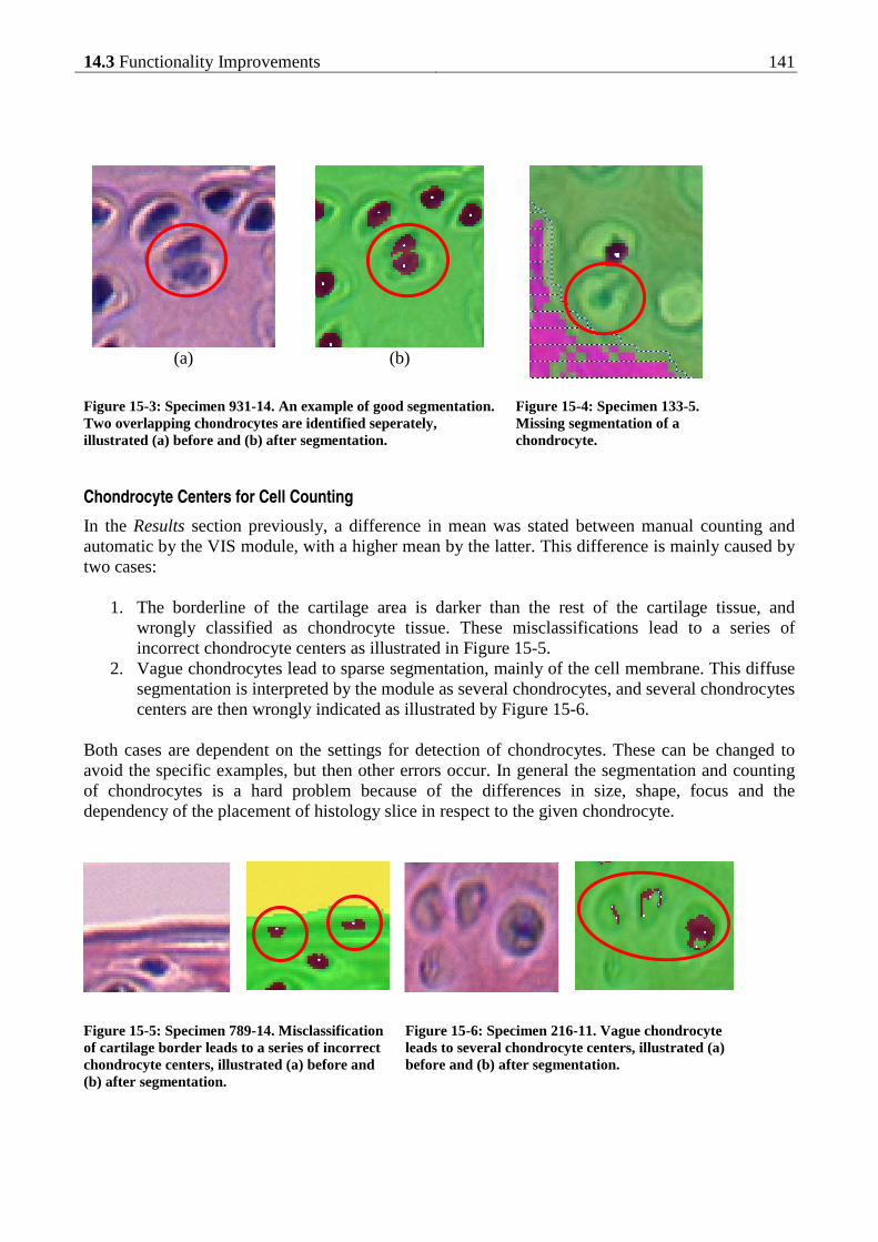
14.3 Functionality Improvements 141
(a)
(b)
Figure 15-3: Specimen 931-14. An example of good segmentation. Two overlapping chondrocytes are identified seperately, illustrated (a) before and (b) after segmentation.
Figure 15-4: Specimen 133-5. Missing segmentation of a chondrocyte.
Chondrocyte Centers for Cell Counting
In the Results section previously, a difference in mean was stated between manual counting and automatic by the VIS module, with a higher mean by the latter. This difference is mainly caused by two cases:
1. The borderline of the cartilage area is darker than the rest of the cartilage tissue, and wrongly classified as chondrocyte tissue. These misclassifications lead to a series of incorrect chondrocyte centers as illustrated in Figure 15-5.
2. Vague chondrocytes lead to sparse segmentation, mainly of the cell membrane. This diffuse segmentation is interpreted by the module as several chondrocytes, and several chondrocytes centers are then wrongly indicated as illustrated by Figure 15-6.
Both cases are dependent on the settings for detection of chondrocytes. These can be changed to avoid the specific examples, but then other errors occur. In general the segmentation and counting of chondrocytes is a hard problem because of the differences in size, shape, focus and the dependency of the placement of histology slice in respect to the given chondrocyte.
Figure 15-5: Specimen 789-14. Misclassification of cartilage border leads to a series of incorrect chondrocyte centers, illustrated (a) before and (b) after segmentation.
Figure 15-6: Specimen 216-11. Vague chondrocyte leads to several chondrocyte centers, illustrated (a) before and (b) after segmentation.

Evaluation of Segmentation
142
Bone Tissue
No cases of interest were observed in the evaluation of bone tissue segmentation.
Lacunae
Segmentation of the lacunae in the bone tissue is only at low priority, but misclassification can lead to wrong measures of tissue with higher priority. The misclassification concerns either the lacunae nucleus or the lacunae background. Cases of the first are illustrated and commented in Figure 15-7, whereas the latter is commented by Figure 15-8 and Figure 15-9.
(a)
(b)
(a)
(b)
Figure 15-8: Specimen 862-17. Lacunae incorrect segmented as cell tissue. Illustrated (a) before and (b) after segmentation.
Figure 15-9: Specimen 862-14. Lacunae incorrect segmented as cartilage tissue. Illustrated (a) before and (b) after segmentation.
Identification of the Tibia Cartilage Region
This part of the segmentation is the hardest and considered as the most important. Minor errors can easily be corrected by manual corrections though. Five cases are addressed of which the four first needs minor and the last needs major corrections:
1. Top of tibia cartilage is excluded from the marked region because of the assumption of an umbrella shape as described in Applied Methods. Illustrated in Figure 15-10a.
2. Part of the meniscus is close to the tibia cartilage, and is for this reason included by the mask. Illustrated in Figure 15-10b.
(a)
(b)
Figure 15-7: Lacunae nucleus tissue misclassified wrong in two cases: (a) Specimen 931-17, as cell tissue. (b) Specimen 985-11, as lacunae background.

14.3 Functionality Improvements 143
3. Steps in the post processing include area between the segmented cartilage region and the joint space, if assumed to be a part of the region. In some cases this is incorrect and results in a jagged region marking towards the joint-space. Illustrated in Figure 15-10c.
4. The defined region mask includes too much of the cartilage towards the right part of the image. Illustrated in Figure 15-10d.
5. Both femoral and tibia region are marked as only one region. This happens if the femoral and tibia regions are connected in most of the area. Illustrated in Figure 15-10e.
(a)
(b)
(c)
(d)
(e)
Figure 15-10: Examples of special cases of identification of the tibia cartilage region. Cropped images are taken from following specimens: (a) 133-11 (b) 216-8 (c) 137-20 (d) 213-2 (e) 174-20
Meniscus
Tibia Tibia
Tibia
Femur
Tibia
Tibia

Evaluation of Segmentation
144

Appendix F
Results – Cartilage Matrix Structure
This appendix contains the calculated results from the cartilage matrix structure measurements described in Chapter 7. Some of the methods are based upon thickness measurements of the cartilage matrix, which is defined as X in the following. The following methods have been applied and stated by results in this appendix:
• Fibrillation Index (FI) • Overall variance of X • Slope of X • Ln to the variance of the first numerical derivative of X (LTV).
The results are divided by following analysis parts:
• Correlation with pathology score o Normal distribution verification o Basic statistics o Box plot of distributions
• Treatment effect o Normal distribution verification o Basic statistics o Box plot of distributions
The plots are small because of limited space in the appendix. This makes the labels hard to see and they have been chosen to be removed. Instead examples of normal score plot and histogram are illustrated below. These can be used as guidelines when evaluating the plots.
0 50 100 150 2003
3.5
4
4.5
5
5.5
6
6.5
7
Sorted observation number
Fea
ture
val
ue
0 2 4 6 8 10
0
10
20
30
40
50
60
70
Bins of calculated feature
Fre
quen
cy

Results – Cartilage Matrix Structure
146
Correlation with Pathology Score
Normal Distribution Verification
Normal score plots and histograms for the measurements grouped by manually given cartilage matrix pathology score (see Appendix B). The scoring has been performed by Sanofi Aventis according to the modified Mankin grading system described in section 3.1.1. The specimens in the study set only represents score 0, 1, 3, 6 and 8.
Fibrillation Index
Score 0 Score 1 Score 3 Score 6 Score 8
Nor
mal
sco
re
0 5 10 150.75
0.8
0.85
0.9
0.95
0 20 40 600.7
0.75
0.8
0.85
0.9
0.95
0 20 40 60
0.7
0.8
0.9
1
0 20 40 60 800.2
0.4
0.6
0.8
1
0 10 20 30 400.2
0.4
0.6
0.8
1
His
togr
am
0.75 0.8 0.85 0.9 0.950
1
2
3
4
5
0.7 0.8 0.9 10
5
10
15
0.7 0.8 0.9 10
2
4
6
8
0.2 0.4 0.6 0.8 10
5
10
15
0.2 0.4 0.6 0.8 10
2
4
6
8
Overall Variance
Score 0 Score 1 Score 3 Score 6 Score 8
Nor
mal
sco
re
0 5 10 153
4
5
6
7
0 20 40 600
2
4
6
8
10
0 20 40 602
4
6
8
10
0 20 40 60 804
5
6
7
8
9
0 10 20 30 405
6
7
8
9
10
His
togr
am
3 4 5 6 70
1
2
3
0 5 100
2
4
6
8
10
2 4 6 8 100
2
4
6
8
10
4 6 8 100
2
4
6
8
10
4 6 8 100
2
4
6
8
10

14.3 Functionality Improvements 147
Slope of Thickness Measurement
Score 0 Score 1 Score 3 Score 6 Score 8
Nor
mal
sco
re
0 5 10 15-0.1
-0.05
0
0.05
0.1
0.15
0 20 40 60-0.2
-0.1
0
0.1
0.2
0 20 40 60-0.3
-0.2
-0.1
0
0.1
0.2
0 20 40 60 80-0.3
-0.2
-0.1
0
0.1
0 10 20 30 40-0.6
-0.4
-0.2
0
0.2
His
togr
am
-0.1 0 0.1 0.2 0.30
2
4
6
8
-0.2 -0.1 0 0.1 0.20
5
10
15
-0.4 -0.2 0 0.2 0.40
2
4
6
8
10
-0.3 -0.2 -0.1 0 0.10
5
10
15
20
-0.6 -0.4 -0.2 0 0.20
5
10
15
ln to the Trend Variance
Score 0 Score 1 Score 3 Score 6 Score 8
Nor
mal
sco
re
0 5 10 15-3
-2.5
-2
-1.5
-1
-0.5
0 20 40 60-3
-2
-1
0
0 20 40 60-3
-2
-1
0
1
2
0 20 40 60 80-2
-1
0
1
2
3
0 10 20 30 400
1
2
3
His
togr
am
-3 -2 -1 00
1
2
3
-3 -2 -1 00
2
4
6
8
10
-4 -2 0 20
2
4
6
8
10
-2 0 2 40
5
10
15
0 1 2 30
2
4
6
8
Basic statistics and box plot
Fibrillation Index
Manually given pathology score
0 1 3 6 8
N 11 48 43 62 37
Min 0.78 0.72 0.62 0.35 0.29
Max 0.93 0.93 0.94 0.91 0.80
Mean 0.89 0.85 0.80 0.61 0.51
SD 0.042 0.056 0.082 0.128 0.118
Score 0 Score 1 Score 3 Score 6 Score 8
0.3
0.4
0.5
0.6
0.7
0.8
0.9
Fib
rilla
tion
Inde
x (F
I)

Results – Cartilage Matrix Structure
148
Overall Variance
Manually given pathology score
0 1 3 6 8
N 11 48 43 62 37
Min 3.43 1.24 3.44 4.35 5.87
Max 6.58 8.08 8.18 8.55 9.21
Mean 5.00 4.99 5.95 6.62 7.84
SD 0.95 1.50 0.95 0.96 0.75
Score 0 Score 1 Score 3 Score 6 Score 81
2
3
4
5
6
7
8
9
Var
ianc
e of
thi
ckne
ss
Slope of Thickness Measurement
Manually given pathology score
0 1 3 6 8
N 11 48 43 62 37
Min -0.06 -0.16 -0.22 -0.29 -0.43
Max 0.11 0.17 0.12 0.06 0.03
Mean 0.010 -0.015 -0.042 -0.079 -0.169
SD 0.044 0.066 0.076 0.074 0.090
Score 0 Score 1 Score 3 Score 6 Score 8
-0.4
-0.3
-0.2
-0.1
0
0.1
Slo
pe o
f th
ickn
ess
ln to the Trend Variance
Manually given pathology score
0 1 3 6 8
N 11 48 43 62 37
Min -2.68 -2.64 -2.04 -1.53 0.34
Max -0.77 -0.09 1.24 2.73 2.92
Mean -1.78 -1.43 -0.54 0.88 1.82
SD 0.47 0.60 0.88 0.87 0.66
Score 0 Score 1 Score 3 Score 6 Score 8
-2
-1
0
1
2
3
ln t
o tr
end
varia
nce
of t
hick
ness
(LT
V)

14.3 Functionality Improvements 149
Trend Statistic Tests
In the following two remarks are used: *These f-tests rejected the null-hypothesis on a 95% level of significance i.e. corresponding t-test is performed for unequal distribution.
**Notice that the tested means are opposite of the assumption in the thesis. In these cases the thesis is rejected and the results of the t-test are useless.
Fibrillation Index
F-test T-test Manually given pathology score
1 3 6 8
0 0.32 0.027* 0.0006* 0.0013*
1 - 0.013* <0.0001* <0.0001*
3 - - 0.0025* 0.021*
6 - - - 0.62
Manually given pathology score
1 3 6 8
1 0.11 <0.0001 <0.0001 <0.0001
3 - 0.0013 <0.0001 <0.0001
6 - - <0.0001 <0.0001
8 - - - <0.0001
Mann-Whitney Test
Manually given pathology score
1 3 6 8
0 0.0093 0.0004 <0.0001 <0.0001
1 - 0.0030 <0.0001 <0.0001
3 - - <0.0001 <0.0001
6 - - - 0.0002
Overall Variance
F-test T-test Manually given pathology score
1 3 6 8
0 0.12 0.91 0.94 0.30
1 - 0.003* 0.001* <0.0001*
3 - - 0.95 0.16
6 - - - 0.12
Manually given pathology score
1 3 6 8
1 0.49 0.0023 <0.0001 <0.0001
3 - 0.0002 <0.0001 <0.0001
6 - - 0.0003 <0.0001
8 - - - <0.0001
Mann-Whitney Test
Manually given pathology score
1 3 6 8
0 0.49 0.0047 <0.0001 <0.0001
1 - 0.0003 <0.0001 <0.0001
3 - - 0.0003 <0.0001
6 - - - <0.0001

Results – Cartilage Matrix Structure
150
Slope of Thickness Measurement
F-test T-test Manually given pathology score
1 3 6 8
0 0.18 0.071 0.078 0.021*
1 - 0.33 0.37 0.039*
3 - - 0.87 0.27
6 - - - 0.18
Manually given pathology score
1 3 6 8
1 0.12 0.018 0.0001 <0.0001
3 0.034 <0.0001 <0.0001
6 0.0077 <0.0001
8 <0.0001
Mann-Whitney Test Manually given pathology score
1 3 6 8
0 0.14 0.0072 <0.0001 <0.0001
1 - 0.027 <0.0001 <0.0001
3 - - 0.010 <0.0001
6 - - - <0.0001
ln to the Trend Variance
F-test T-test Manually given pathology score
1 3 6 8
0 0.44 0.042* 0.034* 0.26
1 0.011* 0.0074* 0.50
3 0.97 0.089
6 0.075
Manually given pathology score
1 3 6 8
1 0.037 <0.0001 <0.0001 <0.0001
3 <0.0001 <0.0001 <0.0001
6 <0.0001 <0.0001
8 <0.0001
Mann-Whitney Test Manually given pathology score
1 3 6 8
0 0.028 <0.0001 <0.0001 <0.0001
1 - <0.0001 <0.0001 <0.0001
3 - - <0.0001 <0.0001
6 - - - <0.0001

14.3 Functionality Improvements 151
Treatment Effect
Normal Distribution Verification
Fibrillation Index
Control Treated
Nor
mal
sco
re
0 50 1000.2
0.4
0.6
0.8
1
0 50 100 1500.2
0.4
0.6
0.8
1
His
togr
am
0.2 0.4 0.6 0.8 10
5
10
15
0.2 0.4 0.6 0.8 10
10
20
30
Overall Variance
Control Treated
Nor
mal
sco
re
0 50 1000
2
4
6
8
10
0 50 100 1502
4
6
8
10
His
togr
am
0 5 100
5
10
15
20
25
2 4 6 8 100
5
10
15
20
Slope of Thickness Measurement
Control Treated
Nor
mal
sco
re
0 50 100-0.6
-0.4
-0.2
0
0.2
0 50 100 150-0.4
-0.2
0
0.2
0.4
His
togr
am
-0.6 -0.4 -0.2 0 0.20
10
20
30
40
-0.4 -0.2 0 0.2 0.40
10
20
30
40

Results – Cartilage Matrix Structure
152
Ln to the Trend Variance
Control Treated
Nor
mal
sco
re
0 50 100-4
-2
0
2
4
0 50 100 150-4
-2
0
2
4
His
togr
am
-4 -2 0 2 40
5
10
15
20
-4 -2 0 2 40
5
10
15
20
Basic statistics and box plot
Fibrillation Index
Control Treated
n 100 101
Min 0.31 0.29
Max 0.93 0.94
Mean 0.67 0.74
SD 0.17 0.17
Control Treated
0.3
0.4
0.5
0.6
0.7
0.8
0.9
Fib
rilla
tion
Inde
x (F
I)
Overall Variance
Control Treated
n 100 101
Min 1.24 2.93
Max 8.58 9.21
Mean 6.32 6.13
SD 1.49 1.44
Control Treated1
2
3
4
5
6
7
8
9
Var
ianc
e of
thi
ckne
ss

14.3 Functionality Improvements 153
Slope of Thickness Measurement
Control Treated
n 100 101
Min -0.43 -0.33
Max 0.11 0.17
Mean -0.082 -0.053
SD 0.084 0.098
Control Treated
-0.4
-0.3
-0.2
-0.1
0
0.1
Slo
pe o
f th
ickn
ess
Ln to the Trend Variance
Control Treated
n 100 101
Min -2.68 -2.64
Max 2.92 2.53
Mean 0.39 -0.29
SD 1.40 1.46
Control Treated
-2
-1
0
1
2
3ln
to
tren
d va
rianc
e of
thi
ckne
ss (
LTV
)

Results – Cartilage Matrix Structure
154

Appendix G
Results – Cellularity of Chondrocytes
This appendix contains the calculated results from the measurements of the cellularity of chondrocytes described in Chapter 1. The performed measurement is an area fraction of the chondrocyte area divided by the cartilage area and is defined as Y in the following. The following methods have been applied and stated by results in this appendix:
• Overall average of Y • Normalized slope of Y • Threshold of Y
The results are divided by following analysis parts:
• Correlation with pathology score o Normal distribution verification o Basic statistics o Box plot of distributions
• Treatment effect o Normal distribution verification o Basic statistics o Box plot of distributions
The plots are small because of limited space in the appendix. This makes the labels hard to see and they have been chosen to be removed. Instead examples of normal score plot and histogram are illustrated below. These can be used as guidelines when evaluating the plots.
0 50 100 150 2003
3.5
4
4.5
5
5.5
6
6.5
7
Sorted observation number
Fea
ture
val
ue
0 2 4 6 8 10
0
10
20
30
40
50
60
70
Bins of calculated feature
Fre
quen
cy

Results – Cellularity of Chondrocytes
156
Correlation with Pathology Score
Normal Distribution Verification
Normal score plots and histograms for the measurements grouped by manually given cellularity pathology score (see Appendix B). The scoring has been performed by Sanofi Aventis according to the modified Mankin grading system described in section 3.1.1. The specimens in the study set only represents score 0, 2 and 5.
Overall Average
Score 0 Score 3 Score 8
Nor
mal
sco
re
0 5 100.03
0.035
0.04
0.045
0.05
0.055
0 50 100 150 2000.01
0.02
0.03
0.04
0.05
0.06
0 10 20 30 400.01
0.02
0.03
0.04
His
togr
am
0.03 0.04 0.05 0.060
0.5
1
1.5
2
0 0.02 0.04 0.060
10
20
30
40
0.01 0.02 0.03 0.040
2
4
6
8
10
Normalized Slope
Score 0 Score 3 Score 8
Nor
mal
sco
re
0 5 10-4
-2
0
2
4
6 x 10⁻⁴
0 50 100 150 200-4
-2
0
2
4x 10⁻³
0 10 20 30 40-4
-3
-2
-1
0
1x 10⁻³
His
togr
am
-5 0 5 10
x 10-4
0
0.5
1
1.5
2
-4 -2 0 2 4
x 10-3
0
10
20
30
40
-4 -2 0 2
x 10-3
0
2
4
6
8
10

14.3 Functionality Improvements 157
By Threshold
Score 0 Score 3 Score 8
Nor
mal
sco
re
0 5 10
0.65
0.7
0.75
0.8
0 50 100 150 200
0
0.2
0.4
0.6
0.8
0 10 20 30 400
0.2
0.4
0.6
0.8
His
togr
am
0.65 0.7 0.75 0.80
0.5
1
1.5
2
0 0.2 0.4 0.6 0.80
10
20
30
40
0 0.2 0.4 0.6 0.80
2
4
6
8

Results – Cellularity of Chondrocytes
158
Basic statistics and box plot
Overall Average
Manually given pathology score 0 2 5
N 9 152 40
Min 0.032 0.012 0.012
Max 0.051 0.053 0.036
Mean 0.043 0.032 0.024
SD 0.0055 0.0083 0.0050
Score 0 Score 2 Score 50.01
0.02
0.03
0.04
0.05
Ave
rage
cel
lula
rity
Normalized Slope
Manually given pathology score 0 2 5
N 9 152 40
Min -0.0003 -0.0033 -0.0032
Max 0.0005 0.0021 0.0008
Mean 0.00009 -0.00077 -0.00145
SD 2.3·10-4 8.9·10-4 8.5·10-4
Score 0 Score 2 Score 5
-3
-2
-1
0
1
2
x 10-3
Slo
pe o
f ce
llula
rity
By threshold
Manually given pathology score 0 2 5
N 9 152 40
Min 0.66 0.17 0.20
Max 0.80 0.78 0.62
Mean 0.73 0.57 0.44
SD 0.05 0.13 0.10
Score 0 Score 2 Score 5
0.2
0.3
0.4
0.5
0.6
0.7
0.8
Cel
lula
rity
by t
hres
hold

14.3 Functionality Improvements 159
Treatment Effect
Normal Distribution Verification
Overall Average
Control Treated
Nor
mal
sco
re
0 50 1000.01
0.02
0.03
0.04
0.05
0.06
0 50 100 1500.01
0.02
0.03
0.04
0.05
0.06
His
togr
am
0 0.02 0.04 0.060
5
10
15
20
25
0 0.02 0.04 0.060
5
10
15
20
25
Normalized Slope
Control Treated
Nor
mal
sco
re
0 50 100-4
-3
-2
-1
0
1x 10⁻³
0 50 100 150-4
-2
0
2
4x 10⁻³
His
togr
am
-4 -2 0 2
x 10-3
0
5
10
15
20
-4 -2 0 2 4
x 10-3
0
5
10
15
20
25
By Threshold
Control Treated
Nor
mal
sco
re
0 50 1000.2
0.4
0.6
0.8
1
0 50 100 1500
0.2
0.4
0.6
0.8
His
togr
am
0.2 0.4 0.6 0.8 10
5
10
15
20
0 0.2 0.4 0.6 0.80
5
10
15
20
25

Results – Cellularity of Chondrocytes
160
Basic statistics and box plot
Overall Average
Control Treated
n 100 101
Min 0.015 0.012
Max 0.053 0.051
Mean 0.030 0.032
SD 0.0081 0.0091
Control Treated0.01
0.02
0.03
0.04
0.05
Ave
rage
cel
lula
rity
Normalized Slope
Control Treated
n 100 101
Min -3.3·10-3 -3.1·10-3
Max 9.6·10-4 2.1·10-3
Mean -1.1·10-3 -6.4·10-4
SD 9.0·10-4 8.9·10-4
Control Treated
-3
-2
-1
0
1
2
x 10-3
Slo
pe o
f ce
llula
rity
By Threshold
Control Treated
n 100 101
Min 0.238 0.172
Max 0.799 0.772
Mean 0.548 0.563
SD 0.120 0.148
Control Treated
0.2
0.3
0.4
0.5
0.6
0.7
0.8
Cel
lula
rity
by t
hres
hold

Appendix H
Results – Subchondral Bone Structure
This appendix contains the calculated results from the analysis of the subchondral bone density described in Chapter 9. The result of the subchondral bone measurement is defined as Z in the following. The following methods have been applied and stated by results in this appendix:
• Overall average of Z • Slope of Z
The results are divided by following analysis parts:
• Correlation with pathology score o Normal distribution verification o Basic statistics o Box plot of distributions
• Treatment effect o Normal distribution verification o Basic statistics o Box plot of distributions
The plots are small because of limited space in the appendix. This makes the labels hard to see and they have been chosen to be removed. Instead examples of normal score plot and histogram are illustrated below. These can be used as guidelines when evaluating the plots.
0 50 100 150 2003
3.5
4
4.5
5
5.5
6
6.5
7
Sorted observation number
Fea
ture
val
ue
0 2 4 6 8 10
0
10
20
30
40
50
60
70
Bins of calculated feature
Fre
quen
cy

Results – Subchondral Bone Structure
162
Correlation with Pathology Score
Normal Distribution Verification
Normal score plots and histograms for the measurements grouped by manually given bone pathology score (see Appendix B). The scoring has been performed by Sanofi Aventis according to the modified Mankin grading system described in section 3.1.1. The specimens in the study set only represents score 0, 2 and 5.
Overall Average
Score 0 Score 3 Score 8
Nor
mal
sco
re
1 2 3 40.4
0.45
0.5
0.55
0.6
0 50 1000.4
0.5
0.6
0.7
0.8
0.9
0 50 100 1500.5
0.6
0.7
0.8
0.9
1
His
togr
am
0.4 0.45 0.5 0.55 0.60
0.5
1
1.5
2
0.4 0.6 0.8 10
5
10
15
20
0.4 0.6 0.8 10
10
20
30
Slope
Score 0 Score 3 Score 8
Nor
mal
sco
re
1 2 3 4-1
-0.5
0
0.5
1x 10⁻⁴
0 50 100-1
-0.5
0
0.5
1
1.5x 10⁻³
0 50 100 150-1
-0.5
0
0.5
1
1.5 x 10⁻³
His
togr
am
-1 -0.5 0 0.5 1
x 10-4
0
0.5
1
1.5
2
-1 0 1 2
x 10-3
0
5
10
15
20
25
-1 0 1 2
x 10-3
0
10
20
30
40

14.3 Functionality Improvements 163
Basic statistics and box plot
Overall Average
Manually given pathology score 0 3 8
N 4 92 105
Min 0.43 0.40 0.54
Max 0.52 0.90 0.99
Mean 0.48 0.67 0.83
SD 0.05 0.11 0.08
Score 0 Score 3 Score 8
0.4
0.5
0.6
0.7
0.8
0.9
1
Ave
rage
bon
e de
nsity
Slope
Manually given pathology score 0 3 8
N 4 92 105
Min -7.63·10-5 -6.52·10-4 -8.52·10-4
Max 6.22·10-5 1.18·10-3 1.45·10-3
Mean 1.02·10-5 2.78·10-4 3.74·10-4
SD 6.2·10-5 3.72·10-4 2.90·10-4
Score 0 Score 3 Score 8
-5
0
5
10
15x 10
-4
Slo
pe o
f bo
ne d
ensi
ty
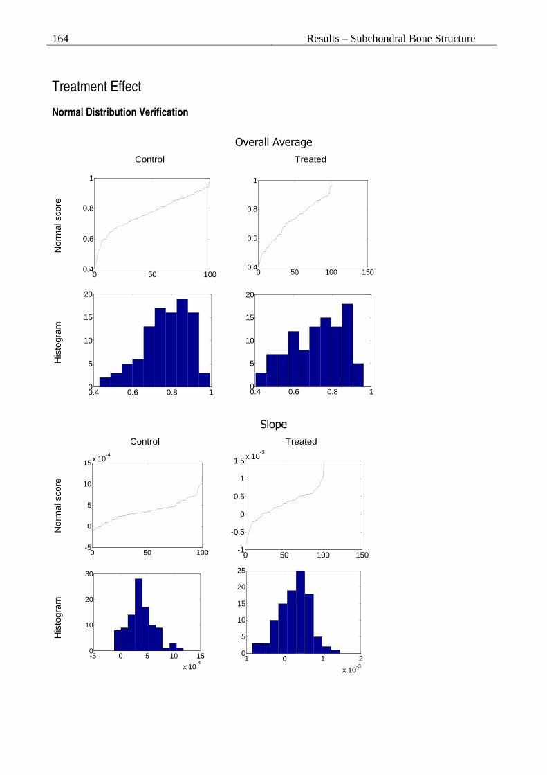
Results – Subchondral Bone Structure
164
Treatment Effect
Normal Distribution Verification
Overall Average
Control Treated
Nor
mal
sco
re
0 50 1000.4
0.6
0.8
1
0 50 100 150
0.4
0.6
0.8
1
His
togr
am
0.4 0.6 0.8 10
5
10
15
20
0.4 0.6 0.8 10
5
10
15
20
Slope
Control Treated
Nor
mal
sco
re
0 50 100-5
0
5
10
15x 10-4
0 50 100 150-1
-0.5
0
0.5
1
1.5x 10⁻³
His
togr
am
-5 0 5 10 15
x 10-4
0
10
20
30
-1 0 1 2
x 10-3
0
5
10
15
20
25

14.3 Functionality Improvements 165
Basic statistics and box plot
Overall Average
Control Treated
n 100 101
Min 0.43 0.40
Max 0.99 0.96
Mean 0.77 0.72
SD 0.12 0.14
Control Treated
0.4
0.5
0.6
0.7
0.8
0.9
1
Ave
rage
bon
e de
nsity
Slope of Bone Density
Control Treated
n 100 101
Min -1,2·10-4 -8,5·10-4
Max 1,2·10-3 1,5·10-3
Mean 3,8·10-4 2,7·10-4
SD 2,5·10-4 3,9·10-4
Control Treated
-5
0
5
10
15x 10
-4
Slo
pe o
f bo
ne d
ensi
ty

Results – Subchondral Bone Structure
166

Appendix I
CD-ROM Contents
A CD-ROM is included in the print for the examination evaluation by my supervisor, sensor and additionally for Visiopharm. The CD-ROM contains the following grouped by folders:
Images Example images of the specimens that has been used as data in the thesis. Images from three mice are included:
• 103 – Medium OA affected • 174 – Mild OA affected • 196 – Severe OA affected
Module This includes all the source code of the OA Quantifier module, and a Microsoft Visual Studio 2003 project that includes the source code files.
Poster The poster and abstract submitted for the OARSI 11th World Congress on Osteoarthritis, 2006, in Prague. The poster is in three formats of same version: .ppt, .pdf, and .png. The abstract is in plain text (ASCII).
Report The final report of the thesis is included in two formats: .doc and .pdf.
Study data Data for the applied study set:
• STR1N-25-2005-score1.xls - A scoring list of the specimens, for all three parameters of joint degradation (cartilage matrix, cellularity and subchondral bone).
• STR-1N-25-2005-Decode.xls – Decode list for groups of control and treated.
• tibia_new_score.xls – Revised scoring list (cartilage matrix and cellularity scores only).

CD-ROM Contents
168
Visiopharm Includes information materials and poster used in the work of this thesis from the Visiopharm site: www.visiopharm.dk. The following files are included:
• AutomatedHistomorphometry.pdf • posteroarsi-2003-bone.pdf • posteroarsi-2003-cartilage.pdf • posteroarsi-2004-histo.pdf • vis_web.pdf

Appendix J
Poster for OARSI conference in Prague, 2006
A draft poster was prepared in the beginning of July 2006 for the OARSI 11th World Congress on Osteoarthritis, 2006, in Prague, with detailed information of the applied and proposed quantitative histomorphometric measurements and end points. The poster is seen on the following page. An abstract was submitted in the end of July 2006 describing the contents of the poster. The abstract is similar to the abstract in this thesis and is not included in the report.

Poster for OARSI conference in Prague,
170