Embed Size (px)
Citation preview

HAL Id: hal-00963542https://hal.archives-ouvertes.fr/hal-00963542
Submitted on 3 Jun 2014
HAL is a multi-disciplinary open accessarchive for the deposit and dissemination of sci-entific research documents, whether they are pub-lished or not. The documents may come fromteaching and research institutions in France orabroad, or from public or private research centers.
L’archive ouverte pluridisciplinaire HAL, estdestinée au dépôt et à la diffusion de documentsscientifiques de niveau recherche, publiés ou non,émanant des établissements d’enseignement et derecherche français ou étrangers, des laboratoirespublics ou privés.
Automated Estimation of Collagen Fibre Dispersion inthe Dermis and its Contribution to the Anisotropic
Behaviour of SkinAisling Ni’ Annaidh, Karine Bruyere, Michel Destrade, Michael D. Gilchrist,
Corrado Maurini, Mélanie Ottenio, Giuseppe Saccomandi
To cite this version:Aisling Ni’ Annaidh, Karine Bruyere, Michel Destrade, Michael D. Gilchrist, Corrado Maurini, etal.. Automated Estimation of Collagen Fibre Dispersion in the Dermis and its Contribution to theAnisotropic Behaviour of Skin. Annals of Biomedical Engineering, Springer Verlag, 2012, 40 (8), pp.1666-1678. �10.1007/s10439-012-0542-3�. �hal-00963542�
Automated Estimation of Collagen Fibre Dispersion
in the Dermis and its Contribution to the Anisotropic
Behaviour of Skin
Aisling Nı Annaidh 1,2,3, Karine Bruyere4, Michel Destrade5,1, Michael D.
Gilchrist1, Corrado Maurini2,3, Melanie Ottenio4, and Giuseppe Saccomandi7
1School of Mechanical & Materials Engineering, University College Dublin,
Belfield, Dublin 4, Ireland
2UPMC, Univ Paris 6, UMR 7190, Institut Jean Le Rond d’Alembert, Boıte
courrier 161-2, 4 Place Jussieu, F-75005, Paris France
3CNRS, UMR 7190, Institut Jean Le Rond d’Alembert, Boıte courrier 161-2,
4 Place Jussieu, F-75005, Paris France
4Universite de Lyon, F-69622, Lyon, France, Ifsttar, LBMC, UMR T9406,
F-69675, Bron, Universite Lyon 1, Villeurbanne
5School of Mathematics, Statistics and Applied Mathematics, National
University of Ireland Galway, Galway, Ireland
6School of Human Kinetics, University of Ottawa, Ontario K1N 6N5, Canada
7Dipartimento di Ingegneria Industriale, Universita degli Studi di Perugia,
06125 Perugia, Italy
1

Abstract
Collagen fibres play an important role in the mechanical behaviour of many soft tis-
sues. Modelling of such tissues now often incorporates a collagen fibre distribution. How-
ever, the availability of accurate structural data has so far lagged behind the progress
of anisotropic constitutive modelling. Here, an automated process is developed to iden-
tify the orientation of collagen fibres using inexpensive and relatively simple techniques.
The method uses established histological techniques and an algorithm implemented in the
MATLAB image processing toolbox. It takes an average of 15 seconds to evaluate one
image, compared to several hours if assessed visually. The technique was applied to his-
tological sections of human skin with different Langer line orientations and a definite cor-
relation between the orientation of Langer lines and the preferred orientation of collagen
fibres in the dermis (P<0.001, R2= 0.95) was observed. The structural parameters of the
Gasser-Ogden-Holzapfel (GOH) model were all successfully evaluated. The mean disper-
sion factor for the dermis was κ = 0.1404 ± 0.0028. The constitutive parameters µ , k1 and
k2 were evaluated through physically-based, least squares curve-fitting of experimental test
data. The values found for µ , k1 and k2 were 0.2014 MPa, 243.6 and 0.1327, respectively.
Finally, the above model was implemented in ABAQUS/ Standard and a finite element
(FE) computation was performed of uniaxial extension tests on human skin. It is expected
that the results of this study will assist those wishing to model skin, and that the algorithm
described will be of benefit to those who wish to evaluate the collagen dispersion of other
soft tissues.
Keywords: Fibre Orientation, Anisotropic, Skin, Collagen Fibres
2

1 Introduction
Collagen fibres govern many of the mechanical properties of soft tissues, in particular their
anisotropic behaviour. Due to the complex nature of fibre arrangements, such tissues are often
represented as either isotropic or transversely isotropic [6, 2, 3]. The availability of quantitative
structural data on the orientation and concentration of collagen fibres is crucial in order to
describe the behaviour of these soft tissues accurately.
A number of studies have used statistical distributions to describe the fibre arrangement in
soft tissues. Lanir [19] was the first to attempt to account for fibre dispersion. Lanir’s method
expresses the mechanical response in terms of angular integrals. This technique accounts for
the contribution of infinitesimal fractions of collagen fibres in a particular orientation. This ap-
proach leads to accurate results but it is not a practical option for efficient numerical implemen-
tation [4]. The second approach uses generalised structure tensors (GST), which are assumed
to represent the three-dimensional distribution of the fibres. The strain energy function is then
calculated by using the average stretch rather than by using a stretch for each individual fibre.
GST is a simpler method than Lanir’s, and is easily implemented in FE algorithms [10].
In this paper we implement the GST method proposed by Gasser et al [10], described in
detail in Section 2.3. In that model, structural parameters such as the fibre dispersion parameter
and mean orientation of fibres are required. In order to quantify the orientations of collagen fi-
bres in the human dermis an automated process is developed for detecting collagen orientations
in histology slides.
Histology is the microscopic study of cells and tissue. It is an important diagnostic tool in
medicine which is utilised here for the purpose of analysing collagen orientation. Traditionally,
histology slides are examined by expert observers who assess individual slides visually. This
method is both time consuming and subjective. An automated process would enable large vol-
umes of images to be analysed quickly and improve the objectivity of the task. Much research
has been conducted recently on imaging techniques of biological soft tissue for the extraction
of structural data; however these techniques require either expensive equipment or manual post
processing [8, 28, 29, 30]. There has been little research to date carried out on the automated
analysis of histology slides. Four notable exceptions are the work of Van Zuijlen et al [27],
3
Noorlander et al [22], Elbischger et al [5] and Jor et al [17].
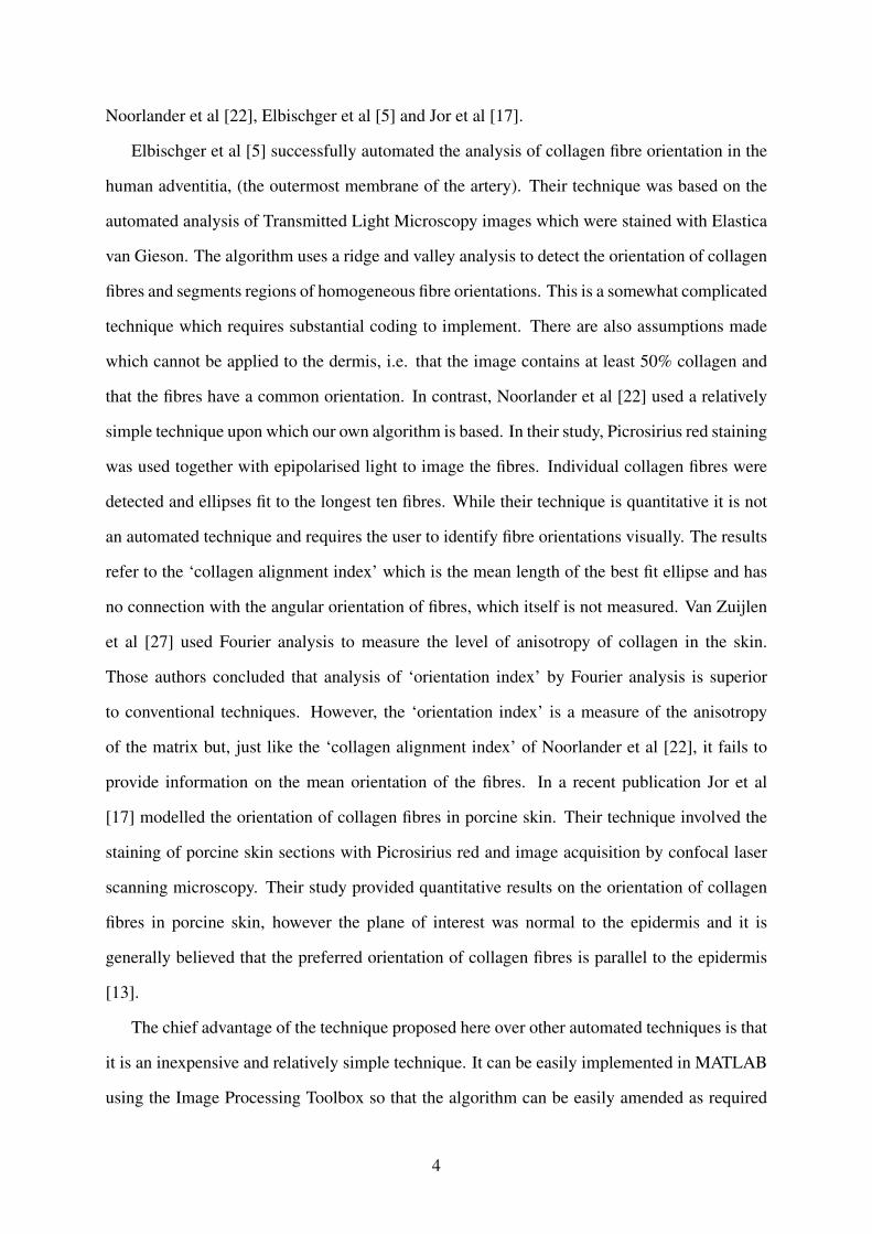
Elbischger et al [5] successfully automated the analysis of collagen fibre orientation in the
human adventitia, (the outermost membrane of the artery). Their technique was based on the
automated analysis of Transmitted Light Microscopy images which were stained with Elastica
van Gieson. The algorithm uses a ridge and valley analysis to detect the orientation of collagen
fibres and segments regions of homogeneous fibre orientations. This is a somewhat complicated
technique which requires substantial coding to implement. There are also assumptions made
which cannot be applied to the dermis, i.e. that the image contains at least 50% collagen and
that the fibres have a common orientation. In contrast, Noorlander et al [22] used a relatively
simple technique upon which our own algorithm is based. In their study, Picrosirius red staining
was used together with epipolarised light to image the fibres. Individual collagen fibres were
detected and ellipses fit to the longest ten fibres. While their technique is quantitative it is not
an automated technique and requires the user to identify fibre orientations visually. The results
refer to the ‘collagen alignment index’ which is the mean length of the best fit ellipse and has
no connection with the angular orientation of fibres, which itself is not measured. Van Zuijlen
et al [27] used Fourier analysis to measure the level of anisotropy of collagen in the skin.
Those authors concluded that analysis of ‘orientation index’ by Fourier analysis is superior
to conventional techniques. However, the ‘orientation index’ is a measure of the anisotropy
of the matrix but, just like the ‘collagen alignment index’ of Noorlander et al [22], it fails to
provide information on the mean orientation of the fibres. In a recent publication Jor et al
[17] modelled the orientation of collagen fibres in porcine skin. Their technique involved the
staining of porcine skin sections with Picrosirius red and image acquisition by confocal laser
scanning microscopy. Their study provided quantitative results on the orientation of collagen
fibres in porcine skin, however the plane of interest was normal to the epidermis and it is
generally believed that the preferred orientation of collagen fibres is parallel to the epidermis
[13].
The chief advantage of the technique proposed here over other automated techniques is that
it is an inexpensive and relatively simple technique. It can be easily implemented in MATLAB
using the Image Processing Toolbox so that the algorithm can be easily amended as required
4

for the user’s specific application. It is a fully automated process (aside from the image ac-
quisition phase) and is capable of analysing a greater number of images, and faster, than a
manual analysis. It also eliminates the subjectivity which is present using traditional meth-
ods. The technique provides quantitative data on both the collagen orientation and the level of
anisotropy in the dermis, but it could be easily amended to identify any tissues/objects within
other soft tissues.
Due to the anisotropic properties of collagen based soft tissues [21], modelling now often
incorporates a collagen fibre distribution. The accuracy of these structural models rely heavily
on knowledge of collagen fibre orientations. While this data has recently been published for
porcine skin by Jor et al [17], to the best of the authors’ knowledge, quantitative data on the
orientation of collagen fibres in the human dermis has not been previously published. With the
quantitative data obtained here, structural parameters such as γ and κ from the Gasser-Ogden-
Holzapfel model [10] can be evaluated independently. This structural data, coupled with the
mechanical testing of the same skin samples [21] provides us with sufficient data to model
human skin using the GOH model.
2 Materials & Methods
2.1 Tensile tests and histology
In vitro tensile tests of human skin were performed using a Universal Tensile Test machine at
a strain rate of 0.012s−1. The tensile load was measured with a 1kN piezoelectric load cell and
the strain was measured via a displacement actuator. Skin biopsies were excised adjacent to the
tensile test samples and stained with Van Gieson to dye collagen fibres pink/red. Further details
of the tensile test experimental procedure and histology protocol are outlined in Nı Annaidh
et al [21].
2.2 Automated detection of fibre orientations
Images were taken of slides parallel to the epidermis (see Section 2.4) using an Aperop ScanScope
XT scanner and ScanScope software. This slide scanner has the ability to scan up to 120 slides
5

automatically. The images to be analysed were selected from the reticular layer of the der-
mis which forms the main structural body of the skin. The optical magnification used was 5x,
which is quite low; however, this was the optimal magnification to obtain a large enough field
of view to be representative while also maintaining enough detail to recognise the boundaries
of fibre bundles. Multiple images were taken of each sample in order to capture the entire area.
The field of view for each image taken at this magnification was 2.24 mm2. The orientation of
collagen fibres were then calculated in a fully-automated customised MATLAB routine using
the Image Processing Toolbox. The algorithm is described below and is illustrated in Fig. 1.
• A global threshold level was computed using the graythresh function. This function
chooses a global image threshold using Otsu’s method which aims to minimise the intr-
aclass variance of black and white pixels [24]. This automatically distinguishes collagen
fibres from other areas which are not of interest in the analysis, such as cells or histo-
logical ground substance. The image was then binarised based on this threshold level
producing an image containing black pixels for collagen and white pixels for all other
areas;
• Morphological operations were performed on the binary image using the bwmorph func-
tion. An erosion step was performed to detach cross-linking fibres from each other. This
step removed pixels from the boundaries using a structural element of size 3 pixels x
3 pixels. One iteration only of this step was performed which was the optimal number
of iterations to detach cross-linking fibres while also leaving smaller fibres intact. The
second morphological operation was performed using the imfill function. This function
fills in the ‘holes’ within the binary image, where a hole is defined as a set of isolated
pixels which cannot be reached by filling in the background pixels from the edge. This
step resulted in a ‘cleaner’ image to analyse.
• Individual fibre bundles are identified using bwlabel. This function identifies connected
components (8-connected) in a 2D binary image and labels each component individually.
It uses the general procedure outlined by Haralick and Shapiro [12];
• The regionprops function outputs a set of properties for each labelled component. The
6

function also fits an ellipse to each component by matching the second order moments of
that component to an equivalent ellipse following the procedure by Haralick and Shapiro
[12];
• Only ellipses which were elongated and of a certain area were selected 1;
• The orientation of the major axis of each ellipse was calculated and taken as the ap-
proximate orientation of each component. The advantage of fitting an ellipse about each
component is that the orientation is measured in a systematic and repeatable manner
which can account for the non-uniformities of the shape of each component;
• The orientations of each component was then plotted on a histogram (see Fig. 2). Two
distinct peaks were evident from this figure. It is assumed that these two peaks corre-
spond to the preferred orientation of two crossing families of fibres as shown in Fig. 3. A
von Mises probability density function was fit to the data and the mean orientation and
dispersion factor were calculated as described in Section 2.4.
Validation
As explained by Van Zuijlen et al [27], there are difficulties involved with validating automated
techniques because the true result of each histology slide is unknown. For the validation of their
algorithm, computer generated images representing collagen fibres with known orientations
were used. However, in order to create an accurate computer generated image, a model which
represents the structure of the collagen matrix is required, but no such model exists [5]. To
validate our technique, a selection of slides in the plane perpendicular to the epidermis (see
Fig. 4) were manually segmented and their mean orientation compared to those calculated
through the automated process. Although it is the plane parallel to the epidermis that is used
for the collection of structural data, the perpendicular plane was chosen for validation purposes
because in general it displays a more orientated pattern and is easier to segment manually.
1Out-of-plane fibres manifest themselves as circular areas. This condition was introduced to exclude out-of-plane fibres from the analysis. A sensitivity analysis was carried out to determine the sensitivity of the algorithmto varying the area and eccentricity criteria. It was found that a ±10% change in both the area and eccentricitycriteria led to a ±1% change in the mean orientation. This indicates that the selected criteria do not significantlyaffect the result of mean orientation. For this study it was specified that in-plane fibres must have an eccentricitylarger than 0.7 and an area greater than 1000 pixels, which for our images, captured at 5x, corresponds to 5µm2.
7

Manual segmentation was performed by marking bundles of elongated fibres with a line as
shown in Fig. 5. The orientation of each line was then measured manually and the mean
calculated.
The dermis possesses a complex interwoven collagen structure, which is difficult to assess.
It is quite possible that the collagen pattern may change over a small volume. For this reason
six images were taken at each depth, whereby each image spanned 3.75mm2 of the 50mm2
sample. The analysis was performed at six levels of increasing depth and the mean orientation
was taken as the average over these six levels.
2.3 Gasser-Ogden-Holzapfel Model
The Gasser-Ogden-Holzapfel (GOH) model applies to incompressible solids with two preferred
directions aligned along the unit vectors a1 and a2 (say) in the reference configuration (see
Fig. 3). Its strain energy density Ψ is of the form
Ψ = Ψ(C,H1,H2) (1)
where C is the right Cauchy-Green strain tensor, and the structure tensors H1, H2 depend on
a1 and a2 and on the dispersion factors κ1,κ2 (to be detailed later), respectively, as follows
Hi = κiI+(1−3κi)a1⊗a2, (i = 1,2). (2)
Specifically, the GOH model assumes that Ψ depends on I1 = tr(C), tr(H1C) and tr(H2C)
only, as follows
Ψ =µ
2(I1−3)+µ ∑
i=1,2
ki1
2ki2
{eki2[tr(HiC)−1]2−1
}, (3)
where µ , ki1, ki2 are positive material constants, and from Eq. 2,
tr(HiC) = κiIi +(1−3κi)I4i, (4)
with I4i ≡ ai·Cai, two anisotropic invariants. Note that the constitutive parameter µ has the
dimensions of stress: it would be the shear modulus of the solid if there were no fibres (ki1 = 0);
8
whilst the parameters ki1 and ki2 are dimensionless stiffness parameters: the ki1 are related to
the relative stiffness of the fibres in the small strain regime, and the ki2 are related to the large
strain stiffening behaviour of the fibers.
Now we focus on homogeneous uniaxial tensile tests. These can be achieved for anisotropic
tissues when two families of fibres are mechanically equivalent k11 = k21 ≡ k1 (say) and k12 =
k22 ≡ k2 (say), with the same dispersion factor κ1 = κ2 ≡ κ (say), and when the tension occurs
along the bisector of a1 and a2 (see Fig. 3). Let us call γ the angle between a1 and the tensile
direction, so that now
a1 = cosγ i+ sinγ j, a2 = cosγ i− sinγ j. (5)
Here, i is the unit vector in the direction of tension, and j is the unit vector in the lateral
direction, in the plane of the sample. The stretch ratios along those unit vectors are λ1 and λ2,
respectively. Then I41 = I42 = λ 21 cos2 γ +λ 2
2 sin2γ ≡ I4 (say) and Ψ reduces to
Ψ =µ
2(I1−3)+µ
k1
k2
{ek2[κI1+(1−3κ)I4−1]2−1
}, (6)
giving the following expression for σ , the Cauchy stress tensor
σ =−pI+2∂Ψ
∂ I1FFT +
∂Ψ
∂ I4[Fa1⊗Fa1 +Fa2⊗Fa2] , (7)
where p is a Lagrange multiplier introduced by the internal constraint of incompressibility and
F is the deformation gradient. Note that Fa1⊗Fa1+Fa2⊗Fa2 = 2(λ1 cosγ)2i⊗ i+2(λ2 sinγ)2j⊗ j,
showing that σ is diagonal in the {i, j, k} basis. Its components are
σ11 =−p+2(Ψ1 +Ψ4 cos2γ)λ 2
1 6= 0,
σ22 =−p+2(Ψ1 +Ψ4 sin2γ)λ 2
2 = 0,
σ33 =−p+2Ψ1λ−21 λ
−22 = 0, (8)
9
where
2Ψ1 = µ(1+4k1καek2α2),
2Ψ4 = 4µk1(1−3κ)αek2α2,
α = κ(λ 21 +λ
22 +λ
−21 λ
−22 )+(1−3κ)(λ 2
1 cos2γ +λ
22 sin2
γ)−1. (9)
Now, eliminate p from the stress components to get the two equations
σ11 = µ(λ 21 −λ
−21 λ
−22 )+4µk1αek2α2 [
κ(λ 21 −λ
−21 λ
−22 )+(1−3κ)λ 2
1 cos2γ], (10)
0 = λ22 −λ
−21 λ
−22 +4k1αek2α2 [
κ(λ 22 −λ
−21 λ
−22 )+(1−3κ)λ 2
2 sin2γ]. (11)
Equation (11) gives the relationship between the tensile stretch and the lateral stretch and
allows, implicitly, λ2 to be expressed in terms of λ1. Substituting then into (10) gives the σ11–
λ1 stress-stretch relationship. In the isotropic limit, κ = 1/3 (see Section 2.4), and (11) yields
the well-known relationship λ2 = λ−1/21 for uniaxial tension in incompressible solids.
The two equations (10)-(11) form the basis of a numerical determination of the constitutive
parameters µ , k1 and k2, assuming that the structural parameters κ and γ are known. It should
be noted here that the inclusion of µ in the anisotropic term of equation (6) is not standard for
the GOH model and has been added here for ease of calculation. We now quantify further those
latter parameters, κ and γ .
2.4 Fibre Dispersion
The GOH model assumes that the mean orientation of collagen fibres has no out-of-plane com-
ponent. Our histological examination of the skin indicates that the majority of collagen fibres
in the dermis run parallel to the epidermis. Slides parallel to the epidermis had, on average,
three times less cross-sectioned fibres than slides perpendicular to the epidermis. This is in
agreement with Holzapfel et al [13] who state that the preferred orientation of the 3D collagen
fiber network lies parallel to the surface, but to prevent out-of-plane shearing, some fiber ori-
entations have components which are out-of-plane. Despite the assumption that the fibres have
10

no out-of-plane component in the GOH model, the three-dimensional nature of the adopted
distribution implies that although the preferred orientation of the fibers are in the plane parallel
to the epidermis, some fibers orientations have an out-of-plane component [10].
Here we assumed that each of the two families of collagen fibres is distributed according
to a π-periodic Von Mises distribution, which is commonly assumed for directional data. The
standard π-periodic Von Mises Distribution is normalized and the resulting density function,
ρ(Θ), reads as follows,
ρ(Θ) = 4
√b
2π
exp[b(cos(2Θ)+1]erfi(√
2b), (12)
where b is the concentration parameter associated with the Von Mises distribution and Θ is the
mean orientation of fibres (for a graph of the variation of the dispersion parameter κ with the
concentration parameter b, see Gasser et al [10]).
The parameters b and θ were evaluated using the mle function in MATLAB. Analogous to
least squares curve-fitting, the maximum likelihood estimates (MLE), is the preferred technique
for parameter estimation in statistics. Then κ is calculated by numerical integration of the
integral given by Gasser et al [10],
κ =14
∫π
0ρ(Θ)sin3
ΘdΘ. (13)
The structural parameter κ describes the material’s degree of anisotropy. It must be in the range
0 6 κ 6 1/3: the lower limit, κ = 0, relates to the ideal alignment of collagen fibres and the
upper limit, κ = 1/3, relates to the isotropic distribution of collagen fibres. Fig. 6 is a 3D
graphical representation of the orientation of collagen fibres for different values of κ .
The fibres were assumed to form an interweaving lattice structure as first postulated by
Ridge and Wright [25] and shown in Fig. 3. These authors suggested that the mean angle of
the two families of fibres indicates the direction of the Langer lines. More recent in vitro [17]
and in vivo [26] studies have also supported this hypothesis. The lattice structure proposed by
Ridge and Wright [25] is an idealised one, and the adoption here of the dispersion factor creates
a more realistic scenario. Finally, recall that the two families (directions) of fibres are assumed
to have a common dispersion factor.
11

2.5 Finite element representation
An FE computation was used to simulate uniaxial tensile tests of human skin which were
described in a previous publication [21]. The simulation was carried out for three samples:
parallel, perpendicular, and at 45◦ to the Langer lines. The test samples were of the dimen-
sions shown in Fig. 7. The length of the unclamped specimen was 68 mm and the thickness
was 2.25 mm. 1512 reduced integration hybrid hexahedral (C3D8RH) elements were used
for the mesh. The numerical analyses were performed using the static analysis procedure in
ABAQUS/Standard. Displacement was applied through a smooth amplitude boundary condi-
tion, and the top and bottom of the sample were encastred to represent the clamping of samples.
The material model used was the anisotropic GOH model, which is an internal material model
in ABAQUS.
3 Results
3.1 Structural parameters
As expected, it was found from the histology that the collagen fibres were locally orientated.
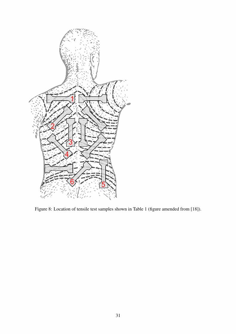
This meant that each sample had a different mean orientation and fibre dispersion. Table 1
tabulates the results of 12 different human skin samples, with different orientations, which
were procured from the backs of two different subjects2. See Fig. 8 for details of specimen
location and orientation. The preferred orientation, Θ, refers to the bisector of the two families
of fibres. The 95% Confidence Interval of the mean of these images ranged from 1.16◦−
2.77◦, thereby indicating that the preferred orientation does not change significantly over this
small area. The results of our validation revealed that the automated process differed from the
manual segmentation by an average of 5◦±4◦, giving us further confidence in the validity of
our technique.
A Pearson correlation test was carried out to test for a correlation between the measured
preferred orientation obtained through histology and the perceived orientation of Langer lines
2It should be noted here that these results have been obtained using the mle method described in Section 2.4.An alternative, but less reliable method exists whereby data is clustered into two intersecting fibre families usingan agglomerative clustering algorithm such as was performed in Nı Annaidh et al [21].
12
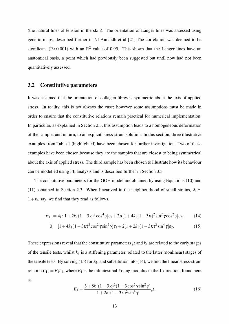
(the natural lines of tension in the skin). The orientation of Langer lines was assessed using
generic maps, described further in Nı Annaidh et al [21].The correlation was deemed to be
significant (P<0.001) with an R2 value of 0.95. This shows that the Langer lines have an
anatomical basis, a point which had previously been suggested but until now had not been
quantitatively assessed.
3.2 Constitutive parameters
It was assumed that the orientation of collagen fibres is symmetric about the axis of applied
stress. In reality, this is not always the case; however some assumptions must be made in
order to ensure that the constitutive relations remain practical for numerical implementation.
In particular, as explained in Section 2.3, this assumption leads to a homogeneous deformation
of the sample, and in turn, to an explicit stress-strain solution. In this section, three illustrative
examples from Table 1 (highlighted) have been chosen for further investigation. Two of these
examples have been chosen because they are the samples that are closest to being symmetrical
about the axis of applied stress. The third sample has been chosen to illustrate how its behaviour
can be modelled using FE analysis and is described further in Section 3.3
The constitutive parameters for the GOH model are obtained by using Equations (10) and
(11), obtained in Section 2.3. When linearized in the neighbourhood of small strains, λi '
1+ εi, say, we find that they read as follows,
σ11 = 4µ[1+2k1(1−3κ)2 cos4γ]ε1 +2µ[1+4k1(1−3κ)2 sin2
γ cos2γ]ε2, (14)
0 = [1+4k1(1−3κ)2 cos2γ sin2
γ]ε1 +2[1+2k1(1−3κ)2 sin4γ]ε2. (15)
These expressions reveal that the constitutive parameters µ and k1 are related to the early stages
of the tensile tests, whilst k2 is a stiffening parameter, related to the latter (nonlinear) stages of
the tensile tests. By solving (15) for ε2, and substitution into (14), we find the linear stress-strain
relation σ11 = E1ε1, where E1 is the infinitesimal Young modulus in the 1-direction, found here
as
E1 =3+8k1(1−3κ)2(1−3cos2 γ sin2
γ)
1+2k1(1−3κ)2 sin4γ
µ, (16)
13
(which is consistent with the formula E = 3µ in linear isotropic (κ = 1/3) incompressible
elasticity). Hence, by plotting the values of σ11 for the early part of the tests (first 1000 data
say, corresponding to a tensile stretch of less than 2%), we can determine E1 by linear regression
analysis, see Fig.9(a). Here we have plotted the ‘parallel’ sample highlighted in Table 1 data
for which was collected from tensile tests of human skin samples [21].
Once E1 is determined, µ can be expressed in terms of E1 and k1 using Eq. (16). Then the
remaining material parameters k1 and k2 are found through the nonlinear least squares fitting
with experimental test data of Equation (10), subject to the definition of λ2 in terms of λ1 given
by Equation (11). The data fitting was performed using the lsqnonlin MATLAB routine in the
Optimisation Toolbox where the objective function, Err(k), was given as
Err(k) =n
∑i=1
(yexpi − ymodel(k)
i )2 (17)
Where n is the number of experimental data points, yexpi is the experimental value and
ymodel(k)i is the value predicted by the model using the current material parameters, k.
Non-linear optimisation procedures are often sensitive to the initial starting point provided
by the user [23]. In our case, the initial estimate for k1 was found by calculating the slope
of the non-linear part of the stress-stretch curve. Since we have shown that k1 is related to
the stiffening stage of the tensile test, our initial estimate therefore has a physical meaning.
Furthermore, the initial estimates of both k1 and k2 were varied over a large range and lead to
the same set of optimal parameters each time, illustrating that the results of the optimisation
procedure are not sensitive to this initial estimate.
The results of our optimisation procedure gave us a value of 243.6 for k1 and 0.1327 for
k2, with an R2 of 99.5%. Fig.9(b) shows the GOH model fit to the experimental data. It can
be seen that these material parameters provide an excellent fitting to the ‘parallel’ sample, at
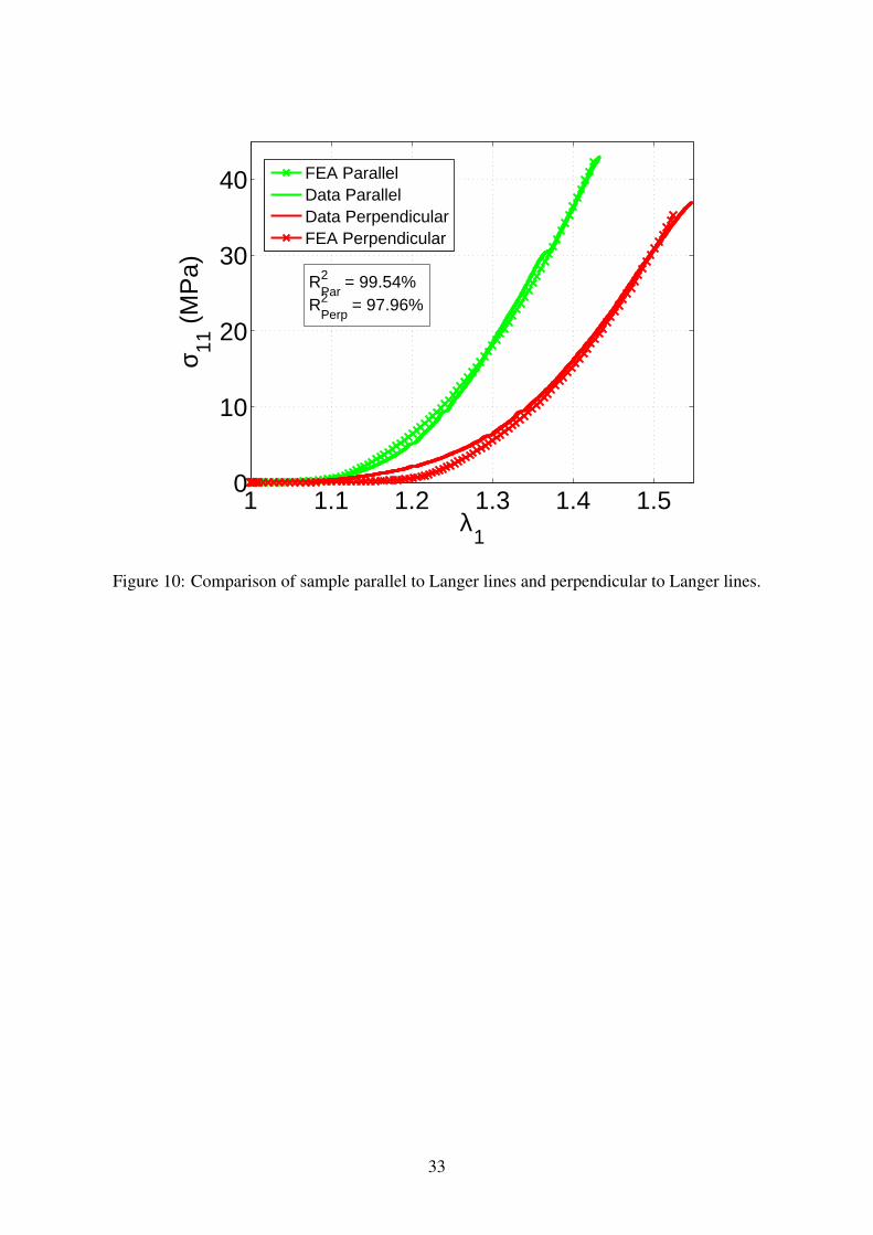
least from a descriptive point of view. Turning now to the predictive capabilities of the GOH
model, we examine a sample ‘perpendicular’ to the Langer lines. In Fig. 10 we use the material
parameters k1 and k2 obtained through least squares fitting, µ calculated by linear regression
and Eq. (16), coupled with the unique structural data for the ‘perpendicular’ sample in Table 2.
We compare the model prediction for a tensile test occurring perpendicular to the Langer lines
14

to the experimental data. The fit remains good with R2 = 97.96%. This shows that the model is
capable of predicting the behaviour of skin once the structural parameters have been evaluated.
3.3 Finite element simulations
The conventions used by ABAQUS are related to ours through C10 = µ/2, k′1 = k1µ and k′2 = k2,
so that the ABAQUS parameters used were C10 = 0.1007 MPa, k′1 = 24.53 MPa and k′2 =
0.1327.
The FE simulation results of the uniaxial tensile tests for both the parallel and perpendicular
samples were identical to the analytical solution. The results were independent of both mesh
density and element type. Fig. 11 shows the Cauchy stress distribution across the parallel and
perpendicular samples at the end of the test. The large difference in magnitudes between the
two is due to the variation in the mean orientation of fibres. Note the uniform distribution of
stress in the middle section of the test samples, thanks to the dog-bone shape of the specimen,
and the symmetry of fibres about the axis of applied stress.
As discussed in Section 3.2, for ease of determining the material parameters, it was assumed
that the orientation of collagen fibres is symmetric about the axis of applied stress. This is
for an idealised scenario only, where one knows the exact orientation of collagen fibres prior
to testing, and can therefore apply the stress in this orientation. However, with the model
parameters that have now been determined, a FE simulation can provide results for samples
where the collagen fibres are not symmetric about the axis of applied stress. Examining the non-
symmetric example in Fig. 12(a), we can see a non-uniform distribution of stress throughout the
test specimen. A local magnification of stress occurs near the neck regions of the test specimen.
This is due to the non-symmetry of collagen fibres about the axis of applied stress and makes
this problem a much more complicated one to solve analytically. The presence of significant
levels of shear in Fig. 12(b) (which is absent from both the parallel and perpendicular samples)
indicates further the effect of this non-symmetry on the sample response.
Because the stress distribution in this sample is non-uniform, to examine the predictive
capabilities of the GOH model here, we must plot the experimental force-displacement data
against the values predicted by ABAQUS for a node at the top of the test sample, see Fig. 13.
15

Again, we have found that the model predicts the behaviour well with an R2 of 94.4%, showing
that the GOH model is capable of predicting the anisotropic response of human skin.
4 Discussion
For this paper, histology slides in three different planes were examined; however, after captur-
ing the images from all three planes it was observed that three times as many cross-sectioned
fibres were present in the plane normal to the epidermis, therefore an assumption was made
to ignore the fibres normal to the epidermis. Hence, the further analysis of the samples was
restricted to the plane parallel to the epidermis alone, making this a 2D analysis. Physically
however, there are a percentage of fibres that run normal to the epidermis and this information
has not been captured here. Furthermore, unloaded collagen fibres have a crimped nature: Their
relative orientation may vary with respect to the epidermal plane. Here we have tried to over-
come this limitation by taking an average measure over six levels of depth spanning 30µm,with
the view that the general orientation of the collagen fibres are still captured. Ideally, a full 3D
analysis of the dermal structure could consider the effects of collagen crimping. A 3D analysis
was beyond the scope of this paper, but the current technique could be extended by creating a
montage of overlapping images through the thickness of the dermis, as described in Jor et al
[17], therefore turning the 2D analysis into a 3D analysis.
A further limitation of this technique is that we have assumed that the structure of the skin
biopsy removed is representative of the entire tensile test sample. In reality, the structure, and
therefore the properties of skin may vary considerably over a small area. The variation of the
mean fibre orientation over the volume of the biopsy was quantified, however, the size of the
biopsy is very small relative to the tensile test sample and we cannot infer that the variation
would be negligible. At a minimum, future studies should excise a number of biopsies along
the length of the test specimen to investigate the variation of the structure.
While this technique has been described as ‘automated’, there are still a number of ‘manual’
steps that must first be performed. The first manual task is the histological staining, combined
with the mounting of skin biopsies. The collagen detection process demands a high quality
16

of histological staining for the method to be successful and therefore, care must be taken to
follow standard procedures carefully. The second ‘manual’ task is the image acquisition phase.
Modern ‘slide scanners’ automatically scan multiple slides at once meaning that tedious image
acquisition techniques using a manual microscope are no longer necessary, however images
must still be captured from the ‘digital slide’.
While this technique has provided quantitative structural data of human skin, it can, of
course, only be applied in-vitro. Considering the effect that the mean orientation of collagen
fibres has on the mechanical response of skin, the development of in-vivo methods for establish-
ing the orientation of fibres is of the utmost importance. Advanced imaging techniques such as
ultrasonic surface wave propagation may eventually provide real-time, in-vivo structural data.
It should be noted that the nonlinear curve fitting technique rests only on measurements of
λ1 and σ11, and that λ2, along with k1 and k2 are obtained during the simultaneous optimisa-
tion of Eq. (10) and Eq. (11). Ideally, a more complete analysis would include, compare, and
contrast experimental data for λ2 and/or λ3. An extensive experimental data set would include
planar biaxial tests with in-plane shear and separate through thickness shear tests [9][15], how-
ever in the absence of these advanced testing protocols tensile tests coupled with a histological
study of the collagen fibre alignment can be used for reasonable determination of material pa-
rameters [14]. Of course non-uniqueness of optimal material parameters is an intrinsic problem
in non-linear fitting. It is possible that the optimisation procedure finds a local minimum and
assumes that this is the global minimum [23]. To ensure that the optimisation procedure is
providing a unique set of material parameters a number of checks are available: The properties
of the Hessian matrix can be investigated at the optimum [11], or alternatively, one can plot the
objective function as a function of the varying material parameters. In this case the objective
function was investigated and the plot (not reproduced) shows that our procedure calculates a
global minimum and not merely a local minimum.
In this study we have developed a simple automated process which can detect the orientation
of collagen fibres. This technique can be easily implemented in MATLAB and can be adapted
to detect other biological features, such as certain cells, leading to applications in diagnostics.
We have applied this technique to skin biopsies and provided new quantitative data on the ori-
17
entation of collagen fibres in the human dermis. So far, the availability of accurate structural
data has lagged behind the progress of anisotropic constitutive modelling. Here we have pro-
vided the structural data required to accurately make use of advances in constitutive modelling,
and help fill the void of experimental data. The model parameters of the GOH model have been
evaluated for skin using experimental data from the same skin samples. These sets of parame-
ters will provide invaluable data for those wishing to model the anisotropic behaviour of skin.
Finally, an FE simulation of a uniaxial tensile test on three separate human skin samples was
performed which predicted the the response of these three samples well. We have illustrated
that the Gasser-Ogden-Holzapfel model can successfully model the anisotropic behaviour of
human skin and that it can be implemented in ABAQUS with ease.
5 Acknowledgements
The authors acknowledge gratefully the advice and assistance of Mr. Ciaran Driver, Dr. Michael
Curtis and Prof. Marie Cassidy, of the Office of the State Pathologist (Ireland), in the area of
histology. This research was supported by a Marie Curie Intra European Fellowship within
the 7th European Community Framework Programme, awarded to MD; by the Irish Research
Council for Science, Engineering and Technology; by the Office of the State Pathologist (Irish
Department of Justice and Equality); and by the Ile-de-France region. G.S. is supported by the
PRIN 2009 project “Matematica e meccanica dei sistemi biologici e dei tessuti molli”.
References
[1] Berens, P. Circstat: A MATLAB toolbox for circular statistics. J Stat Software 31:10,
2009.
[2] Bischoff, J.E., E.M. Arruda, and K. Grosh. Finite element modeling of human skin using
an isotropic, nonlinear elastic constitutive model. J Biomech 33:645–652, 2000.
[3] Bischoff, J.E., E.M. Arruda, and K. Grosh. A rheological network model for the contin-
18
uum anisotropic and viscoelastic behaviour of soft tissue. Biomechan Model Mechanobiol
3:56–65, 2004.
[4] Cortes, D.H., S.P. Lake, J.A. Kadlowec, L.J. Soslowsky, and D.M. Elliott. Characterizing
the mechanical contribution of fiber angular distribution in connective tissue: Comparison
of two modeling approaches. Biomechan Model Mechanobiol 9:651–658, 2010.
[5] Elbischger, P., H. Bischof, P. Regitnig, and G. Holzapfel. Automatic analysis of collagen
fiber orientation in the outermost layer of human arteries. Pattern Analysis Appl 7:269–
284, 2004.
[6] Evans, S.L. On the implementation of a wrinkling, hyperelastic membrane model for skin
and other materials. Comp Meth Biomech Biomed Eng 12:319 – 332, 2009.
[7] Fisher, N. Statistical Analysis of Circular Data. Cambridge: Cambridge University Press,
1993.
[8] Flamini, V., C. Kerskens, K.M. Moerman, C.K. Simms, and C. Lally. Imaging arterial fi-
bres using diffusion tensor imaging – feasability study and preliminary results. EURASIP
J Adv Signal Proces , 2010.
[9] Flynn, C., A. Taberner and P. Nielsen. Modeling the Mechanical Response of In Vivo Hu-
man Skin Under a Rich Set of Deformations. Annals of Biomedical Engineering 39:1935-
1946, 2011.
[10] Gasser, T., R.W. Ogden, and G. Holzapfel. Hyperelastic modelling of arterial layers with
distributed collagen fibre orientations. J Roy Soc Interface 3:15–35, 2006.
[11] Gamage, T.P., V. Rajagopal, M. Ehrgott, M.P. Nash, and P.M. F. Nielsen. Identification of
mechanical properties of heterogeneous soft bodies using gravity loading. International
Journal for Numerical Methods in Biomedical Engineering 27:391-407, 2011.
[12] Haralick, R.M., and L.G. Shapiro. Computer and robot vision, vol 1. Boston, Addison-
Wesley, 1992.
19

[13] Holzapfel, G.A. Handbook of Materials Behavior Models: Biomechanics of Soft Tissue,
edited by J. Lemaitre. Academic Press, 1057-1071, 2001.
[14] Holzapfel, G.A. Determination of material models for arterial walls from uniaxial exten-
sion tests and histological structure. Journal of Theoretical Biology 238:290–302, 2006.
[15] Holzapfel, G. A. and R.W. Ogden. On planar biaxial tests for anisotropic nonlinearly
elastic solids: A continuum mechanical framework. Mathematics and Mechanics of Solids
14:474-489, 2009.
[16] Jones T.A. MATLAB functions to analyze directional (azimuthal) data–I: Single-sample
inference. Comp Geosc 32:166–175, 2006.
[17] Jor, J.W.Y., P.M.F. Nielsen, M.P. Nash, and P.J. Hunter. Modelling collagen fibre orien-
tation in porcine skin based upon confocal laser scanning microscopy. Skin Res Tech,
17:149-159, 2011.
[18] Langer, K. On the anatomy and physiology of the skin. The Imperial Academy of Science,
Vienna (1861). Reprinted in (1978): British Journal of Plastic Surgery, 17:93-106, 1978.
[19] Lanir, Y. Constitutive equations for fibrous connective tissues. J Biomech , 16:1–12.,
1983.
[20] Montagna, W. The structure and function of the skin. New York: Academic Press, 1962.
[21] Nı Annaidh, A., K. Bruyere, M. Destrade, M. Gilchrist, M. Ottenio Characterising the
anisotropic mechanical properties of excised human skin. Journal of the Mechanical Be-
haviour of Biomedical Materials. 5:139-148, 2012.
[22] Noorlander, M.L., P. Melis, A. Jonker, and C.J. Van Noorden. A quantitative method to de-
termine the orientation of collagen fibers in the dermis. J Histochem Cytochem 50:1469–
1474, 2002.
[23] Ogden, R.W., G. Saccomandi and I. Sgura. Fitting hyperelastic models to experimental
data. Computational Mechanics 34:484–502, 2004.
20
[24] Otsu, N. A threshold selection method from grey-level histograms. IEEE Trans Syst Man
Cybern. 9:62–66, 1979.
[25] Ridge, M., V. Wright. Mechanical properties of skin: A bioengineering study of skin
structure. J Appl Physiol 21:1602–1606, 1966.
[26] Ruvolo, Jr. E.C., G.N. Stamatas, and N. Kollias. Skin Viscoelasticity Displays Site- and
Age-Dependent Angular Anisotropy. Skin Pharmacol Physiol;20:313-321, 2007.
[27] Van Zuijlen, P.P.M., H.J. de Vries, E.N. Lamme, J.E. Coppens, J. Van Marle, R.W. Kries,
and E. Middelkoop. Morphometry of dermal collagen orientation by Fourier analysis is
superior to multi-observer assessment. J Pathol 198:284–291, 2002.
[28] Verhaegen, P.D.H.M., E.M. Res, A. Van Engelen, E. Middelkoop, and P.P.M. Van Zuijlen.
A reliable, non-invasive measurement tool for anisotropy in normal skin and scar tissue.
Skin research and technology 16(3):325–331, 2010.
[29] Wu, J., B. Ragwa, D. Filmer, C. Hoffmann, B. Yuan, C. Chiang, J. Sturgis, and J. Ro-
bison. Automated quantification and reconstruction of collagen matrix from 3D confocal
datasets. J Microscopy 210:158–165, 2003.
[30] Yasui, T., Y. Tohno, and T. Araki. Characterization of collagen orientation in human
dermis by two-dimensional second-harmonic-generation polarimetry. J Biomed Optics
9:259–264, 2004.
21
6 Tables & Figures
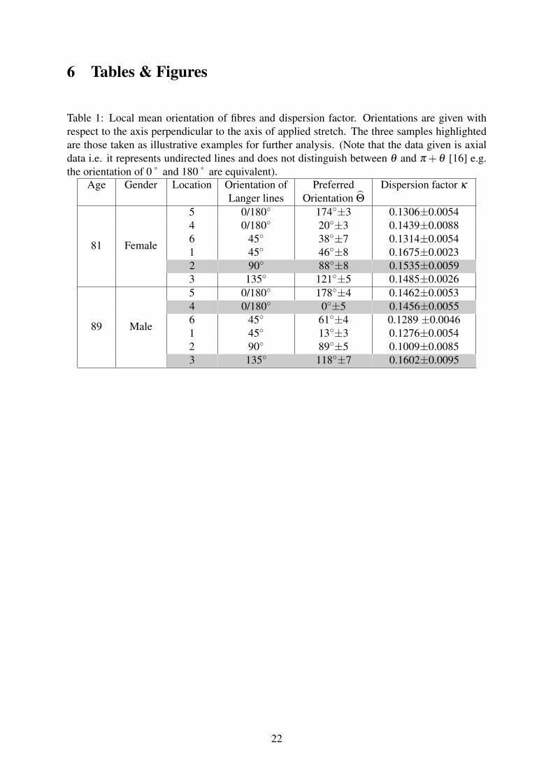
Table 1: Local mean orientation of fibres and dispersion factor. Orientations are given withrespect to the axis perpendicular to the axis of applied stretch. The three samples highlightedare those taken as illustrative examples for further analysis. (Note that the data given is axialdata i.e. it represents undirected lines and does not distinguish between θ and π +θ [16] e.g.the orientation of 0 ˚ and 180 ˚ are equivalent).
Age Gender Location Orientation ofLanger lines
PreferredOrientation Θ
Dispersion factor κ
81 Female
5 0/180◦ 174◦±3 0.1306±0.00544 0/180◦ 20◦±3 0.1439±0.00886 45◦ 38◦±7 0.1314±0.00541 45◦ 46◦±8 0.1675±0.00232 90◦ 88◦±8 0.1535±0.00593 135◦ 121◦±5 0.1485±0.0026
89 Male
5 0/180◦ 178◦±4 0.1462±0.00534 0/180◦ 0◦±5 0.1456±0.00556 45◦ 61◦±4 0.1289 ±0.00461 45◦ 13◦±3 0.1276±0.00542 90◦ 89◦±5 0.1009±0.00853 135◦ 118◦±7 0.1602±0.0095
22
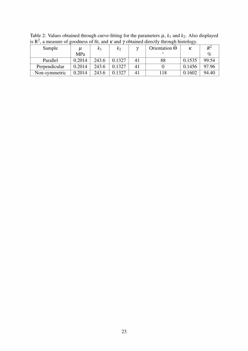
Table 2: Values obtained through curve-fitting for the parameters µ , k1 and k2. Also displayedis R2, a measure of goodness of fit, and κ and γ obtained directly through histology.
Sample µ k1 k2 γ Orientation Θ κ R2
MPa ◦ %Parallel 0.2014 243.6 0.1327 41 88 0.1535 99.54
Perpendicular 0.2014 243.6 0.1327 41 0 0.1456 97.96Non-symmetric 0.2014 243.6 0.1327 41 118 0.1602 94.40
23
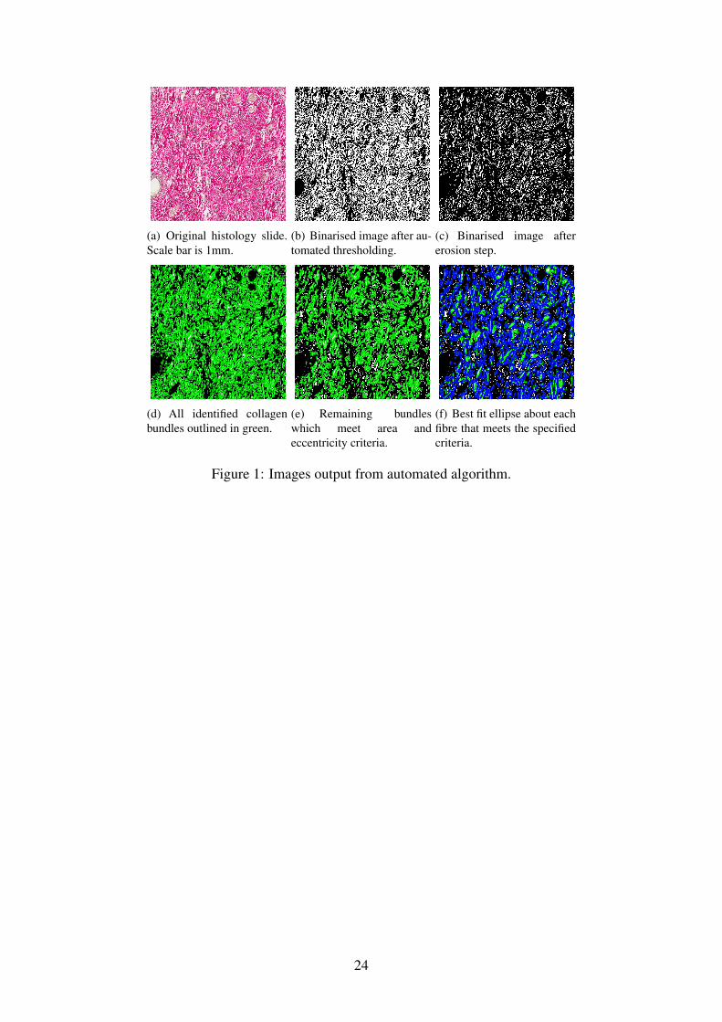
(a) Original histology slide.Scale bar is 1mm.
(b) Binarised image after au-tomated thresholding.
(c) Binarised image aftererosion step.
(d) All identified collagenbundles outlined in green.
(e) Remaining bundleswhich meet area andeccentricity criteria.
(f) Best fit ellipse about eachfibre that meets the specifiedcriteria.
Figure 1: Images output from automated algorithm.
24

0 100 200 3000
0.01
0.02
0.03
0.04
Orientation (θ)
p, P
roba
bilit
y D
ensi
ty
2γ
Figure 2: Histogram of collagen orientations. The two distinct peaks correspond to the pre-ferred orientation of the two fiber families. The angle, γ , is half the distance between the twopeaks i.e. γ=41◦.
25

Figure 3: Lattice structure of crossing collagen fibres with fibre dispersion taken into account.
26
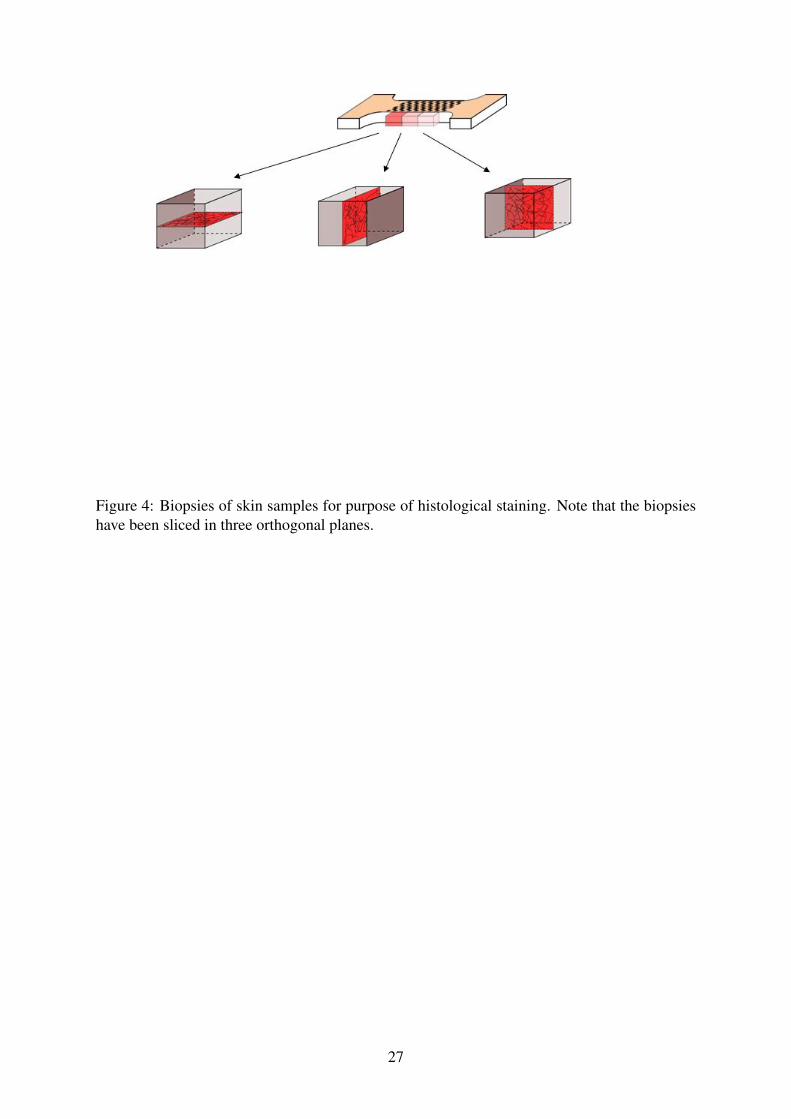
Figure 4: Biopsies of skin samples for purpose of histological staining. Note that the biopsieshave been sliced in three orthogonal planes.
27

Figure 5: Manual segmentation of collagen. Elongated fibres were marked by black lines, andtheir orientation was later measured manually.
28
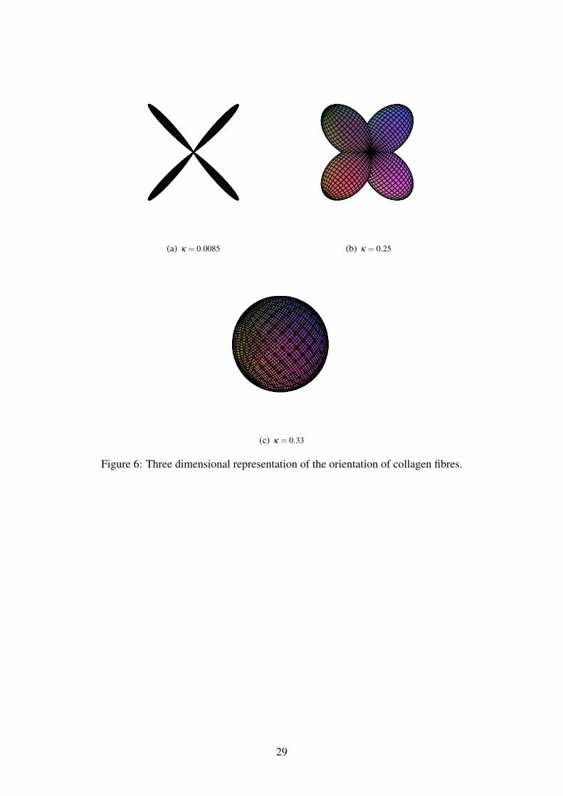
(a) κ = 0.0085 (b) κ = 0.25
(c) κ = 0.33
Figure 6: Three dimensional representation of the orientation of collagen fibres.
29
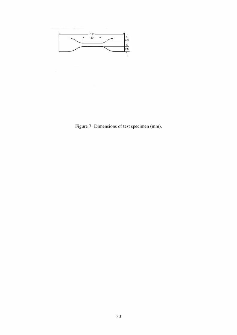
Figure 7: Dimensions of test specimen (mm).
30
1
2
3
4
56
Figure 8: Location of tensile test samples shown in Table 1 (figure amended from [18]).
31

1 1.005 1.01 1.015 1.02−0.01
0
0.01
0.02
0.03
0.04
λ1
σ 11 (
MP
a)
Data Linear
(a)
1 1.1 1.2 1.3 1.40
10
20
30
40
λ1
σ 11 (
MP
a)
SlopeExp DataGOH Model
(b)
Figure 9: Nonlinear curve fitting to obtain the constitutive parameters: µ and k1 are related tothe early (infinitesimal) stress-strain part of the graph, see (a); k2, to the rest of the curve.
32
1 1.1 1.2 1.3 1.4 1.50
10
20
30
40
λ1
σ 11 (
MP
a)
FEA ParallelData ParallelData PerpendicularFEA Perpendicular
R2Par
= 99.54%R2
Perp = 97.96%
Figure 10: Comparison of sample parallel to Langer lines and perpendicular to Langer lines.
33

(Avg: 75%)
S, S11
+3.210e+06+8.176e+06+1.314e+07+1.811e+07+2.308e+07+2.804e+07+3.301e+07+3.797e+07+4.294e+07+4.791e+07+5.287e+07+5.784e+07+6.281e+07
(a) (b)
Figure 11: Cauchy stress in Pa of sample strained by 50% (a) Parallel to the Langer lines (b)Perpendicular to the Langer lines.
34

(Avg: 75%)
S, S11
+1.131e+05+5.632e+06+1.115e+07+1.667e+07+2.219e+07+2.771e+07+3.323e+07+3.875e+07+4.426e+07+4.978e+07+5.530e+07+6.082e+07+6.634e+07
(a)
(Avg: 75%)
S, S12
−7.213e+06−4.916e+06−2.620e+06−3.231e+05+1.973e+06+4.270e+06+6.566e+06+8.863e+06+1.116e+07+1.346e+07+1.575e+07+1.805e+07+2.035e+07
(b)
Figure 12: Cauchy stress in Pa of a non-symmetric sample strained by 30% (a) σ11 (b) σ12
35

0 5 10 15 200
100
200
300
400
Displacement (mm)
For
ce (
N)
FEAData
R2 = 94.4%
Figure 13: Comparison between predicted model response and experimental force-displacement data for a non-symmetric sample.
36