Embed Size (px)
Citation preview
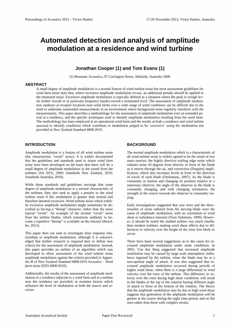
Proceedings of Acoustics 2013 – Victor Harbor 17-20 November 2013, Victor Harbor, Australia
Australian Acoustical Society 1
Automated detection and analysis of amplitude modulation at a residence and wind turbine
Jonathan Cooper (1) and Tom Evans (1)
(1) Resonate Acoustics, 97 Carrington Street, Adelaide, Australia 5000
ABSTRACT A small degree of amplitude modulation is a normal feature of wind turbine noise but most assessment guidelines for
wind farm noise state that, where excessive amplitude modulation occurs, an additional penalty should be applied to
the measured noise. Excessive amplitude modulation is typically defined as a situation where the peak to trough lev-
els (either overall or in particular frequency bands) exceed a nominated level. The assessment of amplitude modula-
tion outdoors at receptor locations near wind farms over a wide range of wind conditions can be difficult due to the
need to undertake unattended measurements in an environment where background noise regularly interferes with the
measurements. This paper describes a methodology for the assessment of amplitude modulation over an extended pe-
riod at a residence, and the specific techniques used to identify amplitude modulation resulting from the wind farm.
The methodology has been employed at an operational wind farm and the results at both a residence and wind turbine
assessed to identify conditions which contribute to modulation judged to be ‘excessive’ using the modulation test
provided in New Zealand Standard 6808:2010.
INTRODUCTION
Amplitude modulation is a feature of all wind turbine noise
(the characteristic “swish” noise). It is widely documented
that the guidelines and standards used to assess wind farm
noise have been developed on the basis that there will be a
small degree of amplitude modulation in the sound from the
turbines (SA EPA, 2009; Standards New Zealand, 2010;
Standards Australia, 2010).
While these standards and guidelines envisage that some
degree of amplitude modulation is a normal characteristic of
the turbines, they also seek to apply a penalty to the wind
turbine noise if this modulation is greater than normal and
therefore deemed excessive. Wind turbine noise which exhib-
its excessive amplitude modulation might sometimes be de-
scribed as having a “thump” character, rather than the more
typical “swish”. An example of the normal “swish” noise
from the turbine blades, which transitions suddenly to be-
come a repetitive “thump” is available on the internet (Bowd-
ler, 2013).
This paper does not seek to investigate dose response rela-
tionships to amplitude modulation, although it is acknowl-
edged that further research is required here to define new
criteria for the assessment of amplitude modulation. Instead,
this paper provides an outline of an algorithm which was
developed to allow assessment of the wind turbine noise
amplitude modulation against the criteria provided in Appen-
dix B of New Zealand Standard 6808:2010 Acoustics – Wind
farm noise (NZS 6808:2010).
Additionally, the results of the assessment of amplitude mod-
ulation at a residence adjacent to a wind farm and at a turbine
near the residence are provided, to examine factors which
influence the level of modulation at both the source and re-
ceiver.
BACKGROUND
The normal amplitude modulation which is a characteristic of
all wind turbine noise is widely agreed to be the result of two
main sources; the highly directive trailing edge noise which
radiates noise 45 degrees from directly in front of the blade
as it moves through the air, and convective (Doppler) ampli-
fication, which also increases levels in front of the direction
of travel of each blade (Oerlemans, 2007). As the blade is
constantly in motion and changing its position relative to a
stationary observer, the angle of the observer to the blade is
constantly changing, and with changing orientation, the
strength of the source towards the observer is constantly var-
ying.
Early investigations suggested that yaw error and the direc-
tionality of noise radiated from the moving blade were the
cause of amplitude modulation, with no correlation to wind
shear or turbulence intensity (Flow Solutions, 1999). Howev-
er, it should be noted the studied turbine was much smaller
than modern turbines, making wind shear effects due to dif-
ferences in velocity over the height of the rotor less likely to
occur.
There have been several suggestions as to the cause for in-
creased amplitude modulation under some conditions. In
2003, Van den Berg suggested that increased amplitude
modulation may be caused by large scale atmospheric turbu-
lence ingested by the turbine, when the blade may be at a
non-optimal angle of attack. It was also suggested that in-
creased amplitude modulation occurred during periods of
higher wind shear, when there is a large differential in wind
velocity over the rotor of the turbine. This difference in ve-
locity over the rotor during high shear conditions will result
in the blades at the top of the rotation having different angle
of attack to those at the bottom of the rotation. The theory
that the amplitude modulation may be due to high wind shear
suggests that generation of the amplitude modulation will be
greater at the source during the night time period, and on flat
sites rather than those with complex terrain.
Paper Peer Reviewed
Proceedings of Acoustics 2013 – Victor Harbor 17-20 November 2013, Victor Harbor, Australia
2 Australian Acoustical Society
Amplitude modulation is currently the focus of a large body
of research being funded by RenewableUK (Cand, 2012).
One part of that work is to investigate causes of amplitude
modulation, and a summary of the causes of both normal and
excessive amplitude modulation was provided by the re-
search group last year (Smith, 2012). They suggest that the
non-uniform flow over the rotor of the turbine (due to either a
wind gust or wind shear) is a likely cause of excessive ampli-
tude modulation, but note that propagation effects due to the
change in height of the source may also contribute to exces-
sive amplitude modulation upwind of the turbines.
ASSESSMENT CRITERIA
This paper focuses on the assessment of amplitude modula-
tion against the requirements of NZS 6808:2010. As the
South Australian Wind farms environmental noise guidelines
(SA EPA, 2009) and Australian Standard AS 4959 (Stand-
ards Australia, 2010) do not provide specific criteria for ex-
cessive amplitude modulation, NZS 6808:2010 is the only
finalised assessment document used in Australia that does.
Section B3.2 of Appendix B of NZS 6808:2010 states the
following with regards to the assessment of amplitude modu-
lation: …. modulation special audible characteristics are
deemed to exist if the measured A-weighted peak
to trough levels exceed 5 dB on a regularly varying basis, or if the measured third-octave band peak to
trough levels exceed 6 dB on a regular basis in re-
spect of the blade pass frequency.
A draft guideline document for the assessment of wind farm
noise was prepared by the Environment Protection Authority
Victoria (EPA Victoria) and circulated for information and
comment to members of the Australian Acoustical Society.
That draft document provides further information on how the
test in NZS 6808:2010 should be applied in Victoria: The interim test method specifies peak to trough level differences in respect of the blade pass fre-
quency. The blade pass frequency should be meas-
ured directly from the rotational speed of the wind turbine during sound level measurements under the
interim test method. The rotational speed/blade
pass frequency may vary during the measurements and the analysis should be for the specific blade
pass frequency at all times. The peak to trough lev-
el difference should only be determined for adja-cent peaks and troughs at this varying frequency.
The test method requires the peak to trough level differences to be occurring regularly. For this guide
the average level difference should be taken over a
2 minute time period. If the level difference thresh-olds are exceeded within any 2 minute period with-
in a 10 minute measurement, then the +5 dB ad-
justment should be applied to that wind farm sound level LA90(10 min).
A 5 dB adjustment is applied to the individual LA90,10 min pe-
riods in which amplitude modulation is found to exceed the
5 dB A-weighted or 6 dB third octave peak to trough criteria
in any 2-minute period in that measurement.
METHODS FOR ASSESSING MODULATION
Two methods have previously been used for calculating the
level of amplitude modulation. The first, and easiest method
to apply, uses the simple visual examination of the time se-
ries (typically sampled at 100 ms time intervals) to pick off
the local maxima and minima. The level of amplitude modu-
lation is then calculated as average difference between the
maxima and minima. This method is easy to apply for a short
measurement (for example 2 minutes), but impractical when
the analysis seeks to identify the level of amplitude modula-
tion continuously over days or weeks at a wind farm site.
The second method that has been previously used to calculate
the level of amplitude modulation uses more intensive signal
analysis to determine the RMS level of modulation. This is
normally achieved using one of the following methods:
Double application of a spectrum analysis to a measured
signal. The first spectrum analysis is used to provide
short time series levels (typically 100 ms levels) as ei-
ther an overall A-weighted level or in third octave bands
(analysis potentially undertaken in real time on the
sound level meter). A power spectrum is then taken of
the 100 ms data, to calculate the frequency of modula-
tion and level of the amplitude modulation (Lee, 2009).
The raw audio signal is band filtered into third octave
bands, and a Hilbert transform used to calculate the sig-
nals envelope. A power spectrum is then taken of the
band limited enveloped signal, to determine the modula-
tion frequency and level in that band (McCabe, 2011).
The advantage of the more intensive signal analysis tech-
niques is that they can be used to automatically calculate the
level of amplitude modulation during long-term measure-
ments of several weeks duration. The disadvantage of these
methods is the susceptibility to extraneous noise, which may
be falsely identified as amplitude modulation, or may make
identification of the level of amplitude modulation due to the
wind farm noise indistinguishable from other sources.
The more intensive methods also determine the RMS level of
amplitude modulation, rather than a peak to trough level like
the visual inspection. In practice, the blade pass modulation
is not a perfect sine wave in shape, so RMS assessment tech-
niques cannot be used to determine amplitude modulation for
assessment against a peak to trough criterion as required by
NZS 6808:2010. RMS assessments could be used to deter-
mine the level of modulation against a RMS modulation cri-
terion, but these criteria for wind turbine noise do not exist at
the present time. One aim of the work being undertaken for
RenewableUK was the development of the dose response
relationship for the RMS level of modulation for wind tur-
bine noise (Cand, 2012).
IMPLEMENTATION OF A HYBRID METHOD
To allow the assessment of amplitude modulation against the
criteria contained in Appendix B of NZS 6808:2010 over an
extended period of time, a hybrid method was developed.
This method uses frequency analysis to find the frequency of
blade pass modulation, and then a peak finding algorithm to
identify individual peaks and troughs, and therefore the dif-
ference in level for each blade pass. The frequency analysis
to find the blade pass frequency was on 100 ms third octave
band results rather than an envelope of an audio signal as
NZS 6808:2010 requires the use of 100 ms third octave re-
sults for calculating the modulation depth.
The amplitude modulation detection algorithm allowed the
automated detection of amplitude modulation in both the A-
weighted and one-third octave band data at the residence for
a dataset of several weeks duration.
The third octave and A-weighted data required for the as-
sessment of amplitude modulation in accordance with NZS
6808:2010 was gathered in 100 ms intervals using a SVAN
979 sound level meter. Audio data was stored for the full
Proceedings of Acoustics 2013 – Victor Harbor 17-20 November 2013, Victor Harbor, Australia
Australian Acoustical Society 3
duration of the measurements on a second adjacent sound
level meter, which allowed review of the source of the ampli-
tude modulation if the average level of modulation during a
two-minute period exceeded the modulation criteria.
Rotational speed data was initially sourced from the nearest
turbines to the residence, as directed by the draft guideline
document developed by EPA Victoria. However, review of
the results of the assessment indicated that it was not possible
to find a turbine, or group of turbines where the rotational
speed of the turbines was consistently representative of the
rate of blade pass modulation at the residence. There were
times when blade pass was audible at the residence when the
nearest turbines were not operating (showing 0 rotational
speed), but other periods when the modulation was controlled
by the nearest turbines. Additionally, rotational speed data
was available as only average speeds in 10-minute periods,
with changes in speed throughout the period not recorded.
Identification of blade pass frequency bands
The first step in the implementation of an automated blade
pass identification algorithm was to determine the modula-
tion frequency of the wind turbine noise in each 2 minute
measurement period. As indicated above, the rotational speed
data sourced from the turbines was not found to provide a
reliable indicator of the modulation frequency.
To use the data stored in 100 ms intervals at the residence to
find the blade pass frequency, it was necessary to identify the
frequency bands (third octave bands and/or A-weighted, C-
weighted and Linear levels) in which blade pass modulation
could be regularly detected.
The power spectrum of the 100 ms sound pressure levels
(measured in dB) in all third octave, overall A-weighted,
overall C-weighted and overall Linear bands was calculated,
to identify repetitive patterns and hopefully therefore blade
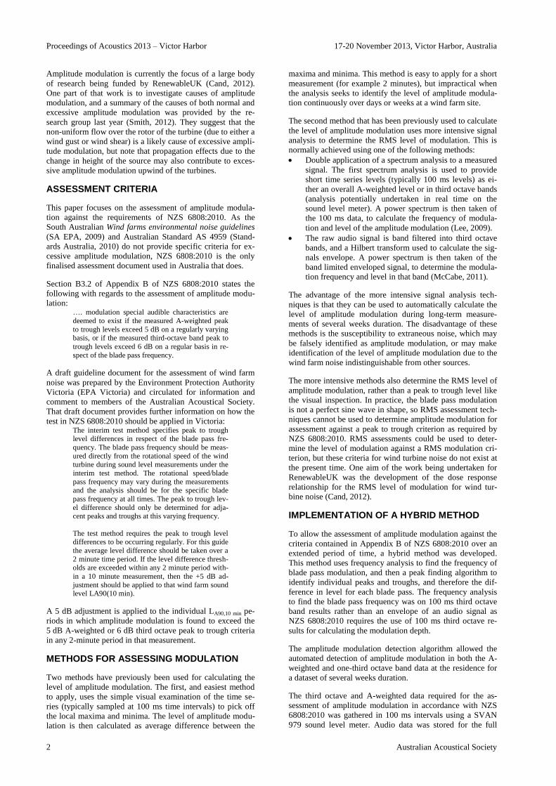
pass in each of the bands. Figure 1 shows a simple example
when there is very little extraneous noise and blade pass
modulation occurring in the 100ms overall A-weighted noise
level stored over the majority of a 2 minute period at the
residence. The modulation is particularly clear during the
first half of the measurement. The power spectrum of the
100ms data in dB presented in Figure 1 is included as Figure
2, calculated using a Hanning window with 50% overlap and
resolution of 0.05 Hz.
32
36
40
44
0 100 200 300 400 500 600 700 800 900 1000 1100 1200
Sou
nd
Pre
ssu
re L
eve
l (d
B(A
))
100ms sample number
Measurement Period #1
Figure 1. Blade pass modulation visible in the overall A-
weighted 100 ms measurements over a 2 minute period.
The significant peak on the graph in Figure 2 indicates the
modulation frequency of the 100 ms noise levels presented in
Figure 1 to be 0.65 Hz. The peak to trough level of the modu-
lation (based on the false assumption of perfect sine wave
modulation) would be calculated by multiplying the square
root of the peak at 0.65 Hz by 2√2, as the peak to peak level
of any sinusoidal wave is 2√2 times the RMS level.
0
0.05
0.1
0.15
0.2
0.25
0.3
0.35
0 0.5 1 1.5 2 2.5 3 3.5 4
Po
we
r Sp
ect
rum
leve
l (d
B^2
)
Modulation frequency (Hz)
Modulation frequency of Period #1
Figure 2. Power spectrum result of the 100 ms data presented
in Figure 1, which shows the blade pass modulation frequen-
cy to be 0.65 Hz.
As the turbine noise in all frequency bands is due to the rota-
tion of the turbine blades, the modulation frequency in all
frequency bands will be the same. It is therefore not neces-
sary to correctly identify the blade pass frequency in every
individual frequency band, but rather is possible to identify
the blade pass frequency on results in all the other frequency
bands in the same 2 minute period. The blade pass frequency
for a 2 minute period could then be identified by taking the
most commonly detected modulation frequency in all fre-
quency bands during the 2 minute period.
Review of the blade pass frequency selected from power
spectrums of all third octave bands between 0.8 Hz and
20 kHz octaves indicated that under conditions when the
turbine noise was controlling the noise level at the residence,
the blade pass frequency could occasionally be detected in all
third octaves between approximately 50 Hz and 2500 Hz, and
also in the A- and C-weighted levels. However, reliable de-
tection of the blade pass frequency was rare, and was not
immediately obvious from the inspection of the power spec-
trums of all the frequency bands in about 90% of the 2 mi-
nute assessment periods at the residence.
During the initial stages of development of the blade pass
frequency detection algorithm the third octave bands between
200 Hz and 1250 Hz, and the C-weighted level were used to
try and identify the blade pass frequency, as under good con-
ditions the blade pass frequency was more obvious in these
frequency bands. It was suspected that the use of a broad
range of frequency bands would reduce the chance of an
extraneous modulating noise source controlling noise levels
in the majority of the bands, and therefore improve detection
of blade pass modulation during periods of extraneous noise.
However, it was later found the most reliable detection of
blade pass frequency was achieved using only the 250 Hz to
1000 Hz third octave bands.
The power spectrum of the 100 ms A-weighted level was not
a particularly reliable indicator of the blade pass frequency
for the majority of the measurements at the residence due to
its sensitivity to noise in the 1000 Hz to 4000 Hz frequency
range; where modulated bird, insect and other animal calls
(such as frogs) are frequent.
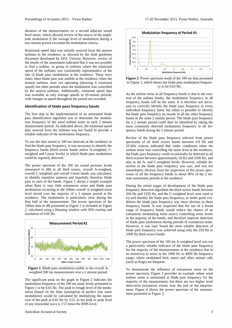
To demonstrate the influence of extraneous noise on the
power spectrum, Figure 3 provides an example where wind
turbine noise is modulated at blade pass frequency for the
majority of the measurement, but there are two higher level
short-term extraneous events near the end of the measure-
ment. Figure 4 shows the power spectrum of the measure-
ment presented in Figure 3.
Proceedings of Acoustics 2013 – Victor Harbor 17-20 November 2013, Victor Harbor, Australia
4 Australian Acoustical Society
32
36
40
44
48
52
56
60
64
0 100 200 300 400 500 600 700 800 900 1000 1100 1200
Sou
nd
Pre
ssu
re L
eve
l (d
B(A
))
100ms sample number
Measurement Period #2
Figure 3. Blade pass modulation visible in A-weighted
100 ms measurements over a 2 minute period, with two high
level extraneous events at the end of the measurement.
0
0.05
0.1
0.15
0.2
0.25
0.3
0.35
0.4
0.45
0 0.5 1 1.5 2 2.5 3 3.5 4
Po
we
r Sp
ect
rum
leve
l (d
B^2
)
Modulation frequency (Hz)
Modulation frequency of Period #2
Figure 4. Power Spectrum of the 100 ms data presented in
Figure 3, with modulation due to the two high level extrane-
ous events apparent, along with multiple harmonics.
Figure 4 provides a less clear indication of the modulation
frequency than the power spectrum in Figure 2, as the two
extraneous events spaced 2.4 seconds apart have resulted in
the power spectrum showing amplitude modulation at ap-
proximately 0.4 Hz (1 / 2.4 seconds). Multiple high level
harmonics of the 0.4 Hz peak are also visible, along with the
peak due to the actual modulation of the wind farm noise at
0.65 Hz. The possible wind turbine operational speeds in-
cluded 0.4 Hz, and so selection of the highest peak in the
operational range of the turbine would have resulted in mis-
taken identification of the blade pass frequency.
From review of a large number of turbine and non-turbine
controlled measurements, it was apparent that modulation
due to the wind turbine did not show harmonics at nearly the
same high level as the harmonics due to two (or more) close-
ly spaced extraneous events. On this basis a test was imple-
mented to sort through the peaks showing possible blade pass
frequency, and discard peaks with high level second or third
harmonics until a likely turbine blade pass frequency was
found. Where no possible peak passed the second and third
harmonic level test, a tone passing only the second harmonic
test was selected. Where no peak passed either test, the high-
est level peak was selected.
Further improvements in finding the blade pass frequency
A number of additional improvements in the identification of
the blade pass frequency were implemented. The first and
most significant improvement was to identify the modulation
frequency in each individual FFT window of each third oc-
tave band, rather than using the average 2 minute power
spectrum for each third octave band. The relationship be-
tween frequency resolution (filter bandwidth, B (Hz)) and
length of the individual window (sample time, T (seconds)) is
given by Equation (1).
B = 1 / T (1)
As a compromise between maintaining reasonable frequency
resolution while trying to maximise the number of individual
windows in a 2 minute period, a sample time for each indi-
vidual window of 24 seconds was selected. This gives a blade
pass frequency resolution of about 0.042 Hz, and with a 50%
window overlap allows nine individual 24 second long power
spectrums to be calculated in each 2-minute period for each
of the third octave bands.
Taking the measurement in Figure 3 as an example, the mod-
ulation frequency calculated from the first eight windows
would have correctly identified the blade pass frequency,
while the ninth window (on the last 24 seconds in the meas-
urement period) will identify the modulation frequency based
on the spacing between the two extraneous peaks.
The algorithm uses the result from nine FFT windows in each
of the seven frequency bands (the number of third octave
bands between 250 Hz and 1000 Hz inclusive), so that 63
power spectrums are used to identify the modulation frequen-
cy in every 2-minute period. Falsely identified modulation
frequencies due to extraneous noise are typically randomly
distributed throughout the possible frequency range, while
the blade pass frequency is correctly identified during quieter
periods in any of the third octave bands.
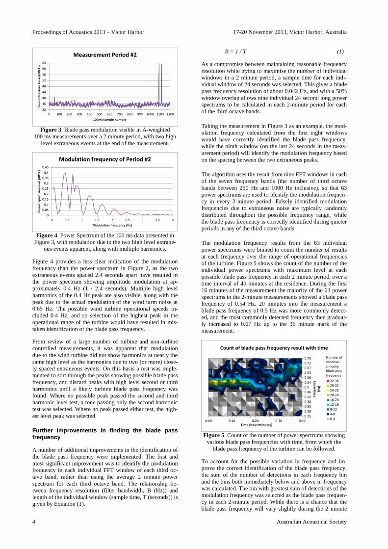
The modulation frequency results from the 63 individual
power spectrums were binned to count the number of results
at each frequency over the range of operational frequencies
of the turbine. Figure 5 shows the count of the number of the
individual power spectrums with maximum level at each
possible blade pass frequency in each 2 minute period, over a
time interval of 40 minutes at the residence. During the first
16 minutes of the measurement the majority of the 63 power
spectrums in the 2-minute measurements showed a blade pass
frequency of 0.54 Hz. 20 minutes into the measurement a
blade pass frequency of 0.5 Hz was more commonly detect-
ed, and the most commonly detected frequency then gradual-
ly increased to 0.67 Hz up to the 36 minute mark of the
measurement.
0.25
0.29
0.33
0.38
0.42
0.46
0.5
0.54
0.58
0.63
0.67
0.71
0.75
0:00 0:10 0:20 0:30 0:40
Fre
qu
en
cy
(Hz)
Time (hour:minutes)
Count of blade pass frequency result with time
32-36
28-32
24-28
20-24
16-20
12-16
8-12
4-8
0-4
Number of windowsshowing blade pass frequency
Figure 5. Count of the number of power spectrums showing
various blade pass frequencies with time, from which the
blade pass frequency of the turbine can be followed.
To account for the possible variation in frequency and im-
prove the correct identification of the blade pass frequency,
the sum of the number of detections in each frequency bin
and the bins both immediately below and above in frequency
was calculated. The bin with greatest sum of detections of the
modulation frequency was selected as the blade pass frequen-
cy in each 2-minute period. While there is a chance that the
blade pass frequency will vary slightly during the 2 minute

Proceedings of Acoustics 2013 – Victor Harbor 17-20 November 2013, Victor Harbor, Australia
Australian Acoustical Society 5
measurement, an analysis of frequency variation showed it
was relatively rare for this to be more than the frequency
resolution (0.0417 Hz) and never more than twice the fre-
quency resolution (0.0833 Hz). Any variation in blade pass
will therefore be captured in a sum of three adjacent bands.
The 40 minute period presented in Figure 5 shows the num-
ber of detections of each frequency during a time with rela-
tively little extraneous noise, particularly during the first
20 minutes of that measurement. The influence of extraneous
noise made identification of the blade pass frequency more
difficult than the example presented for the majority of the
measurements.
The lack of large variation in blade pass frequency with time
was able to be used to improve the accuracy of the blade pass
frequency detection in periods of significant extraneous
noise, by preferentially weighting the counts in frequency
bins nearer to the blade pass frequency in the previous
2-minute period. Counts in the frequency bin matching the
blade pass of the previous 2 minute period were assigned a
weighting of 1, with the weighting applied to every other bin
calculated as per Equation 2, where W is the weighting ap-
plied to the count in that frequency bin and N is the number
of frequency bins between the previous blade pass frequency
bin and the frequency of that band.
W = 1 – 0.1*N (2)
Figure 6 provides the count of the number of individual pow-
er spectrums indicating blade pass at each possible frequen-
cy, over a 40 minute period with significant extraneous mask-
ing noise at the residence. Figure 7 shows the same 40 minute
period, but with preferential weighting to the blade pass fre-
quency in the previous 2 minute period applied. From a com-
parison of Figures 6 and 7, the blade pass frequency is more
easily identified with the preferential weighting applied.
0.25
0.29
0.33
0.38
0.42
0.46
0.5
0.54
0.58
0.63
0.67
0.71
0.75
0:00 0:10 0:20 0:30 0:40
Fre
qu
en
cy
(Hz)
Time (hour:minutes)
Count of blade pass frequency with time
16-18
14-16
12-14
10-12
8-10
6-8
4-6
2-4
0-2
Number of windowsshowing blade pass frequency
Figure 6. Count of the number of power spectrums showing
blade pass frequency during a period of significant extrane-
ous noise.
The improvements to the blade pass frequency analysis pro-
vided significantly more reliable detection of the blade pass
frequency than provided from a single power spectrum of the
2 minute period. However, there were periods when the fre-
quency of the blade pass was unable to be determined due to
the significant extraneous noise present for that period.
0.25
0.29
0.33
0.38
0.42
0.46
0.5
0.54
0.58
0.63
0.67
0.71
0.75
0:00 0:10 0:20 0:30 0:40
Fre
qu
en
cy
(Hz)
Time (hour:minutes)
Count of blade pass frequency with time -weighted to previously detected frequency
16-18
14-16
12-14
10-12
8-10
6-8
4-6
2-4
0-2
Number of windowsshowing blade pass frequency
Figure 7. Count of the number of power spectrums showing
blade pass frequency during a period of significant extrane-
ous noise, but with weighting applied to favour the blade pass
frequency identified in the previous 2 minute period.
The final measure implemented to allow the blade pass fre-
quency to be determined at the residence was to restrict the
allowable change in blade pass frequency between adjacent
2 minute periods. In the case that the change in frequency
was less than or equal to one frequency bin, the change was
followed. If the change was greater than one frequency bin
but less than or equal to 2 frequency bins, it was more likely
that this change was due to extraneous noise, and the adopted
change was 1/3rd of the difference. When the change in fre-
quency was greater than two frequency bins, it was clearly
not due to actual blade pass noise and a change of 1/3rd of the
frequency resolution was applied. The approach adopted
meant that a realistic change in frequency was followed, but
the change due to an extraneous source would not significant-
ly alter the blade pass frequency, and would be recovered by
the next correct frequency detection. Blade pass frequencies
very different to the frequency of the previous 2 minute peri-
od were not ignored, so that the blade pass frequency would
be automatically re-acquired by the algorithm if lost due to
long term extraneous amplitude modulation or the shutdown
of the turbines.
A review of the results of the blade pass detection against a
number of manually calculated periods throughout the as-
sessment period at the house indicated the blade pass fre-
quency was being correctly identified whenever turbine blade
pass noise was audible. The blade pass frequency was able to
be correctly identified whenever modulation was identified
through visible inspection of the 100 ms measurement series.
The review of the results also found that the modulation fre-
quency of the wind turbine noise was being calculated signif-
icantly more reliably using the above method than the ap-
proach of adopting the operational speed of one or more of
the nearest turbines to the residence.
Calculation of level of modulation
It was relatively easy to automatically calculate the average
peak to trough level once the blade pass frequency had been
determined.
The blade pass frequency determined for each 2-minute peri-
od was first used to calculate the expected number of 100 ms
samples between each blade pass. As an example, for a 0.5
Hz blade pass frequency, the local maxima would be ex-
pected to be spaced 1/0.5 = 2 seconds, or twenty 100 ms
samples apart.
Proceedings of Acoustics 2013 – Victor Harbor 17-20 November 2013, Victor Harbor, Australia
6 Australian Acoustical Society
It was noted that while the spacing between each broad peak
due to blade pass was relatively regular, the 100 ms levels did
not follow a perfect sine wave and the broad peaks and
troughs were irregularly shaped. For this reason the spacing
between the 100 ms samples containing maxima and minima
was somewhat irregular.
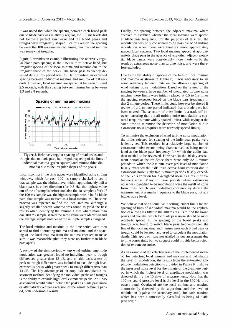
Figure 8 provides an example illustrating the relatively regu-
lar blade pass spacing in the 315 Hz third octave band, but
irregular spacing of the local minima and maxima due to the
irregular shape of the peaks. The blade pass frequency de-
tected during this period was 0.5 Hz, providing an expected
spacing between individual maxima and minima of 2.0 sec-
onds. However, local maxima are spaced at between 1.5 and
2.5 seconds, with the spacing between minima being between
1.3 and 2.8 seconds.
0
5
10
15
20
25
30
0:00 0:05 0:10 0:15 0:20
Sou
nd
pre
ssu
re le
vel (
dB
)
Time (minutes:seconds)
Spacing of minima and maxima
100 ms Lp local minima local maxima
Figure 8. Relatively regular spacing of broad peaks and
troughs due to blade pass, but irregular spacing of the lines of
individual maxima (green squares) and minima (blue dia-
monds) due to the irregular shapes of the peaks.
Local maxima in the time traces were identified using sliding
windows, which for each 100 ms sample checked to see if
that sample was the highest level within approximately half a
blade pass in either direction (for 0.5 Hz, the highest value
out of the 10 samples before and also the 10 samples after). If
the 100 ms sample was the highest sample within half a blade
pass, that sample was marked as a local maximum. The same
process was repeated to find the local minima, although a
slightly smaller search window was found to yield the best
results when identifying the minima. Cases where more than
one 100 ms sample shared the same value were identified and
the average sample number of the multiple samples assigned.
The local minima and maxima in the time series were then
sorted to find alternating minima and maxima, and the spac-
ing of the local maxima from the minima checked to make
sure it was reasonable (that they were no further than blade
pass apart).
A review of the time periods where wind turbine amplitude
modulation was greatest found no individual peak to trough
differences greater than 13 dB, and on this basis a test of
peak to trough differences was included to exclude high level
extraneous peaks with greater peak to trough differences than
13 dB. The key advantage of an amplitude modulation as-
sessment method identifying the individual peaks and troughs
is the ability to exclude high level extraneous peaks. An RMS
assessment would either include the peaks as blade pass noise
or alternatively require exclusion of the whole 2-minute peri-
od, both undesirable results.
Finally, the spacing between the adjacent maxima where
checked to establish whether the local maxima were spaced
at blade pass frequency. For the purposes of this test, the
modulation was only considered to be possible wind turbine
modulation when there were three or more appropriately
spaced local maxima. Two local maxima spaced at approxi-
mately blade pass in the absence of any other adjacent poten-
tial blade passes were considerably more likely to be the
result of extraneous noise than turbine noise, and were there-
fore excluded.
Due to the variability of spacing of the lines of local minima
and maxima as shown in Figure 8, it was necessary to set
some relatively lenient limits on the allowable spacing of
wind turbine noise modulation. Based on the review of the
spacing between a large number of modulated turbine noise
maxima these limits were initially placed at 0.5 to 1.3 times
the spacing expected based on the blade pass frequency in
that 2 minute period. These limits could however be altered if
review of a 2 minute period indicated that a blade pass had
been missed. The selection of these limits is a trade-off be-
tween ensuring that the all turbine noise modulation is cap-
tured (requires more widely spaced limits), while trying at the
same time to minimise the detection of modulation due to
extraneous noise (requires more narrowly spaced limits).
To minimise the exclusion of wind turbine noise modulation,
the limits selected for spacing of the individual peaks were
leniently set. This resulted in a relatively large number of
extraneous noise events being characterised as being modu-
lated at the blade pass frequency for which the audio data
then needed to be reviewed. However, in the 10 day assess-
ment period at the residence there were only 82 2-minute
periods in which the 2 minute averaged level of modulation
falsely exceeded the 6 dB third octave band criterion due to
extraneous noise. Only two 2-minute periods falsely exceed-
ed the 5 dB criterion for A-weighted noise as a result of ex-
traneous noise. Many of these periods where extraneous
noise was identified to be modulating were the result of noise
from frogs, which was modulated continuously during the
measurement at a similar frequency to the blade pass, but at a
higher noise level.
We believe that one alternative to setting lenient limits for the
spacing of lines of individual maxima would be the applica-
tion of a low pass filter to the 100 ms results to find the broad
peaks and troughs, which for blade pass noise should be more
regularly spaced. If the spacing of the broad peaks and
troughs was found to match blade pass frequency then the
line of the local maxima and minima near each broad peak or
trough could be located, and used to calculate the modulation
depth. This approach was not trialled in our assessment due
to time constraints, but we suggest could provide better rejec-
tion of extraneous noise.
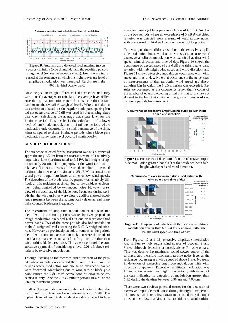
As an example of the effectiveness of the implemented meth-
od for detecting local minima and maxima and calculating
the level of modulation, the results from the automated am-
plitude modulation detection is provided in Figure 9. It shows
the measured noise level for the minute of the 2-minute peri-
od in which the highest level of amplitude modulation was
detected during the 10 days of measurements. Note that the
100 ms sound pressure level is the level in the 800 Hz third
octave band. Overlayed are the local minima and maxima
automatically detected by the algorithm, and the level of
modulation (against the secondary axis), for each maxima
which has been automatically classified as being of blade
pass origin.
Proceedings of Acoustics 2013 – Victor Harbor 17-20 November 2013, Victor Harbor, Australia
Australian Acoustical Society 7
0
5
10
15
0
5
10
15
20
25
30
35
1:00 1:05 1:10 1:15 1:20 1:25 1:30 1:35 1:40 1:45 1:50 1:55 2:00
Mo
du
lati
on
(d
B)
Sou
nd
pre
ssu
re le
vel (
dB
)
Time (minutes:seconds)
Automatic detection and calculation of level of modulation
Measured 100 ms Lp local minima local maxima Level of Modulation
Figure 9. Automatically detected local maxima (green
squares), minima (blue diamonds) and the resulting peak to
trough level (red on the secondary axis), from the 2-minute
period at the residence in which the highest average level of
amplitude modulation was measured. Results are in the
800 Hz third octave band.
Once the peak to trough differences had been calculated, they
were linearly averaged to calculate the average level differ-
ence during that two-minute period in that one-third octave
band or for the overall A-weighted levels. Where modulation
was anticipated based on the regular blade pass spacing but
did not occur a value of 0 dB was used for that missing blade
pass when calculating the average blade pass level for the
2-minute period. This results in the calculation of a lower
level of amplitude modulation in 2-minute periods where
modulation only occurred for a small percentage of the time,
when compared to those 2-minute periods where blade pass
modulation at the same level occurred continuously.
RESULTS AT A RESIDENCE
The residence selected for the assessment was at a distance of
approximately 1.5 km from the nearest turbine of a relatively
large wind farm (turbines rated to 3 MW, hub height of ap-
proximately 80 m). The topography at the wind farm site is
relatively flat. Noise levels at the residence due to the wind
turbines alone was approximately 35 dB(A) at maximum
sound power output, but lower at times of low wind speeds.
The detection of the blade pass frequency was relatively dif-
ficult at this residence at times, due to the ambient environ-
ment being controlled by extraneous noise. However, a re-
view of the accuracy of the blade pass frequency during peri-
ods that the wind turbines were clearly audible showed excel-
lent agreement between the automatically detected and man-
ually counted blade pass frequency.
The assessment of amplitude modulation at the residence
identified 114 2-minute periods where the average peak to
trough modulation exceeded 6 dB in one or more one-third
octave bands. Two of the same periods also had modulation
of the A-weighted level exceeding the 5 dB A-weighted crite-
rion. However as previously stated, a number of the periods
identified to contain excessive modulation were the result of
modulating extraneous noise (often frog noise), rather than
wind turbine blade pass noise. This assessment took the con-
servative approach of considering a level 0.01 dB above cri-
teria to be excessive modulation.
Through listening to the recorded audio for each of the peri-
ods where modulation exceeded the 5 and 6 dB criteria, the
periods where modulation was due to an extraneous source
were discarded. Modulation due to wind turbine blade pass
noise caused the 6 dB third octave band criterion to be ex-
ceeded in only 32 of the 7083 2 minute periods (0.45% or the
total measurement period).
In all of these periods, the amplitude modulation in the rele-
vant one-third octave band was between 6 and 6.5 dB. The
highest level of amplitude modulation due to wind turbine
noise had average blade pass modulation of 6.5 dB. Neither
of the two periods where an exceedance of 5 dB A-weighted
criterion was detected were a result of wind turbine noise,
with one a result of bird and the other a result of frog noise.
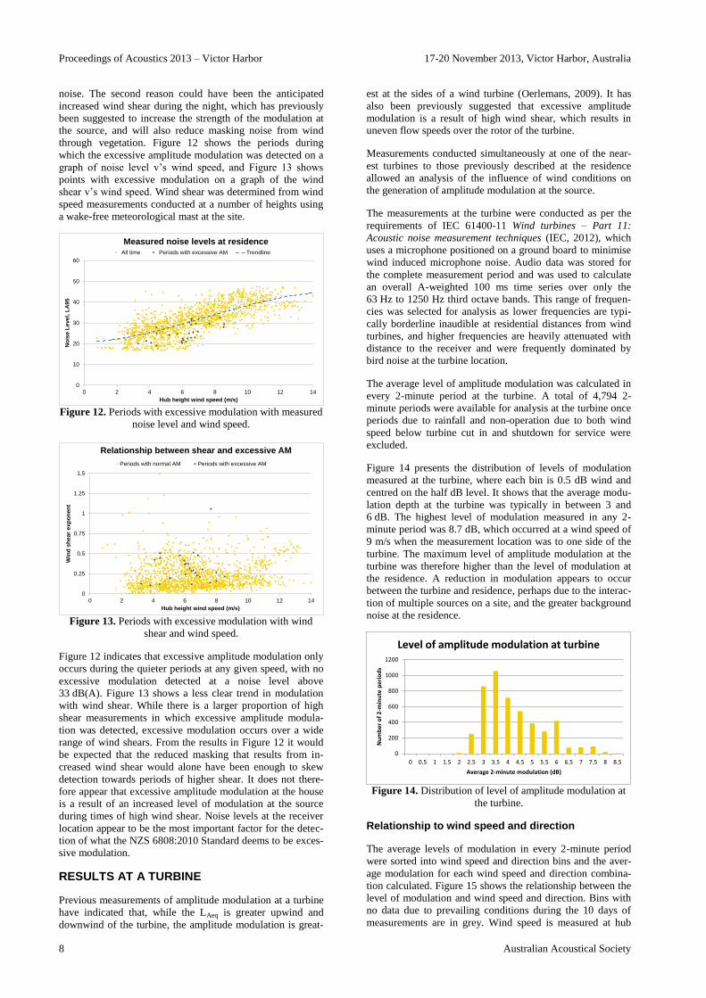
To investigate the conditions resulting in the excessive ampli-
tude modulation due to wind turbine noise, the occurrence of
excessive amplitude modulation was examined against wind
speed, wind direction and time of day. Figure 10 shows the
occurrence of exceedances of the 6 dB one-third octave band
criterion with hub height wind speed and wind direction, and
Figure 11 shows excessive modulation occurrence with wind
speed and time of day. Note that occurrence is the percentage
of measurements in that particular wind speed and direc-
tion/time bin in which the 6 dB criterion was exceeded. Re-
sults are presented as the occurrence rather than a count of
the number of events exceeding criteria so that results are not
skewed to the bins that contained the greatest number of raw
2-minute periods for assessment.
N
NW
W
SW
S
SE
E
NE
N
0 1 2 3 4 5 6 7 8 9 10 11 12 13 14 15 16
Win
d
dir
ecti
on
Wind Speed (m/s)
12-14
10-12
8-10
6-8
4-6
2-4
0-2
Occurrence (%) of excessive amplitude
modulation
Occurrence of excessive amplitude modulation with wind speed and direction
Figure 10. Frequency of detection of one-third octave ampli-
tude modulation greater than 6 dB at the residence, with hub
height wind speed and wind direction.
0:00 - 3:00
3:00 - 6:00
6:00 - 9:00
9:00 - 12:00
12:00 - 15:00
15:00 - 18:00
18:00 - 21:00
21:00 - 00:00
0:00 - 3:00
0 1 2 3 4 5 6 7 8 9 10 11 12 13 14 15 16
Tim
e o
f d
ay
Wind Speed (m/s)
3-4
2-3
1-2
0-1
Occurrence (%) of excessive amplitude
modulation
Occurrence of excessive amplitude modulation with wind speed and time of day
Figure 11. Frequency of detection of third octave amplitude
modulation greater than 6 dB at the residence, with hub
height wind speed and time of day.
From Figures 10 and 11, excessive amplitude modulation
was limited to hub height wind speeds of between 3 and
9 m/s, although detection at speeds above 7 m/s was rare.
This was despite the maximum sound power output of the
turbines, and therefore maximum turbine noise level at the
residence, occurring at a wind speed of above 9 m/s. No trend
in detection of excessive amplitude modulation with wind
direction is apparent. Excessive amplitude modulation was
limited to the evening and night time periods, with review of
the data indicating no detection of modulation greater than
6 dB during the daytime between 6:30 am and 7:00 pm.
There were two obvious potential causes for the detection of
excessive amplitude modulation during the night time period.
The first is that there is less extraneous noise during the night
time, and so less masking noise to hide the wind turbine
Proceedings of Acoustics 2013 – Victor Harbor 17-20 November 2013, Victor Harbor, Australia
8 Australian Acoustical Society
noise. The second reason could have been the anticipated
increased wind shear during the night, which has previously
been suggested to increase the strength of the modulation at
the source, and will also reduce masking noise from wind
through vegetation. Figure 12 shows the periods during
which the excessive amplitude modulation was detected on a
graph of noise level v’s wind speed, and Figure 13 shows
points with excessive modulation on a graph of the wind
shear v’s wind speed. Wind shear was determined from wind
speed measurements conducted at a number of heights using
a wake-free meteorological mast at the site.
0
10
20
30
40
50
60
0 2 4 6 8 10 12 14
No
ise L
evel, L
A95
Hub height wind speed (m/s)
Measured noise levels at residence All time Periods with excessive AM Trendline
Figure 12. Periods with excessive modulation with measured
noise level and wind speed.
0
0.25
0.5
0.75
1
1.25
1.5
0 2 4 6 8 10 12 14
Win
d s
hear
exp
on
en
t
Hub height wind speed (m/s)
Relationship between shear and excessive AM
Periods with normal AM Periods with excessive AM
Figure 13. Periods with excessive modulation with wind
shear and wind speed.
Figure 12 indicates that excessive amplitude modulation only
occurs during the quieter periods at any given speed, with no
excessive modulation detected at a noise level above
33 dB(A). Figure 13 shows a less clear trend in modulation
with wind shear. While there is a larger proportion of high
shear measurements in which excessive amplitude modula-
tion was detected, excessive modulation occurs over a wide
range of wind shears. From the results in Figure 12 it would
be expected that the reduced masking that results from in-
creased wind shear would alone have been enough to skew
detection towards periods of higher shear. It does not there-
fore appear that excessive amplitude modulation at the house
is a result of an increased level of modulation at the source
during times of high wind shear. Noise levels at the receiver
location appear to be the most important factor for the detec-
tion of what the NZS 6808:2010 Standard deems to be exces-
sive modulation.
RESULTS AT A TURBINE
Previous measurements of amplitude modulation at a turbine
have indicated that, while the LAeq is greater upwind and
downwind of the turbine, the amplitude modulation is great-
est at the sides of a wind turbine (Oerlemans, 2009). It has
also been previously suggested that excessive amplitude
modulation is a result of high wind shear, which results in
uneven flow speeds over the rotor of the turbine.
Measurements conducted simultaneously at one of the near-
est turbines to those previously described at the residence
allowed an analysis of the influence of wind conditions on
the generation of amplitude modulation at the source.
The measurements at the turbine were conducted as per the
requirements of IEC 61400-11 Wind turbines – Part 11:
Acoustic noise measurement techniques (IEC, 2012), which
uses a microphone positioned on a ground board to minimise
wind induced microphone noise. Audio data was stored for
the complete measurement period and was used to calculate
an overall A-weighted 100 ms time series over only the
63 Hz to 1250 Hz third octave bands. This range of frequen-
cies was selected for analysis as lower frequencies are typi-
cally borderline inaudible at residential distances from wind
turbines, and higher frequencies are heavily attenuated with
distance to the receiver and were frequently dominated by
bird noise at the turbine location.
The average level of amplitude modulation was calculated in
every 2-minute period at the turbine. A total of 4,794 2-
minute periods were available for analysis at the turbine once
periods due to rainfall and non-operation due to both wind
speed below turbine cut in and shutdown for service were
excluded.
Figure 14 presents the distribution of levels of modulation
measured at the turbine, where each bin is 0.5 dB wind and
centred on the half dB level. It shows that the average modu-
lation depth at the turbine was typically in between 3 and
6 dB. The highest level of modulation measured in any 2-
minute period was 8.7 dB, which occurred at a wind speed of
9 m/s when the measurement location was to one side of the
turbine. The maximum level of amplitude modulation at the
turbine was therefore higher than the level of modulation at
the residence. A reduction in modulation appears to occur
between the turbine and residence, perhaps due to the interac-
tion of multiple sources on a site, and the greater background
noise at the residence.
0
200
400
600
800
1000
1200
0 0.5 1 1.5 2 2.5 3 3.5 4 4.5 5 5.5 6 6.5 7 7.5 8 8.5
Nu
mb
er
of
2-m
inu
te p
eri
od
s
Average 2-minute modulation (dB)
Level of amplitude modulation at turbine
Figure 14. Distribution of level of amplitude modulation at
the turbine.
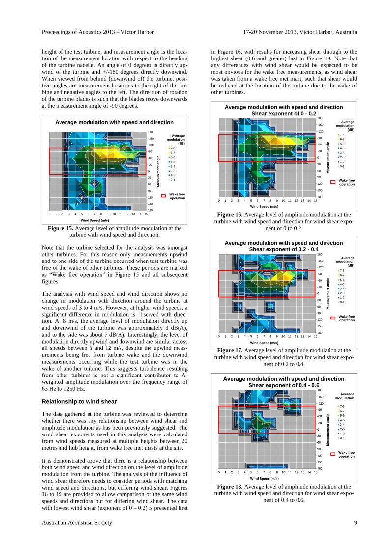
Relationship to wind speed and direction
The average levels of modulation in every 2-minute period
were sorted into wind speed and direction bins and the aver-
age modulation for each wind speed and direction combina-
tion calculated. Figure 15 shows the relationship between the
level of modulation and wind speed and direction. Bins with
no data due to prevailing conditions during the 10 days of
measurements are in grey. Wind speed is measured at hub
Proceedings of Acoustics 2013 – Victor Harbor 17-20 November 2013, Victor Harbor, Australia
Australian Acoustical Society 9
height of the test turbine, and measurement angle is the loca-
tion of the measurement location with respect to the heading
of the turbine nacelle. An angle of 0 degrees is directly up-
wind of the turbine and +/-180 degrees directly downwind.
When viewed from behind (downwind of) the turbine, posi-
tive angles are measurement locations to the right of the tur-
bine and negative angles to the left. The direction of rotation
of the turbine blades is such that the blades move downwards
at the measurement angle of -90 degrees.
180
150
120
90
60
30
0
-30
-60
-90
-120
-150
180
0 1 2 3 4 5 6 7 8 9 10 11 12 13 14 15
Me
as
ure
me
nt
an
gle
Wind Speed (m/s)
7-8
6-7
5-6
4-5
3-4
2-3
1-2
0-1
Average modulation
(dB)
Average modulation with speed and direction
Wake free operation
Figure 15. Average level of amplitude modulation at the
turbine with wind speed and direction.
Note that the turbine selected for the analysis was amongst
other turbines. For this reason only measurements upwind
and to one side of the turbine occurred when test turbine was
free of the wake of other turbines. These periods are marked
as “Wake free operation” in Figure 15 and all subsequent
figures.
The analysis with wind speed and wind direction shows no
change in modulation with direction around the turbine at
wind speeds of 3 to 4 m/s. However, at higher wind speeds, a
significant difference in modulation is observed with direc-
tion. At 8 m/s, the average level of modulation directly up
and downwind of the turbine was approximately 3 dB(A),
and to the side was about 7 dB(A). Interestingly, the level of
modulation directly upwind and downwind are similar across
all speeds between 3 and 12 m/s, despite the upwind meas-
urements being free from turbine wake and the downwind
measurements occurring while the test turbine was in the
wake of another turbine. This suggests turbulence resulting
from other turbines is not a significant contributor to A-
weighted amplitude modulation over the frequency range of
63 Hz to 1250 Hz.
Relationship to wind shear
The data gathered at the turbine was reviewed to determine
whether there was any relationship between wind shear and
amplitude modulation as has been previously suggested. The
wind shear exponents used in this analysis were calculated
from wind speeds measured at multiple heights between 20
metres and hub height, from wake free met masts at the site.
It is demonstrated above that there is a relationship between
both wind speed and wind direction on the level of amplitude
modulation from the turbine. The analysis of the influence of
wind shear therefore needs to consider periods with matching
wind speed and directions, but differing wind shear. Figures
16 to 19 are provided to allow comparison of the same wind
speeds and directions but for differing wind shear. The data
with lowest wind shear (exponent of 0 – 0.2) is presented first
in Figure 16, with results for increasing shear through to the
highest shear (0.6 and greater) last in Figure 19. Note that
any differences with wind shear would be expected to be
most obvious for the wake free measurements, as wind shear
was taken from a wake free met mast, such that shear would
be reduced at the location of the turbine due to the wake of
other turbines.
180
150
120
90
60
30
0
-30
-60
-90
-120
-150
180
0 1 2 3 4 5 6 7 8 9 10 11 12 13 14 15
Me
as
ure
me
nt
an
gle
Wind Speed (m/s)
7-8
6-7
5-6
4-5
3-4
2-3
1-2
0-1
Average modulation
(dB)
Average modulation with speed and directionShear exponent of 0 - 0.2
Wake free operation
Figure 16. Average level of amplitude modulation at the
turbine with wind speed and direction for wind shear expo-
nent of 0 to 0.2.
180
150
120
90
60
30
0
-30
-60
-90
-120
-150
180
0 1 2 3 4 5 6 7 8 9 10 11 12 13 14 15
Me
as
ure
me
nt
an
gle
Wind Speed (m/s)
7-8
6-7
5-6
4-5
3-4
2-3
1-2
0-1
Average modulation
(dB)
Average modulation with speed and directionShear exponent of 0.2 - 0.4
Wake free operation
Figure 17. Average level of amplitude modulation at the
turbine with wind speed and direction for wind shear expo-
nent of 0.2 to 0.4.
Figure 18. Average level of amplitude modulation at the
turbine with wind speed and direction for wind shear expo-
nent of 0.4 to 0.6.
Proceedings of Acoustics 2013 – Victor Harbor 17-20 November 2013, Victor Harbor, Australia
10 Australian Acoustical Society
180
150
120
90
60
30
0
-30
-60
-90
-120
-150
180
0 1 2 3 4 5 6 7 8 9 10 11 12 13 14 15M
ea
su
rem
en
t a
ng
le
Wind Speed (m/s)
7-8
6-7
5-6
4-5
3-4
2-3
1-2
0-1
Average modulation
(dB)
Average modulation with speed and directionShear exponent of 0.6 and above
Wake free operation
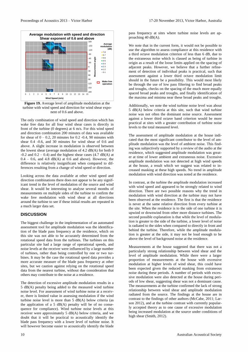
Figure 19. Average level of amplitude modulation at the
turbine with wind speed and direction for wind shear expo-
nent of 0.6 and above.
The only combination of wind speed and direction which has
wake free data for all four wind shear cases is directly in
front of the turbine (0 degrees) at 6 m/s. For this wind speed
and direction combination 200 minutes of data was available
for shear of 0 – 0.2, 20 minutes for 0.2 -0.4, 90 minutes with
shear 0.4 -0.6, and 30 minutes for wind shear of 0.6 and
above. A slight increase in modulation is observed between
the lowest shear (average modulation of 4.2 dB(A) for both 0
-0.2 and 0.2 – 0.4) and the highest shear cases (4.7 dB(A) at
0.4 – 0.6, and 4.8 dB(A) at 0.6 and above). However, the
difference is relatively insignificant when compared to dif-
ferences resulting from a change of wind speed or direction.
Looking across the data available at other wind speed and
direction combinations there does not appear to be any signif-
icant trend in the level of modulation of the source and wind
shear. It would be interesting to analyse several months of
measurements on multiple sides of the turbine to confirm the
wake free modulation with wind shear at all directions
around the turbine to see if these initial results are repeated in
a much larger data set.
DISCUSSION
The biggest challenge in the implementation of an automated
assessment tool for amplitude modulation was the identifica-
tion of the blade pass frequency at the residence, which on
this site was not able to be accurately determined from the
rotational speed data from the turbines. The turbines on this
particular site had a large range of operational speeds, and
noise levels at the receiver were influenced by a large number
of turbines, rather than being controlled by one or two tur-
bines. It may be the case the rotational speed data provides a
more accurate measure of the blade pass frequency at other
sites, but we caution against relying on the rotational speed
data from the nearest turbine, without due consideration that
others may contribute to the noise at a residence.
The detection of excessive amplitude modulation results in a
5 dB(A) penalty being added to the measured wind turbine
noise level. For assessment of wind turbine noise at a receiv-
er, there is limited value in assessing modulation if the wind
turbine noise level is more than 5 dB(A) below criteria (as
the application of a 5 dB(A) penalty will be of no conse-
quence for compliance). Wind turbine noise levels at this
receiver were approximately 5 dB(A) below criteria, and we
doubt that it will be practical to acoustically identify the
blade pass frequency with a lower level of turbine noise. It
will however become easier to acoustically identify the blade
pass frequency at sites where turbine noise levels are ap-
proaching 40 dB(A).
We note that in the current form, it would not be possible to
use the algorithm to assess compliance at this residence with
a third octave modulation criterion of less than 6 dB, due to
the extraneous noise which is classed as being of turbine in
origin as a result of the loose limits applied on the spacing of
adjacent peaks. However, we believe that a further refine-
ment of detection of individual peaks is practical, such that
assessment against a lower third octave modulation limit
should in the future be a possibility. This would most likely
be through the use of low pass filtering to find broad peaks
and troughs, checks on the spacing of the much more equally
spaced broad peaks and troughs, and finally identification of
the maxima and minima near these broad peaks and troughs.
Additionally, we note the wind turbine noise level was about
5 dB(A) below criteria at this site, such that wind turbine
noise was not often the dominant noise source. Assessment
against a lower third octave band criterion would be more
practical at sites with a greater contribution of turbine noise
levels to the total measured level.
The assessment of amplitude modulation at the house indi-
cated that the most significant contributor to the level of am-
plitude modulation was the level of ambient noise. This find-
ing was subjectively supported by a review of the audio at the
residence, which suggested amplitude modulation was great-
er at time of lower ambient and extraneous noise. Excessive
amplitude modulation was not detected at high wind speeds
at the house, a result which we suggest was related to in-
creased masking at these high speeds. No trend in amplitude
modulation with wind direction was noted at the residence.
In contrast, at the turbine the amplitude modulation increased
with wind speed and appeared to be strongly related to wind
direction. There are two possible reasons why the trend in
modulation with wind direction at the turbine may not have
been observed at the residence. The first is that the residence
is never at the same relative direction from every turbine at
the site. When the residence is to the side of one turbine it is
upwind or downwind from other more distance turbines. The
second possible explanation is that while the level of modula-
tion is greater to the side of the turbine, a lower level of noise
is radiated to the sides when compared to directly in front and
behind the turbine. Therefore, while the amplitude modula-
tion is greater at the side, it may not be loud enough to be
above the level of background noise at the residence.
Measurements at the house suggested that there was not a
particularly strong relationship between wind shear and the
level of amplitude modulation. While there were a larger
proportion of measurements at the house with excessive
modulation at higher levels of wind shear, this could have
been expected given the reduced masking from extraneous
noise during these periods. A number of periods with exces-
sive modulation were also detected at the house during peri-
ods of low shear, suggesting shear was not a dominant cause.
The measurements at the turbine confirmed the lack of strong
relationship between wind shear and amplitude modulation
radiated from the source. The findings at the house are in
contrast to the findings of other authors (McCabe, 2011; Lar-
son 2012), and at the turbine contrast with currently popular-
ly accepted theory as to one cause of excessive modulation
being increased modulation at the source under conditions of
high shear (Smith, 2012).
Proceedings of Acoustics 2013 – Victor Harbor 17-20 November 2013, Victor Harbor, Australia
Australian Acoustical Society 11
It would be interesting to review modulation at the house and
turbine for a period of several months to see if this initial
finding is upheld. However, the explanation for the difference
at the house may be as suggested by McCabe, that the in-
crease in modulation at distance during periods of higher
shear in his measurements was more a result of reduced
masking at the receiver than an increase in modulation at the
source. This explanation is supported by Søndergaard (2012),
who found similar levels of modulation under unstable condi-
tions during daytime as under stable conditions at night.
The lack of a significant increase in modulation at the source
may have been the result of insufficient wind shear during the
measurement period to cause stall, although there were sev-
eral periods with shear exponent of greater than 1. It may also
be that modern turbines are less susceptible to excessive
modulation due to periods of high shear than the previous
generation of stall regulated turbines that were common when
excessive amplitude modulation was first reported.
The lack of a relationship between stall and modulation at the
turbine might indicate that modulation judged to be ‘exces-
sive’ at this residence under the 6 dB third octave test includ-
ed in NZS 6808:2010 was actually just ‘normal’ modulation.
The audio captured at the residence during these periods of
‘excessive’ modulation did not subjectively sound signifi-
cantly different in character.
One final issue that needs to be addressed in the assessment
of amplitude modulation at residence is the development of
dose response relationships, to provide sound justification of
the criterion levels currently adopted by the various standards
and guidelines used globally. In recognition of the lack of
information around the subjective response of listeners to
amplitude modulation, one part of the research currently
being funded by RenewableUK focuses on the subjective
response of listeners to amplitude modulation. From publical-
ly available information it appears that work is focusing on
an RMS criterion level (Cand, 2012), which may not be di-
rectly applicable to the peak to trough assessment criteria like
that currently suggested by NZS 6808:2010.
CONCLUSION
This paper has provided a summary of the development of an
algorithm for the assessment of amplitude modulation against
the requirements of Appendix B of NZS 6808:2010. Addi-
tionally, the findings of an assessment at a residence have
been provided, along with the results of an analysis of modu-
lation at an adjacent turbine.
On the balance of the available data at the residence it would
appear that the ambient noise level at the residence is a more
important factor in the detection of excessive amplitude than
the influence of wind shear. Periods judged to be ‘excessive’
modulation using the 6 dB third octave test in NZS
6808:2010 occurred at the residence under periods of both
low and high wind shear. Measurements at the turbine sug-
gested a negligible influence from wind shear on the genera-
tion of amplitude modulation at the source. Review of modu-
lation at the source also indicated no significant increase in
modulation from turbulence, which occurs when the turbine
is operating in the wake of another.
The lack of increase in modulation at the source during peri-
ods of wind shear suggests the modulation at the site might
be best described as ‘normal’ wind turbine noise modulation
with a ‘swish’ character, rather than ‘excessive’ modulation
with a ‘thumping’ nature. This finding was supported by a
review of audio at both the residence and turbine, which did
not find any obvious change in the character of the sound.
Further work is required to determine whether the 6 dB crite-
rion level for modulation depth of third octave noise provides
a suitable test of ‘excessive’ modulation, and to determine a
dose response against which the level of increased annoyance
can be determined. This 6 dB criterion was regularly exceed-
ed close to the turbine when measuring at high wind speeds
to the side of the turbine. The findings at this residence sug-
gest this criterion may also be occasionally exceeded at resi-
dential distances during periods of ‘normal’ modulation.
REFERENCES
Bowdler D, Papers and publications, viewed 12 August 2013
http://www.dickbowdler.co.uk/content/publications/
Cand MM, Bullmore AJ, Smith M, Von-Hunerbein S & Da-
vis R, ‘Wind turbine amplitude modulation: research to
improve understanding as to its cause & effect’, Proceed-
ings of Acoustics 2012, Nantes, 23-27 April 2012
Bass J, Bowdler D, McCaffery M and Grimes G, ‘Fundamen-
tal Research in Amplitude Modulation – a Project by Re-
newableUK’, Procedings of Wind Turbine Noise 2011,
Rome, 12 – 14 April 2011.
Flow Solutions Ltd, Hoare Lea & Partners Acoustics: Re-
newable Energy Systems Ltd. “Wind Turbine Measure-
ments for Noise Source Identification: ETSU
W/13/00391/REP, 1999
IEC 2012, Wind turbines – Part 11: Acoustic noise measure-
ment techniques, IEC 61400-11 Edition 3.0, International
Electrotechnical Commission, Geneva.
Larsson C & Öhlund O, ‘Variations of sound from wind tur-
bines during different weather Conditions’, Proceedings
of Internoise 2012, New York, 19-22 August 2012.
Lee S, Kim K, Lee S, Kim H & Lee S, ‘An estimation meth-
od of the amplitude modulation in wind turbine noise for
community response assessment’, Procedings of Wind
Turbine Noise 2009, Denmark, 17 – 19 June 2009.
Lee S, Kim K, Choi W & Lee S, "Annoyance caused by am-
plitude modulation of wind turbine noise," Noise Control
Engineering Journal, Vol 59, 38-46, 2011.
Moorhouse A, Hayes M, von Hünerbein S, Piper B & Adams
M, ‘Research into Aerodynamic Modulation of Wind
Turbine Noise: Final report’, University of Salford, July
2007.
McCabe JN ‘Detection and Quantification of Amplitude
Modulation in Wind Turbine Noise’, Proceedings of
Wind Turbine Noise 2011, Rome, 12 – 14 April 2011.
Oerlemans S, Sijtsma P & Méndez López B, ‘Location and
quantification of noise sources on a wind turbine’, Jour-
nal of Sound and Vibration, Vol 299, 869-883, 2007.
Oerlemans S & Schepers G, ‘Prediction of wind turbine noise
directivity and swish’, Proceedings of Wind Turbine
Noise 2009, Denmark, 17 – 19 June 2009.
SA EPA 2009, Wind farms environmental noise guidelines,
Environment Protection Authority, Adelaide.
Smith M, Bullmore AJ, Cand MM & Davis R, ‘Mechanisms
of amplitude modulation in wind turbine noise’, Proceed-
ings of Acoustics 2012, Nantes, 23-27 April 2012
Søndergaard LS, ‘Noise from wind turbines under non-
standard conditions’, Proceedings of Internoise 2012,
New York, 19-22 August 2012.
Standards Australia, 2010, Acoustics – Measurement, predic-
tion and assessment of noise from wind turbine genera-
tors, AS 4959-2010, Standards Australia, Sydney.
Standards New Zealand, 2010, Acoustics – Wind farm noise,
NZS 6808:2010, Standards New Zealand, Wellington.