Embed Size (px)
Citation preview
Automated Debugging Framework for
High-level Synthesis
by
Li Liu
A thesis submitted in conformity with the requirementsfor the degree of Master of Applied Science
Graduate Department of Electrical and Computer EngineeringUniversity of Toronto
Copyright c© 2013 by Li Liu
Abstract
Automated Debugging Framework for
High-level Synthesis
Li Liu
Master of Applied Science
Graduate Department of Electrical and Computer Engineering
University of Toronto
2013
High-level synthesis (HLS) is an automatic compilation technique that translates a soft-
ware program to a hardware circuit [10]. This process is intended to make hardware
design easier. HLS techniques have been studied for more than 20 years and a number
of HLS tools have been developed in both industry and academia. However, verifying
correctness of HLS tools can sometimes be difficult due to a lack of benchmarks.
This thesis proposes an automated test case generation technique for verifying/debugging
HLS tools. The work presented in this thesis builds a framework that automatically gen-
erates random programs with user-specified features/characteristics. These programs are
used to verify the correctness of HLS tools by comparing the output of hardware gener-
ated by HLS to the original software. Thus, users can have a large number of benchmarks
to test their HLS algorithms without having to manually develop test programs. The
framework also provides additional ways of analyzing the performance of HLS tools.
Rather than being a replacement to the existing verification tools, this debugging
framework should serve as a useful complement to other existing test suites. Together,
they can provide a more comprehensive verification/debugging and analysis for HLS
tools.
ii

Acknowledgements
First, I would like to thank my parents for raising me and giving me the chance to study
abroad. They have always given me support spiritually and financially.
I would like to thank Professor Stephen Brown for financially supporting me and
giving me the opportunity to work in this research group and to be a part of such an
intriguing research project.
I would like to thank Professor Jason Anderson for all the daily summer meetings,
weekly status meetings, and for the many insightful ideas and suggestions. Both of you
and Professor Brown have been amazing mentors.
I would like to thank Professor Nicola Nicolici from McMaster University. You are
the person who brought me into this field. I will always remember that you told me,
“don’t behave like currents who always take the low pass. Instead, take the high pass,
you will gain more eventually.”
I would also like to thank Andrew Canis for the numerous discussions and help and
Jongsok Choi for helping me with my grammar checking and thesis writing.
In addition, I would like to thank my girlfriend, Sue, for all times you knocked on my
head and asked me to sleep early even though I rarely do.
At last, I would like to thank all my friends for all the good times we had together.
iii
Contents
1 Introduction 1
1.1 Motivation . . . . . . . . . . . . . . . . . . . . . . . . . . . . . . . . . . . 1
1.2 Contributions . . . . . . . . . . . . . . . . . . . . . . . . . . . . . . . . . 3
1.3 Thesis Organization . . . . . . . . . . . . . . . . . . . . . . . . . . . . . . 3
2 Background 4
2.1 High-Level Synthesis . . . . . . . . . . . . . . . . . . . . . . . . . . . . . 4
2.2 LegUp . . . . . . . . . . . . . . . . . . . . . . . . . . . . . . . . . . . . . 5
2.3 LLVM Intermediate Representation . . . . . . . . . . . . . . . . . . . . . 5
2.4 Control Flow Graph and Data Flow Graph . . . . . . . . . . . . . . . . . 6
2.4.1 Control flow graph (CFG) . . . . . . . . . . . . . . . . . . . . . . 6
2.4.2 Data flow graph (DFG) . . . . . . . . . . . . . . . . . . . . . . . 6
2.5 Resource sharing and pattern matching in HLS . . . . . . . . . . . . . . 7
2.6 Verification techniques for HLS . . . . . . . . . . . . . . . . . . . . . . . 8
2.6.1 Formal Verification . . . . . . . . . . . . . . . . . . . . . . . . . . 8
2.6.2 Assertion-based Verification . . . . . . . . . . . . . . . . . . . . . 10
2.6.3 Manually developed test suites . . . . . . . . . . . . . . . . . . . . 11
3 Implementation 13
3.1 Overall debugging flow . . . . . . . . . . . . . . . . . . . . . . . . . . . . 13
3.2 Test case generation . . . . . . . . . . . . . . . . . . . . . . . . . . . . . 14
iv
3.2.1 Parameters used in the generator . . . . . . . . . . . . . . . . . . 14
3.2.1.1 Size control . . . . . . . . . . . . . . . . . . . . . . . . . 17
3.2.1.2 Structure control . . . . . . . . . . . . . . . . . . . . . . 18
3.2.2 Summary of parameters . . . . . . . . . . . . . . . . . . . . . . . 19
3.2.3 Graph generation . . . . . . . . . . . . . . . . . . . . . . . . . . . 20
3.2.3.1 Graph Structure . . . . . . . . . . . . . . . . . . . . . . 20
3.2.3.2 CFG generation . . . . . . . . . . . . . . . . . . . . . . . 22
3.2.3.3 CFG loop generation . . . . . . . . . . . . . . . . . . . . 25
3.2.3.4 Multiple hierarchies of CFGs . . . . . . . . . . . . . . . 27
3.2.3.5 DFG generation . . . . . . . . . . . . . . . . . . . . . . 28
3.2.3.6 Patterns in DFG . . . . . . . . . . . . . . . . . . . . . . 33
3.2.4 LLVM IR generation . . . . . . . . . . . . . . . . . . . . . . . . . 34
3.2.5 Generate main wrapper function . . . . . . . . . . . . . . . . . . 39
3.3 HW/SW results verification and Analysis . . . . . . . . . . . . . . . . . . 40
3.4 Summary . . . . . . . . . . . . . . . . . . . . . . . . . . . . . . . . . . . 40
4 Experiments 41
4.1 Effect of depth factor . . . . . . . . . . . . . . . . . . . . . . . . . . . . . 41
4.2 Analysis of pattern matching . . . . . . . . . . . . . . . . . . . . . . . . . 42
4.3 An alternative binding algorithm . . . . . . . . . . . . . . . . . . . . . . 44
4.4 Runtime analysis for LegUp’s pattern matching algorithm . . . . . . . . 47
4.5 Comparison with CHStone . . . . . . . . . . . . . . . . . . . . . . . . . . 47
4.5.1 Diversity: CHStone vs. Auto-generated test cases . . . . . . . . . 49
4.5.1.1 Diversity of CHStone test suite . . . . . . . . . . . . . . 49
4.5.1.2 Diversity of auto-generated test cases . . . . . . . . . . . 50
4.5.2 Size: CHStone vs. Auto-generated test cases . . . . . . . . . . . . 51
4.5.2.1 Size of CHStone test suite . . . . . . . . . . . . . . . . . 51
4.5.2.2 Size of auto-generated test cases . . . . . . . . . . . . . 53
v
4.5.3 Synthesizability: CHStone vs. Auto-generated test cases . . . . . 54
4.5.3.1 Synthesizability of CHStone test suite . . . . . . . . . . 54
4.5.3.2 Synthesizability of auto-generated test cases . . . . . . . 54
4.5.4 Usability: CHStone vs. Auto-generated test cases . . . . . . . . . 55
4.5.4.1 Usability of CHStone test suite . . . . . . . . . . . . . . 55
4.5.4.2 Usability of auto-generated test cases . . . . . . . . . . . 55
4.5.5 Code coverage comparison . . . . . . . . . . . . . . . . . . . . . . 56
4.5.5.1 CHStone code coverage in LegUp . . . . . . . . . . . . . 56
4.5.5.2 Auto generated test programs code coverage in LegUp . 57
4.6 Bugs detected in LegUp 2.0 release . . . . . . . . . . . . . . . . . . . . . 59
4.6.1 Problem with shift instructions . . . . . . . . . . . . . . . . . . . 59
4.6.2 A LegUp produced Verilog file hangs at Quartus II compilation . 62
4.7 Detecting injected bugs in LegUp . . . . . . . . . . . . . . . . . . . . . . 62
4.7.1 Disabling Live Variable Analysis . . . . . . . . . . . . . . . . . . . 62
5 Conclusion 64
5.1 Summary . . . . . . . . . . . . . . . . . . . . . . . . . . . . . . . . . . . 64
5.2 Future work . . . . . . . . . . . . . . . . . . . . . . . . . . . . . . . . . . 65
5.2.1 Input vector range analysis for test programs . . . . . . . . . . . . 65
5.2.2 Back tracing the error points . . . . . . . . . . . . . . . . . . . . 65
5.2.3 Customizable pattern injection . . . . . . . . . . . . . . . . . . . 66
A Add new operation type to the framework 67
B Experimental results for replicating patterns in a single basic block 70
C Experimental results for replicating basic blocks 74
D Experimental results for pattern matching runtime 89
vi

E Experimental results for size factor 95
F Experimental results for depth factor effects 101
Bibliography 107
vii
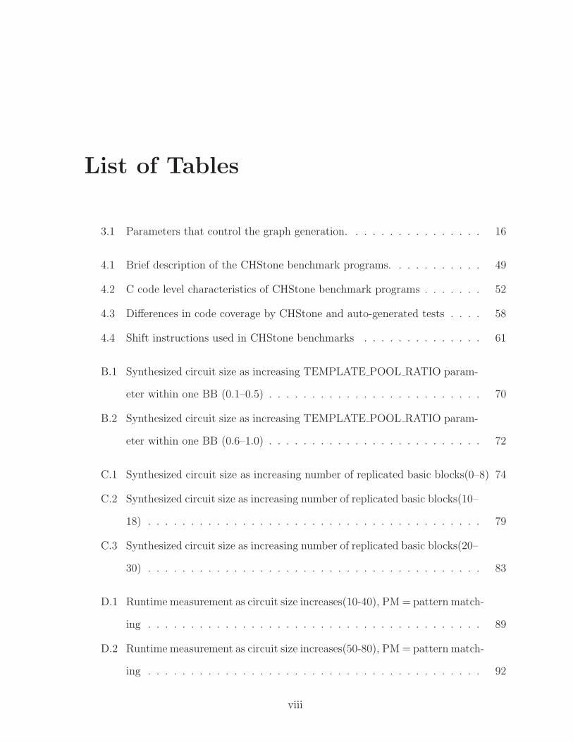
List of Tables
3.1 Parameters that control the graph generation. . . . . . . . . . . . . . . . 16
4.1 Brief description of the CHStone benchmark programs. . . . . . . . . . . 49
4.2 C code level characteristics of CHStone benchmark programs . . . . . . . 52
4.3 Differences in code coverage by CHStone and auto-generated tests . . . . 58
4.4 Shift instructions used in CHStone benchmarks . . . . . . . . . . . . . . 61
B.1 Synthesized circuit size as increasing TEMPLATE POOL RATIO param-
eter within one BB (0.1–0.5) . . . . . . . . . . . . . . . . . . . . . . . . . 70
B.2 Synthesized circuit size as increasing TEMPLATE POOL RATIO param-
eter within one BB (0.6–1.0) . . . . . . . . . . . . . . . . . . . . . . . . . 72
C.1 Synthesized circuit size as increasing number of replicated basic blocks(0–8) 74
C.2 Synthesized circuit size as increasing number of replicated basic blocks(10–
18) . . . . . . . . . . . . . . . . . . . . . . . . . . . . . . . . . . . . . . . 79
C.3 Synthesized circuit size as increasing number of replicated basic blocks(20–
30) . . . . . . . . . . . . . . . . . . . . . . . . . . . . . . . . . . . . . . . 83
D.1 Runtime measurement as circuit size increases(10-40), PM= pattern match-
ing . . . . . . . . . . . . . . . . . . . . . . . . . . . . . . . . . . . . . . . 89
D.2 Runtime measurement as circuit size increases(50-80), PM= pattern match-
ing . . . . . . . . . . . . . . . . . . . . . . . . . . . . . . . . . . . . . . . 92
viii
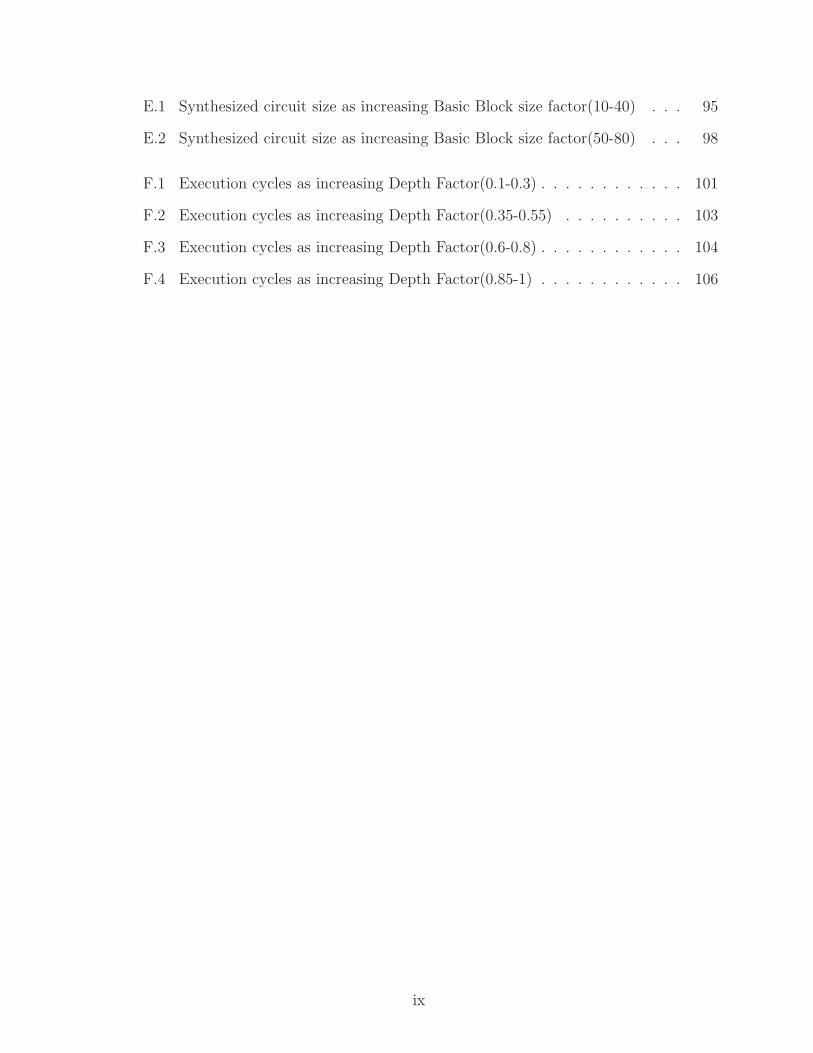
E.1 Synthesized circuit size as increasing Basic Block size factor(10-40) . . . 95
E.2 Synthesized circuit size as increasing Basic Block size factor(50-80) . . . 98
F.1 Execution cycles as increasing Depth Factor(0.1-0.3) . . . . . . . . . . . . 101
F.2 Execution cycles as increasing Depth Factor(0.35-0.55) . . . . . . . . . . 103
F.3 Execution cycles as increasing Depth Factor(0.6-0.8) . . . . . . . . . . . . 104
F.4 Execution cycles as increasing Depth Factor(0.85-1) . . . . . . . . . . . . 106
ix
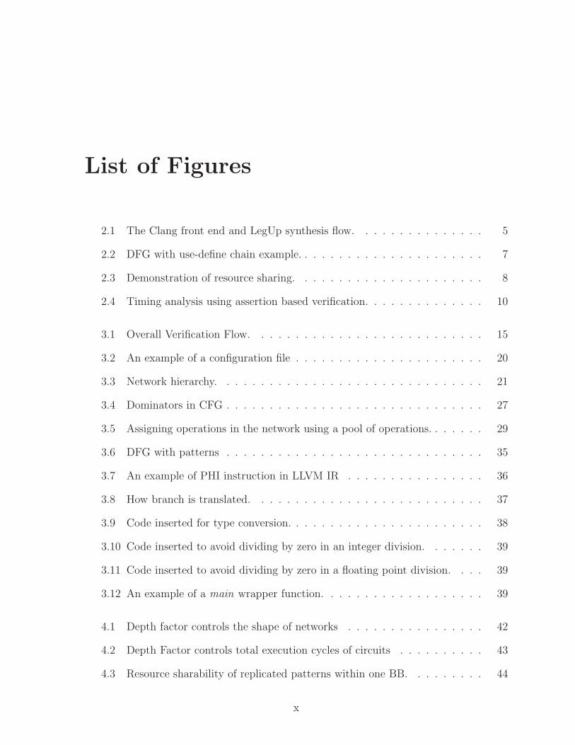
List of Figures
2.1 The Clang front end and LegUp synthesis flow. . . . . . . . . . . . . . . 5
2.2 DFG with use-define chain example. . . . . . . . . . . . . . . . . . . . . . 7
2.3 Demonstration of resource sharing. . . . . . . . . . . . . . . . . . . . . . 8
2.4 Timing analysis using assertion based verification. . . . . . . . . . . . . . 10
3.1 Overall Verification Flow. . . . . . . . . . . . . . . . . . . . . . . . . . . 15
3.2 An example of a configuration file . . . . . . . . . . . . . . . . . . . . . . 20
3.3 Network hierarchy. . . . . . . . . . . . . . . . . . . . . . . . . . . . . . . 21
3.4 Dominators in CFG . . . . . . . . . . . . . . . . . . . . . . . . . . . . . . 27
3.5 Assigning operations in the network using a pool of operations. . . . . . . 29
3.6 DFG with patterns . . . . . . . . . . . . . . . . . . . . . . . . . . . . . . 35
3.7 An example of PHI instruction in LLVM IR . . . . . . . . . . . . . . . . 36
3.8 How branch is translated. . . . . . . . . . . . . . . . . . . . . . . . . . . 37
3.9 Code inserted for type conversion. . . . . . . . . . . . . . . . . . . . . . . 38
3.10 Code inserted to avoid dividing by zero in an integer division. . . . . . . 39
3.11 Code inserted to avoid dividing by zero in a floating point division. . . . 39
3.12 An example of a main wrapper function. . . . . . . . . . . . . . . . . . . 39
4.1 Depth factor controls the shape of networks . . . . . . . . . . . . . . . . 42
4.2 Depth Factor controls total execution cycles of circuits . . . . . . . . . . 43
4.3 Resource sharability of replicated patterns within one BB. . . . . . . . . 44
x
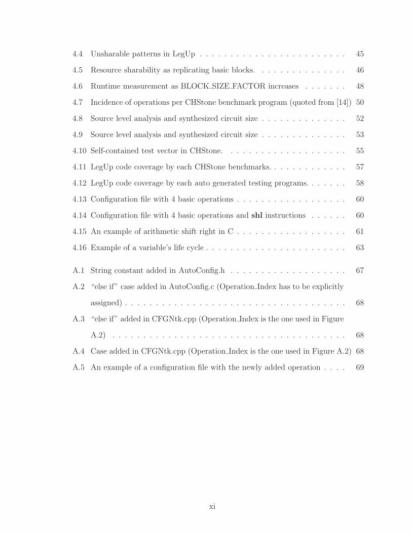
4.4 Unsharable patterns in LegUp . . . . . . . . . . . . . . . . . . . . . . . . 45
4.5 Resource sharability as replicating basic blocks. . . . . . . . . . . . . . . 46
4.6 Runtime measurement as BLOCK SIZE FACTOR increases . . . . . . . 48
4.7 Incidence of operations per CHStone benchmark program (quoted from [14]) 50
4.8 Source level analysis and synthesized circuit size . . . . . . . . . . . . . . 52
4.9 Source level analysis and synthesized circuit size . . . . . . . . . . . . . . 53
4.10 Self-contained test vector in CHStone. . . . . . . . . . . . . . . . . . . . 55
4.11 LegUp code coverage by each CHStone benchmarks. . . . . . . . . . . . . 57
4.12 LegUp code coverage by each auto generated testing programs. . . . . . . 58
4.13 Configuration file with 4 basic operations . . . . . . . . . . . . . . . . . . 60
4.14 Configuration file with 4 basic operations and shl instructions . . . . . . 60
4.15 An example of arithmetic shift right in C . . . . . . . . . . . . . . . . . . 61
4.16 Example of a variable’s life cycle . . . . . . . . . . . . . . . . . . . . . . . 63
A.1 String constant added in AutoConfig.h . . . . . . . . . . . . . . . . . . . 67
A.2 “else if” case added in AutoConfig.c (Operation Index has to be explicitly
assigned) . . . . . . . . . . . . . . . . . . . . . . . . . . . . . . . . . . . . 68
A.3 “else if” added in CFGNtk.cpp (Operation Index is the one used in Figure
A.2) . . . . . . . . . . . . . . . . . . . . . . . . . . . . . . . . . . . . . . 68
A.4 Case added in CFGNtk.cpp (Operation Index is the one used in Figure A.2) 68
A.5 An example of a configuration file with the newly added operation . . . . 69
xi
Chapter 1
Introduction
1.1 Motivation
Back in early 1990s, most of the commercial HLS tools from the major EDA companies
(such as Synopsys, Cadence, and Mentor Graphics) used behavioural hardware descrip-
tion languages (HDLs), such as VHDL and Verilog, as their inputs to produce gate-level
RTL circuits [13]. However, C-based programming languages such as ANSI-C and Sys-
temC have become an important trend in replacing HDLs since the late 1990s [26] [7].
There are several reasons for such a change:
• Most embedded software is written in C/C++ hence C-based languages make hard-
ware/software hybrid-systems easier to design.
• Execution of a C program is much faster than simulation of hardware.
• A large number of existing algorithms are written in C.
• The number of software developers far exceeds the number of hardware developer.
Better HLS tools can balance the inequity by making hardware design easier for
software developers [7].
1
Chapter 1. Introduction 2
HLS consists a series of steps, which are traditionally known as allocation, scheduling,
binding and RTL generation. These steps make debugging of HLS tools complicated. For
example, a minor change in scheduling produces different finite state machines (FSM),
which significantly impacts the results of binding and the generated RTL circuits. De-
spite these challenges, verification/debugging is crucial from the perspective of helping
researchers evaluate their new ideas and algorithms.
Researchers have spent a large amount of effort in verifying the correctness of HLS
tools using various techniques. One of the techniques is called bounded model checking
[8]. Bounded model checking establishes abstract models from input/output systems
and translates them into temporal logic expressions. The input and output temporal
logic expressions are then proved to be equivalent (or not) using some SAT solvers.
However, before applying the formal method, it requires additional steps to convert
behavioural descriptions to mathematical system models, which adds more complexity
to debugging. Also, formal verification is a time consuming process where its runtime
increases exponentially as the number of input variables increases. In addition to bounded
model checking, various standard benchmark suites have been used since the 1990s.
However, the HLS community has not yet established a common recognition on what the
sufficient and necessary requirements are for C-based HLS benchmark programs.
In this thesis, we propose an automated test case generation and debugging frame-
work for HLS tools. This framework can create a large number of random test programs
with user-specified characteristics and later verify these programs by comparing the re-
sults from software execution and hardware simulation. By having such a framework,
developers of HLS tools can have a vast supply of test cases, which compensates for the
lack of standard benchmarks for HLS. In addition, our tool can generate test programs
with a large diversity in program characteristics and variable program size with easy
usability. Such a framework not only helps developers to verify their HLS algorithms,
but also helps to analyze the quality of synthesized results.
Chapter 1. Introduction 3
1.2 Contributions
The principal objective of this research is to enable automated test case generation/debugging
for HLS tools. The contributions of this thesis are:
• Enabling automated test case generation and verification for high-level synthesis
tools.
• Enabling developers to create a vast number of test programs based on user speci-
fications.
1.3 Thesis Organization
The rest of this thesis is organized as follows:
Chapter 2 provides background information on the LegUp HLS tool and the LLVM
framework. It also describes some important concepts used in this thesis, such as control
flow graphs, data flow graphs as well as how resource sharing is implemented in HLS.
In addition, it also introduces several other verification techniques used in current HLS
tools and discusses their advantages and disadvantages.
Chapter 3 describes the implementation details of the debugging framework. It in-
cludes the overall debugging flow, graph representation overview, CFG/DFG graph gen-
eration algorithms and the graph-to-LLVM IR interpretation.
Chapter 4 describes the experiments based on our debugging framework. It introduces
experiments showing the usage of different parameters that control the graph generation,
as well as experiments measuring the performance of LegUp on resource sharing with
suggestions for future improvements. The test cases generated with our tool are also
compared to the state-of-art manually developed benchmark suite. Lastly this chapter
describes bugs which are detected in LegUp by our tool.
Chapter 5 presents concluding remarks and suggestions for future work.
Chapter 2
Background
2.1 High-Level Synthesis
High-level synthesis (HLS) is a compilation technique that transforms a software be-
havioural description into a hardware circuit description with equivalent functionality
[10]. It is sometimes referred to as behavioural synthesis or C-to-gates synthesis, as HLS
often uses ANSI C/C++/SystemC (or even Java) as it input. The HLS flow is tradi-
tionally divided into four different steps [23]: allocation, scheduling, binding, and RTL
generation. Allocation decides how much resources are needed in hardware and binding
map the instructions and variables to hardware components, such as adders, multipliers,
and registers. Scheduling divides the software behaviour into control steps which are used
to define the states in a finite state machine (FSM). Each control step contains a small
section of code that can be executed in a single clock cycle in hardware. Scheduling also
optimizes the number of execution steps based on limits of hardware resource and cycle
time. RTL generation creates HDL code based on the previous steps. The generated
HDL can then be synthesized to a hardware circuit by a logic synthesis tool. The goal of
HLS is to allow developers to describe their designs using a higher level of abstraction,
similar to the flow used in the design of software programs.
4
Chapter 2. Background 5
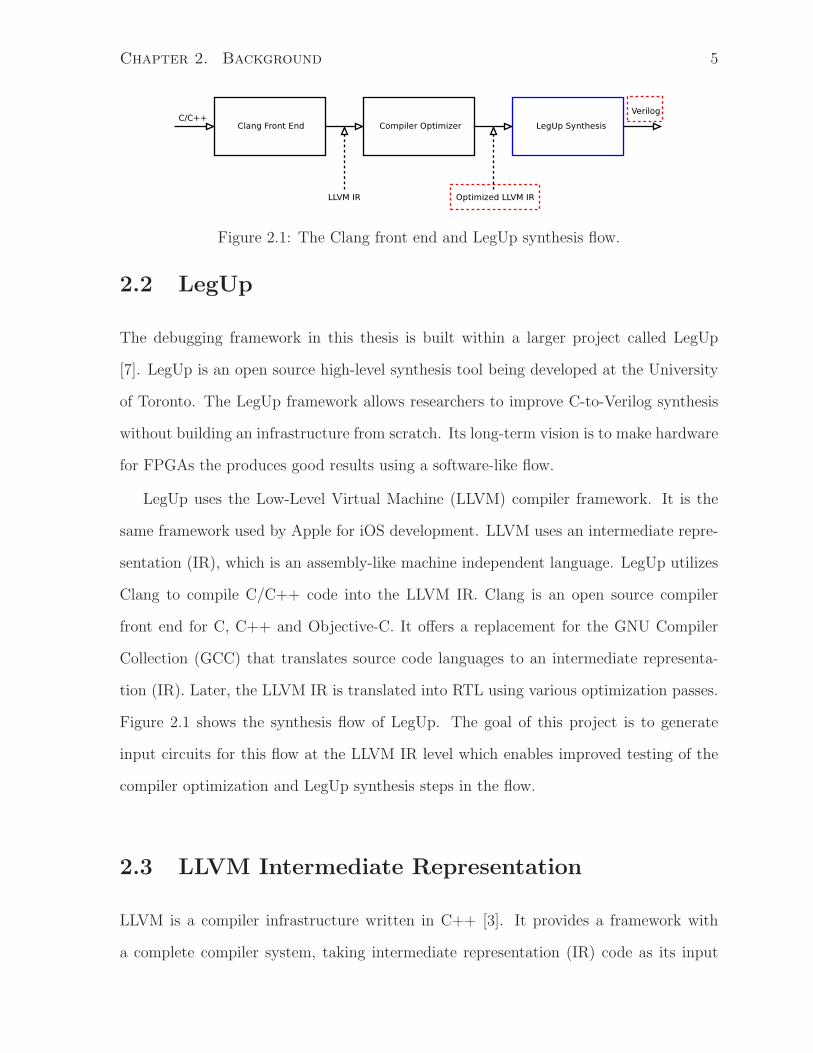
Figure 2.1: The Clang front end and LegUp synthesis flow.
2.2 LegUp
The debugging framework in this thesis is built within a larger project called LegUp
[7]. LegUp is an open source high-level synthesis tool being developed at the University
of Toronto. The LegUp framework allows researchers to improve C-to-Verilog synthesis
without building an infrastructure from scratch. Its long-term vision is to make hardware
for FPGAs the produces good results using a software-like flow.
LegUp uses the Low-Level Virtual Machine (LLVM) compiler framework. It is the
same framework used by Apple for iOS development. LLVM uses an intermediate repre-
sentation (IR), which is an assembly-like machine independent language. LegUp utilizes
Clang to compile C/C++ code into the LLVM IR. Clang is an open source compiler
front end for C, C++ and Objective-C. It offers a replacement for the GNU Compiler
Collection (GCC) that translates source code languages to an intermediate representa-
tion (IR). Later, the LLVM IR is translated into RTL using various optimization passes.
Figure 2.1 shows the synthesis flow of LegUp. The goal of this project is to generate
input circuits for this flow at the LLVM IR level which enables improved testing of the
compiler optimization and LegUp synthesis steps in the flow.
2.3 LLVM Intermediate Representation
LLVM is a compiler infrastructure written in C++ [3]. It provides a framework with
a complete compiler system, taking intermediate representation (IR) code as its input
Chapter 2. Background 6
from a compiler front end and producing an optimized IR. This optimized IR can then
be translated and linked in machine-specific assembly code for a target platform (e.g.
MIPS, x86). LLVM can accept the IR from the GCC tool chain or Clang (used by
LegUp), which allows different compilers to be used with LLVM.
LLVM IR [3] uses static single assignment (SSA) form that provides type safety,
low-level operations, flexibility, and the capability of representing high-level languages
clearly. It is the common code representation used throughout all phases of the LLVM
compilation strategy. It is often written in a file with a .ll file extension. In the case of
LegUp, compilation starts from the LLVM IR level and takes these .ll files as its input.
2.4 Control Flow Graph and Data Flow Graph
2.4.1 Control flow graph (CFG)
A control flow graph (CFG) is a data structure that is built on top of the intermediate
representation to abstract the control flow behaviour of functions [17]. It is a directed
graph where nodes represent basic blocks and edges represent possible control flow from
one basic block (BB) to another. It contains information about a program’s execution
paths and loops. A basic block is a maximal section of straight-line code which can
only be entered via the first instruction of the block and can only be exited via the last
instruction.
2.4.2 Data flow graph (DFG)
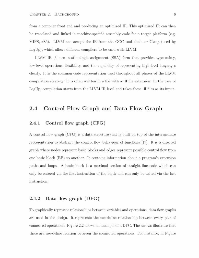
To graphically represent relationships between variables and operations, data flow graphs
are used in the design. It represents the use-define relationship between every pair of
connected operations. Figure 2.2 shows an example of a DFG. The arrows illustrate that
there are use-define relation between the connected operations. For instance, in Figure
Chapter 2. Background 7
Figure 2.2: DFG with use-define chain example.
2.2, the dotted arrow can be described as “the subtracter uses the variable defined by
the adder”.
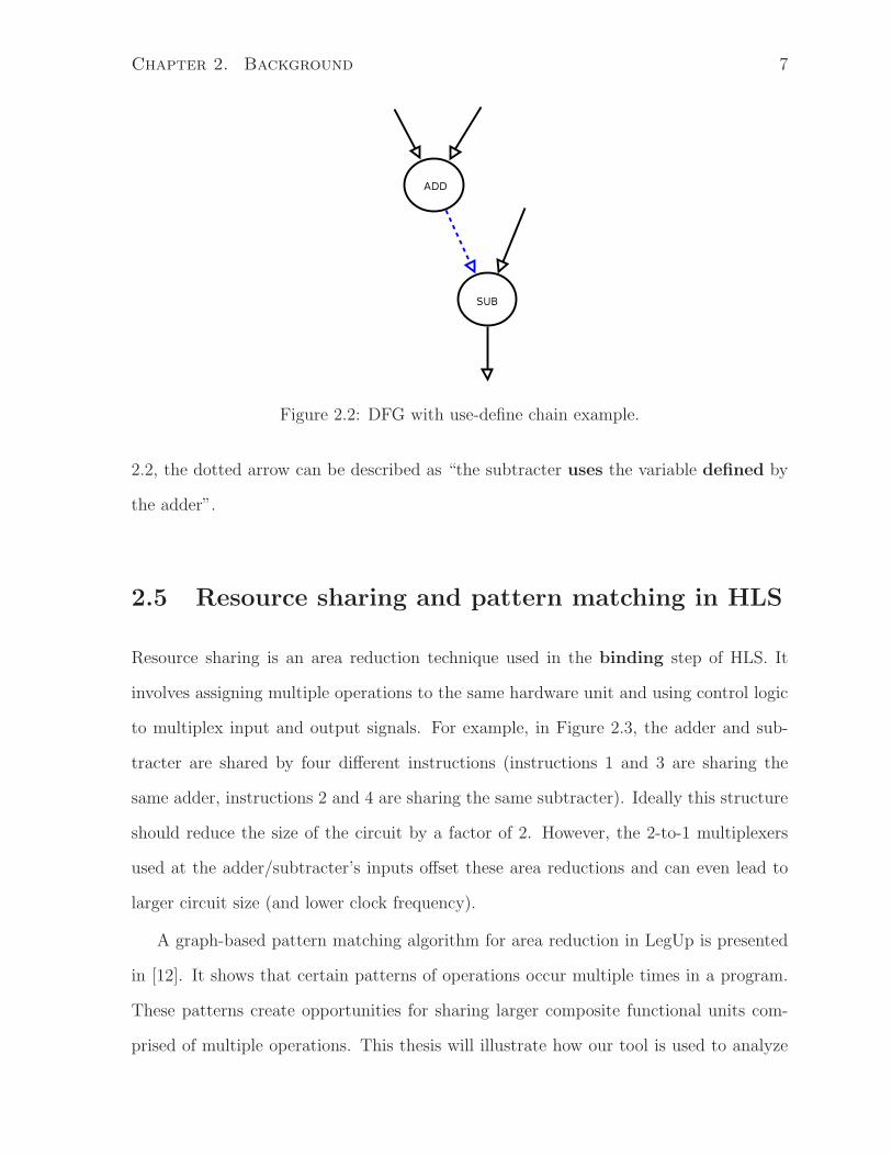
2.5 Resource sharing and pattern matching in HLS
Resource sharing is an area reduction technique used in the binding step of HLS. It
involves assigning multiple operations to the same hardware unit and using control logic
to multiplex input and output signals. For example, in Figure 2.3, the adder and sub-
tracter are shared by four different instructions (instructions 1 and 3 are sharing the
same adder, instructions 2 and 4 are sharing the same subtracter). Ideally this structure
should reduce the size of the circuit by a factor of 2. However, the 2-to-1 multiplexers
used at the adder/subtracter’s inputs offset these area reductions and can even lead to
larger circuit size (and lower clock frequency).
A graph-based pattern matching algorithm for area reduction in LegUp is presented
in [12]. It shows that certain patterns of operations occur multiple times in a program.
These patterns create opportunities for sharing larger composite functional units com-
prised of multiple operations. This thesis will illustrate how our tool is used to analyze
Chapter 2. Background 8
Figure 2.3: Demonstration of resource sharing.
the performance of pattern matching in LegUp.
2.6 Verification techniques for HLS
In this section we describe other existing verification/debugging techniques which are
used for validating HLS tools.
2.6.1 Formal Verification
Formal verification [8] is a method of proving or disproving the validity of a system’s
behaviour by using formal mathematical methods with respect to a set of formal specifi-
cations, constraints or properties. One approach is called model checking, which consists
of an exhaustive exploration of a system’s mathematical model. This requires the system
to be abstracted as a model of a finite state machine with data path (FSMD) described in
some temporal logic expression. With a set of specifications, constraints and properties,
Chapter 2. Background 9
the logic expression can form a boolean equation which is solvable by SAT solvers. On
the other hand, an infinite system model can also be checked by using bounded model
checking (BMC), which bounds the number of states to a limit. For instance, an infinite
loop has to be bounded to a limited number of iterations while translating it to a FSMD.
In terms of verifying high-level synthesis tools, researchers have spent a large amount
of effort on formally verifying correctness of the scheduling process since the input to the
scheduler can be changed in many ways. For example, the control structure of the input
behaviour may be modified by the path-based scheduler [6] as it tries to merge some
consecutive path segments. Also, incorporation of several code-motion techniques [20] in
the scheduling process leads to movements of operations across basic-block boundaries.
These optimizations result in scheduling that does not have a one-to-one correspondence
with the input, which makes the scheduler verification a challenging part of the HLS
verification. A formal method presented in [16] specifically verifies the correctness of the
scheduling process. It uses a finite state machine with data path (FSMD) to represent
both software and hardware schedules in a formal logic format and solves their equivalence
using SAT solvers.
Edmund et al.[8] present a way of using bounded model checking to verify the con-
sistency of behaviours for C and Verilog programs. Given an ANSI-C program and a
Verilog circuit, both are translated into a formula similar to an FSMD that represents
behavioural consistency. The formula is then checked using SAT. Note that the ANSI-C
program and Verilog circuit have no HLS connections. In other words, to verify a cir-
cuit, one has to manually develop a specifically formatted C program that is functionally
equivalent to the Verilog circuit.
Formal methods provide that a tool is correct by using mathematical methods to
check equivalence between hardware and software behaviours. However, there are at
least two disadvantages of this approach. First, formal verification usually involves a
SAT solver which has an exponentially increasing runtime with linearly increasing input
Chapter 2. Background 10
function(){
clock_t A, B;
A = clock();
//
//Some line of instructions to be verified
//
B = clock();
assert((B-A)<100);
}
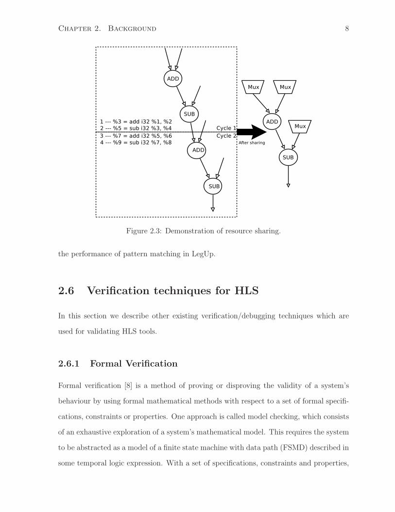
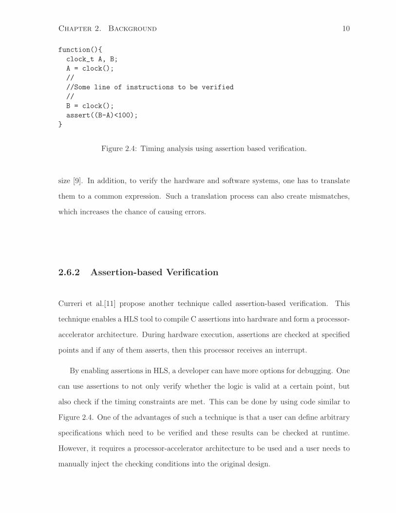
Figure 2.4: Timing analysis using assertion based verification.
size [9]. In addition, to verify the hardware and software systems, one has to translate
them to a common expression. Such a translation process can also create mismatches,
which increases the chance of causing errors.
2.6.2 Assertion-based Verification
Curreri et al.[11] propose another technique called assertion-based verification. This
technique enables a HLS tool to compile C assertions into hardware and form a processor-
accelerator architecture. During hardware execution, assertions are checked at specified
points and if any of them asserts, then this processor receives an interrupt.
By enabling assertions in HLS, a developer can have more options for debugging. One
can use assertions to not only verify whether the logic is valid at a certain point, but
also check if the timing constraints are met. This can be done by using code similar to
Figure 2.4. One of the advantages of such a technique is that a user can define arbitrary
specifications which need to be verified and these results can be checked at runtime.
However, it requires a processor-accelerator architecture to be used and a user needs to
manually inject the checking conditions into the original design.
Chapter 2. Background 11
2.6.3 Manually developed test suites
Manually developed benchmark suites are important for researchers to effectively evaluate
their new ideas and algorithms for HLS. From the late 1980s to the mid 1990s, the HLS
research community had made efforts to develop standard benchmark suites for HLS,
and as a result, two sets of benchmark designs, the High Level Synthesis Workshop 1992
Benchmarks [22] and the 1995 High Level Synthesis Design Repository [21] were released
from the University of California. However, most of these designs were written in VHDL,
and the language for HLS has gradually changed from HDLs to C-based languages.
There were eight benchmarks from the High Level Synthesis Design Repository [21] were
written in C, however they were small programs with less than one hundred lines of
code. These benchmarks can still be useful for studies on loop pipelining and memory
access optimization since these features can be used even in relative small programs.
However, more complex benchmarks are needed to make HLS a practical solution for
larger designs. On the other hand, benchmark programs which are widely used in the field
of computer architecture and compilers are too large and complex for current hardware
synthesis. For instance, C programs in SPEC [4], EEMBC [5], and MediaBench [18] are
not synthesizable even by state-of-the-art HLS tools [14].
LegUp is currently using the CHStone benchmarks as its primary test suite [14], which
is a set of 12 C programs for high-level synthesis. Some key features of the CHStone
benchmarks are as follows:
• CHStone is developed for HLS researchers to analyze the effectiveness and correct-
ness of their new techniques, algorithms, and implementations.
• CHStone consists of 12 programs which are selected from various application do-
mains such as arithmetic, media processing, and security.
• The programs in CHStone are relatively large in terms of source level analysis (e.g.
number of lines of code) and synthesized circuit area.

Chapter 2. Background 12
• All the programs in CHStone have been confirmed to be synthesizable by LegUp
and eXCite (a commercial HLS tool).
• Test vectors are self-contained and no external libraries are necessary.
• CHStone is available to the public.
Our framework is built around LegUp which uses the CHStone as its primary test
suite. We will demonstrate how our tool complements CHStone as a tool for HLS de-
bugging.
Chapter 3
Implementation
This chapter introduces the design architecture of the debugging framework as well as
the detailed implementation algorithms used for each component of the framework.
3.1 Overall debugging flow
To accomplish our goal of automatically generating test cases and verifying HLS tools,
our debugging framework consists of the following steps:
1. Load a configuration file that gives the user-setable parameters for our test gener-
ator.
2. Generate graphs which includes CFGs, DFGs and patterns.
3. Generate LLVM IR from the graphs created in Step 2. This is the test program
that will be executed in software and compiled to hardware.
4. Execute the test program in software with an interpreter to obtain the software
result.
5. Compile the test program to hardware with LegUp to obtain generated RTL.
13
Chapter 3. Implementation 14
6. Simulate the RTL with ModelSim to produce the hardware result.
7. Compare the software and hardware results to verify correctness.
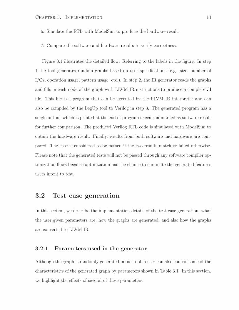
Figure 3.1 illustrates the detailed flow. Referring to the labels in the figure. In step
1 the tool generates random graphs based on user specifications (e.g. size, number of
I/Os, operation usage, pattern usage, etc.). In step 2, the IR generator reads the graphs
and fills in each node of the graph with LLVM IR instructions to produce a complete .ll
file. This file is a program that can be executed by the LLVM IR interpreter and can
also be compiled by the LegUp tool to Verilog in step 3. The generated program has a
single output which is printed at the end of program execution marked as software result
for further comparison. The produced Verilog RTL code is simulated with ModelSim to
obtain the hardware result. Finally, results from both software and hardware are com-
pared. The case is considered to be passed if the two results match or failed otherwise.
Please note that the generated tests will not be passed through any software compiler op-
timization flows because optimization has the chance to eliminate the generated features
users intent to test.
3.2 Test case generation
In this section, we describe the implementation details of the test case generation, what
the user given parameters are, how the graphs are generated, and also how the graphs
are converted to LLVM IR.
3.2.1 Parameters used in the generator
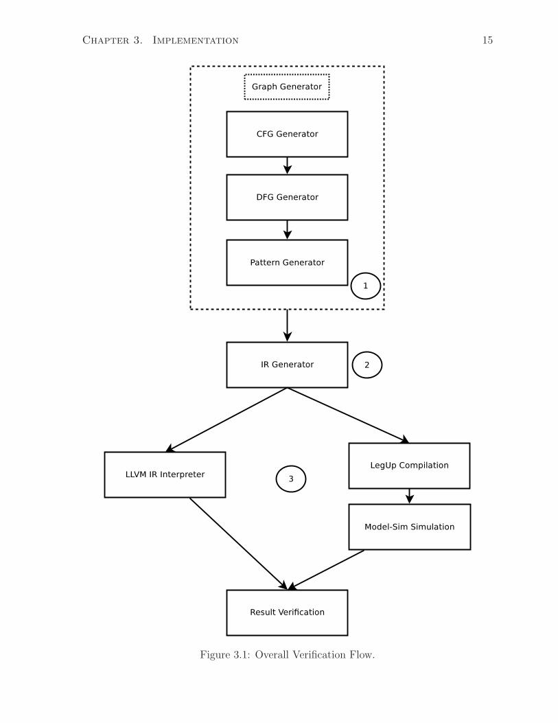
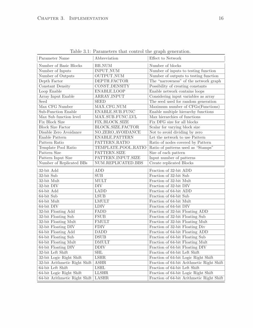
Although the graph is randomly generated in our tool, a user can also control some of the
characteristics of the generated graph by parameters shown in Table 3.1. In this section,
we highlight the effects of several of these parameters.
Chapter 3. Implementation 15
Figure 3.1: Overall Verification Flow.
Chapter 3. Implementation 16
Table 3.1: Parameters that control the graph generation.
Parameter Name Abbreviation Effect to Network
Number of Basic Blocks BB NUM Number of blocksNumber of Inputs INPUT NUM Number of inputs to testing functionNumber of Outputs OUTPUT NUM Number of outputs to testing functionDepth Factor DEPTH FACTOR The “narrowness” of the network graphConstant Density CONST DENSITY Possibility of creating constantsLoop Enable ENABLE LOOP Enable network contains loopsArray Input Enable ARRAY INPUT Considering input variables as arraySeed SEED The seed used for random generationMax CFG Number MAX CFG NUM Maximum number of CFGs(Functions)Sub-Function Enable ENABLE SUB FUNC Enable multiple hierarchy functionsMax Sub function level MAX SUB FUNC LVL Max hierarchies of functionsFix Block Size FIX BLOCK SIZE Fix DFG size for all blocksBlock Size Factor BLOCK SIZE FACTOR Scalar for varying block sizeDisable Zero Avoidance NO ZERO AVOIDANCE Not to avoid dividing by zeroEnable Pattern ENABLE PATTERN Let the network to use PatternPattern Ratio PATTERN RATIO Ratio of nodes covered by PatternTemplate Pool Ratio TEMPLATE POOL RATIO Ratio of patterns used as “Stamps”Pattern Size PATTERN SIZE Size of each patternPattern Input Size PATTERN INPUT SIZE Input number of patternsNumber of Replicated BBs NUM REPLICATED BBS Create replicated Blocks
32-bit Add ADD Fraction of 32-bit ADD32-bit Sub SUB Fraction of 32-bit Sub32-bit Mult MULT Fraction of 32-bit Mult32-bit DIV DIV Fraction of 32-bit DIV64-bit Add LADD Fraction of 64-bit ADD64-bit Sub LSUB Fraction of 64-bit Sub64-bit Mult LMULT Fraction of 64-bit Mult64-bit DIV LDIV Fraction of 64-bit DIV32-bit Floating Add FADD Fraction of 32-bit Floating ADD32-bit Floating Sub FSUB Fraction of 32-bit Floating Sub32-bit Floating Mult FMULT Fraction of 32-bit Floating Mult32-bit Floating DIV FDIV Fraction of 32-bit Floating Div64-bit Floating Add DADD Fraction of 64-bit Floating ADD64-bit Floating Sub DSUB Fraction of 64-bit Floating Sub64-bit Floating Mult DMULT Fraction of 64-bit Floating Mult64-bit Floating DIV DDIV Fraction of 64-bit Floating DIV32-bit Left Shift SHL Fraction of 64-bit Left Shift32-bit Logic Right Shift LSHR Fraction of 64-bit Logic Right Shift32-bit Arithmetic Right Shift ASHR Fraction of 64-bit Arithmetic Right Shift64-bit Left Shift LSHL Fraction of 64-bit Left Shift64-bit Logic Right Shift LLSHR Fraction of 64-bit Logic Right Shift64-bit Arithmetic Right Shift LASHR Fraction of 64-bit Arithmetic Right Shift
Chapter 3. Implementation 17
3.2.1.1 Size control
The parameters that control the size of the generated network are:
• BB NUM. This parameter determines the total number of basic blocks (excluding
the entry and exit blocks) in the top-level CFG. Larger values of this parameter
increase the complexity of the test program, resulting in more branches, loops and
sub-functions.
• INPUT NUM. This parameter specifies the number of input variables for the test-
Func function. testFunc is the top-level test function called by themain wrapper.
If the parameter ARRAY INPUT is set, the input to the function becomes an array
in which the number of elements is equal to INPUT NUM.
• OUTPUT NUM. This parameter specifies the number of output variables returned
by the top-level testFunc function. However, for this function, only a single output
is allowed since only one result is used for the final comparison. User should note
that such a single output constraint is only applicable for the top-level testFunc
function by default. Sub-functions can have multiple returned values and they will
be an array with a number of elements.
• BLOCK SIZE FACTOR. This parameter is a scalar used in Equation: Size of DFG =
BLOCK SIZE FACTOR ∗ (DFG input size+DFG output size) to determine
the number of operations in each DFG. The generator requires this parameter to
be larger than 2 to make sure each input node has at least one connection.
• FIX BLOCK SIZE. By default, the size of a DFG in each basic block varies de-
pending on its number of inputs/outputs and the BLOCK SIZE FACTOR. It can
Chapter 3. Implementation 18
be difficult for a user to control the size of the entire network as the number of in-
puts/outputs are randomly generated for each DFG. By setting the FIX BLOCK SIZE
parameter, the size of each DFG can be fixed.
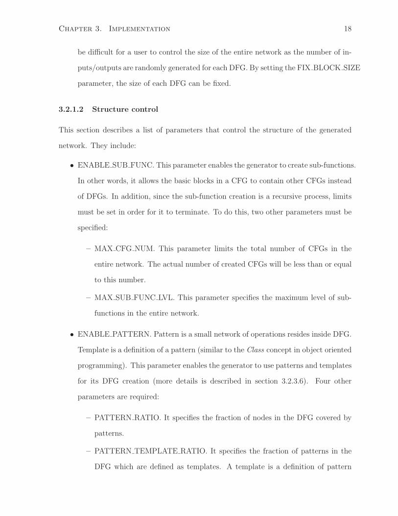
3.2.1.2 Structure control
This section describes a list of parameters that control the structure of the generated
network. They include:
• ENABLE SUB FUNC. This parameter enables the generator to create sub-functions.
In other words, it allows the basic blocks in a CFG to contain other CFGs instead
of DFGs. In addition, since the sub-function creation is a recursive process, limits
must be set in order for it to terminate. To do this, two other parameters must be
specified:
– MAX CFG NUM. This parameter limits the total number of CFGs in the
entire network. The actual number of created CFGs will be less than or equal
to this number.
– MAX SUB FUNC LVL. This parameter specifies the maximum level of sub-
functions in the entire network.
• ENABLE PATTERN. Pattern is a small network of operations resides inside DFG.
Template is a definition of a pattern (similar to the Class concept in object oriented
programming). This parameter enables the generator to use patterns and templates
for its DFG creation (more details is described in section 3.2.3.6). Four other
parameters are required:
– PATTERN RATIO. It specifies the fraction of nodes in the DFG covered by
patterns.
– PATTERN TEMPLATE RATIO. It specifies the fraction of patterns in the
DFG which are defined as templates. A template is a definition of pattern
Chapter 3. Implementation 19
that will be instantiated and placed in the network. The DFG generator
maintains a list of such templates. The size of the template list is given by
PATTERN TEMPLATE RATIO∗ Total number of patterns.
– PATTERN SIZE. It specifies the size of patterns being generated in DFGs.
– PATTERN INPUT SIZE. It specifies the number of inputs to each pattern.
• NUM REPLICATED BBS. This parameter specifies the number of replicated basic
blocks in the network. The reason for having such a parameter is to enable a user
to test functional unit sharing across basic blocks.
• DEPTH FACTOR. This parameter is used in CFG, DFG and pattern generations.
More details about this parameter will be described as we introduce the algorithms
that utilize it. In addition, experiments in Section 4.1 graphically and statistically
show the effects of the DEPTH FACTOR.
3.2.2 Summary of parameters
In this section, we have described parameters that can control the graph generation. To
combine a set of parameters as configuration, a user can use an auto-configuration file
with the argument “-auto-config”. An example of the configuration file is shown in Figure
3.2. This set of parameters tells the generator to create a test program with 10 basic
blocks, 2 scalar input variables, and a single output. The size of each basic block is fixed
with a factor of 10. The operations that can appear in the program are additions and
divisions. They are assigned to equal weights, meaning that the probability for either
operation to appear in the program is the same. In addition, 8 out of the 10 basic blocks
are replications of each other.
Chapter 3. Implementation 20
BB_NUM 10
INPUT_NUM 2
OUTPUT_NUM 1
DEPTH_FACTOR 0.5
ARRAY_INPUT 0
ADD 0.5
DIV 0.5
FIX_BLOCK_SIZE 1
NUM_REPLICATED_BBS 8
BLOCK_SIZE_FACTOR 10
Figure 3.2: An example of a configuration file
3.2.3 Graph generation
3.2.3.1 Graph Structure
In this section, the structure of the generated graph is introduced. The hierarchy of the
network is graphically represented in Figure 3.3. According to the figure, at the highest
level, the tool describes a function as a control flow graph (CFG) which contains the
interactions between basic blocks (BB) (rectangles in Figure 3.3). The CFG has a single
entry and a single exit block. Inside each BB, it either contains a data flow graph (DFG)
or contains another CFG. If it is a CFG, then this CFG is mapped to a sub-function called
by the current function. If a DFG is used, it represents the interconnections between
operations in this BB. Each DFG can have multiple inputs and outputs.
Each DFG is filled by nodes (circles in Figure 3.3) and patterns (highlighted squares in
Figure 3.3). A Node is the smallest representation unit in our structure. It can represent
an operation (add, subtraction, divide, multiplication, etc.), a constant, an input or an
output in the DFG. On the other hand, a pattern is a small network of a fixed number
of operations. The patterns can be stamped into DFGs in order to produce replicated
structures of operations.
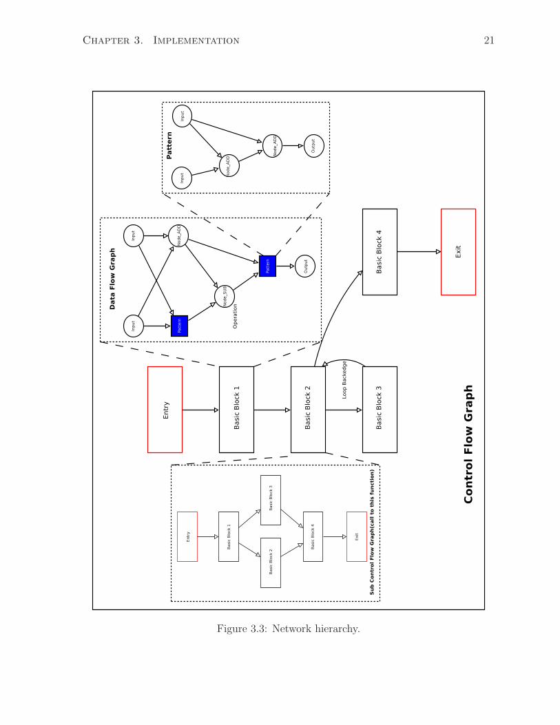
Chapter 3. Implementation 21
Figure 3.3: Network hierarchy.

Chapter 3. Implementation 22
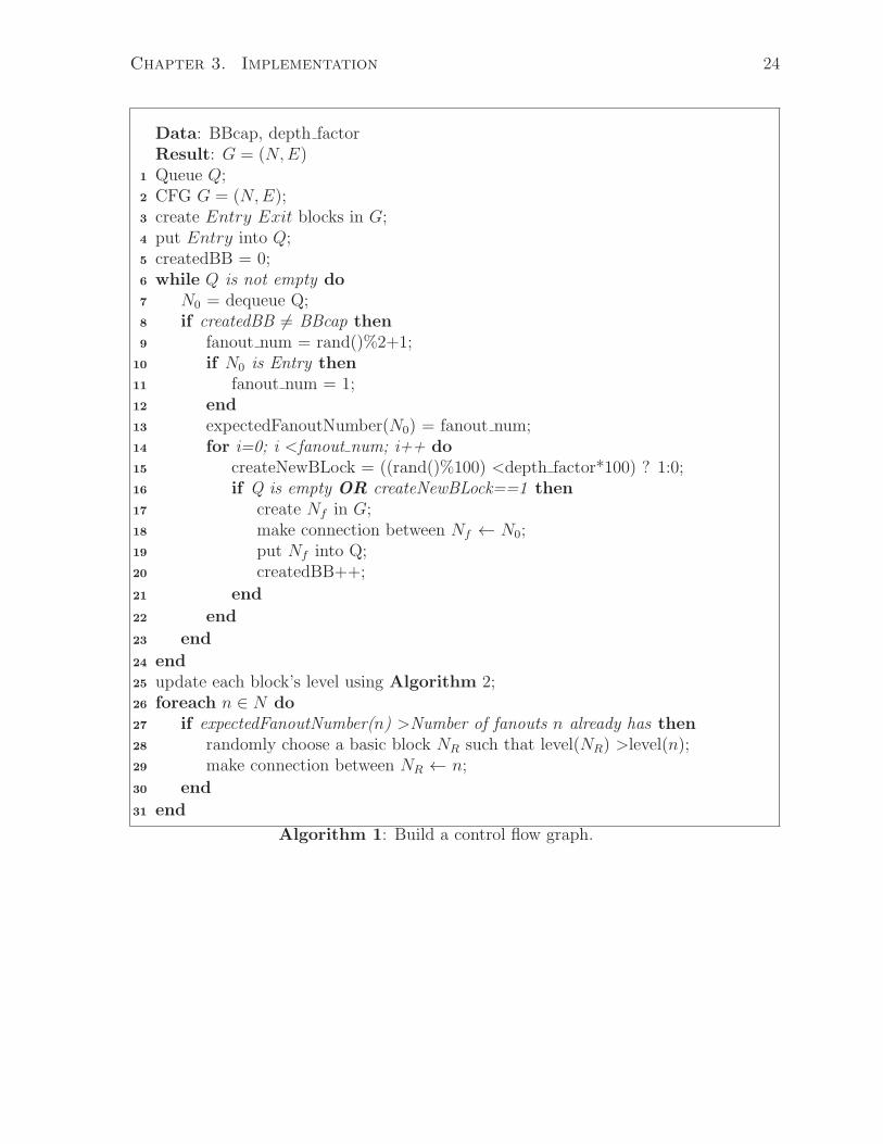
3.2.3.2 CFG generation
The generation starts from the highest level of the graph, which is the control flow graph.
A CFG of a program is a directed graph which can be represented as: G = (N,E). G
represents the graph, N represents a set of basic blocks in the graph and E represents a
set of edges that connect between basic blocks. In addition, an entry block in G is a point
where the graph starts and an exit block in G is a point where the graph ends. Starting
from the entry block, considering it as a root node, the generator builds a network similar
to a breadth-first search traversal using the Algorithm 1. This algorithm is described
below:
1. From line 1 to line 5, the generator initializes a queue and a CFG, creates an entry
and an exit blocks in the CFG and puts the entry block into the queue.
2. From line 6 to line 24, the generator repeats the steps from 3 to 6 below until all
the nodes have been created.
3. The generator takes a block N0 off the queue if the queue is not empty.
4. If the number of created nodes is less than the total number of nodes that needs
to be created (there are more blocks to create), then:
(a) Randomly assign a number to N0. This number represents how many fanouts
N0 has (if N0 is the entry, its fanout number is always 1 for convenience,
otherwise, this value can be either 1 or 2).
(b) If N0 is the last element from the queue, N0 must connect to as least a newly
created node Nf , otherwise the queue will be depleted and the generation
process can not terminate.
(c) Otherwise, for each fanout of N0, depending on the “depth factor” specified
by the user, N0 can either be connected to a newly created node Nf or left as
unconnected. The generator will solve the unconnected points in later steps.

Chapter 3. Implementation 23
(d) If any of N0’s fanout is newly created, put the Nf in the queue.
5. Else if there are no more nodes to create:
(a) Connect N0 to the exit block if there is not a node connected to the exit block
yet.
6. Go back to step 2 until the queue is empty.
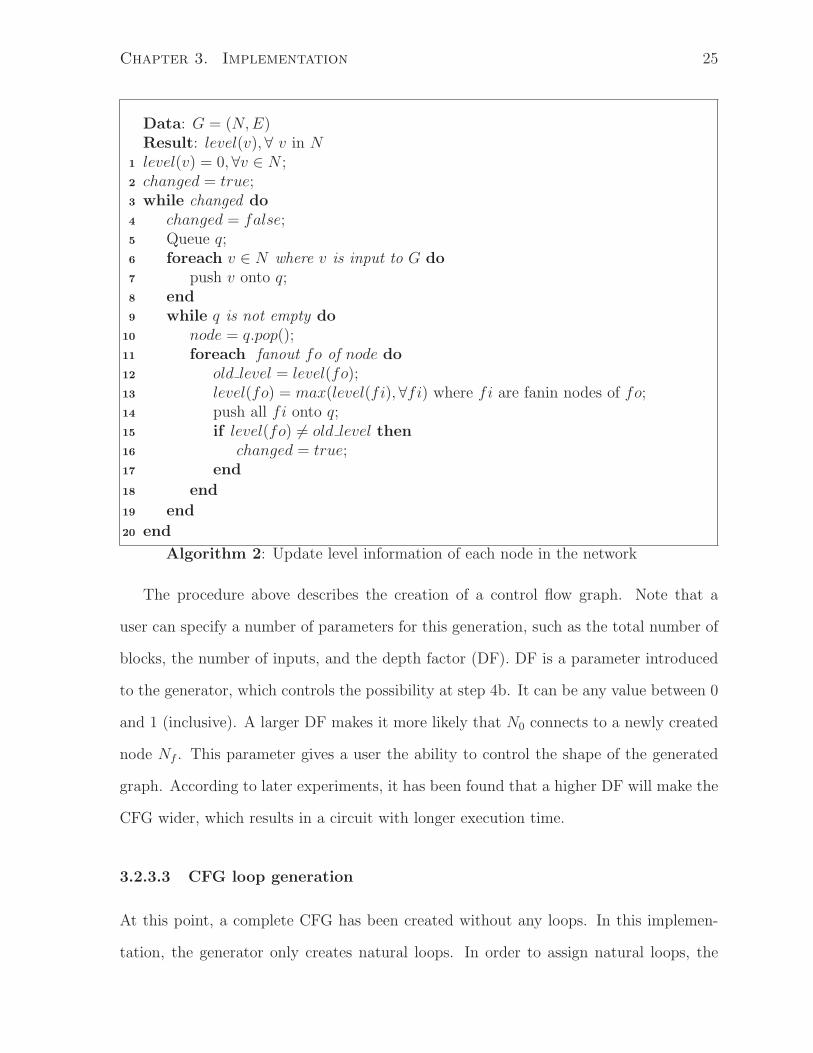
7. At line number 25 of the algorithm, the generator updates the level of each node
using Algorithm 2. A node is assigned to a lower level if it is closer to the input
(e.g. input node is level 0, output node is max level).
8. From line 26 to the end, The generator checks each node, if its expected fanout
number (assigned at step 2a) is less than the number of fanouts it is actually
connected to, randomly assign a node at a higher level as its fanout.
Chapter 3. Implementation 24
Data: BBcap, depth factorResult: G = (N,E)Queue Q;1
CFG G = (N,E);2
create Entry Exit blocks in G;3
put Entry into Q;4
createdBB = 0;5
while Q is not empty do6
N0 = dequeue Q;7
if createdBB 6= BBcap then8
fanout num = rand()%2+1;9
if N0 is Entry then10
fanout num = 1;11
end12
expectedFanoutNumber(N0) = fanout num;13
for i=0; i <fanout num; i++ do14
createNewBLock = ((rand()%100) <depth factor*100) ? 1:0;15
if Q is empty OR createNewBLock==1 then16
create Nf in G;17
make connection between Nf ← N0;18
put Nf into Q;19
createdBB++;20
end21
end22
end23
end24
update each block’s level using Algorithm 2;25
foreach n ∈ N do26
if expectedFanoutNumber(n) >Number of fanouts n already has then27
randomly choose a basic block NR such that level(NR) >level(n);28
make connection between NR ← n;29
end30
end31
Algorithm 1: Build a control flow graph.
Chapter 3. Implementation 25
Data: G = (N,E)Result: level(v), ∀ v in N
level(v) = 0, ∀v ∈ N ;1
changed = true;2
while changed do3
changed = false;4
Queue q;5
foreach v ∈ N where v is input to G do6
push v onto q;7
end8
while q is not empty do9
node = q.pop();10
foreach fanout fo of node do11
old level = level(fo);12
level(fo) = max(level(fi), ∀fi) where fi are fanin nodes of fo;13
push all fi onto q;14
if level(fo) 6= old level then15
changed = true;16
end17
end18
end19
end20
Algorithm 2: Update level information of each node in the network
The procedure above describes the creation of a control flow graph. Note that a
user can specify a number of parameters for this generation, such as the total number of
blocks, the number of inputs, and the depth factor (DF). DF is a parameter introduced
to the generator, which controls the possibility at step 4b. It can be any value between 0
and 1 (inclusive). A larger DF makes it more likely that N0 connects to a newly created
node Nf . This parameter gives a user the ability to control the shape of the generated
graph. According to later experiments, it has been found that a higher DF will make the
CFG wider, which results in a circuit with longer execution time.
3.2.3.3 CFG loop generation
At this point, a complete CFG has been created without any loops. In this implemen-
tation, the generator only creates natural loops. In order to assign natural loops, the
Chapter 3. Implementation 26
generator needs to do an analysis to find all the dominators for each basic block due to
the following reasons [19]:
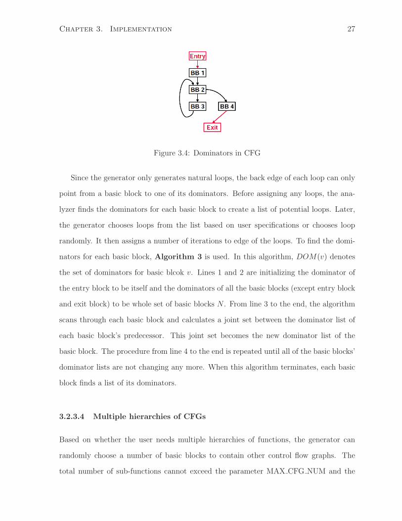
• Dominator: Let G = (N,E) denote a CFG. Let, basic block n, n ⊆ N . n is said to
dominate n, denoted n→ n, iff every path from the entry to n contains n.
– For instance, in Figure 3.4, BB1 → BB1; BB1 → BB2; BB1 → BB3;
BB1 → BB4; BB2 → BB2; BB2 → BB3; BB2 → BB4; BB3 → BB3;
BB4→ BB4.
• A natural loop has a single entry or head node h ⊆ N , where the loop can only be
entered through h. In a program, as long as there is not goto statement, all the
loops are natural.
• A natural loop has an exit or a tail node t ⊆ N .
• Therefore, h has to be a dominator of t.
Data: G = (N,E)Result: DOM(v)∀ v in N
DOM(Entry) = Entry;1
DOM(v) = N∀v ∈ N − (Entry, Exit);2
changed = ture;3
while changed do4
changed = false;5
foreach v ∈ N − (Entry, Exit) do6
oldDOM = DOM(v);7
DOM(v) = N ;8
foreach p ∈ predecessor(v) do9
DOM(v) = DOM(v)⋂DOM(p);10
end11
DOM(v) = DOM(v)⋃v;12
if DOM(v) 6= oldDOM then13
changed = true;14
end15
end16
end17
Algorithm 3: Find dominators for each basic block.
Chapter 3. Implementation 27
Figure 3.4: Dominators in CFG
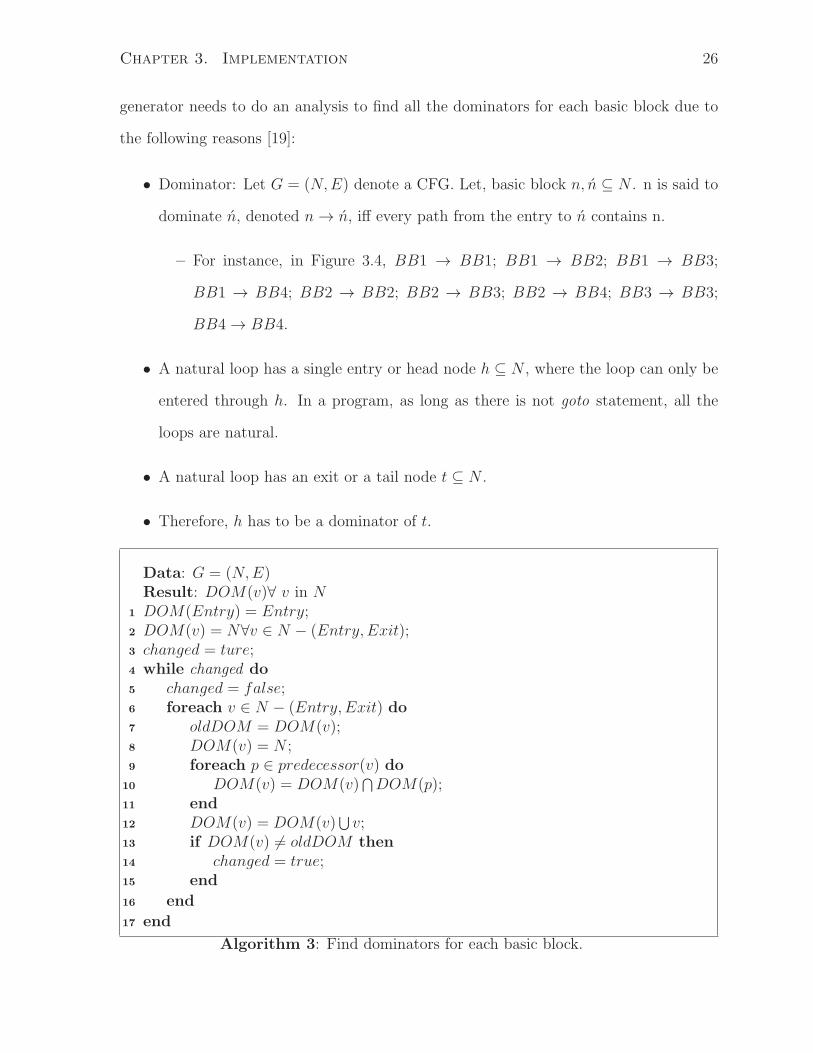
Since the generator only generates natural loops, the back edge of each loop can only
point from a basic block to one of its dominators. Before assigning any loops, the ana-
lyzer finds the dominators for each basic block to create a list of potential loops. Later,
the generator chooses loops from the list based on user specifications or chooses loop
randomly. It then assigns a number of iterations to edge of the loops. To find the domi-
nators for each basic block, Algorithm 3 is used. In this algorithm, DOM(v) denotes
the set of dominators for basic blcok v. Lines 1 and 2 are initializing the dominator of
the entry block to be itself and the dominators of all the basic blocks (except entry block
and exit block) to be whole set of basic blocks N . From line 3 to the end, the algorithm
scans through each basic block and calculates a joint set between the dominator list of
each basic block’s predecessor. This joint set becomes the new dominator list of the
basic block. The procedure from line 4 to the end is repeated until all of the basic blocks’
dominator lists are not changing any more. When this algorithm terminates, each basic
block finds a list of its dominators.
3.2.3.4 Multiple hierarchies of CFGs
Based on whether the user needs multiple hierarchies of functions, the generator can
randomly choose a number of basic blocks to contain other control flow graphs. The
total number of sub-functions cannot exceed the parameter MAX CFG NUM and the
Chapter 3. Implementation 28
maximum level of function calls cannot exceed the parameter MAX SUB FUNC LVL
(a description of all the parameters can be found in Table 3.1). Basic blocks which do
not contain CFGs can be represented by data flow graphs. By going though each BB
(other than the entry and exit blocks), if a BB contains a CFG (based on the definition
of basic block in compiler technology, it cannot contain a function. However, in this
implementation, the definition has been altered and an entire basic block can be mapped
to a CFG in order to enable the sub-function calls), the CFG generator is utilized again
(as discussed since Section 3.2.3.2), otherwise, a DFG generator is called.
3.2.3.5 DFG generation
This section discusses how a data flow graph is generated for each basic block. As shown
in Figure 3.3, a DFG is also a directed, acyclic graph (DAG) that represents the data
transaction network for a portion of a program [19]. A DFG can have multiple input and
output nodes. A DFG is represented as g = (v, e), where v represents a set of nodes, and
e represents a set of directed edges that connect the nodes together to form a network.
In our case, each node in DFG represents either an operation, an input, an output, a
constant, or even a pattern of several operations. Each edge in a DFG represents a data
dependency (use-define relationship) between two connected nodes.
To generate a data flow graph, a user has to specify at least the following parameters:
the number of inputs, the number of outputs, the maximum number of nodes for the
target DFG, the depth factor, and the constant density (a probability parameter that
determines how often constants appear in the DFG network). Once the generator receives
the input parameters, it starts generating the graph using an algorithm similar to the one
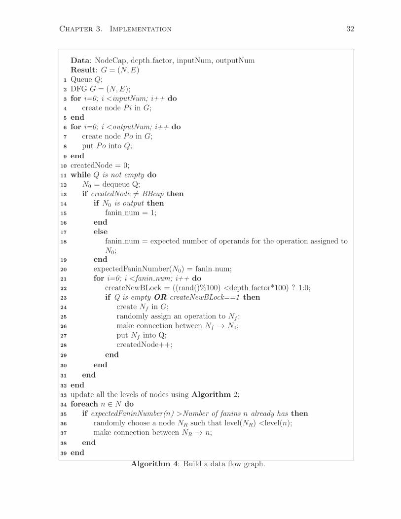
used for CFG generation, a breadth first search-like traversal described in Algorithm 4.
The algorithm is described below:
1. From line 1 to line 9, the DFG generator creates all the input and output nodes
for the graph. In addition, all the output nodes are placed in a queue.
Chapter 3. Implementation 29
Figure 3.5: Assigning operations in the network using a pool of operations.
2. From line 10 to line 32, the generator repeats the steps from 3 to 4 below until the
queue is empty.
3. Dequeue a node N0 from Q. If the number of created nodes is less than the total
number of nodes that need to be created, in other words, there are more nodes to
be created, continue, otherwise go to step 5.
(a) Create connections to the inputs of node N0. Based on the depth factor,
its fan-in points can either be connected to a newly created node or left as
unconnected. If the fan-in node is newly created, put it into Q. Such a node
can be an operation with a randomly assigned operator, a constant with a
random number, or even a pattern.
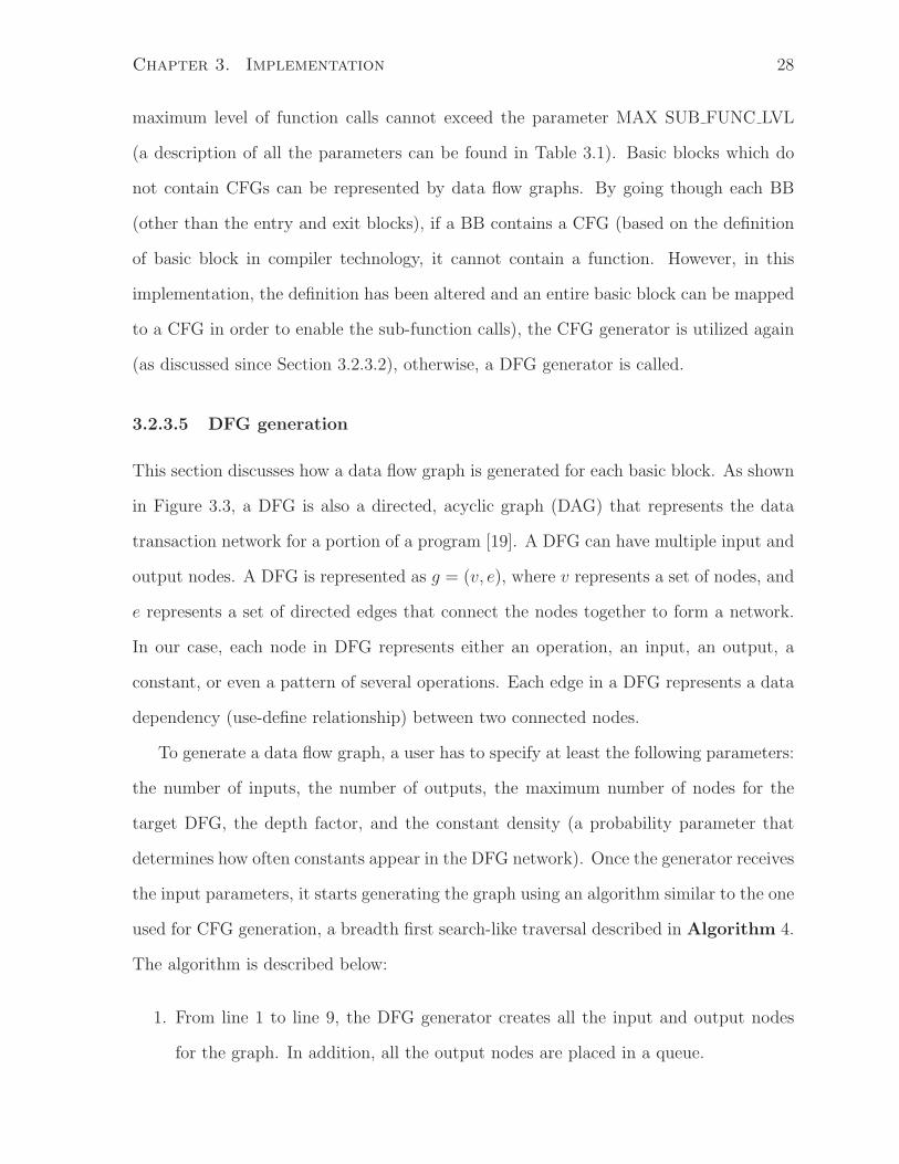
• The probability of a certain operation occurring is determined by their
corresponding fraction factors described in second half of the parameters
shown in Table 3.1. There are two ways of assigning operations.
– The generator assigns operations randomly using the rand() function.
This implementation gives the generated network more randomness.
For instance, if there are only additions and subtractions in the DFG

Chapter 3. Implementation 30
and the user wants them to have equal chance of occurrence, rand()
will generate a number between 1 and 100. The node is assigned to
an addition if the number is less than 50, otherwise a subtraction is
assigned.
– Before the generation starts, the generator creates a pool of all possi-
ble operations, where the size of the pool is the same as the number
of operation nodes. During the creation of the DFG network, a newly
created operation node randomly picks and removes an operation from
the pool, and assigns that operation to the node. Figure 3.5 illustrates
graphically how the operations are picked from the pool and put into
the network. This implementation ensures that the fraction of oc-
currence for each operation exactly matches the user specification.
One should note that the creation of the pool is not random, but the
generator picks operations from the pool randomly.
• The probability of creating a constant is determined by the constant den-
sity factor shown in Table 3.1
4. Repeat step 3 until Q is empty.
5. In line 33, the generator updates the level of each node using Algorithm 2. A node
is assigned to a lower level if it is closer to the inputs.
6. From line 34 to the end, the generator scans through each node, and if there are any
fan-in points left unconnected, randomly assign a node at a lower level (including
input nodes) to that fan-in point.
7. Repeat step 6 until all the nodes have been assigned to a sufficient number of fan-
ins, which is equivalent to the number of inputs of the operation that is assigned
to the node (e.g. an adder should have 2 fan-ins).
Chapter 3. Implementation 31
The procedure above describes the creation of a data flow graph. The depth factor
(DF) in step 3a is a parameter similar to the one used for generating a CFG to control
the shape of the graph.
The test case generator allows the user to choose which operations are to be used in
the test functions. The second half of Table 3.1, shows the operations that are currently
supported in our tool. The value of each parameter has to between 0 and 1 which indicates
the fraction of occurrence for that type of operation. For instance, if a user specifies 0.4
for the addition operation and 0.6 for the subtraction operation, the generator will
generate a network with only these two operations, among which 40% are additions and
60% are subtractions.
Chapter 3. Implementation 32
Data: NodeCap, depth factor, inputNum, outputNumResult: G = (N,E)Queue Q;1
DFG G = (N,E);2
for i=0; i <inputNum; i++ do3
create node Pi in G;4
end5
for i=0; i <outputNum; i++ do6
create node Po in G;7
put Po into Q;8
end9
createdNode = 0;10
while Q is not empty do11
N0 = dequeue Q;12
if createdNode 6= BBcap then13
if N0 is output then14
fanin num = 1;15
end16
else17
fanin num = expected number of operands for the operation assigned to18
N0;end19
expectedFaninNumber(N0) = fanin num;20
for i=0; i <fanin num; i++ do21
createNewBLock = ((rand()%100) <depth factor*100) ? 1:0;22
if Q is empty OR createNewBLock==1 then23
create Nf in G;24
randomly assign an operation to Nf ;25
make connection between Nf → N0;26
put Nf into Q;27
createdNode++;28
end29
end30
end31
end32
update all the levels of nodes using Algorithm 2;33
foreach n ∈ N do34
if expectedFaninNumber(n) >Number of fanins n already has then35
randomly choose a node NR such that level(NR) <level(n);36
make connection between NR → n;37
end38
end39
Algorithm 4: Build a data flow graph.
Chapter 3. Implementation 33
The major differences between the CFG generator and the DFG generator:
• A CFG only has a single input (entry) and a single output (exit).
• Although both generators use breadth first search-like to create networks, the CFG
generator scans from input to output whereas the DFG scans in an opposite direc-
tion for following reasons:
– Scanning from input to output in a CFG gives the generator the ability to
control the number of branches in the network as it always assigns fan-out
numbers to blocks.
– Scanning from output to input in a DFG makes building up the network easier
because the number of inputs to each node is fixed once the type of node is
determined.
• A DFG network has constants. These are the nodes without any fan-ins whereas
in a CFG, the only block without any inputs is the entry block.
• A DFG network has connections between nodes and patterns.
3.2.3.6 Patterns in DFG
As described earlier, a DFG can contain patterns. Our framework implements patterns
as a subclass of nodes as they can co-exist in the same DFG, as shown in Figure 3.3. A
pattern inherits some of the characteristics of a node. They both have fan-in nodes and
fan-out nodes connected to them. In addition, a pattern contains a small network which
consists of a group of nodes (no constants). Using patterns gives a user more control on
the structure of the DFG network. A certain group of patterns can be defined as a set of
stamps. A stamp is a pattern that can potentially be copied and placed elsewhere in the
network. The group of stamps is called the template pool. When the generator creates
the DFG, it can use these stamps to fill out the network, which easily creates replicated
Chapter 3. Implementation 34
structures within the DFG. With these replicated structures, a user can evaluate how
well a HLS tool can detect patterns and create sharable hardware [12].
Parameters PATTERN RATIO and TEMPLATE POOL RATIO are required in or-
der to create patterns in a DFG. The detailed usage of this feature is described in Section
3.2.1.2.
During the process of creating a DFG, if a node is about to be created and determined
to be a pattern, the generator either creates a new pattern and puts it into the template
pool, or selects one of the patterns from the pool to instantiate it and place the instance
into the network. A user can pre-define structures of patterns manually or just specify
the size and the number of inputs/outputs and let the generator create the patterns
randomly. The algorithm for generating random patterns is the similar to generation of
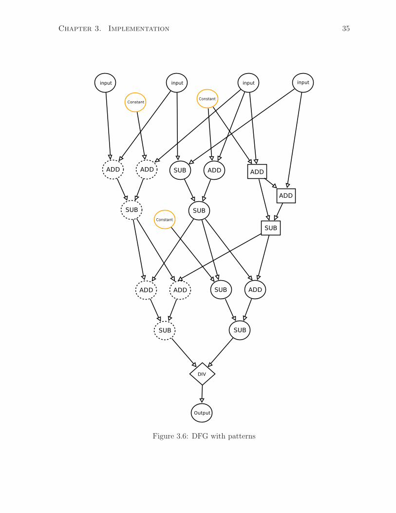
DFGs. Figure 3.6 shows an example of a DFG containing patterns (different patterns are
shown with different shapes: solid circle, dotted circle and solid square). In this graph,
each pattern is of size 3 with 4 inputs and a single output. For instance, the pattern
represented by solid circles has the form of ADD-SUB-ADD, the pattern represented
by dotted circles has the form of SUB-SUB-ADD, and the pattern represented by solid
squares has the form of ADD-ADD-SUB.
After all the DFGs have been generated, a graph that represents the behaviour of a
program has been created. The next step is to interpret this graph and translate it into
a compilable software program.
3.2.4 LLVM IR generation
This section discusses how the test case generator interprets the graph generated from
Section 3.2.3 and finally creates a compilable software program. As LegUp compiles
software from the LLVM IR level, the debugging framework uses the LLVM API to create
a LLVM module to produce a LLVM IR file. A LLVM module represents the top level
structure of the LLVM program. It contains a list of Functions, a list of GlobalVariables,
Chapter 3. Implementation 35
Figure 3.6: DFG with patterns
Chapter 3. Implementation 36
Loop: ;Infinite loop that counts from 0 on up...
%i = phi i32 [ 0, %LoopHeader ], [ %next_i, %Loop ]
%next_i = add i32 %i, 1
br label %Loop
Figure 3.7: An example of PHI instruction in LLVM IR
and a SymbolTable [3].
The CFG at the top level of the hierarchy is translated into a test function named
testFunc. Any CFGs inside it will be considered as sub-functions called by testFunc.
Sub-functions are created recursively by the same routine described in Section 3.2.3.2.
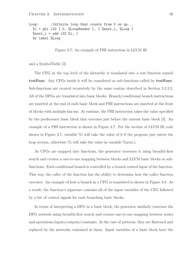
All of the DFGs are translated into basic blocks. Branch/conditional branch instructions
are inserted at the end of each basic block and PHI instructions are inserted at the front
of blocks with multiple fan-ins. At runtime, the PHI instruction takes the value specified
by the predecessor basic block that executes just before the current basic block [3]. An
example of a PHI instruction is shown in Figure 3.7. For the section of LLVM IR code
shown in Figure 3.7, variable %i will take the value of 0 if the program just enters the
loop section, otherwise %i will take the value in variable %next i.
As CFGs are mapped into functions, the generator traverses it using breadth-first
search and creates a one-to-one mapping between blocks and LLVM basic blocks or sub-
functions. Each conditional branch is controlled by a branch control input of the function.
This way, the caller of the function has the ability to determine how the callee function
executes. An example of how a branch in a CFG is translated is shown in Figure 3.8. As
a result, the function’s signature contains all of the input variables of the CFG followed
by a list of control signals for each branching basic blocks.
In terms of interpreting a DFG in a basic block, the generator similarly traverses the
DFG network using breadth-first search and creates one-to-one mapping between nodes
and operations/inputs/outputs/constants. In the case of patterns, they are flattened and
replaced by the networks contained in them. Input variables of a basic block have the
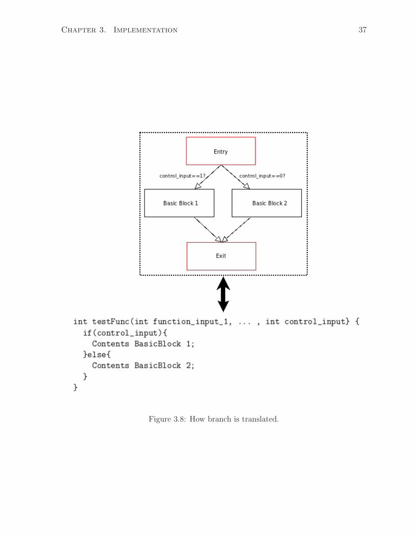
Chapter 3. Implementation 37
Figure 3.8: How branch is translated.
Chapter 3. Implementation 38
%18 = sext i32 %12 to i64
%19 = sext i32 %13 to i64
%20 = add i64 %18, %19
%21 = trunc i64 %20 to i32
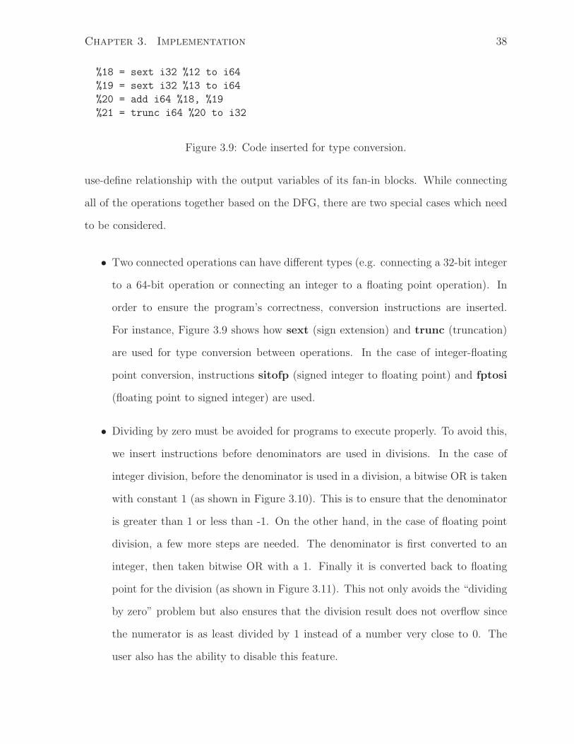
Figure 3.9: Code inserted for type conversion.
use-define relationship with the output variables of its fan-in blocks. While connecting
all of the operations together based on the DFG, there are two special cases which need
to be considered.
• Two connected operations can have different types (e.g. connecting a 32-bit integer
to a 64-bit operation or connecting an integer to a floating point operation). In
order to ensure the program’s correctness, conversion instructions are inserted.
For instance, Figure 3.9 shows how sext (sign extension) and trunc (truncation)
are used for type conversion between operations. In the case of integer-floating
point conversion, instructions sitofp (signed integer to floating point) and fptosi
(floating point to signed integer) are used.
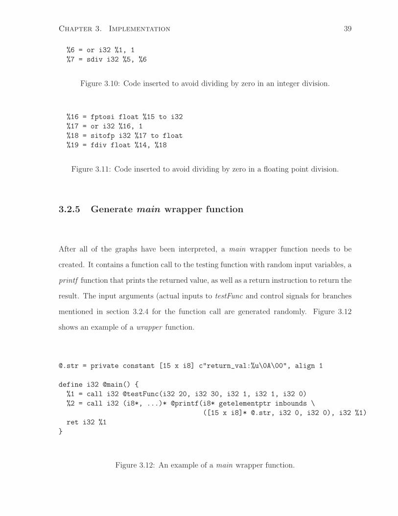
• Dividing by zero must be avoided for programs to execute properly. To avoid this,
we insert instructions before denominators are used in divisions. In the case of
integer division, before the denominator is used in a division, a bitwise OR is taken
with constant 1 (as shown in Figure 3.10). This is to ensure that the denominator
is greater than 1 or less than -1. On the other hand, in the case of floating point
division, a few more steps are needed. The denominator is first converted to an
integer, then taken bitwise OR with a 1. Finally it is converted back to floating
point for the division (as shown in Figure 3.11). This not only avoids the “dividing
by zero” problem but also ensures that the division result does not overflow since
the numerator is as least divided by 1 instead of a number very close to 0. The
user also has the ability to disable this feature.
Chapter 3. Implementation 39
%6 = or i32 %1, 1
%7 = sdiv i32 %5, %6
Figure 3.10: Code inserted to avoid dividing by zero in an integer division.
%16 = fptosi float %15 to i32
%17 = or i32 %16, 1
%18 = sitofp i32 %17 to float
%19 = fdiv float %14, %18
Figure 3.11: Code inserted to avoid dividing by zero in a floating point division.
3.2.5 Generate main wrapper function
After all of the graphs have been interpreted, a main wrapper function needs to be
created. It contains a function call to the testing function with random input variables, a
printf function that prints the returned value, as well as a return instruction to return the
result. The input arguments (actual inputs to testFunc and control signals for branches
mentioned in section 3.2.4 for the function call are generated randomly. Figure 3.12
shows an example of a wrapper function.
@.str = private constant [15 x i8] c"return_val:%u\0A\00", align 1
define i32 @main() {
%1 = call i32 @testFunc(i32 20, i32 30, i32 1, i32 1, i32 0)
%2 = call i32 (i8*, ...)* @printf(i8* getelementptr inbounds \
([15 x i8]* @.str, i32 0, i32 0), i32 %1)
ret i32 %1
}
Figure 3.12: An example of a main wrapper function.
Chapter 3. Implementation 40
3.3 HW/SW results verification and Analysis
Up to this point, a compilable LLVM IR program has been created which has the post-
fix .ll. Recall in Figure 3.1, the IR program is executed by the LLVM IR interpreter.
The printf function in the main wrapper provides a final result marked as the software
result. On the other hand, the IR is compiled by a HLS tool (LegUp in this case) to a
Verilog file. This Verilog file contains the generated RTL including a test bench so that
it can be directly simulated by ModelSim. As LegUp compiles the printf functions into
the display function in Verilog, the final simulation result is produced and marked as
the hardware result. Finally, if both the hardware result and software result match, this
test case is marked as a pass, otherwise a fail. Furthermore, the produced hardware can
also be synthesized using Quartus to gather additional hardware statistics (circuit size,
circuit speed).
3.4 Summary
This chapter has introduced the implementation details of our auto test case generator. It
described the algorithms which are used to generate control flow graphs, data flow graphs
and loops, and also described how to translate the generated graphs into executable
programs. It also explained the uses of the different parameters which control how the
graphs are generated. In addition, it illustrated how each test case is verified.
Chapter 4
Experiments
In order to evaluate the novelty and the usefulness of this framework, we have developed
several different experiments. This chapter describes each experiment with results.
4.1 Effect of depth factor
The depth factor is a parameter that is used in all of the CFG, DFG, and pattern
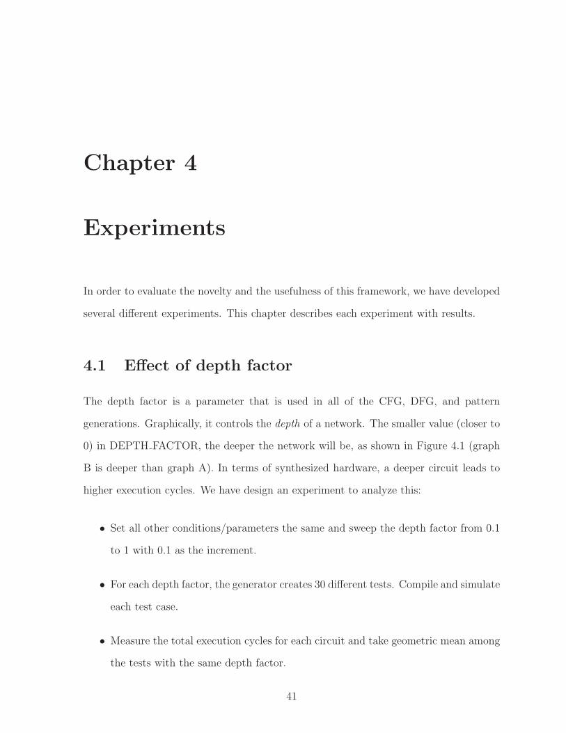
generations. Graphically, it controls the depth of a network. The smaller value (closer to
0) in DEPTH FACTOR, the deeper the network will be, as shown in Figure 4.1 (graph
B is deeper than graph A). In terms of synthesized hardware, a deeper circuit leads to
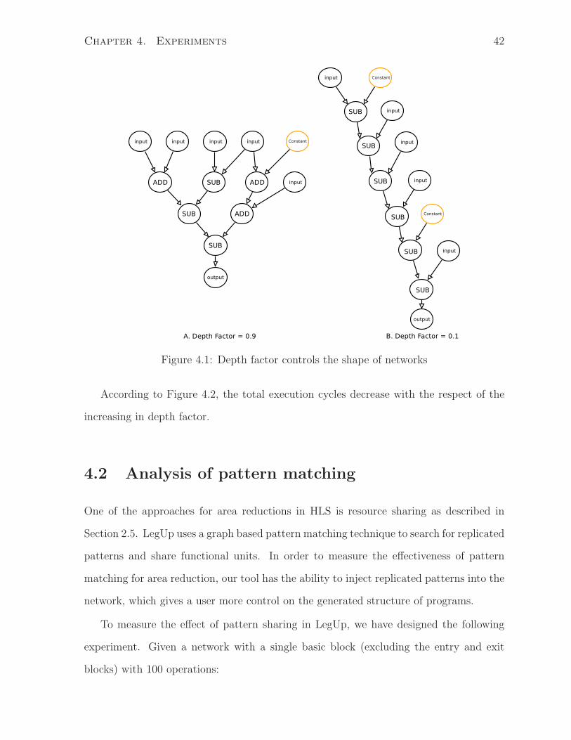
higher execution cycles. We have design an experiment to analyze this:
• Set all other conditions/parameters the same and sweep the depth factor from 0.1
to 1 with 0.1 as the increment.
• For each depth factor, the generator creates 30 different tests. Compile and simulate
each test case.
• Measure the total execution cycles for each circuit and take geometric mean among
the tests with the same depth factor.
41
Chapter 4. Experiments 42
Figure 4.1: Depth factor controls the shape of networks
According to Figure 4.2, the total execution cycles decrease with the respect of the
increasing in depth factor.
4.2 Analysis of pattern matching
One of the approaches for area reductions in HLS is resource sharing as described in
Section 2.5. LegUp uses a graph based pattern matching technique to search for replicated
patterns and share functional units. In order to measure the effectiveness of pattern
matching for area reduction, our tool has the ability to inject replicated patterns into the
network, which gives a user more control on the generated structure of programs.
To measure the effect of pattern sharing in LegUp, we have designed the following
experiment. Given a network with a single basic block (excluding the entry and exit
blocks) with 100 operations:
Chapter 4. Experiments 43
Figure 4.2: Depth Factor controls total execution cycles of circuits
• Set the PATTERN RATIO to 1. This tells the generator that 100% of nodes in
the basic block should be covered by patterns.
• Set the FIX BLOCK SIZE to 1 to make sure all the generated test cases have the
same number of operations.
• Gradually increase the TEMPLATE POOL RATIO from 0 to 1, with 0.1 incre-
ments each time (0 indicates all of the patterns in the DFG are different. As the
parameter is increased, the number of replicated patterns increase. Finally, when
the value equals 1, it makes the entire DFG covered by a single pattern). For each
value of this parameter, the tool generates 30 different test cases and uses LegUp
and Quartus II to synthesize them.
• Collect the area of circuits for each test case while grouping circuits generated from
the same TEMPLATE POOL RATIO as a set.
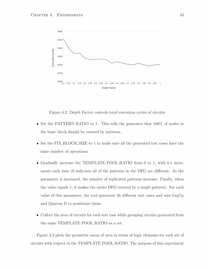
Figure 4.3 plots the geometric mean of area in terms of logic elements for each set of
circuits with respect to the TEMPLATE POOL RATIO. The purpose of this experiment
Chapter 4. Experiments 44
Figure 4.3: Resource sharability of replicated patterns within one BB.
is to find out how much area can be reduced as we inject more potential sharable patterns.
However, according to Figure 4.3, the area of circuit does not necessarily have a linear
relationship with the TEMPLATE POOL RATIO. Base on the log files produced by
LegUp, those injected patterns cannot always be found by LegUp. These suggest that
the current pattern matching algorithm in LegUp can be altered to further reduce the
circuit area.
4.3 An alternative binding algorithm
The experiment described in the previous section implies that the area of the synthesized
circuit does not necessarily decrease as the number replicated patterns increases with
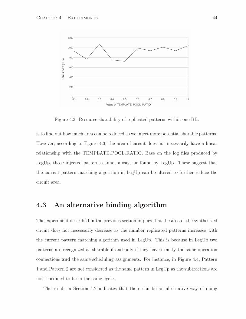
the current pattern matching algorithm used in LegUp. This is because in LegUp two
patterns are recognized as sharable if and only if they have exactly the same operation
connections and the same scheduling assignments. For instance, in Figure 4.4, Pattern
1 and Pattern 2 are not considered as the same pattern in LegUp as the subtractions are
not scheduled to be in the same cycle.
The result in Section 4.2 indicates that there can be an alternative way of doing
Chapter 4. Experiments 45
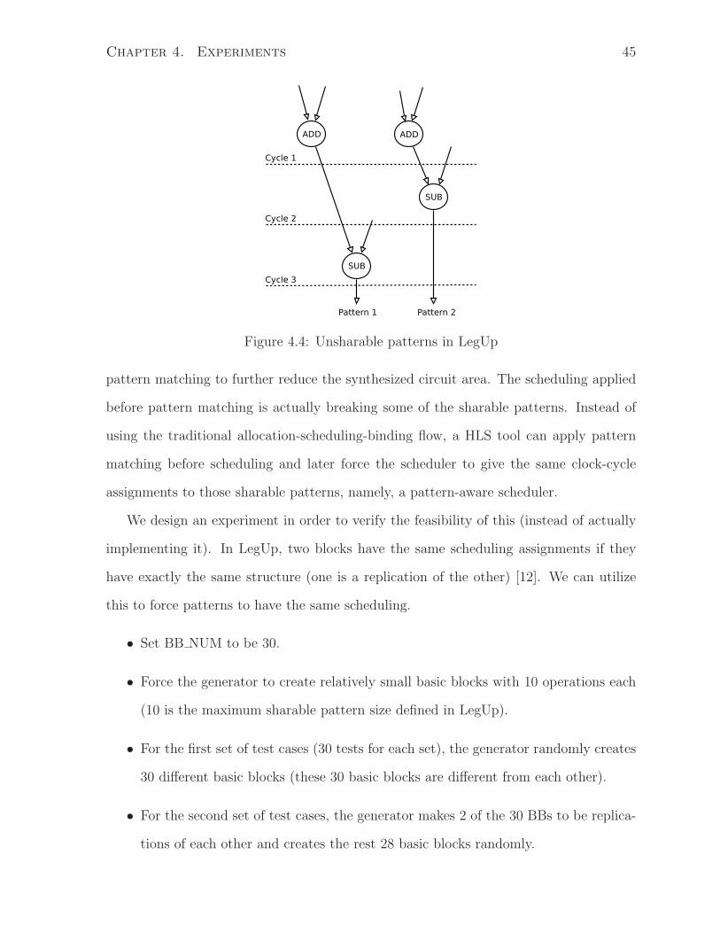
Figure 4.4: Unsharable patterns in LegUp
pattern matching to further reduce the synthesized circuit area. The scheduling applied
before pattern matching is actually breaking some of the sharable patterns. Instead of
using the traditional allocation-scheduling-binding flow, a HLS tool can apply pattern
matching before scheduling and later force the scheduler to give the same clock-cycle
assignments to those sharable patterns, namely, a pattern-aware scheduler.
We design an experiment in order to verify the feasibility of this (instead of actually
implementing it). In LegUp, two blocks have the same scheduling assignments if they
have exactly the same structure (one is a replication of the other) [12]. We can utilize
this to force patterns to have the same scheduling.
• Set BB NUM to be 30.
• Force the generator to create relatively small basic blocks with 10 operations each
(10 is the maximum sharable pattern size defined in LegUp).
• For the first set of test cases (30 tests for each set), the generator randomly creates
30 different basic blocks (these 30 basic blocks are different from each other).
• For the second set of test cases, the generator makes 2 of the 30 BBs to be replica-
tions of each other and creates the rest 28 basic blocks randomly.
Chapter 4. Experiments 46
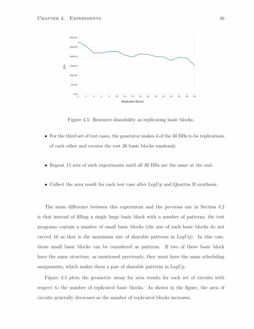
Figure 4.5: Resource sharability as replicating basic blocks.
• For the third set of test cases, the generator makes 4 of the 30 BBs to be replications
of each other and creates the rest 26 basic blocks randomly.
• Repeat 15 sets of such experiments until all 30 BBs are the same at the end.
• Collect the area result for each test case after LegUp and Quartus II synthesis.
The main difference between this experiment and the previous one in Section 4.2
is that instead of filling a single large basic block with a number of patterns, the test
programs contain a number of small basic blocks (the size of such basic blocks do not
exceed 10 as that is the maximum size of sharable patterns in LegUp). In this case,
those small basic blocks can be considered as patterns. If two of these basic block
have the same structure, as mentioned previously, they must have the same scheduling
assignments, which makes them a pair of sharable patterns in LegUp.
Figure 4.5 plots the geometric mean for area results for each set of circuits with
respect to the number of replicated basic blocks. As shown in the figure, the area of
circuits generally decreases as the number of replicated blocks increases.
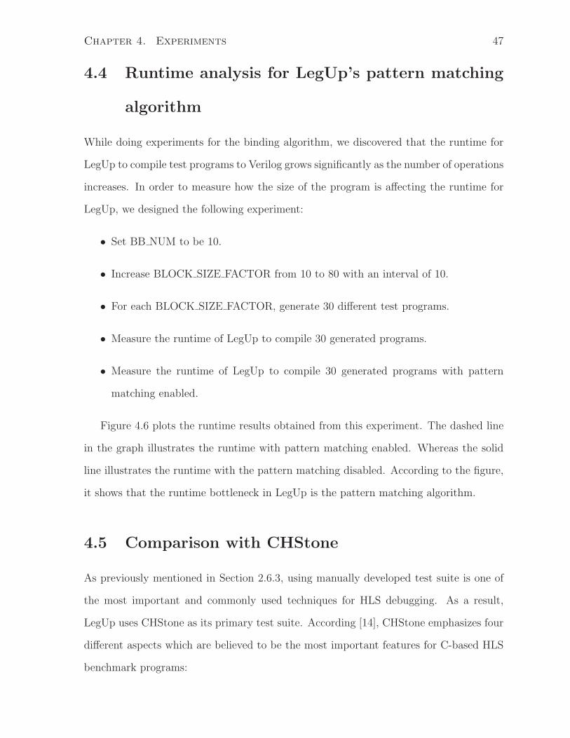
Chapter 4. Experiments 47
4.4 Runtime analysis for LegUp’s pattern matching
algorithm
While doing experiments for the binding algorithm, we discovered that the runtime for
LegUp to compile test programs to Verilog grows significantly as the number of operations
increases. In order to measure how the size of the program is affecting the runtime for
LegUp, we designed the following experiment:
• Set BB NUM to be 10.
• Increase BLOCK SIZE FACTOR from 10 to 80 with an interval of 10.
• For each BLOCK SIZE FACTOR, generate 30 different test programs.
• Measure the runtime of LegUp to compile 30 generated programs.
• Measure the runtime of LegUp to compile 30 generated programs with pattern
matching enabled.
Figure 4.6 plots the runtime results obtained from this experiment. The dashed line
in the graph illustrates the runtime with pattern matching enabled. Whereas the solid
line illustrates the runtime with the pattern matching disabled. According to the figure,
it shows that the runtime bottleneck in LegUp is the pattern matching algorithm.
4.5 Comparison with CHStone
As previously mentioned in Section 2.6.3, using manually developed test suite is one of
the most important and commonly used techniques for HLS debugging. As a result,
LegUp uses CHStone as its primary test suite. According [14], CHStone emphasizes four
different aspects which are believed to be the most important features for C-based HLS
benchmark programs:
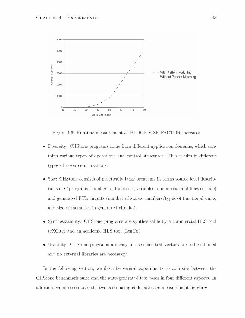
Chapter 4. Experiments 48
Figure 4.6: Runtime measurement as BLOCK SIZE FACTOR increases
• Diversity: CHStone programs come from different application domains, which con-
tains various types of operations and control structures. This results in different
types of resource utilizations.
• Size: CHStone consists of practically large programs in terms source level descrip-
tions of C programs (numbers of functions, variables, operations, and lines of code)
and generated RTL circuits (number of states, numbers/types of functional units,
and size of memories in generated circuits).
• Synthesizability: CHStone programs are synthesizable by a commercial HLS tool
(eXCite) and an academic HLS tool (LegUp).
• Usability: CHStone programs are easy to use since test vectors are self-contained
and no external libraries are necessary.
In the following section, we describe several experiments to compare between the
CHStone benchmark suite and the auto-generated test cases in four different aspects. In
addition, we also compare the two cases using code coverage measurement by gcov.
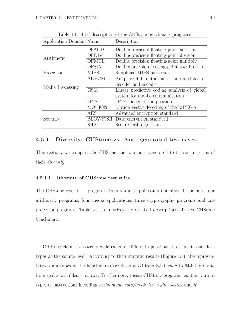
Chapter 4. Experiments 49
Table 4.1: Brief description of the CHStone benchmark programs.
Application Domain Name Description
Arithmetic
DFADD Double precision floating-point additionDFDIV Double precision floating-point divisionDFMUL Double precision floating-point multiplyDFSIN Double precision floating-point sine function
Processor MIPS Simplified MIPS processor
Media Processing
ADPCM Adaptive differential pulse code modulationdecoder and encoder
GSM Linear predictive coding analysis of globalsystem for mobile communication
JPEG JPEG image decompressionMOTION Motion vector decoding of the MPEG-2
SecurityAES Advanced encryption standardBLOWFISH Data encryption standardSHA Secure hash algorithm
4.5.1 Diversity: CHStone vs. Auto-generated test cases
This section, we compare the CHStone and our auto-generated test cases in terms of
their diversity.
4.5.1.1 Diversity of CHStone test suite
The CHStone selects 12 programs from various application domains. It includes four
arithmetic programs, four media applications, three cryptography programs and one
processor program. Table 4.1 summarizes the detailed descriptions of each CHStone
benchmark.
CHStone claims to cover a wide range of different operations, statements and data
types at the source level. According to their statistic results (Figure 4.7), the represen-
tative data types of the benchmarks are distributed from 8-bit char to 64-bit int, and
from scalar variables to arrays. Furthermore, theses CHStone programs contain various
types of instructions including assignment, goto/break, for, while, switch and if
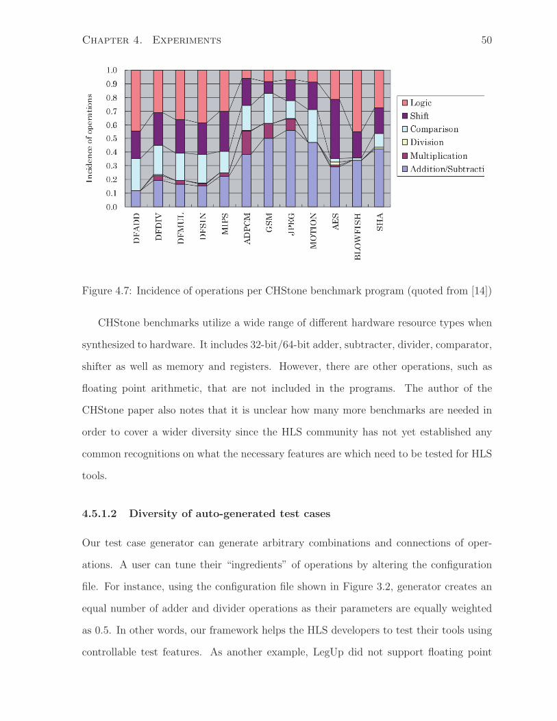
Chapter 4. Experiments 50
Figure 4.7: Incidence of operations per CHStone benchmark program (quoted from [14])
CHStone benchmarks utilize a wide range of different hardware resource types when
synthesized to hardware. It includes 32-bit/64-bit adder, subtracter, divider, comparator,
shifter as well as memory and registers. However, there are other operations, such as
floating point arithmetic, that are not included in the programs. The author of the
CHStone paper also notes that it is unclear how many more benchmarks are needed in
order to cover a wider diversity since the HLS community has not yet established any
common recognitions on what the necessary features are which need to be tested for HLS
tools.
4.5.1.2 Diversity of auto-generated test cases
Our test case generator can generate arbitrary combinations and connections of oper-
ations. A user can tune their “ingredients” of operations by altering the configuration
file. For instance, using the configuration file shown in Figure 3.2, generator creates an
equal number of adder and divider operations as their parameters are equally weighted
as 0.5. In other words, our framework helps the HLS developers to test their tools using
controllable test features. As another example, LegUp did not support floating point
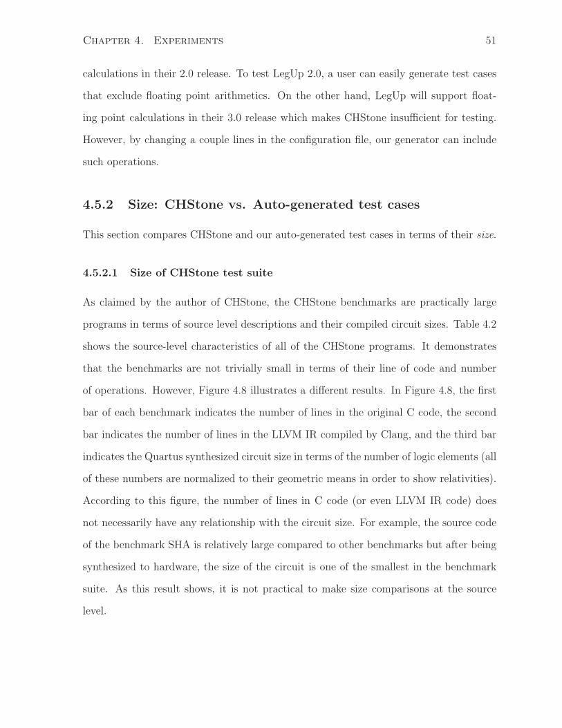
Chapter 4. Experiments 51
calculations in their 2.0 release. To test LegUp 2.0, a user can easily generate test cases
that exclude floating point arithmetics. On the other hand, LegUp will support float-
ing point calculations in their 3.0 release which makes CHStone insufficient for testing.
However, by changing a couple lines in the configuration file, our generator can include
such operations.
4.5.2 Size: CHStone vs. Auto-generated test cases
This section compares CHStone and our auto-generated test cases in terms of their size.
4.5.2.1 Size of CHStone test suite
As claimed by the author of CHStone, the CHStone benchmarks are practically large
programs in terms of source level descriptions and their compiled circuit sizes. Table 4.2
shows the source-level characteristics of all of the CHStone programs. It demonstrates
that the benchmarks are not trivially small in terms of their line of code and number
of operations. However, Figure 4.8 illustrates a different results. In Figure 4.8, the first
bar of each benchmark indicates the number of lines in the original C code, the second
bar indicates the number of lines in the LLVM IR compiled by Clang, and the third bar
indicates the Quartus synthesized circuit size in terms of the number of logic elements (all
of these numbers are normalized to their geometric means in order to show relativities).
According to this figure, the number of lines in C code (or even LLVM IR code) does
not necessarily have any relationship with the circuit size. For example, the source code
of the benchmark SHA is relatively large compared to other benchmarks but after being
synthesized to hardware, the size of the circuit is one of the smallest in the benchmark
suite. As this result shows, it is not practical to make size comparisons at the source
level.
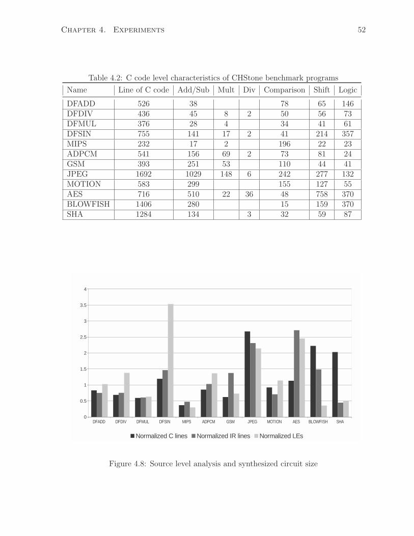
Chapter 4. Experiments 52
Table 4.2: C code level characteristics of CHStone benchmark programs
Name Line of C code Add/Sub Mult Div Comparison Shift Logic
DFADD 526 38 78 65 146DFDIV 436 45 8 2 50 56 73DFMUL 376 28 4 34 41 61DFSIN 755 141 17 2 41 214 357MIPS 232 17 2 196 22 23ADPCM 541 156 69 2 73 81 24GSM 393 251 53 110 44 41JPEG 1692 1029 148 6 242 277 132MOTION 583 299 155 127 55AES 716 510 22 36 48 758 370BLOWFISH 1406 280 15 159 370SHA 1284 134 3 32 59 87
Figure 4.8: Source level analysis and synthesized circuit size
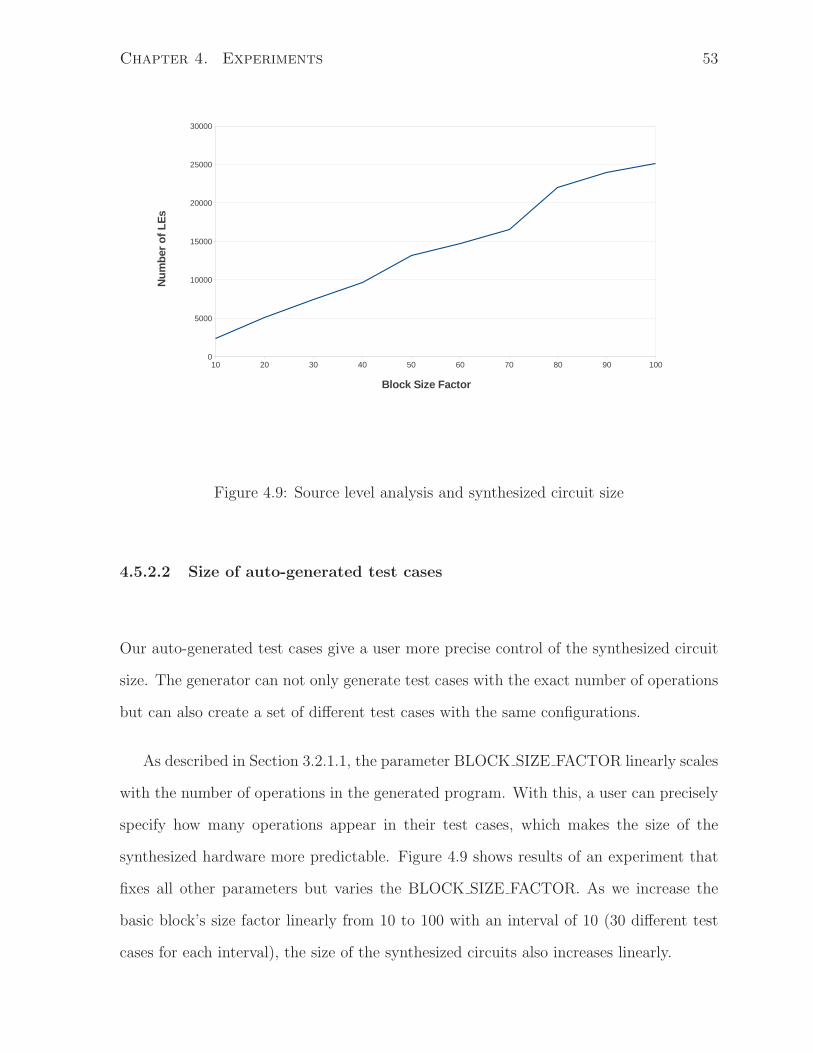
Chapter 4. Experiments 53
Figure 4.9: Source level analysis and synthesized circuit size
4.5.2.2 Size of auto-generated test cases
Our auto-generated test cases give a user more precise control of the synthesized circuit
size. The generator can not only generate test cases with the exact number of operations
but can also create a set of different test cases with the same configurations.
As described in Section 3.2.1.1, the parameter BLOCK SIZE FACTOR linearly scales
with the number of operations in the generated program. With this, a user can precisely
specify how many operations appear in their test cases, which makes the size of the
synthesized hardware more predictable. Figure 4.9 shows results of an experiment that
fixes all other parameters but varies the BLOCK SIZE FACTOR. As we increase the
basic block’s size factor linearly from 10 to 100 with an interval of 10 (30 different test
cases for each interval), the size of the synthesized circuits also increases linearly.
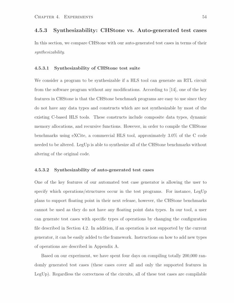
Chapter 4. Experiments 54
4.5.3 Synthesizability: CHStone vs. Auto-generated test cases
In this section, we compare CHStone with our auto-generated test cases in terms of their
synthesizability.
4.5.3.1 Synthesizability of CHStone test suite
We consider a program to be synthesizable if a HLS tool can generate an RTL circuit
from the software program without any modifications. According to [14], one of the key
features in CHStone is that the CHStone benchmark programs are easy to use since they
do not have any data types and constructs which are not synthesizable by most of the
existing C-based HLS tools. These constructs include composite data types, dynamic
memory allocations, and recursive functions. However, in order to compile the CHStone
benchmarks using eXCite, a commercial HLS tool, approximately 3.0% of the C code
needed to be altered. LegUp is able to synthesize all of the CHStone benchmarks without
altering of the original code.
4.5.3.2 Synthesizability of auto-generated test cases
One of the key features of our automated test case generator is allowing the user to
specify which operations/structures occur in the test programs. For instance, LegUp
plans to support floating point in their next release, however, the CHStone benchmarks
cannot be used as they do not have any floating point data types. In our tool, a user
can generate test cases with specific types of operations by changing the configuration
file described in Section 4.2. In addition, if an operation is not supported by the current
generator, it can be easily added to the framework. Instructions on how to add new types
of operations are described in Appendix A.
Based on our experiment, we have spent four days on compiling totally 200,000 ran-
domly generated test cases (these cases cover all and only the supported features in
LegUp). Regardless the correctness of the circuits, all of these test cases are compilable
Chapter 4. Experiments 55
printf ("Result: %d\n", main_result);
if (main_result == 150) {
printf("RESULT: PASS\n");
} else {
printf("RESULT: FAIL\n");
}
Figure 4.10: Self-contained test vector in CHStone.
by LegUp. Generally, as long as the test cases generated by our tool can be executed
correctly by the LLVM interpreter, it should be synthesizable by HLS tools/compilers
that use LLVM IR as their inputs.
4.5.4 Usability: CHStone vs. Auto-generated test cases
In this section, we compare the CHStone benchmarks to our auto-generated test cases in
terms of their usability.
4.5.4.1 Usability of CHStone test suite
In the CHStone benchmarks, test vectors are self contained which makes the programs
easier for a user to use. The final result of each program is pre-computed and checked at
the end of program execution to verify the correctness. Figure 4.10 shows an example of
how this is done in CHStone.
4.5.4.2 Usability of auto-generated test cases
Our auto-generated test cases also produce a single final result in the main wrapper
function. In order for a test case to pass, a ModelSim simulation and an LLVM IR
interpretation are required. This debugging framework is entirely automated using scripts
so that once a test case is created, it automatically verifies the correctness of the HLS
tool for that test case.
Furthermore, the debugging framework can produce a vast number of different test
Chapter 4. Experiments 56
cases and verify them in a reasonable amount of time. By using a large number of test
cases, a more comprehensive testing can be done.
Another weakness of CHStone comes from its small number of operations. With a
small number of operations, it can be difficult for a user to evaluate the runtime of a
HLS algorithm. On the other hand, since the automated generated test cases can be
customized to have a large number operations, it can reveal problems that could not be
detected by CHStone. For example, the runtime analysis described in Section 4.4 shows
that as the number of operations increases, the runtime grows exponentially (even though
those test programs were not synthesized into large circuits and some were even smaller
than CHStone circuits).
4.5.5 Code coverage comparison
Code coverage measurement is an important technique for evaluating the quality of test
cases. It measures how many lines of code in the program have been executed by running
a set of test vectors. In this thesis, we use gcov [2] to profile the code coverage information
in LegUp. In this section, the comparison of code coverage between CHStone and our
auto-generated test cases is demonstrated.
4.5.5.1 CHStone code coverage in LegUp
To measure the code coverage of LegUp with CHStone, both the coverage for individual
benchmark and the accumulated coverage of all 12 benchmarks are reported. Figure
4.11 illustrates the percentage of the LegUp’s lines of code coverage by executing each
CHStone benchmark. Cumulatively, CHStone covers 77.77% of the LegUp code. The
results of this experiment imply that the CHStone benchmarks already exercises the
majority of LegUp code. This can be due to the fact that LegUp was primarily built
around the CHStone benchmarks.
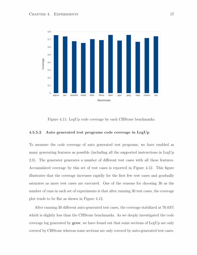
Chapter 4. Experiments 57
Figure 4.11: LegUp code coverage by each CHStone benchmarks.
4.5.5.2 Auto generated test programs code coverage in LegUp
To measure the code coverage of auto generated test programs, we have enabled as
many generating features as possible (including all the supported instructions in LegUp
2.0). The generator generates a number of different test cases with all these features.
Accumulated coverage by this set of test cases is reported in Figure 4.12. This figure
illustrates that the coverage increases rapidly for the first few test cases and gradually
saturates as more test cases are executed. One of the reasons for choosing 30 as the
number of runs in each set of experiments is that after running 30 test cases, the coverage
plot tends to be flat as shown in Figure 4.12.
After running 30 different auto-generated test cases, the coverage stabilized at 76.03%
which is slightly less than the CHStone benchmarks. As we deeply investigated the code
coverage log generated by gcov, we have found out that some sections of LegUp are only
covered by CHStone whereas some sections are only covered by auto-generated test cases.
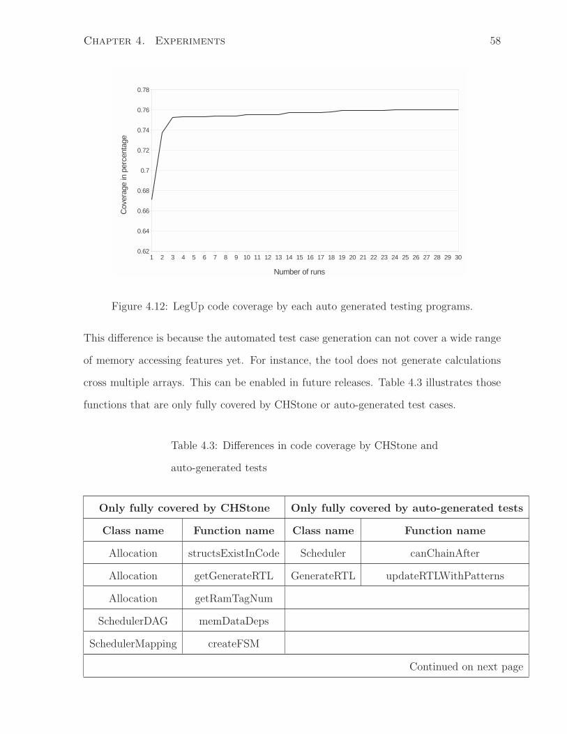
Chapter 4. Experiments 58
Figure 4.12: LegUp code coverage by each auto generated testing programs.
This difference is because the automated test case generation can not cover a wide range
of memory accessing features yet. For instance, the tool does not generate calculations
cross multiple arrays. This can be enabled in future releases. Table 4.3 illustrates those
functions that are only fully covered by CHStone or auto-generated test cases.
Table 4.3: Differences in code coverage by CHStone and
auto-generated tests
Only fully covered by CHStone Only fully covered by auto-generated tests
Class name Function name Class name Function name
Allocation structsExistInCode Scheduler canChainAfter
Allocation getGenerateRTL GenerateRTL updateRTLWithPatterns
Allocation getRamTagNum
SchedulerDAG memDataDeps
SchedulerMapping createFSM
Continued on next page
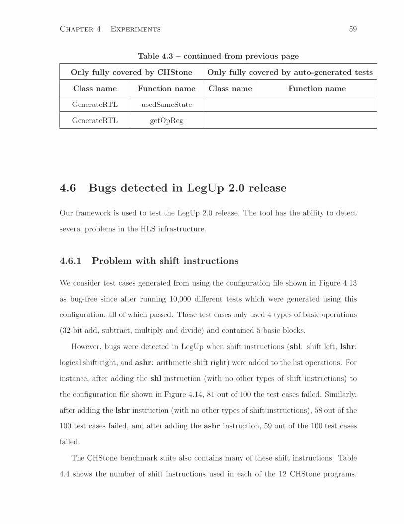
Chapter 4. Experiments 59
Table 4.3 – continued from previous page
Only fully covered by CHStone Only fully covered by auto-generated tests
Class name Function name Class name Function name
GenerateRTL usedSameState
GenerateRTL getOpReg
4.6 Bugs detected in LegUp 2.0 release
Our framework is used to test the LegUp 2.0 release. The tool has the ability to detect
several problems in the HLS infrastructure.
4.6.1 Problem with shift instructions
We consider test cases generated from using the configuration file shown in Figure 4.13
as bug-free since after running 10,000 different tests which were generated using this
configuration, all of which passed. These test cases only used 4 types of basic operations
(32-bit add, subtract, multiply and divide) and contained 5 basic blocks.
However, bugs were detected in LegUp when shift instructions (shl: shift left, lshr:
logical shift right, and ashr: arithmetic shift right) were added to the list operations. For
instance, after adding the shl instruction (with no other types of shift instructions) to
the configuration file shown in Figure 4.14, 81 out of 100 the test cases failed. Similarly,
after adding the lshr instruction (with no other types of shift instructions), 58 out of the
100 test cases failed, and after adding the ashr instruction, 59 out of the 100 test cases
failed.
The CHStone benchmark suite also contains many of these shift instructions. Table
4.4 shows the number of shift instructions used in each of the 12 CHStone programs.
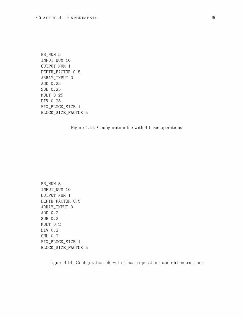
Chapter 4. Experiments 60
BB_NUM 5
INPUT_NUM 10
OUTPUT_NUM 1
DEPTH_FACTOR 0.5
ARRAY_INPUT 0
ADD 0.25
SUB 0.25
MULT 0.25
DIV 0.25
FIX_BLOCK_SIZE 1
BLOCK_SIZE_FACTOR 5
Figure 4.13: Configuration file with 4 basic operations
BB_NUM 5
INPUT_NUM 10
OUTPUT_NUM 1
DEPTH_FACTOR 0.5
ARRAY_INPUT 0
ADD 0.2
SUB 0.2
MULT 0.2
DIV 0.2
SHL 0.2
FIX_BLOCK_SIZE 1
BLOCK_SIZE_FACTOR 5
Figure 4.14: Configuration file with 4 basic operations and shl instructions
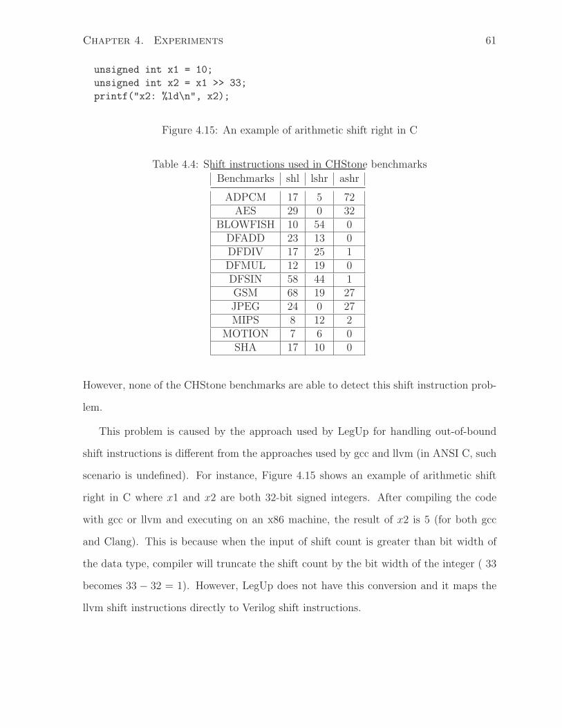
Chapter 4. Experiments 61
unsigned int x1 = 10;
unsigned int x2 = x1 >> 33;
printf("x2: %ld\n", x2);
Figure 4.15: An example of arithmetic shift right in C
Table 4.4: Shift instructions used in CHStone benchmarks
Benchmarks shl lshr ashr
ADPCM 17 5 72AES 29 0 32
BLOWFISH 10 54 0DFADD 23 13 0DFDIV 17 25 1DFMUL 12 19 0DFSIN 58 44 1GSM 68 19 27JPEG 24 0 27MIPS 8 12 2
MOTION 7 6 0SHA 17 10 0
However, none of the CHStone benchmarks are able to detect this shift instruction prob-
lem.
This problem is caused by the approach used by LegUp for handling out-of-bound
shift instructions is different from the approaches used by gcc and llvm (in ANSI C, such
scenario is undefined). For instance, Figure 4.15 shows an example of arithmetic shift
right in C where x1 and x2 are both 32-bit signed integers. After compiling the code
with gcc or llvm and executing on an x86 machine, the result of x2 is 5 (for both gcc
and Clang). This is because when the input of shift count is greater than bit width of
the data type, compiler will truncate the shift count by the bit width of the integer ( 33
becomes 33 − 32 = 1). However, LegUp does not have this conversion and it maps the
llvm shift instructions directly to Verilog shift instructions.
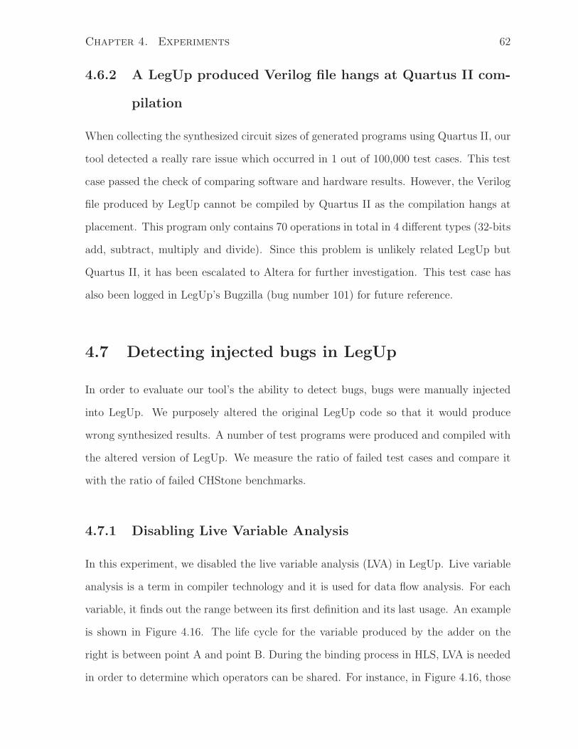
Chapter 4. Experiments 62
4.6.2 A LegUp produced Verilog file hangs at Quartus II com-
pilation
When collecting the synthesized circuit sizes of generated programs using Quartus II, our
tool detected a really rare issue which occurred in 1 out of 100,000 test cases. This test
case passed the check of comparing software and hardware results. However, the Verilog
file produced by LegUp cannot be compiled by Quartus II as the compilation hangs at
placement. This program only contains 70 operations in total in 4 different types (32-bits
add, subtract, multiply and divide). Since this problem is unlikely related LegUp but
Quartus II, it has been escalated to Altera for further investigation. This test case has
also been logged in LegUp’s Bugzilla (bug number 101) for future reference.
4.7 Detecting injected bugs in LegUp
In order to evaluate our tool’s the ability to detect bugs, bugs were manually injected
into LegUp. We purposely altered the original LegUp code so that it would produce
wrong synthesized results. A number of test programs were produced and compiled with
the altered version of LegUp. We measure the ratio of failed test cases and compare it
with the ratio of failed CHStone benchmarks.
4.7.1 Disabling Live Variable Analysis
In this experiment, we disabled the live variable analysis (LVA) in LegUp. Live variable
analysis is a term in compiler technology and it is used for data flow analysis. For each
variable, it finds out the range between its first definition and its last usage. An example
is shown in Figure 4.16. The life cycle for the variable produced by the adder on the
right is between point A and point B. During the binding process in HLS, LVA is needed
in order to determine which operators can be shared. For instance, in Figure 4.16, those
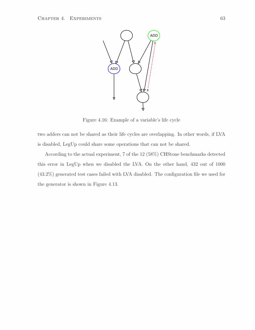
Chapter 4. Experiments 63
Figure 4.16: Example of a variable’s life cycle
two adders can not be shared as their life cycles are overlapping. In other words, if LVA
is disabled, LegUp could share some operations that can not be shared.
According to the actual experiment, 7 of the 12 (58%) CHStone benchmarks detected
this error in LegUp when we disabled the LVA. On the other hand, 432 out of 1000
(43.2%) generated test cases failed with LVA disabled. The configuration file we used for
the generator is shown in Figure 4.13.
Chapter 5
Conclusion
5.1 Summary
High-level synthesis reduces the time-to-market and lowers the design complexity of hard-
ware development. It allows a developer with less hardware skills to design hardware
using a software programing language such as C/C++/SystemC rather than a hardware
description language such as Verilog/VHDL. In a software environment, there are many
mature debugging tools which can be used for verifying and validating software programs.
However, there are a lack of tools which can be used for verifying HLS tools.
Although there exist several techniques for verifying HLS tools, those techniques have
weaknesses when compared to software debugging tools. For instance, formal methods be-
come impractical when programs get larger. Assertion-based techniques require inserting
additional code to software designs as well as hardware knowledge from the developers.
Furthermore, manually developed test suites do not have any standardized criteria to
determine the comprehensiveness of their test programs.
This work proposed an automated test case generation framework that can be used
as a complement to other existing debugging techniques for HLS tools. It can generate a
vast number of synthesizable software programs based on user specifications. These test
64
Chapter 5. Conclusion 65
cases can be simulated to verify the correctness of HLS tools.
5.2 Future work
The research in this thesis enables automated test case generation using LLVM IR for ver-
ifying, debugging and analyzing high-level synthesis tools. It provides additional options
for HLS developers to validate their designs. A number of future potential directions
are proposed to extend this framework in order to extend the features supported by the
generator as well as to add more intelligence to the graph generation.
5.2.1 Input vector range analysis for test programs
Currently, the test vectors generated for the test programs are created randomly without
much constraints. This can make the execution of test programs unrealistic. For instance,
overflow and underflow (e.g. floating point numbers) can occur often during calculations.
One of the potential solutions to this problem is to use the range analysis described
in [24]. The author of [24] proposed an algorithm modeled after a constraint-based
framework from [25], wherein the program is analyzed to obey a set of constraints defining
the range of each variable. In the case of our work, for instance, users may want to
produce test cases with non-zero results. This range analysis can help the generator
to figure out a preferable input vector range and therefore increase the quality of test
programs.
5.2.2 Back tracing the error points
Currently, the debugging framework only tells the user whether a test case has passed
or not by comparing the final results. However, it does not have the ability to determine
which section of the code caused the problem.
This can be improved by creating accurate mappings between each step of software
Chapter 5. Conclusion 66
and hardware execution so that the user can verify the results after the execution of each
operation.
Another potential improvement is to create a GDB-like debugging framework for
high-level synthesis tools. Similar to [15], it can provide a graphic representation of
source-level mappings between software code and synthesized circuits with break points
to step through the code for investigation.
5.2.3 Customizable pattern injection
Generating patterns randomly preserves more randomness in test cases to help developers
verify the correctness. However, it is worth having a tool that lets the user specify what
patterns should appear in the network, which gives the users the ability to analyze which
kind of network structures are worth sharing in certain FPGA devices. Currently, the
user can manually code pre-defined patterns inside the generator framework. In the
future, the tool should provide a dot-like language [1] that describes network structures
using plain text.
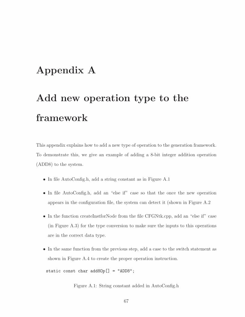
Appendix A
Add new operation type to the
framework
This appendix explains how to add a new type of operation to the generation framework.
To demonstrate this, we give an example of adding a 8-bit integer addition operation
(ADD8) to the system.
• In file AutoConfig.h, add a string constant as in Figure A.1
• In file AutoConfig.h, add an “else if” case so that the once the new operation
appears in the configuration file, the system can detect it (shown in Figure A.2
• In the function createInstforNode from the file CFGNtk.cpp, add an “else if” case
(in Figure A.3) for the type conversion to make sure the inputs to this operations
are in the correct data type.
• In the same function from the previous step, add a case to the switch statement as
shown in Figure A.4 to create the proper operation instruction.
static const char add8Op[] = "ADD8";
Figure A.1: String constant added in AutoConfig.h
67
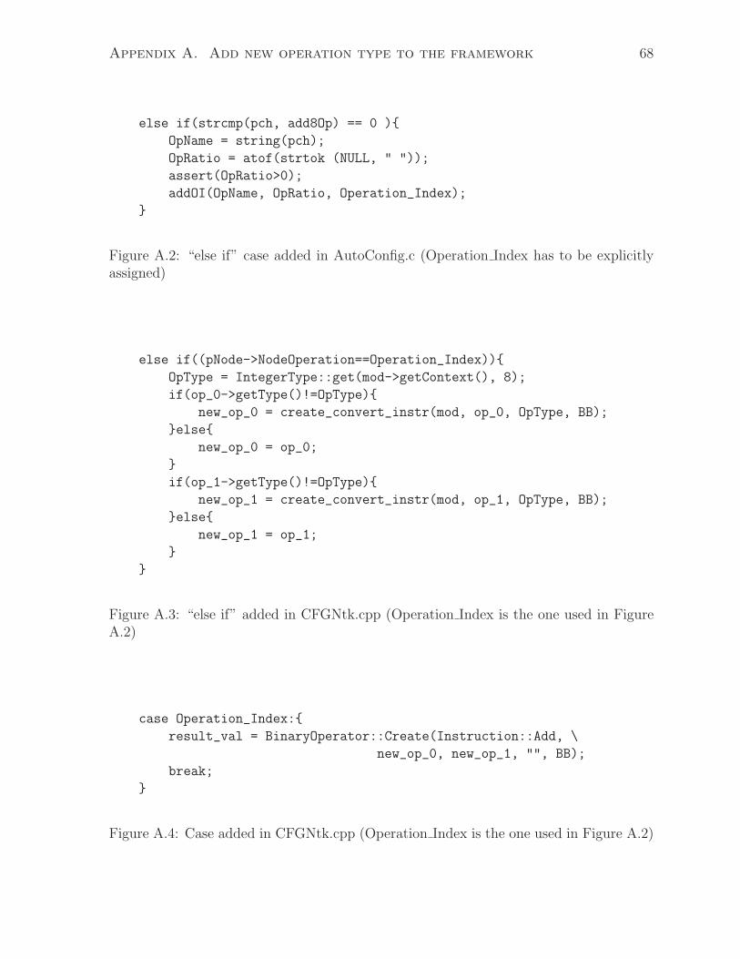
Appendix A. Add new operation type to the framework 68
else if(strcmp(pch, add8Op) == 0 ){
OpName = string(pch);
OpRatio = atof(strtok (NULL, " "));
assert(OpRatio>0);
addOI(OpName, OpRatio, Operation_Index);
}
Figure A.2: “else if” case added in AutoConfig.c (Operation Index has to be explicitlyassigned)
else if((pNode->NodeOperation==Operation_Index)){
OpType = IntegerType::get(mod->getContext(), 8);
if(op_0->getType()!=OpType){
new_op_0 = create_convert_instr(mod, op_0, OpType, BB);
}else{
new_op_0 = op_0;
}
if(op_1->getType()!=OpType){
new_op_1 = create_convert_instr(mod, op_1, OpType, BB);
}else{
new_op_1 = op_1;
}
}
Figure A.3: “else if” added in CFGNtk.cpp (Operation Index is the one used in FigureA.2)
case Operation_Index:{
result_val = BinaryOperator::Create(Instruction::Add, \
new_op_0, new_op_1, "", BB);
break;
}
Figure A.4: Case added in CFGNtk.cpp (Operation Index is the one used in Figure A.2)
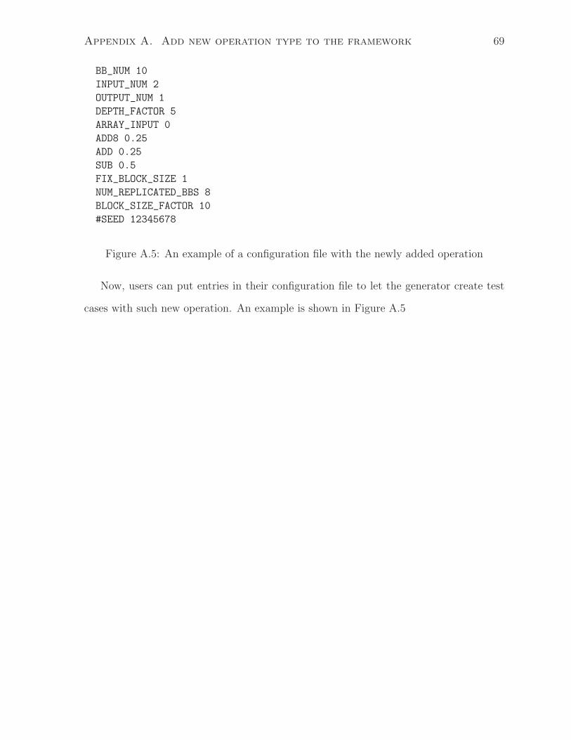
Appendix A. Add new operation type to the framework 69
BB_NUM 10
INPUT_NUM 2
OUTPUT_NUM 1
DEPTH_FACTOR 5
ARRAY_INPUT 0
ADD8 0.25
ADD 0.25
SUB 0.5
FIX_BLOCK_SIZE 1
NUM_REPLICATED_BBS 8
BLOCK_SIZE_FACTOR 10
#SEED 12345678
Figure A.5: An example of a configuration file with the newly added operation
Now, users can put entries in their configuration file to let the generator create test
cases with such new operation. An example is shown in Figure A.5
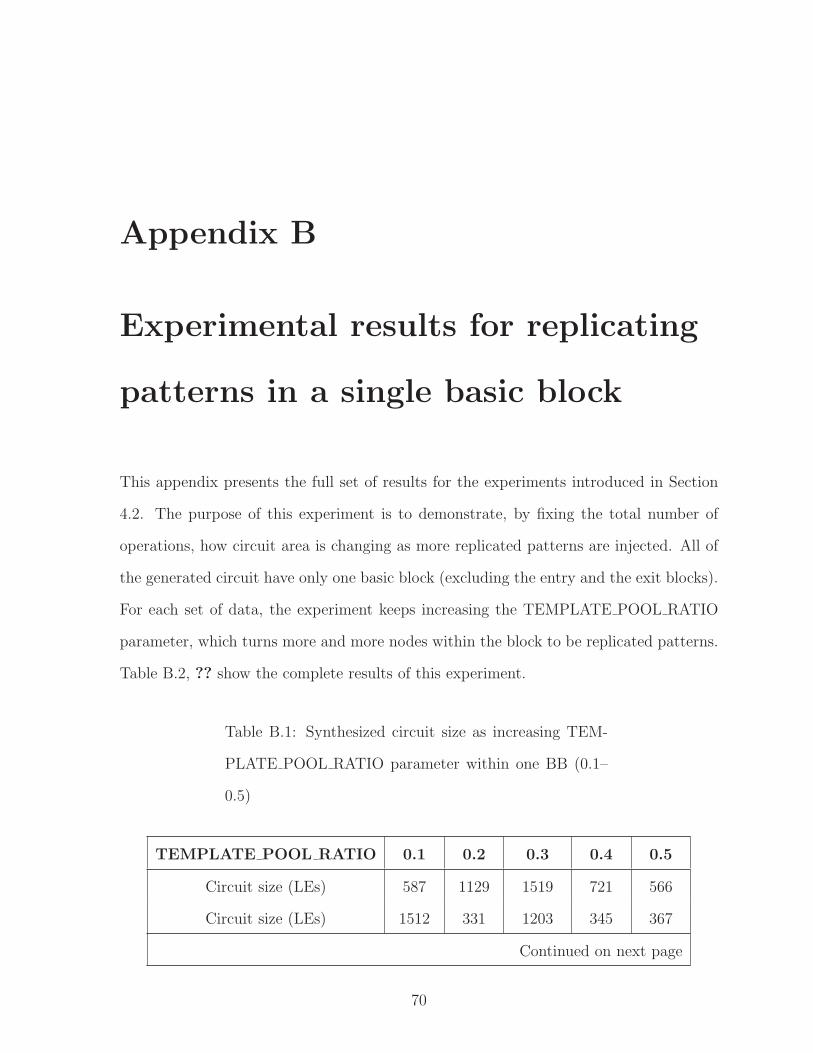
Appendix B
Experimental results for replicating
patterns in a single basic block
This appendix presents the full set of results for the experiments introduced in Section
4.2. The purpose of this experiment is to demonstrate, by fixing the total number of
operations, how circuit area is changing as more replicated patterns are injected. All of
the generated circuit have only one basic block (excluding the entry and the exit blocks).
For each set of data, the experiment keeps increasing the TEMPLATE POOL RATIO
parameter, which turns more and more nodes within the block to be replicated patterns.
Table B.2, ?? show the complete results of this experiment.
Table B.1: Synthesized circuit size as increasing TEM-
PLATE POOL RATIO parameter within one BB (0.1–
0.5)
TEMPLATE POOL RATIO 0.1 0.2 0.3 0.4 0.5
Circuit size (LEs) 587 1129 1519 721 566
Circuit size (LEs) 1512 331 1203 345 367
Continued on next page
70
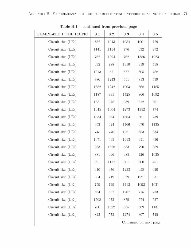
Appendix B. Experimental results for replicating patterns in a single basic block71
Table B.1 – continued from previous page
TEMPLATE POOL RATIO 0.1 0.2 0.3 0.4 0.5
Circuit size (LEs) 882 1043 1084 1001 729
Circuit size (LEs) 1141 1154 776 632 972
Circuit size (LEs) 762 1294 762 1386 1023
Circuit size (LEs) 632 788 1310 919 458
Circuit size (LEs) 1013 57 677 605 788
Circuit size (LEs) 886 1243 551 813 539
Circuit size (LEs) 1682 1242 1903 668 1185
Circuit size (LEs) 1187 831 1725 866 1092
Circuit size (LEs) 1551 978 939 512 561
Circuit size (LEs) 1045 1004 1273 1352 774
Circuit size (LEs) 1534 634 1363 861 739
Circuit size (LEs) 653 624 1466 670 1135
Circuit size (LEs) 745 740 1221 683 934
Circuit size (LEs) 1071 695 1913 951 336
Circuit size (LEs) 963 1628 533 790 889
Circuit size (LEs) 881 996 985 426 1035
Circuit size (LEs) 891 1177 501 500 451
Circuit size (LEs) 910 976 1233 658 620
Circuit size (LEs) 584 719 679 1221 931
Circuit size (LEs) 759 749 1412 1092 1031
Circuit size (LEs) 664 507 1207 715 733
Circuit size (LEs) 1508 673 879 574 537
Circuit size (LEs) 780 1322 835 669 1131
Circuit size (LEs) 822 573 1274 307 745
Continued on next page
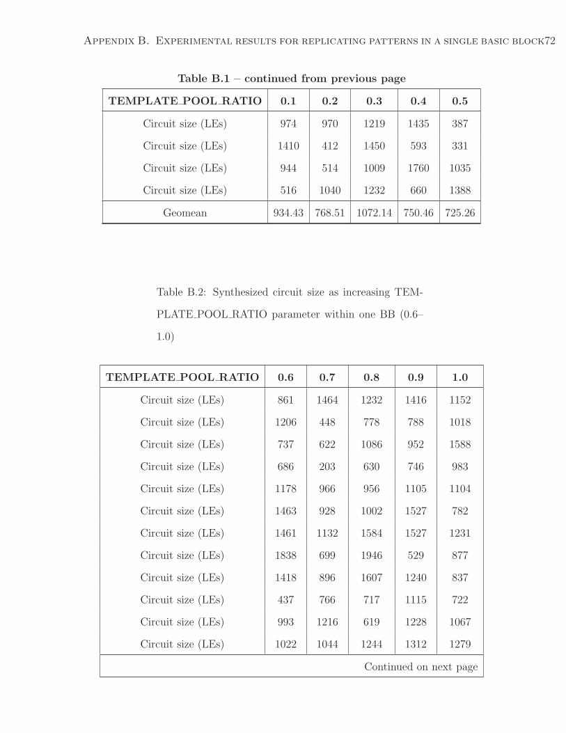
Appendix B. Experimental results for replicating patterns in a single basic block72
Table B.1 – continued from previous page
TEMPLATE POOL RATIO 0.1 0.2 0.3 0.4 0.5
Circuit size (LEs) 974 970 1219 1435 387
Circuit size (LEs) 1410 412 1450 593 331
Circuit size (LEs) 944 514 1009 1760 1035
Circuit size (LEs) 516 1040 1232 660 1388
Geomean 934.43 768.51 1072.14 750.46 725.26
Table B.2: Synthesized circuit size as increasing TEM-
PLATE POOL RATIO parameter within one BB (0.6–
1.0)
TEMPLATE POOL RATIO 0.6 0.7 0.8 0.9 1.0
Circuit size (LEs) 861 1464 1232 1416 1152
Circuit size (LEs) 1206 448 778 788 1018
Circuit size (LEs) 737 622 1086 952 1588
Circuit size (LEs) 686 203 630 746 983
Circuit size (LEs) 1178 966 956 1105 1104
Circuit size (LEs) 1463 928 1002 1527 782
Circuit size (LEs) 1461 1132 1584 1527 1231
Circuit size (LEs) 1838 699 1946 529 877
Circuit size (LEs) 1418 896 1607 1240 837
Circuit size (LEs) 437 766 717 1115 722
Circuit size (LEs) 993 1216 619 1228 1067
Circuit size (LEs) 1022 1044 1244 1312 1279
Continued on next page
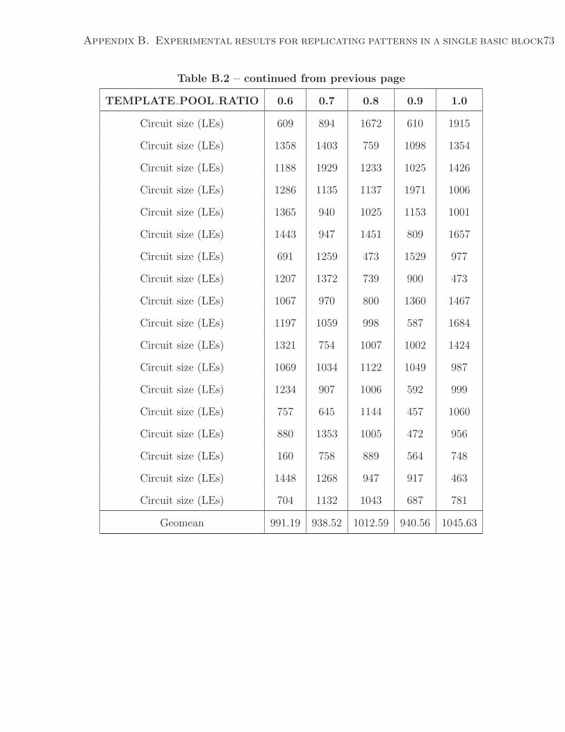
Appendix B. Experimental results for replicating patterns in a single basic block73
Table B.2 – continued from previous page
TEMPLATE POOL RATIO 0.6 0.7 0.8 0.9 1.0
Circuit size (LEs) 609 894 1672 610 1915
Circuit size (LEs) 1358 1403 759 1098 1354
Circuit size (LEs) 1188 1929 1233 1025 1426
Circuit size (LEs) 1286 1135 1137 1971 1006
Circuit size (LEs) 1365 940 1025 1153 1001
Circuit size (LEs) 1443 947 1451 809 1657
Circuit size (LEs) 691 1259 473 1529 977
Circuit size (LEs) 1207 1372 739 900 473
Circuit size (LEs) 1067 970 800 1360 1467
Circuit size (LEs) 1197 1059 998 587 1684
Circuit size (LEs) 1321 754 1007 1002 1424
Circuit size (LEs) 1069 1034 1122 1049 987
Circuit size (LEs) 1234 907 1006 592 999
Circuit size (LEs) 757 645 1144 457 1060
Circuit size (LEs) 880 1353 1005 472 956
Circuit size (LEs) 160 758 889 564 748
Circuit size (LEs) 1448 1268 947 917 463
Circuit size (LEs) 704 1132 1043 687 781
Geomean 991.19 938.52 1012.59 940.56 1045.63
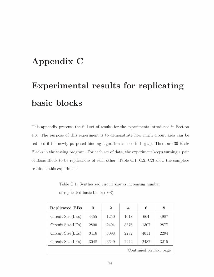
Appendix C
Experimental results for replicating
basic blocks
This appendix presents the full set of results for the experiments introduced in Section
4.3. The purpose of this experiment is to demonstrate how much circuit area can be
reduced if the newly purposed binding algorithm is used in LegUp. There are 30 Basic
Blocks in the testing program. For each set of data, the experiment keeps turning a pair
of Basic Block to be replications of each other. Table C.1, C.2, C.3 show the complete
results of this experiment.
Table C.1: Synthesized circuit size as increasing number
of replicated basic blocks(0–8)
Replicated BBs 0 2 4 6 8
Circuit Size(LEs) 4455 1250 1618 664 4987
Circuit Size(LEs) 2800 2494 3576 1307 2877
Circuit Size(LEs) 3416 3098 2282 4011 2294
Circuit Size(LEs) 3048 3649 2242 2482 3215
Continued on next page
74
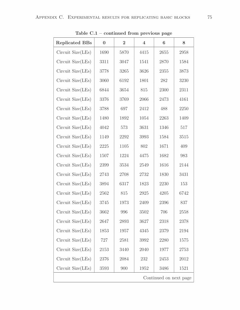
Appendix C. Experimental results for replicating basic blocks 75
Table C.1 – continued from previous page
Replicated BBs 0 2 4 6 8
Circuit Size(LEs) 1690 5870 4415 2655 2958
Circuit Size(LEs) 3311 3047 1541 2870 1584
Circuit Size(LEs) 3778 3265 3626 2355 3873
Circuit Size(LEs) 3060 6192 1801 282 3230
Circuit Size(LEs) 6844 3654 815 2300 2311
Circuit Size(LEs) 3376 3769 2066 2473 4161
Circuit Size(LEs) 3788 697 2412 488 2250
Circuit Size(LEs) 1480 1892 1054 2263 1409
Circuit Size(LEs) 4042 573 3631 1346 517
Circuit Size(LEs) 1149 2292 3993 1584 3515
Circuit Size(LEs) 2225 1105 802 1671 409
Circuit Size(LEs) 1507 1224 4475 1682 983
Circuit Size(LEs) 2399 3534 2549 1616 2144
Circuit Size(LEs) 2743 2708 2732 1830 3431
Circuit Size(LEs) 3894 6317 1823 2230 153
Circuit Size(LEs) 2562 815 2925 4205 6742
Circuit Size(LEs) 3745 1973 2409 2396 837
Circuit Size(LEs) 3662 996 3502 706 2558
Circuit Size(LEs) 2647 2893 3627 2318 2378
Circuit Size(LEs) 1853 1957 4345 2379 2194
Circuit Size(LEs) 727 2581 3992 2280 1575
Circuit Size(LEs) 2153 3440 2040 1977 2753
Circuit Size(LEs) 2376 2084 232 2453 2012
Circuit Size(LEs) 3593 900 1952 3486 1521
Continued on next page
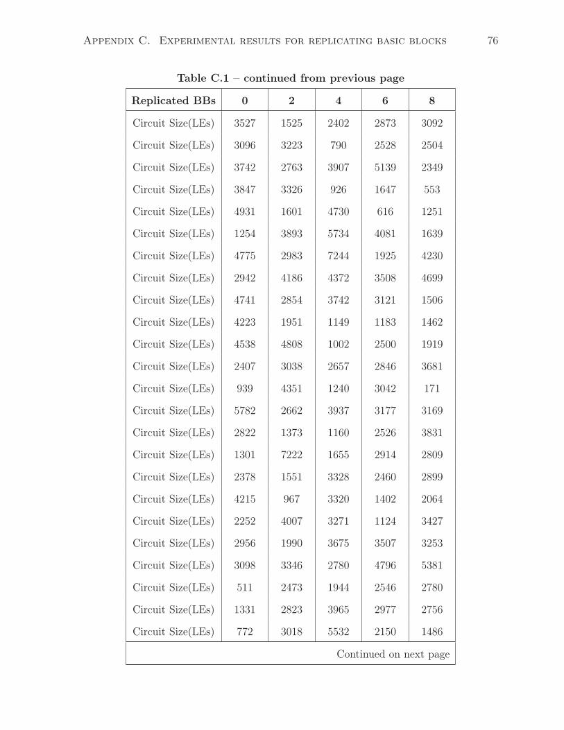
Appendix C. Experimental results for replicating basic blocks 76
Table C.1 – continued from previous page
Replicated BBs 0 2 4 6 8
Circuit Size(LEs) 3527 1525 2402 2873 3092
Circuit Size(LEs) 3096 3223 790 2528 2504
Circuit Size(LEs) 3742 2763 3907 5139 2349
Circuit Size(LEs) 3847 3326 926 1647 553
Circuit Size(LEs) 4931 1601 4730 616 1251
Circuit Size(LEs) 1254 3893 5734 4081 1639
Circuit Size(LEs) 4775 2983 7244 1925 4230
Circuit Size(LEs) 2942 4186 4372 3508 4699
Circuit Size(LEs) 4741 2854 3742 3121 1506
Circuit Size(LEs) 4223 1951 1149 1183 1462
Circuit Size(LEs) 4538 4808 1002 2500 1919
Circuit Size(LEs) 2407 3038 2657 2846 3681
Circuit Size(LEs) 939 4351 1240 3042 171
Circuit Size(LEs) 5782 2662 3937 3177 3169
Circuit Size(LEs) 2822 1373 1160 2526 3831
Circuit Size(LEs) 1301 7222 1655 2914 2809
Circuit Size(LEs) 2378 1551 3328 2460 2899
Circuit Size(LEs) 4215 967 3320 1402 2064
Circuit Size(LEs) 2252 4007 3271 1124 3427
Circuit Size(LEs) 2956 1990 3675 3507 3253
Circuit Size(LEs) 3098 3346 2780 4796 5381
Circuit Size(LEs) 511 2473 1944 2546 2780
Circuit Size(LEs) 1331 2823 3965 2977 2756
Circuit Size(LEs) 772 3018 5532 2150 1486
Continued on next page

Appendix C. Experimental results for replicating basic blocks 77
Table C.1 – continued from previous page
Replicated BBs 0 2 4 6 8
Circuit Size(LEs) 3195 4607 830 3091 3798
Circuit Size(LEs) 1553 2315 4830 2826 2303
Circuit Size(LEs) 1803 4493 2196 2054 5095
Circuit Size(LEs) 3988 2618 390 4950 2831
Circuit Size(LEs) 2751 4781 480 6692 3129
Circuit Size(LEs) 5273 2477 3210 2637 1631
Circuit Size(LEs) 4000 6938 468 6191 3165
Circuit Size(LEs) 1547 4006 3563 1362 2978
Circuit Size(LEs) 2375 4160 3026 2724 5777
Circuit Size(LEs) 3119 2835 3604 2334 2962
Circuit Size(LEs) 2275 1168 1829 1687 2031
Circuit Size(LEs) 5761 2748 2201 2471 3329
Circuit Size(LEs) 2554 2751 1376 2624 2709
Circuit Size(LEs) 3773 1911 1965 1065 2140
Circuit Size(LEs) 3061 3619 778 1231 1165
Circuit Size(LEs) 2194 5736 534 2531 4540
Circuit Size(LEs) 3292 5933 3810 3037 1919
Circuit Size(LEs) 4104 2332 1618 2251 2559
Circuit Size(LEs) 3501 5503 2113 3408 2273
Circuit Size(LEs) 2557 3375 3593 4678 1206
Circuit Size(LEs) 1869 2480 3071 2337 4260
Circuit Size(LEs) 3847 1450 1220 1144 680
Circuit Size(LEs) 994 641 5561 2291 4167
Circuit Size(LEs) 3232 1722 982 945 3961
Continued on next page
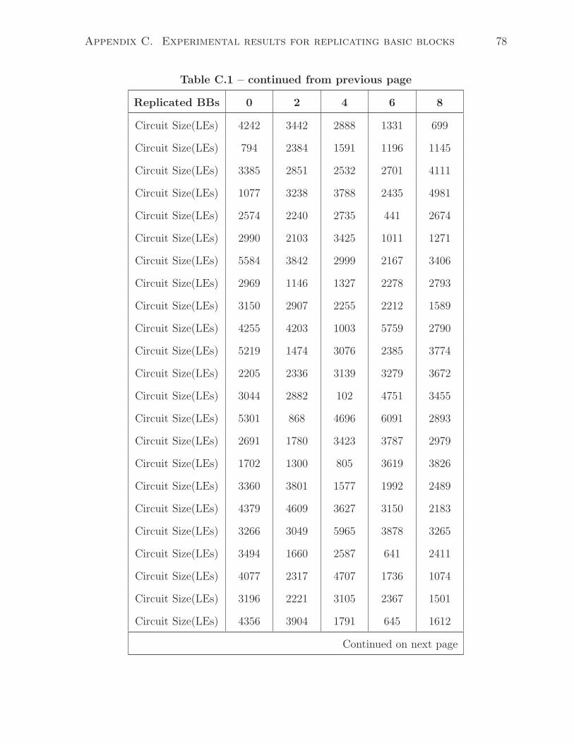
Appendix C. Experimental results for replicating basic blocks 78
Table C.1 – continued from previous page
Replicated BBs 0 2 4 6 8
Circuit Size(LEs) 4242 3442 2888 1331 699
Circuit Size(LEs) 794 2384 1591 1196 1145
Circuit Size(LEs) 3385 2851 2532 2701 4111
Circuit Size(LEs) 1077 3238 3788 2435 4981
Circuit Size(LEs) 2574 2240 2735 441 2674
Circuit Size(LEs) 2990 2103 3425 1011 1271
Circuit Size(LEs) 5584 3842 2999 2167 3406
Circuit Size(LEs) 2969 1146 1327 2278 2793
Circuit Size(LEs) 3150 2907 2255 2212 1589
Circuit Size(LEs) 4255 4203 1003 5759 2790
Circuit Size(LEs) 5219 1474 3076 2385 3774
Circuit Size(LEs) 2205 2336 3139 3279 3672
Circuit Size(LEs) 3044 2882 102 4751 3455
Circuit Size(LEs) 5301 868 4696 6091 2893
Circuit Size(LEs) 2691 1780 3423 3787 2979
Circuit Size(LEs) 1702 1300 805 3619 3826
Circuit Size(LEs) 3360 3801 1577 1992 2489
Circuit Size(LEs) 4379 4609 3627 3150 2183
Circuit Size(LEs) 3266 3049 5965 3878 3265
Circuit Size(LEs) 3494 1660 2587 641 2411
Circuit Size(LEs) 4077 2317 4707 1736 1074
Circuit Size(LEs) 3196 2221 3105 2367 1501
Circuit Size(LEs) 4356 3904 1791 645 1612
Continued on next page
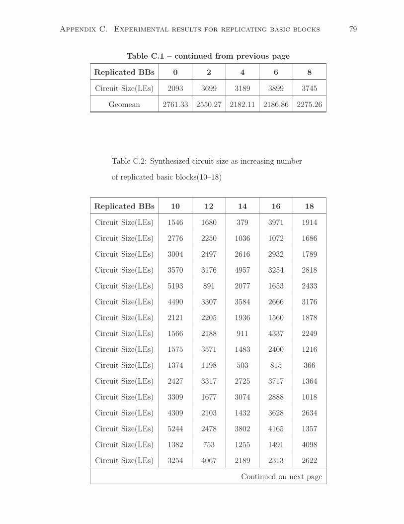
Appendix C. Experimental results for replicating basic blocks 79
Table C.1 – continued from previous page
Replicated BBs 0 2 4 6 8
Circuit Size(LEs) 2093 3699 3189 3899 3745
Geomean 2761.33 2550.27 2182.11 2186.86 2275.26
Table C.2: Synthesized circuit size as increasing number
of replicated basic blocks(10–18)
Replicated BBs 10 12 14 16 18
Circuit Size(LEs) 1546 1680 379 3971 1914
Circuit Size(LEs) 2776 2250 1036 1072 1686
Circuit Size(LEs) 3004 2497 2616 2932 1789
Circuit Size(LEs) 3570 3176 4957 3254 2818
Circuit Size(LEs) 5193 891 2077 1653 2433
Circuit Size(LEs) 4490 3307 3584 2666 3176
Circuit Size(LEs) 2121 2205 1936 1560 1878
Circuit Size(LEs) 1566 2188 911 4337 2249
Circuit Size(LEs) 1575 3571 1483 2400 1216
Circuit Size(LEs) 1374 1198 503 815 366
Circuit Size(LEs) 2427 3317 2725 3717 1364
Circuit Size(LEs) 3309 1677 3074 2888 1018
Circuit Size(LEs) 4309 2103 1432 3628 2634
Circuit Size(LEs) 5244 2478 3802 4165 1357
Circuit Size(LEs) 1382 753 1255 1491 4098
Circuit Size(LEs) 3254 4067 2189 2313 2622
Continued on next page
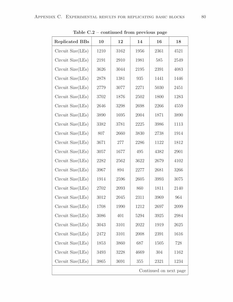
Appendix C. Experimental results for replicating basic blocks 80
Table C.2 – continued from previous page
Replicated BBs 10 12 14 16 18
Circuit Size(LEs) 1210 3162 1956 2361 4521
Circuit Size(LEs) 2191 2910 1981 585 2549
Circuit Size(LEs) 3626 3044 2195 2391 4083
Circuit Size(LEs) 2878 1381 935 1441 1446
Circuit Size(LEs) 2779 3077 2271 5030 2451
Circuit Size(LEs) 3702 1876 2502 1800 1283
Circuit Size(LEs) 2646 3298 2698 2266 4559
Circuit Size(LEs) 3890 1695 2004 1871 3890
Circuit Size(LEs) 3382 3781 2225 3986 1113
Circuit Size(LEs) 807 2660 3830 2738 1914
Circuit Size(LEs) 3671 277 2286 1122 1812
Circuit Size(LEs) 3057 1677 495 4382 2901
Circuit Size(LEs) 2282 2562 3622 2679 4102
Circuit Size(LEs) 3967 894 2277 2681 3266
Circuit Size(LEs) 1914 2596 2605 3993 3075
Circuit Size(LEs) 2702 2093 860 1811 2140
Circuit Size(LEs) 3012 2045 2311 3969 964
Circuit Size(LEs) 1708 1990 1212 2697 2099
Circuit Size(LEs) 3086 401 5294 3925 2984
Circuit Size(LEs) 3043 3101 2022 1919 2625
Circuit Size(LEs) 2472 3101 2008 2391 1616
Circuit Size(LEs) 1853 3860 687 1505 728
Circuit Size(LEs) 3493 3228 4669 304 1162
Circuit Size(LEs) 3865 3691 355 2321 1234
Continued on next page
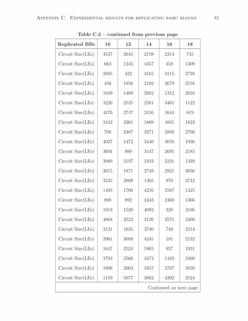
Appendix C. Experimental results for replicating basic blocks 81
Table C.2 – continued from previous page
Replicated BBs 10 12 14 16 18
Circuit Size(LEs) 4537 2645 2159 2314 745
Circuit Size(LEs) 663 1245 4357 358 1309
Circuit Size(LEs) 2685 422 3165 3115 2738
Circuit Size(LEs) 456 1856 2192 2679 2158
Circuit Size(LEs) 1049 1469 2602 1312 2616
Circuit Size(LEs) 3226 2525 2581 3401 1122
Circuit Size(LEs) 4470 2747 2416 1644 819
Circuit Size(LEs) 2442 3361 1869 4831 1822
Circuit Size(LEs) 708 2407 3271 2888 2700
Circuit Size(LEs) 4027 1472 3440 3076 1936
Circuit Size(LEs) 3694 989 3147 2695 2185
Circuit Size(LEs) 3089 2197 2433 2191 1339
Circuit Size(LEs) 3015 1871 2749 2921 3056
Circuit Size(LEs) 3535 2808 1365 970 3742
Circuit Size(LEs) 1495 1700 4216 2587 1425
Circuit Size(LEs) 888 892 2443 2368 1366
Circuit Size(LEs) 1013 1538 4092 320 3186
Circuit Size(LEs) 4868 3522 3126 3575 2400
Circuit Size(LEs) 3121 1635 3740 749 2214
Circuit Size(LEs) 2061 3089 4245 181 2132
Circuit Size(LEs) 1647 2524 5965 957 1931
Circuit Size(LEs) 3793 2566 3473 1163 2460
Circuit Size(LEs) 1006 2663 3457 2707 5050
Circuit Size(LEs) 1159 5077 2662 4392 2524
Continued on next page
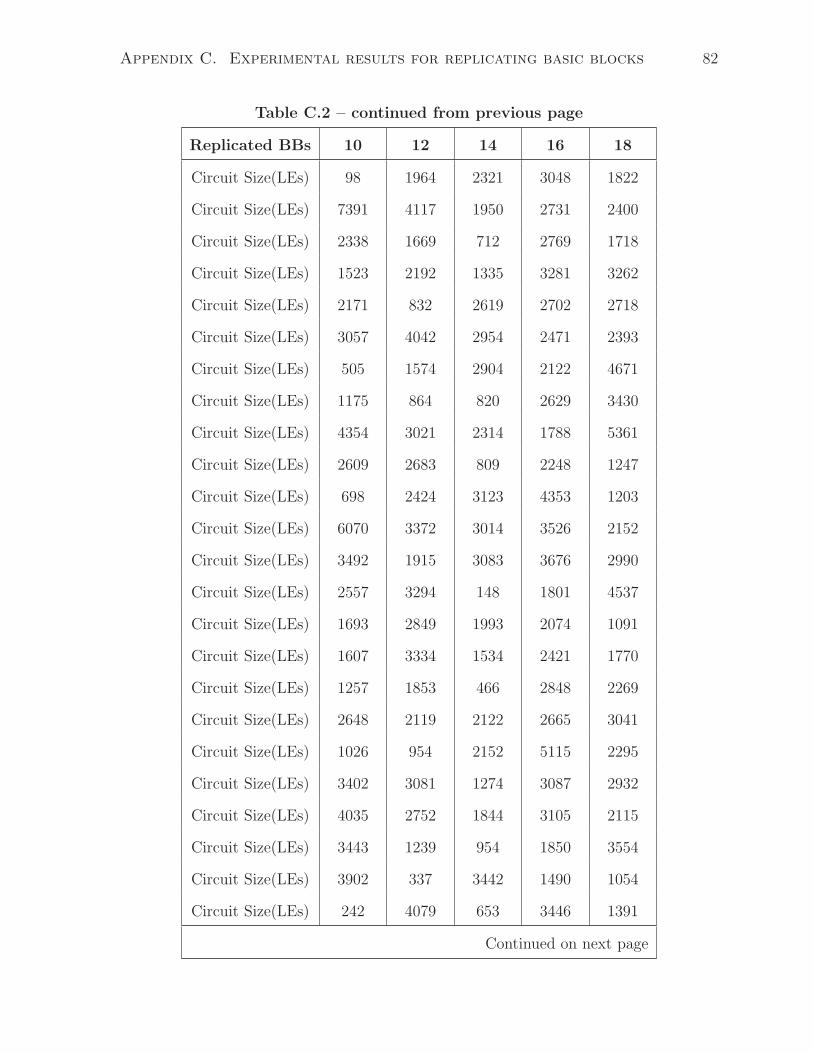
Appendix C. Experimental results for replicating basic blocks 82
Table C.2 – continued from previous page
Replicated BBs 10 12 14 16 18
Circuit Size(LEs) 98 1964 2321 3048 1822
Circuit Size(LEs) 7391 4117 1950 2731 2400
Circuit Size(LEs) 2338 1669 712 2769 1718
Circuit Size(LEs) 1523 2192 1335 3281 3262
Circuit Size(LEs) 2171 832 2619 2702 2718
Circuit Size(LEs) 3057 4042 2954 2471 2393
Circuit Size(LEs) 505 1574 2904 2122 4671
Circuit Size(LEs) 1175 864 820 2629 3430
Circuit Size(LEs) 4354 3021 2314 1788 5361
Circuit Size(LEs) 2609 2683 809 2248 1247
Circuit Size(LEs) 698 2424 3123 4353 1203
Circuit Size(LEs) 6070 3372 3014 3526 2152
Circuit Size(LEs) 3492 1915 3083 3676 2990
Circuit Size(LEs) 2557 3294 148 1801 4537
Circuit Size(LEs) 1693 2849 1993 2074 1091
Circuit Size(LEs) 1607 3334 1534 2421 1770
Circuit Size(LEs) 1257 1853 466 2848 2269
Circuit Size(LEs) 2648 2119 2122 2665 3041
Circuit Size(LEs) 1026 954 2152 5115 2295
Circuit Size(LEs) 3402 3081 1274 3087 2932
Circuit Size(LEs) 4035 2752 1844 3105 2115
Circuit Size(LEs) 3443 1239 954 1850 3554
Circuit Size(LEs) 3902 337 3442 1490 1054
Circuit Size(LEs) 242 4079 653 3446 1391
Continued on next page
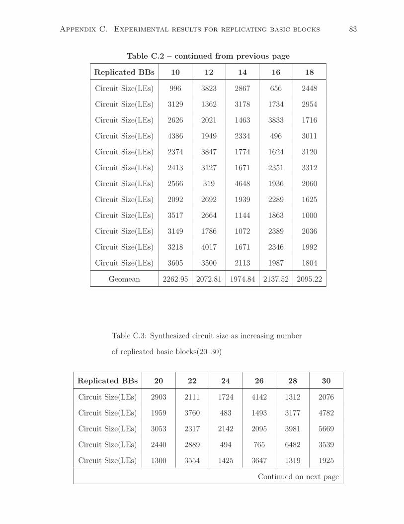
Appendix C. Experimental results for replicating basic blocks 83
Table C.2 – continued from previous page
Replicated BBs 10 12 14 16 18
Circuit Size(LEs) 996 3823 2867 656 2448
Circuit Size(LEs) 3129 1362 3178 1734 2954
Circuit Size(LEs) 2626 2021 1463 3833 1716
Circuit Size(LEs) 4386 1949 2334 496 3011
Circuit Size(LEs) 2374 3847 1774 1624 3120
Circuit Size(LEs) 2413 3127 1671 2351 3312
Circuit Size(LEs) 2566 319 4648 1936 2060
Circuit Size(LEs) 2092 2692 1939 2289 1625
Circuit Size(LEs) 3517 2664 1144 1863 1000
Circuit Size(LEs) 3149 1786 1072 2389 2036
Circuit Size(LEs) 3218 4017 1671 2346 1992
Circuit Size(LEs) 3605 3500 2113 1987 1804
Geomean 2262.95 2072.81 1974.84 2137.52 2095.22
Table C.3: Synthesized circuit size as increasing number
of replicated basic blocks(20–30)
Replicated BBs 20 22 24 26 28 30
Circuit Size(LEs) 2903 2111 1724 4142 1312 2076
Circuit Size(LEs) 1959 3760 483 1493 3177 4782
Circuit Size(LEs) 3053 2317 2142 2095 3981 5669
Circuit Size(LEs) 2440 2889 494 765 6482 3539
Circuit Size(LEs) 1300 3554 1425 3647 1319 1925
Continued on next page
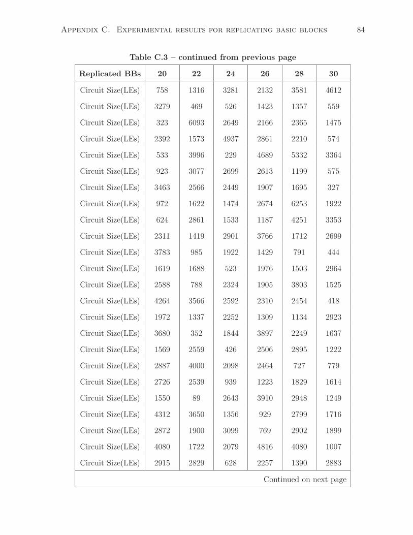
Appendix C. Experimental results for replicating basic blocks 84
Table C.3 – continued from previous page
Replicated BBs 20 22 24 26 28 30
Circuit Size(LEs) 758 1316 3281 2132 3581 4612
Circuit Size(LEs) 3279 469 526 1423 1357 559
Circuit Size(LEs) 323 6093 2649 2166 2365 1475
Circuit Size(LEs) 2392 1573 4937 2861 2210 574
Circuit Size(LEs) 533 3996 229 4689 5332 3364
Circuit Size(LEs) 923 3077 2699 2613 1199 575
Circuit Size(LEs) 3463 2566 2449 1907 1695 327
Circuit Size(LEs) 972 1622 1474 2674 6253 1922
Circuit Size(LEs) 624 2861 1533 1187 4251 3353
Circuit Size(LEs) 2311 1419 2901 3766 1712 2699
Circuit Size(LEs) 3783 985 1922 1429 791 444
Circuit Size(LEs) 1619 1688 523 1976 1503 2964
Circuit Size(LEs) 2588 788 2324 1905 3803 1525
Circuit Size(LEs) 4264 3566 2592 2310 2454 418
Circuit Size(LEs) 1972 1337 2252 1309 1134 2923
Circuit Size(LEs) 3680 352 1844 3897 2249 1637
Circuit Size(LEs) 1569 2559 426 2506 2895 1222
Circuit Size(LEs) 2887 4000 2098 2464 727 779
Circuit Size(LEs) 2726 2539 939 1223 1829 1614
Circuit Size(LEs) 1550 89 2643 3910 2948 1249
Circuit Size(LEs) 4312 3650 1356 929 2799 1716
Circuit Size(LEs) 2872 1900 3099 769 2902 1899
Circuit Size(LEs) 4080 1722 2079 4816 4080 1007
Circuit Size(LEs) 2915 2829 628 2257 1390 2883
Continued on next page
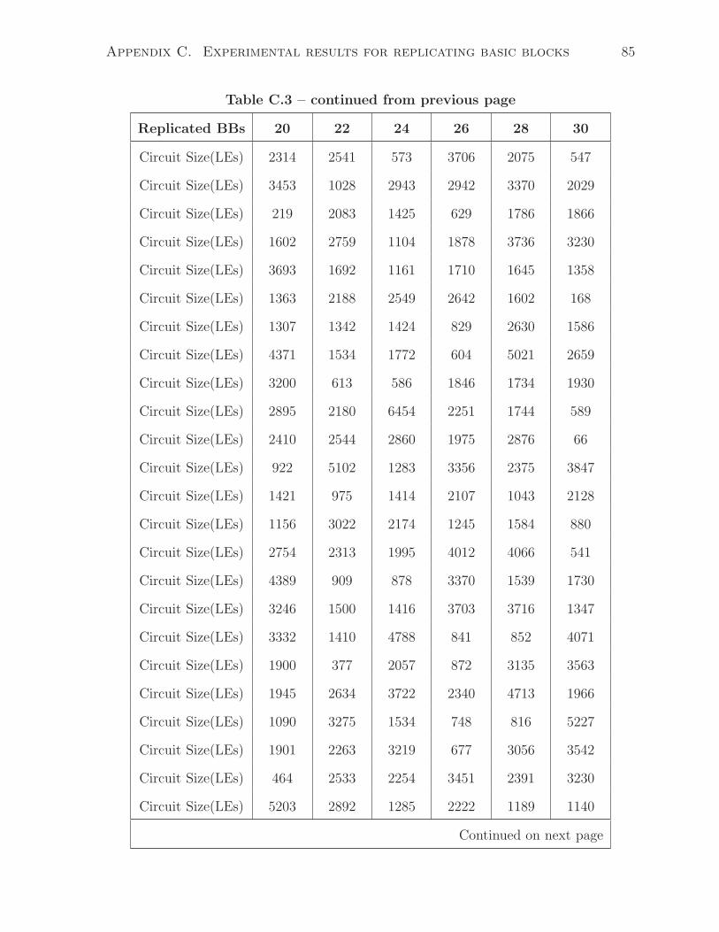
Appendix C. Experimental results for replicating basic blocks 85
Table C.3 – continued from previous page
Replicated BBs 20 22 24 26 28 30
Circuit Size(LEs) 2314 2541 573 3706 2075 547
Circuit Size(LEs) 3453 1028 2943 2942 3370 2029
Circuit Size(LEs) 219 2083 1425 629 1786 1866
Circuit Size(LEs) 1602 2759 1104 1878 3736 3230
Circuit Size(LEs) 3693 1692 1161 1710 1645 1358
Circuit Size(LEs) 1363 2188 2549 2642 1602 168
Circuit Size(LEs) 1307 1342 1424 829 2630 1586
Circuit Size(LEs) 4371 1534 1772 604 5021 2659
Circuit Size(LEs) 3200 613 586 1846 1734 1930
Circuit Size(LEs) 2895 2180 6454 2251 1744 589
Circuit Size(LEs) 2410 2544 2860 1975 2876 66
Circuit Size(LEs) 922 5102 1283 3356 2375 3847
Circuit Size(LEs) 1421 975 1414 2107 1043 2128
Circuit Size(LEs) 1156 3022 2174 1245 1584 880
Circuit Size(LEs) 2754 2313 1995 4012 4066 541
Circuit Size(LEs) 4389 909 878 3370 1539 1730
Circuit Size(LEs) 3246 1500 1416 3703 3716 1347
Circuit Size(LEs) 3332 1410 4788 841 852 4071
Circuit Size(LEs) 1900 377 2057 872 3135 3563
Circuit Size(LEs) 1945 2634 3722 2340 4713 1966
Circuit Size(LEs) 1090 3275 1534 748 816 5227
Circuit Size(LEs) 1901 2263 3219 677 3056 3542
Circuit Size(LEs) 464 2533 2254 3451 2391 3230
Circuit Size(LEs) 5203 2892 1285 2222 1189 1140
Continued on next page
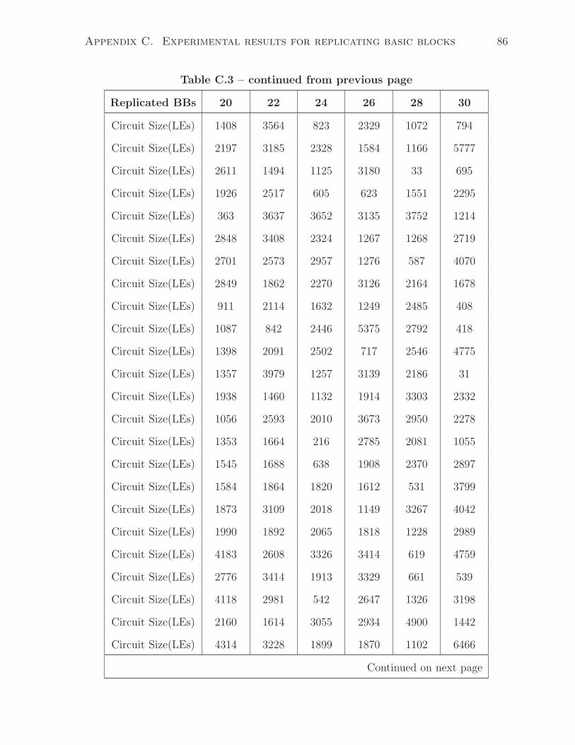
Appendix C. Experimental results for replicating basic blocks 86
Table C.3 – continued from previous page
Replicated BBs 20 22 24 26 28 30
Circuit Size(LEs) 1408 3564 823 2329 1072 794
Circuit Size(LEs) 2197 3185 2328 1584 1166 5777
Circuit Size(LEs) 2611 1494 1125 3180 33 695
Circuit Size(LEs) 1926 2517 605 623 1551 2295
Circuit Size(LEs) 363 3637 3652 3135 3752 1214
Circuit Size(LEs) 2848 3408 2324 1267 1268 2719
Circuit Size(LEs) 2701 2573 2957 1276 587 4070
Circuit Size(LEs) 2849 1862 2270 3126 2164 1678
Circuit Size(LEs) 911 2114 1632 1249 2485 408
Circuit Size(LEs) 1087 842 2446 5375 2792 418
Circuit Size(LEs) 1398 2091 2502 717 2546 4775
Circuit Size(LEs) 1357 3979 1257 3139 2186 31
Circuit Size(LEs) 1938 1460 1132 1914 3303 2332
Circuit Size(LEs) 1056 2593 2010 3673 2950 2278
Circuit Size(LEs) 1353 1664 216 2785 2081 1055
Circuit Size(LEs) 1545 1688 638 1908 2370 2897
Circuit Size(LEs) 1584 1864 1820 1612 531 3799
Circuit Size(LEs) 1873 3109 2018 1149 3267 4042
Circuit Size(LEs) 1990 1892 2065 1818 1228 2989
Circuit Size(LEs) 4183 2608 3326 3414 619 4759
Circuit Size(LEs) 2776 3414 1913 3329 661 539
Circuit Size(LEs) 4118 2981 542 2647 1326 3198
Circuit Size(LEs) 2160 1614 3055 2934 4900 1442
Circuit Size(LEs) 4314 3228 1899 1870 1102 6466
Continued on next page
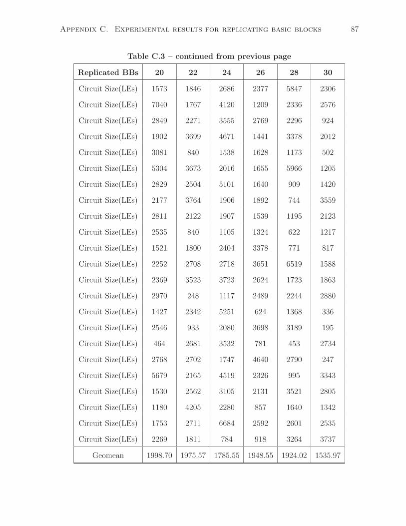
Appendix C. Experimental results for replicating basic blocks 87
Table C.3 – continued from previous page
Replicated BBs 20 22 24 26 28 30
Circuit Size(LEs) 1573 1846 2686 2377 5847 2306
Circuit Size(LEs) 7040 1767 4120 1209 2336 2576
Circuit Size(LEs) 2849 2271 3555 2769 2296 924
Circuit Size(LEs) 1902 3699 4671 1441 3378 2012
Circuit Size(LEs) 3081 840 1538 1628 1173 502
Circuit Size(LEs) 5304 3673 2016 1655 5966 1205
Circuit Size(LEs) 2829 2504 5101 1640 909 1420
Circuit Size(LEs) 2177 3764 1906 1892 744 3559
Circuit Size(LEs) 2811 2122 1907 1539 1195 2123
Circuit Size(LEs) 2535 840 1105 1324 622 1217
Circuit Size(LEs) 1521 1800 2404 3378 771 817
Circuit Size(LEs) 2252 2708 2718 3651 6519 1588
Circuit Size(LEs) 2369 3523 3723 2624 1723 1863
Circuit Size(LEs) 2970 248 1117 2489 2244 2880
Circuit Size(LEs) 1427 2342 5251 624 1368 336
Circuit Size(LEs) 2546 933 2080 3698 3189 195
Circuit Size(LEs) 464 2681 3532 781 453 2734
Circuit Size(LEs) 2768 2702 1747 4640 2790 247
Circuit Size(LEs) 5679 2165 4519 2326 995 3343
Circuit Size(LEs) 1530 2562 3105 2131 3521 2805
Circuit Size(LEs) 1180 4205 2280 857 1640 1342
Circuit Size(LEs) 1753 2711 6684 2592 2601 2535
Circuit Size(LEs) 2269 1811 784 918 3264 3737
Geomean 1998.70 1975.57 1785.55 1948.55 1924.02 1535.97

Appendix C. Experimental results for replicating basic blocks 88
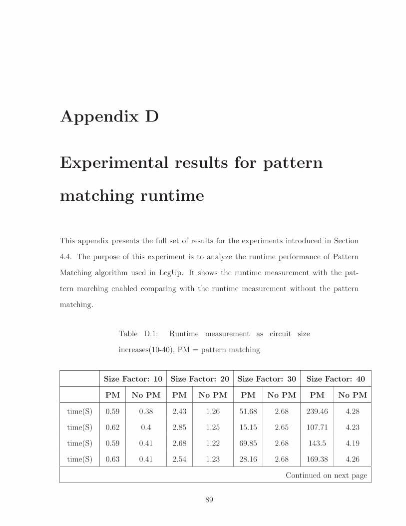
Appendix D
Experimental results for pattern
matching runtime
This appendix presents the full set of results for the experiments introduced in Section
4.4. The purpose of this experiment is to analyze the runtime performance of Pattern
Matching algorithm used in LegUp. It shows the runtime measurement with the pat-
tern marching enabled comparing with the runtime measurement without the pattern
matching.
Table D.1: Runtime measurement as circuit size
increases(10-40), PM = pattern matching
Size Factor: 10 Size Factor: 20 Size Factor: 30 Size Factor: 40
PM No PM PM No PM PM No PM PM No PM
time(S) 0.59 0.38 2.43 1.26 51.68 2.68 239.46 4.28
time(S) 0.62 0.4 2.85 1.25 15.15 2.65 107.71 4.23
time(S) 0.59 0.41 2.68 1.22 69.85 2.68 143.5 4.19
time(S) 0.63 0.41 2.54 1.23 28.16 2.68 169.38 4.26
Continued on next page
89
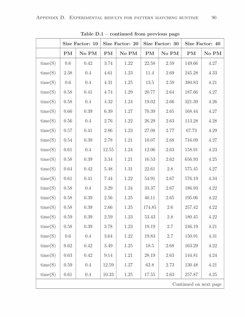
Appendix D. Experimental results for pattern matching runtime 90
Table D.1 – continued from previous page
Size Factor: 10 Size Factor: 20 Size Factor: 30 Size Factor: 40
PM No PM PM No PM PM No PM PM No PM
time(S) 0.6 0.42 3.74 1.22 22.58 2.59 149.66 4.27
time(S) 2.38 0.4 4.61 1.23 11.4 2.69 245.28 4.33
time(S) 0.6 0.4 4.31 1.25 13.5 2.59 380.83 4.21
time(S) 0.58 0.41 4.74 1.29 20.77 2.64 187.66 4.27
time(S) 0.58 0.4 4.32 1.24 19.02 2.66 321.39 4.26
time(S) 0.66 0.39 6.39 1.27 70.39 2.65 168.44 4.27
time(S) 0.56 0.4 2.76 1.22 26.29 2.63 113.28 4.28
time(S) 0.57 0.41 2.86 1.23 27.08 2.77 67.73 4.29
time(S) 0.54 0.39 2.78 1.21 10.07 2.68 716.09 4.27
time(S) 0.61 0.4 12.55 1.24 12.06 2.63 158.91 4.23
time(S) 0.58 0.39 3.34 1.21 16.53 2.62 656.93 4.25
time(S) 0.64 0.42 5.48 1.31 22.61 2.8 575.45 4.27
time(S) 0.61 0.41 7.44 1.22 54.91 2.67 576.19 4.34
time(S) 0.58 0.4 3.29 1.24 33.37 2.67 186.93 4.22
time(S) 0.58 0.39 2.56 1.25 40.11 2.65 195.06 4.22
time(S) 0.58 0.39 2.66 1.25 174.85 2.6 257.42 4.22
time(S) 0.59 0.39 2.59 1.23 53.43 2.8 180.45 4.22
time(S) 0.58 0.39 3.78 1.23 19.19 2.7 246.19 4.21
time(S) 0.6 0.4 3.64 1.22 19.83 2.7 150.91 4.31
time(S) 0.62 0.42 3.49 1.25 18.5 2.68 163.29 4.22
time(S) 0.63 0.42 9.14 1.21 28.19 2.63 144.81 4.24
time(S) 0.59 0.4 12.59 1.27 62.8 2.73 130.48 4.21
time(S) 0.61 0.4 10.33 1.25 17.55 2.63 257.87 4.25
Continued on next page
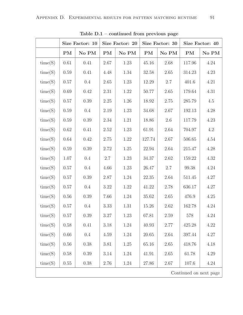
Appendix D. Experimental results for pattern matching runtime 91
Table D.1 – continued from previous page
Size Factor: 10 Size Factor: 20 Size Factor: 30 Size Factor: 40
PM No PM PM No PM PM No PM PM No PM
time(S) 0.61 0.41 2.67 1.23 45.16 2.68 117.96 4.24
time(S) 0.59 0.41 4.48 1.34 32.58 2.65 314.23 4.23
time(S) 0.57 0.4 2.65 1.23 12.29 2.7 401.6 4.21
time(S) 0.69 0.42 2.31 1.22 50.77 2.65 179.64 4.31
time(S) 0.57 0.39 2.25 1.26 18.92 2.75 285.79 4.5
time(S) 0.59 0.4 2.19 1.23 34.68 2.67 192.13 4.28
time(S) 0.59 0.39 2.34 1.21 18.86 2.6 117.79 4.23
time(S) 0.62 0.41 2.52 1.23 61.91 2.64 704.97 4.2
time(S) 0.64 0.42 2.75 1.22 127.74 2.67 506.65 4.54
time(S) 0.59 0.39 2.72 1.25 22.94 2.64 215.47 4.28
time(S) 1.07 0.4 2.7 1.23 34.37 2.62 159.22 4.32
time(S) 0.57 0.4 4.66 1.23 26.47 2.7 99.38 4.24
time(S) 0.57 0.39 2.87 1.24 22.35 2.64 511.45 4.27
time(S) 0.57 0.4 3.22 1.22 41.22 2.78 636.17 4.27
time(S) 0.56 0.39 7.66 1.24 35.62 2.65 476.9 4.25
time(S) 0.57 0.4 3.33 1.31 15.26 2.62 162.78 4.24
time(S) 0.57 0.39 3.27 1.23 67.81 2.59 578 4.24
time(S) 0.58 0.41 3.18 1.24 40.93 2.77 425.28 4.22
time(S) 0.66 0.4 4.59 1.24 20.65 2.64 397.44 4.27
time(S) 0.56 0.38 3.81 1.25 65.16 2.65 418.76 4.18
time(S) 0.58 0.39 3.14 1.24 41.91 2.65 61.78 4.29
time(S) 0.55 0.38 2.76 1.24 27.86 2.67 107.6 4.24
Continued on next page
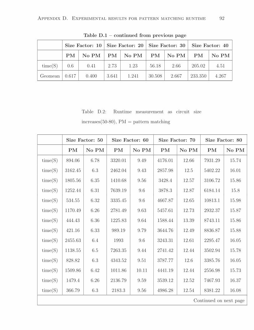
Appendix D. Experimental results for pattern matching runtime 92
Table D.1 – continued from previous page
Size Factor: 10 Size Factor: 20 Size Factor: 30 Size Factor: 40
PM No PM PM No PM PM No PM PM No PM
time(S) 0.6 0.41 2.73 1.23 56.18 2.66 205.02 4.51
Geomean 0.617 0.400 3.641 1.241 30.508 2.667 233.350 4.267
Table D.2: Runtime measurement as circuit size
increases(50-80), PM = pattern matching
Size Factor: 50 Size Factor: 60 Size Factor: 70 Size Factor: 80
PM No PM PM No PM PM No PM PM No PM
time(S) 894.06 6.78 3320.01 9.49 4176.01 12.66 7931.29 15.74
time(S) 3162.45 6.3 2462.04 9.43 2857.98 12.5 5402.22 16.01
time(S) 1805.56 6.35 1410.68 9.56 3428.4 12.57 3106.72 15.86
time(S) 1252.44 6.31 7639.19 9.6 3878.3 12.87 6184.14 15.8
time(S) 534.55 6.32 3335.45 9.6 4667.87 12.65 10813.1 15.98
time(S) 1170.49 6.26 2781.49 9.63 5457.61 12.73 2932.37 15.87
time(S) 444.43 6.36 1225.83 9.64 1588.44 13.39 8743.11 15.86
time(S) 421.16 6.33 989.19 9.79 3644.76 12.49 8836.87 15.88
time(S) 2455.63 6.4 1993 9.6 3243.31 12.61 2295.47 16.05
time(S) 1138.55 6.5 7263.35 9.44 2741.42 12.44 3502.94 15.78
time(S) 828.82 6.3 4343.52 9.51 3787.77 12.6 3385.76 16.05
time(S) 1509.86 6.42 1011.86 10.11 4441.19 12.44 2556.98 15.73
time(S) 1479.4 6.26 2136.79 9.59 3539.12 12.52 7467.93 16.37
time(S) 366.79 6.3 2183.3 9.56 4986.28 12.54 8381.22 16.08
Continued on next page
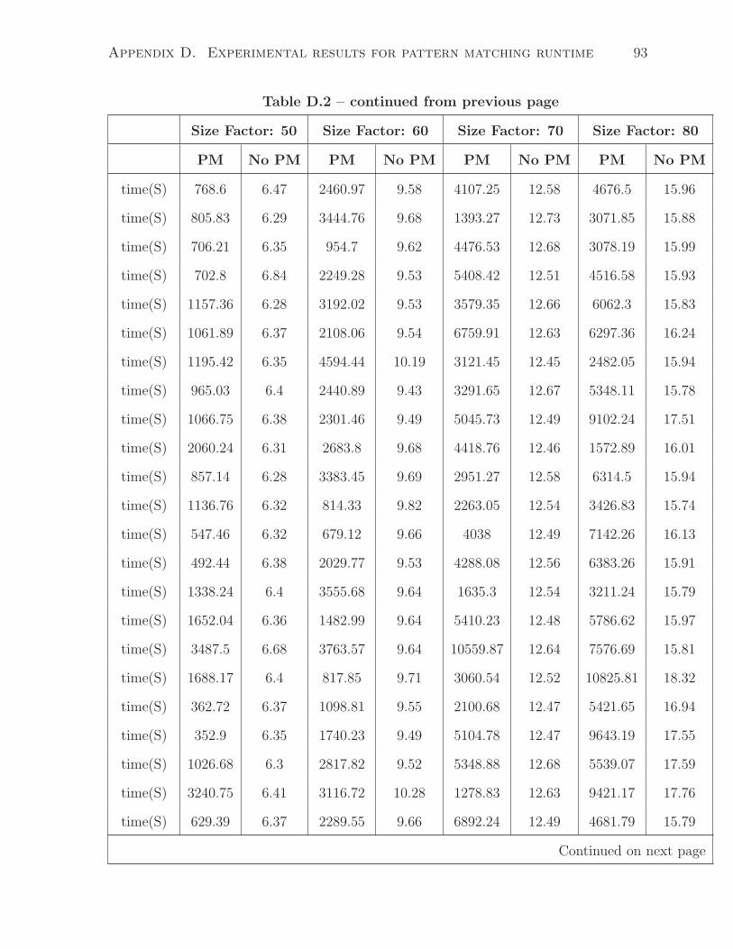
Appendix D. Experimental results for pattern matching runtime 93
Table D.2 – continued from previous page
Size Factor: 50 Size Factor: 60 Size Factor: 70 Size Factor: 80
PM No PM PM No PM PM No PM PM No PM
time(S) 768.6 6.47 2460.97 9.58 4107.25 12.58 4676.5 15.96
time(S) 805.83 6.29 3444.76 9.68 1393.27 12.73 3071.85 15.88
time(S) 706.21 6.35 954.7 9.62 4476.53 12.68 3078.19 15.99
time(S) 702.8 6.84 2249.28 9.53 5408.42 12.51 4516.58 15.93
time(S) 1157.36 6.28 3192.02 9.53 3579.35 12.66 6062.3 15.83
time(S) 1061.89 6.37 2108.06 9.54 6759.91 12.63 6297.36 16.24
time(S) 1195.42 6.35 4594.44 10.19 3121.45 12.45 2482.05 15.94
time(S) 965.03 6.4 2440.89 9.43 3291.65 12.67 5348.11 15.78
time(S) 1066.75 6.38 2301.46 9.49 5045.73 12.49 9102.24 17.51
time(S) 2060.24 6.31 2683.8 9.68 4418.76 12.46 1572.89 16.01
time(S) 857.14 6.28 3383.45 9.69 2951.27 12.58 6314.5 15.94
time(S) 1136.76 6.32 814.33 9.82 2263.05 12.54 3426.83 15.74
time(S) 547.46 6.32 679.12 9.66 4038 12.49 7142.26 16.13
time(S) 492.44 6.38 2029.77 9.53 4288.08 12.56 6383.26 15.91
time(S) 1338.24 6.4 3555.68 9.64 1635.3 12.54 3211.24 15.79
time(S) 1652.04 6.36 1482.99 9.64 5410.23 12.48 5786.62 15.97
time(S) 3487.5 6.68 3763.57 9.64 10559.87 12.64 7576.69 15.81
time(S) 1688.17 6.4 817.85 9.71 3060.54 12.52 10825.81 18.32
time(S) 362.72 6.37 1098.81 9.55 2100.68 12.47 5421.65 16.94
time(S) 352.9 6.35 1740.23 9.49 5104.78 12.47 9643.19 17.55
time(S) 1026.68 6.3 2817.82 9.52 5348.88 12.68 5539.07 17.59
time(S) 3240.75 6.41 3116.72 10.28 1278.83 12.63 9421.17 17.76
time(S) 629.39 6.37 2289.55 9.66 6892.24 12.49 4681.79 15.79
Continued on next page
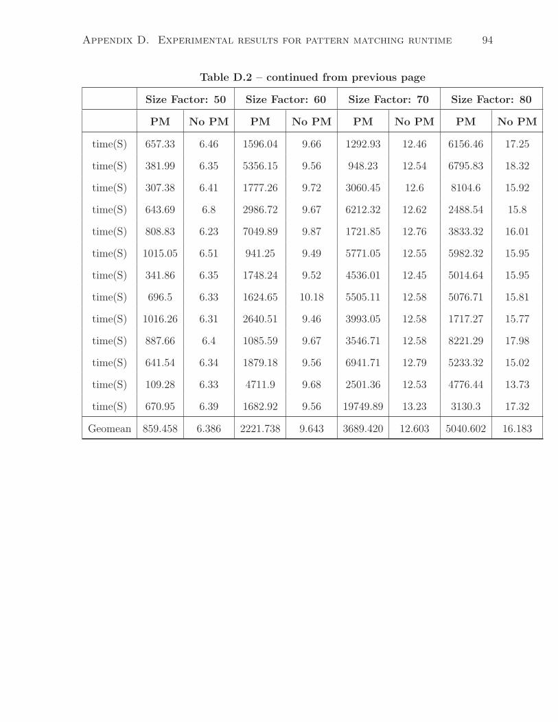
Appendix D. Experimental results for pattern matching runtime 94
Table D.2 – continued from previous page
Size Factor: 50 Size Factor: 60 Size Factor: 70 Size Factor: 80
PM No PM PM No PM PM No PM PM No PM
time(S) 657.33 6.46 1596.04 9.66 1292.93 12.46 6156.46 17.25
time(S) 381.99 6.35 5356.15 9.56 948.23 12.54 6795.83 18.32
time(S) 307.38 6.41 1777.26 9.72 3060.45 12.6 8104.6 15.92
time(S) 643.69 6.8 2986.72 9.67 6212.32 12.62 2488.54 15.8
time(S) 808.83 6.23 7049.89 9.87 1721.85 12.76 3833.32 16.01
time(S) 1015.05 6.51 941.25 9.49 5771.05 12.55 5982.32 15.95
time(S) 341.86 6.35 1748.24 9.52 4536.01 12.45 5014.64 15.95
time(S) 696.5 6.33 1624.65 10.18 5505.11 12.58 5076.71 15.81
time(S) 1016.26 6.31 2640.51 9.46 3993.05 12.58 1717.27 15.77
time(S) 887.66 6.4 1085.59 9.67 3546.71 12.58 8221.29 17.98
time(S) 641.54 6.34 1879.18 9.56 6941.71 12.79 5233.32 15.02
time(S) 109.28 6.33 4711.9 9.68 2501.36 12.53 4776.44 13.73
time(S) 670.95 6.39 1682.92 9.56 19749.89 13.23 3130.3 17.32
Geomean 859.458 6.386 2221.738 9.643 3689.420 12.603 5040.602 16.183
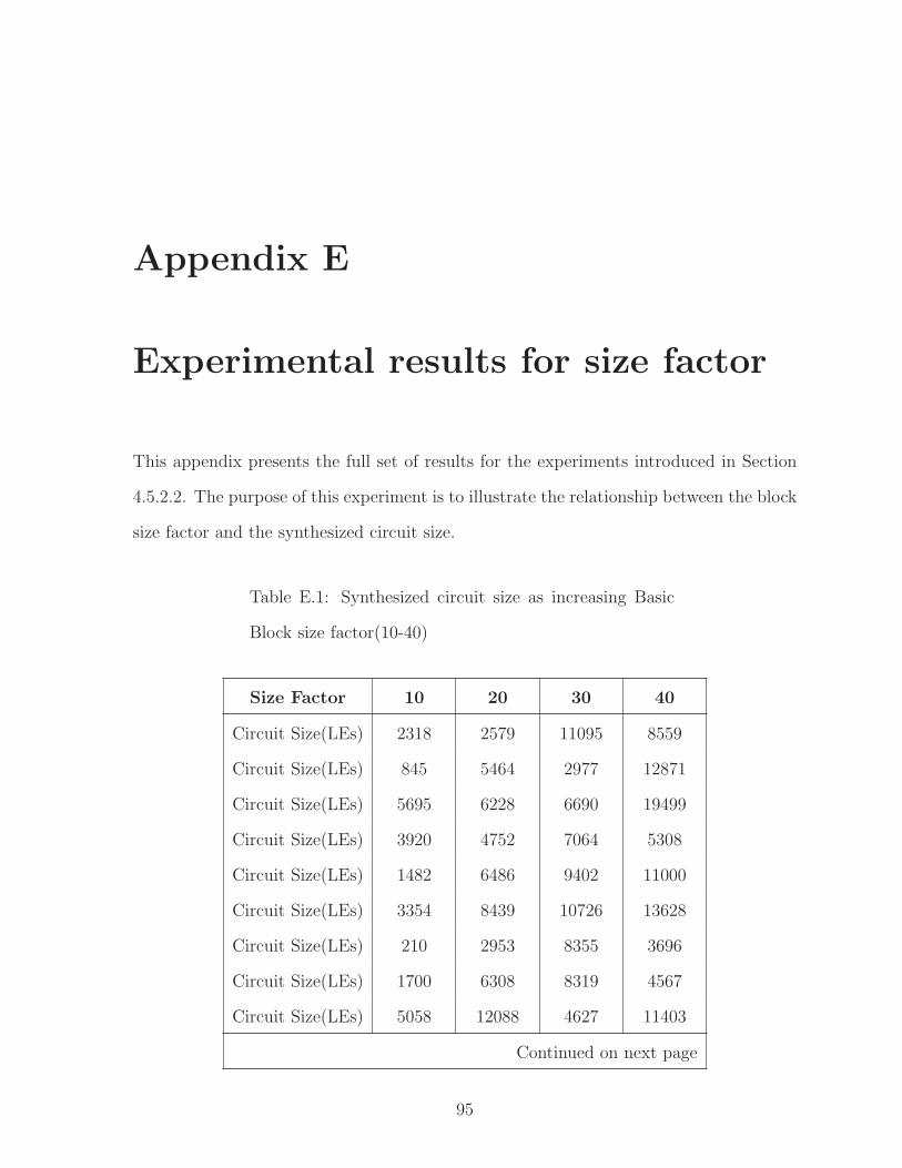
Appendix E
Experimental results for size factor
This appendix presents the full set of results for the experiments introduced in Section
4.5.2.2. The purpose of this experiment is to illustrate the relationship between the block
size factor and the synthesized circuit size.
Table E.1: Synthesized circuit size as increasing Basic
Block size factor(10-40)
Size Factor 10 20 30 40
Circuit Size(LEs) 2318 2579 11095 8559
Circuit Size(LEs) 845 5464 2977 12871
Circuit Size(LEs) 5695 6228 6690 19499
Circuit Size(LEs) 3920 4752 7064 5308
Circuit Size(LEs) 1482 6486 9402 11000
Circuit Size(LEs) 3354 8439 10726 13628
Circuit Size(LEs) 210 2953 8355 3696
Circuit Size(LEs) 1700 6308 8319 4567
Circuit Size(LEs) 5058 12088 4627 11403
Continued on next page
95
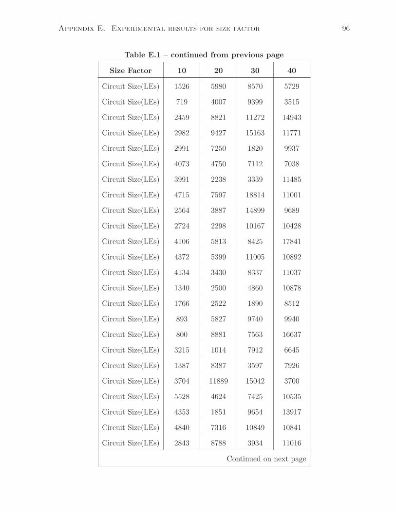
Appendix E. Experimental results for size factor 96
Table E.1 – continued from previous page
Size Factor 10 20 30 40
Circuit Size(LEs) 1526 5980 8570 5729
Circuit Size(LEs) 719 4007 9399 3515
Circuit Size(LEs) 2459 8821 11272 14943
Circuit Size(LEs) 2982 9427 15163 11771
Circuit Size(LEs) 2991 7250 1820 9937
Circuit Size(LEs) 4073 4750 7112 7038
Circuit Size(LEs) 3991 2238 3339 11485
Circuit Size(LEs) 4715 7597 18814 11001
Circuit Size(LEs) 2564 3887 14899 9689
Circuit Size(LEs) 2724 2298 10167 10428
Circuit Size(LEs) 4106 5813 8425 17841
Circuit Size(LEs) 4372 5399 11005 10892
Circuit Size(LEs) 4134 3430 8337 11037
Circuit Size(LEs) 1340 2500 4860 10878
Circuit Size(LEs) 1766 2522 1890 8512
Circuit Size(LEs) 893 5827 9740 9940
Circuit Size(LEs) 800 8881 7563 16637
Circuit Size(LEs) 3215 1014 7912 6645
Circuit Size(LEs) 1387 8387 3597 7926
Circuit Size(LEs) 3704 11889 15042 3700
Circuit Size(LEs) 5528 4624 7425 10535
Circuit Size(LEs) 4353 1851 9654 13917
Circuit Size(LEs) 4840 7316 10849 10841
Circuit Size(LEs) 2843 8788 3934 11016
Continued on next page
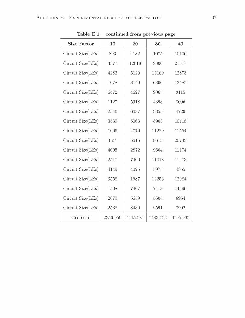
Appendix E. Experimental results for size factor 97
Table E.1 – continued from previous page
Size Factor 10 20 30 40
Circuit Size(LEs) 893 4182 1075 10106
Circuit Size(LEs) 3377 12018 9800 21517
Circuit Size(LEs) 4282 5120 12169 12873
Circuit Size(LEs) 1078 8149 6800 13585
Circuit Size(LEs) 6472 4627 9065 9115
Circuit Size(LEs) 1127 5918 4393 8096
Circuit Size(LEs) 2546 6687 9355 4729
Circuit Size(LEs) 3539 5063 8903 10118
Circuit Size(LEs) 1006 4779 11229 11554
Circuit Size(LEs) 627 5615 8613 20743
Circuit Size(LEs) 4695 2872 9604 11174
Circuit Size(LEs) 2517 7400 11018 11473
Circuit Size(LEs) 4149 4025 5975 4365
Circuit Size(LEs) 3558 1687 12256 12084
Circuit Size(LEs) 1508 7407 7418 14296
Circuit Size(LEs) 2679 5659 5605 6964
Circuit Size(LEs) 2538 8430 9591 8902
Geomean 2350.059 5115.581 7483.752 9705.935
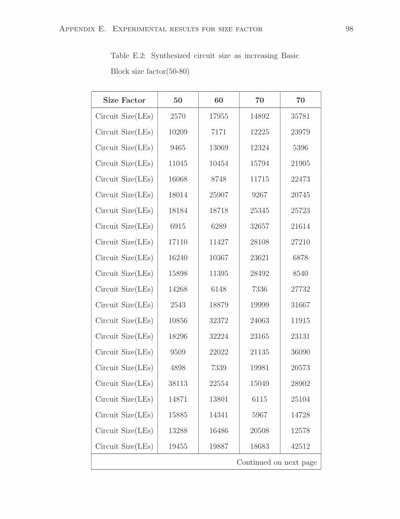
Appendix E. Experimental results for size factor 98
Table E.2: Synthesized circuit size as increasing Basic
Block size factor(50-80)
Size Factor 50 60 70 70
Circuit Size(LEs) 2570 17955 14892 35781
Circuit Size(LEs) 10209 7171 12225 23979
Circuit Size(LEs) 9465 13069 12324 5396
Circuit Size(LEs) 11045 10454 15794 21905
Circuit Size(LEs) 16068 8748 11715 22473
Circuit Size(LEs) 18014 25907 9267 20745
Circuit Size(LEs) 18184 18718 25345 25723
Circuit Size(LEs) 6915 6289 32657 21614
Circuit Size(LEs) 17110 11427 28108 27210
Circuit Size(LEs) 16240 10367 23621 6878
Circuit Size(LEs) 15898 11395 28492 8540
Circuit Size(LEs) 14268 6148 7336 27732
Circuit Size(LEs) 2543 18879 19999 31667
Circuit Size(LEs) 10856 32372 24063 11915
Circuit Size(LEs) 18296 32224 23165 23131
Circuit Size(LEs) 9509 22022 21135 36090
Circuit Size(LEs) 4898 7339 19981 20573
Circuit Size(LEs) 38113 22554 15049 28902
Circuit Size(LEs) 14871 13801 6115 25104
Circuit Size(LEs) 15885 14341 5967 14728
Circuit Size(LEs) 13288 16486 20508 12578
Circuit Size(LEs) 19455 19887 18683 42512
Continued on next page
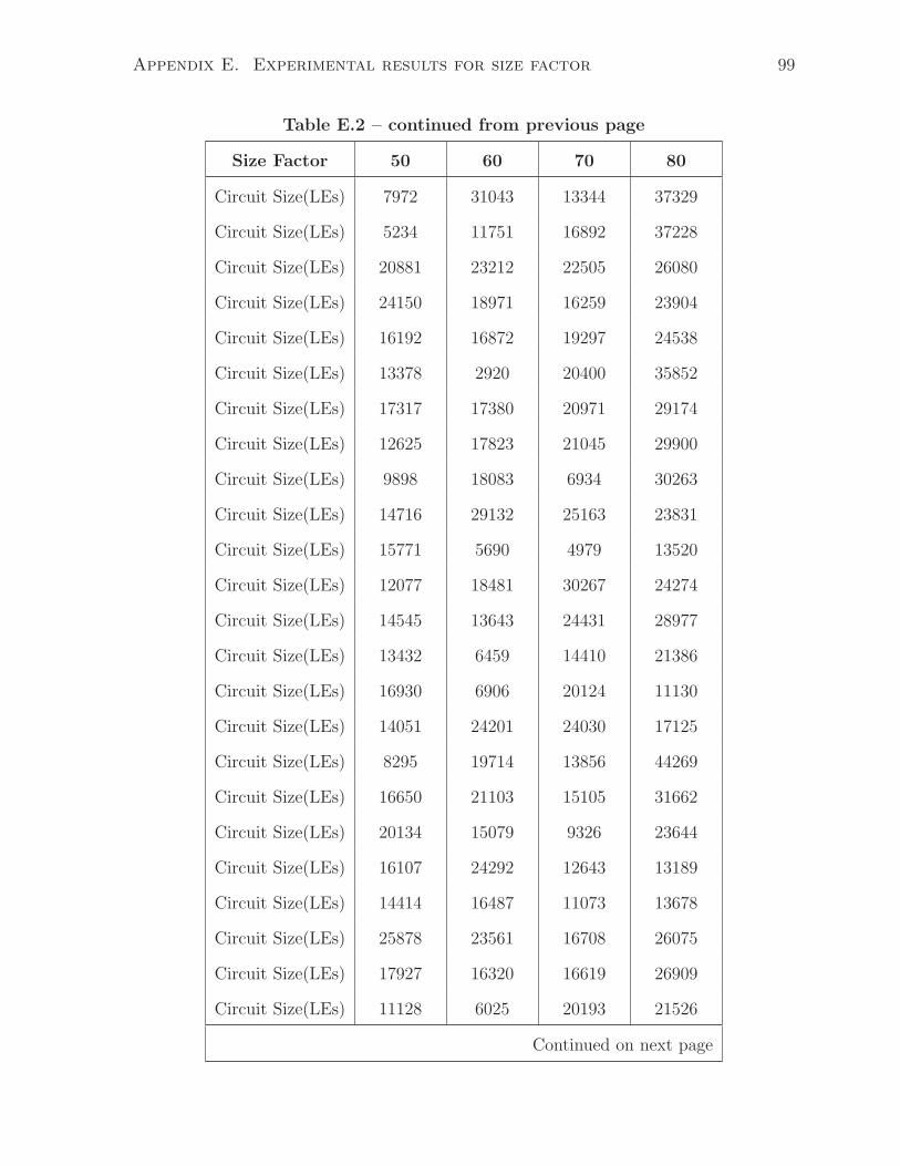
Appendix E. Experimental results for size factor 99
Table E.2 – continued from previous page
Size Factor 50 60 70 80
Circuit Size(LEs) 7972 31043 13344 37329
Circuit Size(LEs) 5234 11751 16892 37228
Circuit Size(LEs) 20881 23212 22505 26080
Circuit Size(LEs) 24150 18971 16259 23904
Circuit Size(LEs) 16192 16872 19297 24538
Circuit Size(LEs) 13378 2920 20400 35852
Circuit Size(LEs) 17317 17380 20971 29174
Circuit Size(LEs) 12625 17823 21045 29900
Circuit Size(LEs) 9898 18083 6934 30263
Circuit Size(LEs) 14716 29132 25163 23831
Circuit Size(LEs) 15771 5690 4979 13520
Circuit Size(LEs) 12077 18481 30267 24274
Circuit Size(LEs) 14545 13643 24431 28977
Circuit Size(LEs) 13432 6459 14410 21386
Circuit Size(LEs) 16930 6906 20124 11130
Circuit Size(LEs) 14051 24201 24030 17125
Circuit Size(LEs) 8295 19714 13856 44269
Circuit Size(LEs) 16650 21103 15105 31662
Circuit Size(LEs) 20134 15079 9326 23644
Circuit Size(LEs) 16107 24292 12643 13189
Circuit Size(LEs) 14414 16487 11073 13678
Circuit Size(LEs) 25878 23561 16708 26075
Circuit Size(LEs) 17927 16320 16619 26909
Circuit Size(LEs) 11128 6025 20193 21526
Continued on next page
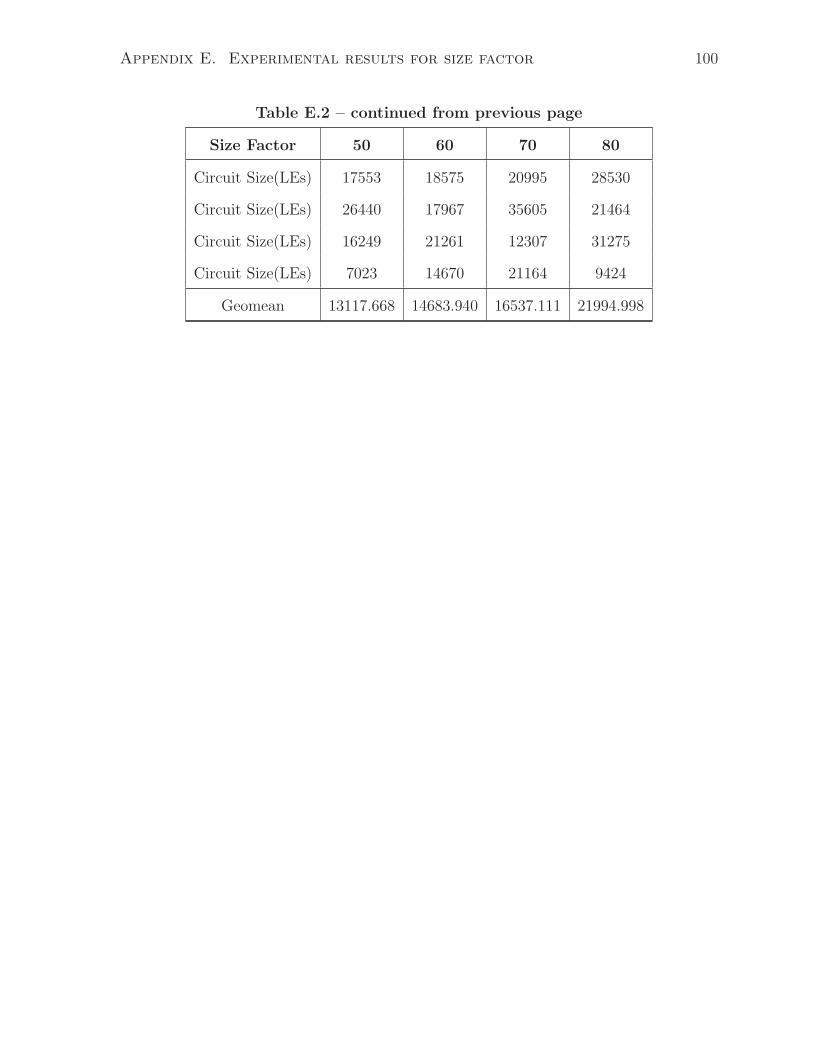
Appendix E. Experimental results for size factor 100
Table E.2 – continued from previous page
Size Factor 50 60 70 80
Circuit Size(LEs) 17553 18575 20995 28530
Circuit Size(LEs) 26440 17967 35605 21464
Circuit Size(LEs) 16249 21261 12307 31275
Circuit Size(LEs) 7023 14670 21164 9424
Geomean 13117.668 14683.940 16537.111 21994.998
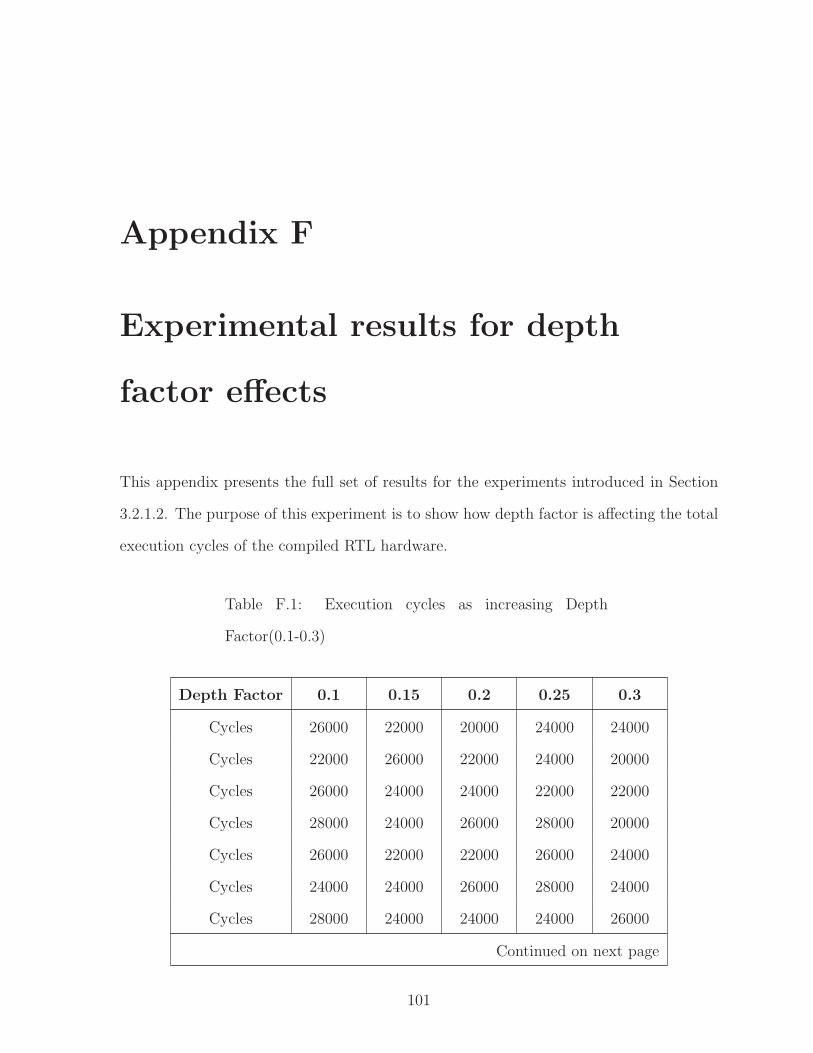
Appendix F
Experimental results for depth
factor effects
This appendix presents the full set of results for the experiments introduced in Section
3.2.1.2. The purpose of this experiment is to show how depth factor is affecting the total
execution cycles of the compiled RTL hardware.
Table F.1: Execution cycles as increasing Depth
Factor(0.1-0.3)
Depth Factor 0.1 0.15 0.2 0.25 0.3
Cycles 26000 22000 20000 24000 24000
Cycles 22000 26000 22000 24000 20000
Cycles 26000 24000 24000 22000 22000
Cycles 28000 24000 26000 28000 20000
Cycles 26000 22000 22000 26000 24000
Cycles 24000 24000 26000 28000 24000
Cycles 28000 24000 24000 24000 26000
Continued on next page
101
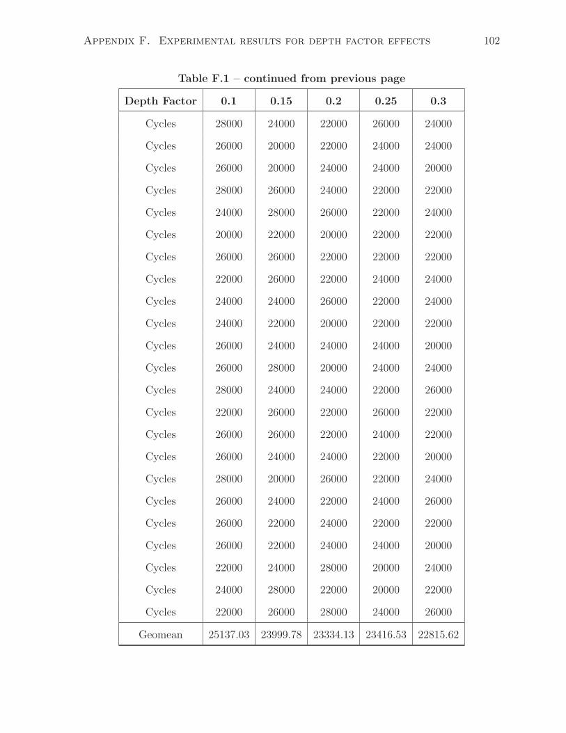
Appendix F. Experimental results for depth factor effects 102
Table F.1 – continued from previous page
Depth Factor 0.1 0.15 0.2 0.25 0.3
Cycles 28000 24000 22000 26000 24000
Cycles 26000 20000 22000 24000 24000
Cycles 26000 20000 24000 24000 20000
Cycles 28000 26000 24000 22000 22000
Cycles 24000 28000 26000 22000 24000
Cycles 20000 22000 20000 22000 22000
Cycles 26000 26000 22000 22000 22000
Cycles 22000 26000 22000 24000 24000
Cycles 24000 24000 26000 22000 24000
Cycles 24000 22000 20000 22000 22000
Cycles 26000 24000 24000 24000 20000
Cycles 26000 28000 20000 24000 24000
Cycles 28000 24000 24000 22000 26000
Cycles 22000 26000 22000 26000 22000
Cycles 26000 26000 22000 24000 22000
Cycles 26000 24000 24000 22000 20000
Cycles 28000 20000 26000 22000 24000
Cycles 26000 24000 22000 24000 26000
Cycles 26000 22000 24000 22000 22000
Cycles 26000 22000 24000 24000 20000
Cycles 22000 24000 28000 20000 24000
Cycles 24000 28000 22000 20000 22000
Cycles 22000 26000 28000 24000 26000
Geomean 25137.03 23999.78 23334.13 23416.53 22815.62
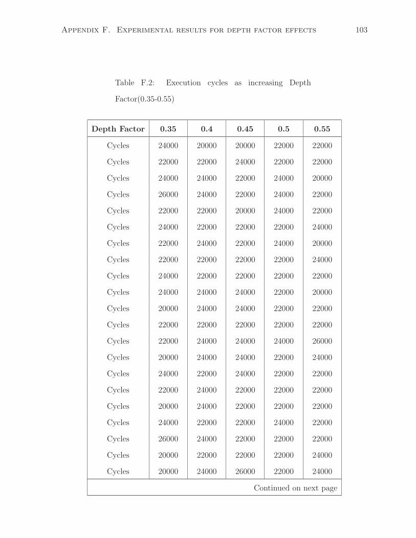
Appendix F. Experimental results for depth factor effects 103
Table F.2: Execution cycles as increasing Depth
Factor(0.35-0.55)
Depth Factor 0.35 0.4 0.45 0.5 0.55
Cycles 24000 20000 20000 22000 22000
Cycles 22000 22000 24000 22000 22000
Cycles 24000 24000 22000 24000 20000
Cycles 26000 24000 22000 24000 22000
Cycles 22000 22000 20000 24000 22000
Cycles 24000 22000 22000 22000 24000
Cycles 22000 24000 22000 24000 20000
Cycles 22000 22000 22000 22000 24000
Cycles 24000 22000 22000 22000 22000
Cycles 24000 24000 24000 22000 20000
Cycles 20000 24000 24000 22000 22000
Cycles 22000 22000 22000 22000 22000
Cycles 22000 24000 24000 24000 26000
Cycles 20000 24000 24000 22000 24000
Cycles 24000 22000 24000 22000 22000
Cycles 22000 24000 22000 22000 22000
Cycles 20000 24000 22000 22000 22000
Cycles 24000 22000 22000 24000 22000
Cycles 26000 24000 22000 22000 22000
Cycles 20000 22000 22000 22000 24000
Cycles 20000 24000 26000 22000 24000
Continued on next page
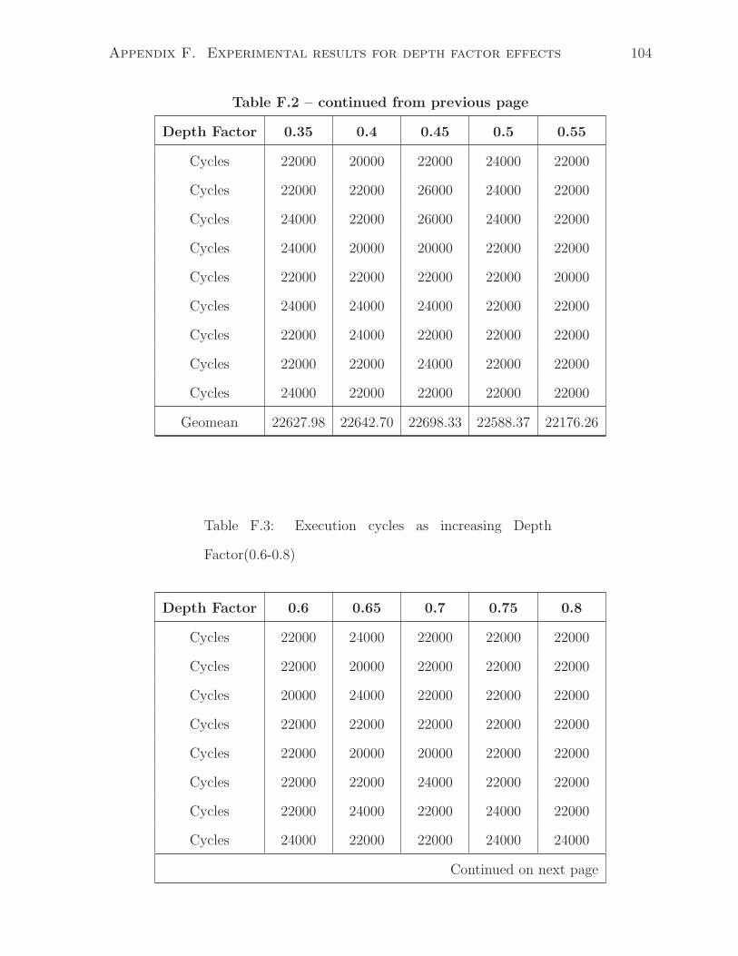
Appendix F. Experimental results for depth factor effects 104
Table F.2 – continued from previous page
Depth Factor 0.35 0.4 0.45 0.5 0.55
Cycles 22000 20000 22000 24000 22000
Cycles 22000 22000 26000 24000 22000
Cycles 24000 22000 26000 24000 22000
Cycles 24000 20000 20000 22000 22000
Cycles 22000 22000 22000 22000 20000
Cycles 24000 24000 24000 22000 22000
Cycles 22000 24000 22000 22000 22000
Cycles 22000 22000 24000 22000 22000
Cycles 24000 22000 22000 22000 22000
Geomean 22627.98 22642.70 22698.33 22588.37 22176.26
Table F.3: Execution cycles as increasing Depth
Factor(0.6-0.8)
Depth Factor 0.6 0.65 0.7 0.75 0.8
Cycles 22000 24000 22000 22000 22000
Cycles 22000 20000 22000 22000 22000
Cycles 20000 24000 22000 22000 22000
Cycles 22000 22000 22000 22000 22000
Cycles 22000 20000 20000 22000 22000
Cycles 22000 22000 24000 22000 22000
Cycles 22000 24000 22000 24000 22000
Cycles 24000 22000 22000 24000 24000
Continued on next page
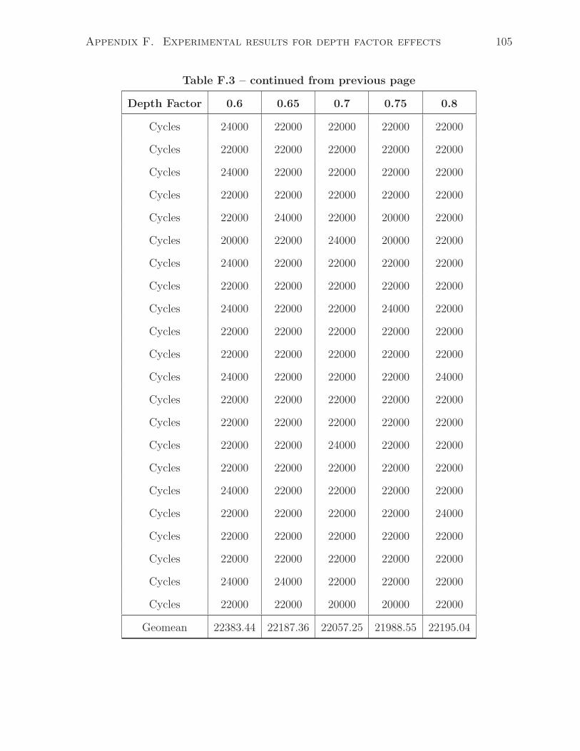
Appendix F. Experimental results for depth factor effects 105
Table F.3 – continued from previous page
Depth Factor 0.6 0.65 0.7 0.75 0.8
Cycles 24000 22000 22000 22000 22000
Cycles 22000 22000 22000 22000 22000
Cycles 24000 22000 22000 22000 22000
Cycles 22000 22000 22000 22000 22000
Cycles 22000 24000 22000 20000 22000
Cycles 20000 22000 24000 20000 22000
Cycles 24000 22000 22000 22000 22000
Cycles 22000 22000 22000 22000 22000
Cycles 24000 22000 22000 24000 22000
Cycles 22000 22000 22000 22000 22000
Cycles 22000 22000 22000 22000 22000
Cycles 24000 22000 22000 22000 24000
Cycles 22000 22000 22000 22000 22000
Cycles 22000 22000 22000 22000 22000
Cycles 22000 22000 24000 22000 22000
Cycles 22000 22000 22000 22000 22000
Cycles 24000 22000 22000 22000 22000
Cycles 22000 22000 22000 22000 24000
Cycles 22000 22000 22000 22000 22000
Cycles 22000 22000 22000 22000 22000
Cycles 24000 24000 22000 22000 22000
Cycles 22000 22000 20000 20000 22000
Geomean 22383.44 22187.36 22057.25 21988.55 22195.04
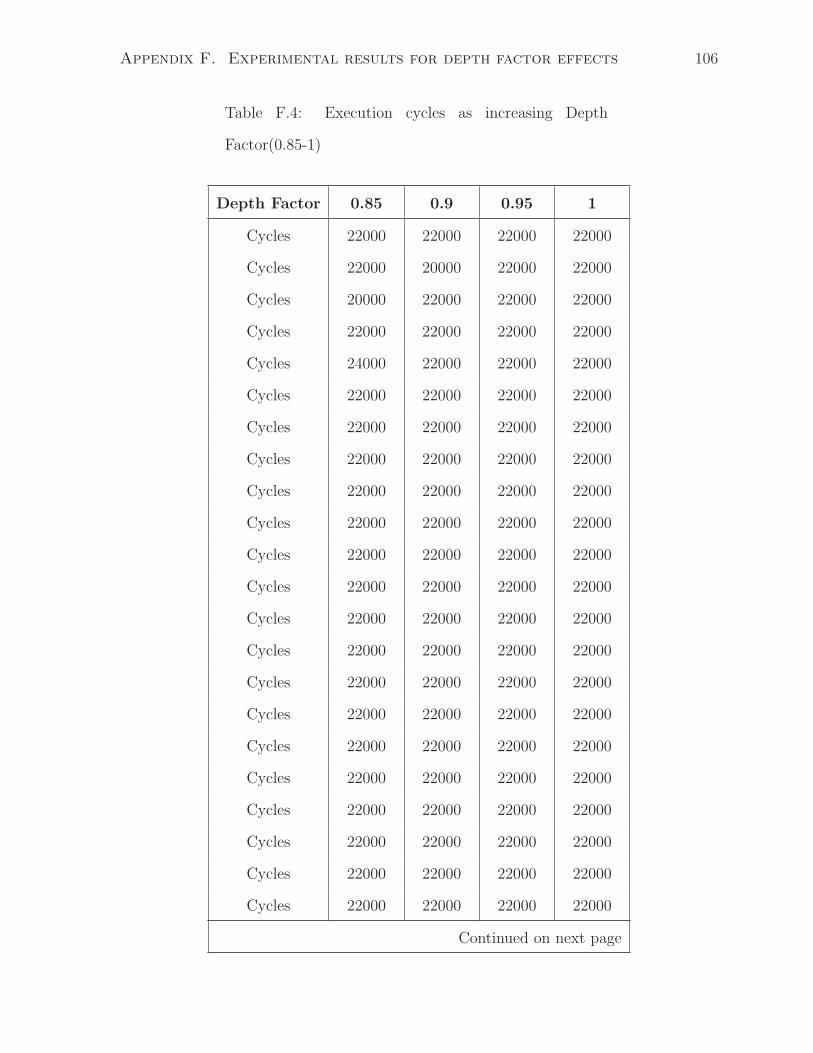
Appendix F. Experimental results for depth factor effects 106
Table F.4: Execution cycles as increasing Depth
Factor(0.85-1)
Depth Factor 0.85 0.9 0.95 1
Cycles 22000 22000 22000 22000
Cycles 22000 20000 22000 22000
Cycles 20000 22000 22000 22000
Cycles 22000 22000 22000 22000
Cycles 24000 22000 22000 22000
Cycles 22000 22000 22000 22000
Cycles 22000 22000 22000 22000
Cycles 22000 22000 22000 22000
Cycles 22000 22000 22000 22000
Cycles 22000 22000 22000 22000
Cycles 22000 22000 22000 22000
Cycles 22000 22000 22000 22000
Cycles 22000 22000 22000 22000
Cycles 22000 22000 22000 22000
Cycles 22000 22000 22000 22000
Cycles 22000 22000 22000 22000
Cycles 22000 22000 22000 22000
Cycles 22000 22000 22000 22000
Cycles 22000 22000 22000 22000
Cycles 22000 22000 22000 22000
Cycles 22000 22000 22000 22000
Cycles 22000 22000 22000 22000
Continued on next page
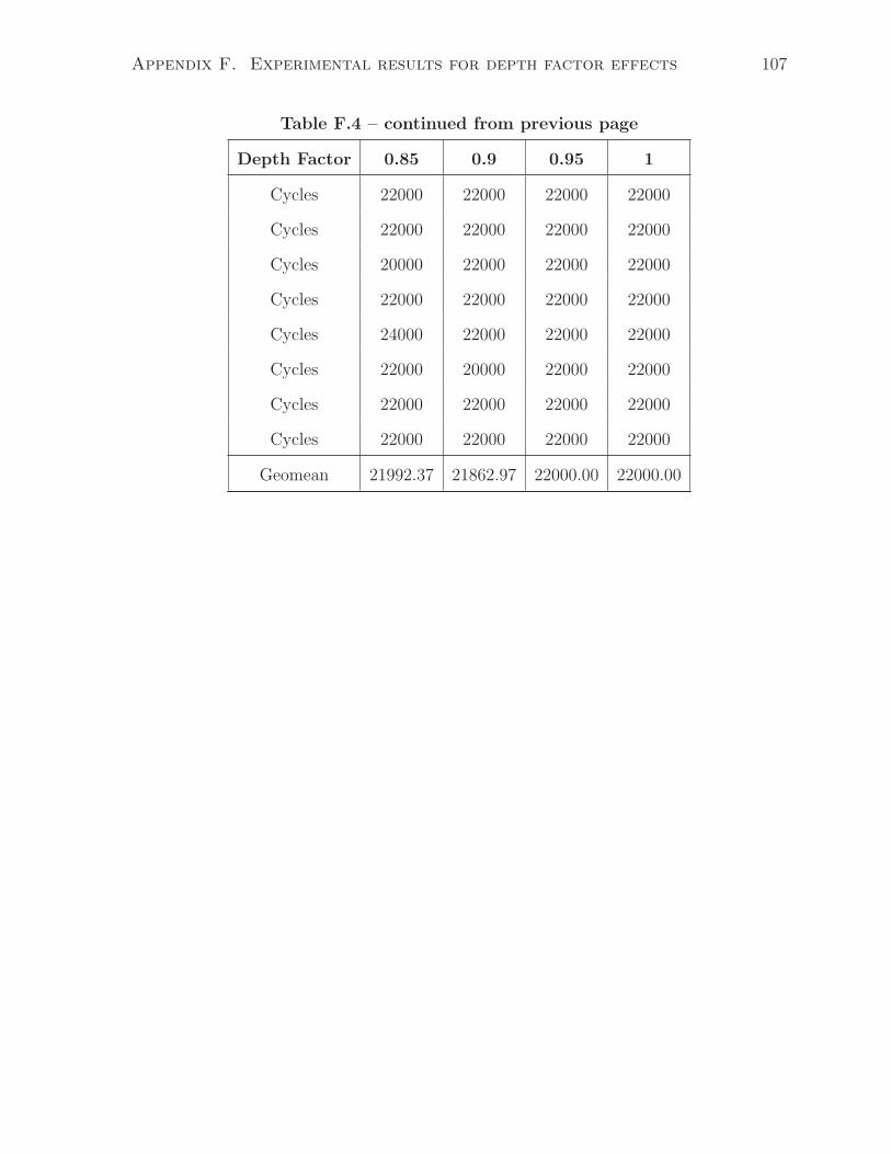
Appendix F. Experimental results for depth factor effects 107
Table F.4 – continued from previous page
Depth Factor 0.85 0.9 0.95 1
Cycles 22000 22000 22000 22000
Cycles 22000 22000 22000 22000
Cycles 20000 22000 22000 22000
Cycles 22000 22000 22000 22000
Cycles 24000 22000 22000 22000
Cycles 22000 20000 22000 22000
Cycles 22000 22000 22000 22000
Cycles 22000 22000 22000 22000
Geomean 21992.37 21862.97 22000.00 22000.00
Bibliography
[1] DOT language. http://en.wikipedia.org/wiki/DOT_language, 2012.
[2] Gcov - Using the GNU Compiler Collection (GCC). http://gcc.gnu.org/
onlinedocs/gcc/Gcov.html, 2012.
[3] LLVM Language Reference Manual. http://llvm.org/docs/LangRef.html, 2012.
[4] Standard Performance Evaluation Corporation: SPEC. http://www.spec.org/,
2012.
[5] The Embedded Microprocessor Benchmark Consortium: EEMBC. http://www.
eembc.org/, 2012.
[6] R. Camposano. Path-based scheduling for synthesis. In IEEE J CAD, pages 85–93,
1991.
[7] A. Canis, J. Choi, M. Aldham, V. Zhang, A. Kammoona, J.H. Anderson,
S. Brown, and T. Czajkowski. LegUp: High-level synthesis for FPGA-based pro-
cessor/accelerator systems. ACM/SIGDA International Symposium on Field Pro-
grammable Gate Arrays (FPGA), pages 33–36, 2011.
[8] Edmund Clarke, Daniel Kroening, and Karen Yorav. Behavioral Consistency of C
and Verilog Programs Using Bounded Model Checking. In DAC, pages 368–371,
2003.
108
Bibliography 109
[9] Stephen A. Cook. The complexity of theorem-proving procedures. In Proceedings of
the 3rd Annual ACM Symposium on Theory of Computing, pages 151–158, 1971.
[10] Philippe Coussy and Adam Morawiec. High-Level Synthesis From Algorithm to
Digital Circuit. Springer, 2008.
[11] John A. Curreri. Performance analysis and verification for high-level synthesis. In
UNIVERSITY OF FLORIDA, 2011.
[12] S. Hadjis; A. Canis; J.H. Anderson; J. Choi; K. Nam; S. Brown; T. Cza-
jkowski. Impact of FPGA Architecture on Resource Sharing in High-Level Synthe-
sis. In ACM/SIGDA International Symposium on Field Programmable Gate Arrays
(FPGA), 2012.
[13] Gary Smith Grant Martin. High-Level Synthesis: Past, Present, and Future. In
IEEE Design and Test of Computers, pages 18–25, 2009.
[14] Y. Hara.; H. Tomiyama ; S. Honda; H.akada. Proposal and quantitative analysis of
the CHStone benchmark program suite for practical C-based high-level synthesis.
In Journal of Information Processing 17, pages 242–254, 2009.
[15] K.S. Hemmert. A class of polynomially solvable range constraints for interval analy-
sis without widenings. In Field-Programmable Custom Computing Machines, 2003,
pages 228–237, 2003.
[16] Chandan Karfa; D. Sarkar; C. Mandal; P. Kumar. An Equivalence-Checking Method
for Scheduling Verication in High-Level Synthesis. In IEEE J CAD, pages 556–569,
2008.
[17] V. Lattner, C.; Adve. LLVM: a compilation framework for lifelong program anal-
ysis & transformation. In Code Generation and Optimization, 2004. CGO 2004.
International Symposium, pages 75–86, 2004.
Bibliography 110
[18] Chunho Lee; Miodrag Potkonjak; William H. Mangione-Smith. MediaBench: a tool
for evaluating and synthesizing multimedia and communicatons systems. In Proceed-
ings of the 30th annual ACM/IEEE international symposium on Microarchitecture,
pages 330–335, 1997.
[19] Steven S. Muchnick. Advanced Compiler Design and Implementation. Morgan Kauf-
mann, 1997.
[20] S. Gupta; N. Savoiu; N. Dutt; R. Gupta; A. Nicolau. Using global code motions
to improve the quality of results for high-level synthesis. In IEEE J CAD, pages
302–312, 2004.
[21] D.N. Panda, R.P; Dutt. 1995 High Level Synthesis Design Repository. In Interna-
tional Symposium on System Synthesis, pages 170–174, 1995.
[22] Nikil D Dutt; Champaka Ramachandran. Benchmarks for the 1992 high level syn-
thesis workshop. In Technical Report, University of California, Irvine, pages 92–107,
1992.
[23] P. Coussy; D.D. Gajski; M. Meredith; A. Takach. An Introduction to High-Level
Synthesis. In IEEE M DTC, pages 8–17, 2009.
[24] Igor Rafael de Assis Costa Victor Hugo Sperle Campos, Raphael Ernani Rodrigues
and Fernando Magno Quinto Pereira. Speed and Precision in Range Analysis. In
Brazilian Symposium on Programming Languages, 2012.
[25] Zhendong Su; David Wagner. Source level debugger for the Sea Cucumber synthe-
sizing compiler. In Theoretical Computer Science, pages 122–138, 2005.
[26] Kazutoshi Wakabayashi. C-based SoC Design Flow and EDA Tools: An ASIC and
System Vendor Perspective. In IEEE Trans. Computer-Aided Design of Integrated
Circuits and Systems, pages 1507–1522, 2000.