AUTOMATED CAMERA TRACKING SYSTEM IN GAIT ANALYSIS

MASTER THESIS

NOVEMBER 21, 2016 BISWAS LOHANI V K, MASTER IN ENGINEERING (BIOMEDICAL)

FLINDERS UNIVERSITY

11/21/2016

Master Thesis | Biswas Lohani V K

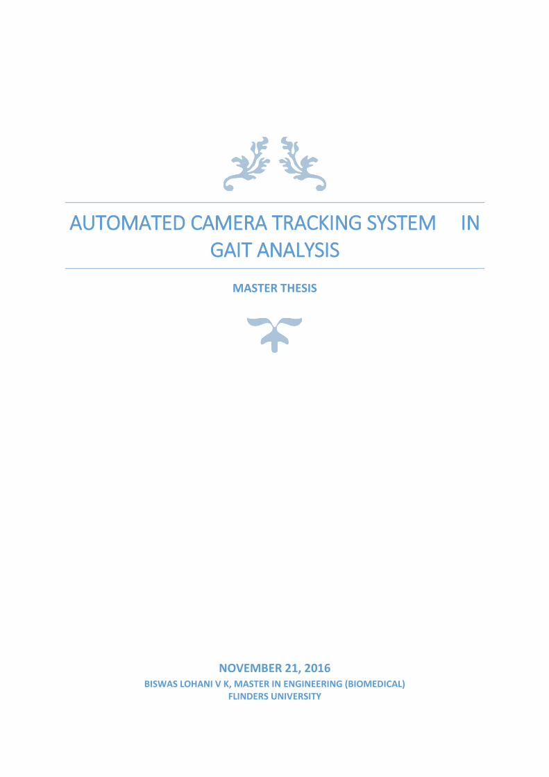
PROJECT AUTOMATED TRACKING CAMERA SYSTEM

IN GAIT ANALYSIS Dr Benjamin Patritti

Researcher

Repatriation General Hospital

Dr Olivia Lockwood

Supervisor

School of Medicine

Dr Sherry Randhawa

Academic Supervisor

School of Computer Science, Engineering and Mathematics

i

Declaration

I certify that this work does not incorporate without acknowledgment any material previously

submitted for a degree or diploma in any university; and that to the best of my knowledge and

belief, it does not contain any material previously published or written by another person

except where due reference is made in the text.

______________________ Author: Biswas Lohani V K

Signature 11/21/2016

ii

Preface

This master’s thesis has been conducted at the School of Computer Science, Engineering and

Mathematics, Flinders University as the partial fulfillment for the requirement of the degree

program. It is a visual sensitivity to control a four-wheel drive robot by tracking the position

of patient with color or people as input object during the Gait Analysis.

iii

Abstract

People have numerous walking abnormalities due to the certain illness or medical condition. The

main reason is due to the muscle or neurological issues. Hence, the scope of Clinical Gait

Analysis (CGA) arises to measure and estimate the gait biomechanics, which makes it easier to

recognize the abnormal appearances during the Gait Analysis and it also helps to make the

accurate clinical decision regarding orthopedic surgery and rehabilitation for the clinician.

There are different techniques to collect the motion related information during the Gait Analysis.

In which, recording of good quality video has the significant role in the CGA process which

visualize the walking pattern of the patient immediately and the recorded video data can be

utilized a number of times during the gait analysis process as well as it can be used as reference

video information for the future assessment of the same patient.

Therefore, the project “Automated Camera Tracking System in Gait Analysis” is related to the

movement of the video recording camera along with the patient so that it could capture the

patient’s gait in different time intervals. This project is the advancement of the current system in

the Gait Lab of Repartition General Hospital, South Australia. The present system is the still

camera that has been used to capture the video of the walking patient from the side and front in

the walkway. This camera is not able to record more than a stride of a patient during the process

which is not sufficient to make an accurate clinical decision.

Consequently, in this master thesis, it has been proposed to build an automated four wheeled

drive robot which is operated to keep the object in sight by maintaining a steady perpendicular

distance between the system and the patient. Furthermore, different object detection and tracking

methods are implemented to focus a patient in the video with the automated camera tracking

system. Furthermore, the experimental analysis of the automated tracking system by using the

object detection and tracking method in image processing shows that the Histogram of Oriented

Gradient Features (HOGs) extraction methods for object detection and tracking is more effective

in this project because it gives more precise location data due to the locally normalized

histogram of gradient orientation features of an object which is also not affected by the

iv

environmental condition ( light, temperature etc.) in the Gait Lab and it also has less variation in

its speed so probability of losing patient from the focus is less in this method and the system can

move smoothly. On the other hand, the color object detection and tracking method is relatively

less effective in comparison with HOGs method of object detection and tracking due to the

fluctuation that occurs in object detection. This method not able to identify the exact location of

the object when used in the poor light conditions inside the Gait Lab but due to the low

computational cost it is implemented in the system by improving the brightness of light source in

the current Gait Lab.

v

Acknowledgement

I would like to thank those people who made this master thesis possible.

First of all, I greatly appreciate the help of my Academic Supervisor, Dr. Sherry Randhawa,

Supervisor, Dr. Olivia Lockwood & Researcher, Dr. Benjamin Patritti who advised and

encouraged me all way during this thesis work. I specially thank all of my supervisors for

their infinite patience. The discussions I had with them were invaluable. In addition, I would

like to thank Dr. Benjamin Patritti & His team from Repartition General Hospital for

providing the space in their gait lab during the testing of project work.

I want to say a big thank to Damian Kleiss, Craig Peacock & Richard Stanley from the

technical department for kindly providing me the requested parts and components as well as

for helping to design the track for driving the four-wheel drive robot. Also, I would like to

say special thanks to Amirmehdi Yazdani, PhD student, for sharing his knowledge to control

the robot at the desired speed and Nilen Man Shakya who always motivated me to work hard

to achieve the goal.

Besides, I am grateful to all the Flinders University staff and students who generously

contributed directly or indirectly during this thesis work.

My final words go to my family. I want to thank my family for their love and support all

these years.

Biswas Lohani V K, Flinders University, 11/21/2016

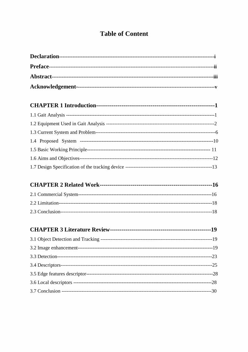
Table of Content

Declaration---------------------------------------------------------------------------------------------i

Preface---------------------------------------------------------------------------------------------------ii

Abstract-------------------------------------------------------------------------------------------------iii

Acknowledgement-----------------------------------------------------------------------------------v

CHAPTER 1 Introduction-------------------------------------------------------------1

1.1 Gait Analysis -----------------------------------------------------------------------------------------1

1.2 Equipment Used in Gait Analysis -----------------------------------------------------------------2

1.3 Current System and Problem------------------------------------------------------------------------6

1.4 Proposed System --------------------------------------------------------------------------------10

1.5 Basic Working Principle-------------------------------------------------------------------------- 11

1.6 Aims and Objectives--------------------------------------------------------------------------------12

1.7 Design Specification of the tracking device ----------------------------------------------------13

CHAPTER 2 Related Work----------------------------------------------------------16

2.1 Commercial System--------------------------------------------------------------------------------16

2.2 Limitation--------------------------------------------------------------------------------------------18

2.3 Conclusion-------------------------------------------------------------------------------------------18

CHAPTER 3 Literature Review----------------------------------------------------19

3.1 Object Detection and Tracking -------------------------------------------------------------------19

3.2 Image enhancement---------------------------------------------------------------------------------19

3.3 Detection---------------------------------------------------------------------------------------------23

3.4 Descriptors-------------------------------------------------------------------------------------------25

3.5 Edge features descriptor----------------------------------------------------------------------------28

3.6 Local descriptors -----------------------------------------------------------------------------------28

3.7 Conclusion ------------------------------------------------------------------------------------------30

CHAPTER 4 Fundamentals of Robotics------------------------------------------31

4.1 Introduciton------------------------------------------------------------------------------------------31

4.1.1 Parts of Robotcs------------------------------------------------------------------------------32

4.1.2 Total Estimated & Final Cost----------------------------------------------------------------41

4.2 Conclusion ------------------------------------------------------------------------------------------43

CHAPTER 5 Implementation and Analysis of Object Detection and

Tracking Method-----------------------------------------------------------------------44

5.1 Color object detection and tracking in image processing--------------------------------------44

5.1.1 Introduction-------------------------------------------------------------------------------------44

5.1.2 Colour object detection and tracking method----------------------------------------------44

5.1.3 Experimental Analysis of object detection and tracking---------------------------------51

5.2 Histogram of Oriented Gradient (HOGs) Methods for People Detection-------------------57

5.2.1 Introduction-------------------------------------------------------------------------------------57

5.2.2 Steps involved in histogram of oriented gradients methods------------------------------58

5.2.3 Experimental Analysis of HOGs Method for People Detection-------------------------66

5.2.4 Experimental result ---------------------------------------------------------------------------68

5. 3 Automated camera tracking system controller-------------------------------------------------69

5.4 Result & Discussion--------------------------------------------------------------------------------77

CHAPTER 6 Conclusions and Future Work-------------------------------------81

6.1 Conclusion-------------------------------------------------------------------------------------------81

6.2 Future work -----------------------------------------------------------------------------------------82

REFERENCE

APPENDIX 1 Object Detection & Tracking Matlab Code

APPENDIX 2 Control of robot with Arduino UNO, L298 DC Motor Driver, Arduino

Code

APPENDIX 3 Numerical calculation for colour segmentation method analysis

APPENDIX 4 Numerical calculation for HOGs analysis

APPENDIX 5 Circuit Diagram

List of Figure

Figure 1.1: Clinical gait analysis with multiple cameras in the gait lab.

Figure 1.2: Showing the location of marker sets prior to the Gait Analysis

Figure 1.3: Some of motion capture cameras used in the 3D gait analysis for capturing the

motion

Figure 1.4: Force plate example

Figure 1.5: High speed camera example

Figure 1.6: Current system used in the gait lab, General Repatriation Hospital, South

Australia

Figure 1.7: Two different FOV from different location in 2D gait Analysis

Figure 1.8: The still camera only able to focus within its range

Figure 1.9: Patient walking on FOV and capturing video showing on the monitor

Figure 1.10: Patient walks away from the FOV, absences of the patient in the video

Figure 1.11: Video capturing technique placing the camera at different position

Figure 1.12: Video gait analysis in the narrow space Gait Lab

Figure 1.13: Purposed 4WD Camera tracking system along with the patient

Figure 1.14: Continuous capturing of the patient walking

Figure 1.15: Block Diagram showing the working principle of the proposed system

Figure 1.16: Tracking System overview

Figure 2.1 Camera in a dolly in Monash Health, Victoria

Figure 2.2 Control box for the movement of the sliding camera

Figure 2.3: TeleGlide Track System, 2015

Figure 2.4: Ball bearing wheel

Figure 3.1: Contrast correction Top: Original, bottom: correction

Figure 3.2: Effect of Gaussian Blur on methods like edge detection. Left: Too much blur,

Middle: No blurs good edges, Right: Original image

Figure 3.3: Gaussian Blur Left: Too much blur, Right: Original image

Figure 3.4: Size, appearance in both images is similar for different sized objects.

Figure 3.5: Image pyramid with scaling of 20% for each step.

Figure 3.6: Harris point detector, detecting points in images with different viewpoints

Figure 3.7: Haar-like features for face detection

Figure 3.8: Face detection using Viola- Jones features

Figure 3.9: Some of the examples detecting the blue, red and green colored object

Figure 3.10: Example of how a local descriptor method, like SIFT, GLOH or SURF can be

used in detection of objects

Figure 4.1: Overview of components used in the system

Figure 4.2: 4WD Robotic platform

Figure 4.3 (a): Camera tracking system with linear bearing and motorized wheel

Figure 4.3 (b): Belt operated motorized tracking system

Figure 4.5: Raspberry Pi microcontroller development kit

Figure 4.6 Microcontroller development Kit Arduino UNO ATmega328 and with main pin

In/out

Figure 4.7: DVS128 and eDVS image sensor

Figure 4.8: OV7670 Image sensor

Figure 4.9: Overview of the CMUcam5 Pixy Camera

Figure 4.9: Connection of CMUcam5 Pixy Camera and Arduino UNO microcontroller

development board

Figure 4.10(a): Before selecting a colour object in a Pixy

Figure 4.10(b): After selecting a colour object in a Pixy

Figure 4.10(c): During the colour detection and tracking process selecting a colour object in a

Pixy Mon

Figure 4.11: Testing of CMUcam5 Pixy Camera for the object detection and tracking in the

Lab.

Figure 4.12(a, b c): Some of the custom made motor controller used to control the DC motor

Figure 4.13: Showing different connection with L298N DC Driver Motor

Figure 4.14: DC Driver Motors and wheels used in the automated tracking camera system.

Figure 4.15: 65mm wheel is selected for to run the motor

Figure 4.16: Bottom view of the robot showing the structure of DC Motor’s Connection.

Figure 4.17: Automated camera tracking system during the testing in Gait Lab, General

Repatriation Hospital, 2016

Figure 5.1: Block Diagram of colour object detection with histogram thresholding

Figure 5.2: Red, Green and Blue components taken from a 24- bit RGB images.

Figure 5.3: Steps involves in Histogram thresholding

Figure 5.4 (a) Binary image after thresholding (b) Detected colour object inside the box.

Figure 5.5: Transformation of the object p from one position to another.

Figure 5.6: Horizontal and vertical projections in binary image.

Figure 5.7: Standard Force plate measurement

Figure 5.8: Standard Force plate pit manual measurement in the Gait Lab

Figure 5.9: Matlab run time GUI development in the LAB. Top Left: colour object as t-shirt

detection and tracking, bottom Left: the Speed- Time Graph of the detected object and

bottom Right: Distance- Time Graph of the detected object.

Figure 5. 10: Block diagram shows the step involve in IA Method

Figure 5.11: Speed –Time Graph of the object being tracked and more stable portion of it

with red dotted box.

Figure 5.12: Block diagram showing the overall features extraction and detection chain

Figure5.13: Original Image taken in the Gait Lab, Repatriation General Hospital during

testing of HOGs people detection

Figure5.14 (a): Showing the oriented gradient vector in the image

Figure5.14 (b): 8x8 cell pixel cells within the detection window

Figure5.14(c): The gradient histogram within each cell

Figure 5.15: 9 Bin- histogram which ranges from 0 to 180.

Figure 5.16 (a, b, c, d): Example of normalization gradient vector

Figure 5.17: Gradient vector calculation

Figure 5.18 (a, b): Example showing the block normalization

Figure 19: Hard margin (solid line) and Soft margin (dotted line) SVM Classifier.

Figure 5.20: People detection with HOGs in real time

Figure 5.21: Over all overview of the Histogram Oriented Gradients (HOGs) feature

extraction

Figure 5.22: Matlab run time GUI development in the LAB. Top left: tracking of people by

HOGs feature extraction method in recorded video, bottom left: the speed- time graph of the

detected person and bottom right: distance- time graph of the detected person.

Figure 5.23: Shows the Speed time graph of the tracking object.

Figure 5.24: Flow chart to illustrate the structure of the code

Figure 5.25: Side View of object from the Camera targeting its initial position.

Figure 5.26: Initial position of the Robot with CMUcam5 Pixy Camera and colour object in

the right

Figure 5.27: (a) Division of pixel values in two sections where PIXYMON is the application

software for CMUcam5 Pixy camera to visualize a detected object.

(b) Showing the position of the same object in real view.

Figure 5.28: Tracking a colour object attached within the person's right leg same as in the

Figure (b)), x=160, Robot action: STOP

Figure 5.29: Tracking a colour object attached within the person left leg (same object as in

the Figure (b)), x<160, Robot action: LEFT

Figure 5.30: Tracking a colour object attached within the person's right leg same as in the

Figure (b)), x>160, Robot action: RIGHT

Figure 5.31: Showing the important Pin In/Pin Out in L298N DC Motor Driver

Figure: 5.32: Hardware connection of the Automated Tracking Camera System

Figure 5.33: Automated Tracking camera system after assembling

Figure 5.34: Overview final ready to use automated camera system

Figure 35: Comparison of average speed from FA Method and average speed from IA Method

Figure 5.36: Comparison of average speed from frame analysis and average speed from

image processing by using HOGs feature extraction.

Figure 5.37: The single frame of experimented video which shows the multiple location

within the same detected object by colour object detection and tracking method.

Figure 5. 38: The single frame of experimented video in the people is detected in the poor

light condition and low image resolution

.

Figure 6.1: Newly design automated tracking camera System (Front) &

Previous fixed side camera system (Back)

Figure 6.2: 4WD Robot control with smart phone application

Figure 6.3: Tracking of person with automated camera tracking system from both sides of the

patient

List of Table

Table 4.1: Overall estimated cost for the tracking system

Table 4.2: Total final cost after completion of the project

Table 5.1: Direction control with the L298N DC Motor controller

Table 5.2: Technical specification

Table 5.3: Comparing average speed from FA and IA with its difference in percentage.

Table 5.4: Comparing average speed from frame analysis and image processing with

observed error in percentage

Table 5.5: Comparison between HOGs and Colour segmentation performance

Table 5.6: Comparison of average speed, error from HOGs & Colour segmentation

1 | P a g e

CHAPTER 1 Introduction

1.1 Gait Analysis

Gait analysis can be defined in a number of ways. At the beginning John Saunders,

Verne Inman and Howard Elberhart started the ideas about the gait analysis

around 1952 with the six determinants of gait theory (R. Baker, 2013). Since after

that, thousands of papers have been published regarding gait analysis. In 2003,

Michael Whittle defined the gait analysis as “the organized measurement of

people walking, with the eye as well as brain of qualified observer, improved by

instrumentation for evaluating the motion of body, body mechanics and the action

of the muscles” (M. Whittle, 2003). He also stated that depending on the persons

with different circumstances disturbing their capability to walk, gait analysis may

be used to make comprehensive diagnoses and to map optimal care.

Later on in 2006, Prof. Chris Kirtley defined gait analysis in his book Clinical gait

analysis, theory and practice as “ gait analysis is a technique of locomotion

characterized by periods of loading and unloading of the limb”. While this

includes running, hopping, skipping and perhaps even swimming and cycling,

walking is the most frequently used gait, providing independence and used for

many of the activities of daily living (ADLs). It also facilitates any public

activities and is essential in many occupations (C. Kirtley, 2006). Likewise, “ gait

analysis is the process of determining what is causing patients to walk they do” (R.

Baker, 2013). He also mentioned in his book that it is based on the instrumented

measurement and a biomedical interpretation of what these measurements mean.

In over all, gait analysis is the organized measurement of animal locomotion, more

categorically the measurement of human walking, by utilizing the eye and the

brain of observers, improved by instrumentation for evaluating body motion, body

mechanics and the activity of the muscles.

2 | P a g e

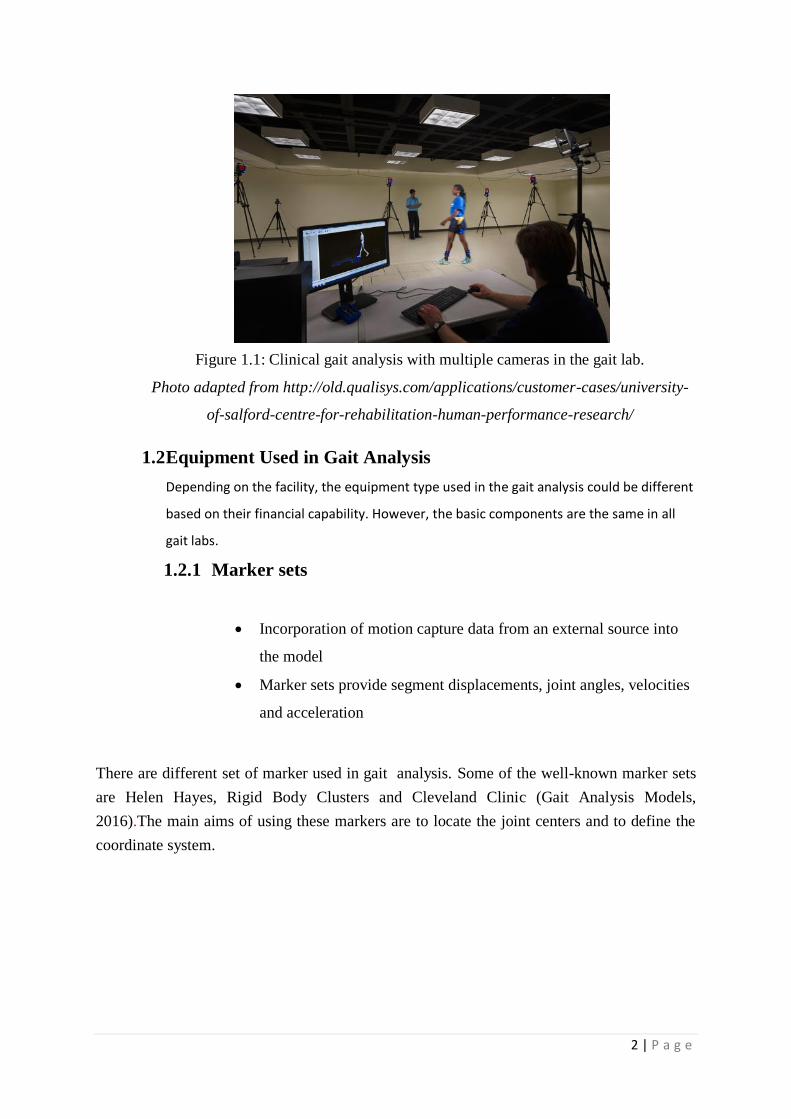
Figure 1.1: Clinical gait analysis with multiple cameras in the gait lab.

Photo adapted from http://old.qualisys.com/applications/customer-cases/university-

of-salford-centre-for-rehabilitation-human-performance-research/

1.2 Equipment Used in Gait Analysis

Depending on the facility, the equipment type used in the gait analysis could be different

based on their financial capability. However, the basic components are the same in all

gait labs.

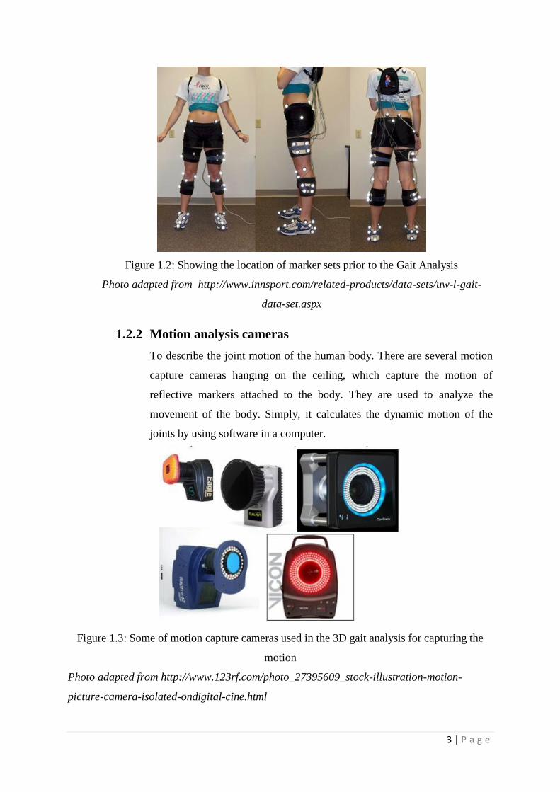
1.2.1 Marker sets

Incorporation of motion capture data from an external source into

the model

Marker sets provide segment displacements, joint angles, velocities

and acceleration

There are different set of marker used in gait analysis. Some of the well-known marker sets

are Helen Hayes, Rigid Body Clusters and Cleveland Clinic (Gait Analysis Models,

2016).The main aims of using these markers are to locate the joint centers and to define the

coordinate system.

3 | P a g e

Figure 1.2: Showing the location of marker sets prior to the Gait Analysis

Photo adapted from http://www.innsport.com/related-products/data-sets/uw-l-gait-

data-set.aspx

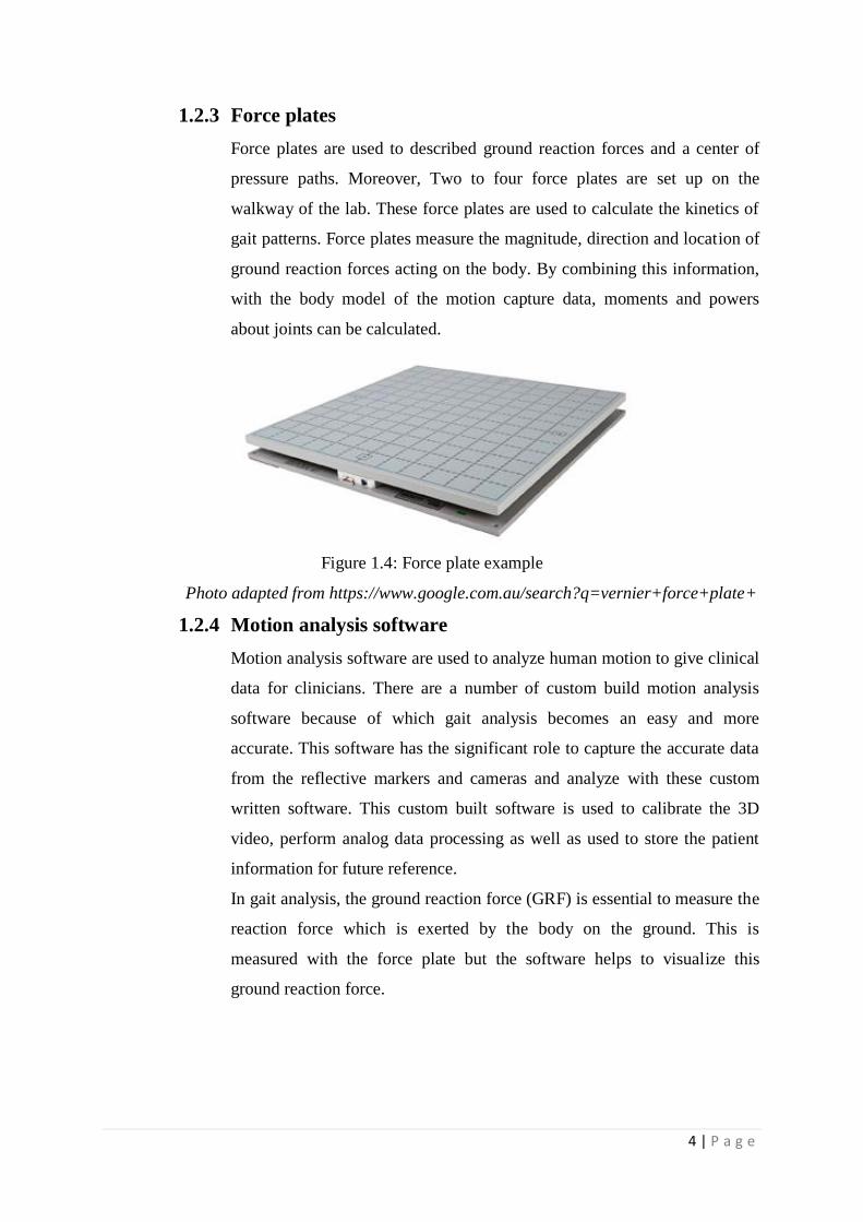
1.2.2 Motion analysis cameras

To describe the joint motion of the human body. There are several motion

capture cameras hanging on the ceiling, which capture the motion of

reflective markers attached to the body. They are used to analyze the

movement of the body. Simply, it calculates the dynamic motion of the

joints by using software in a computer.

Figure 1.3: Some of motion capture cameras used in the 3D gait analysis for capturing the

motion

Photo adapted from http://www.123rf.com/photo_27395609_stock-illustration-motion-

picture-camera-isolated-ondigital-cine.html

4 | P a g e

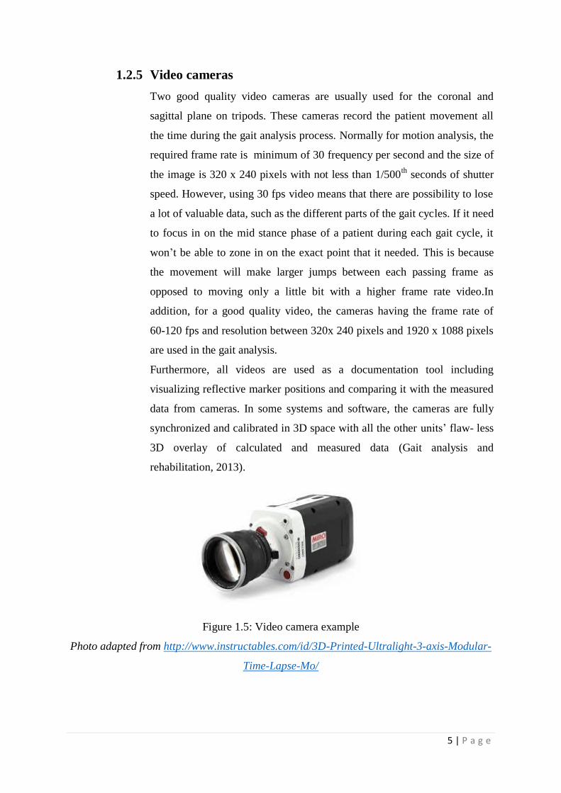
1.2.3 Force plates

Force plates are used to described ground reaction forces and a center of

pressure paths. Moreover, Two to four force plates are set up on the

walkway of the lab. These force plates are used to calculate the kinetics of

gait patterns. Force plates measure the magnitude, direction and location of

ground reaction forces acting on the body. By combining this information,

with the body model of the motion capture data, moments and powers

about joints can be calculated.

Figure 1.4: Force plate example

Photo adapted from https://www.google.com.au/search?q=vernier+force+plate+

1.2.4 Motion analysis software

Motion analysis software are used to analyze human motion to give clinical

data for clinicians. There are a number of custom build motion analysis

software because of which gait analysis becomes an easy and more

accurate. This software has the significant role to capture the accurate data

from the reflective markers and cameras and analyze with these custom

written software. This custom built software is used to calibrate the 3D

video, perform analog data processing as well as used to store the patient

information for future reference.

In gait analysis, the ground reaction force (GRF) is essential to measure the

reaction force which is exerted by the body on the ground. This is

measured with the force plate but the software helps to visualize this

ground reaction force.

5 | P a g e

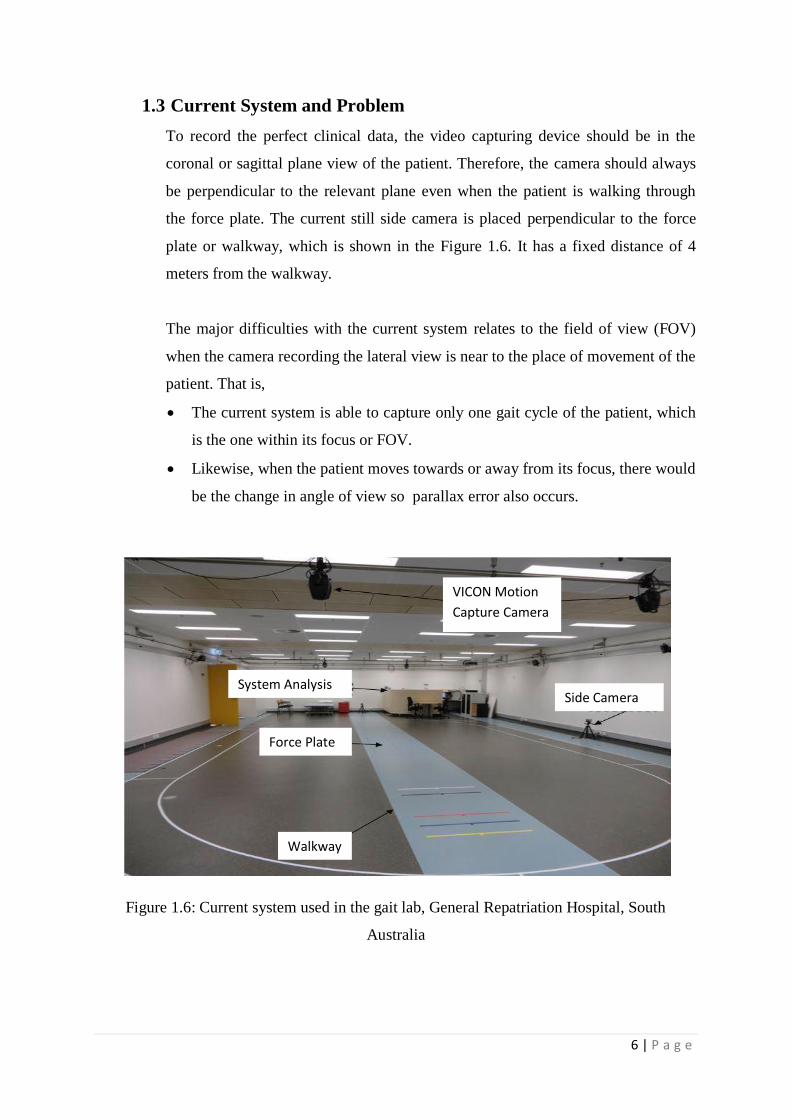
1.2.5 Video cameras

Two good quality video cameras are usually used for the coronal and

sagittal plane on tripods. These cameras record the patient movement all

the time during the gait analysis process. Normally for motion analysis, the

required frame rate is minimum of 30 frequency per second and the size of

the image is 320 x 240 pixels with not less than 1/500th

seconds of shutter

speed. However, using 30 fps video means that there are possibility to lose

a lot of valuable data, such as the different parts of the gait cycles. If it need

to focus in on the mid stance phase of a patient during each gait cycle, it

won’t be able to zone in on the exact point that it needed. This is because

the movement will make larger jumps between each passing frame as

opposed to moving only a little bit with a higher frame rate video.In

addition, for a good quality video, the cameras having the frame rate of

60-120 fps and resolution between 320x 240 pixels and 1920 x 1088 pixels

are used in the gait analysis.

Furthermore, all videos are used as a documentation tool including

visualizing reflective marker positions and comparing it with the measured

data from cameras. In some systems and software, the cameras are fully

synchronized and calibrated in 3D space with all the other units’ flaw- less

3D overlay of calculated and measured data (Gait analysis and

rehabilitation, 2013).

Figure 1.5: Video camera example

Photo adapted from http://www.instructables.com/id/3D-Printed-Ultralight-3-axis-Modular-

Time-Lapse-Mo/

6 | P a g e

1.3 Current System and Problem

To record the perfect clinical data, the video capturing device should be in the

coronal or sagittal plane view of the patient. Therefore, the camera should always

be perpendicular to the relevant plane even when the patient is walking through

the force plate. The current still side camera is placed perpendicular to the force

plate or walkway, which is shown in the Figure 1.6. It has a fixed distance of 4

meters from the walkway.

The major difficulties with the current system relates to the field of view (FOV)

when the camera recording the lateral view is near to the place of movement of the

patient. That is,

The current system is able to capture only one gait cycle of the patient, which

is the one within its focus or FOV.

Likewise, when the patient moves towards or away from its focus, there would

be the change in angle of view so parallax error also occurs.

Figure 1.6: Current system used in the gait lab, General Repatriation Hospital, South

Australia

System Analysis

VICON Motion

Capture Camera

Force Plate

Side Camera

Walkway

7 | P a g e

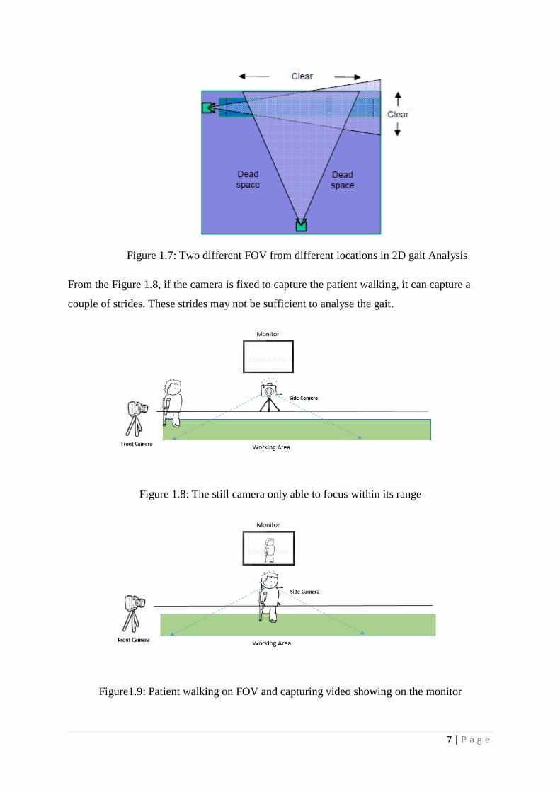
Figure 1.7: Two different FOV from different locations in 2D gait Analysis

From the Figure 1.8, if the camera is fixed to capture the patient walking, it can capture a

couple of strides. These strides may not be sufficient to analyse the gait.

Figure 1.8: The still camera only able to focus within its range

Figure1.9: Patient walking on FOV and capturing video showing on the monitor

8 | P a g e

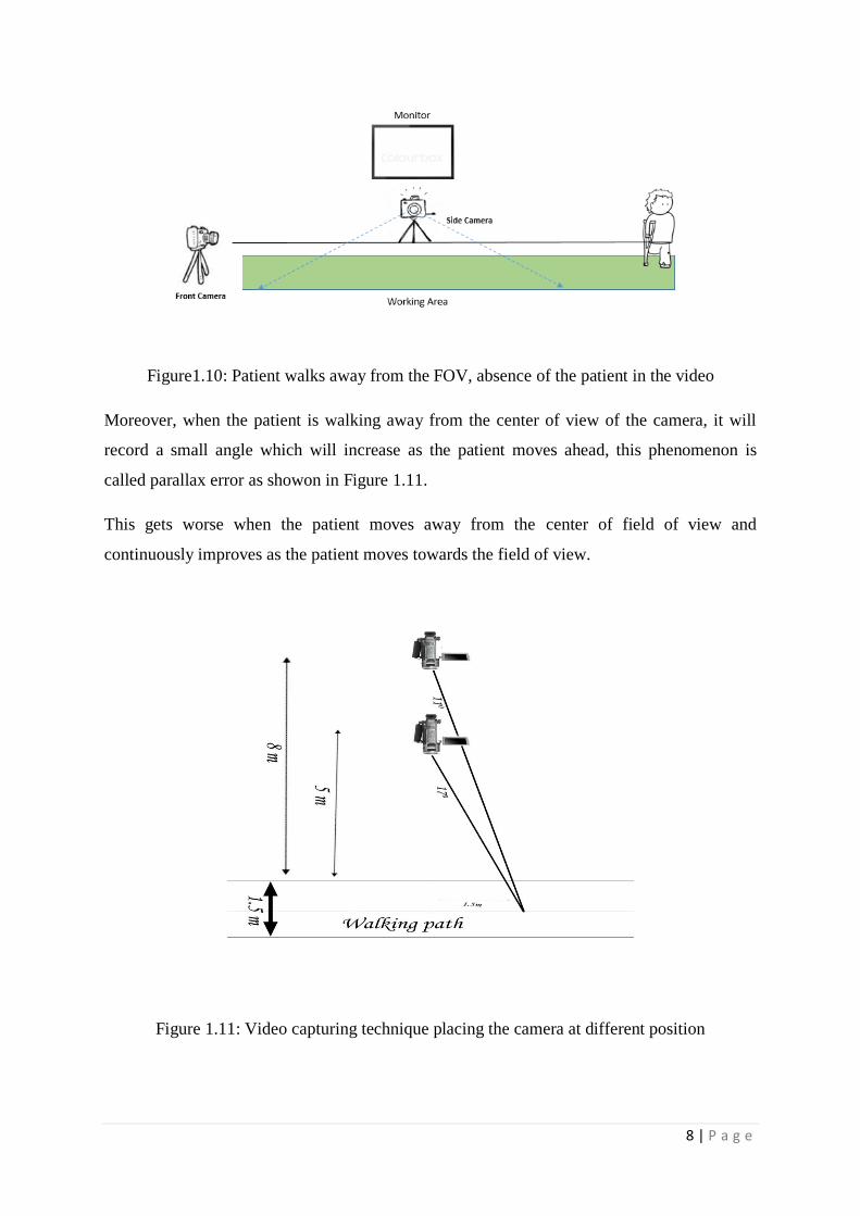
Figure1.10: Patient walks away from the FOV, absence of the patient in the video

Moreover, when the patient is walking away from the center of view of the camera, it will

record a small angle which will increase as the patient moves ahead, this phenomenon is

called parallax error as showon in Figure 1.11.

This gets worse when the patient moves away from the center of field of view and

continuously improves as the patient moves towards the field of view.

Figure 1.11: Video capturing technique placing the camera at different position

9 | P a g e

As shown in the above Figure 1.11 , if the camera is positioned further back then the parallax

error will reduce but at the same time the amount of light received by the camera will also be

reduced by square of distance, affecting the image quality. Thus, there needs to be a

compromise between reducing parallax error and keeping bright images.

If we see back to the Figure 1.7, it is clear that there is some dead space while recording

video with a fixed camera because there are parts of the sagittal plane view of the patient

which cannot be captured. It may be possible to better use these dead spaces during video

recording for gait analysis.

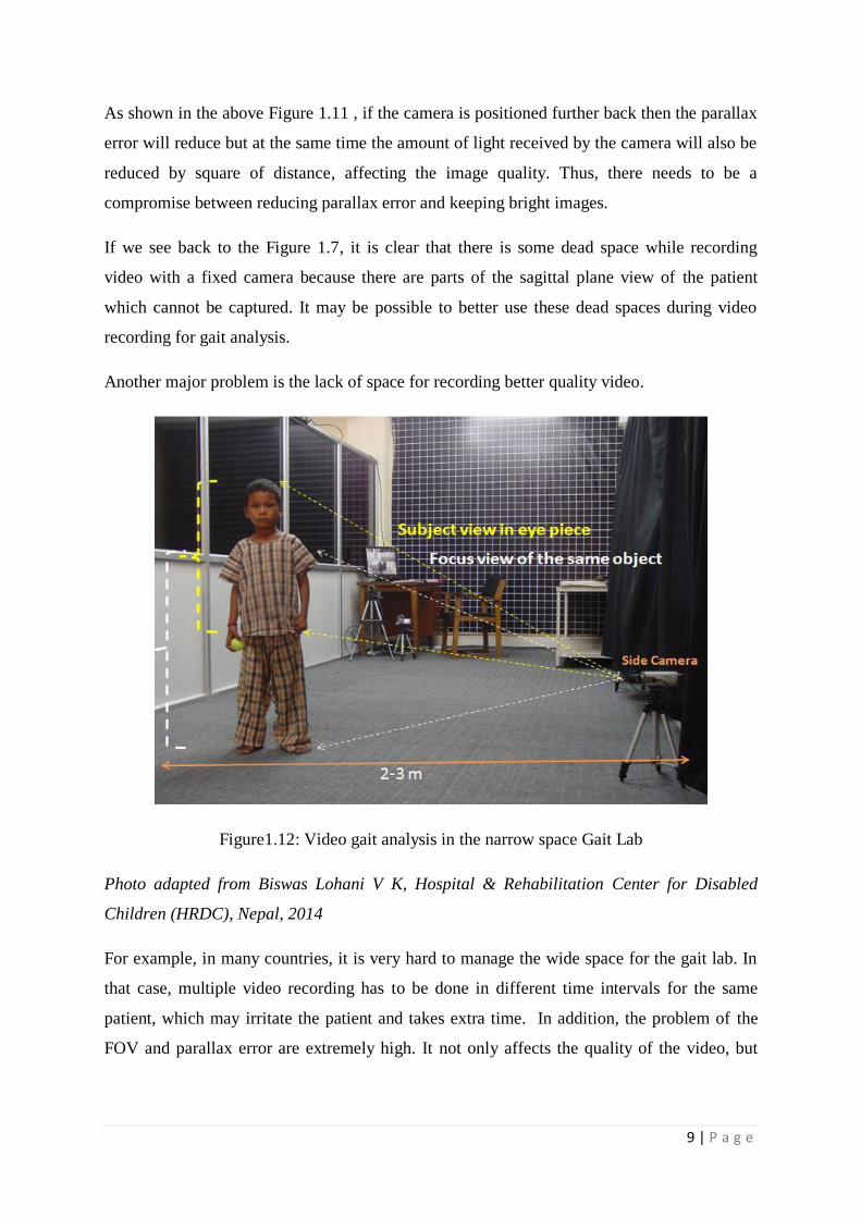
Another major problem is the lack of space for recording better quality video.

Figure1.12: Video gait analysis in the narrow space Gait Lab

Photo adapted from Biswas Lohani V K, Hospital & Rehabilitation Center for Disabled

Children (HRDC), Nepal, 2014

For example, in many countries, it is very hard to manage the wide space for the gait lab. In

that case, multiple video recording has to be done in different time intervals for the same

patient, which may irritate the patient and takes extra time. In addition, the problem of the

FOV and parallax error are extremely high. It not only affects the quality of the video, but

10 | P a g e

also gives the wrong clinical data and that's directly related to the patient so this could be the

biggest challenge in 2D video gait analysis.

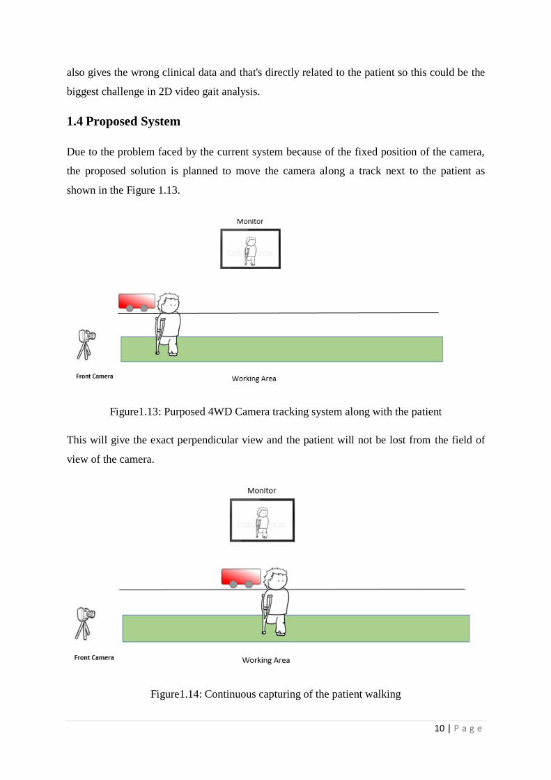
1.4 Proposed System

Due to the problem faced by the current system because of the fixed position of the camera,

the proposed solution is planned to move the camera along a track next to the patient as

shown in the Figure 1.13.

Figure1.13: Purposed 4WD Camera tracking system along with the patient

This will give the exact perpendicular view and the patient will not be lost from the field of

view of the camera.

Figure1.14: Continuous capturing of the patient walking

11 | P a g e

The loss of patients from the FOV is faced at almost all gait labs where there are still cameras

as shown in the figure.

Therefore, the proposed system will help to eliminate this problem and keep the patient

within its FOV all the time. This system can also be used in underdeveloped countries in the

narrow space gait lab as it moves along with the patient walking.

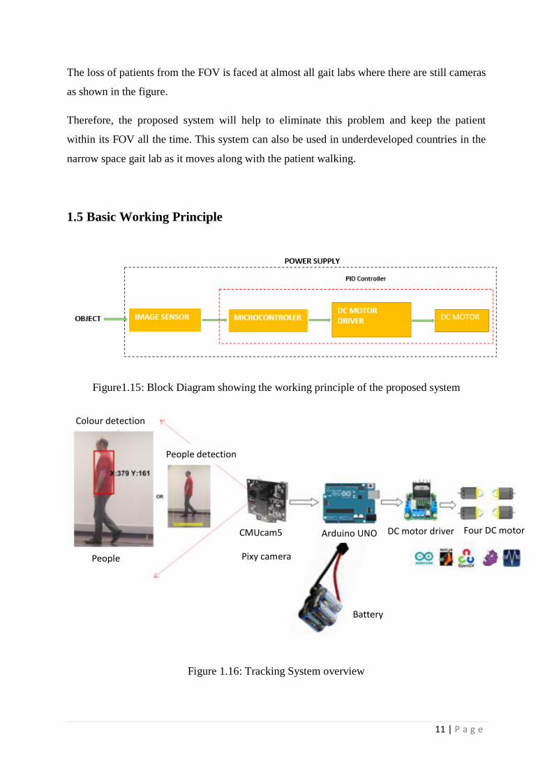
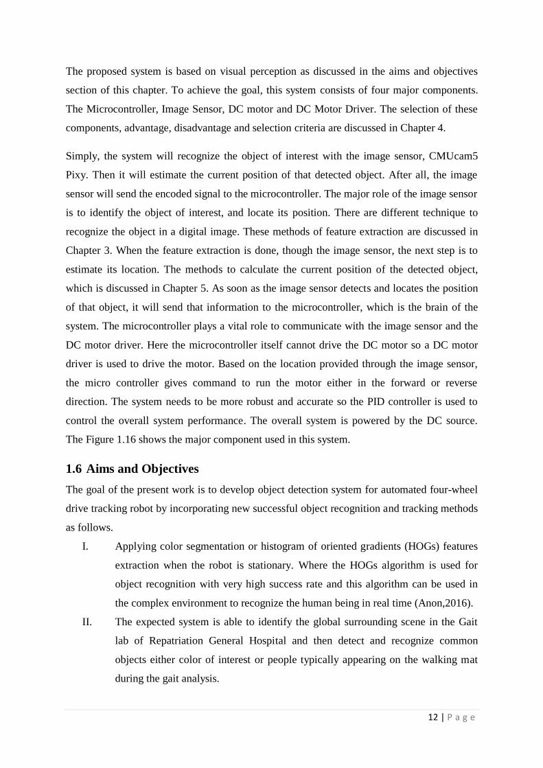
1.5 Basic Working Principle

Figure1.15: Block Diagram showing the working principle of the proposed system

Figure 1.16: Tracking System overview

Colour detection

People detection

CMUcam5

Pixy camera People

Arduino UNO DC motor driver Four DC motor

Battery

12 | P a g e

The proposed system is based on visual perception as discussed in the aims and objectives

section of this chapter. To achieve the goal, this system consists of four major components.

The Microcontroller, Image Sensor, DC motor and DC Motor Driver. The selection of these

components, advantage, disadvantage and selection criteria are discussed in Chapter 4.

Simply, the system will recognize the object of interest with the image sensor, CMUcam5

Pixy. Then it will estimate the current position of that detected object. After all, the image

sensor will send the encoded signal to the microcontroller. The major role of the image sensor

is to identify the object of interest, and locate its position. There are different technique to

recognize the object in a digital image. These methods of feature extraction are discussed in

Chapter 3. When the feature extraction is done, though the image sensor, the next step is to

estimate its location. The methods to calculate the current position of the detected object,

which is discussed in Chapter 5. As soon as the image sensor detects and locates the position

of that object, it will send that information to the microcontroller, which is the brain of the

system. The microcontroller plays a vital role to communicate with the image sensor and the

DC motor driver. Here the microcontroller itself cannot drive the DC motor so a DC motor

driver is used to drive the motor. Based on the location provided through the image sensor,

the micro controller gives command to run the motor either in the forward or reverse

direction. The system needs to be more robust and accurate so the PID controller is used to

control the overall system performance. The overall system is powered by the DC source.

The Figure 1.16 shows the major component used in this system.

1.6 Aims and Objectives

The goal of the present work is to develop object detection system for automated four-wheel

drive tracking robot by incorporating new successful object recognition and tracking methods

as follows.

I. Applying color segmentation or histogram of oriented gradients (HOGs) features

extraction when the robot is stationary. Where the HOGs algorithm is used for

object recognition with very high success rate and this algorithm can be used in

the complex environment to recognize the human being in real time (Anon,2016).

II. The expected system is able to identify the global surrounding scene in the Gait

lab of Repatriation General Hospital and then detect and recognize common

objects either color of interest or people typically appearing on the walking mat

during the gait analysis.

13 | P a g e

III. The system tracks these objects and predicts their positions in the scene if they are

temporarily disappearing.

1.7 Design Specification of the tracking device

1.7.1 Functional requirements

a. Straight and automated

The camera moves straight, tracking the patient automatically with their

motion. The necessity of the track in this case is to record the gait without any

shaking or jerking.

b. Length

The tracks of the gait lab in SA movement analysis centre are of 6 metres in

length. So the tracking unit should track the patient at least 6 metres. The lenth

of the track for camera dolly should be designed to be 6 metres length. And

the distance of camera unit from the walkway should be 4 metres.

c. Speed

Normal speed of patient is about 1.5m/s (Carey, 2005) so that the camera

trolley should be designed to be able to achieve the same speed. But, it will

also need to adjust to changes in the speed of the patient and move

accordingly.

d. Focus

The mainly purpose of the side camera recording the lateral view is to

visualize and measure the hip, knee and flexion and extension. So the focus of

the camera should be perpendicular to capture the required area. We can also

focus the camera from head to toe during the baseline walking and then with

reference to the captured video, we can change the focus during the running of

gait measurement. But it is very important to adjust the focus of camera height

and the target area and the lens should be perpendicular to the object to

measure the angles accurately.

e. Motor Operated system

The tracking unit should use the motors to drive the camera.

14 | P a g e

f. Start and stop

As soon as the system detects the object, the system should control the start

and stop so that the tracking of the object will not miss its movement during

gait measurement.

g. Manual/Automatic operated

As the system works automatically when the patient moves, it should be also

possible to move the camera unit manually during ‘’OFF’’ position.

h. Data cables and power cable management

There are different types of cables available in the market so the selection of

the data cables are well as the power cables are essential before designing the

system. As currently available data cables, fire wire cables would be great in

the system because of its high speed data transfer rate.The selection of power

cable must meet the Australian standard.

1.7.2 Design consideration

1.7.2.1 Hardware

There are different types of motion tracking system, with interfacing for synchronous

analogue and digital data acquisition (e.g. force plate, EMG). In this project, selection of the

hardware is not a part and the scope of it, but understanding of the hardware part gives the

fundamental ideas in the measurement of different component use like cameras, force plate

etc.

1.7.2.2 Co-ordinate system

The long axis of the measurement unit defines the direction of the X-axis (normally

horizontal and parallel to the walkway). The perpendicular away from the unit defines the

positive Y-axis (normally horizontal, across the walkway). The other perpendicular (vertical)

defines the Z-axis (positive up). The origin of the coordinate system is offset by the user to

any point in the field of view.

15 | P a g e

1.7.2.4 Software

The IDE Pixymon is used to extract the features of a color object. Likewise the Arduino IDE

and Matlab is used to control the system and test the result and performance.

1.7.2.5 Cost

Cost estimation is the major selection criteria in any technology before its design. We need to

minimize the costs much as we can so that the system is reliable and can be affordable in any

locality. Therefore the maximum budget for this project is $600.

16 | P a g e

CHAPTER 2 Related Work 2.1 Commercial Systems

There are different tracking systems which can be found in the market. These tracking

systems have been used for different purposes like, filming, sports, television channels,

hospitals (Gait Lab). In this chapter, some of the systems that are on the market will be

discussed.

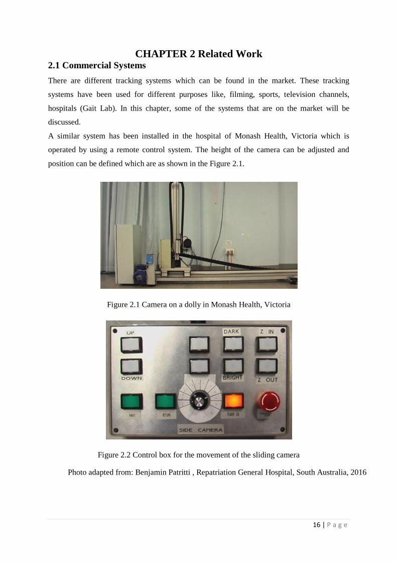
A similar system has been installed in the hospital of Monash Health, Victoria which is

operated by using a remote control system. The height of the camera can be adjusted and

position can be defined which are as shown in the Figure 2.1.

Figure 2.1 Camera on a dolly in Monash Health, Victoria

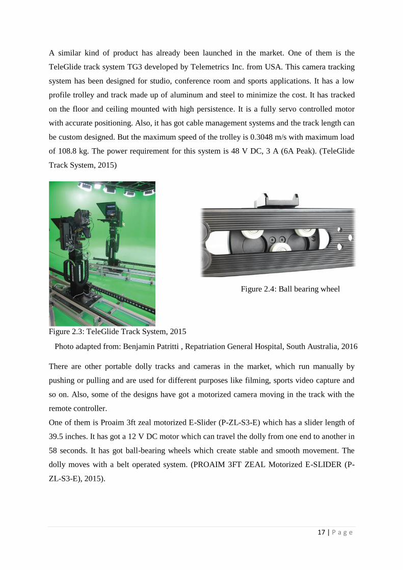
Figure 2.2 Control box for the movement of the sliding camera

Photo adapted from: Benjamin Patritti , Repatriation General Hospital, South Australia, 2016

17 | P a g e

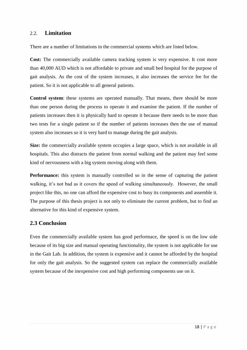
A similar kind of product has already been launched in the market. One of them is the

TeleGlide track system TG3 developed by Telemetrics Inc. from USA. This camera tracking

system has been designed for studio, conference room and sports applications. It has a low

profile trolley and track made up of aluminum and steel to minimize the cost. It has tracked

on the floor and ceiling mounted with high persistence. It is a fully servo controlled motor

with accurate positioning. Also, it has got cable management systems and the track length can

be custom designed. But the maximum speed of the trolley is 0.3048 m/s with maximum load

of 108.8 kg. The power requirement for this system is 48 V DC, 3 A (6A Peak). (TeleGlide

Track System, 2015)

Figure 2.3: TeleGlide Track System, 2015

There are other portable dolly tracks and cameras in the market, which run manually by

pushing or pulling and are used for different purposes like filming, sports video capture and

so on. Also, some of the designs have got a motorized camera moving in the track with the

remote controller.

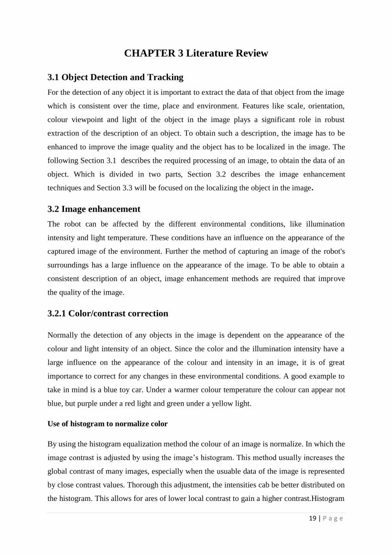
One of them is Proaim 3ft zeal motorized E-Slider (P-ZL-S3-E) which has a slider length of

39.5 inches. It has got a 12 V DC motor which can travel the dolly from one end to another in

58 seconds. It has got ball-bearing wheels which create stable and smooth movement. The

dolly moves with a belt operated system. (PROAIM 3FT ZEAL Motorized E-SLIDER (P-

ZL-S3-E), 2015).

Figure 2.4: Ball bearing wheel

slider

Photo adapted from: Benjamin Patritti , Repatriation General Hospital, South Australia, 2016

18 | P a g e

2.2. Limitation

There are a number of limitations in the commercial systems which are listed below.

Cost: The commercially available camera tracking system is very expensive. It cost more

than 40,000 AUD which is not affordable to private and small bed hospital for the purpose of

gait analysis. As the cost of the system increases, it also increases the service fee for the

patient. So it is not applicable to all general patients.

Control system: these systems are operated manually. That means, there should be more

than one person during the process to operate it and examine the patient. If the number of

patients increases then it is physically hard to operate it because there needs to be more than

two tests for a single patient so if the number of patients increases then the use of manual

system also increases so it is very hard to manage during the gait analysis.

Size: the commercially available system occupies a large space, which is not available in all

hospitals. This also distracts the patient from normal walking and the patient may feel some

kind of nervousness with a big system moving along with them.

Performance: this system is manually controlled so in the sense of capturing the patient

walking, it’s not bad as it covers the speed of walking simultaneously. However, the small

project like this, no one can afford the expensive cost to busy its components and assemble it.

The purpose of this thesis project is not only to eliminate the current problem, but to find an

alternative for this kind of expensive system.

2.3 Conclusion

Even the commercially available system has good performace, the speed is on the low side

because of its big size and manual operating functionality, the system is not applicable for use

in the Gait Lab. In addition, the system is expensive and it cannot be afforded by the hospital

for only the gait analysis. So the suggested system can replace the commercially available

system because of the inexpensive cost and high performing components use on it.

19 | P a g e

CHAPTER 3 Literature Review

3.1 Object Detection and Tracking

For the detection of any object it is important to extract the data of that object from the image

which is consistent over the time, place and environment. Features like scale, orientation,

colour viewpoint and light of the object in the image plays a significant role in robust

extraction of the description of an object. To obtain such a description, the image has to be

enhanced to improve the image quality and the object has to be localized in the image. The

following Section 3.1 describes the required processing of an image, to obtain the data of an

object. Which is divided in two parts, Section 3.2 describes the image enhancement

techniques and Section 3.3 will be focused on the localizing the object in the image.

3.2 Image enhancement

The robot can be affected by the different environmental conditions, like illumination

intensity and light temperature. These conditions have an influence on the appearance of the

captured image of the environment. Further the method of capturing an image of the robot's

surroundings has a large influence on the appearance of the image. To be able to obtain a

consistent description of an object, image enhancement methods are required that improve

the quality of the image.

3.2.1 Color/contrast correction

Normally the detection of any objects in the image is dependent on the appearance of the

colour and light intensity of an object. Since the color and the illumination intensity have a

large influence on the appearance of the colour and intensity in an image, it is of great

importance to correct for any changes in these environmental conditions. A good example to

take in mind is a blue toy car. Under a warmer colour temperature the colour can appear not

blue, but purple under a red light and green under a yellow light.

Use of histogram to normalize color

By using the histogram equalization method the colour of an image is normalize. In which the

image contrast is adjusted by using the image’s histogram. This method usually increases the

global contrast of many images, especially when the usuable data of the image is represented

by close contrast values. Thorough this adjustment, the intensities cab be better distributed on

the histogram. This allows for ares of lower local contrast to gain a higher contrast.Histogram

20 | P a g e

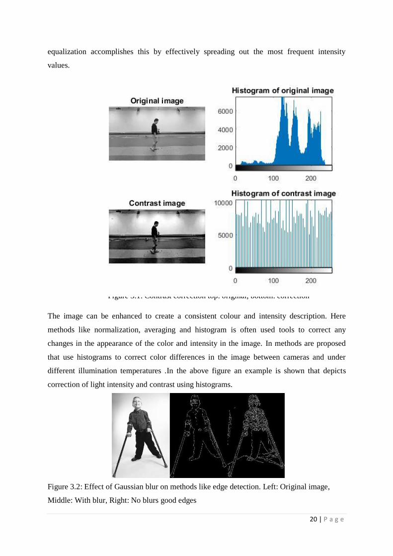
equalization accomplishes this by effectively spreading out the most frequent intensity

values.

Figure 3.1: Contrast correction top: original, bottom: correction

The image can be enhanced to create a consistent colour and intensity description. Here

methods like normalization, averaging and histogram is often used tools to correct any

changes in the appearance of the color and intensity in the image. In methods are proposed

that use histograms to correct color differences in the image between cameras and under

different illumination temperatures .In the above figure an example is shown that depicts

correction of light intensity and contrast using histograms.

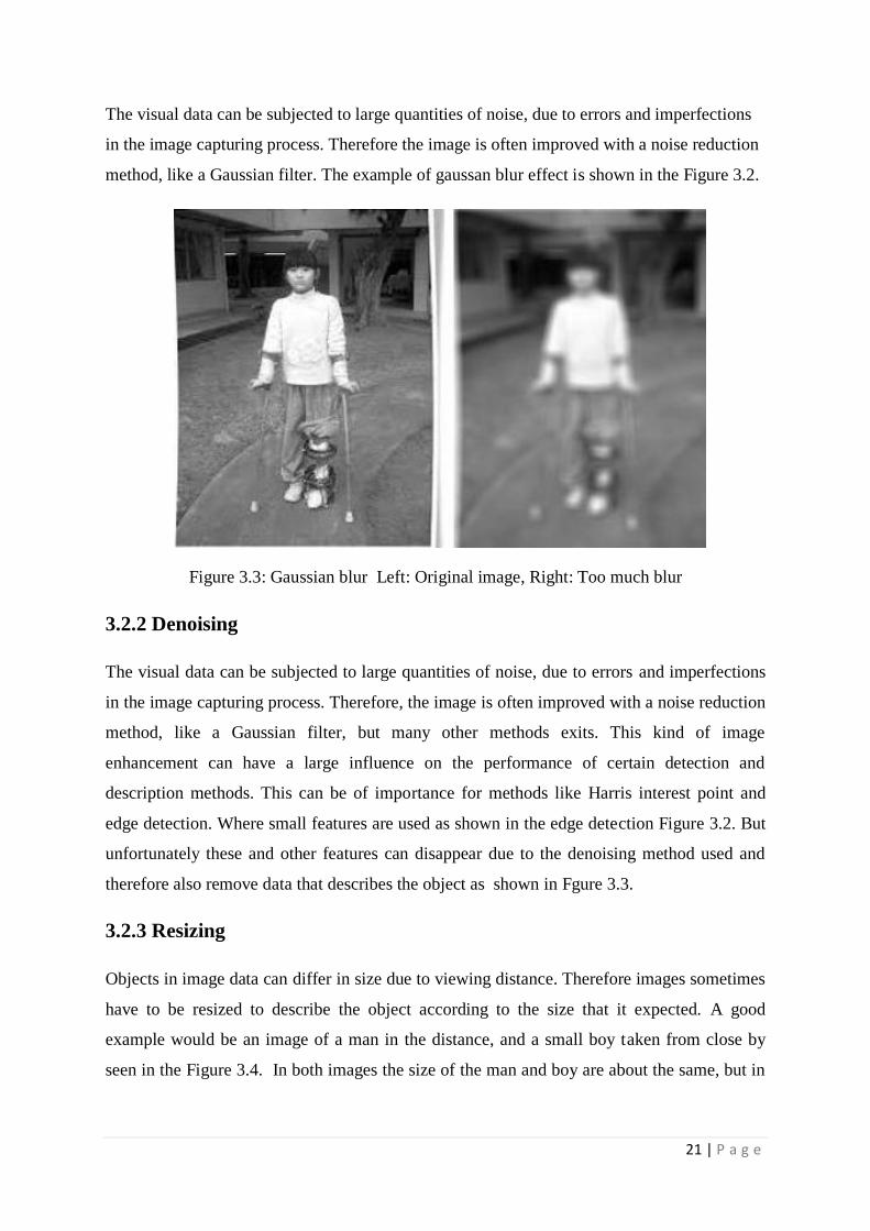
Figure 3.2: Effect of Gaussian blur on methods like edge detection. Left: Original image,

Middle: With blur, Right: No blurs good edges

21 | P a g e

The visual data can be subjected to large quantities of noise, due to errors and imperfections

in the image capturing process. Therefore the image is often improved with a noise reduction

method, like a Gaussian filter. The example of gaussan blur effect is shown in the Figure 3.2.

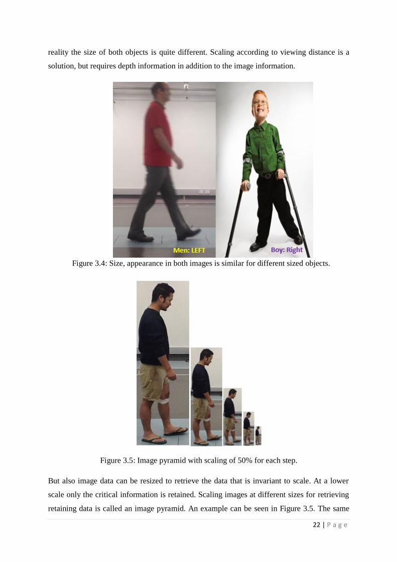
Figure 3.3: Gaussian blur Left: Original image, Right: Too much blur

3.2.2 Denoising

The visual data can be subjected to large quantities of noise, due to errors and imperfections

in the image capturing process. Therefore, the image is often improved with a noise reduction

method, like a Gaussian filter, but many other methods exits. This kind of image

enhancement can have a large influence on the performance of certain detection and

description methods. This can be of importance for methods like Harris interest point and

edge detection. Where small features are used as shown in the edge detection Figure 3.2. But

unfortunately these and other features can disappear due to the denoising method used and

therefore also remove data that describes the object as shown in Fgure 3.3.

3.2.3 Resizing

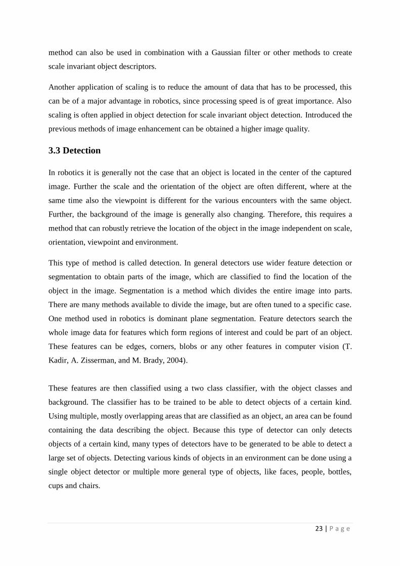
Objects in image data can differ in size due to viewing distance. Therefore images sometimes

have to be resized to describe the object according to the size that it expected. A good

example would be an image of a man in the distance, and a small boy taken from close by

seen in the Figure 3.4. In both images the size of the man and boy are about the same, but in

22 | P a g e

reality the size of both objects is quite different. Scaling according to viewing distance is a

solution, but requires depth information in addition to the image information.

Figure 3.4: Size, appearance in both images is similar for different sized objects.

Figure 3.5: Image pyramid with scaling of 50% for each step.

But also image data can be resized to retrieve the data that is invariant to scale. At a lower

scale only the critical information is retained. Scaling images at different sizes for retrieving

retaining data is called an image pyramid. An example can be seen in Figure 3.5. The same

23 | P a g e

method can also be used in combination with a Gaussian filter or other methods to create

scale invariant object descriptors.

Another application of scaling is to reduce the amount of data that has to be processed, this

can be of a major advantage in robotics, since processing speed is of great importance. Also

scaling is often applied in object detection for scale invariant object detection. Introduced the

previous methods of image enhancement can be obtained a higher image quality.

3.3 Detection

In robotics it is generally not the case that an object is located in the center of the captured

image. Further the scale and the orientation of the object are often different, where at the

same time also the viewpoint is different for the various encounters with the same object.

Further, the background of the image is generally also changing. Therefore, this requires a

method that can robustly retrieve the location of the object in the image independent on scale,

orientation, viewpoint and environment.

This type of method is called detection. In general detectors use wider feature detection or

segmentation to obtain parts of the image, which are classified to find the location of the

object in the image. Segmentation is a method which divides the entire image into parts.

There are many methods available to divide the image, but are often tuned to a specific case.

One method used in robotics is dominant plane segmentation. Feature detectors search the

whole image data for features which form regions of interest and could be part of an object.

These features can be edges, corners, blobs or any other features in computer vision (T.

Kadir, A. Zisserman, and M. Brady, 2004).

These features are then classified using a two class classifier, with the object classes and

background. The classifier has to be trained to be able to detect objects of a certain kind.

Using multiple, mostly overlapping areas that are classified as an object, an area can be found

containing the data describing the object. Because this type of detector can only detects

objects of a certain kind, many types of detectors have to be generated to be able to detect a

large set of objects. Detecting various kinds of objects in an environment can be done using a

single object detector or multiple more general type of objects, like faces, people, bottles,

cups and chairs.

24 | P a g e

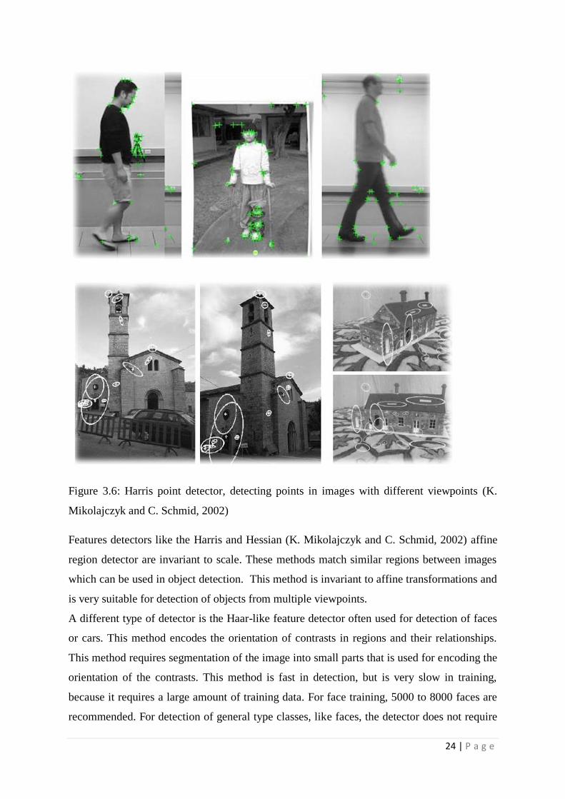
Figure 3.6: Harris point detector, detecting points in images with different viewpoints (K.

Mikolajczyk and C. Schmid, 2002)

Features detectors like the Harris and Hessian (K. Mikolajczyk and C. Schmid, 2002) affine

region detector are invariant to scale. These methods match similar regions between images

which can be used in object detection. This method is invariant to affine transformations and

is very suitable for detection of objects from multiple viewpoints.

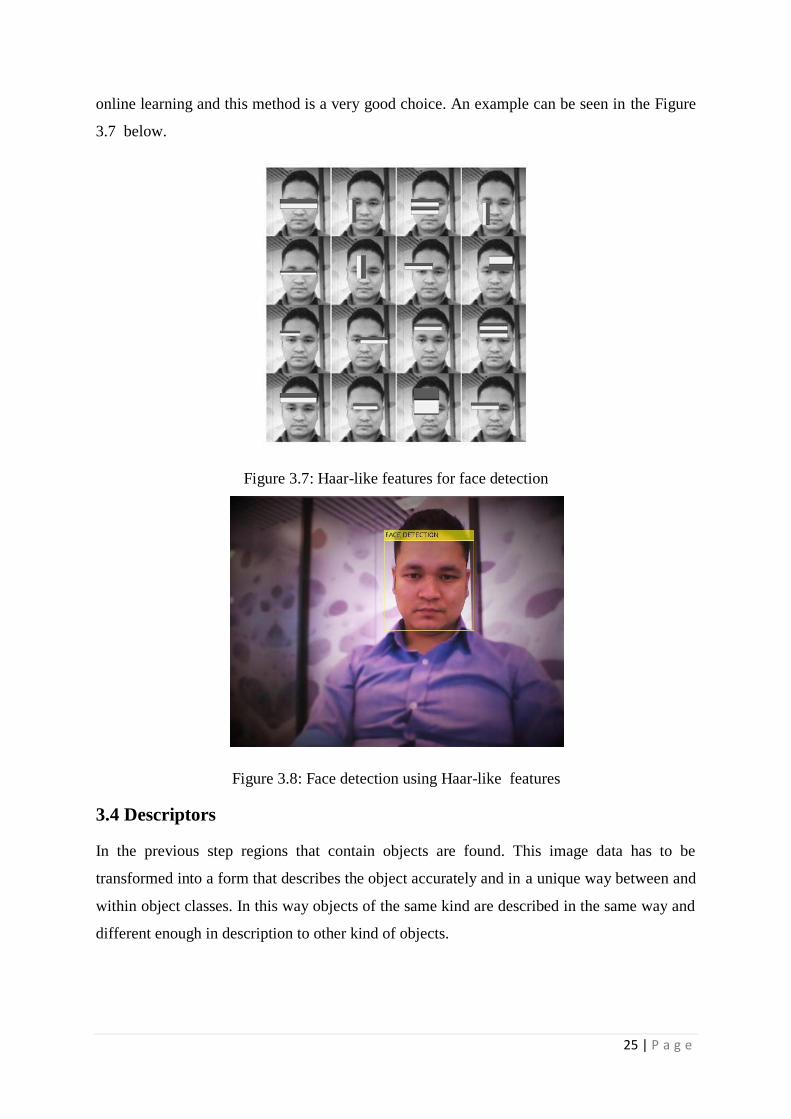
A different type of detector is the Haar-like feature detector often used for detection of faces

or cars. This method encodes the orientation of contrasts in regions and their relationships.

This method requires segmentation of the image into small parts that is used for encoding the

orientation of the contrasts. This method is fast in detection, but is very slow in training,

because it requires a large amount of training data. For face training, 5000 to 8000 faces are

recommended. For detection of general type classes, like faces, the detector does not require

25 | P a g e

online learning and this method is a very good choice. An example can be seen in the Figure

3.7 below.

Figure 3.7: Haar-like features for face detection

Figure 3.8: Face detection using Haar-like features

3.4 Descriptors

In the previous step regions that contain objects are found. This image data has to be

transformed into a form that describes the object accurately and in a unique way between and

within object classes. In this way objects of the same kind are described in the same way and

different enough in description to other kind of objects.

26 | P a g e

Descriptor methods can describe the object in different ways like, its red or it is cube shaped

but there are a lot of objects that are red and cube shaped. So a single unique description or a

combination of descriptions should be found to uniquely and accurately describe the object.

These descriptions should also be invariant to environmental conditions.

For example, a human tracking robot . It is important to find a way to describe the human that

is unique for the human only and is not used for other kind of objects. In this case the

function of an object makes it a human. It is rather difficult to derive the function of an object

solely by its appearance, there is no color, texture or shape that is solely used for objects.

Therefore a way has to be found that can be used to classify an object as a human.

To find the features of object, different method use various combinations of descriptions, like

object features, context and interactions to determine the function of an object. These are

based on the experience of previous observations of objects and on observations of the

current situation. Therefore, this Section 3.4.1 of the literature review is focused on what

combination of visual recognition methods can be used to determine the function and

interaction of an object. Once the object is detected, automated tracking robots can work

effectively.

Following are the some of the description methods that have been tested during the literature

reviews.

3.4.1 Color descriptor

The color of an object can be used to describe the object. This has advantages that it is simple

and fast, but also its disadvantages because it is dependent on the light. Converting the color

to for example, HSV color spaces can help to achieve illuminate invariant description, but

there are more similar colour spaces. Here the colour is described with hue, saturation and

value. The hue described the colour, saturation, how much colour is used and value the

illumination intensity. So when the light intensity changes the hue does not change and if the

colour of the light changes the saturation stays the same.

For robotics, a colour descriptor can be very useful, since it is fast and if combined with other

descriptors it can provide a robust description of the object. Changes in color due to

illumination changes can be corrected by the colour enhancement methods. There are

different colour enhanancement techniques like gamma correction, contrast stretching,

27 | P a g e

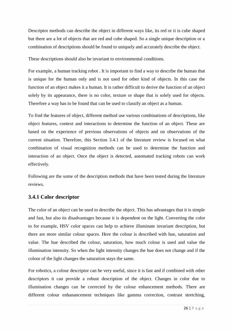
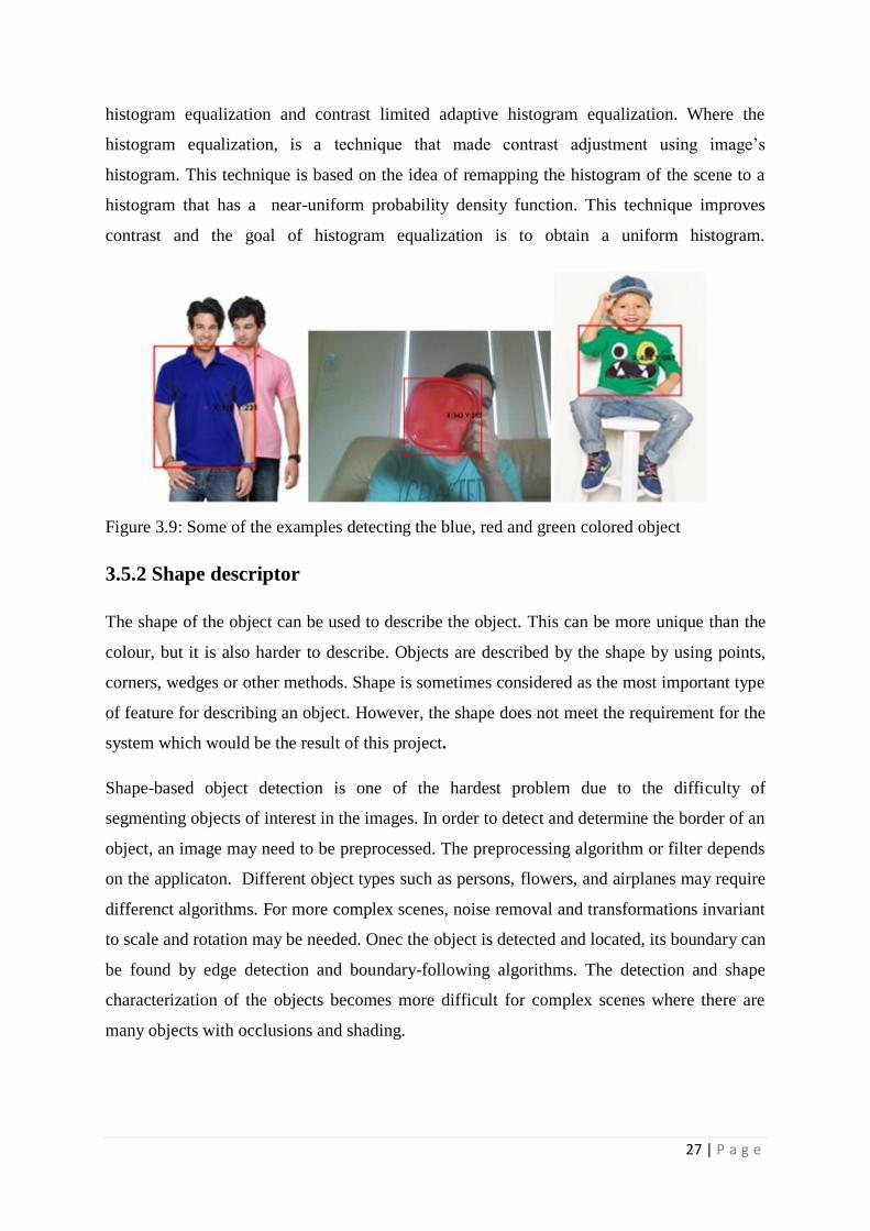
histogram equalization and contrast limited adaptive histogram equalization. Where the

histogram equalization, is a technique that made contrast adjustment using image’s

histogram. This technique is based on the idea of remapping the histogram of the scene to a

histogram that has a near-uniform probability density function. This technique improves

contrast and the goal of histogram equalization is to obtain a uniform histogram.

Figure 3.9: Some of the examples detecting the blue, red and green colored object

3.5.2 Shape descriptor

The shape of the object can be used to describe the object. This can be more unique than the

colour, but it is also harder to describe. Objects are described by the shape by using points,

corners, wedges or other methods. Shape is sometimes considered as the most important type

of feature for describing an object. However, the shape does not meet the requirement for the

system which would be the result of this project.

Shape-based object detection is one of the hardest problem due to the difficulty of

segmenting objects of interest in the images. In order to detect and determine the border of an

object, an image may need to be preprocessed. The preprocessing algorithm or filter depends

on the applicaton. Different object types such as persons, flowers, and airplanes may require

differenct algorithms. For more complex scenes, noise removal and transformations invariant

to scale and rotation may be needed. Onec the object is detected and located, its boundary can

be found by edge detection and boundary-following algorithms. The detection and shape

characterization of the objects becomes more difficult for complex scenes where there are

many objects with occlusions and shading.

28 | P a g e

3.5 Edge features descriptor

The shape of an object is often described by edges which within the object, but also by the

edge described by the outlines of the object. Therefore edge detection is often used in the

description of the shape. In images edges are detected and combined into continuous edges,

called pair of adjacent segments (PAS) features. These PAS features are combined into

shapes which are compared with shape models of objects. This appeared to be a good

performing application of edge detection in a shape descriptor. One of the major problems in

shape description is still the viewpoint and scale variances.

This method can be used to create a descriptor for describing the basic shape of objects. Like

the cube shape of wooden blocks or cylindrical shapes of a mug or a bottle, which could be a

good basis for describing objects. This would also be a great description method that could be

used for object detection.

3.5.1 Size descriptor

The size of an object can be used for describing an object. This is a good descriptor for

detecting objects. For example, in a person detector using HOG features, the size of the

detected human has a certain range. This means that the described area can be rejected if the

size does not fit the model. Since the size of the object is heavily dependent on how the

image is captured, depth information or comparison with other objects has to be used.

3.5.2 Shape descriptor for robots

The previously introduced shape descriptors can all be applied in robotics with some

limitations. Humans distinguish objects quite well on shape. Take for example the case in

mind where you get a present and based on the shape you feel through the wrapping paper

what the present is, like a book. But unfortunately there does not exist a method yet, that can

describe the shape of an object as robustly as humans do.

3.6 Local descriptors

Local descriptors are a class of descriptors that describes the features based on local

properties of objects rather than global properties of the object. These are commonly used

and often describe the object quite well. There are different methods to describe the local

features of an object in an image which are explained in the next section.

29 | P a g e

3.6.1 Scale- Invariant Feature Transforms (SIFTs)

This is quite suitable for object detection. It can describe the features invariant to scale and

affine transformations up to a 40 degree viewpoint angle. It uses a four step method; first

interest points that are invariant to scale and orientation are found using a difference-of-

Gaussian (DoG) methods. Next, for each interest point, a model is fited to determine scale

and location and stable key points are selected. Based on the local gradient direction for each

key point, orientations are assigned. Now the area around each key point is described with

local gradients for the selected scale. This makes the description invariant to scale,

orientation, significant shape distortions and change in illumination. Using an invariant point

detector like Harris- Laplace could improve the performance of SIFTs (Yi, Hong and Hong,

2012).

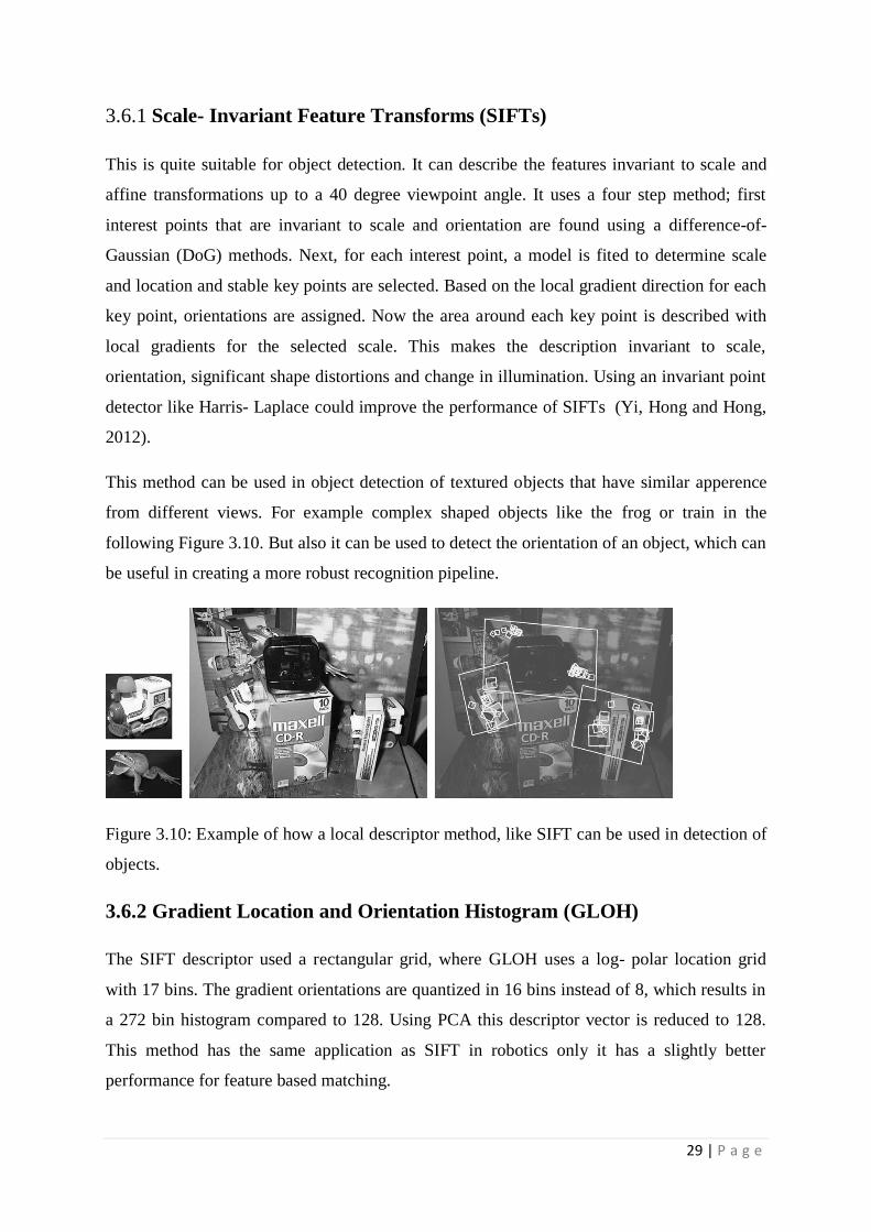
This method can be used in object detection of textured objects that have similar apperence

from different views. For example complex shaped objects like the frog or train in the

following Figure 3.10. But also it can be used to detect the orientation of an object, which can

be useful in creating a more robust recognition pipeline.

Figure 3.10: Example of how a local descriptor method, like SIFT can be used in detection of

objects.

3.6.2 Gradient Location and Orientation Histogram (GLOH)

The SIFT descriptor used a rectangular grid, where GLOH uses a log- polar location grid

with 17 bins. The gradient orientations are quantized in 16 bins instead of 8, which results in

a 272 bin histogram compared to 128. Using PCA this descriptor vector is reduced to 128.

This method has the same application as SIFT in robotics only it has a slightly better

performance for feature based matching.

30 | P a g e

3.6.3 Speeded Up Robust Features (SURFs)

SURF is an improved SIFT method. It uses a Fast- Hessian detector as interest points. At

SIFT image pyramids have to be made for different scales. SURF and SIFT both uses a

scalable filter however the difference is SIFT uses a box filter whereas SURF uses Gaussian

for detection of multiple scales. Next two Haar wavelet filters are used to determine the

orientation. Then a square region is created around the interest point in the previous retrieved

orientation. This area is divided into smaller regions and is described using the same local

gradients. The major advantages of SURF over SIFT is that it is faster in the calculation. This

makes preferable over SIFT for object detection and its applications in robotics.

3.6.4 Histogram of Oriented Gradients (HOGs)

This is a description method where for every point or region the orientation of the gradient is

used to describe that area.

The image is divided into non-overlapping 8x8 pixels patches called cells, where gradients

are calculated for each pixel. A histogram of the gradient orientations with 9 bins is generated

for each cell. This histogram is then normalized by its neighboring cells to increase

robustness to tecture and illumination variation. For each cell, the normalization is performed

across blocks of 2x2 cells resulting in a final 36- dimension feature.

Multi-scale detection is done by training one SVM classifier that has the size of the detection

window. An image pyramid is generated, which is composed of multiple scaled versions of

each frame. All image pyramid levels are then processed by the same SVM classifier.

This method can also be used for gesture and pose recognition. The application of this

method for robotics will be in the field of describing complex and deformable shapes like

persons. Detection of person is of great importance to learn from observation.

3.7 Conclusion

In this section various object feature detection methods are discussed. These methods can be

used for various proposed depending on project priority for example shape, colour pattern

etc. However, in this project the colour detection and histogram of oriented gradients (HOGs)

methods are selected becaue the colour detection and tracking methods are time efficient and

it can provide a robust description of the object where as the histrogram of oriented gradients

31 | P a g e

features are more accurate in comparision with the SIFT, SURF and other edge features

descriptors. This method is also not affected by the light due to the local orientation of the

gradient features of an object.

31 | P a g e

CHAPTER 4 Fundamentals of Robotics

4.1 Introduciton

This chapter gives an overview of the electronic component , mechanical structure and

software development used in the automated camera tracking system. The main purpose of

this project is to eliminate the current problem as mentioned in Chapter 1 with the

implementing of obejct deteciton and tracking method in image processing. Therefore, to

utilize the time as well as limited cost in an appropriate way, the required electronic and

mechnical parts are directly purchased from a trusted company based on their high data

processin rate, its accuracy on obtaining data and those which are costly affordable.

In the first part of the project, the design of the robotic platform is essential to move the robot

in a smooth linear motion and that would also help to select further electronic components

based on its size and bearing capacity.

In the second part, electronic circuit desigin is required, which can be divided into the

following sections.

a. Selection of microcontroller board

b. Selection of the image sensor

c. Selection of the motor control unit and

d. The selection of actuators

e. Selection of the power supply

After designing of the electronics part, software or coding is needed for the system to work.

Software design or algorithm development consists of

i. Matlab coding for object detection and tracking

ii. Data extraction from the image sensor

iii. Generate pulse width modulation using the microcontroller

So this chapter chapter is more focused on all the required specification to design the system

which are mentioned as the scope of this project.

32 | P a g e

4.1.1 Parts of Robotcs

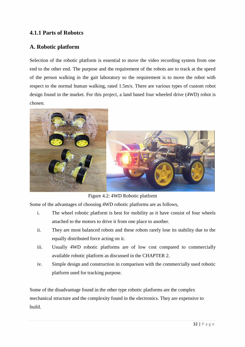
A. Robotic platform

Selection of the robotic platform is essential to move the video recording system from one

end to the other end. The purpose and the requirement of the robots are to track at the speed

of the person walking in the gait laboratory so the requirement is to move the robot with

respect to the normal human walking, rated 1.5m/s. There are various types of custom robot

design found in the market. For this project, a land based four wheeled drive (4WD) robot is

chosen.

Figure 4.2: 4WD Robotic platform

Some of the advantages of choosing 4WD robotic platforms are as follows,

i. The wheel robotic platform is best for mobility as it have consist of four wheels

attached to the motors to drive it from one place to another.

ii. They are most balanced robots and these robots rarely lose its stability due to the

equally distributed force acting on it.

iii. Usually 4WD robotic platforms are of low cost compared to commercially

available robotic platform as discussed in the CHAPTER 2.

iv. Simple design and construction in comparison with the commercially used robotic

platform used for tracking purpose.

Some of the disadvantage found in the other type robotic platforms are the complex

mechanical structure and the complexity found in the electronics. They are expensive to

build.

33 | P a g e

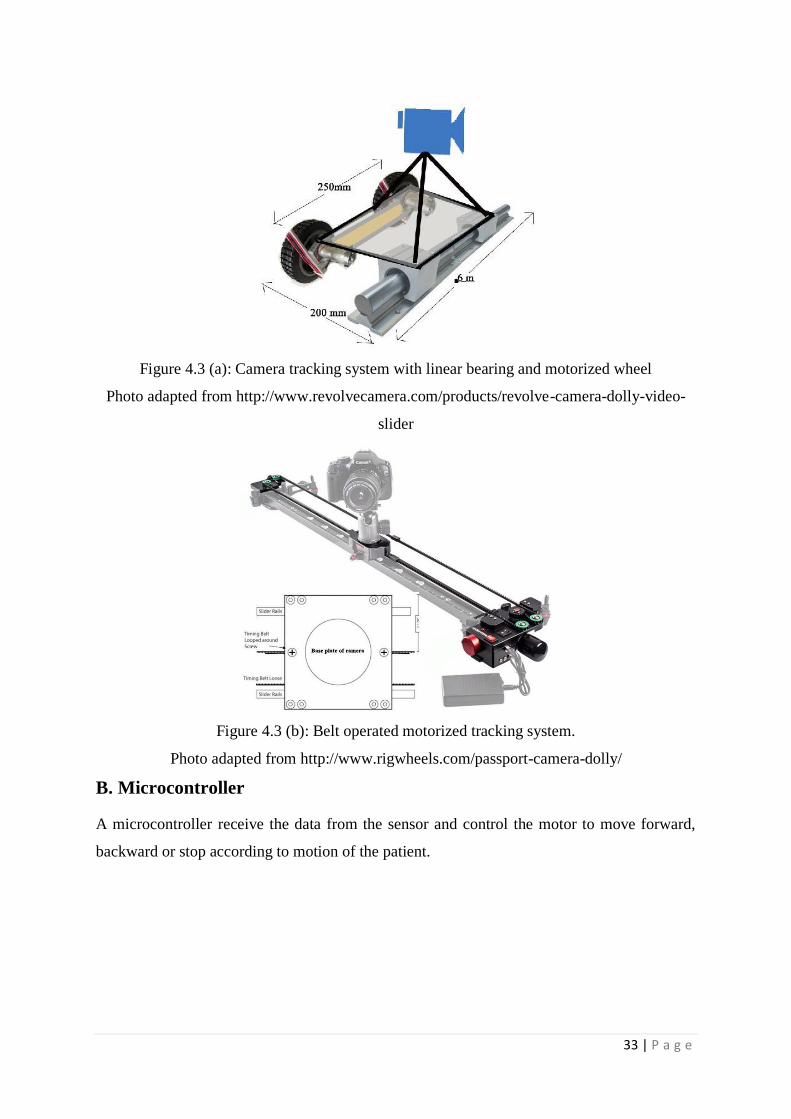
Figure 4.3 (a): Camera tracking system with linear bearing and motorized wheel

Photo adapted from http://www.revolvecamera.com/products/revolve-camera-dolly-video-

slider

Figure 4.3 (b): Belt operated motorized tracking system.

Photo adapted from http://www.rigwheels.com/passport-camera-dolly/

B. Microcontroller

A microcontroller receive the data from the sensor and control the motor to move forward,

backward or stop according to motion of the patient.

34 | P a g e

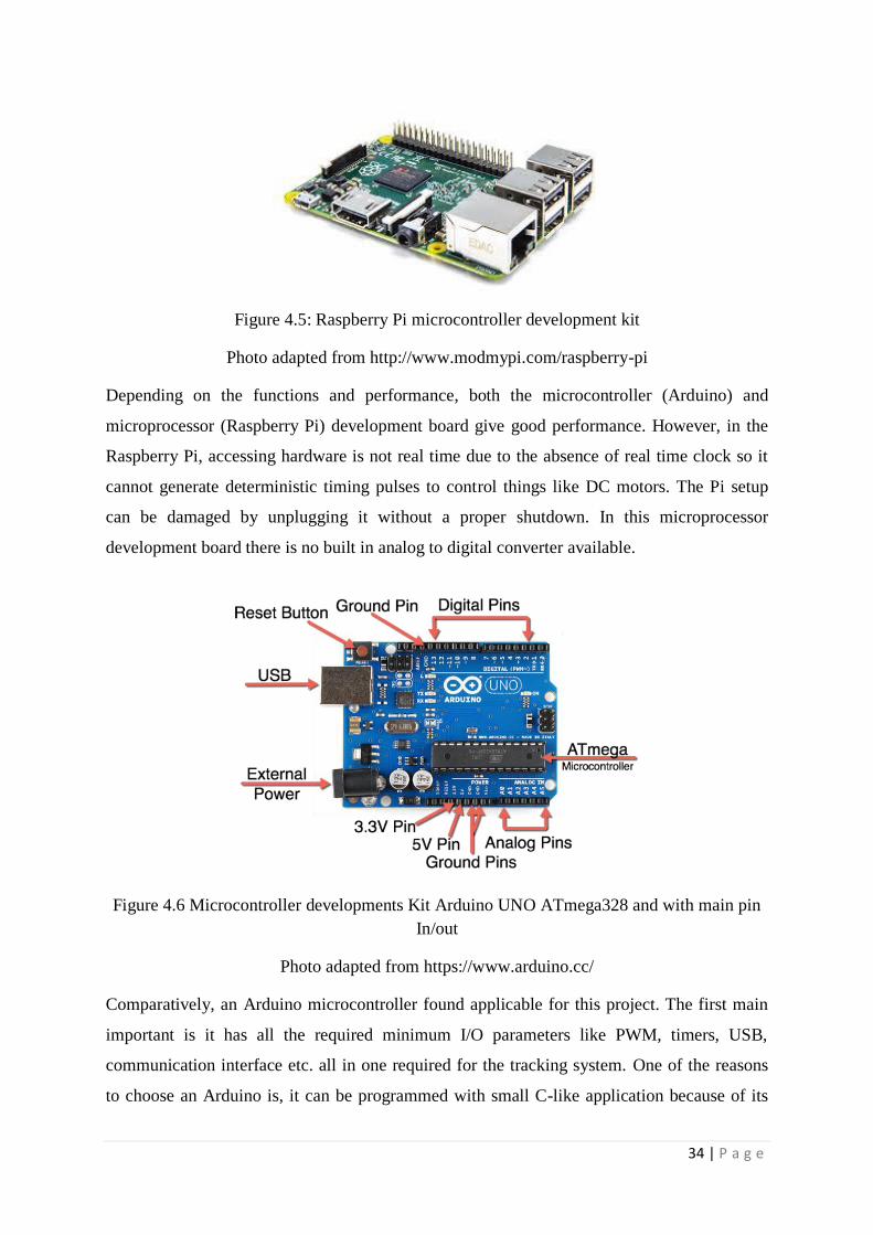
Figure 4.5: Raspberry Pi microcontroller development kit

Photo adapted from http://www.modmypi.com/raspberry-pi

Depending on the functions and performance, both the microcontroller (Arduino) and

microprocessor (Raspberry Pi) development board give good performance. However, in the

Raspberry Pi, accessing hardware is not real time due to the absence of real time clock so it

cannot generate deterministic timing pulses to control things like DC motors. The Pi setup

can be damaged by unplugging it without a proper shutdown. In this microprocessor

development board there is no built in analog to digital converter available.

Figure 4.6 Microcontroller developments Kit Arduino UNO ATmega328 and with main pin

In/out

Photo adapted from https://www.arduino.cc/

Comparatively, an Arduino microcontroller found applicable for this project. The first main

important is it has all the required minimum I/O parameters like PWM, timers, USB,

communication interface etc. all in one required for the tracking system. One of the reasons

to choose an Arduino is, it can be programmed with small C-like application because of its

35 | P a g e

simplicity. It is much better for a pure hardware project for real time application due to the

presence of a real time clock. It does only a single process at one time so can be turned on

and off when not using it. It is harder to break or damage, mean there is not any power issues

on sudden power interruption. It requires minimal setup time, and this development kit is best

for motor driving, sensor reading and led driving etc.

C. Image Sensor

The main task in this project is object detection and tracking in multiple images taken by the

image sensor. There are different image sensors found in different sources which are

compatible with the Arduino UNO microcontroller development board. Some of the most

used image sensors or camera modules are the DVS128, eDVS, OV7076 and CMUcam5

Pixy camera.

Figure 4.7: DVS128 and eDVS image sensor

Photo adapted from http://inilabs.com/products/dynamic-vision-sensors/

These image sensors are used for investigation and object detection purpose in image

processing. The embedded image sensor like DVS128 and eDVS are expensive and the

power consumption is higher than OV7670 and Pixy Camera. The main disadvantage of this

type camera is the external memory needed for data acquisition.

Figure 4.8: OV7670 Image sensor

36 | P a g e

Photo adapted from http://www.gindart.com/vga-ov7670-cmos-camera-module-lens-cmos-

640x480-sccb-compatible-w-i2c-interface-p-46577.html

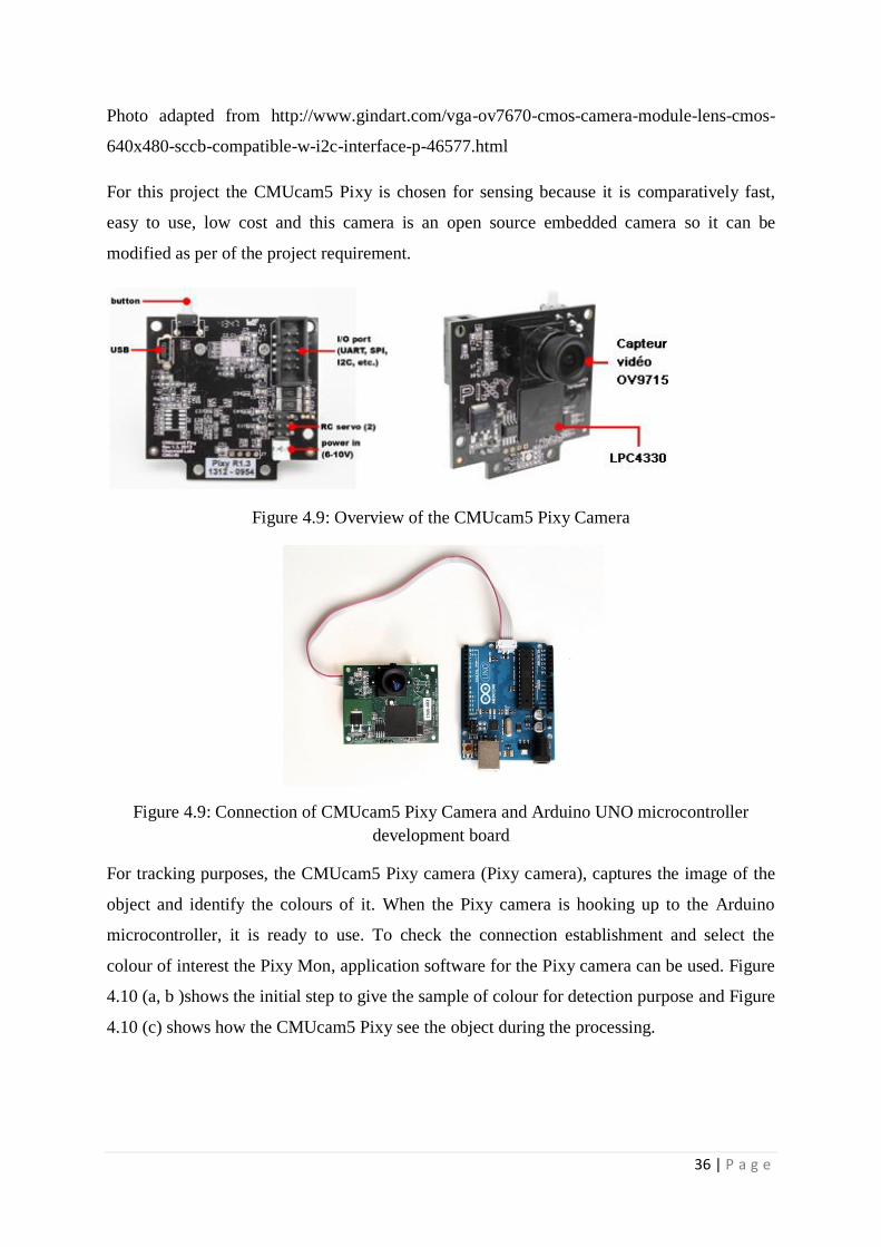
For this project the CMUcam5 Pixy is chosen for sensing because it is comparatively fast,

easy to use, low cost and this camera is an open source embedded camera so it can be

modified as per of the project requirement.

Figure 4.9: Overview of the CMUcam5 Pixy Camera

Figure 4.9: Connection of CMUcam5 Pixy Camera and Arduino UNO microcontroller

development board

For tracking purposes, the CMUcam5 Pixy camera (Pixy camera), captures the image of the

object and identify the colours of it. When the Pixy camera is hooking up to the Arduino

microcontroller, it is ready to use. To check the connection establishment and select the

colour of interest the Pixy Mon, application software for the Pixy camera can be used. Figure

4.10 (a, b )shows the initial step to give the sample of colour for detection purpose and Figure

4.10 (c) shows how the CMUcam5 Pixy see the object during the processing.

37 | P a g e

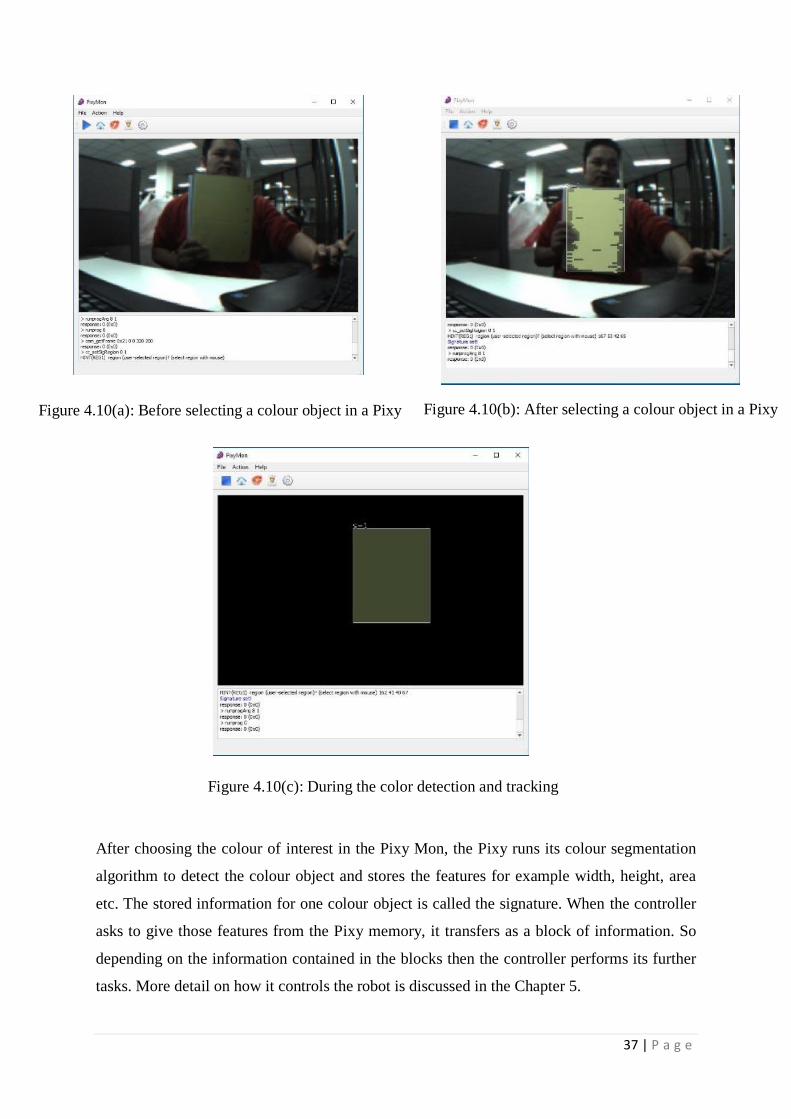
After choosing the colour of interest in the Pixy Mon, the Pixy runs its colour segmentation

algorithm to detect the colour object and stores the features for example width, height, area

etc. The stored information for one colour object is called the signature. When the controller

asks to give those features from the Pixy memory, it transfers as a block of information. So

depending on the information contained in the blocks then the controller performs its further

tasks. More detail on how it controls the robot is discussed in the Chapter 5.

Figure 4.10(a): Before selecting a colour object in a Pixy

mon

Figure 4.10(b): After selecting a colour object in a Pixy

mon

Figure 4.10(c): During the color detection and tracking

process selecting a colour object in a Pixy mon

38 | P a g e

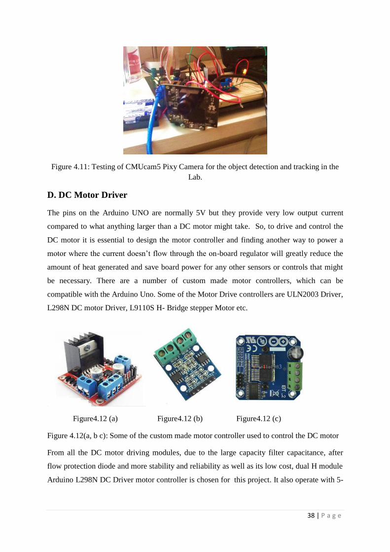
Figure 4.11: Testing of CMUcam5 Pixy Camera for the object detection and tracking in the

Lab.

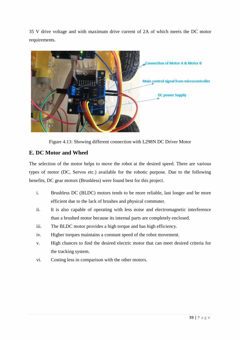
D. DC Motor Driver

The pins on the Arduino UNO are normally 5V but they provide very low output current

compared to what anything larger than a DC motor might take. So, to drive and control the

DC motor it is essential to design the motor controller and finding another way to power a

motor where the current doesn’t flow through the on-board regulator will greatly reduce the

amount of heat generated and save board power for any other sensors or controls that might

be necessary. There are a number of custom made motor controllers, which can be

compatible with the Arduino Uno. Some of the Motor Drive controllers are ULN2003 Driver,

L298N DC motor Driver, L9110S H- Bridge stepper Motor etc.

Figure4.12 (a) Figure4.12 (b) Figure4.12 (c)

Figure 4.12(a, b c): Some of the custom made motor controller used to control the DC motor

From all the DC motor driving modules, due to the large capacity filter capacitance, after

flow protection diode and more stability and reliability as well as its low cost, dual H module

Arduino L298N DC Driver motor controller is chosen for this project. It also operate with 5-

39 | P a g e

35 V drive voltage and with maximum drive current of 2A of which meets the DC motor

requirements.

Figure 4.13: Showing different connection with L298N DC Driver Motor

E. DC Motor and Wheel

The selection of the motor helps to move the robot at the desired speed. There are various

types of motor (DC, Servos etc.) available for the robotic purpose. Due to the following

benefits, DC gear motors (Brushless) were found best for this project.

i. Brushless DC (BLDC) motors tends to be more reliable, last longer and be more

efficient due to the lack of brushes and physical commuter.

ii. It is also capable of operating with less noise and electromagnetic interference

than a brushed motor because its internal parts are completely enclosed.

iii. The BLDC motor provides a high torque and has high efficiency.

iv. Higher torques maintains a constant speed of the robot movement.

v. High chances to find the desired electric motor that can meet desired criteria for

the tracking system.

vi. Costing less in comparison with the other motors.

40 | P a g e

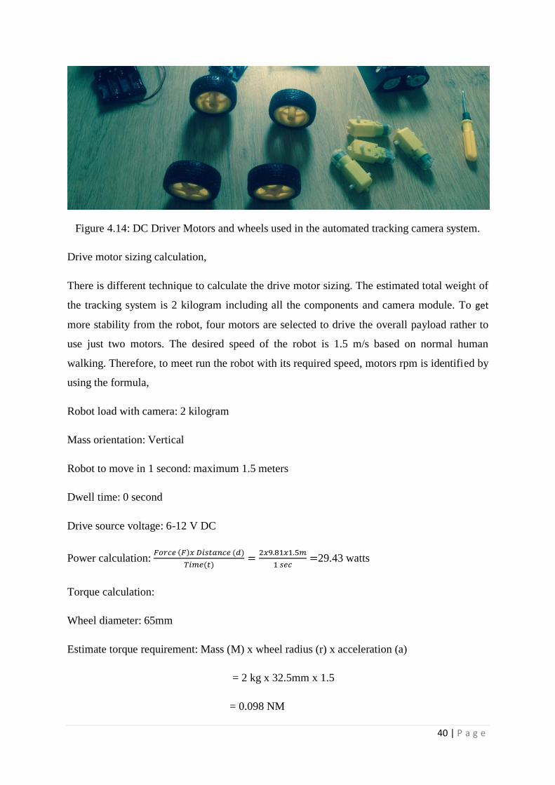
Figure 4.14: DC Driver Motors and wheels used in the automated tracking camera system.

Drive motor sizing calculation,

There is different technique to calculate the drive motor sizing. The estimated total weight of

the tracking system is 2 kilogram including all the components and camera module. To get

more stability from the robot, four motors are selected to drive the overall payload rather to

use just two motors. The desired speed of the robot is 1.5 m/s based on normal human

walking. Therefore, to meet run the robot with its required speed, motors rpm is identified by

using the formula,

Robot load with camera: 2 kilogram

Mass orientation: Vertical

Robot to move in 1 second: maximum 1.5 meters

Dwell time: 0 second

Drive source voltage: 6-12 V DC

Power calculation:

29.43 watts

Torque calculation:

Wheel diameter: 65mm

Estimate torque requirement: Mass (M) x wheel radius (r) x acceleration (a)

= 2 kg x 32.5mm x 1.5

= 0.098 NM

41 | P a g e

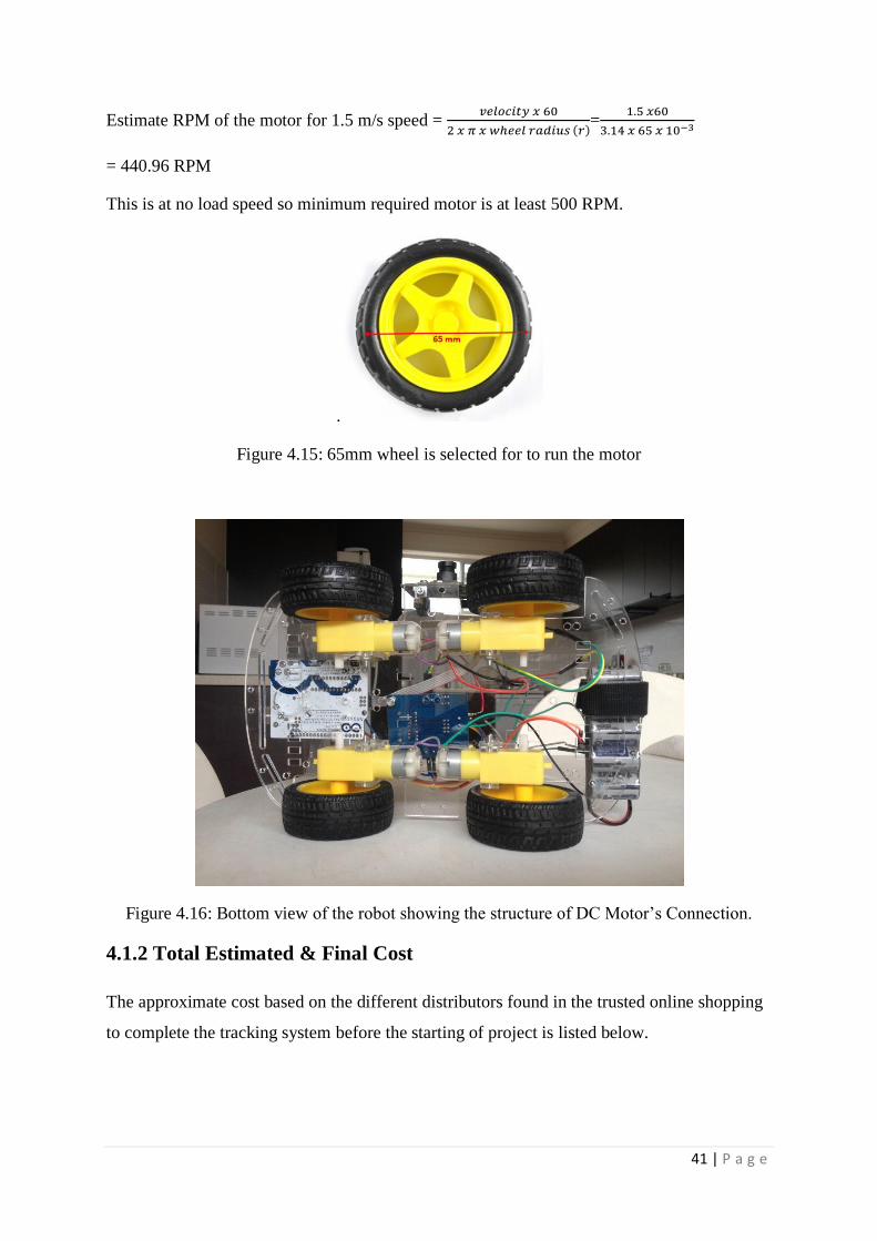
Estimate RPM of the motor for 1.5 m/s speed =

=

= 440.96 RPM

This is at no load speed so minimum required motor is at least 500 RPM.

.

Figure 4.15: 65mm wheel is selected for to run the motor

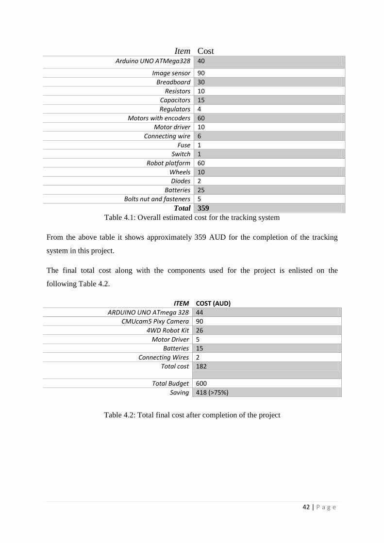
Figure 4.16: Bottom view of the robot showing the structure of DC Motor’s Connection.

4.1.2 Total Estimated & Final Cost

The approximate cost based on the different distributors found in the trusted online shopping

to complete the tracking system before the starting of project is listed below.

42 | P a g e

Item Cost Arduino UNO ATMega328 40

Image sensor 90

Breadboard 30

Resistors 10

Capacitors 15

Regulators 4

Motors with encoders 60

Motor driver 10

Connecting wire 6

Fuse 1

Switch 1

Robot platform 60

Wheels 10

Diodes 2

Batteries 25

Bolts nut and fasteners 5

Total 359

Table 4.1: Overall estimated cost for the tracking system

From the above table it shows approximately 359 AUD for the completion of the tracking

system in this project.

The final total cost along with the components used for the project is enlisted on the

following Table 4.2.

ITEM COST (AUD)

ARDUINO UNO ATmega 328 44

CMUcam5 Pixy Camera 90

4WD Robot Kit 26

Motor Driver 5

Batteries 15

Connecting Wires 2

Total cost 182

Total Budget 600

Saving 418 (>75%)

Table 4.2: Total final cost after completion of the project

43 | P a g e

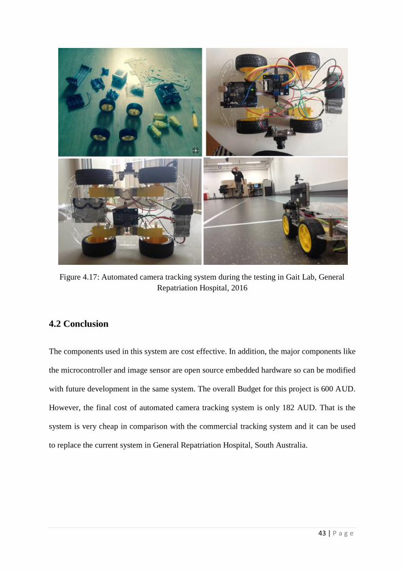
Figure 4.17: Automated camera tracking system during the testing in Gait Lab, General

Repatriation Hospital, 2016

4.2 Conclusion

The components used in this system are cost effective. In addition, the major components like

the microcontroller and image sensor are open source embedded hardware so can be modified

with future development in the same system. The overall Budget for this project is 600 AUD.

However, the final cost of automated camera tracking system is only 182 AUD. That is the

system is very cheap in comparison with the commercial tracking system and it can be used

to replace the current system in General Repatriation Hospital, South Australia.

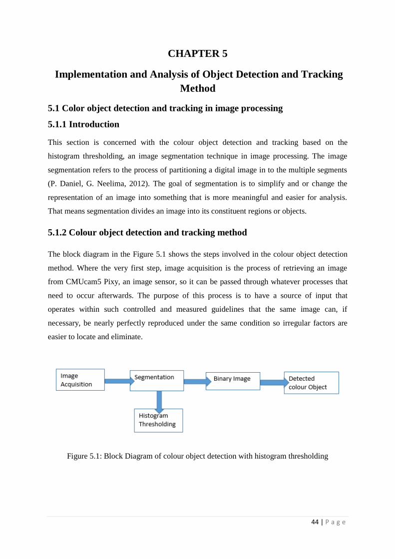
44 | P a g e

CHAPTER 5

Implementation and Analysis of Object Detection and Tracking

Method

5.1 Color object detection and tracking in image processing

5.1.1 Introduction

This section is concerned with the colour object detection and tracking based on the

histogram thresholding, an image segmentation technique in image processing. The image

segmentation refers to the process of partitioning a digital image in to the multiple segments

(P. Daniel, G. Neelima, 2012). The goal of segmentation is to simplify and or change the

representation of an image into something that is more meaningful and easier for analysis.

That means segmentation divides an image into its constituent regions or objects.

5.1.2 Colour object detection and tracking method

The block diagram in the Figure 5.1 shows the steps involved in the colour object detection

method. Where the very first step, image acquisition is the process of retrieving an image

from CMUcam5 Pixy, an image sensor, so it can be passed through whatever processes that

need to occur afterwards. The purpose of this process is to have a source of input that

operates within such controlled and measured guidelines that the same image can, if

necessary, be nearly perfectly reproduced under the same condition so irregular factors are

easier to locate and eliminate.

Figure 5.1: Block Diagram of colour object detection with histogram thresholding

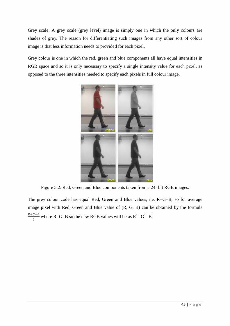
45 | P a g e

Grey scale: A grey scale (grey level) image is simply one in which the only colours are

shades of grey. The reason for differentiating such images from any other sort of colour

image is that less information needs to provided for each pixel.

Grey colour is one in which the red, green and blue components all have equal intensities in

RGB space and so it is only necessary to specify a single intensity value for each pixel, as

opposed to the three intensities needed to specify each pixels in full colour image.

Figure 5.2: Red, Green and Blue components taken from a 24- bit RGB images.

The grey colour code has equal Red, Green and Blue values, i.e. R=G=B, so for average

image pixel with Red, Green and Blue value of (R, G, B) can be obtained by the formula

where R=G=B so the new RGB values will be as R

’ =G

’ =B

’.

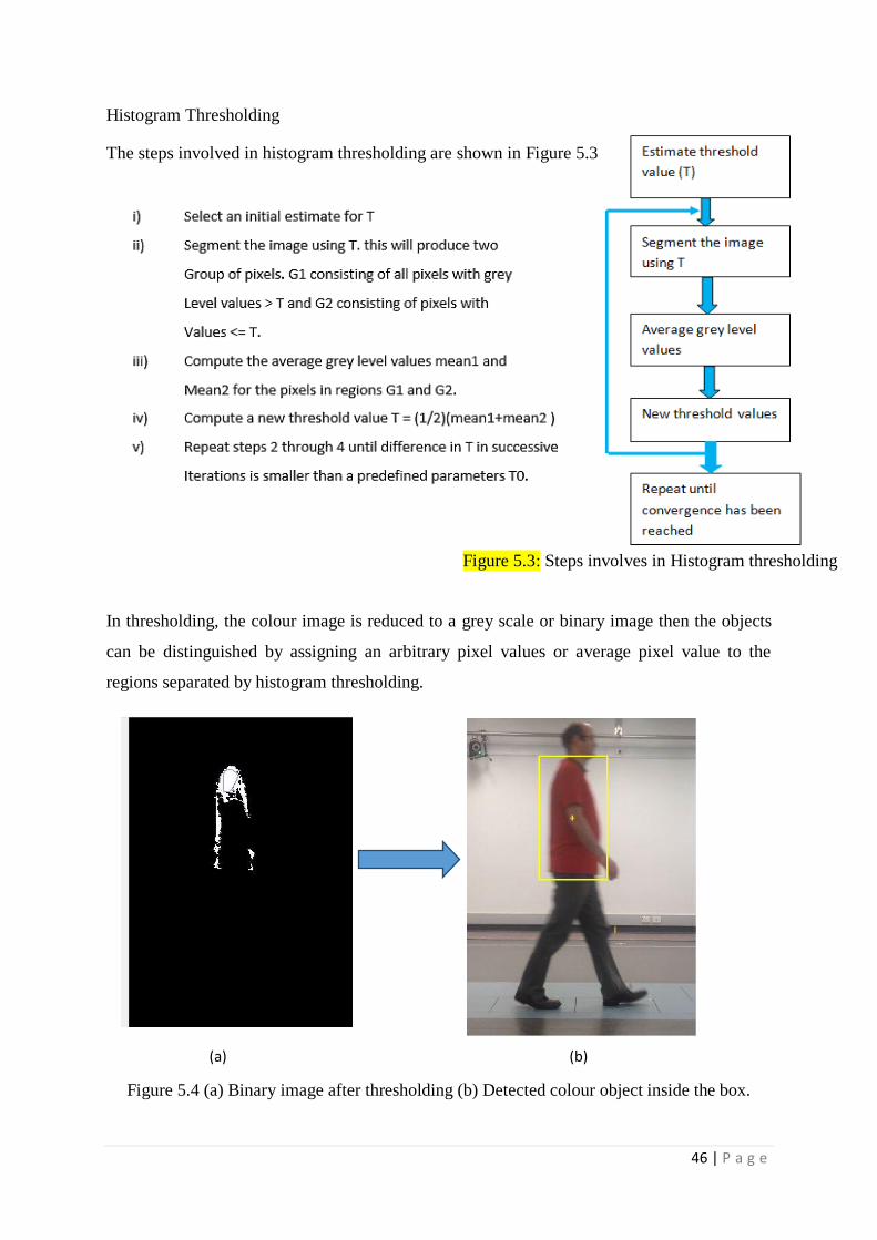
46 | P a g e

Histogram Thresholding

The steps involved in histogram thresholding are shown in Figure 5.3.

In thresholding, the colour image is reduced to a grey scale or binary image then the objects

can be distinguished by assigning an arbitrary pixel values or average pixel value to the

regions separated by histogram thresholding.

(a) (b)

Figure 5.4 (a) Binary image after thresholding (b) Detected colour object inside the box.

Figure 5.3: Steps involves in Histogram thresholding

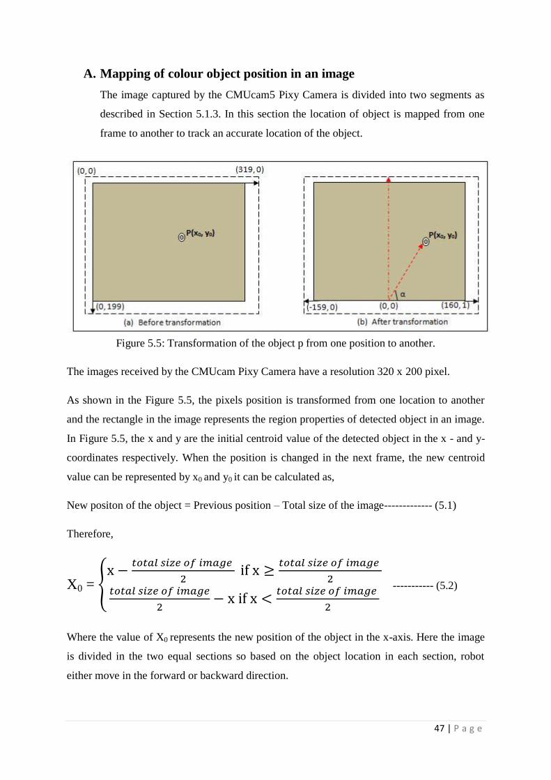
47 | P a g e

A. Mapping of colour object position in an image

The image captured by the CMUcam5 Pixy Camera is divided into two segments as

described in Section 5.1.3. In this section the location of object is mapped from one

frame to another to track an accurate location of the object.

Figure 5.5: Transformation of the object p from one position to another.

The images received by the CMUcam Pixy Camera have a resolution 320 x 200 pixel.

As shown in the Figure 5.5, the pixels position is transformed from one location to another

and the rectangle in the image represents the region properties of detected object in an image.

In Figure 5.5, the x and y are the initial centroid value of the detected object in the x - and y-

coordinates respectively. When the position is changed in the next frame, the new centroid

value can be represented by x0 and y0 it can be calculated as,

New positon of the object = Previous position – Total size of the image------------- (5.1)

Therefore,

X0 =

----------- (5.2)

Where the value of X0 represents the new position of the object in the x-axis. Here the image

is divided in the two equal sections so based on the object location in each section, robot

either move in the forward or backward direction.

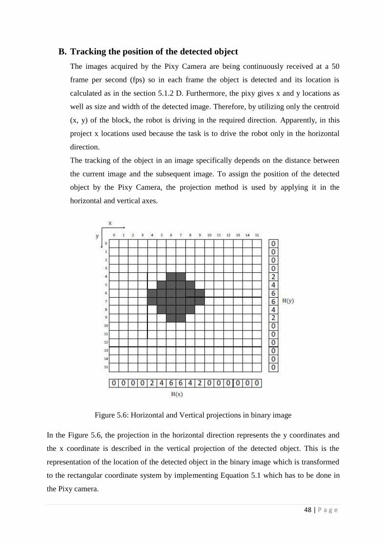
48 | P a g e

B. Tracking the position of the detected object

The images acquired by the Pixy Camera are being continuously received at a 50

frame per second (fps) so in each frame the object is detected and its location is

calculated as in the section 5.1.2 D. Furthermore, the pixy gives x and y locations as

well as size and width of the detected image. Therefore, by utilizing only the centroid

(x, y) of the block, the robot is driving in the required direction. Apparently, in this

project x locations used because the task is to drive the robot only in the horizontal

direction.

The tracking of the object in an image specifically depends on the distance between

the current image and the subsequent image. To assign the position of the detected

object by the Pixy Camera, the projection method is used by applying it in the

horizontal and vertical axes.

Figure 5.6: Horizontal and Vertical projections in binary image

In the Figure 5.6, the projection in the horizontal direction represents the y coordinates and

the x coordinate is described in the vertical projection of the detected object. This is the

representation of the location of the detected object in the binary image which is transformed

to the rectangular coordinate system by implementing Equation 5.1 which has to be done in

the Pixy camera.

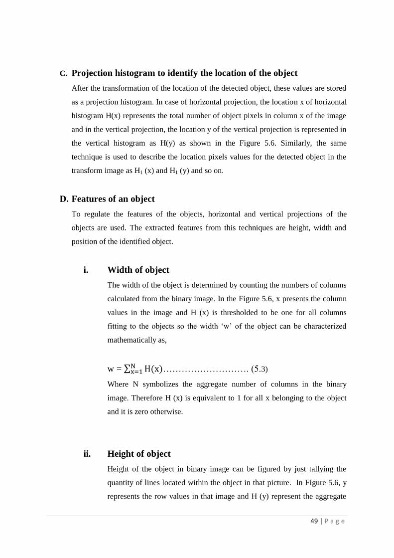
49 | P a g e

C. Projection histogram to identify the location of the object

After the transformation of the location of the detected object, these values are stored

as a projection histogram. In case of horizontal projection, the location x of horizontal

histogram H(x) represents the total number of object pixels in column x of the image

and in the vertical projection, the location y of the vertical projection is represented in

the vertical histogram as H(y) as shown in the Figure 5.6. Similarly, the same

technique is used to describe the location pixels values for the detected object in the

transform image as H1 (x) and H1 (y) and so on.

D. Features of an object

To regulate the features of the objects, horizontal and vertical projections of the

objects are used. The extracted features from this techniques are height, width and

position of the identified object.

i. Width of object

The width of the object is determined by counting the numbers of columns

calculated from the binary image. In the Figure 5.6, x presents the column

values in the image and H (x) is thresholded to be one for all columns

fitting to the objects so the width ‘w’ of the object can be characterized

mathematically as,

w = ………………………. (5.3)

Where N symbolizes the aggregate number of columns in the binary

image. Therefore H (x) is equivalent to 1 for all x belonging to the object

and it is zero otherwise.

ii. Height of object

Height of the object in binary image can be figured by just tallying the

quantity of lines located within the object in that picture. In Figure 5.6, y

represents the row values in that image and H (y) represent the aggregate

50 | P a g e

number of the pixels in the line y. Presently, if H (y) is a threshold to be 1

for all the columns belonging to the object location, then the height h of an

object be spoken numerically as,

h = ………………………. (5.4)

In Equation (5.4), M denotes the total number of rows in the binary image

and H (y) is equal to 1 for all rows that belongs to the object and it is 0

otherwise.

iii. X –Position of object

To determine the accurate location of the image in the binary image, it is

essential to estimate the central point of the object on x axis and y axis.

The x position of the object can be determined by using the following

formula,

X =

………………………. (5.5)

In Equation (5.5), w is obtained from the equation (5.3) where N indicates

the total number of the columns.

iv. Y- Position of object

The Central location of detecting object on Y-axis can be considered by

using Equation (5.6)

Y =

………………………. (5.6)

In the above Equation (5.6), h can be calculated from the Equation (5.4)

and the value of M is represented as the total number of the rows in the

binary image.

51 | P a g e

5.1.3 Experimental analysis of object detection and tracking

A. Introduction

The automated camera system is tracking an object from one location to another. That means

to achieve the succeeding position it has to travel some distance in a certain time. Therefore,

the distance travelled by the system in a certain period of time gives the average speed of that

system. Hence the purpose of this section is to analyse the average speed of the object as well

as the respective average speed of the automated camera tracking system to ensure whether it

is able to meet the desired average speed of human walking or not.

For this purpose two different methods has been implemented where the first method is called

frame analysis (FA) and the second method is called image processing (IA) method. An

average speed of the object from FA and average speed from IA compare with each other to

analyse the accuracy of the two different object detection methods.

i. Frame Analysis (FA) Method

In the FA Method, the average speed of the object in a recorded video captured by the video

camera attached to the robot is calculated manually by measuring the distance travelled by

the object and total number of frames to travel the same distance. The distance is measured

by taking the standard force plate pit measurement as the reference distance as shown in the

Figure 5.7. So if the person started walking from the one end as shown in the Figure 5.8. The

distance travelled by the person to reach the other end is considered as 3.06m. The reference

distance can be any of the distance measurements shown in the Figure. 5.7. Moreover, the

duration to travel that distance can be measured with the number of frame counts from one

end to another or if the frame rate of the camera is known then it can be calculated as, time

(sec) =

. As soon as the distance and time is known, the average speed of that object

can be determined. This average speed calculated from the distance and video frame is used

as a reference speed to compare the detection accuracy of the object detection and tracking

method.

52 | P a g e

ii. Image Analysis (IA) Method

Likewise, when the object moves from one frame to another, the distance travelled by that

object is calculated as the change in distance from one frame to another. Also that distance is

stored as an array in matrix form. The process continues throughout the experiment.

Therefore, in the IA Method, the actual speed is calculated from object detection method

using digital image processing rather to doing it manually.

Likewise, the average speed of the robot is manually calculated by measuring the total

distance traveled by robot and total time taken to travel that distance.

Furthermore, the average speed calculated manually from FA Method and the average speed

calculated from IA are evaluated to analyse the location accuracy of the robot with the color

detection and tracking method.

Finally the overall system performance can be compared with the average walking speed of

the person which is normally 1.5 m/s.

B. Experimental Analysis

As discussed in the previous section, the performance can be analyses by comparing the

average speed. So here the average speed of the object from FA Method and instantaneous

speed of object from IA Method are compared with each other. Both FA & IA Methods are

conducted with the same recorded video.

i. Calculation of average speed from Frame Analysis (FA) Method

The average speed of any object in a recorded video can be determined by measuring the total

distance travelled from one point to another divided by the total number of frames or total

time taken from one point to another.

Therefore,

Average Speed (SF) =

= cm/frame or cm/sec

(5.7)

The unit is cm/n or cm/sec. Where n= frame.

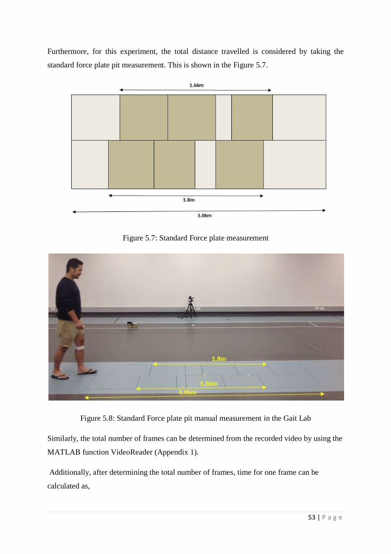
53 | P a g e

Furthermore, for this experiment, the total distance travelled is considered by taking the

standard force plate pit measurement. This is shown in the Figure 5.7.

Figure 5.7: Standard Force plate measurement

Figure 5.8: Standard Force plate pit manual measurement in the Gait Lab

Similarly, the total number of frames can be determined from the recorded video by using the

MATLAB function VideoReader (Appendix 1).

Additionally, after determining the total number of frames, time for one frame can be

calculated as,

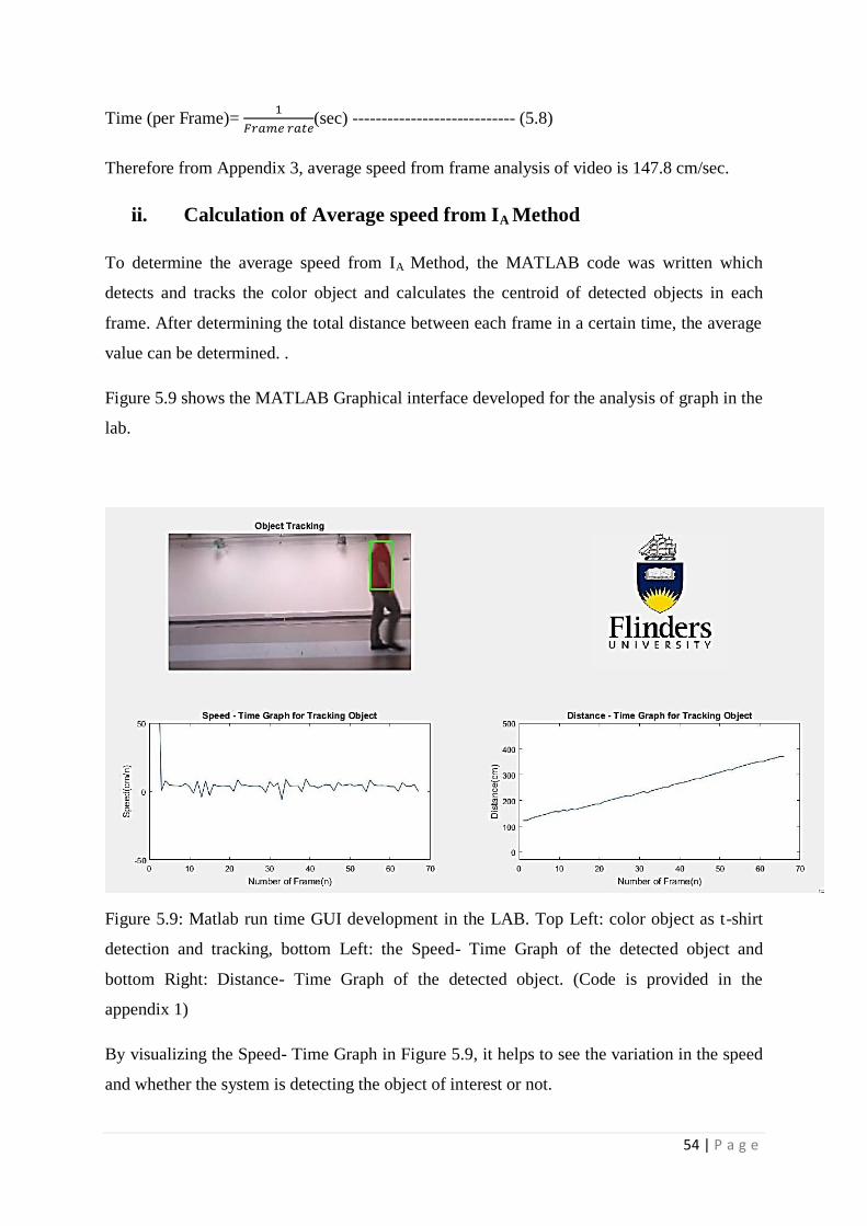
54 | P a g e

Time (per Frame)=

(sec) ---------------------------- (5.8)

Therefore from Appendix 3, average speed from frame analysis of video is 147.8 cm/sec.

ii. Calculation of Average speed from IA Method

To determine the average speed from IA Method, the MATLAB code was written which

detects and tracks the color object and calculates the centroid of detected objects in each

frame. After determining the total distance between each frame in a certain time, the average

value can be determined. .

Figure 5.9 shows the MATLAB Graphical interface developed for the analysis of graph in the

lab.

Figure 5.9: Matlab run time GUI development in the LAB. Top Left: color object as t-shirt

detection and tracking, bottom Left: the Speed- Time Graph of the detected object and

bottom Right: Distance- Time Graph of the detected object. (Code is provided in the

appendix 1)

By visualizing the Speed- Time Graph in Figure 5.9, it helps to see the variation in the speed

and whether the system is detecting the object of interest or not.

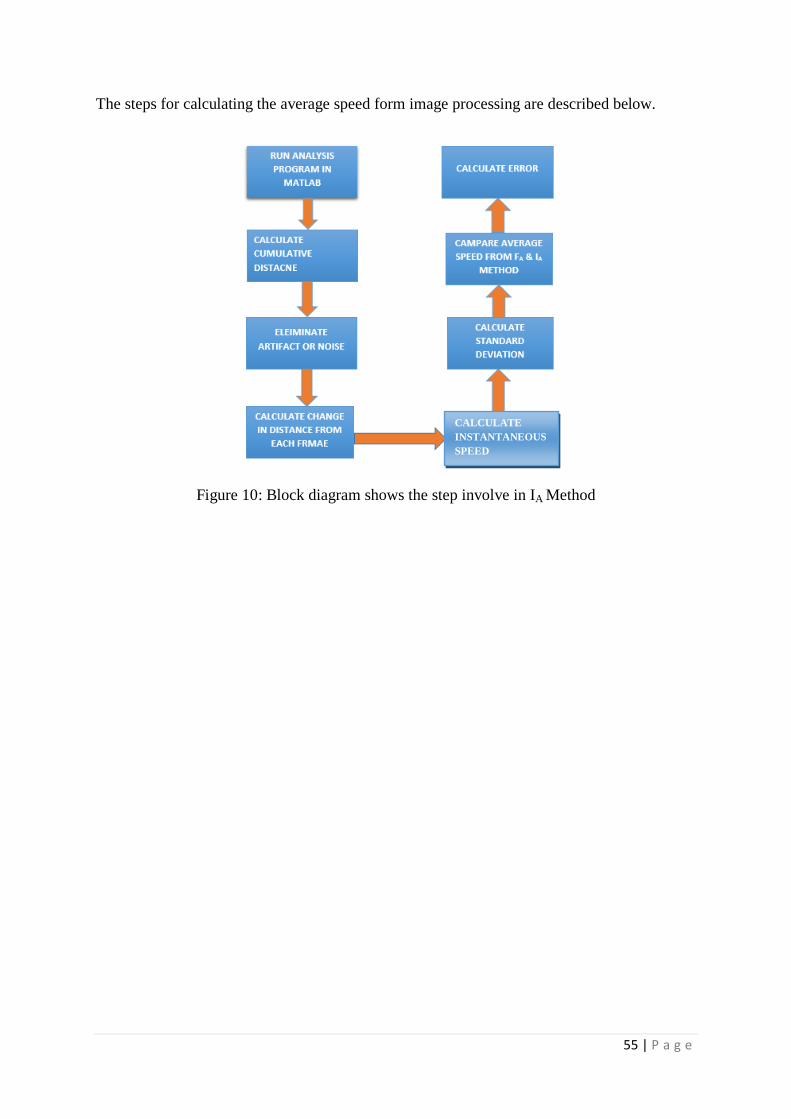
55 | P a g e

The steps for calculating the average speed form image processing are described below.

Figure 10: Block diagram shows the step involve in IA Method

CALCULATE

INSTANTANEOUS

SPEED

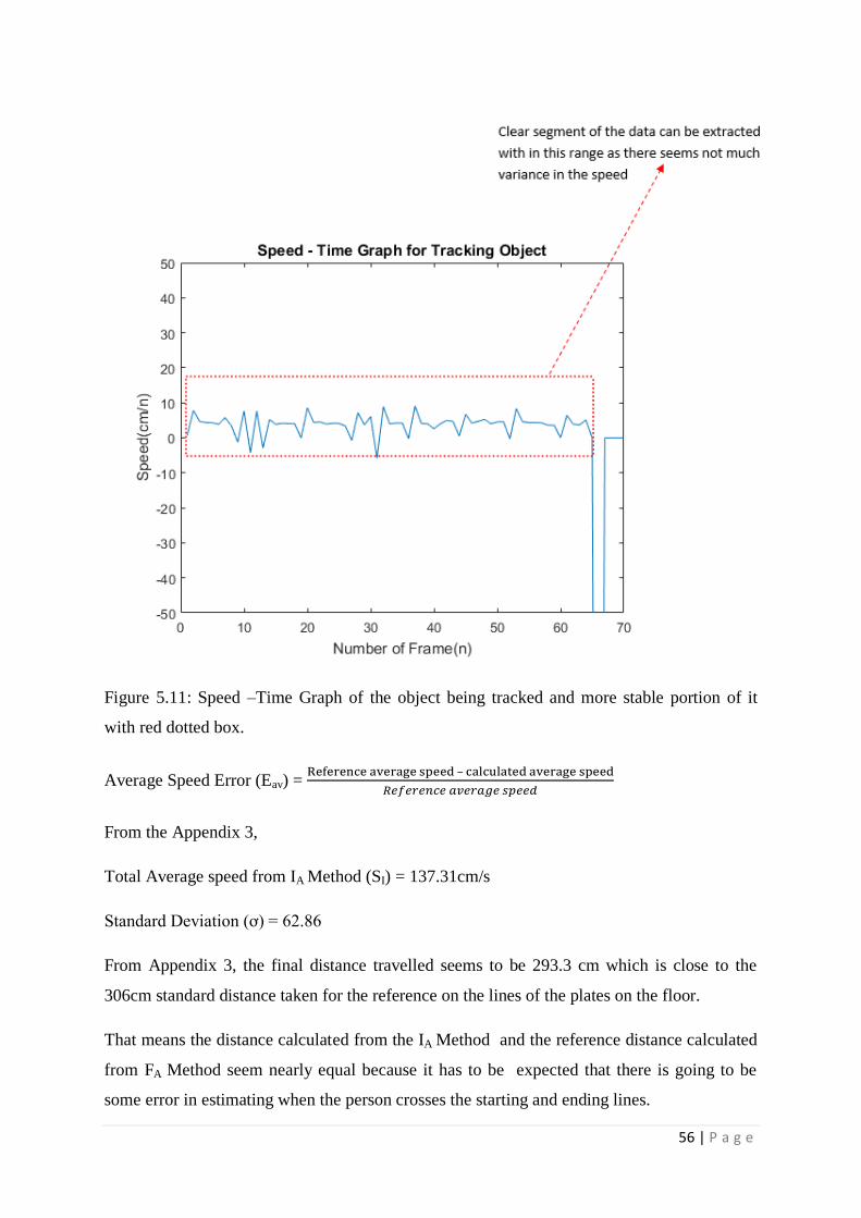
56 | P a g e

Figure 5.11: Speed –Time Graph of the object being tracked and more stable portion of it

with red dotted box.

Average Speed Error (Eav) = –

From the Appendix 3,

Total Average speed from IA Method (SI) = 137.31cm/s

Standard Deviation (ơ) = 62.86

From Appendix 3, the final distance travelled seems to be 293.3 cm which is close to the

306cm standard distance taken for the reference on the lines of the plates on the floor.

That means the distance calculated from the IA Method and the reference distance calculated

from FA Method seem nearly equal because it has to be expected that there is going to be

some error in estimating when the person crosses the starting and ending lines.

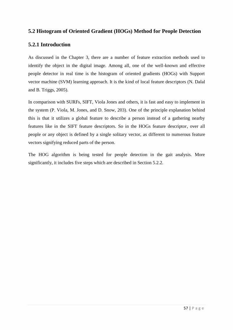
57 | P a g e

5.2 Histogram of Oriented Gradient (HOGs) Method for People Detection

5.2.1 Introduction

As discussed in the Chapter 3, there are a number of feature extraction methods used to

identify the object in the digital image. Among all, one of the well-known and effective

people detector in real time is the histogram of oriented gradients (HOGs) with Support

vector machine (SVM) learning approach. It is the kind of local feature descriptors (N. Dalal

and B. Triggs, 2005).

In comparison with SURFs, SIFT, Viola Jones and others, it is fast and easy to implement in

the system (P. Viola, M. Jones, and D. Snow, 203). One of the principle explanation behind

this is that it utilizes a global feature to describe a person instead of a gathering nearby

features like in the SIFT feature descriptors. So in the HOGs feature descriptor, over all

people or any object is defined by a single solitary vector, as different to numerous feature

vectors signifying reduced parts of the person.

The HOG algorithm is being tested for people detection in the gait analysis. More

significantly, it includes five steps which are described in Section 5.2.2.

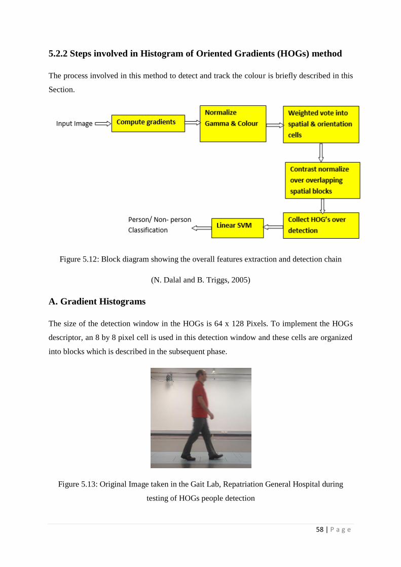
58 | P a g e

5.2.2 Steps involved in Histogram of Oriented Gradients (HOGs) method

The process involved in this method to detect and track the colour is briefly described in this

Section.

Figure 5.12: Block diagram showing the overall features extraction and detection chain

(N. Dalal and B. Triggs, 2005)

A. Gradient Histograms

The size of the detection window in the HOGs is 64 x 128 Pixels. To implement the HOGs

descriptor, an 8 by 8 pixel cell is used in this detection window and these cells are organized

into blocks which is described in the subsequent phase.

Figure 5.13: Original Image taken in the Gait Lab, Repatriation General Hospital during

testing of HOGs people detection

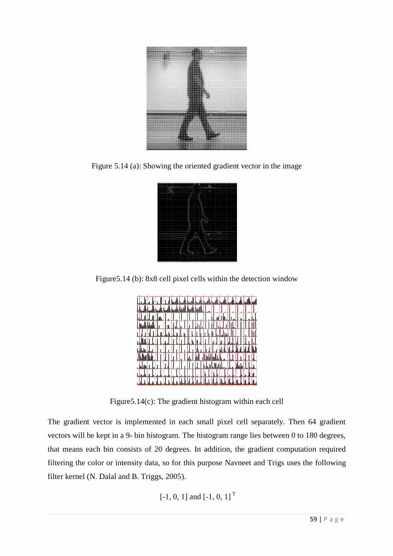
59 | P a g e

Figure 5.14 (a): Showing the oriented gradient vector in the image

Figure5.14 (b): 8x8 cell pixel cells within the detection window

Figure5.14(c): The gradient histogram within each cell

The gradient vector is implemented in each small pixel cell separately. Then 64 gradient

vectors will be kept in a 9- bin histogram. The histogram range lies between 0 to 180 degrees,

that means each bin consists of 20 degrees. In addition, the gradient computation required

filtering the color or intensity data, so for this purpose Navneet and Trigs uses the following

filter kernel (N. Dalal and B. Triggs, 2005).

[-1, 0, 1] and [-1, 0, 1] T

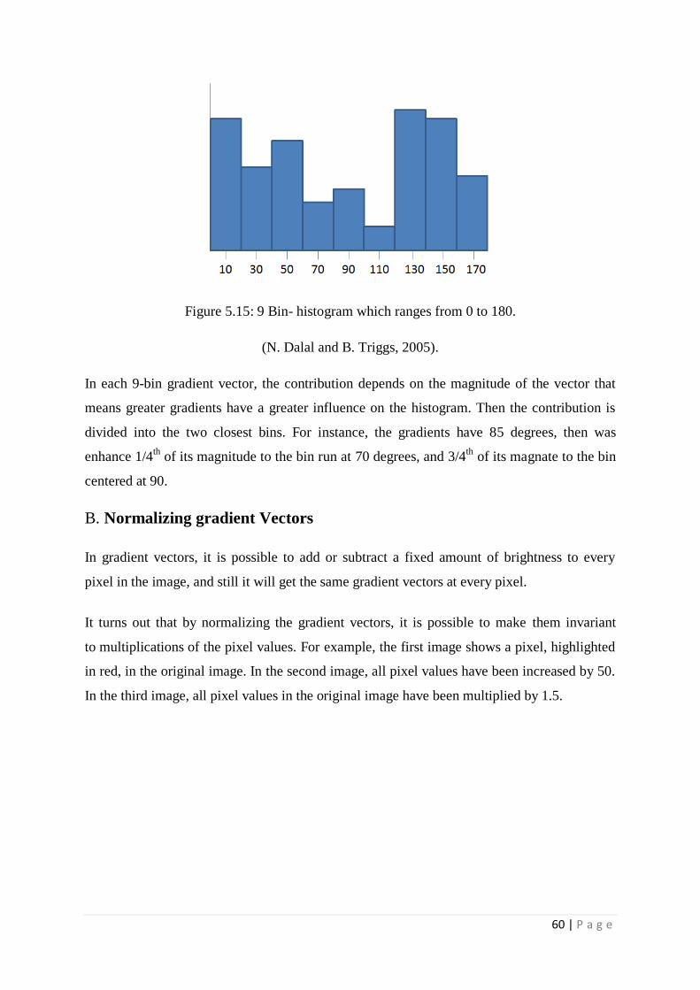
60 | P a g e

Figure 5.15: 9 Bin- histogram which ranges from 0 to 180.

(N. Dalal and B. Triggs, 2005).

In each 9-bin gradient vector, the contribution depends on the magnitude of the vector that

means greater gradients have a greater influence on the histogram. Then the contribution is

divided into the two closest bins. For instance, the gradients have 85 degrees, then was

enhance 1/4th

of its magnitude to the bin run at 70 degrees, and 3/4th

of its magnate to the bin

centered at 90.

B. Normalizing gradient Vectors

In gradient vectors, it is possible to add or subtract a fixed amount of brightness to every

pixel in the image, and still it will get the same gradient vectors at every pixel.

It turns out that by normalizing the gradient vectors, it is possible to make them invariant

to multiplications of the pixel values. For example, the first image shows a pixel, highlighted

in red, in the original image. In the second image, all pixel values have been increased by 50.

In the third image, all pixel values in the original image have been multiplied by 1.5.

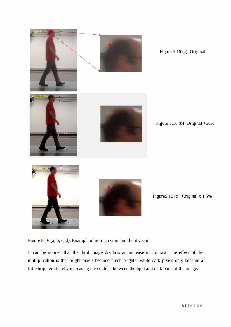
61 | P a g e

Figure 5.16 (a, b, c, d): Example of normalization gradient vector

It can be noticed that the third image displays an increase in contrast. The effect of the

multiplication is that bright pixels became much brighter while dark pixels only became a

little brighter, thereby increasing the contrast between the light and dark parts of the image.

Figure 5.16 (a): Original

Figure 5.16 (b): Original +50%

Figure5.16 (c): Original x 1.5%

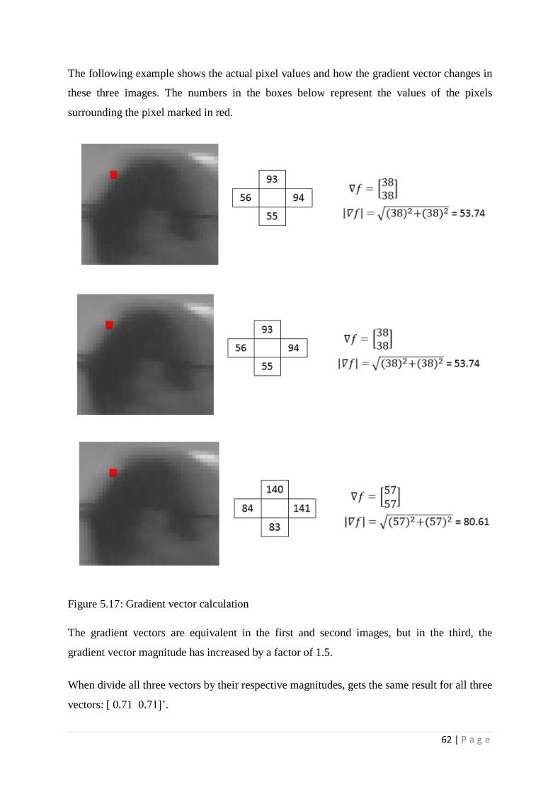
62 | P a g e

The following example shows the actual pixel values and how the gradient vector changes in

these three images. The numbers in the boxes below represent the values of the pixels

surrounding the pixel marked in red.

Figure 5.17: Gradient vector calculation

The gradient vectors are equivalent in the first and second images, but in the third, the

gradient vector magnitude has increased by a factor of 1.5.

When divide all three vectors by their respective magnitudes, gets the same result for all three

vectors: [ 0.71 0.71]’.

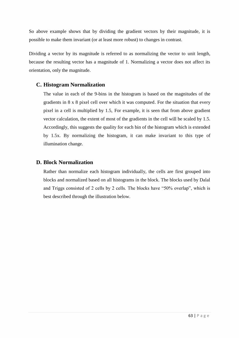
63 | P a g e

So above example shows that by dividing the gradient vectors by their magnitude, it is

possible to make them invariant (or at least more robust) to changes in contrast.

Dividing a vector by its magnitude is referred to as normalizing the vector to unit length,

because the resulting vector has a magnitude of 1. Normalizing a vector does not affect its

orientation, only the magnitude.

C. Histogram Normalization

The value in each of the 9-bins in the histogram is based on the magnitudes of the

gradients in 8 x 8 pixel cell over which it was computed. For the situation that every

pixel in a cell is multiplied by 1.5, For example, it is seen that from above gradient

vector calculation, the extent of most of the gradients in the cell will be scaled by 1.5.

Accordingly, this suggests the quality for each bin of the histogram which is extended

by 1.5x. By normalizing the histogram, it can make invariant to this type of

illumination change.

D. Block Normalization

Rather than normalize each histogram individually, the cells are first grouped into

blocks and normalized based on all histograms in the block. The blocks used by Dalal

and Triggs consisted of 2 cells by 2 cells. The blocks have “50% overlap”, which is

best described through the illustration below.

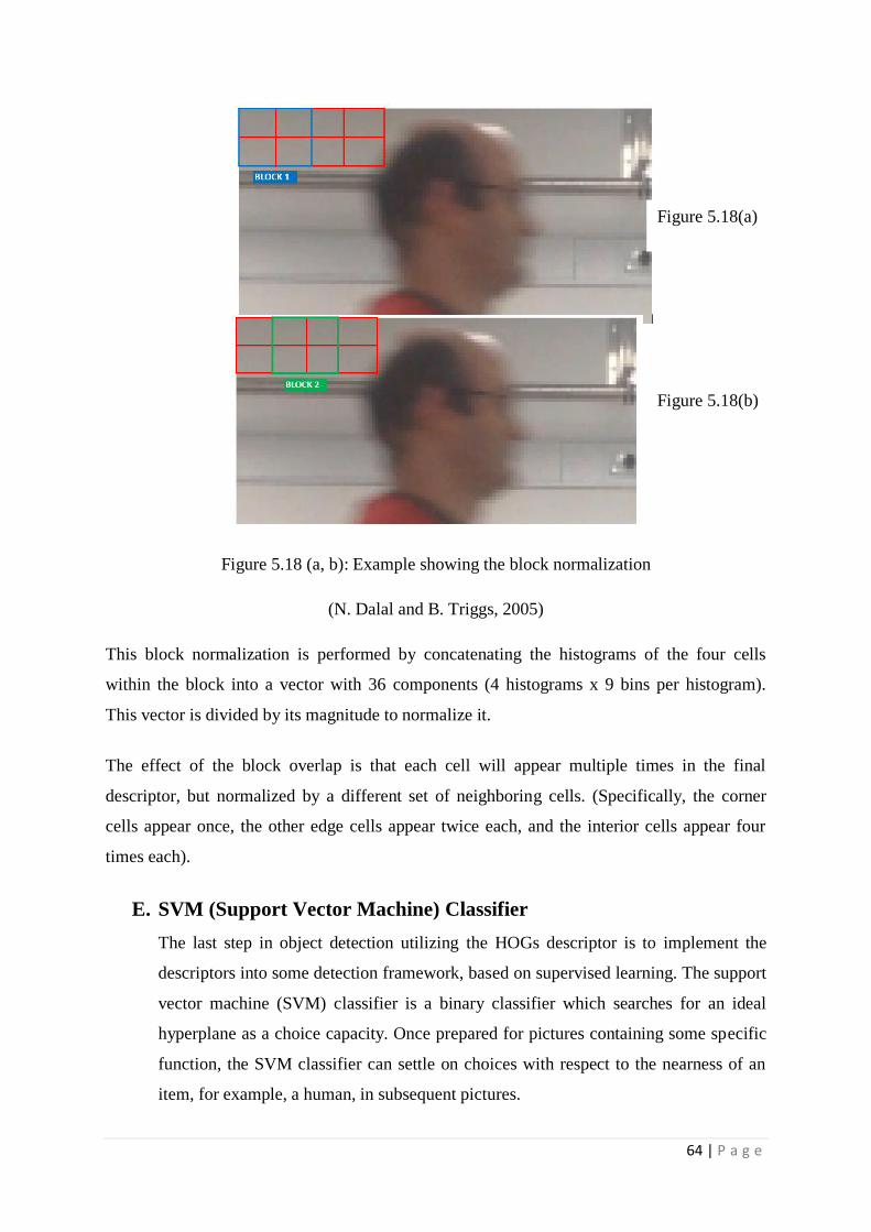
64 | P a g e

Figure 5.18 (a, b): Example showing the block normalization

(N. Dalal and B. Triggs, 2005)

This block normalization is performed by concatenating the histograms of the four cells

within the block into a vector with 36 components (4 histograms x 9 bins per histogram).

This vector is divided by its magnitude to normalize it.

The effect of the block overlap is that each cell will appear multiple times in the final

descriptor, but normalized by a different set of neighboring cells. (Specifically, the corner

cells appear once, the other edge cells appear twice each, and the interior cells appear four

times each).

E. SVM (Support Vector Machine) Classifier

The last step in object detection utilizing the HOGs descriptor is to implement the

descriptors into some detection framework, based on supervised learning. The support

vector machine (SVM) classifier is a binary classifier which searches for an ideal

hyperplane as a choice capacity. Once prepared for pictures containing some specific

function, the SVM classifier can settle on choices with respect to the nearness of an

item, for example, a human, in subsequent pictures.

Figure 5.18(a)

Figure 5.18(b)

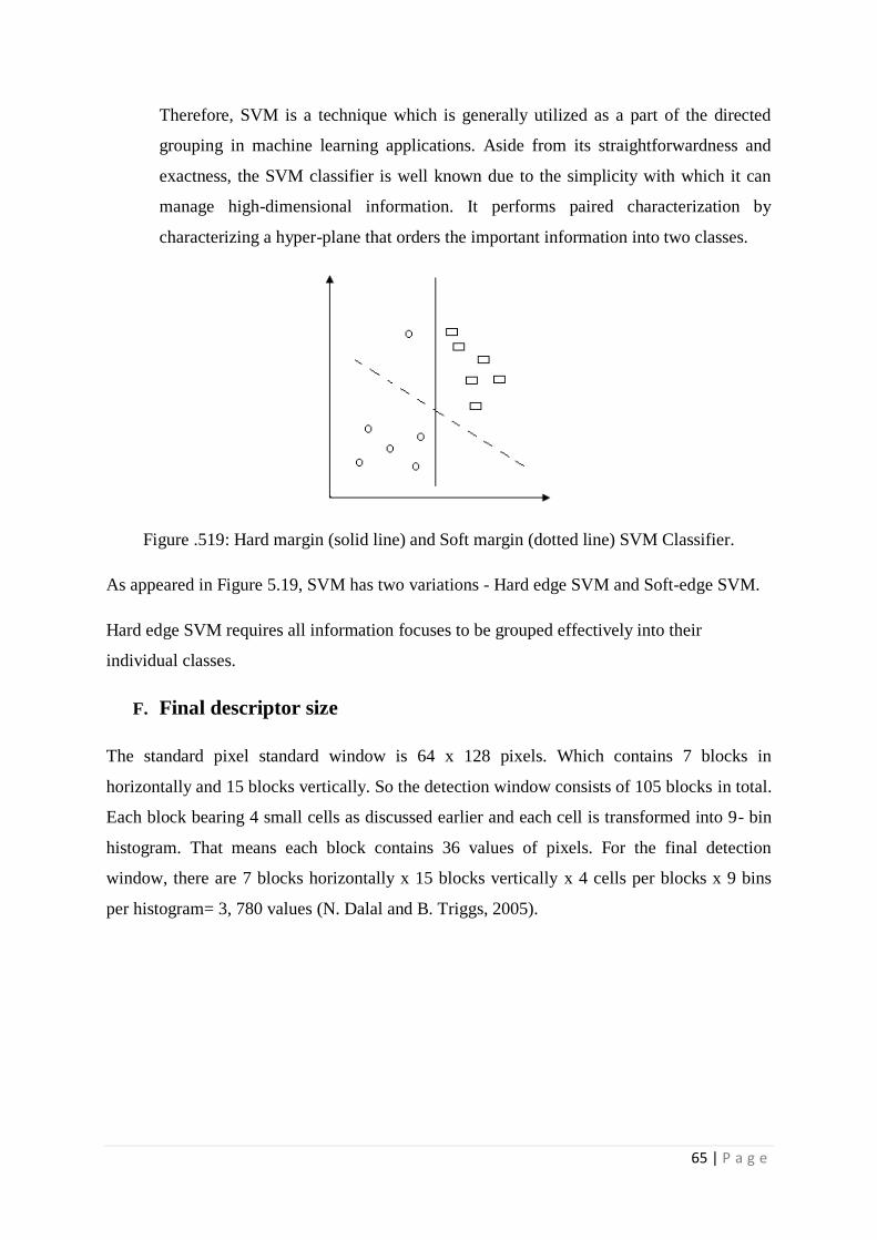
65 | P a g e

Therefore, SVM is a technique which is generally utilized as a part of the directed

grouping in machine learning applications. Aside from its straightforwardness and

exactness, the SVM classifier is well known due to the simplicity with which it can

manage high-dimensional information. It performs paired characterization by

characterizing a hyper-plane that orders the important information into two classes.

Figure .519: Hard margin (solid line) and Soft margin (dotted line) SVM Classifier.

As appeared in Figure 5.19, SVM has two variations - Hard edge SVM and Soft-edge SVM.

Hard edge SVM requires all information focuses to be grouped effectively into their

individual classes.

F. Final descriptor size

The standard pixel standard window is 64 x 128 pixels. Which contains 7 blocks in

horizontally and 15 blocks vertically. So the detection window consists of 105 blocks in total.

Each block bearing 4 small cells as discussed earlier and each cell is transformed into 9- bin

histogram. That means each block contains 36 values of pixels. For the final detection

window, there are 7 blocks horizontally x 15 blocks vertically x 4 cells per blocks x 9 bins

per histogram= 3, 780 values (N. Dalal and B. Triggs, 2005).

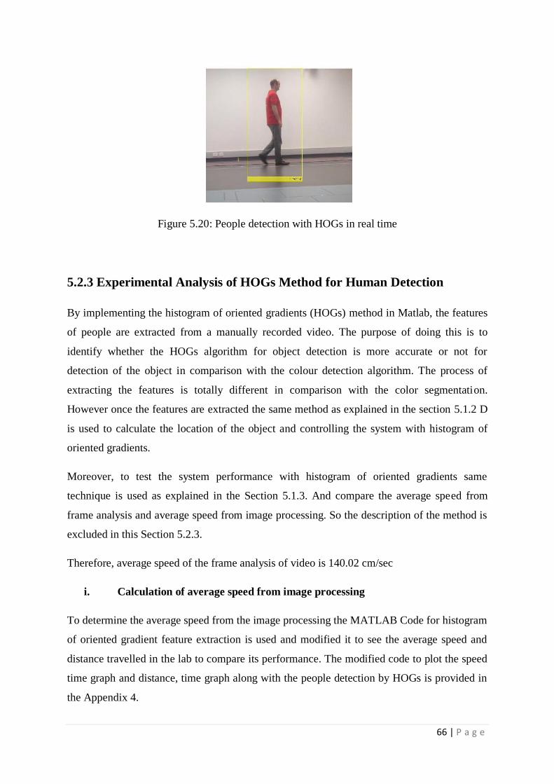
66 | P a g e

Figure 5.20: People detection with HOGs in real time

5.2.3 Experimental Analysis of HOGs Method for Human Detection

By implementing the histogram of oriented gradients (HOGs) method in Matlab, the features

of people are extracted from a manually recorded video. The purpose of doing this is to

identify whether the HOGs algorithm for object detection is more accurate or not for

detection of the object in comparison with the colour detection algorithm. The process of

extracting the features is totally different in comparison with the color segmentation.

However once the features are extracted the same method as explained in the section 5.1.2 D

is used to calculate the location of the object and controlling the system with histogram of

oriented gradients.

Moreover, to test the system performance with histogram of oriented gradients same

technique is used as explained in the Section 5.1.3. And compare the average speed from

frame analysis and average speed from image processing. So the description of the method is

excluded in this Section 5.2.3.

Therefore, average speed of the frame analysis of video is 140.02 cm/sec

i. Calculation of average speed from image processing

To determine the average speed from the image processing the MATLAB Code for histogram

of oriented gradient feature extraction is used and modified it to see the average speed and

distance travelled in the lab to compare its performance. The modified code to plot the speed

time graph and distance, time graph along with the people detection by HOGs is provided in

the Appendix 4.

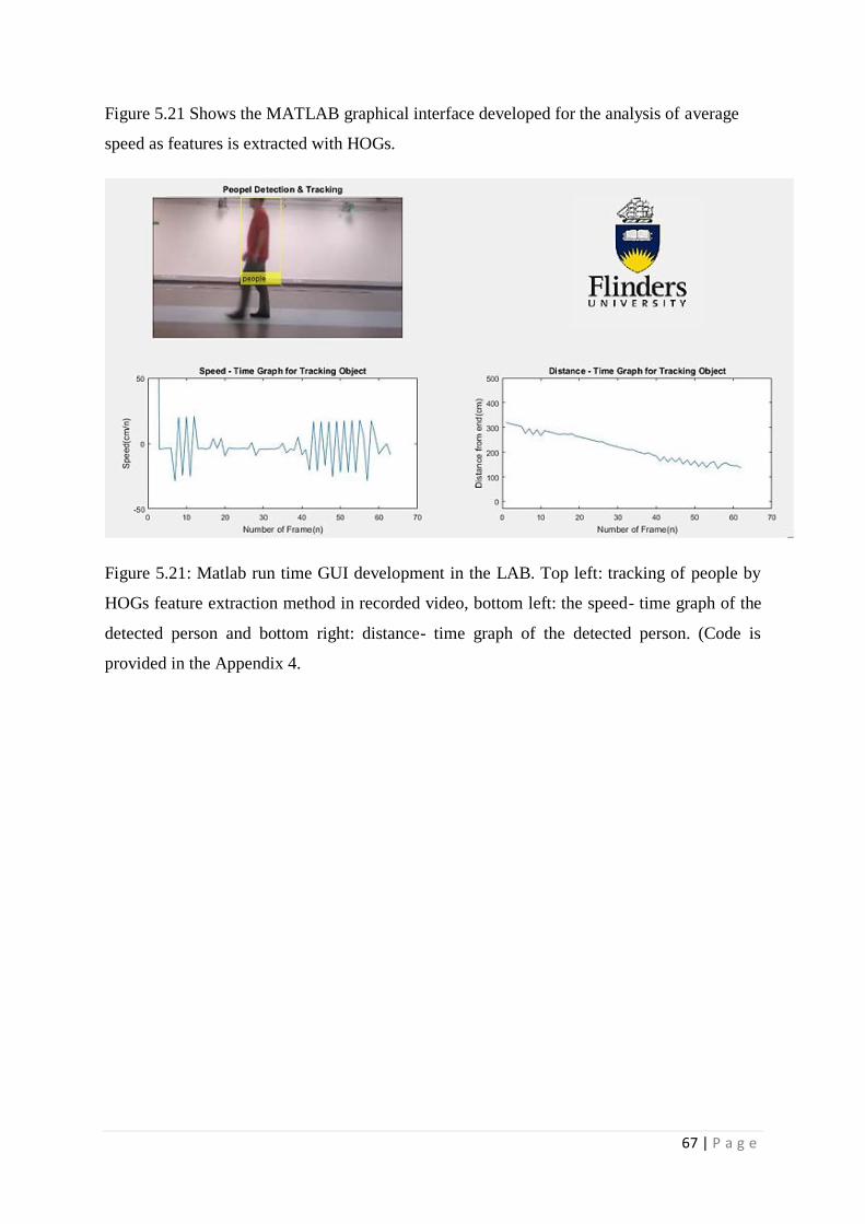
67 | P a g e

Figure 5.21 Shows the MATLAB graphical interface developed for the analysis of average

speed as features is extracted with HOGs.

Figure 5.21: Matlab run time GUI development in the LAB. Top left: tracking of people by

HOGs feature extraction method in recorded video, bottom left: the speed- time graph of the

detected person and bottom right: distance- time graph of the detected person. (Code is

provided in the Appendix 4.

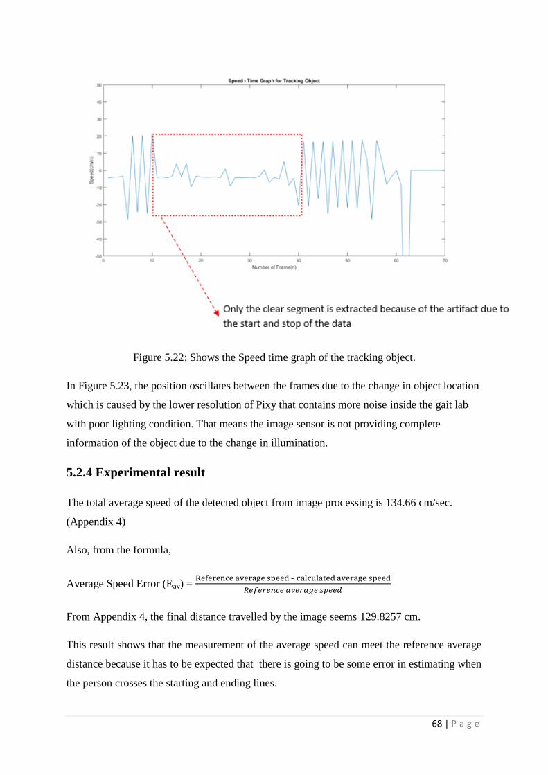
68 | P a g e

Figure 5.22: Shows the Speed time graph of the tracking object.

In Figure 5.23, the position oscillates between the frames due to the change in object location

which is caused by the lower resolution of Pixy that contains more noise inside the gait lab

with poor lighting condition. That means the image sensor is not providing complete

information of the object due to the change in illumination.

5.2.4 Experimental result

The total average speed of the detected object from image processing is 134.66 cm/sec.

(Appendix 4)

Also, from the formula,

Average Speed Error (Eav) = –

From Appendix 4, the final distance travelled by the image seems 129.8257 cm.

This result shows that the measurement of the average speed can meet the reference average

distance because it has to be expected that there is going to be some error in estimating when

the person crosses the starting and ending lines.

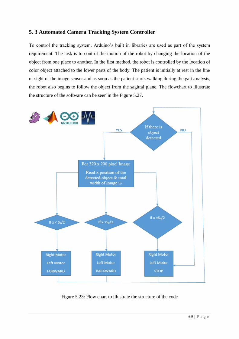
69 | P a g e

5. 3 Automated Camera Tracking System Controller

To control the tracking system, Arduino’s built in libraries are used as part of the system

requirement. The task is to control the motion of the robot by changing the location of the

object from one place to another. In the first method, the robot is controlled by the location of

color object attached to the lower parts of the body. The patient is initially at rest in the line

of sight of the image sensor and as soon as the patient starts walking during the gait analysis,

the robot also begins to follow the object from the sagittal plane. The flowchart to illustrate

the structure of the software can be seen in the Figure 5.27.

Figure 5.23: Flow chart to illustrate the structure of the code

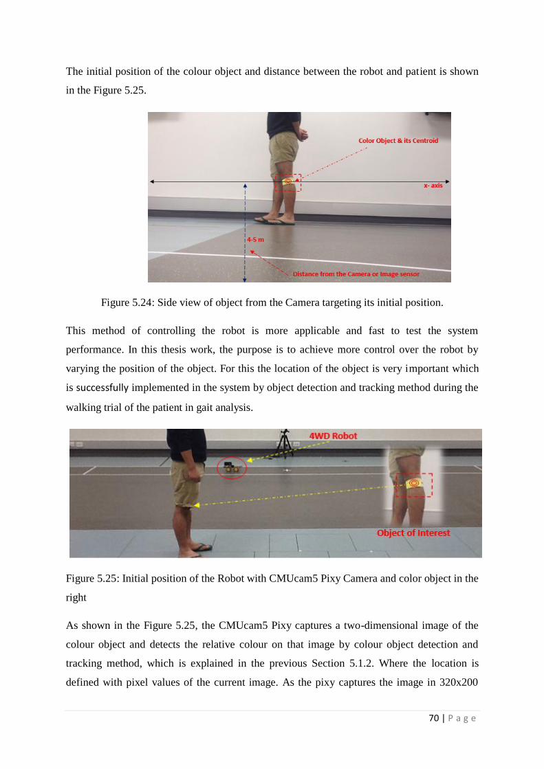
70 | P a g e

The initial position of the colour object and distance between the robot and patient is shown

in the Figure 5.25.

Figure 5.24: Side view of object from the Camera targeting its initial position.

This method of controlling the robot is more applicable and fast to test the system

performance. In this thesis work, the purpose is to achieve more control over the robot by

varying the position of the object. For this the location of the object is very important which

is successfully implemented in the system by object detection and tracking method during the

walking trial of the patient in gait analysis.

Figure 5.25: Initial position of the Robot with CMUcam5 Pixy Camera and color object in the

right

As shown in the Figure 5.25, the CMUcam5 Pixy captures a two-dimensional image of the

colour object and detects the relative colour on that image by colour object detection and

tracking method, which is explained in the previous Section 5.1.2. Where the location is

defined with pixel values of the current image. As the pixy captures the image in 320x200

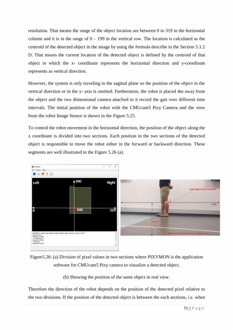
71 | P a g e

resolution. That means the range of the object location are between 0 to 319 in the horizontal

column and it is in the range of 0 – 199 in the vertical row. The location is calculated as the

centroid of the detected object in the image by using the formula describe in the Section 5.1.2

D. That means the current location of the detected object is defined by the centroid of that

object in which the x- coordinate represents the horizontal direction and y-coordinate

represents as vertical direction.

However, the system is only traveling in the sagittal plane so the position of the object in the

vertical direction or in the y- axis is omitted. Furthermore, the robot is placed 4m away from

the object and the two dimensional camera attached to it record the gait over different time

intervals. The initial position of the robot with the CMUcam5 Pixy Camera and the view

from the robot Image Sensor is shown in the Figure 5.25.

To control the robot movement in the horizontal direction, the position of the object along the

x coordinate is divided into two sections. Each position in the two sections of the detected

object is responsible to move the robot either in the forward or backward direction. These

segments are well illustrated in the Figure 5.26 (a).

Figure5.26: (a) Division of pixel values in two sections where PIXYMON is the application

software for CMUcam5 Pixy camera to visualize a detected object.

(b) Showing the position of the same object in real view.

Therefore the direction of the robot depends on the position of the detected pixel relative to

the two divisions. If the position of the detected object is between the each sections, i.e. when

0 319

Left

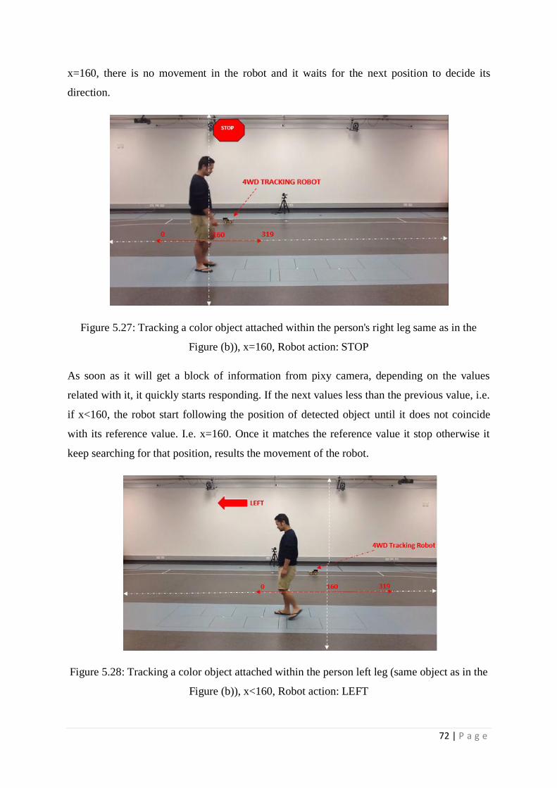
72 | P a g e

x=160, there is no movement in the robot and it waits for the next position to decide its

direction.

Figure 5.27: Tracking a color object attached within the person's right leg same as in the

Figure (b)), x=160, Robot action: STOP

As soon as it will get a block of information from pixy camera, depending on the values

related with it, it quickly starts responding. If the next values less than the previous value, i.e.

if x<160, the robot start following the position of detected object until it does not coincide

with its reference value. I.e. x=160. Once it matches the reference value it stop otherwise it

keep searching for that position, results the movement of the robot.

Figure 5.28: Tracking a color object attached within the person left leg (same object as in the

Figure (b)), x<160, Robot action: LEFT

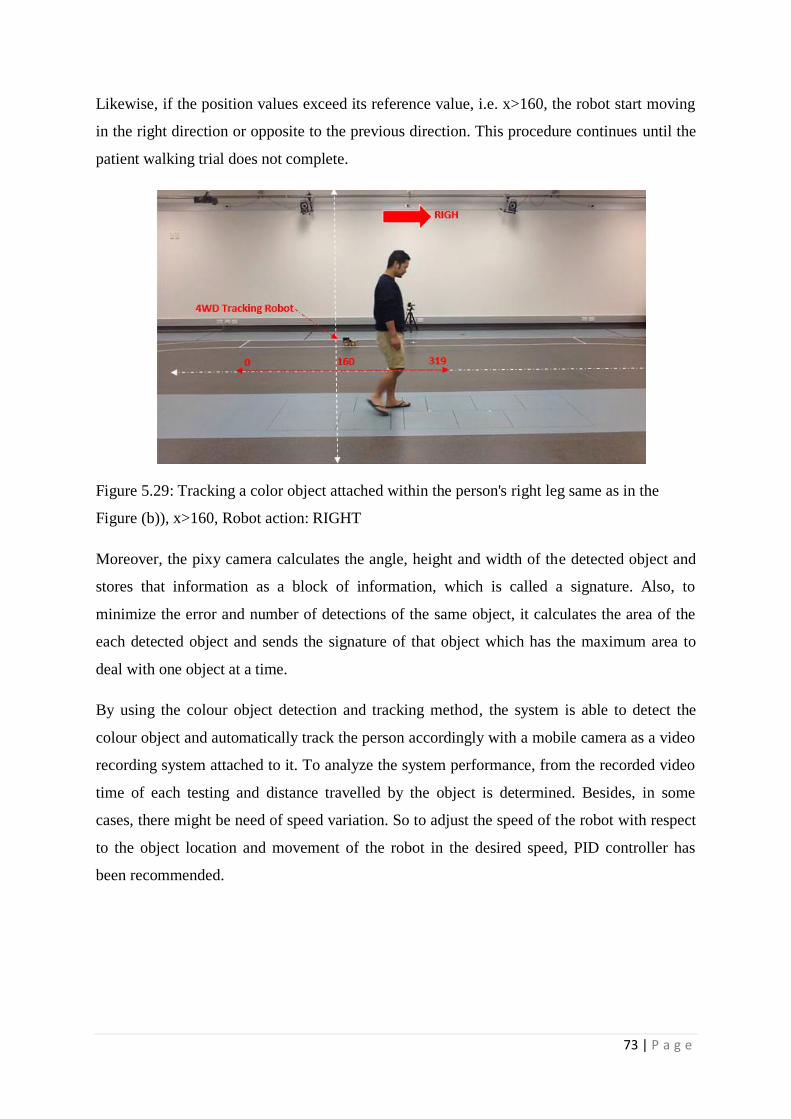
73 | P a g e

Likewise, if the position values exceed its reference value, i.e. x>160, the robot start moving

in the right direction or opposite to the previous direction. This procedure continues until the

patient walking trial does not complete.

Figure 5.29: Tracking a color object attached within the person's right leg same as in the

Figure (b)), x>160, Robot action: RIGHT

Moreover, the pixy camera calculates the angle, height and width of the detected object and

stores that information as a block of information, which is called a signature. Also, to

minimize the error and number of detections of the same object, it calculates the area of the

each detected object and sends the signature of that object which has the maximum area to

deal with one object at a time.

By using the colour object detection and tracking method, the system is able to detect the

colour object and automatically track the person accordingly with a mobile camera as a video

recording system attached to it. To analyze the system performance, from the recorded video

time of each testing and distance travelled by the object is determined. Besides, in some

cases, there might be need of speed variation. So to adjust the speed of the robot with respect

to the object location and movement of the robot in the desired speed, PID controller has

been recommended.

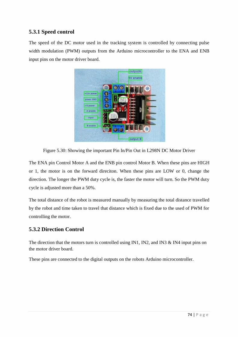
74 | P a g e

5.3.1 Speed control

The speed of the DC motor used in the tracking system is controlled by connecting pulse

width modulation (PWM) outputs from the Arduino microcontroller to the ENA and ENB

input pins on the motor driver board.

Figure 5.30: Showing the important Pin In/Pin Out in L298N DC Motor Driver

The ENA pin Control Motor A and the ENB pin control Motor B. When these pins are HIGH

or 1, the motor is on the forward direciton. When these pins are LOW or 0, change the

direction. The longer the PWM duty cycle is, the faster the motor will turn. So the PWM duty

cycle is adjusted more than a 50%.

The total distance of the robot is measured manually by measuring the total distance travelled

by the robot and time taken to travel that distance which is fixed due to the used of PWM for

controlling the motor.

5.3.2 Direction Control

The direction that the motors turn is controlled using IN1, IN2, and IN3 & IN4 input pins on

the motor driver board.

These pins are connected to the digital outputs on the robots Arduino microcontroller.

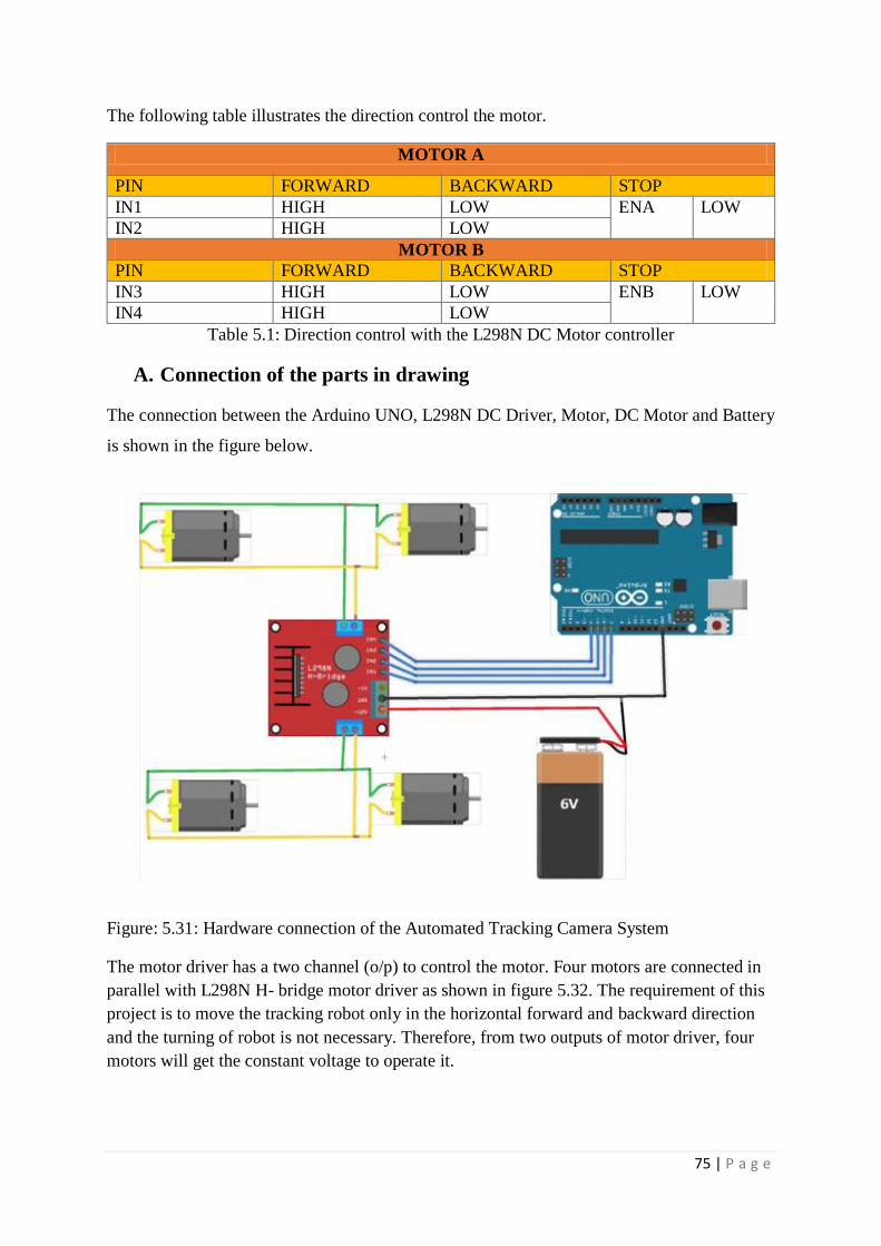
75 | P a g e

The following table illustrates the direction control the motor.

MOTOR A

PIN FORWARD BACKWARD STOP

IN1 HIGH LOW ENA LOW

IN2 HIGH LOW

MOTOR B

PIN FORWARD BACKWARD STOP

IN3 HIGH LOW ENB LOW

IN4 HIGH LOW

Table 5.1: Direction control with the L298N DC Motor controller

A. Connection of the parts in drawing

The connection between the Arduino UNO, L298N DC Driver, Motor, DC Motor and Battery

is shown in the figure below.

Figure: 5.31: Hardware connection of the Automated Tracking Camera System

The motor driver has a two channel (o/p) to control the motor. Four motors are connected in

parallel with L298N H- bridge motor driver as shown in figure 5.32. The requirement of this

project is to move the tracking robot only in the horizontal forward and backward direction

and the turning of robot is not necessary. Therefore, from two outputs of motor driver, four

motors will get the constant voltage to operate it.

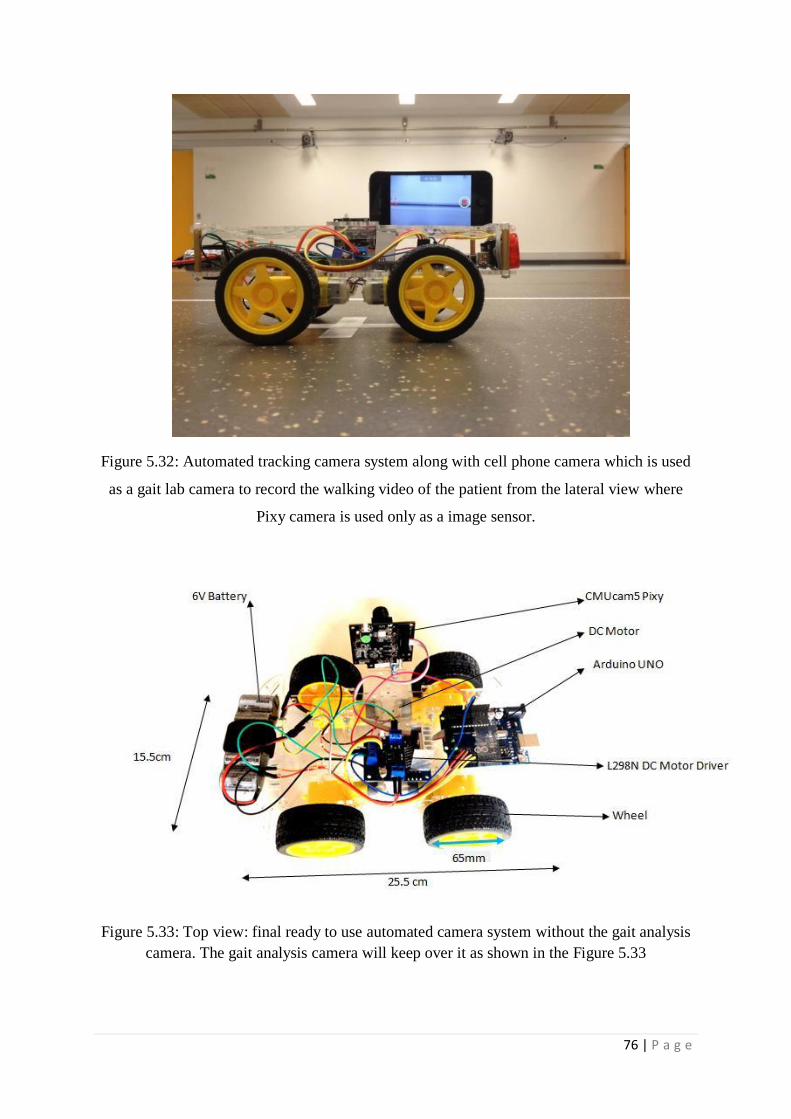
76 | P a g e

Figure 5.32: Automated tracking camera system along with cell phone camera which is used

as a gait lab camera to record the walking video of the patient from the lateral view where

Pixy camera is used only as a image sensor.

Figure 5.33: Top view: final ready to use automated camera system without the gait analysis

camera. The gait analysis camera will keep over it as shown in the Figure 5.33

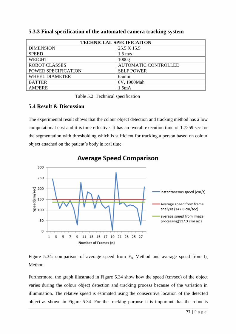
77 | P a g e

5.3.3 Final specification of the automated camera tracking system

TECHNICLAL SPECIFICAITON

DIMENSION 25.5 X 15.5

SPEED 1.5 m/s

WEIGHT 1000g

ROBOT CLASSES AUTOMATIC CONTROLLED

POWER SPECIFICATION SELF POWER

WHEEL DIAMETER 65mm

BATTER 6V, 1900Mah

AMPERE 1.5mA

5.4 Result & Discussion

The experimental result shows that the colour object detection and tracking method has a low

computational cost and it is time effective. It has an overall execution time of 1.7259 sec for

the segmentation with thresholding which is sufficient for tracking a person based on colour

object attached on the patient’s body in real time.

Figure 5.34: comparison of average speed from FA Method and average speed from IA

Method

Furthermore, the graph illustrated in Figure 5.34 show how the speed (cm/sec) of the object

varies during the colour object detection and tracking process because of the variation in

illumination. The relative speed is estimated using the consecutive location of the detected

object as shown in Figure 5.34. For the tracking purpose it is important that the robot is

Table 5.2: Technical specification

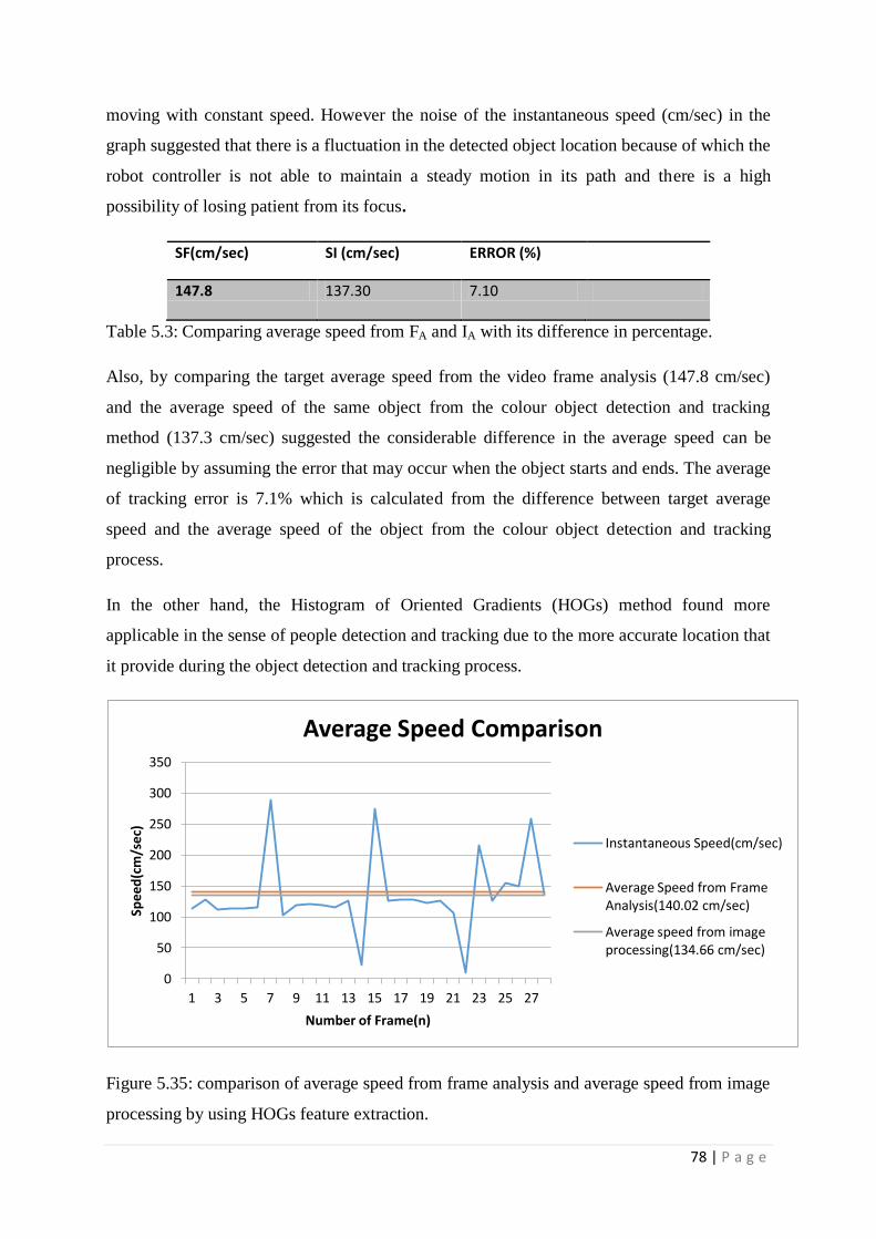
78 | P a g e

moving with constant speed. However the noise of the instantaneous speed (cm/sec) in the

graph suggested that there is a fluctuation in the detected object location because of which the

robot controller is not able to maintain a steady motion in its path and there is a high

possibility of losing patient from its focus.

SF(cm/sec) SI (cm/sec) ERROR (%)

147.8 137.30 7.10

Table 5.3: Comparing average speed from FA and IA with its difference in percentage.

Also, by comparing the target average speed from the video frame analysis (147.8 cm/sec)

and the average speed of the same object from the colour object detection and tracking

method (137.3 cm/sec) suggested the considerable difference in the average speed can be

negligible by assuming the error that may occur when the object starts and ends. The average

of tracking error is 7.1% which is calculated from the difference between target average

speed and the average speed of the object from the colour object detection and tracking

process.

In the other hand, the Histogram of Oriented Gradients (HOGs) method found more

applicable in the sense of people detection and tracking due to the more accurate location that

it provide during the object detection and tracking process.

Figure 5.35: comparison of average speed from frame analysis and average speed from image

processing by using HOGs feature extraction.

0

50

100

150

200

250

300

350

1 3 5 7 9 11 13 15 17 19 21 23 25 27

Spee

d(c

m/s

ec)

Number of Frame(n)

Average Speed Comparison

Instantaneous Speed(cm/sec)

Average Speed from Frame Analysis(140.02 cm/sec)

Average speed from image processing(134.66 cm/sec)

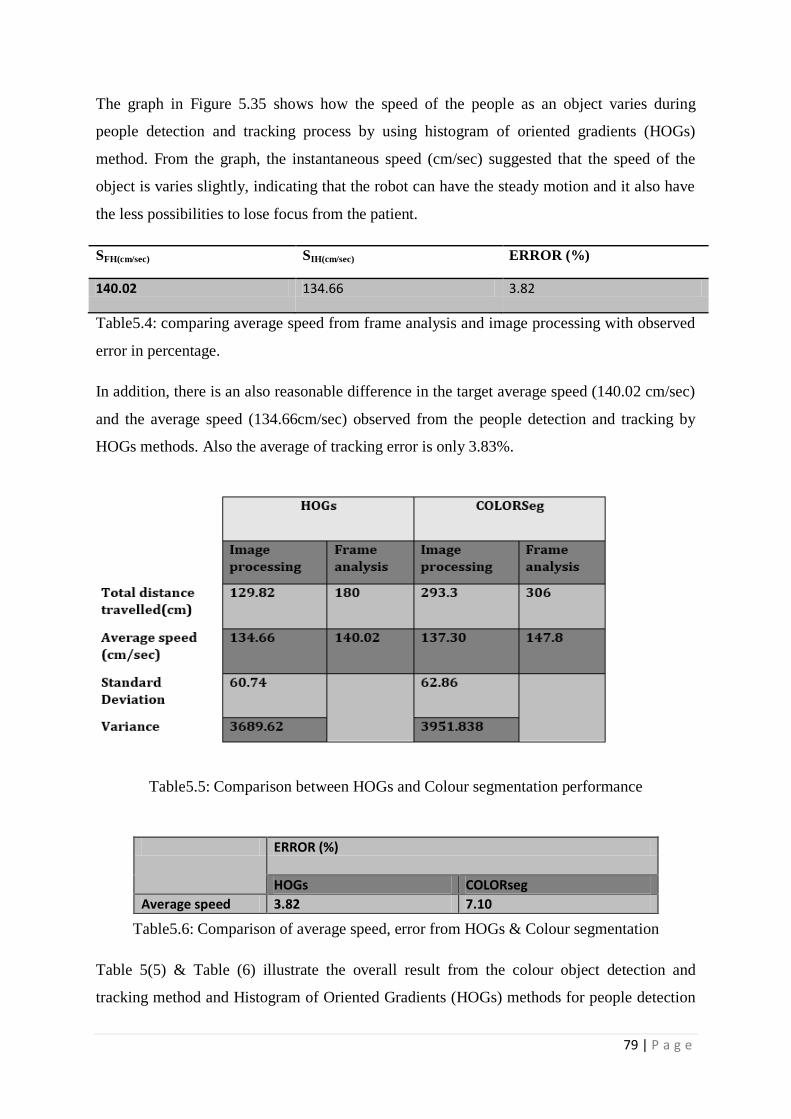
79 | P a g e

The graph in Figure 5.35 shows how the speed of the people as an object varies during

people detection and tracking process by using histogram of oriented gradients (HOGs)

method. From the graph, the instantaneous speed (cm/sec) suggested that the speed of the

object is varies slightly, indicating that the robot can have the steady motion and it also have

the less possibilities to lose focus from the patient.

SFH(cm/sec) SIH(cm/sec) ERROR (%)

140.02 134.66 3.82

Table5.4: comparing average speed from frame analysis and image processing with observed

error in percentage.

In addition, there is an also reasonable difference in the target average speed (140.02 cm/sec)

and the average speed (134.66cm/sec) observed from the people detection and tracking by

HOGs methods. Also the average of tracking error is only 3.83%.

Table5.5: Comparison between HOGs and Colour segmentation performance

Table5.6: Comparison of average speed, error from HOGs & Colour segmentation

Table 5(5) & Table (6) illustrate the overall result from the colour object detection and

tracking method and Histogram of Oriented Gradients (HOGs) methods for people detection

ERROR (%)

HOGs COLORseg

Average speed 3.82 7.10

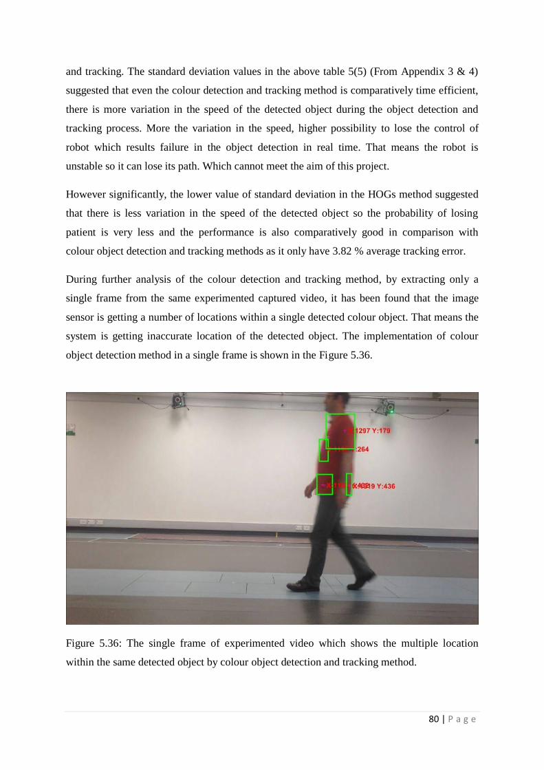
80 | P a g e

and tracking. The standard deviation values in the above table 5(5) (From Appendix 3 & 4)

suggested that even the colour detection and tracking method is comparatively time efficient,

there is more variation in the speed of the detected object during the object detection and

tracking process. More the variation in the speed, higher possibility to lose the control of

robot which results failure in the object detection in real time. That means the robot is

unstable so it can lose its path. Which cannot meet the aim of this project.

However significantly, the lower value of standard deviation in the HOGs method suggested

that there is less variation in the speed of the detected object so the probability of losing

patient is very less and the performance is also comparatively good in comparison with

colour object detection and tracking methods as it only have 3.82 % average tracking error.

During further analysis of the colour detection and tracking method, by extracting only a

single frame from the same experimented captured video, it has been found that the image

sensor is getting a number of locations within a single detected colour object. That means the

system is getting inaccurate location of the detected object. The implementation of colour

object detection method in a single frame is shown in the Figure 5.36.

Figure 5.36: The single frame of experimented video which shows the multiple location

within the same detected object by colour object detection and tracking method.

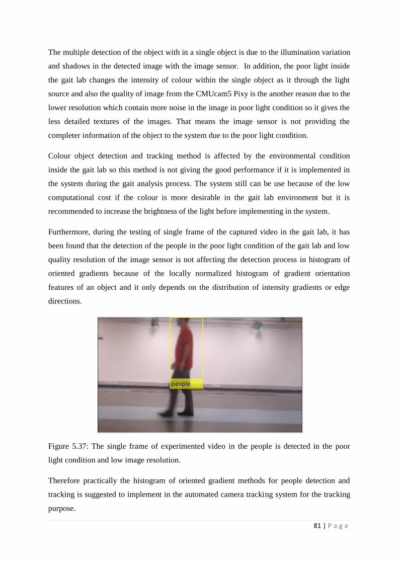
81 | P a g e

The multiple detection of the object with in a single object is due to the illumination variation

and shadows in the detected image with the image sensor. In addition, the poor light inside

the gait lab changes the intensity of colour within the single object as it through the light

source and also the quality of image from the CMUcam5 Pixy is the another reason due to the

lower resolution which contain more noise in the image in poor light condition so it gives the

less detailed textures of the images. That means the image sensor is not providing the

completer information of the object to the system due to the poor light condition.

Colour object detection and tracking method is affected by the environmental condition

inside the gait lab so this method is not giving the good performance if it is implemented in

the system during the gait analysis process. The system still can be use because of the low

computational cost if the colour is more desirable in the gait lab environment but it is

recommended to increase the brightness of the light before implementing in the system.

Furthermore, during the testing of single frame of the captured video in the gait lab, it has

been found that the detection of the people in the poor light condition of the gait lab and low

quality resolution of the image sensor is not affecting the detection process in histogram of

oriented gradients because of the locally normalized histogram of gradient orientation

features of an object and it only depends on the distribution of intensity gradients or edge

directions.

Figure 5.37: The single frame of experimented video in the people is detected in the poor

light condition and low image resolution.

Therefore practically the histogram of oriented gradient methods for people detection and

tracking is suggested to implement in the automated camera tracking system for the tracking

purpose.

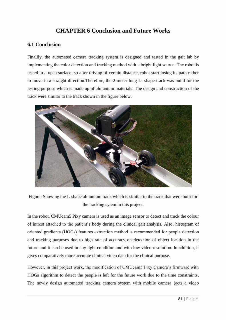
81 | P a g e

CHAPTER 6 Conclusion and Future Works

6.1 Conclusion

Finallly, the automated camera tracking system is designed and tested in the gait lab by

implementing the color detection and tracking method with a bright light source. The robot is

tested in a open surface, so after driving of certain distance, robot start losing its path rather

to move in a straight direction.Therefore, the 2 meter long L- shape track was build for the

testing purpose which is made up of almunium materials. The design and construction of the

track were similar to the track shown in the figure below.

Figure: Showing the L-shape almunium track which is similar to the track that were built for

the tracking sytem in this project.

In the robot, CMUcam5 Pixy camera is used as an image sensor to detect and track the colour

of intrest attached to the patient’s body during the clinical gait analysis. Also, histogram of

oriented gradients (HOGs) features extraction method is recommended for people detection

and tracking purposes due to high rate of accuracy on detection of object location in the

future and it can be used in any light condition and with low video resolution. In addition, it

gives comparatively more accurate clinical video data for the clinical purpose.

However, in this project work, the modification of CMUcam5 Pixy Camera’s firmware with

HOGs algorithm to detect the people is left for the future work due to the time constraints.

The newly design automated tracking camera system with mobile camera (acts a video

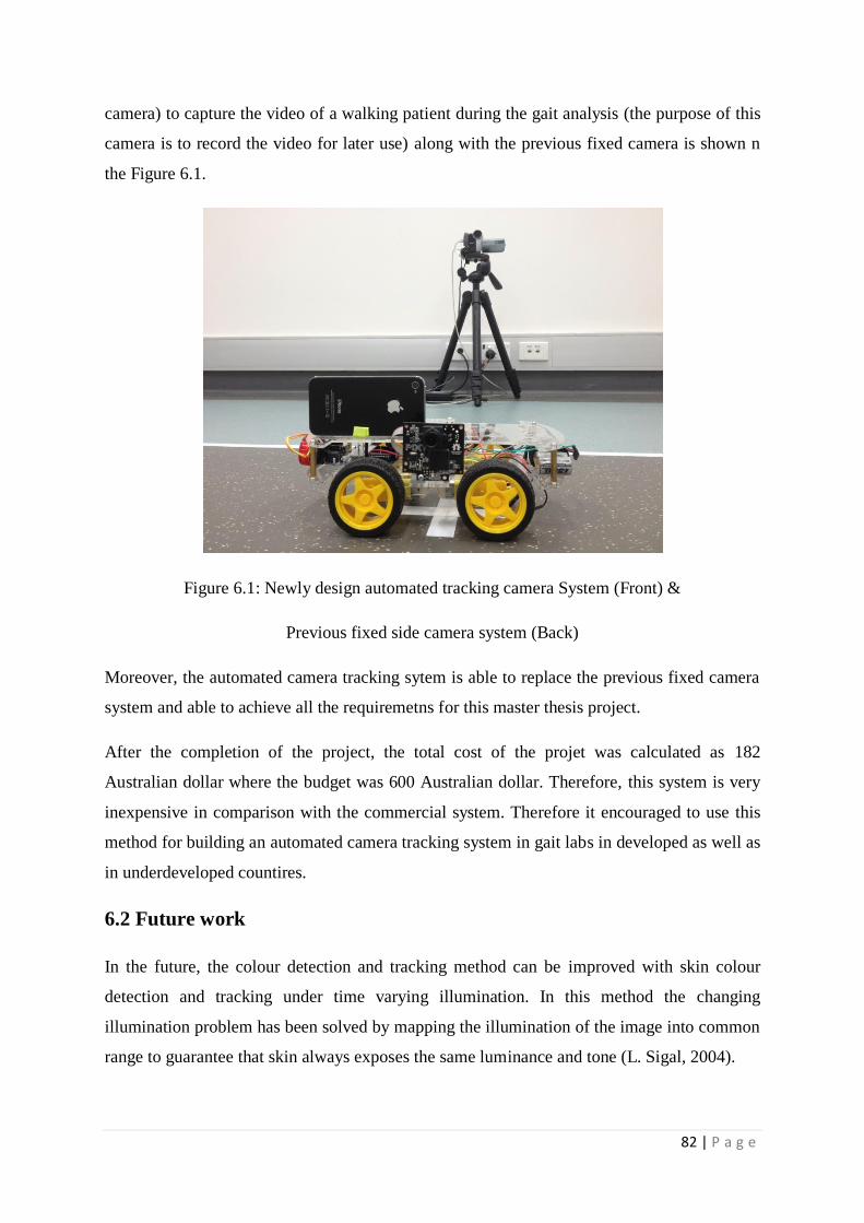
82 | P a g e

camera) to capture the video of a walking patient during the gait analysis (the purpose of this

camera is to record the video for later use) along with the previous fixed camera is shown n

the Figure 6.1.

Figure 6.1: Newly design automated tracking camera System (Front) &

Previous fixed side camera system (Back)

Moreover, the automated camera tracking sytem is able to replace the previous fixed camera

system and able to achieve all the requiremetns for this master thesis project.

After the completion of the project, the total cost of the projet was calculated as 182

Australian dollar where the budget was 600 Australian dollar. Therefore, this system is very

inexpensive in comparison with the commercial system. Therefore it encouraged to use this

method for building an automated camera tracking system in gait labs in developed as well as

in underdeveloped countires.

6.2 Future work

In the future, the colour detection and tracking method can be improved with skin colour

detection and tracking under time varying illumination. In this method the changing

illumination problem has been solved by mapping the illumination of the image into common

range to guarantee that skin always exposes the same luminance and tone (L. Sigal, 2004).

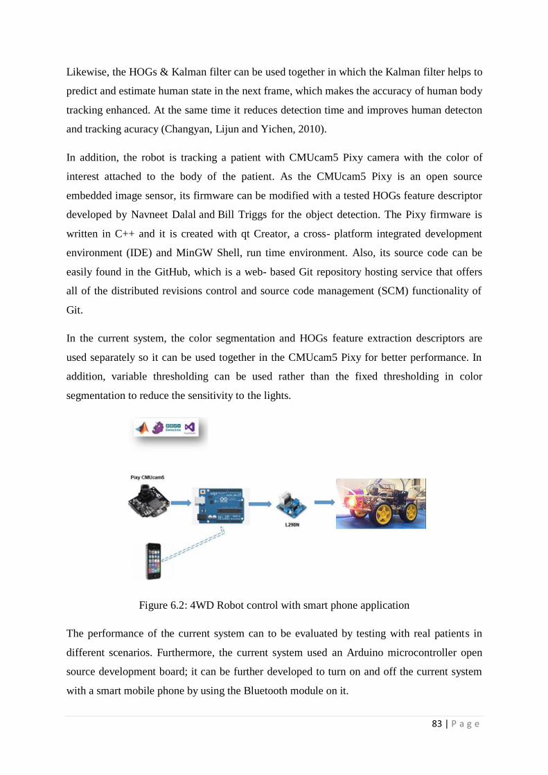
83 | P a g e

Likewise, the HOGs & Kalman filter can be used together in which the Kalman filter helps to

predict and estimate human state in the next frame, which makes the accuracy of human body

tracking enhanced. At the same time it reduces detection time and improves human detecton

and tracking acuracy (Changyan, Lijun and Yichen, 2010).

In addition, the robot is tracking a patient with CMUcam5 Pixy camera with the color of

interest attached to the body of the patient. As the CMUcam5 Pixy is an open source

embedded image sensor, its firmware can be modified with a tested HOGs feature descriptor

developed by Navneet Dalal and Bill Triggs for the object detection. The Pixy firmware is

written in C++ and it is created with qt Creator, a cross- platform integrated development

environment (IDE) and MinGW Shell, run time environment. Also, its source code can be

easily found in the GitHub, which is a web- based Git repository hosting service that offers

all of the distributed revisions control and source code management (SCM) functionality of

Git.

In the current system, the color segmentation and HOGs feature extraction descriptors are

used separately so it can be used together in the CMUcam5 Pixy for better performance. In

addition, variable thresholding can be used rather than the fixed thresholding in color

segmentation to reduce the sensitivity to the lights.

Figure 6.2: 4WD Robot control with smart phone application

The performance of the current system can to be evaluated by testing with real patients in

different scenarios. Furthermore, the current system used an Arduino microcontroller open

source development board; it can be further developed to turn on and off the current system

with a smart mobile phone by using the Bluetooth module on it.

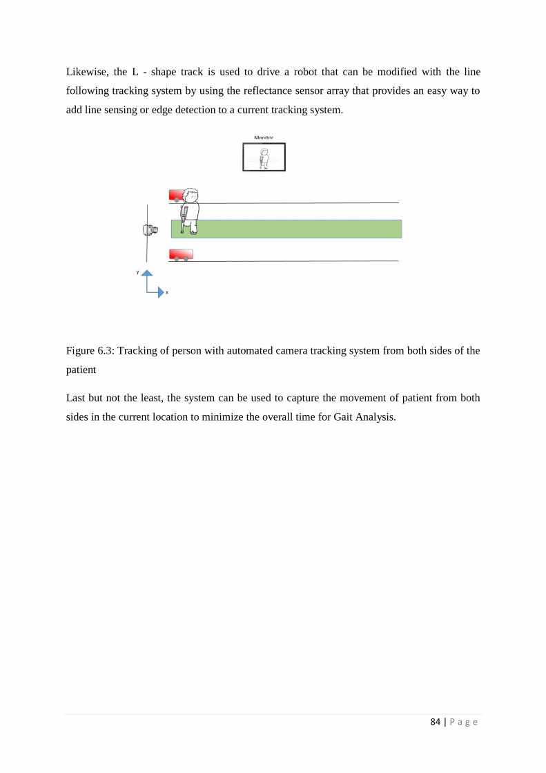
84 | P a g e

Likewise, the L - shape track is used to drive a robot that can be modified with the line

following tracking system by using the reflectance sensor array that provides an easy way to

add line sensing or edge detection to a current tracking system.

Figure 6.3: Tracking of person with automated camera tracking system from both sides of the

patient

Last but not the least, the system can be used to capture the movement of patient from both

sides in the current location to minimize the overall time for Gait Analysis.

REFERENCE

N. Dalal and B. Triggs. Histograms of oriented gradients for human detection. In CVPR,

2005.

Clinicalgaitanalysis.com. (2016). Gait Analysis Models. [online] Available at:

http://www.clinicalgaitanalysis.com/faq/sets/ [Accessed 29 Oct. 2016].

Anon, (2016). Implementation of Hog Edge Detection Algorithm Onfpga's.

L Sigal, S Sclaroff, V Athitsos. Skin color-based video segmentation under time-varying

illumination., IEEE Transactions on Pattern Analysis and Machine Intelligence 26 (7), 862-

877

Changyan, L., Lijun, G. and Yichen, H. (2010). A New Method Combining HOG and

Kalman Filter for Video-based Human Detection and Tracking. 3rd ed., Ningbo University,

Ningbo, China: International Congress on Image and Signal Processing (CISP2010), pp.1-4.

Yi, C., Hong, C. and Hong, S. (2012). IMPROVED SIFT ALGORITHM TO MATCH

POINTS IN THE TEXTURE REGION IMAGE. 1st ed. Thailand: Asian conference on

remote sensing, pp.1-10.

K. Mikolajczyk and C. Schmid, “An affine invariant interest point detector,” in 7th European

Conference on Computer Vision (ECCV 2002), (INRIA Rhone-Alpes GRAVIRCNRS 655,

av. de l’Europe, 38330 Montbonnot, France), pp. 128–142, 2002.

P. Viola and M. J. Jones, “Robust real-time face detection,” International Journal of

Computer Vision, vol. 57, pp. 137–154, 2004. 10.1023/B:VISI.0000013087.49260.fb.

P. Viola and M. Jones, “Rapid object detection using a boosted cascade of simple features,”

Computer Vision and Pattern Recognition, 2001. CVPR 2001. Proceedings of the 2001 IEEE

Computer Society Conference on, vol. 1, pp. I–511 – I–518 vol.1, 2001.

R. Lienhart and J. Maydt, “An extended set of haar-like features for rapid object detection,”

Image Processing. 2002. Proceedings. 2002 International Conference on, vol. 1, pp. I–900 –

I–903 vol.1, 2002.

M. Rudinac and X. Wang, Basic Image Processing for Robotics. Delft University of

Technology.

T. Kadir, A. Zisserman, and M. Brady, “An affine invariant salient region detector,” in

Computer Vision - ECCV 2004 (T. Pajdla and J. Matas, eds.), vol. 3021 of Lecture Notes in

Computer Science, pp. 228–241, Springer Berlin / Heidelberg, 2004.

E. Adelson, C. Anderson, J. Bergen, P. Burt, and J. Ogden, “Pyramid methods in image

processing,” RCA engineer, vol. 29, no. 6, pp. 33–41, 1984.

C. Huijnen, A. Badii, H. Heuvel, P. Caleb-Solly and D. Thiemert, “Maybe it Becomes a

Buddy, but Do Not Call it a Robot” - Seamless Cooperation between Ccompanion Robotics

and Smart Homes, Ambient Intelligence, Volume 7040 of the series Lecture Notes in

Computer Science, pp 324-329, 2011.

Funt, B.V. and Finlayson, G.D. 1995. Color constant color indexing. IEEE Trans. on Pattern

Analysis and Machine Intelligence, 17(5):522-529.

Grimson, E. 1990. Object Recognition by Computer: The Role of Geometric Constraints, The

MIT Press: Cambridge, MA.

Mikolajczyk, K. 2002. Detection of local features invariant to affine transformations, Ph.D.

thesis, Institut National Polytechnique de Grenoble, France.

J. M. S. Belongie and J. Puzicha. Shape matching object recongition using shape contexts.

IEEE Transactions on Pattern Analysis and Machine Intelligence (PAMI), 24(24):509–522,

2002.

D. Lowe. Distinctive image features from scale-invariant keypoints. Internation Journal of

Computer Vision (IJCV), 60(2):91–110, 2004.

P. Viola, M. Jones, and D. Snow. Detecting pedestrians using patterons of motion and

appearance. International Coference on Computer Vision (ICCV), 2003.

D. M. Gavrila. The visual analysis of human movement: A survey. Computer Vision and

Image Understanding (CVIU), 73(1):82.98, 1999.

P. Viola, M. J. Jones, and D. Snow. Detecting pedestrians using patterns of motion and

appearance. The 9th International Conference on Computer Vision (ICCV), Nice, France,

volume 1, pages 734.741, 2003.

Roach, J.W., and Aggarwal, J.K.,

Determining the Movement of Objects from a Sequence of Images,

PAMI(2), No. 6, November 1980, pp. 554-562. Shu, C., Ding, X. and Fang, C. (2011).

Histogram of the oriented gradient for face recognition. Tinshhua Sci. Technol., 16(2),

pp.216-224.

Tracking, C. (2016). Color Object Tracking - File Exchange - MATLAB Central. [online]

Au.mathworks.com. Available at:

http://au.mathworks.com/matlabcentral/fileexchange/52790-color-object-

tracking?s_tid=srchtitle [Accessed 29 May 2016].

Learn.adafruit.com. (2016). Overview and Materials | Pixy Pet Robot - Color vision follower

| Adafruit Learning System. [online] Available at: https://learn.adafruit.com/pixy-pet-robot-

color-vision-follower-using-pixycam/overview [Accessed 29 May 2016].

Au.mathworks.com. (2016). Digit Classification Using HOG Features - MATLAB &

Simulink Example. [online] Available at:

http://au.mathworks.com/help/vision/examples/digit-classification-using-hog-

features.html?s_tid=srchtitle [Accessed 29 May 2016].

Docs.opencv.org. (2016). Harris corner detector — OpenCV 2.4.13.0 documentation

Longuet-Higgins,H.C., A Computer Algorithm for Reconstructing a Scene from Two

Projections,Nature(293), No. 5828, 10 September 1981, pp. 133-135.

L.F. Shampine and P. Gahinet, "Delay-differential-algebraic equations in control

theory," Applied Numerical Mathematics, Vol. 56, Issues 3–4, pp. 574–588.

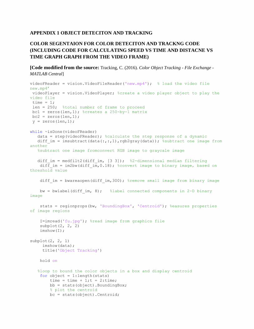
APPENDIX 1 OBJECT DETECITON AND TRACKING

COLOR SEGENTAION FOR COLOR DETECITON AND TRACKNG CODE

(INCLUDING CODE FOR CALCULATING SPEED VS TIME AND DISTACNE VS

TIME GRAPH GRAPH FROM THE VIDEO FRAME)

[Code modified from the source: Tracking, C. (2016). Color Object Tracking - File Exchange -

MATLAB Central]

videoFReader = vision.VideoFileReader('new.mp4'); % load the video file

new.mp4’ videoPlayer = vision.VideoPlayer; %create a video player object to play the

video file time = 1; len = 250; %total number of frame to proceed bc1 = zeros(len,1); %creates a 250-by-1 matrix bc2 = zeros(len,1); y = zeros(len,1);

while ~isDone(videoFReader) data = step(videoFReader); %calculate the step response of a dynamic diff_im = imsubtract(data(:,:,1),rgb2gray(data)); %subtract one image from

another %subtract one image fromconvert RGB image to graycale image

diff_im = medfilt2(diff_im, [3 3]); %2-dimensional median filtering diff_im = im2bw(diff_im,0.18); %convert image to binary image, based on

threshold value

diff_im = bwareaopen(diff_im,300); %remove small image from binary image

bw = bwlabel(diff_im, 8); %label connected components in 2-D binary

image

stats = regionprops(bw, 'BoundingBox', 'Centroid'); %easures properties

of image regions

I=imread('fu.jpg'); %read image from graphics file subplot(2, 2, 2) imshow(I);

subplot(2, 2, 1) imshow(data); title('Object Tracking')

hold on

%loop to bound the color objects in a box and display centroid for object = 1:length(stats) time = time + 1;t = 2:time; bb = stats(object).BoundingBox; % plot the centroid bc = stats(object).Centroid;

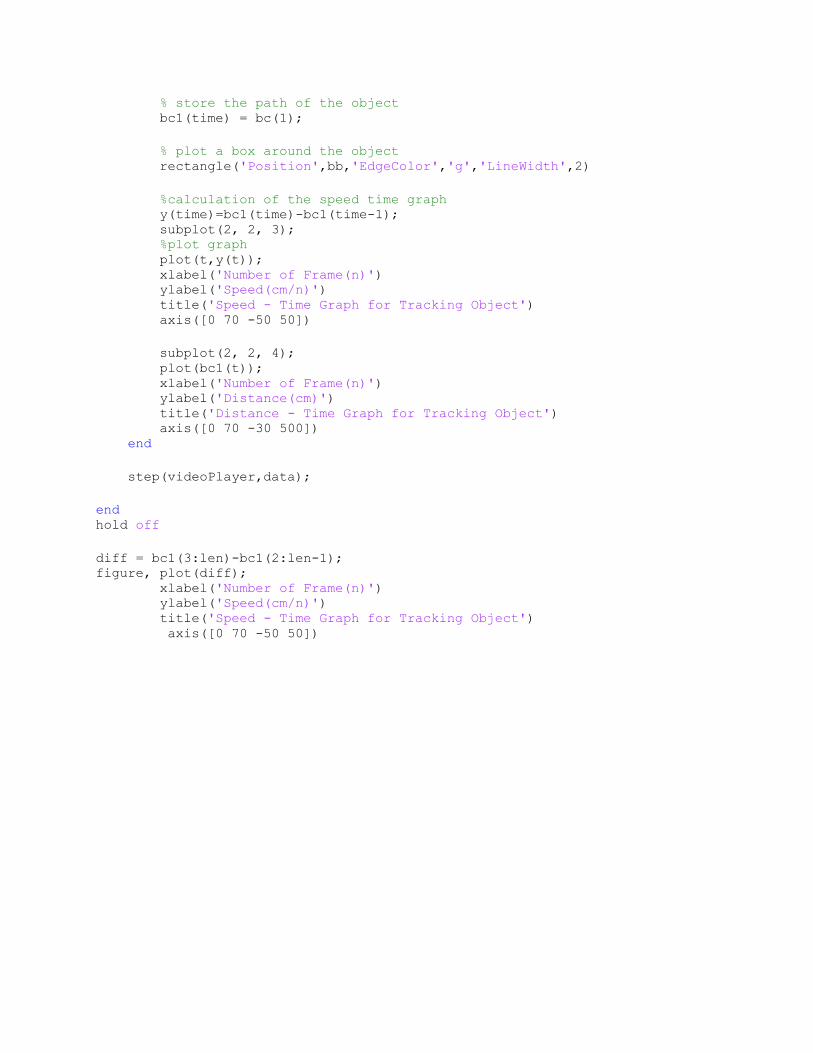
% store the path of the object bc1(time) = bc(1);

% plot a box around the object rectangle('Position',bb,'EdgeColor','g','LineWidth',2)

%calculation of the speed time graph y(time)=bc1(time)-bc1(time-1); subplot(2, 2, 3); %plot graph plot(t,y(t)); xlabel('Number of Frame(n)') ylabel('Speed(cm/n)') title('Speed - Time Graph for Tracking Object') axis([0 70 -50 50])

subplot(2, 2, 4); plot(bc1(t)); xlabel('Number of Frame(n)') ylabel('Distance(cm)') title('Distance - Time Graph for Tracking Object') axis([0 70 -30 500]) end

step(videoPlayer,data);

end hold off

diff = bc1(3:len)-bc1(2:len-1); figure, plot(diff); xlabel('Number of Frame(n)') ylabel('Speed(cm/n)') title('Speed - Time Graph for Tracking Object') axis([0 70 -50 50])

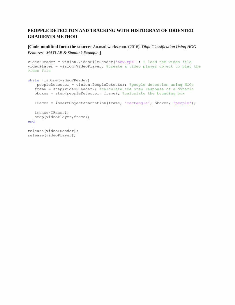
PEOPPLE DETECITON AND TRACKING WITH HISTOGRAM OF ORIENTED

GRADIENTS METHOD

[Code modified form the source: Au.mathworks.com. (2016). Digit Classification Using HOG

Features - MATLAB & Simulink Example.]

videoFReader = vision.VideoFileReader('new.mp4'); % load the video file videoPlayer = vision.VideoPlayer; %create a video player object to play the

video file

while ~isDone(videoFReader) peopleDetector = vision.PeopleDetector; %people detection using HOGs frame = step(videoFReader); %calculate the step response of a dynamic bboxes = step(peopleDetector, frame); %calculate the bounding box

IFaces = insertObjectAnnotation(frame, 'rectangle', bboxes, 'people');

imshow(IFaces); step(videoPlayer,frame); end

release(videoFReader); release(videoPlayer);

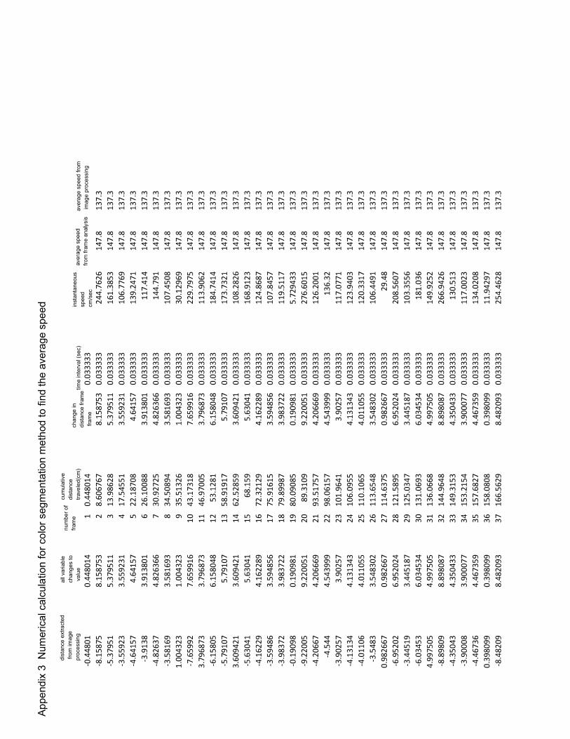
DIS

TA

NC

ET

RA

VE

L

dis

tanc

ee

xtra

cte

d f

rom

ima

gep

roce

ssin

g

all

vari

able

cha

nge

sto

va

lue

nu

mb

er

of

fram

e

cum

ula

tive

dis

tanc

etr

ave

led

(cm

)ch

ang

ein

dis

tanc

efr

ame

fra

me

time

inte

rva

l(se

c)in

sta

nta

ne

ous

spe

edcm

/sec

ave

rag

esp

eed

from

imag

e p

roce

ssin

g

Ap

pend

ix3

Num

eric

alca

lcu

latio

nfo

rco

lor

seg

me

ntat

ion

met

hod

tofin

dth

eav

era

gesp

eed

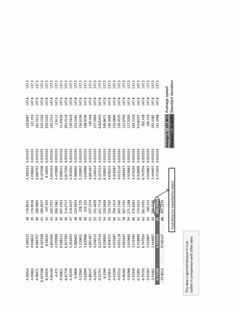
Ave

rage

spee

dS

tand

ard

devi

atio

n

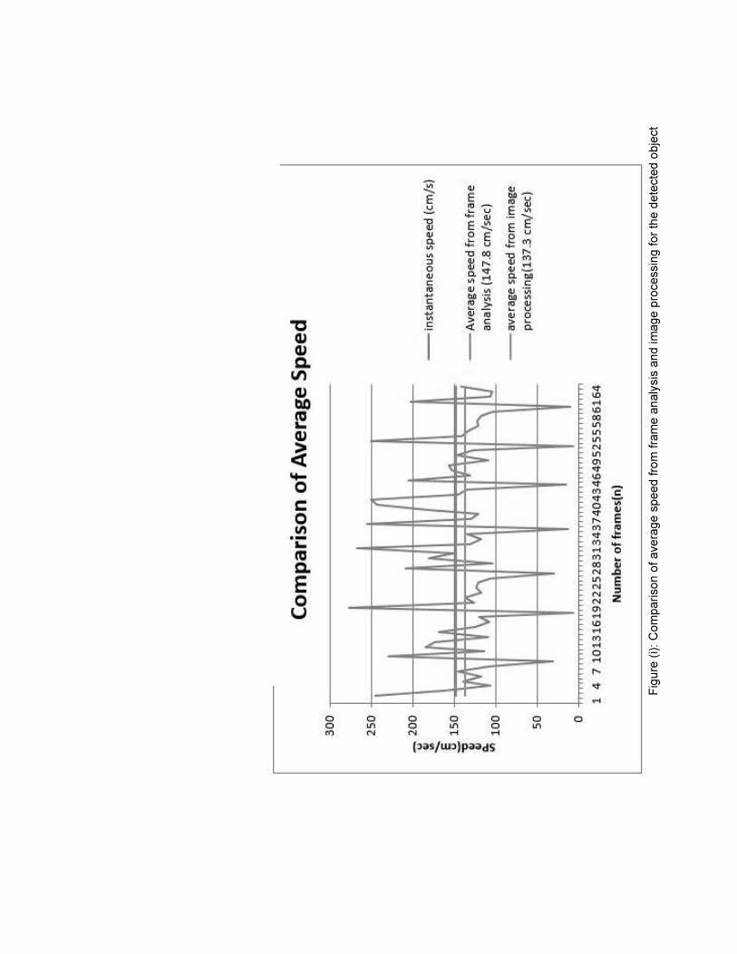
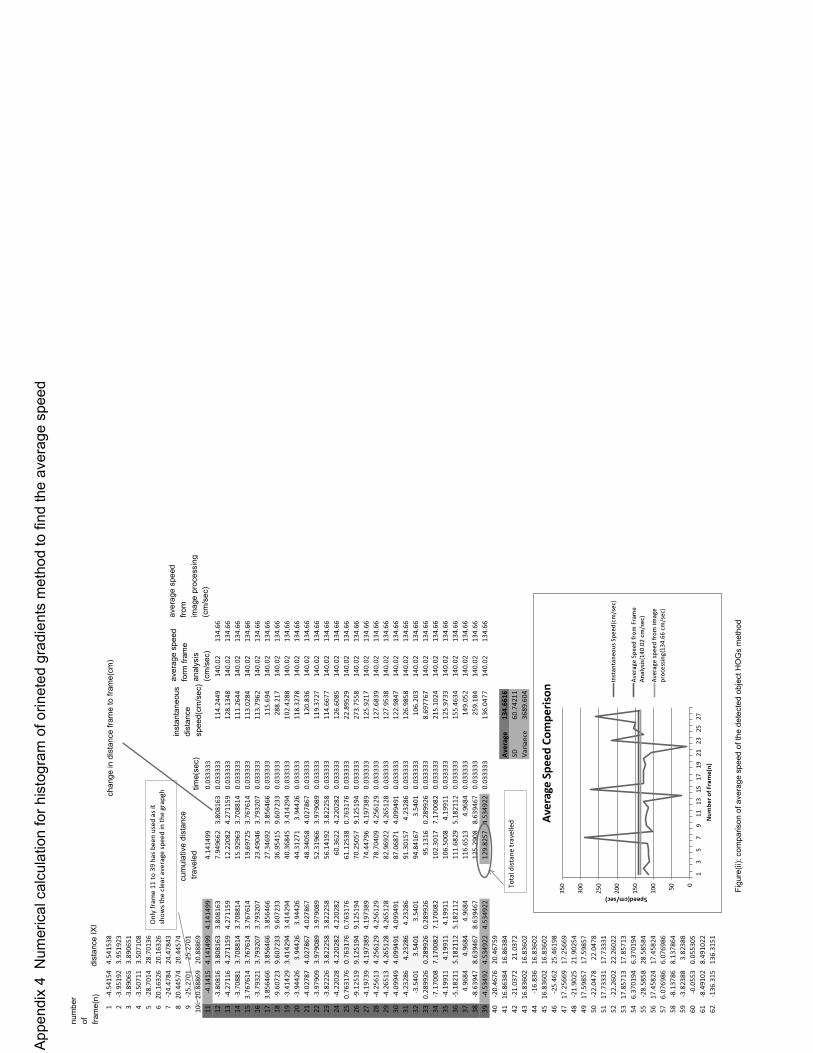
nu

mb

er

of

fram

e(n

)d

ista

nce

IXI

cum

ula

tive

dis

tanc

e t

rave

led

cha

nge

ind

ista

nce

fram

eto

fram

e(c

m)

time(

sec)

inst

ant

an

eou

sd

ista

nce

spe

ed(c

m/s

ec)

ave

rag

esp

eed

form

fram

e

an

alys

is(c

m/s

ec)

ave

rag

esp

eed

from

ima

gep

roce

ssin

g(c

m/s

ec)

Fig

ure

(ii):

com

pa

riso

no

fa

vera

ge

spe

edo

fth

ed

ete

cte

do

bje

ctH

OG

sm

eth

od

Ap

pend

ix4

Num

eric

alc

alcu

latio

nfo

rh

isto

gra

mof

orin

ete

dg

radi

ent

sm

eth

od

tofin

dth

ea

vera

ge

spee

d

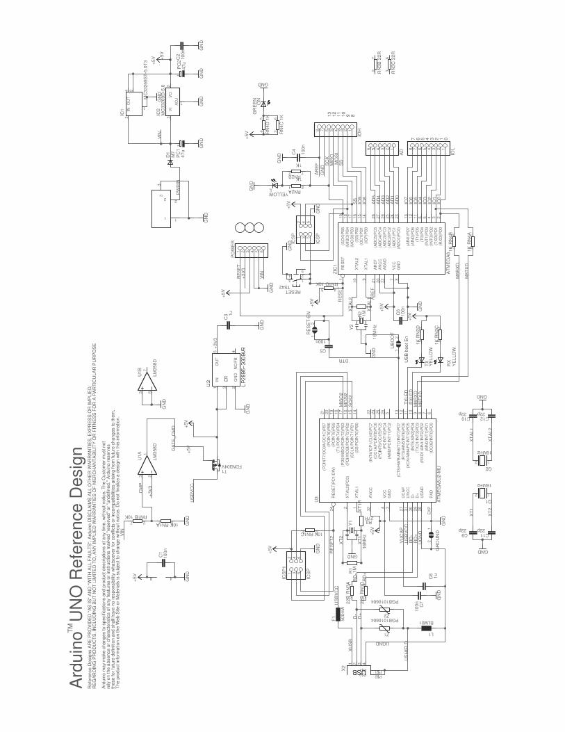
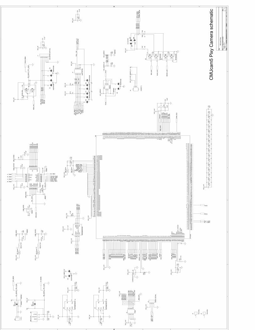
CM

Uca

m5

Pix

yC

amer

asc

hem

atic

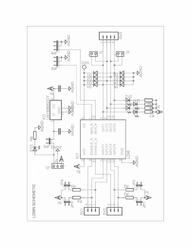
L29

8NS

CH

EM

ET

IC