Weyl, Dirac and Maxwell Quantum Cellular Automata:analitical solutions and phenomenological predictions of the Quantum Cellular

Automata Theory of Free Fields∗

Alessandro Bisio,† Giacomo Mauro D’Ariano,‡ Paolo Perinotti,§ and Alessandro Tosini§

QUIT group, Dipartimento di Fisica, Universita degli Studi di Pavia, via Bassi 6, 27100 Pavia, Italy andIstituto Nazionale di Fisica Nucleare, Gruppo IV, via Bassi 6, 27100 Pavia, Italy

Recent advances on quantum foundations achieved the derivation of free quantum field theoryfrom general principles, without referring to mechanical notions and relativistic invariance. Fromthe aforementioned principles a quantum cellular automata (QCA) theory follows, whose relativisticlimit of small wave-vector provides the free dynamics of quantum field theory. The QCA theory canbe regarded as an extended quantum field theory that describes in a unified way all scales rangingfrom an hypothetical discrete Planck scale up to the usual Fermi scale.

The present paper reviews the elementary automaton theory for the Weyl field, and the compositeautomata for Dirac and Maxwell fields. We then give a simple analysis of the dynamics in themomentum space in terms of a dispersive differential equation for narrowband wave-packets, andsome account on the position space description in terms of a discrete path-integral approach. Wethen review the phenomenology of the free-field automaton and consider possible visible effectsarising from the discreteness of the framework. We conclude introducing the consequences of theautomaton distorted dispersion relation, leading to a deformed Lorentz covariance and to possibleeffects on the thermodynamics of ideal gases.

I. INTRODUCTION

The notion of cellular automaton was introduced by J. von Neumann in his seminal paper [2] where he aimedat modeling a self-reproducing entity. The idea behind the concept of a cellular automaton is that the richness ofstates exhibited by the evolution of a macroscopic system could emerge from a simple local interaction rule amongits elementary constituents. More precisely, a cellular automaton is a lattice of cells that can be in a finite numberof states, together with a rule for the update of cell states from time t to time t + 1. The principal requirement forsuch rule is locality : The state of the cell x at step t+ 1 depends on the states of a finite number of neighboring cellsat step t. The use of classical cellular automata for simulation of quantum mechanics was proposed by ’tHooft [3],followed by other authors [4].

The first author to suggest the introduction of the quantum version of cellular automata was R. Feynman in thecelebrated paper of Ref. [5]. Since then, the interest in quantum cellular automata (QCAs), has been rapidly growing,especially in the Quantum Information community, leading to many results about their general structure (see e.gRefs.[6–8] and references therein). Special attention is devoted in the literature to QCAs with linear evolution, knownas Quantum Walks (QWs) [9–12], which were especially applied in the design of quantum algorithms [13–16], providinga speedup for relevant computational problems.

More recently QCAs have been considered as a new mathematical framework for Quantum Field Theory [17–25].Within this approach, each cell of the lattice corresponds to the evaluation ψ(x) of a quantum field at the site x ofa lattice, with the dynamics updated in discrete time steps by a local unitary evolution. Assuming that the latticespacing corresponds to an hypothetical discrete Planck scale[70], the usual quantum field evolution should emergeas a large scale approximation of the automaton dynamics. On the other hand, the QCA dynamics will exhibit adifferent behaviour at a very small scale, corresponding to ultra-relativistic wave-vectors.

The analysis of this new phenomenology is of crucial importance in providing the first step towards an experimentaltest of the theory as well as a valuable insight on the distinctive features of the QCA theory. Until now the researchwas mainly focused on linear QCAs which describe the dynamics of free field. By means of a Fourier transform thelinear dynamics can be easily integrated and then, as we will show in section III A, an approximated model for the

∗ Work presented (together with Ref.[1]) at the conference Quantum Theory: from Problems to Advances, held on 9-12 June 2014 at atLinnaeus University, Vaxjo University, Sweden.

†alessandro.bisio@unipv.it‡dariano@unipv.it§paolo.perinotti@unipv.it

arX

iv:1

601.

0484

2v1

[qu

ant-

ph]

19

Jan

2016

2

evolution of particle states (i.e. state of the dynamics narrow-band in wave-vector) can be obtained. Moreover, itis also possible to derive an analytical solution of the evolution in terms of a path sum in the position space, thusgiving the QCA analog of the Feynman propagator [26, 27]. In section IV we will exploit these tools to explore manydynamical features of the QCA models for the Weyl and Dirac fields and to compare them with the correspondingcounterpart emerging from the Weyl and Dirac Equation. We will see that, when considering massive Fermionicfields (e.g electrons) the deviations from the usual field dynamics cannot be reached by present day experiments,contrarily to the case of the QCA theory of the free electromagnetic field. In section IV D we will review the mainphenomenological aspects of the QCA model for free photons (that in this framework become composite particles) withspecial emphasis of the emergence of a frequency-dependent speed of light, a Planck-scale effect already considered byother authors in the Quantum Gravity community [28–32]. In the final Section of this paper we address two issues ofthe QCA theory that are still under investigation. The first one concerns the notion of Lorentz covariance: Becauseof its intrinsic discreteness, a QCA model cannot enjoy a notion of Lorentzian space-time and the usual Lorentzcovariance must break down at very small distances. One way of addressing the problem of changing the referenceframe is to assume that every inertial observer must observe the same dynamics. Then one can look for a set ofmodified Lorentz transformtion which keep the QCA dispersion relation invariant. The first step of this analysis arereported in Section V A. The second issue we will briefly address in Section V B are thermodynamical effects thatcould emerge from modified QCA dynamics.

II. WEYL, DIRAC AND MAXWELL AUTOMATA

A Quantum Cellular Automaton (QCA) describes the discrete time evolution of a set of cells, each one containingan array of quantum modes. In this section we review the QCA models for the free fermions and for the freeelectromagnetic field. For a complete presentation of these results we refer to Refs. [19–21]. Within our frameworkwe will consider Fermionic fields, our choice being motivated by the requirement that amount of information in finitenumber of cells must be finite. Then, each cell x of the lattice is associated with the Fermionic algebra generatedby the field operators {ψ(x), ψ†(x)} which obey the canonical anticommutation relation [ψ(x), ψ†(x′)]+ = δx,x′ and[ψ(x), ψ(x′)]+ = 0 [71]. With a slight genealization, we consider the case in which each cell correspond to morethan one Fermionic mode. Different Fermionic modes will be denoted by an additional label, e.g. ψi(x). Theautomaton evolution will be specified by providing the unit-step update of the Fermionic field operators. This ruledefines the primitive physical law, and must then be as simple and universal as possible. This principle translatesinto a minimization of the amount of mathematical parameters specifying the evolution. In particular we constrainthe automaton to describe a unitary evolution which is linear in the field. We notice that the linearity of the QCArestrict the scenario to non-interacting field dynamics. Then we require the evolution to be local, which means thatat each step every cell interacts with a finite number of neighboring cells, and homogeneous, meaning that all thesteps are the same, all the cells are identical systems and the interactions with neigbours is the same for each cell(hence also the number of neigbours, and the number of Fermionic modes in each cell). The neighboring notion alsonaturally defines a graph Γ with x as vertices and the neighboring couples as edges. We also assume transitivity, i.e.that every two cells are connected by a path of neighbors and isotropy which means that the neighboring relation ossymmetric and there exist a group of automorphisms for the graph under which the automaton is covariant. Fromthese assumptions one can show[72] that graph Γ is a Cayley graph of a group G. In the following, we consider theAbelian case G = Z3.

Let S+ denote the set of generators of Z3 corresponding to the Cayley graph Γ and let S− be the set of inversegenerators. For a given cell x the set of neighboring cells is given by the set Nx := {x + z | z ∈ S := S+ ∪ S−}, wherewe used the additive notation for the group composition. If s is the number of Fermionic modes in each cell, the singlestep evolution can then be represented in terms of s× s transition matrices Az as follows

ψ(x, t+ 1) =∑z∈S

Azψ(x + z, t). (1)

where ψ(x, t) is the array of field operators at x at step t. Upon introducing the Hilbert space `2(Z3), the automatonevolution can be described by the unitary matrix A on `2(Z3)⊗ Cs given by

A :=∑z∈S

Tz ⊗Az, (2)

where Tx denotes the unitary representation of Z3 on `2(Z3), Ty|x〉 = |x+y〉. If s = 1 , i.e. there only one Fermionicmode in each cell, one can prove that the only evolution which obeys our set of assumptions is the trivial one (A is theidentity matrix). Then we are led to consider the s = 2 case and we denote the two Fermionic modes as ψL(x, t) and

3

ψR(x, t). Moreover in the s = 2 case one can show that our assumptions[73] imply that the only lattice which admitsa nontrivial evolution is the body centered cubic (BCC) one. Being Z3 an abelian group, the Fourier transform iswell defined and the operator A can be block-diagonalized as follows

A =

∫B

d3k |k〉〈k| ⊗Ak, (3)

where |k〉 := (2π)−32∑

x∈Z3 eik·x|x〉, B is the first Brillouin zone of the BCC lattice and Ak :=∑

z∈S k e−ik·zAz is a

2 × 2 unitary for every k. We have only two (up to a local change of basis) non trivial QCAs corresponding to theunitary matrices

A±k := d±k I + n±k · σ = exp[−in±k · σ], (4)

where σ is the array (σx, σy, σz) of Pauli matrices and we defined

n±k :=

sxcycz ∓ cxsysz∓cxsycz − sxcyszcxcysz ∓ sxsycz

, n±k :=λ±k n

±k

sinλ±k,

d±k := (cxcycz ± sxsysz), λ±k := arccos(d±k ),

cα := cos(kα/√

3), sα := sin(kα/√

3), α = x, y, z.

The matrices A±k in Eq. (4) describe the evolution of a two-component Fermionic field,

ψ(k, t+ 1) = A±k ψ(k, t), ψ(k, t) :=

(ψR(k, t)ψL(k, t)

). (5)

The adimensional framework of the automaton corresponds to measure everything in Planck units. In such a case thelimit |k| � 1 corresponds to the relativistic limit, where on has

n±(k) ∼ k√3, A±k ∼ exp[−i k√

3· σ], (6)

corresponding to the Weyl’s evolution, with the rescaling k√3→ k. Since the QCAs A+ and A− reproduce the

dynamics of the Weyl equation in the limit |k| � 1, we refer to them as Weyl automata. For sake of simplicity, inthe following we will consider only one Weyl automaton, i.e. we define Ak := A−k and we similarly drop all the others± superscripts. This choice is completely painless since all the methods that we will use can be easily adapted tothe choice Ak = A−k . However the two automata, beside giving the Weyl equation for small k, exhibit a differentbehaviour at high k and we will point out those differences whenever it will be relevant.

The derivation that we sketch previously can be carried on also in the two dimensional case (considering QCA onCayley graphs of Z2) and in the one dimensional case (considering QCA on Cayley graphs of Z). In the 2-dimensionalcase we obtain a unique (up to a local change of basis) the QCA on the square latticeand it leads to

A(2D)k = IdAk − iσ · aAk , (7)

where the functions ak and dk are expressed in terms of kx := k1+k2√2

and ky := k1−k2√2

as (aAk )x := sxcy, (aAk )y := cxsy,

(aAk )z := sxsy, dAk := cxcy. where ci = cos ki√2

and si = sin ki√2. In the one dimensional case we find

A(1D)k =

(e−ik 0

0 eik

)(8)

Both in the 2-dimensional and 1-dimensional cases the limit |k| � 1 gives the 2-dimensional and 1-dimensional Weylequation respectively (in the 2-dimensional we need the rescaling with the rescaling k√

2→ k.). The QCA in Eqs.

(4, (7) and (8)) describe the dynamics of free massless Fermionic fields. If we couple two Weyl automata Ak with amass term we obtain a new QCA Uk given by

Uk =

(nAk imI

imI nA†k

)n2 +m2 = 1. (9)

4

Clearly this construction can be done in the 1,2 and 3-dimensional cases and the resulting QCA is alway unitary andlocal. One can easily see that in the limit |k| � 1 and m � 1 Eq. 9 (with the appropriate rescaling of k in 2 and 3dimensions) gives the same evolution as Dirac equation and then we denote the automata of Eq. (9) Dirac automata.

The 3-dimensional Weyl QCA can also be use as a building block for QCA model of free electrodynamics. The basicidea is to interpret the photon as a pair of Weyl fermions that are suitably correlated in wave-vector. Then one canshow that, in an appropriate regime, this field obeys the dynamics dictated by the Maxwell equations and the bosoniccommutation relation are recovered. This approach recall the so-called beutrino theory of light of De Broglie [33–37]which suggested that the photon could be a composite particle made of of a neutrino-antineutrino pair. Within ourframework (we omit the details of this construction that can be found in Ref. [21]) the electric and magnetic field aregiven by

E := |nk2

|(FT + F†T ), B := i|nk2

|(F†T − FT ), (10)

2|nk2

|FT = E + iB

FT (k) := F(k)−(

n k2

|n k2| · F(k)

)n k

2

|n k2|

F(k) := (F 1(k), F 2(k), F 3(k))T ,

F j(k) :=

∫dq

(2π)3fk(q)φ

(k2 − q

)σjψ

(k2 + q

)where

∫dq

(2π)3 |fk(q)|2 = 1,∀k and φ (k), ψ (k) are two massless Fermionic fields whose evolution is dictated by the

automaton A∗k and Ak respectively[74], i.e.

φ (k, t) = A∗tk φ (k) ψ (k, t) = Atkφ (k)

φ (k) =

(φR (k)φL (k)

)ψ (k) =

(ψR (k)ψL (k)

).

For an appropriate choice of the functions fk(q) (see Ref. [21]), one can prove that the evolution of the Electric andMagnetic fields which are defined in Eq.(10) is given by the following equations[75]

∂tFT (k, t) = 2n k2× FT (k, t)

2n k2· FT (k, t) = 0,

(11)

which in the limits |k| � 1 and with the rescaling k√3→ k become the Fourier trasform of the usual vacuum Maxwell

equations in position space

∇ ·E = 0 ∇ ·B = 0∂tE = c∇×B ∂tB = −c∇×E .

(12)

Because of this result, we refer to the construcion of Eq. (10) as the Maxwell automaton. This is a slight abuse ofnotation since Eq. (10) does not introduce any new QCA model but it defines a field of bilinear operators, each oneof them evolving with the Weyl automaton, that can be interpreted as the electromagnetic field in vacuum. In thissense the expression “Maxwell automaton” actually means QCA model for the Maxwell equations (in vacuum).

III. ANALYSIS OF THE DYNAMICS

The aim of this section is to analyse the dynamics of the QCA models presented in the previous section. Thematerial of this section can be found in Refs. [19, 20, 26, 27, 38].

In this section we fosus on the single particle sector of the QCA. Since the QCAs we are considering are linear inthe fields the single particle sector contains all the information of the dynamics (it is a free theory). We can thenwrite |ψ(t)〉 = At|ψ(0)〉 where |ψ(t)〉 :=

∑x |ψ(x, t)〉|x〉 is generic one particle state. This kind of framework is better

known in the literature under the name Quantum Walk [9–11, 39–41].

5

A. Interpolating Hamiltonian and differential equation for single-particle wave-packets

Since a QCA (and a Quantum Walk) describes a discrete evolution on a lattice, the notion of Hamiltonian (likeany other differential operators) is completely deprived of physical meaning. However it is useful to introduce aHamiltonian operator Hk, that we call interpolating Hamiltonian that obeys the following equation

Atk = eitHk . (13)

where Atk is defined for any real value of t (the automaton Ak can be any of the QCA models of Section II). It is clearthat Hk is the genrator of the continuous time evolution which interpolate the QCA dynamics between the integersteps. The eigenvalue of Hk have the same modulus and its analytical expression, denoted by ω(k), is the dispersiverelation of the automaton and it provides a lot of information about the dynamics. In analogy with what we doin Quantum Field Theory, states of the dynamics corresponding to the positive eigenvalue ω(k) are called particlestates while eigenstate with negative eigenvalue −ω(k) are called antiparticle states. If we denote with |u〉k a positivefrequency eigenstate of Hk (i.e. Hk|u〉k = ω(k)|u〉k) a generic particle state with positive frequency

|ψ〉+ =

∫dk

(2π)ng(k)|u〉k|k〉 (14)

where n is the dimension of the lattice and g(k) is a normalized probability amplitude. We remind that for the 2 and3-dimensional Dirac QCA Hk has dimension 4 and then both the eigenvalues have degeneracy (corresponding to thespin degree of freedom). The construction of Eq. (14) can be straightforwardly applied also for the definition generalantiparticle states with negative frequency |ψ〉−.

One can use the interpolating Hamiltonian Hk in order to rephrase the continuous evolution in terms of a differentialEquation, i.e.

i∂t|ψ(k, t)〉 = Hk|ψ(k, t)〉. (15)

where |ψ(k, t)〉 is the wave-vector representation of a one-particle state, i.e. |ψ〉 =∫

dk(2π)3 |ψ(k, t)〉|k〉 . When the

initial state has positive frequency (see Eq. (14)) and its distribution g(k) is smoothly peaked around a given k0, theevolution of Eq. (15) can be approximated by the following dispersive equation

i∂tg(x, t) = ±[v · ∇+ 12D · ∇∇]g(x, t), (16)

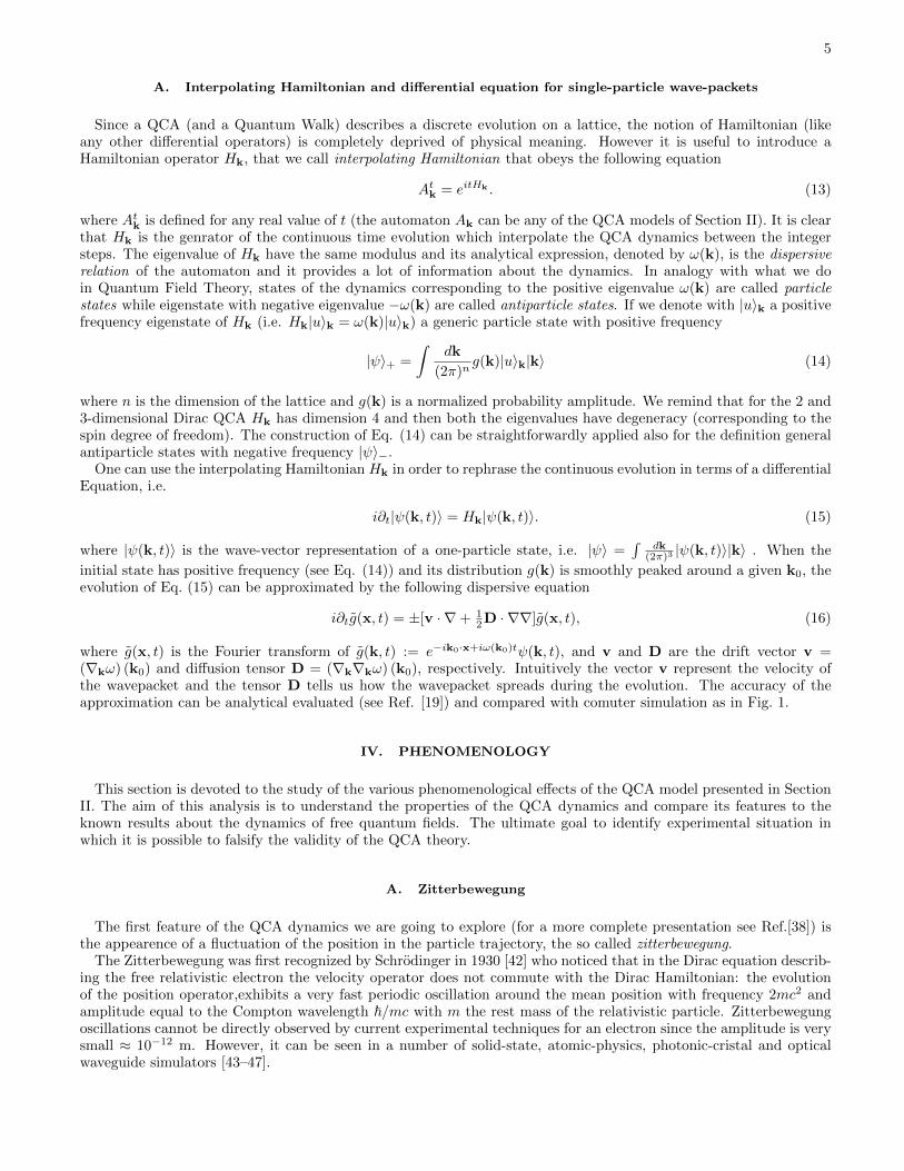
where g(x, t) is the Fourier transform of g(k, t) := e−ik0·x+iω(k0)tψ(k, t), and v and D are the drift vector v =(∇kω) (k0) and diffusion tensor D = (∇k∇kω) (k0), respectively. Intuitively the vector v represent the velocity ofthe wavepacket and the tensor D tells us how the wavepacket spreads during the evolution. The accuracy of theapproximation can be analytical evaluated (see Ref. [19]) and compared with comuter simulation as in Fig. 1.

IV. PHENOMENOLOGY

This section is devoted to the study of the various phenomenological effects of the QCA model presented in SectionII. The aim of this analysis is to understand the properties of the QCA dynamics and compare its features to theknown results about the dynamics of free quantum fields. The ultimate goal to identify experimental situation inwhich it is possible to falsify the validity of the QCA theory.

A. Zitterbewegung

The first feature of the QCA dynamics we are going to explore (for a more complete presentation see Ref.[38]) isthe appearence of a fluctuation of the position in the particle trajectory, the so called zitterbewegung.

The Zitterbewegung was first recognized by Schrodinger in 1930 [42] who noticed that in the Dirac equation describ-ing the free relativistic electron the velocity operator does not commute with the Dirac Hamiltonian: the evolutionof the position operator,exhibits a very fast periodic oscillation around the mean position with frequency 2mc2 andamplitude equal to the Compton wavelength ~/mc with m the rest mass of the relativistic particle. Zitterbewegungoscillations cannot be directly observed by current experimental techniques for an electron since the amplitude is verysmall ≈ 10−12 m. However, it can be seen in a number of solid-state, atomic-physics, photonic-cristal and opticalwaveguide simulators [43–47].

6

t = 0Xx\ = 200

0 200 400 600 8000.000

0.005

0.010

0.015

x

pHxL

t = 0Xx\ = 200

0 100 200 300 400 500 6000.000

0.005

0.010

0.015

0.020

0.025

x

pHxL

t = 200Xx\ = 346

0 200 400 600 8000.000

0.005

0.010

0.015

x

pHxL

t = 200Xx\ = 259

0 100 200 300 400 500 6000.000

0.005

0.010

0.015

0.020

0.025

xpH

xL

t = 600Xx\ = 639

0 200 400 600 8000.000

0.005

0.010

0.015

x

pHxL

t = 600Xx\ = 378

0 100 200 300 400 500 6000.000

0.005

0.010

0.015

0.020

0.025

x

pHxL

FIG. 1: (Colors online) Test of the approximated evolution of Eq. (16) of the one dimensional Dirac automaton evolution.Left figure: here the state is a superposition of Hermite functions (the polynomials Hj(x) multiplied by the Gaussian) peakedaround k0 = 3π/10. Right figure: here the initial state is Gaussian profile peaked around k0 = 0.1. This figure is publishedin Ref. [19].

Here we focus on the one-dimensional Dirac QCA whose epression, introduced in Section II, is easily obtained asspecial case of Eq. (9)[76]

U =

∫ π

−πdk|k〉〈k| ⊗ Uk Uk =

(ne−ik imim neik

)(17)

The “position” operator X corresponding to the representation |x〉 (i.e. such that X|s〉|x〉 = x|s〉|x〉, x ∈ Z) is definedas follows

X =∑x∈Z

x(I ⊗ |x〉〈x|). (18)

and it provides the average location of a wavepacket in terms of 〈ψ|X|ψ〉. If we write the single particle in terms of itspositive frequency and negative frequency components, i.e. |ψ〉 = c+|ψ〉+ + c−|ψ〉−, yhe time evolution of the mean

7

1 100 200 3001

50

100

150

2001 100 200 300

1

50

100

150

200

x

t

0 50 100 150 200148

150

152

154

156

t

Xx\

1 200 400 600 8001

200

400

600

8001 200 400 600 800

1

200

400

600

800

x

t

0 200 400 600 800400410420430440450460

t

Xx\

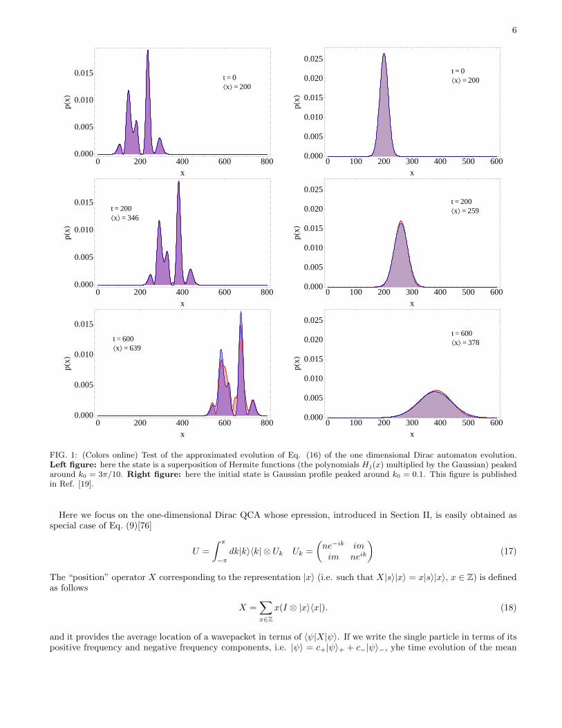
FIG. 2: Zitterbewegung in the one dimensiona Dirac QCA. Top: The mass of the particle is m = 0.15. The amplitudes of thesuperposition between positive and negative frequency states are c+ = 1/

√2 c− = i/

√2 respectively. The wavepacket is peaked

around k0 = 0. The shift and oscillation frequency are respectively 〈ψ|X(0) + ZX(0)|ψ〉 = 3.2 and ω(0)/π = 0.05. Middle:m = 0.15, c+ = 1/

√2, c− = 1/

√2, k0 = 0, σ = 40−1. The shift and oscillation frequency are 0 and 0.13, respectively. Bottom:

m = 0.13, c+ =√

2/3, c− = 1/√

3, k0 = 10−2π, σ = 40−1. In this case the particle and antiparticle contribution are notbalanced and the average position drift velocity is thus 〈ψ+|V |ψ+〉+ 〈ψ−|V |ψ−〉 = (|c+|2 − |c−|2)v(k0) = 0.08, correspondingto an average position x+ψ (800) + x−ψ (800) = 464. Notice that for t → ∞ the term 2<[〈ψ+|ZX(t)|ψ−〉, which is responsible of

the oscillation, goes to 0. This figure is published in Ref. [38].

value of the position operator 〈ψ|X(t)|ψ〉 is given by

xψ(t) := 〈ψ|X(t)|ψ〉 = x+ψ (t) + x−ψ (t) + xintψ (t)

x±ψ (t) := 〈ψ±|X(0) + V t|ψ±〉xintψ (t) := 2<[〈ψ+|X(0)− ZX(0) + ZX(t)|ψ−〉] (19)

where V is a time independent operator corresponding to the group velocity and ZX(t) is the operator that givesthe oscillatory motion (see Ref. [38] for the details). We notice that the interference between positive and negativefrequency is responsible of the oscillating term xintψ (t) whose magnitude is bounded by 1/m which in the usual

dimensional units corresponds to the Compton wavelength ~/mc. These results show that xintψ (t) is the automaton

analogue of the Zitterbewegung for a Dirac particle. for t → ∞ the term 2<[〈ψ+|ZX(t)|ψ−〉], which is responsibleof the oscillation, goes to 0 as 1/

√t and only the additional shift contribution given by 2<[〈ψ+|X(0) − ZX(0)|ψ−〉]

survives. In Fig. 2 one can se the simulation of the evolution of states with particle and antiparticle componentssmoothly peaked around some k0.

B. Scattering against a potential barrier

In this section we study the dynamics of the one dimensional Dirac automaton in the presence of a potential. Inthe position representation the one particle evolution of the one dimensioanal Dirac QCA reads as follows:

U :=∑x

(n|x− 1〉〈x| −im|x〉〈x|−im|x〉〈x| n|x+ 1〉〈x|

). (20)

The presence of a potential φ(x), modifies the unitary evolution of Eq. (20) with a position dependent phase as follows(see also Ref [48, 49]):

Uφ :=∑x

e−iφ(x)(n|x− 1〉〈x| −im|x〉〈x|−im|x〉〈x| n|x+ 1〉〈x|

).

We now review the analysis (carried on in Ref. [38]) of the case in which φ(x) := φ θ(x) (θ(x) is the Heaviside stepfunction) that is a potential step which is 0 for x < 0 and has a constant value φ ∈ [0, 2π] for x ≥ 0. Let us considerthe situation in which, for t� 0, the state is a positive frequency wavepacket peaked around k0 that moves at groupvelocity v(k0) and hits the barrier form the left. Then and one can show that for t � 0 the state is evolved into asuperposition of a reflected and a transmitted wavepacket as follows (we use the notation of Eq. (14) adapted at the

8

0.0 0.5 1.0 1.5 2.0 2.5 3.00.0

0.2

0.4

0.6

0.8

1.0

Φ

R

0.0 0.5 1.0 1.5 2.0 2.5 3.00.0

0.2

0.4

0.6

0.8

1.0

Φ

vHk'

0L

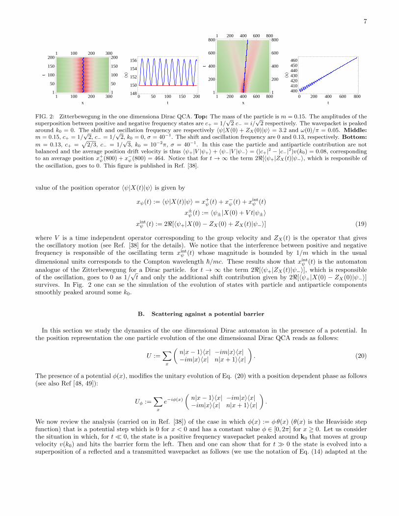
FIG. 3: Reflection coefficient for m = 0.4 and wave-vector of the incident particle k0 = 2 as a function of the potential barrierheight φ. This Figure is published in Ref. [38].

one-dimensional case):

|ψ(t)〉 t�0−−−→ β(k0)

∫dk√2π

gk0(k)e−iω(k)t|u〉−k|k〉+

+ γ(k0)e−iφt∫

dk√2π

gk′0(k′)e−iω(k′)t|u〉k′ |k′〉

where we defined

k′0 s.t. ω(k′0) = ω(k0)− φ,

γ(k0) := γ(k0)

√v(k′0)

v(k0), gk′0(k′) =

√v(k′0)

v(k0)gk′0(k′)

(one can check∫

dk√2π|gk′0(k′)|2 = 1), whose group velocities are −v(k0) for the reflected wave packet and v(k′0) for the

transmitted wave packet.The probability of finding the particle in the reflected wavepacket is then R = |β(k0)|2 (reflection coefficient) while

the probability of finding the particle in the transmitted wavepacket is T = |γ(k0)|2 (trasmission coefficient). Theconsistency of the result can be verified by checking that R + T = 1. Clearly φ = 0 implies R = 0 and increasing φfor a fixed k increases the value of R up to R = 1. By further increasing φ a transmitted wave reappears and thereflection coefficient decreases. This is the so called “Klein paradox” which is originated by the presence of positiveand negative frequency eigenvalues of the unitary evolution. The width of the R = 1 region is an increasing functionof the mass equal to 2 arccos(n) which is the gap between positive and negative frequency solutions.

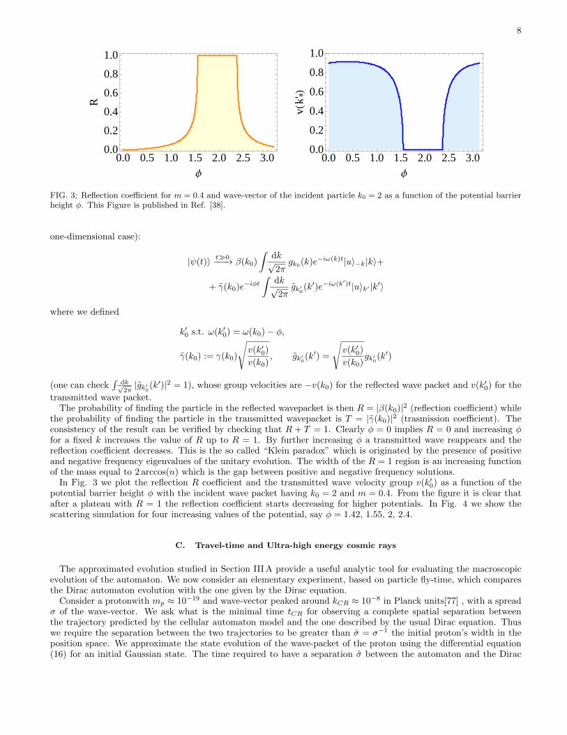
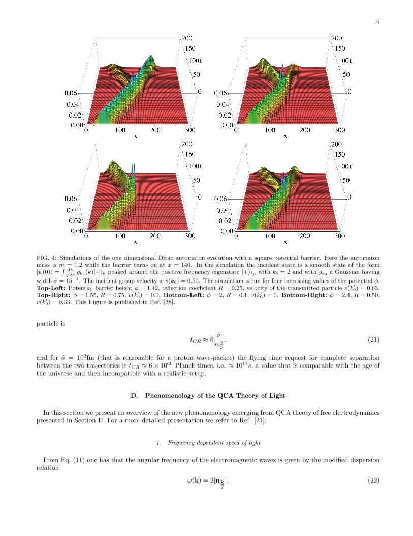
In Fig. 3 we plot the reflection R coefficient and the transmitted wave velocity group v(k′0) as a function of thepotential barrier height φ with the incident wave packet having k0 = 2 and m = 0.4. From the figure it is clear thatafter a plateau with R = 1 the reflection coefficient starts decreasing for higher potentials. In Fig. 4 we show thescattering simulation for four increasing values of the potential, say φ = 1.42, 1.55, 2, 2.4.

C. Travel-time and Ultra-high energy cosmic rays

The approximated evolution studied in Section III A provide a useful analytic tool for evaluating the macroscopicevolution of the automaton. We now consider an elementary experiment, based on particle fly-time, which comparesthe Dirac automaton evolution with the one given by the Dirac equation.

Consider a protonwith mp ≈ 10−19 and wave-vector peaked around kCR ≈ 10−8 in Planck units[77] , with a spreadσ of the wave-vector. We ask what is the minimal time tCR for observing a complete spatial separation betweenthe trajectory predicted by the cellular automaton model and the one described by the usual Dirac equation. Thuswe require the separation between the two trajectories to be greater than σ = σ−1 the initial proton’s width in theposition space. We approximate the state evolution of the wave-packet of the proton using the differential equation(16) for an initial Gaussian state. The time required to have a separation σ between the automaton and the Dirac

9

FIG. 4: Simulations of the one dimensional Dirac automaton evolution with a square potential barrier. Here the automatonmass is m = 0.2 while the barrier turns on at x = 140. In the simulation the incident state is a smooth state of the form|ψ(0)〉 =

∫dk√2πgk0(k)|+〉k peaked around the positive frequency eigenstate |+〉k0 with k0 = 2 and with gk0 a Gaussian having

width σ = 15−1. The incident group velocity is v(k0) = 0.90. The simulation is run for four increasing values of the potential φ.Top-Left: Potential barrier height φ = 1.42, reflection coefficient R = 0.25, velocity of the transmitted particle v(k′0) = 0.63.Top-Right: φ = 1.55, R = 0.75, v(k′0) = 0.1. Bottom-Left: φ = 2, R = 0.1, v(k′0) = 0. Bottom-Right: φ = 2.4, R = 0.50,v(k′0) = 0.33. This Figure is published in Ref. [38].

particle is

tCR ≈ 6σ

m2p

. (21)

and for σ = 102fm (that is reasonable for a proton wave-packet) the flying time request for complete separationbetween the two trajectories is tCR ≈ 6× 1060 Planck times, i.e. ≈ 1017s, a value that is comparable with the age ofthe universe and then incompatible with a realistic setup.

D. Phenomenology of the QCA Theory of Light

In this section we present an overview of the new phenomenology emerging from QCA theory of free electrodynamicspresented in Section II. For a more detailed presentation we refer to Ref. [21].

1. Frequency dependent speed of light

From Eq. (11) one has that the angular frequency of the electromagnetic waves is given by the modified dispersionrelation

ω(k) = 2|nk2

|. (22)

10

and the usual relation ω(k) = |k| is recovered in only the |k| � 1 regime. The speed of light is the group velocity ofthe electromagnetic waves, i.e. the gradient of the dispersion relation. The major consequence of Eq. (22) is that thespeed of light depends on the value of k, as if the vacuum were a dispersive medium.

The phenomenon of a k-dependent speed of light is also studied in the quantum gravity literature where manyauthors considered the hypothesis that the existence of an invariant length (the Planck scale) could manifest itselfin terms of dispersion relations that differ from the usual relativistic one [28–32]. In these models the k-dependentspeed of light c(k), at the leading order in k := |k|, is expanded as c(k) ≈ 1 ± ξkα, where ξ is a numerical factor oforder 1, while α is an integer. This is exactly what happens in our framework, where the intrinsic discreteness of thequantum cellular automata leads to the dispersion relation of Eq. (22) from which the following k-dependent speedof light

c(k) ≈ 1± 3kxkykz|k|2 ≈ 1± 1√

3k, (23)

can be obtained by computing the modulus of the group velocity and power expanding in k with the assumptionkx = ky = kz = 1√

3k, k = |k|. The ± sign in Eq. (23) depends on whether we considered the A+(k) or the A−(k) Weyl

QCA. This prediction can possibly be experimentally tested in the astrophysical domain, where tiny corrections aremagnified by the huge time of flight. For example, observations of the arrival times of pulses originated at cosmologicaldistances, like in some γ-ray bursts[50–53], are now approaching a sufficient sensitivity to detect corrections to therelativistic dispersion relation of the same order as in Eq. (23).

kx

ky

kz

k

r!(k)

2nk2 k

E

B

2n k2

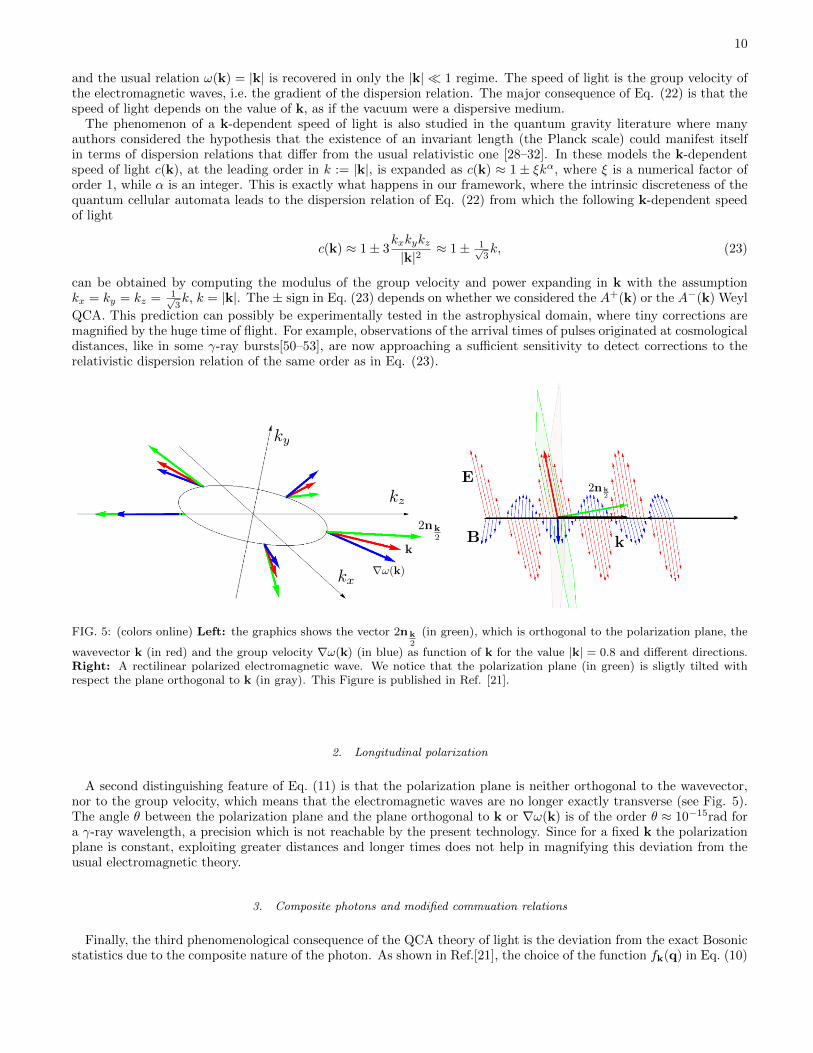
FIG. 5: (colors online) Left: the graphics shows the vector 2nk2

(in green), which is orthogonal to the polarization plane, the

wavevector k (in red) and the group velocity ∇ω(k) (in blue) as function of k for the value |k| = 0.8 and different directions.Right: A rectilinear polarized electromagnetic wave. We notice that the polarization plane (in green) is sligtly tilted withrespect the plane orthogonal to k (in gray). This Figure is published in Ref. [21].

2. Longitudinal polarization

A second distinguishing feature of Eq. (11) is that the polarization plane is neither orthogonal to the wavevector,nor to the group velocity, which means that the electromagnetic waves are no longer exactly transverse (see Fig. 5).The angle θ between the polarization plane and the plane orthogonal to k or ∇ω(k) is of the order θ ≈ 10−15rad fora γ-ray wavelength, a precision which is not reachable by the present technology. Since for a fixed k the polarizationplane is constant, exploiting greater distances and longer times does not help in magnifying this deviation from theusual electromagnetic theory.

3. Composite photons and modified commuation relations

Finally, the third phenomenological consequence of the QCA theory of light is the deviation from the exact Bosonicstatistics due to the composite nature of the photon. As shown in Ref.[21], the choice of the function fk(q) in Eq. (10)

11

determines the regime where the composite photon can be approximately treated as a Boson. However, independentlyon the details of function fk(q), one can prove that a Fermionic saturation of the Boson is not visible, e.g. for themost powerful laser [54] one has a approximately an Avogadro number of photons in 10−15cm3, whereas in the samevolume on has around 1090 Fermionic modes. Another test for the composite nature of photons is provided by theprediction of deviations from the Planck’s distribution in Blackbody radiation experiments. A similar analysis wascarried out in Ref. [37], where the author showed that the predicted deviation from Planck’s law is less than one partover 10−8, well beyond the sensitivity of present day experiments.

V. FUTURE PERSPECTIVES

We conclude this paper with an overview of the future developments of the research program on QCA for FieldTheory.

A. Lorentz covariance and Deformed Relativity

Because of the intrinsic discreteness of the model, a dynamical evolution described in terms of a QCA cannot satisfythe usual Lorentz covariance, which must break down at the Planck scale. Moreover the very notions of spacetime andboosted reference frame break down at small scales, and need a thoughtful reconsideration. In Ref. [55] a definitionof reference frame was introduced in a background-free scenario, in terms of labelling of irreducible representationsof the group G. The Lorentz symmetry is then recovered by imposing a generalized relativity principle on possiblechanges of reference frame, allowing only those changes that leave the automaton invariant. A preliminary analysisof the one-dimensional case can be found in Ref. [56], where only the necessary condition of preserving the dispersionrelation was considered. Focusing on the one dimensional Dirac QCA we have

ω(k) = arccos(√

1−m2 cos(k)) (24)

and one can see that in the k � 1,m � 1 limit Eq. (24) reduces to the usual relativistic dispersion relation ω2 =k2 + m2. It is also immediate to check that the automaton dispersion relation of Eq. (24) is not invariant understandard Lorentz transformation. In order to preserve Eq. (24) one needs to introduce a non-linear representation ofthe Lorentz transformation in the wave-vector space—as proposed in the so called deformed special relativity (DSR)models [31, 32, 57–60].

In Ref. [55] the boosts preserving the three-dimensional Weyl automaton were then derived in the form of thefollowing non-linear representation of the Lorentz group

LDβ := D−1 ◦ Lβ ◦ D, (25)

where D : R4 → R4 is a non-linear map. The specific form of D gives rise to a particular frequency/wave-vectorLorentz deformation.

These ideas can also be applied to the three-dimensional Dirac QCA. In this case one can show that a change ofthe rest mass should be involved in the representation of boosts, in order to obey our generalized relativity principle.Interestingly, this unexpected feature gives rise to an emergent space-time with a non-linear de Sitter symmetryinstead of the Lorentz one.

Another challenging line of research is to characterize the emergent spacetime of the QCA framework. The DSRmodels provide a complete description of Lorentz symmetry in frequency/wave-vector space but there are heuristicways to extend this framework to the position-time space. Relative locality [61, 62], non-commutative spacetime [63]and Hopf algebra symmetries [64, 65] have been considered in order to give a real space formulation of deformedrelativity.

Finally, we would like to stress that space-time emerges from: i) the structure of the group G, ii) the specificexpression of the automaton and iii) the generalized relativity principle, while all these concepts do not require anyspace-time background. Thus, outside the limits in which the relativistic approximations hold, the very structure ofour usual space-time break down, substituted by other counterintuitive effects. In particular this is true in all physicalsituations where the discrete structure of the lattice G becomes relevant.

B. Thermodynamics of free ultra-relativistic particles and QCA

Most of the analysis that we presented in this paper was focused on the dynamics of one particle state and thedeviations of this kinematics from the usual relativistic one. On the other hand, it would be interesting to explore the

12

QCA phenomenology when the number of particle goes to infinity, namely a thermodynamic limit. Since the QCAwe are considering descrive a non-interacting dynamics, the thermodynamic that will emerge will describe a gas offree particles. However, since the dispersion relation of the QCA differs from the relativistic one, the density of stateswill be different.

In the case of free fermions this will result in a shift of the Fermi energy that could become relevant when thenumber of fermions becomes very large. One could for example analyze how the Chandrasekhar limit of white dwarfsis modified in this context (see Ref. [66, 67] for a similar analysis in a different context).

C. Interacting extensions

The theory of linear QCAs naturally leads to free quantum field theories. In order to introduce interactions, oneneeds to relax the linearity assumption. This can be done by splitting the computational step in two stages, thefirst one acting linearly, and the second one representing a nonlinear and completely local evolution. This can bemotivated in terms of a time-local gauge symmetry that must preserve some local degree of freedom, in particular thelocal number of excitations. This simple modification of the linear automaton introduces a non-trivial interaction,making the automaton non-trivially reducible to a quantum walk. Preliminary analysis shows that this minimalrelaxation of linearity is sufficient to give rise to couplings that might reproduce the phenomenology of quantumelectrodynamics.

Acknowledgements

This work has been supported in part by the Templeton Foundation under the project ID# 43796 A Quantum-Digital Universe.

[1] A. Bisio, G. M. D’Ariano, P. Perinotti, and A. Tosini, Foundations of Physics 45, 1137 (2015).[2] J. von Neumann, Theory of self-reproducing automata (University of Illinois Press, Urbana and London, 1966).[3] G. Hooft, arXiv preprint arXiv:1405.1548 (2014).[4] H.-T. Elze, Physical Review A 89, 012111 (2014).[5] R. Feynman, International journal of theoretical physics 21, 467 (1982).[6] B. Schumacher and R. Werner, Arxiv preprint quant-ph/0405174 (2004).[7] P. Arrighi, V. Nesme, and R. Werner, Journal of Computer and System Sciences 77, 372 (2011).[8] D. Gross, V. Nesme, H. Vogts, and R. Werner, Communications in Mathematical Physics , 1 (2012).[9] G. Grossing and A. Zeilinger, Complex Systems 2, 197 (1988).

[10] Y. Aharonov, L. Davidovich, and N. Zagury, Physical Review A 48, 1687 (1993).[11] A. Ambainis, E. Bach, A. Nayak, A. Vishwanath, and J. Watrous, in Proceedings of the thirty-third annual ACM symposium

on Theory of computing (ACM, 2001) pp. 37–49.[12] D. Reitzner, D. Nagaj, and V. Buzek, Acta Physica Slovaca. Reviews and Tutorials 61, 603 (2011).[13] A. M. Childs, R. Cleve, E. Deotto, E. Farhi, S. Gutmann, and D. A. Spielman, in Proceedings of the thirty-fifth annual

ACM symposium on Theory of computing (ACM, 2003) pp. 59–68.[14] A. Ambainis, SIAM Journal on Computing 37, 210 (2007).[15] F. Magniez, M. Santha, and M. Szegedy, SIAM Journal on Computing 37, 413 (2007).[16] E. Farhi, J. Goldstone, and S. Gutmann, arXiv preprint quant-ph/0702144 (2007).[17] G. D’Ariano, CP1232 Quantum Theory: Reconsideration of Foundations 5 (arXiv:1001.1088) 3 (2010).[18] G. M. D’Ariano, Phys. Lett. A 376 (2011).[19] A. Bisio, G. M. D’Ariano, and A. Tosini, Annals of Physics 354, 244 (2015).[20] G. M. D’Ariano and P. Perinotti, Phys. Rev. A 90, 062106 (2014).[21] A. Bisio, G. M. D’Ariano, and P. Perinotti, arXiv preprint arXiv:1407.6928 (2014).[22] P. Arrighi, V. Nesme, and M. Forets, Journal of Physics A: Mathematical and Theoretical 47, 465302 (2014).[23] P. Arrighi and S. Facchini, EPL (Europhysics Letters) 104, 60004 (2013).[24] T. C. Farrelly and A. J. Short, Physical Review A 89, 012302 (2014).[25] T. C. Farrelly and A. J. Short, arXiv preprint arXiv:1312.2852 (2013).[26] G. M. D’Ariano, N. Mosco, P. Perinotti, and A. Tosini, Physics Letters A 378, 3165 (2014).[27] G. D’Ariano, N. Mosco, P. Perinotti, and A. Tosini, arXiv preprint arXiv:1410.6032 (2014).[28] J. Ellis, N. Mavromatos, and D. V. Nanopoulos, Physics Letters B 293, 37 (1992).[29] J. Lukierski, H. Ruegg, and W. J. Zakrzewski, Annals of Physics 243, 90 (1995).[30] G. ’t Hooft, Class. Quantum Grav. 13, 1023 (1996).

13

[31] G. Amelino-Camelia, Physics Letters B 510, 255 (2001).[32] J. Magueijo and L. Smolin, Phys. Rev. Lett. 88, 190403 (2002).[33] L. De Broglie, Une nouvelle conception de la lumiere, Vol. 181 (Hermamm & Cie, 1934).[34] P. Jordan, Zeitschrift fur Physik 93, 464 (1935).[35] R. d. L. Kronig, Physica 3, 1120 (1936).[36] W. Perkins, Physical Review D 5, 1375 (1972).[37] W. Perkins, International Journal of Theoretical Physics 41, 823 (2002).[38] A. Bisio, G. M. D’Ariano, and A. Tosini, Phys. Rev. A 88, 032301 (2013).[39] S. Succi and R. Benzi, Physica D: Nonlinear Phenomena 69, 327 (1993).[40] I. Bialynicki-Birula, Physical Review D 49, 6920 (1994).[41] D. Meyer, Journal of Statistical Physics 85, 551 (1996).

[42] E. Schrodinger, Uber die kraftefreie Bewegung in der relativistischen Quantenmechanik (Akademie der wissenschaften inkommission bei W. de Gruyter u. Company, 1930).

[43] D. Lurie and S. Cremer, Physica 50, 224 (1970).[44] F. Cannata and L. Ferrari, Physical Review B 44, 8599 (1991).[45] L. Ferrari and G. Russo, Physical Review B 42, 7454 (1990).[46] F. Cannata, L. Ferrari, and G. Russo, Solid State Communications 74, 309 (1990).[47] X. Zhang, Phys. Rev. Lett. 100, 113903 (2008).[48] P. Kurzynski, Physics Letters A 372, 6125 (2008).[49] D. A. Meyer, International Journal of Modern Physics C 8, 717 (1997).[50] G. Amelino-Camelia, J. Ellis, N. Mavromatos, D. V. Nanopoulos, and S. Sarkar, Nature 393, 763 (1998).[51] A. Abdo, M. Ackermann, M. Ajello, K. Asano, W. Atwood, M. Axelsson, L. Baldini, J. Ballet, G. Barbiellini, M. Baring,

et al., Nature 462, 331 (2009).[52] V. Vasileiou, A. Jacholkowska, F. Piron, J. Bolmont, C. Couturier, J. Granot, F. Stecker, J. Cohen-Tanugi, and F. Longo,

Physical Review D 87, 122001 (2013).[53] G. Amelino-Camelia and L. Smolin, Physical Review D 80, 084017 (2009).[54] M. Dunne, in Conference on Lasers and Electro-Optics/Pacific Rim (Optical Society of America, 2007) pp. 1–2.[55] A. Bisio, G. M. D’Ariano, and P. Perinotti, arXiv preprint arXiv:1503.01017 (2015).[56] A. Bibeau-Delisle, A. Bisio, G. M. D’Ariano, P. Perinotti, and A. Tosini, arXiv preprint arXiv:1310.6760 (2013).[57] G. Amelino-Camelia, International Journal of Modern Physics D 11, 35 (2002).[58] G. Amelino-Camelia and T. Piran, Physical Review D 64, 036005 (2001).[59] G. Amelino-Camelia, Modern Physics Letters A 17, 899 (2002).[60] J. Magueijo and L. Smolin, Physical Review D 67, 044017 (2003).[61] G. Amelino-Camelia, L. Freidel, J. Kowalski-Glikman, and L. Smolin, International Journal of Modern Physics D 20,

2867 (2011).[62] G. Amelino-Camelia, V. Astuti, and G. Rosati, The European Physical Journal C 73, 1 (2013).[63] A. Connes and J. Lott, Nuclear Physics B-Proceedings Supplements 18, 29 (1991).[64] J. Lukierski, H. Ruegg, A. Nowicki, and V. N. Tolstoy, Physics Letters B 264, 331 (1991).[65] S. Majid and H. Ruegg, Physics Letters B 334, 348 (1994).[66] G. Amelino-Camelia, N. Loret, G. Mandanici, and F. Mercati, International Journal of Modern Physics D 21 (2012).[67] A. Camacho, Classical and Quantum Gravity 23, 7355 (2006).[68] S. Albeverio, R. Cianci, and A. Y. Khrennikov, P-Adic Numbers, Ultrametric Analysis, and Applications 1, 91 (2009).[69] M. Takeda, N. Hayashida, K. Honda, N. Inoue, K. Kadota, F. Kakimoto, K. Kamata, S. Kawaguchi, Y. Kawasaki,

N. Kawasumi, et al., Physical Review Letters 81, 1163 (1998).[70] Other approaches to discrete space-time based on p-adic numbers were studied in Refs. [68].[71] We denote as [A,B]+ the anticommutator AB +BA. The commutator AB −BA will be denoted as [A,B]−.[72] This step would requires a more precise mathematical characterization (which we omit) of the presented assumptions. See

Ref. [20] for the details.[73] In order to prove this step one need a stronger isotropy condition than the one presented in the text. See Ref. [20] for the

details.[74] We denote as A∗ the complex conjugate of A[75] Since a QCA describe an evolution which discrete in time, the derivative with respect time is not defined in this context.

However we can imagine Atk to be defined for any real value of t and then derive with respect the continuous variable t.This is the construction which underlies Eq. (11)

[76] More precisely, Eq. (8) leads to two identical copies of Eq. (17)[77] As for order of magnitude, we consider numerical values corresponding to ultra high energy cosmic rays (UHECR) [69]