Autofluorescence imaging of NADH and flavoproteins in the rat brain: insights from Monte Carlo simulations

Autofluorescence imaging of NADH and flavoproteins in the rat brain: insights from

Monte Carlo simulations.

Barbara L’Heureux,1,* Hirac Gurden,1

and Frédéric Pain1

1UMR8165 “Imagerie et Modélisation en Neurobiologie et Cancérologie”, CNRS/Université Paris XI/Paris VII,

Bat 440, Campus d’Orsay, 91406 Orsay, France *Corresponding author: [email protected]

Abstract: There has been recently a renewed interest in using

Autofluorescence imaging (AF) of NADH and flavoproteins (Fp) to

map brain activity in cortical areas. The recording of these cellular

signals provides complementary information to intrinsic optical imaging

based on hemodynamic changes. However, which of NADH or Fp is

the best candidate for AF functional imaging is not established, and the

temporal profile of AF signals is not fully understood. To bring new

theoretical insights into these questions, Monte Carlo simulations of AF

signals were carried out in realistic models of the rat somatosensory

cortex and olfactory bulb. We show that AF signals depend on the

structural and physiological features of the brain area considered and

are sensitive to changes in blood flow and volume induced by sensory

activation. In addition, we demonstrate the feasibility of both NADH-

AF and Fp-AF in the olfactory bulb.

2009 Optical Society of America

OCIS codes: (170.3880) Medical and biological imaging; (170.3660 ) Light propagation

in tissues; (180.2520) Fluorescence microscopy

References and links

1. T. Bonhoeffer and Grinvald A, “Optical Imaging based on intrinsic signals: the methodology” in

Brain mapping; the methods”. A.W. Toga and J.C. Mazziotta, Eds. (Academic Press, Los Angeles,

CA, 1996).

2. B. Chance, P. Cohen, F. Jöbsis, B. Schoener, “Intracellular oxidation-reduction states in vivo,”

Science 137, 499-508 (1962).

3. B. Chance, “The kinetics of flavoprotein and pyridine nucleotide oxidation in cardiac mitochondria in

the presence of calcium,” FEBS Lett. 26, 315-9 (1972).

4. M. Hashimoto, Y. Takeda, T. Sato, H. Kawahara, O. Nagano and M. Hirakawa, “Dynamic changes of

NADH fluorescence images and NADH content during spreading depression in the cerebral cortex of

gerbils,” Brain. Res. 872, 294-300 (2000).

5. R.E. Anderson and F.B. Meyer, “In vivo fluorescent imaging of NADH redox state in brain,” Methods

Enzymol. 352, 482-94 (2002).

6. A. Mayevsky and G.G. Rogatsky, “Mitochondrial function in vivo evaluated by NADH fluorescence:

from animal models to human studies,” Am. J. Physiol. Cell. Physiol. 292, C615-40 (2007).

7. K.C. Reinert, R.L. Dunbar, W. Gao, G. Chen, T.J. Ebner, “Flavoprotein autofluorescence imaging of

neuronal activation in the cerebellar cortex in vivo,” J. Neurophysiol. 92,199-211 (2004).

8. K. Shibuki, R. Hishida, H. Murakami, M. Kudoh, T. Kawaguchi, M. Watanabe, S. Watanabe, T.

Kouuchi, R. Tanaka., “Dynamic imaging of somatosensory cortical activity in the rat visualized by

flavoprotein autofluorescence,” J. Physiol. 549, 919-27 (2003).

9. H. Murakami, D. Kamatani, R. Hishida, T. Takao, M. Kudoh, T. Kawaguchi, R. Tanaka, K.Shibuki,

“Short-term plasticity visualized with flavoprotein autofluorescence in the somatosensory cortex of

anaesthetized rats,” Eur. J. Neurosci. 19, 1352-60 (2004).

10. M. Tohmi, H. Kitaura, S. Komagata, M. Kudoh, K. Shibuki, “Enduring critical period plasticity

visualized by transcranial flavoprotein imaging in mouse primary visual cortex,” J. Neurosci. 26,

11775-85 (2006).

11. Y. Kubota, D. Kamatani, H. Tsukano, S. Ohshima, K. Takahashi, R. Hishida, M. Kudoh, S.

Takahashi, K. Shibuki, “Transcranial photo-inactivation of neural activities in the mouse auditory

cortex,” Neurosci. Res. 60, 422-30 (2008).

12. K.C. Reinert, W. Gao, G. Chen, T.J. Ebner, “Flavoprotein autofluorescence imaging in the cerebellar

#104037 - $15.00 USD Received 17 Nov 2008; revised 30 Jan 2009; accepted 9 Mar 2009; published 22 May 2009

(C) 2009 OSA 8 June 2009 / Vol. 17, No. 12 / OPTICS EXPRESS 9477

cortex in vivo,” J. Neurosci. Res. 85, 3221-32 (2007).

13. B. Weber, C. Burger, M.T. Wyss, G.K. von Schulthess, F. Scheffold, A. Buck, “Optical imaging of

the spatiotemporal dynamics of cerebral blood flow and oxidative metabolism in the rat barrel cortex,”

Eur. J. Neurosci. 20, 2664-70 (2004).

14. H. Gurden, N. Uchida, et Z.F. Mainen, “Sensory-evoked intrinsic optical signals in the olfactory bulb

are coupled to glutamate release and uptake,” Neuron 52, 335-45 (2006).

15. G.C. Petzold, D.F. Albeanu, T.F. Sato, V.N. Murthy, “Coupling of neural activity to blood flow in

olfactory glomeruli is mediated by astrocytic pathways,” Neuron 58, 897-910 (2008).

16. C.W. Shuttleworth, A.M. Brennan, et J.A. Connor, “NAD(P)H fluorescence imaging of postsynaptic

neuronal activation in murine hippocampal slices,” J Neurosci. 23, 3196-208 (2003).

17. S. A. Prahl, “Optical Absorption of Hemoglobin,” http://omlc.ogi.edu/spectra/hemoglobin/index.html

18. C.C.H. Petersen, “The barrel cortex--integrating molecular, cellular and systems physiology,” Pflugers

Arch. 447, 126-34 (2003).

19. T.A. Woolsey, C.M. Rovainen, S.B. Cox, M.H. Henegar, G.E. Liang, D. Liu, Y.E. Moskalenko, J. Sui,

L. Wei, “Neuronal units linked to microvascular modules in cerebral cortex: response elements for

imaging the brain,” Cereb. Cortex. 6, 647-60 (1991).

20. G.M. Shepherd, “Synaptic organization of the mammalian olfactory bulb,” Physiol. Rev. 52, 864-917

(1972).

21. E. Chaigneau, M. Oheim, E. Audinat, S. Charpak, “Two-photon imaging of capillary blood flow in

olfactory bulb glomeruli,” Proc. Natl. Acad. Sci. U. S. A. 100, 13081-6 (2003).

22. M. Kohl, U. Lindauer, G. Royl, M. Kuhl, L. Gold, A. Villringer, U. Dirnagl., “Physical model for the

spectroscopic analysis of cortical intrinsic optical signals,” Phys. Med. Biol. 45, 3749-64 (2000).

23. N. Plesnila, C. Putz, M. Rinecker, J. Wiezorrek, L. Schleinkofer, A.E. Goetz, W.M. Kuebler,

“Measurement of absolute values of hemoglobin oxygenation in the brain of small rodents by near

infrared reflection spectrophotometry,” J. Neurosci. Methods 114, 107-17 (2002).

24. J.C. Nawroth, C.A. Greer, W.R. Chen, S.B. Laughlin, G.M. Shepherd, “An energy budget for the

olfactory glomerulus,” J. Neurosci. 27, 9790-800 (2007).

25. A.N. Yaroslavsky, P.C. Schulze, I.V. Yaroslavsky, R. Schober, F. Ulrich, H.J. Schwarzmaier, “Optical

properties of selected native and coagulated human brain tissues in vitro in the visible and near

infrared spectral range,” Phys. Med. Biol. 47, 2059-73 (2002).

26. E.M. Hillman, A. Devor, M.B. Bouchard, A.K. Dunn, G.W. Krauss, J. Skoch, B.J. Bacskai, A.M.

Dale, D.A. Boas, “Depth-resolved optical imaging and microscopy of vascular compartment dynamics

during somatosensory stimulation,” Neuroimage 35, 89-104 (2007).

27. M. Jones, J. Berwick, et J. Mayhew, “Changes in blood flow, oxygenation, and volume following

extended stimulation of rodent barrel cortex,” Neuroimage 15, 474-87 (2002).

28. J. Mayhew, Y. Zheng, Y. Hou, B. Vuksanovic, J. Berwick, S. Askew, P. Coffey, “Spectroscopic

analysis of changes in remitted illumination: the response to increased neural activity in brain,”

Neuroimage 10, 304-26 (1999).

29. A. Devor, A. K. Dunn, M. L. Andermann, I. Ulbert, D. A. Boas, A. M. Dale1 “Coupling of total

hemoglobin concentration, oxygenation, and neural activity in rat somatosensory cortex,” Neuron 39,

353-9 (2003).

30. S. A. Prahl, M. Keijzer, S. L. Jacques, A. J. Welch, “A Monte Carlo Model of Light Propagation in

Tissue,” Proc. SPIE IS 5, 102-11(1989).

31. L. Wang, S.L. Jacques, et L. Zheng, “MCML-Monte Carlo modeling of light transport in multi-

layered tissues,” Comput. Methods Programs Biomed. 47, 131-46 (1995).

32. F. Agner, “Pseudo random number generator;” http://www.agner.org/random/mother.

33. B. Chance, B. Schoener, R. Oshino, F. Itshak, Y. Nakase, “Oxidation-reduction ratio studies of

mitochondria in freeze-trapped samples. NADH and flavoprotein fluorescence signals,” J. Biol. Chem.

254, 4764-71 (1979).

34. R.C. Benson, R.A. Meyer, M.E. Zaruba, G.M. McKhann, “Cellular autofluorescence--is it due to

flavins?,” J. Histochem. Cytochem. 27, 44-8 (1979).

35. A.M. Brennan, J.A. Connor, et C.W. Shuttleworth, “Modulation of the amplitude of NAD(P)H

fluorescence transients after synaptic stimulation,” J. Neurosci. Res. 85, 3233-43 (2007).

36. A.M. Brennan, J.A. Connor, et C.W. Shuttleworth, “NAD(P)H fluorescence transients after synaptic

activity in brain slices: predominant role of mitochondrial function,” J. Cereb. Blood Flow. Metab. 26,

1389-406 (2006).

37. T.R. Husson, A.K. Mallik, J.X. Zhang, N.P. Issa, “Functional imaging of primary visual cortex using

flavoprotein autofluorescence,” J. Neurosci. 27, 8665-75 (2007).

38. R. Scholz, R.G. Thurman, J.R. Williamson, B. Chance, T. Bücher., “Flavin and pyridine nucleotide

oxidation-reduction changes in perfused rat liver. I. Anoxia and subcellular localization of fluorescent

flavoproteins,” J. Biol. Chem. 244, 2317-24 (1969).

39. F.F. Jöbsis, M. O'Connor, A. Vitale, H. Vreman, “Intracellular redox changes in functioning cerebral

cortex. I. Metabolic effects of epileptiform activity,” J. Neurophysiol. 34, 735-49 (1971).

40. F. Xu, I. Kida, F. Hyder, R.G. Shulman, “Assessment and discrimination of odor stimuli in rat

olfactory bulb by dynamic functional MRI,” Proc Natl Acad Sci U S A. 97, 10601-6. (2000).

41. B.A. Johnson, M. Leon, “Spatial distribution of [14C]2-deoxyglucose uptake in the glomerular layer

of the rat olfactory bulb following early odor reference learning,” J Comp Neurol. 37, 6557-66. (1996)



http://omlc.ogi.edu/spectra/hemoglobin/index.html

42. O. Wolfbeis, “Fluorescence of organic natural products,” in Molecular Luminescence Spectroscopy.

Part 1: Methods and Applications, John Wiley and Sons, ed. (S. G. Schulman, 1985), pp. 167-370.

43. A. Grinvald, E. Lieke, R.D. Frostig, C.D. Gilbert, T.N. Wiesel, “Functional architecture of cortex

revealed by optical imaging of intrinsic signals,” Nature 324, 361-4 (1986).

44. M. Jones, J. Berwick, J. Mayhew, “Changes in blood flow, oxygenation, and volume following

extended stimulation of rodent barrel cortex,” Neuroimage 15, 474-87 (2002).

45. Prakash, J.D. Biag, S.A. Sheth, S. Mitsuyama, J. Theriot, C. Ramachandra, A.W. Toga, “Temporal

profiles and 2-dimensional oxy-, deoxy-, and total-hemoglobin somatosensory maps in rat versus

mouse cortex,” Neuroimage 37 Suppl 1, S27-36 (2007).

1. Introduction

Endogenous optical signals arise from molecular mechanisms linked to neuroenergetics

and are routinely used to map sensory activation of neural networks. These signals can be

divided into two groups according to the vascular or the cellular compartment that they

sample in the brain tissue. Intrinsic Optical signals (IOS) are tightly coupled to changes in

vascular dynamics. They are produced during activation by a local decrease in red light

reflectance due to changes in blood oxygenation level and blood volume [1]. Since the

mid 80’s, IOS imaging has provided with unique insights into the functional architecture

of the visual, auditory, somatosensory and olfactory systems [1]. On the other hand,

cellular fluorescence or autofluorescence (AF) signals monitor the activity of energetic

cycles in vivo because they are related to changes in the redox state of metabolic

intermediates such as Nicotinamide Adenine Dinucleotide (NADH) and flavoproteins

(Fp). NADH-AF has been used for a long time in optical spectroscopy [2] and imaging

[3] experiments. Recent improvements in the sensitivity of scientific imaging CCD

cameras have allowed in vivo imaging of NADH-AF with adequate temporal resolution

[4-6] and the use of Fp-AF for functional brain imaging [7,8]. AF signals imaging has

allowed visualization of activity-dependent changes in many sensory structures [7-13].

However, to our knowledge, AF recordings have not been reported in the olfactory bulb

(OB) despite the great interest of this structure to the study of neurovascular and

neuroenergetics coupling following sensory stimulation [14,15]. In particular, the OB is

constituted of remarkably well-defined functional modules, the olfactory glomeruli, which

are easily accessible for functional optical imaging and can be stimulated by odorants at

controlled physiological intensities and durations.

Although potentially interesting for high resolution imaging, AF signals are not fully

understood because of three incompletely addressed questions. First, which of NADH or

Fp is the best candidate for in vivo AF signals imaging is unclear. Second, the spatial

location in depth and extension of the source of the recorded AF signals within brain

tissues have not been studied so far. Third, the quantification of the putative

contamination of AF signals by activity-dependent hemodynamic changes (leading to

changes in light absorption and scattering) is still lacking for in vivo studies. In this view,

attempts were made to separate the AF signals and hemodynamic responses by

pharmacological studies in brain slices [8,16] or in vivo [8,12]. These studies have shown

that some components of AF signals are clearly not due to vascular effects. However,

quantitation of the vascular contamination to in vivo AF signals is difficult since the

selective inhibition of hemodynamic responses by nitric oxide synthase is only partial as

underlined in reference [8].

To date, no theoretical quantitative approach has been applied to describe optical

changes during brain activation and their influence on sensory-evoked AF signals

recorded in vivo. In the present article, we have carried out Monte Carlo (MC) simulations

to study the physical aspects of AF signals recordings following sensory activation in the

somatosensory cortex (SsC) and OB.

2. Materials and methods

We performed standard MC simulations of optical photons travel through biological

tissues [17] in anatomofunctional models of the SsC and OB. For NADH and Fp, we



considered photons with the following wavelengths: NADH excitation at 350 nm and

emission at 440 nm, and Fp excitation at 440 nm and emission at 530 nm. Since AF

recordings have already been reported in the rat SsC in vivo, we first performed MC

simulations in the SsC and then made a comparison with the OB.

2.1 Geometrical properties of the somatosensory cortex model

In rodents, each whisker is represented in a localized column of the neocortex which is

organized in 4 distinct layers classically numbered from L1 to L4 in the dorsoventral axis

from the surface (see Fig. 1). Mechanical stimulation of a whisker activates a specific

thalamic relay, which terminates in layer 4 of the SsC named the “barrel” because of its

cylindrical shape. After initiation in the barrel, the activation then propagates to layers

L3/L2 of the SsC [18]. On the basis of anatomical data [18,19], we chose an average

thickness of 300 µm for each layer with a diameter of 300 µm for the base of the

cylindrical column. Considering the vascularization of these layers, the density of

capillaries is similar in L2, L3 and L4 and higher than in L1 [19]. On the basis of these

anatomofunctional data, we have built a model of SsC constituted of 2 layers: Layer LII

with a width of 900 µm represents the neocortical column and includes L2, L3 and L4,

and layer LI represents cortical tissues above LII (Fig. 1).

2.2 Geometrical properties of the olfactory bulb

The OB is organized in six different layers: the Olfactory Nerve Layer (ONL), the

Glomerular Layer (GL), the external plexiform layer, mitral cell layer, internal plexiform

layer and granular cell layer [20]. Our OB model is constituted of 3 layers. The first is the

ONL, formed by the unmyelinated axons of olfactory receptor neurons located in the

olfactory epithelium. The ONL innervates the GL, which is constituted of spherical

structures of roughly 100 µm diameter, the olfactory glomeruli. As described by

Chaigneau et al. in their in vivo two-photon microscopy study [21], the upper boundary of

the GL is located on average at 140 µm below the surface. Considering these anatomical

data, we have chosen the GL as the second layer of our model and defined it as a layer of

contiguous 100 µm diameter spheres located between 140 and 240 µm of depth. Finally,

as the remaining layers present similar anatomical and vascularization features, their

optical properties were assumed to be identical and were fused into a single “Underneath

the Glomerular Layer” (UGL). UGL is the third layer of our OB model and represents all

tissues between 240 and 1200 µm of depth.

Fig.1. Multi-layer models for the SsC and OB. Left column: the SsC model is constituted

of Layer I (LI) and Layer II (LII), encompassing respectively layer 1 (L1) and layer 2, 3

and 4 (L2, L3, L4). Right column: the OB model is constituted of the olfactory nerve layer



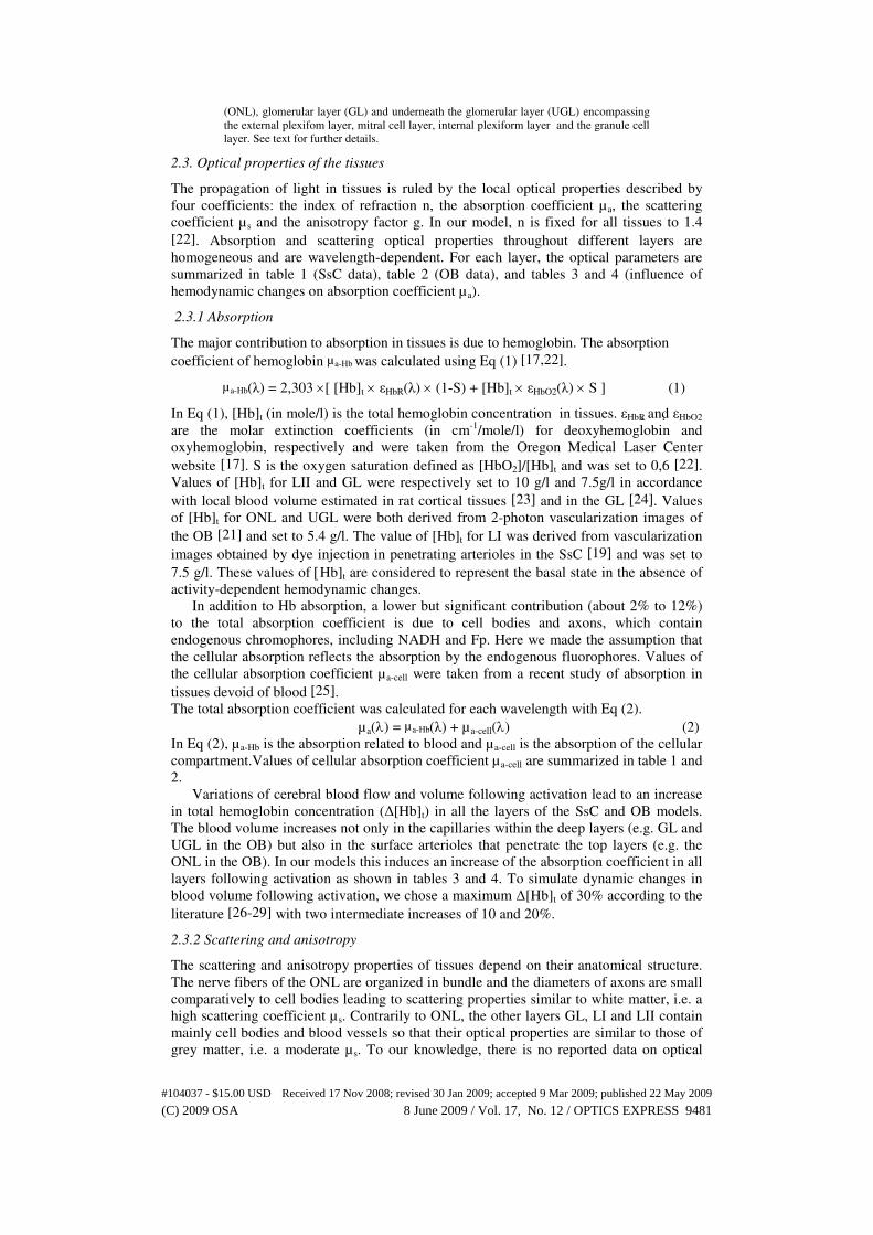
(ONL), glomerular layer (GL) and underneath the glomerular layer (UGL) encompassing

the external plexifom layer, mitral cell layer, internal plexiform layer and the granule cell

layer. See text for further details.

2.3. Optical properties of the tissues

The propagation of light in tissues is ruled by the local optical properties described by

four coefficients: the index of refraction n, the absorption coefficient µa, the scattering

coefficient µ s and the anisotropy factor g. In our model, n is fixed for all tissues to 1.4

[22]. Absorption and scattering optical properties throughout different layers are

homogeneous and are wavelength-dependent. For each layer, the optical parameters are

summarized in table 1 (SsC data), table 2 (OB data), and tables 3 and 4 (influence of

hemodynamic changes on absorption coefficient µa).

2.3.1 Absorption

The major contribution to absorption in tissues is due to hemoglobin. The absorption

coefficient of hemoglobin µa-Hb was calculated using Eq (1) [17,22].

µa-Hb(λ) = 2,303 ×[ [Hb]t × εHbR(λ) × (1-S) + [Hb]t × εHbO2(λ) × S ] (1)

In Eq (1), [Hb]t (in mole/l) is the total hemoglobin concentration in tissues. εHbR and εHbO2

are the molar extinction coefficients (in cm-1/mole/l) for deoxyhemoglobin and

oxyhemoglobin, respectively and were taken from the Oregon Medical Laser Center

website [17]. S is the oxygen saturation defined as [HbO2]/[Hb]t and was set to 0,6 [22].

Values of [Hb]t for LII and GL were respectively set to 10 g/l and 7.5g/l in accordance

with local blood volume estimated in rat cortical tissues [23] and in the GL [24]. Values

of [Hb]t for ONL and UGL were both derived from 2-photon vascularization images of

the OB [21] and set to 5.4 g/l. The value of [Hb]t for LI was derived from vascularization

images obtained by dye injection in penetrating arterioles in the SsC [19] and was set to

7.5 g/l. These values of [Hb]t are considered to represent the basal state in the absence of

activity-dependent hemodynamic changes.

In addition to Hb absorption, a lower but significant contribution (about 2% to 12%)

to the total absorption coefficient is due to cell bodies and axons, which contain

endogenous chromophores, including NADH and Fp. Here we made the assumption that

the cellular absorption reflects the absorption by the endogenous fluorophores. Values of

the cellular absorption coefficient µa-cell were taken from a recent study of absorption in

tissues devoid of blood [25].

The total absorption coefficient was calculated for each wavelength with Eq (2).

µa(λ) = µa-Hb(λ) + µa-cell(λ) (2)

In Eq (2), µa-Hb is the absorption related to blood and µa-cell is the absorption of the cellular

compartment.Values of cellular absorption coefficient µa-cell are summarized in table 1 and

2.

Variations of cerebral blood flow and volume following activation lead to an increase

in total hemoglobin concentration (∆[Hb]t) in all the layers of the SsC and OB models.

The blood volume increases not only in the capillaries within the deep layers (e.g. GL and

UGL in the OB) but also in the surface arterioles that penetrate the top layers (e.g. the

ONL in the OB). In our models this induces an increase of the absorption coefficient in all

layers following activation as shown in tables 3 and 4. To simulate dynamic changes in

blood volume following activation, we chose a maximum ∆[Hb]t of 30% according to the

literature [26-29] with two intermediate increases of 10 and 20%.

2.3.2 Scattering and anisotropy

The scattering and anisotropy properties of tissues depend on their anatomical structure.

The nerve fibers of the ONL are organized in bundle and the diameters of axons are small

comparatively to cell bodies leading to scattering properties similar to white matter, i.e. a

high scattering coefficient µ s. Contrarily to ONL, the other layers GL, LI and LII contain

mainly cell bodies and blood vessels so that their optical properties are similar to those of

grey matter, i.e. a moderate µ s. To our knowledge, there is no reported data on optical



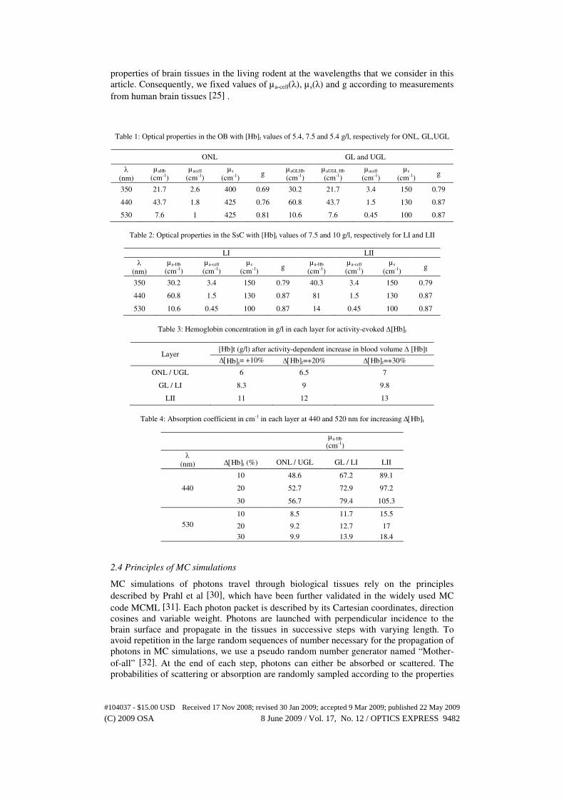
properties of brain tissues in the living rodent at the wavelengths that we consider in this

article. Consequently, we fixed values of µa-cell(λ), µ s(λ) and g according to measurements

from human brain tissues [25] .

Table 1: Optical properties in the OB with [Hb]t values of 5.4, 7.5 and 5.4 g/l, respectively for ONL, GL,UGL

ONL GL and UGL

λ

(nm)

µaHb

(cm-1)

µacell

(cm-1)

µ s

(cm-1) g

µaGLHb

(cm-1)

µaUGL Hb

(cm-1)

µacell

(cm-1)

µ s

(cm-1) g

350 21.7 2.6 400 0.69 30.2 21.7 3.4 150 0.79

440 43.7 1.8 425 0.76 60.8 43.7 1.5 130 0.87

530 7.6 1 425 0.81 10.6 7.6 0.45 100 0.87

Table 2: Optical properties in the SsC with [Hb]t values of 7.5 and 10 g/l, respectively for LI and LII

LI LII

λ (nm)

µa-Hb

(cm-1)

µa-cell

(cm-1)

µ s

(cm-1) g

µa-Hb

(cm-1)

µa-cell

(cm-1)

µ s

(cm-1) g

350 30.2 3.4 150 0.79 40.3 3.4 150 0.79

440 60.8 1.5 130 0.87 81 1.5 130 0.87

530 10.6 0.45 100 0.87 14 0.45 100 0.87

Table 3: Hemoglobin concentration in g/l in each layer for activity-evoked ∆[Hb]t

Layer [Hb]t (g/l) after activity-dependent increase in blood volume ∆ [Hb]t

∆[Hb]t= +10% ∆[Hb]t=+20% ∆[Hb]t=+30%

ONL / UGL 6 6.5 7

GL / LI 8.3 9 9.8

LII 11 12 13

Table 4: Absorption coefficient in cm-1 in each layer at 440 and 520 nm for increasing ∆[Hb]t

µa-Hb

(cm-1)

λ (nm) ∆[Hb]t (%) ONL / UGL GL / LI LII

440

10 48.6 67.2 89.1

20 52.7 72.9 97.2

30 56.7 79.4 105.3

530

10 8.5 11.7 15.5

20 9.2 12.7 17

30 9.9 13.9 18.4

2.4 Principles of MC simulations

MC simulations of photons travel through biological tissues rely on the principles

described by Prahl et al [30], which have been further validated in the widely used MC

code MCML [31]. Each photon packet is described by its Cartesian coordinates, direction

cosines and variable weight. Photons are launched with perpendicular incidence to the

brain surface and propagate in the tissues in successive steps with varying length. To

avoid repetition in the large random sequences of number necessary for the propagation of

photons in MC simulations, we use a pseudo random number generator named “Mother-

of-all” [32]. At the end of each step, photons can either be absorbed or scattered. The

probabilities of scattering or absorption are randomly sampled according to the properties



of the tissues and the Henyey Greenstein phase function. No Russian roulette termination

of photon was used to preserve the accuracy of MC simulations for the determination of

absorption coordinates. The geometry is semi infinite so that photons travelling deeper

than 1200 µm from the surface are no longer propagated and are considered as

“Transmitted” photons. The photons directly reflected by the surface and the photons

backscattered after having penetrated the tissues are both considered and counted as

“Reflected” photons. In our MC simulations 108 photons were launched to achieve

acceptable statistical accuracy on the recorded parameters

2.4.1 Absorption of excitation photons

For both SsC and OB models and for the wavelengths of excitation of NADH (350 nm)

[33] and Fp (440 nm) [34], the coordinates of absorbed photons were recorded. First, the

vascular absorption was studied using µa-Hb as absorption coefficient for both SsC and OB

models. Second, the total absorption for each layer, including absorption by cellular

fluorescent chromophores, was studied using µa as the total absorption coefficient. The

matrixes of vascular absorption probability and the matrixes of total absorption

probability were derived from these simulations.

2.4.2 Emission and detection of fluorescence photons

Fluorescence matrixes were obtained by subtracting the total hemoglobin matrix of

absorption from the total hemoglobin and tissues matrix of absorption. The resulting

matrices reflect the heterogeneous sources of fluorescence for the OB and SsC models

and were used as isotropic sources for either NADH or Fp fluorescence. In the absence of

in vivo data, a non-realistic fluorescence quantum efficiency of 1 was considered for both

NADH and Fp. Emitted photons were propagated in tissues and their coordinates and

direction cosines recorded after each step. Then, for each location in the 3-dimensional

models of OB and SsC, we derived the probability of a photon scattering to that location

from the functional layers GL and LII. Fluorescence photons detected are those exiting

the brain with a direction cosines encompassed within the numerical aperture of the

optical apparatus, which was set to 0.14.

3. Results

3.1 Absorption and backscattering of excitation photons at 350 and 440 nm in the SsC

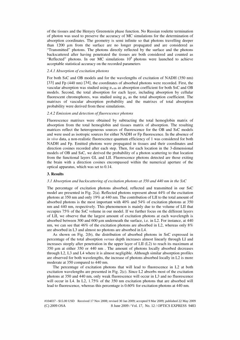
The percentage of excitation photons absorbed, reflected and transmitted in our SsC

model are presented in Fig. 2(a). Reflected photons represent about 44% of the excitation

photons at 350 nm and only 19% at 440 nm. The contribution of LII to the total amount of

absorbed photons is the most important with 40% and 54% of excitation photons at 350

nm and 440 nm, respectively. This phenomenon is mainly due to the volume of LII that

occupies 75% of the SsC volume in our model. If we further focus on the different layers

of LII, we observe that the largest amount of excitation photons at each wavelength is

absorbed between 300 and 600 µm underneath the surface, i.e. in L2. For instance, at 440

nm, we can see that 46% of the excitation photons are absorbed in L2, whereas only 8%

are absorbed in L3 and almost no photons are absorbed in L4.

As shown on Fig. 2(b), the distribution of absorbed photons in SsC expressed in

percentage of the total absorption versus depth increases almost linearly through LI and

increases steeply after penetration in the upper layer of LII (L2) to reach its maximum at

350 µm at either 350 or 440 nm . The amount of photons locally absorbed decreases

through L2, L3 and L4 where it is almost negligible. Although similar absorption profiles

are observed for both wavelengths, the increase of photons absorbed locally in L2 is more

moderate at 350 compared to 440 nm.

The percentage of excitation photons that will lead to fluorescence in L2 at both

excitation wavelengths are presented in Fig. 2(c). Since L2 absorbs most of the excitation

photons at 350 and 440 nm, only weak fluorescence will occur in L3 and no fluorescence

will occur in L4. In L2, 1.75% of the 350 nm excitation photons that are absorbed will

lead to fluorescence, whereas this percentage is 0.60% for excitation photons at 440 nm.



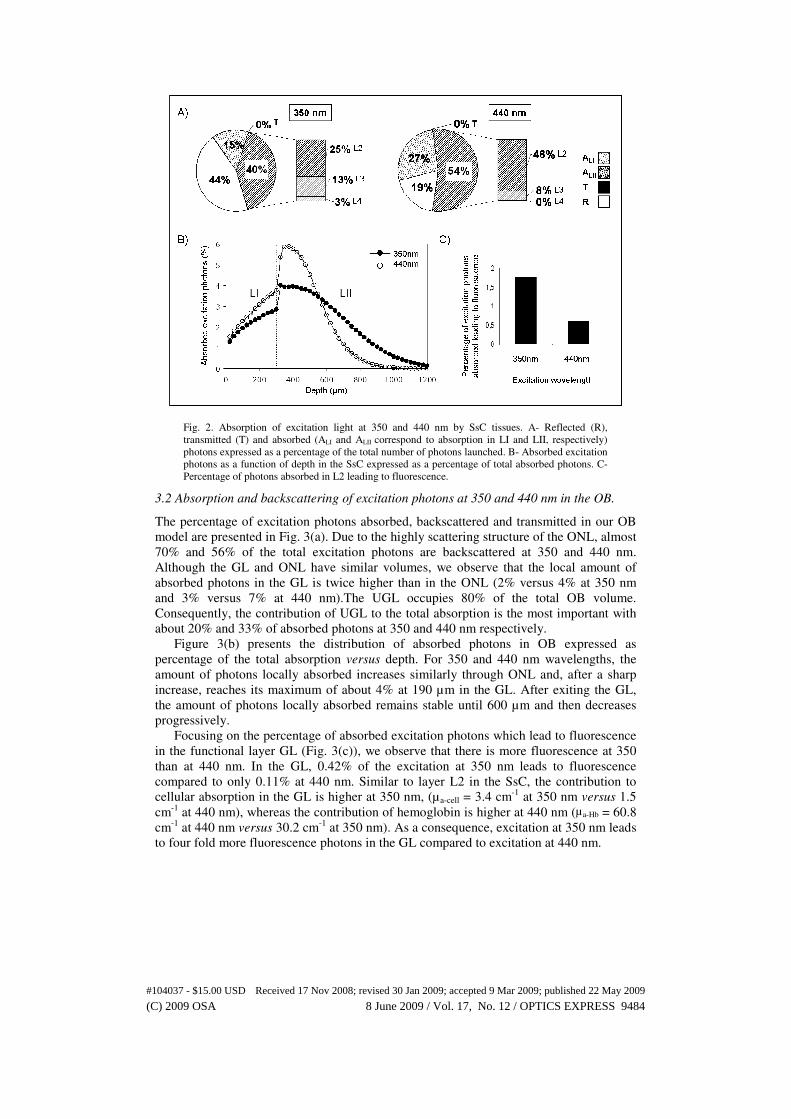
Fig. 2. Absorption of excitation light at 350 and 440 nm by SsC tissues. A- Reflected (R),

transmitted (T) and absorbed (ALI and ALII correspond to absorption in LI and LII, respectively)

photons expressed as a percentage of the total number of photons launched. B- Absorbed excitation

photons as a function of depth in the SsC expressed as a percentage of total absorbed photons. C-

Percentage of photons absorbed in L2 leading to fluorescence.

3.2 Absorption and backscattering of excitation photons at 350 and 440 nm in the OB.

The percentage of excitation photons absorbed, backscattered and transmitted in our OB

model are presented in Fig. 3(a). Due to the highly scattering structure of the ONL, almost

70% and 56% of the total excitation photons are backscattered at 350 and 440 nm.

Although the GL and ONL have similar volumes, we observe that the local amount of

absorbed photons in the GL is twice higher than in the ONL (2% versus 4% at 350 nm

and 3% versus 7% at 440 nm).The UGL occupies 80% of the total OB volume.

Consequently, the contribution of UGL to the total absorption is the most important with

about 20% and 33% of absorbed photons at 350 and 440 nm respectively.

Figure 3(b) presents the distribution of absorbed photons in OB expressed as

percentage of the total absorption versus depth. For 350 and 440 nm wavelengths, the

amount of photons locally absorbed increases similarly through ONL and, after a sharp

increase, reaches its maximum of about 4% at 190 µm in the GL. After exiting the GL,

the amount of photons locally absorbed remains stable until 600 µm and then decreases

progressively.

Focusing on the percentage of absorbed excitation photons which lead to fluorescence

in the functional layer GL (Fig. 3(c)), we observe that there is more fluorescence at 350

than at 440 nm. In the GL, 0.42% of the excitation at 350 nm leads to fluorescence

compared to only 0.11% at 440 nm. Similar to layer L2 in the SsC, the contribution to

cellular absorption in the GL is higher at 350 nm, (µa-cell = 3.4 cm-1 at 350 nm versus 1.5

cm-1 at 440 nm), whereas the contribution of hemoglobin is higher at 440 nm (µa-Hb = 60.8

cm-1 at 440 nm versus 30.2 cm-1 at 350 nm). As a consequence, excitation at 350 nm leads

to four fold more fluorescence photons in the GL compared to excitation at 440 nm.



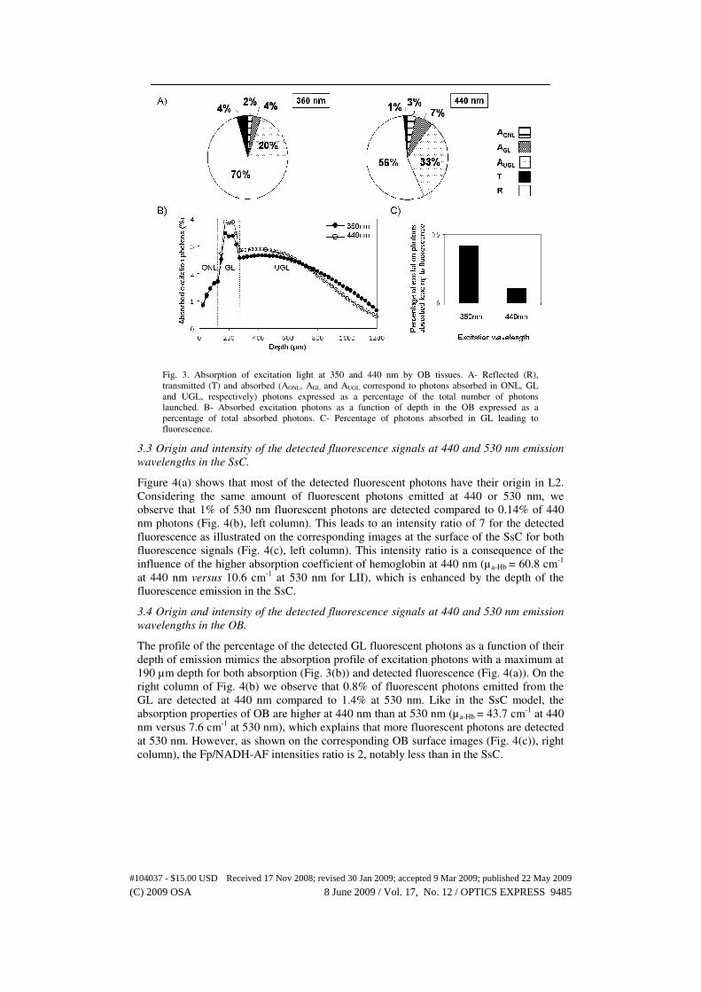
Fig. 3. Absorption of excitation light at 350 and 440 nm by OB tissues. A- Reflected (R),

transmitted (T) and absorbed (AONL, AGL and AUGL correspond to photons absorbed in ONL, GL

and UGL, respectively) photons expressed as a percentage of the total number of photons

launched. B- Absorbed excitation photons as a function of depth in the OB expressed as a

percentage of total absorbed photons. C- Percentage of photons absorbed in GL leading to

fluorescence.

3.3 Origin and intensity of the detected fluorescence signals at 440 and 530 nm emission

wavelengths in the SsC.

Figure 4(a) shows that most of the detected fluorescent photons have their origin in L2.

Considering the same amount of fluorescent photons emitted at 440 or 530 nm, we

observe that 1% of 530 nm fluorescent photons are detected compared to 0.14% of 440

nm photons (Fig. 4(b), left column). This leads to an intensity ratio of 7 for the detected

fluorescence as illustrated on the corresponding images at the surface of the SsC for both

fluorescence signals (Fig. 4(c), left column). This intensity ratio is a consequence of the

influence of the higher absorption coefficient of hemoglobin at 440 nm (µa-Hb = 60.8 cm-1

at 440 nm versus 10.6 cm-1 at 530 nm for LII), which is enhanced by the depth of the

fluorescence emission in the SsC.

3.4 Origin and intensity of the detected fluorescence signals at 440 and 530 nm emission

wavelengths in the OB.

The profile of the percentage of the detected GL fluorescent photons as a function of their

depth of emission mimics the absorption profile of excitation photons with a maximum at

190 µm depth for both absorption (Fig. 3(b)) and detected fluorescence (Fig. 4(a)). On the

right column of Fig. 4(b) we observe that 0.8% of fluorescent photons emitted from the

GL are detected at 440 nm compared to 1.4% at 530 nm. Like in the SsC model, the

absorption properties of OB are higher at 440 nm than at 530 nm (µa-Hb = 43.7 cm-1 at 440

nm versus 7.6 cm-1 at 530 nm), which explains that more fluorescent photons are detected

at 530 nm. However, as shown on the corresponding OB surface images (Fig. 4(c)), right

column), the Fp/NADH-AF intensities ratio is 2, notably less than in the SsC.



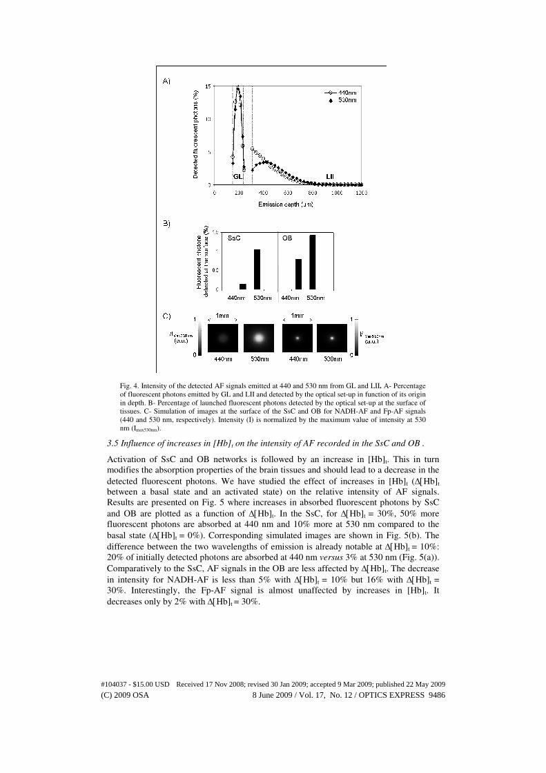
Fig. 4. Intensity of the detected AF signals emitted at 440 and 530 nm from GL and LII. A- Percentage

of fluorescent photons emitted by GL and LII and detected by the optical set-up in function of its origin

in depth. B- Percentage of launched fluorescent photons detected by the optical set-up at the surface of

tissues. C- Simulation of images at the surface of the SsC and OB for NADH-AF and Fp-AF signals

(440 and 530 nm, respectively). Intensity (I) is normalized by the maximum value of intensity at 530

nm (Imax530nm).

3.5 Influence of increases in [Hb]t on the intensity of AF recorded in the SsC and OB .

Activation of SsC and OB networks is followed by an increase in [Hb]t. This in turn

modifies the absorption properties of the brain tissues and should lead to a decrease in the

detected fluorescent photons. We have studied the effect of increases in [Hb]t (∆[Hb]t

between a basal state and an activated state) on the relative intensity of AF signals.

Results are presented on Fig. 5 where increases in absorbed fluorescent photons by SsC

and OB are plotted as a function of ∆[Hb]t. In the SsC, for ∆[Hb]t = 30%, 50% more

fluorescent photons are absorbed at 440 nm and 10% more at 530 nm compared to the

basal state (∆[Hb]t = 0%). Corresponding simulated images are shown in Fig. 5(b). The

difference between the two wavelengths of emission is already notable at ∆[Hb]t = 10%:

20% of initially detected photons are absorbed at 440 nm versus 3% at 530 nm (Fig. 5(a)).

Comparatively to the SsC, AF signals in the OB are less affected by ∆[Hb]t. The decrease

in intensity for NADH-AF is less than 5% with ∆[Hb]t = 10% but 16% with ∆[Hb]t =

30%. Interestingly, the Fp-AF signal is almost unaffected by increases in [Hb]t. It

decreases only by 2% with ∆[Hb]t = 30%.



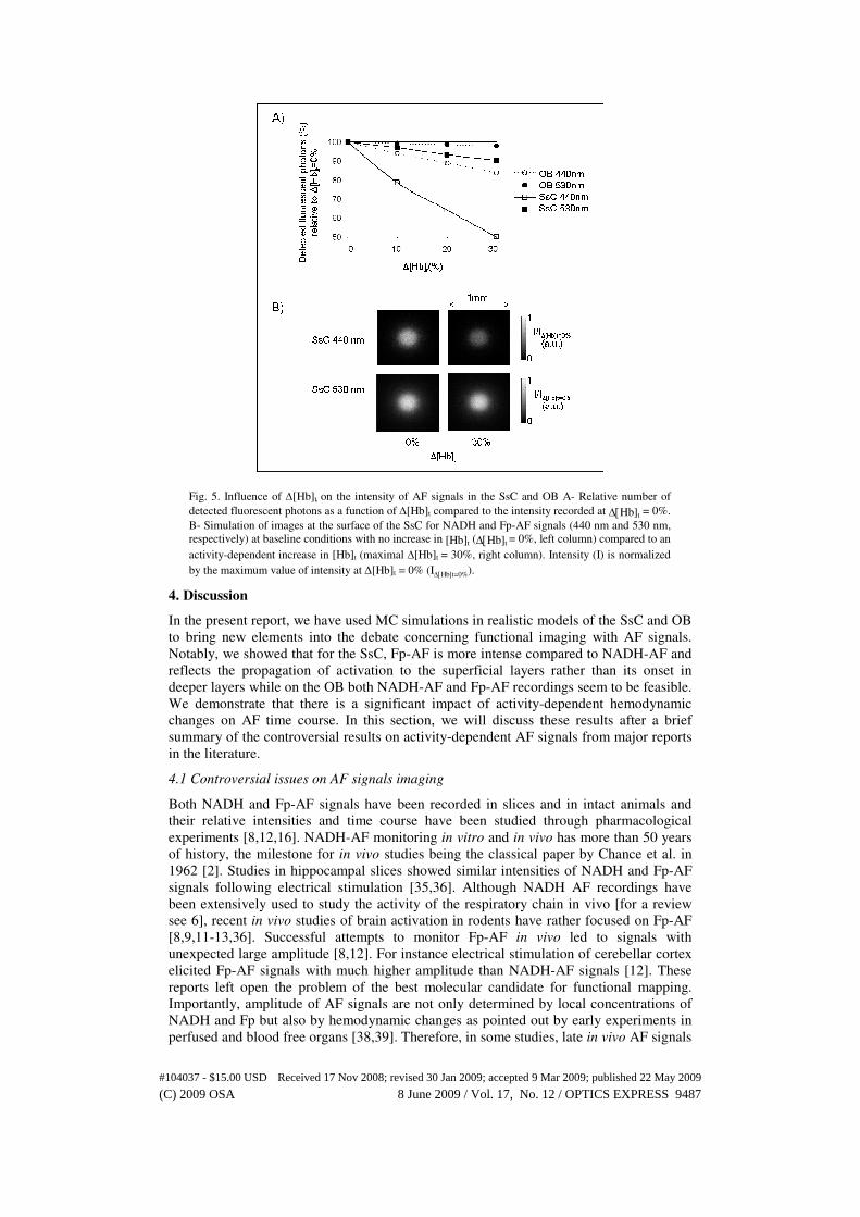
Fig. 5. Influence of ∆[Hb]t on the intensity of AF signals in the SsC and OB A- Relative number of

detected fluorescent photons as a function of ∆[Hb]t compared to the intensity recorded at ∆[Hb]t = 0%.

B- Simulation of images at the surface of the SsC for NADH and Fp-AF signals (440 nm and 530 nm,

respectively) at baseline conditions with no increase in [Hb]t (∆[Hb]t = 0%, left column) compared to an

activity-dependent increase in [Hb]t (maximal ∆[Hb]t = 30%, right column). Intensity (I) is normalized

by the maximum value of intensity at ∆[Hb]t = 0% (I∆[Hb]t=0%).

4. Discussion

In the present report, we have used MC simulations in realistic models of the SsC and OB

to bring new elements into the debate concerning functional imaging with AF signals.

Notably, we showed that for the SsC, Fp-AF is more intense compared to NADH-AF and

reflects the propagation of activation to the superficial layers rather than its onset in

deeper layers while on the OB both NADH-AF and Fp-AF recordings seem to be feasible.

We demonstrate that there is a significant impact of activity-dependent hemodynamic

changes on AF time course. In this section, we will discuss these results after a brief

summary of the controversial results on activity-dependent AF signals from major reports

in the literature.

4.1 Controversial issues on AF signals imaging

Both NADH and Fp-AF signals have been recorded in slices and in intact animals and

their relative intensities and time course have been studied through pharmacological

experiments [8,12,16]. NADH-AF monitoring in vitro and in vivo has more than 50 years

of history, the milestone for in vivo studies being the classical paper by Chance et al. in

1962 [2]. Studies in hippocampal slices showed similar intensities of NADH and Fp-AF

signals following electrical stimulation [35,36]. Although NADH AF recordings have

been extensively used to study the activity of the respiratory chain in vivo [for a review

see 6], recent in vivo studies of brain activation in rodents have rather focused on Fp-AF

[8,9,11-13,36]. Successful attempts to monitor Fp-AF in vivo led to signals with

unexpected large amplitude [8,12]. For instance electrical stimulation of cerebellar cortex

elicited Fp-AF signals with much higher amplitude than NADH-AF signals [12]. These

reports left open the problem of the best molecular candidate for functional mapping.

Importantly, amplitude of AF signals are not only determined by local concentrations of

NADH and Fp but also by hemodynamic changes as pointed out by early experiments in

perfused and blood free organs [38,39]. Therefore, in some studies, late in vivo AF signals



(>2s after stimulation onset) were considered to be affected by increase in blood flow

following stimulation [8,13]. Contrarily, on the basis of pharmacological experiments,

Reinert et al. [8] supported the idea that “hemoglobin absorption and changes in blood

flow do not contribute significantly to the AF signal” [12]. Thus, another key issue

dealing with the interference of hemodynamics with AF signals time course has to be

quantitatively discussed.

4.2 Which is the best candidate for AF functional mapping : NADH or Fp?

The yield of the complete imaging process (i.e. fluorescence excitation and detection)

depends on several anatomical and physiological parameters, which have opposite effects

on AF signals. Indeed, optical absorption and scattering properties are directly related to

the vascularization of the tissues, the density of highly scattering structures, and the

dimension and depth of the functional area. Regarding the distribution of the fluorescence

sources within the layers, it is related to the distribution of mitochondria where most of

the NADH fluorescence occurs and where the Fp are located. Although literature on the

mitochondria density in brain tissues is sparse, it is well known that the mitochondria

concentration is high at the pre-synaptic and post-synaptic locations where the energy

demand is high. The depth and extension of the locations with high synaptic density,

hence high NADH and Fp concentrations, vary from one brain structure to another.

Considering all these anatomofunctionnal parameters for the OB where AF recordings

have not been reported so far, it is not straightforward to state whether such recording will

be feasible in vivo. In the OB, the dense micro-vascularization of functional units results

in higher absorption properties than in surrounding tissues. In addition, the superficial

location of the functional units in the OB a priori favorable to optical recordings is

counterbalanced by the high scattering properties of the first layer (ONL) which lead to a

large amount of backscattered light and consequently limit photons penetration and

fluorescence excitation in the OB. Finally, the small dimensions of the functional units in

the OB leads to a lower absolute number of emitted fluorescence photons compared to

those emitted from the very large volume of the neocortical column in the SsC. However,

considering an optical apparatus with a thin optical section (high NA objective with wide-

field epi-fluorescence, or two-photon excitation) one might expect very similar detection

abilities from regions with similar properties in terms of optical properties and

mitochondrial density. The MC simulations allow integrating all these effects for AF

recordings in the SsC and OB. Regarding the location of the detected AF signals, the

results for the SsC are in agreement with previous findings in SsC coronal slices showing

that the maximum intensity of fluorescence was located in L2 around a cortical depth of

300µm [8]. In the OB, MC simulations show that the maximum fluorescence intensity is

found in the GL around a 190µm depth. This is in good agreement with functional MRI

studies [40] and 14

C-2-DG autoradiography studies [41], which have shown that most of

the energy-related signals detected in the OB are located in the GL.

Further investigations of the MC results allow quantifying the expected relative intensities

of NADH-AF and Fp–AF in both structures. Considering simulated intensities ratios, the

absorption properties of blood in brain tissues (table 1 and 2) are more favorable to

NADH excitation compared to Fp-AF but more favorable to Fp-AF emission compared to

NADH. To evaluate the influence of the absorption from blood we have considered the

overall process with its 4 successive steps i) propagation of excitation photons to the

endogenous fluorophores, ii) fluorescence with a quantum yield η, iii) propagation of

fluorescence photons and iv) detection of exiting photons. Our simulations confirm that

NADH excitation is favored compared to Fp excitation in the SsC (Fig. 2(c)) and OB

(Fig. 3(c)) with ratios of 3 and 4 between the cellular absorption at 350 and 440 nm

respectively. Although quantum yields are likely to be affected by physiological

conditions (pH, ions, molecular conformation), to our knowledge only in vitro values are

available for NADH and Fp and are respectively 0.019 and 0.025 [42]. The third and last

steps of the process were combined in the second series of MC simulations. The results

(Fig. 4(a)) showed a pronounced advantage for Fp-AF in SsC (ratio of 7) and less

pronounced but yet significant advantage for Fp-AF in the OB (ratio of 2). Considering



the whole process including the quantum yield, simulations show a ratio of 3.4 in favor of

the Fp-AF in the SsC and a ratio of 1.6 in favor of NADH in the OB. It is noticeable that

for the SsC the ratio of Fp-AF to NADH-AF intensities derived from our simulations is

comparable to that observed experimentally in vivo [7]. In addition, as already observed

with other intrinsic optical signals [43] our results point out that AF intensity varies from

one brain region to another. Considering the basal hemodynamics of these structures, our

simulations show that in terms of intensities, the Fp signal is the best choice for in vivo

functional imaging in the SsC whereas NADH-AF and Fp-AF are both good candidates

for AF recordings in the OB.

4.3 Do hemodynamics interfere with AF signals time course?

The time course of AF signals was studied in brain slices 2 [8,16] as well as in vivo [8,12]

and was shown to be related to the duration and intensity of the stimulation. All studies

have shown biphasic profiles for AF signals, which are attributed to changes in the redox

states of NADH and Fp. After stimulation onset, Fp-AF and NADH-AF present inversed

temporal profiles with an initial rapid decrease of NADH-AF (corresponding to a fast Fp-

AF increase) followed by a slow increase of NADH-AF intensity (corresponding to a

slow Fp-AF decrease). To study the influence of hemodynamics on the time course of AF

signals, we have simulated the activation-induced transient increase in blood flow [44],

which affects the optical properties of tissues. It is important to note that the time course

of hemodynamic changes is much slower compared to that of AF signals, which are more

closely related to electrical transmission [8,12]. In the SsC, the maximum ∆[Hb]t was

reported to occur 2 to 3 seconds following the end of a 1 second electrical stimulation

[26-29,44,45]. In the OB, an increase in blood flow was observed about 2 seconds after

olfactory stimulation onset [15,21]. Considering our simulations, we can assume that the

AF-signals are almost left unaffected by hemodynamic changes during the first 1-2

seconds following activation (corresponding to ∆[Hb]t of about 10-20%) except for

NADH–AF in the SsC. Considering longer delays after stimulation onset, an important

proportion of fluorescent photons is absorbed due to increase in optical absorption of the

tissues. As expected from the absorption properties of blood, the effect is much stronger

for NADH than for Fp. It is also much stronger in the SsC than in the OB since

fluorescent photons have to travel for a longer path in the SsC compared to OB. In vivo

experiments where hemodynamic changes were blocked by nitric oxide synthase

inhibitors have been carried out to separate AF from subsequent hemodynamic responses,

but have led to different conclusions. On the one hand, Reinert et al. (2004) showed that

in the cerebellar cortex L-nitroarginine-methyl ester does not affect Fp-AF intensities at

different stimulation conditions (n = 3, Fig. 9 and Fig. 10 within [12]). On the other hand,

Shibuki et al. showed that Fp-AF signals recorded under NG-nitro-L-arginine challenge

are about twice more intense compared to the control experiment. In the same study the

second phase of the AF signals is temporally delayed by one second (Fig. 7(a) and Fig.

7(d) in [8]). In the SsC, our results lean towards the findings of Shibuki et al. since they

show that for ∆[Hb]t = 30% about 10% of the signal is absorbed for Fp-AF and about 50%

for NADH–AF. Furthermore, in some experiments in the SsC, the Fp-AF signals reach

their maximum and start to decrease before the end of the stimulation [13], which implies

that Fp-AF signals are affected by hemodynamic changes within seconds following

stimulation onset. Our results support and quantify these findings and the methodological

choice made by Weber et al [13] to exclude the late phase (>2s after stimulation onset)

from the Fp-AF recordings to map brain activation accurately.

5. Conclusion

Using MC simulations of AF signals in realistic models of the rat SsC and OB, we found

that the feasibility of AF recordings in different brain areas is highly dependent on local

and specific anatomofunctional features. For the SsC, we showed that Fp-AF signal is

significantly more intense compared to NADH-AF in agreement with previous studies

carried out in vivo. Thus, the Fp signal is the best choice for in vivo functional imaging in

the SsC whereas NADH-AF and Fp-AF are both good candidates for AF recordings in the



OB. In addition, we demonstrated that Fp-AF recordings in the SsC reflect the

propagation of activation to the superficial layers rather than its onset in deeper layers.

Finally, our simulations allowed quantifying the influence of hemodynamics on AF

signals intensities and time course. Consequently, to obtain accurate activation maps

using AF signals it is important to carefully consider the contamination of AF signals by

subsequent hemodynamic changes especially for AF-Fp imaging in deep structures.

Acknowledgments

This work was supported by ANR grant ANR-06-NEURO-004-01/Astroglo and the BQR

program from Université Paris Diderot - Paris VII. Ph-D scholarship of B. L’Heureux is

funded by CNRS-IN2P3. We thank Dr C. Martin for helpful comments on the manuscript.



Documents

Autofluorescence imaging of NADH and flavoproteins in the rat brain: insights from Monte Carlo simulations