Calhoun: The NPS Institutional ArchiveDSpace Repository

Theses and Dissertations 1. Thesis and Dissertation Collection, all items

1971

Parameter plane study of the optimal regulator.

Swett, Lionel Alfonso Doren.Monterey, California ; Naval Postgraduate School

http://hdl.handle.net/10945/15848

Downloaded from NPS Archive: Calhoun

PARAMETER PLANE STUDY OFTHE OPTIMAL REGULATOR

Lionel Alfonso Doren Swett

DUDLEY

liAVAL P( JHOOLMONTEREY, Ul., A 93943-50ttj

DUDLEY r -Y

IWVAL PC SCHOOLMONTEREY. u..„_hIA 93943-5001

United StatesNaval Postgraduate School

THEPARAMETER PLANE STUDY OF

THE OPTIMAL REGULATOR

by

Lionel Alfonso Doren Swett

Thesis Advisor: G.J. Thaler

tlUN M I<J r

Approved ^o-t public ticlzcLid.; dU>txibuution LuitimiXzd.

Parameter Plane Study of the Optimal Regulator

by

Lionel Alfonso Doren SwettTeniente Primero, Armada de Chile

Submitted in partial fulfillment of therequirements for the degree of

MASTER OF SCIENCE IN ELECTRICAL ENGINEERING

from the

NAVAL POSTGRADUATE SCHOOLJune 1971

ABSTRACT

Parameter plane studies of an optimal second order

regulator are presented. Emphasis is placed on the

interpretation of the cost function and the sensitivity of

the cost function to plant parameter incremental varia-

tions . An analysis is made of cost function weighting

factors and their effect on damping, speed of response,

and cost.

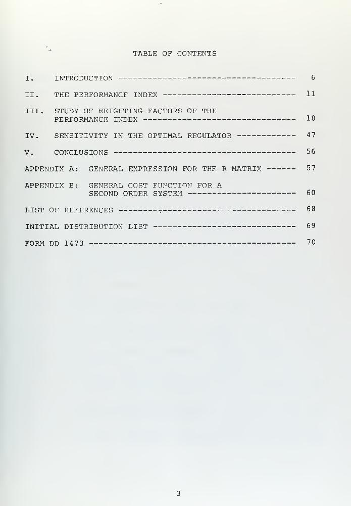
TABLE OF CONTENTS

I. INTRODUCTION 6

II. THE PERFORMANCE INDEX 11

III. STUDY OF WEIGHTING FACTORS OF THEPERFORMANCE INDEX 18

IV. SENSITIVITY IN THE OPTIMAL REGULATOR 47

V. CONCLUSIONS 56

APPENDIX A: GENERAL EXPRESSION FOR THF R MATRIX 57

APPENDIX B: GENERAL COST FUNCTION FOR ASECOND ORDER SYSTEM 60

LIST OF REFERENCES 68

INITIAL DISTRIBUTION LIST 69

FORM DD 1473 70

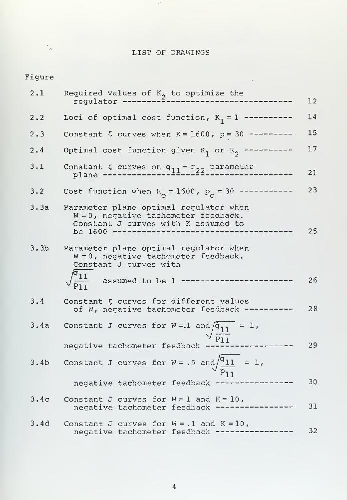
LIST OF DRAWINGS

Figure

2.1 Required values of K_ to optimize theregulator 12

2.2 Loci of optimal cost function, K.. = 1 14

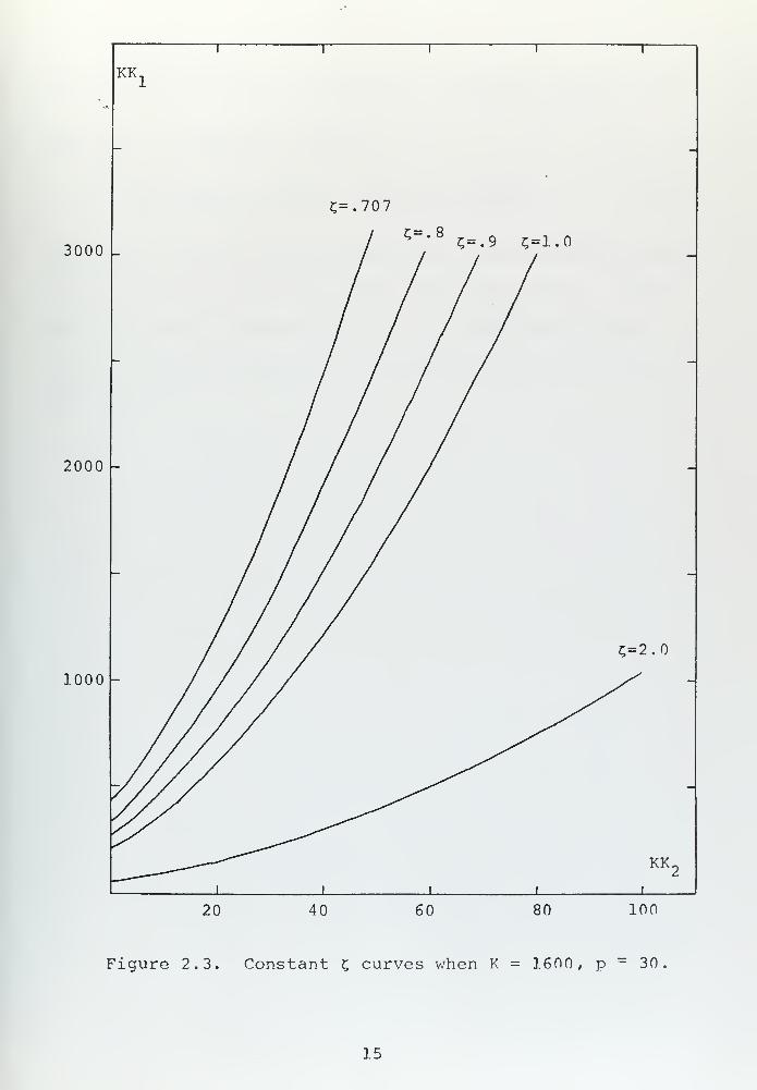
2.3 Constant C curves when K=1600, p=30 15

2.4 Optimal cost function given K. or K^ 17

3.1 Constant C curves on q, , - q^- parameterplane 2.1

3.2 Cost function when K =1600, p = 30 23o ^o

3.3a Parameter plane optimal regulator whenW=0, negative tachometer feedback.Constant J curves with K assumed tobe 1600 25

3.3b Parameter plane optimal regulator whenW=0, negative tachometer feedback.Constant J curves with

/ assumed to be 1 26v Pll

3.4 Constant £ curves for different valuesof W, negative tachometer feedback 28

3.4a Constant J curves for W =.1 and /q.1

= 1,

Pllnegative tachometer feedback 29

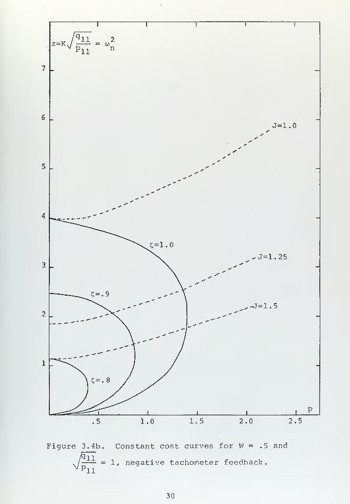
3.4b Constant J curves for W= .5 and/q ll = 1,

negative tachometer feedback 30

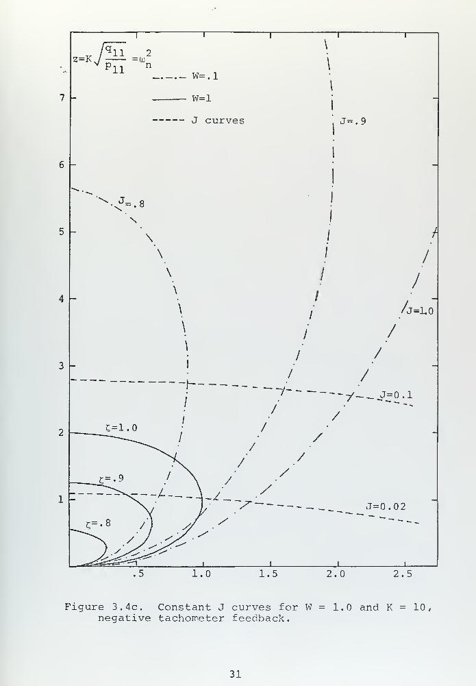
3.4c Constant J curves for W= 1 and K= 10,negative tachometer feedback 31

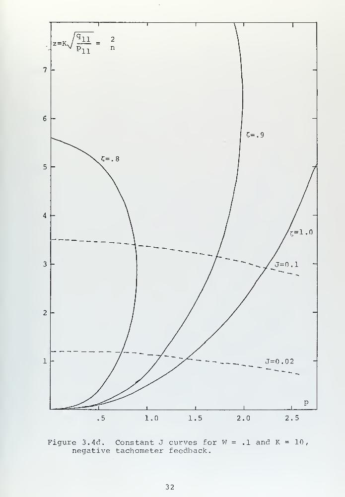
3.4d Constant J curves for W=.l and K=10,negative tachometer feedback 32

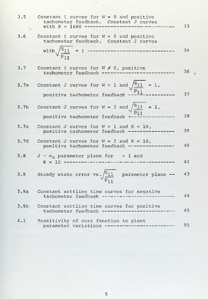
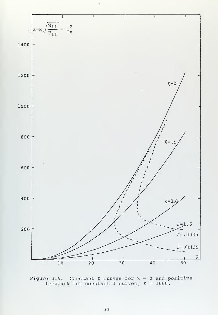
3.5 Constant £ curves for W = and positivetachometer feedback. Constant J curveswith K = 1600 33

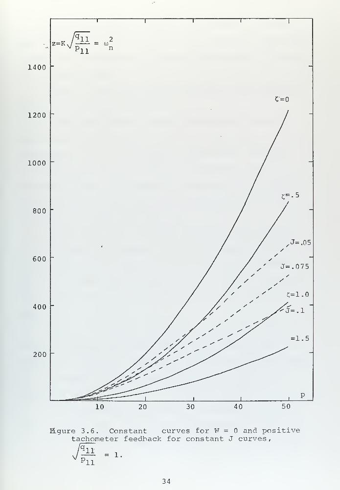
3.6 Constant ? curves for W = and positivetachometer feedback. Constant J curves

with /q ll = 1 34

3.7 Constant ? curves for W ^ 0, positivetachometer feedback 36T

3.7a Constant J curves for W = 1 and /*11 = 1,

pllpositive tachometer feedback 37

3.7b Constant J curves for W = 2 and /^ll = 1,

Pllpositive tachometer feedback 38

3.7c Constant J curves for W = 1 and K = 10

,

positive tachometer feedback 39

3.7d Constant J curves for W = 2 and K = 10

,

positive tachometer feedback 40

3.8 J - con parameter plane for = 1 and

K = 10 41

3.9 Steady state error vs . r*ll parameter plane — 43

3.9a Constant settling time curves for negativetachometer feedback 44

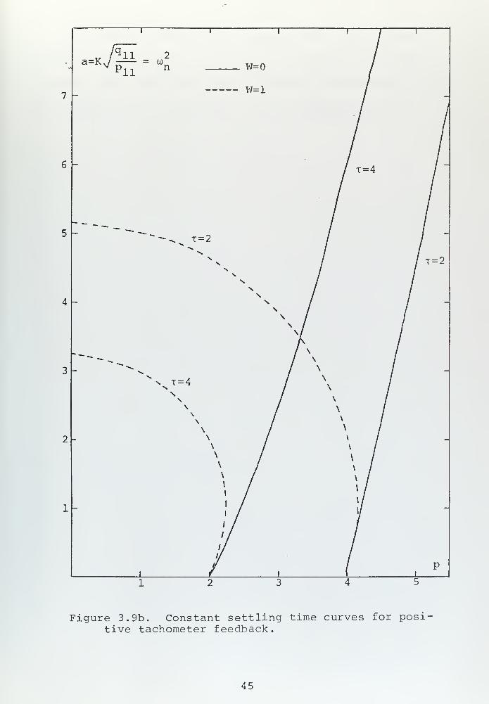
3.9b Constant settling time curves for positivetachometer feedback 45

4.1 Sensitivity of cost function to plantparameter variations 55

I. INTRODUCTION

The parameter plane study of an optimal regulator was

undertaken with the purpose of finding an interpretation of

the meaning of the cost function and of the weighting fac-

tors as they relate to the observed physical behaviour of

the regulator.

Chapter one gives a brief description of the problem

formulation; Chapter two describes some studies on the

performance index; Chapter three deals with the study of

the weighting factors , and Chapter four with some sensi-

tivity aspects. Appendices A and B deal with the develop-

ment of the general expression for the R matrix and the

performance index.

A. PROBLEM FORMULATION

Suppose that initially the plant input or any of its

derivatives is nonzero. Provide a plant input to bring the

output or its derivatives to zero. In other words, the

problem is to apply a control to take the plant from a

nonzero state to the zero state. This problem may occur

where the plant is subjected to unwanted disturbances that

perturb its output (e.g., a radar antenna control system

with the antenna subject to wind gusts)

.

The desirable properties of a regulator system should

be

:

A. The regulator system should involve a linear

control law.

B. By definition an optimal system is one that mini-

mizes a certain cost.

To achieve property B, let us define a performance index

00

PI = / (XTQX + u

TPu) dt

o

where Q is symmetric positive definite and R is a positive

00

Tdefinite matrix. / X QX dt come from the minimum integral-

square error problem.

00 J^ oo

/ Z (X.)2

dt = / (XTX) dt

o i=l1

o

constituting a reasonable measure of the system transient

oo

Tresponse, and ; u Pu dt comes from the minimum energy

o

problem.

The minimization problem, i.e., the task of finding

an optimal control that minimizes the performance index,

turns out to be achievable with a linear feedback law. This

is the reason why the performance index includes a measure

control energy.

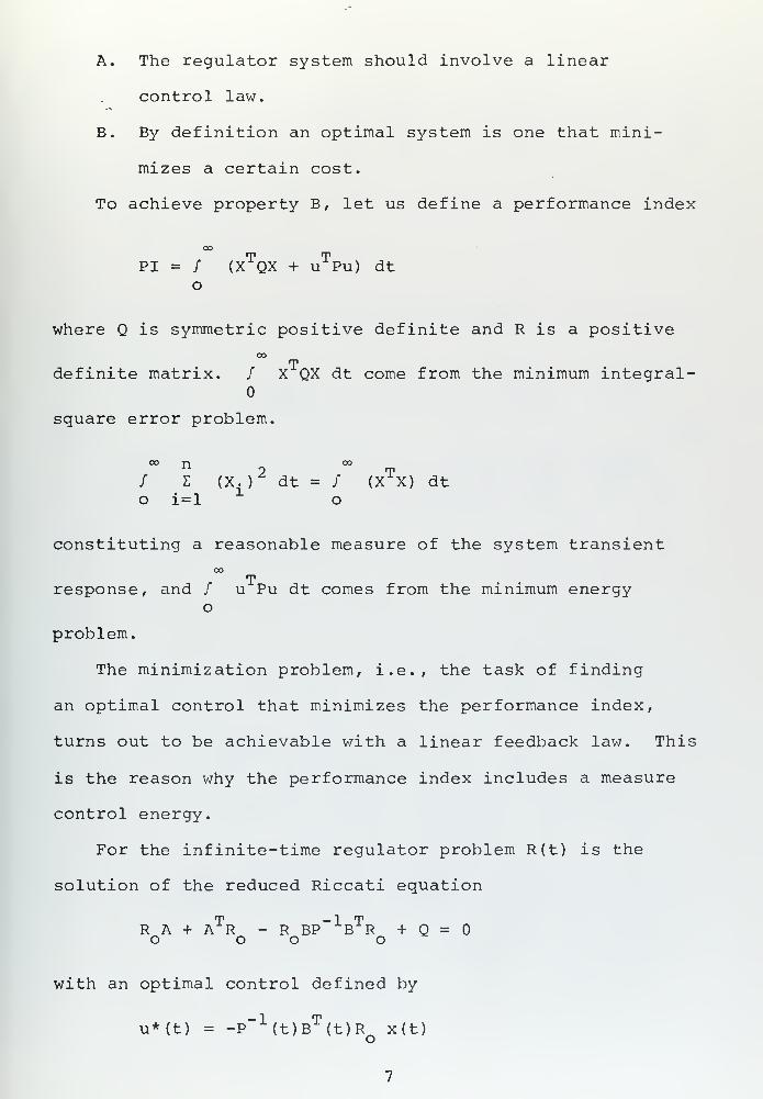
For the infinite-time regulator problem R(t) is the

solution of the reduced Riccati equation

R A + ATR - R BP~ 1BTR + Q =

o o o o

with an optimal control defined by

u*(t) = -P_1

(t)BT(t)R

ox(t)

where

A =1

[0 -P<

, AT =1 -pj

B = T, B

1= K

K _ tm _

R =o

rll

r12

r T12 22

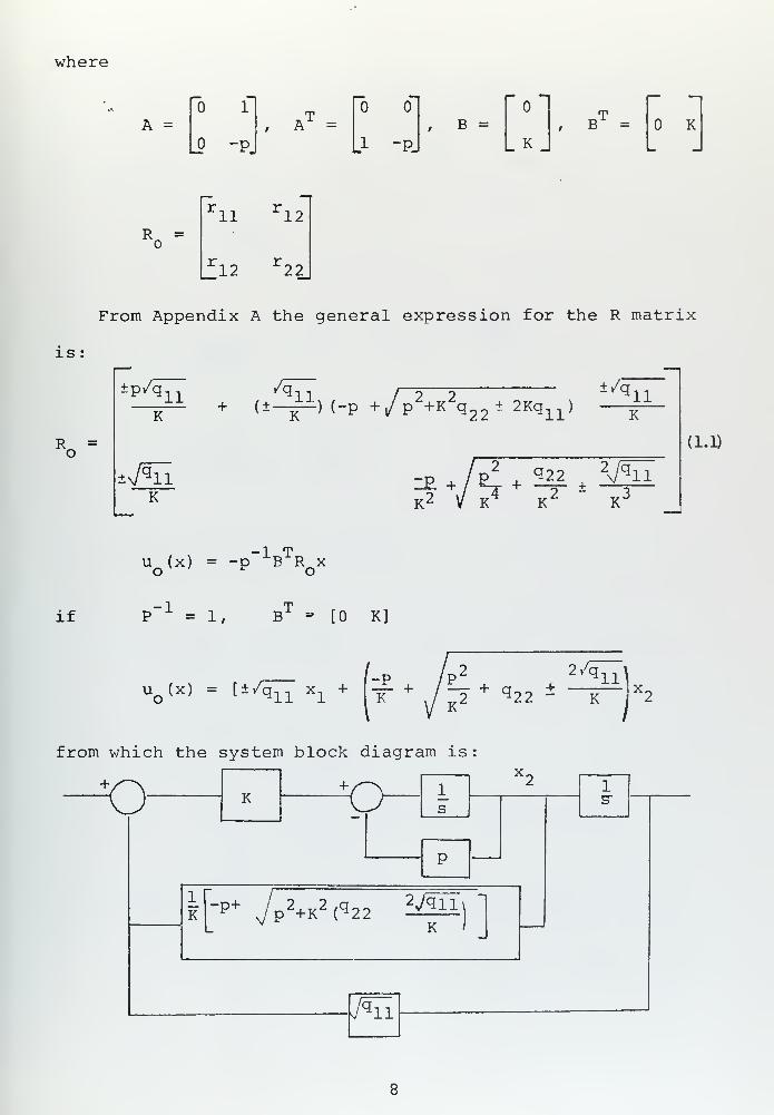
From Appendix A the general expression for the R matrix

is

Ro

"

ip^n ^q

K+ (^^X

1) ("P +/p 2

+K2q 22

± 2Kqi;L

)

/q 11K

±7511K K2 V K* K

2K3

(1.1)

U (x) = -p~ 1BTR x

o c o

if P-1 = 1, B

T - [0 K]

P2 2/q llV X) X

l+

\t~+7^2

+ q 22 * -IT"

from which the system block diagram is

:

+. "AK

+o 1

s

X2 1

5"J

P

1

K ~P+ 7p 2+K 2(q 22

2^qiiv

K '

/qn iV

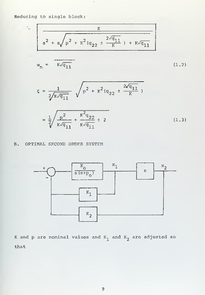
Reducing to single block:

K

2 „2 2/q11

s" + s,/ p" + K"(q22

± j^- ) + K/qi:L

0)n

= K/q11

(1.2)

C =2/K^ll

2 22v/5ll

p+ K (q 22

± ^r1 >

= 1 /jd 2.

K g2 :

+ — ± 2

K/gll

K/qll

(1.3)

B. OPTIMAL SECOND ORDER SYSTEM

"VKo

X1

c

a2

J s (s+pQ )

Kl

K2

K and p are nominal values and K, and K~ are adjusted so

that

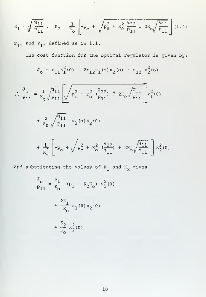
Kl -

i/ p

11

11'

K2 ~ K P +

2 q22PO + K

p± 2K

Lll

11Oi/ P 11

(1.4)

r, , and r, _ defined as in 1.1.

The cost function for the optimal regulator is given by:

Jo

= rnxi(°>

+ 2r12

x1(o)x

2(o) + r

22x*(o)

11

'11 O V ^11

2 2 q 22 + /qp^ + KZ {-^-) ± 2K /-

^o op,, of p

11

11x^(0)

+ W^I Xl(o>V°>

K'P +^o

2 2 q 22p + IT (-^) + 2K

11o q 11 oi/ p11

x*(0)

And substituting the values of K, and K~ gives

J K~£- = it- (P + K K ) x?(0)pll K

o ° 2 ° 1

2K+ -rf- x, (0)x 9 (0)

Ko

K2 2

o

10

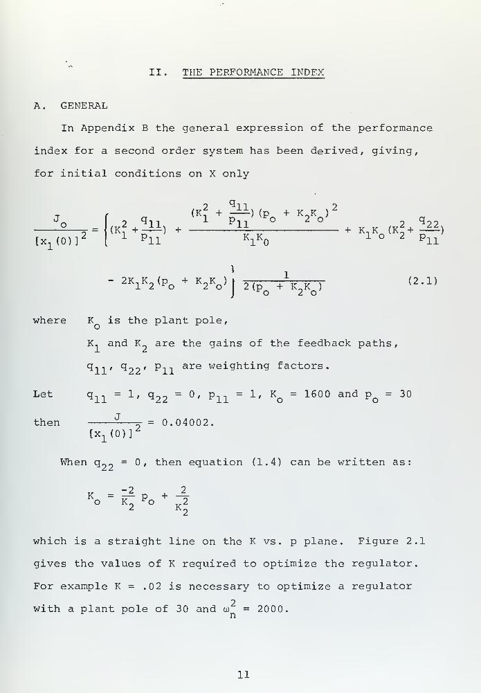
II. THE PERFORMANCE INDEX

A. GENERAL

In Appendix B the general expression of the performance

index for a second order system has been derived, giving,

for initial conditions on X only

Jo

[x.^0)]2

2 ^11 2(Kf + -±±) (p + K_K )

£

2 q ll 1 P1;L

O 2 o2 q

(K7 +^t±) + ±± + k,K (ld + -z±.)1 PU K lK() 1 o^ 2 pn '

- 2K,K_(p^ + K„K ) \ =-7,

1T>

-,1 2 ^o 2 o 2 (p + K-K )

J ^o 2 o(2.1)

where K is the plant pole,

K, and K« are the gains of the feedback paths,

q.., q ?:?/ p.,-, are weighting factors.

Let q,, = 1, q 22= 0, p, , = 1, K = 1600 and p = 30

then y = 0.04002.[x

1(0)]^

When q„» = 0, then equation (1.4) can be written as:

-2 2

° K2 ° K

2

2

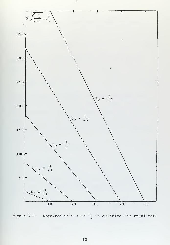
which is a straight line on the K vs . p plane. Figure 2.1

gives the values of K required to optimize the regulator.

For example K = .02 is necessary to optimize a regulator

2with a plant pole of 30 and oo = 2000.

11

3500-

3000-

2500"

2000 "

150C-

1000-

50C-

Figure 2.1. Required values of K_ to optimize the regulator.

12

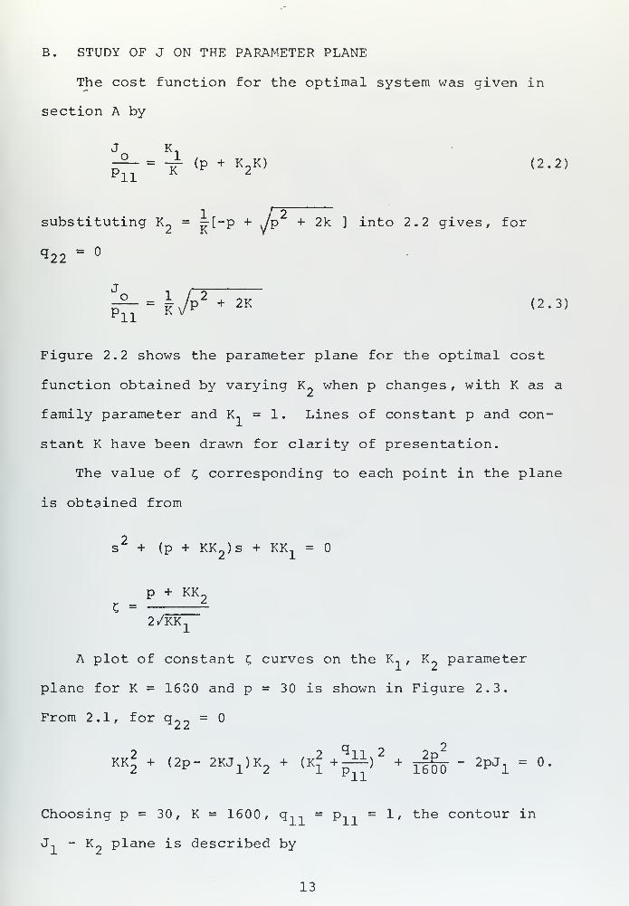
B. STUDY OF J ON THE PARAMETER PLANE

The cost function for the optimal system was given in

section A by

_2_ = J, (p + k2K) (2.2)

i nsubstituting K2

= ~[-p + JV + 2k ] into 2.2 gives, for

q 22 =

= i /p2

+ 2K (2.3)Pll K

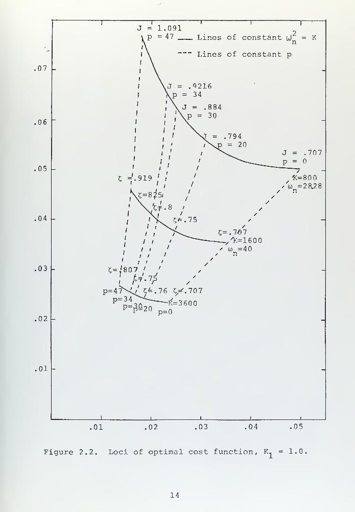
Figure 2.2 shows the parameter plane for the optimal cost

function obtained by varying K~ when p changes , with K as a

family parameter and K, = 1 . Lines of constant p and con-

stant K have been drawn for clarity of presentation.

The value of £ corresponding to each point in the plane

is obtained from

s2

+ (p + KK )s + KK, =

p + KK5 = -———±

2/KK,

A plot of constant £ curves on the K, , K~ parameter

plane for K = 16C0 and p = 30 is shown in Figure 2.3.

From 2.1, for q 2?=

2

'11KK

2+ (2P~ 2KJ

i)K

2+ (K

i+ E77

)2 +ifoo - 2 PJ i

=

Choosing p = 30, K = 1600, q, , = p, , =1, the contour in

J, - K_ plane is described by

13

07 -

06

05

04

03

J = 1.091

C ='.919 ' ,' '

£=8^5/

.' VkT.8 /

-K=800/to = 2 8.2 8

• n

/

£=.7<07^=1600

02

p=4 7vv'/ £=.76 C/^.707

P=^o|^ l(=3 600P^-2° p=0

01

01 02 03 04 .05

Figure 2.2. Loci of optimal cost function, K, = 1.0

14

3000 _

2000 -

1000

Figure 2.3. Constant X, curves when K = 1600, p - 30

.

15

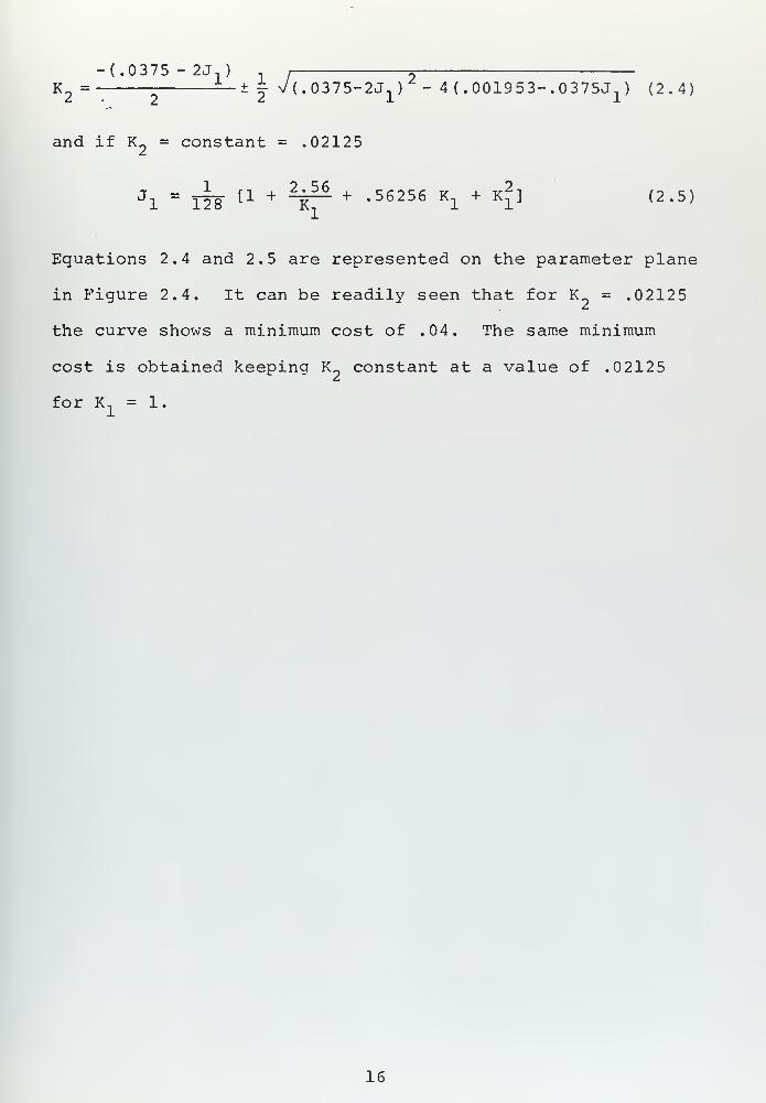
-(.0375 - 2J,

)

K2= -2L + | V(.0375-2J

1)

2- 4 (.001953-. 0375J

1) (2.4)

and if K„ = constant = .02125

Jl

=I2T [1 +

^T^"+ - 56256 K

i+ K

i ] < 2 - 5 )

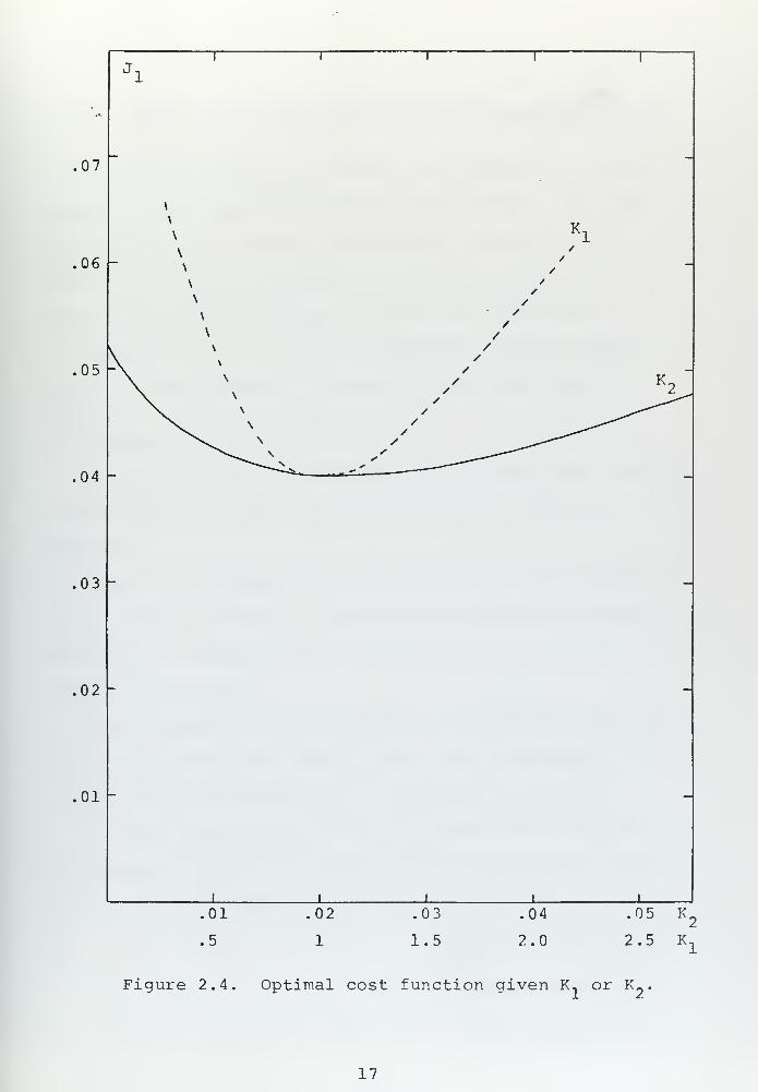
Equations 2.4 and 2.5 are represented on the parameter plane

in Figure 2.4. It can be readily seen that for K?

= .02125

the curve shows a minimum cost of .04. The same minimum

cost is obtained keeping K^ constant at a value of .02125

for K, = 1.

16

'«

Jl

i ! 1 1 1

07

\

\

\

\

Ki

•

06 \

\

\

\

\

\

//

//

//

//

//

05 —

\

\

/ —\ / K~\

//

2

s. \ />v \^^ \ • _^-^

—

X^ \ s _^»

—

"•

n^—

04• —-~*~^

03 -

02 -

01 -

11 1 1

i

.01 .02 .03 .04 .05 K

.5 1 1.5 2.0 2.5 K

Figure 2.4. Optimal cost function given K. or K„

17

III. STUDY OF WEIGHTING FACTORS OF THE PERFORMANCE INDEX

When it is desired to optimize the design of a control

system, a cost functional must be established. This cost

functional is an analytical expression, related to the

system, which must be minimized by choosing parameters

which will cause an extremal of the cost functional.

Weighting factors used in performance indices deter-

mine to a large extent the optimal system which results

.

A. SELECTION OF THE Q MATRIX

Optimal control law determination by Athans and Falb [1]

require that the weighting factors matrix be positive

definite.

Tuel [2] developed a canonical form for the weighting

factor matrix Q which has the minimum number of parameters

required in the performance index for the computation of the

optimal control law.

The selection of this Q matrix is a very important part

of optimal design but there is very little guidance in the

literature in the selection of the weighting factors.

In any regulator the output or "controlled variable" is

of primary interest and certainly must be weighted, being

never negative. Then

"11 " °

The velocity (x„ = x. ) need not be weighted at all

but certainly any weight attributed to the velocity will

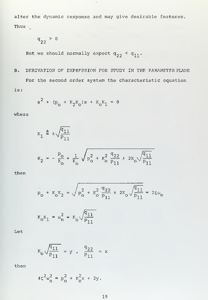
alter the dynamic response and may give desirable features

Thus •

q >M22

But we should normally expect q„,, < q,

,

B. DERIVATION OF EXPRESSION FOR STUDY IN THE PARAMETER PLANE

For the second order system the characteristic equation

is :

S2

+ (p + K K )s + K K, =0^o 2 o o 1

where

1 V P 1X

Po 1 / 2 v2 q 22 OL, v /qll

K_ = - it— + —-v/p +K ± 2K \/2 K K v ^O O p, , O v p,,o o *ll *ll

then

/ 2 2 q 22 /q il

p + K K„ = v/p + K -^ ± 2K J-^ = 2^00*o o 2 V ^o o p.., p lln

2 /q l]

K K, = co = Ko 1 n o ^ p11

Let

then

,

[H q 22

pll p ll

4c2

co2

= p2

+ K2x + 2y.n ^o o 2

19

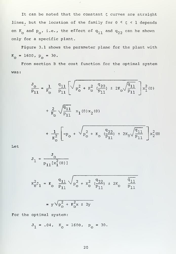
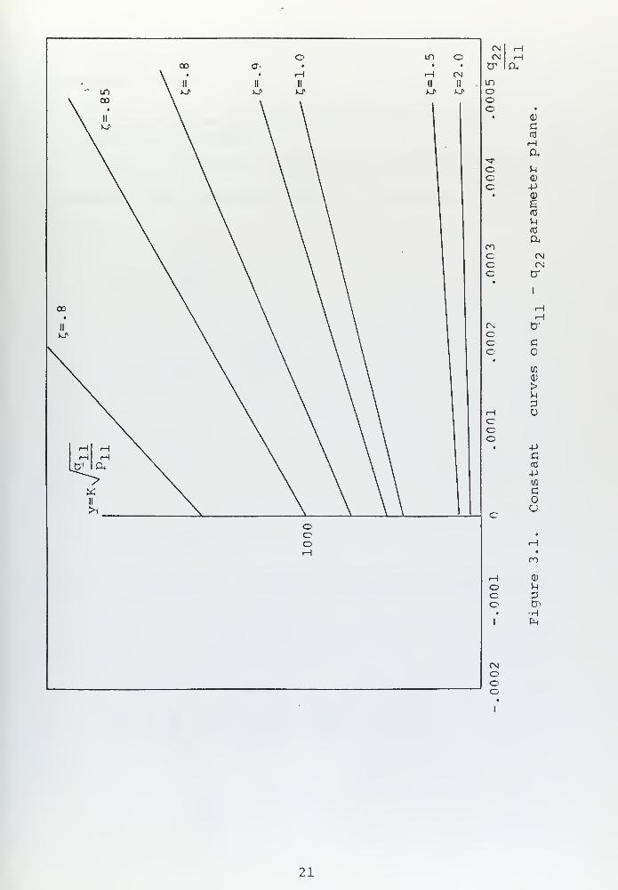
It can be noted that the constant C curves are straight

lines , but the location of the family for < £ < 1 depends

on K and p , i.e., the effect of q., , and q„_ can be showno o ^11 ^22

only for a specific plant.

Figure 3.1 shows the parameter plane for the plant with

K = 1600, p = 30.o ' *o

From section B the cost function for the optimal system

was :

'11 K11

'11L

2 2^22 /^ll^o o p n n o v p-o pn 11

x2(0)

+ f N/^7 xl(

0)x2(0)

o ^11

K'

-p +^O p + K

^o o p

q 22(-^=0 ± 2K

11

110V p11

x2

(0)

Let

Jl

=

P11[x

1(0)]

q ll \ / 2 2 g 22 q llop,, * o o 'p,,' o p 11

= yVp 2+ K

2x ± 2yo

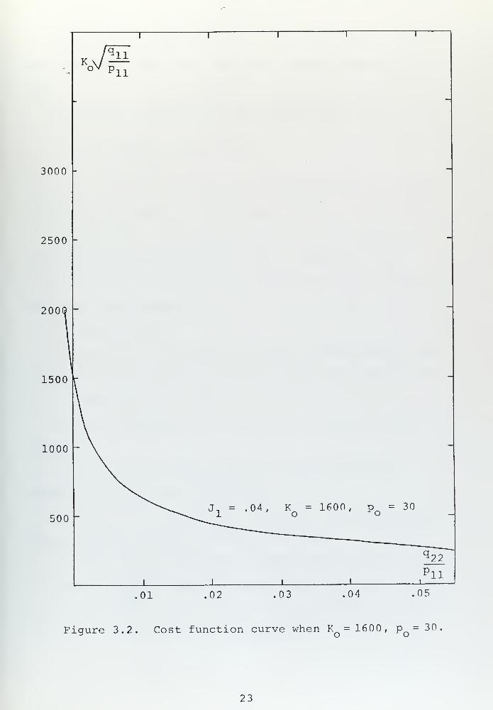
For the optimal system:

J, = .04, K = 1600, p = 301 o *o

20

CN rHCN iH

O1 aLDOOc •

• <u

cCO

rH

a"Stf

c ^c (D

c 4->

• CD

£<c

^fd

amc CNc CNi

c cr

exccc

cco

tr

c

>upu

4-1

c

4-)

CO

Co

ro

H CD

O uC 3o CT>

• •H1 fc

CMOOO

21

q22A constant cost curve is shown in Figure 3.2 in the vs

2Pl1

to parameter plane.

C. EFFECT ON DAMPING AND COST, STEADY STATE ACCURACYAND SPEED OF RESPONSE

In order to study the effect of the weighting factors

on damping in the parameter plane it is necessary to use

1 . 2 and 1.3.

VPll

let

2 q 22K -^-

q22= Wq

xl

then

X.= | v/^- + Wz ± 2 (3.1)

From this equation the following expression can be obtained:

p2 = -z(±2 - 4C

2) -Wz 2

(3.2)

As K is defined in Section A as:

K2 = -i^yp 2 -2 g*w;^

where

P ll

22

3000

2500 -

2000 "

1500

1000 -

500 ~

Ficrure 3.2. Cost function curve when K =1600, p =30.o

23

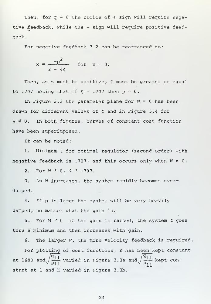
Then, for q = the choice of + sign will require nega-

tive feedback, while the - sign will require positive feed-

back .

For negative feedback 3.2 can be rearranged to:

2

x = —^ for W = 0.

2 - 4C

Then, as z must be positive, C must be greater or equal

to .707 noting that if C = .707 then p = 0.

In Figure 3.3 the parameter plane for W = has been

drawn for different values of £ and in Figure 3.4 for

W ^ 0. In both figures, curves of constant cost function

have been superimposed.

It can be noted:

1. Minimum C for optimal regulator (second order) with

negative feedback is .707, and this occurs only when W = 0.

2. For W > 0, C > .707.

3. As W increases, the system rapidly becomes over-

damped.

4. If p is large the system will be very heavily

damped, no matter what the gain is.

5. For W > if the gain is raised, the system C goes

thru a minimum and then increases with gain.

6. The larger W, the more velocity feedback is required

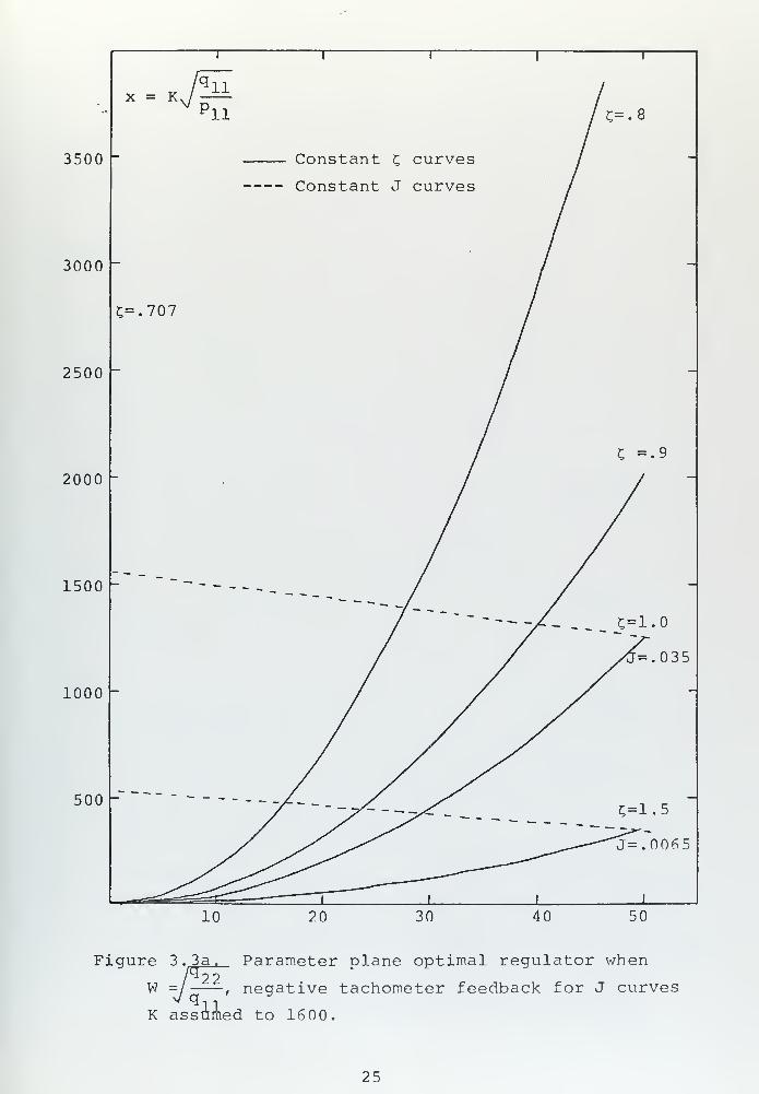
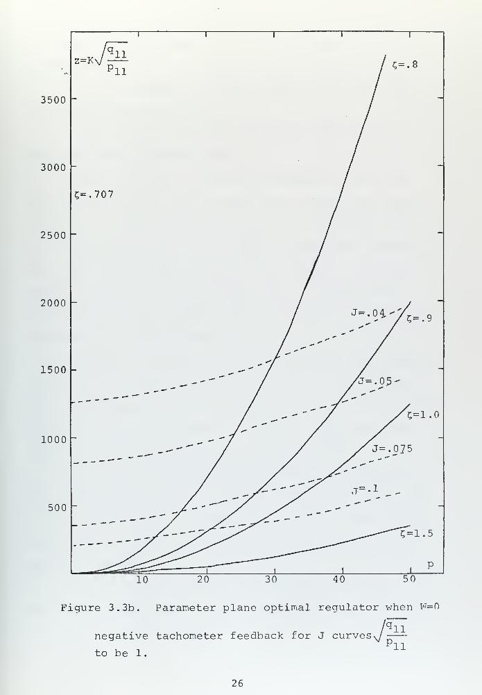
For plotting of cost functions , K has been kept constant

/^ll F*llat 1600 and./ varied in Figure 3.3a and / kept con-V P11

y v/Pll

stant at 1 and K varied in Figure 3.3b.

24

x = K,

l 1 I 1 l

ll11

^ Pll /c=.8

3500 Constant £ curves /

— —-- Constant J curves /

3000

C=.707

/

2500

/ ? =.9

2000

1500 - ~ --______

/ / yrf=.035

1000

500 - -

^S ^^ ^^-^^"j=. 006 5

i

""*i i I

10 20 30 40 50

Figure 3

.

3 a

.

Parameter plane optimal regulator when22

, negative tachometer feedback for J curvesW =j

K assumed to 1600.

25

I 1 1 i 1

'.,.

v /qi1 /z=Kv / r_ o

Pll /C_ ' 8

3500

/ "

3000 /C=.707 /

2500 /

2000 // j=.0i*V_

*v" /1500

---"*"" / yj=.o5-

/'''""/ y^5" 1 '

1000~~-—-"/ / A^500'---^0^^-

-<^=^——^^T^ , .

p

10 20 30 40 50

Figure 3.3b. Parameter plane optimal regulator when W=0

negative tachometer feedback for J curves'

to be 1

.

11'11

26

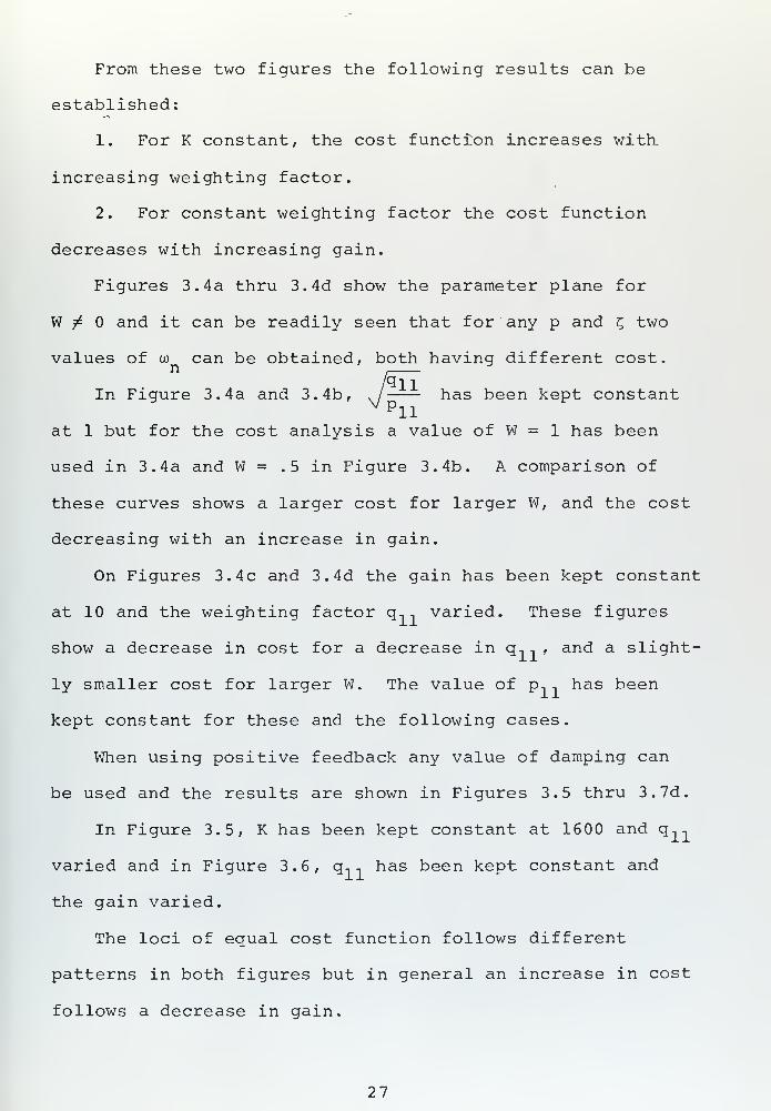
From these two figures the following results can be

established:

1. For K constant, the cost function increases with.

increasing weighting factor.

2. For constant weighting factor the cost function

decreases with increasing gain.

Figures 3.4a thru 3.4d show the parameter plane for

W ^ and it can be readily seen that for any p and z, two

values of co can be obtained, both having different cost.n

imiIn Figure 3.4a and 3.4b, ./ has been kept constantpll

at 1 but for the cost analysis a value of W = 1 has been

used in 3.4a and W = .5 in Figure 3.4b. A comparison of

these curves shows a larger cost for larger W, and the cost

decreasing with an increase in gain.

On Figures 3.4c and 3.4d the gain has been kept constant

at 10 and the weighting factor q, , varied. These figures

show a decrease in cost for a decrease in q,,, and a slight-

ly smaller cost for larger W. The value of p, , has been

kept constant for these and the following cases.

When using positive feedback any value of damping can

be used and the results are shown in Figures 3.5 thru 3.7d.

In Figure 3.5, K has been kept constant at 1600 and q,,

varied and in Figure 3.6, q, , has been kept constant and

the gain varied.

The loci of equal cost function follows different

patterns in both figures but in general an increase in cost

follows a decrease in gain.

27

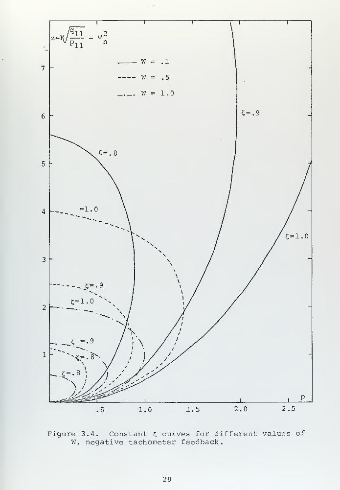
Figure 3.4. Constant £ curves for different values ofW, negative tachometer feedback.

28

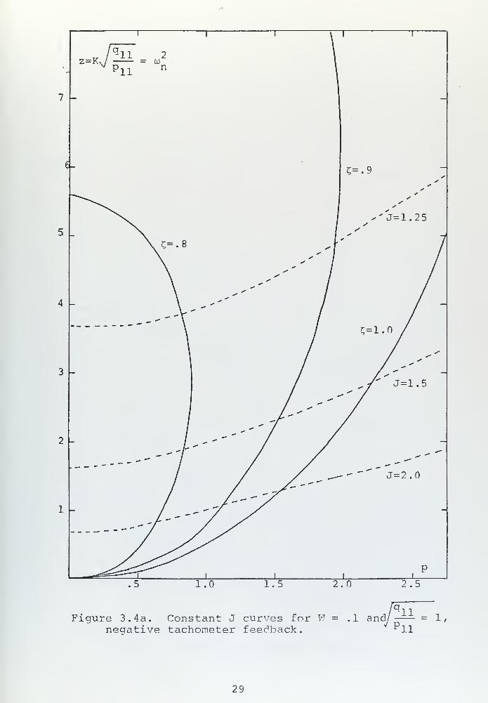
Figure 3.4a. Constant J curves for W = .1 and/negative tachometer feedback.

11

11= 1,

29

7 _

6 _

5 _

3 _

2 _

1 _

1 1 i i i

* /qH 2

z=K J = oj

^11

-

J=1.0s

ss

ys

ss

*s

••

s _ss«»

**•

»»*»

«*^-^

***•

**^^-

^*\t=i.o^v „J=1.25

X. •x ^»

\ •\ ^\ /\ ^\ ^\ .«»

—--^ =* 9 -*'\

**

—

v>^ •""'

^V. _ - *" ^-J=1.5^w *^ -^ ^

— •» "" ^S. _

•— — "" ~" " "N.

^-

\ ^*~"

\ -"f

- V'"" /

T^r""" j /)//

—^^^^\ i i i i

P

.5 1.0 1.5 2.0 2.5

Figure 3.4b. Constant cost curves for W = .5 and

fillv/pu

= 1, negative tachometer feedback.

30

v / 1:L 2z=KJ =00

'11W=.l

W=l

J curves J=.9

\

\

I

/

I

I

I

/

/

/

/

/j=L0

/ /

/ /

J=0.02

2.5

Figure 3.4c. Constant J curves for W = 1.0 and K = 10

,

negative tachometer feedback.

31

1.0 1.5 2.0 2.5

Figure 3.4d. Constant J curves for W =

negative tachometer feedback..1 and K = 10,

32

1400 -

1200 -

1000 -

800 -

600 -

400 -

200 ~

Figure 3.5. Constant C curves for W = and positivefeedback for constant J curves, K = 1600.

33

1400 "

1200 ~

1000

800 ~

600 ~

400

200

ELgure 3.6. Constant curves for W = and positivetachometer feedback for constant J curves

,

J.

q21 i.

34

A comparison between Figure 3.3 and Figure 3.5 shows

that for negative feedback values of ? >_ .707 are restricted

to the first quadrant while for positive feedback any value

of C is permissible.

Figures 3.7 show the parameter plane for two different

values of W and for different c.

A comparison between negative and positive feedback

shows same results as for W = 0, i.e., any value of £ is

permissible in the first quadrant for positive feedback.

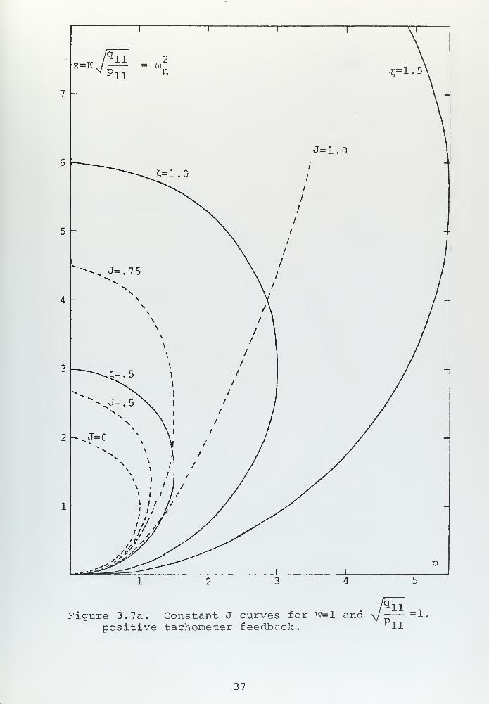
Figure 3.7a and 3.7b compare the effect on cost of

different values of W, keeping q, , constant and varying the

gain which results in larger cost, which for p = 1.5 is

0.75 for W = 1 and 1.25 for W = 2.

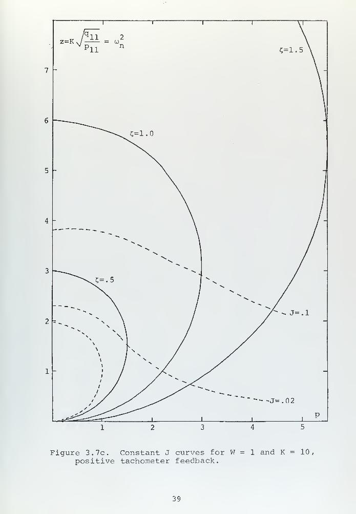
Figures 3.7c and 3 . 7d compare effect on cost of dif-

ferent values of W, keeping the gain constant at 10 and

varying q, , . For a small value of p the cost is smaller

for W = 1 than for W = 2 and for any u) there is a minimum

cost, which for w = .7 is about 0.19 for W = 1 and 0.3n

for W = 2.

Keeping K = 1.0 and K constant at 10 , a curve of cost

against frequency has been drawn and the results shown in

Figure 3.8. It can be seen that the cost follows the shape

of a parabola increasing very fast as the frequency

approaches 2

.

In order to study the effect of the weighting factors

on the steady state accuracy it is convenient to refer to

the equivalent block diagram of Chapter I. It can be seen

that

35

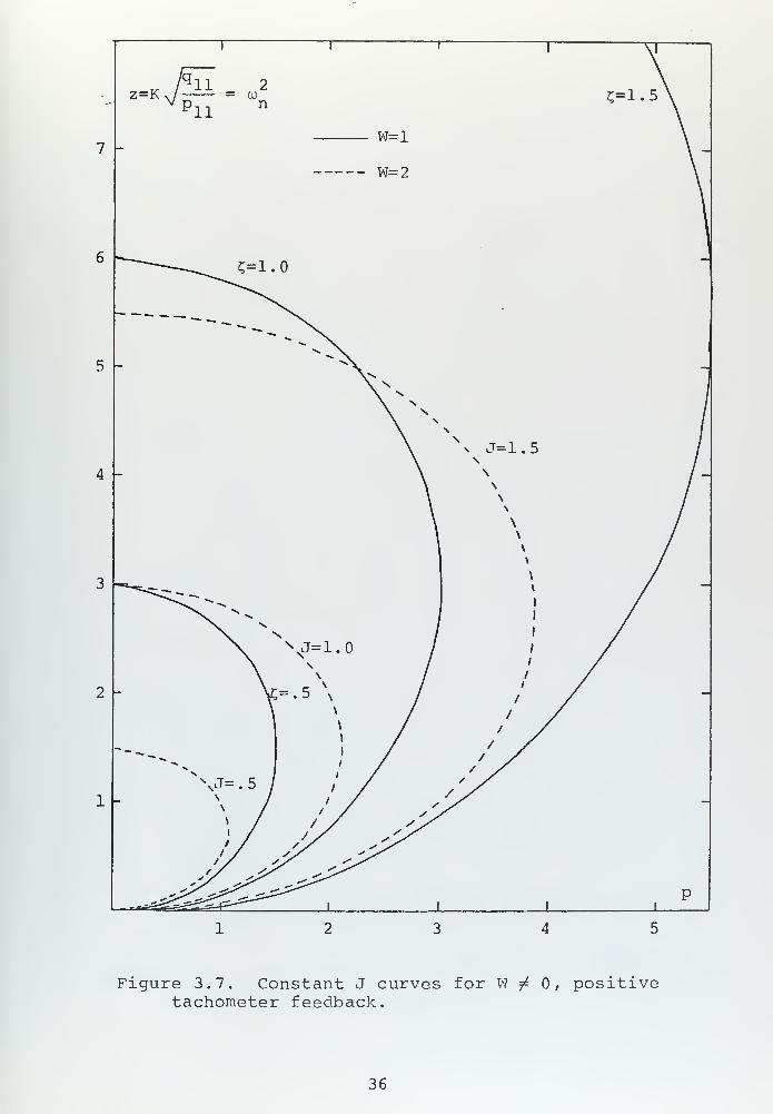
Figure 3.7. Constant J curves for W ^ 0, positivetachometer feedback.

36

1 ii VI

v /qH 2

z=K./ = w£=1.5>^PU

7

J= l . n

6' ^-^£=1.0 /

/

/

/

v /\ /

5

"^-^ J=.75

S

\ /

\ /

\ /

\ /

\ /

\ /

4\\

\\

\

A/ \

/ \

/ 1

\

\/

3 \

^~-\^=. 5 \

/

/-

*H ^v 1 /"**• \ 'N NJ-.5\ '

/ /

N \ 1 tiV \ '

\ \ 1/ /

\ \, / 1 j

2^=0 x

\ X

^ x

/]

\ 1 / //

/

/

/

1 1 / / //

11/

J

i ii

P

Figure 3.7a. Constant J curves for W=l andpositive tachometer feedback.

11'11

= 1,

37

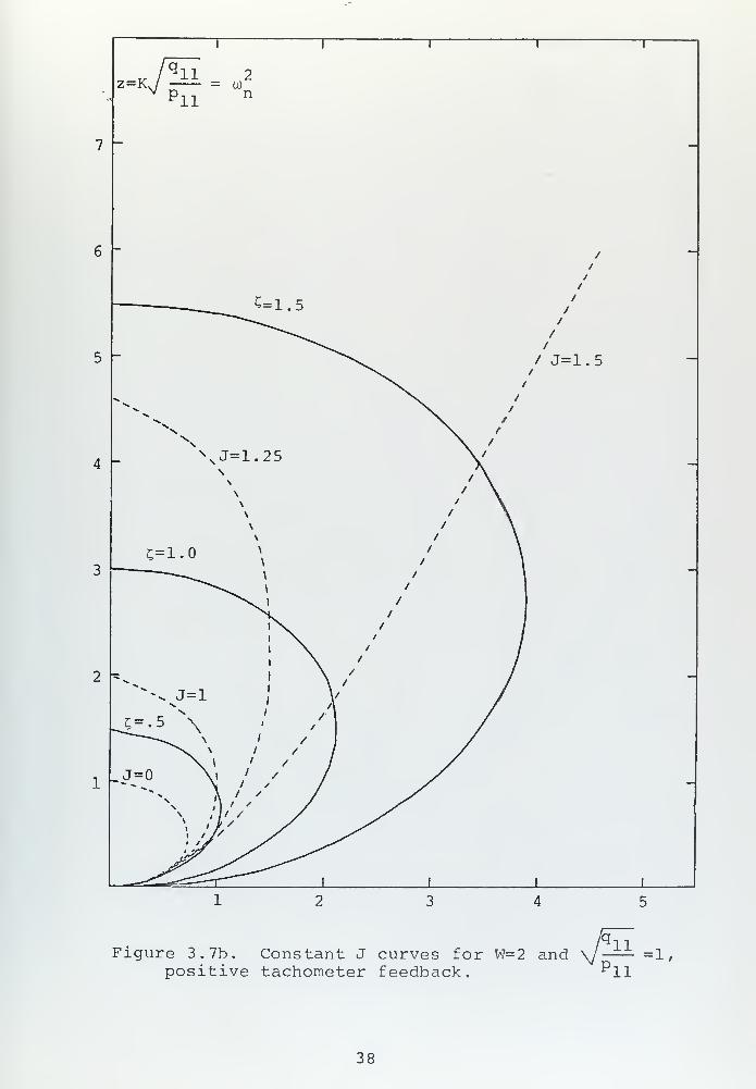
Figure 3.7b. Constant J curves for W=2 andpositive tachometer feedback.

11'11

=1,

38

1 i 1 1 \l

* /qH 2z=K v / = oj \Vpn n c=i.s\

7 V

6\

"""^^C-l.O

5 \

4

__ \ /

^N. \ /**» \ /X 1 /

>» /s

V. s>.

3 /^\£=.5 ^ /

^\. "** />^ / ^* /X / "** /\ / ^ /\ / """ /"*-

~. \ / >.j=.i2

K \ / /****"* S \ / /

x ^ \ / /V \ / /\ \ I / /

\ \ / /N N / /\ / s / /» / N / Sv

/ > / v'

1» / x^ *•» V^i / X *" >^

/ / """• ^^/ / yT >^~

/ / >^ S^ *"* -. ___

/ ^T ^X ^^^ *"" «. ^'/ ^/ ^^ "---J=.02/ / -x^ ^*^

'y ^^ ^~-—X^^ -*^ ^-^^ _^>^-<^^-^^ 1 1 p

. -^*<Lr <~—f" 1 1 1 1

Figure 3.7c. Constant J curves for W = 1 and K = 10

,

positive tachometer feedback.

39

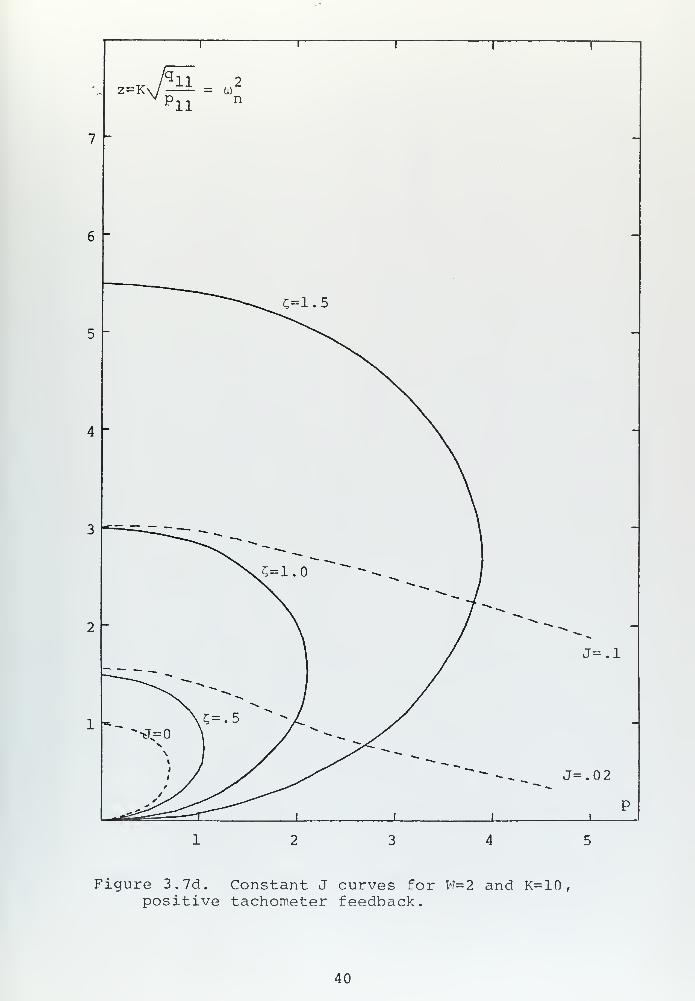
Figure 3.7d. Constant J curves for V7=2 and K=10,positive tachometer feedback.

40

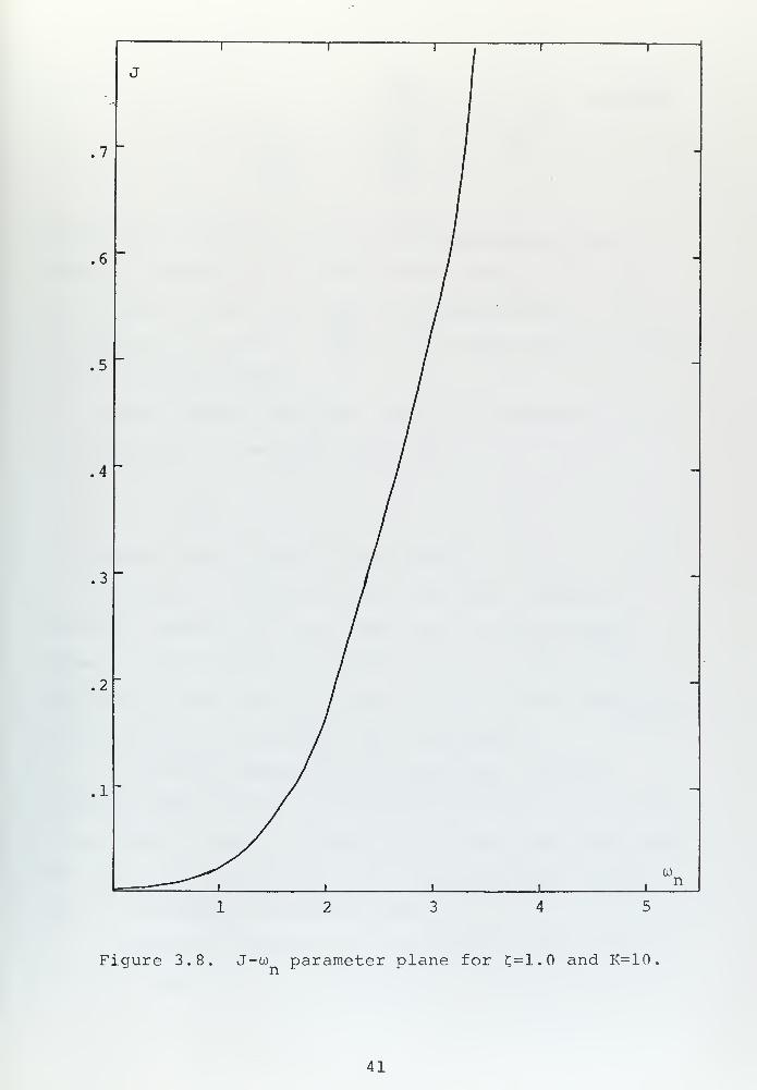
Figure 3. J-oo parameter plane for £=1.0 and K=10.

41

E

hipn I

SS , 1 I z . ,

111 v/ " + 1

11'11

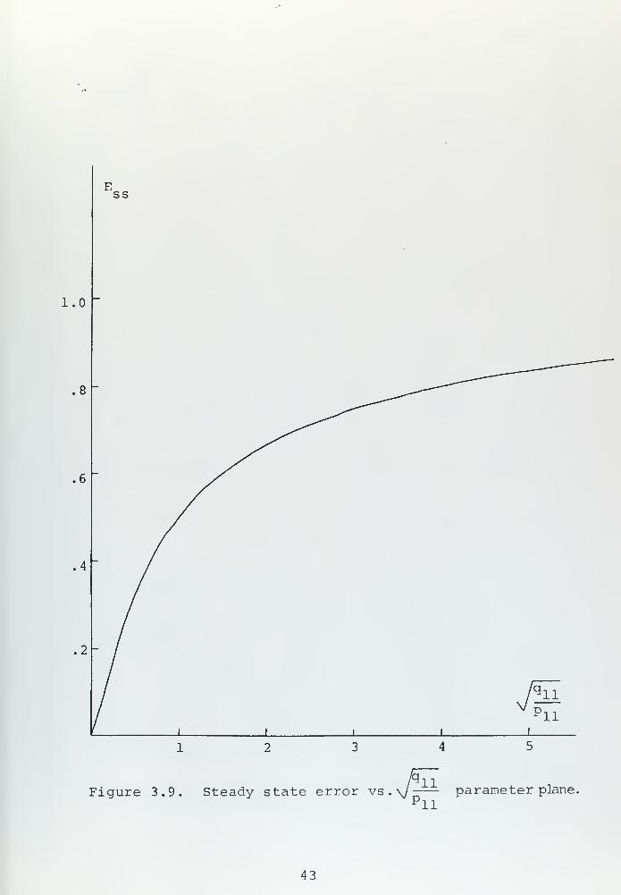
which will depend only on q-Q and the parameter plane is

shown in Figure 3.9. For small values of q, , the steady

state error is also very small, increasing rapidly as q,

,

ft!increases to a value of w = 2, and then slowly approach-pll

ing 1.0 in the infinite.

For the speed of response study it is convenient to use

the definition of settling time, i.e.,

Ceon

Several cases should be considered:

1. Negative feedback for the velocity. Curves of

constant settling time have been drawn in the parameter

plane for two different weighting functions, W=0 and W=2,

the results being shown on Figure 3.9a. It can be seen that

the settling time decreases with increasing W.

2. Positive feedback for the velocity. Constant

settling time curves for the same parameters as in the pre-

vious case are shown on Figure 3.9b. This curves show that

the settling time decreases with increasing W but faster

than in the negative feedback case.

3. Negative feedback for the position. The results

are as in Case 1.

42

Ess

1.0-

.8

.6 /

.4

.2 - /

Mi'

I li i i

Figure 3.9. Steady state error vs.\y-— parameter plane11

11

43

*\^^ l I 1 1 i

^iiX-•- z=K/- \ W=07p

ll \7

\ W=l ~

6

\ T = 2

-

5

\

4 \ -

3

-*» \\ \

\ \v \\ \

N \

s \

-

2\ \

^-^^ \ \^\T = 4 \ \

^\ \ \

\. \ \~--> T = 4 \ N \

1

N \ \\

\\ i

i \ i \ .

p

Figure 3.9a. Constant settling time curves for negativetachometer feedback.

44

1 I 1 1 I

v /qH 2. a=K>/ = u T7 rtv p, , n W=0

W=l i

7

6/ T== 4

/ -

5 ~~"^^T= 2 /

v. /

N /N / / T = 2N /

S /

S. /

X /N /

4 — X /

N /\ /\ /

1 \

3 ^^ /N

"s T-4 / \N / \

/ *

/2 \ / V

V / »

/ '/l

/ l /1

1 / /; / /

// /if I

i / i I

Pi

Figure 3.9b. Constant settling time curves for posi'

tive tachometer feedback.

45

4. Positive feedback for the position. Using Routh

criteria of stability it can be seen that this case gives

a pole in the right hand plane, meaning that the system will

be unstable and the regulator will not regulate at all.

46

IV. SENSITIVITY IN THE OPTIMAL REGULATOR

A. GENERAL

An optimal design guarantees minimum cost for the regu-

lator from any initial conditions.

If any parameter of the regulator deviates from the

value used in (or determined by) the optimal design, then

the cost of regulating is increased, i.e., the performance

of the system is not optimal.

Sensitivity is a word used to describe the rate at

which some characteristics of the system deviates from a

reference value as a function of a parameter change. Thus

various types of sensitivity could be defined:

a. Root sensitivity

b. Bandwidth sensitivity

c. Steady state accuracy sensitivity

d. Settling time sensitivity

e. Rise time sensitivity

f. State sensitivity

g. Cost sensitivity

State sensitivity is a measure of the deviation of a

dynamic state from the values it would assume if the system

was optimal.

Cost sensitivity is some measure of the deviation of

the cost from the optimal cost.

Ultimately all of these various sensitivities relate to

the same basic characteristics of a linear regulator, i.e.,

47

they indicate changes in root location (possibly excepting

steady state accuracy sensitivity) . However there must be

some basic differences in these various sensitivities in

the sense that some are vector quantities and others are

scalars , i.e., root, bandwidth, settling time and rise time

sensitivities all indicate pretty clearly the direction in

which a root has moved, while cost sensitivity only indi-

cates the magnitude of the root motion.

From a design point of view there may be some advan-

tages to the cost sensitivity, i.e., one can usually accept

dominant root location within a specified s-plane area,

and a defined area on the parameter plane normally maps

into a dominant area on the s-plane. Correlation with

other performance criteria may very well be required.

Cost may be evaluated at any point on the parameter

plane and thus constant cost contours can be obtained.

Cost sensitivity in a macroscopic sense is then just the

difference between two costs divided by the increment in

parameter value between them.

Cost sensitivity can also be evaluated at a point and

normally the point of greatest interest on the parameter

plane would be the point at which the parameter assume

optimal values. Change in cost from this optimal value

(for a small change) can be computed by:

Tx Aparameter = AJ

d (parameter)

J4_

+ AJ = J 4.opt at new point

48

This however depends on initial conditions values,

and the permissible range of A parameter depends on the

system and on the cost function.

B. SENSITIVITY OF THE COST FUNCTION AND SENSITIVITYOF THE OPTIMAL COST FUNCTION

In the research, the curves of constant J on the parame-

ter plane are obtained using an expression for J which is

derived in terms of p, K, K, , K_ , where p and K are plant

parameters and K, and K_ are values for the state feed-

back loops. In order to use the expressions the system is

optimized at some chosen p and K, and values of K, and K~

are computed for the system thus optimized. When J is set

to a non-optimal value K, and K_ remain fixed at the opti-

mal values and p and K are computed. The system is not

optimal for the new p and K.

Sensitivity of the optimal system could be defined by

taking the derivative of the cost function, i.e.,

sJ =

9Jo

op3P P=Po' K=K

o

SJ =oK

Jo

9KP=Po' K=K

o

However the equation for J optimal can be written in

at least two forms

:

A. The form is used to compute J curves, which con-

tains the feedback gains K, and K_ as constants.

B. A form obtained directly from the R matrix such that

K. and K do not appear as symbols, the cost being

49

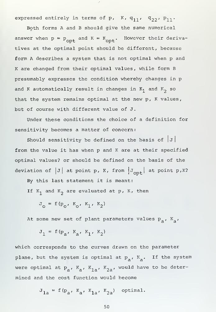
expressed entirely in terms of p, K, q,, , ^22' ^11"

Both forms A and B should give the same numerical

answer when p = p and K = K \_. However their deriva-c ^opt opt

tives at the optimal point should be different, because

form A describes a system that is not optimal when p and

K are changed from their optimal values, while form B

presumably expresses the condition whereby changes in p

and K automatically result in changes in K-. and K~ so

that the system remains optimal at the new p, K values,

but of course with different value of J.

Under these conditions the choice of a definition for

sensitivity becomes a matter of concern:

Should sensitivity be defined on the basis of | J|

from the value it has when p and K are at their specified

optimal values? or should be defined on the basis of the

deviation of J] at point p, K, from JJat point p,K?

By this last statement it is meant:

If K, and K~ are evaluated at p , K, then

Jo

f(Po' V Kl' V

At some new set of plant parameters values p , K ,a a

Jl = f(Pa' V V K 2>

which corresponds to the curves drawn on the parameter

plane, but the system is optimal at p , K . If the systema a

were optimal at p , K , K, , K„ , would have to be deter-a a la z ex

mined and the cost function would become

Jla

= f(Pa' V Kla'

K2a> °Ptimal «

50

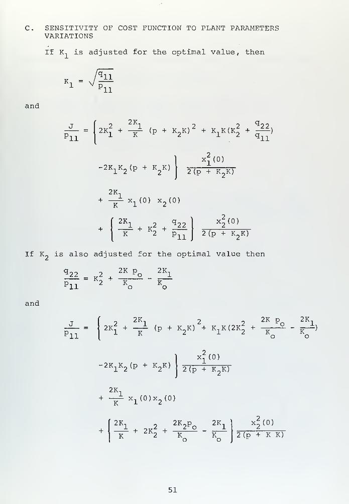
C. SENSITIVITY OF COST FUNCTION TO PLANT PARAMETERSVARIATIONS

If K, is adjusted for the optimal value, then

1 V p

11

11

and

'11

22K

12K

1+ IT (P + K

2K) + K

1K(K

2+q^>

-2K1K2(p + K

2K)

2K n

x2(0)

2(p + K2K)

+

+

— xl(

0) x2(0)

2K1 2 q 22

K 2 p11

x2(0)

2(p + K2K)

If K2

is also adjusted for the optimal value then

^22 72K Po 2K

1

Pll 2 Kc

K

and

'11

22K

12KT + -

1 K(p + K

2K) + K

1K(2K

2+

2K p;_<

K

2K.

-2K1K2(p + K

2K)

2K,

X2(0)

2(p + K2K)

— x1(0)x

2(0)

2K, 2K oP^ 2Ki

-r + 2K2

+ -^ - r2x2(0)

2 (p + K K)

51

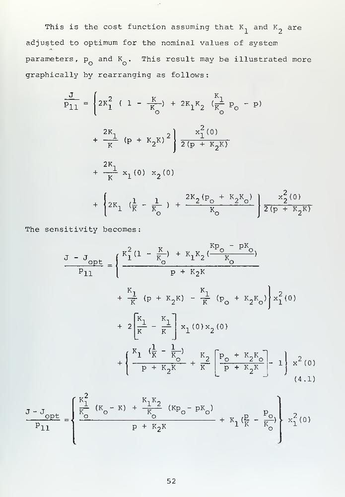
This is the cost function assuming that K, and K? are

adjusted to optimum for the nominal values of system

parameters, p and K . This result may be illustrated more

graphically by rearranging as follows

:

KK.

Pii = 2Ki ( 1 ~ -V-) + 2K

iK o (rT- P~ - P)'11 K 12 V K *o

o

2K.

K

2K.

(p + K2K)

x*(0)

2(p + K2K)

+ •— x, (0) x (0)

2KX (| - ^ ) + 2 ^o 2 o

K,

4(0)2(p + K

2K)

The sensitivity becomes

KP~ " PK

J - J2P_t = ,

'11

Kl(

l - —) + KlK 2(-

o o_

p + K 2 K

K K+ 4 (P + K

2K) - ^ (p + K

2Ko ) x^(0)

+ 2K K

x1(0)x

2(0)

1 *K K ; K.°_ + .J.

p + K K K

p + K K^o 2 o

p + K2K

- 1 x2(0)

(4.1)

J - J2P_t = <

'11

ir (Ko" K) +~ir- (kp -pk

o'o o

p + K2K

+ Ki<l-ir»o

> x*(0)

52

+ 2K.1 J_K ' K

x1(0)x

2(0)

+ <

K - KKl (-%~'

+K2 (pQ

- p) + K2(Ko-K)

p + K,K K (P+K2K)

)

x2(0)

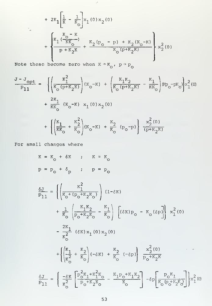
Note these become zero when K -»• K , p -> po' * ^o

J- Jopt _

'11

k:

\ (K -K) +K1K2

K.

(Kp -pK )

K (p+K K) I

l o ' K (p+K K) KK v *o *o' 1

\ ° 2J \

° 2 °l i

xf (0)

2K,—- (K -K) x, (0)x o (0)KK o 12K K

2

\K2

K*r+sr (VK) + k- (p -p»

o o / o

> 2X2(0)

(p+K2K)

For small changes where

K = K + 6Ko

K - K

p = p +6r ^o pP = P,

6J

'11

k:

K + (p +K-K )

, o ^o 2 o(1-6K)

i IKiK

:

K.

K p +K K Ko ^o 2 o o

2K.

(6K)pQ

- KQ (6p) x*(0)

K-f-

(6K)x1(0)x

2(0)

A\\^J\K.

,?+

K" PQ+K

2K

6J

'11

-6K

K2

rp2K n +K?K K,p +K,K "

*o 1 1 o l*o 1 2

p +K„K*o 2 o

K-6p

P K,^o 1

K (p +K.K )

O *o 2 ox*(0)

53

2K.

K2^ (6K)x

1(0)x

2(0)

+ <-K,+K K1 2 o

K.

IT (p +K K )o o 2 o

(6K) -K +(p +K K )o ^o 2 o

(6p) ^x^(O)

)

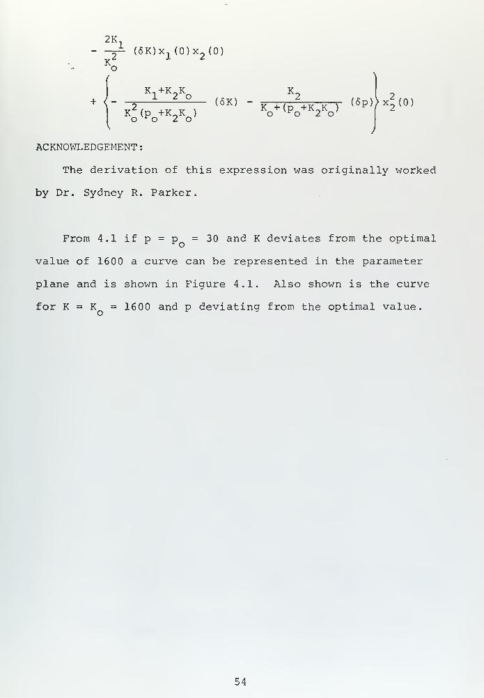
ACKNOWLEDGEMENT

:

The derivation of this expression was originally worked

by Dr. Sydney R. Parker.

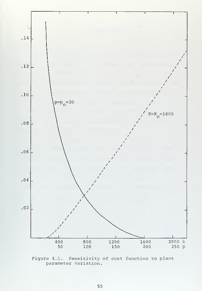
From 4.1 if p = p =30 and K deviates from the optimal

value of 1600 a curve can be represented in the parameter

plane and is shown in Figure 4.1. Also shown is the curve

for K = K =16 00 and p deviating from the optimal value.

54

„

i i i i 1

14

1 //

/

/1 /

12\ /1 /1 /

1 '

\ /

1 /

10 \ /

\p=p =30 /\ o /

\ / K=K =1600\ /

08

\ /

\ /

\ •

\ /\ /

06\ /

\ /

\ /\ /\ /

\ /

\ /

04\ /

\ /\ /

A./ \

/ \02 / \

/ \/ \

/ \/ X.

/ x./ x^

y i i i ^"^-^i i

400 800 1200 1600 2000 k

50 100 150 200 250 p

Figure 4.1. Sensitivity of cost function to plantparameter variation.

55

V. CONCLUSIONS

RESULTS

An optimal regulator can always be obtained using the

parameter plane method for any given plant. Both negative

and positive feedback can be used to achieve the desired

results but only negative position feedback should be used

to obtain a stable system. Positive position feedback

gives an unstable system with no regulation at all.

For a given plant an optimal cost function can be

obtained and the values of the feedback path gain calcu-

lated using the curves of Chapter II.

When a given frequency and damping is desired, the plant

parameters needed to achieve the results can be obtained

for different weighting functions with the use of figures

of Chapter III, or for a fixed plant the performance and

cost be obtained by the use of the same figures.

For plant parameters variations the sensitivity of the

cost can be obtained using the figure in Chapter IV.

35

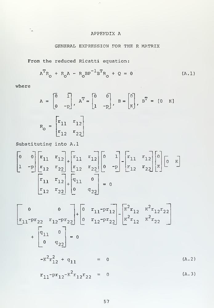
APPENDIX A

GENERAL EXPRESSION FOR THE R MATRIX

From the reduced Ricatti equation:

ATR + R A - R BP~ 1

BTR + Q =

o o o o(A.l)

where

A =1

-pAT = B =

ro

1 -p_i

_K_

B1 = [0 K]

R =o

rll

r12

r12

r22

Substituting into A.l

rll

r12

r r12 22

+rll

r12

r r12 22

1

-p

rll

r12

y r12 22

rll

r12

r12

r22

*11

q 22

=

K

rll

pr22

r12

pr22

+rn-pr

12

r12

-P r 22

11

22

=

2 2K r

12K r

12r22

2 2K r

12K r

22

„2 2-K r

12+ qn

11 ^12 12 22

=

rn-Prn"K r io r oo = °

(A. 2)

(A. 3)

57

rirPr12" K r12

r22

=°

2(r12

-pr22

)-K2r2 2+q 22

From A.

2

1112

K'

r = +12

L llK

(A. 4)

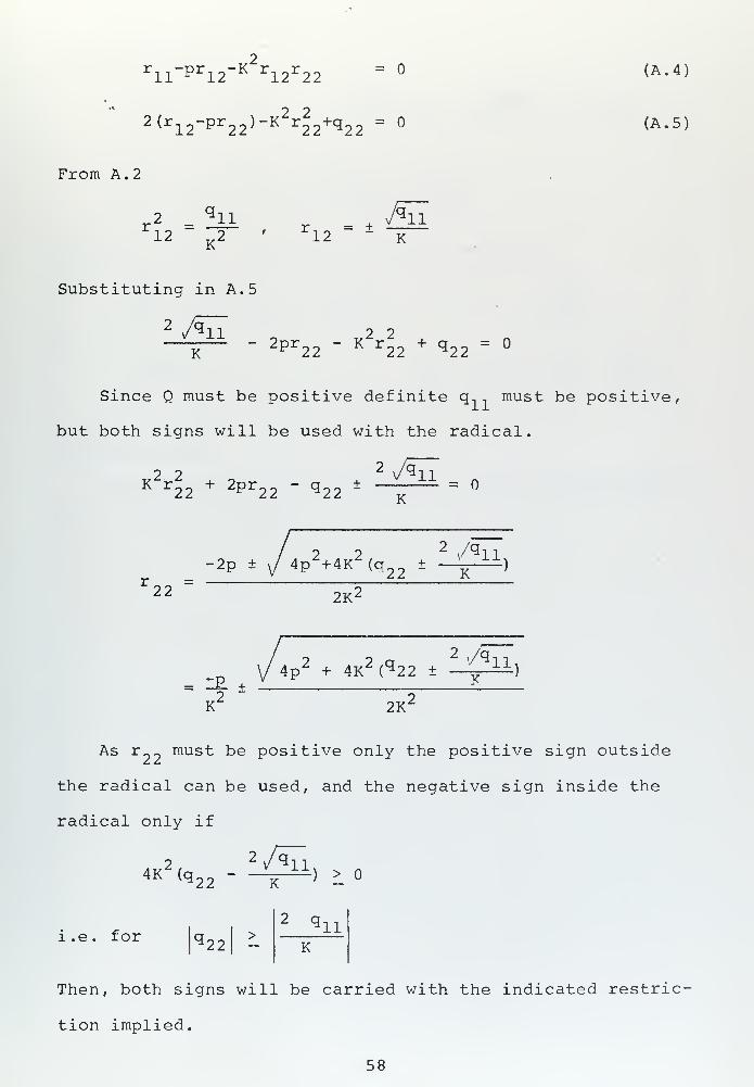
(A. 5)

Substituting in A.

5

2v/^IT .2 2

K' 2Pr 22 " K r

22+ q 22

=°

Since Q must be positive definite q, , must be positive,

but both signs will be used with the radical.

K2r2

2+ 2pr

22- q 22

2v/qll

± —-—— =K

-2p ± /4p 2+ 4K

2(q 22

±

2 /q 11.

K22 2K<

_ \/4p2

+ 4K2

(q 22 ± -~^)

K' 2K'

As r~~ must be positive only the positive sign outside

the radical can be used, and the negative sign inside the

radical only if

22 /qTl

4K (q 22 " "V^ ^°

i.e. for22

2 q 11K

Then, both signs will be carried with the indicated restric-

tion implied.

58

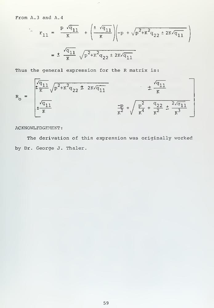
From A. 3 and A.

4

p yq. 1111 K

/qnV /ap +K q 22

± 2K/q^

. + ^11K p

z+K

zq 22

± 2K/q^

Thus the general expression for the R matrix is:

R =o

/q 11K yp

2+K

2q 22

± 2K/qxl

+ ^iTK

K ^ +2

E_ +4 2

K K

q 22 +2/^Tl

K"

ACKNOWLEDGEMENT

:

The derivation of this expression was originally worked

by Dr. George J. Thaler.

59

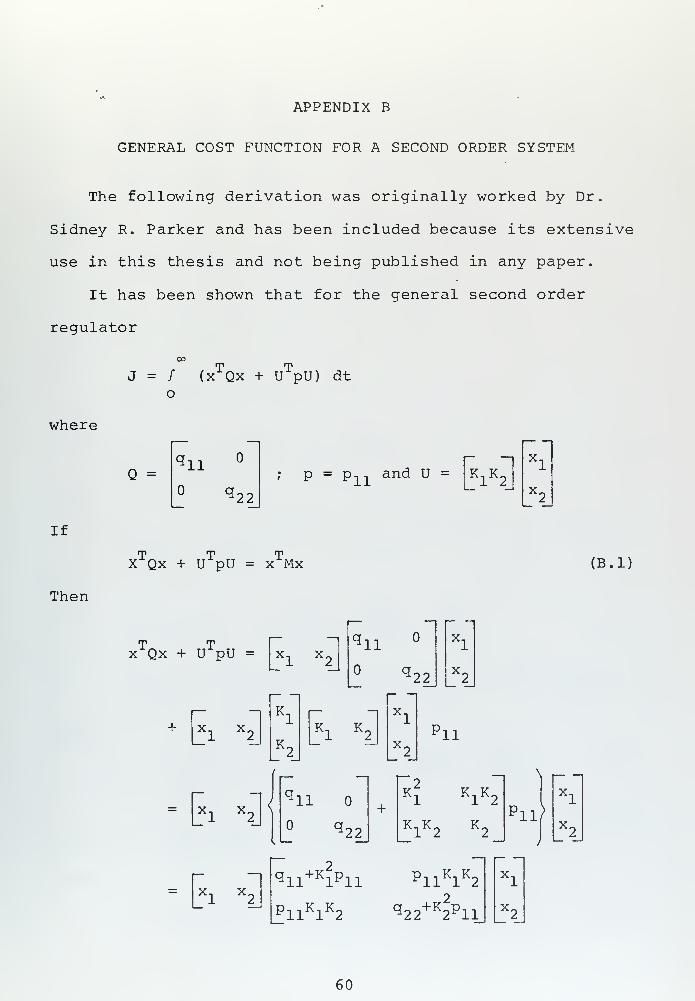
APPENDIX B

GENERAL COST FUNCTION FOR A SECOND ORDER SYSTEM

The following derivation was originally worked by Dr.

Sidney R. Parker and has been included because its extensive

use in this thesis and not being published in any paper.

It has been shown that for the general second order

regulator

J = / (xTQx + U

TpU) dt

where

If

Then

Q = «11

q22

/ P =P-i -i

an<3 U = K1K2

x.

T T TX Qx + U pU = x Mx (B.l)

— — —

T Tx Qx + U pU =

- —

x2

*11 (

q;

)

>2_

xl

_X2_

+ xx

x^Kl

K2_

Kx

K^xi

_

X2_

?11

Kl

K1K

*1K2K2

1 ^

= x1

x^q ll

_0 q^+

2b>

Xl

l_

X2_

=*1 x

2_Pi] k

ik

:2

LI I

q 2:

>11K1K2

2

2p ll

xi

X2

60

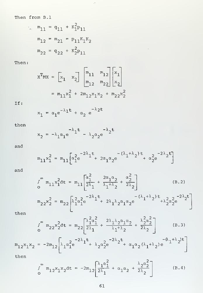
Then from B.l

-mll

= q ll+ K

lpll

m12

= m21

= P11K1K2

m22

= q 22+ K

2pnThen:

TX MX -h

mll

ml2

m12

m22

x.

X,

mll

xl

+ 2m12

x1x2

+ m22

x2

2

If:

-Xitx, = a, e x + a~ e

-X 2 t

then-x.t -x

2t

x2

= -X^e - X2a2e

and

m, , x, = m11"1 "11 1

-

7-2X t -(X +X )t

afe + 2a n a„e12 + a^e-2X f

and

then

/ m, , x, dt = m, ,

o

-2 2-ia 2a

ia o

a2

2X^+ X-iT^

+2X^

(B.2)

m22

x2

= m22

- 2" 2A

it -(X +X )t

2 2-2X

2tn

X a e + 2X.Xa.a-e +X a e

00 p/ m _x dt = m

22 2 22

rXlal

2AlX2ala2

X2

0t21

2X x 1+ x2

2X2 J

(B.3)

m12

XlX2

= " 2m12

then

r -atX.. a, e

2" 2X

2t -(X^X^t

+ X_a2e + a,a

2(X.+X

2)e

/ m12

x1x2dt = -2m

o

"Xlal

X2a2

_

+ a, a~ +2X 12 2X

(B.4)

61

And

J = B.2 + B.3 + B.4

= m11

a 2

1

L2A

1

2ala2 a

x 1+ x2

2\

- 2m12

rXlal W|W X

2a2

2X x 1+ x2

2X,

+ m22

rXlal

2A1A2a1a2

X2X2

-.

2X. x 1+ x2

2A2 J

(B.5)

To find A., and X» let:

*> s (s+a)

K.

K.

x.

Ro s +as+K]_G

K s

x.

Rs2

+ (a+K G)s + K;

,G

a) = /kTgn 1

62

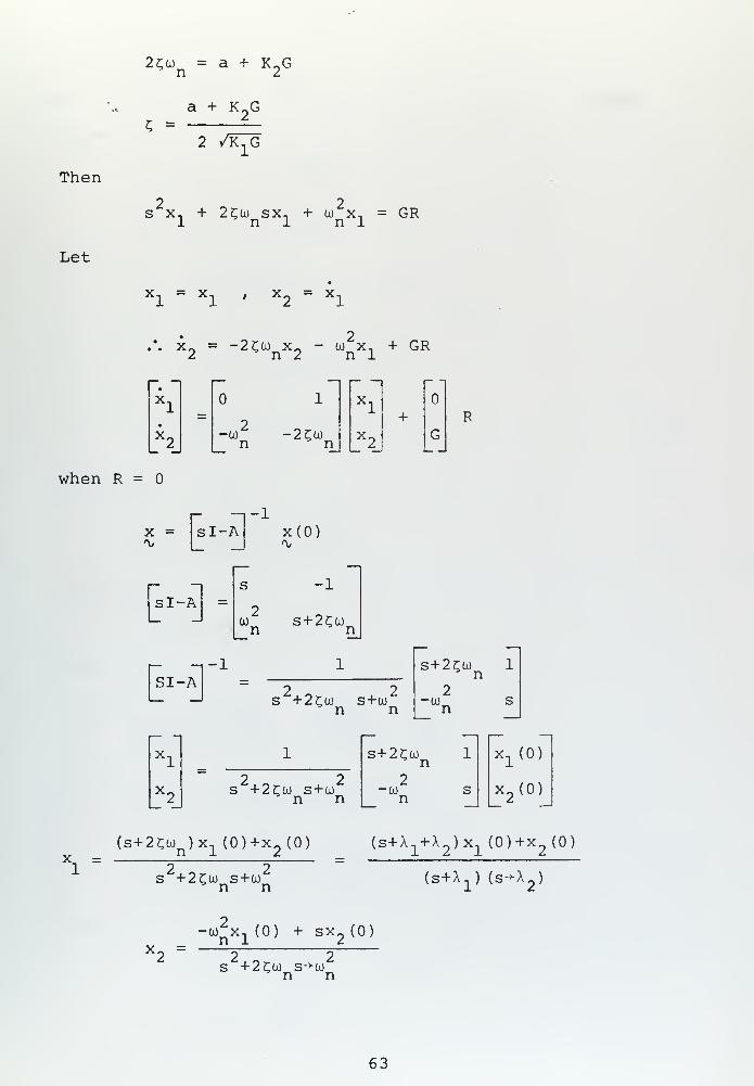
2£w = a + K~Gn 2

C =a + K

2G

2 /KjG

Then

Let

2 2s x, + 2c;co sx, + oo x, = GR

1 n 1 n 1

Xl

Xl '

X2

Xl

.*. x~ = -2£co x. - (i) x. + GR2 n 2 n 1

x.

x. -co -2Cojn n

r~ ~\

xl

+

_X2_

GR

when R =

x sI-A-1

x(0)

sI-A

SI-A

-1

oo s + 2c~;oon n

-1

2 2s + 2tco s+co

n n

s+2£oj 1n

-co sn

x.2 2

s + 2cco s+con n

s+2£oon

-con

x1(0)

x2(0)

x. =(s+2Cco

n)x

1(0)+x

2(0)

s +2Cw s+con n

(s+X1+A

2)x

1(0)+x

2(0)

(s+X1

) (s->X2

)

X2

=•oo^x, (0) + sx (0)n 1 z

2~Z 2s + 2tco s-*co

n n

63

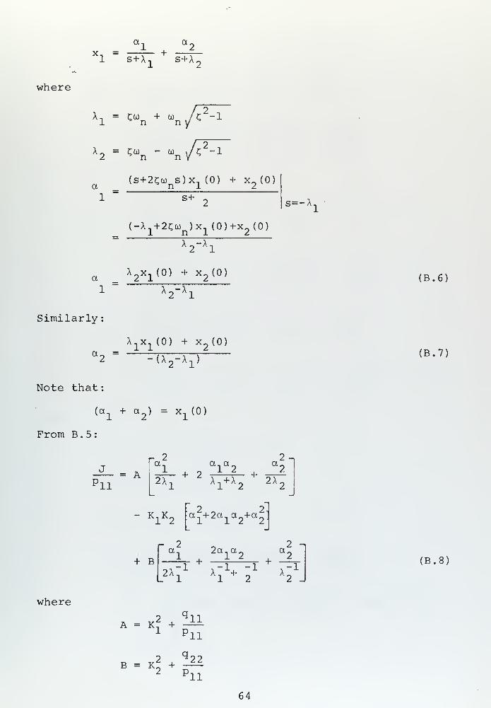
1 s+X, s+X.

where

1 n n "

X~ = £0) - CO </2 ^ n n V

c2-i

a(s+2cu s)x

n (0) + x (0)n 1 2

s+s=-X.

(-X.+2C0) ) x i(0)+x,(0)

x2-x

1

X2X1(0) + X

2(0)

i "x2-x

1

(B.6)

Similarly

:

a2

=X1x1(0) + x

2(0)

=Tx7^) (B.7)

Note that

:

(a1

+ a2

) = x1(0)

From B . 5

:

2 -,

'11A

Tan

a a a'

+ 2 : . +2X x 1+ x

22X

" K1K2

2 2-a +2a.

a

2+a

+ B

2 2-ia.. 2a-a_ a_

+ —, , +

L2A

1

XXi1+

2

1X-1

2 J

(B.8)

where

2 q lla = k: + -

i p li

q 22B = K~ + -

2 p11

64

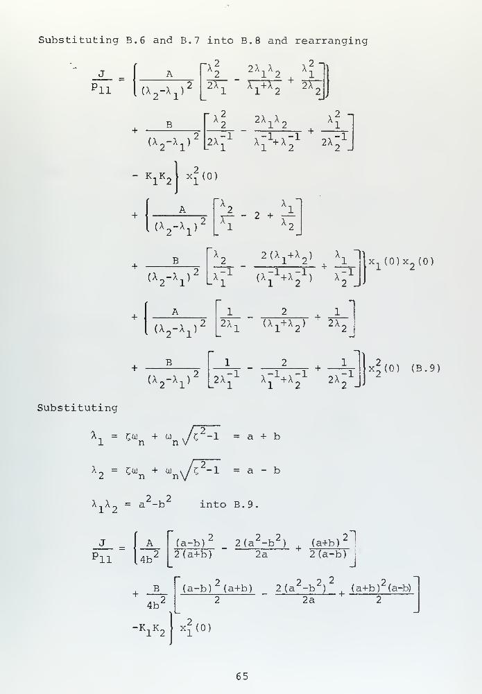
Substituting B.6 and B.7 into B.8 and rearranging

2 -v

'11

r~X 2A2

(x2-x

x )

2A1

T-^T2

2X1X2

+Xl

2X

+B

(X n-X n )

r 2 2-iX2

2X1X2

2 "1' L~"l2X,

1 X.Vx"" 1

1 22X

-12 J

" K1K2

\x*(0)

A

1<VV2 - ? 4- 1

i— * + ^

—

x1

x2

+B

<V*1>

X

^i1

2(X1+X

2) X

x

(X-^x" 1) X"^

x1(0)x

2(0)

+

(X^) 2A

2+ !

(A 1+ A2

) 2A2

B

(Xj-Xj)L2A

1 a-^a; 1+

2X-12 -M

x2(0) (B.9)

Substituting

A. = £> + 03 ./C -1 = a + b1 n n V/

X = £to +o) v /C -1 = a - b2 n nv

X,X_ = a -b into B.9.

'11

A

4b'

(a-b)'2 (a+b)

2~]2 (a -b )_ (a+b)

2a 2 (a-b)J

4b

"K1K2

(a-b)2(a+b) 2 (a

2-b

2)

|

(a+b)2(a-b)

2a

x2(0)

65

+4b'

A

4b:

B

a-b __ a+ba+b a-b

x1(0)x

2(0)

2+ 1

4b'

2 (a+b) 2a 2 (a-b)

a+b 2 (a2-b

2) a-b"]

2 2a 2J

x2(0) (B.10)

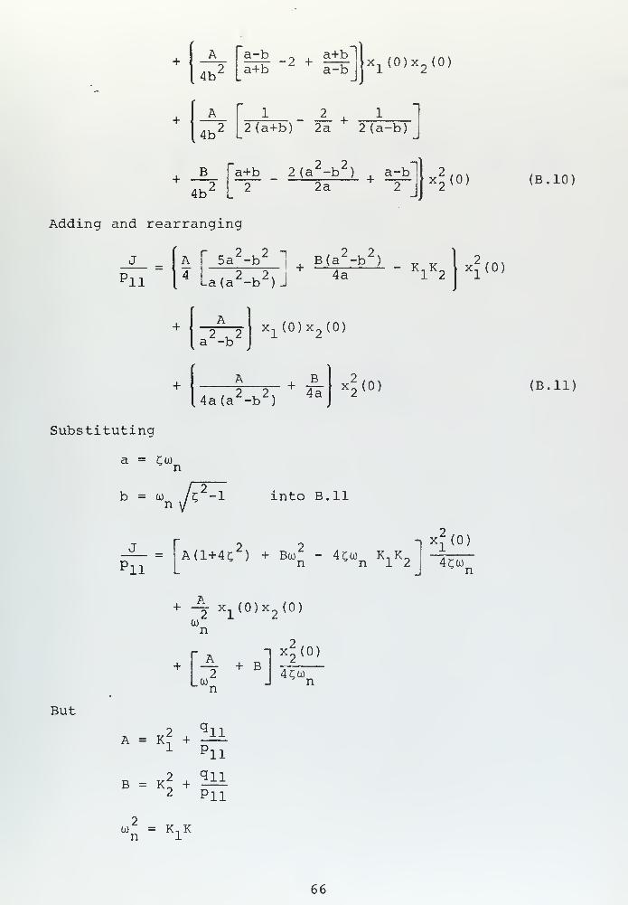
Adding and rearranging

f 5a2-b

2

'11

Aua(a2-b

2)

J

| +B(a

2-b

2) .

4a 12 » x2(0)

+

x]L

(0)x2(0)

2 2I4a(a -k> )

B4a

x2(0) (B.ll)

Substituting

a = Cojn

b - «n ./r into B.ll

'11

2 2 1X1(0)

A(1+4? ) + B% - 4C% KXK2

-jgj.n

But

+ -A.X;L (0)x 2

(0)

COn

[;7 + B

n

x2(0)

4Twn

A = K7 + -1 P

11

11

B = K2

+ 5112 Pn

OJ = K, Kn 1

66

Then '.,

2Cw = p+K„Kn ^2

'11

M ll2 2

q , (K,+ p,,) (p+K9K)

|- q

K7 + -ii + ± i±- = +K.K IC+ -^Pn |

KXK 1 \ 2 p'11 111

- 2K1K2(p+K

2K)

X^(0)

2(p+K2K)

2 q ll1 Pn

+ -K-K— x1(0)x

2(0)

2. q llk;+ -i p11

+ KI+.q 22

2 P11

*2 (0 >

2(p+K2K)

(B.12)

67

LIST OF REFERENCES

1. Athans , M. and Falb, P.L., Optimal Control , Chapter 9,McGraw-Hill, 1966.

2. Tuel, W. G., An Improved Algorithm for the Solutionof Discrete Regulations Problems , IEEE Transactionson Automatic Control , Oct. 1967.

3. O'Donnell, John J., Asymptotic Solution of the MatrixRiccati Equation of Optimal Control, Fourth AnnualAllerton Conference on Circuit and System TheoryProceedings , 1966.

4. Sinha, N.K. and Atluri , Satya Ratnam, Sensitivityof Optimal Control Systems , Fourth Annual AllertonConference of Optimal Control and System TheoryProceedings , 19 6 6.

5. Hsu, Jay C. and Meyer, Andrew U., Modern ControlPrinciples and Applications

,

McGraw-Hill, 1968.

68

INITIAL DISTRIBUTION LIST

No. Copies

1. Defense Documentation Center 2

Cameron StationAlexandria, Virginia 22314

2. Library, Code 0212 2

Naval Postgraduate SchoolMonterey, California 93940

3. Professor G.J. Thaler 3

Department of Electrical EngineeringNaval Postgraduate SchoolMonterey, California 93940

4. Professor S. R. Parker 3

Department of Electrical EngineeringNaval Postgraduate SchoolMonterey, California 93940

5. Lt. Lionel Doren 1

Av. Pedro de Valdivia 1828 Depto 101Santiago, Chile

6. Director de Armamentos de la Armada 1

Correo NavalValparaiso, Chile

7. Director de Instruccion de la Armada 1

Correo NavalValparaiso, Chile

69

UNCLASSIFIEDSecurity Classification

DOCUMENT CONTROL DATA -R&D, Security classification of title, bodv of abstrac t and indexing annotation must be entered when the overall report i s classified)

Originating activity ( Corporate author)

Naval Postgraduate SchoolMonterey ,- California 93940

Za. REPORT SECURITY CLASSIFICATION

Unclassified2b. CROUP

3 REPO R T TITLE

PARAMETER PLANE STUDY OF THE OPTIMAL REGULATOR

4 DESCRIPTIVE NOTES (Type ol report and, inclusive dales)

Master's Thesis; June 19715 AU THORlSI (First name, middle initial, last name)

Lionel Alfonso Doren Swett, Teniente Primero, Armada de Chile

6 REPOR T D A TE

June 1971la. TOTAL NO. OF PACES

717b. NO. OF REFS

»a. CONTRACT OR GRANT NO.

b. PROJEC T NO

9a. ORIGINATOR'S REPORT NUMBERIS)

9b. OTHER REPORT NOISI (Any other numbers that may be assignedthis report)

10 DISTRIBUTION STATEMENT

Approved for public release; distribution umlimited

II SUPPLEMENTARY NOTES 12. SPONSO RIN G Ml L I T AR Y ACTIVITYNaval Postgraduate SchoolMonterey, California 93940

13. ABSTRACT

Parameter plane studies of an optimal second order

regulator are presented. Emphasis is placed on the

interpretation of the cost function and the sensitivity

of the cost function to plant parameter incremental

variations. An analysis is made of cost functions

weighting factors and their effect on damping, speed of

response, and cost.

DD, F

°o1".,1473S/N 0101 -807-681 1

(PAGE 1)

70UNCLASSIFIFDSecurity Classification

1-3H08

UNCLASSIFIEDSecurity Classification

KEY wo RO!

PARAMETER PLANE

OPTIMAL REGULATOR

COST FUNCTION

WEIGHTING FACTORS

SENSITIVITY

D ,Tv\.1473 'back)

0101 -607-682)

LINK A

UNCLASSIFIED71 Security Classification

D '»DEf?y

Thes ? sS93* Swettc.l

Parameter r»i^«of the optL?

6 StudV

132961

**Di'W0ERY '

:

ThesisS936 SwettC,:J Parameter plane stcd«

of the optimal regulator.

'32961

JthesS936

Parameter plane study of the optimal reg

3 2768 001 01259 4

DUDLEY KNOX LIBRARY