Embed Size (px)
Citation preview
This article appeared in a journal published by Elsevier. The attachedcopy is furnished to the author for internal non-commercial researchand education use, including for instruction at the authors institution
and sharing with colleagues.
Other uses, including reproduction and distribution, or selling orlicensing copies, or posting to personal, institutional or third party
websites are prohibited.
In most cases authors are permitted to post their version of thearticle (e.g. in Word or Tex form) to their personal website orinstitutional repository. Authors requiring further information
regarding Elsevier’s archiving and manuscript policies areencouraged to visit:
http://www.elsevier.com/copyright

Author's personal copy
Time-parallel multiscale/multiphysics framework
G. Frantziskonis a,b,*, K. Muralidharan b, P. Deymier b, S. Simunovic c, P. Nukala c, S. Pannala c
a Civil Engineering and Engineering Mechanics, University of Arizona, Tucson, AZ 85721, USAb Materials Science and Engineering, University of Arizona, Tucson, AZ 85721, USAc Computer Science and Mathematics Division, Oak Ridge National Laboratory, Oak Ridge, TN 37831, USA
a r t i c l e i n f o
Article history:Received 13 October 2008Received in revised form 27 May 2009Accepted 24 July 2009Available online 7 August 2009
PACS:02.00.0002.10.Jf05.10.-a46.15.�x47.70.Fw
Keywords:Parallel-in-timeWavelet-based multiscaling
a b s t r a c t
We introduce the time-parallel compound wavelet matrix method (tpCWM) for modelingthe temporal evolution of multiscale and multiphysics systems. The method couples timeparallel (TP) and CWM methods operating at different spatial and temporal scales. Wedemonstrate the efficiency of our approach on two examples: a chemical reaction kineticsystem and a non-linear predator–prey system. Our results indicate that the tpCWM tech-nique is capable of accelerating time-to-solution by 2–3-orders of magnitude and is ame-nable to efficient parallel implementation.
� 2009 Elsevier Inc. All rights reserved.
1. Introduction
The most challenging computational problems in simulating complex stochastic systems couple processes that spanseveral orders of magnitude in space and time. The computational difficulty arises from the fact that the representative gov-erning equations typically apply only over a narrow range of spatiotemporal scales, thus making it necessary to representcomplex systems as the ensemble of multiple physics modules, termed here as multiscale/multiphysics (MSMP) coupling.In many scientific and engineering disciplines, various levels of approximate representations ranging from atomistic tomean-field approaches must be coupled across disparate scales in order to capture relevant physics.
Predictive simulations for such systems require algorithms that can efficiently integrate the underlying MSMP methodsacross the scales in order to achieve prescribed accuracy under controlled computational cost. One of the most difficult mul-tiscale problems has been concurrent coupling of systems with multiple time scales. Analysis of temporal evolution of thesesystems requires that the simulation be carried out sequentially due to the inherent causal nature of time. The accelerationof computation using parallel time algorithms in order to effectively harness recent computational advances and thus accel-erate scientific discovery are of utmost importance.
The most challenging problems for time acceleration [23] involve initial value problems with both fast and slow timescales. In the past, various time acceleration schemes have been employed for the simulation of MSMP problems. In partic-
0021-9991/$ - see front matter � 2009 Elsevier Inc. All rights reserved.doi:10.1016/j.jcp.2009.07.035
* Corresponding author. Address: Civil Engineering and Engineering Mechanics, University of Arizona, Tucson, AZ 85721, USA. Tel.: +1 (520) 621 4347;fax: +1 (520) 621 2550.
E-mail address: [email protected] (G. Frantziskonis).
Journal of Computational Physics 228 (2009) 8085–8092
Contents lists available at ScienceDirect
Journal of Computational Physics
journal homepage: www.elsevier .com/locate / jcp

Author's personal copy
ular, multiple time stepping (MTS) methods [23,33,26] based on operator splitting methodology, e.g., RESPA [35,24,29], mol-lified impulse methods [20,29], trigonometric methods [23,28,7], are common in molecular dynamics simulations. Thesemethods are based on using different time steps (slow and fast) to integrate the slow and fast forces, while preservingthe geometric properties of the initial value problem.
Many of these methods experience parametric resonance whenever the slow time step is half a multiple of the fastesttime period [20,5,34,6,32,4]. Consequently, coupling of these coarse and fine descriptions using the conventional MTS meth-ods would necessarily force the coarse evolution to be computed by a time step size that is dependent on the fastest fre-quency of the fine-scale description. This will in turn make the coarse evolution computationally intensive and hence themethod is not readily suitable for coupling multiphysics problems with vastly different time scales. The above methods havebeen applied to systems where slow and fast time-scales occur within the same governing equations and there is no easyway to extend them to the current MSMP problem where the coarse- and fine-scale governing equations are different.
In addition to MTS methods, various alternate approaches have also been used to couple multiple spatial and time scales(see recent reviews Refs. [8,37,36,25,11] and the references therein). A general multiscale methodology based on waveletshas been examined for both spatial [15,13,12,16] and temporal scales [14,30]. This approach takes advantage of the inherentcapabilities of wavelet analysis to represent objects in a multiscale fashion. The wavelet-based approach, termed the com-pound wavelet matrix method (CWM), couples the coarse- and fine-scales by compounding the wavelet coefficients ofcoarse- and fine-scale responses. In this sense, CWM is an effective method for correcting the coarse-trajectory over longintervals with the fine-scale simulations obtained over short intervals.
The paper is organized as follows. Section 2 describes the model problem considered here. Section 3 describes tpCWMmethodology for coupling multiple time scales. Specifically, a methodology is presented for effectively combining the timeparallel (TP) method with the compound wavelet method (CWM) that is suitable for massive parallelization and couplingtime scales. Section 4 discusses the implementation details of tpCWM and demonstrates the proposed algorithm withfew numerical examples. Section 5 concludes the paper.
2. Problem definition
We will consider a prototype multiphysics problem with the following two ingredients: (a) a coarse-scale description ofthe system, and (b) a corresponding fine-scale stochastic description whose coarse-grained response is consistent with thecoarse-scale description at least to first order. Boltzmann Equation (BE) on the fine-scale and Navier–Stokes on the coarse-scale are one such pair, and kinetic Monte Carlo at fine-scale and deterministic rate kinetics at coarse-scale are another pair.Note that at each system level description, one may have multiple time and length scales or even multiple interacting phys-ics modules that need to be coupled, in addition to the above multiphysics coupling.
Let the general stochastic and deterministic coupling multiphysics system be of the following form:
_yc ¼ gðx; t; ycÞ; ycðx;0Þ ¼ y0ðxÞ; x 2 B; t 2 ½0; T� ð1Þ_yf ¼ fðx; t; yf Þ; yf ðx; 0Þ ¼ y0ðxÞ; x 2 B; t 2 ½0; T� ð2Þ
In these equations, g describes the coarse-field and f describes the stochastic fine-field and they in turn determine thecoarse- and fine-level descriptions (yc and yf , respectively).
A complexity to this problem arises when the flow of the coarse-field g alone cannot predict the overall system long-timebehavior reliably because perturbations at the fine-scales influence the long-term behavior. However, computation of thefine solution yf to capture the dynamics over the entire space- and/or time-domains of interest is clearly futile for the fore-seeable future. In the following, we present a general parallel MSMP methodology that can operate on any pair of consistentcoarse- and fine-scale methods in order to effectively improve the coarse model predictions without solving for the fine solu-tion over the entire temporal domain. In particular, we seek the solution of the following form:
yðx; tÞ ¼ U½ycðx; tÞ; yf ðx; tÞ� ð3Þ
where the map U takes the solution of the coarse-field over the entire domain and the fine-field over a subset of the domainto obtain a good approximation to yf . To make the best use of large computing resources, we seek algorithms that are ame-nable to massive parallelization in space and time.
3. tpCWM method
This paper proposes a time parallel compound wavelet method (tpCWM) that combines the Parareal [27,2,9,1], time-par-allel (TP) approach with the compound wavelet method (CWM). The TP method combines the fine-scale response obtainedover a short interval with the coarse-scale response, thereby correcting the coarse-trajectory over long intervals with fine-features obtained over short intervals. The time scales are coupled by combining the wavelet coefficients of coarse and fineresponses at corresponding scales to form a compound wavelet operator that includes both coarse- and fine-scale features.The main advantage of the tpCWM is that it can be integrated into a TP framework [1,21,19]. The simulations can be per-formed in parallel over segments of time interval, and the coarse-trajectory is iteratively corrected by the fine-trajectory.
8086 G. Frantziskonis et al. / Journal of Computational Physics 228 (2009) 8085–8092

Author's personal copy
In the following, we first present a brief discussion of Parareal [27,2,9,1], a time-parallel (TP) approach, into which theCWM method is integrated. The TP method is a time parallel algorithm for the solution of general initial value problems
_yc ¼ gðt; ycÞ ð4Þ_yf ¼ fðt; yf Þ ð5Þ
with yc0 ¼ yf 0 ¼ y0, where yc describes the coarse response and yf describes the response obtained using a fine-scale modelthat includes both coarse and fine features.
The TP method is used to integrate a single set of equations, say the fine description given by Eq. (5), in parallel. However,the unique feature of this work for coupling multiphysics problems is that different governing equations (for example, coarseand fine) are used to describe the relevant physics at different scales. In general, Eqs. (4) and (5) are consistent with eachother in the sense that coarse-graining the fine description (Eq. (5)) agrees with the coarse description (Eq. (4)) at least tothe first order. This consistency allows us to devise an efficient TP algorithm whose coarse flow is guided by the coarseset of equations.
Assuming that the computation of the coarse-trajectory is relatively inexpensive, the basic idea of TP method is to dividethe time interval into smaller sub-intervals and compute the fine-trajectory on each of the sub-intervals concurrently withsuitably chosen initial conditions. The fine solution on each of the sub-intervals is then used to iteratively correct the coarse-trajectory over the entire time-domain.
Let X ¼ ½0; T� denote the time interval which is divided into N sub-intervals Xn ¼ ½Tn; Tnþ1Þ of size DTn ¼ Tnþ1 � Tn suchthat 0 ¼ T0 < T1 < � � � TN�1 < TN ¼ T . For simplicity, let DT ¼ DTn for all 0 6 n < N � 1. The TP method then considers thecoarse and fine evolution equations separately on each of the sub-intervals Xn ¼ ½Tn; Tnþ1Þ
_yc ¼ gðt; ycÞ; with yc0 ¼ yn ð6Þ_yf ¼ fðt; yf Þ; with yf 0 ¼ yn ð7Þ
with initial conditions yn such that ðy0; . . . ; yN�1Þ for 0 6 n < N at each of the nodes Tn of the time-domain forms a trial con-figuration. This trial configuration is then iteratively refined until ðy0; . . . ; yNÞ is sufficiently close to the trajectory that wouldbe obtained if fine-scale description (Eq. (5)) were to be solved directly.
Let GDT define the coarse propagator of Eq. (4). In the TP method, the initial trial configuration ðy00; . . . ; y0
N�1Þ is generatedusing the coarse propagator
y0nþ1 ¼ GDTðy0
nÞ for 0 6 n < N � 1 ð8Þ
where the superscript denotes the iteration count. By construction, we have y0cðnþ1Þ ¼ y0
nþ1 for all n. Following this, subsequentiterates k of the trial configuration are obtained by the following algorithm
� Propagate fine-scale solution in parallel over each time sub-interval Xn ¼ ðTn; Tnþ1Þ using the fine propagator F of Eq. (5)such that
ykf ðnþ1Þ ¼ Fðyk
nÞ ð9Þ
where ykf ðnþ1Þ denotes the fine solution at Tnþ1.
� Compute error Dknþ1 ¼ yk
f ðnþ1Þ � ykcðnþ1Þ for all 0 6 n < N.
� Update the trial configuration in serial
ykþ1ðnþ1Þ ¼ ykþ1
cðnþ1Þ þ Dknþ1 ¼ GDTðykþ1
n Þ þ FðyknÞ � GDTðyk
nÞ ð10Þ
where ykþ1cðnþ1Þ ¼ GDTðykþ1
n Þ.
A clear advantage of TP framework is that all the terms Dknþ1 for 0 6 n < N can be performed in parallel. A fine-scale accu-
rate solution to the coarse-trajectory (Eq. (4)) is obtained by defining an iterative procedure that successively corrects thecoarse-trajectory based on the error defined at each node Tnþ1 as Dk
nþ1 ¼ ykf ðnþ1Þ � yk
cðnþ1Þ. The coarse-trajectory converges ontofine-trajectory as long as the errors Dk
nþ1 computed over successive iterates k P 0 converge rapidly to zero as the iterationprocess continues. Very rapid convergence is indeed the case as will be shown in the sequence. This is mainly due to thecombined input from both the fine and coarse methods in correcting the error at each iteration within the TP framework.
Assuming that G and F are Lipschitz continuous and G is of the order m, the error ekn ¼ yk
cn � yf ðTnÞ between the coarse-and fine-scale solution at Tn can be estimated as [3]; similar error analysis has been performed in [27,2,9].
keknk ¼ jyk
cn � yf ðTnÞj 6 CðDTÞkðmþ1Þ nk
� �ð1þ jy0jÞ ð11Þ
For n ¼ N and k ¼ Oð1Þ, we thus obtain
kekNk ¼ jyk
cN � yf ðTÞj 6 CTðDTÞkmð1þ jy0jÞ ð12Þ
Hence the iterative scheme in Eq. (15) replaces a coarse discretization of order m with a discretization of order km after k� 1iterations, which involves k coarse solutions and k� 1 fine solutions that can be calculated in parallel.
G. Frantziskonis et al. / Journal of Computational Physics 228 (2009) 8085–8092 8087

Author's personal copy
Although TP achieves significant computational gains [18], it still requires the fine solution to be computed over eachtime segment of size DT. The high frequencies involved in the fine-scale model description may limit the time step sizedt of the fine-scale problem to such an extent that even the solution of the fine-scale problem over a DT time segment be-comes computationally prohibitive. The TP method is currently not general enough and improvements are needed for certainclass of problems. For example, for second-order hyperbolic problems improved time-parallel frameworks are necessary asshown in [9,10,3].
In tpCWM, we use the CWM operating within the TP framework to alleviate this problem. That is, the fine-scale trajectoryis simulated for tfine � DT over each of the sub-intervals and then this fine solution is used to correct the coarse-trajectoryusing CWM. Algorithm 1 summarizes the CWM method for coupling a fine-scale solution simulated over a shorter timeinterval with a coarse-scale solution simulated over a much longer time interval.
In Algorithm 1,W andW�1 denote the wavelet and inverse wavelet transforms respectively, and Hða;bÞ refers to the Heav-iside function defined as
Hða;bÞðsÞ ¼1 if a < s < b
0 otherwise
�ð13Þ
Here, a, represents the coarsest scale (largest scale) of the system resolved by the coarse method; c is the smallest scale re-solved by the fine method and b is chosen based on the dominant scales resolved by the coarse and fine (by comparing theenergy at the different wavelet scales). For more details we refer to [17,30]. Finally, the steps in Algorithm 1 define the CWMoperator.
Algorithm 1. Compound Wavelet Method Operator CWMðycðtÞ; yf ðtÞÞ1: Given: ycðtÞ and yf ðsÞ with t 2 ½Tn; Tn þ DT� and s 2 ½Tn; Tn þ tfine�, where tfine � DT2: Compute wavelet transforms: yW
c ¼ W½ycðtÞ� and yWf ¼ W½yf ðsÞ�
3: Apply window filter: yH�Wc ¼ Hða;bÞ½yW
c � and yH�Wf ¼ Hðb;cÞ½yW
f �4: Compute compounding: yCWM ¼ yH�W
c � yH�Wf
5: Compute inverse wavelet transform: CWMðycðtÞ; yf ðtÞÞ ¼ W�1½yCWM�
The above procedure is a general procedure that can be applied to any multiphysics problem where coarse- and fine-solu-tion descriptions exist. It should be noted the above methodology (Algorithm 1) is valid only for those cases in which fine-scale is (statistically) stationary. However, one can devise dynamic CWM (dCWM) algorithm [30] that can handle non-sta-tionary cases by dynamically combining the fine and coarse-scale simulation methods over successive sub-intervals assum-ing that the response is quasi-stationary over each of these sub-intervals.
In tpCWM, the time parallel algorithm discussed before is modified as follows:� Propagate fine-scale solution in parallel over a fraction of the time sub-interval Xn ¼ ðTn; Tn þ tfineÞ using the fine propa-
gator F of Eq. (5) and perform the CWM operation given in Algorithm 1 such that
ykf ðnþ1Þ ¼ CWMðFðyk
n; tfineÞ;GDTðyknÞÞ ð14Þ
where ykf ðnþ1Þ denotes the compounded solution at Tnþ1.
� Compute error Dknþ1 ¼ yk
f ðnþ1Þ � ykcðnþ1Þ for all 0 6 n < N.
� Update the trial configuration in serial
ykþ1ðnþ1Þ ¼ ykþ1
cðnþ1Þ þ Dknþ1 ¼ GDTðykþ1
n Þ þ CWMðFðykn; tfineÞ;GDTðyk
nÞÞ � GDTðyknÞ ð15Þ
where ykþ1cðnþ1Þ ¼ GDTðykþ1
n Þ.
In summary, for tpCWM, Eq. (15) becomes
ykþ1nþ1 ¼ GDTðykþ1
n Þ þ ½CWMðFðykn; tfineÞ;GDTðyk
nÞÞ � GDTðyknÞ� ð16Þ
wherein CWMðFðykn; tfineÞ;GDTðyk
nÞÞ is the wavelet compounded response of fine and coarse-scale responses as obtainedusing Algorithm 1. That is, the tpCWM solution proceeds by instantiating the fine-scale simulation at the beginning ofeach of the time increments DT of the coarse method, called nodes as shown in the schematic in Fig. 1. During eachTP iteration, this fine-scale solution is then performed over a time interval tfine � DT. Over each time interval DT , thefine-scale solution over tfine is then compounded with the coarse solution over DT using Algorithm 1. At the end of eachiteration, the difference between the compounded solution and the coarse solution is then used to correct the coarse solu-tion of the next TP iteration. This procedure is continued over many TP iterates until the convergence of the solution isattained.
It should be noted that since tpCWM is an implementation of CWM within the TP framework, it inherits the computa-tional advantages of the TP method. The tpCWM is amenable to massive parallel implementation as each of the coarse time
8088 G. Frantziskonis et al. / Journal of Computational Physics 228 (2009) 8085–8092

Author's personal copy
intervals DT can be done in a trivially parallel fashion. Since the fine-scale solution is performed only over a short time inter-val tfine compared to DT in TP, tpCWM has an additional computational speedup of 1
f where f ¼ tfine
DT
� �over that can be
achieved using the TP method. It is noted that this acceleration is achieved solely due to the use of Compound Wavelet Meth-od (CWM), and can be obtained even when CWM is combined with a sequential integrator. In the following, we demonstratethe efficiency of tpCWM method using two coupled multiphysics numerical examples. Our experience with these numericalresults indicates that convergence to the solution is obtained in 3–4 TP iterations, and the interaction of the fine and coarse-scale responses during the TP iteration process promotes this fast convergence of the method.
4. Numerical results
4.1. Application 1: Oscillatory chemical reaction system
We first consider a stochastic chemical reaction problem in which the coarse propagator is a solution of a set of deter-ministic, ordinary differential equations (e.g. rate equations), and the fine propagator is a solution of a corresponding sto-chastic method (e.g. kinetic Monte Carlo, KMC) [22]. The benchmark solution is the fine propagator (KMC), run over theentire time interval.
Let a, b denote two time-dependent concentrations of the two reactive species. At steady-state, the concentrations area0; b0, and deviations from steady-state are denoted as A ¼ a� a0; B ¼ b� b0, respectively. Let us consider the reaction rateODE equations of the following form:
dAdt¼ j11Aþ j12B;
dBdt¼ j21Aþ j22B ð17Þ
Analytical solution of (17) for j11 ¼ j22 ¼ 0; �j21 ¼ j12 ¼ j ¼ 0:001 s�1, and initial values A0 ¼ 0 and B0 = 10,000, yieldsoscillatory solutions for A, and B, as AðtÞ ¼ B0 sinðjtÞ [31]. The coarse model uses a deterministic algorithm for solving theODE system (17). The first-order Euler scheme yields, with D denoting finite difference
DA ¼ jBDt; DB ¼ �jADt ð18Þ
Although it is well known that first-order Euler scheme suffers from stability limits and is prone to significant error in accu-racy, we choose to use large time increments for the coarse method in order to examine how the tpCWM method convergesto the correct solution as the number of iterations increase within the TP framework.
We adopt the KMC algorithm as the fine propagator for the kinetic evolution (17) of the species concentration deviationsfrom the steady-state. Let t1; t2 denote the times required for a unit change in the value of A, and B and are expressed as:
t1 ¼ �1
jjAj lnð1� R1Þ; t2 ¼ �1
jjBj lnð1� R2Þ ð19Þ
where, R1 and R2 are independent uniformly distributed random numbers between zero and unity. At every KMC iterationstep, the minimum of t1; t2 is the time increment associated with the selected unit change event. We will use the KMC solu-tion over the entire interval as the benchmark.
time
Coarse Solution
Fine Solution
time
vari
able
Original Coarse Solution
Transferring Fine Scale Statistics
time
Transferring Mean Field
CWM Reconstruction
vari
able
vari
able
time
Coarse Solution
Parallel Instantiations of Fine Method for t
vari
able
(a)
(b)
(c)
(d)
Fig. 1. Schematic of the TP and CWM methods. (a) The TP method. The fine method instantiates at several temporal ‘‘nodes” typically for a period Dt thatcovers time until the next node. (b) The temporal CWM. The fine method is employed for a fraction of the coarse method for each of the temporal nodes. (c)The CWM reconstruction updates the mean field. (d) The CWM reconstruction updates the temporal fluctuations.
G. Frantziskonis et al. / Journal of Computational Physics 228 (2009) 8085–8092 8089
Author's personal copy
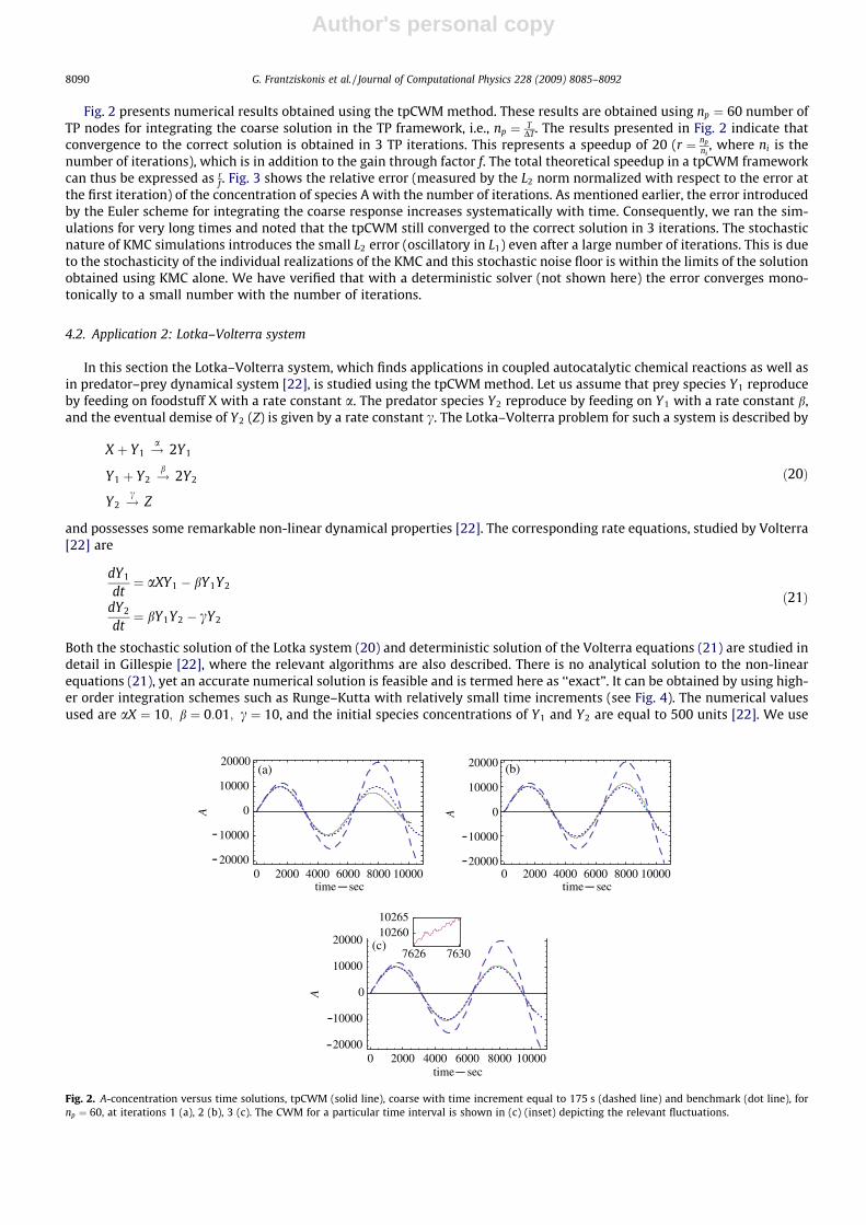
Fig. 2 presents numerical results obtained using the tpCWM method. These results are obtained using np ¼ 60 number ofTP nodes for integrating the coarse solution in the TP framework, i.e., np ¼ T
DT. The results presented in Fig. 2 indicate thatconvergence to the correct solution is obtained in 3 TP iterations. This represents a speedup of 20 (r ¼ np
ni, where ni is the
number of iterations), which is in addition to the gain through factor f. The total theoretical speedup in a tpCWM frameworkcan thus be expressed as r
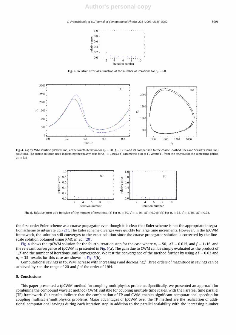
f . Fig. 3 shows the relative error (measured by the L2 norm normalized with respect to the error atthe first iteration) of the concentration of species A with the number of iterations. As mentioned earlier, the error introducedby the Euler scheme for integrating the coarse response increases systematically with time. Consequently, we ran the sim-ulations for very long times and noted that the tpCWM still converged to the correct solution in 3 iterations. The stochasticnature of KMC simulations introduces the small L2 error (oscillatory in L1) even after a large number of iterations. This is dueto the stochasticity of the individual realizations of the KMC and this stochastic noise floor is within the limits of the solutionobtained using KMC alone. We have verified that with a deterministic solver (not shown here) the error converges mono-tonically to a small number with the number of iterations.
4.2. Application 2: Lotka–Volterra system
In this section the Lotka–Volterra system, which finds applications in coupled autocatalytic chemical reactions as well asin predator–prey dynamical system [22], is studied using the tpCWM method. Let us assume that prey species Y1 reproduceby feeding on foodstuff X with a rate constant a. The predator species Y2 reproduce by feeding on Y1 with a rate constant b,and the eventual demise of Y2 (Z) is given by a rate constant c. The Lotka–Volterra problem for such a system is described by
X þ Y1 !a
2Y1
Y1 þ Y2 !b
2Y2
Y2 !c
Z
ð20Þ
and possesses some remarkable non-linear dynamical properties [22]. The corresponding rate equations, studied by Volterra[22] are
dY1
dt¼ aXY1 � bY1Y2
dY2
dt¼ bY1Y2 � cY2
ð21Þ
Both the stochastic solution of the Lotka system (20) and deterministic solution of the Volterra equations (21) are studied indetail in Gillespie [22], where the relevant algorithms are also described. There is no analytical solution to the non-linearequations (21), yet an accurate numerical solution is feasible and is termed here as ‘‘exact”. It can be obtained by using high-er order integration schemes such as Runge–Kutta with relatively small time increments (see Fig. 4). The numerical valuesused are aX ¼ 10; b ¼ 0:01; c ¼ 10, and the initial species concentrations of Y1 and Y2 are equal to 500 units [22]. We use
0 2000 4000 6000 8000 1000020000
10000
0
10000
20000
A
0 2000 4000 6000 8000 1000020000
10000
0
10000
20000
time sec
A
0 2000 4000 6000 8000 1000020000
10000
0
10000
20000
A
7626 7630
1026010265
-
--
--
-
_
time sec_
time sec_
(a) (b)
(c)
Fig. 2. A-concentration versus time solutions, tpCWM (solid line), coarse with time increment equal to 175 s (dashed line) and benchmark (dot line), fornp ¼ 60, at iterations 1 (a), 2 (b), 3 (c). The CWM for a particular time interval is shown in (c) (inset) depicting the relevant fluctuations.
8090 G. Frantziskonis et al. / Journal of Computational Physics 228 (2009) 8085–8092
Author's personal copy
the first-order Euler scheme as a coarse propagator even though it is clear that Euler scheme is not the appropriate integra-tion scheme to integrate Eq. (21). The Euler scheme diverges very quickly for large time increments. However, in the tpCWMframework, the solution still converges to the exact solution since the coarse propagator solution is corrected by the fine-scale solution obtained using KMC in Eq. (20).
Fig. 4 shows the tpCWM solution for the fourth iteration step for the case where np ¼ 50; DT ¼ 0:015, and f ¼ 1=16, andthe relevant convergence of tpCWM is presented in Fig. 5(a). The gain due to CWM can be simply evaluated as the product of1=f and the number of iterations until convergence. We test the convergence of the method further by using DT ¼ 0:03 andnp ¼ 35; results for this case are shown in Fig. 5(b).
Computational savings in tpCWM increase with increasing r and decreasing f. Three orders of magnitude in savings can beachieved by r in the range of 20 and f of the order of 1/64.
5. Conclusions
This paper presented a tpCWM method for coupling multiphysics problems. Specifically, we presented an approach forcombining the compound wavelet method (CWM) suitable for coupling multiple time scales, with the Parareal time parallel(TP) framework. Our results indicate that the combination of TP and CWM enables significant computational speedup forcoupling multiscale/multiphysics problems. Major advantages of tpCWM over the TP method are the realization of addi-tional computational savings during each iteration step in addition to the parallel scalability with the increasing number
2 4 6 8 100.0
0.2
0.4
0.6
0.8
1.0
iteration number
rela
tive
erro
r
Fig. 3. Relative error as a function of the number of iterations for np ¼ 60.
Fig. 4. (a) tpCWM solution (dotted line) at the fourth iteration for np ¼ 50; f ¼ 1=16 and its comparison to the coarse (dashed line) and ‘‘exact” (solid line)solutions. The coarse solution used in forming the tpCWM was for DT ¼ 0:015. (b) Parametric plot of Y2 versus Y1 from the tpCWM for the same time periodas in (a).
Fig. 5. Relative error as a function of the number of iterations. (a) For np ¼ 50; f ¼ 1=16; DT ¼ 0:015. (b) For np ¼ 35; f ¼ 1=16; DT ¼ 0:03.
G. Frantziskonis et al. / Journal of Computational Physics 228 (2009) 8085–8092 8091
Author's personal copy
of processors. The CWM corrects the coarse solution with the fine-scale solution by enabling an efficient interaction of thefine and coarse methods over the entire time interval instead of just at their common temporal nodes.
Acknowledgments
This research is sponsored by the Mathematical, Information, and Computational Sciences Division, Office of AdvancedScientific Computing Research, US Department of Energy. The work was partly performed at the Oak Ridge National Labo-ratory, which is managed by UT-Battelle, LLC under Contract No. De-AC05-00OR22725. The authors thank Dr. Stuart Dawat Oak Ridge National Laboratory, Sudib Mishra at University of Arizona, and Drs. Rodney Fox and Z. Gao at Iowa State Uni-versity for helpful discussions and feedback on the manuscript.
References
[1] L. Baffico, S. Bernard, Y. Maday, G. Turinici, G. Zerah, Parallel-in-time molecular-dynamics simulations, Physical Review E 66 (5) (2002).[2] G. Bal, A. Maday, A parareal time discretization for non-linear pdes with application to the pricing of an American put, in: Proceedings of the Workshop
on Domain Decomposition, Lecture Notes in Computational Science and Engineering, vol. 23, Springer, 2002, pp. 189–202.[3] G. Bal, Q. Wu, Symplectic parareal, in: Proceedings of the Workshop on Domain Decomposition, Lecture Notes in Computational Science and
Engineering, vol. 60, Springer, 2008, pp. 401–408.[4] F.A. Bornemann, Homogenization in Time of Singularly Perturbed Conservative Mechanical Systems, Springer-Verlag, Berlin, New York, 1998.[5] F.A. Bornemann, C. Schutte, Homogenization of hamiltonian systems with a strong constraining potential, Physica D 102 (1–2) (1997) 57–77.[6] F.A. Bornemann, C. Schutte, On the singular limit of the quantum-classical molecular dynamics model, SIAM Journal on Applied Mathematics 59 (4)
(1999) 1208–1224.[7] D. Cohen, E. Hairer, C. Lubich, Modulated fourier expansions of highly oscillatory differential equations, Foundations of Computational Mathematics 3
(4) (2003) 327–345.[8] W. E, B. Engquist, Z.Y. Huang, Heterogeneous multiscale method: a general methodology for multiscale modeling, Physical Review B 67 (9) (2003).[9] C. Farhat, M. Chandesris, Time-decomposed parallel time-integrators: theory feasibility studies for fluid, structure, and fluid–structure applications,
International Journal for Numerical Methods in Engineering 58 (2003) 1397–1434.[10] C. Farhat, J. Cortial, C. Dastillung, H. Bavestrello, Time-parallel implicit integrators for the near-real-time prediction of linear structural dynamics
responses, International Journal for Numerical Methods in Engineering 67 (2006) 697–724.[11] J. Fish, Bridging the scales in nano engineering and science, Journal of Nanoparticle Research 8 (2006) 557–594.[12] G. Frantziskonis, Multiscale characterization of materials with distributed pores and inclusions and application to crack formation in an aluminum
alloy, Probabilistic Engineering Mechanics 17 (2002) 359–367.[13] G. Frantziskonis, Wavelet-based multiscaling – application to material porosity and identification of dominant scales, Probabilistic Engineering
Mechanics 17 (2002) 349–357.[14] G. Frantziskonis, P. Deymier, Wavelet-based spatial and temporal multiscaling: bridging the atomistic and continuum space and time scales, Physical
Review B 68 (2) (2003).[15] G. Frantziskonis, P.A. Deymier, Wavelet methods for analysing and bridging simulations at complementary scales – the compound wavelet matrix and
application to microstructure evolution, Modelling and Simulation in Materials Science and Engineering 8 (5) (2000) 649–664.[16] G. Frantziskonis, A. Hansen, Wavelet-based multiscaling in self-affine random media, Fractals 8 (2000) 403–411.[17] G. Frantziskonis, S.K. Mishra, S. Pannala, S. Simunovic, C.S. Daw, P. Nukala, R.O. Fox, P.A. Deymier, Wavelet-based spatiotemporal multiscaling in
diffusion problems with chemically reactive boundary, International Journal for Multiscale Computational Engineering 4 (5–6) (2006) 755–770.[18] M.J. Gander, E. Hairer, Nonlinear convergence analysis for the parareal algorithm, in: Domain Decomposition Methods in Science and Engineering XVII,
Lecture Notes in Computational Science and Engineering, vol. 60, Springer, 2008.[19] M.J. Gander, S. Vandewalle, Analysis of the parareal time-parallel time-integration method, SIAM Journal on Scientific Computing 29 (2) (2007) 556–
578.[20] B. Garcia-Archilla, J.M. Sanz-Serna, R.D. Skeel, Long-time-step methods for oscillatory differential equations, SIAM Journal on Scientific Computing 20
(3) (1998) 930–963.[21] I. Garrido, B. Lee, G.E. Fladmark, M.S. Espedal, Convergent iterative schemes for time parallelization, Mathematics of Computation 75 (255) (2006)
1403–1428.[22] D.T. Gillespie, Exact stochastic simulation of coupled chemical-reactions, Journal of Physical Chemistry 81 (25) (1977) 2340–2361.[23] E. Hairer, C. Lubich, G. Wanner, Geometric Numerical Integration: Structure Preserving Algorithms for Ordinary Differential Equations, Springer Series
in Computational Mathematics, vol. 31, Springer-Verlag, 2002.[24] J.A. Izaguirre, S. Reich, R.D. Skeel, Longer time steps for molecular dynamics, Journal of Chemical Physics 110 (20) (1999) 9853–9864.[25] I.G. Kevrekidis, Equation-free coarse-grained multiscale computation: enabling microscopic simulators to perform system-level tasks, Communication
in Mathematical Sciences 14 (2003) 715.[26] B. Leimkuhler, S. Reich, Simulating Hamiltonian Dynamics, Cambridge University Press, 2004.[27] J.-L. Lions, Y. Maday, G. Turinici, A parareal in time discretization of pde’s, Comptes Rendus de l Academie des Sciences, Paris, Serie I 332 (2001) 661–
668.[28] C. Lubich, A variational splitting integrator for quantum molecular dynamics, Applied Numerical Mathematics 48 (3–4) (2004) 355–368.[29] Q. Ma, J.A. Izaguirre, R.D. Skeel, Verlet-i/r-respa/impulse is limited by nonlinear instabilities, SIAM Journal on Scientific Computing 24 (6) (2003) 1951–
1973.[30] K. Muralidharan, S.K. Mishra, G. Frantziskonis, P.A. Deymier, P. Nukala, S. Simunovic, S. Pannala, Dynamic compound wavelet matrix method for
multiphysics and multiscale problems, Physical Review E 77 (2) (2008).[31] R.M. Noyes, R.J. Field, Oscillatory chemical-reactions, Annual Review of Physical Chemistry 25 (1974) 95–119.[32] S. Reich, Multiple time scales in classical and quantum-classical molecular dynamics, Journal of Computational Physics 151 (1) (1999) 49–73.[33] J.M. Sanz-Serna, M.P. Calvo, Numerical Hamiltonian Problems, Chapman and Hall, London, 1994.[34] C. Schutte, F.A. Bornemann, Homogenization approach to smoothed molecular dynamics, Nonlinear Analysis – Theory Methods and Applications 30 (3)
(1997) 1805–1814.[35] M. Tuckerman, B.J. Berne, G.J. Martyna, Reversible multiple time scale molecular-dynamics, Journal of Chemical Physics 97 (3) (1992) 1990–2001.[36] A.V. Vasenkov, A.I. Fedoseyev, V.I. Kolobov, Computational framework for modeling of multi-scale processes, Computational and Theoretical
Nanoscience 3 (2006) 453–458.[37] D.D. Vvedensky, Multiscale modelling of nanostructures, Journal of Physics-Condensed Matter 16 (2004) R1537–R1576.
8092 G. Frantziskonis et al. / Journal of Computational Physics 228 (2009) 8085–8092