Author's personal copy - rwhite07.pages.tufts.edu · sure formulation results in a non-symmetric matrix. The non-sym-metry of the matrix can be removed using the velocity potential

Author's personal copy

Three-dimensional viscous finite element formulationfor acoustic fluid–structure interaction

Lei Cheng a,*, Robert D. White b, Karl Grosh c

a Department of Mechanical Engineering, 2350 Hayward Avenue, University of Michigan, Ann Arbor, MI 48109-2125, USAb Department of Mechanical Engineering, 200 College Avenue, Tufts University, Medford, MA 02155, USAc Department of Mechanical and Biomedical Engineering, 2350 Hayward Avenue, University of Michigan, Ann Arbor, MI 48109-2125, USA

a r t i c l e i n f o

Article history:Received 18 December 2007Received in revised form 4 April 2008Accepted 13 April 2008Available online 25 April 2008

Keywords:ViscousFinite element formulationAcoustic fluid–structure interaction

a b s t r a c t

A three-dimensional viscous finite element model is presented in this paper for the analysis of the acous-tic fluid–structure interaction systems including, but not limited to, the cochlear-based transducers. Themodel consists of a three-dimensional viscous acoustic fluid medium interacting with a two-dimensionalflat structure domain. The fluid field is governed by the linearized Navier–Stokes equation with the fluiddisplacements and the pressure chosen as independent variables. The mixed displacement/pressurebased formulation is used in the fluid field in order to alleviate the locking in the nearly incompressiblefluid. The structure is modeled as a Mindlin plate with or without residual stress. The Hinton–Huang’s 9-noded Lagrangian plate element is chosen in order to be compatible with 27/4 u/p fluid elements. Theresults from the full 3D FEM model are in good agreement with experimental results and other FEMresults including Beltman’s thin film viscoacoustic element [W.M. Beltman, P.J.M. Van der Hoogt,R.M.E.J. Spiering, H. Tijdeman, Implementation and experimental validation of a new viscothermal acous-tic finite element for acousto-elastic problems, J. Sound Vib. 216 (1) (1998) 159–185] and two and halfdimensional inviscid elements [A.A. Parthasarathi, K. Grosh, A.L. Nuttall, Three-dimensional numericalmodeling for global cochlear dynamics, J. Acoust. Soc. Am. 107 (2000) 474–485]. Although it is computa-tionally expensive, it provides a benchmark solution for other numerical models or approximations tocompare to besides experiments and it is capable of modeling any irregular geometries and materialproperties while other numerical models may not be applicable.

Published by Elsevier B.V.

1. Introduction

This paper deals with numerical modeling of three-dimensionalfluid–structure interaction problems using the finite elementmethod (FEM). Modeling fluid–structure interaction involves theanalysis of the fluid domain, the structure domain and the couplingbetween these two domains. While the structure domain is gener-ally described in a displacement formulation, there are a number ofFEM formulations available for modeling the fluid field dependingon the properties of the fluid. The fluid can usually be categorizedinto two different groups: the fluid flow and the acoustic fluid withsmall particle motions. For a general fluid flow problem, a fullNavier–Stokes equation is required to model the fluid field, whilefor the acoustic fluid, the fluid is often assumed to be linear andinviscid so that the fluid formulation can be greatly simplified.However, in a wide range of structural acoustic problems, the vis-cous effect plays an important role, especially in the system with a

thin fluid layer such as the trapped fluid hydromechanical cochlearmodel [25]. In these circumstances, the fluid viscosity is non-neg-ligible and should be included in the acoustic fluid model. In thispaper, we aim at developing a three-dimensional FEM formulationfor the analysis of the viscous acoustic fluid coupled with a flexibleboundary.

The commonly used fluid formulations include the pressure for-mulation [21], the potential formulation [7,18], the displacementformulation [15,11] and the combination of some of them [23,1].Choosing a scalar variable such as pressure for the fluid field signif-icantly reduces the problem size compared to the displacementformulation. For a transient analysis, it is well known that the pres-sure formulation results in a non-symmetric matrix. The non-sym-metry of the matrix can be removed using the velocity potentialformulation or the pressure–displacement potential formulationon the expense of an added damping matrix [7]. One significantdisadvantage of the pressure or potential formulation is that theyare developed for inviscid fluid only. The displacement formulationcan model a viscous fluid, and the coupling condition at the fluid–structure interface can be easily implemented. However, the dis-placement formulation in the frequency analysis suffers from the

0045-7825/$ - see front matter Published by Elsevier B.V.doi:10.1016/j.cma.2008.04.016

* Corresponding author. Tel.: +1 614 598 1732.E-mail addresses: [email protected] (L. Cheng), [email protected] (R.D. White),

[email protected] (K. Grosh).

Comput. Methods Appl. Mech. Engrg. 197 (2008) 4160–4172

Contents lists available at ScienceDirect

Comput. Methods Appl. Mech. Engrg.

journal homepage: www.elsevier .com/locate /cma


presence of the non-zero frequency modes with no physical mean-ing (i.e. spurious modes [15]), and it locks in the frequency analysisof a solid vibrating in a nearly incompressible fluid [19]. Recentlywe also found that the displacement formulation locks in the anal-ysis of a nearly incompressible fluid interacting with a flexibleboundary [26]. Many researchers have proposed improved formu-lations to solve this problem (a complete review on this matter canbe found in [1]) among which a displacement/pressure basedmixed formulation, developed by Bathe [1], has been demon-strated to have no spurious modes with the selection of the properelements. It is also proven to be effective in the analysis of incom-pressible or nearly incompressible media. For a three-dimensionalproblem, the mixed formulation has four degrees of freedom pernode in the fluid element, thus a higher computational burdencompared with the displacement based formulation. However,for a nearly incompressible fluid, the pressure degrees of freedomcan be condensed out in the element level, resulting in the samematrix size as in the displacement based formulation.

The viscous effect can also be included in the fluid modelapproximately under certain assumptions. Beltman et al. [2] pre-sented a viscothermal acoustic finite element model for acousto-elastic problems with thin layers. The model assumes that thepressure is constant across the layer thickness so that three-dimensional formulation is collapsed to two-dimensional. Belt-man’s model is only applicable when the viscous boundary layerthickness is comparable to the thickness of the layer. Bossartet al. [5] developed a hybrid numerical and analytical solutionfor thermo-viscous fluids, in which a modified acoustic boundarycondition is derived to account for the fluid viscosity using aboundary layer theory. The pressure formulation is used in thismodel since the viscous boundary condition is written in termsof pressure and its derivatives only. A similar non-dimensionalizedacoustic boundary condition was proposed by Holmes and Cole[13], although it was not implemented in the FEM model. Thesemodified boundary conditions were constructed under theassumption that the viscous boundary layer thickness is smallcompared to the dimension of the domain. To simulate the fre-quency response of a coupled fluid–structure system, the boundarylayer thickness could vary from big (at low frequencies) to small(at high frequencies) compared to the dimension of the system.Currently the viscous approximations only work at two extremecases but are not applicable to the problems with intermediateboundary layer thickness although it greatly simplifies the FEMformulation.

In this work, a fully coupled three-dimensional FEM formula-tion is derived for the analysis of acoustic fluid–structure interac-tion problems. The fluid is viscous and nearly incompressible.The fluid displacements are very small therefore a linear responsecan be assumed. The structure has a flat surface and is modeled asa plate with or without residual stress. The displacement pressurebased mixed formulation is used to model the fluid field to avoidthe locking behavior and to suppress the spurious modes. The cou-pling condition at the interface is such that the normal velocity andforce are continuous but the tangential velocities are negligible. Asimilar 3D coupled FEM model was developed by Figueroa et al. [8]to simulate the blood flow in the arteries. This study differs fromFigueroa’s work in the coupling condition at the fluid–structureinterface, the structural model and the elements used both in thestructure and fluid domains. This model could also find its applica-tion in the modeling of the cochlea and cochlear-based transduc-ers. There has been extensive research carried out over the last60 years attempting to understand the functioning of the cochleathrough experiments and mathematical models. A conventionalview of the cochlear mechanics can be found in [6] includingexperimental results and basic modeling techniques. Recent effortsin the cochlear modeling has been focused on developing a physi-

ologically realistic model of the cochlea and numerical meth-ods have become more popular due to their ability to deal withcomplicated structures. Giverlberg and Bunn [10] developed a fullthree-dimensional model of the curved cochlea using immersedboundary method [3]. The fluid is modeled as viscous and incom-pressible using nonlinear Navier–Stokes equation. Their modelshows the promise of large scale computational modeling applica-ble to study the cochlear mechanics, however, the computationalcost is very high compared to other 3D models. Parthasarathiet al. [21] proposed an inviscid fluid–structure coupled cochleamodel using the pressure formulation. In their model, the fluid do-main is meshed in 2D and a finite number of fluid modes is used inthe third dimension. The nature of this formulation (i.e. the modalsolution in one direction) limits its application in the viscous fluidmedium. Two different groups [9,4] used the commercial FEM soft-ware package ANSYS to study the passive cochlear mechanics, inwhich Böhnke and Arnold [4] developed a three-dimensionalfluid–structure interaction system with a curved cochlear duct.The fluid is considered inviscid and compressible. Gan et al. [9]built a 3D FEM model of the ear incorporated the ear canal, themiddle ear and the straightened cochlea. A more rapid solutioncan be obtained by a semi-analytic method known as Wentzel–Kramers–Brillouin (WKB) method [16,17,22,24]. Most WKB modelsin the cochlear mechanics only consider the first wave number intheir solutions, which may not capture the complete response ofthe cochlea [24]. Lim and Steele [17] extended the WKB model toinclude the fluid viscosity. Although the duct height and widthcan be slowly-varying in their model, it is still difficult to modela duct with any sudden change in the geometry, which is oftenseen in the cochlear-based transducers [26].

The organization of this paper is as follows. First we introducethe strong and weak forms for fluid domain, structure domainand the coupling between them. We then specify the interpola-tions used for fluid and structural elements, and the formulationsof the element stiffness matrix. Finally, the results from the 3DFEM model are given in comparison to experimental results andother FEM model results, followed by the conclusions.

2. Finite element framework

Fig. 1 shows a typical geometry of interior structural acousticsproblem where the viscous compressible fluid is bounded by solidwalls, part of which is occupied by a flat flexible structure. The ri-gid boundary is denoted as Cg and the flexible boundary is denotedas Cp. The governing equations for fluid domain and structure do-main are discussed next.

gΓ

Γ

Ω

p

Fig. 1. Geometry of coupled fluid–structure system.

L. Cheng et al. / Comput. Methods Appl. Mech. Engrg. 197 (2008) 4160–4172 4161


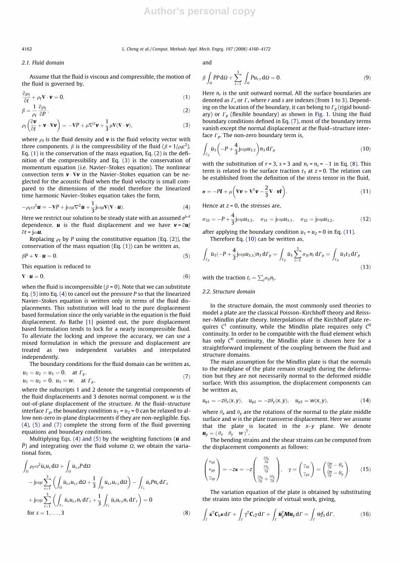
2.1. Fluid domain

Assume that the fluid is viscous and compressible, the motion ofthe fluid is governed by,

oqf

otþ qf$ � v ¼ 0; ð1Þ

b ¼ 1qf

oqf

oP; ð2Þ

qfovotþ v � $v

� �¼ �$P þ lr2v þ 1

3l$ð$ � vÞ; ð3Þ

where qf is the fluid density and v is the fluid velocity vector withthree components. b is the compressibility of the fluid (b = 1/qfc

2).Eq. (1) is the conservation of the mass equation, Eq. (2) is the defi-nition of the compressibility and Eq. (3) is the conservation ofmomentum equation (i.e. Navier–Stokes equation). The nonlinearconvection term v � $v in the Navier–Stokes equation can be ne-glected for the acoustic fluid when the fluid velocity is small com-pared to the dimensions of the model therefore the linearizedtime harmonic Navier–Stokes equation takes the form,

�qfx2u ¼ �$P þ jxlr2uþ 1

3jxl$ð$ � uÞ: ð4Þ

Here we restrict our solution to be steady state with an assumed ejxt

dependence. u is the fluid displacement and we have v = ou/ot = jxu.

Replacing qf by P using the constitutive equation (Eq. (2)), theconservation of the mass equation (Eq. (1)) can be written as,

bP þ $ � u ¼ 0: ð5Þ

This equation is reduced to

$ � u ¼ 0; ð6Þ

when the fluid is incompressible (b = 0). Note that we can substituteEq. (5) into Eq. (4) to cancel out the pressure P so that the linearizedNavier–Stokes equation is written only in terms of the fluid dis-placements. This substitution will lead to the pure displacementbased formulation since the only variable in the equation is the fluiddisplacement. As Bathe [1] pointed out, the pure displacementbased formulation tends to lock for a nearly incompressible fluid.To alleviate the locking and improve the accuracy, we can use amixed formulation in which the pressure and displacement aretreated as two independent variables and interpolatedindependently.

The boundary conditions for the fluid domain can be written as,

u1 ¼ u2 ¼ u3 ¼ 0; at Cg ;

u1 ¼ u2 ¼ 0; u3 ¼ w; at Cp;ð7Þ

where the subscripts 1 and 2 denote the tangential components ofthe fluid displacements and 3 denotes normal component. w is theout-of-plane displacement of the structure. At the fluid–structureinterface Cp, the boundary condition u1 = u2 = 0 can be relaxed to al-low non-zero in-plane displacements if they are non-negligible. Eqs.(4), (5) and (7) complete the strong form of the fluid governingequations and boundary conditions.

Multiplying Eqs. (4) and (5) by the weighting functions (�u andP) and integrating over the fluid volume X, we obtain the varia-tional form,Z

Xqfx

2�usus dXþZ

X

�us;sP dX

� jxlX3

r¼1

ZX

�us;rus;r dXþ 13

ZX

�us;rur;s dX

� ��Z

Cs

�usPns dCs

þ jxlX3

r¼1

ZCr

�usus;rnr dCr þ13

ZCr

�usur;snr dCr

� �¼ 0

for s ¼ 1; . . . ;3 ð8Þ

and

bZ

X

�PP dXþX3

r¼1

ZX

�Pur;r dX ¼ 0: ð9Þ

Here nr is the unit outward normal. All the surface boundaries aredenoted as Cs or Cr where r and s are indexes (from 1 to 3). Depend-ing on the location of the boundary, it can belong to Cg (rigid bound-ary) or Cp (flexible boundary) as shown in Fig. 1. Using the fluidboundary conditions defined in Eq. (7), most of the boundary termsvanish except the normal displacement at the fluid–structure inter-face Cp. The non-zero boundary term is,Z

Cp

�u3 �P þ 43

jxlu3;3

� �n3 dCp ð10Þ

with the substitution of r = 3, s = 3 and nr = ns = �1 in Eq. (8). Thisterm is related to the surface traction t3 at z = 0. The relation canbe established from the definition of the stress tensor in the fluid,

r ¼ �PI þ l $v þ $Tv � 23

$ � vI� �

: ð11Þ

Hence at z = 0, the stresses are,

r33 ¼ �P þ 43

jxlu3;3; r31 ¼ jxlu3;1; r32 ¼ jxlu3;2; ð12Þ

after applying the boundary condition u1 = u2 = 0 in Eq. (11).Therefore Eq. (10) can be written as,Z

Cp

�u3ð�P þ 43

jxlu3;3Þn3 dCp ¼Z

Cp

�u3

X3

r¼1

r3rnr dCp ¼Z

Cp

�u3t3 dCp

ð13Þ

with the traction ti ¼P

jrijnj.

2.2. Structure domain

In the structure domain, the most commonly used theories tomodel a plate are the classical Poisson–Kirchhoff theory and Reiss-ner–Mindlin plate theory. Interpolations of the Kirchhoff plate re-quires C1 continuity, while the Mindlin plate requires only C0

continuity. In order to be compatible with the fluid element whichhas only C0 continuity, the Mindlin plate is chosen here for astraightforward implement of the coupling between the fluid andstructure domains.

The main assumption for the Mindlin plate is that the normalsto the midplane of the plate remain straight during the deforma-tion but they are not necessarily normal to the deformed middlesurface. With this assumption, the displacement components canbe written as,

up1 ¼ �zhxðx; yÞ; up2 ¼ �zhyðx; yÞ; up3 ¼ wðx; yÞ; ð14Þ

where hx and hy are the rotations of the normal to the plate middlesurface and w is the plate transverse displacement. Here we assumethat the plate is located in the x–y plane. We denoteup ¼ hx hy wð ÞT.

The bending strains and the shear strains can be computed fromthe displacement components as follows:

�xx

�yy

cxy

0B@1CA ¼ �zj ¼ �z

ohxoxohy

oy

ohxoy þ

ohy

ox

0BB@1CCA; c ¼

cxz

cyz

!¼

owox � hx

owoy � hy

!: ð15Þ

The variation equation of the plate is obtained by substitutingthe strains into the principle of virtual work, giving,Z

C

�jTCbjdCþZ

C

�cTCscdCþZ

C

�uTpMup dC ¼

ZC

�wf3 dC; ð16Þ

4162 L. Cheng et al. / Comput. Methods Appl. Mech. Engrg. 197 (2008) 4160–4172


where Cp has been denoted as C for convenience. f3 is the transverseloading per unit area. Cb, Cs and M are defined as,

Cb ¼t3

12

Ex1�mxymyx

myxEx

1�mxymyx0

myxEx

1�mxymyx

Ey

1�mxymyx0

0 0 Gxy

26643775; Cs ¼ ktGxy

1 00 1

� �;

M ¼ �qpx2

t3

12 0 0

0 t3

12 00 0 t

264375;

ð17Þ

for an orthotropic plate. Ex, Ey and Gxy are the Young’s moduli andshear modulus. mxy and myx are the Poisson’s ratios. qp is the platedensity and t is the plate thickness. k is a constant to account forthe actual non-uniformity of the shearing stress and k is usually ta-ken to be 5/6 [1].

The boundary conditions for a simply-supported plate are:w = 0, hx and hy are free [14] at the edges.

2.3. Coupling between two domains

The coupling between the fluid and structure domains is realizedthrough the forcing terms. Since we have already neglected the in-plane displacements at the fluid–structure interface, the couplingoccurs only in the normal direction. We know that the surface trac-tion acting on the fluid due to the interaction with the structure isequal and opposite to the pressure loading on the structure by thefluid, i.e. t3 = �f3, and the continuity in the normal velocity at theinterface gives u3 = w. Using these two equations, we haveZ

C

�u3t3 dC ¼ �Z

C

�wf3 dC: ð18Þ

Hence the final form of the variational equations for the coupledsystem, if written in terms of the displacement components andpressure, is,Z

Xqfx

2�u1u1 dXþZ

X

�u1;1PdX� jxlZ

Xð�u1;1u1;1 þ �u1;2u1;2 þ �u1;3u1;3ÞdX

� 13

jxlZ

Xð�u1;1u1;1 þ �u1;2u2;1 þ �u1;3u3;1ÞdX¼ 0;Z

Xqfx

2�u2u2 dXþZ

X

�u2;2PdX� jxlZ

Xð�u2;1u2;1 þ �u2;2u2;2 þ �u2;3u2;3ÞdX

� 13

jxlZ

Xð�u2;1u1;2 þ �u2;2u2;2 þ �u2;3u3;2ÞdX¼ 0;Z

Xqfx

2�u3u3 dXþZ

X

�u3;3PdX� jxlZ

Xð�u3;1u3;1 þ �u3;2u3;2 þ �u3;3u3;3ÞdX

� 13

jxlZ

Xð�u3;1u1;3 þ �u3;2u2;3 þ �u3;3u3;3ÞdX�

ZC

�jTCbjdC

�Z

C

�cTCscdC�Z

C

�uTpMup dC¼ 0;

ð19Þalong with Eq. (9).

If the residual stress in the structure is non-negligible comparedto the bending effect, we should also include the tension effect inthe structure governing equation. Assume that the tensionsin the structure are Tx and Ty (they are not necessarily the same),the third equation in Eq. (19) is changed to,Z

Xqfx

2�u3u3 dXþZ

X

�u3;3P dX� jxlZ

Xð�u3;1u3;1 þ �u3;2u3;2

þ �u3;3u3;3ÞdX� 13

jxlZ

Xð�u3;1u1;3 þ �u3;2u2;3 þ �u3;3u3;3ÞdX

þZ

CðTx�u3;1u3;1 þ Ty�u3;2u3;2ÞdC�

ZC

�jTCbjdC�Z

C

�cTCscdC

�Z

C

�uTpMup dC ¼ 0: ð20Þ

We can see from the above equation that the structure degrees offreedom are only coupled to the fluid displacement in the z direc-tion, and the coupling only affects the fluid elements at the fluid–structure interface. There are two approaches to deal with thecoupling effects in the FEM discretization. The first one is to con-struct the fluid element at the fluid–structure interface separatelyso that its stiffness matrix can include the contribution from thestructure besides those from the fluid. The second one is to con-struct a coupling element at the interface to include only the cou-pling effect from the structure so that the fluid element at theinterface is the same as those in the domain. The second approachis used in this work and the main advantage for constructing a cou-pling element is that the fluid element at the interface does notchange with the mechanics of the structure. If the structure govern-ing equation or the coupling mechanics is changed, we only need togenerate a new coupling element. Next we will cover the basics forconstructing the fluid element, the structure element and the cou-pling element.

3. The choices of elements

Selecting the proper elements is essential to achieve accurateand converged results in the FEM formulation. In the fluid domain,we choose to use a 27/4 u/p mixed element [1] in which thedisplacement interpolation is tri-quadratic while the pressure islinearly interpolated. In the structure domain, the 9-nodedHinton–Huang’s element is used in order to be compatible withfluid element. The description of each element is detailed next.

3.1. Fluid elements

In the displacement/pressure based mixed formulation, weinterpolate not only the displacement but also the pressure. Sincethe pressure has the same order as the volume strain, its interpo-lation should be of lower order than the displacement. The sim-plest possible fluid element is a 8-noded brick element in whichthe displacement is linearly interpolated and the pressure is con-stant inside the element. This element is denoted as 8/1 u/p ele-ment and has been shown to be reasonably good, according toBathe [1]. However, it does not satisfy the inf–sup condition, a cri-terion to determine whether an element is stable and convergent[1], and also exhibits a spurious mode for a specific mesh with cer-tain boundary conditions. The 8/1 u/p element is actually equiva-lent to a 8-noded pure displacement based element with reducedintegration on the compressibility term [14], which exhibits lock-ing behavior at low frequencies for the example problem shownin this paper (see Section 5 for more details).

Considering a higher-order displacement interpolation such astri-quadratic interpolation (corresponding to a 27-noded elementfor the displacement), the pressure interpolation has severalchoices including a constant, linear or trilinear interpolations.The study [1] shows that the element with tri-quadratic displace-ment and linear pressure gives the best overall performanceamong these choices and it is named as 27/4 u/p mixed elementsince the pressure interpolation has four unknowns:P = p0 + p1x + p2y + p3z.

To obtain the governing finite element equations for the fluid,here we will show the formulation of the stiffness matrix for onesingle element. Assembling the global matrix from the elementmatrix can be performed in a standard manner. For a 27/4 u/p ele-ment, we assume that the displacement and pressure interpola-tions are,

u ¼ Nuu; P ¼ NpbP ð21Þ

with



Nu ¼N1

u 0 0 N2u 0 0 � � � N27

u 0 0

0 N1u 0 0 N2

u 0 � � � 0 N27u 0

0 0 N1u 0 0 N2

u � � � 0 0 N27u

264375;

u ¼ u11 u1

2 u13 u2

1 u22 u2

3 � � � u271 u27

2 u273

� �T;bP ¼ P0 P1 P2 P3½ �T;

ð22Þ

where N1u to N27

u are the shaping functions for a 27-noded trilinearelement and u is the nodal displacement vector. The superscriptand subscript in u2

1 denote the nodal number and the displacementcomponent, respectively (e.g., u2

1 is the fluid displacement in the xdirection at node 2). bP is the unknown pressure vector. Note thatbP does not correspond to any nodal pressure. Using this interpola-tion, the pressure is continuous inside the element but discontinu-ous across the element. Substituting the interpolations into the fluidvariational equation (Eq. (19)), we can obtain the element stiffnessmatrix,

Ke ubP� �

¼Ke

uu Keup

Kepu Ke

pp

" #ubP

� �¼

R0

� �; ð23Þ

where

Keup ¼ ðK

epuÞ

T ¼Z

XBT

vNp dX;

Kepp ¼ b

ZX

NTpNp dX

ð24Þ

and

Bv ¼ oN1u

oxoN1

uoy

oN1u

ozoN2

uox � � �

oN27u

oz

h i: ð25Þ

The expression for Keuu can be obtained from the fluid governing

equation directly and is omitted here. Since the pressure degreesof the freedom bP are only pertain to one element, we can solvethe pressure unknowns using the second equation in Eq. (23),bP ¼ �ðKe

ppÞ�1Ke

puu; ð26Þ

substituting this equation into the first equation in Eq. (23), we ob-tain the new element stiffness matrix which is only related to thenodal displacement:

Ke ¼ Keuu � Ke

upðKeppÞ�1ðKe

puÞ; ð27Þ

so that the pressure degrees of freedom are condensed out on theelement level. Note this stiffness matrix is different from the onein the pure displacement based formulation although the un-knowns in the final equation are both nodal displacements. Thepressure unknowns are canceled out in the weak form and the pres-sure is interpolated independently. The forcing term in the fluidvariational equation will be considered in the next section in thecoupling elements.

4. Structural/coupling element

Similar to the fluid element, the pure displacement based plateelements tend to be overly constrained and exhibit a strong artifi-cial stiffening in the thin plate limit. To alleviate the effect of shearlocking in the plate element, different interpolations are used forthe bending and shear strains. In order to be compatible withthree-dimensional 27-noded fluid element, the structural elementshould have 9 nodes with bilinear interpolation for the transversedisplacement. There are two groups of 9-noded structural ele-ments shown to be efficient and reliable with a mixed interpola-tion for bending and shear strains: MITC9 element (MITC standsfor mixed interpolation of tensorial components) [1] and Hinton–Huang’s 9-noded plate element [12]. Unfortunately the MITC9element uses a serendipity type interpolation for transverse dis-

placement (8 nodes for the displacement and 9 nodes for sectionrotations) which makes it incompatible with the fluid element. Inthis paper, we use Hinton–Huang’s Lagrangian element for thecoupled analysis.

Following the general methodology proposed by Onate et al.[20] for deriving Hinton and Huang’s plate element, the shearstrains are interpolated independently with the following form:

cn ¼ a1 þ a2nþ a3gþ a4ngþ a5g2 þ a6ng2;

cg ¼ b1 þ b2nþ b3gþ b4ngþ b5n2 þ b6gn2

ð28Þ

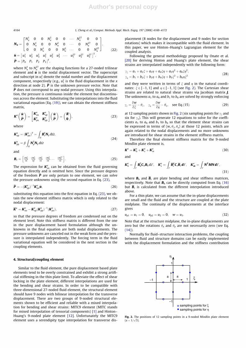
and they were written in terms of n and g in the natural coordi-nates: n 2 [�1, 1] and g 2 [�1, 1] (see Fig. 2). The Cartesian shearstrains are related to natural shear strains via Jacobian matrix J.The unknowns a1 to a6 and b1 to b6 are solved by strongly enforcing

cn ¼owon� hn; cg ¼

owog� hg; see Eq:ð15Þ ð29Þ

at 12 sampling points shown in Fig. 2 (six sampling points for cn andsix for cg). This will generate 12 equations to solve for the coeffi-cients a1 to a6 and b1 to b6 so that the element shear strains canbe expressed in terms of (w, hn, hg) at those 12 points, which areagain related to the nodal displacements and no more unknownsare introduced for shear strains in the element stiffness matrix.

Therefore the final element stiffness matrix for the 9-nodedMindlin plate element is,

Ke ¼ Keb þ Ke

s þ Kem ð30Þ

and

Keb ¼

ZC

BTbCbBb dC; Ke

s ¼Z

CBT

s CsBs dC; Kem ¼

ZC

NT MN dC;

ð31Þ

where Bb and Bs are plate bending and shear stiffness matrices,respectively. Note that Bb can be directly computed from Eq. (16)but Bs is calculated from the different interpolation introducedabove.

For a thin plate, we can assume that the in-plane displacementsare small and the fluid and the structure are coupled at the platemidplane. The continuity of the displacements at the interfacegives

up1 ¼ u1 ¼ 0; up2 ¼ u2 ¼ 0; w ¼ u3: ð32Þ

Note that at the structure midplane, the in-plane displacements arezero but the rotations hx and hy are not necessarily zero (see Eq.(14)).

Normally for fluid–structure interaction problems, the couplingbetween fluid and structure domains can be easily implementedwith the displacement formulation and the stiffness contribution

–1 1

1

aa ξ

η

sampling points for ξsampling points for η

–1

Fig. 2. The positions of 12 sampling points in a 9-noded Mindlin plate element(a ¼ 1=

ffiffiffi3p

).



from the structure can be directly added to the fluid stiffness ma-trix at the corresponding nodes at the interface. However, this isnot the case in our problem since there is no direct coupling be-tween (u1, u2) and (hx, hy) at the interface. We need to construct anew element which can couple the structural degrees of freedom(w, hx, hy) to the fluid degrees of freedom (u1, u2, u3) at the interfaceand also account for the plate stiffness contribution in the varia-tional equation (Eq. (19)). The coupling element has 18 nodes with9 structural nodes on the bottom plane (numbered 1–9) and 9 fluidnodes on the top (numbered 10–18), as shown in Fig. 3. Since allthe nodes are located at the plate midplane and the element haszero thickness, node 1 and node 10 have exactly the same coordi-nates, so do node 2 and node 11, and etc. The degrees of freedomfor the bottom nodes are (hx, hy) and (u1, u2, u3) for the top nodes.Note that the bottom nodes only have two degrees of freedom in-stead of three in the plate element, because at the interface wehave u3 = w so only one of them needs to be included in the ele-ment. The nodal degrees of freedom for one single coupling ele-ment is,

uc ¼ h1x h1

y � � � h9x h9

y u101 u10

2 u103 � � � u18

1 u182 u18

3

h i:

ð33Þ

With the use of the new element, at the interface we have fluidelement which is the same as the ones in the domain and also azero-thickness coupling element with top 9 nodes the same asfluid nodes and bottom 9 nodes for plate rotations. The third equa-tion in Eq. (19) shows that the deformation of the structure is cou-pled to the fluid domain as a boundary condition and the couplingonly occurs between hx, hy and u3 (i.e. w). The coupling elementstiffness matrix Ke

c is just an expansion of the stiffness matrix forstructural elements with extra zeros at the rows and columns re-lated to u1 and u2,

Kec ¼

Kehh Ke

hw

Kewh Ke

ww

" #ð34Þ

with

Kehh ¼

k11 k12 k14 k15 � � � k1;26

k22 k24 k25 � � � k2;26

k44 k45 � � � k4;26

symm: k55 � � � k5;26;

. .. ..

.

k26;26

26666666664

3777777777518�18

; ð35Þ

Keww ¼

0 0 0 0 0 0 � � � 00 0 0 0 0 � � � 0

k33 0 0 k36 � � � k3;27

0 0 0 � � � 0symm: 0 0 � � � 0

k66 � � � k6;27

. ..

� � �k27;27

2666666666666664

377777777777777527�27

; ð36Þ

Kehw ¼ ðK

ewhÞ

T ¼

0 0 k13 0 0 k16 � � � k1;27

0 0 k23 0 0 k26 � � � k2;27

0 0 k43 0 0 k46 � � � k4;27

0 0 k53 0 0 k56 � � � k5;27

..

. ... ..

. ... ..

. ... ..

. ...

0 0 k26;3 0 0 k26;6 � � � k26;27

26666666664

3777777777518�27

; ð37Þ

where kij is the (i, j)th component of the plate element stiffness ma-trix Ke (see Eq. (30)). We can see that in the coupling element stiff-ness matrix, hx and hy are not coupled to u1 and u2, because thecoupling element is constructed on the plate midplane and the in-plane displacements for the fluid and structure are all zero at theinterface. As an alternative, Figueroa et al. [8] proposed a differentcoupling element in which they neglect the variations of the struc-ture in-plane displacements across the thickness so that the cou-pling conditions at the interface can be written as

up1 ¼ u1; up2 ¼ u2; w ¼ u3;

f1 ¼ �t1; f 2 ¼ �t2; f 3 ¼ �t3ð38Þ

and this slightly modifies the variational statement in Eq. (19).

5. Results and discussion

In this section, some specific results for three-dimensional FEMcomputations of fluid–structure interaction are given using the for-mulation described in this paper. These results are compared toexperimental results for steady state vibration of microscalefluid–structure systems as well as to computational resultsachieved using two lower-dimensional finite element schemes.

Both of the lower-dimensional finite element schemes includefull fluid–structure coupling. The first of these was described byParthasarathi et al. [21]. It is an inviscid, harmonic, pressure-basedmodel that uses a full fluid mesh for pressure in two dimensions,but a finite number of inviscid fluid modes in the third dimension.A single structural cross-mode shape is used, and the structuralmotion is fully meshed in one dimension only. We refer to thisas 2.5D FEM. The second two-dimensional scheme is a thin-filmviscoacoustic model taken from the work of Beltman et al. [2]. Thisapproach uses a two-dimensional mesh for both the fluid andstructural vibration, but assumes that the fluid film is very thin,resulting in a single pressure dependent variable for the fluid. Fluidviscosity is included in Beltman’s model.

The 3D FEM model described in this paper can be used in manyacoustic fluid–structure interaction problems in which the linear-ized Navier–Stokes equation is applicable. For an example of thecapabilities, we choose to compare our model results to thefluid–structure traveling waves in hydromechanical cochlear mod-els. The authors have designed, built and tested a number of suchmodels. Fig. 4 shows the typical geometry of the cochlear-basedtransducers. The fluid-filled cochlear duct is idealized as a singlerectangular fluid filled duct. A flexible structure, which mimicsthe flexible basilar membrane (BM) in the cochlea, occupies partof the bottom wall. The width of this membrane structure variesalong the length of the duct. The acoustic input to the system isapplied through another rectangular flexible membrane on the

Fluid Element

Structure Element

Coupling Element

1 5 2

6974

8

3

11

12

15

16

1410

17

13

18z=0

z=0

z=0

z=0

Fig. 3. Fluid element, structure element and coupling element at the fluid–struct-ure interface.



bottom wall, which we refer to as the ‘‘input membrane”. All otherwalls of the duct are considered to be rigid. We define the coordi-nate axes as follows: the x-axis extends longitudinally along theduct length. The y-axis is oriented across the width of the mem-brane, thus the membrane lies in the x–y plane. The z-axis is nor-mal to the membrane, that is, it defines the height of the duct. Thegeometry is symmetric about the x–z plane, thus only half of thegeometry is modeled with symmetry boundary conditions speci-fied on y = 0. The geometric and material properties used in theexample problems are given in Fig. 5 and Table 1.

The fluid chamber is micromachined from glass and anodicallybonded to a thick silicon die which supports the membrane struc-tures. The basilar membrane is a composite structure composed ofa 300 nm thick stoichiometric silicon nitride thin film etched intoparallel beams overlayed with a 1.4 lm thick polyimide layer(PI2737 from HD Microsystems, Parlin, NJ). This results in a ten-sioned orthotropic structure with a tension of approximately240 N/m in the y direction and 30 N/m in the x direction, as deter-mined by wafer curvature measurements on the unpatternedfilms. The basilar membrane structure is 30 mm long, and tapersexponentially in width from 0.14 mm to 1.82 mm, as shown inFig. 5. The input membrane is a rectangle, 1.1 mm � 2.1 mm. Thefluid duct is filled with silicone oil with a viscosity of 5 cSt and adensity of 911 kg/m3. Fluid–structure traveling waves and struc-tural vibration are excited by exposing the input membrane toair borne sound delivered by a tweeter. Measurement of the vibra-tion response of the basilar membrane is carried out at steady stateusing a microscale scanning laser vibrometer and a lock-inamplifier.

Fig. 6a shows the measured magnitude of structure displace-ment normalized to the driving pressure from the input membraneat 4.2 kHz, 12 kHz and 35 kHz. These results have been publishedpreviously in [25]. The corresponding model results calculatedfrom the mixed 3D FEM formulation are shown in Fig. 6b. For allthree frequencies, the fluid domain is meshed using 603 nodes inthe length direction, 15 nodes in the width direction and 13 nodesin the height direction. The basilar membrane is meshed using501 � 7 uniform grid and the input membrane is meshed using43 � 11 uniform grid. The model correctly captures the locationof the maximum response and the wave decay after the peak aswell as making a good prediction of the magnitude of the response.Any discrepancies between the modeled and measured responsemagnitude can be attributed to uncertainties in the driving pres-sure, which cannot be measured exactly at the input membrane.There is also very good agreement between experimental andFEM model results showing the phase of the structural vibrationalong the membrane centerline (along the x-axis) at three frequen-cies, as shown in Fig. 7. Note that for this system, the compliance of

the BM is about two to three orders of magnitude lower than thatof the real cochlea [25], so that the bandwidth of the model shiftstowards slightly ultrasonic regime (4–35 kHz).

For comparison, Fig. 8 shows the computational results from apure displacement based 3D finite element formulation. This infe-rior model uses an 8-noded brick element in the fluid domain withtrilinear interpolation for the displacement. The FEM mesh usesthe same number of the nodes as in the above example (whichmeans that the number of the elements is doubled in each direc-tion). For the terms involving the fluid compressibility, a one pointquadrature rule is applied, while the other terms use 2 � 2 � 2Gaussian quadrature. This selective reduced integration schemeis used in an attempt to alleviate the element locking due to thenearly incompressible fluid. However, at the low frequencies suchas 4.2 kHz, the pure displacement based formulation still locks ifcompared with the results from the mixed FEM model in Fig. 6b.At 12 kHz, it predicts a smaller displacement magnitude than thatof the mixed model and the location of the peak is more towardsthe base of the duct. As mentioned earlier, this 8-noded displace-ment based formulation is equivalent to an 8/1 displacement/pres-sure mixed formulation and does not satisfy inf–sup condition,meaning the element is not stable. Although it is very simple toimplement and gives a good prediction of the response at some fre-quencies, such as 35 kHz, the behavior of this formulation is notpredictable as we do not know when it will lock and producemeaningless results. In contrast, the 27/4 mixed 3D formulation

y

z

Basilar Membrane

Fluid Filled Duct

Input Membrane

x

Fig. 4. Geometry of coupled fluid–structure system.

z

x

A’A

3.125

0.11

37.25

y

Unit: mm

0.07

A–A’

2 301.11 3.15

1.05

0.91

Fig. 5. The dimension of the duct and the structure. The thickness of the structure is0.32 lm.

Table 1Material properties for the example problem

Symbols Value Unit Physical meaning

qf 911 kg/m3 Fluid densityc 1000 m/s Fluid wave speedl 5 cSt Fluid viscosityqp 3.6 � 10�3 kg/m2 Plate area densityEx 20 GPa Young’s modulus in xEy 160 GPa Young’s modulus in ym 0.3 Poisson’s ratioTx 30 N/m Tension in xTy 240 N/m Tension in yg 0.01 Structural damping



described in this paper gives excellent results at all frequenciesalthough the computational cost is higher.

The convergence of the 3D mixed FEM model is discussed next.As an example, Fig. 9 shows the structure displacement at 4.2 kHzusing four different meshes: the original mesh we used in theFig. 6, doubling the elements in the length, width and height direc-tion respectively. Due to the limitation of our current computa-tional resources (maximum memory 64 GB), it is not feasible tohave even more refined mesh without exceeding the memoryrequirement. However, the converged results in Fig. 9 suggests thatthe mesh resolution in the above example is sufficient.

Fig. 10 shows the comparison of the structure displacementcomputed from the 2.5D FEM [21] model and the 3D FEM modelat 12 kHz (Fig. 10a) and 35 kHz (Fig. 10b), respectively. For the3D FEM model, the fluid domain is again meshed using 603 nodesin the x direction, 15 nodes in the y direction and 13 nodes in the zdirection, the basilar membrane is meshed using 501 � 7 uniformgrid and the input membrane is meshed using 43 � 11 unform

0 5 10 15 20 25 300

0.1

0.2

0 5 10 15 20 25 300

0.1

0.2

Dis

p. M

agni

tude

(nm

/Pa)

0 5 10 15 20 25 300

0.1

0.2

X (mm)

4.2kHz

12kHz

35kHz

0 5 10 15 20 25 300

0.05

0.1

0 5 10 15 20 25 300

0.02

0.04

0.06

Dis

p. M

agni

tude

(nm

/Pa)

0 5 10 15 20 25 300

0.02

0.04

X (mm)

12kHz

4.2kHz

35kHz

a b

Fig. 6. The magnitude of structure displacement at three different frequencies: (a) the experimental results [25]; (b) the model results from the displacement/pressure mixedformulation which uses the 27/4 u/p element for the fluid and the 9-noded Hinton–Huang’s element for the structure. Note that due to optical constraints the entire basilarmembrane is not imaged in the experiments; the data starts at 4 mm from the narrow end of the device.

0 5 10 15 20 25 30–40

–35

–30

–25

–20

–15

–10

–5

0

5

X (mm)

Pha

se (

radi

ans)

4.2kHz

12kHz

35kHz

Fig. 7. Comparison of the phase of structure displacement at three different freq-uencies between the experimental results (dashed line) and the model results (solidline). The experimental data are reference to the phase at 4 mm from the narrowend of the device.

0 5 10 15 20 25 300

0.02

0.04

X (mm)

0 5 10 15 20 25 300

0.01

0.02

0 5 10 15 20 25 300

0.02

0.04

Dis

p. M

agni

tude

(nm

/Pa)

4.2kHz

12kHz

35kHz

Fig. 8. The magnitude of structure displacement calculated from a pure displace-ment based formulation with 8-noded fluid elements and selectively reduced int-egration scheme.

0 5 10 15 20 25 300

0.01

0.02

0.03

0.04

0.05

0.06

0.07

0.08

0.09

0.14.2kHz

BM Length (mm)

Nor

mal

ized

BM

Dis

p. (

nm/P

a)

originaldouble x elementsdouble z elementsdouble y elements

Fig. 9. The magnitude of structure displacement at 4.2 kHz calculated by mixed 3DFEM formulation using four different meshes.



grid. For the 2.5D FEM model, the fluid domain is meshed using603 x nodes and 42 z nodes. Eight cross-modes is used in the ydirection. The structure has 501 nodes in the x direction with onlyone cross-mode. The 2.5D FEM formulation uses the modal solu-tion in the y direction with a pressure formulation and thereforeit only needs a two-dimensional mesh in the x–z plane, big savingsin the computational cost but it can only model inviscid fluid, amajor drawback. For a fair comparison we must therefore setl = 0 in the 3D FEM model and instead add structural damping inan ad hoc fashion (g = 0.05) to reduce the reflections from theboundary. The results in Fig. 10b show that there are strong stand-ing waves formed at the end of the structure at 12 kHz, indicatingthat the structure damping is still not high enough to suppress allthe reflections. The mesh resolution is about 11 nodes per wave-length at the place where the wavelength is shortest. The resultsfrom the 2.5D FEM model are in a fairly good agreement with 3DFEM results at both frequencies, although there are slight differ-ences in the peak and magnitude of the structure displacements.The discrepancy could be a result of the presence of the highercross-modes in the input membrane, as shown in Fig. 11. Thewidth of the input membrane is two times larger than its length,so we expect to see higher modes appearing first in the widthdirection. At 35 kHz, Fig. 11b clearly shows that the displacementin the input membrane has broken into higher cross-modes,

although the slender-shaped BM is still dominated by the firstcross-mode (Fig. 12). It is, of course, possible for the BM to havehigher cross-modes at higher frequencies, and those modes willfirst appear at the wider end of the structure.

Fig. 13 shows the structure displacement calculated from Belt-man’s thin film viscothermal acoustic model and the 3D FEM mod-el at 12 kHz. For the 3D FEM model, the fluid domain is meshedusing 603 x nodes, 15 y nodes and 21 z nodes, and the basilar mem-brane and the input membrane are meshed using 501 � 7 and43 � 11 uniform grid, respectively. In the Beltman’s thin filmmodel, only two-dimensional mesh in the x–y plane is needed,and in this example, the mesh is the same as that of the 3D FEMmodel in the x–y plane. As mentioned before, Beltman’s model as-sumes that the pressure is constant across the height of the duct,and thus it may only be applied to structural acoustic systems withthin gaps. The boundary layer thickness, d ¼

ffiffiffiffiffiffiffiffiffiffiffiffiffil=qfx

p, is required to

be of the same magnitude or larger than the height of the duct. Inorder to test the effects of violating this requirement, a model casewith 474 lm high duct is compared with the results for a 110 lmhigh duct. The results appear in Fig. 13. Fig. 13a shows an excellentagreement between Beltman’s model and 3D FEM model with thesmaller duct height, while in Fig. 12b, the Beltman’s model seemsto provide less damping to the system so that the displacementmagnitude is higher. The inaccuracy in the displacement predic-

0 5 10 15 20 25 300

0.02

0.04

0.06

0.08

0.1

0.12

BM Length (mm)

Nor

mal

ized

BM

Dis

p. (

nm/P

a)

2.5d FEM3d FEM

0 5 10 15 20 25 300

0.01

0.02

0.03

0.04

0.05

BM Length (mm)

Nor

mal

ized

BM

Dis

p. (

nm/P

a)

2.5d FEM3d FEM

a b

Fig. 10. The comparison of the structure displacement calculated from 2.5D FEM model and 3D FEM model using 27/4 u/p fluid element and Hinton–Huang’s structuralelement: (a) response at 12 kHz; (b) response at 35 kHz. Fluid is inviscid, and pure tensioned membrane model is used for the structure with structural damping g = 0.05.

Fig. 11. The two-dimensional view of the displacement of the input membrane calculated from 3D FEM model: (a) response at 12 kHz; (b) response at 35 kHz.



Fig. 12. The two-dimensional view of the BM displacement calculated from 2.5D FEM model and 3D FEM model: (a) response at 12 kHz; (b) response at 35 kHz.

0 5 10 15 20 25 300

0.01

0.02

0.03

0.04

0.05

0.06

BM Length (mm)

Nor

mal

ized

BM

Dis

p. (

nm/P

a)

beltman3d FEM

0 5 10 15 20 25 300

0.1

0.2

0.3

0.4

0.5

0.6

0.7

Length (mm)

Nor

mal

ized

BM

Dis

p. (

nm/P

a)beltman3d FEM

a b

Fig. 13. The comparison of the structure displacement between Beltman’s FEM model and 3D FEM model using 27/4 u/p fluid element and Hinton–Huang’s structuralelement at 12 kHz: (a) duct height is 110 lm; (b) duct height is 475 lm. In Beltman’s FEM model, 501 � 7 uniform grid is used for plate. In 3D FEM, 501 � 7 uniform grid isused for the plate, and 603 x nodes, 15 y nodes and 21 z nodes are used for the fluid.

1 1.2 1.4 1.6 1.8 2 2.20

20

40

60

80

100

120

Normalized Ux

Hei

ght (

μm) x=1.5

x=3

x=20

x=25

x=30

Beltman

a b

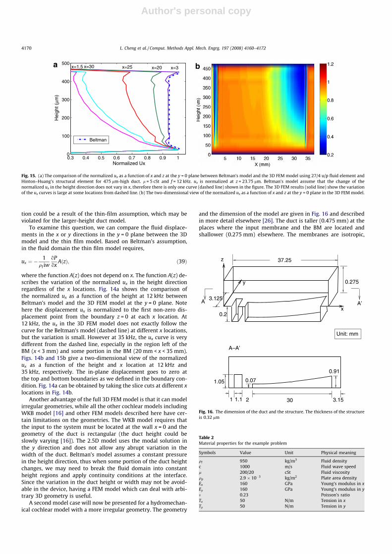
Fig. 14. (a) The comparison of the normalized ux as a function of x and z at the y = 0 plane between Beltman’s model and the 3D FEM model for 110 lm-high duct. ux isnormalized at z = 5.5 lm. l = 5 cSt and f = 12 kHz. Beltman’s model assume that the change of the normalized ux in the height direction does not vary in x, therefore there isonly one curve (dashed line) shown in the figure. The 3D FEM results (solid line) show there are some variation in x, but the variation is small in this case. (b) The two-dimensional view of the normalized ux as a function of x and z at the y = 0 plane in the 3D FEM model.



tion could be a result of the thin-film assumption, which may beviolated for the larger-height duct model.

To examine this question, we can compare the fluid displace-ments in the x or y directions in the y = 0 plane between the 3Dmodel and the thin film model. Based on Beltman’s assumption,in the fluid domain the thin film model requires,

ux ¼ �1

qf iwoPox

AðzÞ; ð39Þ

where the function A(z) does not depend on x. The function A(z) de-scribes the variation of the normalized ux in the height directionregardless of the x locations. Fig. 14a shows the comparison ofthe normalized ux as a function of the height at 12 kHz betweenBeltman’s model and the 3D FEM model at the y = 0 plane. Notehere the displacement ux is normalized to the first non-zero dis-placement point from the boundary z = 0 at each x location. At12 kHz, the ux in the 3D FEM model does not exactly follow thecurve for the Beltman’s model (dashed line) at different x locations,but the variation is small. However at 35 kHz, the ux curve is verydifferent from the dashed line, especially in the region left of theBM (x < 3 mm) and some portion in the BM (20 mm < x < 35 mm).Figs. 14b and 15b give a two-dimensional view of the normalizedux as a function of the height and x location at 12 kHz and35 kHz, respectively. The in-plane displacement goes to zero atthe top and bottom boundaries as we defined in the boundary con-dition. Fig. 14a can be obtained by taking the slice cuts at different xlocations in Fig. 14b.

Another advantage of the full 3D FEM model is that it can modelirregular geometries, while all the other cochlear models includingWKB model [16] and other FEM models described here have cer-tain limitations on the geometries. The WKB model requires thatthe input to the system must be located at the wall x = 0 and thegeometry of the duct is rectangular (the duct height could beslowly varying [16]). The 2.5D model uses the modal solution inthe y direction and does not allow any abrupt variation in thewidth of the duct. Beltman’s model assumes a constant pressurein the height direction, thus when some portion of the duct heightchanges, we may need to break the fluid domain into constantheight regions and apply continuity conditions at the interface.Since the variation in the duct height or width may not be avoid-able in the device, having a FEM model which can deal with arbi-trary 3D geometry is useful.

A second model case will now be presented for a hydromechan-ical cochlear model with a more irregular geometry. The geometry

and the dimension of the model are given in Fig. 16 and describedin more detail elsewhere [26]. The duct is taller (0.475 mm) at theplaces where the input membrane and the BM are located andshallower (0.275 mm) elsewhere. The membranes are isotropic,

0.3 0.4 0.5 0.6 0.7 0.8 0.9 10

100

200

300

400

500

Normalized Ux

Hei

ght (

μm)

x=1.5 x=30 x=25 x=20 x=3

Beltman

a b

Fig. 15. (a) The comparison of the normalized ux as a function of x and z at the y = 0 plane between Beltman’s model and the 3D FEM model using 27/4 u/p fluid element andHinton–Huang’s structural element for 475 lm-high duct. l = 5 cSt and f = 12 kHz. ux is normalized at z = 23.75 lm. Beltman’s model assume that the change of thenormalized ux in the height direction does not vary in x, therefore there is only one curve (dashed line) shown in the figure. The 3D FEM results (solid line) show the variationof the ux curves is large at some locations from dashed line. (b) The two-dimensional view of the normalized ux as a function of x and z at the y = 0 plane in the 3D FEM model.

37.25

0.07

A–A’

2 301.11 3.15

1.05

0.91

x

3.125

y 0.275

0.2

A’A

z

Unit: mm

Fig. 16. The dimension of the duct and the structure. The thickness of the structureis 0.32 lm

Table 2Material properties for the example problem

Symbols Value Unit Physical meaning

qf 950 kg/m3 Fluid densityc 1000 m/s Fluid wave speedl 200/20 cSt Fluid viscosityqp 2.9 � 10�3 kg/m2 Plate area densityEx 160 GPa Young’s modulus in xEy 160 GPa Young’s modulus in ym 0.23 Poisson’s ratioTx 50 N/m Tension in xTy 50 N/m Tension in y



and made from a laminate of silicon nitride/doped polysilicon/sil-icon nitride (0.1 lm/1 lm/0.1 lm). The structure is still microma-chined from silicon and glass and anodically bonded together.Silicone oil is still used as the fluid medium. The estimated mate-rial properties for the device are given in Table 2. Fig. 17a showsthe computed BM displacement at 10 kHz for two different viscos-ities: l = 200 cSt and l = 20 cSt. The BM displacement exhibitssteeper cut-off after the resonance peak for the higher viscosity,but the magnitude is smaller (10 dB lower compared to 20 cStcase). In addition, the resonant peak appears more towards thenarrow end of the BM.

The normalized fluid displacement ux as a function of x and theheight at y = 0 plane is shown in Fig. 17b. The calculation was per-formed using 200 cSt fluid at 10 kHz. For an irregular geometry likethis, it is clear that Beltman’s model can no longer be applied in thewhole domain due to the variation in the height at different x loca-tions. The normalized ux shows a uniform profile along the heightdirection in the regions where there are no membranes present(smaller height regions in the figure). However, in the regionswhere the duct is deeper, there is significant variation in the profileof the normalized ux. Thus Beltman’s thin film formulation will nolonger be a good approximation.

6. Summary

In this paper, a full three-dimensional FEM model is intro-duced for fluid–structure interaction systems including but notlimited to the cochlea or cochlear-based transducers. The Hin-ton–Huang’s formulation to discretize the structure can be usedto model a pure tensioned membrane or a pure bending plate orboth. Note that two rotational degrees of freedom (hx and hy)need to be set zero at each structural node for a pure tensionedmembrane model since the membrane model only has one de-gree of freedom (w). The fluid element has three degrees of free-dom per node: the fluid displacements at x, y and z directions.The coupling at the fluid–structure interface is set such thatthe in-plane displacements are negligible and the out-of-planedisplacement is continuous. As a future work, we can also coupletwo structure rotational degrees of freedom to the fluid in-planedisplacements at the interface in order to fully investigate theviscous boundary layer effect. Clearly this FEM model with athree-dimensional discretization and average three degrees offreedom per node has very high computational cost, however,it provides a benchmark solution against which the accuracy ofother approximation methods such as Beltman’s FEM model

[2,25] and 2.5D FEM model [21] can be assessed and it can beused to model the fluid–structure interaction systems whenother FEM formulations are not applicable.

References

[1] K.J. Bathe, Formulation of the Finite Element Method – Linear Analysis in Solidand Structural Mechanics, Prentice-Hall, 1996.

[2] W.M. Beltman, P.J.M. Van der Hoogt, R.M.E.J. Spiering, H. Tijdeman,Implementation and experimental validation of a new viscothermal acousticfinite element for acousto-elastic problems, J. Sound Vib. 216 (1) (1998) 159–185.

[3] R.B. Beyer, A computational model of the cochlea using the immersedboundary method, J. Comput. Phys. 98 (1992) 145–162.

[4] F. Böhnke, W. Arnold, 3D-finite element model of the human cochlea includingfluid–structure couplings, ORL 61 (1999) 305–310.

[5] R. Bossart, N. Joly, M. Bruneau, Hybrid numerical and analytical solutions foracoustic boundary problems in thermo-viscous fluids, J. Sound Vib. 263 (1)(2003) 69–84.

[6] P. Dallos, A. Popper, R. Fay, The Cochlea, Springer-Verlag, New York, 1996.[7] G.C. Everstine, A symmetric potential formulation for fluid–structure

interaction, J. Sound Vib. 79 (1) (1981) 157–160.[8] C.A. Figueroa, I.E. Vignon-Clementel, K.E. Jansen, T.J.R. Hughes, C.A. Taylor, A

coupled momentum method for modeling blood flow in three-dimensionaldeformable arteries, Comput. Methods Appl. Mech. Engrg. 195 (41–43) (2006)5685–5706.

[9] R.Z. Gan, B.P. Reeves, X. Wang, Modeling of sound transmission from ear canalto cochlea, Ann. Biomed. Engrg. 35 (12) (2007) 2180–2195.

[10] E. Givelberg, J. Bunn, A comprehensive three-dimensional model of thecochlea, J. Comput. Phys. 191 (2003) 377–391.

[11] M.A. Hamdi, Y. Ousset, G. Verchery, A displacement method for analysis ofvibrations of coupled fluid–structure systems, Int. J. Numer. Methods Engrg. 13(1) (1978) 139–150.

[12] E. Hinton, H.C. Huang, A family of quadrilateral Mindlin plate elements withsubstitute shear strain fields, Comput. Struct. 23 (3) (1986) 409–431.

[13] M.H. Holmes, J.D. Cole, Cochlear mechanics: analysis for a pure tone, J. Acoust.Soc. Am. 76 (1984) 767–778.

[14] T.J.R. Hughes, In the Finite Element Method, Dover Publications, Inc., 1987,(Chapter 4).

[15] L. Kiefling, G.C. Feng, Fluid–structure finite-element vibrational analysis, AIAAJ. 14 (2) (1976) 199–203.

[16] K.M. Lim, Physical and Mathematical Cochlear Models, Ph.D. Thesis, StanfordUniversity, 2000.

[17] K.M. Lim, C.R. Steele, A three-dimensional nonlinear active cochlear modelanalyzed by the WKB-numeric method, Hear. Res. 170 (1–2) (2002) 190–205.

[18] H. Morand, R. Ohayon, Substructure variational analysis of the vibrations ofcoupled fluid structure systems – finite-element results, Int. J. Numer.Methods Engrg. 14 (5) (1979) 741–755.

[19] L.G. Olson, K.J. Bathe, A study of displacement-based finite elements forcalculating frequencies of fluid and fluid–structure systems, Nucl. Engrg. Des.76 (1983) 137–151.

[20] E. Onate, O.C. Zienkiewicz, B. Suarez, R.L. Taylor, A general methodology forderiving shear constrained Reissner–Mindlin plate elements, Int. J. Numer.Methods Engrg. 33 (2) (1992) 345–367.

[21] A.A. Parthasarathi, K. Grosh, A.L. Nuttall, Three-dimensional numericalmodeling for global cochlear dynamics, J. Acoust. Soc. Am. 107 (2000) 474–485.

0 5 10 15 20 25 300

0.02

0.04

0.06

0.08

0.1

0.12

0.14

BM Length (mm)

Nor

mal

ized

Dis

p. (

nm/P

a)

20cSt200cSt

a b

Fig. 17. (a) The structural displacement at 10 kHz for two different viscosities: 200 cSt and 20 cSt. (b) The profile of the normalized ux as a function of x and z at y = 0 plane.The computation was done at 10 kHz for 200 cSt fluid.



[22] C.R. Steele, L.A. Taber, Comparison of WKB calculations and experimentalresults for three-dimensional cochlear models, J. Acoust. Soc. Am. 65 (1979)1007–1018.

[23] X.D. Wang, K.J. Bathe, Displacement pressure based mixed finite elementformulations for acoustic fluid–structure interaction problems, Int. J. Numer.Methods Engrg. 40 (11) (1997) 2001–2017.

[24] L. Watts, The mode-coupling Liouville–Green approximation for a two-dimensional cochlear model, J. Acoust. Soc. Am. 108 (5) (2000) 2266–2271.

[25] R.D. White, K. Grosh, Microengineered hydromechanical cochlear model, Proc.Natl. Acad. Sci. USA 102 (5) (2005) 1296–1301.

[26] R.D. White, R. Littrell, K. Grosh, Copying the cochlea, micromachinedbiomimetic acoustic sensors, in: Fu-Kuo Chang (Ed.), Structural HealthMonitoring 2007, Quantification, Validation and Implementation, DesTECHPublications, Inc., 2007, pp. 1447–1454. volume 2 edition.


Documents

Author's personal copy - rwhite07.pages.tufts.edu · sure formulation results in a non-symmetric matrix. The non-sym-metry of the matrix can be removed using the velocity potential