Author's personal copy - Michigan State Universityrossarun/pubs/DingRossMissing...Author's personal copy process of growing a decision tree is computationally expensive, and requires

This article appeared in a journal published by Elsevier. The attachedcopy is furnished to the author for internal non-commercial researchand education use, including for instruction at the authors institution

and sharing with colleagues.

Other uses, including reproduction and distribution, or selling orlicensing copies, or posting to personal, institutional or third party

websites are prohibited.

In most cases authors are permitted to post their version of thearticle (e.g. in Word or Tex form) to their personal website orinstitutional repository. Authors requiring further information

regarding Elsevier’s archiving and manuscript policies areencouraged to visit:

http://www.elsevier.com/copyright

http://www.elsevier.com/copyright

Author's personal copy

A comparison of imputation methods for handling missing scores inbiometric fusion

Yaohui Ding �, Arun Ross

Lane Department of Computer Science and Electrical Engineering, West Virginia University, Morgantown, WV, USA

a r t i c l e i n f o

Article history:

Received 20 January 2011

Received in revised form

6 July 2011

Accepted 2 August 2011Available online 11 August 2011

Keywords:

Missing data

Imputation

Multibiometric fusion

a b s t r a c t

Multibiometric systems, which consolidate or fuse multiple sources of biometric information, typically

provide better recognition performance than unimodal systems. While fusion can be accomplished at

various levels in a multibiometric system, score-level fusion is commonly used as it offers a good trade-

off between data availability and ease of fusion. Most score-level fusion rules assume that the scores

pertaining to all the matchers are available prior to fusion. Thus, they are not well equipped to deal with

the problem of missing match scores. While there are several techniques for handling missing data in

general, the imputation scheme, which replaces missing values with predicted values, is preferred since

this scheme can be followed by a standard fusion scheme designed for complete data. In this work, the

performance of the following imputation methods are compared in the context of multibiometric

fusion: K-nearest neighbor (KNN) schemes, likelihood-based schemes, Bayesian-based schemes and

multiple imputation (MI) schemes. Experiments on the MSU database assess the robustness of the

schemes in handling missing scores at different missing rates. It is observed that the Gaussian mixture

model (GMM)-based KNN imputation scheme results in the best recognition accuracy.

& 2011 Published by Elsevier Ltd.

1. Introduction

Biometrics is the science of establishing human identity basedon the physical or behavioral attributes of an individual [1]. Theseattributes include fingerprints, face texture, iris, hand geometry,voice, gait and signature. A biometric system is essentially apattern recognition system that operates by acquiring biometricdata from an individual, extracting a feature set from the acquireddata, and comparing this feature set against the template storedin the database [2]. Multibiometric systems overcome manypractical problems that occur in single modality biometric sys-tems, such as noisy sensor data, non-universality and/or lack ofdistinctiveness of a biometric trait, unacceptable error rates andspoof attacks, by consolidating multiple biometric informationpertaining to the same identity [3]. Biometric fusion can beimplemented at various levels, such as raw data level, imagelevel, feature level, rank level, score level and decision level.Fusion at the score level is the most popular approach discussedin the literature [2,3].

In score-level fusion, there are multiple biometric matchers.Each biometric matcher generates a match score indicating theproximity of the input biometric data (known as the probe) withthe template data stored in the database (known as gallery). Thus,the set of scores pertaining to these matchers may be viewed as a

score vector. Most techniques for score-level fusion are designedfor a complete score vector1 where the scores to be fused areassumed to be available. These techniques cannot be invokedwhen score vectors are incomplete.

Various factors can result in incomplete score vectors inmultibiometrics: (a) failure of a matcher to generate a score(e.g., a fingerprint matcher may be unable to generate a scorewhen the input image is of inferior quality); (b) absence of a traitduring image acquisition (e.g., a surveillance multibiometricsystem may be unable to obtain the iris of an individual);(c) sensor malfunction, where the sensor pertaining to a modalitymay not be operational (e.g., failure of a fingerprint sensor due towear and tear of the device); or (d) during enrollment, all thenecessary biometric traits may not be available.

When encountering missing data, score-level fusion schemesmay have to process the incomplete score vector prior to applyingthe fusion rule. Deletion methods, which omit all incompletevectors, can result in biased results when complete cases areunrepresentative of the entire data [4–6], and are not suitable foruse in biometric systems [7]. Certain ‘‘strong’’ decision treemethods, such as dynamic path generation [8] and the lazydecision tree approach [9,10], can utilize only the observedinformation without any deletion or replacement. However, the

Contents lists available at ScienceDirect

journal homepage: www.elsevier.com/locate/pr

Pattern Recognition

0031-3203/$ - see front matter & 2011 Published by Elsevier Ltd.

doi:10.1016/j.patcog.2011.08.002

� Corresponding author.

E-mail address: [email protected] (Y. Ding).

1 Here, the elements of the vector are the scores generated by the individual

matchers.

Pattern Recognition 45 (2012) 919–933


process of growing a decision tree is computationally expensive,and requires relatively large number of training examples.

Imputation methods, on the other hand, which substitute themissing scores with predicted values are better since (a) they donot delete any of the score vectors which may contain usefulinformation for identification, and (b) their application can befollowed by a standard score fusion scheme.

Certain simple imputation schemes that make some assumptionsabout the underlying distributions or models of the complete data,such as mean or median imputation, regression-based imputationand Hot-Deck imputation, can perform well when the fraction of themissing data is not large, but their shortcomings, such as theoverestimation of association among variables2 and the variancereduction within a variable, have to be considered [11,12].

Some complex imputation methods, such as Neighbor-basedschemes (e.g. K-nearest neighbor (KNN)), likelihood-basedschemes (e.g. multivariate normal models (MNs) and Gaussianmixture models (GMMs)), Bayesian-based schemes (e.g. Bayesiannetwork (BN) [13] and Markov chain Monte Carlo (MCMC)) andmultiple imputation (MI) schemes, have earned significant atten-tion during the last decade. Some tools and packages based onthese schemes have been built and implemented as standardmethods in some research fields. However, they have receivedlimited attention in the biometric literature.

The goal of the paper is to analyze whether these imputationmethods are useful in the context of missing data in biometricfusion. While most imputation methods covered in this work arebased on existing literature, they have not been suitably appro-priated into the framework of multibiometric fusion. The discus-sion about these methods will be based on the matchingperformance after the application of a particular biometric fusionrule known as the simple sum rule.

The remainder of this paper is organized as follows. Section 2introduces the approaches suggested in the literature for dealingwith the missing data problem. The design of experiments whichconsiders constraints and criteria in the context of biometrics isdescribed in Section 3. The details of imputation schemesemployed in this work are described in Section 4. The experi-ments and ensuing results of the different schemes are discussedin Section 5. Closing comments are provided in Section 6.

2. Related work

Various taxonomies have been developed to distinguish imputa-tion methods. In most cases, an imputation method can only performwell under some specific assumptions either about the entire data orthe missing variables. According to these assumptions, imputationmethods can be grouped into three families: (a) the parametricfamily, such as the multivariate normal model, which is the mostcommon assumption employed [12,14–16]; (b) the non-parametricfamily, such as the KNN scheme [17], the Hot-Deck scheme [18], andthe kernel extension based schemes [19]; (c) the semi-parametricfamily, such as schemes based on GMMs [20–22], that allow forcontrolling the trade-off between parsimony of sample size andflexibility of model assumption. Particularly, the multivariate imputa-tion by chained equations (MICE) schemes [23–25], which estimatethe parameters under the multivariate normal assumption and thensearch the imputed value by nearest neighbor methods, combineaspects of the parametric family and the non-parametric family.

Additionally, according to the number of predictions generatedfor one missing value, the imputation methods can be divided into

single imputation schemes and multiple imputation schemes. Thesingle imputation schemes replace a missing value with a singlepredicted value that cannot reflect the uncertainty about thatvalue. Multiple imputation is preferred when there are concernsabout the accuracy and error bounds of the imputed values[11,25–27]. In multiple imputation schemes, appropriate modelsthat account for the random variation in data are used and theimputation process is repeated several times. Then Rubin’s Rules[27] are employed to combine these imputed values together toget a statistically valid estimation.

The specific process, which generates the imputed values for aparticular incomplete vector, is the critical component of animputation method. With this understanding, various imputationmethods can be assorted into three categories:

� Regression-based schemes, where a linear or logistic regression isused to obtain the imputation of the missing variables (asresponses) by the observed variables (as predictors) [15,24,28].� Neighbor-based schemes, where a certain distance function is

used to find the ‘‘closest’’ vector(s) imputation [17,18,23,29].Here, the ‘‘closest’’ vector(s) are excepted to have similarcharacteristics as the incomplete vector.� Sampling-based schemes, which are based on sampling algo-

rithms such as Gibbs sampler and MCMC approaches, generatespecific values based on the assumed model of the completedata [11,16,27]. Sampling-based schemes are frequently usedin multiple imputation schemes, because the generated ran-dom samples always include intrinsic variation and uncer-tainty, as required by the MI schemes.

The problem of missing scores has recently received someattention in the biometric literature. Nandakumar et al. [30]designed a Bayesian approach utilizing both ranks and scores toperform fusion in an identification system. Instead of substitutingthe missing score(s) of the missing vector by the predicted score(s),the proposed method handles missing information by assigning afixed rank value to the marginal likelihood ratio corresponding tothe missing entity. As the result, the approach dealing with missingdata does not need much change to their proposed rank-basedfusion method. Fatukasi et al. [7] compared several simple imputa-tion schemes, like zero imputation, mean imputation, KNN imputa-tion and three different variants of the KNN schemes. An exhaustivefusion framework was designed for combining all possible combina-tions of available scores. The disadvantage of this framework is itsexponential complexity as 2k

�1 rules are required to cover amultibiometric system with k modalities. Poh et al. [31] discussedan approach using support vector machines (SVM) with the neutralpoint substitution method. The experiments based on a multimodaldata set demonstrated a better generalization performance than thesum rule fusion. However, the proposed method is strongly relatedto a particular training framework, viz., the SVM framework, andmay not be applicable to other fusion schemes. Ding and Ross [32]used the Hot-Deck sampling method in conjunction with the GMMscheme to impute missing score values in a multimodal fusionframework employing the simple sum rule. Their experimentssuggested the utility of the scheme under certain conditions.

3. Design of experiments

3.1. Database

The Michigan State University (MSU) database used in thisstudy contains 500 genuine and 12,250 imposter score vectors.Take the ith score vector as an example; it is a 3-tuple: ðxi1,xi2,xi3Þ,where xi1, xi2 and xi3 correspond to the match scores obtained

2 Each variable pertains to the scores corresponding to a single matcher. In

some cases, ‘‘variables’’ are referred to as ‘‘attributes’’.

Y. Ding, A. Ross / Pattern Recognition 45 (2012) 919–933920


from face, fingerprint and hand-geometry matchers, respectively.The details of the database have been described by Ross and Jain[33]. The fingerprint and face data were obtained from user set Iconsisting of 50 users. Each user was asked to provide five faceimages and five fingerprint impressions (of the same finger). Thisdata was used to generate 500 (50�10) genuine scores and12,250 (50�5�49) imposter scores for each modality. The handgeometry data was collected separately from user set II whichalso consists of 50 users. This also resulted in 500 genuine scoresand 12,250 imposter scores for this modality. Each user in set Iwas randomly paired with a user in set II. Thus the correspondinggenuine and imposter scores for all three modalities were avail-able for testing.

It should be noted that the scores obtained from the face andhand-geometry matchers are distance scores, and those obtainedfrom the fingerprint matcher are similarity scores. The fingerprintscores are converted into distance scores by subtracting from alarge number (1500 in our experiments).

It should also be noted that the sample sizes of genuine scoresand imposter scores are highly imbalanced in this database. Byonet al. [34] demonstrate that when the class sizes are highlyimbalanced, classification methods tend to strongly favor themajority class, resulting in very low detection accuracy of theminority class. In order to simplify the problem and retaingenerality, the proportion of genuine scores and imposter scoresis fixed at 1:4 in this paper. This means a total of 500 genuinescores and 2000 imposter scores are randomly selected from theoriginal database. Fig. 1 shows the density plot of the dataset andthe recognition performance of each modality.

3.2. Generation of missing data

In order to evaluate the performance of imputation methods,missing entries were synthetically introduced into a complete(that has no missing data) match score matrix. There are twodifferent ways that are widely used to introduce missing data: thehistogram-based scheme and the rate-based scheme [35].

In the histogram-based scheme, histograms are produced foreach variable, and then entries are removed from the completematrix based on these histograms. In this case, the histogram ofthe artificially missing entries will be similar to that of theoriginal matrix. In the rate-based scheme, a specific proportionof the entries is randomly selected and then removed from thecomplete score matrix.

The former cannot be used in this work because the histo-grams or the estimates of densities are also used by some of theimputation methods, such as the GMM-based methods. If thehistogram from the original score matrix fits the model assumedby the imputation method, the artificially missing data will alsofit the assumed model well. Consequently, the imputationmethod will result in an optimistically biased performance.Therefore, the rate-based scheme was used to generate missingdata in the following experiments.

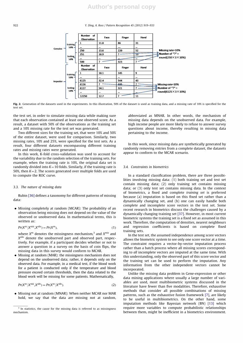
Fig. 2 illustrates the construction of training sets and test setsused in this study. Fifty percent of the score vectors were firstrandomly selected from the dataset as the training set. Theproportion of genuine scores to imposter scores was set to 1:4.The remaining score vectors were used as the test set. Next, foreach modality, 10% of the scores were randomly removed from

0 50 100 150 200 250 3000

0.02

0.04

0.06

0.08

Face Matching Score in the Training Set

Pro

babi

lity

Genuine ScoresImposter ScoresAll Scores

500 1000 15000

0.02

0.04

0.06

0.08

0.1

0.12

0.14

Fingerprint Matching Score in the Training Set

Pro

babi

lity


0 200 400 600 800 10000

0.01

0.02

0.03

0.04

0.05

Hand−Geometry Matching Score in the Training Set

Pro

babi

lity


0 0.2 0.4 0.6 0.8 10

0.2

0.4

0.6

0.8

1

Fusion Score in the Training Set

Pro

babi

lity


Fig. 1. Density plots of the genuine and imposter scores in the raw training set. Here, 50% of the dataset is used as training data. (a) Face, (b) fingerprint, (c) hand-geometry,

(d) after fusion.

Y. Ding, A. Ross / Pattern Recognition 45 (2012) 919–933 921


the test set, in order to simulate missing data while making surethat each observation contained at least one observed score. As aresult, a dataset with 50% of the observations as the training setand a 10% missing rate for the test set was generated.

Two different sizes for the training set, that were 10% and 50%of the entire dataset, were used for comparison. Similarly, twomissing rates, 10% and 25%, were specified for the test sets. As aresult, four different datasets encompassing different trainingrates and missing rates were generated.

In this work, K-fold cross-validation was used to account forthe variability due to the random selection of the training sets. Forexample, when the training rate is 10%, the original data set israndomly divided into K¼10 folds. Similarly, if the training rate is50%, then K¼2. The scores generated over multiple folds are usedto compute the ROC curve.

3.3. The nature of missing data

Rubin [36] defines a taxonomy for different patterns of missingdata:

� Missing completely at random (MCAR): The probability of anobservation being missing does not depend on the value of theobserved or unobserved data. In mathematical terms, this iswritten as:

PrðXm9Xmis,XobsÞ ¼ PrðXmÞ, ð1Þ

where Xm denotes the missingness mechanism,3 and Xmis andXobs denote the unobserved part and observed part, respec-tively. For example, if a participant decides whether or not toanswer a question in a survey on the basis of coin flips, themissing data in this survey would conform to MCAR.� Missing at random (MAR): the missingness mechanism does not

depend on the unobserved data; rather, it depends only on theobserved data. For example, in a medical test, if the blood workfor a patient is conducted only if the temperature and bloodpressure exceed certain thresholds, then the data related to theblood work will be missing for some patients. Mathematically,

PrðXm9Xmis,XobsÞ ¼ PrðXm9XobsÞ: ð2Þ

� Missing not at random (MNAR): When neither MCAR nor MARhold, we say that the data are missing not at random,

abbreviated as MNAR. In other words, the mechanism ofmissing data depends on the unobserved data. For example,high income people are more likely to refuse to answer surveyquestions about income, thereby resulting in missing datapertaining to the income.

In this work, since missing data are synthetically generated byrandomly removing entries from a complete dataset, the datasetsappear to conform to the MCAR scenario.

3.4. Constraints in biometrics

In a standard classification problem, there are three possibi-lities involving missing data: (1) both training set and test setcontain missing data; (2) only training set contains missingdata; or (3) only test set contains missing data. In the contextof biometrics, a fixed and complete training set is preferredbecause (a) imputation is based on this fixed set rather than adynamically changing set, and (b) one can easily handle bothcomplete and incomplete score vectors in the test set. Somerecent research in biometrics discuss the challenges caused by adynamically changing training set [37]. However, in most currentbiometric systems the training set is a fixed set as assumed in thiswork. Therefore, the computation of densities, nearest neighboursand regression coefficients is based on complete fixedtraining sets.

In the test set, the assumed independence among score vectorsallows the biometric system to see only one score vector at a time.The constraint requires a vector-by-vector imputation processrather than a batch process where all missing scores correspond-ing to all incomplete vectors are imputed at the same time. Withthis understanding, only the observed part of this score vector andthe training set can be used to perform the imputation. Anyinformation from the other independent vectors cannot beincorporated.

Unlike the missing data problem in Gene-expression or otherdata mining applications where usually a large number of vari-ables are used, most multibiometric systems discussed in theliterature have fewer than five modalities. Therefore, exhaustivemethods that consider all possible combinations of missingpatterns, such as the exhaustive fusion framework [7], are likelyto be useful in multibiometrics. On the other hand, someimputation methods like Bayesian network (BN) [13] whichrequire more variables to compute probabilistic relationshipsbetween them, might be inefficient in a biometrics environment.

Fig. 2. Generation of the datasets used in the experiments. In this illustration, 50% of the dataset is used as training data, and a missing rate of 10% is specified for the

test set.

3 In statistics, the cause for the missing data is referred to as missingness

mechanism.



3.5. Design of experiments

Table 1 shows seven different imputation schemes discussedin this work, and the related tools or packages used in theexperiments. Table 2 shows the properties of each imputationscheme. Three factors, viz., model assumption, imputation pro-cess and the number of imputations, are considered. Based on thistable, it is difficult to test the interaction between differentfactors, so this work focuses on testing the main effect of eachfactor. Experiments are implemented in four different groupsbased on the property of the schemes:

1. MLE-MN vs. PMM2. GMM-RD vs. GMM-KNN3. PMM vs. KNN vs. GMM-KNN4. MI via MCMC vs. MICE

Receiver operating characteristic (ROC) curves are used toevaluate performance at multiple training set sizes andmissing rates.

3.6. Criteria in biometrics

As stated by Marker et al. [38], two major criteria should beemployed in assessing the performance of imputation methods:firstly, a good imputation method should preserve the naturalrelationship between variables in a multivariate dataset (in ourcase, the variables correspond to scores originating from multiplematchers); secondly, a good imputation method should embodythe uncertainty caused by the imputed data by deriving varianceestimates.

These two criteria are applicable for imputation in a biometricscore dataset. Additionally, the matching accuracy which might

be increased (or decreased) by the imputation is more criticalthan the similarity between the missing values and the imputedvalues in biometrics. So the use of imputed data should result incomparable matching performance to that of the original datacontaining no missing scores.

The min–max normalization scheme followed by the simplesum of scores has been observed to result in reasonable improve-ment in matching accuracy of a multimodal biometric system [2].This scheme was used to generate ROC curves to summarize thefusion results of various imputation methods.

4. Description of imputation methods

4.1. Notation

In the context of multimodal biometric systems, a user i offersp biometric modalities. The system will generate a vector of matchscores, xi ¼ ðxi1,xi2, . . . ,xipÞ, where each match score corresponds toone modality. Suppose that there are n users, then the scorematrix with n observations and p variables can be written as:

D¼

x1

x2

^

xn

0BBB@

1CCCA¼

x11 x12 . . . x1p

x21 x22 . . . x2p

^ ^ xij ^

xn1 xn2 . . . xnp

0BBBB@

1CCCCA,

where xij denotes the match score from the jth modality of the ithuser. Similarly, the training set can be expressed as Dtr.

If there is no missing data, the conventional fusion techniquescan be implemented on each observation (row) separately. Anyobservation xi containing missing scores can be written in theform ðxobs

i ,xmisi Þ, where xobs

i and xmisi , respectively, denote the

observed and missing variables (i.e., scores) for observation i.The missing values xmis

i can be replaced with the imputed valueximp

i using the schemes considered below. For certain schemes, itis more clear to express the p different modalities of the scorematrix as D¼ ðX1,X2, . . . ,XpÞ, and note here that the uppercase X

is used.Different multivariate distributions will be assumed in the

following schemes. Let Y denote all the parameters to beestimated in a particular model. Take the MLE scheme as anexample. The dataset D will be assumed to have a p-variatenormal distribution with mean l¼ ðm1, . . . ,mpÞ and covariancematrix S, so here Y¼ ðl,SÞ corresponds to the parameters of themultivariate normal distribution. Since several schemes useiterative algorithms for estimation, let t denote an iterationcounter, and then YðtÞ denotes all the parameters to be estimatedat the tth iteration.

4.2. K-nearest neighbor imputation

In a classical KNN imputation, the missing values of anobservation are imputed based on a given number of instances(k) in Dtr that are most similar to the instance of interest.

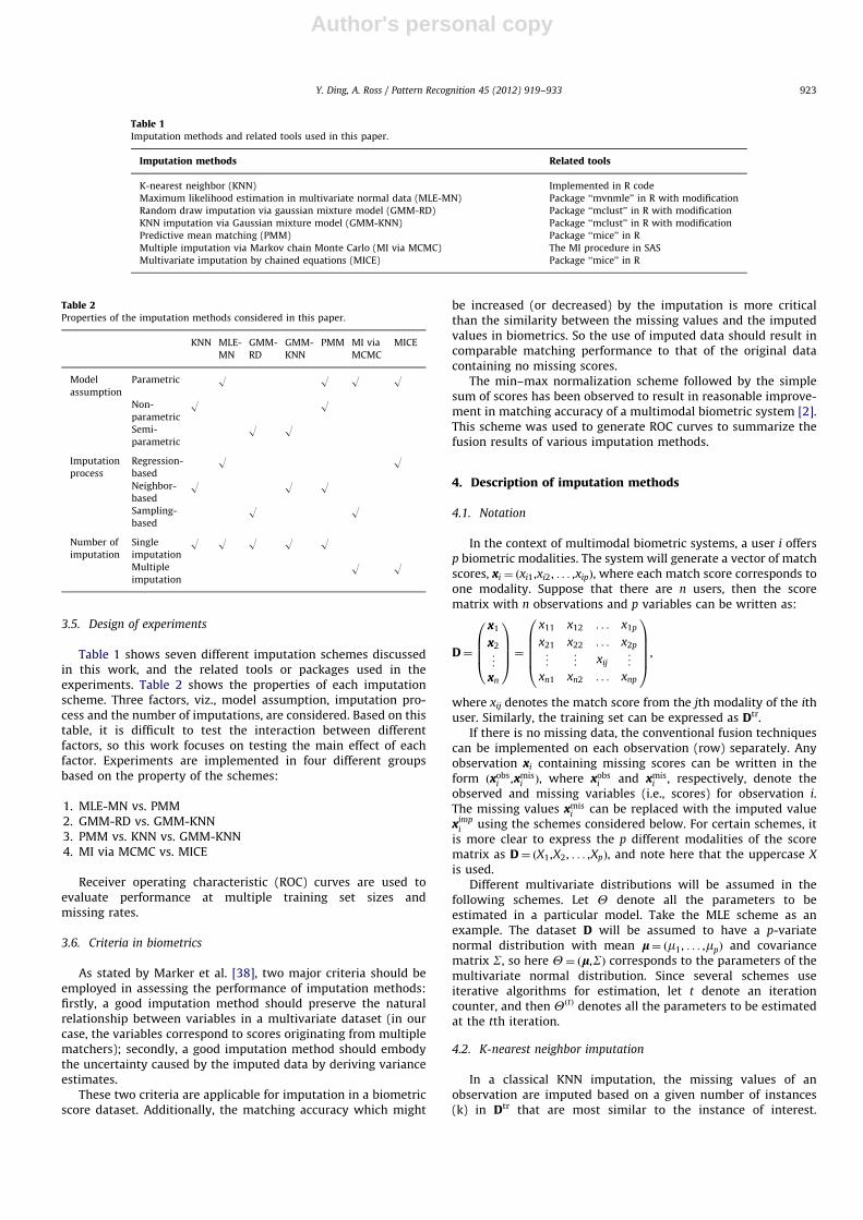
Table 1Imputation methods and related tools used in this paper.

Imputation methods Related tools

K-nearest neighbor (KNN) Implemented in R code

Maximum likelihood estimation in multivariate normal data (MLE-MN) Package ‘‘mvnmle’’ in R with modification

Random draw imputation via gaussian mixture model (GMM-RD) Package ‘‘mclust’’ in R with modification

KNN imputation via Gaussian mixture model (GMM-KNN) Package ‘‘mclust’’ in R with modification

Predictive mean matching (PMM) Package ‘‘mice’’ in R

Multiple imputation via Markov chain Monte Carlo (MI via MCMC) The MI procedure in SAS

Multivariate imputation by chained equations (MICE) Package ‘‘mice’’ in R

Table 2Properties of the imputation methods considered in this paper.

KNN MLE-

MN

GMM-

RD

GMM-

KNN

PMM MI via

MCMC

MICE

Model

assumption

Parametric O O O O

Non-

parametricO O

Semi-

parametricO O

Imputation

process

Regression-

basedO O

Neighbor-

basedO O O

Sampling-

basedO O

Number of

imputation

Single

imputationO O O O O

Multiple

imputationO O



A measure of distance d between two instances should bedetermined. In this work, a Euclidean distance function is con-sidered. Let xi and xj be two observations; then d is defined as:

dðxi,xjÞ ¼X

hAOi\Oj

ðxih�xjhÞ2, ð3Þ

where Oi ¼ fh9the hth variable of the i th observation is observedg.In other words, only the mutually observed variables are used tocalculate the distance between observations.

The KNN algorithm is described as follows:

(1) For each observation xi, apply the distance function d to findthe k nearest neighbor vectors in the training set Dtr;

(2) The missing variables xmisi are imputed by the average of the

corresponding variables from those k nearest neighbors.

KNN imputation does not require the creation of a predictivemodel for each variable, and so it can easily treat instances withmultiple missing values. However, there are some concerns withrespect to KNN imputation. Firstly, which distance functionshould be used for a particular dataset? The choice could beEuclidean, Manhattan, Mahalanobis, Pearson, etc. In this work theEuclidean distance is employed. Secondly, the KNN algorithmsearches through the entire dataset looking for the mostsimilar instances, and can therefore be a very time consumingprocess. Thirdly, the choice of k will impact the results. The choiceof a small k may produce a deterioration in the performance ofthe classifier after imputation due to overemphasis on afew dominant instances in the estimation process of themissing values. On the other hand, a neighborhood of large sizewould include instances that are significantly different fromthe instance containing missing values thereby impacting theestimation process, and the classifier’s performance declines.According to our analysis (not shown here), we found k¼5 toprovide the best imputation accuracy on our relatively smalldataset.

4.3. Imputation via the MLE in multivariate normal data

The imputation scheme using the MLE with a multivariatenormal assumption (MLE-MN) was first described by Dempsteret al. [39] in their influential paper on the EM algorithm. Thekey idea of EM is to solve a difficult incomplete-data estimationproblem by iteratively solving an easier complete-data problem.Intuitively, ‘‘fill’’ in the missing data with the best guess underthe current estimate of the unknown parameters (E-STEP),then re-estimate the parameters from the observed andfilled-in data (M-STEP). An overview of EM has been given in[12,16,40].

In order to obtain the correct answer, Dempster et al. [39]showed that, rather than filling in the missing data values per se,the complete-data sufficient statistics should be computed inevery iteration. The form of these statistics depends on the modelunder consideration. With the assumption of K-variate normaldistribution, the hypothetical complete dataset D belongs to theregular exponential family. So

Pni ¼ 1 xik and

Pni ¼ 1 xikxij are suffi-

cient statistics of samples from this distribution ðj,k¼ 1, . . . ,KÞ.The modified tth iteration of E-STEP can then be written as:

EXn

i ¼ 1

xik9Dtr,xobs

i ,YðtÞ !

¼Xn

i ¼ 1

xðtÞik , k¼ 1, . . . ,K ,

EXn

i ¼ 1

xikxij9Dtr,xobs

i ,YðtÞ !

¼Xn

i ¼ 1

ðxðtÞik xðtÞij þcðtÞijkÞ,

where

xðtÞik ¼xik if xik is observed,

Eðxik9Dtr,xobs

i ,YðtÞÞ if xik is missing,

(

and

cðtÞijk ¼0 if xik or xij is observed,

Covðxik,xij9Dtr,xobs

i ,YðtÞÞ if xik and xij are missing:

(

Missing values xik are thus replaced by the conditional mean ofxik given the set of values xobs

i , available for that observation.These conditional means and the nonzero conditional covariancesare easily found from the current parameter estimates by sweep-ing the augmented covariance matrix so that the variables xobs

i arepredictors in the regression equation and the remaining variablesare outcome variables.

The M-STEP of the EM algorithm is straightforward and is astandard MLE process, i.e.,

mðtþ1Þk ¼

1

n

Xn

i ¼ 1

xðtÞik , k¼ 1, . . . ,K , ð4Þ

sðtþ1Þjk ¼

1

nEXn

i ¼ 1

xikxij9Dtr,xobs

i

!�mðtþ1Þ

k mðtþ1Þj : ð5Þ

The algorithm will iterate repeatedly between the two stepsuntil the difference between covariance matrices in subsequentM-STEPs falls below some specified convergence criterion.Although the classical EM algorithm will stop at this M-STEP, itis straightforward to get the imputed values by performing theE-STEP one more time, using the sweep operator [39] and theregression equations with xobs

i as predictors.

4.4. Imputation via the GMM estimation

As mentioned earlier, the MLE method is based on the multi-variate normal assumption to determine the form of the like-lihood function and sufficient statistics. Although this assumptionis mild, an obvious violation of normality often happens inbiometrics because of the inherent discrimination between gen-uine and imposter scores.

Finite mixture models allow more flexibility, because they arenot constrained to one specific functional form. As shown in Fraleyand Raftery [20], many probability distributions can be wellapproximated by mixture models. At the same time, in contrastto non-parametric schemes, mixture models do not require a largenumber of observations to obtain a good estimate [41,21].

Let observations x1, . . . ,xn be a random sample from a finitemixture model with K underlying components in unknownproportions p1, . . . ,pK . Let the density of xi in the kth componentbe fkðxi; hkÞ, where hk is the parameter vector for component k. Inthis case, Y¼ ðp1, . . . ,pK ; h1, . . . ,hK Þ ¼ ðp,hÞ, and the density of xi

can be written as:

f ðxi;YÞ ¼XK

k ¼ 1

pkfkðxi; hkÞ,

wherePK

k ¼ 1 pk ¼ 1,pkZ0, for k¼1,y,K.Finite mixture models are frequently used when the component

densities fkðxi; hkÞ are taken to be p-variate normal distributionsxi �Npðlk,SkÞ, where the ith observation belongs to component k.This model has been studied by Titterington et al. [42], and byMcLachlan & Basford [43]. Further details on the maximum like-lihood estimates of the components of Y can be found in McLa-chlan and Peel [44].

When Gaussian mixture models are used in imputation, twomain steps will be essential: the density estimation using the



GMM assumption and the imputation itself based on this esti-mated density.

4.4.1. Density estimation using GMM

The EM algorithm of Dempster et al. [39] is applied to thefinite mixture model for density estimation. Let the vector ofindicator variables, zi ¼ ðzi1, . . . ,ziK Þ, be defined by:

zik ¼1 if observation iAcomponent k,

0 if observation i =2 component k:

(

where zi, i¼ 1, . . . ,n, are independently and identically distribu-ted according to a multinomial distribution generated by a singletrial of an experiment with K mutually exclusive outcomes havingprobabilities p1, . . . ,pK .

Let Y denote the maximum likelihood estimate of Y. Then eachobservation, xi, can be allocated to component k on the basis of theestimated posterior probabilities. The estimated posterior prob-ability that observation xi, belongs to component k, is given by:

z ik ¼ prðobservation iAcomponent k9xi; YÞ

¼pkfkðxi; hkÞPK

k ¼ 1 pkfkðxi; hkÞ:

and xi is assigned to component k if:

z ik4 z ik0 for k,k0 ¼ 1, . . . ,K kak0:

The EM algorithm consists of defining an initial guess for theparameters to be estimated, and iteratively estimating the para-meters until convergence of the expectation step (E-step) and themaximization step (M-step).

The E-step requires calculating the expectation of the log-likelihood of the complete data conditioned on the observed dataand the current value of the parameters:

z ik ¼ zðtÞik ¼ Eðzik9x

obsi ;YðtÞÞ ¼

pkfkðxobsi ; hðtÞk ÞPK

k ¼ 1 pkfkðxobsi ; hðtÞk Þ

:

That is, zik is replaced by z ik, the estimate of the posteriorprobability that observation i belongs to component k. With thisestimate z ik, every component of our hypothetical complete datacan be considered as a member of the regular exponential familywith sufficient statistics:

Xn

i ¼ 1

zikxij andXn

i ¼ 1

zikxijxij0 , j,j0 ¼ 1, . . . ,K

So, the remaining calculations in the E-step are analogous to thoserequired in the standard EM algorithm for incomplete normaldata:

Eðzikxij9xobsi ; hðtÞk Þ ¼

z ikxij, xij observed,

z ikEðxij9xobsi ; hðtÞk Þ, xij missing:

(

Eðzikx2ij9x

obsi ; hðtÞk Þ ¼

z ikx2ij, xij observed,

z ik½ðEðxij9xobsi ;hðtÞk ÞÞ

2þVarðxij9xobs

i ; hðtÞk Þ�, xij missing:

8<:

For ja j0,

Eðzikxijxij0 9xobsi ; hðtÞk Þ ¼

z ikxijxij0 , xij and xij0observed,

z ikxijEðxij0 9xobsi ;hðtÞk Þ, xij observed, xij0 missing,

z ikEðxij9xobsi ;hðtÞk Þxij0 , xij0 observed,xij missing,

8>><>>:

In summary, if any value of xi is missing, it will be replaced by theconditional mean of the corresponding variable, given the set ofvalues observed for that observation, xobs

i . When both xij and xij0

are missing, the calculation will be:

Eðzikxijxij0 9xobsi ; hðtÞk Þ ¼ zik½Eðxij9x

obsi ; hðtÞk ÞEðxij0 9x

obsi ; hðtÞk ÞþCorðxij,xij0 9x

obsi ; hðtÞk Þ�:

In the M-step of the algorithm, the new parameters hðtþ1Þ areestimated from the sufficient statistics of the complete data:

pðtþ1Þk ¼

1

n

Xn

i ¼ 1

zðtÞik for k¼ 1, . . . ,K ,

mðtþ1Þkj ¼

1

npkEXn

i ¼ 1

zðtÞik xij9x

obsi ; hðtÞk

!,

Sðtþ1Þ

kjj0 ¼1

npkEXn

i ¼ 1

zðtÞik xijxij0 9x

obsi ; hðtÞk

!�mðtþ1Þ

kj mðtþ1Þkj0 :

Although a mixture model has great flexibility in modeling, arestriction on the number of components K is still requiredbecause, along with an increase in the number of parameters,the estimation of these parameters from the training data mightimply a greater variance for each of the parameters. In this study,the Bayesian information criterion (BIC) [45] is employed. The BICcan be written as

BIC ��2LðY9xobsÞþnK logðntrÞ,

where LðY9xobsÞ is the maximized log-likelihood function giventhe observed data, nK is the number of parameters to be estimatedin the assumed model, and ntr is the number of observations intraining set. The target is to find that nK which minimizes BIC, andthen a reasonable number of components K is obtained.

4.4.2. Two imputation methods via the GMM

With a reasonable density estimation method, various impu-tation schemes are possible. DiZio et al. [21] point out that for thepreservation of the covariance structure, the Random Draw (RD)imputation process based on the GMM assumption (GMM-RD) ispreferable over the conditional mean method (introduced byNielsen [46]) based on the same model.

The estimates of the Gaussian mixture model parameters areobtained as:

f ðxi;YÞ ¼XK

k ¼ 1

pikNpðxi;lk,SkÞ: ð6Þ

In practice, the random drawing of a value xmisi from the

distribution of

f ðxmisi 9xobs

i ;YÞ ¼XK

k ¼ 1

pikNpðxmisi 9xobs

i ;YÞ, ð7Þ

could be accomplished in two simple steps: First, draw a value k

from the multinomial distribution Multið1; p i1, . . . ,p iK Þ; then,given k, generate a random value from the p-variate conditionalGaussian distribution Npðxmis

i 9xobsi ;YÞ as the imputation of the

missing value.The KNN imputation process can also be used based on the

GMM assumption (GMM-KNN). As a neighbor-based method, themain principle of the GMM-KNN method is to find the mostsimilar vectors as ‘‘donors’’ in the training set. However, if thecurrent training set is not large enough, only limited donorswould be available, and this will reduce the accuracy of imputa-tion. In the experiments, a larger simulated dataset ðnsim ¼ 10ntrÞ

based on the estimates of the mixture model parameters is usedas the ‘‘imputation pool’’.

In this work, the Euclidean distance measurement d is employedto find the ‘‘nearest’’ donors for incomplete score vectors. Recall thatthe distance measure d between two observations xi and xj has been



defined in Eq. (3). The GMM-KNN scheme can be summarized in thefollowing steps:

(1) Use the estimated parameters of GMM, Y, to simulate adataset Dsim, having a larger size than Dtr.

(2) For each observation xi, apply the distance function d to findk¼5 nearest neighbors in the simulated set Dsim.

(3) The missing variables xmisi are imputed by the average of

corresponding variables from the nearest neighbors takenfrom Dsim.

4.5. Predictive mean matching (PMM)

Predictive mean matching (PMM) is an imputation schemethat combines some aspects of parametric and non-parametricimputation methods [47]. It imputes missing values by means ofthe neighbor-based schemes, where the distance is computed onthe expected values of the missing variables conditioned on theobserved variables, instead of directly on the values of thevariables. In the PMM scheme, the expected values are computedthrough a linear regression model, such as in the MLE-MN scheme.

(1) The parameters of a multivariate normal distribution areestimated through the EM algorithm [27] using the trainingdata which is complete.

(2) Based on the estimates from EM, for each incomplete scorevector (recipient), predictions of the missing values arecomputed conditioned on the observed variables. These pre-dictions are not directly used as imputation values; rather,they are used to compute the predictive means correspondingto the missing values.

(3) Each recipient is matched to the donor having the closestpredictive mean with respect to the Mahalanobis distance,which is defined through the residual covariance matrix fromthe regression of the missing entries on the observed ones.

(4) Missing values are imputed to each recipient by transferringthe corresponding values from its closest donor.

Although the imputation based on distance function is morerobust than the imputation based on standard linear regression,the asymptotic properties of the neighbor-based methods are nolonger guaranteed, because the measurement of distance used inPMM is not from a non-parametric model but from the results of amultivariate normal model. Thus, if the assumption is not appro-priate, the performance is expected to be poor. Certain improvedPMM methods that use more generalized model assumptionshave been discussed in the literature [48].

4.6. Multiple imputation via MCMC

The primary shortcoming associated with the single imputa-tion schemes discussed earlier – the inability to accommodatevariability/uncertainty – can be attenuated by MI schemes.Proposed by Rubin [27], the MI scheme accounts for missing databy restoring not only the natural variability in the missing data,but by also incorporating the uncertainty caused by the estima-tion process. The general strategies of the MI scheme are asfollows:

(1) Impute missing values using an appropriate model which canplausibly represent the data with random variation.

(2) Repeat this m41 times to produce m completed data sets.(3) Perform the analysis of the complete data.(4) Combine the results of these analysis to obtain overall

estimates using Rubin’s Rules [27].

There are some options for choosing the appropriate model instep (1). The Markov Chain Monte Carlo (MCMC) methods are usedin this work. In statistical applications, MCMC is used to generatepseudo-random samples from multidimensional and otherwiseintractable probability distributions via Markov chains. Data aug-mentation (DA), originated by Tanner and Wong [49], is a veryeffective tool for constructing deterministic models using the MCMCtechnique, when a multivariate normal distribution is assumed.

The DA algorithm starts with the construction of the so-calledaugmented data, xaug

i , which are linked to the observed data via amany-to-one mapping M : xaug

i -xobsi . A data augmentation

scheme is a model for xaugi , pðxaug9yÞ, which satisfies the following

constraint:ZMðxaug

iÞ ¼ xobs

i

pðxaugi 9YÞmðdxaug

i Þ ¼ pðxobsi 9YÞ: ð8Þ

With an appropriate choice of pðxaugi 9YÞ, sampling from

both pðY9xaugi Þ and pðxaug

i 9xobsi ,YÞ is much easier than sampling

directly from pðY9xobsi Þ. Consequently, starting with an initial

value, Yð0Þ, a Markov chain can be formed as ðYðtÞ,xaug,ðtÞÞ,t41by iteratively drawing xaug,ðtþ1Þ

i and Yðtþ1Þ from pðxaugi 9YðtÞ,xobs

i Þ

and pðY9xaug,ðtþ1Þi Þ , respectively.

The two steps are iterated long enough for the results to bereliable for a multiply imputed data set [16]. The goal is to havethe iterations converge to their stationary distribution and then tosimulate an approximately independent draw of the missingvalues.

After obtaining m imputed data sets, the overall estimates arecomputed using Rubin’s Rules [27]: the overall estimate is the simpleaverage of the m estimates, and the overall estimate of the standarderror is a combination of the within-imputation variability, W, andthe between-imputation variability, B:

T ¼Wþ 1þ1

m

� �nB

� �: ð9Þ

4.7. Multivariate imputation by Chained Equations

Multivariate imputation by chained equations (MICE) is anattempt to combine the attractive aspects of two schemes,Regression-based imputation and Multiple imputation. A condi-tional distribution for the missing data corresponding to eachincomplete variable is specified by MICE. For example, thedistribution can be in the form of a linear regression of theincomplete variables given a set of predictors, which can also beincomplete. It is assumed that the joint distribution can befactored into marginal distributions and conditional distributions,and then iterative Gibbs sampling from the conditional distribu-tions can generate samples from the joint distribution.

Recall the score matrix can be written as D¼ ðX1, . . . ,XpÞ,where each variable Xj may be partially observed, withj¼ 1, . . . ,k. The imputation problem requires us to draw fromthe underlying joint distribution of D. Under the assumption thatthe nature of missing data is MAR, one may repeat the followingsequence of Gibbs sampler iterations:

For X1 : draw Xtþ11 from PðX19Xt

2,Xt3, . . . ,Xt

kÞ

For X2 : draw Xtþ12 from PðX29Xtþ1

1 ,Xt3, . . . ,Xt

kÞ

. . .

For Xp : draw Xtþ1p fromPðXp9Xtþ1

2 ,Xtþ13 , . . . ,Xtþ1

p�1 Þ

Rubin and Schafer [25] show that if D is multivariate normal,then iterating linear regression models like X1 ¼ Xt

2b12þXt3b13

þ � � � þXtpb1pþe1 with e1 �Nð0,s2

1Þ will produce a random draw



from the desired distribution. In this way, the multivariateproblem is split into a series of univariate problems.

5. Results and conclusion

5.1. MLE-MN vs. PMM

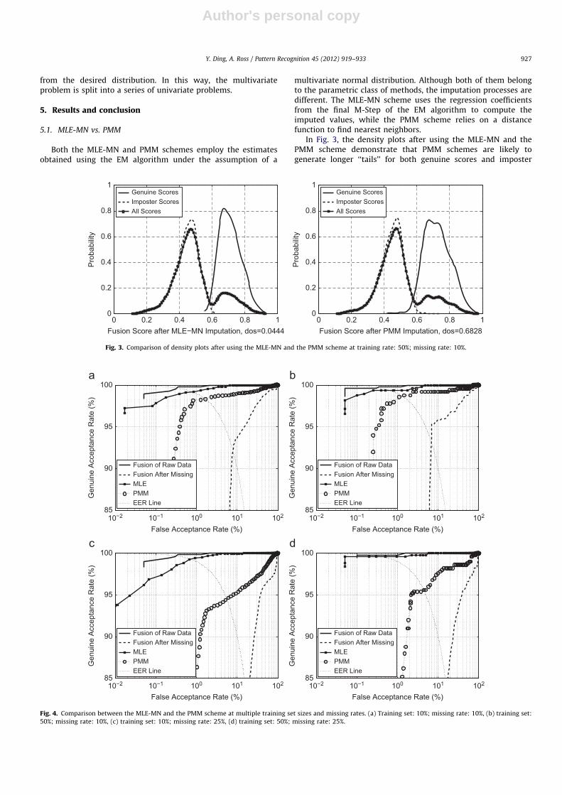
Both the MLE-MN and PMM schemes employ the estimatesobtained using the EM algorithm under the assumption of a

multivariate normal distribution. Although both of them belongto the parametric class of methods, the imputation processes aredifferent. The MLE-MN scheme uses the regression coefficientsfrom the final M-Step of the EM algorithm to compute theimputed values, while the PMM scheme relies on a distancefunction to find nearest neighbors.

In Fig. 3, the density plots after using the MLE-MN and thePMM scheme demonstrate that PMM schemes are likely togenerate longer ‘‘tails’’ for both genuine scores and imposter

0 0.2 0.4 0.6 0.8 10

0.2

0.4

0.6

0.8

1

Fusion Score after MLE−MN Imputation, dos=0.0444

Pro

babi

lity


0 0.2 0.4 0.6 0.8 10

0.2

0.4

0.6

0.8

1

Fusion Score after PMM Imputation, dos=0.6828

Pro

babi

lity


Fig. 3. Comparison of density plots after using the MLE-MN and the PMM scheme at training rate: 50%; missing rate: 10%.

10−2 10−1 100 101 10285

90

95

100

False Acceptance Rate (%)

Gen

uine

Acc

epta

nce

Rat

e (%

)

Fusion of Raw DataFusion After MissingMLEPMMEER Line

85

90

95

100


Gen

uine

Acc

epta

nce

Rat

e (%

)


85

90

95

100


Gen

uine

Acc

epta

nce

Rat

e (%

)


85

90

95

100


Gen

uine

Acc

epta

nce

Rat

e (%

)


10−2 10−1 100 101 102

10−2 10−1 100 101 102 10−2 10−1 100 101 102

Fig. 4. Comparison between the MLE-MN and the PMM scheme at multiple training set sizes and missing rates. (a) Training set: 10%; missing rate: 10%, (b) training set:

50%; missing rate: 10%, (c) training set: 10%; missing rate: 25%, (d) training set: 50%; missing rate: 25%.



scores. So the overlap area between the two classes sharplyincreases leading to a much inferior recognition performance.Here, the degree of separation dos is defined as follows:

dos¼Number of vectors whose scores are within the overlap

Number of all score vectors:

According to the definition, the smaller the dos is, the better theperformance.

A similar observation can be made from the ROC curves inFig. 4. Here, the fusion performance with the original data

(labeled as ‘‘Fusion of Raw Data’’) and after generating themissing data (labeled as "Fusion After Missing") are used asbaselines in the comparison. It is evident that the regression-based method performs better than the neighbor-based methodunder the same density model (multivariate normal). However,the fusion performance after MLE imputation is lower comparedto that of the raw complete dataset. So a multivariate normalitytest was conducted to determine whether the training set (at 50%training rate) conforms to a multivariate normal distribution. TheE-statistic (energy) test was used for this purpose. The p-value

10−2 10−1 100 101 10295

96

97

98

99

100


Gen

uine

Acc

epta

nce

Rat

e (%

)

Fusion of Raw DataFusion After MissingGMMKNNGMMRDEER Line

95

96

97

98

99

100


Gen

uine

Acc

epta

nce

Rat

e (%

)Fusion of Raw DataFusion After MissingGMMKNNGMMRDEER Line

95

96

97

98

99

100


Gen

uine

Acc

epta

nce

Rat

e (%

)


95

96

97

98

99

100


Gen

uine

Acc

epta

nce

Rat

e (%

)


10−2 10−1 100 101 102

10−2 10−1 100 101 102 10−2 10−1 100 101 102

Fig. 5. Comparison between the GMM-RD and the GMM-KNN schemes at multiple training set sizes and missing rates. (a) Training set: 10%; missing rate: 10%, (b) training

set: 50%; missing rate: 10%, (c) training set: 10%; missing rate: 25%, (d) training set: 50%; missing rate: 25%.

0 0.2 0.4 0.6 0.8 10

0.2

0.4

0.6

0.8

1

Fusion Score after GMMRD Imputation, dos=0.0588

Pro

babi

lity


0 0.2 0.4 0.6 0.8 10

0.2

0.4

0.6

0.8

1

Fusion Score after GMMKNN Imputation, dos=0.0032

Pro

babi

lity


Fig. 6. Comparison of density plots after using the GMM-RD and the GMM-KNN schemes with training set: 50%; missing rate: 10%.



indicated that the data were not normally distributed.This violation of normality in the training set results in theobvious decrease in performance when using simple parametricdensity models.

Comparing (c) and (d) in Fig. 4, it can be observed that utilizinga larger size training set can reduce the impact on fusionperformance brought about by an increasing missing rate.

5.2. GMM-RD vs. GMM-KNN

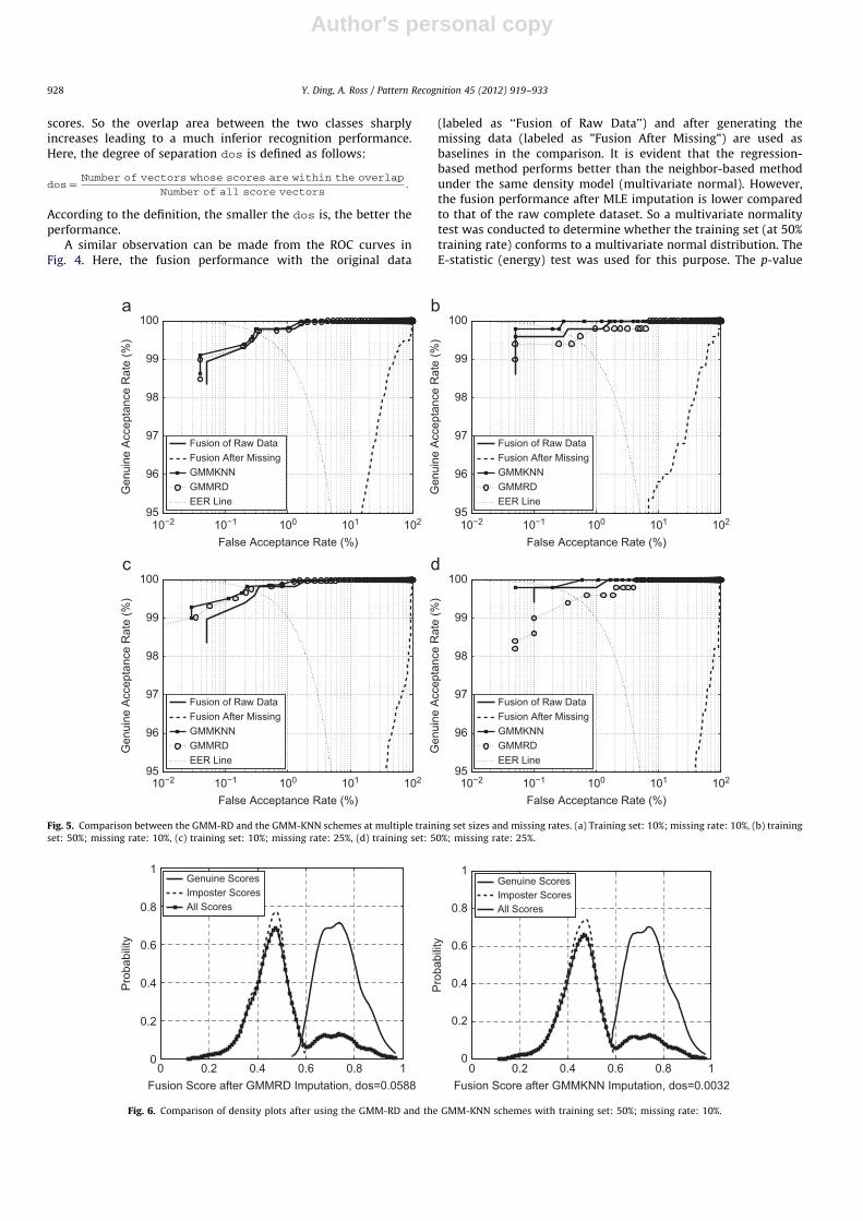
From Fig. 5, both the GMM-RD and GMM-KNN schemes showcomparable performance with that of the raw complete dataset.This can also be observed in Fig. 6. Both schemes have similarlooking density plots since they use the accurate parametersestimated under the GMM assumption.

There is still some subtle differences in the fusion performancedue to the different imputation processes. In Fig. 6, it is observedthat the GMM-KNN imputation scheme results in a decreasedoverlapping area between the two classes. One possible conclu-sion is that a good density model positively impacts the neighbor-based imputation process.

Additionally, GMM-KNN shows consistently better perfor-mance than the sampling-based process, and the differencebecomes more noticeable when the training set is large (in(b) and (d) of Fig. 5). The possible reason has to do with thenuances of the imputation process of random sampling. Recall thevalue k which was drawn from Multið1; p i1, . . . ,p iK Þ, that played acritical role in the process, because the final imputed value

depended upon the component that was chosen. A slightly biasedvalue for k will cause an enormous deviation from the truedistribution corresponding to the missing score. In contrast, theGMM-KNN scheme does not rely on the value k, but uses thedistance corresponding to the observed part to choosethe ‘‘closest’’ neighbors in the simulated data.

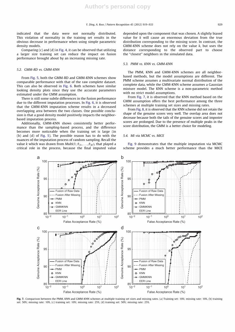
5.3. PMM vs. KNN vs. GMM-KNN

The PMM, KNN and GMM-KNN schemes are all neighbor-based methods, but the model assumptions are different. ThePMM scheme assumes a multivariate normal distribution of thecomplete data, while the GMM-KNN scheme assumes a Gaussianmixture model. The KNN scheme is a non-parametric methodwith no strict model assumptions.

From Fig. 7, it is observed that the KNN method based on theGMM assumption offers the best performance among the threeschemes at multiple training set sizes and missing rates.

From Fig. 8, it is observed that the KNN scheme did not retain theshape of the genuine scores very well. The overlap area does notdecrease because both the tails of the genuine scores and imposterscores are prolonged. Due to the presence of multiple peaks in thescore distribution, the GMM is a better choice for modeling.

5.4. MI via MCMC vs. MICE

Fig. 9 demonstrates that the multiple imputation via MCMCscheme provides a much better performance than the MICE

10−2 10−1 100 101 10285

90

95

100


Gen

uine

Acc

epta

nce

Rat

e (%

)

Fusion of Raw DataFusion After MissingPMMKNNGMMKNNEER Line

85

90

95

100


Gen

uine

Acc

epta

nce

Rat

e (%

)


85

90

95

100


Gen

uine

Acc

epta

nce

Rat

e (%

)


85

90

95

100


Gen

uine

Acc

epta

nce

Rat

e (%

)


10−2 10−1 100 101 102

10−2 10−1 100 101 10210−2 10−1 100 101 102

Fig. 7. Comparison between the PMM, KNN and GMM-KNN schemes at multiple training set sizes and missing rates. (a) Training set: 10%; missing rate: 10%, (b) training




scheme, even when the missing rate is high in (d). From Fig. 10,it is observed that the density plots after applying the MIvia MCMC scheme has a very similar shape as that of the rawtest set.

The squared residuals between the original fusion scores (thesample) and imputed scores (the estimated values) are computedfor the MI via MCMC scheme and the GMM-KNN scheme. Thesum of squared residuals of the MI via MCMC is less than that of

the GMM-KNN. This indicates that the imputed scores from theMI via MCMC scheme are closer to the missing scores. However,the overall recognition accuracy is more critical than the similar-ity between the missing values and the imputed values. Both ROCcurves and dos values indicate that a better recognition perfor-mance is offered by the GMM-KNN scheme.

Both MICE and MLE-MN schemes employ the parametricmodel combined with regression-based imputation, and cannot

10−2 10−1 100 101 10285

90

95

100


Gen

uine

Acc

epta

nce

Rat

e (%

)

Fusion of Raw DataFusion After MissingMI via MCMCMICEEER Line

85

90

95

100


Gen

uine

Acc

epta

nce

Rat

e (%

)


85

90

95

100


Gen

uine

Acc

epta

nce

Rat

e (%

)


85

90

95

100


Gen

uine

Acc

epta

nce

Rat

e (%

)


10−2 10−1 100 101 102

10−2 10−1 100 101 10210−2 10−1 100 101 102

Fig. 9. Comparison between the MI via MCMC and the MICE schemes at multiple training set sizes and missing rates. (a) Training set: 10%; missing rate: 10%, (b) training


0 0.2 0.4 0.6 0.8 10

0.2

0.4

0.6

0.8

1

Fusion Score after KNN Imputation, dos=0.1052

Pro

babi

lity


0 0.2 0.4 0.6 0.8 10

0.2

0.4

0.6

0.8

1

Fusion Score of Raw Test Set, dos=0.0128

Pro

babi

lity


Fig. 8. Comparison of density plots between the raw test set and the imputation set after using the KNN scheme at training set: 50%; missing rate: 10%.



yield a good imputed value while retaining the classificationaccuracy. The MICE, which averages the multiple imputed valuestogether, is observed to result in the worst performance. This is

because the averaging process can only reduce the variance ofestimation, but cannot reduce the bias.

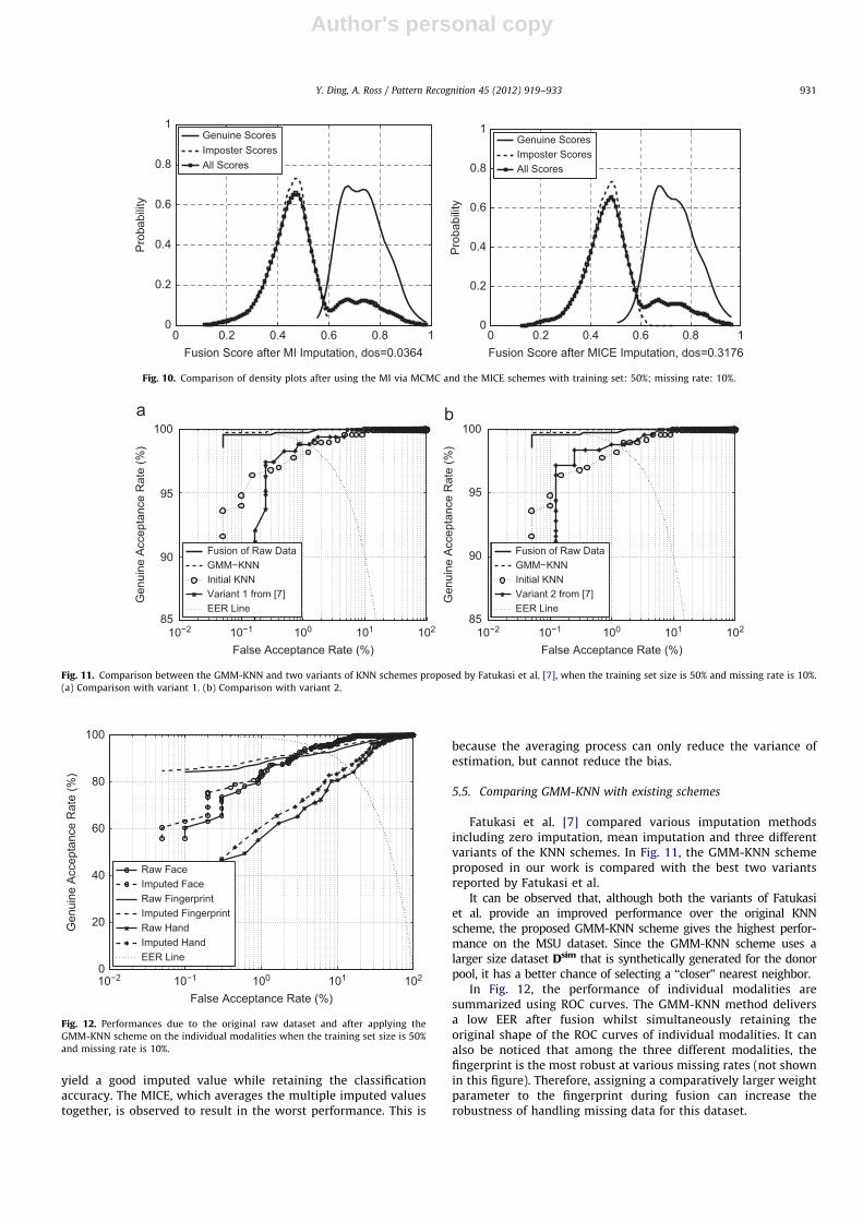
5.5. Comparing GMM-KNN with existing schemes

Fatukasi et al. [7] compared various imputation methodsincluding zero imputation, mean imputation and three differentvariants of the KNN schemes. In Fig. 11, the GMM-KNN schemeproposed in our work is compared with the best two variantsreported by Fatukasi et al.

It can be observed that, although both the variants of Fatukasiet al. provide an improved performance over the original KNNscheme, the proposed GMM-KNN scheme gives the highest perfor-mance on the MSU dataset. Since the GMM-KNN scheme uses alarger size dataset Dsim that is synthetically generated for the donorpool, it has a better chance of selecting a ‘‘closer’’ nearest neighbor.

In Fig. 12, the performance of individual modalities aresummarized using ROC curves. The GMM-KNN method deliversa low EER after fusion whilst simultaneously retaining theoriginal shape of the ROC curves of individual modalities. It canalso be noticed that among the three different modalities, thefingerprint is the most robust at various missing rates (not shownin this figure). Therefore, assigning a comparatively larger weightparameter to the fingerprint during fusion can increase therobustness of handling missing data for this dataset.

0 0.2 0.4 0.6 0.8 10

0.2

0.4

0.6

0.8

1

Fusion Score after MI Imputation, dos=0.0364

Pro

babi

lity


0 0.2 0.4 0.6 0.8 10

0.2

0.4

0.6

0.8

1

Fusion Score after MICE Imputation, dos=0.3176

Pro

babi

lity


Fig. 10. Comparison of density plots after using the MI via MCMC and the MICE schemes with training set: 50%; missing rate: 10%.

10−2 10−1 100 101 10285

90

95

100


Gen

uine

Acc

epta

nce

Rat

e (%

)

Fusion of Raw DataGMM−KNNInitial KNNVariant 1 from [7]EER Line

10−2 10−1 100 101 10285

90

95

100


Gen

uine

Acc

epta

nce

Rat

e (%

)

Fusion of Raw DataGMM−KNNInitial KNNVariant 2 from [7]EER Line

Fig. 11. Comparison between the GMM-KNN and two variants of KNN schemes proposed by Fatukasi et al. [7], when the training set size is 50% and missing rate is 10%.

(a) Comparison with variant 1. (b) Comparison with variant 2.

10−2 10−1 100 101 1020

20

40

60

80

100


Gen

uine

Acc

epta

nce

Rat

e (%

)

Raw FaceImputed FaceRaw FingerprintImputed FingerprintRaw HandImputed HandEER Line

Fig. 12. Performances due to the original raw dataset and after applying the

GMM-KNN scheme on the individual modalities when the training set size is 50%

and missing rate is 10%.



6. Summary

The results in the previous sections indicate that there are certainpowerful imputation schemes, which can sustain the fusion perfor-mance at a high level when the missing rates are small. Specifically,the GMM-based scheme performs better than the other models,because it seems to capture the natural structure of the raw dataset.Further, under the GMM assumption, the non-parametric imputa-tion process is preferred over sampling-based schemes. The experi-ments also indicate that utilizing a larger training set can mitigatethe negative impact on performance at higher missing rates. On theother hand, there are some imputation schemes whose performanceis not comparable to that of the raw (original) dataset; in fact a fewof them such as PMM result in worse fusion performance than thatof a single modality.

In the future, the robustness of the assumptions made forevery scheme will be further analyzed. This is expected to offeradditional guidance on how to choose appropriate imputationmethods for a particular dataset. Also, we are looking at ways tocombine the process of imputation with score normalization andfusion. Finally, these experiments will be repeated on largeoperational data sets using different fusion rules.

Acknowledgments

This work was supported by the NSF Center for IdentificationTechnology Research (CITeR). The authors would like to thank Dr.Anil Jain at Michigan State University for granting us access totheir database. Thanks to the reviewers for their valuable com-ments which significantly improved the experimental analysis.

References

[1] A.K. Jain, P. Flynn, A.A. Ross, Handbook of Biometrics, Springer, 2008.[2] A. Jain, K. Nandakumar, A. Ross, Score normalization in multimodal biometric

systems, Pattern Recognition 38 (12) (2005) 2270–2285.[3] A.A. Ross, K. Nandakumar, A.K. Jain, Handbook of Multibiometrics, Springer,

Secaucus, NJ, USA, 2006.[4] G. King, J. Honaker, A. Joseph, K. Scheve, Analyzing incomplete political

science data: an alternative algorithm for multiple imputation, AmericanPolitical Science Review 95 (2001) 49–69.

[5] R. Brown, Efficacy of the indirect approach for estimating structural equationmodels with missing data: a comparison of five methods, Structural EquationModeling 1 (1994) 287–316.

[6] J. Graham, S. Hofer, D. MacKinnon, Maximizing the usefulness of dataobtained with planned missing value patterns: an application of maximumlikelihood procedures, Multivariate Behavioral Research 31 (1996) 197–218.

[7] O. Fatukasi, J. Kittler, N. Poh, Estimation of missing values in multimodalbiometric fusion, in: IEEE International Conference on Biometrics: Theory,Applications and Systems (BTAS), 2008.

[8] J. Quinlan, Induction of decision trees, Machine Learning 1 (1986) 81–106.[9] O.O. Lobo, M. Noneao, Ordered estimation of missing values for propositional

learning, Journal of the Japanese Society for Artificial Intelligence 1 (2000)499–503.

[10] H.F. Friedman, R. Kohavi, Y. Yun, Lazy decision trees, in: The 13th NationalConference on Artificial Intelligence, 1996, pp. 717–724.

[11] J. Schafer, J. Graham, Missing data: our view of the state of the art,Psychological Methods.

[12] R.J.A. Little, D.B. Rubin, Statistical Analysis with Missing Data, first ed., Wiley,New York, 1987.

[13] N. Friedman, D. Geiger, M. Goldszmidt, Bayesian network classifiers, MachineLearning 29 (2–3) (1997) 131–163.

[14] S.F. Buck, A method of estimation of missing values in multivariate datasuitable for use with an electronic computer, Journal of the Royal StatisticalSociety 22 (2) (1960) 302–306.

[15] R.J.A. Little, Regression with missing x’s: a review, Journal of the AmericanStatistical Association 87 (420) (1992) 1227–1237.

[16] J. Schafer, Analysis of incomplete multivariate data, Chapman & Hall/CRC,London, 1997.

[17] J.K. Dixon, Pattern recognition with partly missing data, IEEE Transactions onSystems, Man and Cybernetics 9 (10) (1979) 617–621.

[18] G. Kalton, D. Kasprzyk, The treatment of missing survey data, SurveyMethodology 1 (12) (1986) 1–16.

[19] M. Bramer, R. Ellis, M. Petridis, A kernel extension to handle missing data,Research and Development in Intelligent Systems 26 (2009) 165–178.

[20] C. Fraley, A. Raftery, Model-based clustering, discriminant analysis, anddensity estimation, Journal of the American Statistical Association 97(2002) 611–631.

[21] M. Di Zio, U. Guarnera, O. Luzi, Imputation through finite gaussian mixturemodels, Computational Statistics and Data Analysis 51 (11) (2007)5305–5316.

[22] J.Q. Li, A.R. Barron, Mixture density estimation, Advances in Neural Informa-tion Processing Systems, vol. 12, MIT Press, 1999, pp. 279–285.

[23] B. Stef Van, O. Karin (CGM), Multivariate Imputation by Chained Equations.MICE V1.0 User’s manual, Vol. PG/VGZ/00.038., TNO Prevention and Health,Leiden, 2000.

[24] T.E. Raghunathan, J.M. Lepkowski, J.V. Hoewyk, P. Solenberger, A multivariatetechnique for multiply imputing missing values using a sequence of regres-sion models, Survey Methodology 27 (2001) 85–95.

[25] D. Rubin, J. Schafer, Efficiently creating multiple imputations for incompletemultivariate normal data, Proceedings of the Statistical Computing Section(1990) 83–88.

[26] D.B. Rubin, N. Schenker, Multiple imputation for interval estimation fromsimple random samples with ignorable nonresponse, Journal of the AmericanStatistical Association 81 (1986) 366–374.

[27] D.B. Rubin, Multiple imputation for nonresponse in surveys, Wiley, 1987.[28] J. Schafer, J. Schenker, Inference with imputed conditional means, Journal of

the American Statistical Association 95 (2000) 144–154.[29] M. Ramoni, P. Sebastiani, Robust learning with missing data, Machine

Learning 45 (2) (2001) 147–170.[30] K. Nandakumar, A.K. Jain, A. Ross, Fusion in multibiometric identification

systems: what about the missing data?, in: IEEE/IAPR International Con-ference on Biometrics, Springer, 2009, pp. 743–752.

[31] N. Poh, D. Windridge, V. Mottl, A. Tatarchuk, A. Eliseyev, Addressing missingvalues in kernel-based multimodal biometric fusion using neutral pointsubstitution, IEEE Transactions on Information Forensics and Security 5 (3)(2010) 461–469.

[32] Y. Ding, A. Ross, When data goes missing: methods for missing scoreimputation in biometric fusion, in: Proceedings of SPIE Conference onBiometric Technology for Human Identification VII, vol. 7667, 2010.

[33] A. Ross, A. Jain, Information fusion in biometrics, Pattern Recognition 13(2003) 2115–2125.

[34] E. Byon, A. Shrivastava, Y. Ding, A classification procedure for highlyimbalanced class sizes, IIE Transactions 4 (42) (2010) 288–303.

[35] S. Oba, M. Sato, I. Takemasa, M. Monden, K. Matsubara, S. Ishii, A bayesianmissing value estimation method for gene expression profile data, Bioinfor-matics 19 (16) (2003) 2088–2096.

[36] D. Rubin, Inference and missing data, Biometrika 63 (1976) 581–592.[37] R. Singh, M. Vatsa, A. Ross, A. Noore, Online learning in biometrics: a case

study in face classifier update, in: IEEE 3rd International Conference onBiometrics: Theory, Applications, and Systems, 2009. BTAS ’09, 2009, pp. 1–6.

[38] D.A. Marker, D.R. Judkins, M. Winglee, Large-scale imputation for complexsurveys, in: Survey Nonresponse, John Wiley and Sons, 1999.

[39] A. Dempster, N. Laird, D. Rubin, Maximum likelihood from incomplete datavia the em algorithm, Journal of the Royal Statistical Society. Series B(Methodological) 1 (39) (1977) 1–38.

[40] G. McLachlan, T. Krishnan, The EM algorithm and extensions, WileyNew York, 1996.

[41] C. Priebe, Adaptive mixtures, Journal of the American Statistical Association89 (1994) 796–806.

[42] D. Titterington, A. Smith, U. Makov, Statistical Analysis of Finite MixtureDistributions, Wiley, New York, 1985.

[43] G. McLachlan, K. Basford, Mixture models: inference and applications toclustering, Marcel-Dekker, New York, 1988.

[44] G. McLachlan, D. Peel, Finite Mixture Models, Wiley, New York, 2000.[45] G. Schwarz, Estimating the dimension of a model, The Annals of Statistics 6

(2) (1978) 461–464.[46] S. Nielsen, Nonparametric conditional mean imputation, Journal of Statistical

Planning and Inference 99 (2001) 129–150.[47] R. Little, Missing data adjustments in large surveys, Journal of Business and

Economic Statistics 6 (3) (1988) 287–296.[48] G. Durrant, C. Skinner, Missing data methods to correct for measurement

error in a distribution function, Survey Methodology 32 (1) (2006) 25–36.[49] M. Tanner, W. Wong, The calculation of posterior distributions by data

augmentatio, Journal of the American Statistical Association 82 (398) (1987)528–540.

Yaohui Ding received the B.S. degree in Electrical Engineering from Zhejiang University, China, in August 2003. He received the M.S. degree in Statistics from West VirginiaUniversity, USA, in August 2010. He is currently pursuing the Ph.D. degree in the Lane Department of Computer Science and Electrical Engineering at West VirginiaUniversity. His current research interest is biometrics fusion.



Arun Ross received the B.E. (Hons.) degree in Computer Science from the Birla Institute of Technology and Science, Pilani, India, in 1996, and the M.S. and Ph.D. degrees inComputer Science and Engineering from Michigan State University, East Lansing, in 1999 and 2003, respectively. Between 1996 and 1997, he was with the Design andDevelopment Group of Tata Elxsi (India) Ltd., Bangalore, India. He also spent three summers (2000–2002) with the Imaging and Visualization Group of Siemens CorporateResearch, Inc., Princeton, NJ, working on fingerprint recognition algorithms. He is currently a Robert C. Byrd Associate Professor in the Lane Department of ComputerScience and Electrical Engineering, West Virginia University, Morgantown. His research interests include pattern recognition, classifier fusion, machine learning, computervision, and biometrics. He is actively involved in the development of biometrics and pattern recognition curricula at West Virginia University. He is the coauthor ofHandbook of Multibiometrics and co-editor of Handbook of Biometrics. Arun is a recipient of NSF’s CAREER Award and was designated a Kavli Frontier Fellow by theNational Academy of Sciences in 2006. He is an Associate Editor of the IEEE Transactions on Image Processing and the IEEE Transactions on Information Forensics andSecurity.


Documents

Author's personal copy - Michigan State Universityrossarun/pubs/DingRossMissing...Author's personal copy process of growing a decision tree is computationally expensive, and requires