AUSTRALIAN BANKING EFFICIENCY AND ITS

RELATION TO STOCK RETURNS*

Joshua Kirkwood & Daehoon Nahm# dnahm@efs.mq.edu.au

ABSTRACT

This paper considers cost and profit efficiency for Australian banks between 1995 and 2002. Data Envelopment Analysis (DEA) is used to construct an efficient frontier for ten banks listed on the Australian Stock Exchange. Empirical results indicate the major banks have improved their cost and profit efficiency, while the regional banks have experienced little change in cost efficiency, and a decline in profit efficiency. This result provides interesting insights into the structure of the Australian banking industry. Malmquist indices indicate technological change is the dominant source of improvements in total factor productivity over the period. An attempt is made to relate the changes in efficiency to stock returns, using a method superior to that previously adopted. Results indicate that for our sample changes in firm efficiency are reflected in stock returns.

JEL Classification: G14, G21, D24

Keywords: DEA, Banks, Profit Efficiency, Cost Efficiency

__________________________________________________________________________________ * This paper is a modified and extended version of a thesis prepared by Joshua Kirkwood during his 2003 honours year at

Macquarie University. Professor Johannes Jütter was also a supervisor during the honours year. # Department of Economics, Macquarie University, Sydney, Australia Tel) +612 9850 9615, Fax) +612 9850 8586, email) dnahm@efs.mq.edu.au

2

1. Introduction

An examination of bank efficiency is important for several reasons. Financial markets in

Australia have undergone significant change over the last decade, as a result of deregulation and

globalisation. These drivers of change were particularly strong over the latter half of the 1990s, which

may be characterised as a period of relatively low interest rates and a period where banks moved away

from simply being intermediaries toward providing a range of financial services – from insurance to

funds management. All of these factors have had a significant influence on the operations of Australian

banks. Because the Australian banking system is dominated by four banks (the major banks), it is

interesting to contrast the performance of these banks to their much smaller counterparts (the regional

banks), who are much less diversified.

This paper makes several contributions. It is the first study of Australian bank efficiency to

consider profit efficiency. Second, the selection of inputs and outputs for the two estimated models is

unique. Third, no study of Australian banking efficiency has estimated Malmquist productivity indices

over the latter part of the 1990s. Finally, an understudied, but important, issue is whether changes in a

firm's efficiency are reflected in stock prices. We assess the relationship between changes in profit

efficiency and stock returns using a method which appears to be superior to that previously adopted.

Data Envelopment Analysis (DEA) is used to estimate cost and profit efficiency and Malmquist

productivity indices are used to separate technological change from changes in efficiency. The analysis

is conducted between 1995 and 2002 for ten banks listed on the Australian Stock Exchange.

DEA is a linear programming technique that estimates an efficient frontier based on the

observations in the sample. Those observations found to be most efficient (and hence are located on

the constructed frontier) are assigned a ‘score’ of 1, while the other observations in the sample are

allocated a score less than one. Input oriented DEA has been used for both of our models, and therefore

an efficiency score of say 0.80 can be interpreted as meaning this bank could reduce inputs by 25 per

cent [(1-0.80)/0.80] without changing output levels. Cost (and profit) efficiency scores are the product

of allocative and technical components, which are also rated on a 0 to 1 scale.

The empirical results indicate that the cost and profit efficiency of the major banks has

improved over the period. For the regional banks, however, there has been little change in cost

efficiency and a deterioration of profit efficiency. We also find that changes in firm efficiency are

reflected in stock prices, but that the magnitude of the relationship is not uniform.

3

The paper is organised as follows: Section 2 reviews the relevant Australian literature; Section

3 introduces the models and empirical results; and Section 4 outlines the model relating changes in

profit efficiency to stock returns and discusses the empirical results.

2. Literature Review

The Australian banking industry is highly concentrated, and may be considered an oligopoly.

The industry is composed of four large banks which account for 68 per cent of total banking assets and

32 per cent of the assets of all Australian financial institutions.1 These large banks, the majors, are

highly diversified, both geographically, and in their sources of income. There are a number of smaller

banks, the regional banks, as well as a number of foreign banks.

Avkiran in a series of papers (1999a, 1999b and 2000) uses DEA to analyse the efficiency of

ten Australian banks in the period following deregulation of the financial sector (1986-1995). Avkiran

(1999b) finds that the dominant source of inefficiency is technical inefficiency (as opposed to scale

inefficiency), and that following deregulation technical efficiency, as well as overall efficiency,

declined between 1986 and 1991, and rose thereafter. The explanations for the decline in efficiency in

the early period of the study include the unprofitable lending decisions of the late 1980s and a

reluctance to raise fees in the face of new competition following deregulation. Despite these

‘aggregate’ results Avkiran (1999b) finds that ‘there is no clear trend for the change in productivity in

the period 1986-1995 that is shared by all the banks’ (p16).

Avkiran (1999b) finds the major banks have operated under decreasing returns to scale, while

the regional banks have operated under increasing returns to scale. We may be sceptical of these

results, however, due to the broad grouping of inputs and outputs (given in Table 1). A study that

separated inputs into labour, physical capital and deposits (the conventional inputs in the literature)

may produce different results because the different types of capital (human, physical and financial)

used in production have been better accounted for.

One of the major limitations of Avkiran (1999b) is ‘the absence of an attempt to analyse the

potential frontier shift from one year to the next,’ possibly due to technological change. This is the

subject of Avkiran (2000), which examines changes in the productivity of retail banking using DEA

calculated Malmquist productivity indices (MPI). The sample characteristics are the same as Avkiran

(1999b).

1 Statistics at March 2002.

4

Over the period 1986 to 1995 Avkiran (2000) finds technical change improved annually by

2.8 per cent, on average; however, technical efficiency increased by 0.7 per cent, on average, per year.

When comparing the regional banks and the major banks, Avkiran (2000) finds that the technical

efficiency scores are much the same for these groups of banks, but with slightly higher variability

amongst regional banks. The major banks, however, exhibited slightly higher rates of technological

progress. Again we ought to be sceptical of Avkiran (2000) results for he uses the same inputs and

outputs as for Avkiran (1999b) – see the critique above. Moreover, Avkiran (2000) assumes constant

returns to scale when using DEA, and as such the results may be biased due to the omission of scale

economies in the model design.

Avkiran (1999a) uses two models to study X-efficiencies (that is, technical and allocative

efficiencies) between 1986 and 1995. The sample size here varies between 16 and 19 banks, which is

larger than the Avkiran (1999b) and Avkiran (2000) studies.

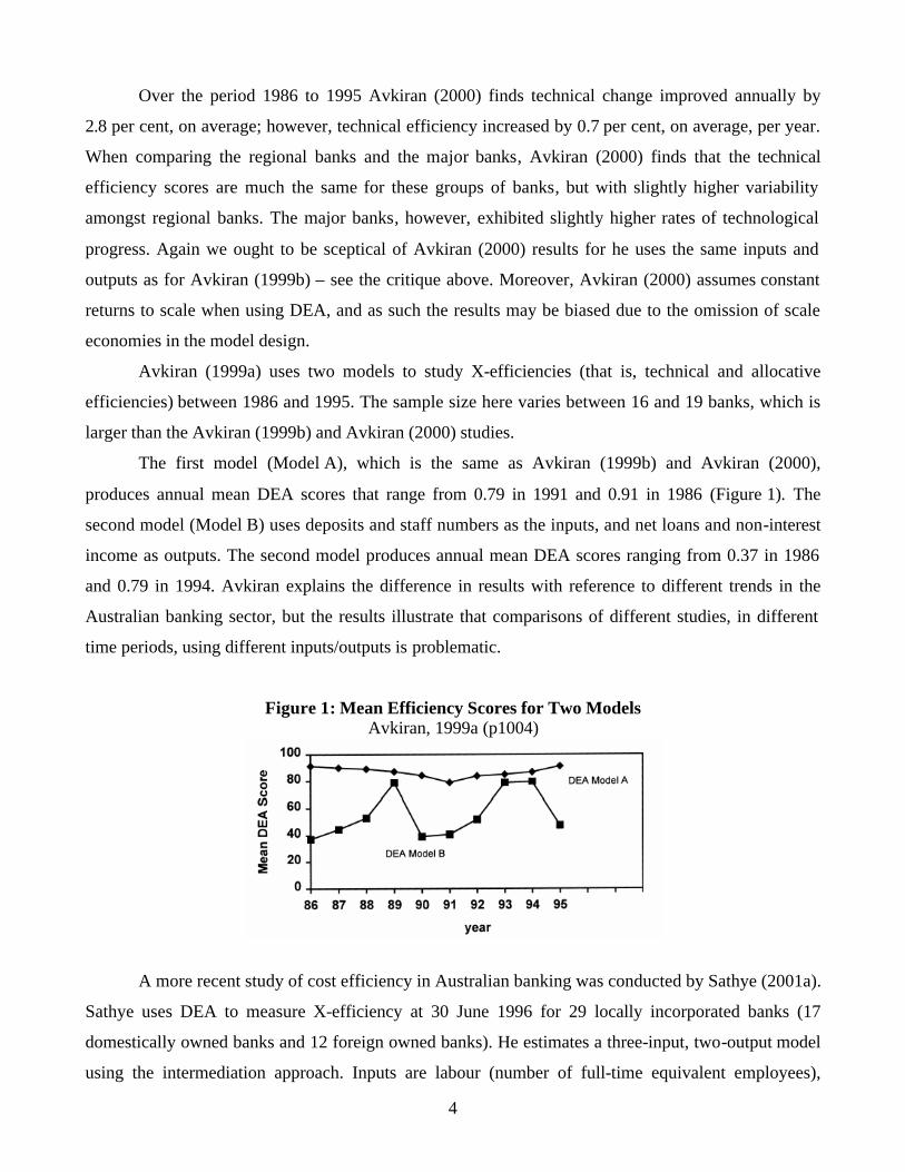
The first model (Model A), which is the same as Avkiran (1999b) and Avkiran (2000),

produces annual mean DEA scores that range from 0.79 in 1991 and 0.91 in 1986 (Figure 1). The

second model (Model B) uses deposits and staff numbers as the inputs, and net loans and non-interest

income as outputs. The second model produces annual mean DEA scores ranging from 0.37 in 1986

and 0.79 in 1994. Avkiran explains the difference in results with reference to different trends in the

Australian banking sector, but the results illustrate that comparisons of different studies, in different

time periods, using different inputs/outputs is problematic.

Figure 1: Mean Efficiency Scores for Two Models Avkiran, 1999a (p1004)

A more recent study of cost efficiency in Australian banking was conducted by Sathye (2001a).

Sathye uses DEA to measure X-efficiency at 30 June 1996 for 29 locally incorporated banks (17

domestically owned banks and 12 foreign owned banks). He estimates a three-input, two-output model

using the intermediation approach. Inputs are labour (number of full-time equivalent employees),

5

physical capital (book value of premises and fixed assets, net of depreciation) and loanable funds (time

deposits, savings deposits and other borrowed funds) whilst outputs are loans and demand deposits.

There are at least two shortfalls of this study. First, it excludes off-balance sheet items as an

output, and second, constant returns to scale are assumed for the DEA model. Both of these factors

may partly account for the low efficiency scores obtained.

Sathye's average Australian efficiency score is 0.58, which is lower than the world average of

0.86 (from Berger and Humphrey’s (1997) international literature review).2 Of this overall efficiency

estimate technical efficiency was found to be very low, while allocative efficiency was fairly high by

world standards. Sathye’s study occurred before the widespread use of electronic banking, which may

go some way toward improving technical efficiency. Further, Sathye notes that in the years following

his study there were large redundancies in several banking institutions.

Sathye also investigates the ownership issue by performing separate DEA estimations (using

the model outlined above) for domestic and foreign banks incorporated in Australia. Domestic banks

have better overall efficiency scores (0.83) than foreign banks (0.62); however, this difference is not

statistically significant, possibly due to the small sample size.

Sturm and Williams (2002) present a comprehensive analysis of Australian banking efficiency

in the post-deregulation period (1988-2001). The sample includes domestic and foreign banks – up to

26 banks in total.3 They develop four models, two of which are presented in Table 1. The first model is

fairly standard, but substitutes equity capital for physical capital. The second model is subject to the

same criticisms of Avkiran (1999a).

In contrast to many studies of banking efficiency overseas (particularly the US) Sturm and

Williams find that scale effects are the main source of inefficiency; but that this dominance is not

strong (some of their models estimated indicate technical efficiency outweigh scale inefficiency). The

four major banks had ‘consistently lower scale efficiency [but]… also had consistently higher pure

technical efficiency’ (p16). Foreign banks displayed superior scale efficiency and, in contrast with

Sathye (2001a), were more efficient overall.

Data availability only allowed Sturm and Williams (2002) to compute Malmquist indices

between 1989 and 1995. They find that technical change was high in 1989/90 and regressed in 1992/3,

largely due to the recession of that period. Finally, they find that ‘the main source of efficiency gains

post-deregulation was technological change rather than technical efficiency’ (p27).

2 Strictly such a comparison should not be made since the efficient frontiers may differ between countries. 3 The sample is an unbalanced panel and the number of banks range from 10 (2001) to 26 (1991).

6

The results of these Australian studies cited are summarised in Table 1. Most of the studies

surveyed have some major drawbacks – some have assumed constant returns to scale, while others

have not adequately specified inputs and outputs (for example off-balance sheet items have been

excluded). As such drawing conclusions is difficult, evidenced by the range of efficiency scores in

Table 1.

A large gap in this literature is the absence of studies that have considered profit efficiency. We

assess profit efficiency using a model similar to Chu and Lim (1998). These authors studied cost and

profit efficiency of the Singaporean banking industry by specifying profit as the output of the DEA

model, rather than specifying the outputs as physical quantities. That is, the question under

consideration is how well the firm converts its inputs into profit.

Chu and Lim (1998) estimated two models – one for profit efficiency and one for cost

efficiency. The model which assesses cost efficiency specifies shareholders’ funds, interest expenses

and operating expenses as inputs, and the annual increase in average assets and total income as outputs.

The model which assesses profit efficiency specifies the same inputs, but uses profit as the output.

The study included six banks which ‘command some 70 per cent of the markets for deposits

and loans’ (p156) between 1992 and 1996. Chu and Lim (1998) found cost efficiencies to be quite high

by international comparisons – 0.95 on average, while profit efficiencies were lower at 0.83. These

findings are consistent with much of the banking efficiency literature, which finds profit inefficiencies

dominate cost inefficiencies (Berger and Humphrey, 1997).

Although most studies of banking efficiency only consider input (cost) inefficiency the

conclusion from Chu and Lim (1998) and other studies is clear. When undertaking a study of firm

efficiency it is essential to consider both input and output inefficiencies. To consider only one will not

yield an accurate assessment of the state of inefficiency in a market.

7

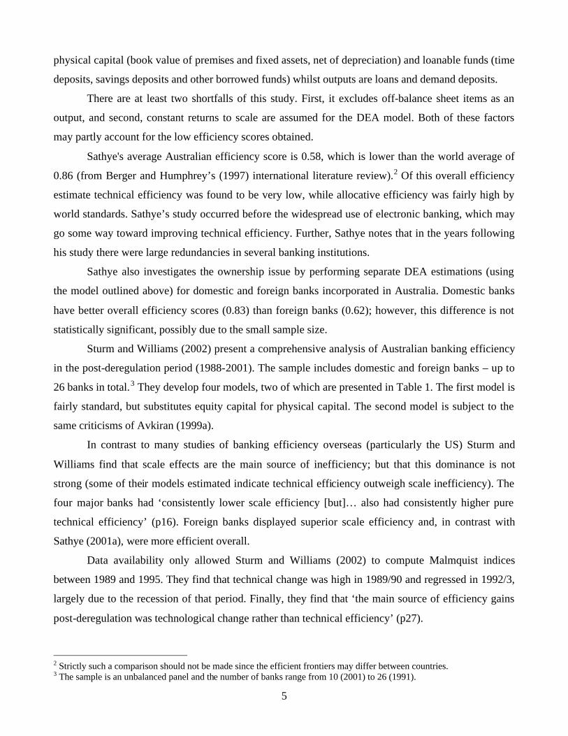
Table 1: A Summary of Australian Bank Cost Efficiency Studies4

Author(s) Method – scale assumption

Inputs Outputs Mean TE

(s.d.)

Mean AE(s.d.)

Mean SE (s.d.)

Mean CE (s.d.)

Interest expense, non-interest expense

Net interest income, non-interest income

N/A N/A N/A 0.79 (1991)-

0.91 (1986)

Avkiran (1999a)

DEA – CRTS

Deposits, staff numbers

Net loans, non-interest income

N/A N/A N/A 0.37 (1986) –

0.79 (1994)

Avkiran (1999b)5

DEA/Window analysis – VRTS

Interest expense, non-interest expense

Net interest income, non-interest income

0.956 (0.062)

N/A 0.985 (0.026)

0.942 (0.069)

Sathye (2001a)

DEA – CRTS Labour, capital, loanable funds

Loans, demand deposits

0.67 (0.17)

0.85 (0.11)

N/A 0.58 (0.18)

Staff numbers, deposits and borrowed funds, equity capital

Loans, and advance and receivables, off-balance sheet activity

0.86 (1991) –

0.99 (2000)

N/A 0.84 (1994)-

0.98 (2001)

0.73 (1991) –

0.94 (2000)

Sturm & Williams (2002)

DEA – VRTS

Interest expense, non-interest expense

Net interest income, non-interest income

0.89 (1988)-

0.98 (1997)

N/A 0.91 (1993)-

1.05 (1990)

0.67 (1993) –

0.91 (1996/8)

3. Model Development and Results

The majority of studies of Australian banking efficiency use DEA, largely because of the small

number of banks that may be included in the sample. Another advantage of using DEA is that no

functional form needs to be specified, which is ideal in the Australian case because although some

banks operate a fairly typical intermediation service, others offer a greater range of services. These

characteristics make the specification of a production function difficult and fraught with the probability

of using an incorrect functional form. The primary drawback of using DEA is that because it is a non-

parametric technique all deviations from the efficient frontier are assumed to arise from inefficiency –

that is, random error is not accounted for.

4 TE= technical efficiency, AE = allocative efficiency, and CE = cost efficiency. Recall CE = AE x TE. 5 Data for Avkiran (1999b) relates to 1995 only (the study was a panel data study)

8

3.1 Model Overview

Two models are estimated for this paper, and are summarised in Table 2.6 Both models adopt a

variation of the intermediation approach for measuring the efficiency of financial intermediaries, that

is, we view banks as intermediating between agents with surplus funds (depositors) and agents with

deficit funds (borrowers) (Sealey and Lindley, 1977).

Model A is a fairly standard model of cost efficiency using the intermediation approach, but

also accounts for off-balance sheet activity by incorporating non-interest income. An omission of off-

balance sheet activity from output (common in many studies of Australian banking efficiency) is likely

to result in understated measures of firm efficiency. Siems and Clark (2002) showed that non-interest

income provides a reasonable proxy for off-balance sheet activities. In summary, Model A views a

bank as using labour, physical capital and interest-bearing liabilities to produce interest-bearing assets

and non-interest income.

Labour is measured as the number of full-time equivalent employees the bank employs at the

end of the financial year. Physical capital is measured as the book value (cost less accumulated

depreciation) of property, plant and equipment. Both of these are standard measures of labour and

physical capital inputs used in the literature.

Average interest-bearing liabilities is a daily average reported by the banks and has been used

as an input because it includes deposits, the major source of on-balance sheet bank funding, and also

includes other sources of debt funding which the bank may substitute for deposit funding.

Prices for the inputs were calculated as follows: the price of labour, W1, equals staff expenses

divided by the number of full-time equivalent employees; the price of physical capital, W2, equals

expenses associated with property, plant and equipment divided by the book value of these assets at

year end, and finally; the price of interest-bearing liabilities, W3, equals interest expense divided by

average interest-bearing liabilities.

Average interest-bearing assets have been used as an output because it includes a more

comprehensive range of bank outputs than simply loans. The use of an average also has benefits.

Consider a bank that makes an abnormally large loan very close to the end of the financial year. If the

year-end stock of loans were used as the output, efficiency estimates for this bank may be biased

upwards, despite the increase in output coming only very close to the year-end. Similar reasoning can

be applied to average interest-bearing liabilities. Moreover, because non-interest income is a proxy for

6 DEAP software developed by T. Coelli has been used for all DEA estimations. This software is available from www.uq.edu.au/economics/cepa/

9

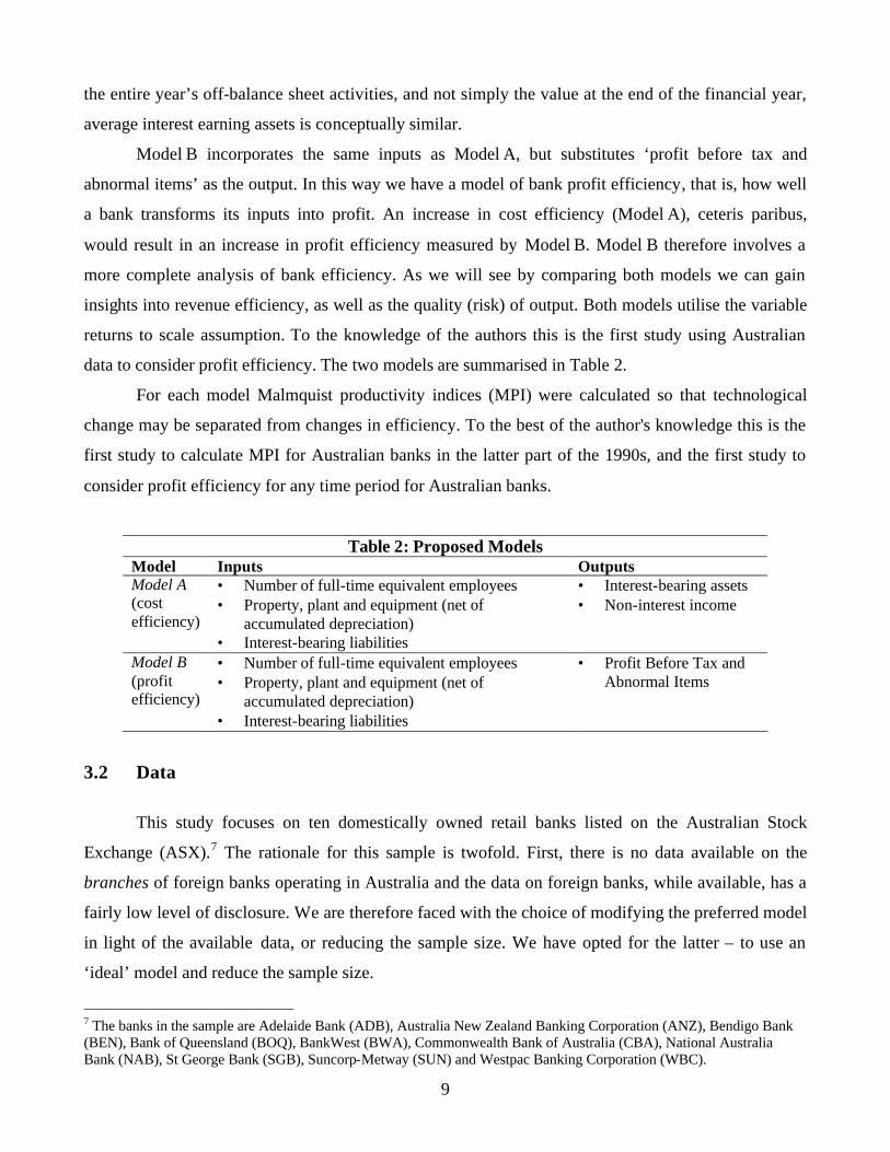
the entire year’s off-balance sheet activities, and not simply the value at the end of the financial year,

average interest earning assets is conceptually similar.

Model B incorporates the same inputs as Model A, but substitutes ‘profit before tax and

abnormal items’ as the output. In this way we have a model of bank profit efficiency, that is, how well

a bank transforms its inputs into profit. An increase in cost efficiency (Model A), ceteris paribus,

would result in an increase in profit efficiency measured by Model B. Model B therefore involves a

more complete analysis of bank efficiency. As we will see by comparing both models we can gain

insights into revenue efficiency, as well as the quality (risk) of output. Both models utilise the variable

returns to scale assumption. To the knowledge of the authors this is the first study using Australian

data to consider profit efficiency. The two models are summarised in Table 2.

For each model Malmquist productivity indices (MPI) were calculated so that technological

change may be separated from changes in efficiency. To the best of the author's knowledge this is the

first study to calculate MPI for Australian banks in the latter part of the 1990s, and the first study to

consider profit efficiency for any time period for Australian banks.

Table 2: Proposed Models Model Inputs Outputs Model A (cost efficiency)

• Number of full-time equivalent employees • Property, plant and equipment (net of

accumulated depreciation) • Interest-bearing liabilities

• Interest-bearing assets • Non-interest income

Model B (profit efficiency)

• Number of full-time equivalent employees • Property, plant and equipment (net of

accumulated depreciation) • Interest-bearing liabilities

• Profit Before Tax and Abnormal Items

3.2 Data

This study focuses on ten domestically owned retail banks listed on the Australian Stock

Exchange (ASX).7 The rationale for this sample is twofold. First, there is no data available on the

branches of foreign banks operating in Australia and the data on foreign banks, while available, has a

fairly low level of disclosure. We are therefore faced with the choice of modifying the preferred model

in light of the available data, or reducing the sample size. We have opted for the latter – to use an

‘ideal’ model and reduce the sample size.

7 The banks in the sample are Adelaide Bank (ADB), Australia New Zealand Banking Corporation (ANZ), Bendigo Bank (BEN), Bank of Queensland (BOQ), BankWest (BWA), Commonwealth Bank of Australia (CBA), National Australia Bank (NAB), St George Bank (SGB), Suncorp-Metway (SUN) and Westpac Banking Corporation (WBC).

10

The second reason for choosing the ten domestic banks listed on the ASX is that some analysis

can be performed of whether changes in efficiency are reflected in stock prices. This has only been

done once before in the literature, and we outline a method superior to that previously adopted (see

Section 4).

Data were obtained from annual reports for the selected period (1995 to 2002 inclusive).8

Accordingly there are 79 data observations – one for each bank for eight years (less Suncorp in 1997).

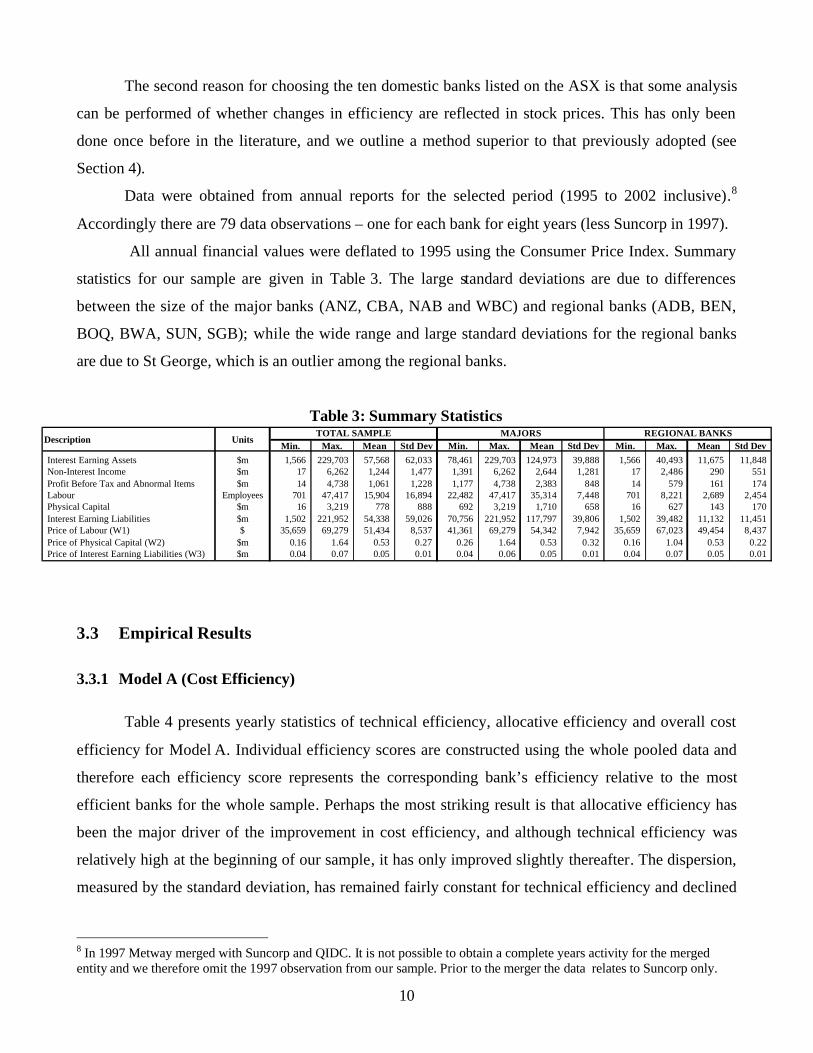
All annual financial values were deflated to 1995 using the Consumer Price Index. Summary

statistics for our sample are given in Table 3. The large standard deviations are due to differences

between the size of the major banks (ANZ, CBA, NAB and WBC) and regional banks (ADB, BEN,

BOQ, BWA, SUN, SGB); while the wide range and large standard deviations for the regional banks

are due to St George, which is an outlier among the regional banks.

Table 3: Summary Statistics

Min. Max. Mean Std Dev Min. Max. Mean Std Dev Min. Max. Mean Std DevInterest Earning Assets $m 1,566 229,703 57,568 62,033 78,461 229,703 124,973 39,888 1,566 40,493 11,675 11,848 Non-Interest Income $m 17 6,262 1,244 1,477 1,391 6,262 2,644 1,281 17 2,486 290 551 Profit Before Tax and Abnormal Items $m 14 4,738 1,061 1,228 1,177 4,738 2,383 848 14 579 161 174 Labour Employees 701 47,417 15,904 16,894 22,482 47,417 35,314 7,448 701 8,221 2,689 2,454 Physical Capital $m 16 3,219 778 888 692 3,219 1,710 658 16 627 143 170 Interest Earning Liabilities $m 1,502 221,952 54,338 59,026 70,756 221,952 117,797 39,806 1,502 39,482 11,132 11,451 Price of Labour (W1) $ 35,659 69,279 51,434 8,537 41,361 69,279 54,342 7,942 35,659 67,023 49,454 8,437 Price of Physical Capital (W2) $m 0.16 1.64 0.53 0.27 0.26 1.64 0.53 0.32 0.16 1.04 0.53 0.22 Price of Interest Earning Liabilities (W3) $m 0.04 0.07 0.05 0.01 0.04 0.06 0.05 0.01 0.04 0.07 0.05 0.01

DescriptionTOTAL SAMPLE MAJORS REGIONAL BANKS

Units

3.3 Empirical Results

3.3.1 Model A (Cost Efficiency)

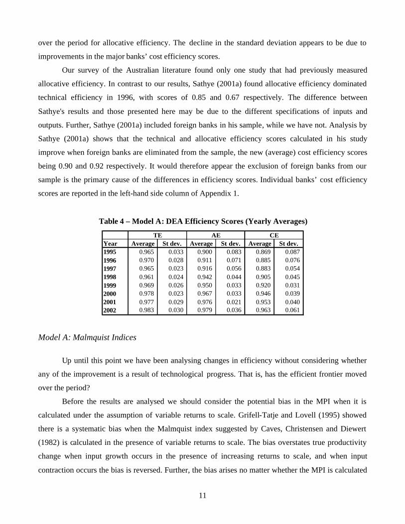
Table 4 presents yearly statistics of technical efficiency, allocative efficiency and overall cost

efficiency for Model A. Individual efficiency scores are constructed using the whole pooled data and

therefore each efficiency score represents the corresponding bank’s efficiency relative to the most

efficient banks for the whole sample. Perhaps the most striking result is that allocative efficiency has

been the major driver of the improvement in cost efficiency, and although technical efficiency was

relatively high at the beginning of our sample, it has only improved slightly thereafter. The dispersion,

measured by the standard deviation, has remained fairly constant for technical efficiency and declined

8 In 1997 Metway merged with Suncorp and QIDC. It is not possible to obtain a complete years activity for the merged entity and we therefore omit the 1997 observation from our sample. Prior to the merger the data relates to Suncorp only.

11

over the period for allocative efficiency. The decline in the standard deviation appears to be due to

improvements in the major banks’ cost efficiency scores.

Our survey of the Australian literature found only one study that had previously measured

allocative efficiency. In contrast to our results, Sathye (2001a) found allocative efficiency dominated

technical efficiency in 1996, with scores of 0.85 and 0.67 respectively. The difference between

Sathye's results and those presented here may be due to the different specifications of inputs and

outputs. Further, Sathye (2001a) included foreign banks in his sample, while we have not. Analysis by

Sathye (2001a) shows that the technical and allocative efficiency scores calculated in his study

improve when foreign banks are eliminated from the sample, the new (average) cost efficiency scores

being 0.90 and 0.92 respectively. It would therefore appear the exclusion of foreign banks from our

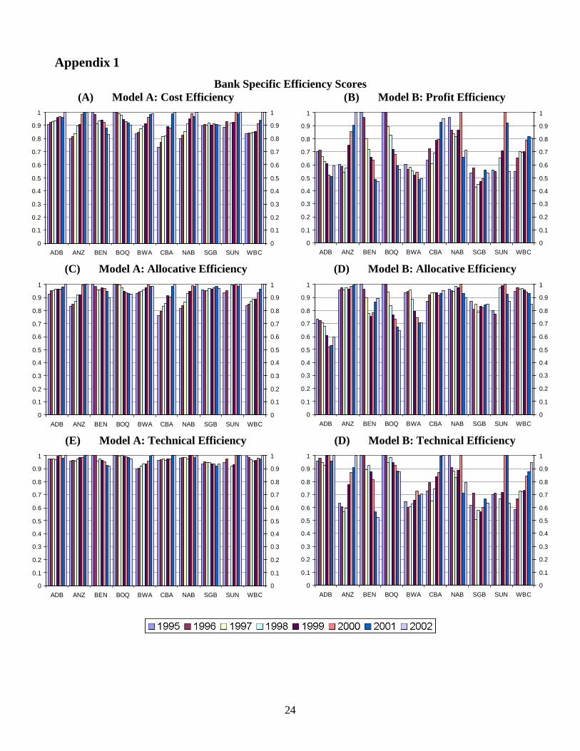
sample is the primary cause of the differences in efficiency scores. Individual banks’ cost efficiency

scores are reported in the left-hand side column of Appendix 1.

Table 4 – Model A: DEA Efficiency Scores (Yearly Averages)

Year Average St dev. Average St dev. Average St dev.1995 0.965 0.033 0.900 0.083 0.869 0.087 1996 0.970 0.028 0.911 0.071 0.885 0.076 1997 0.965 0.023 0.916 0.056 0.883 0.054 1998 0.961 0.024 0.942 0.044 0.905 0.045 1999 0.969 0.026 0.950 0.033 0.920 0.031 2000 0.978 0.023 0.967 0.033 0.946 0.039 2001 0.977 0.029 0.976 0.021 0.953 0.040 2002 0.983 0.030 0.979 0.036 0.963 0.061

TE AE CE

Model A: Malmquist Indices

Up until this point we have been analysing changes in efficiency without considering whether

any of the improvement is a result of technological progress. That is, has the efficient frontier moved

over the period?

Before the results are analysed we should consider the potential bias in the MPI when it is

calculated under the assumption of variable returns to scale. Grifell-Tatje and Lovell (1995) showed

there is a systematic bias when the Malmquist index suggested by Caves, Christensen and Diewert

(1982) is calculated in the presence of variable returns to scale. The bias overstates true productivity

change when input growth occurs in the presence of increasing returns to scale, and when input

contraction occurs the bias is reversed. Further, the bias arises no matter whether the MPI is calculated

12

using parametric or nonparametric approaches. Despite this theoretical flaw many studies of bank

efficiency calculate MPI under the assumption of variable returns to scale, with no mention of this

potential bias. The results presented here assume variable returns to scale; however, as we will see,

scale effects in our sample do not appear to be significant, and therefore the bias is unlikely to be

strong.

There is at least one other criticism of the approach adopted here. Since each Malmquist

‘window’ only incorporates 10 observations (10 banks) a high level of efficiency may not be

unexpected because with the variable returns to scale assumption many of these 10 observations may

be on the efficient frontier. To overcome this potential problem the MPI was also calculated using a

‘window’ of two periods (20 observations). The results were much the same as that presented here,

although the cumulative technological change was slightly less because of the ‘compounding’ effect

(the number of periods of compounding falls from 8 to 4). Under this approach (window length of 2

periods) cumulated technological change was 1.27 and the cumulative change in efficiency 0.98, which

is very similar to the results presented below.

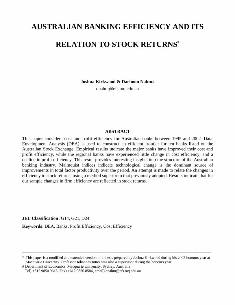
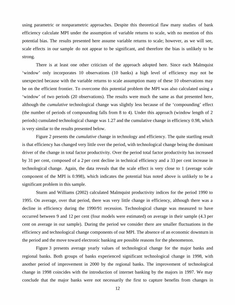
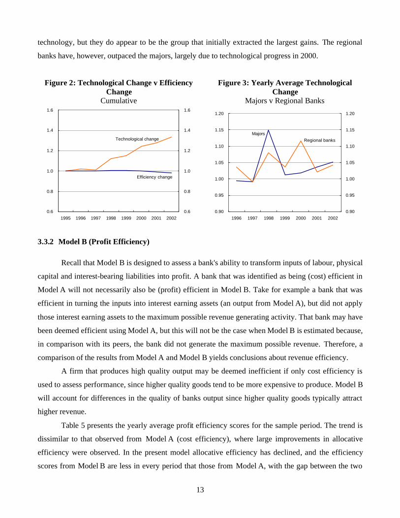
Figure 2 presents the cumulative change in technology and efficiency. The quite startling result

is that efficiency has changed very little over the period, with technological change being the dominant

driver of the change in total factor productivity. Over the period total factor productivity has increased

by 31 per cent, composed of a 2 per cent decline in technical efficiency and a 33 per cent increase in

technological change. Again, the data reveals that the scale effect is very close to 1 (average scale

component of the MPI is 0.998), which indicates the potential bias noted above is unlikely to be a

significant problem in this sample.

Sturm and Williams (2002) calculated Malmquist productivity indices for the period 1990 to

1995. On average, over that period, there was very little change in efficiency, although there was a

decline in efficiency during the 1990/91 recession. Technological change was measured to have

occurred between 9 and 12 per cent (four models were estimated) on average in their sample (4.3 per

cent on average in our sample). During the period we consider there are smaller fluctuations in the

efficiency and technological change components of our MPI. The absence of an economic downturn in

the period and the move toward electronic banking are possible reasons for the phenomenon.

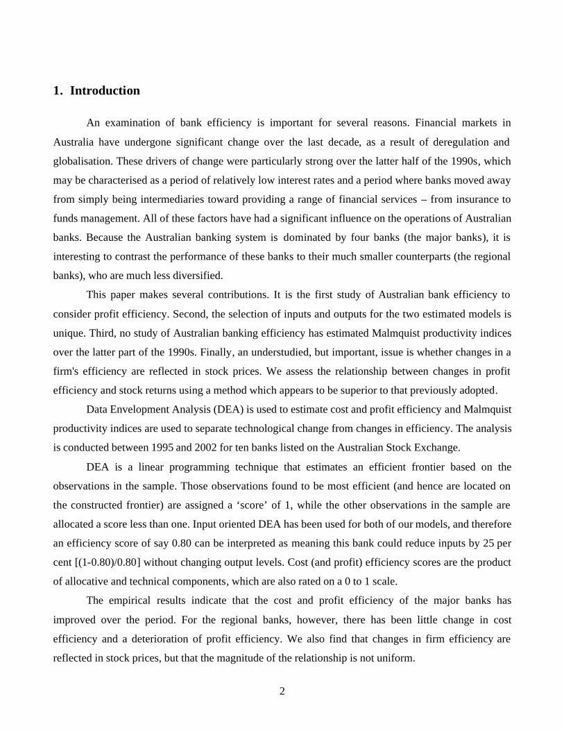
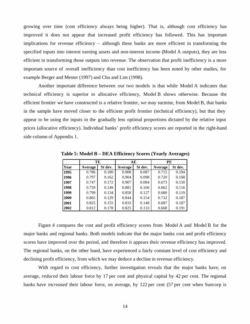
Figure 3 presents average yearly values of technological change for the major banks and

regional banks. Both groups of banks experienced significant technological change in 1998, with

another period of improvement in 2000 by the regional banks. The improvement of technological

change in 1998 coincides with the introduction of internet banking by the majors in 1997. We may

conclude that the major banks were not necessarily the first to capture benefits from changes in

13

technology, but they do appear to be the group that initially extracted the largest gains. The regional

banks have, however, outpaced the majors, largely due to technological progress in 2000.

Figure 2: Technological Change v Efficiency Change

Cumulative

Figure 3: Yearly Average Technological Change

Majors v Regional Banks

0.6

0.8

1.0

1.2

1.4

1.6

1995 1996 1997 1998 1999 2000 2001 20020.6

0.8

1.0

1.2

1.4

1.6

Technological change

Efficiency change

0.90

0.95

1.00

1.05

1.10

1.15

1.20

1996 1997 1998 1999 2000 2001 20020.90

0.95

1.00

1.05

1.10

1.15

1.20

MajorsRegional banks

3.3.2 Model B (Profit Efficiency)

Recall that Model B is designed to assess a bank's ability to transform inputs of labour, physical

capital and interest-bearing liabilities into profit. A bank that was identified as being (cost) efficient in

Model A will not necessarily also be (profit) efficient in Model B. Take for example a bank that was

efficient in turning the inputs into interest earning assets (an output from Model A), but did not apply

those interest earning assets to the maximum possible revenue generating activity. That bank may have

been deemed efficient using Model A, but this will not be the case when Model B is estimated because,

in comparison with its peers, the bank did not generate the maximum possible revenue. Therefore, a

comparison of the results from Model A and Model B yields conclusions about revenue efficiency.

A firm that produces high quality output may be deemed inefficient if only cost efficiency is

used to assess performance, since higher quality goods tend to be more expensive to produce. Model B

will account for differences in the quality of banks output since higher quality goods typically attract

higher revenue.

Table 5 presents the yearly average profit efficiency scores for the sample period. The trend is

dissimilar to that observed from Model A (cost efficiency), where large improvements in allocative

efficiency were observed. In the present model allocative efficiency has declined, and the efficiency

scores from Model B are less in every period that those from Model A, with the gap between the two

14

growing over time (cost efficiency always being higher). That is, although cost efficiency has

improved it does not appear that increased profit efficiency has followed. This has important

implications for revenue efficiency – although these banks are more efficient in transforming the

specified inputs into interest earning assets and non-interest income (Model A outputs), they are less

efficient in transforming those outputs into revenue. The observation that profit inefficiency is a more

important source of overall inefficiency than cost inefficiency has been noted by other studies, for

example Berger and Mester (1997) and Chu and Lim (1998).

Another important difference between our two models is that while Model A indicates that

technical efficiency is superior to allocative efficiency, Model B shows otherwise. Because the

efficient frontier we have constructed is a relative frontier, we may surmise, from Model B, that banks

in the sample have moved closer to the efficient profit frontier (technical efficiency), but that they

appear to be using the inputs in the gradually less optimal proportions dictated by the relative input

prices (allocative efficiency). Individual banks’ profit efficiency scores are reported in the right-hand

side column of Appendix 1.

Table 5: Model B – DEA Efficiency Scores (Yearly Averages)

Year Average St dev. Average St dev. Average St dev.1995 0.786 0.180 0.908 0.087 0.715 0.194 1996 0.797 0.162 0.904 0.098 0.720 0.168 1997 0.747 0.172 0.907 0.084 0.673 0.150 1998 0.759 0.149 0.881 0.106 0.662 0.116 1999 0.799 0.134 0.858 0.127 0.680 0.119 2000 0.865 0.129 0.844 0.154 0.732 0.187 2001 0.825 0.155 0.833 0.148 0.687 0.187 2002 0.812 0.178 0.825 0.133 0.668 0.191

TE AE PE

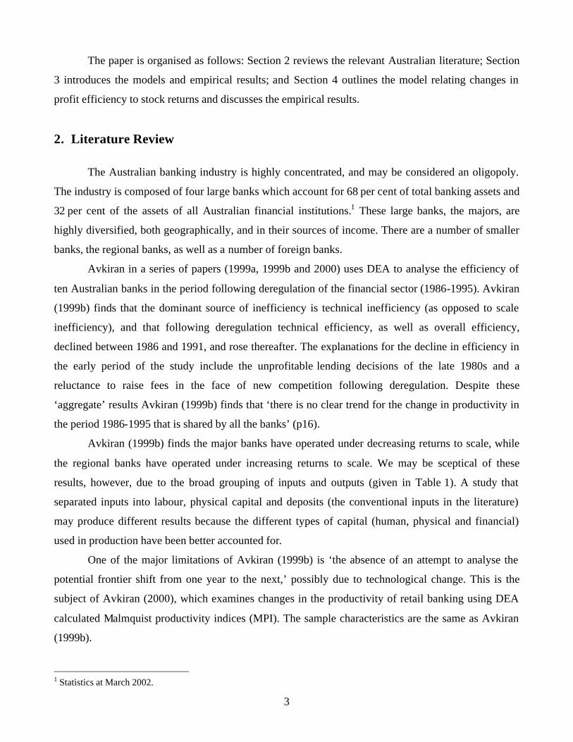
Figure 4 compares the cost and profit efficiency scores from Model A and Model B for the

major banks and regional banks. Both models indicate that the major banks cost and profit efficiency

scores have improved over the period, and therefore it appears their revenue efficiency has improved.

The regional banks, on the other hand, have experienced a fairly constant level of cost efficiency and

declining profit efficiency, from which we may deduce a decline in revenue efficiency.

With regard to cost efficiency, further investigation reveals that the major banks have, on

average, reduced their labour force by 17 per cent and physical capital by 42 per cent. The regional

banks have increased their labour force, on average, by 122 per cent (57 per cent when Suncorp is

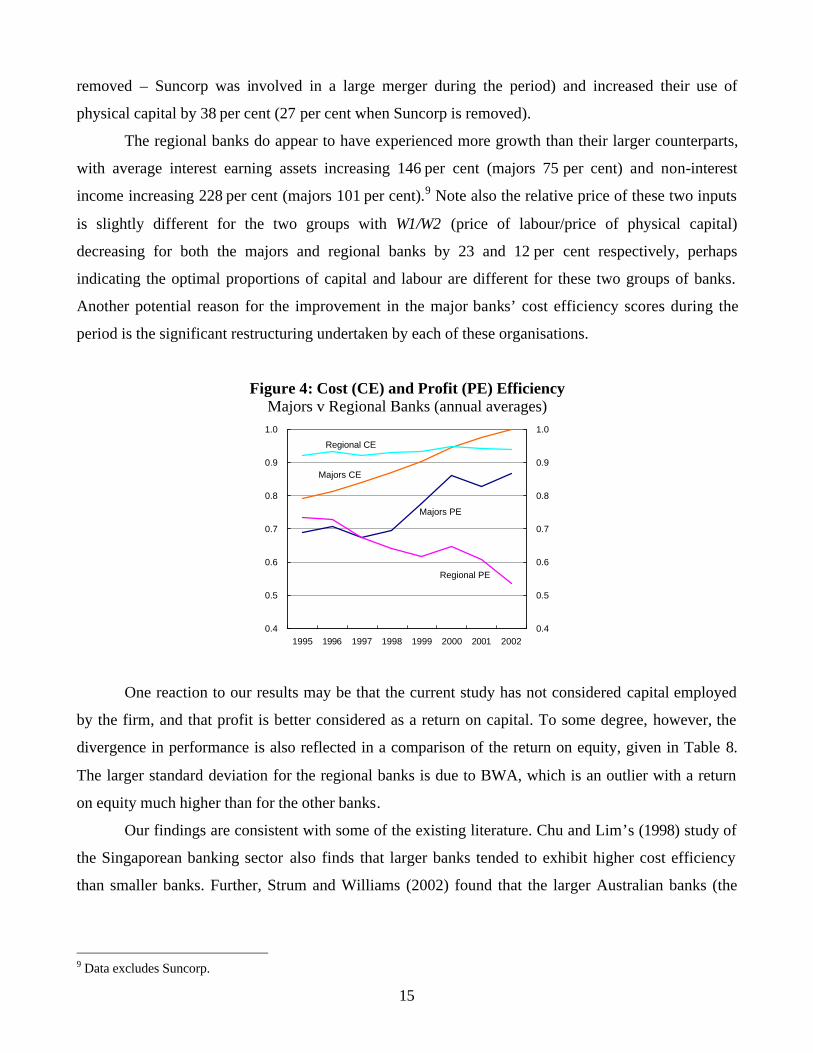
15

removed – Suncorp was involved in a large merger during the period) and increased their use of

physical capital by 38 per cent (27 per cent when Suncorp is removed).

The regional banks do appear to have experienced more growth than their larger counterparts,

with average interest earning assets increasing 146 per cent (majors 75 per cent) and non-interest

income increasing 228 per cent (majors 101 per cent).9 Note also the relative price of these two inputs

is slightly different for the two groups with W1/W2 (price of labour/price of physical capital)

decreasing for both the majors and regional banks by 23 and 12 per cent respectively, perhaps

indicating the optimal proportions of capital and labour are different for these two groups of banks.

Another potential reason for the improvement in the major banks’ cost efficiency scores during the

period is the significant restructuring undertaken by each of these organisations.

Figure 4: Cost (CE) and Profit (PE) Efficiency Majors v Regional Banks (annual averages)

0.4

0.5

0.6

0.7

0.8

0.9

1.0

1995 1996 1997 1998 1999 2000 2001 20020.4

0.5

0.6

0.7

0.8

0.9

1.0

Regional CE

Majors CE

Majors PE

Regional PE

One reaction to our results may be that the current study has not considered capital employed

by the firm, and that profit is better considered as a return on capital. To some degree, however, the

divergence in performance is also reflected in a comparison of the return on equity, given in Table 8.

The larger standard deviation for the regional banks is due to BWA, which is an outlier with a return

on equity much higher than for the other banks.

Our findings are consistent with some of the existing literature. Chu and Lim’s (1998) study of

the Singaporean banking sector also finds that larger banks tended to exhibit higher cost efficiency

than smaller banks. Further, Strum and Williams (2002) found that the larger Australian banks (the

9 Data excludes Suncorp.

16

major banks) tended to operate under decreasing returns to scale and exhibited higher technical

efficiency.

Table 6: Return on Equity 1995 1996 1997 1998 1999 2000 2001 2002 Average

MajorsAverage 15.50 16.00 16.88 16.48 16.70 16.03 16.18 17.23 16.37 St dev. 1.98 1.64 1.11 1.56 0.85 4.46 3.88 3.34 2.41

Regional BanksAverage 14.37 13.03 10.82 11.65 11.38 12.35 12.82 13.17 12.45 St dev. 3.20 3.16 4.30 3.39 4.10 3.21 2.47 2.61 3.28

Source: Datastream

The better performance of the major banks yields several conclusions. First, it has been noted

that the major banks are far more than a typical bank intermediaries – each of them derive significant

revenue from funds management, insurance, and other activities. The major banks are also far more

geographically diversified than the regional banks. Therefore, compared to their regional counterparts,

the major banks have a more diversified income stream, and are less reliant on Australian interest

income.

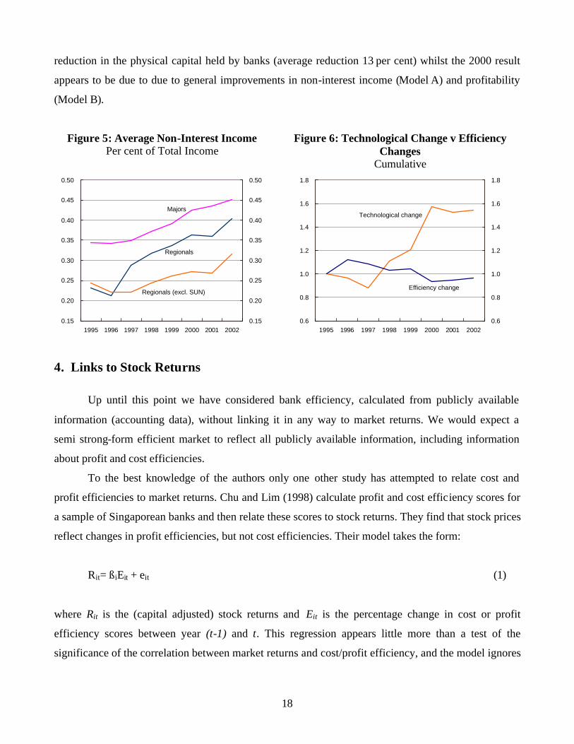
Figure 5 presents the average proportion of non-interest income to total income for the majors

and regional banks. Clearly the regional banks have a less diversified income stream. Suncorp (SUN)

is an outlier of the regional banks because it derives a large proportion of income from insurance

activities (in 2002 over 80 per cent of income was non-interest income, of which the majority was

income from insurance activities). The jump in the regional bank proportion of non-interest income in

1997 is due to Suncorp’s merger with Metway in that year. When Suncorp is removed the difference

between the major banks and regional banks becomes even more stark.

In a period of declining interest rates the contribution of each unit of net interest earning assets

(interest earning assets less interest earning liabilities) to revenue declines, provided the interest spread

also declines. The data in the current sample indicates the interest spread has declined for every bank,

likely reflecting a number of factors including the globalisation of financial markets, increased

competition (for example by mortgage managers) and a low interest rate environment.

Ceteris paribus, a decline in the interest spread would result in a reduction in profit and hence a

reduction in profit efficiency as it has been calculated here. This conclusion is consistent with the

decline in regional bank profit efficiency, since the regional banks rely more on domestic interest

income. The relative improvement in revenue efficiency for the major banks therefore indicates these

banks have avoided reductions in profit efficiency through revenue diversification. Further, because of

17

the improvement in cost efficiency experienced by the major banks and their growth of non-interest

income, it appears there may be economies of scope in the provision of typical bank intermediation

and some other financial services (funds management and insurance for example).

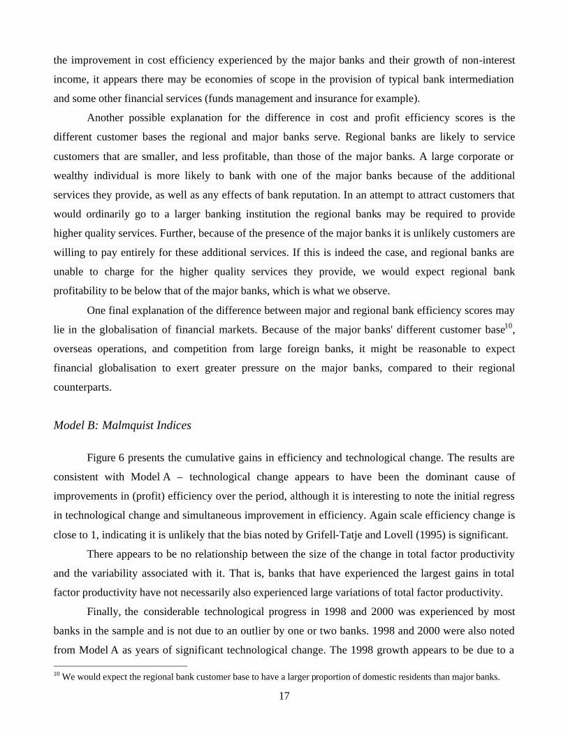
Another possible explanation for the difference in cost and profit efficiency scores is the

different customer bases the regional and major banks serve. Regional banks are likely to service

customers that are smaller, and less profitable, than those of the major banks. A large corporate or

wealthy individual is more likely to bank with one of the major banks because of the additional

services they provide, as well as any effects of bank reputation. In an attempt to attract customers that

would ordinarily go to a larger banking institution the regional banks may be required to provide

higher quality services. Further, because of the presence of the major banks it is unlikely customers are

willing to pay entirely for these additional services. If this is indeed the case, and regional banks are

unable to charge for the higher quality services they provide, we would expect regional bank

profitability to be below that of the major banks, which is what we observe.

One final explanation of the difference between major and regional bank efficiency scores may

lie in the globalisation of financial markets. Because of the major banks' different customer base10,

overseas operations, and competition from large foreign banks, it might be reasonable to expect

financial globalisation to exert greater pressure on the major banks, compared to their regional

counterparts.

Model B: Malmquist Indices

Figure 6 presents the cumulative gains in efficiency and technological change. The results are

consistent with Model A – technological change appears to have been the dominant cause of

improvements in (profit) efficiency over the period, although it is interesting to note the initial regress

in technological change and simultaneous improvement in efficiency. Again scale efficiency change is

close to 1, indicating it is unlikely that the bias noted by Grifell-Tatje and Lovell (1995) is significant.

There appears to be no relationship between the size of the change in total factor productivity

and the variability associated with it. That is, banks that have experienced the largest gains in total

factor productivity have not necessarily also experienced large variations of total factor productivity.

Finally, the considerable technological progress in 1998 and 2000 was experienced by most

banks in the sample and is not due to an outlier by one or two banks. 1998 and 2000 were also noted

from Model A as years of significant technological change. The 1998 growth appears to be due to a 10 We would expect the regional bank customer base to have a larger proportion of domestic residents than major banks.

18

reduction in the physical capital held by banks (average reduction 13 per cent) whilst the 2000 result

appears to be due to due to general improvements in non-interest income (Model A) and profitability

(Model B).

Figure 5: Average Non-Interest Income Per cent of Total Income

Figure 6: Technological Change v Efficiency Changes

Cumulative

0.15

0.20

0.25

0.30

0.35

0.40

0.45

0.50

1995 1996 1997 1998 1999 2000 2001 20020.15

0.20

0.25

0.30

0.35

0.40

0.45

0.50

Majors

Regionals

Regionals (excl. SUN)

0.6

0.8

1.0

1.2

1.4

1.6

1.8

1995 1996 1997 1998 1999 2000 2001 20020.6

0.8

1.0

1.2

1.4

1.6

1.8

Technological change

Efficiency change

4. Links to Stock Returns

Up until this point we have considered bank efficiency, calculated from publicly available

information (accounting data), without linking it in any way to market returns. We would expect a

semi strong-form efficient market to reflect all publicly available information, including information

about profit and cost efficiencies.

To the best knowledge of the authors only one other study has attempted to relate cost and

profit efficiencies to market returns. Chu and Lim (1998) calculate profit and cost efficiency scores for

a sample of Singaporean banks and then relate these scores to stock returns. They find that stock prices

reflect changes in profit efficiencies, but not cost efficiencies. Their model takes the form:

Rit= ßiEit + eit (1)

where Rit is the (capital adjusted) stock returns and Eit is the percentage change in cost or profit

efficiency scores between year (t-1) and t. This regression appears little more than a test of the

significance of the correlation between market returns and cost/profit efficiency, and the model ignores

19

other factors which may affect stock returns. That is, the model is likely to omit relevant variables and

therefore estimates will be biased.

To consider this problem we specify a model of excess stock returns which includes profit

efficiency as an explanatory variable. We build upon the Sharpe-Lintner’s excess-returns version of the

Capital Asset Pricing Model (CAPM). The model takes the form:

ERit = a i + ßi EMt+ di PEit + eit (2)

where ERit is the excess return on stock i in time t (excess return is the return on stock i, less the risk

free rate), EMt is the excess market return, and PEit is the percentage change in profit efficiency. eit is a

random error term. If the original version of the model is valid for the current data, the intercept term,

αi, and the coefficient of PEit, δi, will have to be zero. If either of the two coefficients turned out to be

different from zero, it might imply that the market portfolio is not mean-variance efficient.11

Recall that profit efficiency (Model B) incorporated both revenue efficiency and cost efficiency

considerations. From a comparison of profit efficiency and cost efficiency (Model A) we were able to

draw inferences about revenue efficiency. Since profit efficiency captures both cost and revenue

efficiency it is sufficient to include only profit efficiency in the model to capture the effect of changes

in the firm’s efficiency.

4.1 The Data

Because annual data have been used to calculate profit and cost efficiency scores, stock returns are

calculated based on the same time period. ERit, the excess stock return, consists of two components:

the stock return and the risk-free return. The stock return consists of the dividend return and the return

from movements in the stock price. Stock returns have been calculated as the sum of monthly returns.

The average annualised monthly return on 90 day Treasury Notes for the relevant banks’ financial year

is used as a proxy for the risk free return.

Again, EMt is the excess return on the market and is composed of the market return less a risk-

free component. The FTSE Australia price index (from DataStream) has been used as the market

portfolio and the return on this portfolio is calculated in the same manner as for individual stock

11 To make a more conclusive statement regarding this point would require a joint significance test including other stocks as well as banking stocks.

20

returns.12 Finally PEit is the percentage change in cost and profit efficiency scores calculated from

Section 3.

Because the percentage change in profit efficiency scores were used 10 observations (one for

each bank) were lost from the initial sample. A further three observations were removed from the

sample: BWA was not listed until February 1996, and therefore the 1995 and 1996 observations could

not be included in the regression. The Suncorp 1997 observation has also been removed since complete

data could not be obtained to calculate profit efficiency scores. We therefore have 67 observations in

total.

4.2 Empirical Results

To operationalise equation (6) we utilise dummy variables to re-specify the model as:

it

10

1iititi

10

1iititiit

9

1iiit PEDEMDDER ε+δ+β+α= ∑∑∑

===

for t = 1996, ..., 2002 and i = 1, ..,10 (3)

where Dit= 1 for bank i, and 0 otherwise. The random errors are assumed to be serially uncorrelated.

As the notation indicates one intercept dummy (the dummy for WBC) and the EM and PE terms were

dropped to avoid the dummy variable trap. Subscript “i” has been added to EM to note that different

market returns are applied to the banks with different financial years. With only 9 time-series

observations for each bank, it would obviously be difficult to estimate the coefficients with high

precision if a separate model were estimated for each bank. An F-test on the null hypothesis that the

banks could be grouped into the major banks (ANZ, CBA, NAB and WBC) and the regional banks

(ADB, BEN, BOQ, BWA, SGB, and SUN) was carried out, and the null could not be rejected, even at

70 per cent, implying that the information from the sample is consistent with the grouping (F24,37 =

0.793, p-value = 0.722).

12 The more common All Ordinaries market index was also tested; however, problems arose in estimation with this index because, on average, over the period the risk free rate exceeded the return on the All Ordinaries (average excess market return was negative and equal to -0.177 per cent). The FTSE Australia index is an index compiled by FTSE for use in their FTSE All-World Index and other indices. Its correlation with the All Ordinaries during the sample period is 0.94 and consists of 111 companies listed on the ASX.

21

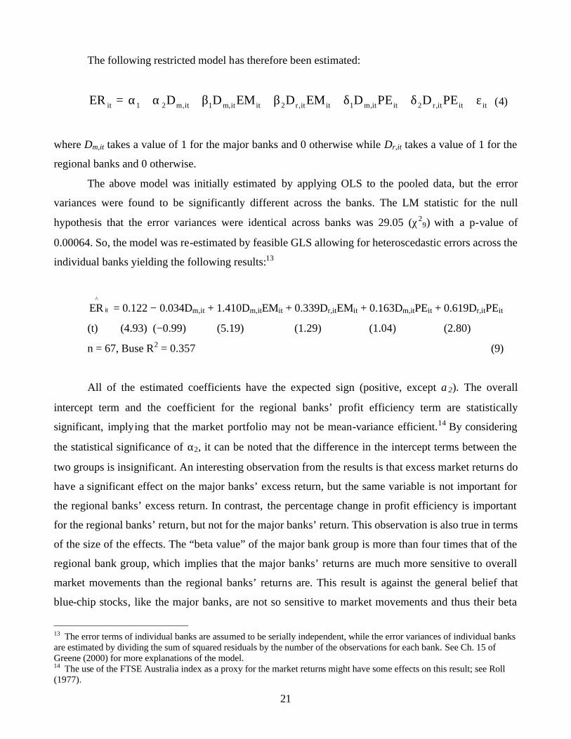
The following restricted model has therefore been estimated:

ititit,r2itit,m1itit,r2itit,m1it,m21it PEDPEDEMDEMDDER ε+δ+δ+β+β+α+α= (4)

where Dm,it takes a value of 1 for the major banks and 0 otherwise while Dr,it takes a value of 1 for the

regional banks and 0 otherwise.

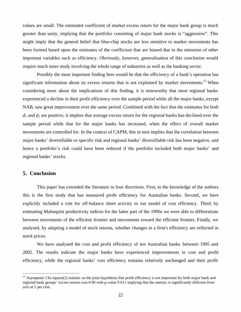
The above model was initially estimated by applying OLS to the pooled data, but the error

variances were found to be significantly different across the banks. The LM statistic for the null

hypothesis that the error variances were identical across banks was 29.05 (χ29) with a p-value of

0.00064. So, the model was re-estimated by feasible GLS allowing for heteroscedastic errors across the

individual banks yielding the following results:13

it

^

ER = 0.122 − 0.034Dm,it + 1.410Dm,itEMit + 0.339Dr,itEMit + 0.163Dm,itPEit + 0.619Dr,itPEit

(t) (4.93) (−0.99) (5.19) (1.29) (1.04) (2.80)

n = 67, Buse R2 = 0.357 (9)

All of the estimated coefficients have the expected sign (positive, except α2). The overall

intercept term and the coefficient for the regional banks’ profit efficiency term are statistically

significant, implying that the market portfolio may not be mean-variance efficient.14 By considering

the statistical significance of α2, it can be noted that the difference in the intercept terms between the

two groups is insignificant. An interesting observation from the results is that excess market returns do

have a significant effect on the major banks’ excess return, but the same variable is not important for

the regional banks’ excess return. In contrast, the percentage change in profit efficiency is important

for the regional banks’ return, but not for the major banks’ return. This observation is also true in terms

of the size of the effects. The “beta value” of the major bank group is more than four times that of the

regional bank group, which implies that the major banks’ returns are much more sensitive to overall

market movements than the regional banks’ returns are. This result is against the general belief that

blue-chip stocks, like the major banks, are not so sensitive to market movements and thus their beta

13 The error terms of individual banks are assumed to be serially independent, while the error variances of individual banks are estimated by dividing the sum of squared residuals by the number of the observations for each bank. See Ch. 15 of Greene (2000) for more explanations of the model. 14 The use of the FTSE Australia index as a proxy for the market returns might have some effects on this result; see Roll (1977).

22

values are small. The estimated coefficient of market excess return for the major bank group is much

greater than unity, implying that the portfolio consisting of major bank stocks is “aggressive”. This

might imply that the general belief that blue-chip stocks are less sensitive to market movements has

been formed based upon the estimates of the coefficient that are biased due to the omission of other

important variables such as efficiency. Obviously, however, generalisation of this conclusion would

require much more study involving the whole range of industries as well as the banking sector.

Possibly the most important finding here would be that the efficiency of a bank’s operation has

significant information about its excess returns that is not explained by market movements.15 When

considering more about the implications of this finding, it is noteworthy that most regional banks

experienced a decline in their profit efficiency over the sample period while all the major banks, except

NAB, saw great improvement over the same period. Combined with the fact that the estimates for both

δ1 and δ2 are positive, it implies that average excess return for the regional banks has declined over the

sample period while that for the major banks has increased, when the effect of overall market

movements are controlled for. In the context of CAPM, this in turn implies that the correlation between

major banks’ diversifiable or specific risk and regional banks’ diversifiable risk has been negative, and

hence a portfolio’s risk could have been reduced if the portfolio included both major banks’ and

regional banks’ stocks.

5. Conclusion

This paper has extended the literature in four directions. First, to the knowledge of the authors

this is the first study that has measured profit efficiency for Australian banks. Second, we have

explicitly included a role for off-balance sheet activity in our model of cost efficiency. Third, by

estimating Malmquist productivity indices for the latter part of the 1990s we were able to differentiate

between movements of the efficient frontier and movements toward the efficient frontier. Finally, we

analysed, by adapting a model of stock returns, whether changes in a firm's efficiency are reflected in

stock prices.

We have analysed the cost and profit efficiency of ten Australian banks between 1995 and

2002. The results indicate the major banks have experienced improvements in cost and profit

efficiency, while the regional banks’ cost efficiency remains relatively unchanged and their profit

15 Asymptotic Chi-square(2) statistic on the joint hypothesis that profit efficiency is not important for both major bank and regional bank groups’ excess returns was 8.90 with p-value 0.011 implying that the statistic is significantly different from zero at 5 per cent.

23

efficiency has declined. The regional banks had relatively high cost efficiency initially, and up until

2000 the majors and regional bank cost efficiency scores converged. By combining the results of

Model A (cost efficiency) and Model B (profit efficiency) we can infer that revenue efficiency has

declined for the regional banks, but improved for the major banks.

Possible explanations for the differing efficiency scores for the majors and regional banks were

given, including conglomeration, organisational restructuring, different customer bases of the two

groups of banks, and the effects of the globalisation of financial services.

MPI were calculated to separate movements in the efficient frontier (technological change)

from movements toward the efficient frontier (changes in efficiency). Our results indicate that

technological change has been the major contributor to improvements in total factor productivity over

the period, with 1998 and 2000 being identified as years of considerable technological progress.

It was also shown that changes in profit efficiency are statistically significant in determining

the stock returns of banks, particularly the regional banks, in our sample. Previous studies have

calculated efficiency scores without reference to market judgements of efficiency. One implication of

our results is that the Australian equities market (ASX) appears to be semi-strong form efficient. That

is, all publicly available information regarding the prospects of a firm is reflected in the stock price.

24

Appendix 1

Bank Specific Efficiency Scores (A) Model A: Cost Efficiency (B) Model B: Profit Efficiency

0

0.1

0.2

0.3

0.4

0.5

0.6

0.7

0.8

0.9

1

ADB ANZ BEN BOQ BWA CBA NAB SGB SUN WBC0

0.1

0.2

0.3

0.4

0.5

0.6

0.7

0.8

0.9

1

0

0.1

0.2

0.3

0.4

0.5

0.6

0.7

0.8

0.9

1

ADB ANZ BEN BOQ BWA CBA NAB SGB SUN WBC0

0.1

0.2

0.3

0.4

0.5

0.6

0.7

0.8

0.9

1

(C) Model A: Allocative Efficiency (D) Model B: Allocative Efficiency

0

0.1

0.2

0.3

0.4

0.5

0.6

0.7

0.8

0.9

1

ADB ANZ BEN BOQ BWA CBA NAB SGB SUN WBC0

0.1

0.2

0.3

0.4

0.5

0.6

0.7

0.8

0.9

1

0

0.1

0.2

0.3

0.4

0.5

0.6

0.7

0.8

0.9

1

ADB ANZ BEN BOQ BWA CBA NAB SGB SUN WBC0

0.1

0.2

0.3

0.4

0.5

0.6

0.7

0.8

0.9

1

(E) Model A: Technical Efficiency (D) Model B: Technical Efficiency

0

0.1

0.2

0.3

0.4

0.5

0.6

0.7

0.8

0.9

1

ADB ANZ BEN BOQ BWA CBA NAB SGB SUN WBC0

0.1

0.2

0.3

0.4

0.5

0.6

0.7

0.8

0.9

1

0

0.1

0.2

0.3

0.4

0.5

0.6

0.7

0.8

0.9

1

ADB ANZ BEN BOQ BWA CBA NAB SGB SUN WBC0

0.1

0.2

0.3

0.4

0.5

0.6

0.7

0.8

0.9

1

25

References

Avkiran, Necmi (1999a). “The Evidence on Efficiency Gains: The Role of Mergers and the Benefits to

the Public.” Journal of Banking and Finance 23 (7), 991-1013.

Avkiran, Necmi (1999b). “Decomposing the Technical Efficiency of Trading Banks in the Deregulated

Period.” 12th Australasian Finance and Banking Conference, The University of New South Wales,

Sydney.

Avkiran, Necmi (2000). “Rising Productivity of Australian Trading Banks Under Deregulation 1986-

1995.” Journal of Economics and Finance 24 (2), 122-140.

Berger, Alan, and David B. Humphrey. (1997). “Efficiency of Financial Institutions: International

Survey and Directions for Future Research.” European Journal of Operational Research 98, 175-212.

Caves, D. W., Laurits R. Christensen, and W. Erwin Diewert. (1982). “The Economic Theory of Index

Numbers and the Measurement of Input, Output, and Productivity.” Econometrica 50, 1393-1414.

Berger, Alan, and Loretta J. Mester (1997). “Inside the Black Box: What Explains Differences in

Efficiencies of Financial Institutions?” Journal of Banking and Finance 21, 895-947.

Chu, Sing Fat and Guan Hua Lim (1998). “Share Market Performance and Profit Efficiency of Banks

in an Oligopolistic Market: Evidence from Singapore.” Journal of Multinational Financial

Management 8, 155-168.

Coelli, Tim (1996). “A Guide to DEAP Version 2.1: A Data Analysis (Computer) Program.” Centre

for Efficiency and Productivity Analysis (CEPA) Working Papers 8/96, The University of New

England, 1996.

Greene, William H. (2000). Econometric Analysis, 4th edition. Upper Saddle River, NJ: Prentice Hall.

Grifell-Tatje, Emili, and C.A. Knox Lovell (1995). “A Note on the Malmquist Productivity Index.”

Economic Letters 47, 169-175.

26

Roll, Richard (1977). “A Critique of the Asset Pricing Theory’s Tests.” Journal of Financial

Economics 4, 129-176.

Sathye, Milind (2001a). “X-efficiency in Australian Banking: An Empirical Investigation." Journal of

Banking and Finance 25, 613-630.

Sathye, Milind (2001b). “Growth of Internet Banking in Australia.” Unpublished, University of

Southern Queensland.

Sealey, Calvin W., and James T. Lindley. (1977). “Inputs, Outputs, and a Theory of Production and

Cost at Depository Financial Institutions.” The Journal of Finance 37(4), 1251-1266.

Siems, Thomas F., and Jeffery A. Clark. (1997). “Rethinking Bank Efficiency and Regulation: How

Off-Balance-Sheet Activities Make A Difference.” Federal Reserve Bank of Dallas Financial Industry

Studies, December 1997, 1-12.

Siems, Thomas F., and Jeffery A. Clark. (2002). “X-Efficiency in Banking: Looking Beyond the

Balance Sheet.” Journal of Money, Credit, and Banking 34(4), 987-1013.

Sturm, Jan-Egbert and Barry W. Williams. (2002). “Deregulation, Entry of Foreign Banks and Bank

Efficiency in Australia.” CESifo Working Paper no. 816, Category 9: Industrial Organisation,

December 2002, downloaded from www.CESifo.de