AUSERGUIDE FORDRAGON VERSION4 G. Marleau, A. H´ebert and …

TECHNICAL REPORTIGE–294

A USER GUIDE FOR DRAGON VERSION4

G. Marleau, A. Hebert and R. Roy

Institut de genie nucleaireDepartement de genie mecanique

Ecole Polytechnique de MontrealAugust 26, 2016

IGE–294 ii

Copyright Notice for DRAGON

The development of DRAGON is financially supported, directly or indirectly, by various organiza-tions including Ecole Polytechnique de Montreal, Hydro–Quebec and the Hydro–Quebec chair in nuclearengineering, the Natural Science and Engineering Research Council of Canada (NSERC), Atomic Energyof Canada limited (AECL) and the CANDU Owners Group (COG). The code DRAGON and its usersguide are and will remain the property of Ecole Polytechnique de Montreal. The PostScript utility moduleused in DRAGON is based on PSPLOT which is owned by Kevin E. Kohler at the Nova SoutheasternUniversity Oceanographic Center in Florida.

Dragon is free software; you can redistribute it and/or modify it under the terms of the GNU LesserGeneral Public License as published by the Free Software Foundation; either version 2.1 of the License,or (at your option) any later version.

Permission is granted to the public to copy DRAGON without charge. Ecole Polytechnique deMontreal, makes no warranty, express or implied, and assumes no liability or responsibility for the use ofDRAGON.

IGE–294 iii

Acknowledgments

The computer code DRAGON results from a concerted effort made at Ecole Polytechnique de Montreal.The main authors of this report would therefore like to express their thanks to Ecole Polytechnique deMontreal for its support along the years as well as to the graduate students and research associates whichhave contributed to the development of DRAGON along the years. We would also like to thank KevinE. Kohler at the Nova Southeastern University Oceanographic Center for letting us use and distribute aPostScript utility module derived from his PSPLOT package. Finally, the DRAGON team would neverhave survived without the financial support of the Natural Science and Engineering Research Council ofCanada (NSERC), Hydro–Quebec, Atomic Energy of Canada limited (AECL) and the CANDU OwnersGroup (COG).

IGE–294 iv

SUMMARY

The computer code DRAGON contains a collection of models which can simulate the neutronic be-haviour of a unit cell or a fuel assembly in a nuclear reactor. It includes all of the functions thatcharacterize a lattice cell code, namely: the interpolation of microscopic cross sections which are sup-plied by means of standard libraries; resonance self-shielding calculations in multidimensional geometries;multigroup and multidimensional neutron flux calculations which can take into account neutron leakage;transport-transport or transport-diffusion equivalence calculations as well as editing of condensed andhomogenized nuclear properties for reactor calculations; and finally isotopic depletion calculations.

The code DRAGON contains a multigroup iterator conceived to control a number of different algo-rithms for the solution of the neutron transport equation. Each of these algorithms is presented in theform of a one-group solution procedure where the contributions from other energy groups are included in asource term. The current version of DRAGON contains many such algorithms. The SYBIL option whichsolves the integral transport equation using the collision probability method for simple one-dimensional(1–D) geometries (either plane, cylindrical or spherical) and the interface current method for 2–D Carte-sian or hexagonal assemblies. The EXCELL option which solves the integral transport equation using thecollision probability method for general 2–D geometries and for three-dimensional (3–D) assemblies. TheMCCG option solves the integro-differential transport equation using the long characteristics method forgeneral 2–D and 3–D geometries.

The execution of DRAGON is controlled by the generalized GAN driver. It is modular and can beinterfaced easily with other production codes.

IGE–294 v

Contents

Copyright Notice for DRAGON . . . . . . . . . . . . . . . . . . . . . . . . . . . . . . . . . . . iiAcknowledgments . . . . . . . . . . . . . . . . . . . . . . . . . . . . . . . . . . . . . . . . . . . iiiContents . . . . . . . . . . . . . . . . . . . . . . . . . . . . . . . . . . . . . . . . . . . . . . . . vList of Figures . . . . . . . . . . . . . . . . . . . . . . . . . . . . . . . . . . . . . . . . . . . . . viiiList of Tables . . . . . . . . . . . . . . . . . . . . . . . . . . . . . . . . . . . . . . . . . . . . . ix1 INTRODUCTION . . . . . . . . . . . . . . . . . . . . . . . . . . . . . . . . . . . . . . . . 12 GENERAL STRUCTURE OF THE DRAGON INPUT . . . . . . . . . . . . . . . . . . . 2

2.1 Data organization . . . . . . . . . . . . . . . . . . . . . . . . . . . . . . . . . . . . 22.2 DRAGON Data Structure and Module Declarations . . . . . . . . . . . . . . . . . 32.3 The DRAGON Modules . . . . . . . . . . . . . . . . . . . . . . . . . . . . . . . . . 42.4 The Utility Modules . . . . . . . . . . . . . . . . . . . . . . . . . . . . . . . . . . . 62.5 The DRAGON Data Structures . . . . . . . . . . . . . . . . . . . . . . . . . . . . . 62.6 Main Updates in DRAGON . . . . . . . . . . . . . . . . . . . . . . . . . . . . . . . 7

3 THE DRAGON MODULES . . . . . . . . . . . . . . . . . . . . . . . . . . . . . . . . . . 93.1 The MAC: module . . . . . . . . . . . . . . . . . . . . . . . . . . . . . . . . . . . . . 9

3.1.1 Input structure for module MAC: . . . . . . . . . . . . . . . . . . . . . . . 103.1.2 Macroscopic cross section definition . . . . . . . . . . . . . . . . . . . . . 123.1.3 Update structure for operator MAC: . . . . . . . . . . . . . . . . . . . . . 14

3.2 The LIB: module . . . . . . . . . . . . . . . . . . . . . . . . . . . . . . . . . . . . . 163.2.1 Data input for module LIB: . . . . . . . . . . . . . . . . . . . . . . . . . 163.2.2 Depletion data structure . . . . . . . . . . . . . . . . . . . . . . . . . . . 223.2.3 Mixture description structure . . . . . . . . . . . . . . . . . . . . . . . . . 23

3.3 The GEO: module . . . . . . . . . . . . . . . . . . . . . . . . . . . . . . . . . . . . . 293.3.1 Data input for module GEO: . . . . . . . . . . . . . . . . . . . . . . . . . 293.3.2 Boundary conditions . . . . . . . . . . . . . . . . . . . . . . . . . . . . . . 323.3.3 Spatial properties of geometry . . . . . . . . . . . . . . . . . . . . . . . . 413.3.4 Physical properties of geometry . . . . . . . . . . . . . . . . . . . . . . . 463.3.5 Double-heterogeneity . . . . . . . . . . . . . . . . . . . . . . . . . . . . . 563.3.6 Do-it-yourself geometries . . . . . . . . . . . . . . . . . . . . . . . . . . . 56

3.4 The tracking modules . . . . . . . . . . . . . . . . . . . . . . . . . . . . . . . . . . 583.4.1 The SYBILT: tracking module . . . . . . . . . . . . . . . . . . . . . . . . 603.4.2 The EXCELT: tracking module . . . . . . . . . . . . . . . . . . . . . . . . 633.4.3 The NXT: tracking module . . . . . . . . . . . . . . . . . . . . . . . . . . 673.4.4 The MCCGT: tracking module . . . . . . . . . . . . . . . . . . . . . . . . . 713.4.5 The SNT: tracking module . . . . . . . . . . . . . . . . . . . . . . . . . . 743.4.6 The BIVACT: tracking module . . . . . . . . . . . . . . . . . . . . . . . . 763.4.7 The TRIVAT: tracking module . . . . . . . . . . . . . . . . . . . . . . . . 79

3.5 The SHI: module . . . . . . . . . . . . . . . . . . . . . . . . . . . . . . . . . . . . . 823.5.1 Data input for module SHI: . . . . . . . . . . . . . . . . . . . . . . . . . 82

3.6 The USS: module . . . . . . . . . . . . . . . . . . . . . . . . . . . . . . . . . . . . . 843.6.1 Data input for module USS: . . . . . . . . . . . . . . . . . . . . . . . . . 85

3.7 The ASM: module . . . . . . . . . . . . . . . . . . . . . . . . . . . . . . . . . . . . . 883.7.1 Data input for module ASM: . . . . . . . . . . . . . . . . . . . . . . . . . 88

3.8 The FLU: module . . . . . . . . . . . . . . . . . . . . . . . . . . . . . . . . . . . . . 913.8.1 Data input for module FLU: . . . . . . . . . . . . . . . . . . . . . . . . . 923.8.2 Leakage model specification structure . . . . . . . . . . . . . . . . . . . . 93

3.9 The EDI: module . . . . . . . . . . . . . . . . . . . . . . . . . . . . . . . . . . . . . 973.9.1 Data input for module EDI: . . . . . . . . . . . . . . . . . . . . . . . . . 973.9.2 Homogenization and condensation with the flux . . . . . . . . . . . . . . 1033.9.3 Homogenization and condensation with the flux and adjoint flux . . . . . 103

3.10 The EVO: module . . . . . . . . . . . . . . . . . . . . . . . . . . . . . . . . . . . . . 1053.10.1 Data input for module EVO: . . . . . . . . . . . . . . . . . . . . . . . . . 1073.10.2 Power normalization in EVO: . . . . . . . . . . . . . . . . . . . . . . . . . 111

IGE–294 vi

3.11 The SPH: module . . . . . . . . . . . . . . . . . . . . . . . . . . . . . . . . . . . . . 1123.11.1 Data input for module SPH: . . . . . . . . . . . . . . . . . . . . . . . . . 1133.11.2 Specification for the type of equivalence calculation . . . . . . . . . . . . 114

3.12 The CFC: module . . . . . . . . . . . . . . . . . . . . . . . . . . . . . . . . . . . . . 1183.12.1 Data input for module CFC: . . . . . . . . . . . . . . . . . . . . . . . . . 119

3.13 The INFO: module . . . . . . . . . . . . . . . . . . . . . . . . . . . . . . . . . . . . 1213.13.1 Data input for module INFO: . . . . . . . . . . . . . . . . . . . . . . . . . 121

3.14 The COMPO: module . . . . . . . . . . . . . . . . . . . . . . . . . . . . . . . . . . . 1243.14.1 Initialization data input for module COMPO: . . . . . . . . . . . . . . . . . 1263.14.2 Modification data input for module COMPO: . . . . . . . . . . . . . . . . . 1293.14.3 Modification (catenate) data input for module COMPO: . . . . . . . . . . . 1303.14.4 Display data input for module COMPO: . . . . . . . . . . . . . . . . . . . . 130

3.15 The TLM: module . . . . . . . . . . . . . . . . . . . . . . . . . . . . . . . . . . . . . 1323.15.1 Data input for module TLM: . . . . . . . . . . . . . . . . . . . . . . . . . 132

3.16 The M2T: module . . . . . . . . . . . . . . . . . . . . . . . . . . . . . . . . . . . . . 1353.16.1 Data input for module M2T: . . . . . . . . . . . . . . . . . . . . . . . . . 135

3.17 The CHAB: module . . . . . . . . . . . . . . . . . . . . . . . . . . . . . . . . . . . . 1373.17.1 Data input for module CHAB: . . . . . . . . . . . . . . . . . . . . . . . . . 137

3.18 The CPO: module . . . . . . . . . . . . . . . . . . . . . . . . . . . . . . . . . . . . . 1393.18.1 Data input for module CPO: . . . . . . . . . . . . . . . . . . . . . . . . . 139

3.19 The SAP: module . . . . . . . . . . . . . . . . . . . . . . . . . . . . . . . . . . . . . 1413.19.1 Initialization data input for module SAP: . . . . . . . . . . . . . . . . . . 1433.19.2 Modification data input for module SAP: . . . . . . . . . . . . . . . . . . 1453.19.3 Modification (catenate) data input for module SAP: . . . . . . . . . . . . 146

3.20 The MC: module . . . . . . . . . . . . . . . . . . . . . . . . . . . . . . . . . . . . . 1483.20.1 Data input for module MC: . . . . . . . . . . . . . . . . . . . . . . . . . . 148

3.21 The T: module . . . . . . . . . . . . . . . . . . . . . . . . . . . . . . . . . . . . . . 1503.22 The DMAC: module . . . . . . . . . . . . . . . . . . . . . . . . . . . . . . . . . . . . 151

3.22.1 Data input for module DMAC: . . . . . . . . . . . . . . . . . . . . . . . . . 1513.23 The DREF: module . . . . . . . . . . . . . . . . . . . . . . . . . . . . . . . . . . . . 1533.24 The SENS: module . . . . . . . . . . . . . . . . . . . . . . . . . . . . . . . . . . . . 155

3.24.1 Data input for module SENS: . . . . . . . . . . . . . . . . . . . . . . . . . 1553.25 The DUO: module . . . . . . . . . . . . . . . . . . . . . . . . . . . . . . . . . . . . . 157

3.25.1 Data input for module DUO: . . . . . . . . . . . . . . . . . . . . . . . . . 1573.25.2 Theory . . . . . . . . . . . . . . . . . . . . . . . . . . . . . . . . . . . . . 158

3.26 The PSP: module . . . . . . . . . . . . . . . . . . . . . . . . . . . . . . . . . . . . 1603.26.1 Data input for module PSP: . . . . . . . . . . . . . . . . . . . . . . . . . 160

4 THE UTILITY MODULES . . . . . . . . . . . . . . . . . . . . . . . . . . . . . . . . . . . 1624.1 The equality module . . . . . . . . . . . . . . . . . . . . . . . . . . . . . . . . . . . 1624.2 The UTL: module . . . . . . . . . . . . . . . . . . . . . . . . . . . . . . . . . . . . 1634.3 The DELETE: module . . . . . . . . . . . . . . . . . . . . . . . . . . . . . . . . . . 1654.4 The BACKUP: module . . . . . . . . . . . . . . . . . . . . . . . . . . . . . . . . . 1664.5 The RECOVER: module . . . . . . . . . . . . . . . . . . . . . . . . . . . . . . . . 1674.6 The ADD: module . . . . . . . . . . . . . . . . . . . . . . . . . . . . . . . . . . . . 1684.7 The MPX: module . . . . . . . . . . . . . . . . . . . . . . . . . . . . . . . . . . . . 1694.8 The STAT: module . . . . . . . . . . . . . . . . . . . . . . . . . . . . . . . . . . . . 1704.9 The GREP: module . . . . . . . . . . . . . . . . . . . . . . . . . . . . . . . . . . . 1714.10 The MSTR module . . . . . . . . . . . . . . . . . . . . . . . . . . . . . . . . . . . . 1734.11 The FIND0: module . . . . . . . . . . . . . . . . . . . . . . . . . . . . . . . . . . . 1754.12 The ABORT: module . . . . . . . . . . . . . . . . . . . . . . . . . . . . . . . . . . 1764.13 The END: module . . . . . . . . . . . . . . . . . . . . . . . . . . . . . . . . . . . . 177

5 THE MPI MODULES . . . . . . . . . . . . . . . . . . . . . . . . . . . . . . . . . . . . . . 1785.1 The DRVMPI: module . . . . . . . . . . . . . . . . . . . . . . . . . . . . . . . . . . 1785.2 The SNDMPI: module . . . . . . . . . . . . . . . . . . . . . . . . . . . . . . . . . . 179

6 EXAMPLES . . . . . . . . . . . . . . . . . . . . . . . . . . . . . . . . . . . . . . . . . . . 180

IGE–294 vii

6.1 Scattering cross sections . . . . . . . . . . . . . . . . . . . . . . . . . . . . . . . . . 1806.2 Geometries . . . . . . . . . . . . . . . . . . . . . . . . . . . . . . . . . . . . . . . . 1806.3 MATXS7A microscopic cross-section examples . . . . . . . . . . . . . . . . . . . . 186

6.3.1 (TCXA01) – The Mosteller benchmark. . . . . . . . . . . . . . . . . . . . 1866.4 Macroscopic cross sections examples . . . . . . . . . . . . . . . . . . . . . . . . . . 190

6.4.1 (TCM01) – Annular region . . . . . . . . . . . . . . . . . . . . . . . . . . 1906.4.2 (TCM02) – The Stankovski test case. . . . . . . . . . . . . . . . . . . . . 1916.4.3 (TCM03) – Watanabe and Maynard problem with a void region. . . . . . 1936.4.4 (TCM04) – Adjuster rod in a CANDU type supercell. . . . . . . . . . . . 1986.4.5 (TCM05) – Comparison of leakage models . . . . . . . . . . . . . . . . . 2016.4.6 (TCM06) – Buckling search without fission source . . . . . . . . . . . . . 2056.4.7 (TCM07) – Test of boundary conditions . . . . . . . . . . . . . . . . . . . 2076.4.8 (TCM08) – Fixed source problem with fission . . . . . . . . . . . . . . . 2086.4.9 (TCM09) – Solution of a 2-D fission source problem using MCCGT: . . . . 2106.4.10 (TCM10) – Solution of a 2-D fixed source problem using MCCGT: . . . . . 2136.4.11 (TCM11) – Comparison of CP and MoC solutions . . . . . . . . . . . . . 2156.4.12 (TCM12) - Solution of a 3-D problem using the MCU: module . . . . . . . 2196.4.13 (TCM13) - Hexagonal assembly with hexagonal cells containing clusters . 220

6.5 WIMSD4 microscopic cross-section examples. . . . . . . . . . . . . . . . . . . . . . 2236.5.1 (TCWU01) – The Mosteller benchmark. . . . . . . . . . . . . . . . . . . 2236.5.2 (TCWU02) – A 17× 17 PWR type assembly . . . . . . . . . . . . . . . . 2256.5.3 (TCWU03) – An hexagonal assembly . . . . . . . . . . . . . . . . . . . . 2296.5.4 (TCWU04) – A Cylindrical cell with burnup. . . . . . . . . . . . . . . . . 2326.5.5 (TCWU05) – A CANDU-6 type annular cell with burnup. . . . . . . . . 2366.5.6 (TCWU06) – A CANDU-6 type supercell with control rods. . . . . . . . 2406.5.7 (TCWU07) – A CANDU-6 type calculation using various leakage options. 2436.5.8 (TCWU08) – Burnup of an homogeneous cell. . . . . . . . . . . . . . . . 2466.5.9 (TCWU09) – Testing boundary conditions. . . . . . . . . . . . . . . . . . 2486.5.10 (TCWU10) – Fixed source problem in multiplicative media. . . . . . . . 2506.5.11 (TCWU11) – Two group burnup of a CANDU-6 type cell. . . . . . . . . 2516.5.12 (TCWU12) – Mixture composition. . . . . . . . . . . . . . . . . . . . . . 2546.5.13 (TCWU13) – Solution by the method of cyclic characteristics . . . . . . 2566.5.14 (TCWU14) – SPH Homogenisation without tracking . . . . . . . . . . . 2596.5.15 (TCWU15) – A CANDU–6 type Cartesian cell with burnup . . . . . . . 2616.5.16 (TCWU17) – A 2-D CANDU–6 supercell with control rods . . . . . . . . 2646.5.17 (TCWU17Lib) – Microlib definition. . . . . . . . . . . . . . . . . . . . . . 2716.5.18 (TCWU31) – Compo-based two group burnup of a CANDU-6 type cell. . 2736.5.19 (TCWU05Lib) – Microlib definition. . . . . . . . . . . . . . . . . . . . . . 276

6.6 Depletion chain examples . . . . . . . . . . . . . . . . . . . . . . . . . . . . . . . . 2786.7 Assert procedures . . . . . . . . . . . . . . . . . . . . . . . . . . . . . . . . . . . . 281

7 THE DRAGON PACKAGE . . . . . . . . . . . . . . . . . . . . . . . . . . . . . . . . . . 2838 THE GAN GENERALIZED DRIVER . . . . . . . . . . . . . . . . . . . . . . . . . . . . 2879 THE CLE-2000 CONTROL LANGUAGE . . . . . . . . . . . . . . . . . . . . . . . . . . 289References . . . . . . . . . . . . . . . . . . . . . . . . . . . . . . . . . . . . . . . . . . . . . . . 291Index . . . . . . . . . . . . . . . . . . . . . . . . . . . . . . . . . . . . . . . . . . . . . . . . . . 296

IGE–294 viii

List of Figures

1 Hexagonal geometry with triangular mesh containing 4 concentric hexagon . . . . . . . . 322 Diagonal boundary conditions in Cartesian geometry . . . . . . . . . . . . . . . . . . . . . 353 Various boundary conditions in Cartesian geometry . . . . . . . . . . . . . . . . . . . . . . 354 Translation/rotation boundary conditions in Cartesian geometry . . . . . . . . . . . . . . 365 Representing a checkerboard in Cartesian geometry . . . . . . . . . . . . . . . . . . . . . . 366 Hexagonal geometries of type S30 and SA60 . . . . . . . . . . . . . . . . . . . . . . . . . . 377 Hexagonal geometries of type SB60 and S90 . . . . . . . . . . . . . . . . . . . . . . . . . . 378 Hexagonal geometries of type R120 and R180 . . . . . . . . . . . . . . . . . . . . . . . . . 389 Hexagonal geometry of type SA180 . . . . . . . . . . . . . . . . . . . . . . . . . . . . . . . 3810 Hexagonal geometry of type SB180 . . . . . . . . . . . . . . . . . . . . . . . . . . . . . . . 3911 Hexagonal geometry of type COMPLETE . . . . . . . . . . . . . . . . . . . . . . . . . . . 3912 Cylindrical correction in Cartesian geometry . . . . . . . . . . . . . . . . . . . . . . . . . . 4013 Definition of the radii in a CARCEL– or HEXCEL–type geometry . . . . . . . . . . . . . . . . 4414 Numerotation of the sectors in a Cartesian cell . . . . . . . . . . . . . . . . . . . . . . . . 4615 Numerotation of the sectors in an hexagonal cell . . . . . . . . . . . . . . . . . . . . . . . 4616 Hexagonal geometry with triangular mesh that extends past the hexagonal boundary . . . 4717 Description of the various rotations allowed for Cartesian geometries . . . . . . . . . . . . 5218 Description of the various rotation allowed for hexagonal geometries . . . . . . . . . . . . 5219 Typical cluster geometry . . . . . . . . . . . . . . . . . . . . . . . . . . . . . . . . . . . . . 5220 Organization of a multicompo object. . . . . . . . . . . . . . . . . . . . . . . . . . . . . . 12421 Parameter tree in a multicompo object . . . . . . . . . . . . . . . . . . . . . . . . . . . . 12422 Global parameter tree in a saphyb object . . . . . . . . . . . . . . . . . . . . . . . . . . . 14123 Slab geometry with mesh-splitting . . . . . . . . . . . . . . . . . . . . . . . . . . . . . . . 18124 Two-dimensional Cartesian assembly containing micro-structures . . . . . . . . . . . . . . 18125 Cylindrical cluster geometry . . . . . . . . . . . . . . . . . . . . . . . . . . . . . . . . . . . 18226 Two-dimensional hexagonal geometry . . . . . . . . . . . . . . . . . . . . . . . . . . . . . 18327 Three-dimensional Cartesian super-cell . . . . . . . . . . . . . . . . . . . . . . . . . . . . . 18428 Hexagonal multicell lattice geometry . . . . . . . . . . . . . . . . . . . . . . . . . . . . . . 18529 Geometry for test case (TCM01) for an annular cell with macroscopic cross sections. . . . 19030 Geometry for test case (TCM02). . . . . . . . . . . . . . . . . . . . . . . . . . . . . . . . . 19231 Geometry for test case (TCM03). . . . . . . . . . . . . . . . . . . . . . . . . . . . . . . . . 19432 Geometry of the CANDU-6 supercell with stainless steel rods. . . . . . . . . . . . . . . . . 19933 Geometry of a 2-D hexagonal assembly filled with triangular/hexagonal cells. . . . . . . . 22034 Geometry for the Mosteller benchmark problem. . . . . . . . . . . . . . . . . . . . . . . . 22335 Geometry for test case (TCWU02). . . . . . . . . . . . . . . . . . . . . . . . . . . . . . . . 22636 Geometry for test case (TCWU03). . . . . . . . . . . . . . . . . . . . . . . . . . . . . . . . 23037 Depletion chain of heavy isotopes. . . . . . . . . . . . . . . . . . . . . . . . . . . . . . . . 23338 Geometry of the CANDU-6 cell. . . . . . . . . . . . . . . . . . . . . . . . . . . . . . . . . 23739 Geometry of 2-D CANDU–6 supercell with control rods. . . . . . . . . . . . . . . . . . . . 26540 An example of depletion chain. . . . . . . . . . . . . . . . . . . . . . . . . . . . . . . . . . 27941 Distribution content. . . . . . . . . . . . . . . . . . . . . . . . . . . . . . . . . . . . . . . . 28342 An example of an associative table. . . . . . . . . . . . . . . . . . . . . . . . . . . . . . . . 287

IGE–294 ix

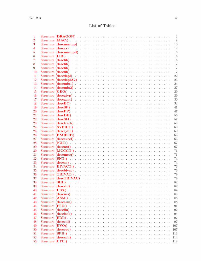
List of Tables

1 Structure (DRAGON) . . . . . . . . . . . . . . . . . . . . . . . . . . . . . . . . . . . . . 32 Structure (MAC:) . . . . . . . . . . . . . . . . . . . . . . . . . . . . . . . . . . . . . . . . 93 Structure (descmacinp) . . . . . . . . . . . . . . . . . . . . . . . . . . . . . . . . . . . . 104 Structure (descxs) . . . . . . . . . . . . . . . . . . . . . . . . . . . . . . . . . . . . . . . . 125 Structure (descmacupd) . . . . . . . . . . . . . . . . . . . . . . . . . . . . . . . . . . . . 156 Structure (LIB:) . . . . . . . . . . . . . . . . . . . . . . . . . . . . . . . . . . . . . . . . . 167 Structure (desclib) . . . . . . . . . . . . . . . . . . . . . . . . . . . . . . . . . . . . . . . 168 Structure (desclib) . . . . . . . . . . . . . . . . . . . . . . . . . . . . . . . . . . . . . . . 179 Structure (desclib) . . . . . . . . . . . . . . . . . . . . . . . . . . . . . . . . . . . . . . . 1710 Structure (desclib) . . . . . . . . . . . . . . . . . . . . . . . . . . . . . . . . . . . . . . . 1711 Structure (descdepl) . . . . . . . . . . . . . . . . . . . . . . . . . . . . . . . . . . . . . . 2212 Structure (descdeplA2) . . . . . . . . . . . . . . . . . . . . . . . . . . . . . . . . . . . . 2313 Structure (descmix1) . . . . . . . . . . . . . . . . . . . . . . . . . . . . . . . . . . . . . . 2414 Structure (descmix2) . . . . . . . . . . . . . . . . . . . . . . . . . . . . . . . . . . . . . . 2715 Structure (GEO:) . . . . . . . . . . . . . . . . . . . . . . . . . . . . . . . . . . . . . . . . 2916 Structure (descgtyp) . . . . . . . . . . . . . . . . . . . . . . . . . . . . . . . . . . . . . . 2917 Structure (descgcnt) . . . . . . . . . . . . . . . . . . . . . . . . . . . . . . . . . . . . . . 3018 Structure (descBC) . . . . . . . . . . . . . . . . . . . . . . . . . . . . . . . . . . . . . . . 3219 Structure (descSP) . . . . . . . . . . . . . . . . . . . . . . . . . . . . . . . . . . . . . . . 4120 Structure (descPP) . . . . . . . . . . . . . . . . . . . . . . . . . . . . . . . . . . . . . . . 4721 Structure (descDH) . . . . . . . . . . . . . . . . . . . . . . . . . . . . . . . . . . . . . . . 5622 Structure (descSIJ) . . . . . . . . . . . . . . . . . . . . . . . . . . . . . . . . . . . . . . . 5723 Structure (desctrack) . . . . . . . . . . . . . . . . . . . . . . . . . . . . . . . . . . . . . . 5924 Structure (SYBILT:) . . . . . . . . . . . . . . . . . . . . . . . . . . . . . . . . . . . . . . 6025 Structure (descsybil) . . . . . . . . . . . . . . . . . . . . . . . . . . . . . . . . . . . . . . 6026 Structure (EXCELT:) . . . . . . . . . . . . . . . . . . . . . . . . . . . . . . . . . . . . . 6327 Structure (descexcel) . . . . . . . . . . . . . . . . . . . . . . . . . . . . . . . . . . . . . . 6328 Structure (NXT:) . . . . . . . . . . . . . . . . . . . . . . . . . . . . . . . . . . . . . . . . 6729 Structure (descnxt) . . . . . . . . . . . . . . . . . . . . . . . . . . . . . . . . . . . . . . . 6730 Structure (MCCGT:) . . . . . . . . . . . . . . . . . . . . . . . . . . . . . . . . . . . . . . 7131 Structure (descmccg) . . . . . . . . . . . . . . . . . . . . . . . . . . . . . . . . . . . . . . 7132 Structure (SNT:) . . . . . . . . . . . . . . . . . . . . . . . . . . . . . . . . . . . . . . . . 7433 Structure (descsn) . . . . . . . . . . . . . . . . . . . . . . . . . . . . . . . . . . . . . . . . 7434 Structure (BIVACT:) . . . . . . . . . . . . . . . . . . . . . . . . . . . . . . . . . . . . . . 7635 Structure (descbivac) . . . . . . . . . . . . . . . . . . . . . . . . . . . . . . . . . . . . . . 7636 Structure (TRIVAT:) . . . . . . . . . . . . . . . . . . . . . . . . . . . . . . . . . . . . . . 7937 Structure (descTRIVAC) . . . . . . . . . . . . . . . . . . . . . . . . . . . . . . . . . . . 7938 Structure (SHI:) . . . . . . . . . . . . . . . . . . . . . . . . . . . . . . . . . . . . . . . . . 8239 Structure (descshi) . . . . . . . . . . . . . . . . . . . . . . . . . . . . . . . . . . . . . . . 8240 Structure (USS:) . . . . . . . . . . . . . . . . . . . . . . . . . . . . . . . . . . . . . . . . . 8441 Structure (descuss) . . . . . . . . . . . . . . . . . . . . . . . . . . . . . . . . . . . . . . . 8542 Structure (ASM:) . . . . . . . . . . . . . . . . . . . . . . . . . . . . . . . . . . . . . . . . 8843 Structure (descasm) . . . . . . . . . . . . . . . . . . . . . . . . . . . . . . . . . . . . . . 8844 Structure (FLU:) . . . . . . . . . . . . . . . . . . . . . . . . . . . . . . . . . . . . . . . . 9145 Structure (descflu) . . . . . . . . . . . . . . . . . . . . . . . . . . . . . . . . . . . . . . . 9246 Structure (descleak) . . . . . . . . . . . . . . . . . . . . . . . . . . . . . . . . . . . . . . 9447 Structure (EDI:) . . . . . . . . . . . . . . . . . . . . . . . . . . . . . . . . . . . . . . . . . 9748 Structure (descedi) . . . . . . . . . . . . . . . . . . . . . . . . . . . . . . . . . . . . . . . 9749 Structure (EVO:) . . . . . . . . . . . . . . . . . . . . . . . . . . . . . . . . . . . . . . . . 10750 Structure (descevo) . . . . . . . . . . . . . . . . . . . . . . . . . . . . . . . . . . . . . . . 10751 Structure (SPH:) . . . . . . . . . . . . . . . . . . . . . . . . . . . . . . . . . . . . . . . . 11352 Structure (descsph) . . . . . . . . . . . . . . . . . . . . . . . . . . . . . . . . . . . . . . . 11453 Structure (CFC:) . . . . . . . . . . . . . . . . . . . . . . . . . . . . . . . . . . . . . . . . 118

IGE–294 x

54 Structure (desccfc) . . . . . . . . . . . . . . . . . . . . . . . . . . . . . . . . . . . . . . . 11955 Structure (INFO:) . . . . . . . . . . . . . . . . . . . . . . . . . . . . . . . . . . . . . . . . 12156 Structure (info) . . . . . . . . . . . . . . . . . . . . . . . . . . . . . . . . . . . . . . . . . 12157 Structure (COMPO:) . . . . . . . . . . . . . . . . . . . . . . . . . . . . . . . . . . . . . . 12558 Structure (compo data1) . . . . . . . . . . . . . . . . . . . . . . . . . . . . . . . . . . . 12659 Structure (compo data2) . . . . . . . . . . . . . . . . . . . . . . . . . . . . . . . . . . . 12960 Structure (compo data3) . . . . . . . . . . . . . . . . . . . . . . . . . . . . . . . . . . . 13061 Structure (compo data4) . . . . . . . . . . . . . . . . . . . . . . . . . . . . . . . . . . . 13062 Structure (TLM:) . . . . . . . . . . . . . . . . . . . . . . . . . . . . . . . . . . . . . . . . 13263 Structure (desctlm) . . . . . . . . . . . . . . . . . . . . . . . . . . . . . . . . . . . . . . . 13264 Structure (M2T:) . . . . . . . . . . . . . . . . . . . . . . . . . . . . . . . . . . . . . . . . 13565 Structure (M2T data) . . . . . . . . . . . . . . . . . . . . . . . . . . . . . . . . . . . . . 13566 Structure (CHAB:) . . . . . . . . . . . . . . . . . . . . . . . . . . . . . . . . . . . . . . . 13767 Structure (CHAB data) . . . . . . . . . . . . . . . . . . . . . . . . . . . . . . . . . . . . 13768 Structure (CPO:) . . . . . . . . . . . . . . . . . . . . . . . . . . . . . . . . . . . . . . . . 13969 Structure (desccpo) . . . . . . . . . . . . . . . . . . . . . . . . . . . . . . . . . . . . . . . 13970 Structure (SAP:) . . . . . . . . . . . . . . . . . . . . . . . . . . . . . . . . . . . . . . . . 14271 Structure (saphyb data1) . . . . . . . . . . . . . . . . . . . . . . . . . . . . . . . . . . . 14372 Structure (saphyb data2) . . . . . . . . . . . . . . . . . . . . . . . . . . . . . . . . . . . 14573 Structure (saphyb data3) . . . . . . . . . . . . . . . . . . . . . . . . . . . . . . . . . . . 14674 Structure (MC:) . . . . . . . . . . . . . . . . . . . . . . . . . . . . . . . . . . . . . . . . . 14875 Structure (MC data) . . . . . . . . . . . . . . . . . . . . . . . . . . . . . . . . . . . . . . 14876 Structure (T:) . . . . . . . . . . . . . . . . . . . . . . . . . . . . . . . . . . . . . . . . . . 15077 Structure (DMAC:) . . . . . . . . . . . . . . . . . . . . . . . . . . . . . . . . . . . . . . . 15178 Structure (DMAC data) . . . . . . . . . . . . . . . . . . . . . . . . . . . . . . . . . . . . 15179 Structure (DREF:) . . . . . . . . . . . . . . . . . . . . . . . . . . . . . . . . . . . . . . . 15380 Structure (SENS:) . . . . . . . . . . . . . . . . . . . . . . . . . . . . . . . . . . . . . . . . 15581 Structure (SENS data) . . . . . . . . . . . . . . . . . . . . . . . . . . . . . . . . . . . . . 15582 Structure (DUO:) . . . . . . . . . . . . . . . . . . . . . . . . . . . . . . . . . . . . . . . . 15783 Structure (DUO data) . . . . . . . . . . . . . . . . . . . . . . . . . . . . . . . . . . . . . 15784 Structure (PSP:) . . . . . . . . . . . . . . . . . . . . . . . . . . . . . . . . . . . . . . . . 16085 Structure (descpsp) . . . . . . . . . . . . . . . . . . . . . . . . . . . . . . . . . . . . . . . 16086 Structure (equality) . . . . . . . . . . . . . . . . . . . . . . . . . . . . . . . . . . . . . . . 16287 Structure (UTL:) . . . . . . . . . . . . . . . . . . . . . . . . . . . . . . . . . . . . . . . . 16388 Structure (DELETE:) . . . . . . . . . . . . . . . . . . . . . . . . . . . . . . . . . . . . . 16589 Structure (BACKUP:) . . . . . . . . . . . . . . . . . . . . . . . . . . . . . . . . . . . . . 16690 Structure (RECOVER:) . . . . . . . . . . . . . . . . . . . . . . . . . . . . . . . . . . . . 16791 Structure (ADD:) . . . . . . . . . . . . . . . . . . . . . . . . . . . . . . . . . . . . . . . . 16892 Structure (MPX:) . . . . . . . . . . . . . . . . . . . . . . . . . . . . . . . . . . . . . . . . 16993 Structure (STAT:) . . . . . . . . . . . . . . . . . . . . . . . . . . . . . . . . . . . . . . . . 17094 Structure (GREP:) . . . . . . . . . . . . . . . . . . . . . . . . . . . . . . . . . . . . . . . 17195 Structure (MSTR:) . . . . . . . . . . . . . . . . . . . . . . . . . . . . . . . . . . . . . . . 17396 Structure (FIND0:) . . . . . . . . . . . . . . . . . . . . . . . . . . . . . . . . . . . . . . . 17597 Structure (ABORT:) . . . . . . . . . . . . . . . . . . . . . . . . . . . . . . . . . . . . . . 17698 Structure (END:) . . . . . . . . . . . . . . . . . . . . . . . . . . . . . . . . . . . . . . . . 17799 Structure (DRVMPI:) . . . . . . . . . . . . . . . . . . . . . . . . . . . . . . . . . . . . . 178100 Structure (SNDMPI:) . . . . . . . . . . . . . . . . . . . . . . . . . . . . . . . . . . . . . 179101 Structure assertS . . . . . . . . . . . . . . . . . . . . . . . . . . . . . . . . . . . . . . . . . 281102 Structure assertV . . . . . . . . . . . . . . . . . . . . . . . . . . . . . . . . . . . . . . . . . 281103 Structure (descmodule) . . . . . . . . . . . . . . . . . . . . . . . . . . . . . . . . . . . . 287104 Structure (descobject) . . . . . . . . . . . . . . . . . . . . . . . . . . . . . . . . . . . . . 288

IGE–294 1

1 INTRODUCTION

The computer code DRAGON is a lattice code designed around solution techniques of the neutrontransport equation.[1] The DRAGON project results from an effort made at Ecole Polytechnique deMontreal to rationalize and unify into a single code the different models and algorithms used in a lat-tice code.[2–5] One of the main concerns was to ensure that the structure of the code was such that thedevelopment and implementation of new calculation techniques would be facilitated. DRAGON is there-fore a lattice cell code which is divided into many calculation modules linked together using the GANgeneralized driver[6, 7]. These modules exchange informations only via well defined data structures.

The two main components of the code DRAGON are its multigroup flux solver and its one-groupcollision probability (CP) tracking modules. The CP modules all perform the same task but usingdifferent levels of approximation.

The SYBIL tracking option emulates the main flux calculation option available in the APOLLO-1 code,[8, 16] and includes a new version of the EURYDICE-2 code which performs reactor assemblycalculations in both rectangular and hexagonal geometries using the interface current method. Theoption is activated when the SYBILT: module is called.

The EXCELL tracking option is used to generate the collision probability matrices for the caseshaving cluster, two-dimensional or three-dimensional mixed rectangular and cylindrical geometries.[18, 19]

A cyclic tracking option is also available for treating specular boundary conditions in two-dimensionalrectangular geometry.[23, 26] EXCELL calculations are performed using the EXCELT: or NXT: module.

The MCCG tracking option activates the long characteristics solution technique. This implementationuses the same tracking as EXCELL and perform flux integration using the long characteristics algorithmproposed by Igor Suslov.[20–22] The option is activated when both EXCELT: (or NXT:) and MCCGT:modulesare called.

After the collision probability or response matrices associated with a given cell have been generated,the multigroup solution module can be activated. This module uses the power iteration method andrequires a number of iteration types.[30] The thermal iterations are carried out by DRAGON so as torebalance the flux distribution only in cases where neutrons undergo up-scattering. The power iterationsare performed by DRAGON to solve the fixed source or eigenvalue problem in the cases where a mul-tiplicative medium is analyzed. The effective multiplication factor (Keff) is obtained during the poweriterations. A search for the critical buckling may be superimposed upon the power iterations so as toforce the multiplication factor to take on a fixed value.[31]

DRAGON can access directly standard microscopic cross-section libraries in various formats. It hasthe capability of exchanging macroscopic cross-section libraries with a code such as TRANSX-CTR orTRANSX-2 by the use of GOXS format files.[32, 35] The macroscopic cross section can also be read inDRAGON via the input data stream.

IGE–294 2

2 GENERAL STRUCTURE OF THE DRAGON INPUT

The input to DRAGON is set up in the form of a structure containing commands which call succes-sively each of the calculation modules required in a given transport calculation.

2.1 Data organization

The structure of the input data is independent of the physical or computational characteristics of thehost system. The physical characteristics of the input data is a collection of sequential records. Thesecharacters are by necessity ascii characters. The logical organization of an input deck is in the form ofa sequential structure of input variables presented in free format. This structure must be located in thefirst 72 columns of each record in the input stream. Characters located in column 73 and above can beused to identify the records and are treated as comments. An input variable can be defined in one of twoways.

• As a set of consecutive characters containing no blanks; it will be considered by DRAGON auto-matically as being an either an integer, a real or a character variable depending on the format ofthe input variable.

• As a set of characters enclosed between quotation marks (’). In this case, the input variable isalways considered to be a character variable.

The only separator allowed between two input variables is a single or a set of blanks (not enclosedbetween quotation marks). A single input variable cannot span two records. Comments can be includedin the input deck in one of the following ways:

• characters in column 73 or above on each record are considered to be comments;

• all the information following the ‘;’ keyword on a record are not considered by the generalizeddriver;

• each record starting with the characters ‘*’ is considered to be commented out;

• all the characters on a given record inserted between ‘(*’ and ‘’*)’ are considered to be commentedout.

This users guide was written using the following conventions:

• An input structure represents a set of input variables. It is identified by a name in boldfacesurrounded by parenthesis. For example, the complete DRAGON input deck is represented by thestructure (DRAGON);

• A standard DRAGON data structure represents a set records and directory stored in a hierarchicalformat on a direct access XSM file or in memory via a linked list.[45] It is identified by a namein small capital letter. For example, the data structure asmpij contains the multigroup collisionprobability matrices generated by the ASM: module of DRAGON;

• The variables presented using the typewriter font are character variables used as keywords. Forexample GEO: is the keyword required to activate the geometry reading module of DRAGON.

• The variables in italics are user defined variables. When indexed and surrounded by parenthesisthey denote arrays. If they are in lower case they represent either integer type (starting withi to n) or real type (starting with a to h or o to z) variables. If they are in upper case theyrepresent character type variables. For example, iprint must be replaced in the input deck by aninteger variable, (energy(igroup), igroup=1,ngroup+1) states that a vector containing ngroup+1real elements is to be read while FILE must be replaced by a character variable, its maximum sizebeing generally specified. No character variable can exceed 72 character in length.

• The variables or structures surrounded by single square brackets ‘[ ]’ are optional.

IGE–294 3

• The variables or structures surrounded by double square brackets ‘[[ ]]’ are also optional. However,they can be repeated as many times as required.

• The variables or structures surrounded by braces and separated by vertical bars ‘ | | ’ representsvarious calculation options available in DRAGON. Only one of these options is permitted.

When a fixed default value is specified for an optional parameter in a structure, it can be modifiedonly locally and is reset to the original default value each time the module is called. When a floatingdefault value is specified for a variable, it is saved and can be used in later calls to this module. InDRAGON, almost every default value is a floating value, with the exception of the parameter iprint,which is set to 1 and is used to control the amount of information printed in the module. Departure fromthis general rule will be indicated in the following sections.

2.2 DRAGON Data Structure and Module Declarations

DRAGON is built around the GAN generalized driver.[6] Accordingly, all the modules that will beused during the current execution must be first identified. One must also define the format of each datastructure that will be processed by these modules. Then, the modules required for the specific DRAGONcalculation are called successively, information being transferred from one module to the next via the datastructures. Finally, the execution of DRAGON is terminated when it encounters the END: module evenif it is followed by additional data records in the input data stream. The general input data structuretherefore follows the calling specifications given below:

Table 1: Structure (DRAGON)

[ MODULE [[ MODNAME ]] ; ][ LINKED LIST [[ STRNAME ]] ; ][ XSM FILE [[ STRNAME ]] ; ][ SEQ BINARY [[ STRNAME ]] ; ][ SEQ ASCII [[ STRNAME ]] ; ][[ (module) ; ]]END: ;

where

MODULE keyword used to specify the list of modules to be used in this DRAGON execution.

MODNAME character*12 name of a DRAGON or utility module. The list of DRAGON moduleis provided in Section 2.3 while the list of Utility module is described in Section 2.4.By default a ‘ ’ module is always available (see Sections 2.4 and 4.1).

LINKED LIST keyword used to specify which data structures will be stored in linked lists.

XSM FILE keyword used to specify which data structures will be stored on XSM format files.

SEQ BINARY keyword used to specify which data structures will be stored on sequential binary files.

SEQ ASCII keyword used to specify which data structures will be stored on sequential ASCII files.

STRNAME character*12 name of a DRAGON data structure. Note that on MVS file names aretruncated to 7 characters due to a constraint of this operating system. The list ofDRAGON data structure is presented in Section 2.5.

(module) input specifications for a DRAGON or utility module. For the DRAGON specificmodules these input structures will be defined in Section 3. For utility modules, therequired structures are described in Section 4.

IGE–294 4

END: keyword to call the normal end-of-execution utility module.

; end of record keyword. This keyword is used by DRAGON to delimit the part of theinput data stream associated with each module.

Note that the user generally has the choice to declare most of the data structures in the format of alinked list to reduce CPU times or as a XSM file to reduce memory resources. Some exceptions to thisgeneral rule are the tracking files as we will see in Section 3.4. In general, the data structure are storedon the sequential ASCII files only for backup purposes.

The input data normally ends with a call to the END: module (see Section 4.13). However, the GANdriver will insert automatically the END: module, even if it was not provided, upon reaching an end-of-filein the input stream.

Each (module) specification contains a description of the execution modules to be called and itsassociated input structure. All these modules, except the END: module may be called more than once.

2.3 The DRAGON Modules

The code DRAGON has been divided into main calculations sequences to which is generally associateda single calculation module. The only exception to this rule is the tracking sequence to which is associatedmany different modules, one for each of the standard CP calculation options and an additional modulefor diffusion calculations. However, this later module can only be used indirectly in the edition moduleof DRAGON. These modules perform the following tasks:

MAC: module used to generate or modify a DRAGON macrolib (see Section 2.5) whichcontains the group ordered macroscopic cross sections for a series of mixture (seeSection 3.1). This macrolib can be either an independent data structure or it can beincluded as a substructure in a microlib. The spatial location of these mixtures willbe defined using the GEO: module (see Section 3.3).

LIB: module used to generate or modify a DRAGON microlib (see Section 2.5) that canread a number of different types of microscopic cross-section libraries (see Section 3.2).Each such access requires a double interpolation (temperature, dilution) carried outby a subroutine specifically tailored to each type of library. Currently the formatsDRAGLIB[45], WIMS–D4[34], MATXS[32], WIMS–AECL[33], APOLLO[8, 9] and NDASformat[10] are supported. After having reconstructed the microscopic cross sections foreach isotope, they are then multiplied by the isotopic concentrations (particles per cm3)and combined in such a way as to produce an embedded macrolib (see Section 2.5).The spatial location of these mixtures will be defined using the GEO: module (seeSection 3.3).

GEO: module used to generate or modify a geometry (see Section 3.3).

SYBILT: the standard tracking module based on 1D collision probability or Interface Currenttechnique (see Section 3.4 and Section 3.4.1).

EXCELT: the standard tracking module for 2D and 3D geometries as well as isolated 2D cellscontaining clusters (see Section 3.4 and Section 3.4.2).

NXT: the standard tracking module for 2D or 3D assemblies of cluster (see Section 3.4 andSection 3.4.3).

SNT: the discrete ordinates tracking module (see Section 3.4 and Section 3.4.5).

MCCGT: the tracking module of the open characteristics flux solver (see Section 3.4 and Sec-tion 3.4.4).

BIVACT: the 1D/2D diffusion and SPn tracking module (see Section 3.4 and Section 3.4.6).

TRIVAT: the 1D/2D/3D diffusion and SPn tracking module (see Section 3.4 and Section 3.4.7).

IGE–294 5

SHI: module used to perform self-shielding calculations using the generalized Stamm’lermethod (see Section 3.5).

USS: module used to perform self-shielding calculations using a subgroup method (see Sec-tion 3.6). A method using physical probability tables (cf. Wims-7 and Helios) and theRibon extended method are available.

ASM: module which uses the tracking information to generate a multigroup response orcollision probability matrix (see Section 3.7).

FLU: module which uses inner-iteration approach or collision probability matrix to solvethe transport equation for the fluxes (see Section 3.8). Various leakage models areavailable.

EDI: editing module (see Section 3.9). An equivalence method based on SPH method isavailable.

EVO: burnup module (see Section 3.10).

SPH: supermomogeneisation (SPH) module (see Section 3.11). The SPH: module can alsobe used to extract a microlib or macrolib from a multicompo or saphyb.

INFO: utility to compute number densities for selected isotopes in materials such as UO2 orThUO2 (see Section 3.13).

COMPO: multi-parameter reactor database construction module (see Section 3.14).

TLM: module used to generate a Matlab M-file to obtain a graphics representation of theNXT: tracking lines (see Section 3.15).

M2T: interface module for transforming a macrolib into a Trimaran/Tripoli multigroup file(see Section 3.16).

CHAB: cross section perturbation module similar to CHABINT (see Section 3.17).

CPO: burnup-dependent mono-parameter reactor database construction module (see Sec-tion 3.18).

SAP: multi-parameter reactor database construction module in SAPHYB format (see Sec-tion 3.19).

MC: multigroup Monte-Carlo flux solution module (see Section 3.20).

T: macrolib transposition operator (see Section 3.21).

DMAC: construction module for a Generalized Perturbation Theory (GPT) source (see Sec-tion 3.22).

SENS: sensitivity analysis of keff to nuclear data (see Section 3.24).

PSP: module to generate PostScript images for 2D geometries that can be tracked using themodule EXCELT: or NXT: (see Section 3.26).

DUO: module to perform a perturbative analysis of two systems using the Clio formula andto determine the origins of Keff discrepancies (see Section 3.25).

IGE–294 6

2.4 The Utility Modules

Because the execution of DRAGON is controlled by the GAN generalized driver it can use directlyany one of its utility modules. These modules perform the following tasks:

’ ’ default module used to make an explicit copy of a data structure (see Section 4.1).

UTL: module used to manipulate a data structure (see Section 4.2).

DELETE: module used to delete a data structure (see Section 4.3).

BACKUP: module used to make a backup copy of a child data structure along with its parent(see Section 4.4).

RECOVER: module used to recover form a backup copy a child data structure along with its parent(see Section 4.5).

ADD: module used to add two data structures (see Section 4.6).

MPX: module used to multiply a data structure by a constant (see Section 4.7).

STAT: module used to compare two data structures (see Section 4.8).

GREP: module used to locate information on a data structure (see Section 4.9).

FIND0: module used to find the zero of a tabulated function (see Section 4.11).

END: module used to terminate an execution controlled by the generalized driver (see Sec-tion 4.13).

2.5 The DRAGON Data Structures

The transfer of information between the DRAGON execution modules is ensured by well defined datastructure. They are generally created or modified directly by one of the modules of DRAGON or by oneof the utility modules. Here we will give a brief description of these data structures but a more completedescription of their content is also available upon request.[45] These data structures are memory-residentor persistent (i.e., XSM–type) objects.

macrolib a standard data structure used by DRAGON to transfer group-ordered macroscopiccross sections between its modules. It can be a stand-alone structure or it can beincluded into a larger structure, such as a microlib or an edition structure. It canbe created by the MAC:, LIB: and EDI: modules. It can also be modified by the SHI:,USS: and EVO:modules. Such a structure (either stand-alone or as part of a microlib)is also required for a successful execution of the ASM: and FLU: modules.

microlib a standard data structure used by DRAGON to transfer microscopic and macroscopiccross sections between its modules. It always include a macrolib substructure. Itcan be a stand-alone structure or included into a larger structure, such as an edition

structure. It can be created by the LIB: and EDI: modules. It can also be modifiedby the MAC:, SHI:, USS: and EVO: modules.

geometry a standard data structure used by DRAGON to transfer the geometry between itsmodules. It can be a stand-alone structure or included into a larger structure, such asanother geometry structure. It can be created by the GEO: module. Such a structureis also required directly for a successful execution of the tracking modules (SYBILT:,EXCELT: and MCCGT:).

tracking a standard data structure used by DRAGON to transfer the general tracking infor-mation between its modules. It is a stand-alone structure. It can be created by theSYBILT:, EXCELT: and MCCGT: modules. Such a structure is also required directly fora successful execution of the ASM: module.

IGE–294 7

asmpij a standard data structure used by DRAGON to transfer the multigroup response andcollision probability matrices between its modules. It is a stand-alone structure. It iscreated by the ASM: module. Such a structure is also required directly for a successfulexecution of the FLU: module.

fluxunk a standard data structure used by DRAGON to transfer the fluxes between its modules.It is a stand-alone structure. It is created by the FLU: module. Such a structure isalso required for a successful execution of the EDI: and EVO: modules.

edition a standard data structure used by DRAGON to store condensed and merged micro-scopic and macroscopic cross sections. It is a stand-alone structure but can containmacrolib and microlib substructure. It is created by the EDI: module. Such astructure is also required for a successful execution of the COMPO: module.

burnup a standard data structure used by DRAGON to store burnup informations. It is createdby the EVO: module. Such a structure is also required for a successful execution of theCOMPO: module.

draglib a standard data structure used by DRAGON (input) to recover isotopic–, dilution– andtemperature–dependent information, including multigroup microscopic cross sectionsand burnup data. This is a stand-alone structure that is generally stored on a persistentLCM object. It may be created by the dragr module of NJOY.

cpo a standard data structure used by DRAGON to store a simplified reactor dabase. Itis a stand-alone structure that must be stored on a linked list or an XSM file. Itis created by the CPO: module. It is required for a successful execution of the CFC:

module. It can be used by the CRE: module of DONJON.

multicompo a standard data structure used by DRAGON (output) to store reactor related in-formation and to classified it using tuples of local and global parameters. This is astand-alone structure that is generally stored on a persistent LCM object. It is createdby the COMPO: module.

saphyb a standard data structure used by APOLLO2 and DRAGON (output) to store reactorrelated information and to classified it using tuples of global parameters. This is astand-alone structure that is generally stored on a persistent LCM object. It is createdby the SAP: module.

fbmxsdb a standard data structure used by DRAGON to store a full reactor cross sectiondatabase with Feedback coefficients. It is a stand-alone structure that must be storedon a linked list or an XSM file. It is created by the CFC: module. It can be used bythe AFM: module of DONJON.[88]

2.6 Main Updates in DRAGON

The frozen version (DRAGON Release 3.06) has seen a large number of changes since the first officialrelease of the code (DRAGON 960627).

The current DRAGON package (DRAGON Version4) is an evolution of the frozen version, releasedas an attempt to introduce innovative capabilities:

• The new self-shielding module USS: allow increased accuracy and better representation of phenom-ena such as distributed self-shielding effects and mutual self-shielding effects.

• The new flux solution solver MCCG is an implementation of the long characteristics method pro-posed by Igor Suslov. This solver is initiated by the new tracking module MCCGT:.

• The new flux solution module FLU: is a complete rewrite of the outer iteration for the multigroupflux calculation that is now compatible with the method of characteristics and with any otherapproach requiring inner iterations. The MOCC: module is no longer required.

IGE–294 8

• The burnup module EVO: was extended to take into account energy produced by radioactive decayand by reactions other than fission.

• The new module COMPO: is used to create and increment a multiparameter reactor database. Themodule The companion module NCR: is used to interpolate an existing multiparameter reactordatabase.

• The flux solution solver SYBIL related to 2D assembly calculations was extended to allow sector-ization of the cells.

• The method of discrete ordinates is implemented in tracking module SNT:.

• The EXCELL: module has been removed, but its capability is now implemented using the XCLL

keyword in EXCELT:.

• The LIB: module can access NDAS-formatted cross-section libraries.

IGE–294 9

3 THE DRAGON MODULES

The input to DRAGON is set up in the form of a structure containing commands which call succes-sively each of the calculation modules required in a given transport calculation.

3.1 The MAC: module

In DRAGON, the macroscopic cross sections associated with each mixture are stored in a macrolib

(as an independent data structure or as part of a microlib) which may be generated using one of differentways:

• First, one can use directly the input stream already used for the remaining DRAGON data. In thiscase, a single macroscopic library is involved.

• The second method is via a GOXS format binary sequential file.[32] It should be noted that a numberof GOXS files may be read successively by DRAGON and that it is possible to combine data fromGOXS files with data taken from the input stream. One can also transfer the macroscopic crosssections to a GOXS format binary file if required. In this case, a single macroscopic library isinvolved.

• The third input method is through a file which already contains a macrolib. In this case, twomacroscopic and microscopic libraries are to be combined

• The fourth method consists to update an existing macrolib using control-variable data recoveredfrom a L OPTIMIZE object.

The general format of the data for the MAC: module is the following:

Table 2: Structure (MAC:)

MACLIB := MAC: [ MACLIB ] :: (descmacinp)| MICLIB := MAC: MICLIB :: (descmacinp)| MACLIB := MAC: [ MACLIB ] [ OLDLIB ] :: (descmacupd)| MACLIB := MAC: MACLIB OPTIM ;

The meaning of each of the terms above is:

MACLIB character*12 name of a macrolib that will contain the macroscopic cross sections.If MACLIB appears on both LHS and RHS, it is updated; otherwise, it is created. IfMACLIB is created, all macroscopic cross sections are first initialized to zero.

MICLIB character*12 name of a microlib. Only the macrolib data substructure of thismicrolib is then updated. This is used mainly to associate fixed sources densitieswith various mixtures. If any other cross section is modified for a specific mixture, themicroscopic and macroscopic cross sections are no longer compatible. One can returnto a compatible library using the library update module (see Section 3.2).

OLDLIB character*12 name of a macrolib or a microlib which will be used to update orcreate the MACLIB macrolib.

OPTIM character*12 name of a L OPTIMIZE object. The macrolib MACLIB is updatedusing control-variable data recovered from OPTIM .

(descmacinp) macroscopic input data structure for this module (see Section 3.1.1).

IGE–294 10

(descmacupd) macroscopic update data structure for this module (see Section 3.1.3).

3.1.1 Input structure for module MAC:

In the case where there are no OLDLIB specified, the (descmac) input structure takes the form:

Table 3: Structure (descmacinp)

[ EDIT iprint ][ NGRO ngroup ][ NMIX nmixt ][ NIFI nifiss ][ DELP ndel ][ ANIS naniso ][ CTRA NONE | APOL | WIMS | LEAK ][ NALP nalbp ][ ALBP (albedp(ia),ia=1,nalbp) ][ WRIT GOXSWN ][ ENER (energy(jg), jg=1,ngroup +1) ][ VOLUME (volume(ibm), ibm=1,nmixt) ][ ADD ][[ READ [ (imat(i), i=1,nmixt) ] GOXSRN [ DELE ] | READ INPUT [[ (descxs) ]] ]][[ STEP istep READ INPUT [[ (descxs) ]] ]][ NORM ];

with

EDIT keyword used to modify the print level iprint.

iprint index used to control the printing in this module. It must be set to 0 if no printing onthe output file is required. The macroscopic cross sections can written to the outputfile if the variable iprint is greater than or equal to 2. The transfer cross sections willbe printed if this parameter is greater than or equal to 3. The normalization of thetransfer cross sections will be checked if iprint is greater than or equal to 5.

NGRO keyword to specify the number of energy groups for which the macroscopic cross sec-tions will be provided. This information is required only if MACLIB is created andthe cross sections are taken directly from the input data stream.

ngroup the number of energy groups used for the calculations in DRAGON. The default valueis ngroup=1.

NMIX keyword used to define the number of material mixtures. This information is requiredonly if MACLIB is created and the cross sections are taken directly from the inputdata stream or from a GOXS file.

nmixt the maximum number of mixtures (a mixture is characterized by a distinct set ofmacroscopic cross sections) the macrolib may contain. The default value is nmixt=1.

NIFI keyword used to specify the maximum number of fissile spectrum associated with eachmixture. Each fission spectrum generally represents a fissile isotope. This information

IGE–294 11

is required only if MACLIB is created and the cross sections are taken directly fromthe input data stream.

nifiss the maximum number of fissile isotopes per mixture. The default value is nifiss=1.

DELP keyword used to specify the number of delayed neutron groups.

ndel the number of delayed neutron groups. The default value is ndel=0.

ANIS keyword used to specify the maximum level of anisotropy permitted in the scatteringcross sections. This information is required only if MACLIB is created and the crosssections are taken directly from the input data stream.

naniso number of Legendre orders for the representation of the scattering cross sections. Thedefault value is naniso=1 corresponding to the use of isotropic scattering cross sections.

CTRA keyword to specify the type of transport correction that should be generated and storedon the macrolib. The transport correction is to be substracted from the total andisotropic (P0) within-group scattering cross sections. A leakage correction, equal tothe difference between current– and flux–weighted total cross sections (Σ1−Σ0) is alsoapplied in the APOL and LEAK cases. All the modules that will read this macrolib

will then have access to transport corrected cross sections. The default is no transportcorrection when the macrolib is created from the input or GOXS files.

NONE keyword to specify that no transport correction should be used in this calculation.

APOL keyword to specify that an APOLLO type transport correction based on the linearlyanisotropic (P1) scattering cross sections is to be set. This correction assumes that themicro-reversibility principle is valid for all energy groups. P1 scattering informationmust exists in the macrolib.

WIMS keyword to specify that a WIMS–type transport correction is used. The transportcorrection is recovered from a record named TRANC. This record must exists in themacrolib.

LEAK A leakage correction is applied to the total and P0 within-group scattering cross sec-tions. No transport correction is applied in this case.

NALP keyword to specify the maximum number of physical albedos which will be read. Thesecan be used by the GEO: module (see Section 3.3).

nalbp the maximum number of physical albedos. The default value is nalbp=1.

ALBP keyword used for the input of the physical albedo array.

albedp physical albedo array. A maximum of nalbp entries can be specified.

WRIT keyword used to write cross section data to a GOXS file. In the case where nifiss>1,this option is invalid.

GOXSWN character*7 name of the GOXS file to be created or updated.

ENER keyword to specify the energy group limits.

energy energy (eV) array which define the limits of the groups (ngroup+1 elements). Gener-ally energy(1) is the highest energy.

VOLUME keyword to specify the mixture volumes.

volume volume (cm3) occupied by each mixture.

ADD keyword for adding increments to existing macroscopic cross sections. In this case, theinformation provided in (descxs) represents incremental rather than standard crosssections.

IGE–294 12

READ keyword to specify the input file format. One can use either the input stream (keywordINPUT) or a GOXS format file.

imat array of mixture identifiers to be read from a GOXS file. The maximum number ofidentifiers permitted is nmixt and the maximum value that imat may take is nmixt.When imat is 0, the corresponding mixture on the GOXS file is not included in themacrolib. In the cases where imat is absent all the mixtures on the GOXS file areavailable in a DRAGON execution. They are numbered consecutively starting at 1 orfrom the last number reached during a previous execution of the MAC: module.

GOXSRN character*7 name of the GOXS file to be read.

DELE keyword to specify that the GOXS file is deleted after being read (Revision 3.03only).

INPUT keyword to specify that mixture cross sections will be read on the input stream.

(descxs) structure describing the format used for reading the mixture cross sections from theinput stream (see Section 3.1.2).

STEP keyword used to create a perturbation directory.

istep the index of the perturbation directory.

NORM keyword to specify that the macroscopic scattering cross sections and the fission spec-trum have to be normalized. This option is available even if the mixture cross sectionswere not read by the MAC: module.

3.1.2 Macroscopic cross section definition

Table 4: Structure (descxs)

MIX [ matnum ][ NTOT0 | TOTAL (xssigt(jg), jg=1,ngroup) ][ NTOT1 (xssig1(jg), jg=1,ngroup) ][ TRANC (xsstra(jg), jg=1,ngroup) ][ NUSIGF ((xssigf (jf,jg), jg=1,ngroup), jf=1,nifiss) ][ CHI ((xschi(jf,jg), jg=1,ngroup), jf=1,nifiss)][ FIXE (xsfixe(jg), jg=1,ngroup) ][ DIFF (diff (jg), jg=1,ngroup) ][ DIFFX (xdiffx(jg), jg=1,ngroup) ][ DIFFY (xdiffy(jg), jg=1,ngroup) ][ DIFFZ (xdiffz(jg), jg=1,ngroup) ][ NUSIGD (((xssigd(jf,idel,jg), jg=1,ngroup), idel=1,ndel), jf=1,nifiss) ][ CHDL (((xschid(jf,idel,jg), jg=1,ngroup), idel=1,ndel), jf=1,nifiss)][ OVERV (overv(jg), jg=1,ngroup) ][ NFTOT (nftot(jg), jg=1,ngroup) ][ FLUX-INTG (xsint0(jg), jg=1,ngroup) ][ FLUX-INTG-P1 (xsint1(jg), jg=1,ngroup) ][ H-FACTOR (hfact(jg), jg=1,ngroup) ][ SCAT (( nbscat(jl,jg), ilastg(jl,jg),(xsscat(jl,jg,ig),

ig=1,nbscat(jl,jg) ), jg=1,ngroup), jl=1,naniso) ]

IGE–294 13

MIX keyword to specify that the macroscopic cross sections associated with a new mixtureare to be read.

matnum identifier for the next mixture to be read. The maximum value permitted for thisidentifier is nmixt. When matnum is absent, the mixtures are numbered consecutivelystarting with 1 or with the last mixture number read either on the GOXS or the inputstream.

NTOT0 keyword to specify that the total macroscopic cross sections for this mixture follows.

TOTAL alias keyword for NTOT0.

xssigt array representing the multigroup total macroscopic cross section (Σg in cm−1) asso-ciated with this mixture.

NTOT1 keyword to specify that the P1–weighted total macroscopic cross sections for this mix-ture follows.

xssig1 array representing the multigroup P1–weighted total macroscopic cross section (Σg1 in

cm−1) associated with this mixture.

TRANC keyword to specify that the transport correction macroscopic cross sections for thismixture follows.

xsstra array representing the multigroup transport correction macroscopic cross section (Σgtc

in cm−1) associated with this mixture.

NUSIGF keyword to specify that the macroscopic fission cross section multiplied by the averagenumber of neutrons per fission for this mixture follows.

xssigf array representing the multigroup macroscopic fission cross section multiplied by theaverage number of neutrons per fission (νΣg

f in cm−1) for all the fissile isotopes asso-ciated with this mixture.

CHI keyword to specify that the fission spectrum for this mixture follows.

xschi array representing the multigroup fission spectrum (χg) for all the fissile isotopes as-sociated with this mixture.

FIXE keyword to specify that the fixed neutron source density for this mixture follows.

xsfixe array representing the multigroup fixed neutron source density for this mixture (Sg ins−1cm−3).

DIFF keyword to specify that the isotropic diffusion coefficient for this mixture follows.

diff array representing the multigroup isotropic diffusion coefficient for this mixture (Dg

in cm).

DIFFX keyword for input of the X–directed diffusion coefficient.

xdiffx array representing the multigroup X–directed diffusion coefficient (Dgx in cm) for the

mixture matnum.

DIFFY keyword for input of the Y –directed diffusion coefficient.

xdiffy array representing the multigroup Y –directed diffusion coefficient (Dgy in cm) for the

mixture matnum.

DIFFZ keyword for input of the Z–directed diffusion coefficient.

xdiffz array representing the multigroup Z–directed diffusion coefficient (Dgz in cm) for the

mixture matnum.

IGE–294 14

NUSIGD keyword to specify that the delayed macroscopic fission cross section multiplied by theaverage number of neutrons per fission for this mixture follows.

xssigd array representing the delayed multigroup macroscopic fission cross section multipliedby the average number of neutrons per fission (νΣg,idel

f in cm−1) for all the fissileisotopes associated with this mixture.

CHDL keyword to specify that the delayed fission spectrum for this mixture follows.

xschid array representing the delayed multigroup fission spectrum (χg,idel) for all the fissileisotopes associated with this mixture.

OVERV keyword for input of the multigroup average of the inverse neutron velocity.

overv array representing the multigroup average of the inverse neutron velocity (< 1/v >gm)

for the mixture matnum.

NFTOT keyword for input of the multigroup macroscopic fission cross sections.

nftot array representing the multigroup macroscopic fission cross section (Σgf ) for the mix-

ture matnum.

FLUX-INTG keyword for input of the multigroup P0 volume-integrated fluxes.

xsint0 array representing the multigroup P0 volume-integrated fluxes (V φg0) for the mixture

matnum.

FLUX-INTG-P1 keyword for input of the multigroup P1 volume-integrated fluxes.

xsint1 array representing the multigroup P1 volume-integrated fluxes (V φg1) for the mixture

matnum.

H-FACTOR keyword to specify that the power factor for this mixture follows.

hfact array representing the multigroup power factor for this mixture (Hg in MeV cm−1).

SCAT keyword to specify that the macroscopic scattering cross section matrix for this mixturefollows.

nbscat array representing the number of primary groups ig with non vanishing macroscopicscattering cross section towards the secondary group jg considered for each anisotropylevel associated with this mixture.

ilastg array representing the group index of the most thermal group with non-vanishingmacroscopic scattering cross section towards the secondary group jg considered foreach anisotropy level associated with this mixture.

xsscat array representing the multigroup macroscopic scattering cross section (Σig→jgsl in

cm−1) from the primary group ig towards the secondary group jg considered for eachanisotropy level associated with this mixture. The elements are ordered using decreas-ing primary group number ig, from ilastg to (ilastg−nbscat+1), and an increasingsecondary group number jg. Examples of input structures for macroscopic scatteringcross sections can be found in Section 6.1.

3.1.3 Update structure for operator MAC:

In the case where OLDLIB is specified, the (descmacupd) input structure takes the form:

IGE–294 15

Table 5: Structure (descmacupd)

[ EDIT iprint ][ CTRA OFF ][[ MIX numnew [ numold UPDL | OLDL ] ]];

with


iprint index used to control the printing in this operator. It must be set to 0 if no printing onthe output file is required. The macroscopic cross sections can written to the output file ifthe variable iprint is greater than or equal to 2. The transfer cross sections will be printedif this parameter is greater than or equal to 3. The normalization of the transfer crosssections will be checked if iprint is greater than or equal to 5.

CTRA keyword to specify the type of transport correction that should be generated and storedon the macrolib. All the operators that will read this macrolib will then have access totransport corrected cross sections. In the case where the macrolib is updated using othermacrolib or microlib the default is to use a transport correction whenever one of theseolder data structure requires a transport correction.

OFF deactivates the transport correction.

MIX keyword to specify that the macroscopic cross sections associated with a mixture is to becreated or updated.

numnew mixture number to be updated or created on the output macrolib.

numold mixture number on an old macrolib or microlib which will be used to update or createnumnew on the output macrolib

OLDL the macroscopic cross sections associated with mixture numold are taken from OLDLIB.This is the default option.

UPDL the macroscopic cross sections associated with mixture numold are taken from MACLIB.

IGE–294 16

3.2 The LIB: module

The general format of the input data for the LIB: module is the following:

Table 6: Structure (LIB:)

MICLIB := LIB: [ MICLIB [ OLDLIB ] ] :: (desclib)

where

MICLIB character*12 name of the microlib that will contain the internal library. If MICLIBappears on both LHS and RHS, it is updated; otherwise, it is created.

OLDLIB character*12 name of a read-only macrolib, microlib or burnup data structure.In the case where a macrolib is considered, it is included directly in the MICLIBbefore updating it. If it is a second microlib or a burnup data structure, the numberdensities for the isotopes in file MICLIB will be replaced selectively by those found inOLDLIB.

(desclib) input structure for this module (see Section 3.2.1).

3.2.1 Data input for module LIB:

In the case where OLDLIB is absent or represents a macrolib, (desclib) takes the form:

Table 7: Structure (desclib)

[ EDIT iprint ][ NGRO ngroup ][ MXIS nmisot ][ NMIX nmixt ][ CALENDF ipreci ][ CTRA NONE | APOL | WIMS | OLDW | LEAK ] [ ANIS naniso ][ ADJ ][ PROM ][ SKIP | INTR | SUBG | PT | PTMC | PTSL | NEWL ] [ MACR ][ ADED nedit ( HEDIT(i), i=1,nedit ) ][ DEPL LIB: DRAGON | WIMS | WIMSD4 | WIMSAECL | NDAS FIL: NAMEFIL

| LIB: APLIB2 | APXSM FIL: NAMEFIL (descdeplA2)| ndepl (descdepl) ]

[[ MIXS LIB:

DRAGON | MATXS | MATXS2 | WIMS | WIMSD4 | WIMSAECL | NDAS | APLIB1 | APLIB2 | APXSM FIL: NAMEFIL [[ (descmix1) ]] ]]

It is possible to reset an existing microlib (i.e., MICLIB is present in the RHS) and to reprocess all theisotopes from the cross section libraries. In this case, (desclib) takes the simplified form:

IGE–294 17


[ EDIT iprint ] INTR | SUBG | PT | PTMC | PTSL | NEWL [ MACR ]MIXS ;

Alternatively if OLDLIB is absent or represents a second microlib, (desclib) takes the form:


[ EDIT iprint ]MAXS [[ (descmix2) ]]

Finally, if OLDLIB represents burnup structure, (desclib) takes the form:


[ EDIT iprint ]BURN iburn | tburn [[ (descmix2) ]]

with


iprint index used to control the printing in this operator. It must be set to 0 if no printing onthe output file is required while values >0 will increase in steps the amount of informationtransferred to the output file. If iprint≥10, the depletion chain is printed in the formatof structure (descdepl). If iprint≥20, the depletion chain is also printed in the format ofstructure (descdeplA2).

MXIS keyword used to redefine the maximum number of isotopes per mixture.

nmisot the maximum number of isotopes per mixture. By default up to 300 different isotopes permixture are permitted.

NMIX keyword used to define the number of material mixtures. This data is required if MICLIBis created.

nmixt the maximum number of mixtures (a mixture is characterized by a distinct set of macro-scopic cross sections).

CALENDF keyword to set the accuracy of the CALENDF probability tables.

ipreci integer set to 1, 2, 3 or 4. The highest the value, the more accurate are the probabilitytables.

CTRA keyword to specify the type of transport correction that should be generated and stored onthe microlib. The transport correction is to be substracted from the total and isotropic

IGE–294 18

(P0) within-group scattering cross sections. A leakage correction, equal to the differencebetween current– and flux–weighted total cross sections (σ1 − σ0) is also applied in theAPOL, OLDW and LEAK cases. All the operators that will read this microlib will then haveaccess to transport corrected cross sections. The default is no transport correction.

NONE keyword to specify that no transport correction should be used in this calculation.

APOL keyword to specify that an APOLLO type transport correction based on the linearlyanisotropic (P1) within-group scattering cross sections is to be set. This correction as-sumes that the micro-reversibility principle is valid for all energy groups. This type ofcorrection uses P1 scattering information present on the library.

WIMS This type of correction uses directly a transport-correction provided on the library. Suchinformation is available in WIMSD4 and WIMS–AECL libraries. This is the new recom-mended option with WIMS-type libraries. This option has no effect on libraries that doesnot contain transport correction information.

OLDW keyword to specify that a WIMS type transport correction based on the P1 scattering crosssections is to be set. This correction assumes that the micro-reversibility principle is validonly for groups energies less than 4.0 eV. For the remaining groups a 1/E current spectrumis considered in the evaluation of the transport correction. This type of correction uses P1

scattering information present on the library.

LEAK A leakage correction is applied to the total and P0 within-group scattering cross sections.No transport correction is applied in this case.

ANIS keyword to specify the maximum level of anisotropy for the scattering cross sections.

naniso number of Legendre orders for the representation of the scattering cross sections. Isotropicscattering is represented by naniso=1 while naniso=2 represents linearly anisotropic scat-tering. Generally the linearly anisotropic (P1) scattering contributions are taken into ac-count via the transport correction (see CTRA keyword) in the transport calculation. For B1

or P1 leakage calculations, the linearly anisotropic scattering cross sections are taken intoaccount explicitly. The default value is naniso=2.

ADJ keyword to specify the production of adjoint macroscopic cross sections. By default, directcross sections are produced.

PROM keyword to specify that prompt neutrons are to be considered for the calculation of thefission spectrum. By default, the contribution due to delayed neutrons is considered. Thisoption is only compatible with a MATXS or MATXS2 format library.

SKIP keyword to recover the user–defined microlib data without processing any library (i.e.,without temperature and/or dilution interpolation).

INTR keyword to perform a temperature and dilution interpolation of the microscopic crosssections present in the libraries. The bin-type cross-section data is not processed. This isthe default option.

SUBG keyword to activate the calculation of the physical probability tables using the tempera-ture-interpolated cross-section data as input.[11, 13] The bin-type cross-section data is notprocessed.

PT keyword to activate the calculation of the CALENDF-type mathematical probability tables(without slowing-down correlated weight matrices) using the bin-type cross-section dataas input.[12] This option is compatible with the Sanchez-Coste self-shielding method andwith the subgroup projection method (SPM).[14]

PTMC this option is similar to the PT procedure. Here, the base points of the probability tablescorresponding to fission and scattering cross sections and to components of the transferscattering matrix are also obtained using the CALENDF approach.

IGE–294 19

PTSL keyword to activate the calculation of the CALENDF-type mathematical probability ta-bles and slowing-down correlated weight matrices using the bin-type cross-section data asinput.[13]

NEWL keyword to activate the calculation of a DRAGLIB library using the temperature-interpo-lated cross-section data as input. The bin-type cross-section data is processed.

MACR keyword to force the calculation of the embedded macrolib. By default, the embeddedmacrolib is computed, except if one of the key words SKIP, INTR, SUBG, PT or NEWL is used.

ADED keyword to specify the input of additional cross sections to be treated by DRAGON. Thesecross sections are not needed to solve the transport equation but are recognized by theEDI: and utility operators.

nedit number of types of additional cross sections.

HEDIT character*6 name of an additional cross-section type. This name also corresponds tovectorial reactions in a MATXS and MATXS2 format library. For example:

NWT0/NWT1=P0/P1 library weight functions.NTOT0/NTOT1=P0/P1 neutron total cross sections.NELAS=Neutron elastic scattering cross sections (MT=2).NINEL=Neutron inelastic scattering cross sections (MT=4).NG=Neutron radiative capture cross sections (MT=102).NFTOT=Total fission cross sections (MT=18).NUDEL=Number of delayed secondary neutrons (Nu-D / MT=455).NFSLO=ν∗slow fission cross section.NHEAT=Heat production cross section.CHIS/CHID=Slow/delayed fission spectrum.NF/NNF/N2NF/N3NF=ν∗partial fission cross sections (MT=19, 20, 21 and 38).N2N/N3N/N4N=(n,2n), (n,3n), (n,4n) cross sections (MT=16, 17 and 37).NP/NA=(n,p) and (n,α) transmutation cross sections (MT=103 and 107).

By default, DRAGON will always attempt to recover the additional cross sections NG,NFTOT, NHEAT and N2N which are required for the depletion calculations.

DEPL keyword to specify that the isotopic depletion (burnup) chain is to be read. For a givenLIB: execution only one isotopic depletion chain can be read.

MIXS keyword to specify that the mixture description is to be read. For a given LIB: executionmore than one cross-section library can be read.

LIB: keyword to specify the type of library from which the isotopic depletion chain or microscopiccross section is to be read. It is optional when preceded by the keyword DEPL in which casethe isotopic depletion chain is read from the standard input file.

DRAGON keyword to specify that the isotopic depletion chain or the microscopic cross sections arein the DRAGLIB format.

MATXS keyword to specify that the microscopic cross sections are in the MATXS format of NJOY-IIand NJOY-89 (no depletion data available for libraries using this format).

MATXS2 keyword to specify that the microscopic cross sections are in the MATXS format of NJOY-91 (no depletion data available for libraries using this format).

WIMSD4 keyword to specify that the isotopic depletion chain and the microscopic cross sections arein the WIMSD4 format.

WIMS keyword to specify that the isotopic depletion chain and the microscopic cross sections arein the WIMS-AECL format.

IGE–294 20

WIMSAECL keyword to specify that the isotopic depletion chain and the microscopic cross sections arein the WIMS-AECL format.

NDAS keyword to specify that the isotopic depletion chain and the microscopic cross sections arein the NDAS format, as used in recent versions of WIMS-AECL.

APLIB1 keyword to specify that the microscopic cross sections are in the APOLLO-1 format. Thereare no depletion chains available for libraries using this format.

APLIB2 keyword to specify that the microscopic cross sections are in the APOLLO-2 direct accessformat. There are no depletion chains available for libraries using this format. However,fission yields, radioactive decay constants and energy released per fission or radiative cap-ture are recovered from the file. Only versions of the APOLIB-2 libraries subsequent orequal to CEA93-V4 can be processed. The list of isotopes (standard and self-shielded)available in an APOLIB-2 is printed by setting the print flag to a value iprint≥10.

APXSM keyword to specify that the microscopic cross sections are in the APOLIB-XSM format,the output format of N2A2 utility. There are no depletion chains available for librariesusing this format. However, fission yields, radioactive decay constants and energy releasedper fission or radiative capture are recovered from the file. The list of isotopes (standardand self-shielded) available in an APOLIB-XSM is printed by setting the print flag to avalue iprint≥10.

FIL: keyword to specify the name of the file where is stored the isotopic depletion data.

NAMEFIL character*64 name of the library where the isotopic depletion chain or the microscopiccross sections are stored. Library names in DRAGLIB format are limited to 12 characters.

A NDAS library is made of two or more files. These file names must be concatenated in asingle NAMEFIL name, using semicolumns as separators. The ascii index file is alwaysthe first, followed by optional patch files, and terminated by the main direct-access binaryfile. The following sample data line corresponds to a ndas library without patch:

MIXS LIB: NDAS FIL: E65LIB6.idx:E65LIB6.sdb

ndepl number of isotopes in the depleting chain.

(descdepl) input structure describing the depletion chain (see Section 3.2.2).

(descdeplA2) simplified input structure describing the depletion chain in cases where an APOLIB-2 orAPOLIB-XSM file is used (see Section 3.2.2).

MAXS keyword to specify that the mixture density on MICLIB are to be modified. If OLDLIB ispresent and (descmix2) is absent, a direct one to one correspondence between the isotopeon both libraries is assumed. If OLDLIB and (descmix2) are present, only the mixture onthe library file specified by (descmix2) are updated using information from the OLDLIB.If OLDLIB is absent and (descmix2) is present, only the mixture on MICLIB specifiedby (descmix2) are updated.

BURN keyword to specify that the mixture density on MICLIB are to be updated using infor-mation taken from OLDLIB. If (descmix2) is absent, a direct one to one correspondencebetween the isotope on OLDLIB and MICLIB is assumed. If (descmix2) is present, onlythe mixture specified by (descmix2) are updated using information from OLDLIB.

iburn burnup step from the burnup file to use. This step must be already present on the burnupfile.

tburn burnup time in days from the burnup file to use. This time step must be already presenton the burnup file.

IGE–294 21

(descmix1) input structure describing the isotopic and physical properties of a given mixture (seeSection 3.2.3).

(descmix2) input structure describing perturbations to the isotopic and physical properties of a givenmixture (see Section 3.2.3).

Note that it is possible to recompute the embedded macrolib in an existing microlib named MICRO bywriting

MICRO := LIB: MICRO :: MACR MIXS ;

IGE–294 22

3.2.2 Depletion data structure

The structure (descdepl) describes the heredity of the radioactive decay and the neutron activationchain to be used in the isotopic depletion calculation.

Table 11: Structure (descdepl)

CHAIN

[[ NAMDPL [ izae ][[ DECAY dcr |

reaction [ energy ] ]][ STABLE |

FROM [[ DECAY | reaction [[ yield NAMPAR ]] ]] ] ]]ENDCHAIN

with:

CHAIN keyword to specify the beginning of the depletion chain.

NAMDPL character*12 name of an isotope (or isomer) of the depletion chain that appears in thecross-section library.

izae optional six digit integer representing the isotope. The first two digits represent the atomicnumber of the isotope; the next three indicate its mass number and the last digit indicatesthe excitation level of the nucleus (0 for a nucleus in its ground state, 1 for an isomer inits first exited state, etc.). For example, 238U in its ground state will be represented byizae=922380.

DECAY indicates that a decay reaction takes place either for production of this isotope or itsdepletion.

dcr radioactive decay constant (in 10−8 s−1) of the isotope. By default, dcr=0.0.

reaction character*6 identification of a neutron-induced reaction that takes place either for pro-duction of this isotope, its depletion, or for producing energy. Example of reactions arefollowing:

NG indicates that a radiative capture reaction takes place either for produc-tion of this isotope, its depletion or for producing energy.

N2N indicates that the following reaction is taking place:

n+A XZ → 2n+A−1 XZ





NP indicates that the following reaction is taking place:

n+A XZ → p+A YZ−1

IGE–294 23

NA indicates that the following reaction is taking place:

n+A XZ →4 He2 +

A−3 XZ−2

NFTOT indicates that a fission is taking place.

energy energy (in MeV) recoverable per neutron-induced reaction of type reaction. If the energyassociated to radiative capture is not explicitely given, it should be added to the energyreleased per fission. By default, energy=0.0 MeV.

STABLE non depleting isotope. Such an isotope may produces energy by neutron-induced reactions(such as radiative capture).

FROM indicates that this isotope is produced from decay or neutron-induced reactions.

yield branching ratio or production yield expressed in fraction.

NAMPAR character*12 name of the a parent isotope (or isomer) that appears in the cross-sectionlibrary.

ENDCHAIN keyword to specify the end of the depletion chain.

If the keyword APLIB2 or APXSM was used in structure (desclib), part of the depletion data is recoveredfrom the APOLIB file: the fission yields, the radioactive decay constants and the energy released perfission or radiative capture. Moreover, the following simplified structure is used to provide the remainingdepletion data:

Table 12: Structure (descdeplA2)

CHAIN

[[ NAMDPL [ FROM [[ DECAY | reaction yield NAMPAR ]] ] ]]ENDCHAIN

In this case, the following rules apply:

• We should provide the names NAMDPL of all the depleting isotopes (i.e. isotopes with a time-dependent number density), including the pseudo fission products (PFP).

• The fission father reactions (NFTOT) are not given.

• The stable isotopes are automatically recovered from the APOLIB file. They are not given instructure (descdeplA2).

• An isotope is considered to be stable if it is not present in structure (descdeplA2), has no fatherand no daughter, but can release energy by fission or radiative capture.

• It is possible to truncate the isotope name NAMDPL at the underscore. For example, D2O 3 P5

can be simply written D2O.

• Only the radioactive decay constants of the isotopes present in structure (descdeplA2) are re-covered from the APOLIB file. The radioactive decay constants of the other isotopes are set tozero.

IGE–294 24

3.2.3 Mixture description structure

The structure (descmix1) is used to describe the isotopic composition and the physical properties,such as the temperature and density, of a mixture.

Table 13: Structure (descmix1)

MIX [ matnum ] [temp [ denmix ] ] [ NOEV ]

[[ [ NAMALI = ] NAMISO dens [ dil | INF ][ [ CORR ] inrs ] [ DBYE tempd ] [ SHIB NAMS ] [ THER ntfg HINC [ TCOH HCOH ] ][ IRSET gir | PT | PTMC | PTSL nir | NONE ] [ NOEV | SAT ] ]]

|COMB [[ mati relvol ]]

where:

MIX keyword to specify the number identifying the next mixture to be read.

matnum mixture identifier. The maximum value that matnum may have is nmixt. When matnumis absent, the mixtures are numbered successively starting from 1 if no mixture has yetbeen specified or from the last mixture number specified + 1.

temp absolute temperature (in Kelvin) of the isotopic mixture. It is optional only when thismixture is to be updated, in which case the old temperature associated with the mixtureis used.

denmix mixture density in g cm−3.

NAMALI character*8 alias name for an isotope to be used locally. When the alias name is absent,the isotope name used locally is identical to the first 8-character isotope name on thelibrary.

= keyword to specify to which isotope in a library is associated the previous alias name.

NAMISO character*12 name of an isotope present in the library which is included in this mixture.

dens isotopic concentration of the isotope NAMISO in the current mixture in 1024cm−3. Whenthe mixture density denmix is specified, the relative weight percentage of each of theisotopes in this mixture is to be provided.

dil group independent microscopic dilution cross section (in barns) of the isotope NAMISOin this mixture. It is possible to recalculate a group dependent dilution for an isotope bythe use of the SHI: operator (see Section 3.5). In this case, the dilution is only used as astarting point for the self-shielding iterations and has no effect on the final result. If thedilution is not given or is larger than 1010 barns, an infinite dilution is assumed.

INF keyword to specify that a dilution of 1010 barns is to be associated with this isotope. Thisvalue represents an infinite dilution (the isotope is present in trace amounts only). It ispossible to recalculate a group dependent dilution for an isotope by the use of the SHI:

operator (see Section 3.5). In this case, the dilution is only used as a starting point for theself-shielding iterations and has no effect on the final result. If the dilution is not given aninfinite dilution is assumed.

IGE–294 25

CORR keyword to specify that the resonances of an isotope are correlated with those of otherisotopes with the same inrs index. This option is only available with the Ribon extendedmodel[13] or wth the subgroup projection method (SPM)[14] in energy groups where thismodel is set. If this option is selected for an isotope, it must be set for all isotopes withthe same inrs index. By default, the resonances of distinct isotopes are assumed to beuncorrelated.

inrs index of the resonant region associated with this isotope. By default inrs=0 and the isotopeis not a candidate for self-shielding. When inrs 6=0, the isotope can be self-shielded whereit is assumed that a given isotope distributed with different concentrations in a number ofmixtures and having the same value of inrs will share the same fine flux. Should we wishto self-shield both the clad and the fuel it is important to assign a different inrs numberto each. If a single type of fuel is located in different mixture in onion-peel fashion, it isnecessary to attribute a single inrs value to this fuel.

DBYE keyword to specify that the absolute temperature of the isotope is different from that ofthe isotopic mixture. This option is useful to define Debye-corrected temperature.

tempd absolute temperature (in Kelvin) of the isotope. By default tempd=temp.

SHIB keyword to specify that the name of the isotope containing the information related to theself-shielding is different from the initial name of the isotope. This option is not requiredif a MATXS or a DRAGLIB file is used.

NAMS character*12 name of a record in the library containing the self-shielding data. Thisname is required if the dilution is not infinite or a non zero resonant region is associatedwith this isotope and NAMS is different from NAMISO. This record must be contained inthe same library file as record NAMISO.

THER keyword to specify that the thermalization effects are to be included with the cross sectionswhen using a MATXS or MATXS2 format library.

HINC character*6 name of the incoherent thermalization effects which will be taken into ac-count. The incoherent effects are those that may be described by the S(α, β) scatteringlaw. The value FREE is used to simulate the effects of a gas.

TCOH keyword to specify that coherent thermalization effects will be taken into account.

HCOH character*6 name of the coherent thermalization effects which will be taken into account.The coherent effects are the vectorial reactions in the MATXS or MATXS2 format librarywhere the name is terminated by the ‘$’ suffix. They are generally available for graphite,beryllium, beryllium oxide, polyethylene and zirconium hydroxide.

ntfg number of energy groups that will be affected by the thermalization effects.

IRSET keyword to specify an intermediate resonance (IR) approximation or the Ribon extendedmodel for some energy groups. By default, an IR approximation with the value of theGoldstein-Cohen parameter found on the library is used. If no value is found on thelibrary, a statistical (ST) model[15] is set in all groups by default.

gir imposed Goldstein-Cohen IR parameter. A Goldstein-Cohen IR parameter 0 ≤ λg ≤ 1 isset in energy group g. A value of 1.0 stands for a statistical (ST) approximation. A valueof 0.0 stands for an infinite mass (IM or WR) approximation.

PT keyword to enable the calculation of CALENDF–type probability tables in some energygroups. The slowing-down correlated weight matrices are not computed. This type ofprobability tables is consistent with the Sanchez-Coste self-shielding method and with thesubgroup projection method (SPM).[14]

IGE–294 26

PTMC keyword to enable the calculation of CALENDF–type probability tables, similar to thePT procedure. Here, the base points of the probability tables corresponding to fissionand scattering cross sections and to components of the transfer scattering matrix are alsoobtained using the CALENDF approach.

PTSL keyword to enable the calculation of CALENDF–type probability tables, consistent withthe Ribon extended model, in some energy groups.

nir the intermediate resonance (IR) approximation or the Ribon extended model is imposedfor energy groups with an index equal or greater than nir. A statistical (ST) model is setin other groups.

NONE keyword to specify that a statistical (ST) model is set in all groups.

NOEV keyword to force a mixture or a nuclide to be non-depleting (even in cases where it ispotentially depleting). Note that the mixture or nuclide keeps its capability to produceenergy. By default, the depleting isotopes are automatically regognized as depleting.

SAT keyword to force a nuclide to be at saturation. By default, the saturation approximationis automatically set as a function of the half life and capture cross sections of the isotope.

COMB keyword to specify that this mixture is reset with a combination of previously definedmixtures.

mati number associated with a previously defined mixture. In order to insert some void in amixture use mati=0. If the mixture is not already defined one assumes that it representsa voided mixture.

relvol relative volume Vi occupied by mixture mati=i in matnum. Two cases can be considered,namely that where the density ρi of each mixture mati is provided along with the weightpercent for each isotope J (W j

i ) and the case where the explicit concentration N ji of each

isotope in a mati was provided (it is forbidden to combined two mixtures with differentisotopic content description). In the case where the initial mixtures are defined usingdensities ρi, the density (ρk) and volume (Vk) of the final mixture will become:

Vk =∑

i

Vi

ρk =1

Vk

∑

i

ρiVi

and the weight percent will be changed in a consistent way, namely

Wk,J =ρiViWi,J

ρkVk

When the explicit concentration are given we will use:

Nk,J =ViNi,J

Vk

There is a very common usage of keyword COMB. In the following example, a new mixturewith index 42 is defined in such a way to be identical to an existing mixture with index 25.

MIX 42 COMB 25 1.0

Note that in the structure (descmix1) one only needs to describe the isotopes initially present in eachmixture. DRAGON will then automatically associate with each depleting mixture the additional isotopesrequired by the available burnup chain. Moreover, the microscopic cross-section library associated withthese new isotopes will be the same as that of their parent isotope. For example, suppose that mixture 1

IGE–294 27

contains isotope U235 which is to be read on the DRAGON-formatted library associated with file DRAGLIB.Assume also that the depletion chain, which is written on the WIMS–AECL format library associatedwith file WIMSLIB, states that isotope U236 (initially absent in the mixture) can be generated form U235

by neutron capture. Then, one can either specify explicitly from which library file the microscopic crosssections associated with isotope U236 (zero concentration) are to be read, or omit U236 from the mixturedescription in which case DRAGON will assume that the microscopic cross sections associated withisotope U236 are to be read from the same library as the cross section for isotope U235. Note that theisotopes added automatically will remain at infinite dilution.

If the SHI: module implementing the generalized Stamm’ler method is used, the self-shielding datafor an isotope takes the form

U235 = U235 5.105E-5 1

where the last index indicates the self-shielding region (1 in this case).

If the USS: module implementing the subgroup method is used, additional self-shielding data is re-quired:

• Physical probability tables are used (keyword SUBG). Consider the following data:

U235 = U235 5.105E-5 1 IRSET 0.0 81

The data “IRSET 0.0 81” indicates that a Goldstein-Cohen parameter λg equal to 0.0 is used forall energy groups with an index equal or greater than 81. A value of λg = 1.0 corresponding to astatistical model is used by default.

• Mathematical probability tables (with slowing-down correlated weight matrices) are used (keywordPTSL) or mathematical probability tables with the subgroup projection method (SPM)[14] are used(keyword PT or PTMC). Consider the following data:

U235 = U235 5.105E-5 1 IRSET PT 5

The Goldstein-Cohen approximation is not used with mathematical (CALENDF) probability tables.The data “IRSET PT 5” indicates that the CALENDF probability tables are used for energy groupswith an index equal or greater than 5, with the exception of the energy groups where no Autolibdata is available and a statistical model (with physical probability tables) is used for energy groupswith an index smaller than 5. A statistical model is also imposed in groups where no Autolib datais available.

The following data:

U235 = U235 5.105E-5 1 IRSET PT NONE

is useful to impose the statistical model (with physical probability tables) in all energy groups. Theoption IRSET PT NONE is equivalent to the default behavior obtained using

U235 = U235 5.105E-5 1

The structure (descmix2) is used to describe the modifications in the isotopic composition of amixture.

Table 14: Structure (descmix2)

MIX matnum [ matold ] [ relden ] [ NAMALI dens ] [ NOEV ]

IGE–294 28

where:

MIX keyword to specify the number identifying the next mixture to be updated.

matnum mixture identifier on MICLIB.

matold mixture identifier on OLDLIB.

relden relative density of updated mixture. The concentration of each isotope in the mixture is tobe multiplied by this factor whether it comes from MICLIB, from OLDLIB or is specifiedexplicitly using dens.

NAMALI character*8 alias name for an isotope on MICLIB to be modified.

dens isotopic concentration of the isotope NAMISO in the current mixture in 1024cm−3. Whenrelden is specified, the isotopic concentration becomes dens×relden.

NOEV keyword to force a mixture to be non-depleting (even in cases where it is potentiallydepleting). Note that the mixture keeps its capability to produce energy.

IGE–294 29

3.3 The GEO: module

The GEO:module is used to create or modify a geometry. The geometry definition module in DRAGONpermits all the characteristics (coordinates, region mixture and boundary conditions) of a simple orcomplex geometry to be specified. The method used to specify the geometry is independent of thediscretization module to be used subsequently. Each geometry is stored in the form of a geometry datastructure under its given name. It is always possible to modify an existing geometry or copy it under anew name. The calling specifications are:

Table 15: Structure (GEO:)

GEONAM := GEO: GEONAM | OLDGEO :: (descgcnt)|GEONAM := GEO: :: (descgtyp) (descgcnt)

where

GEONAM character*12 name of the geometry created or modified.

OLDGEO character*12 name of a read-only geometry. The type and all the characteristicsof OLDGEO will be copied onto GEONAM before this later geometry is modified.

(descgtyp) structure describing the geometry type of GEONAM (see Section 3.3.1).

(descgcnt) structure describing the characteristics of a geometry (see Section 3.3.1).

3.3.1 Data input for module GEO:

Structures (descgtyp) and (descgcnt) are used to define respectively the type of geometry thatwill be define and the contents of this geometry (dimensions, materials, boundary conditions). Themodule GEO: can be recursively called from (descgcnt) as an embedded module, in order to definesub-geometries:

Table 16: Structure (descgtyp)

VIRTUAL |HOMOGE |SPHERE lr |CAR1D lx |CAR2D lx ly |CAR3D lx ly lz |TUBE lr [ lx ly ] |TUBEX lr lx | lx ly lz |TUBEY lr ly | lx ly lz |TUBEZ lr lz | lx ly lz |RTHETA lr lz |

continued on next page

IGE–294 30

Structure (descgtyp) continued from last page

HEX lh |HEXZ lh lz |HEXT nhr |HEXTZ nhr lz |CARCEL lr [ lx ly ] |CARCELX lr lx | lx ly lz |CARCELY lr ly | lx ly lz |CARCELZ lr lz | lx ly lz |HEXCEL lr |HEXCELZ lr lz |GROUP lp

Table 17: Structure (descgcnt)

[ EDIT iprint ](descBC)(descSP)(descPP)(descDH)(descSIJ)[[ ::: SUBGEO := GEO: (descgtyp) | SUBGEO | OLDGEO (descgcnt)]];

where

VIRTUAL keyword to specify that a virtual geometry description follows. This type of geometryis used to complete an assembly that has irregular boundaries.

HOMOGE keyword to specify that a infinite homogeneous geometry description follows.

SPHERE keyword to specify that a spherical geometry (concentric spheres) description follows.

CAR1D keyword to specify that a one dimensional plane geometry (infinite slab) descriptionfollows.

CAR2D keyword to specify that a two-dimensional Cartesian geometry description follows.

CAR3D keyword to specify that a three-dimensional Cartesian geometry description follows.

TUBE keyword to specify that a cylindrical geometry (infinite tubes or cylinders) descriptionfollows. This geometry can contain an imbedded X − Y Cartesian mesh.

TUBEX keyword to specify that a polar R −X cylindrical geometry description follows. Thisgeometry can contain an imbedded Y − Z Cartesian mesh.

TUBEY keyword to specify that a polar R − Y cylindrical geometry description follows. Thisgeometry can contain an imbedded Z −X Cartesian mesh.

TUBEZ keyword to specify that a polar R − Z cylindrical geometry description follows. Thisgeometry can contain an imbedded X − Y Cartesian mesh.

IGE–294 31

RTHETA keyword to specify that a polar geometry (R − θ) description follows.

HEX keyword to specify that a two-dimensional hexagonal geometry description follows.

HEXZ keyword to specify that a three-dimensional hexagonal geometry description follows.

HEXT keyword to specify a single 2-D hexagonal cell geometry having a triangular mesh.This option is only supported by the NXT: tracking module (see Section 3.4).

HEXTZ keyword to specify a single Z directed 3-D hexagonal cell geometry having a triangularmesh (plane X − Y ). This option is only supported by the NXT: tracking module (seeSection 3.4).

CARCEL keyword to specify that a two-dimensional mixed Cartesian cell (concentric tubes sur-rounded by a rectangle) description follows. The rectangle can now be subdivided intoa fine mesh when the EXCELT: modules is used.

CARCELX keyword to specify that a three-dimensional mixed Cartesian cell with tubes orientedalong the X−axis description follows. The three-dimensional Cartesian cell can nowbe subdivided into a fine mesh when the EXCELT: module is used.

CARCELY keyword to specify that a three-dimensional mixed Cartesian cell with tubes orientedalong the Y−axis description follows. The three-dimensional Cartesian cell can nowbe subdivided into a fine mesh when the EXCELT: module is used.

CARCELZ keyword to specify that a three-dimensional mixed Cartesian cell with tubes orientedalong the Z−axis description follows. The three-dimensional Cartesian cell can nowbe subdivided into a fine mesh when the EXCELT: module is used.

HEXCEL keyword to specify that a two-dimensional mixed hexagonal cell (concentric tubessurrounded by a hexagon) description follows.

HEXCELZ keyword to specify that a three-dimensional mixed hexagonal cell with tubes orientedalong the Z−axis description follows.

GROUP keyword to specify that a do-it-yourself type geometry description follows.

lx number of subdivisions along the X−axis (before mesh-splitting).

ly number of subdivisions along the Y−axis (before mesh-splitting).

lz number of subdivisions along the Z−axis (before mesh-splitting).

lr number of cylinders or spherical shells (before mesh-splitting).

lh number of hexagons in an axial plane (including the virtual hexagon).

nhr number of concentric hexagons in a HEXT or HEXTZ cell (see Figure 1). This will leadto an hexagon subdivided into 6N2 identical trangles.

lp number of types of cells (number of cells inside which a distinct flux will be calculated)for a do-it-yourself type geometry.


iprint index used to control the printing in this module. It must be set to 0 if no printingon the output file is required, to 1 for minimum printing (fixed default value) and to2 for printing the geometry state vector.

(descBC) structure allowing the boundary conditions surrounding the geometry to be treated(see Section 3.3.2).

(descSP) structure allowing the coordinates of a geometry to be described (see Section 3.3.3).

IGE–294 32

1

36 34

80

7279

77 74

78 75 73

6971

7072

68

67 66

33

65

93

82

9692

9591

9490

8885

8986

84

83

82

81

4

7

13

14

15

16

9

6

3 5

10

12

1182

64

63

4950

5254

5760

5659

5153

55

62

58

61

17

20

2926

2321

1918

2422

2027

31

25

27

3245

46 42

4347

4448

39

40

41

37

38 35

-1

-2

-3

-4

-8

-7

-6

-5

-17

-18

-19

-20

-16

-15

-14

-13

-12

-11

-10

-9

-21

-22

-23

-24

Figure 1: Hexagonal geometry with triangular mesh containing 4 concentric hexagon

(descPP) structure allowing material mixtures to be associated with a geometry (see Section 3.3.4).

(descDH) structure used to specify double-heterogeneity data (see Section 3.3.5).

(descSIJ) structure used to specify the properties of do-it-yourself geometries (see Section 3.3.6).

SUBGEO character*12 name of the directory that will contain the sub-geometry.

OLDGEO character*12 name of a parallel directory containing an existing sub-geometry. Thetype and all the characteristics of OLDGEO will be copied onto SUBGEO.

Note that all the geometry described above are called pure geometry when they do not contain sub-geometry. When they do contain sub-geometry they will be called composite geometry.

3.3.2 Boundary conditions

The inputs corresponding to the (descBC) structure are the following:

Table 18: Structure (descBC)

[ X- VOID | REFL | SSYM | DIAG | TRAN | SYME | ALBE albedo | icode | ZERO | PI/2 | PI| CYLI | ACYL albedo | icode ]

[ X+ VOID | REFL | SSYM | DIAG | TRAN | SYME | ALBE albedo | icode | ZERO | PI| CYLI | ACYL albedo | icode ]

[ Y- VOID | REFL | SSYM | DIAG | TRAN | SYME | ALBE albedo | icode | ZERO | PI/2 | PI| CYLI | ACYL albedo | icode ]


IGE–294 33

Structure (descBC) continued from last page

[ Y+ VOID | REFL | SSYM | DIAG | TRAN | SYME | ALBE albedo | icode | ZERO | PI| CYLI | ACYL albedo | icode ]

[ Z- VOID | REFL | SSYM | TRAN | SYME | ALBE albedo | icode | ZERO ][ Z+ VOID | REFL | SSYM | TRAN | SYME | ALBE albedo | icode | ZERO ][ R+ VOID | REFL | ALBE albedo | icode | ZERO ][ HBC S30 | SA60 | SB60 | S90 | R120 | R180 | SA180 | SB180 | COMPLETE VOID | REFL | SYME | ALBE albedo | icode | ZERO ][ RADS [ ANG ] nrads (xrad(ir), rrad(ir) [, ang(ir) ], ir=1,nrads ) ]

where:

X-/X+ keyword to specify the boundary conditions associated with the negative or positiveX surfaceof a Cartesian geometry.

Y-/Y+ keyword to specify the boundary conditions associated with the negative or positive Y surfaceof a Cartesian geometry.

Z-/Z+ keyword to specify the boundary conditions associated with the negative or positive Z surfaceof a Cartesian geometry.

R+ keyword to specify the boundary conditions associated with the outer surface of a cylindricalor spherical geometry.

HBC keyword to specify the boundary conditions associated with the outer surface of an hexagonalgeometry.

VOID keyword to specify that the surface under consideration has zero re-entrant angular flux. Thisside is an external surface of the domain.

REFL keyword to specify that the surface under consideration has a reflective boundary condition.In most DRAGON calculations, this implies white boundary conditions. The main excep-tion to this rule is when cyclic tracking in 2-D is considered and mirror like reflections areconsidered. A geometry is never unfolded to take into account a REFL boundary condition.

SSYM keyword to specify that the surface under consideration has a specular (or mirror) reflectiveboundary condition. The main difference between REFL and SSYM is that for SSYM the cellmay be unfolded to take into account the reflection at the boundary.

DIAG keyword to specify that the Cartesian surface under consideration has the same properties asthat associated with a diagonal through the geometry (see Figure 2). Note that two and onlytwo DIAG surfaces must be specified. The diagonal symmetry is only permitted for squaregeometry and in the following combinations:

X+ DIAG Y- DIAG

or

X- DIAG Y+ DIAG

TRAN keyword to specify that the surface under consideration is connected to the opposite surfaceof a Cartesian domain (see Figure 3). This option provides the facility to treat an infi-nite geometry with translation symmetry. The only combinations of translational symmetrypermitted are:

• Translation along the X−axis

IGE–294 34

X- TRAN X+ TRAN

• Translation along the Y−axis

Y- TRAN Y+ TRAN

• Translation along the Z−axis

Z- TRAN Z+ TRAN

SYME keyword to specify that the Cartesian surface under consideration is virtual and that areflection symmetry is associated with the adequately directed axis running through thecenter of the cells closest to this surface (see Figure 3). Only the hexagonal geometries S30and SA60 can be surrounded by a SYME boundary condition if a specular condition is to beapplied on this boundary.

ALBE keyword to specify that the surface under consideration has an arbitrary albedo. This sideis an external surface of the domain.

albedo geometric albedo corresponding to the boundary condition ALBE (albedo>0.0).

icode index of a physical albedo corresponding to the boundary condition ALBE. The numericalvalues of the physical albedo are supplied by the operator MAC: (see Section 3.1).

ZERO keyword to specify that the surface under consideration has a zero-flux boundary condition.This side is an external surface of the domain.

PI/2 keyword to specify that the surface under consideration has a π/2 rotational symmetry (seeFigure 3). The only π/2 symmetry permitted is related to sides (X- and Y-). This conditioncan be combined with a translation boundary condition:(PI/2 X- TRAN X+) and/or (PI/2Y- TRAN Y+) (see Figure 4).

PI keyword to specify that the surface under consideration has a π rotational symmetry (seeFigure 3). This keyword is useful for representing a Cartesian checkerboard pattern as shownin Fig. 5.

CYLI the side under consideration has a zero incoming current boundary condition with a circularcorrection applied on the Cartesian boundary. This option is only available in the X–Y planefor CAR2D and CAR3D geometries defined for TRIVAC full–core calculations.

ACYL the side under consideration has an arbitrary albedo with a circular correction applied onthe Cartesian boundary. This option is only available in the X–Y plane for CAR2D and CAR3D

geometries defined for TRIVAC full–core calculations.

S30 keyword to specify an hexagonal symmetry of one twelfth of an assembly (see Figure 6).

SA60 keyword to specify an hexagonal symmetry of one sixth of an assembly of type A (see Fig-ure 6).

SB60 keyword to specify an hexagonal symmetry of one sixth of an assembly of type B (see Fig-ure 7).

S90 keyword to specify an hexagonal symmetry of one quarter of an assembly (see Figure 7).

R120 keyword to specify a rotation symmetry of one third of an assembly (see Figure 8).

R180 keyword to specify a rotation symmetry of a half assembly (see Figure 8).

SA180 keyword to specify an hexagonal symmetry of half a type A assembly (see Figure 9).

SB180 keyword to specify an hexagonal symmetry of half a type B assembly (see Figure 10).

COMPLETE keyword to specify a complete hexagonal assembly (see Figure 11).

IGE–294 35

sid

e 1

sid

e 2

side 4

side 3

Assembly without symmetries

diagonal

sid

e

side 3 side 3

side 2

sid

e 2

DIAG condition on sides 1 and 4

sid

e 3

sid

e 2

Figure 2: Diagonal boundary conditions in Cartesian geometry

Condition SYME on side 3 Condition PI/2 on sides 1 and 3

side 3

side 4

sid

e 2

sid

e 1

sid

e 1

sid

e 1

sid

e 1

sid

e 2

sid

e 2

sid

e 2

sid

e 2

sid

e 2

side 2

side 2

side 3

side 3 side 3 side 3 side 3 side 3

side 4

side 4

side 4

side 4

side 4

side 4 side 4

sid

e 4

sid

e 4

Condition ALBE or REFL on side 2

Condition PI on side 1

Condition TRAN on sides 1 and 2

side 4

side 4

side 4

Figure 3: Various boundary conditions in Cartesian geometry

RADS This key word is used to specify the cylindrical correction applied in the X − Y plane forCAR2D and CAR3D geometries.[17]

ANG This key word allows the angle (see Figure 12) of the cylindrical notch to be set. By default,no notch is present.

nrads Number of different corrections along the cylinder main axis (i.e. the Z axis).

xrad(ir) Coordinate of the Z axis from which the correction is applied.

rrad(ir) Radius of the real cylindrical boundary.

ang(ir) Angle of the cylindrical notch. This data is given if and only if the key word ANG is present.ang(ir) = π

2 by default (i.e. the correction is applied at every angle).

IGE–294 36

Condition PI/2 on sides 1 and 3 and condition TRAN on sides 2 and 4

side 2

sid

e 2

side 4

sid

e 4

side 2

side 2 side 2

sid

e 2

sid

e 2

sid

e 2

side 4

side 4 side 4

sid

e 4

sid

e 4

sid

e 4

Figure 4: Translation/rotation boundary conditions in Cartesian geometry

side 4

Condition PI on side 3 and TRAN on sides 1, 2 and 4

side 3

side 4

sid

e 1

sid

e 2

side 4

sid

e 1

sid

e 2

sid

e 1

sid

e 2

sid

e 2

sid

e 1

sid

e 2

sid

e 1

side 4 side 4

Figure 5: Representing a checkerboard in Cartesian geometry

IGE–294 37

1

S30

CL

CL

23

45

6

7

8

9

10

11

12

1

SA60

CL

CL

2

3

4

5

6

7

8

9

10

11

12

13

14

15

16

17

18

19

20

21

Figure 6: Hexagonal geometries of type S30 and SA60

C L

C L

C L

C L

SB60

S90

10

11 12

14

15

16 17

18

10 11

15

16 17

18

14 2

4 6

7 8

2 5

6

8

9

1 3 9 1 4 13

3

7

12

19

27

5

13

20

21

22 23

24 25

26

Figure 7: Hexagonal geometries of type SB60 and S90

IGE–294 38

12

34

56

7

89

10

1112

13

14

15

1617

1819

2021

2223

24

25

26

2728

2930

31

3233

3435

36

37

38

39

40

4142

4344

4546

4

10

19

31

46

3

2

5

11

20

32

R180

12

3

4

56

7

8

9

1011

1213

14

15

16

1718

1920

21

22

23

24

25

2627

2829

3031

2

2

3 3

4

8

14

22

7

13

21

31

R120

Figure 8: Hexagonal geometries of type R120 and R180

CL

1

23

45

678

9

1011

12

1314

1516

17

18

1920

2122

2324

2526

27

28

29

30

3132

3334

35

3637

3839

4041

42

43

44

45

4647

4849

5051 SA180

Figure 9: Hexagonal geometry of type SA180

IGE–294 39

C L

SB180

10

15 16

17 18 14

2 6

8 9

1 4

13

3 7

12

19

20 21

22

23 24

25 26

5 11

27 28

29 30

31

32

33 34

35

36 37

38 39

40 41

42 43

44 45

46

47

48

Figure 10: Hexagonal geometry of type SB180

12

34

567

89

1011

12

13

1415

1617

18

19

2021

2223

2425

26

27

28

2930

3132

3334

35

36

37

3839

4041

4243

4445

46

47

48

49

5051

5253

5455

5657

58

59

60

61

6263

6465

6667

6869

7071

72

73

74

75

76

7778

7980

8182

8384

8586

87

88

89

90

91

COMPLETE

Figure 11: Hexagonal geometry of type COMPLETE

IGE–294 40

ang

rrad

Figure 12: Cylindrical correction in Cartesian geometry

IGE–294 41

3.3.3 Spatial properties of geometry

The (descSP) structure has the following contents:

Table 19: Structure (descSP)

[ MESHX (xxx(i), i=1,lx+1) ][ SPLITX (ispltx(i), i=1,lx) ][ MESHY (yyy(i), i=1,ly+1) ][ SPLITY (isplty(i), i=1,ly) ][ MESHZ (zzz(i), i=1,lz+1) ][ SPLITZ (ispltz(i), i=1,lz) ][ RADIUS (rrr(i), i=1,lr+1) ][ OFFCENTER (disxyz(i), i=1,3) ][ SPLITR (ispltr(i), i=1,lr) ][ SECT isect [ jsect ] ][ SIDE sideh [ hexmsh ] ][ SPLITH isplth ][ NPIN npins

[ RPIN rpins | (rpins(i), i=1, npins) ][ APIN apins | (apins(i), i=1, npins) ] |[ CPINX (xpins(i), i=1, npins) ][ CPINY (ypins(i), i=1, npins) ][ CPINZ (zpins(i), i=1, npins) ]

| DPIN dpins ]

MESHX keyword to specify the spatial mesh defining the regions along the X−axis.

xxx array giving the X limits (cm) of the regions making up the geometry. These valuesmust be given in order, from X- to X+. If the geometry presents a diagonal symmetrythe same data is also used along the Y−axis.

SPLITX keyword to specify that a mesh splitting of the geometry along the X−axis is to beperformed.

ispltx array giving the number of zones that will be considered for each region along theX−axis. If the geometry presents a diagonal symmetry this information is also usedfor the splitting along the Y−axis. By default, ispltx=1.

MESHY keyword to specify the spatial mesh defining the regions along the Y−axis.

yyy array giving the Y limits (cm) of the regions making up the geometry. These valuesmust be given in order, from Y- to Y+.

SPLITY keyword to specify that a mesh splitting of the geometry along the Y−axis is to beperformed.

isplty array giving the number of zones that will be considered for each region along theY−axis. By default, isplty=1 unless a diagonal symmetry is used in which case is-plty=ispltx.

MESHZ keyword to specify the spatial mesh defining the regions along the Z−axis.

zzz array giving the Z limits (cm) of the regions making up the geometry. These valuesmust be given in order, from Z- to Z+.

IGE–294 42

SPLITZ keyword to specify that a mesh splitting of the geometry along the Z−axis is to beperformed.

ispltz array giving the number of zones that will be considered for each region along theZ−axis. By default, ispltz=1.

RADIUS keyword to specify the spatial mesh along the radial direction.

rrr array giving the radial limits (cm) of the annular regions (cylindrical or spherical)making up the geometry. It is used for the following geometries: TUBE, TUBEZ, SPHERE),CARCEL, CARCELX, CARCELY, CARCELZ, HEXCEL and HEXCELZ. It is important to notethat we must have rrr(1)=0.0. The other values of rrr(i) in a CARCEL– or HEXCEL–typegeometry are defined as shown in Figure 13.

OFFCENTER keyword to specify that the concentric annular regions in a CARCEL, CARCELX, CARCELY,CARCELZ, TUBE, TUBEX, TUBEY and TUBEZ geometry can now be displaced with respect tothe center of the Cartesian mesh. This option will only be treated when the EXCELT:,NXT: and EXCELL: modules are used.

disxyz array giving the x (disxyz(1)), y (disxyz(2)) and z (disxyz(3)) displacement (cm) ofthe concentric annular regions with respect to the center of the Cartesian mesh.

SPLITR keyword to specify that a mesh splitting of the geometry along the radial direction isto be performed.

ispltr array giving the number of zones that will be considered for each region along theradial axis. A negative value results in a splitting of the regions into zones of equalvolumes; a positive value results in a uniform splitting along the radial direction. Bydefault, ispltr=1.

SECT keyword to specify the type of sectorization for a Cartesian or hexagonal cell. Inhexagonal geometry, this keyword is expected to be defined near the SIDE keyword.By default, no sectorization is performed.

isect sectorization index, defined as

isect =

−999 : non-sectorized cell processed as a sectorized cell−1 : ×–type sectorization0 : non-sectorized cell1 : +–type sectorization2 : simultaneous ×– and +–type sectorization

jsect number of embedded tubes that are not sectorized, with jsect = 0 (default value) orjsect = lr. Examples of sectorization options are depicted in Figs. 14 and 15.

SIDE keyword to specify the length of a side of a hexagon.

sideh length of one side of a hexagon (cm).

hexmsh triangular mesh for HEXT and HEXTZ hexagonal geometries. By default, hexmsh=sideh/nhr.When hexmsh is provided, it is used instead of the default value with the followingconstraints

sideh ≤ nhr× hexmsh < sideh + hexmsh

The triangles in the last hexagonal ring are truncated at sideh (see Figure 16).

SPLITH keyword to specify that a triangular mesh splitting level for HEXT and HEXTZ typegeometries is to be considered. This is valid only if nhr=1.

isplth value of the triangular mesh splitting. Its use is similar to nhr except that each sectorof the hexagonal cell will be filled by a unique mixture.

IGE–294 43

NPIN keyword to specify the number of pins located in a cluster geometry. It can only beused for SPHERE, TUBE, TUBEX, TUBEY and TUBEZ sub-geometry.

npins the number of pins associated with this sub-geometry in the primary geometry.

DPIN keyword to specify the pin density in a geometry that contains clusters. A numberNp,r of pins that will be placed randomly in the geometry with

Np,r = NINT

(

dp,rVc

Vp

)

where dp,r is the pin density, Vg the volume of the cell containing these pins andVp thevolume of this pin type. The function NINT() provides the nearest integer associatedwith its real argument. It can only be used for SPHERE, TUBE, TUBEX, TUBEY and TUBEZ

sub-geometry.

dpins the pin density dp,r.

RPIN keyword to specify the radius of an imaginary cylinder where the centers of the pinsare to be placed in a cluster geometry.

rpins the radius (cm) of an imaginary cylinder where the centers of the pins are to be placed.In the case where a single value is provided for rpins, all the pins are located at thesame distance from the center of the cell (taking account the offset provided by thekeyword OFFCENTER).

APIN keyword to specify the angle of the first pin or each pin centered on an imaginarycylinder in a cluster geometry.

apins the angle (radian) of the first pin in the ring (only one value provided for apins, theangular spacing of the pins being 2π/npins) or the angle of each pins in the ring.

CPINX keyword to specify the x position where the centers of the pins are to be placed in acluster geometry.

xpins the x position (cm) where the centers of the pins are to be placed.

CPINY keyword to specify the y position where the centers of the pins are to be placed in acluster geometry.

ypins the y position (cm) where the centers of the pins are to be placed.

CPINZ keyword to specify the z position where the centers of the pins are to be placed in acluster geometry.

zpins the z position (cm) where the centers of the pins are to be placed.

The user should be warned that the maximum number of zones resulting from the above descriptionof a geometry Lzones should not exceed the limits imposed by maxreg and defined in the tracking moduleJPMT:, SYBILT: or EXCELT: (see Section 3.4). For pure geometry with splitting we can define the variablesLx, Ly, Lz, Lr, Lh and Lt as:

Lx =

lx∑

i=1

ispltx(i)

Ly =

ly∑

i=1

isplty(i)

Lz =lz∑

i=1

ispltz(i)

IGE–294 44

R1

R3

R4

R2

Figure 13: Definition of the radii in a CARCEL– or HEXCEL–type geometry

Lr =

lr∑

i=1

|ispltr(i)|

Lh = lh

Lt =

6× nhr2 if nhr > 16× isplith2 otherwise

and Lzones will be given by:

• SPHERE geometry.

Lzones = Lr

• TUBE geometry.

Lzones = LxLyLr

• TUBEX geometry.

Lzones = LxLyLzLr

• TUBEY geometry.

Lzones = LxLyLzLr

• TUBEZ geometry.

Lzones = LxLyLzLr

• CAR1D geometry.

Lzones = Lx

• CAR2D geometry

– without diagonal symmetry.

Lzones = LxLy

IGE–294 45

– with diagonal symmetry.

Lzones =Lx(Ly + 1)

2=

(Lx + 1)Ly

2

• CARCEL geometries.

Lzones = LxLy(Lr + 1)

• CAR3D geometry


Lzones = LxLyLz

– with diagonal symmetry.

Lzones =Lx(Ly + 1)Lz

2=

(Lx + 1)LyLz

2

• CARCELX geometry.

Lzones = LxLyLz(Lr + 1)

• CARCELY geometry.


• CARCELZ geometries.


• HEX geometry.

Lzones = Lh

• HEXT geometry.

Lzones = Lt

• HEXCEL geometries.

Lzones = (Lr + 1)

• HEXZ geometry.

Lzones = LzLh

• HEXTZ geometry.

Lzones = LzLt

• HEXCELZ geometries.

Lzones = Lz(Lr + 1)

IGE–294 46

For cluster geometries, only one region is associated with each zone in a pin even if this pin is repeatednpins times.

For mixed geometries, it is important to ensure that Lzones which represents the sum over all thesub-geometries of the total number of regions Li

t associated with each pure sub-geometry i computedusing the technique described above. For cluster geometries, only one region is associated with each zonein a pin even if this pin is repeated npins times.

12

34

5

6

7

810

11

1212

3 4

56

7 8

910

11 12

17

1819

20

21

22 23

24

1

23

4

5

6 1

2 34

5 6

1

23

45

6

7

8 9

10

123

4

56 7

8

9

1011

12

13

14 15

16

9

isect=-1 isect=1 isect=2jsect=0jsect=0 jsect=0

isect=-1 isect=1 isect=2jsect=2jsect=2 jsect=2

Figure 14: Numerotation of the sectors in a Cartesian cell

1 2

3

4 5

6

7

8

9

10

11

12

13

14

15

16 17

18 1

2

3 4

5

6 7

8

isect=-1 jsect=0 isect=-1 jsect=2

Figure 15: Numerotation of the sectors in an hexagonal cell

3.3.4 Physical properties of geometry

In addition to specifying the mixture associated with each region in the geometry, the (descPP)structure is also used to provide information on the sub-geometry required in this geometry. For example,an optional procedure in DRAGON groups together regions so as to reduce the number of unknownsmaxreg in the flux calculation. In this way, only the merged regions contribute to the cost of thecalculation. However, the following points must be considered:

1. All the cells belonging to the same merged region must have the same nuclear properties anddimensions.

2. The grouping procedure is based on the approximation that all the regions belonging to the samemerged region share the same flux.

IGE–294 47

-28

-30

-31

-29

-32

-34

-35

-36

-33

-4

-2

-1

-3

-9

-7

-6

-5

-8

-37

-45

-44

-43

-42

-41

-40

-39

-38

-13

-14

-15

-16

-17

-18

-10

-11

-12

-19

-27

-26

-25

-24

-23

-22

-21

-20

-49

-50

-51

-52

-53

-54

-46

-47

-48

1 2

3

4

5

6

7

8

9

10

11

12

13

14

15

16

17

18

19

20

21

22

23

24

25

Figure 16: Hexagonal geometry with triangular mesh that extends past the hexagonalboundary

3. The merging can also take into account region orientation (by a rotation and/or transposition)before they are merged. This procedure facilitates the merging of regions when a DIAG or SYME

boundary condition is used.

The (descPP) structure has the following contents:

Table 20: Structure (descPP)

[ MIX (imix(i),i=1,nt) [ REPEAT ] |[[ PLANE iplan (imix(i),i=1,lp) | SAME iplan1| [[ CROWN (imix(i),i=1,lc) | ALL jmix | SAME iplan1 ]]| [[ UPTO ic ALL jmix | SAME iplan1 ]] ]]

][ HMIX (ihmix(i), i=1,Nt) [ REPEAT ] ][ CELL (HCELL(i),i=1,Nt) ][ MERGE (imerge(i),i=1,Nt) ][ TURN (HTURN(i),i=1,Nt) ]


IGE–294 48

Structure (descPP) continued from last page

[ CLUSTER (NAMPIN(i),i=1,Np) ][ MIX-NAMES (NAMMIX(i),i=1,maxmix) ]

Here Np is the number of pin types in the cluster. In addition to the real (physical) mixture imixpresent in a given region of space and specified by the keyword MIX, a virtual mixture ihmix can also beprovided using the keyword HMIX. This mixture can be used to identify the regions that will be combinedin the EDI: module to create homogenized region ihmix (see Section 3.9). Here Nt is computed in a waysimilar to Lzones namely

• SPHERE geometry.

Nt = lr

The mixtures are then given in the following order

1. radially outward (l = 1, lr).

• TUBE geometry.

Nt = lr× lx × ly


1. radially outward (l = 1, lr) and such that imix is arbitrary (not used) if radial region l doesnot intersect Cartesian region (i, j);

2. from surface X- to surface X+ (i = 1, lx for each j);

3. from surface Y- to surface Y+ (j = 1, ly).

• TUBEX geometry.

Nt = lr× ly× lz× lx


1. radially outward (l = 1, lr) and such that imix is arbitrary (not used) if radial region l doesnot intersect Cartesian region (j, k, i);

2. from surface Y- to surface Y+ (j = 1, ly for each k and i);

3. from surface Z- to surface Z+ (k = 1, lz for each i);

4. from surface X- to surface X+ (i = 1, lx).

• TUBEY geometry.

Nt = lr× lz× lx× ly


1. radially outward (l = 1, lr) and such that imix is arbitrary (not used) if radial region l doesnot intersect Cartesian region (k, i, j);

2. from surface Z- to surface Z+ (k = 1, lz for each i and j);



IGE–294 49

• TUBEZ geometry.

Nt = lr× lx× ly× lz


1. radially outward (l = 1, lr) and such that imix is arbitrary (not used) if radial region l doesnot intersect Cartesian region (i, j, k);

2. from surface X- to surface X+ (i = 1, lx for each j and k);

3. from surface Y- to surface Y+ (j = 1, ly for each k);

4. from surface Z- to surface Z+ (k = 1, lz).

• CAR1D geometry.

Nt = lx



• CAR2D geometry


Nt = lx× ly

The mixtures or cells are then given in the following order



– with diagonal symmetry (X- and Y+).

Nt =lx× (lx + 1)

2


1. from surface X- to surface X+ (i = j, lx for each j);


– with diagonal symmetry (X+ and Y-).

Nt =lx× (lx + 1)

2


1. from surface X- to surface X+ (i = 1, j for each j);


• CARCEL geometries.

Nt = (lr+ 1)× lx× ly


1. radially outward (l = 1, lr) and such that imix is arbitrary (not used) if radial region l doesnot intersect Cartesian region (i, j);

2. l = lr+1 for the mixture outside the annular regions but inside Cartesian region (i, j);


IGE–294 50


• CAR3D geometry


Nt = lx× ly× lz



2. from surface Y- to surface Y+ (j = 1, ly for k);


– with diagonal symmetry (X- and Y+).

Nt =lx× (lx+ 1)

2× lz


1. from surface X- to surface X+ (i = j, lx for each j and k);

2. from surface Y- to surface Y+ (j = 1, ly) for each k);


– with diagonal symmetry (X+ and Y-).

Nt =lx× (lx+ 1)

2× lz


1. from surface X- to surface X+ (i = 1, j for each j and k);

2. from surface Y- to surface Y+ (j = 1, ly for each k);


• CARCELX geometry.

Nt = (lr+ 1)× ly× lz× lx


1. radially outward (l = 1, lr) and such that imix is arbitrary (not used) if radial region l doesnot intersect Cartesian region (j, k, i);

2. l = lr+1 for the mixture outside the annular regions but inside Cartesian region (j, k, i);

3. from surface Y- to surface Y+ (j = 1, ly for each k and i);

4. from surface Z- to surface Z+ (k = 1, lz for each i);


• CARCELY geometry.

Nt = (lr+ 1)× lz× lx× ly


1. radially outward (l = 1, lr) and such that imix is arbitrary (not used) if radial region l doesnot intersect Cartesian region (k, i, j);

2. l = lr+1 for the mixture outside the annular regions but inside Cartesian region (k, i, j);

3. from surface Z- to surface Z+ (k = 1, lz for each i and j);


IGE–294 51


• CARCELZ geometries.

Nt = (lr+ 1)× lx× ly× lz


1. radially outward (l = 1, lr) and such that imix is arbitrary (not used) if radial region l doesnot intersect Cartesian region (i, j, k);

2. l = lr+1 for the mixture outside the annular regions but inside Cartesian region (i, j, k);


4. from surface Y- to surface Y+ (j = 1, ly for each k).


• HEX geometry.

Nt = lh

The mixtures or cells are then given in the order provided in Figure 6 to 11.

• HEXT geometry.

Nt = 6× nhr2

The real and virtual mixtures are given in the following order

1. from each triangle l (l = 1, 2× nhc − 1) in hexagonal crown i of sector j, Figure 1 illustratesregion and surface ordering in the case where the default value of hexmsh is used and Figure 16the same information when a different value of hexmsh is provided.

2. from each crown in sector j;

3. for each sector j = 1, 6.

• HEXCEL geometries.

Nt = (lr+ 1)


1. radially outward (l = 1, lr);

2. l = lr+1 for the mixture outside the annular regions but inside the hexagonal region.

• HEXZ geometry.

Nt = lh× lz


1. according to Figure 6 to 11 for plane k;


• HEXTZ geometry.

Nt = 6× nhr2 × lz

The real and virtual mixtures are given, plane by plane, in the the same order as that used for theHEXT geometry starting at the bottom and finishing at the top plane in direction Z (k = 1, lz).

IGE–294 52

• HEXCELZ geometries.

Nt = (lr+ 1)× lz


1. radially outward (l = 1, lr) for plane k;

2. l = lr+1 for the mixture outside the annular regions but inside the hexagonal region on plane k;


A

B

C

D

H

E G

F

Figure 17: Description of the various rotations allowed for Cartesian geometries

A B C D E F

G H I J K L

Figure 18: Description of the various rotation allowed for hexagonal geometries

rpin

X

apin

Figure 19: Typical cluster geometry

IGE–294 53

The inputs associated with this structure have the following meaning:

MIX keyword to specify the isotopic mixture number or sub-geometry associated with eachregion inside the geometry. When diagonal symmetries are considered, only the mixtureassociated with regions inside the symmetrized geometry need to be specified. When asub-geometry is located inside symmetrized geometry but outside the calculation region itmust be declared virtual (for example, the corners of a nuclear reactor).

imix array of nt ≤ Nt integers or character variables associated with each region. An integeris a mixture number associated with a region imix≤maxmix (see Sections 3.1 and 3.2).If imix=0, the corresponding volume is replaced by a void region. If imix is a charactervariable, it is replaced by the corresponding sub-geometry or generating cell. These valuesmust be specified in the following order for most geometries:

1. radially from the inside out.

2. from surface X- to surface X+

3. from surface Y- to surface Y+

4. from surface Z- to surface Z+

In the cases where a CARCELX and a TUBEX geometry are defined then we will use

1. radially from the inside out (lr + 1 mixtures for CARCELX and lr for TUBEX).




Finally, for a CARCELY and TUBEY geometry are defined the following order is considered:

1. radially from the inside out (lr + 1 mixtures for CARCELY and lr for TUBEY)




In the cases where a sectorized cell geometry is defined, imix must be defined in each sector,following the order shown in Figure 14 and 15. Also note that imix is not affected by thevalues of the mesh-splitting indices ispltx, isplty , ispltz or ispltr.

REPEAT keyword to specify the previous list of mixtures will be repeated. This is valid only whenNt/nt is an integer. If this keyword is absent and nt < Nt, then the missing mixtures willbe replaced with void (imix(i) = 0).

PLANE keyword to attribute mixture numbers to each volume inside a single 2-D plane. Thisoption is valid only for 3-D geometries, Cartesian or hexagonal.

iplan plane number for which material mixture are input.

SAME keyword to attribute the same material mixture numbers of the iplan1 plane to the iplanplane. In hexagonal geometry, it can indicate that the mixture numbers of the currentcrown of the iplanth plane will be identical to those of the same crown of the iplan1thplane.

iplan1 plane number used as reference to input the current plane or crown(s).

lp number of volumes in a plane. In Cartesian geometry, lp = lx ∗ ly and in hexagonalgeometry, lp = lh.

IGE–294 54

CROWN keyword to attribute mixture numbers to each hexagon of a single crown. This option isonly valid for COMPLETE hexagonal geometry definition. Each use of the keyword CROWN

increases the crown number by 1. So it is not required to give its number, but crowns mustbe defined from the center to the peripherical regions of a plane.

lc number of hexagons in the current crown. For the ith crown of a compelete hexagonalplane, lc = (i − 1) ∗ 6. The first crown is composed of only one hexagon.

ALL keyword to specify that the lc material mixture number of the current crown have the samevalue jmix.

UPTO keyword to attribute material mixture numbers of the current crown up to the ic one.

ic number of the last crown in UPTO option. Its value must be greater than equal to thecurrent crown number.

HMIX keyword to specify the virtual isotopic mixture associated with each region inside thegeometry. These virtual mixtures will be produced by homogenization in the EDI: module(see Section 3.9.1).

CELL keyword to specify the location of the sub-geometry called generating cells in a Cartesianor hexagonal geometry.

HCELL array of sub-geometry character*12 names which will be superimposed upon the currentCartesian geometry. The same sub-geometry may appear in different positions within theglobal geometry if the material properties and dimensions are identical. The concept ofsub-geometry is useful for the interface current method in a SYBIL calculation since thecollision probability matrix associated with each sub-geometry is computed independentlyof its location in the geometry. In general, the neutron fluxes in identical sub-geometrylocated at different locations will be different even if they are associated with the samecollision probability matrix. These sub-geometry names must be specified in the followingorder:




MERGE keyword to specify that some sub-geometries or regions must be merged.

imerge array of numbers that associate a global sub-geometry or region number with each sub-geometry or region. All the sub-geometries or regions with the same global number will beattributed the same flux.

TURN keyword to specify that some sub-geometries must be rotated in space before being locatedat a specific position.

HTURN array of character*1 keywords to rotate conveniently each sub-geometry. The letters A

to L are used as keywords to specify these rotation. For Cartesian geometries, the eightpossible orientations are shown in Figure 17 while for hexagonal geometries the permittedorientations are shown in Figure 18. For 3-D cells, the same letters can be used to describethe rotation in the X − Y plane. However, an additional − sign can be glued to the 2-Drotation identifier to indicate reflection of the cell along the Z-axis (-A to -L).

CLUSTER keyword to specify that pin (cylindrical) sub-geometry will be inserted in the geometry(see Figure 19).

NAMPIN array of cylindrical sub-geometry character*12 name representing a pin. This sub-geometry must be of type TUBE, TUBEX, TUBEY or TUBEZ.

IGE–294 55

MIX-NAMES keyword to specify character names to material mixtures. By default, the material mixturesare not named.

NAMMIX array of character*12 names for the material mixtures.

IGE–294 56

3.3.5 Double-heterogeneity

The structure (descDH) provides the possibility to define a stochastic mixture of cylindrical or spher-ical micro-structures that can be distributed inside composite mixtures of the current macro-geometry.A composite mixture is represented by a material mixture index with a value greater than maxmix, themaximum number of real mixtures. Each micro-structure can be composed of many micro-volumes.[47]

Table 21: Structure (descDH)

[ BIHET TUBE | SPHE nmistr nmilg(ns(i),i=1,nmistr)((rs(i,j),j=1,ns(i)+1),i=1,nmistr)(milie(i),i=1,nmilg)(mixdil(i),i=1,nmilg)( (fract(i,j),j=1,nmistr) ( [(mixgr(i,j,k),k=1,ns(j))],j=1,nmistr), i=1,nmilg) ]

where

BIHET keyword to specify that the current macro-geometry is containing composite mixtures.

TUBE keyword to specify that the micro-structures are of a cylindrical geometry;

SPHE keyword to specify that the micro-structures are of a spherical geometry.

nmistr maximum number of micro-structure types in the composite mixtures. Each type ofmicro-structure is characterized by its dimension and may have distinct volumetric con-centrations in each of the macro-geometry volumes. All the micro-structures of a giventype have the same nuclear properties in a given macro-volume. The micro-structures ofa given type may have different nuclear properties within different macro-volumes.

nmilg number of composite mixtures. This is the number of material mixture indices of themacro-geometry with a value >maxmix.

ns array giving the number of sub-regions (tubes or spherical shells) in the micro-structures.Each type of micro-structures may contain a different number of micro-volumes.

rs array giving the radius of the tubes or spherical shells making up the micro-structures.For each type of micro structure i, we will have an initial radius of rs(1, i) = 0.0.

milie array giving the indices used to defined composite mixtures in the macro-geometry. Thesecomposite mixture indices must be >maxmix.

mixdil array giving the mixture indices associated with the diluent in each composite mixturesof the macro-geometry. These values must be ≤maxmix.

fract array of volumetric concentration (VG/VR) of each micro-structures (volume VG) in agiven region (volume VR) of the macro-geometry.

mixgr array giving the mixture index associated with each region of the micro-structures. Notethat mixgr should be specified only for the regions of the micro-structure which have aconcentration fract>0. These values must be ≤maxmix.

Examples of geometry definitions can be found in Section 6.2.

IGE–294 57

3.3.6 Do-it-yourself geometries

A do-it-yourself geometry is an abstract representation of an assembly of arbitrary unit-cells definedin term of their probability of presence and of their probability to have a particular neighbor. Structure(descSIJ) is defined as

Table 22: Structure (descSIJ)

[ POURCE (pcinl(i),i=1,lp) ][ PROCEL ((pijcel(i,j),j=1,lp),i=1,lp) ]

where

POURCE keyword to specify that a do-it-yourself type geometry is to be defined, that is to say ageometry resembling the multicell geometry seen in APOLLO-1.[48] This option permitsthe interactions between different arbitrarily arranged cells in an infinite lattice to betreated. The cells are identified by the information following the keyword CELL. The usermust ensure that the total number of regions appearing in all the cells must be less thanmaxreg .

pcinl array giving the proportion of each cell type in the lattice such that:

|

lp∑

i=1

pcinl(i)− 1.| < 10−5

PROCEL keyword to specify that in a do-it-yourself type geometry rather than using a statisticalarrangement of cells, a pre-calculated cell distribution is to be considered. If the POURCEstructure is given without the PROCEL structure, a statistical approximation is used, asdefined in Ref. 48.

pijcel array giving the pre-calculated probability for a neutron leaving a cell of type i to entera cell of type j without crossing any other cell. We require:

|S(i)pcinl(i)pijcel (i, j)− S(j)pcinl (j)pijcel (j, i)| < 10−4

where S(i) and S(j) are the exterior surfaces area of the cells of type i and j respectively.

Examples of geometry definitions can be found in Section 6.2.

IGE–294 58

3.4 The tracking modules

A tracking module is required to analyze a spatial domain (geometry) assuming a specific algorithmwill be used for the collision probability or method of characteristics calculations. It performs zone num-bering operations, volume and surface area calculations and generates the required integration lines fora geometry that was previously defined in the GEO: module. These operations are carried out differentlydepending on the solution algorithm used.

Many different operators are available for tracking in DRAGON. The SYBILT: module is used for 1–D geometries (either plane, cylindrical or spherical) and interface current tracking inside heterogeneousblocks. The EXCELT: module is used to perform full cell collision probability tracking with isotropic[18, 19]

or specular[23, 26] surface current. The NXT: module is an extension of the EXCELT: module to morecomplex geometry including assemblies of clusters in two and three dimensions.[36] The MCCGT: moduleis an implementation of the open characteristics method of I. R. Suslov.[20, 21]. These are the transporttracking modules which can be used everywhere in the code where tracking information needs to begenerated. The SNT: module is an implementation of the discrete ordinates (or SN ) method in 1-D/2-D/3-D geometries. The module BIVACT: is used to perform a finite-element (diffusion or SPn) 1-D/2-Dtracking which may be required for diffusion synthetic acceleration (DSA) or homogenization purposes.[51]

The final module TRIVAT: is used to perform a finite-element 1-D/2-D/3-D tracking which may be requiredfor DSA or homogenization purposes.[52]

None of these modules can analyzed all of the geometry available in the code DRAGON. In general,the restrictions that apply to a given tracking module result directly from the approximation associatedwith this method. Moreover, in other instances, some geometries which would have had the same trackingfile generated by two different method, such as tube geometry for the SYBILT: and EXCELT:module, havebeen made available only to one of these tracking module (module SYBILT: in this case).

The general information resulting from these tracking is stored in a tracking data structure. Forthe EXCELT: and NXT: modules, an additional sequential binary tracking file may be generated.

The global numbering of the zones in a geometry proceeds following an order of priorities given by:

• the different rings of a cylindrical or spherical region starting with the inner most after meshsplitting;

• for a cluster regions located in a ring, two different numbering schemes are possible. For the EXCELT:module, one first numbers the region inside the pin in the same way as for cylindrical regions andfinishes by associating the next region number to the shell of the global geometry which containsthis pin. If two cluster types are located in a given ring, they are classified according to increasingrpin and apin and then numbered in this order. Cluster overlapping annular region are numberedbefore considering the annular regions. For the NXT: module, each pin is numbered individuallyin a Cartesian region according to their ordered in the CLUSTER keywords and then the Cartesianregions are numbered sequentially. A description of the explicit numbering of regions and surfacescan be found in report IGE-260.[36]

• the zones in ascending order corresponding to the first axial component (normally X) after meshsplitting;

• the zones in ascending order corresponding to the second axial component (normally Y ) after meshsplitting;

• the hexagonal zones corresponding to the order described in Figure 6 to Figure 11.

• the sub-geometry of type CARCELX, CARCELY and CARCELZ are numbered assuming that the thirdcomponent corresponds to X , Y and Z respectively.

We should also note that symmetry conditions implicitly force the grouping of certain calculationzones.

All the tracking operators of DRAGON share an identical general tracking data structure defined as

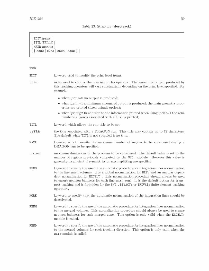
IGE–294 59

Table 23: Structure (desctrack)

[ EDIT iprint ][ TITL TITLE ][ MAXR maxreg ][ RENO | NORE | RENM | REND ]

with


iprint index used to control the printing of this operator. The amount of output produced bythis tracking operators will vary substantially depending on the print level specified. Forexample,

• when iprint=0 no output is produced;

• when iprint=1 a minimum amount of output is produced; the main geometry prop-erties are printed (fixed default option);

• when iprint≥2 In addition to the information printed when using iprint=1 the zonenumbering (zones associated with a flux) is printed;

TITL keyword which allows the run title to be set.

TITLE the title associated with a DRAGON run. This title may contain up to 72 characters.The default when TITL is not specified is no title.

MAXR keyword which permits the maximum number of regions to be considered during aDRAGON run to be specified.

maxreg maximum dimensions of the problem to be considered. The default value is set to thenumber of regions previously computed by the GEO: module. However this value isgenerally insufficient if symmetries or mesh-splitting are specified.

RENO keyword to specify the use of the automatic procedure for integration lines normalizationto the fine mesh volumes. It is a global normalization for NXT: and an angular depen-dent normalization for EXCELT:. This normalization procedure should always be usedto ensure neutron balances for each fine mesh zone. It is the default option for trans-port tracking and is forbidden for the SNT:, BIVACT: or TRIVAT: finite-element trackingoperators.

NORE keyword to specify that the automatic normalization of the integration lines should bedeactivated.

RENM keyword to specify the use of the automatic procedure for integration lines normalizationto the merged volumes. This normalization procedure should always be used to ensureneutron balances for each merged zone. This option is only valid when the EXCELT:

module is called.

REND keyword to specify the use of the automatic procedure for integration lines normalizationto the merged volumes for each tracking direction. This option is only valid when theNXT: module is called.

IGE–294 60

3.4.1 The SYBILT: tracking module

The geometries that can be treated by the module SYBILT: are

1. The homogeneous geometry HOMOGE.

2. The one-dimensional geometries SPHERE, TUBE and CAR1D.[49]

3. The two-dimensional geometries CAR2D and HEX including respectively CARCEL and HEXCEL sub-geometries as well as VIRTUAL sub-geometries.

4. Sij–type two-dimensional non-standard geometries.[8]

5. The double heterogeneity option.[47]

The calling specification for this module is:

Table 24: Structure (SYBILT:)

TRKNAM := SYBILT: [ TRKNAM ] GEONAM :: (desctrack) (descsybil)

where

TRKNAM character*12 name of the tracking data structure that will contain region volumeand surface area vectors in addition to region identification pointers and other trackinginformation. If TRKNAM also appears on the RHS, the previous tracking parameterswill be applied by default on the current geometry.

GEONAM character*12 name of the geometry data structure.

(desctrack) structure describing the general tracking data (see Section 3.4)

(descsybil) structure describing the transport tracking data specific to SYBILT:.

The SYBILT: specific tracking data in (descsybil) is defined as

Table 25: Structure (descsybil)

[ MAXJ maxcur ] [ MAXZ maxint ][ HALT ][ QUA1 iqua1 ] [ QUA2 iqua2 nsegment ] [ EQW | GAUS ][ ROTH | ROT+ | DP00 | DP01 ][ WIGN | ASKE | SANC ] [ LIGN ] [ RECT ][ [ QUAB iquab ] [ SAPO | HEBE ] ];

where

MAXJ keyword to specify the maximum number of interface currents surrounding the blocks inthe calculations.

IGE–294 61

maxcur the maximum number of interface currents surrounding the blocks. The default value ismaxcur=max(18,4×maxreg) for the SYBILT: module.

MAXZ keyword to specify the maximum amount of memory required to store the integrationlines. An insufficiently large value can lead to an execution failure (core dump).

maxint the maximum amount of memory required to store the integration lines. The defaultvalue is maxint=10000.

HALT keyword to specify that the program is to be stopped at the end of the geometry calcula-tions. This option permits the geometry inputs to be checked, the number of blocks andinterface currents to be calculated, and a conservative estimate of the memory requiredfor storing the tracks to be made for mixed geometries.

QUA1 keyword to specify the one-dimensional integration parameters.

iqua1 number of basis points for the angular integration of the blocks in a one-dimensionalgeometry. This parameter is not used for CAR1D geometries. If a Gauss-Legendre orGauss-Jacobi quadrature is used, the values of iqua1 allowed are: 1 to 20, 24, 28, 32 or64. The default value is iqua1=5.

QUA2 keyword to specify the two-dimensional integration parameters.

iqua2 number of basis points for the angular integration of the blocks in a two-dimensionalgeometry appearing during assembly calculations. If a Gauss-Legendre or Gauss-Jacobiformula is used the values allowed for iqua2 are: 1 to 20, 24, 28, 32 or 64. The defaultvalue is iqua2=3 and represents the number of angles in (0, π/4) for Cartesian geometriesand (0, π/6) for hexagonal geometries.

nsegment number of basis points for the spatial integration of the blocks in a two-dimensionalgeometry appearing during assembly calculations. The values of nsegment allowed are:1 to 10. The default value is nsegment=3.

EQW keyword to specify the use of equal-weight quadrature.

GAUS keyword to specify the use of the Gauss-Legendre or the Gauss-Jacobi quadrature. Thisis the default option.

ROTH keyword to specify that the isotropic (DP0) components of the inter-cell current is usedwith the incoming current being averaged over all the faces surrounding a cell. Theglobal collision matrix is calculated in a annular model. Only used when 2–d assemblyof cells are considered.

ROT+ keyword to specify that the isotropic (DP0) components of the inter-cell current is used.The global collision matrix is calculated in a annular model. Only used when 2–d as-sembly of cells are considered.

DP00 keyword to specify that the isotropic (DP0) components of the inter-cell current is used.The global collision matrix are computed explicitly. Only used when 2–d assembly ofcells are considered.

DP01 keyword to specify that the linearly anisotropic (DP1) components of the inter-cell cur-rent are used. This hypothesis implies 12 currents per cell in a cartesian geometry and18 currents per cell for an hexagonal geometry. Linearly anisotropic reflection is used.Only used when 2–d assembly of cells are considered.

WIGN keyword to specify the use of a Wigner cylinderization which preserves the volume ofthe external crown. This applies only in cases where the external surface is annularusing the ROTH or ROT+ options. Only used when 2–d assembly of cells are considered.Note that an assembly of rectangular cells having unequal volumes cannot use a Wignercylinderization.

IGE–294 62

ASKE keyword to specify the use of an Askew cylinderization which preserves both the externalsurface of the cells and the material balance of the external crown (by a modificationof its concentration). This applies only in cases where the external surface is annularusing the ROTH or ROT+ options. Only used when 2–d assembly of cells are considered.Note that an assembly of rectangular cells having unequal volumes can use an Askewcylinderization.

SANC keyword to specify the use of a Sanchez cylinderization. This model uses a Wigner cylin-derization for computing the collision Pij and leakage PiS probabilities. However, thereciprocity and conservation relations used to compute the incoming PSj and transmis-sion PSS probabilities are defined in the rectangular cell (with the exact surface).[50] Thisapplies where the external surface is annular using the ROTH or ROT+ options. Only usedwhen 2–d assembly of cells are considered. Note that an assembly of rectangular cellshaving unequal volumes can use a Sanchez cylinderization. This is the default option.

LIGN keyword to specify that all the integration lines are to be printed. This option shouldonly be used when absolutely necessary because it generates a rather large amount ofoutput. Only used when 2–d assembly of cells are considered.

RECT keyword to specify that square cells are to be treated as if they were rectangular cells,with the inherent loss in performance that this entails. This option is of purely academicinterest.

QUAB keyword to specify the number of basis point for the numerical integration of each micro-structure in cases involving double heterogeneity (Bihet).

iquab the number of basis point for the numerical integration of the collision probabilities inthe micro-volumes using the Gauss-Jacobi formula. The values permitted are: 1 to 20,24, 28, 32 or 64. The default value is iquab=5.

SAPO use the Sanchez-Pomraning double-heterogeneity model.[46]

HEBE use the Hebert double-heterogeneity model (default option).[47]

IGE–294 63

3.4.2 The EXCELT: tracking module


Table 26: Structure (EXCELT:)

TRKNAM [ TRKFIL ] := EXCELT: [ TRKNAM ] [ TRKFIL ]GEONAM :: (desctrack) (descexcel)

where


TRKFIL character*12 name of the sequential binary tracking file used to store the tracks lengths.If TRKFIL does not appear, the keyword XCLL is set automatically. If the user wants touse a tracking file, TRKFIL is required for the EXCELT: module, either on the LHS, onthe RHS or on both sides. In the case where TRKFIL appears on both LHS and RHS,the existing tracking file is modified by the module while if TRKFIL appears only onthe RHS, the existing tracking file is read but not modified.



(descexcel) structure describing the transport tracking data specific to EXCELT:.

The EXCELT: specific tracking data in (descexcel) is defined as

Table 27: Structure (descexcel)

[ ANIS nanis ][ ONEG | ALLG | XCLL ][ PISO | PSPC [ CUT pcut ] ][ [ QUAB iquab ] [ SAPO | HEBE ] ][ PRIX | PRIY | PRIZ denspr ][ LCMD | OPP1 | OGAU | GAUS | CACA | CACB [ nmu ] ][ TRAK [ CORN pcorn ] TISO nangl [ nangl z ] dens [ dens z ] [ SYMM isymm | NOSY ]

| TSPC [ MEDI ] nangl dens | HALT ];

where

ANIS keyword to specify the order of scattering anisotropy.

nanis order of anisotropy in transport calculation. A default value of 1 represents isotropic(or transport-corrected) scattering while a value of 2 correspond to linearly anisotropicscattering. When anisotropic scattering is considered, user should pay attention to thefollowing points:

IGE–294 64

• the usage of DIAG, SYME, SSYM keywords in the definition of the geometry is forbid-den. Indeed, in EXCELT:/NXT: tracking procedures, the geometry is “unfolded”according to these symmetries : this is incompatible with the integration of theanisotropic moments of the flux;

• the angular quadratures should be selected paying attention to the restrictionsmentioned in this manual in order to ensure the particle conservation.

ONEG keyword to specify that the tracking is read before computing each group-dependentcollision probability or algebraic collapsing matrix (default value if TRKFIL is set).The tracking file is read in each energy group if the method of characteristics (MOC)is used.

ALLG keyword to specify that the tracking is read once and the collision probability oralgebraic collapsing matrices are computed in many energy groups. The tracking fileis read once if the method of characteristics (MOC) is used.

XCLL keyword to specify that the tracking is computed on-demand (it is not stored on afile) and the collision probability matrices are computed in many energy groups. Thetracking file TRKFIL should not be provided (default value if TRKFIL is not set).

PISO keyword to specify that a collision probability calculation with isotropic reflectionboundary conditions is required. It is the default option if a TISO type integrationis chosen. To obtain accurate transmission probabilities for the isotropic case it isrecommended that the normalization options in the ASM: module be used.

PSPC keyword to specify that a collision probability calculation with specular reflectionboundary conditions required; this is the default option if a TSPC type integration ischosen. This calculation is only possible if the file was initially constructed using theTSPC option.

CUT keyword to specify the input of cutting parameters for the specular integration.

pcut real value representing the maximum error allowed on the exponential function usedfor specular collision probability calculations. Tracks will be cut at a length such thatthe error in the probabilities resulting from this reduced track will be of the order ofpcut. By default, there is no cutting of the tracks and pcut=0.0. If this option is usedin an entirely reflected case, it is preferable to use the NORM command in the ASM:

module.

QUAB keyword to specify the number of basis point for the numerical integration of eachmicro-structure in cases involving double heterogeneity (Bihet).

iquab the number of basis point for the numerical integration of the collision probabilitiesin the micro-volumes using the Gauss-Jacobi formula. The values permitted are: 1 to20, 24, 28, 32 or 64. The default value is iquab=5.



PRIX keyword to specify that a prismatic tracking is considered for a 3D geometry invariantalong the x− axis. In this case, the 3D geometry is projected in the y− z plane and a2D tracking on the projected geometry is performed. This capability is limited to thenon-cyclic method of characteristics solver for the time being and a subsequent call toMCCGT: is mandatory.

PRIY keyword to specify that a prismatic tracking is considered for a 3D geometry invariantalong the y− axis. In this case, the 3D geometry is projected in the z− x plane and a2D tracking on the projected geometry is performed. This capability is limited to the

IGE–294 65

method of characteristics solver for the time being and a subsequent call to MCCGT: ismandatory.

PRIZ keyword to specify that a prismatic tracking is considered for a 3D geometry invariantalong the z− axis. In this case, the 3D geometry is projected in the x− y plane and a2D tracking on the projected geometry is performed. This capability is limited to themethod of characteristics solver for the time being and a subsequent call to MCCGT: ismandatory.

denspr real value representing the linear track density (in cm−1) to be used for the inlinecontruction of 3D tracks from 2D tracking when a prismatic tracking is considered.

LCMD keyword to specify that optimized (McDaniel–type) polar integration angles are to beselected for the polar quadrature when a prismatic tracking is considered.[42] This isthe default option. The conservation is ensured only for isotropic scattering.

OPP1 keyword to specify that P1 constrained optimized (McDaniel–type) polar integra-tion angles are to be selected for the polar quadrature when a prismatic tracking isconsidered.[43] The conservation is ensured only for isotropic and linearly anisotropicscattering.

OGAU keyword to specify that Optimized Gauss polar integration angles are to be selectedfor the method of characteristics.[42, 43] The conservation is ensured up to Pnmu−1scattering.

GAUS keyword to specify that Gauss-Legendre polar integration angles are to be selectedfor the polar quadrature when a prismatic tracking is considered. The conservation isensured up to Pnmu−1 scattering.

CACA keyword to specify that CACTUS type equal weight polar integration angles are tobe selected for the polar quadrature when a prismatic tracking is considered.[44] Theconservation is ensured only for isotropic scattering.

CACB keyword to specify that CACTUS type uniformly distributed integration polar anglesare to be selected for the polar quadrature when a prismatic tracking is considered.[44]

The conservation is ensured only for isotropic scattering.

nmu user-defined number of polar angles. By default, a value consistent with nangl iscomputed by the code. For LCMD, OPP1, OGAU quadratures, nmu is limited to 2, 3 or 4.

TRAK keyword to specify the tracking parameters to be used.

TISO keyword to specify that isotropic tracking parameters will be supplied. This is thedefault tracking option for cluster geometries.

TSPC keyword to specify that specular tracking parameters will be supplied.

MEDI keyword to specify that instead of selecting the angles located at the end of eachangular interval, the angles located in the middle of these intervals are selected. Thisis particularly useful if one wants to avoid tracking angles that are parallel to the X−or Y−axis as its is the case when the external region of a CARCEL geometry is voided.

nangl angular quadrature parameter. For applications involving 3–D cells, the choices arenangl=2, 4, 8, 10, 12, 14 or 16; these angular quadratures EQn present a rotationalsymmetry about the three cartesian axes. For 2–D isotropic applications, any valueof nangl ≥ 2 may be used; equidistant angles will be selected. For 2–D specularapplications the input value must be of the form p + 1 where p is a prime number(for example p=7, 11, etc.); the choice of nangl = 8, 12, 14, 18, 20, 24, or 30 areallowed. For cluster type geometries the default value is nangl=10 for isotropic casesand nangl=12 for specular cases.

IGE–294 66

nangl z angular quadrature parameter in the axial Z direction. Used only with HEXZ andHEXCELZ geometries.

dens real value representing the density of the integration lines (in cm−1 for 2–D cases andcm−2 for 3–D cases). This choice of density along the plan perpendicular to each angledepends on the geometry of the cell to be analyzed. If there are zones of very smallvolume, a high line density is essential. This value will be readjusted by EXCELT:. Inthe case of the analysis of a cluster type geometry the default value of this parameteris 5/rm where rm is the minimum radius of the pins or the minimum thickness of anannular ring in the geometry. If the selected value of dens is too small, some volumesor surfaces may not be tracked.

dens z real value representing the density of the integration lines in the axial Z direction.Used only with HEXZ and HEXCELZ geometries.

CORN keyword to specify that the input of the parameters used to treat the corners for theisotropic integration.

pcorn maximum distance (cm) between a line and the intersection of n ≥ 2 external surfaceswhere track redistribution will take place. Track redistribution will take place if a linecomes close to the intersection of n ≥ 2 external surfaces. In this case the line will bereplicated n times, each of these lines being associated with a different external surface,while its weight is reduced by a factor of 1/n. This allows for a better distributionof tracks which are relatively close to n external surfaces. By default, there is notreatment of the corners and pcorn=0.0.

SYMM keyword to specify that the geometry has a rotation symmetry.

isymm integer value describing the rotation symmetry of the geometry. The fixed default ofthis parameter is 1.

NOSY EXCELT: automatically try to take into account geometric symmetries in order toreduce the number of tracks and the CPU time. The NOSY keyword desactivates thisautomatic capability.

HALT keyword to specify that the program is to be stopped after the analysis of the geometry,without the explicit tracking being performed.

IGE–294 67

3.4.3 The NXT: tracking module


Table 28: Structure (NXT:)

[ TRKFIL ] TRKNAM := NXT: [ TRKNAM ] [ GEONAM ] :: (desctrack) (descnxt)

where


TRKFIL character*12 name of the sequential binary tracking file used to store the tracks lengths.If TRKFIL does not appear, the keyword XCLL is set automatically. If the user wants touse a tracking file, TRKFIL is required.



(descnxt) structure describing the transport tracking data specific to NXT:.

The NXT: specific tracking data in (descnxt) is defined as

Table 29: Structure (descnxt)

[ ANIS nanis ][ ONEG | ALLG | XCLL ][ [ QUAB iquab ] [ SAPO | HEBE ] ][ PISO | PSPC [ CUT pcut ] ][ SYMM isymm | NOSY ][ GAUS | CACA | CACB | LCMD | OPP1 | OGAU [ nmu ] ] TISO [ EQW | GAUS | PNTN | SMS | LSN | QRN ] nangl dens [ CORN pcorn ]| TSPC [ MEDI ] nangl dens

[ NOTR | MC ][ NBSLIN nbslin ][ LONG ][ PRIZ denspr ];

where

ANIS keyword to specify the order of scattering anisotropy.

nanis order of anisotropy in transport calculation. A default value of 1 represents isotropic(or transport-corrected) scattering while a value of 2 correspond to linearly anisotropic

IGE–294 68

scattering. When anisotropic scattering is considered, user should pay attention to thefollowing points:

• the usage of DIAG, SYME, SSYM keywords in the definition of the geometry is forbid-den. Indeed, in EXCELT:/NXT: tracking procedures, the geometry is “unfolded”according to these symmetries : this is incompatible with the integration of theanisotropic moments of the flux;

• an angular dependent normalization of the track lengths should be requested inthe tracking procedure (REND keyword) in order to ensure the particle conserva-tion;

• the angular quadratures should be selected paying attention to the restrictionsmentioned in this manual in order to ensure the particle conservation.

ONEG keyword to specify that the tracking is read before computing each group-dependentcollision probability or algebraic collapsing matrix (default value if TRKFIL is set).The tracking file is read in each energy group if the method of characteristics (MOC)is used.

ALLG keyword to specify that the tracking is read once and the collision probability oralgebraic collapsing matrices are computed in many energy groups. The tracking fileis read once if the method of characteristics (MOC) is used.

XCLL keyword to specify that the tracking is computed on-demand (it is not stored on afile) and the collision probability matrices are computed in many energy groups. Thetracking file TRKFIL should not be provided (default value if TRKFIL is not set).

QUAB keyword to specify the number of basis point for the numerical integration of eachmicro-structure in cases involving double heterogeneity (Bihet).

iquab the number of basis point for the numerical integration of the collision probabilitiesin the micro-volumes using the Gauss-Jacobi formula. The values permitted are: 1 to20, 24, 28, 32 or 64. The default value is iquab = 5.



PISO keyword to specify that a collision probability calculation with isotropic reflectionboundary conditions is required. It is the default option if a TISO type integrationis chosen. To obtain accurate transmission probabilities for the isotropic case it isrecommended that the normalization options in the ASM: module be used.

PSPC keyword to specify that a collision probability calculation with mirror like reflection orperiodic boundary conditions is required; this is the default option if a TSPC type inte-gration is chosen. This calculation is only possible if the file was initially constructedusing the TSPC option.

CUT keyword to specify the input of cutting parameters for the specular collision probabilityof characteristic integration.

pcut real value representing the maximum error allowed on the exponential function usedfor specular collision probability calculations. Tracks will be cut at a length such thatthe error in the probabilities resulting from this reduced track will be of the order ofpcut. By default, the tracks are extended to infinity and pcut = 0.0. If this option isused in an entirely reflected case, it is recommended to use the NORM command in theASM: module.

IGE–294 69

SYMM keyword to specify the level to which the tracking will respect the symmetry of thegeometry.

isymm level to which the tracking will respect the symmetry of the geometry. For 2-D and3-D Cartesian geometries it must takes the form isymm=2Sx + 4Sy + 16Sz where

• Sx = 1 if the X symmetry is to be considered and Sx = 0 otherwise.

• Sy = 1 if the Y symmetry is to be considered and Sy = 0 otherwise.

• Sz = 1 if the Z symmetry is to be considered and Sz = 0 otherwise.

NOSY keyword to specify the full tracking will take place irrespective of the symmetry of thegeometry. This is equivalent to specifying isymm=0.

GAUS keyword to specify that Gauss-Legendre polar integration angles are to be selectedfor the polar quadrature when a prismatic tracking is considered. The conservation isensured up to Pnmu−1 scattering.

CACA keyword to specify that CACTUS type equal weight polar integration angles are tobe selected for the polar quadrature when a prismatic tracking is considered.[44] Theconservation is ensured only for isotropic scattering.

CACB keyword to specify that CACTUS type uniformly distributed integration polar anglesare to be selected for the polar quadrature when a prismatic tracking is considered.[44]

The conservation is ensured only for isotropic scattering.

LCMD keyword to specify that optimized (McDaniel–type) polar integration angles are to beselected for the polar quadrature when a prismatic tracking is considered.[42] This isthe default option. The conservation is ensured only for isotropic scattering.

OPP1 keyword to specify that P1 constrained optimized (McDaniel–type) polar integra-tion angles are to be selected for the polar quadrature when a prismatic tracking isconsidered.[43] The conservation is ensured only for isotropic and linearly anisotropicscattering.


nmu user-defined number of polar angles. By default, a value consistent with nangl iscomputed by the code. For LCMD, OPP1, OGAU quadratures, nmu is limited to 2, 3 or 4.

TISO keyword to specify that isotropic tracking parameters will be supplied. This is thedefault tracking option for cluster geometries.

TSPC keyword to specify that specular tracking parameters will be supplied.

EQW keyword to specify the use of equal weight quadrature.[37] The conservation is ensuredup to Pnangl/2 scattering.

GAUS (after TISO keyword) keyword to specify the use of the Gauss-Legendre quadrature.This option is valid only if an hexagonal geometry is considered.

PNTN keyword to specify that Legendre-Techbychev quadrature quadrature will be selected.[38]

The conservation is ensured only for isotropic and linearly anisotropic scattering.

SMS keyword to specify that Legendre-trapezoidal quadrature quadrature will be selected.[39]

The conservation is ensured up to Pnangl−1 scattering.

LSN keyword to specify the use of the µ1–optimized level-symmetric quadrature. Theconservation is ensured up to Pnangl/2 scattering.

IGE–294 70

QRN keyword to specify the use of the quadrupole range (QR) quadrature.[29]

MEDI keyword to specify the use of a median angle quadrature. Instead of selecting theangles located at the end of each angular interval, the angles located in the middle ofthese intervals are selected. This is particularly useful if one wants to avoid trackingangles that are parallel to the X− or Y−axis as its is the case when the external regionof a CARCEL geometry is voided.

nangl angular quadrature parameter. For a 3-D EQW option, the choices are nangl = 2, 4,8, 10, 12, 14 or 16. For a 3-D PNTN or SMS option, nangl is an even number smallerthan 46.[36] For 2-D isotropic applications, any value of nangl may be used, equidistantangles will be selected. For 2-D specular applications the input value must be of theform p+1 where p is a prime number, as proposed in Ref. 25. In this case, the choiceof nangl = 8, 12, 14, 18, 20, 24, or 30 are allowed.

dens real value representing the density of the integration lines (in cm−1 for 2-D Cartesiancases and 3-D hexagonal cases and cm−2 for 3-D cases Cartesian cases). This choice ofdensity along the plan perpendicular to each angle depends on the geometry of the cellto be analyzed. If there are zones of very small volume, a high line density is essential.This value will be readjusted by NXT:.

CORN keyword to specify that the input of the parameters used to treat the corners for theisotropic integration.

pcorn maximum distance (cm) between a line and the intersection of n ≥ 2 external surfaceswhere track redistributing will take place. Track redistribution will take place if a linecomes close to the intersection of n ≥ 2 external surfaces. In this case the line will bereplicated n times, each of these lines being associated with a different external surface,while its weight is reduced by a factor of 1/n. This allows for a better distributionof tracks which are relatively close to n external surfaces. By default, there is notreatment of the corners and pcorn = 0.0.

NOTR keyword to specify that the geometry will not be tracked. This is useful for 2-Dgeometries to generate a tracking data structure that can be used by the PSP: module(see Section 3.26). One can then verify visually if the geometry is adequate before thetracking process as such is undertaken.

MC keyword to specify that the geometry will not be tracked and that object TRKNAMwill be used with the Monte-Carlo method. This option is similar to NOTR with addi-tional information being added into TRKNAM .

NBSLIN keyword to set the maximum number of segments in a single tracking line.

nbsl integer value representing the maximum number of segments in a single tracking line.The default value is nbsl = 100000.

LONG keyword to specify that a “long” tracking file will be generated. This option is requiredif the tracking file is to be used by the TLM: module (see Section 3.15).

PRIZ keyword to specify that a prismatic tracking is considered for a 3D geometry invariantalong the z− axis. In this case, the 3D geometry is projected in the x− y plane and a2D tracking on the projected geometry is performed. This capability is limited to thenon-cyclic method of characteristics solver for the time being and a subsequent call toMCCGT: is mandatory.

denspr real value representing the linear track density (in cm−1) to be used for the inlinecontruction of 3D tracks from 2D tracking when a prismatic tracking is considered.

IGE–294 71

3.4.4 The MCCGT: tracking module

This module must follow a call to module EXCELT: or NXT:. Its calling specification is:

Table 30: Structure (MCCGT:)

TRKNAM := MCCGT: TRKNAM TRKFIL [ GEONAM ] :: (descmccg)

where

TRKNAM character*12 name of the tracking data structure that will contain region volumeand surface area vectors in addition to region identification pointers and other track-ing information. It is provided by EXCELT: or NXT: operator and modified by MCCGT:

operator.

TRKFIL character*12 name of the sequential binary tracking file used to store the tracks lengths.This file is provided by EXCELT: or NXT: operator and used without modification byMCCGT: operator.

GEONAM character*12 name of the optional geometry data structure. This structure is onlyrequired to recover double-heterogeneity data.

(descmccg) structure describing the transport tracking data specific to MCCGT:.

The MCCGT: specific tracking data in (descmccg) is defined as

Table 31: Structure (descmccg)

[ EDIT iprint ][ LCMD | OPP1 | OGAU | GAUS | CACA | CACB [ nmu ] ] DIFC NONE | DIAG | FULL | ILU0 [ TMT ] [ LEXA ]|[ [ AAC iaca NONE | DIAG | FULL | ILU0 [ TMT ] ] [ SCR iscr ] [ LEXA ] ][ KRYL ikryl ][ MCU imcu ][ HDD xhdd ][ LEXF ][ STIS istis ]

[ MAXI nmaxi ][ EPSI xepsi ][ ADJ ]

;

where


iprint index used to control the printing in this operator.

IGE–294 72

LCMD keyword to specify that optimized (McDaniel–type) polar integration angles are to beselected for the method of characteristics.[42] This is the default option. The conser-vation is ensured only for isotropic scattering.

OPP1 keyword to specify that P1 constrained optimized (McDaniel–type) polar integrationangles are to be selected for the method of characteristics.[43] The conservation isensured only for isotropic and linearly anisotropic scattering.


GAUS keyword to specify that Gauss-Legendre polar integration angles are to be selected forthe method of characteristics. The conservation is ensured up to Pnmu−1 scattering.

CACA keyword to specify that CACTUS type equal weight polar integration angles are tobe selected for the method of characteristics.[44] The conservation is ensured only forisotropic scattering.

CACB keyword to specify that CACTUS type uniformly distributed integration polar anglesare to be selected for the method of characteristics.[44] The conservation is ensuredonly for isotropic scattering.

nmu user-defined number of polar angles for the integration of the tracks with the methodof characteristics for 2D geometries. By default, a value consistent with nangl iscomputed by the code. For LCMD, OPP1, OGAU quadratures, nmu is limited to 2, 3 or 4.

DIFC keyword used to specify that only an ACA-simplified transport flux calculation is tobe performed (not by default). In this case, the maximum number of ACA iterationsis set to nmaxi.

LEXA keyword used to force the usage of exact exponentials in the preconditioner calculation(not by default).

MAXI keyword to specify the maximum number of scattering iterations performed in eachenergy group. This keyword is also used to set the number of Bi-CGSTAB iterationsto solve the ACA-simplified system if DIFC is present.

nmaxi the maximum number of iterations. The default value is nmaxi=20.

EPSI keyword to specify the convergence criterion on inner iterations (or ACA-simplifiedflux calculation if DIFC is present).

xepsi convergence criterion. The default value is xepsi=1.0×10−4.

AAC keyword to set the ACA preconditioning of inner/multigroup iterations in case wherea transport solution is selected.[21, 27]

iaca 0/> 0: ACA preconditioning of inner or multigroup iterations off/on. The defaultvalue is iaca=1. If MAXI is set to 1, ACA is used as a rebalancing technique formultigroup-inner mixed iterations and iaca is the maximum number of iterations al-lowed to solve the ACA system (e.g. 100).

NONE no preconditioning for the iterative resolution by Bi-CGSTAB of the ACA system.

DIAG diagonal preconditioning for the iterative resolution by Bi-CGSTAB of the ACA sys-tem.

FULL full-matrix preconditioning for the iterative resolution by Bi-CGSTAB of the ACAsystem.

IGE–294 73

ILU0 ILU0 preconditioning for the iterative resolution by Bi-CGSTAB of the ACA system(This is the default option).

TMT two-step collapsing version of ACA which uses a tracking merging technique whilebuilding the ACA matrices.

SCR keyword to set the SCR preconditioning of inner/multigroup iterations.[28]

iscr 0/> 0: SCR preconditioning of inner or multigroup iterations off/on. The default valueis iscr=0. If MAXI is set to 1, SCR is used as a rebalancing technique for multigroup-inner mixed iterations and iscr is the maximum number of iterations allowed to solvethe SCR system. When anisotropic scattering is considered, SCR provides an accel-eration of anisotropic flux moments. If both ACA and SCR are selected (iscr> 0 andiaca> 0), a two-step acceleration scheme (equivalent to ACA when isotropic scatteringis considered) involving both methods is used.

KRYL keyword to enable the Krylov acceleration of scattering iterations performed in eachenergy group.[28]

ikryl 0: GMRES/Bi-CGSTAB acceleration not used; > 0: dimension of the Krylov subspacein GMRES; < 0: Bi-CGSTAB is used. The default value is ikryl=10.

MCU keyword used to specify the maximum dimension of the connection matrix for memoryallocation.

imcu The default value is eight (resp. twelve) times the number of volumes and externalsurfaces for 2D (resp. 3D) geometries.

HDD keyword to select the integration scheme along the tracking lines.

xhdd selection criterion:

xhdd =

0.0 step characteristics scheme> 0.0 diamond differencing scheme.

The default value is xhdd=0.0 so that the step characteristics method is used.

LEXF keyword used to force the usage of exact exponentials in the flux calculation (not bydefault).

STIS keyword to select the tracking integration strategy.

istis 0: a direct approach with asymptotical treatment is used; 1: a “source term isola-tion” approach with asymptotical treatment is used (this technique tends to reducethe computational cost and increase the numerical stability but requires the calcula-tion of angular mode-to-mode self-collision probabilities); −1: an ”MOCC/MCI”-likeapproach is used (it tends to reduce further more the computational cost as it doesn’tfeature any asymptotical treatment for vanishing optical thicknesses). Note that whena zero total cross section is found with istis=-1, it is reset to 1. The default value isistis=1 for PL≤3 anisotropy and 0 otherwise.

ADJ keyword to select an adjoint solution of ACA and characteristics systems. A directsolution is set by default.

IGE–294 74

3.4.5 The SNT: tracking module

The SNT:module can process one-dimensional, two-dimensional regular geometries and three-dimensionalCartesian geometries of type CAR1D, TUBE, SPHERE, CAR2D, TUBEZ and CAR3D.


Table 32: Structure (SNT:)

TRKNAM := SNT: [ TRKNAM ] GEONAM :: (desctrack) (descsn)

where




(descsn) structure describing the transport tracking data specific to SNT:.

The SNT: specific tracking data in (descsn) is defined as

Table 33: Structure (descsn)

[ DIAM m ]SN n [ SCAT iscat ] [ DSA | NDSA ] [ LIVO icl1 icl2 | NLIVO ][ GMRES nstart ] [ NSDSA nsdsa ] [ MAXI maxi ] [ EPSI epsi ] [ QUAD iquad ][ [ QUAB iquab ] [ SAPO | HEBE ] ];

where


DIAM keyword to fix the spatial approximation order.

m spatial order. m = 1 is used for the classical diamond scheme (default value). m = 2 or= 3 is currently available in 1D slab, 2D Cartesian and 3D Cartesian geometries.

SN keyword to fix the angular approximation order of the flux.

n order of the SN approximation (even number).

SCAT keyword to limit the anisotropy of scattering sources.

iscat number of terms in the scattering sources. iscat = 1 is used for isotropic scattering in thelaboratory system. iscat = 2 is used for linearly anisotropic scattering in the laboratorysystem. The default value is set to n.

IGE–294 75

LIVO keyword to enable Livolant acceleration method (default value).

icl1 , icl2 Numbers of respectively free and accerated iterations in the Livolant method.

NLIVO keyword to disable Livolant acceleration method.

DSA keyword to enable diffusion synthetic acceleration using BIVAC or TRIVAC (defaultvalue).

NDSA keyword to disable diffusion synthetic acceleration.

GMRES keyword to set the GMRES(m) acceleration of the scattering iterations. The defaultvalue, equivalent to nstart=0, corresponds to a one-parameter Livolant acceleration.[28]

nstart restarts the GMRES method every nstart iterations.

NSDSA keyword to set the number if inner flux iterations without DSA in 3D cases if m ≥ 2. IfDSA is enabled too soon, instabilities and convergence failure can occur in these cases.

nsdsa number if inner flux iterations without DSA. The default value is nsdsa = 10.

MAXI Keyword to set the maximum number of inner iterations (or GMRES iterations if ac-tived).

maxi Maximum number of inner iterations. Default value: 100.

EPSI Set the convergence criterion on inner iterations (or GMRES iterations if actived).

epsi Convergence criterion on inner iterations. The default value is 1× 10−5.

QUAD keyword to set the type of angular quadrature.

iquad type of quadrature: = 1: Lathrop-Carlson level-symmetric quadrature; = 2: µ1–optimi-zed level-symmetric quadrature (default option in 2D and in 3D); = 3 Snow-code level-symmetric quadrature (obsolete); = 4: Legendre-Chebyshev quadrature (variable num-ber of base points per axial level); = 5: symmetric Legendre-Chebyshev quadrature;= 6: quadruple range (QR) quadrature;[29] = 10: product of Gauss-Legendre and Gauss-Chebyshev quadrature (equal number of base points per axial level).

QUAB keyword to specify the number of basis point for the numerical integration of each micro-structure in cases involving double heterogeneity (Bihet).

iquab the number of basis point for the numerical integration of the collision probabilities inthe micro-volumes using the Gauss-Jacobi formula. The values permitted are: 1 to 20,24, 28, 32 or 64. The default value is iquab=5.



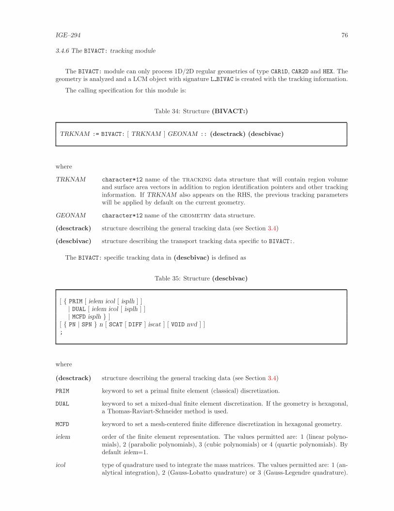
IGE–294 76

3.4.6 The BIVACT: tracking module

The BIVACT: module can only process 1D/2D regular geometries of type CAR1D, CAR2D and HEX. Thegeometry is analyzed and a LCM object with signature L BIVAC is created with the tracking information.


Table 34: Structure (BIVACT:)

TRKNAM := BIVACT: [ TRKNAM ] GEONAM :: (desctrack) (descbivac)

where




(descbivac) structure describing the transport tracking data specific to BIVACT:.

The BIVACT: specific tracking data in (descbivac) is defined as

Table 35: Structure (descbivac)

[ PRIM [ ielem icol [ isplh ] ]| DUAL [ ielem icol [ isplh ] ]| MCFD isplh ]

[ PN | SPN n [ SCAT [ DIFF ] iscat ] [ VOID nvd ] ];

where


PRIM keyword to set a primal finite element (classical) discretization.

DUAL keyword to set a mixed-dual finite element discretization. If the geometry is hexagonal,a Thomas-Raviart-Schneider method is used.

MCFD keyword to set a mesh-centered finite difference discretization in hexagonal geometry.

ielem order of the finite element representation. The values permitted are: 1 (linear polyno-mials), 2 (parabolic polynomials), 3 (cubic polynomials) or 4 (quartic polynomials). Bydefault ielem=1.

icol type of quadrature used to integrate the mass matrices. The values permitted are: 1 (an-alytical integration), 2 (Gauss-Lobatto quadrature) or 3 (Gauss-Legendre quadrature).

IGE–294 77

By default icol=2. The analytical integration corresponds to classical finite elements;the Gauss-Lobatto quadrature corresponds to a variational or nodal type collocation andthe Gauss-Legendre quadrature corresponds to superconvergent finite elements.

isplh type of hexagonal mesh-splitting. This data is given only if the geometry is 2-D hexago-nal. The values permitted with the finite difference discretizations are: 1 (full hexagons),2 for splitting each hexagon into 6 triangles, 3 for splitting each hexagon into 24 trian-gles, 5 for splitting each hexagon into 96 triangles, 9 for splitting each hexagon into 384triangles and 17 for splitting each hexagon into 1536 triangles. The values permittedwith the Thomas-Raviart-Schneider method are: 1 (full hexagons), > 1 for performinga mesh-splitting in 3×isplh2 losanges per hexagon.

PN keyword to set a spherical harmonics (Pn) expansion of the flux.[53] This option is cur-rently limited to 1D and 2D Cartesian geometries.

SPN keyword to set a simplified spherical harmonics (SPn) expansion of the flux.[53, 54] Thisoption is currently available with 1D and 2D Cartesian geometries and with 2D hexagonalgeometries.

n order of the Pn or SPn expansion (odd number). Set to zero for diffusion theory (defaultvalue).


DIFF keyword to force using 1/3Dg as Σg1 cross sections. A P1 or SP1 method will therefore

behave as diffusion theory.

iscat number of terms in the scattering sources. iscat = 1 is used for isotropic scattering in thelaboratory system. iscat = 2 is used for linearly anisotropic scattering in the laboratorysystem. The default value is set to n+ 1 in Pn or SPn case.

VOID key word to set the number of base points in the Gauss-Legendre quadrature used tointegrate void boundary conditions if icol = 3 and n 6= 0.

nvd type of quadrature. The values permitted are: 0 (use a (n+2)–point quadrature consis-tent with Pn theory), 1 (use a (n+1)–point quadrature consistent with Sn+1 theory), 2(use an analytical integration of the void boundary conditions). By default nvd=0.

Various finite element approximations can be obtained by combining different values of ielem and icol:

• PRIM 1 1 : Linear finite elements;

• PRIM 1 2 : Mesh corner finite differences;

• PRIM 1 3 : Linear superconvergent finite elements;

• PRIM 2 1 : Quadratic finite elements;

• PRIM 2 2 : Quadratic variational collocation method;

• PRIM 2 3 : Quadratic superconvergent finite elements;

• PRIM 3 1 : Cubic finite elements;

• PRIM 3 2 : Cubic variational collocation method;

• PRIM 3 3 : Cubic superconvergent finite elements;

• PRIM 4 2 : Quartic variational collocation method;

• DUAL 1 1 : Mixed-dual linear finite elements;

• DUAL 1 2 : Mesh centered finite differences;

IGE–294 78

• DUAL 1 3 : Mixed-dual linear superconvergent finite elements

(numerically equivalent to PRIM 1 3);

• DUAL 2 1 : Mixed-dual quadratic finite elements;

• DUAL 2 2 : Quadratic nodal collocation method;

• DUAL 2 3 : Mixed-dual quadratic superconvergent finite elements


• DUAL 3 1 : Mixed-dual cubic finite elements;

• DUAL 3 2 : Cubic nodal collocation method;

• DUAL 3 3 : Mixed-dual cubic superconvergent finite elements


• DUAL 4 2 : Quartic nodal collocation method;

IGE–294 79

3.4.7 The TRIVAT: tracking module

The TRIVAT:module is used to perform a TRIVAC-type “tracking” on a 1D/2D/3D regular Cartesianor hexagonal geometry.[51, 52] The geometry is analyzed and a LCM object with signature L TRIVAC iscreated with the following information:

• Diagonal and hexagonal symmetries are unfolded and the mesh-splitting operations are performed.Volumes, material mixture and averaged flux recovery indices are computed on the resulting geom-etry.

• A finite element discretization is performed and the corresponding numbering is saved.

• The unit finite element matrices (mass, stiffness, etc.) are recovered.

• Indices related to an ADI preconditioning with or without supervectorization are saved.


Table 36: Structure (TRIVAT:)

TRKNAM := TRIVAT: [ TRKNAM ] GEONAM :: (desctrack) (descTRIVAC)

where




(descTRIVAC) structure describing the transport tracking data specific to TRIVAT:.

The TRIVAT: specific tracking data in (descTRIVAC) is defined as

Table 37: Structure (descTRIVAC)

[ PRIM [ ielem [ isplh ] ] | DUAL [ ielem icol [ isplh ] ] | MCFD [ ielem [ isplh ] ] | LUMP [ ielem ] ][ SPN n [ SCAT [ DIFF ] iscat ] [ VOID nvd ] ][ ADI nadi ][ VECT [ iseg ] [ PRTV impv ] ];

where


PRIM key word to set a discretization based on the variational collocation method.

IGE–294 80

DUAL key word to set a mixed-dual finite element discretization. If the geometry is hexagonal, aThomas-Raviart-Schneider method is used.

MCFD key word to set a discretization based on the nodal collocation method. The mesh centeredfinite difference approximation is the default option and is generally set using MCFD 1. TheMCFD approximations are numerically equivalent to the DUAL approximations with icol=2;however, the MCFD approximations are less expensive.

LUMP key word to set a discretization based on the nodal collocation method with serendipityapproximation. The serendipity approximation is different from the MCFD option in caseswith ielem≥2. This option is not available for hexagonal geometries.

ielem order of the finite element representation. The values permitted are: 1 (linear polynomials),2 (parabolic polynomials), 3 (cubic polynomials) or 4 (quartic polynomials). By defaultielem=1.

icol type of quadrature used to integrate the mass matrices. The values permitted are: 1(analytical integration), 2 (Gauss-Lobatto quadrature) or 3 (Gauss-Legendre quadrature).By default icol=2. The analytical integration corresponds to classical finite elements; theGauss-Lobatto quadrature corresponds to a variational or nodal type collocation and theGauss-Legendre quadrature corresponds to superconvergent finite elements.

isplh type of hexagonal mesh-splitting. This data is given only if the geometry is 2D or 3Dhexagonal. The values permitted with the MCFD option are: 1 (full hexagons), 2 for splittingeach hexagon into 6 triangles, 3 for splitting each hexagon into 24 triangles, etc. The valuespermitted with the PRIM option are: 1 (full hexagons) and 2 for splitting each hexagon into6 triangles. The values permitted with the Thomas-Raviart-Schneider method are: 1 (fullhexagons), > 1 for performing a mesh-splitting in 3×isplh2 losanges per hexagon.

SPN keyword to set a simplified spherical harmonics (SPn) expansion of the flux.[53, 54] Thisoption is available with 1D, 2D and 3D Cartesian geometries and with 2D and 3D hexagonalgeometries.

n order of the Pn or SPn expansion (odd number). Set to zero for diffusion theory (defaultvalue).


DIFF keyword to force using 1/3Dg as Σg1 cross sections. A P1 or SP1 method will therefore

behave as diffusion theory.

iscat number of terms in the scattering sources. iscat = 1 is used for isotropic scattering in thelaboratory system. iscat = 2 is used for linearly anisotropic scattering in the laboratorysystem. The default value is set to n+ 1 in Pn or SPn case.

VOID key word to set the number of base points in the Gauss-Legendre quadrature used tointegrate void boundary conditions if icol = 3 and n 6= 0.

nvd type of quadrature. The values permitted are: 0 (use a (n+2)–point quadrature consistentwith Pn theory), 1 (use a (n+1)–point quadrature consistent with Sn+1 theory), 2 (use ananalytical integration of the void boundary conditions). By default nvd=0.

ADI keyword to set the number of ADI iterations at the inner iterative level.

nadi number of ADI iterations (default: nadi = 2).

VECT key word to set an ADI preconditionning with supervectorization. By default, TRIVACuses an ADI preconditionning without supervectorization.

iseg width of a vectorial register. iseg is generally a multiple of 64. By default, iseg=64.

PRTV key word used to set impv .

IGE–294 81

impv index used to control the printing in supervectorization subroutines. =0 for no print; =1for minimum printing (default value); Larger values produce increasing amounts of output.

Various finite element approximations can be obtained by combining different values of ielem andisplh.

IGE–294 82

3.5 The SHI: module

The self-shielding module in DRAGON, called SHIBA[55], allows the energy-dependent dilution pa-rameter (microscopic dilution cross section) associated with each resonant isotope, identified as such bythe inrs parameter defined in Section 3.2, to be recalculated. The general format of the data for thismodule is:

Table 38: Structure (SHI:)

MICLIB := SHI: MICLIB | OLDLIB TRKNAM [ TRKFIL ] :: (descshi)

where

MICLIB character*12 name of the microlib that will contain the microscopic and macro-scopic cross sections updated by the self-shielding module. If MICLIB appears onboth LHS and RHS, it is updated; otherwise, the internal library OLDLIB is copiedinto MICLIB and MICLIB is updated.

OLDLIB character*12 name of a read-only microlib that is copied into MICLIB.

TRKNAM character*12 name of the required tracking data structure.

TRKFIL character*12 name of the sequential binary tracking file used to store the trackslengths. This file is given if and only if it was required in the previous tracking modulecall (see Section 3.4).

(descshi) structure describing the self-shielding options.

Each time the SHI: module is called, a sub-directory is updated in the microlib data structure tohold the last values defined in the (descshi) structure. The next time this module is called, these valueswill be used as floating defaults.

3.5.1 Data input for module SHI:

Table 39: Structure (descshi)

[ EDIT iprint ][ GRMIN lgrmin ] [ GRMAX lgrmax ][ MXIT imxit ] [ EPS valeps ][ LJ | NOLJ ] [ GC | NOGC ] [ NOTR ][ LEVEL ilev ][ PIJ | ARM ];

where


IGE–294 83

iprint index used to control the printing of this module. The amount of output produced bythis tracking module will vary substantially depending on the print level specified.

GRMIN keyword to specify the minimum group number considered during the self-shieldingprocess.

lgrmin first group number considered during the self-shielding process. By default, lgrmin isset to the first group number containing self-shielding data in the library.

GRMAX keyword to specify the maximum group number considered during the self-shieldingprocess.

lgrmax last group number considered during the self-shielding process. By default, lgrmax isset is set to the last group number containing self-shielding data in the library.

MXIT keyword to specify the maximum number of iterations during the self-shielding process.

imxit the maximum number of iterations. The default is imxit=20.

EPS keyword to specify the convergence criterion for the self-shielding iteration.

valeps the convergence criterion for the self-shielding iteration. By default, valeps=1.0×10−4.

LJ keyword to activate the Livolant and Jeanpierre normalization scheme which modifiesthe self-shielded averaged neutron fluxes in heterogeneous geometries. By default theLivolant and Jeanpierre normalization scheme is not activated.

NOLJ keyword to deactivate the Livolant and Jeanpierre normalization scheme which modi-fies the self-shielded averaged neutron fluxes in heterogeneous geometries. This is thedefault option.

GC keyword to activate the Goldstein-Cohen approximation in cases where Goldstein-Cohen parameters are stored on the internal library. These parameters may not beavailable with some libraries (e.g., APLIB1, APLIB2 or MATXS-type libraries). TheGoldstein-Cohen parameters can always be imposed using the IRSET keyword of theLIB: module (see Section 3.2). This is the default option.

NOGC keyword to deactivate the Goldstein-Cohen approximation in cases where Goldstein-Cohen parameters are stored on the internal library.

NOTR keyword to deactivate the transport correction option for self-shielding calculations(see CTRA in Sections 3.1 and 3.2).

LEVEL keyword to specify the self-shielding model.

ilev = 0: original Stamm’ler model (without distributed effects); = 1: use the Nordheim(PIC) distributed self-shielding model[56]; = 2: use both Nordheim (PIC) distributedself-shielding model and Riemann integration method[57]. By default, ilev = 0.

PIJ keyword to specify the use of complete collision probabilities in the self-shielding cal-culations of SHI:. This is the default option for EXCELT: and SYBILT: trackings. Thisoption is not available for MCCGT: trackings.

ARM keyword to specify the use of iterative flux techniques in the self-shielding calculationsof SHI:. This is the default option for MCCGT: trackings.

IGE–294 84

3.6 The USS: module

The universal self-shielding module in DRAGON, called USS:, allows the correction of the microscopiccross sections to take into account the self-shielding effects related to the resonant isotopes. These isotopesare identified as such by the inrs parameter, as defined in Section 3.2. The universal self-shielding moduleis based on the following models:

• The Livolant-Jeanpierre flux factorization and approximations are used to uncouple the self-shieldingtreatment from the main flux calculation;

• The resonant cross sections are represented using probability tables computed in the LIB: module(the keyword SUBG or PTSL must be used). Two approaches can be used to compute the probabilitytables:

1. Physical probability tables can be computed using a RMS approach similar to the one usedin Wims-7 and Helios.[11] In this case, the slowing-down operator of each resonant isotope isrepresented as a pure ST[15], ST/IR or ST/WR approximation;

2. Mathematical probability tables[12] and slowing-down correlated weight matrices can be com-puted in selected energy groups using the Ribon extended approach.[13] In this case, an elasticslowing-down model is used and a mutual self-shielding model is available.

• The resonant fluxes are computed for each band of the probability tables using a subgroup method;

• The flux can be solved using collision probabilities, or using any flux solution technique for whicha tracking module is available;

• The resonant isotopes are computed one-a-time, starting from the isotopes with the lower values ofindex inrs, as defined in Section 3.2; If many isotopes have the same value of inrs, the isotope withthe greatest number of resonant nuclides is self-shielded first. One or many outer iterations can beperformed;

• the distributed self-shielded effect is automatically taken into account if different mixture indicesare assigned to different regions inside the resonant part of the cell. The rim effect can be computedby dividing the fuel into ”onion rings” and by assigning different mixture indices to them.

• a SPH (superhomogeneisation) equivalence is performed to correct the self-shielded cross sectionsfrom the non-linear effects related to the heterogeneity of the geometry.

The general format of the data for this module is:

Table 40: Structure (USS:)

MICLIB := USS: MICLIB SG [ MICLIB ] TRKNAM [ TRKFIL ] :: (descuss)

where

MICLIB character*12 name of the microlib that will contain the microscopic and macro-scopic cross sections updated by the self-shielding module. If MICLIB appears onboth LHS and RHS, it is updated; otherwise, MICLIB is created.

MICLIB SG character*12 name of the microlib builded by module LIB: and containing proba-bility table information (the keyword SUBG must be used in module LIB:).

TRKNAM character*12 name of the required tracking data structure.

IGE–294 85


(descuss) structure describing the self-shielding options.

Each time the USS: module is called, a sub-directory is updated in the microlib data structure tohold the last values defined in the (descuss) structure. The next time this module is called, these valueswill be used as floating defaults.

3.6.1 Data input for module USS:

Table 41: Structure (descuss)

[ EDIT iprint ][ GRMIN lgrmin ] [ GRMAX lgrmax ] [ PASS ipass ] [ NOCO ] [ NOSP ] [ TRAN | NOTR ][ PIJ | ARM ][ MAXST imax ][ CALC

[[ REGI suffix [[ isot ALL | (imix(i),i=1,nmix) ]]]]

ENDC ];

where



GRMIN keyword to specify the minimum group number considered during the self-shieldingprocess.

lgrmin first group number considered during the self-shielding process. By default, lgrmin isset to the first group number containing self-shielding data in the library.

GRMAX keyword to specify the maximum group number considered during the self-shieldingprocess.

lgrmax last group number considered during the self-shielding process. By default, lgrmax isset is set to the last group number containing self-shielding data in the library.

PASS keyword to specify the number of outer iterations during the self-shielding process.

ipass the number of iterations. The default is ipass = 2 if MICLIB is created.

NOCO keyword to ignore the directives set by LIB concerning the mutual resonance shieldingmodel. This keyword has the effect to replace the mutual resonance shielding model inthe subgroup projection method (SPM) by a full correlation approximation similar tothe technique used in the ECCO code. This keyword can be used to avoid the message

USSIST: UNABLE TO FIND CORRELATED ISOTOPE ************.

IGE–294 86

that appears with the SPM if the correlated weights matrices are missing in the mi-crolib.

NOSP keyword to deactivate the SPH equivalence scheme which modifies the self-shieldedaveraged neutron fluxes in heterogeneous geometries. The default option is to performSPH equivalence.

TRAN keyword to activate the transport correction option for self-shielding calculations (seeCTRA in Sections 3.1 and 3.2). This is the default option.

NOTR keyword to deactivate the transport correction option for self-shielding calculations(see CTRA in Sections 3.1 and 3.2).

PIJ keyword to specify the use of complete collision probabilities in the subgroup and SPHequivalence calculations of USS:. This is the default option for EXCELT: and SYBILT:

trackings. This option is not available for MCCGT: trackings.

ARM keyword to specify the use of iterative flux techniques in the subgroup and SPH equiv-alence calculations of USS:. This is the default option for MCCGT: trackings.

MAXST keyword to set the maximum number of fixed point iterations for the ST scatteringsource convergence.

imax the maximum number of ST iterations. The default is imax = 50. A non-iterativeresponse matrix approach is available with the subgroup projection method (SPM) bysetting imax = 0.

CALC keyword to activate the simplified self-shielding approximation in which a single self-shielded isotope is shared by many resonant mixtures.

REGI keyword to specify a set of isotopes and mixtures that will be self-shielded together.All the self-shielded isotopes in this group will share the same 4–digit suffix.

suffix character*4 suffix for the isotope names in this group

isot character*8 alias name of a self-shielded isotope in this group

ALL keyword to specify that a unique self-shielded isotope will be made for the completedomain

imix list of mixture indices that will share the same self-shielded isotope

nmix number of mixtures that will share the same self-shielded isotope

ENDC end of CALC data keyword

Here is an example of the data structure corresponding to a production case where only 238U isassumed to show distributed self-shielding effects:

LIBRARY2 := USS: LIBRARY TRACK ::

CALC REGI W1 PU239 ALL

REGI W1 PU241 ALL

REGI W1 PU240 ALL

REGI W1 PU242 ALL

REGI W1 U235 ALL

REGI W1 U236 ALL

REGI W1 PU238 ALL

REGI W1 U234 ALL

REGI W1 AM241 ALL

REGI W1 NP237 ALL

REGI W1 ZRNAT ALL

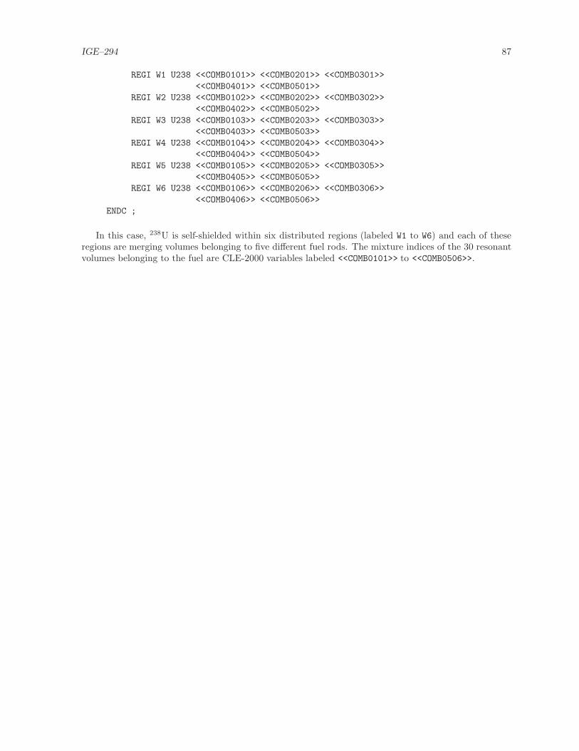
IGE–294 87

REGI W1 U238 <<COMB0101>> <<COMB0201>> <<COMB0301>>

<<COMB0401>> <<COMB0501>>


<<COMB0402>> <<COMB0502>>


<<COMB0403>> <<COMB0503>>


<<COMB0404>> <<COMB0504>>


<<COMB0405>> <<COMB0505>>


<<COMB0406>> <<COMB0506>>

ENDC ;

In this case, 238U is self-shielded within six distributed regions (labeled W1 to W6) and each of theseregions are merging volumes belonging to five different fuel rods. The mixture indices of the 30 resonantvolumes belonging to the fuel are CLE-2000 variables labeled <<COMB0101>> to <<COMB0506>>.

IGE–294 88

3.7 The ASM: module

We will now describe the assembly modules which can be used to prepare the group-dependent com-plete collision probability or the assembly matrices required by the flux solution module of DRAGON.The assembly module ASM: is generally called after a tracking module; it recovers tracking lengths andmaterial numbers from the sequential tracking file and then computes the collision probability or group–dependent system matrices under various normalizations. The calling specifications are:

Table 42: Structure (ASM:)

PIJNAM := ASM: [ PIJNAM ] LIBNAM TRKNAM [ TRKFIL ] :: (descasm)

where

PIJNAM character*12 name of asmpij data structure containing the system matrices. If PIJ-NAM appears on the RHS, the (descasm) information previously stored in PIJNAMis kept.

LIBNAM character*12 name of the macrolib or microlib data structure that contains themacroscopic cross sections (see Sections 3.1 and 3.2).

TRKNAM character*12 name of the tracking data structure containing the tracking (seeSection 3.4).


(descasm) structure containing the input data to this module (see Section 3.7.1).

3.7.1 Data input for module ASM:

Table 43: Structure (descasm)

[ EDIT iprint ][ ARM | PIJ | PIJK [ SKIP ][ NORM | ALBS ][ PNOR NONE | DIAG | GELB | HELI | NONL ]

][ ECCO ];

where


iprint index used to control the printing of this module. The amount of output produced by

IGE–294 89

this tracking module will vary substantially depending on the print level specified.

ARM keyword to specify that an assembly calculation is carried out without building thefull collision probability matrices. This option can only be used for a geometry trackedusing the SYBILT: (with EURYDICE-2 option) or MCCGT: module. By default, thePIJ option is used.

PIJ keyword to specify that the standard scattering-reduced collision probabilities must becomputed. This option cannot be used with the MCCGT: module. This is the defaultoption.

PIJK keyword to specify that both the directional and standard scattering-reduced collisionprobabilities must be computed. Moreover, the additional directional collision prob-ability matrix can only be used if HETE is activated in Section 3.8. Finally, the PIJK

option is only available for 2–D geometries analyzed with the operator EXCELT: withcollision probability option. By default, the PIJ option is used.

SKIP keyword to specify that only the reduced collision probability matrix pgij is to becomputed. In general, the scattering modified collision probability matrix pgs,ij is alsocomputed using:

pgs,ij =[

I − pgijΣg→gs0

]−1pgij

where Σg→gs0 is the within group isotropic scattering cross section. When available,

pgs,ij is used in the flux solution module in such a way that for the groups where thereis no up-scattering, the thermal iteration is automatically deactivated. In the casewhere the SKIP option is activated, the pgij matrix is used and thermal iterations arerequired in every energy group. Consequently, the total number of inner iterations isgreatly increased.

NORM keyword to specify that the scattering-reduced collision probability matrix is to benormalized in such a way as to eliminate all neutron loss (even if the region underconsideration has external albedo boundary conditions which should result in neutronloss). When used with a void boundary condition (zero reentrant current), this optionis equivalent to imposing a posteriori a uniform reentrant current.

ALBS keyword to specify that a consistent Selengut normalization of the scattering-reducedcollision probability matrix is to be used both for the flux solution module (seeSection 3.8) and in the equivalence calculation (see Section 3.9). This keyword re-sults in storing the scattering-reduced escape probabilities WiS in the record named’DRAGON-WIS’. For all the cases where this option is used, it is necessary to define ageometry with VOID external boundary conditions (see Section 3.3).

PNOR keyword to specify that the collision, leakage and escape probability matrices are to benormalized in such a way as to satisfy explicitly the neutron conservation laws. Thisoption compensates for the errors which will arise in the numerical evaluation of theseprobabilities and may result in non-conservative collision probability matrices. Thedefault option is now HELI while it was formerly GELB (Revision 3.03).

NONE keyword to specify that the probability matrices are not to be renormalized.

DIAG keyword to specify that only the diagonal element of the probability matrices will bemodified in order to insure the validity of the conservation laws.

GELB keyword to specify that the Gelbard algorithm will be used to normalize the collisionprobability matrices.[59]

HELI keyword to specify that the Helios algorithm will be used to normalize the collisionprobability matrices.[60]

NONL keyword to specify that a non-linear multiplicative algorithm will be used to normalizethe collision probability matrices.[59]

IGE–294 90

ECCO keyword used to compute the P1–scattering reduced collision probability or system ma-trices required by the ECCO isotropic streaming model. By default, this informationis not calculated.

IGE–294 91

3.8 The FLU: module

The FLU: module is used to solve the linear system of multigroup collision probability or responsematrix equations in DRAGON. Different types of solution are available, such as fixed source problem, fixedsource eigenvalue problem (GPT type) or different types of eigenvalue problems. The calling specificationsare:

Table 44: Structure (FLU:)

FLUNAM := FLU: [ FLUNAM ] PIJNAM LIBNAM TRKNAM [ TRKFIL ][ TRKFLP TRKGPT ] :: (descflu)

where

FLUNAM character*12 name of the fluxunk data structure containing the solution (L FLUX

signature). If FLUNAM appears on the RHS, the solution previously stored in FLU-NAM (flux and buckling) is used to initialize the new iterative process; otherwise, auniform unknown vector and a zero buckling are used.

PIJNAM character*12 name of the asmpij data structure containing the group-dependentsystem matrices (L PIJ signature, see Section 3.7).

LIBNAM character*12 name of the macrolib or microlib data structure that contains themacroscopic cross sections (L MACROLIB or L LIBRARY signature, see Sections 3.1 and 3.2).Module FLU: is performing a direct or adjoint calculation, depending if the adjoint flagis set to .false. or .true. in the STATE-VECTOR record of the macrolib.

TRKNAM character*12 name of the tracking data structure containing the tracking (L TRACK

signature, see Section 3.4).


TRKFLP character*12 name of the fluxunk data structure containing the unperturbed fluxused to decontaminate the GPT solution (L FLUX signature). This object is mandatoryif and only if “TYPE P” is selected.

TRKGPT character*12 name of the gpt data structure containing the GPT fixed sources(L GPT

signature). This object is mandatory if and only if “TYPE P” is selected.

(descflu) structure containing the input data to this module (see Section 3.8.1).

IGE–294 92

3.8.1 Data input for module FLU:

Table 45: Structure (descflu)

[ EDIT iprint ][ INIT OFF | ON ]TYPE N | S | P | K [ (descleak) ] | B | L (descleak) ][ EXTE [ maxout ] [ epsout ] ][ THER [ maxthr ] [ epsthr ] ] [ REBA [ OFF ] ][ UNKT [ epsunk ] ][ ACCE nlibre naccel ];

where


iprint index used to control the printing of this operator. The amount of output produced bythis operator will vary substantially depending on the print level specified.

OFF keyword to specify that the neutron flux is to be initialized with a flat distribution.

ON keyword to specify that the initial neutron flux distribution is to be recovered from FLU-NAM if present in the RHS arguments. Otherwise, the neutron flux is to be initializedwith a flat distribution.

TYPE keyword to specify the type of solution used in the flux operator.

N keyword to specify that no flux calculation is to be performed. This option is usuallyactivated when one simply wishes to initialize the neutron flux distribution and to storethis information in FLUNAM .

S keyword to specify that a fixed source problem is to be treated. Such problem can alsoinclude fission source contributions.

P keyword to specify that a fixed source eigenvalue problem (GPT type) is to be treated.Such problem includes fission source contributions in addition of GPT sources.

K keyword to specify that a fission source eigenvalue problem is to be treated. The eigen-value is then the effective multiplication factor with a fixed buckling. In this case, thefixed sources, if any is present on the macrolib or microlib data structure, are notused.

B keyword to specify that a fission source eigenvalue problem is to be treated. The eigen-value in this case is the critical buckling with a fixed effective multiplication factor. Thebuckling eigenvalue has meaning only in the case of a cell without leakages (see thestructure (descBC) in Section 3.3.2). It is also possible to use an open geometry withVOID boundary conditions provided it is closed by the ASM: module (see Section 3.7.1)using the keywords NORM or ALSB.

L keyword to specify that a non-multiplicative medium eigenvalue problem is to be treated.The eigenvalue in this case is the critical buckling with vanishing fission cross sections.The buckling eigenvalue has meaning only in the case of a cell without leakages (see thestructure (descBC) in Section 3.3.2). It is also possible to use an open geometry with

IGE–294 93

VOID boundary conditions provided it is closed by the ASM: module (see Section 3.7.1)using the keywords NORM or ALSB.

(descleak) structure describing the general leakage parameters options (see Section 3.8.2).

EXTE keyword to specify that the control parameters for the external iteration are to be mod-ified.

maxout maximum number of external iterations. The fixed default value for a case with noleakage model is maxout=2× nf − 1 where nf is the number of regions containing fuel.The fixed default value for a case with a leakage model is maxout=10× nf − 1.

epsout convergence criterion for the external iterations. The fixed default value is epsout=5.0×10−5.

THER keyword to specify that the control parameters for the thermal iterations are to bemodified.

maxthr maximum number of thermal iterations. The fixed default value is maxthr=2×ngroup-1(using scattering modified CP) or maxthr=4×ngroup-1 (using standard CP).

epsthr convergence criterion for the thermal iterations. The fixed default value is epsthr=5.0×10−5.

UNKT keyword to specify the flux error tolerance in the outer iteration.

epsunk convergence criterion for flux components in the outer iteration. The fixed default valueis epsunk=epsthr.

REBA keyword used to specify that the flux rebalancing option is to be turned on or off in thethermal iteration. By default (floating default) the flux rebalancing option is initiallyactivated. This keyword is required to toggle between the on and off position of the fluxrebalancing option.

OFF keyword used to deactivate the flux rebalancing option. When this keyword is absentthe flux rebalancing option is reactivated.

ACCE keyword used to modify the variational acceleration parameters. This option is active bydefault (floating default) with nlibre=3 free iterations followed by naccel=3 acceleratediterations.

nlibre number of free iterations per cycle of nlibre+naccel iterations.

naccel number of accelerated iterations per cycle of nlibre+naccel iterations. Variational accel-eration may be deactivated by using naccel=0.

3.8.2 Leakage model specification structure

Without leakage model, the multigroup flux ~φg of the collision probability method is obtained fromequation

~φg = Wg~Q∗g (3.1)

where Wg is the scattering reduced collision probability matrix and Q∗g is the fission and out-of-groupscattering source. This equation is modified by the leakage model. The leakage models PNLR, PNL, SIGSand ECCO can also be used with solutions techniques other than the collision probability method.

The (descleak) structure allows the following information to be specified:

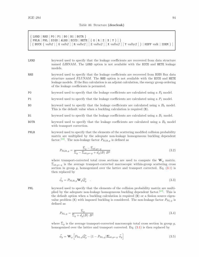
IGE–294 94

Table 46: Structure (descleak)

LKRD | RHS | P0 | P1 | B0 | B1 | B0TR PNLR | PNL | SIGS | ALBS | ECCO | HETE [ G | R | Z | X | Y ] [ BUCK valb2 | [ G valb2 ] [ R valbr2 ] [ Z valbz2 ] [ X valbx2 ] [ Y valby2 ] | KEFF valk | IDEM ]

LKRD keyword used to specify that the leakage coefficients are recovered from data structurenamed LIBNAM . The LKRD option is not available with the ECCO and HETE leakagemodels.

RHS keyword used to specify that the leakage coefficients are recovered from RHS flux datastructure named FLUNAM . The RHS option is not available with the ECCO and HETE

leakage models. If the flux calculation is an adjoint calculation, the energy group orderingof the leakage coefficients is permuted.

P0 keyword used to specify that the leakage coefficients are calculated using a P0 model.

P1 keyword used to specify that the leakage coefficients are calculated using a P1 model.

B0 keyword used to specify that the leakage coefficients are calculated using a B0 model.This is the default value when a buckling calculation is required (B).

B1 keyword used to specify that the leakage coefficients are calculated using a B1 model.

B0TR keyword used to specify that the leakage coefficients are calculated using a B0 modelwith transport correction.

PNLR keyword used to specify that the elements of the scattering modified collision probabilitymatrix are multiplied by the adequate non-leakage homogeneous buckling dependentfactor.[68]. The non-leakage factor PNLR,g is defined as

PNLR,g =Σg − Σs0,g←g

Σg − Σs0,g←g + dg(B) B2(3.2)

where transport-corrected total cross sections are used to compute the Wg matrix.Σs0,g←g is the average transport-corrected macroscopic within-group scattering crosssection in group g, homogenized over the lattice and transport corrected. Eq. (3.1) isthen replaced by

~φg = PNLR,gWg~Q∗g . (3.3)

PNL keyword used to specify that the elements of the collision probability matrix are multi-plied by the adequate non-leakage homogeneous buckling dependent factor.[68]. This isthe default option when a buckling calculation is required (B) or a fission source eigen-value problem (K) with imposed buckling is considered. The non-leakage factor PNL,g isdefined as

PNL,g =Σg

Σg + dg(B) B2(3.4)

where Σg is the average transport-corrected macroscopic total cross section in group g,homogenized over the lattice and transport corrected. Eq. (3.1) is then replaced by

~φg = Wg

[

PNL,g~Q∗g − (1− PNL,g)Σs0,g←g

~φg

]

(3.5)

IGE–294 95

where Σs0,g←g = diagΣs0,i,g←g ; ∀i and the total cross sections used to compute theWg matrix are also transport-corrected.

It is important to note that that the PNLR option reduces to the PNL option in caseswhere no scattering reduction is performed. Scattering reduction can be avoided inmodule ASM: by setting PIJ SKIP (See Section 3.7.1).

SIGS keyword used to specify that an homogeneous buckling correction is to be applied on thediffusion cross section (Σs − dB2). Eq. (3.1) is then replaced by

~φg = Wg

[

~Q∗g − dg(B) B2 ~φg

]

(3.6)

where transport-corrected total cross sections are used to compute the Wg matrix. Thisis the so called DIFFON method used in the APOLLO-family of thermal lattice codes.

ALBS keyword used to specify that an homogeneous buckling contribution is introduced bya group dependent correction of the albedo.[69] This leakage model is restricted to thecollision probability method. It is then necessary to define the geometry with an externalboundary condition of type VOID (see Section 3.3.2) and to close the region in moduleASM: using the ALBS option (see Section 3.7.1). Eq. (3.1) is then replaced by

~φg = Wg~Q∗g − [I+WgΣs0,g←g] dg(B) B2 γ PiS,g (3.7)

where PiS,g = PiS,g ; i = 1, I is the array of escape probabilities in the open geometryand where

γ =

∑

j

Vjφj,g

∑

j

Vjφj,gPjS,g. (3.8)

ECCO keyword used to perform an ECCO–type leakage calculation taking into account isotropicstreaming effects. This method introduces an heterogeneous buckling contribution asa group dependent correction to the source term.[61, 62] It is then necessary to set thekeyword ECCO in module ASM: (see Section 3.7.1). In the P1 non–consistent case, Eq. (3.1)is then replaced by

~ϕg = Wg

(

~Q∗g −B2 i ~JgB

)

(3.9)

i ~JgB

= Xg

1

3~ϕg +

∑

h 6=g

Σs1,g←hi ~JhB

(3.10)

where i ~Jj,g/B is the multigroup fundamental current, Σs1,g←h = diagΣs1,i,g←h ; ∀iand where

Xg = [I− pg Σs1,g←g]−1pg . (3.11)

HETE keyword used to perform a TIBERE–type leakage calculation taking into account anisotropicstreaming effects. This method introduces an heterogeneous buckling contribution as agroup dependent correction to the source term.[63, 64] The heterogeneous buckling con-tribution is introduced in the Bn model using directional collision probabilities (PIJKmethod). It is then necessary to set the keyword PIJK in module ASM: (see Section 3.7.1).

IGE–294 96

G keyword used to specify that the buckling search will assume all directional buckling tobe identical (floating default option).

R keyword used to specify that a radial buckling search will be considered assuming animposed z-direction buckling.

Z keyword used to specify that a z-direction buckling search will be considered assumingan imposed x-direction and y-direction buckling.

X keyword used to specify that a x-direction buckling search will be considered assumingan imposed y-direction and z-direction buckling.

Y keyword used to specify that a y-direction buckling search will be considered assumingan imposed x-direction and z-direction buckling.

BUCK keyword used to specify the initial (for a buckling eigenvalue problem) or fixed (for aeffective multiplication constant eigenvalue problem) buckling.

G keyword used to specify that the buckling in the x-direction, y-direction and z-directionare to be initialized to valb2/3 (floating default).

R keyword used to specify that the buckling in the x-direction, and y-direction are to beinitialized to valbr2/2.

Z keyword used to specify that the buckling in the z-direction, is to be initialized to valbz2 .

X keyword used to specify that the buckling in the x-direction, is to be initialized to valbx2 .

Y keyword used to specify that the buckling in the y-direction, is to be initialized to valby2 .

valb2 value of the fixed or initial total buckling in cm−2. The floating default value is

valb2 = valbx2 + valby2 + valbz2 .

valbr2 value of the fixed or initial radial buckling in cm−2. The floating default value is

valbr2 = valbx2 + valby2 .

valbz2 value of the fixed or initial z-direction buckling in cm−2. The floating default value isvalbz2=0.0 cm−2. If valb2 is specified then valbz2=valb2/3.

valbx2 value of the fixed or initial z-direction buckling in cm−2. The floating default value isvalbx2=0.0 cm−2. If valb2 is specified then valbx2=valb2/3. If valbr2 is specified thenvalbx2=valbr2/2.

valby2 value of the fixed or initial z-direction buckling in cm−2. The floating default value isvalby2=0.0 cm−2. If valb2 is specified then valby2=valb2/3. If valbr2 is specified thenvalby2=valbr2/2.

KEFF keyword used to specify the fixed (for a buckling eigenvalue problem) effective multipli-cation constant.

valk value of the fixed effective multiplication constant. The fixed default value is valk=1.0.

IDEM keyword used to specify that the initial (for a buckling eigenvalue problem) or fixed (fora effective multiplication constant eigenvalue problem) buckling is to be read from thedata structure LIBNAM .

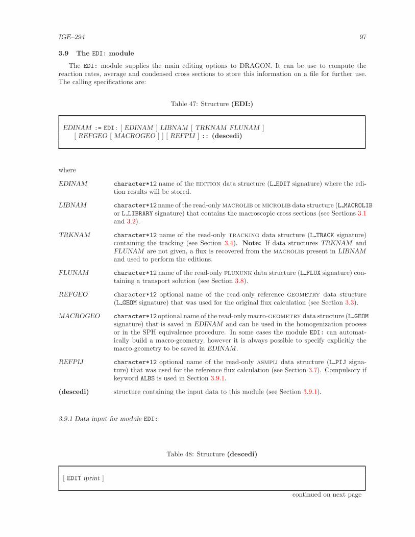
IGE–294 97

3.9 The EDI: module

The EDI: module supplies the main editing options to DRAGON. It can be use to compute thereaction rates, average and condensed cross sections to store this information on a file for further use.The calling specifications are:

Table 47: Structure (EDI:)

EDINAM := EDI: [ EDINAM ] LIBNAM [ TRKNAM FLUNAM ][ REFGEO [ MACROGEO ] ] [ REFPIJ ] :: (descedi)

where

EDINAM character*12 name of the edition data structure (L EDIT signature) where the edi-tion results will be stored.

LIBNAM character*12 name of the read-onlymacrolib ormicrolib data structure (L MACROLIB

or L LIBRARY signature) that contains the macroscopic cross sections (see Sections 3.1and 3.2).

TRKNAM character*12 name of the read-only tracking data structure (L TRACK signature)containing the tracking (see Section 3.4). Note: If data structures TRKNAM andFLUNAM are not given, a flux is recovered from the macrolib present in LIBNAMand used to perform the editions.

FLUNAM character*12 name of the read-only fluxunk data structure (L FLUX signature) con-taining a transport solution (see Section 3.8).

REFGEO character*12 optional name of the read-only reference geometry data structure(L GEOM signature) that was used for the original flux calculation (see Section 3.3).

MACROGEO character*12 optional name of the read-only macro-geometry data structure (L GEOM

signature) that is saved in EDINAM and can be used in the homogenization processor in the SPH equivalence procedure. In some cases the module EDI: can automat-ically build a macro-geometry, however it is always possible to specify explicitly themacro-geometry to be saved in EDINAM .

REFPIJ character*12 optional name of the read-only asmpij data structure (L PIJ signa-ture) that was used for the reference flux calculation (see Section 3.7). Compulsory ifkeyword ALBS is used in Section 3.9.1.

(descedi) structure containing the input data to this module (see Section 3.9.1).

3.9.1 Data input for module EDI:

Table 48: Structure (descedi)

[ EDIT iprint ]


IGE–294 98

Structure (descedi) continued from last page

[ UPS ][ MERG NONE | COMP | GEO | HMIX |

CELL [ SYBIL | EXCELL | NXT | DEFAULT ] [ REMIX (imixm2(ii),ii=1,nbmix2) ] |REGI (iregm(ii),ii=1,nregio) |MIX [ (imixm(ii),ii=1,nbmix) ] ]

[ TAKE REGI (iregt(ii),ii=1,nregio) |MIX (imixt(ii),ii=1,nbmix) ]

[ P0W | P1W L | P1W T ][ COND [ NONE | ( icond(ii), ii=1,ngcond) | ( energy(ii), ii=1,ngcond) ] ][ MICR [ ALLX ] [ ISOTXS [ ASCII ] ] ALL | RES | nis (HISO(i),i=1,nis)

[ REAC nreac (HREAC(i),i=1,nreac) ] ][ ACTI [ ISOTXS [ ASCII ] ] NONE | (imixa(ii),ii=1,nbmix) ] [ SAVE [ ON DIRN | idirn ] ][ PERT ][ STAT ALL | RATE | FLUX | DELS [ REFE DIRO | idiro ] ][ NOHF ] [ NBAL ][ MAXR maxpts ][ DIRE | PROD ][ MGEO MACGEO ][ NADF | ALBS | JOUT |

[[ ADF TYPE REGI (ireg(ii),ii=1,iimax) ENDR | MIX (imix(ii),ii=1,iimax) ENDM ]] ]

where


iprint index used to control the printing of this module. The iprint parameter is importantfor adjusting the amount of data that is printed by this calculation step:

• iprint=0 results in no output;

• iprint=1 results in the average and integrated fluxes being printed (floating de-fault);

• iprint=2 results in the reaction rates being printed;

• iprint=3 is identical to the previous option, but the condensed and/or homoge-nized vectorial cross sections are also printed;

• iprint=4 is identical to the previous option, but the condensed and/or homoge-nized transfer cross sections are also printed.

UPS keyword to specify that the reaction rates and the condensed and/or homogenizedcross sections are corrected so as to eliminate up-scattering. This option is useful forreactor analysis codes which cannot take into account such cross sections.

NONE keyword to deactivate the homogeneization or the condensation.

MERG keyword to specify that the neutron flux is to be homogenized over specified regionsor mixtures.

REGI keyword to specify that the homogenization of the neutron flux will take place over thefollowing regions. Here nregio≤maxreg with maxreg the maximum number of regionsfor which solutions were obtained.

IGE–294 99

iregm array of homogenized region numbers to which are associated the old regions. In theediting routines a value of iregm=0 allows the corresponding region to be neglected.

MIX keyword to specify that the homogenization of the neutron flux will take place overthe following mixtures. Here we must have nbmix≤maxmix where maxmix is themaximum number of mixtures in the macroscopic cross section library.

imixm array of homogenized region numbers to which are associated the material mixtures.In the editing routines a value of imixm=0 allows the corresponding isotopic mixturesto be neglected. For a mixture in this library which is not used in the geometry oneshould insert a value of 0 for the new region number associated with this mixture. Bydefault, if MIX is set and imixm is not set, imixm(ii)=ii is assumed.

COMP keyword to specify that the a complete homogenization is to take place.

GEO keyword to specify that a geometry equivalence procedure (equigeom) is to be used.Merging indices are automatically computed by comparing the reference geometry RE-FGEO with the macro-geometryMACROGEO. This capability is limited to EXCELL–type reference geometries.

HMIX keyword to specify that the homogenization region will be selected using the informa-tion provided by the HMIX option in the GEO: module (see Section 3.3.4). In this case,all the regions associated with a virtual homogenization mixture will be homogenized.If the virtual homogenization mixtures were not defined in the geometry, the real mix-tures are used instead (see MIX keyword in Section 3.3.4). This option is valid only forNXT: based tracking data structure (this option uses the information stored on thereference TRKNAM data structure).

CELL keyword to specify that the a cell-by-cell homogenization (with or without SPH equiva-lence) is to take place. The macro-geometry and the merging indices are automaticallycomputed and the macro-geometry named MACRO-GEOM is created on the root directoryof EDINAM . This capability is limited to reference geometries previously tracked byEURYDICE (see Section 3.4.1) or NXT (see Section 3.4.3).

SYBIL the macro-geometry produced by CELL is tracked by SYBILT: module.

EXCELL the macro-geometry produced by CELL is tracked by EXCELT: module.

NXT the macro-geometry produced by CELL is tracked by NXT: module.

DEFAULT the macro-geometry produced by CELL is tracked by another module (default option).

REMIX the cell-by-cell homogenization produced by option CELL is further homogenized ac-cording to imixm2 indices. This option is useful to integrate the assembly gap intothe boundary cells. By default, one homogenized region is created for each cell of themacro-geometry.

imixm2 array of rehomogenized region numbers to which are associated the regions indicescreated after the cell-by-cell homogenization was performed. In the editing routines avalue of imixm2=0 allows the corresponding cell region to be neglected. Here, nbmix2is equal to the number of cells in the macro-geometry.

TAKE keyword to specify that the neutron flux is to be edited over specified regions ormixtures.

REGI keyword to specify that the editing of the neutron flux will take place over the followingregions. Here nregio≤maxreg with maxreg the maximum number of regions for whichsolutions were obtained.

iregt regions where the editing will take place. The new region numbers associated withthese editing regions are numbered sequentially.

IGE–294 100

MIX keyword to specify that the editing of the neutron flux will take place over the followingmixtures. Here we must have nbmix≤maxmix where maxmix is the maximum numberof mixtures in the macroscopic cross section library.

imixt mixtures where the editing will take place. Each mixture set here must exists in thereference geometry.

P0W keyword to specify that the P1 information is to be homogenized and condensed usingthe scalar flux. This is the default option.

P1W L keyword to specify that the P1 information is to be homogenized and condensed usinga current recovered from a consistent P1 or from a consistent heterogeneous B1 model.

P1W T keyword to specify that the P1 information is to be homogenized and condensed usingthe Todorova flux[93], defined as

φ1(r, E) =φ(r, E)

Σi(E)− Σs1,i(E)

where Σi(E) and Σs1,i(E) are the macroscopic total and P1 scattering cross sectionsin the mixture i containing the point r.

COND keyword to specify that a group condensation of the flux is to be performed.

icond array of increasing energy group limits that will be associated with each of the ngcondcondensed groups. The final value of icond will automatically be set to ngroup whilethe values of icond>ngroup will be droped from the condensation. We must havengcond≤ngroup. By default, if COND is set and icond is not set, all energy groups arecondensed together.

energy array of decreasing energy limits (in eV) that will be associated with each of the ngcondcondensed groups. We must have ngcond≤ngroup+1 . Note that if an energy limit islocated between two energy groups, the condensation group will include this associatedenergy group. In the case where two energy limits fall within the same energy groupthe lowest energy will be droped. Finally the maximum and minimum energy limitscan be skipped since they will be taken automatically from the information availablein the library.

MICR keyword to specify that the condensation and homogenization procedure will be usedto associate microscopic cross sections to the isotopes present in the homogenizedregions. The macroscopic cross sections and the diffusion coefficients are weighted bythe multigroup fluxes appearing in the regions where the isotopes are present. Theresulting nuclear properties are saved on EDINAM when the SAVE keyword is present.

ALLX keyword used to register the region number of each isotope before merging, in the em-bedded library. The homogeneized information is therefore registered for each isotopein the merging region, as depicted by the formulas below. This procedure is usefulto produce particular databases, in order to perform micro-depletion calculations indiffusion with DONJON.

ALL keyword to specify that all the isotopes present in the homogenized region are to bekept individual and processed.

RES keyword to specify that all the isotopes present in the homogenized region will bemerged as a single residual isotope.

nis number of isotopes present in the homogenized region to be processed.

HISO array of character*8 isotopes alias names to be processed.

REAC keyword to specify the reaction names to be included in the output microlib. Bydefault, all available reactions are included in the output microlib.

IGE–294 101

nreac number of reactions to be included in the output microlib.

HREAC array of character*8 reaction names to be included in the output microlib.

ACTI keyword to specify that microscopic activation data will be edited for the isotopesassociated with the specified mixture. This information correspond to the microscopiccross section associated with each isotope in a given macro-group and macro-regionassuming a concentration for this isotope of 1.0 ×cm−3 in each region. This keywordis followed by nacti material mixture indices, where nacti≤maxmix.

NONE keyword to specify that no isotope present in the homogenized region is to be used asactivation data.

imixa array of material mixture indices which contains the isotopes for which activation datais to be generated. nmix≤maxmix. Even mixture not used in the geometry can beconsidered here.

ISOTXS keyword to specify that the set of microscopic cross section generated by the MICR andACTI command will also be saved on a microscopic group neutron cross section libraryin the ISOTXS-IV format. This will generate a file for each final region specifiedby the TAKE or MERG keyword, numbered consecutively (IFILE). The name of the file(NISOTXS) is built using the command

WRITE(NISOTXS,’(A6,I6.6)’) ’ISOTXS’,IFILE

ASCII keyword to specify that the ISOTXS file is created in ascii format. By default, it iscreated in binary format.

SAVE keyword to specify that the fluxes, the macroscopic and microscopic cross sections andthe volumes corresponding to homogenized regions are to be saved on EDINAM . Amacrolib is store on a subdirectory of edition.

ON keyword to specify on which directory of EDINAM this information is to be stored.

DIRN name of the directory on which the above information is to be stored.

idirn number associated with a directory of EDINAM on which the above information is tobe stored. To each number idirn is associated a directory name CDIRN=’REF-CASE’//CN

where CN is a character*4 variable defined by WRITE(CN,’(I4)’) idirn.

PERT keyword to specify that first order perturbations for the microscopic cross sections areto be saved on EDINAM .

STAT keyword to specify that a comparison between the current and a reference set of reac-tion rates and/or integrated fluxes is to be performed.

ALL keyword to specify that the relative differences in the reaction rates and the integratedfluxes are to be printed.

RATE keyword to specify that the relative differences in the reaction rates are to be printed.

FLUX keyword to specify that the relative differences in the integrated fluxes are to beprinted.

DELS keyword to specify that the absolute differences in the macroscopic cross section areto be printed.

REFE keyword to specify the directory of EDINAM where the reference data requires forthe comparison is stored. When this keyword is absent, the last reaction rates andintegrated fluxes saved on EDINAM are used.

IGE–294 102

DIRO name of the directory from which the reference information is taken.

idiro number associated with an directory of EDINAM on which the reference informationis stored. To each number idirn is associated a the directory CDIRN=’REF-CASE’//CN

where CN is a character*4 variable defined by WRITE(CN,’(I4)’) idirn.

NOHF keyword to suppress the calculation and edition of the H-factors (sum of all the crosssections producing energy times the energy produced by each reaction). Note thatthis calculation may be time-consuming. By default, the H-factors are computed andedited if keyword DEPL and associated data is set in module LIB:.

NBAL keyword to specify the editing of the four factors computed from a group balance. Inthis case, the user must specify explicitly a three group condensation.

MAXR keyword to specify the number of components in region-related dynamically allocatedarrays. If the default value is not sufficient, an error message is issued.

maxpts user-defined maximum number of components.

DIRE use the direct flux to perform homogenization or/and condensation (default value).

PROD use the product of the direct and adjoint flux to perform homogenization or/andcondensation. This option is used only in specialized applications such as in the clio

perturbative analysis formula.[92] The homogenization and condensation equations arepresented in Sect. 3.9.3. Note: The FLUNAM object must contain both an adjointand a direct flux solution.

MGEO keyword to define the name of the macro-geometry, which must appear among theRHS. The macro-geometry is recovered automatically by interface modules such asCOMPO: (see Section 3.14) or manually by a CLE-2000 statement such as

GEONAM := EDINAM :: STEP UP ’MACRO-GEOM’ ;

where GEONAM and EDINAM are L GEOM and L EDIT LCM objects, respectively.

MACGEO character*12 name of the macro-geometry.

NADF keyword to desactivate boundary editions.

ALBS keyword to specify that the boundary flux is to be obtained from relation φsurf =4Jout/S where Jout is the outgoing interface current. The albedo of the geometry areto be taken into account in the complete homogenization process. Thus the MERG andCOMP options must be specified. The boundary fluxes are obtained from a calculationusing the collision probabilities. This option requires a geometry with VOID (see Sec-tion 3.3.2) external boundary conditions to be closed using ALBS in module ASM: (seeSection 3.7.1).[69]

JOUT keyword to specify that the boundary flux is to be obtained from relation φsurf =4Jout/S where Jout is the outgoing interface current. The outgoing interface current isrecovered by direct homogenization and condensation of the flux unknown componentscorresponding to external boundary and used with the current iteration method inEurydice. This keyword is only compatible if a SYBILT: tracking is used and if keywordARM is set in module ASM: (see Section 3.7.1).

ADF keyword to specify that boundary editions are required. Averaged fluxes are computedover boundary regions.

TYPE character*4 name of the boundary edit corresponding to regions ireg or mixturesimix. Any user-defined name can be used, but some standard names are recognizedby module SPH (see Section 3.11.2). Standard names are: = FD C: corner flux edition;= FD B: surface (assembly gap) flux edition; = FD H: row flux edition. These are thefirst row of surrounding cells in the assembly.

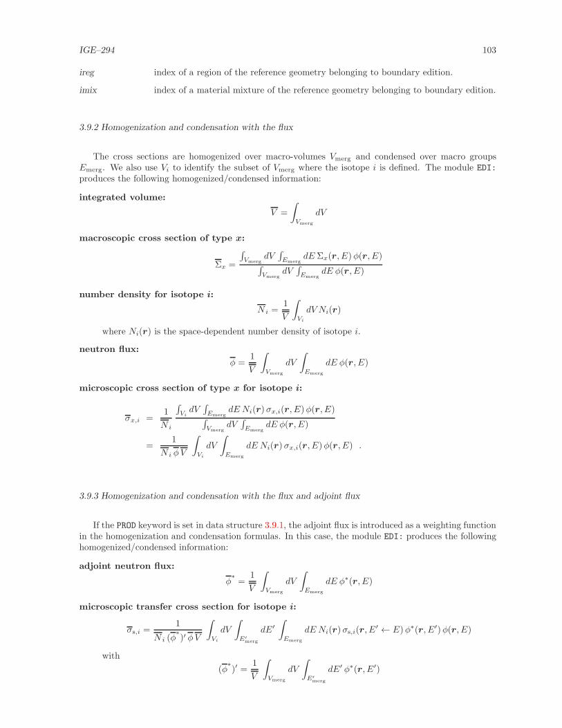
IGE–294 103

ireg index of a region of the reference geometry belonging to boundary edition.

imix index of a material mixture of the reference geometry belonging to boundary edition.

3.9.2 Homogenization and condensation with the flux

The cross sections are homogenized over macro-volumes Vmerg and condensed over macro groupsEmerg. We also use Vi to identify the subset of Vmerg where the isotope i is defined. The module EDI:

produces the following homogenized/condensed information:

integrated volume:

V =

∫

Vmerg

dV

macroscopic cross section of type x:

Σx =

∫

VmergdV∫

EmergdE Σx(r, E)φ(r, E)

∫

VmergdV∫

EmergdE φ(r, E)

number density for isotope i:

N i =1

V

∫

Vi

dV Ni(r)

where Ni(r) is the space-dependent number density of isotope i.

neutron flux:

φ =1

V

∫

Vmerg

dV

∫

Emerg

dE φ(r, E)

microscopic cross section of type x for isotope i:

σx,i =1

N i

∫

VidV∫

EmergdE Ni(r)σx,i(r, E)φ(r, E)

∫

VmergdV∫

EmergdE φ(r, E)

=1

N i φV

∫

Vi

dV

∫

Emerg

dE Ni(r)σx,i(r, E)φ(r, E) .

3.9.3 Homogenization and condensation with the flux and adjoint flux

If the PROD keyword is set in data structure 3.9.1, the adjoint flux is introduced as a weighting functionin the homogenization and condensation formulas. In this case, the module EDI: produces the followinghomogenized/condensed information:

adjoint neutron flux:

φ∗=

1

V

∫

Vmerg

dV

∫

Emerg

dE φ∗(r, E)

microscopic transfer cross section for isotope i:

σs,i =1

N i (φ∗)′ φV

∫

Vi

dV

∫

E′

merg

dE′∫

Emerg

dE Ni(r)σs,i(r, E′ ← E)φ∗(r, E′)φ(r, E)

with

(φ∗)′ =

1

V

∫

Vmerg

dV

∫

E′

merg

dE′ φ∗(r, E′)

IGE–294 104

microscopic cross section of type x 6= f for isotope i:

σx,i =1

N i φ∗φV

∫

Vi

dV

∫

Emerg

dE Ni(r)σx,i(r, E)φ∗(r, E)φ(r, E)

microscopic ν times fission cross section for isotope i:

νσf,i =1

N i φV

∫

Vi

dV

∫

Emerg

dE Ni(r) νσf,i(r, E)φ(r, E)

fission spectra for isotope i:

χi =1

N i φ∗V

∫

Vi

dV

∫

Emerg

dE Ni(r)χi(r, E)φ∗(r, E) .

Both the macrolib and microlib information is affected by the adjoint weighting. However, users shouldbe advised that this operation may have some undesirable effects on the fission spectrum normalization.Its use must therefore be limited to specialized applications where the adjoint weighting is theoreticallyrequired. This is the case, for example, with the clio perturbative analysis method.[92]

IGE–294 105

3.10 The EVO: module

The EVO: module performs the burnup calculations. The depletion equations for the various isotopeof the microlib are solved using the burnup chains also present in the microlib. Both in-core andout-of-core calculations can be considered. For in-core depletion calculations, one assumes linear fluxvariation over each irradiation period (time stage). The initial (and possibly final) flux distributionsare recovered from previous FLU: calculations. In-core depletion can be performed at constant flux orconstant power (expressed in MW/Tonne of initial heavy elements) but these values can undergo stepvariations from one time stage to another. All the information required for successive burnup calculationis stored on the PyLCM burnup data structure. Thus it is possible at any point in time to return to aprevious time step and restart the calculations.

In each burnup mixture of the unit cell, the depletion of K isotopes over a time stage (t0, tf ) followsthe following equation:

dNk

dt+Nk(t) Λk(t) = Sk(t) ; k = 1,K (3.12)

with

Λk(t) = λk + 〈σa,k(t)φ(t)〉 , (3.13)

Sk(t) =

L∑

l=1

Ykl 〈σf,l(t)φ(t)〉 Nl(t) +

K∑

l=1

mkl(t) Nl(t) , (3.14)

〈σx,l(t)φ(t)〉 =

∫ ∞

0

σx,l(u)φ(t, u)du (3.15)

and

σx,k(t, u)φ(t, u) = σx,k(t0, u)φ(t0, u) +σx,k(tf , u)φ(tf , u)− σx,k(t0, u)φ(t0, u)

tf − t0(t− t0) (3.16)

where

K = number of depleting isotopes

L = number of fissile isotopes producing fission products

Nk(t) = time dependant number density for k-th isotope

λk = radioactive decay constant for k-th isotope

σx,k(t, u) = time and lethargy dependant microscopic cross section for nuclear reaction x on

k-th isotope. x=a, x=f and x=γ respectively stands for absorption, fission and

radiative capture cross sections

φ(t, u) = time and lethargy dependant neutron flux

Ykl = fission yield for production of fission product k by fissile isotope l

mkl(t) = radioactive decay constant or 〈σx,l(t)φ(t)〉 term for production of isotope k by

isotope l.

Depleting isotopes with Λk(t0) [tf − t0] ≥valexp and Λk(tf ) [tf − t0] ≥valexp are considered to be atsaturation. They are described by making dNk

dt = 0 in Eq. (3.12) to obtain

Nk(t) =Sk(t)

Λk(t); if k is at saturation. (3.17)

If the keyword SAT is set, beginning-of-stage and end-of-stage Dirac contributions are added to theprevious equation:

Nk(t) =1

Λk(t)[aδ(t− t0) + Sk(t) + bδ(t− tf )] ; if k is at saturation (3.18)

IGE–294 106

where a and b are chosen in order to satisfy the time integral of Eq. (3.12):

Nk(t+f )−Nk(t

−0 ) +

∫ t+f

t−0

Nk(t) Λk(t) dt =

∫ t+f

t−0

Sk(t) dt (3.19)

It is numerically convenient to chose the following values of a and b:

a = Nk(t−0 )−

Sk(t+0 )

Λk(t+0 )

(3.20)

and

b =Sk(t

+0 )

Λk(t+0 )−

Sk(t+f )

Λk(t+f )

(3.21)

The numerical solution techniques used in the EVO: module are the following. Very short periodisotopes are taken at saturation and are solved apart from non-saturating isotopes. If an isotope is takenat saturation, all its parent isotopes, other than fissiles isotopes, are also taken at saturation. Isotopes atsaturation can procuce daughter isotopes using decay and/or neutron-induced reactions.

The lumped depletion matrix system containing the non-saturating isotopes is solved using either afifth order Cash-Karp algorithm or a fourth order Kaps-Rentrop algorithm[74], taking care to perform allmatrix operations in sparse matrix algebra. Matrices [mkl(t0)] and [mkl(tf )] are therefore representedin diagonal banded storage and kept apart from the yield matrix [Ykl]. Every matrix multiplication orlinear system solution is obtained via the LU algorithm.

The solution of burnup equations is affected by the flux normalization factors. DRAGON can performout-of-core or in-core depletion with a choice between two normalization techniques:

1. Constant flux depletion. In this case, the lethargy integrated fluxes at beginning-of-stage andend-of-stage are set to a constant F :

∫ ∞

0

φ(t0, u)du =

∫ ∞

0

φ(tf , u)du = F (3.22)

2. Constant power depletion. In this case, the power released per initial heavy element at beginning-of-stage and end-of-stage are set to a constant W .

K∑

k=1

[

κf,k 〈σf,k(t0)φ(t0)〉+ κγ,k 〈σγ,k(t0)φ(t0)〉]

Nk(t0) =

K∑

k=1

[

κf,k 〈σf,k(tf )φ(tf )〉+ κγ,k 〈σγ,k(tf )φ(tf )〉]

Nk(tf ) = C0 W (3.23)

where

κf,k = energy (MeV) released per fission of the fissile isotope k

κγ,k = energy (MeV) released per radiative capture of isotope k

C0 = conversion factor (MeV/MJ) multiplied by the mass of initial heavy elements

expressed in metric tonnes

The end-of-stage power is function of the number densities Nk(tf ); a few iterations will thereforebe required before the end-of-stage power released can be set equal to the desired value. Note thatthere is no warranties that the power released keep its desired value at every time during the stage;only the beginning-of-stage and end-of-stage are set.

IGE–294 107

Whatever the normalisation technique used, DRAGON compute the exact burnup of the unit cell (inMW per tonne of initial heavy element) by adding an additional equation in the depletion system. Thisvalue is the local parameter that should be used to tabulate the output cross sections.

The general format of the data which is used to control the execution of the EVO: module is thefollowing:

Table 49: Structure (EVO:)

BRNNAM MICNAM := EVO:

[ BRNNAM ] MICNAM | OLDMIC [ FLUNAM TRKNAM | POWNAM ]:: (descevo)

where

BRNNAM character*12 name of the burnup data structure that will contain the depletionhistory as modified by the depletion module. If BRNNAM appears on both LHS andRHS, it is updated; otherwise, it is created.

MICNAM character*12 name of the microlib containing the microscopic cross sections at savepoint xts. MICNAM is modified to include an embedded macrolib containing theupdated macroscopic cross sections at set point xtr. If MICNAM appears on bothLHS and RHS, it is updated; otherwise, the internal library OLDMIC is copied inMICNAM and MICNAM is updated. It is possible to assign different microlib todifferent save points of the depletion calculation. In this case, the microscopic reactionrates will be linearly interpolated/extrapolated between points xti and xtf.

OLDMIC character*12 name of a read-only microlib that is copied in MICNAM .

FLUNAM character*12 name of a read-only fluxunk at save point xts. This informationis used for in-core depletion cases. This information is not required for out-of-coredepletion cases. Otherwise, it is mandatory

TRKNAM character*12 name of a read-only tracking constructed for the depleting geometryand consistent with object FLUNAM .

POWNAM character*12 name of a read-only power object (generated by DONJON) at savepoint xts. This information is used for micro-depletion cases.

(descevo) structure containing the input data to this module (see Section 3.10.1).

For the in-core depletion cases, the tracking tracking data structure on which FLUNAM is based,is automatically recovered in read-only mode from the generalized driver dependencies.

3.10.1 Data input for module EVO:

Table 50: Structure (descevo)

[ EDIT iprint ]


IGE–294 108

Structure (descevo) continued from last page

[ SAVE xts S | DAY | YEAR FLUX flux | POWR fpower | W/CC apower | NOSA ][ EPS1 valeps1 ] [ EPS2 valeps2 ] [ EXPM valexp | SATOFF ][ H1 valh1 ] [ RUNG | KAPS ][ TIXS | TDXS ] [ NOEX | EXTR ] [ NOGL | GLOB ] [ NSAT | SAT ] [ NODI | DIRA ][ FLUX FLUX | FLUX MAC | FLUX POW ] [ CHAIN | PIFI ][ DEPL xti xtf | dxt S | DAY | YEAR COOL | FLUX flux | POWR fpower | W/CC apower | KEEP ][ SET xtr S | DAY | YEAR ][ MIXB [[ mixbrn ]] ] [ MIXP [[ mixpwr ]] ];

where


iprint index used to control the printing of the module. The amount of output produced bythis tracking module will vary substantially depending on the print level specified.

SAVE keyword to specify that the current isotopic concentration and the microscopic reactionrates resulting from the last transport calculation will be normalized and stored onBRNNAM in a sub-directory corresponding to a specific time. By default this data isstored at a time corresponding to xti.

NOSA keyword to specify that the current isotopic concentration and the results of the lasttransport calculation will not be stored on BRNNAM . By default this data is stored ata time corresponding to xti.

SET keyword used to recover the isotopic concentration already stored on BRNNAM from asub-directory corresponding to a specific time. By default this data is recovered from atime corresponding to xtf .

DEPL keyword to specify that a burnup calculation between an initial and a final time must beperformed. In the case where the SAVE keyword is absent, the initial isotopic concentra-tion will be stored on BRNNAM on a sub-directory corresponding to the initial time. Ifthe SET keyword is absent, the isotopic concentration corresponding to the final burnuptime will be used to update MICNAM.

xti initial time associated with the burnup calculation. The name of the sub-directory wherethis information is stored will be given by ‘DEPL-DAT’//CNN where CNN is a character*4

variable defined by WRITE(CNN,’(I4.4)’) INN where INN is an index associated withthe time xti. The initial values are recovered from this sub-directory in BRNNAM .

xtf end of time for the burnup calculation. The results of the isotopic depletion calculationsare stored in the tables associated with a sub-directory whose name is constructed in thesame manner as the xti input.

dxt time interval for the burnup calculation. The initial time xti in this case is taken as thefinal time reached at the last depletion step. If this is the first depletion step, xti = 0.

xts time associated with the last transport calculation. The name of the sub-directory wherethis information is to be stored is constructed in the same manner as the for xti input.By default (fixed default) xts=xti.

xtr time associated with the next flux calculation. The name of the sub-directory where thisinformation is to be stored is constructed in the same manner as for the xti input. Bydefault (fixed default) xtr=xtf .

IGE–294 109

S keyword to specify that the time is given in seconds.

DAY keyword to specify that the time is given in days.

YEAR keyword to specify that the time is given in years.

COOL keyword to specify that a zero flux burnup calculation is to be performed.

FLUX keyword to specify that a constant flux burnup calculation is to be performed.

flux flux expressed in cm−2s−1.

POWR keyword to specify that a constant fuel power depletion calculation is to be performed.The energy released outside the fuel (e.g., by (n,γ) reactions) is not taken into accountin the flux normalization, unless the GLOB option is set.

fpower fuel power expressed in KW Kg−1 = MW tonne−1.

W/CC keyword to specify that a constant assembly power depletion calculation is to be per-formed. The energy released outside the fuel (e.g., by (n,γ) reactions) is always takeninto account in the flux normalization.

apower assembly power density expressed in W/cm3 (Power per unit assembly volume).

KEEP keyword to specify that the flux is used without been normalized. This option is usefulin cases where the flux was already normalized before the call to EVO: module.

EPS1 keyword to specify the tolerance used in the algorithm for the solution of the depletionequations.

valeps1 the tolerance used in the algorithm for the solution of the depletion equations. Thedefault value is valeps1=1.0× 10−5.

EPS2 keyword to specify the tolerance used in the search algorithm for a final fixed power(used if the POWR or W/CC option is activated).

valeps2 the tolerance used in the search algorithm for a final fixed power. The default value isvaleps2=1.0× 10−4.

EXPM keyword to specify the selection criterion for non-fissile isotopes that are at saturation.

valexp the isotopes for which λ × (xtf− xti)≥valexp will be treated by a saturation approxi-mation. Here, λ is the sum of the radioactive decay constant and microscopic neutronabsorption rate. The default value is valexp=80.0. In order to remove the saturationapproximation for all isotopes set valexp to a very large number such as 1.0 × 105. Onthe other way, the saturation approximation can be set for a specific isotope by usingthe keyword SAT in Sect. 3.2.3 (module LIB:).

SATOFF keyword to remove the saturation approximation for all isotopes even if SAT keywordwas set in Sect. 3.2.3 (module LIB:).

H1 keyword to specify an estimate of the relative width of the time step used in the solutionof burnup equations.

valh1 relative width of the time step used in the solution of burnup equations. An initialtime step of ∆t =valh1×(xtf−xti) is used. This value is optimized dynamically by theprogram. The default value is valh1=1.0× 10−4.

RUNG keyword to specify that the solution will be obtained using the 5th order Cash-Karpalgorithm.

KAPS keyword to specify that the solution will be obtained using the 4th order Kaps-Rentropalgorithm. This is the default value.

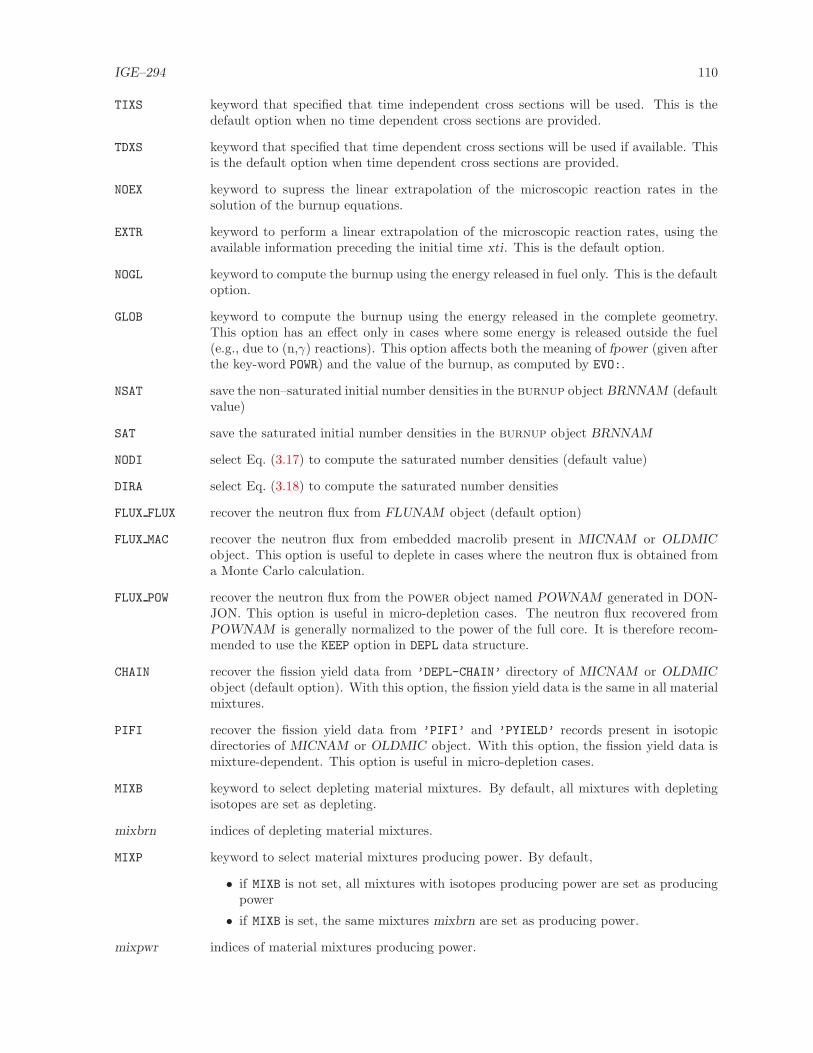
IGE–294 110

TIXS keyword that specified that time independent cross sections will be used. This is thedefault option when no time dependent cross sections are provided.

TDXS keyword that specified that time dependent cross sections will be used if available. Thisis the default option when time dependent cross sections are provided.

NOEX keyword to supress the linear extrapolation of the microscopic reaction rates in thesolution of the burnup equations.

EXTR keyword to perform a linear extrapolation of the microscopic reaction rates, using theavailable information preceding the initial time xti. This is the default option.

NOGL keyword to compute the burnup using the energy released in fuel only. This is the defaultoption.

GLOB keyword to compute the burnup using the energy released in the complete geometry.This option has an effect only in cases where some energy is released outside the fuel(e.g., due to (n,γ) reactions). This option affects both the meaning of fpower (given afterthe key-word POWR) and the value of the burnup, as computed by EVO:.

NSAT save the non–saturated initial number densities in the burnup object BRNNAM (defaultvalue)

SAT save the saturated initial number densities in the burnup object BRNNAM

NODI select Eq. (3.17) to compute the saturated number densities (default value)

DIRA select Eq. (3.18) to compute the saturated number densities

FLUX FLUX recover the neutron flux from FLUNAM object (default option)

FLUX MAC recover the neutron flux from embedded macrolib present in MICNAM or OLDMICobject. This option is useful to deplete in cases where the neutron flux is obtained froma Monte Carlo calculation.

FLUX POW recover the neutron flux from the power object named POWNAM generated in DON-JON. This option is useful in micro-depletion cases. The neutron flux recovered fromPOWNAM is generally normalized to the power of the full core. It is therefore recom-mended to use the KEEP option in DEPL data structure.

CHAIN recover the fission yield data from ’DEPL-CHAIN’ directory of MICNAM or OLDMICobject (default option). With this option, the fission yield data is the same in all materialmixtures.

PIFI recover the fission yield data from ’PIFI’ and ’PYIELD’ records present in isotopicdirectories of MICNAM or OLDMIC object. With this option, the fission yield data ismixture-dependent. This option is useful in micro-depletion cases.

MIXB keyword to select depleting material mixtures. By default, all mixtures with depletingisotopes are set as depleting.

mixbrn indices of depleting material mixtures.

MIXP keyword to select material mixtures producing power. By default,

• if MIXB is not set, all mixtures with isotopes producing power are set as producingpower

• if MIXB is set, the same mixtures mixbrn are set as producing power.

mixpwr indices of material mixtures producing power.

IGE–294 111

3.10.2 Power normalization in EVO:

Flux-induced depletion is dependent of the flux or power normalization factor given after key-wordsFLUX, POWR or W/CC. The depletion steps, given after key-words SAVE, DEPL or SET, are set in time units.Traditionally, the power normalization factor is given in MW tonne−1 and the depletion steps are givenin MWday tonne−1. However, a confusion appear in cases where some energy is released outside the fuel(e.g., due to (n,γ) reactions).

The accepted rule and default option in EVO: is to compute the burnup steps in units ofMWday tonne−1

by considering only the energy released in fuel (and only the initial mass of the heavy elements presentin fuel). However, it is also recommended to provide a normalization power taking into account thetotal energy released in the global geometry. The GLOB option can be use to change this rule and to usethe energy released in the complete geometry to compute the burnup. However, this is not a commonpractice, as it implies a non-usual definition of the burnup. A more acceptable solution consists in settingthe normalization power in power per unit volume of the complete geometry using the key-word W/CC.The value of apower can be computed from the linear power flin (expressed in Mev s−1 cm−1) using:

apower =flin 1.60207× 10−13

Vassmb(3.24)

where Vassmb is the 2–D lumped volume of the assembly expressed in cm2.

The corresponding normalization factor fburnup in MW tonne−1 is given as

fburnup =apower

Dg Fpower(3.25)

where Dg is the mass of heavy elements per unit volume of the complete geometry (g cm−3) and Fpower

is the ratio of the energy released in the complete geometry over the energy released in fuel. Numericalvalues of Dg and fpower are computed by EVO: when the parameter iprint is greater or equal to 2. Theburnup B corresponding to an elapsed time ∆t is therefore given as

B = fburnup ∆t (3.26)

where B is expressed in MWday tonne−1 and ∆t is expressed in day .

The unit of the reaction rates depends on the normalization applied to the flux. This normalizationtakes place after the flux calculation, using the EVO: module. Here is an example:

INTEGER istep := 1 ;

REAL Tend := 0.0 ;

REAL Fuelpwr := 38.4 ; ! expressed in MW/tonne

BURN MICROLIB := EVO: MICROLIB FLUX TRACKN ::

EDIT 0

SAVE <<Tend>> DAY POWR <<Fuelpwr>>

;

where BURN is the burnup object, MICROLIB is the Microlib used to compute the flux, FLUX is the flux objectand TRACKN is the tracking object used to compute the flux. After this call, the record ’FLUX-NORM’ inBURN contains a unique real number, equal to the flux normalization factor. If MICROLIB is obtained usingthe LIB: module, the DEPL keyword with following data must be set (see Section 3.2.1). Unfortunately,the normalization factor is kept aside and is not applied to the flux present in object FLUX. In fact, onlythe advanced post-processing modules COMPO: (see Section 3.14) and SAP: (see Section 3.19) are makinguse of this normalization factor.

IGE–294 112

3.11 The SPH: module

The superhomogeneisation (SPH) equivalence technique is based on the calculation of a set of equiv-alence factors µm,k,m ∈ Cm and k ∈ Mk, where Cm and Mk is a macro region and a coarse energygroup of a full-core or macro calculation (see Sect. 4.4 of Ref. 1). These equivalence factors are computedin such a way that a macro calculation made over Cm and Mk with a simplified transport operator leadsto the same leakage and reaction rates as a reference calculation performed without homogenization andwith a fine group discretization.

The SPH correction is applied differently, depending on the type of macro-calculation:

• In the case where the macro-calculation is done with the diffusion theory, neutron balance is satisfiedif the SPH correction is applied as follows:

∇ · Jg(r) + µgΣg(r)φg(r)

µg=

χg

keff

G∑

h=1

µhνΣf,h(r)φh(r)

µh+

G∑

h=1

µhΣs0,g←h(r)φh(r)

µh(3.27)

and

Jg(r) = −µgDg(r)∇φg(r)

µg. (3.28)

In conclusion:

– Diffusion coefficients and all P0 cross sections (including the total cross section NTOT0) mustbe multiplied by µg.

– Scattering matrix terms Σs0,g←h(r) must be multiplied by µh.

– Fluxes (such as NWT0 and FLUX-INTG) must be divided by µg.

• In the case where the macro-calculation is done with the simplified Pn method, the neutron balanceis satisfied if the SPH correction is applied on even parity equations as follows:[90]

µgΣ0,g(r)φ0,g(r)

µg+∇·φ1,g(r) =

χg

keff

G∑

h=1

µhνΣf,h(r)φ0,h(r)

µh+

G∑

h=1

µhΣs0,g←h(r)φ0,h(r)

µh(3.29)

2ℓ

4ℓ+ 1∇·φ2ℓ−1,g(r)+µgΣ0,g(r)

φ2ℓ,g(r)

µg+2ℓ+ 1

4ℓ+ 1∇·φ2ℓ+1,g(r) =

G∑

h=1

µhΣs2ℓ,g←h(r)φ2ℓ,h(r)

µh(3.30)

and on odd-parity equations as follows:

2ℓ+ 1

4ℓ+ 3∇φ2ℓ,g(r)

µg+Σ1,g(r)

µgφ2ℓ+1,g(r)+

2ℓ+ 2

4ℓ+ 3∇φ2ℓ+2,g(r)

µg=

G∑

h=1

Σs2ℓ+1,g←h(r)

µgφ2ℓ+1,h(r)(3.31)

where ℓ ≥ 1.

In conclusion:

– All P0 cross sections (including the total cross section NTOT0 in the even-parity equations)must be multiplied by µg.

– The total cross section NTOT1 in the odd-parity equations must be divided by µg.

– Scattering matrix terms Σsℓ,g←h(r) with ℓ even must be multiplied by µh.

– Scattering matrix terms Σsℓ,g←h(r) with ℓ odd must be divided by µg.

– Even parity fluxes (such as NWT0 and FLUX-INTG) must be divided by µg.

– Odd parity fluxes (such as NWT1 and FLUX-INTG-P1) are not modified.

IGE–294 113

• In the case where the macro-calculation is done in transport theory, but not with a Pn–type method,the macroscopic total cross section is not modified, and the even-odd corrections consistent withthe simplified Pn method are reported to the macroscopic within-group scattering cross sections.They are now corrected as[91]

Σs2ℓ,g←g(r) = µgΣs2ℓ,g←g(r) + (1− µg)Σ0,g(r) (3.32)

and

Σs2ℓ+1,g←g(r) =Σs2ℓ+1,g←g(r)

µg+

(

1−1

µg

)

Σ1,g(r) (3.33)

where ℓ ≥ 0.

Other cross sections and scattering matrix terms are corrected the same way as for the simplifiedPn method.

3.11.1 Data input for module SPH:

The SPH:module perform a SPH equivalence calculation using information recovered in a macrolib andapply SPH factors to the corresponding edition (L EDIT),microlib (L LIBRARY),macrolib (L MACROLIB)or saphyb (L SAPHYB) object. This module is also useful to extract a corrected or non-correctedmicrolib

or macrolib from the first RHS object. The calling specification is:

Table 51: Structure (SPH:)

EDINEW | LIBNEW | MACNEW | SAPNEW | CPONEW | EDINAM | LIBNAM | MACNAM| SAPNAM | CPONAM := SPH: EDINAM | LIBNAM | MACNAM | SAPNAM | CPONAM [ TRKNAM [ TRKFIL ] ] [ FLUNAM ]:: (descsph)

where

EDINEW character*12 name of the new edition data structure containing SPH-correctedinformation (see Section 3.9). In this case, an existing edition data structure mustappear on the RHS.

LIBNEW character*12 name of the new microlib data structure containing SPH-correctedinformation (see Section 3.2). In this case, an existing edition, microlib or multi-compo data structure must appear on the RHS.

MACNEW character*12 name of the new macrolib data structure containing SPH-correctedinformation (see Section 3.1).

SAPNEW character*12 name of the new saphyb data structure containing SPH information(see Section 3.19). In this case, data structure SAPNAM must appear on the RHS.

CPONEW character*12 name of the new multicompo data structure containing SPH-correctedinformation (see Section 3.14). In this case, data structure CPONAM must appear onthe RHS.

IGE–294 114

EDINAM character*12 name of the existing edition data structure where the edition infor-mation is recovered (see Section 3.9).

LIBNAM character*12 name of the existing microlib data structure where the edition infor-mation is recovered (see Section 3.2).

MACNAM character*12 name of the existing macrolib data structure where the edition infor-mation is recovered (see Section 3.1).

SAPNAM character*12 name of the existing saphyb data structure where the edition informa-tion is recovered (see Section 3.19).

CPONAM character*12 name of the existing multicompo data structure where the editioninformation is recovered (see Section 3.14).

TRKNAM character*12 name of the existing tracking data structure containing the trackingof the macro-geometry (see Section 3.4). This object is compulsory only if a macro-calculation is to be performed by module SPH:.

TRKFIL character*12 name of the existing sequential binary tracking file used to store thetracks lengths of the macro-geometry. This file is given if and only if it was requiredin the previous tracking module call (see Section 3.4).

FLUNAM character*12 name of an initialization flux used to start SPH iterations (see Sec-tion 3.8). By default, a flat estimate of the flux is used.

(descsph) structure containing the input data to this module (see Section 3.11.2).

Note: Saphyb files generated by APOLLO2 don’t have a signature. If such a Saphyb is given as inputto module SPH:, a signature must be included before using it. The following instruction can do the job:

Saphyb := UTL: Saphyb :: CREA SIGNATURE 3 = ’L_SA’ ’PHYB’ ’ ’ ;

3.11.2 Specification for the type of equivalence calculation

This structure is used to specify the type of equivalence calculation where the flux and the condensedand/or homogenized cross sections are corrected by SPH factors, in such a way as to respect a specifiedtransport-transport or transport-diffusion equivalence criteria.[68–70] This structure is defined as:

Table 52: Structure (descsph)

[ EDIT iprint ][[ STEP UP NOMDIR | AT index ]][ IDEM | MACRO | MICRO ][ OFF | SPRD [ nmerge ngcond (sph(i), i=1, nmerge×ngcond) ] | HOMO | ALBS ][ PN | SN [ BELL ] ][ STD | SELE ALB | SELE FD | SELE MWG | SELE EDF | ASYM mixs ] [ ARM ][ ITER [ maxout ] [ epsout ] ][ MAXNB maxnb ][ EQUI TEXT4 [ LOCNAM TEXT80 ] ][ LEAK b2 ]

where

IGE–294 115


iprint index used to control the printing of this module. The iprint parameter is importantfor adjusting the amount of data that is printed by this calculation step.

STEP keyword used to set a specific elementary calculation from the first RHS.

UP keyword used to select an elementary calculation located in a subdirectory of EDINAMor CPONAM . By default,

• the sub-directory name stored in record ’LAST-EDIT’ is selected if EDINAM isdefined at RHS.

• the sub-directory ’default’ is selected if CPONAM is defined at RHS.

NOMDIR name of an existing sub-directory of EDINAM or CPONAM .

AT keyword used to select the index–th elementary calculation in SAPNAM or CPONAM .

index index of the elementary calculation.

IDEM keyword to force the production of a LCM object of the same type as the RHS.

MACRO keyword to force the production of a macrolib at LHS.

MICRO keyword to force the production of a microlib at LHS.

OFF keyword to specify the SPH factors are all set to 1.0, meaning no correction. Thiskeyword is useful to get rid of a SPH correction which have been set previously. Bydefault, the PN or SN option is activated.

SPRD keyword to specify that the SPH factors are read from input (if nmerge, ngcond andsph are set) or recovered from a RHS object (otherwise).

nmerge number of regions.

ngcond number of energy groups.

sph(i) initial value of each SPH factor in each mixture (inner loop) and each group (outerloop).

HOMO keyword to specify that the SPH factors are uniform over the complete macro-geometry.This option is generally used with a complete homogenization of the reference geom-etry, obtained using option MERG COMP. In this case the neutron flux (transport ordiffusion) will be uniform, which allows the SPH factors to be obtained (one permacro-group) using a non-iterative strategy. For a given macro-group the SPH factorwill be equal to the ratio between the average flux of the region and the surface fluxif the SELE option is used otherwise the SPH factor are all set equal to 1.0 (no correc-tion). The SELE option allows an SPH factor equal to the inverse of the discontinuityfactor to be calculated.

ALBS keyword to specify that the albedo of the geometry are to be taken into accountin the complete homogenization process. Thus the MERG and COMP options must bespecified. The SPH factors are obtained using a transport-transport equivalence basedon a calculation using the collision probabilities. This option requires a geometrywith VOID (see Section 3.3.2) external boundary conditions to be closed using ALBS inmodules ASM: (see Section 3.7.1).[69]

PN keyword to activate a calculation of heterogeneous SPH factors based on a converg-ing series of macro-calculations with the correction strategy of Eqs. (3.27) to (3.31).This is the default option if the macro-calculation is of diffusion, PN or SPN type.A normalization condition must be set if the macro-geometry has no boundary leak-age (fundamental mode condition). If boundary leakage is present, no normalizationcondition is used but the SPH iterations are difficult to converge in this case.

IGE–294 116

SN keyword to activate a calculation of heterogeneous SPH factors based on a converg-ing series of macro-calculations with the correction strategy of Eqs. (3.32) and (3.33).This is the default option if the macro-calculation is of PIJ, IC, SN or MOC type.A normalization condition must be set if the macro-geometry has no boundary leak-age (fundamental mode condition). If boundary leakage is present, no normalizationcondition is used but the SPH iterations are difficult to converge in this case.

BELL keyword to activate the Bell procedure to accelerate the convergence of the SPH factors.This feature is currently available with macro-calculations of PIJ type.[71]

STD keyword to specify the use of flux-volume normalization for the SPH factors (defaultoption). In each macro-group, the macro-fluxes in macro regions i are normalizedusing

φi = φiφref

φmc

where φref is the averaged volumic flux of the reference calculation and φmc is theaveraged volumic flux of the macro-calculation. Using this definition, the averagedSPH factor is equal to one.

SELE ALB keyword to specify the use of Selengut normalization for the SPH factors. It is neces-sary to know the averaged surfacic flux of the reference calculation. Two possibilitiesexist:

• We use collision probabilities. We define the reference geometry with VOID ex-ternal boundary conditions (see Section 3.3.2) and to close the region for thecollision probability calculations using the ALBS option (see Section 3.7.1).

• We perform a flux calculation with the current iteration method in Eurydice.This option is only available if a SYBILT: tracking is used and if keyword ARM isset in module ASM: (see Section 3.7.1).

SELE FD keyword to specify the use of Selengut normalization for the SPH factors. It is neces-sary to know the averaged surfacic flux of the reference calculation. This value can beobtained by defining a small region near boundary in the reference geometry and byusing the ADF FD B data structure in Section 3.9.1.

In each macro-group, the macro-fluxes in macro regions i are normalized using

φi = φiφgapref

φmc

where φgapref is the averaged surfacic flux of the reference calculation. Using this defini-

tion, the averaged SPH factor is equal to

µ =φref

φgapref

.

SELE MWG keyword to specify the use of Selengut macro calculation water gap normalization forthe SPH factors.[72] It is necessary to know the averaged surfacic flux of the referenceand that of the macro calculations. This reference value can be obtained by defining asmall region near boundary in the reference geometry and by using the ADF FD B datastructure in Section 3.9.1.


φi = φiφgapref

φsurfmc

where φgapref is the averaged surfacic flux of the reference calculation and φsurf

mc is theaveraged surfacic flux of the macro calculation. Using this definition, the averagedSPH factor is equal to

µ =φref φ

surfmc

φmc φgapref

.

IGE–294 117

SELE EDF keyword to specify the use of generalized Selengut normalization for the SPH factors.[73]

It is necessary to know the averaged surfacic flux and the averaged volumic flux in arow of cells of the reference calculation. The surfacic flux is obtained as with theSELE option. The value of the volumic flux in a row of cells is computed using indexinformation from the ADF FD H data structure in Section 3.9.1.


φi = φiφref φ

gapref

φmc φrowref

where φgapref is the averaged surfacic flux of the reference calculation and φrow

ref is theaveraged volumic flux in a row of cells of the reference calculation. Using this definition,the averaged SPH factor is equal to

µ =φrowref

φgapref

.

ASYM keyword to specify the use of asymptotic normalization of the SPH factors. The SPHfactors in homogenized mixture mixs are set to one in all macro-energy groups.

mixs index of the homogenized mixture where asymptotic normalization is performed.

ARM keyword to activate a solution technique other than the collision probability method.Used with the Eurydice solution technique within SYBILT: to activate the currentiteration method.

ITER keyword to specify the main convergence parameters used to control SPH iterations.

maxout user-defined maximum number of SPH iterations (default value: 200).

epsout user-defined convergence criterion (default value: 1.0× 10−4).

MAXNB keyword to specify an auxiliary convergence parameter used to control SPH iterations.

maxnb acceptable number of SPH iterations with an increase in convergence error beforeaborting (default value: 10).

EQUI keyword used to select an existing set of SPH factors in SAPNAM or to store a newset of SPH factors in SAPNEW or SAPNAM .

TEXT4 character*4 user-defined keyword of a set of SPH factors. This keyword is related tovariable parkey , as defined in Sect. 3.19.1 for a local variable.

LOCNAM keyword used to define a character*80 name for the set of SPH factors, if this set iscreated. By default, TEXT80 is taken equal to TEXT4 .

TEXT80 character*80 user-defined name associated to keyword TEXT4 . This name is relatedto variable parnam, as defined in Sect. 3.19.1 for a local variable.

LEAK keyword used to introduce leakage in the embedded macrolib. This option shouldonly be used for non-regression tests.

b2 the imposed buckling corresponding to the leakage.

IGE–294 118

3.12 The CFC: module

The CFC: module is used to generate a Feedback Model database required for a full core calculationin DONJON.[88] The general specifications of this module are:

Table 53: Structure (CFC:)

CFCNAM := CFC: [ CFCNAM ](CPONAM(i), i=1,28) :: (desccfc)

where

CFCNAM character*12 name of the fbmxsdb data structure containing the Feedback Modelreactor database. The reactor database can be updated if CFCNAM appears on theRHS.

CPONAM character*12 name of read only cpo data structures. There are 28 different cpo

data structures required here each containing respectively

1. the reactor reference cross section.

2. cell cross section for the first fuel temperature.

3. cell cross section for the second fuel temperature.

4. cell cross section for the first coolant temperature.

5. cell cross section for the second coolant temperature.

6. cell cross section for the first moderator temperature.

7. cell cross section for the second moderator temperature.

8. cell cross section for the first coolant density.

9. cell cross section for the second coolant density.

10. cell cross section for the first moderator density.

11. cell cross section for the second moderator density.

12. cell cross section for a different concentration of boron.

13. cell cross section for a different moderator purity.

14. cell cross section for a different concentration of xenon.

15. cell cross section for a different concentration of samarium.

16. cell cross section for a different concentration of neptunium.

17. cell cross section for the spectral mixed effect fuel/coolant density.

18. cell cross section for the spectral mixed effect coolant density/temperature.

19. cell cross section for low power history.

20. cell cross section for intermediate power history.

21. cell cross section for high power history.

22. reactor reference moderator cross section.

23. moderator cross section for the first moderator temperature.

24. moderator cross section for the second moderator temperature.

25. moderator cross section for the first moderator density.

26. moderator cross section for the second moderator density.

IGE–294 119

27. moderator cross section for a different concentration of boron.

28. moderator cross section for a different moderator purity.

(desccfc) structure containing the input data to this module (see Section 3.12.1).

3.12.1 Data input for module CFC:

Table 54: Structure (desccfc)

[ EDIT iprint ][ INFOR TITLE ][ DNAME RNANE ][ PWR powerref powerup powerint powerdown ][ TCOOL tcoolref tcoolup tcooldown ][ TMODE tmoderef tmodeup tmodedown ][ TFUEL tfuelref tfuelup tfueldown ][ RHOC denscool][ RHOM densmode][ XIR purityref puritydown ]

where


iprint index used to control the printing of the module.

INFOR keyword which allows to set the title.

TITLE character*72 title associated to the reactor database generated.

DNAME keyword to set a specific database name in the data structure.

RNAME character*12 name of the feedback database.

PWR keyword to specify power used for evolution for power history.

powerref power value for regular power history (CPONAM default).

powerup power value for high power history (CPONAM 21).

powerint power value for intermediate power history (CPONAM 20).

powerdown power value for low power history (CPONAM 19).

TCOOL keyword to specify coolant temperature used for regular evolution and perturbed cases.

tcoolref normal coolant temperature (CPONAM default).

tcoolup high coolant temperature (CPONAM 4).

tcooldown low coolant temperature (CPONAM 5).

TMODE keyword to specify moderator temperature used for regular evolution and perturbedcases.

IGE–294 120

tmoderef normal moderator temperature (CPONAM default).

tmodeup high moderator temperature (CPONAM 6 and 23).

tmodedown low moderator temperature (CPONAM 7 and 24).

TFUEL keyword to specify fuel temperature used for regular evolution and perturbed cases.

tfuelref normal fuel temperature (CPONAM default).

tfuelup high fuel temperature (CPONAM 2).

tfueldown low fuel temperature (CPONAM 3).

RHOC keyword to specify coolant density used for regular evolution.

denscool normal coolant density (CPONAM default).

RHOM keyword to specify moderator density used for regular evolution.

densmode normal moderator density (CPONAM default).

XIR keyword to specify water purity (D2O content) used for regular evolution and per-turbed cases.

purityref normal moderator purity (fraction of D2O in water) (CPONAM default).

puritydown perturbed moderator purity (fraction of D2O in water) (CPONAM 13 and 28).

Note: Other perturbed values are recovered directly from the concentrations and isotope densitiesstored in the different CPONAM .

IGE–294 121

3.13 The INFO: module

The INFO: module is mainly used to compute the number densities for selected isotopes at specificlocal conditions. The module can also be used to compute the water density ρ(T, P ) according to theassumed temperature T and purity P . In that case, the compound water density for a mix of light andheavy water is

ρ(T, P ) =100 ρH2O(T ) ρD2O(T )

P ρH2O(T ) + (1− P ) ρD2O(T ).

Temperature tabulations for ρH2O(T ) and ρD2O(T ) are the same as those of the WIMS–AECL code.

The calling specifications are:

Table 55: Structure (INFO:)

INFO: :: (descinfo)

where

(descinfo) structure containing the input data to this module (see Section 3.13.1).

3.13.1 Data input for module INFO:

Table 56: Structure (info)

[ EDIT iprint ][ LIB: DRAGON | MATXS | MATXS2 | WIMSD4 | WIMS | WIMSAECL | NDAS | APLIB2 | APLIB1

FIL: NAMEFIL ][ TMP: temp K | C ][ PUR: purity WGT% | ATM% ][ CALC DENS WATER >>dens<< ][ ENR: enrichment WGT% | ATM% ][[ ISO: nbiso (ISONAM(i), i=1,nbiso) GET MASS (>>mass(i)<<, i=1,nbiso) | CALC WGT%

D2O >>nh1<< >>hd2<< >>no16<< |UO2 >>nu5<< >>hu8<< >>no16<< |THO2 >>nth2<< >>nu3<< >>no16<< ]]

where


iprint index used to control the printing of the module. The amount of output produced bythis tracking module will vary substantially depending on the print level specified.

LIB: keyword to specify the type of library from which the isotopic mass ratio is to be read.

IGE–294 122

DRAGON keyword to specify that the isotopic depletion chain or the microscopic cross sectionsare in the DRAGLIB format.

MATXS keyword to specify that the microscopic cross sections are in the MATXS format ofNJOY-II and NJOY-89 (no depletion data available for libraries using this format).

MATXS2 keyword to specify that the microscopic cross sections are in the MATXS format ofNJOY-91 (no depletion data available for libraries using this format).

WIMSD4 keyword to specify that the isotopic depletion chain and the microscopic cross sectionsare in the WIMSD4 format.

WIMS keyword to specify that the isotopic depletion chain and the microscopic cross sectionsare in the WIMS-AECL format.

WIMSAECL keyword to specify that the isotopic depletion chain and the microscopic cross sectionsare in the WIMS-AECL format.

NDAS keyword to specify that the isotopic depletion chain and the microscopic cross sectionsare in the NDAS format, as used in recent versions of WIMS-AECL.

APLIB1 keyword to specify that the microscopic cross sections are in the APOLLO-1 format.

APLIB2 keyword to specify that the microscopic cross sections are in the APOLLO-2 format.

FIL: keyword to specify the name of the file where is stored the mass ratio data.

NAMEFIL character*8 name of the library where the mass ratio are stored.

TMP: keyword to specify the isotopic temperature.

temp temperature given in Kelvin (K) or Celsius (C).

PUR: keyword to specify the water purity, that is fraction of heavy water in a mix of heavyand light water.

purity water purity in weight percent (WGT%) or atomic percent (ATM%).

ENR: keyword to specify the fuel enrichment.

enrichment fuel enrichment in weight percent (WGT%) or atomic percent (ATM%).

ISO: keyword to specify an isotope list. This list will be used either for getting mass valuesof isotopes or for computing number densities.

nbiso number of isotopic names used for a calculation (limited to nbiso≤ 3).

ISONAM character*12 name of an isotope.

GET MASS keyword to recover the mass values as written in the library. It returns the mass valueof each isotope in the output parameter mass.

CALC keyword to ask the module to compute some parametric values. It returns one valuein the output parameter dens.

DENS WATER set of keywords to recover the water density as a function of its temperature and purity.This option requires the setting of temperature and purity, and it does not affect anygiven list of isotope names.

WGT% D2O keywords to recover 3 number densities for a compound mixture of heavy and lightwater. The isotope list is assumed to contain 1H, 2D and 2O. Temperature and purityare supposed to be available. It returns concentration of these isotopes in the outputparameters nh1 , nd2 and no16 .

IGE–294 123

WGT% UO2 keywords to recover 3 number densities for a compound mixture of Uranium oxide.The isotope list is assumed to contain 235U, 238U and 16O. The 235U enrichment issupposed to be available. Note that the number densities will sum to 100. It returnsconcentration of these isotopes in the output parameters nu5 , nu8 and no16 .

WGT% THO2 keywords to recover 3 number densities for a compound mixture of Thorium/Uraniumoxide. The isotope list is assumed to contain 232Th, 233U and 16O. The 233U enrichmentis supposed to be available. Note that the number densities will sum to 100. It returnsconcentration of these isotopes in the output parameters nth2 , nu3 and no16 .

The INFO: module works the following way. For a given isotope list, the mass is extracted fromthe library or a calculation process is expected. Once this calculation is has been performed, it ispossible to list other isotopes and ask for further calculations. Finally note that the number of outputparameters, denoted by >>param<<, are recovered as CLE-2000 variables in (descinfo). The numberof these parameters must be equal to the number of isotopes names given, plus the water density whena command CALC DENS WATER is issued.

IGE–294 124

3.14 The COMPO: module

This component of the lattice code is dedicated to the constitution of the reactor database intended tostore all the nuclear data, produced in the lattice code, that is useful in reactor calculations including fuelmanagement and space-time kinetics. Multigroup lattice calculations are too expensive to be executeddynamically from the driver of the global reactor calculation. A more feasible approach is to create areactor database where a finite number of lattice calculation results are tabulated against selected globaland/or local parameters chosen so as to represent expected operating conditions of the reactor.

The COMPO: module is used to create and construct a multicompo object. This object is gener-ally persistent and used to collect information gathered from many DRAGON elementary calculationsperformed under various conditions.

For each elementary calculation, the results are recovered from the output of the EDI: module andstored in a list of homogenized mixture directories. The EDI: module is responsible for performingcondensation in energy, homogenization in space of the microscopic cross sections and constitution ofmacroscopic sets for collecting together many isotopes. All the elementary calculations gathered in asingle multicompo object are characterized by the same number of homogenized mixtures and by aspecific output energy-group structure.

(geometry object)

(microlib object)

‘SIGNATURE’

namdir

‘STATE-VECTOR’

‘COMMENT’

‘GLOBAL’

‘LOCAL’

‘MIXTURES’

‘GEOMETRIES’

‘TREE’

‘CALCULATIONS’

‘DEPL-CHAIN’

Figure 20: Organization of a multicompo object.

Each elementary calculation is characterized by a tuple of global and/or local parameters Globalparameters are characteristics of the complete lattice, while local parameters are characteristics of eachhomogenized mixture. These parameters are of different types, depending on the nature of the studyunder consideration: type of assembly, power, temperature in a mixture, concentration of an isotope,time, burnup or exposure rate in a depletion calculation, etc. Each step of a depletion calculationrepresents an elementay calculation. The multicompo object is often presented as a multi-parameterreactor database.

Parameter nb. 1

Parameter nb. 2

Parameter nb. 3

(root)

(leafs)

Figure 21: Parameter tree in a multicompo object

The multicompo object is organized as shown in Figure 20. The root of the object contains table–of–content information for global and local parameters and two lists of directories. Each component of the

IGE–294 125

first list (’MIXTURES’) contains the directory ’TREE’ (the parameter tree) and the list (’CALCULATIONS’)made of microlib objects. Each component of the second list (’GEOMETRIES’) contains the homogenizedgeometry of an elementary calculation.

The localization of an elementary calculation is done using a tuple of global and/or local parameters.The elementary calculation indices are stored in a tree with the number of levels equal to the number ofglobal and local parameters. An example of a tree with three parameters is shown in Figure 21. Eachnode of this tree is associated with the index of the corresponding parameter and with the reference tothe daughter nodes if they exist. The number if leafs is equal to the number of nodes for the last (third)parameter and is equal to the number of elementary calculations stored in the multicompo object. Theindex of each elementary calculation is therefore an attribute of each leaf.

In each homogenized mixture component, the COMPO: module recover cross sections for a number ofparticularized isotopes and of a single macroscopic set, a collection of the remaining isotopic cross sectionsweighted by isotopic number densities. Other information is also recovered: multigroup neutron fluxes,isotopic number densities, fission spectrum, delayed neutron data, etc.

A different specification of the COMPO: function call is used for creation and construction of themulticompo object.

• The first specification is used to initialize the multicompo data structure and to set the choice ofglobal and local parameters.

• A modification call to the COMPO: function is performed after each elementary calculation in orderto recover output information processed by EDI: (condensed and homogenized cross sections) andEVO: (burnup dependant values). Global and local parameters can optionnally be recovered frommicrolib objects.

• Another modification call to the COMPO: function is used to catenate a read-only multicompo

object into a master multicompo object.


Table 57: Structure (COMPO:)

CPONAM := COMPO: [ CPONAM ] :: (compo data1)| CPONAM := COMPO: CPONAM EDINAM [ EDINA2 ] [ BRNNAM ] [ HMIC1 [ HMIC2 ] ]

:: (compo data2)| CPONAM := COMPO: CPONAM CPORHS :: (compo data3)| COMPO: CPONAM :: (compo data4)

where

CPONAM character*12 name of the lcm object containing the master multicompo data struc-ture.

EDINAM character*12 name of the lcm object (type L EDIT) containing the edition data struc-ture corresponding to an elementary calculation. This edition data structure is contain-ing homogenized and condensed cross-section information. The edition data producedby the last call to the EDI: module is used.

EDINA2 character*12 name of an optional lcm object (type L EDIT) containing the edition

data structure corresponding to an elementary calculation. This edition data structureis containing group form factor information. The edition data produced by the last callto the EDI: module is used.

BRNNAM character*12 name of the lcm object (type L BURNUP) containing the burnup datastructure.

IGE–294 126

HMIC1 character*12 name of a microlib (type L LIBRARY) containing global parameter infor-mation.


CPORHS character*12 name of the read-only multicompo data structure. This data structureis concatenated to CPONAM using the compo data3 data structure, as presented inSection 3.14.3. CPORHS must be defined with the same number of energy groups andthe same number of homogeneous regions as CPONAM . Moreover, all the global andlocal parameters of CPORHS must be defined in CPONAM . CPONAM may be definedwith global parameters not defined in CPORHS.

compo data1 input data structure containing initialization information (see Section 3.14.1).

compo data2 input data structure containing information related to the recovery of an elementarycalculation (see Section 3.14.2).

compo data3 input data structure containing information related to the catenation of a read-onlymulticompo (see Section 3.14.3).

compo data4 input data structure containing information related to the display of a read-only mul-

ticompo (see Section 3.14.4).

3.14.1 Initialization data input for module COMPO:

Table 58: Structure (compo data1)

[ EDIT iprint ][[ [ STEP UP NAMDIR ][ MAXCAL maxcal ][ COMM [[ HCOM ]] ENDC ][[ PARA PARKEY TEMP HMIC imix | CONC HISO1 HMIC imix | IRRA | FLUB |POWR | MASL | FLUX | TIME | VALU REAL | CHAR | INTE

]][[ LOCA PARKEY TEMP | CONC HISO2 | IRRA | FLUB | FLUG | POWR | MASL | FLUX

]][ ISOT nisp (HISOP(i),i=1,nisp) ][ GFF ]INIT ]];

where

EDIT keyword used to set iprint.

iprint index used to control the printing in module COMPO:. =0 for no print; =1 for minimumprinting (default value).

STEP keyword used to create the database from a sub-directory named NAMDIR. Thiscapability make possible the creation of a single object with many independent mul-ticompo structures in it. By default, the database is created on directory ’default’.

IGE–294 127

UP keyword used to move up towards a sub-directory of CPONAM .

NAMDIR create the multicompo structure in the sub-directory named NAMDIR.

MAXCAL keyword used to set maxcal.

maxcal maximum number of elementary calculations to be stored in the multicompo. max-cal= 10 by default. This maximum size is automatically increased when the numberof elementary calculations exceeds the current value of maxcal.

COMM keyword used to input a general comment for the multicompo.

HCOM character*80 user-defined comment.

ENDC end–of–HCOM keyword.

PARA keyword used to define a single global parameter.

LOCA keyword used to define a single local parameter.

PARKEY character*12 user-defined keyword associated to a global or local parameter.

HMIC character*12 name of the microlib (type L LIBRARY) associated to a global parame-ter. The corresponding microlib will be required on RHS of the COMPO: call describedin Sect. 3.14.2.

imix index of the mixture associated to a global parameter. This mixture is located inmicrolib named HMIC .

HISO1 character*8 alias name of the isotope associated to a global parameter. This isotopeis located in microlib data structure named HMIC .

HISO2 character*8 alias name of the isotope associated to a local parameter. This isotopeis located in the microlib directory of the edition data structure named EDINAM .

TEMP keyword used to define a temperature (in Kelvin) as global or local parameter.

CONC keyword used to define a number density as global or local parameter.

IRRA keyword used to define a burnup (in MWday/Tonne) as global or local parameter.

FLUB keyword used to define a fuel-only exposure rate (in n/kb) as global or local parameter.The exposure rate is recovered from the BRNNAM LCM object.

FLUG keyword used to define an exposure rate in global homogenized mixtures (in n/kb) aslocal parameter. The exposure rate is recovered from the BRNNAM LCM object.

POWR keyword used to define the power as global or local parameter.

MASL keyword used to define the mass density of heavy isotopes as global or local parameter.

FLUX keyword used to define the volume-averaged, energy-integrated flux as global or localparameter.

TIME keyword used to define the time (in seconds) as global parameter.

VALU keyword used to define a user-defined quantity as global parameter. This keywordmust be followed by the type of parameter.

REAL keyword used to indicate that the user-defined global parameter is a floating pointvalue.

CHAR keyword used to indicate that the user-defined global parameter is a character*12

value.

IGE–294 128

INTE keyword used to indicate that the user-defined global parameter is an integer value.

ISOT keyword used to select the set of particularized isotopes. By default, all the isotopesavailable in the edition data structure EDINAM are selected.

nisp number of user-defined particularized isotopes.

HISOP character*8 names of the user-defined particularized isotopes. These names must bepresent in the edition data structure EDINAM .

GFF keyword used to enable the recovery of group form factor information from edition

data structure EDINA2 .

INIT keyword used to create the empty structure in the multicompo.

IGE–294 129

3.14.2 Modification data input for module COMPO:


[ EDIT iprint ][ ALLX ][ STEP UP NAMDIR | * ][ ORIG orig ][[ PARKEY value ]][ MACRO ] [ SET xtr S | DAY | YEAR ];

where



ALLX keyword used to register the region number of each isotope before merging. This optionis useful if the same keyword has been specified in EDI: before. This allows to performsubsequent depletion calculations, in taking into account different fuel regions in thediffusion calculation.

STEP keyword used to access the database from a sub-directory named NAMDIR instead ofaccessing it from the root of CPONAM .

UP keyword used to move up towards a sub-directory of CPONAM .

NAMDIR access the multicompo structure in the sub-directory named NAMDIR.

* use a sub-directory name identical to the directory in EDINAM where the edition datais coming from.

PARKEY character*12 keyword associated to a user-defined global parameter.

value floating-point, integer or character*12 value of a user-defined global parameter.

ORIG keyword used to define the father node in the parameter tree. By default, the indexof the previous elementary calculation is used.

orig index of the elementary calculation associated to the father node in the parametertree.

MACRO keyword used to recover cross-section information from the macrolib directory in ED-INAM . By default, the cross-section information is recovered from the microlib inEDINAM .

SET keyword used to recover the flux normalization factor already stored on BRNNAMfrom a sub-directory corresponding to a specific time.

xtr time associated with the current flux calculation. The name of the sub-directory wherethis information is stored will be given by ‘DEPL-DAT’//CNNwhere CNN is a character*4variable defined by WRITE(CNN,’(I4.4)’) INN where INN is an index associated withthe time xtr.


IGE–294 130



3.14.3 Modification (catenate) data input for module COMPO:


[ EDIT iprint ][ STEP UP NAMDIR ][ ORIG orig ][[ PARKEY value ]][ WARNING-ONLY ];

where



PARKEY character*12 keyword associated to a global parameter that is specific to CPONAM(not defined in CPORHS).

value floating-point, integer or character*12 value of a global parameter that is specific toCPONAM .



WARNING-ONLY This option is useful if an elementary calculation in CPORHS is already present inCPONAM . If this keyword is set, a warning is send and the CPONAM values arekept, otherwise the run is aborted (default).

3.14.4 Display data input for module COMPO:


[ EDIT iprint ][ STEP UP NAMDIR ][ EDIT iprint ]DB-STRUC

;

IGE–294 131

where


iprint index used to control the printing in module COMPO:. <2 for MUPLET display only(default value) and parameters values are presented at the end, ≥2 for the parametervalue display for each calculation.

DB-STRUC character*12 keyword used to display the content of the CPONAM object for theNAMDIR directory.

IGE–294 132

3.15 The TLM: module

The TLM: module has been designed to generate a Matlab m-file (in an ASCII format) that containsthe instructions for plotting the tracking lines generated by the NXT: module (EDIT -1000 option).[80] TheTLM: module is activated using the following list of commands:

Table 62: Structure (TLM:)

MFILE := TLM: MFILE TRKNAM TRKFIL :: (desctlm)

where

MFILE character*12 name of the ASCII Matlab m-file data structure that will contain theinstructions for plotting the tracking lines.

TRKNAM character*12 name of the tracking data structure that will contain region volumeand surface area vectors in addition to region identification pointers and other trackinginformation.

TRKFIL character*12 name of the sequential binary tracking file used to store the trackslengths.[89]

(desctlm) structure describing the type of graphics generated (see Section 3.15.1).

3.15.1 Data input for module TLM:

Table 63: Structure (desctlm)

[ EDIT iprint ][ NTPO nplots ](

POINTS [ NoPause ] |DIRECTIONS [ NoPause ] DIR idir [ PLAN iplan U iuv | V iuv ] |PLANP [ NoPause ] DIR idir DIST dist [ PLAN iplan ] |PLANA [ NoPause ] A a B b [ C c ] D d , iplot=1, nplots )

where


iprint index used to control the printing in this module. It must be set to 0 if no printing onthe output file is required.

NTPO keyword to specify the number of figures to draw.

nplots integer value for the number of figures to draw.

IGE–294 133

POINTS keyword to specify that the figure will illustrate the intersection points between thelines and the external faces of the geometry.

DIRECTIONS keyword to specify that the figure will illustrate the lines crossing each region as wellas the intersection points between the lines and the external faces of the geometry.

PLANP keyword to specify that the figure will illustrate the points crossing a plane normal tothe line direction.

PLANA keyword to specify that the figure will illustrate the points crossing an arbitrary surfacein 3-D or line in 2-D. The equation for the surface in 3-D is :

aX + bY + cZ = d

while the equation for the line in 2-D is :

aX + bY = d

NoPause keyword to specify that all the lines the lines must be drawn without Matlab pause.By default, there is a pause after all the points associated with an external surface andall the lines associated with a region are drawn.

DIR keyword to specify line direction to draw.

idir integer value to identify the track direction to draw. In the case where idir=0, allthe directions will be drawn. A value of idir=0 for 2-D geometry is generally accept-able. However, for 3-D geometry the number of lines generated is such that the figurebecomes a mess and it is generally more convenient to draw the lines direction perdirection.

PLAN keyword to specify which of the three planes normal to the specified direction in 3-Dwill be considered for drawing. This plane is defined by the axes U − V . Used onlyfor 3-D geometries.

iplan integer value to identify which of the three planes normal to the specified direction in3-D will be considered for drawing. the only values permitted are 0, 1, 2 or 3. Whena value of 0 is specified (default) all three planes will be drawn. Used only for 3-Dgeometries.

U keyword to specify that the all the lines in the V axis associated with a position onthe U axis will be drawn. Used only for 3-D geometries.

V keyword to specify that the all the lines in the U axis associated with a position onthe V axis will be drawn. Used only for 3-D geometries.

iuv integer value to identify the position on the U or V axis to be drawn. Used only for3-D geometries.

DIST keyword to specify the distance between the plane normal to the line direction and theorigin.

dist real or double precision value for the distance of the plane from the origin.

A keyword to specify the value of a for an arbitrary plane or line.

a real or double precision value a.

B keyword to specify the value of b for an arbitrary plane or line.

b real or double precision value b.

C keyword to specify the value of c for an arbitrary plane.

IGE–294 134

b real or double precision value c.

D keyword to specify the value of d for an arbitrary plane or line.

d real or double precision value d.

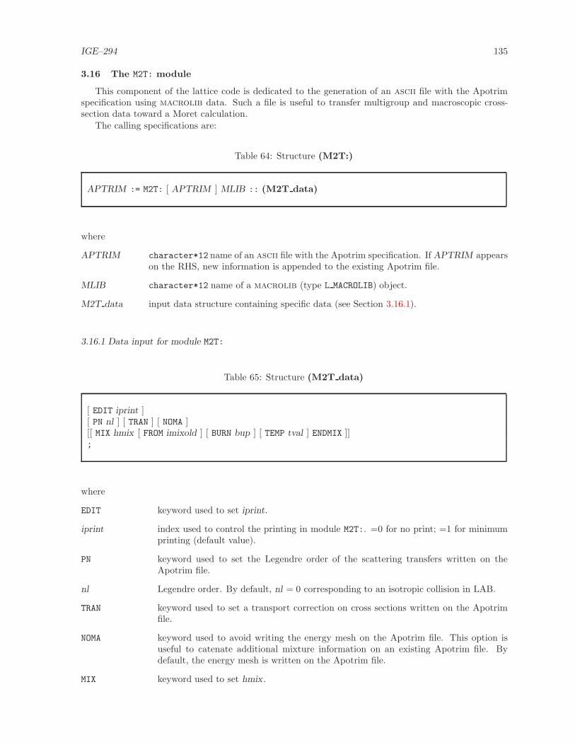
IGE–294 135

3.16 The M2T: module

This component of the lattice code is dedicated to the generation of an ascii file with the Apotrimspecification using macrolib data. Such a file is useful to transfer multigroup and macroscopic cross-section data toward a Moret calculation.


Table 64: Structure (M2T:)

APTRIM := M2T: [ APTRIM ] MLIB :: (M2T data)

where

APTRIM character*12 name of an ascii file with the Apotrim specification. If APTRIM appearson the RHS, new information is appended to the existing Apotrim file.

MLIB character*12 name of a macrolib (type L MACROLIB) object.

M2T data input data structure containing specific data (see Section 3.16.1).

3.16.1 Data input for module M2T:

Table 65: Structure (M2T data)

[ EDIT iprint ][ PN nl ] [ TRAN ] [ NOMA ][[ MIX hmix [ FROM imixold ] [ BURN bup ] [ TEMP tval ] ENDMIX ]];

where


iprint index used to control the printing in module M2T:. =0 for no print; =1 for minimumprinting (default value).

PN keyword used to set the Legendre order of the scattering transfers written on theApotrim file.

nl Legendre order. By default, nl = 0 corresponding to an isotropic collision in LAB.

TRAN keyword used to set a transport correction on cross sections written on the Apotrimfile.

NOMA keyword used to avoid writing the energy mesh on the Apotrim file. This option isuseful to catenate additional mixture information on an existing Apotrim file. Bydefault, the energy mesh is written on the Apotrim file.

MIX keyword used to set hmix.

IGE–294 136

hmix character*20 name of the mixture to be written on the Apotrim file.

BURN keyword used to set the burnup of a mixture.

bup burnup of a mixture. By default, bup = 0.0.

TEMP keyword used to set the temperature of a mixture.

tval temperature of a mixture in Celsius. By default, tval = 0.0 C.

FROM keyword used to set the index of the mixture in the macrolib object.

imixold index of the mixture that is recovered in the macrolib object. By default, imixold= 1.

ENDMIX end of specification keyword for the material mixture.

Here is an example of the creation of an Apotrim file named APOTR with a Hansen-Roach energy meshcreated from a XMAS 172-group flux calculation. The Apotrim file is created from three LCM objectsFLUX, LIBRARY2 and TRACK containing the flux, the XMAS-formatted microlib and the tracking.

LINKED_LIST TRACK LIBRARY2 FLUX MAC2 EDIT ;

SEQ_ASCII APOTR ;

...

EDIT := EDI: LIBRARY2 TRACK FLUX :: EDIT 3

* Hansen-Roach energy mesh follows

COND 12 17 21 27 33 42 50 60 66 76 84 95 123 140 155 172

MERGE MIX 1 1 1 1 1 1 2 3 3

SAVE ON ’EDITCDAT 1’ ;

MAC2 := EDIT :: STEP UP ’EDITCDAT 1’ STEP UP ’MACROLIB’ ;

APOTR := M2T: MAC2 :: EDIT 3 TRAN MIX FUEL FROM 1 ENDMIX

MIX CLAD FROM 2 ENDMIX

MIX COOLANT FROM 3 ENDMIX ;

IGE–294 137

3.17 The CHAB: module

This component of the lattice code is dedicated to the modification of cross section information in amicrolib.


Table 66: Structure (CHAB:)

MICRO1 | DRAGLIB1 := CHAB: MICRO1 | MICRO2 | DRAGLIB2 :: (CHAB data)

where

MICRO1 character*12 name of a microlib (type L LIBRARY) object that is created or modifiedby CHAB:.

DRAGLIB1 character*12 name of a draglib (type L DRAGLIB) object that is created by CHAB:.

MICRO2 character*12 name of a microlib (type L LIBRARY) object open in read-only mode.

DRAGLIB2 character*12 name of a draglib (type L DRAGLIB) object open in read-only mode.

CHAB data input data structure containing specific data (see Section 3.17.1).

3.17.1 Data input for module CHAB:

Table 67: Structure (CHAB data)

[ EDIT iprint ][[ MODI TYPSEC igm TO igp VALE [[ val ]] | CONS value | PLUS value | MULT value HISOT ]] ;

where


iprint index used to control the printing in module CHAB:. =0 for no print; =1 for minimumprinting (default value).

MODI keyword used to define a modification of a nuclear reaction belonging to a given isotope.

TYPSEC character*8 name of an existing nuclear reaction chosen among the following values:

’NTOT0’ Total cross section.

’NG’ Radiative capture cross section. The total (’NTOT0’) cross section is modifiedaccordingly.

’NA’ (n, α) cross section. The total (’NTOT0’) cross section is modified accordingly.

’NP’ (n, p) cross section. The total (’NTOT0’) cross section is modified accordingly.

’ND’ (n, d) cross section. The total (’NTOT0’) cross section is modified accordingly.

’NT’ (n, t) cross section. The total (’NTOT0’) cross section is modified accordingly.

IGE–294 138

’CAPT’ Capture cross sections. Each present reaction of capture (NG, NA, NP,ND, NT) are taken into account. The total (’NTOT0’) cross section is modifiedaccordingly. Only the keywordMULT, indicating a multiplication of the all crosssections, is available.

’NELAS’ Elastic scattering cross section. The scattering (’SIGS00’ and ’SCAT00’)and total (’NTOT0’) cross sections are modified accordingly.

’NINEL’ Inelastic scattering cross section. The scattering (’SIGS00’ and ’SCAT00’)and total (’NTOT0’) cross sections are modified accordingly.

’N2N’ (n,2n) cross section. The scattering (’SIGS00’ and ’SCAT00’) and total (’NTOT0’)cross sections are modified accordingly.



’SIGS00’, ’SIGS01’, etc. Scattering cross section. The total (’NTOT0’) cross sectionis modified accordingly.

’SCAT00’, ’SCAT01’, etc. Differential scattering cross section. The total (’NTOT0’)cross section is modified accordingly.

’NUSIGF’ ν times the fission cross section. The fission (’NFTOT’) and total (’NTOT0’)cross sections are modified accordingly.

’NFTOT’ Fission cross section. The ν times fission (’NUSIGF’) and total (’NTOT0’)cross sections are modified accordingly.

’NU’ Number of neutrons emitted per fission.The ν times fission (’NUSIGF’) crosssection is modified accordingly.

’CHI’ Fission spectrum. The resulting spectrum is normalized.

igm lower energy group index of the energy domain where the modification is taking place.

igp upper energy group index of the energy domain where the modification is taking place.

VALE keyword indicating a replacement of all values in the above energy domain by differentvalues.

val group–dependent real variable used as replacement value. We expect igp−igm+1components.

CONS keyword indicating a replacement of all values in the above energy domain by value.

PLUS keyword indicating that value is added to all values in the above energy domain.

MULT keyword indicating a multiplication of all values in the above energy domain by value.

value real variable used to modify the nuclear reaction.

HISOT character*8 or character*12 name of the isotope to modify. If HISOT is a character*8value, all character*12 isotope names prefixed by HISOT are modified.

IGE–294 139

3.18 The CPO: module

The CPO: module is used to generate the reactor cross-section database in Version3 format to beused in a full core calculation using DONJON. This type of database is only parametrized in burnup (orirradiation). The calling specifications are:

Table 68: Structure (CPO:)

CPONAM := CPO: [ CPONAM ] EDINAM [ BRNNAM ] :: (desccpo)

where

CPONAM character*12 name of the cpo data structure containing the reactor database. Addi-tional contributions can be included in the reactor cross-section database if CPONAMappears on the RHS.

EDINAM character*12 name of the read-only edition data structure.

BRNNAM character*12 name of the read-only burnup data structure containing the depletionhistory. This information is given only if the reactor database is to contain burnupdependent data.

(desccpo) structure containing the input data to this module (see Section 3.18.1).

3.18.1 Data input for module CPO:

Table 69: Structure (desccpo)

[ EDIT iprint ][ B2 ] [ NOTR ] STEP NOMDIR | BURNUP PREFIX [ [ EXTRACT ALL | NEWNAME (OLDNAME(i), i=1,niext) ] ][ NAME NDIR ][ GLOB | LOCA ]

where



B2 keyword to specify that the buckling correction (dB2) is to be applied to the cross sec-tion to be stored on the reactor database. By default (fixed default), such a correctionis not taken into account.

NOTR keyword to specify that the cross section to be stored on the reactor database are notto be transport corrected. By default (fixed default), transport corrected cross section

IGE–294 140

are considered when the CTRA option is activated in MAC: or LIB: (see Sections 3.1and 3.2).

STEP keyword to specify that a specific cross section directory stored in EDINAM via theSAVE option in the EDI: module is to be transferred to CPONAM .

NOMDIR character*12 name of the specific cross section directory to be treated.

BURNUP keyword to specify that a chain of cross section directory stored in EDINAM via theSAVE option in the EDI: module will be transferred to CPONAM .

PREFIX character*8 prefix name of the cross section directory to be treated. DRAGON willtransfer into the reactor database all the directories with full name NAMDIR createdusing

WRITE(NAMDIR,’(A8,I4)’) PREFIX,nb

where nb is an integer greater than 0 indicating the depletion step index.

EXTRACT keyword to specify that the contribution of some isotopes to the macroscopic crosssections associated with each homogenized mixture should be extracted before beingstored on the reactor database. The microscopic cross sections and concentrationsassociated with these isotopes should also be generated and stored on the reactordatabase.

ALL keyword to specify that all the isotopes processed using the MICR option of the EDI:

module should be extracted from the macroscopic cross sections associated with eachhomogenized mixture.

NEWNAME character*12 name under which a given set of extracted isotope will be stored on thereactor database.

OLDNAME array of character*8 name of isotopes to be extracted from the macroscopic crosssection associated with each homogenized mixture.

NAME keyword to specify the prefix for the name of the sub-directory where the informationcorresponding to a single homogenized region will be stored. The fixed default isNDIR=’COMPO~~~’.

NDIR character*8 prefix for the name of the sub-directory. The complete name is con-structed by the concatenation of NDIR with a four digit integer value.

GLOB keyword to specify that global parameters are used to index the database (defaultoption). A global parameter is defined over the complete calculation domain.

LOCA keyword to specify that local parameters are used to index the database. A localparameter is defined over each homogenization mixture.

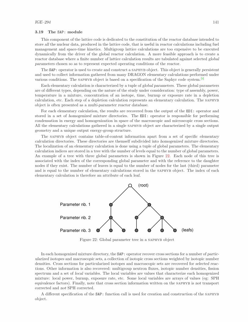
IGE–294 141

3.19 The SAP: module

This component of the lattice code is dedicated to the constitution of the reactor database intended tostore all the nuclear data, produced in the lattice code, that is useful in reactor calculations including fuelmanagement and space-time kinetics. Multigroup lattice calculations are too expensive to be executeddynamically from the driver of the global reactor calculation. A more feasible approach is to create areactor database where a finite number of lattice calculation results are tabulated against selected globalparameters chosen so as to represent expected operating conditions of the reactor.

The SAP: operator is used to create and construct a saphyb object. This object is generally persistentand used to collect information gathered from many DRAGON elementary calculations performed undervarious conditions. The saphyb object is based on a specification of the Saphyr code system.[9]

Each elementary calculation is characterized by a tuple of global parameters. These global parametersare of different types, depending on the nature of the study under consideration: type of assembly, power,temperature in a mixture, concentration of an isotope, time, burnup or exposure rate in a depletioncalculation, etc. Each step of a depletion calculation represents an elementary calculation. The saphyb

object is often presented as a multi-parameter reactor database.

For each elementary calculation, the results are recovered from the output of the EDI: operator andstored in a set of homogenized mixture directories. The EDI: operator is responsible for performingcondensation in energy and homogenization in space of the macroscopic and microscopic cross sections.All the elementary calculations gathered in a single saphyb object are characterized by a single outputgeometry and a unique output energy-group structure.

The saphyb object contains table-of-content information apart from a set of specific elementarycalculation directories. These directories are themself subdivided into homogenized mixture directories.The localization of an elementary calculation is done using a tuple of global parameters. The elementarycalculation indices are stored in a tree with the number of levels equal to the number of global parameters.An example of a tree with three global parameters is shown in Figure 22. Each node of this tree isassociated with the index of the corresponding global parameter and with the reference to the daughternodes if they exist. The number of leaves is equal to the number of nodes for the last (third) parameterand is equal to the number of elementary calculations stored in the saphyb object. The index of eachelementary calculation is therefore an attribute of each leaf.

Parameter nb. 1

Parameter nb. 2

Parameter nb. 3

(root)

(leafs)

Figure 22: Global parameter tree in a saphyb object

In each homogenized mixture directory, the SAP: operator recover cross sections for a number of partic-ularized isotopes and macroscopic sets, a collection of isotopic cross sections weighted by isotopic numberdensities. Cross sections for particularized isotopes and macroscopic sets are recovered for selected reac-tions. Other information is also recovered: multigroup neutron fluxes, isotopic number densities, fissionspectrum and a set of local variables. The local variables are values that characterize each homogenizedmixture: local power, burnup, exposure rate, etc. Some local variables are arrays of values (eg: SPHequivalence factors). Finally, note that cross section information written on the saphyb is not transportcorrected and not SPH corrected.

A different specification of the SAP: function call is used for creation and construction of the saphyb

object.

IGE–294 142

• The first specification is used to initialize the saphyb data structure as a function of the microlib

used in the reference calculation. Optionnally, the homogenized geometry is also provided. Theinitialization call is also used to set the choice of global parameters, local variables, particularizedisotopes, macroscopic sets and selected reactions.

• A modification call to the SAP: function is performed after each elementary calculation in order torecover output information processed by EDI: (condensed and homogenized cross sections) and EVO:

(burnup dependant values). Global parameters and local variables can optionnally be recoveredfrom microlib objects. The EDI: calculation is generally performed with option MICR ALL.


Table 70: Structure (SAP:)

SAPNAM := SAP: [ SAPNAM ] [ HMIC ] :: (saphyb data1)| SAPNAM := SAP: SAPNAM EDINAM [ BRNNAM ] [ HMIC1 [ HMIC2 ] ] [ FLUNAM ]

:: (saphyb data2)| SAPNAM := SAP: SAPNAM SAPRHS :: (saphyb data3)

where

SAPNAM character*12 name of the lcm object containing the master saphyb data structure.

HMIC character*12 name of the reference microlib (type L LIBRARY) containing the micro-scopic cross sections.

EDINAM character*12 name of the lcm object (type L EDIT) containing the edition data struc-ture corresponding to an elementary calculation. The edition data produced by the lastcall to the EDI: module is used.

BRNNAM character*12 name of the lcm object (type L BURNUP) containing the burnup datastructure. This object is compulsory if one of the following parameters is used: IRRA,FLUB and/or TIME.



FLUNAM character*12 name of the reference flux (type L FLUX). By default, the reference fluxis not recovered and not written on the saphyb.

SAPRHS character*12 name of the read-only saphyb data structure. This data structure isconcatenated to SAPNAM using the saphyb data3 data structure, as presented in Sec-tion 3.19.3. SAPRHS must be defined with the same number of energy groups and thesame number of homogeneous regions as SAPNAM . Moreover, all the global and localparameters of SAPRHS must be defined in SAPNAM . SAPNAM may be defined withglobal parameters not defined in SAPRHS.

saphyb data1 input data structure containing initialization information (see Section 3.19.1).

saphyb data2 input data structure containing information related to the recovery of an elementarycalculation (see Section 3.19.2).

saphyb data3 input data structure containing information related to the catenation of a read-onlysaphyb (see Section 3.19.3).

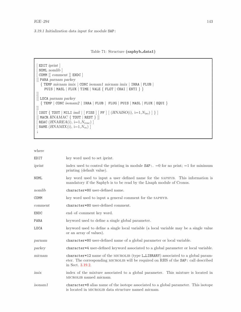
IGE–294 143

3.19.1 Initialization data input for module SAP:

Table 71: Structure (saphyb data1)

[ EDIT iprint ][ NOML nomlib ][ COMM [[ comment ]] ENDC ][[ PARA parnam parkey TEMP micnam imix | CONC isonam1 micnam imix | IRRA | FLUB |PUIS | MASL | FLUX | TIME | VALE FLOT | CHAI | ENTI

]][[ LOCA parnam parkey TEMP | CONC isonam2 | IRRA | FLUB | FLUG | PUIS | MASL | FLUX | EQUI

]][ ISOT TOUT | MILI imil | [ FISS ] [ PF ] [ (HNAISO(i), i=1,Niso) ] ][[ MACR HNAMAC TOUT | REST ]][ REAC (HNAREA(i), i=1,Nreac) ][ NAME (HNAMIX(i), i=1,Nm) ];

where

EDIT key word used to set iprint.

iprint index used to control the printing in module SAP:. =0 for no print; =1 for minimumprinting (default value).

NOML key word used to input a user–defined name for the saphyb. This information ismandatory if the Saphyb is to be read by the Lisaph module of Cronos.

nomlib character*80 user-defined name.

COMM key word used to input a general comment for the saphyb.

comment character*80 user-defined comment.

ENDC end–of–comment key word.

PARA keyword used to define a single global parameter.

LOCA keyword used to define a single local variable (a local variable may be a single valueor an array of values).

parnam character*80 user-defined name of a global parameter or local variable.

parkey character*4 user-defined keyword associated to a global parameter or local variable.

micnam character*12 name of the microlib (type L LIBRARY) associated to a global param-eter. The corresponding microlib will be required on RHS of the SAP: call describedin Sect. 3.19.2.

imix index of the mixture associated to a global parameter. This mixture is located inmicrolib named micnam.

isonam1 character*8 alias name of the isotope associated to a global parameter. This isotopeis located in microlib data structure named micnam.

IGE–294 144

isonam2 character*8 alias name of the isotope associated to a local variable. This isotope islocated in the microlib directory of the edition data structure named EDINAM .

TEMP keyword used to define a temperature (in oC) as global parameter or local variable.

CONC keyword used to define a number density as global parameter or local variable.

IRRA keyword used to define a burnup (in MWday/Tonne) as global parameter or localvariable.

FLUB keyword used to define a fuel-only exposure rate (in n/kb) as global parameter or localvariable. The exposure rate is recovered from the BRNNAM LCM object.

FLUG keyword used to define an exposure rate in global homogenized mixtures (in n/kb) aslocal variable. The exposure rate is recovered from the BRNNAM LCM object.

PUIS keyword used to define the power as global parameter or local variable.

MASL keyword used to define the mass density of heavy isotopes as global parameter or localvariable.

FLUX keyword used to define the volume-averaged, energy-integrated flux as global param-eter or local variable.

TIME keyword used to define the time (in seconds) as global parameter.

EQUI keyword used to define the SPH equivalence factors as local variable. A set of SPHfactors can be defined as local variables. Note that the cross sections and fluxes storedin the saphyb are not SPH corrected.

VALE keyword used to define a user-defined quantity as global parameter. This keywordmust be followed by the type of parameter.

FLOT keyword used to indicate that the user-defined global parameter is a floating pointvalue.

CHAI keyword used to indicate that the user-defined global parameter is a character*12

value.

ENTI keyword used to indicate that the user-defined global parameter is an integer value.

ISOT keyword used to select the set of particularized isotopes.

TOUT keyword used to select all the available isotopes in the reference microlib namedHMIC as particularized isotopes.

MILI keyword used to select the isotopes in the reference microlib named HMIC from aspecific mixture as particularized isotopes.

imil index of the mixture where the particularized isotopes are recovered.

FISS keyword used to select all the available fissile isotopes in the reference microlib namedHMIC as particularized isotopes.

PF keyword used to select all the available fission products in the reference microlib

named HMIC as particularized isotopes.

HNAISO(i) character*12 user-defined isotope name. Niso is the total number of explicitely–selected particularized isotopes.

MACR keyword used to select a type of macroscopic set. A maximum of two macroscopic setsis allowed.

HNAMAC character*8 user-defined name of the macroscopic set.

IGE–294 145

TOUT keyword used to select all the available isotopes in the macroscopic set.

REST keyword used to remove all the particularized isotope contributions from the macro-scopic set.

REAC keyword used to select the set of nuclear reactions.

HNAREA(i) character*4 name of a user-selected reaction. Nreac is the total number of selectedreactions. HNAREA(i) is chosen among the following values:

TOTA Total cross sectionsTOP1 Total P1-weighted cross sectionsABSO Absorption cross sectionsSNNN Excess cross section due to (n,xn) reactionsFISS Fission cross sectionCHI Steady-state fission spectrumNUFI νΣf cross sectionsENER Energy production cross section, taking into account all energy production reactionsEFIS Energy production cross section for (n,f) reaction onlyEGAM Energy production cross section for (n,γ) reaction onlyFUIT B2 times the leakage coefficientSELF within-group P0 scattering cross sectionDIFF scattering cross section for each available Legendre order. These cross sections are

not multiply by the 2ℓ+ 1 factor.PROF profile of the transfer cross section matrices (i.e. position of the non–zero element in

the transfer cross section matrices)TRAN transfer cross section matrices for each available Legendre order. These cross sections

are multiply by the 2ℓ+ 1 factor.CORR transport correction. Note that the cross sections stored in the saphyb are not

transport corrected.STRD STRD cross sections used to compute the diffusion coefficientsNP (n,p) production cross sectionsNT (n,t) production cross sectionsNA (n,α) production cross sections

NAME key word used to define mixture names. By default, mixtures names are of the formHNAMIX(i), where

WRITE(HNAMIX(I),’(3HMIX,I5.5)’) I

HNAMIX(i) Character*20 user-defined mixture name. Nm is the number of mixtures.

3.19.2 Modification data input for module SAP:


[ EDIT iprint ][ CRON ][[ parkey value ]][ ORIG orig ][ SET xtr S | DAY | YEAR ];

IGE–294 146

where

EDIT key word used to set iprint.


CRON key word used to force the kinetics data to be placed into the divers directory. Bydefault, the kinetics data is placed in the cinetique directory of each mixture subdi-rectory. The CRON option can only be used if the Saphyb contains a unique mixture.This option is mandatory if the Saphyb is to be read by the Lisaph module of Cronos.

parkey character*4 keyword associated to a user-defined global parameter.


ORIG key word used to define the father node in the global parameter tree. By default, theindex of the previous elementary calculation is used.

orig index of the elementary calculation associated to the father node in the global param-eter tree.

SET keyword used to recover the flux normalization factor already stored on BRNNAMfrom a sub-directory corresponding to a specific time.

xtr time associated with the current flux calculation. The name of the sub-directory wherethis information is stored will be given by ‘DEPL-DAT’//CNNwhere CNN is a character*4variable defined by WRITE(CNN,’(I4)’) INN where INN is an index associated withthe time xtr.




3.19.3 Modification (catenate) data input for module SAP:


[ EDIT iprint ][ ORIG orig ][[ parkey value ]][ WARNING-ONLY ];

where



parkey character*4 keyword associated to a user-defined global parameter.


IGE–294 147



WARNING-ONLY This option is useful if an elementary calculation in SAPRHS is already present inSAPNAM . If this keyword is set, a warning is send and the SAPNAM values are kept,otherwise the run is aborted (default).

IGE–294 148

3.20 The MC: module

This component of the lattice code is dedicated to the Monte-Carlo solution of the transport equationin multigroup approximation.


Table 74: Structure (MC:)

OUTMC [ TRACK ] := MC: [ OUTMC ] TRACK MICRO | MACRO :: (MC data)

where

OUTMC character*12 name of a Monte-Carlo (type L MC) object open in modification orcreation mode.

TRACK character*12 name of a NXT: tracking (type L TRACK) object open in read-onlyor modification mode. Object TRACK must be constructed with option MC activated(see Section 3.4.3). Opening TRACK in modification mode is useful to add trackinginformation to be plotted with module PSP: (see Section 3.26).

MICRO character*12 name of a microlib (type L LIBRARY) object open in read-only mode.The information on the embedded macrolib is used.

MACRO character*12 name of a macrolib (type L MACROLIB) object open in read-only mode.

MC data input data structure containing specific data (see Section 3.20.1).

3.20.1 Data input for module MC:

Table 75: Structure (MC data)

[ EDIT iprint ]KCODE nsrck ikz kct[ SEED iseed ] [ N2N ][ TALLY

[ MERG COMP | NONE |REGI (iregm(ii),ii=1,nregio) |MIX [ (imixm(ii),ii=1,nbmix) ] ]

[ COND [ NONE | ( icond(ii), ii=1,ngcond) ] ]ENDT ];

where


iprint index used to control the printing in module MC:. =0 for no print; =1 for minimumprinting (default value); =100 to add free-path information in object TRACK (mustbe open in modification mode in that case).

IGE–294 149

KCODE keyword used to define the power iteration settings.

nsrck number of neutrons generated per cycle

ikz number of inactive cycles

kct number of active cycles

SEED keyword used to set the initial seed integer for the random number generator. Bydefault, the seed integer is set from the processor clock.

iseed initial seed integer

N2N keyword used to enable an explicit treatment of (n, 2n) reactions. In this case, N2Ncross sections are expected to be available in the macrolib. By default, (n, 2n) reactionsare taken into account implicitly by the correction on scattering cross sections.

TALLY keyword used to define a tally (macrolib and effective multiplication factor). Using”TALLY ENDT” construct permits to obtain a virtual collision estimation of the effectivemultiplication factor without estimation of the macrolib information.










ENDT keyword used to terminate the definition of a tally.

IGE–294 150

3.21 The T: module

A macrolib object can be defined directly using module MAC: (see Section 3.1) or as part of amicrolib object using module LIB: (see Section 3.2). It is possible to transpose a macrolib using themodule T:. Transposition consists in

• renumbering the energy groups from thermal to fast

• transposing the transfer matrices (SCAT) so that the primary and secondary energy group indicesare permuted

• storing NUSIGF information in CHI and storing CHI infomation in NUSIGF.

A transposed macrolib object permits to make adjoint flux calculations.

The general format of the data for the T: module is the following:

Table 76: Structure (T:)

MACLIB1 := T: MACLIB2 | LIBRARY ;

where

MACLIB1 character*12 name of a the transposed macrolib

MACLIB2 character*12 name of a the original macrolib

LIBRARY character*12 name of a the original microlib containing an embedded macrolib.

IGE–294 151

3.22 The DMAC: module

This module is used to set fixed sources that can be used in the right hand term of an adjoint fixedsource eigenvalue problem. This type of equation appears in generalized perturbation theory (GPT)applications. The fixed sources set in DMAC: are corresponding to the gradient of a reference macrolibwith respect to homogenization and condensation of the cross-section information. The gradient of across section Σ(r) = colΣ1(r) , Σ2(r) with respect to homogenization and condensation is defined as

∇Pφ(ζ); r = Pφ(r)

Σ1(r)〈Σ,φ〉

− 1

〈φ〉Σ2(r)〈Σ,φ〉

− 1

〈φ〉

where the homogenized and condensed cross section is an homogeneous functional of the flux defined as

Pφ(r) =〈Σ,φ〉

〈φ〉.

Each fixed source ∇Pφ(ζ); r is orthogonal to the flux φ(r).


Table 77: Structure (DMAC:)

SOURCE := DMAC: FLUX MICRO | MACRO TRACK :: (DMAC data)

where

SOURCE character*12 name of a fixed sources (type L GPT) object open in creation mode.This object contains a set of adjoint fixed sources corresponding to different macro-regions, macro-groups and cross-section types present in the reference macrolib.

FLUX character*12 name of a reference flux (type L FLUX) object open in read-only mode.

MICRO character*12 name of a reference microlib (type L LIBRARY) object open in read-onlymode. The information on the embedded macrolib is used.

MACRO character*12 name of a reference macrolib (type L MACROLIB) object open in read-only mode.

TRACK character*12 name of a reference tracking (type L TRACK) object open in read-onlymode.

DMAC data input data structure containing specific data (see Section 3.22.1).

3.22.1 Data input for module DMAC:

Table 78: Structure (DMAC data)

[ EDIT iprint ][ RATE

[ MERG COMP | NONE |


IGE–294 152

Structure (DMAC data) continued from last page

REGI (iregm(ii),ii=1,nregio) |MIX [ (imixm(ii),ii=1,nbmix) ] ]

[ COND [ NONE | ( icond(ii), ii=1,ngcond) ] ]ENDR ];

where


iprint index used to control the printing in module DMAC:. =0 for no print; =1 for minimumprinting (default value).

RATE keyword used to define the homogenization and condensation limits.










ENDR keyword used to terminate the definition of the homogenization and condensation.

IGE–294 153

3.23 The DREF: module

This module is used to set fixed sources that can be used in the right hand term of an adjoint fixedsource eigenvalue problem. This type of equation appears in generalized perturbation theory (GPT)applications. The fixed sources set in DREF: are corresponding to the gradient of the RMS functionalwhich is a measure of the discrepancy between actual and reference (or target) power distributions.The actual power distribution is recovered from a MICRO or MACRO object. The reference powerdistribution is recovered from a MICREF or MACREF object.

Actual power values are defined as

Piφ(r) ≡ 〈H,φ〉i =

∫ ∞

0

dE

∫

Vi

d3r H(r, E)φ(r, E)

where the power factors H(r, E) and fluxes φ(r, E) are recovered from H-FACTOR and FLUX-INTG recordsin a macrolib object.

The RMS error on power distribution is an homogeneous functional of the flux defined as

Fφ(r) =∑

i

(

〈H,φ〉i〈H,φ〉

−P ∗i

∑

j P∗j

)2

where the reference (or target) powers P ∗i are obtained from the full-core reference transport calculation.

The gradient of functional Fφ(r) is a G-group function of space defined as

∇Fφ(ζ); r =2

〈H,φ〉

∑

i

(

〈H,φ〉i〈H,φ〉

−P ∗i

∑

j P∗j

)

(

δi(r)−〈H,φ〉i〈H,φ〉

)

H1(r)H2(r)

...HG(r)

where δi(r) = 1 if r ∈ Vi and = 0 otherwise.

Each fixed source ∇Fφ(ζ); r is orthogonal to the flux φ(r).


Table 79: Structure (DREF:)

SOURCE := DREF: FLUX TRACK MICRO | MACRO MICREF | MACREF [ :: [ EDIT iprint ] [ RMS >>RMS VAL<< ] ] ;

where

SOURCE character*12 name of a fixed sources (type L GPT) object open in creation mode.This object contains the adjoint fixed source corresponding to the RMS error on powerdistribution.

FLUX character*12 name of the actual flux (type L FLUX) object open in read-only mode.

TRACK character*12 name of the actual tracking (type L TRACK) object open in read-onlymode.

MICRO character*12 name of the actual microlib (type L LIBRARY) object open in read-onlymode. The information on the embedded macrolib is used.

MACRO character*12 name of the actual macrolib (type L MACROLIB) object open in read-onlymode.

IGE–294 154

MICREF character*12 name of reference (or target) microlib (type L LIBRARY) object openin read-only mode. The information contained in the embedded macrolib is used tocompute P ∗i values.

MACREF character*12 name of reference (or target) macrolib (type L MACROLIB) object openin read-only mode. This information is used to compute P ∗i values.


iprint index used to control the printing in module DREF:. =0 for no print; =1 for minimumprinting (default value).

RMS keyword used to recover the RMS error on power distribution in a CLE-2000 variable.

RMS VAL character*12CLE-2000 variable name in which the extracted RMS value will be placed.

IGE–294 155

3.24 The SENS: module

This module is used to perform an explicit sensitivity analysis of keff to nuclear data represented bythe cross sections.[86] The calculations are performed using adjoint-based first-order-linear perturbationtheory and require the adjoint flux (see Section 3.8). The sensitivity coefficients are stored in a SDF

text file that is compatible with the JAVAPENO module of SCALE[87] (this compatibility is achieved via aslight modification of the rdragon execution script). An example of modification is presented in the filesens.save from the non regression testcase sens.x2m.


Table 80: Structure (SENS:)

SENS.sdf := SENS: FLUNAM ADJ FLUNAM TRKNAM MACRO :: (SENS data)

where

SENS.sdf character*12 name of a SDF file object that is created by SENS:.

FLUNAM character*12 name of the required flux (type L FLUX) object open in read-only mode.

ADJ FLUNAM character*12 name of the required adjoint flux (type L FLUX) object open in read-only mode.

TRKNAM character*12 name of the required tracking (type L TRACK) object open in read-onlymode.

MACRO character*12 name of the required macrolib (type L MACROLIB) object open in read-only mode.

SENS data input data structure containing specific data (see Section 3.24.1).

3.24.1 Data input for module SENS:

Table 81: Structure (SENS data)

[ EDIT iprint ][ ANIS nanis ];

where


iprint index used to control the printing in module SENS:. =0 for no print; =1 for minimumprinting (default value).

ANIS keyword used to specify the level naniso of anisotropy permitted in the calculation.

nanis number of Legendre orders for the representation of the scattering cross sections andthe anisotropy of the flux. The default value is nanis=1 corresponding to the use

IGE–294 156

of isotropic scattering cross sections and integrated flux. The number of Legendreorders used for the sensitivity calculations is the lowest between nanis and the level ofanisotropy available in the MACRO data.

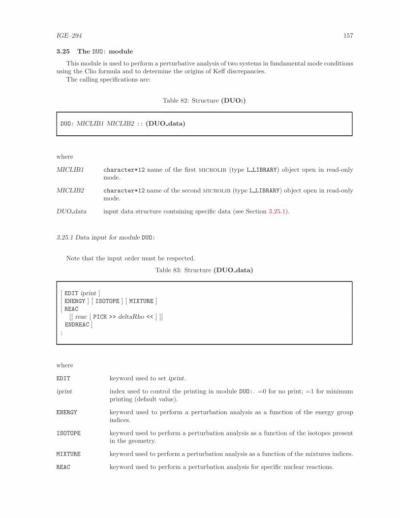
IGE–294 157

3.25 The DUO: module

This module is used to perform a perturbative analysis of two systems in fundamental mode conditionsusing the Clio formula and to determine the origins of Keff discrepancies.


Table 82: Structure (DUO:)

DUO: MICLIB1 MICLIB2 :: (DUO data)

where

MICLIB1 character*12 name of the first microlib (type L LIBRARY) object open in read-onlymode.

MICLIB2 character*12 name of the second microlib (type L LIBRARY) object open in read-onlymode.

DUO data input data structure containing specific data (see Section 3.25.1).

3.25.1 Data input for module DUO:

Note that the input order must be respected.

Table 83: Structure (DUO data)

[ EDIT iprint ][ ENERGY ] [ ISOTOPE ] [ MIXTURE ][ REAC

[[ reac [ PICK >> deltaRho << ] ]]ENDREAC ]

;

where


iprint index used to control the printing in module DUO:. =0 for no print; =1 for minimumprinting (default value).

ENERGY keyword used to perform a perturbation analysis as a function of the energy groupindices.

ISOTOPE keyword used to perform a perturbation analysis as a function of the isotopes presentin the geometry.

MIXTURE keyword used to perform a perturbation analysis as a function of the mixtures indices.

REAC keyword used to perform a perturbation analysis for specific nuclear reactions.

IGE–294 158

reac character*8 name of a nuclear reaction σx. The reactivity effect is computed usingthe formula

δλx =(φ∗1)

⊤δ Sx φ2

(φ∗1)⊤ P2 φ2

. (3.34)

where Sx is a matrix containing the the contributions of the reaction σx. The othersymbols are defined in Sect. 3.25.2. Examples of reaction names are:

NTOT0: total cross section

NG: radiative capture cross section

N2N: (n,2n) cross section

NFTOT: fission cross section

NELAS: elastic scattering cross section

SCAT00: scattering matrix

NUSIGF: dyadic product of the fission spectrum times ν fission cross section

LEAK: neutron leakage

The balance relation for the global reactivity effect is

δλ = δλNTOT0 − δλSCAT00 −δλNUSIGFKeff

+ δλLEAK (3.35)

where Keff is the effective multiplication factor.

PICK keyword used to recover the delta-rho discrepancy for reaction reac in a CLE-2000variable.

deltaRho character*12 CLE-2000 variable name in which the extracted delta-rho discrepancywill be placed.

ENDREAC keyword used to indicate that no more nuclear reactions will be analysed.

3.25.2 Theory

The module DUO: is an implementation of the clio perturbative analysis method, as introduced inRef. 92. This method is useful for comparing two similar systems in fundamental mode conditions. It isbased on fundamental mode balance equations that must be satisfied by the direct and adjoint solutionsof each of the two systems. The balance equation of the first system is written

L1φ1 − λ1 P1 φ1 = 0 and L⊤1 φ∗1 − λ1 P

⊤1 φ∗1 = 0 (3.36)

where

L1 = absorption (total plus leakage minus scattering) reaction rate matrix

P1 = production (nu times fission) reaction rate matrix

λ1 = one over the effective multiplication factor

φ1 = direct multigroup flux in each mixture of the geometry

φ∗1 = adjoint multigroup flux in each mixture of the geometry.

IGE–294 159

Similarly, the balance equation of the second system is written

L2φ2 − λ2 P2 φ2 = 0. (3.37)

Next, we write

L2 = L1 + δ L P2 = P1 + δP , φ2 = φ1 + δφ and λ2 = λ1 + δλ. (3.38)

Substituting Eq. (3.38) into Eq. (3.37), we write

L1φ1 + L1δφ+ δ L φ2 − [λ1 P1 φ1 + λ1 P1 δφ+ (λ2 P2 −λ1 P1)φ2] = 0. (3.39)

Following the guideline from Ref. 92, we subtract Eq. (3.36) from Eq. (3.39) to obtain

(L1 − λ1 P1) δφ = (−δ L+λ2 P2 −λ1 P1)φ2 (3.40)

Next, we left-multiply this matrix system by a row vector equal to (φ∗1)⊤, in order to make the LHS

vanishing. This operation is written

(φ∗1)⊤(L1 − λ1 P1) δφ = (φ∗1)

⊤(−δ L+λ2 P2 −λ1 P1)φ2 = 0 (3.41)

because

(φ∗1)⊤(L1 − λ1 P1) = 0⊤ (3.42)

in term of Eq. (3.36).

Using the relation λ2 P2 −λ1 P1 = δλ P2 +λ1 δP, Eq. (3.41) can be rewritten as

(φ∗1)⊤(−δ L+δλ P2 +λ1 δP)φ2 = 0 (3.43)

so that

δλ =(φ∗1)

⊤(δ L−λ1 δP)φ2

(φ∗1)⊤ P2 φ2

. (3.44)

Equation 3.44 is not a first order perturbation approximation of δλ; it is an exact expression of it.Its numerator is used to obtain every component of δλ in term of energy group, isotope, mixture and/ornuclear reaction.

IGE–294 160

3.26 The PSP: module

The PSP:module is used to generate a graphical file in a PostScript ASCII format for a DRAGON 2-Dgeometry which can be analyzed using the EXCELT: or NXT: tracking module (see Sections. 3.4.2 and 3.4.3).The module PSP: is based on the PSPLOT Fortran library from Nova Southeastern University.[77] Sinceonly a few PSPLOT routines were required and because additional PostScript routine not present in theoriginal package were needed, the routines have been completely readapted to DRAGON. These routinesare no longer machine dependent. The PostScript files generated by DRAGON can be viewed by anyPostScript viewer, such as Ghostview[78] or sent to a printer compatible with this language. In DRAGONthe PSP: module is activated using the following list of commands:

Table 84: Structure (PSP:)

PSGEO := PSP: PSGEO GEONAM | TRKNAM [ FLUNAM ] :: (descpsp)

where

PSGEO character*12name of the file that will contain the graphical description in a POSTSCRIPTformat. This file must have a sequential ASCII format.

GEONAM character*12 name of a read-only geometry (see Section Section 3.3).

TRKNAM character*12name of an NXT or EXCELL type read-only tracking (see Sections. 3.4.2and 3.4.3).

FLUNAM character*12 name of an optional read-only fluxunk (see Section 3.8). It is requiredonly if a flux mapping plot is requested.

(descpsp) structure containing the input data to this module (see Section 3.26.1).

3.26.1 Data input for module PSP:

Table 85: Structure (descpsp)

[ EDIT iprint ][ FILL NONE | GRAY | RGB | CMYK | HSB [ NOCONTOUR ] ][ TYPE REGION | MIXTURE | FLUX | MGFLUX ]

where


iprint index used to control the printing in this module. It must be set to 0 if no printing onthe output file is required.

FILL keyword to specify the drawing options.

NONE keyword to specify that only region contour are to be drawn.

IGE–294 161

GRAY keyword to specify that the regions will be filled with various levels of gray.

RGB keyword to specify that the regions will be filled with various colors taken using theRGB color scheme.

CMYK keyword to specify that the regions will be filled with various colors taken using theCMYK color scheme.

HSB keyword to specify that the regions will be filled with various colors taken using theHSB color scheme. This is the default option.

NOCONTOUR keyword to specify that the contour lines delimiting each region will not be drawn.

TYPE keyword to specify the type of graphics generated.

REGION keyword to specify that different colors or gray levels will be associated with eachregion. This is the default option.

MIXTURE keyword to specify that different colors or gray levels will be associated with eachmixture.

FLUX keyword to specify that the group integrated flux is to be drawn.

MGFLUX keyword to specify that the group flux is to be drawn.

IGE–294 162

4 THE UTILITY MODULES

DRAGON contains a number of utility modules used to perform tasks not related to reactor physics.These modules are also available to any code built around the GAN generalized driver.[6]

4.1 The equality module

This module is used to duplicate a lcm object. The calling specifications are:

Table 86: Structure (equality)

NAME1 := [ NAME1 ] NAME2[ :: [ EDIT iprint ] [ OLD | SAP ] [[ STEP UP NOMDIR | AT index ]] ] ;

NAME1 character*12 name of the output data structure. It can be a lcm object (eithermemory-resident or xsm-based), a sequential binary file or a sequential ascii file. IfNAME1 is a lcm object and if it appears on both sides, it is erased and refilled withthe contents of NAME2 .

NAME2 character*12 name of the input data structure. It can be a lcm object (eithermemory-resident or xsm-based), a sequential binary file or a sequential ascii file.



OLD keyword used to import/export a LHS sequential ascii file in 1995 lcm specification.By default, the up-to-date specification is used.

SAP keyword used to import/export a LHS sequential ascii file in Saphyr lcm specification.

STEP keyword used to move in the lcm object hierarchy of NAME2 before making the copy.

UP keyword used to move up towards a sub-directory of NAME2 of the active directory.

NOMDIR copy the information located in the sub-directory named NOMDIR.

AT keyword used to move up towards a component in an heterogeneous list of NAME2 .

index copy the information located in the index–th component of the heterogeneous list.

If both the RHS and LHS are lcm objects (either memory-resident or xsm-based), a single copy isperformed. A memory-resident lcm object can be created from an xsm file or an xsm file can be createdfrom a memory-resident lcm object. If the LHS is a sequential file and the RHS is a lcm object, an exportis performed. The export format is either binary or ASCII. If the LHS is a lcm object and the RHS isa sequential file, an import is performed. The case where both the LHS and the RHS are sequential filesis not supported.

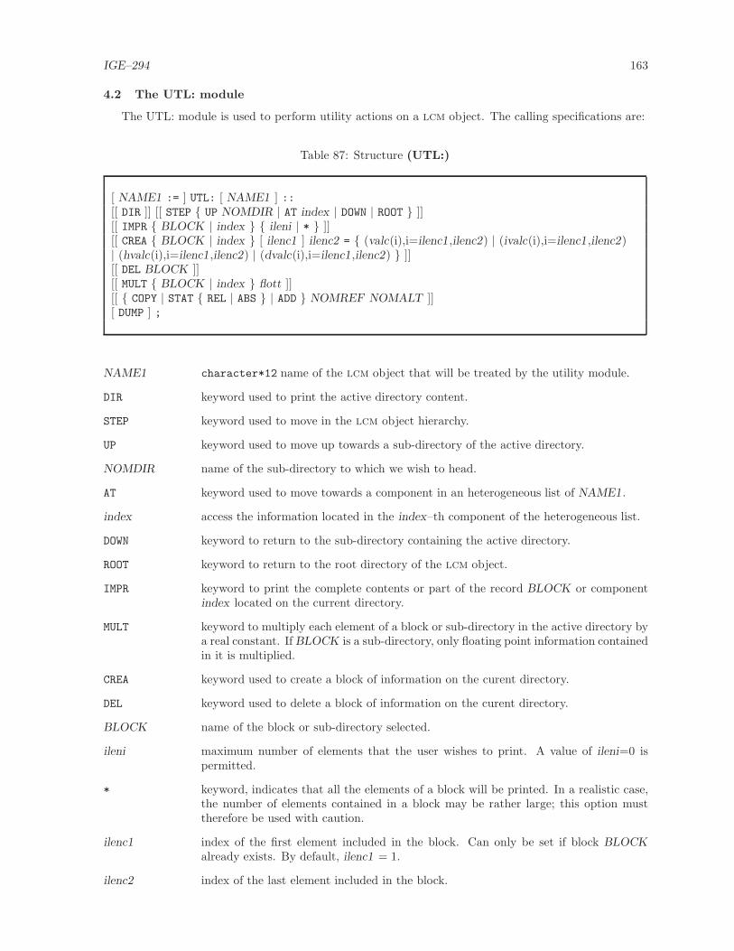
IGE–294 163

4.2 The UTL: module

The UTL: module is used to perform utility actions on a lcm object. The calling specifications are:

Table 87: Structure (UTL:)

[ NAME1 := ] UTL: [ NAME1 ] ::[[ DIR ]] [[ STEP UP NOMDIR | AT index | DOWN | ROOT ]][[ IMPR BLOCK | index ileni | * ]][[ CREA BLOCK | index [ ilenc1 ] ilenc2 = (valc(i),i=ilenc1 ,ilenc2) | (ivalc(i),i=ilenc1 ,ilenc2)| (hvalc(i),i=ilenc1 ,ilenc2) | (dvalc(i),i=ilenc1 ,ilenc2) ]][[ DEL BLOCK ]][[ MULT BLOCK | index flott ]][[ COPY | STAT REL | ABS | ADD NOMREF NOMALT ]][ DUMP ] ;

NAME1 character*12 name of the lcm object that will be treated by the utility module.

DIR keyword used to print the active directory content.

STEP keyword used to move in the lcm object hierarchy.

UP keyword used to move up towards a sub-directory of the active directory.

NOMDIR name of the sub-directory to which we wish to head.

AT keyword used to move towards a component in an heterogeneous list of NAME1 .

index access the information located in the index–th component of the heterogeneous list.

DOWN keyword to return to the sub-directory containing the active directory.

ROOT keyword to return to the root directory of the lcm object.

IMPR keyword to print the complete contents or part of the record BLOCK or componentindex located on the current directory.

MULT keyword to multiply each element of a block or sub-directory in the active directory bya real constant. If BLOCK is a sub-directory, only floating point information containedin it is multiplied.

CREA keyword used to create a block of information on the curent directory.

DEL keyword used to delete a block of information on the curent directory.

BLOCK name of the block or sub-directory selected.

ileni maximum number of elements that the user wishes to print. A value of ileni=0 ispermitted.

* keyword, indicates that all the elements of a block will be printed. In a realistic case,the number of elements contained in a block may be rather large; this option musttherefore be used with caution.

ilenc1 index of the first element included in the block. Can only be set if block BLOCKalready exists. By default, ilenc1 = 1.

ilenc2 index of the last element included in the block.

IGE–294 164

= keyword, indicates that the input values will follow.

valc real vector containing the information to be written in the record BLOCK .

ivalc integer vector containing the information to be written in the record BLOCK .

hvalc character*4 array containing the information to be written in the record BLOCK .

dvalc double precision array containing the information to be written in the record BLOCK .

flott constant by which a block or sub-directory will be multiplied.

COPY keyword used to copy an existing record or sub-directory onto a new record or sub-directory.

ADD keyword used to add the contents of two records or two sub-directories. If NOMREFand NOMALT are two sub-directories, only the floating point information containedin them is added. The result is written into NOMALT.

STAT keyword used to compare the contents of two records.

REL the relative differences are printed.

ABS the absolute differences are printed.

NOMREF name of the reference block.

NOMALT name of the block which may possibly be modified during the ADD and COPY operations.

DUMP Dump the active directory of and its sub-directories to the printer.

IGE–294 165

4.3 The DELETE: module

This module is used to delete one or many lcm objects. The calling specifications are:

Table 88: Structure (DELETE:)

[[ NAME1 ]] := DELETE: [[ NAME1 ]] ;

NAME1 character*12 name of a lcm object.

The names of the lcm object should be present on both the LHS and the RHS. A lcm object namedPARENT can be deleted using the following command:

PARENT := DELETE: PARENT ;

IGE–294 166

4.4 The BACKUP: module

This module is used to copy one or many lcm objects (memory-resident or xsm-based), along withall of its parent to a backup lcm object. The backup data structure can be stored on a single lcm object(either memory-resident or xsm-based), a sequential binary file or a sequential ASCII file. The callingspecifications are:

Table 89: Structure (BACKUP:)

NAME1 := BACKUP: [ NAME1 ] [[ NAME2 ]] [ ::[ EDIT iprint ][[ STEP UP NOMDIR | AT index ]] ] ;

NAME1 character*12 name of lcm object used as a backup media.

NAME2 character*12 name of lcm object to be transfer to the backup lcm object. This lcmobject must be in a memory-resident or xsm-based format.



STEP keyword used to move in the lcm object hierarchy of NAME2 before making thebackup.


NOMDIR backup the information into the sub-directory named NOMDIR.


index backup the information into the index–th component of the heterogeneous list.

If NAME1 appears only on the LHS, it is created. If NAME1 appears on both the LHS and the RHS,it is updated.

IGE–294 167

4.5 The RECOVER: module

This module is used to recover from a backup lcm object (see Section 4.4) one or many lcm objects(memory-resident or xsm-based). The calling specifications are:

Table 90: Structure (RECOVER:)

[[ NAME1 ]] := RECOVER: NAME2 [[ NAME1 ]] [ ::[ EDIT iprint ][[ STEP UP NOMDIR | AT index ]] ] ;

NAME1 character*12 name of the lcm objects that are to be recovered.

NAME2 character*12 name of a backup lcm object.



STEP keyword used to move in the lcm object hierarchy of NAME2 before making therecover.


NOMDIR recover the information located in the sub-directory named NOMDIR.


index recover the information located in the index–th component of the heterogeneous list.

If NAME1 appears only on the LHS, it is created. If NAME1 appears on both the LHS and the RHS,it is replaced by the information located on the backup media.

IGE–294 168

4.6 The ADD: module

This module is used to add the floating point information contained of the two lcm object locatedon the RHS. The result is stored in a third output lcm object. The calling specifications are:

Table 91: Structure (ADD:)

NAME1 := ADD: NAME2 NAME3 ;

NAME1 character*12 name of a lcm object which contains the final information.

NAME2 character*12 name of a lcm object which contains the first part of the initial infor-mation. One can use NAME2=NAME1 .

NAME3 character*12 name of a lcm object which contains the second part of the initialinformation.

IGE–294 169

4.7 The MPX: module

This module is used to multiply the floating point information contained in a lcm object located onthe RHS by a user-defined real number. The result is stored in a second output lcm object. The callingspecifications are:

Table 92: Structure (MPX:)

NAME1 := MPX: NAME2 :: real ;

NAME1 character*12 name of a lcm object which contains the final information.

NAME2 character*12 name of a lcm object which contains the the initial information. Onecan use NAME2=NAME1 .

real real number used as a multiplication factor.

IGE–294 170

4.8 The STAT: module

This module is used to compare the floating point information contained in two different lcm object.The calling specifications are:

Table 93: Structure (STAT:)

STAT: NAME1 NAME2 ;

NAME1 character*12 name of the reference lcm object.

NAME2 character*12 name of a compared lcm object.

IGE–294 171

4.9 The GREP: module

The GREP: module is used to extract a single value from a lcm object. The calling specificationsare:

Table 94: Structure (GREP:)

GREP: NAME3 ::

[ EDIT iprint ][[ STEP UP NOMDIR | AT index ]][[ TYPE BLOCK | index >>itype<< ]][[ GETVAL | MAXVAL | MINVAL | INDMAX | INDMIN | MEAN BLOCK | index index1 [ index2 | * [ index3 ] | NVAL neval | * ][[ >>value<< ]]

]] ;

NAME3 character*12 name of the lcm object from which extractions will be performed.


iprint index set to 1 to enable printing in this module. By default, iprint = 0.

STEP keyword used to move in the lcm object hierarchy.

UP keyword used to move up towards a sub-directory of the active directory.

NOMDIR name of the sub-directory or heterogeneous list to which we wish to head.

AT keyword used to move up towards a component in the heterogeneous list.

index access the information located in the index–th component of the heterogeneous list.

BLOCK name of the record which will be analyzed by the GREP: utility.

index index of the record which will be analyzed by the GREP: utility.

TYPE keyword used to get the lcm type of record BLOCK .

itype type of block BLOCK or list component index (= 1: integer; = 2: real; = 3: character;= 4: double precision; = 5: logical; = 10: list; = 99: undefined).

GETVAL keyword used to get values from an existing record. The receiving CLE-2000 variablesare assumed to be of the same type as the picked values (all CLE-2000 types aresupported).

MAXVAL keyword used to get the maximum value of an existing record. The receiving CLE-2000 single variable is assumed to be of the same type as the picked maximum (validfor integer, real and double precision types).

MINVAL keyword used to get the minimum value of an existing record. The receiving CLE-2000single variable is assumed to be of the same type as the picked minimum (valid forinteger, real and double precision types).

INDMAX keyword used to get the index (position inside the block) of the maximum value of anexisting record. The receiving CLE-2000 single variable is assumed of an integer type(valid for integer, real and double precision blocks).

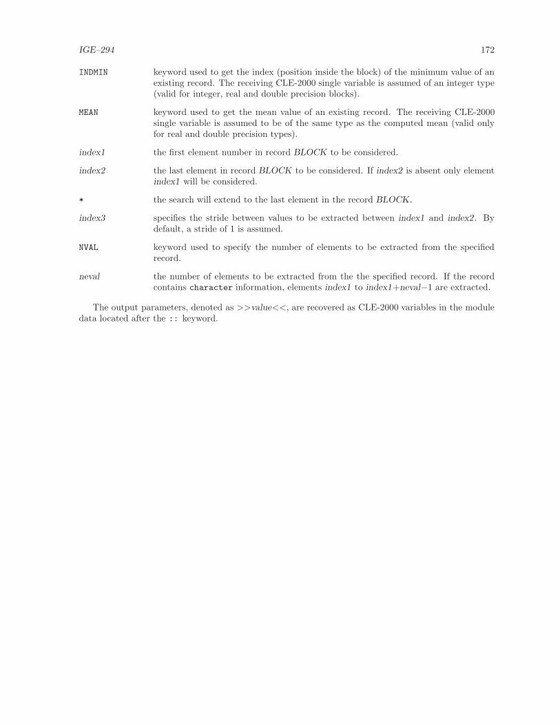
IGE–294 172

INDMIN keyword used to get the index (position inside the block) of the minimum value of anexisting record. The receiving CLE-2000 single variable is assumed of an integer type(valid for integer, real and double precision blocks).

MEAN keyword used to get the mean value of an existing record. The receiving CLE-2000single variable is assumed to be of the same type as the computed mean (valid onlyfor real and double precision types).

index1 the first element number in record BLOCK to be considered.

index2 the last element in record BLOCK to be considered. If index2 is absent only elementindex1 will be considered.

* the search will extend to the last element in the record BLOCK .

index3 specifies the stride between values to be extracted between index1 and index2 . Bydefault, a stride of 1 is assumed.

NVAL keyword used to specify the number of elements to be extracted from the specifiedrecord.

neval the number of elements to be extracted from the the specified record. If the recordcontains character information, elements index1 to index1+neval−1 are extracted.

The output parameters, denoted as >>value<<, are recovered as CLE-2000 variables in the moduledata located after the :: keyword.

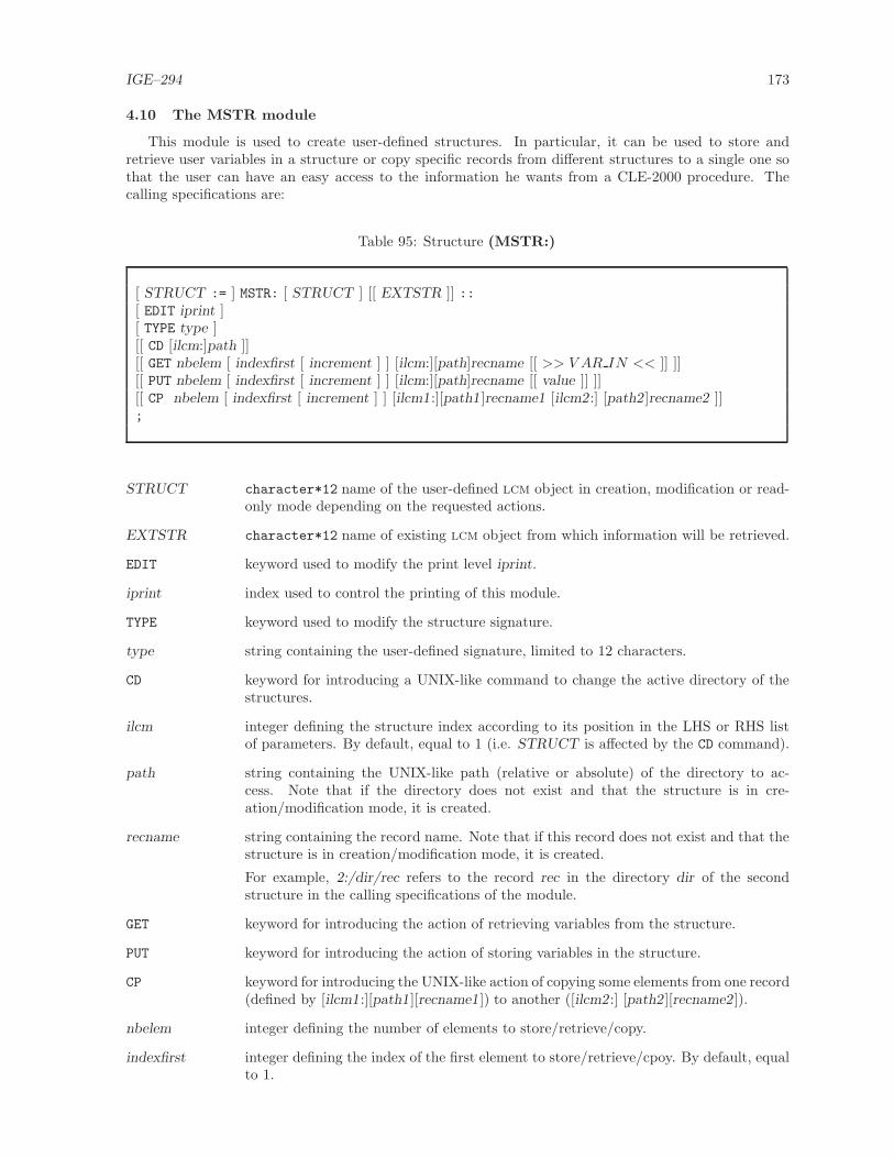
IGE–294 173

4.10 The MSTR module

This module is used to create user-defined structures. In particular, it can be used to store andretrieve user variables in a structure or copy specific records from different structures to a single one sothat the user can have an easy access to the information he wants from a CLE-2000 procedure. Thecalling specifications are:

Table 95: Structure (MSTR:)

[ STRUCT := ] MSTR: [ STRUCT ] [[ EXTSTR ]] ::[ EDIT iprint ][ TYPE type ][[ CD [ilcm:]path ]][[ GET nbelem [ indexfirst [ increment ] ] [ilcm:][path]recname [[ >> V AR IN << ]] ]][[ PUT nbelem [ indexfirst [ increment ] ] [ilcm:][path]recname [[ value ]] ]][[ CP nbelem [ indexfirst [ increment ] ] [ilcm1 :][path1 ]recname1 [ilcm2 :] [path2 ]recname2 ]];

STRUCT character*12 name of the user-defined lcm object in creation, modification or read-only mode depending on the requested actions.

EXTSTR character*12 name of existing lcm object from which information will be retrieved.


iprint index used to control the printing of this module.

TYPE keyword used to modify the structure signature.

type string containing the user-defined signature, limited to 12 characters.

CD keyword for introducing a UNIX-like command to change the active directory of thestructures.

ilcm integer defining the structure index according to its position in the LHS or RHS listof parameters. By default, equal to 1 (i.e. STRUCT is affected by the CD command).

path string containing the UNIX-like path (relative or absolute) of the directory to ac-cess. Note that if the directory does not exist and that the structure is in cre-ation/modification mode, it is created.

recname string containing the record name. Note that if this record does not exist and that thestructure is in creation/modification mode, it is created.

For example, 2:/dir/rec refers to the record rec in the directory dir of the secondstructure in the calling specifications of the module.

GET keyword for introducing the action of retrieving variables from the structure.

PUT keyword for introducing the action of storing variables in the structure.

CP keyword for introducing the UNIX-like action of copying some elements from one record(defined by [ilcm1 :][path1 ][recname1 ]) to another ([ilcm2 :] [path2 ][recname2 ]).

nbelem integer defining the number of elements to store/retrieve/copy.

indexfirst integer defining the index of the first element to store/retrieve/cpoy. By default, equalto 1.

IGE–294 174

increment integer defining the stride in the record between the values to be stored/retrieved/copied.By default, equal to 1.

V AR IN character*12 CLE-2000 variable name in which the extracted value will be placed.It is expected that the number of values extracted and the number (and types) ofvariables agree.

value value to be stored. The first one defines the record type and all the values should beof the same type.

IGE–294 175

4.11 The FIND0: module

The FIND0: module is used to find the root of a function using the Brent’s method. This procedureassumes that the zero is bracketed in an interval given in the input using the two first points, and thatthe function used is continuous in this interval. The calling specifications are:

Table 96: Structure (FIND0:)

L0 := FIND0: [ L0 ] :: [ DEBUG ] [ ITMAX itmax ] [ TOL tol ] POINT X x1 Y y1 POINT X x2 Y y2 | Y y3 >>lFlag<< >>rRoot<< ;

L0 character*12 names of the FIND0 lcm object (type L 0) that will contain all in-formation necessary for the zero-finding procedure. If L0 appears on both sides, it isupdated; otherwise, it is created.

DEBUG keyword used to edit the content of most variables in FIND0; used only for debuggingpurposes.

ITMAX keyword used to specify the maximum number of iterations that will be allowed forthe zero-finding procedure. The procedure will abort if the number of iterations goesbeyond this maximum value.

itmax the maximum number of iterations. Default value: 100.

TOL keyword used to specify the tolerance on the zero to be found.

tol tolerance. Default value: 1.E-5.

POINT keyword used to specify that the next point will be given.

X keyword used to specify that an abscissa will be given.

Y keyword used to specify that an ordinate will be given.

x1 the first abscissa value.

y1 the first ordinate value.

x2 the second abscissa value.

y2 the second ordinate value.

y3 in the case we are in an update mode, only a new ordinate value is given.

lFlag CLE-2000 logical variable in writable mode. The value returned is true if the newguessed root is within tol, false otherwise.

rRoot CLE-2000 real variable in writable mode. The value returned is the last guess for theroot.

Note that the zero-finding procedure has an initial mode where NAME1 , NAME2 and NAME3 arecreated. In the initialization process, the two points specifying the interval must be given, and it isexpected that y1×y2< 0. In the updated mode, there is no need to put back the abscissa of the nextpoint because it is expected to be the last real value that was generated by the procedure. This explainswhy you will only input Y y3 .

The FIND0 specification is used to store intermediate values needed by the zero-finding procedure.There are no directories in this object, and it is created and updated only by the FIND0: module. Tounderstand the content of the object, it is possible, using the labels given for every block, to refer toBrent’s algorithm.[74].

IGE–294 176

4.12 The ABORT: module

This module is used to abort the overall calculation, calling the XABORT() subroutine from the Ganlib.

Table 97: Structure (ABORT:)

ABORT: ;

IGE–294 177

4.13 The END: module

This module is used to delete all the memory-resident lcm objects, to close all the remaining localfiles and to return from a procedure or to stop the run. The calling specifications are:

Table 98: Structure (END:)

END: ;

IGE–294 178

5 THE MPI MODULES

DRAGON contains two modules that enables MPI capabilities. These modules are also available toany code built around the GAN generalized driver[6], provided that it is properly compiled.

5.1 The DRVMPI: module

This module is a utility module related to MPI. It is mostly used to know the rank of the node runningthe current script. The calling specifications are:

Table 99: Structure (DRVMPI:)

[ NAME := ] DRVMPI: :: [ EDIT iprint ] [ WORLD-SIZE >>ncpu<< ] [ MY-ID >>rank<< ][[ SETLOOP B0 | B1 len >>beg<< >>end<< ]][ ALLREDUCE SUM | PROD | MAX | MIN operand >>result<< ][ TIME >>dTime<< ] [ BARRIER ] ;

NAME character*12 name of a dummy data structure to be possibly used as NAME2 in theSNDMPI: module. It can be a linked list or an XSM file.



WORLD-SIZE keyword used to recover ncpu.

ncpu total number of nodes in the MPI environment.

MY-ID keyword used to recover rank.

rank rank of the node that is running the script.

SETLOOP keyword used to partition the set 0 · · ·len−1 or 1 · · ·len equitably over the nodes.The result beg · · ·end is different for each node.

B0 keyword used to set the intial position to 0.

B1 keyword used to set the intial position to 1.

len set length.

beg beginning of the set for the current script. Must be an integer variable.

end end of the set for the current script. Must be an integer variable.

ALLREDUCE keyword used to make a computation over all the operand and to store the result inresult. Problems can be encountered in the 64-bits version.

SUM keyword used to make ALLREDUCE perform a summation.

PROD keyword used to make ALLREDUCE perform a multiplication.

MAX keyword used to make ALLREDUCE find the maximum over all operand.

MIN keyword used to make ALLREDUCE find the maximum over all operand.

operand operand in the ALLREDUCE calculation. Cannot be a string or a logical value.

IGE–294 179

result result of the ALLREDUCE calculation. Must be a variable of the same type as operand.

TIME keyword used to recover dTime.

dTime time in seconds since an arbitrary time in the past. Must be a double precision variable.

BARRIER keyword used to stop the calculation until every node has reach this barrier.

NAME is always empty. What matters is that NAME is no more only declared, it now exists afterthe call of DRVMPI: module.

The output parameters, denoted as >>value<<, are recovered as CLE-2000 variables in the moduledata located after the :: keyword.

5.2 The SNDMPI: module

This module is used to send or receive a linked list or an XSM file from one node to another onethanks to MPI. It is possible to send a linked list into an XSM file and vice versa. The module is blockeduntil the message is sent or received. The calling specifications are:

Table 100: Structure (SNDMPI:)

[ NAME1 := ] SNDMPI: [ NAME2 ] :: [ EDIT iprint ] FROM iFrom TO iTo | ALL [ ITEM from >>to<< ] ;

NAME1 character*12 name of the data structure that will be received. It can be a linked listor an XSM file.

NAME2 character*12 name of the data structure that will be sent. It can be a linked list oran XSM file. Since on the RHS, it has to exist even for receiving scripts. In this case itis recommanded to create an empty data structure NAME2 by calling the DRVMPI:module.



FROM keyword used to set iFrom.

iFrom rank of the node from which NAME2 has to be read.

TO keyword used to set iTo.

iTo rank of the node where NAME1 has to be written.

ALL keyword to make every node receive NAME2 except the node iFrom.

ITEM keyword used to send the value from to to either on iTo or ALL nodes. NAME1 andNAME2 are optional since they will be ignored.

from value to send. Can be an integer, a real, a double or a logical.

to variable used to receive from value. Must match from type.

IGE–294 180

6 EXAMPLES

We will now present a few examples of DRAGON input structures in such as to clarify and illustratesome of the options presented in Sections 3 and 4. These examples are non-regression testcases used toensure that existing capabilities of Dragon are not lost with subsequent updates of the code. They makeuse of two assert procedures defined in CLE-2000 language, assertS and assertV, defined in Section 6.7.These procedures are generally not used in computational schemes.

6.1 Scattering cross sections

In DRAGON, the angular dependence of the scattering cross section is expressed in a Legendre seriesexpansion of the form:

Σs(Ω · Ω′) = Σs(µ) =

L∑

l=0

(

(2l + 1)

4π

)

Σs,lPl(µ).

Since the Legendre polynomials satisfy the following orthogonality conditions:

∫ 1

−1

dµPl(µ)Pm(µ) =

(

2δl,m(2l + 1)

)

,

we will have

Σs,l =

∫ 1

−1

dµ

∫ 2π

0

dϕΣs(µ)Pl(µ) = 2π

∫ 1

−1

dµΣs(µ)Pl(µ).

Let us now consider the following three-group (ngroup=3) isotropic and linearly anisotropic scatteringcross sections (L=naniso=2) given by:

l g Σg→1s,l (cm−1) Σg→2

s,l (cm−1) Σg→3s,l (cm−1)

1 0.90 0.80 0.000 2 0.00 0.70 0.60

3 0.00 0.30 0.401 0.09 0.05 0.08

1 2 0.00 0.07 0.063 0.03 0.00 0.04

In DRAGON this scattering cross section must be entered as

SCAT (* L=0 *) 1 1 (* 3->1 *) (* 2->1 *) (* 1->1 *) 0.90

3 3 (* 3->2 *) 0.30 (* 2->2 *) 0.70 (* 1->2 *) 0.80

2 3 (* 3->3 *) 0.40 (* 2->3 *) 0.60 (* 1->3 *)

SCAT (* L=1 *) 3 3 (* 3->1 *) 0.03 (* 2->1 *) 0.00 (* 1->1 *) 0.09

2 2 (* 3->2 *) (* 2->2 *) 0.07 (* 1->2 *) 0.05

3 3 (* 3->3 *) 0.04 (* 2->3 *) 0.06 (* 1->3 *) 0.08

6.2 Geometries

In order to illustrate the use of the various geometries presented in Section 3.3, lets us consider a fewexamples that can be treated by DRAGON.

• 1–D Slab geometry (see Figure 23):

This geometry can be analyzed using a SYBILT: tracking modules:

PLATE := GEO: :: CAR1D 6

X- VOID X+ ALBE 1.2

MESHX 0.0 0.1 0.3 0.5 0.6 0.8 1.0

SPLITX 2 2 2 1 2 1

MIX 1 2 3 4 5 6 ;

IGE–294 181

0.0 0.1 0.3 0.5 0.6

β=0.0 β=1.2

X

0.8 1.0

Figure 23: Slab geometry with mesh-splitting

β=1

X

CL

CL

CL

Figure 24: Two-dimensional Cartesian assembly containing micro-structures

• 2–D Cartesian geometry containing micro-structures (see figure Figure 24):

This geometry can be analyzed only using SYBILT: tracking modules:

CARNSG := GEO: :: CAR2D 3 3

X- DIAG X+ REFL Y- SYME Y+ DIAG

MIX C1 C1 C2

C3 C2

C3

BIHET SPHE (*NG=*) 2 (* NMILG= *) 2 (* SPHERICAL MICRO-STRUCTURE *)

(* NS= *) 3 3

(* M-S-1 *) 0.0 0.1 0.2 0.3 (* M-S 2 *) 0.0 0.2 0.4 0.5

(* COMPOSITE MIXTURES *) 4 5

(* MIXTURES SURROUNDING M-S *) 1 1

(* COMPOSITE MIXTURE 4 FRACT *) 0.4 0.0

(* REAL MIXTURE CONTENT M-S-1 *) 3 1 3

(* COMPOSITE MIXTURE 5 FRACT *) 0.2 0.1



::: C1 := GEO: CAR2D 1 1 (* HOMOGENEOUS CELL WITH M-S *)

MESHX 0.0 1.45 MESHY 0.0 1.45 MIX 4 ;

::: C2 := GEO: C1 (* HOMOGENEOUS CELL WITHOUT M-S *)

MIX 1 ;

::: C3 := GEO: CARCEL 2 (* CELL WITH M-S TUBE *)

IGE–294 182

MESHX 0.0 1.45 MESHY 0.0 1.45

RADIUS 0.0 0.6 0.7

MIX 5 2 1 ;

;

• Cylindrical and Cartesian cluster geometry (see Figure 25):

X

π/6

Figure 25: Cylindrical cluster geometry

The first two geometry, namely ANNPIN and CARPIN can be analyzed using a EXCELT: trackingmodules since the pins in the clusters are all located between annular region. For the last twogeometries, ANNSPIN and CARSPIN, which are based on ANNPIN and CARPIN respectively, they onlybe treated by the EXCELT: tracking modules since the pins in the clusters intersect the annularregions defined by the SPLITR option. This later option which was selected to ensure a uniformthickness of 0.25 cm for each the annular region in the final geometries.

ANNPIN := GEO: :: TUBE 3

R+ REFL RADIUS 0.0 0.75 2.75 4.75

MIX 2 1 3

CLUSTER C1 C2

::: C1 := GEO: TUBE 2

MIX 2 4 RADIUS 0.0 0.3 0.6

NPIN 4 RPIN 1.75 APIN 0.523599 ;

::: C2 := GEO: C1

NPIN 2 RPIN 3.75 APIN 1.570796 ;

;

CARPIN := GEO: :: CARCEL 3

X- REFL X+ REFL Y- REFL Y+ REFL

MESHX 0.0 10.0 MESHY -5.0 5.0

RADIUS 0.0 0.75 2.75 4.75

MIX 2 1 3 3

CLUSTER C1 C2

::: C1 := GEO: TUBE 2

MIX 2 4 RADIUS 0.0 0.3 0.6

NPIN 4 RPIN 1.75 APIN 0.523599 ;

::: C2 := GEO: C1

NPIN 2 RPIN 3.75 APIN 1.570796 ;

;

ANNSPIN := GEO: ANNPIN ::

IGE–294 183

SPLITR 3 8 8 ;

CARSPIN := GEO: CARPIN ::

SPLITR 3 8 8 ;

Note that even if MESHX and MESHY differ in CARPIN, the annular regions and pins will still belocalized with respect to the center of the cell located at (x, y) = (5.0, 0.0) cm.

• 2–D hexagonal geometry (see Figure 26):

CL

CL

β=1.6

1.3

Figure 26: Two-dimensional hexagonal geometry

This geometry can be analyzed using the SYBILT: and EXCELT: tracking modules:

HEXAGON := GEO: :: HEX 12

HBC S30 ALBE 1.6

SIDE 1.3

MIX 1 1 1 2 2 2 3 3 3 4 5 6

;

• 3–D Cartesian supercell (see Figure 27):

This geometry can only be analyzed using the EXCELT: tracking modules:

SUPERCELL := GEO: :: CAR3D 4 4 3

X- REFL X+ REFL

Y- REFL Y+ REFL

Z- REFL Z+ REFL

MIX A1 C1 D1 A3 A2 C2 D2 D2 A2 C2 C2 C2 A2 C2 C2 C2

C3 C3 D3 A4 C4 C4 D4 D4 C4 C4 C4 C4 C4 C4 C4 C4

C3 C3 D3 A4 C4 C4 D4 D4 C4 C4 C4 C4 C4 C4 C4 C4

::: C1 := GEO: CAR3D 1 1 1

MESHX 0.0 1.0 MESHY 0.0 1.5 MESHZ 0.0 2.0

MIX 1 ;

::: C2 := GEO: C1 MESHY 0.0 1.0 ;

::: C3 := GEO: C1 MESHZ 0.0 1.0 ;

::: C4 := GEO: C2 MESHZ 0.0 1.0 ;

::: D1 := GEO: C1 MIX 2 ;

::: D2 := GEO: C2 MIX 2 ;

::: D3 := GEO: C3 MIX 2 ;

::: D4 := GEO: C4 MIX 2 ;

IGE–294 184

Z

X

Y

Figure 27: Three-dimensional Cartesian super-cell

::: A1 := GEO: CARCELY 2 1


RADIUS 0.0 0.4 0.45

MIX 3 4 1 ;

::: A2 := GEO: A1 MESHY 0.0 1.0 ;

::: A3 := GEO: CARCELZ 2 1


RADIUS 0.0 0.3 0.35

MIX 5 6 1 ;

::: A4 := GEO: A3 MESHZ 0.0 1.0 ;

;

• Multicell geometry in a 2–D hexagonal lattice (see Figure 28).

Here we are considering an infinite lattice having two types of cells such that

(

pource(1)pource(2)

)

=

(

1/32/3

)

and

(

procel(1, 1) procel(1, 2)procel(2, 1) procel(2, 2)

)

=

(

0 11/2 1/2

)

This lattice, can be represented either in a do-it-yourself type geometry (HEXDIY) or directly(HEXDIR):

HEXDIY := GEO: :: GROUP 2

POURCE 0.3333333 0.66666667

PROCEL 0.0 1.0

0.5 0.5

MIX C1 C2

::: C1 := GEO: TUBE 1

RADIUS 0.0 1.1822093 MIX 1 ;

::: C2 := GEO: C1 MIX 2 ;

IGE–294 185

Figure 28: Hexagonal multicell lattice geometry

;

HEXDIR := GEO: :: HEX 2

HBC S30 SYME SIDE 1.3 MIX 1 2 ;

The first lattice can only be analyzed using the SYBILT: tracking module, while the second latticecan be analyzed using all the tracking modules of DRAGON.

IGE–294 186

6.3 MATXS7A microscopic cross-section examples

The test cases we will consider here use the LIB: module to specify that the cross sections will betaken from a MATXS7A 69 groups microscopic cross-sections library. We will assume that this libraryis located in file MATXS7A.

6.3.1 (TCXA01) – The Mosteller benchmark.

The typical input data required to analyze this benchmark[83] with DRAGON is of the form:

Input data for test case: TCXA01.x2m

*----

* TEST CASE TCXA01

* MOSTELLER BENCHMARK: 1-D ANNULAR CELL AND 2-D CARTESIAN CELL

* MATXS7A 69 GROUPS LIBRARY FILE MATXS7A (BASED ON ENDF-B/V)

*

* REF: R. Mosteller et al. Nucl. Sci. Eng. 107, 265 (1991)

*

*----

* Define STRUCTURES and MODULES used

*----

LINKED_LIST

MOSTELA MOSTELC DISCR LIBRARY CP CALC OUT ;

SEQ_BINARY

TRKSPC ;

MODULE

LIB: GEO: SYBILT: EXCELT: SHI: ASM: FLU: EDI: DELETE: END: ;

PROCEDURE assertS ;

*----

* Microscopic cross sections from file MATXS7A format MATXS

*----

LIBRARY := LIB: ::

NMIX 3 CTRA OLDW

MIXS LIB: MATXS FIL: MATXS7A

MIX 1 600.0

O16 = O16 4.61309E-2 THER 42 FREE

U235 = U235 1.66078E-4 1 THER 42 FREE

U238 = U238 2.28994E-2 1 THER 42 FREE

MIX 2 600.0

Zr91 = ZRNAT 3.83243E-2 THER 42 FREE

MIX 3 600.0

H1H2O = H1 4.42326E-2 THER 42 H2O

O16H2O = O16 2.21163E-2 THER 42 FREE

BNat = B10 2.03245E-6 THER 42 FREE

;

*----

* Geometry MOSTELA : annular 3 region geometry

* MOSTELC : Cartesian 3 region geometry

*----

MOSTELA := GEO: :: TUBE 3

R+ REFL RADIUS 0.0 0.39306 0.45802 0.71206 SPLITR 2 1 1

MIX 1 2 3 ;

MOSTELC := GEO: :: CARCEL 2

X- REFL X+ REFL MESHX 0.0 1.26209

IGE–294 187

Y- REFL Y+ REFL MESHY 0.0 1.26209

RADIUS 0.0 0.39306 0.45802 SPLITR 2 1

MIX 1 2 3 ;

*----

* Case 1 -- annular

* Self-Shielding calculation SYBIL

* Transport calculation SYBIL

* Flux calculation for K no leakage

*----

DISCR := SYBILT: MOSTELA ::

TITLE ’TCWM01: MOSTELLER BENCHMARK (SYBIL / SYBIL)’

MAXR 4 QUA1 5 ;

LIBRARY := SHI: LIBRARY DISCR :: EDIT 1 NOGC NOLJ

GRMIN 5 GRMAX 27 ;

CP := ASM: LIBRARY DISCR ::

PIJ ;

CALC := FLU: CP LIBRARY DISCR ::

TYPE K ;

assertS CALC :: ’K-EFFECTIVE’ 1 0.8214942 ;

OUT := EDI: LIBRARY DISCR CALC ::

EDIT 4 MERG MIX 1 2 3 COND 27 69 SAVE ;

DISCR CP := DELETE: DISCR CP ;

*----

* Case 2 -- Cartesian




*----

DISCR := SYBILT: MOSTELC ::

TITLE ’TCWM01: MOSTELLER BENCHMARK (SYBIL / SYBIL)’

MAXR 4 QUA1 5 QUA2 6 5 ;

LIBRARY := SHI: LIBRARY DISCR :: EDIT 1 NOGC NOLJ

GRMIN 5 GRMAX 27 ;

CP := ASM: LIBRARY DISCR ::

PIJ ;

CALC := FLU: CALC CP LIBRARY DISCR ::

TYPE K ;


OUT := EDI: OUT LIBRARY DISCR CALC ::

EDIT 1 MERG MIX 1 2 3 COND 27 69 STAT ALL REFE 1 ;


*----

* Case 3 -- annular

* Self-Shielding calculation EXCEL-ISO

* Transport calculation EXCEL-ISO


*----

DISCR TRKSPC := EXCELT: MOSTELC ::

TITLE ’TCWM01: MOSTELLER BENCHMARK (EXCELL)’

MAXR 4 TRAK TISO 12 20.0 ;

LIBRARY := SHI: LIBRARY DISCR TRKSPC :: EDIT 1 NOGC NOLJ

GRMIN 5 GRMAX 27 ;

CP := ASM: LIBRARY DISCR TRKSPC ::

PIJ ;


IGE–294 188

TYPE K ;




DISCR TRKSPC CP := DELETE: DISCR TRKSPC CP ;

*----


* Self-Shielding calculation EXCEL-SPC

* Transport calculation EXCEL-SPC


*----


TITLE ’TCWM01: MOSTELLER BENCHMARK (EXCELL)’

MAXR 4 TRAK TSPC 12 20.0 ;

LIBRARY := SHI: LIBRARY DISCR TRKSPC :: EDIT 1 NOGC NOLJ

GRMIN 5 GRMAX 27 ;

CP := ASM: LIBRARY DISCR TRKSPC ::

PIJ ;


TYPE K ;





ECHO "test TCXA01 completed" ;

END: ;

The input deck begins with declarations for the linked lists and the interface files and the variousmodules used for this DRAGON execution. Any word not declared is considered as a keyword.

The LIB: module is used to interpolate the microscopic cross sections in absolute temperature anddilution and to produce group-ordered macroscopic cross sections. We use the MATXS format 69 groupsmicroscopic cross section library named ’MATXS7A’.[65]. Each mixture at a given absolute temperature(in Kelvin) is defined in terms of MATXS isotope names (U235, U238, O16, etc.). In this case, thenumber density (in 1024 particules per cubic centimeter) for each isotope is provided. Resonant regionindices and the type of thermal scattering approximation used with the 42 thermal groups (free gas orH2O molecular model) is also specified. Only MATXS type libraries require the thermalization model tobe set.

The GEO: module is used to define the geometry. Here two types of geometry are considered, MOSTELAa 1–D annular geometry and MOSTELC a 2–D Cartesian geometry. These geometries are defined beforeknowing the type of discretization or numerical treatment that will follow. For MOSTELA the first line indi-cates that the geometry has circular boundaries and that it contains three concentric annular subregions.The boundary conditions (reflection), the annular radii and the mixture index corresponding to eachregion of the cell are given successively. For MOSTELC the first line indicates that this geometry has 2–DCartesian boundaries containing three subregions, two of which are annular. The boundary conditions(reflection on each side), the annular radii, the external side widths and the mixture index correspondingto each region of the cell are given successively.

Four cases are then considered. First we will analyse the annular geometry using the SYBILT:modulefor flux calculation. The DISCR and ddstracking structures are thereby generated. The SHI: module usesmicroscopic cross section data contained in the LIBRARY and tracking information contained in ’DISCR’

and ’TRACKS’ in order to compute the actual dilution of each resonant isotope (U235 and U238) and toperform a new interpolation in the MATXS file. Dilutions are only computed for the energy groups withresonance data present on the library; the other groups are assumed to stay at infinite dilution.

For the second case we will analyse the Cartesian geometry using the again the SYBILT: trackingmodule for self shielding calculations and the SYBILT: module for flux calculation. The DISCR andtracking structures are thereby generated.

IGE–294 189

Four cases are then considered. First we will analyse the annular geometry using the SYBILT: trackingmodule allows the geometry named ’MOSTEL’ to be discretized by the full CP tracking algorithm. A newtracking file (sequential binary) is created and named ’TRACKS’, together with a trackingl structurenamed ’DISCR’. A periodic tracking (with 12 angles and 20.0 tracks per cm) is considered here.

The ASM: module uses macroscopic cross section data contained in the embedded macrolib of’LIBRARY’ and tracking information contained in ’DISCR’ and ’TRACKS’ in order to compute the re-duced and scattering modified collision probability matrices for each of the 69 energy groups. We havenot used the important capability of DRAGON to use a different tracking to perform self-shielding andflux calculations.

The FLU: module uses macroscopic cross section data contained in ’LIBRARY’ (recovered from thedependency tree) and CPs contained in ’CP’ in order to compute the neutron flux for each of the 69energy groups. The transport equation is solved for the effective multiplication factor without bucklingor leakage model.

Next, the EDI: module performs spatial homogenization (the cross sections are smeared over thecomplete cell) and coarse energy group condensation. The first coarse energy group contains the micro-groups 1 to 27; the second coarse energy group contains the remaining micro-groups.

IGE–294 190

6.4 Macroscopic cross sections examples

The sample test cases we will consider here use the MAC: module to enter macroscopic cross sectionsdirectly into DRAGON. They are numbered successively from (TCM01) to (TCM08).

6.4.1 (TCM01) – Annular region

1 2

Figure 29: Geometry for test case (TCM01) for an annular cell with macroscopic cross sections.

This sample input is used to analyze the annular cell presented in Figure 29. It uses two-groupsmacroscopic cross sections provided directly by the user. One type of solution is provided here, onewith a complete collision probability calculation (SYBILT:). Note that for the second flux calculationthe initial flux distribution is taken from the existing fluxunk structure which already contains the fluxdistribution from the SYBILT: calculation.

Input data for test case: TCM01.x2m

*----

* TEST CASE TCM01

* MACROSCOPIC CROSS SECTIONS

* FISSION SOURCE PROBLEM

* 1-D ANNULAR CELL

*

* REF: none

*

*----


*----

LINKED_LIST

MACRO ANGEO TRACK SYS FLUX EDITION ;

SEQ_ASCII

res ;

MODULE

GEO: SYBILT: MAC: ASM: FLU: EDI: DELETE: END: ;

PROCEDURE assertS ;

*----

* Macroscopic XS

*----

IGE–294 191

MACRO := MAC: ::

NGRO 2 NMIX 2 NIFI 1

READ INPUT

MIX 1 TOTAL 0.222222 0.833333

SCAT 1 1 0.19222 2 2 0.75333 0.02

NUSIGF 0.0 0.135 CHI 1.0 0.0

MIX 2 TOTAL 0.166667 1.111111

SCAT 2 2 0.00015 0.126667 2 2 1.10111 0.04

;

*----

* Geometry : ANGEO - Annular 2 regions

*----

ANGEO := GEO: :: TUBE 2

R+ REFL

RADIUS 0.0 0.19653 1.0

MIX 1 2

SPLITR 1 4 ;

*----

* Tracking : SYBILT

* Solution : PIJ

* 1- KEFF WITHOUT BUCKLING

* 2- BUCKLING WITH KEFF=1

* 3- LEAKAGE WITH KEFF=1

*----

TRACK := SYBILT: ANGEO ::

TITLE ’TCM01: ANNULAR GEOMETRY WITH MACROSCOPIC XS (SYBIL)’

EDIT 1 MAXR 5 QUA1 5 ;

SYS := ASM: MACRO TRACK ;

FLUX := FLU: SYS MACRO TRACK ::

TYPE K ;

assertS FLUX :: ’K-INFINITY’ 1 4.048651E-01 ;

EDITION := EDI: MACRO TRACK FLUX ::

EDIT 3 SAVE ;

FLUX := FLU: FLUX SYS MACRO TRACK ::

TYPE B B0 ;


EDITION := EDI: EDITION MACRO TRACK FLUX ::

EDIT 3 SAVE ;


TYPE L B0 ;



EDIT 3 SAVE ;

FLUX SYS TRACK := DELETE: FLUX SYS TRACK ;

ECHO "test TCM01 completed" ;

END: ;

QUIT "LIST" .

6.4.2 (TCM02) – The Stankovski test case.

This test case represents a one group calculation of a 7 × 7 PWR assembly. The reaction ratesobtained from DRAGON can be compared with those obtained using the MARSYAS code.[24, 25, 84] Thecorresponding geometry is shown in Figure 30 where the cell numbers generated by DRAGON are shown.

IGE–294 192

CL

32

31

37

38

33

34

35

36

15

1613

14

46

45

51

52

47

48

49

50

54

53

57

58

55

56

40

39

43

44

41

42

24

23

29

30

25

26

27

28

11

129

10

7

85

6

1-3

4

18

17

21

22

19

20

CLCL

Figure 30: Geometry for test case (TCM02).


*----

* TEST CASE TCM02


* FIXED SOURCE PROBLEM

* FOR 1/8 7X7 PWR ASSEMBLY

*

* REF: Z. Stankovski, Nucl. Sci. Eng. 92, 255 (1986)

* R. Roy et al. Advances in Mathematics, Computation

* and Reactor Physics, April 28 - May 2 1991, Pittsburgh

*

*----


*----

LINKED_LIST

PWR TRACK MACRO SYS FLUX EDITION ;

SEQ_BINARY

PWRTRK ;

MODULE

GEO: EXCELT: MAC: ASM: FLU: EDI: END: DELETE: ;

PROCEDURE assertV ;

*----

* Macroscopic XS

*----

MACRO := MAC: ::

NGRO 1 NMIX 3

READ INPUT

IGE–294 193

MIX 1 TOTAL 1.250 SCAT 1 1 1.242 FIXE 1.000



;

*----

* Geometry : PWR - Cartesian 4X4

* Tracking : EXCELT

*----

PWR := GEO: :: CAR2D 4 4


CELL P F F F

F F F

F F

F

::: F := GEO: CARCEL 1

RADIUS 0.000 0.450 MIX 2 1

MESHX -0.625 0.625 SPLITX 2

MESHY -0.625 0.625 SPLITY 2

;

::: P := GEO: F

MIX 3 1 SPLITR 3

;

;

TRACK PWRTRK := EXCELT: PWR ::

TITLE ’TCM02: STANKOVSKI PWR ASSEMBLY’

MAXR 58 CUT 1.E-4 TRAK TSPC 12 8.0

;

*----

* Solution : FIXED SOURCE PROBLEM

* Editing : Absorption rates taken from STANKOVSKI

* cell 1 = 0.83799 0.00689 cell 2 = 0.73979 0.03571

* cell 3 = 0.82218 0.03991 cell 4 = 0.85166 0.04104

* cell 5 = 0.78722 0.03824 cell 6 = 1.67049 0.08092

* cell 7 = 1.71199 0.08252 cell 8 = 0.85350 0.04120

* cell 9 = 1.72122 0.08328 cell 10= 0.86023 0.04174

* NOTE: There is a factor 4.0 with the EDI: results of DRAGON

*----

SYS := ASM: MACRO TRACK PWRTRK ;


TYPE S ;

assertV FLUX :: ’FLUX’ (*GROUP*) 1 (*REGION*) 10 5.300486 ;


EDIT 2 SAVE

MERGE REGION 1 1 1 2 3 4 3 4 5 6 5 6 7 8 7 8

9 10 9 10 9 10 11 12 11 12 11 12 11 12 13 14 13 14 13 14 13 14

15 16 15 16 15 16 17 18 17 18 17 18 17 18

19 20 19 20 19 20

;

PWRTRK := DELETE: PWRTRK ;


END: ;

QUIT "LIST" .

IGE–294 194

6.4.3 (TCM03) – Watanabe and Maynard problem with a void region.

CL

CL

Vac

uum

void

region

scatteringregion

source

6.4 cm-3s-1

Σt= 0.20 cm-1

Σs= 0.19 cm-1

1.25 cm 5.00 cm 10.00 cm

1.2

5 c

m5

.00 c

m1

0.0

0 c

m

0

Figure 31: Geometry for test case (TCM03).

This test case is a one group problem with a central void region. This benchmark was first proposed byWatanabe and Maynard. Akroyd and Riyait used it to analyze the performance of various codes.[24, 25, 85]


*----

* TEST CASE TCM03



* CARTESIAN 3 X 3 ASSEMBLY

*

* REF: Akroyd and Riyait, Ann. Nucl. Energy 16, 1 (1989)

* R. Roy et al. Advances in Mathematics, Computation

* and Reactor Physics, April 28 - May 2 1991, Pittsburgh

* R. Roy, Ann. Nucl. Energy 18, 511 (1991)

*

*----


*----

LINKED_LIST

WATA WAT08 WAT16 WAT24 TRACK MACRO SYS FLUX EDITION ;

SEQ_BINARY

WATATRK ;

MODULE

GEO: EXCELT: MAC: ASM: FLU: EDI: DELETE: END: ;

IGE–294 195

PROCEDURE assertV ;

*----

* Macroscopic XS

*----

MACRO := MAC: ::

NGRO 1 NMIX 3

READ INPUT


MIX 2 TOTAL 0.2 SCAT 1 1 0.19


;

*----

* Geometry : WATA - 3 X 3 REGIONS

* WAT08 - 8 X 8 REGIONS



* Tracking : EXCELT

*----

WATA := GEO: :: CAR2D 3 3

X- DIAG X+ VOID Y- REFL Y+ DIAG

MESHX 0.00 1.25 5.00 10.00 MESHY 0.00 1.25 5.00 10.00

MIX 1 3 2

3 2

2

;

WAT08 := GEO: WATA ::

SPLITX 1 3 4 SPLITY 1 3 4

;



;



;

*----

* Tracking : EXCELT - WAT08


* Editing : 1- UPPER QUADRANT FLUX

* 2- FLUX AT X=5.625CM

*----

TRACK WATATRK := EXCELT: WAT08 ::

TITLE ’TCM03: WATANABE-MAYNARD 8X8 ’


;

SYS := ASM: MACRO TRACK WATATRK ::

SKIP

;


TYPE S THER 1.E-6 100 EXTE 1.E-6 100

;



EDIT 2 SAVE

MERGE REGION

0 0 0 0 0 0 0 0

IGE–294 196

0 0 0 0 0 0 0

0 0 0 0 0 0

0 0 0 0 0

1 2 3 4

5 6 7

8 9

10

;


EDIT 2 SAVE

MERGE REGION

0 0 0 0 1 0 0 0

0 0 0 2 0 0 0

0 0 3 0 0 0

0 4 0 0 0

5 6 7 8

0 0 0

0 0

0

;

TRACK WATATRK SYS FLUX := DELETE: TRACK WATATRK SYS FLUX ;

*----





*----




;


SKIP

;



;



EDIT 2 SAVE

MERGE REGION

0 0 0 0 0 0 0 0 0 0 0 0 0 0 0 0

0 0 0 0 0 0 0 0 0 0 0 0 0 0 0

0 0 0 0 0 0 0 0 0 0 0 0 0 0

0 0 0 0 0 0 0 0 0 0 0 0 0

0 0 0 0 0 0 0 0 0 0 0 0

0 0 0 0 0 0 0 0 0 0 0

0 0 0 0 0 0 0 0 0 0

0 0 0 0 0 0 0 0 0

1 1 2 2 3 3 4 4

1 2 2 3 3 4 4

5 5 6 6 7 7

5 6 6 7 7

8 8 9 9

8 9 9

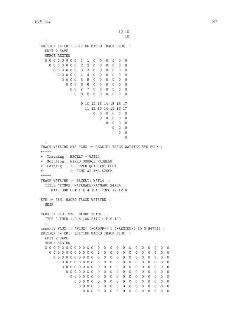
IGE–294 197

10 10

10

;


EDIT 2 SAVE

MERGE REGION

0 0 0 0 0 0 0 0 1 1 0 0 0 0 0 0

0 0 0 0 0 0 0 2 2 0 0 0 0 0 0

0 0 0 0 0 0 3 3 0 0 0 0 0 0

0 0 0 0 0 4 4 0 0 0 0 0 0

0 0 0 0 5 5 0 0 0 0 0 0

0 0 0 6 6 0 0 0 0 0 0

0 0 7 7 0 0 0 0 0 0

0 8 8 0 0 0 0 0 0

9 10 12 13 14 15 16 17

11 12 13 14 15 16 17

0 0 0 0 0 0

0 0 0 0 0

0 0 0 0

0 0 0

0 0

0

;

TRACK WATATRK SYS FLUX := DELETE: TRACK WATATRK SYS FLUX ;

*----





*----




;


SKIP

;



;



EDIT 2 SAVE

MERGE REGION

0 0 0 0 0 0 0 0 0 0 0 0 0 0 0 0 0 0 0 0 0 0 0 0

0 0 0 0 0 0 0 0 0 0 0 0 0 0 0 0 0 0 0 0 0 0 0

0 0 0 0 0 0 0 0 0 0 0 0 0 0 0 0 0 0 0 0 0 0

0 0 0 0 0 0 0 0 0 0 0 0 0 0 0 0 0 0 0 0 0

0 0 0 0 0 0 0 0 0 0 0 0 0 0 0 0 0 0 0 0

0 0 0 0 0 0 0 0 0 0 0 0 0 0 0 0 0 0 0

0 0 0 0 0 0 0 0 0 0 0 0 0 0 0 0 0 0

0 0 0 0 0 0 0 0 0 0 0 0 0 0 0 0 0

0 0 0 0 0 0 0 0 0 0 0 0 0 0 0 0

0 0 0 0 0 0 0 0 0 0 0 0 0 0 0

IGE–294 198

0 0 0 0 0 0 0 0 0 0 0 0 0 0

0 0 0 0 0 0 0 0 0 0 0 0 0

0 0 0 0 0 0 0 0 0 0 0 0

1 0 0 2 0 0 3 0 0 4 0

0 0 0 0 0 0 0 0 0 0

0 0 0 0 0 0 0 0 0

5 0 0 6 0 0 7 0

0 0 0 0 0 0 0

0 0 0 0 0 0

8 0 0 9 0

0 0 0 0

0 0 0

10 0

0

;


EDIT 2 SAVE

MERGE REGION

0 0 0 0 0 0 0 0 0 0 0 0 0 1 0 0 0 0 0 0 0 0 0 0

0 0 0 0 0 0 0 0 0 0 0 0 2 0 0 0 0 0 0 0 0 0 0

0 0 0 0 0 0 0 0 0 0 0 3 0 0 0 0 0 0 0 0 0 0

0 0 0 0 0 0 0 0 0 0 4 0 0 0 0 0 0 0 0 0 0

0 0 0 0 0 0 0 0 0 5 0 0 0 0 0 0 0 0 0 0

0 0 0 0 0 0 0 0 6 0 0 0 0 0 0 0 0 0 0

0 0 0 0 0 0 0 7 0 0 0 0 0 0 0 0 0 0

0 0 0 0 0 0 8 0 0 0 0 0 0 0 0 0 0

0 0 0 0 0 9 0 0 0 0 0 0 0 0 0 0

0 0 0 0 10 0 0 0 0 0 0 0 0 0 0

0 0 0 11 0 0 0 0 0 0 0 0 0 0

0 0 12 0 0 0 0 0 0 0 0 0 0

0 13 0 0 0 0 0 0 0 0 0 0

14 15 16 17 18 19 20 21 22 23 24

0 0 0 0 0 0 0 0 0 0

0 0 0 0 0 0 0 0 0

0 0 0 0 0 0 0 0

0 0 0 0 0 0 0

0 0 0 0 0 0

0 0 0 0 0

0 0 0 0

0 0 0

0 0

0

;

WATATRK := DELETE: WATATRK ;


END: ;

QUIT "LIST" .

6.4.4 (TCM04) – Adjuster rod in a CANDU type supercell.

This test case represents a two group calculation of incremental cross sections resulting from theinsertion of stainless steel adjuster rods in a CANDU-6 supercell.

IGE–294 199

X

Y

Z

Fuel & Sheat Adjuster

Figure 32: Geometry of the CANDU-6 supercell with stainless steel rods.


*----

* TEST CASE TCM04



* CANDU 3-D ADJUSTER ROD 1/8-ASSEMBLY

*

* REF: none

*----


*----

LINKED_LIST

BC TRACK MACRO SYS FLUX EDITION

TRACK2 SYS2 FLUX2 EDITION2 ;

SEQ_BINARY

BCTRK ;

MODULE


PROCEDURE assertS ;

*----

* Macroscopic XS

*----

MACRO := MAC: ::


READ INPUT

MIX 1 TOTAL 3.22798014E-1 3.81341100E-1

NUSIGF 5.46564534E-3 7.17375278E-2

CHI 1.0 0.0

SCAT 2 2 3.13575147E-4 3.11233580E-1

2 2 3.24143648E-1 2.19577667E-3

MIX 2 TOTAL 1.49818063E-1 1.59792125E-1

SCAT 2 2 7.40572286E-5 1.47693634E-1

2 2 1.57371104E-1 1.30506000E-3

MIX 3 TOTAL 2.60458171E-1 3.77224326E-1

IGE–294 200

SCAT 2 2 5.98954648E-5 2.49342978E-1

2 2 3.77127469E-1 1.11155845E-2

MIX 4 TOTAL 2.60458171E-1 3.77224326E-1

SCAT 2 2 5.98954648E-5 2.49342978E-1

2 2 3.77127469E-1 1.11155845E-2

;

*----

* Geometry : BC - 3D Cartesian assembly with annular regions

* Tracking : 1) EXCELT ALLG

* 2) EXCELT XCLL

*----

BC := GEO: :: CAR3D 3 2 2

X- REFL X+ SYME Y- REFL Y+ SYME Z- REFL Z+ SYME

CELL M MX MX MX FXY MXY M MX BX MX FXY BXY

TURN A A A F A A A A A F A A

::: M := GEO: CAR3D 1 1 1

MESHX 0.0 7.14375 MESHY 0.0 7.14375 MESHZ -8.25500 +8.25500

SPLITZ 2 MIX 3

;

::: MX := GEO: M

MESHX -7.14375 +7.14375 SPLITX 2

;

::: MXY := GEO: MX

MESHY -7.14375 +7.14375 SPLITY 2

;

::: BX := GEO: CARCELY 2 1

MESHX -7.14375 +7.14375 SPLITX 2

MESHY 0.0 +7.14375

MESHZ -8.25500 +8.25500 SPLITZ 2

RADIUS 0.0 3.5100 3.8100

MIX 3 4 3

;

::: BXY := GEO: BX

MESHY -7.14375 +7.14375 SPLITY 2

;

::: FXY := GEO: CARCELZ 2 1

MESHX -7.14375 +7.14375 SPLITX 2

MESHY -7.14375 +7.14375 SPLITY 2

MESHZ -8.25500 +8.25500 SPLITZ 2

RADIUS 0.0 5.16890 6.58750

MIX 1 2 3

;

;

TRACK BCTRK := EXCELT: BC ::

TITLE ’TCM04: TWO GROUPS CANDU 3-D ADJUSTER ROD ASSEMBLY ’

MAXR 40 ALLG TRAK TISO 4 2.5

;

SYS := ASM: MACRO TRACK BCTRK ;

TRACK2 := EXCELT: BC ::

TITLE ’TCM04: TWO GROUPS CANDU 3-D ADJUSTER ROD ASSEMBLY ’

MAXR 40 XCLL TRAK TISO 4 2.5

;

SYS2 := ASM: MACRO TRACK2 ;

*----

IGE–294 201

* Solution : K-EFFECTIVE

* Editing : Compute reference reaction rates

*----


TYPE K

;

assertS FLUX :: ’K-EFFECTIVE’ 1 1.103927 ;


EDIT 3 UPS MERG COMP SAVE ON ’NOROD’

;

FLUX := FLU: FLUX SYS2 MACRO TRACK2 ::

TYPE K

;


EDITION := EDI: EDITION MACRO TRACK2 FLUX ::

EDIT 3 UPS MERG COMP STAT ALL REFE ’NOROD’

;

EDITION2 := EDI: MACRO TRACK2 FLUX ::

EDIT 3 UPS MERG COMP SAVE ON ’NOROD’

;

SYS SYS2 := DELETE: SYS SYS2 ;

*----

* Modify Macrolib for adjuster rod material

* Solution : K-EFFECTIVE

* Editing : Compute Delta-Sigma

*----

MACRO := MAC: MACRO ::

READ INPUT

MIX 4 TOTAL 6.96358740E-1 1.12379551E+0

SCAT 2 2 2.55611958E-4 6.77430272E-1

2 2 9.55488145E-1 3.16311372E-3

;

SYS := ASM: MACRO TRACK BCTRK ;

SYS2 := ASM: MACRO TRACK2 ;


TYPE K

;



EDIT 3 UPS MERG COMP STAT DELS REFE ’NOROD’

;

FLUX := FLU: FLUX SYS2 MACRO TRACK2 ::

TYPE K

;


EDITION2 := EDI: EDITION2 MACRO TRACK2 FLUX ::

EDIT 3 UPS MERG COMP STAT DELS REFE ’NOROD’

;

BCTRK := DELETE: BCTRK ;


END: ;

QUIT "LIST" .

IGE–294 202

6.4.5 (TCM05) – Comparison of leakage models

This test presents various homogeneous and heterogeneous leakage models on a simple cell.


*----

* TEST CASE TCM05



* 2-D CARTESIAN/ANNULAR CELL

* Validating leakage options

* TYPE K B L FOR MOSTELC (NO VOID)

* TYPE K B L FOR MOSTELCV (MOSTELC WITH VOID)

*

*----


*----

LINKED_LIST

MOSTELC MOSTELCV TRACK MACRO SYS FLUX EDITION ;

SEQ_BINARY

TRKSPC ;

MODULE


PROCEDURE assertS ;

*----

* Macroscopic XS

*----

MACRO := MAC: ::

NGRO 2 ANIS 2 NMIX 2 NIFI 1

READ INPUT

MIX 1 TOTAL 0.222222 0.833333

SCAT 1 1 0.19222 2 2 0.75333 0.02

1 1 0.1 2 2 0.5 0.01

NUSIGF 0.0 0.135 CHI 1.0 0.0

MIX 2 TOTAL 0.166667 1.111111

SCAT 2 2 0.00015 0.126667 2 2 1.10111 0.04

2 2 0.0001 0.1 2 2 0.5 0.01

;

*----

* Geometry : MOSTELC - Cartesian 2D cell without void region

* MOSTELCV - Cartesian 2D cell with void region

*----


X- REFL X+ REFL Y- REFL Y+ REFL

MESHX 0.0 1.26209 MESHY 0.0 1.26209

RADIUS 0.0 0.39306 0.45802 SPLITR 2 1

MIX 1 2 2 ;

MOSTELCV := GEO: MOSTELC ::

MIX 1 0 2 ;

*----

* Tracking : EXCELT - MOSTELC

* ANIS 2 for adequate dimensions in PIJK

* Solution : TYPE K, B or L

* Leakage : B1 PNL, B1 HETE

IGE–294 203

*----

TRACK TRKSPC := EXCELT: MOSTELC ::

TITLE ’TCM05: ANNULAR GEOMETRY WITH MACROSCOPIC XS’

MAXR 5 ANIS 2 TRAK TISO 12 20.0 ;

SYS := ASM: MACRO TRACK TRKSPC ::

PIJK ;


TYPE K ;

assertS FLUX :: ’K-INFINITY’ 1 1.199508 ;


EDIT 2 SAVE ;


TYPE K B1 PNL BUCK 1.51429E-03 ;



EDIT 2 SAVE ;


TYPE B B1 PNL KEFF 1.199538 ;



EDIT 2 SAVE ;


TYPE B B1 PNL ;



EDIT 2 SAVE ;


TYPE L B1 PNL ;



EDIT 2 SAVE ;

FLUX := DELETE: FLUX ;


TYPE K B1 HETE BUCK 1.50298E-03 ;



EDIT 2 SAVE ;


TYPE B B1 HETE KEFF 1.199538 ;



EDIT 2 SAVE ;


TYPE B B1 HETE R BUCK Z 5.00993E-04 ;



EDIT 2 SAVE ;


TYPE B B1 HETE Z BUCK R 1.001986E-03 ;



EDIT 2 SAVE ;


TYPE B B1 HETE ;


IGE–294 204


EDIT 2 SAVE ;


TYPE L B1 HETE R BUCK Z 5.00993E-04 ;



EDIT 2 SAVE ;


TYPE L B1 HETE Z BUCK R 1.001986E-03 ;



EDIT 2 SAVE ;


TYPE L B1 HETE ;



EDIT 2 SAVE ;

FLUX SYS := DELETE: FLUX SYS ;

*----

* Tracking : EXCELT - MOSTELCV only update TRACK TRKSPC files

* since only change is in one material

* Solution : TYPE K, B or L

* Leakage : B1 PNL, B1 HETE

*----

TRACK TRKSPC := EXCELT: TRACK TRKSPC MOSTELCV ::

TITLE ’TCM05: ANNULAR GEOMETRY WITH MACROSCOPIC XS (VOID)’ ;

SYS := ASM: MACRO TRACK TRKSPC ::

PIJK ;


TYPE K ;



EDIT 2 SAVE ;





EDIT 2 SAVE ;


TYPE B B1 PNL KEFF 1.228007 ;



EDIT 2 SAVE ;


TYPE B B1 PNL ;



EDIT 2 SAVE ;


TYPE L B1 PNL ;



EDIT 2 SAVE ;



IGE–294 205

TYPE K B1 HETE BUCK 1.40181E-03 ;



EDIT 2 SAVE ;


TYPE B B1 HETE KEFF 1.228007 ;



EDIT 2 SAVE ;


TYPE B B1 HETE R BUCK Z 5.00993E-04 ;



EDIT 2 SAVE ;


TYPE B B1 HETE Z BUCK R 1.001986E-03 ;



EDIT 2 SAVE ;


TYPE B B1 HETE ;



EDIT 2 SAVE ;


TYPE L B1 HETE R BUCK Z 5.00993E-04 ;



EDIT 2 SAVE ;


TYPE L B1 HETE Z BUCK R 1.001986E-03 ;



EDIT 2 SAVE ;


TYPE L B1 HETE ;



EDIT 2 SAVE ;

TRKSPC := DELETE: TRKSPC ;


END: ;

QUIT "LIST" .

6.4.6 (TCM06) – Buckling search without fission source

This test is for an homogeneous water cell. A buckling eigenvalue problem is solved in the abscenceof fission source for the neutron flux distribution inside this cell.


*----

* TEST CASE TCM06


IGE–294 206

* BUCKLING SEARCH PROBLEM WITHOUT FISSION SOURCE

* HOMOGENEOUS GEOMETRY

*

* REF: none

*----


*----

LINKED_LIST

WATER TRACK MACRO SYS FLUX EDITION ;

MODULE

GEO: SYBILT: MAC: ASM: FLU: EDI: END: ;

PROCEDURE assertS ;

*----

* Macroscopic XS

*----

MACRO := MAC: ::

EDIT 2 NGRO 1 ANIS 2 NMIX 1 NIFI 0

READ INPUT

MIX 1 TOTAL 3.59 SCAT 1 1 3.57 1 1 2.38

;

*----

* Geometry : WATER - Homogeneous geometry

* Tracking : SYBILT

*----

WATER := GEO: :: HOMOGE

MIX 1

;

TRACK := SYBILT: WATER ::

TITLE ’TCM06: ENE6101 EXAM’

MAXR 1

;

*----

* Solution : TYPE L

* Leakage : B0 PNL, P0 PNL, B1 PNL, P1 PNL

*----

SYS := ASM: MACRO TRACK ;


TYPE L B0 SIGS EXTE 5 1.0E-5 BUCK -0.07 ;

assertS FLUX :: ’B2 B1HOM’ 1 -2.14440E-01 ;


EDIT 3 SAVE ;


TYPE L P0 SIGS EXTE 5 1.0E-5 BUCK -0.07 ;



EDIT 3 SAVE ;


TYPE L B1 SIGS EXTE 5 1.0E-5 BUCK -0.07 ;



EDIT 3 SAVE ;


TYPE L P1 SIGS EXTE 5 1.0E-5 BUCK -0.07 ;



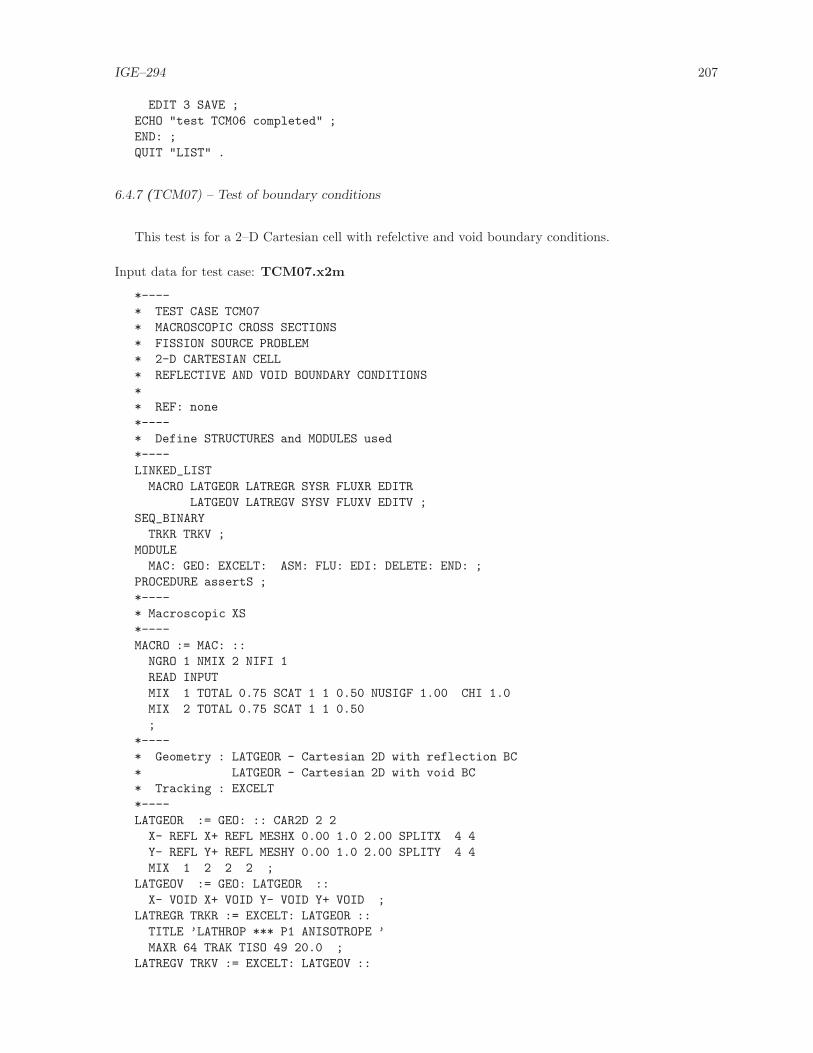
IGE–294 207

EDIT 3 SAVE ;


END: ;

QUIT "LIST" .

6.4.7 (TCM07) – Test of boundary conditions

This test is for a 2–D Cartesian cell with refelctive and void boundary conditions.


*----

* TEST CASE TCM07



* 2-D CARTESIAN CELL

* REFLECTIVE AND VOID BOUNDARY CONDITIONS

*

* REF: none

*----


*----

LINKED_LIST

MACRO LATGEOR LATREGR SYSR FLUXR EDITR

LATGEOV LATREGV SYSV FLUXV EDITV ;

SEQ_BINARY

TRKR TRKV ;

MODULE

MAC: GEO: EXCELT: ASM: FLU: EDI: DELETE: END: ;

PROCEDURE assertS ;

*----

* Macroscopic XS

*----

MACRO := MAC: ::


READ INPUT

MIX 1 TOTAL 0.75 SCAT 1 1 0.50 NUSIGF 1.00 CHI 1.0


;

*----

* Geometry : LATGEOR - Cartesian 2D with reflection BC

* LATGEOR - Cartesian 2D with void BC

* Tracking : EXCELT

*----

LATGEOR := GEO: :: CAR2D 2 2

X- REFL X+ REFL MESHX 0.00 1.0 2.00 SPLITX 4 4

Y- REFL Y+ REFL MESHY 0.00 1.0 2.00 SPLITY 4 4

MIX 1 2 2 2 ;

LATGEOV := GEO: LATGEOR ::

X- VOID X+ VOID Y- VOID Y+ VOID ;

LATREGR TRKR := EXCELT: LATGEOR ::

TITLE ’LATHROP *** P1 ANISOTROPE ’


LATREGV TRKV := EXCELT: LATGEOV ::

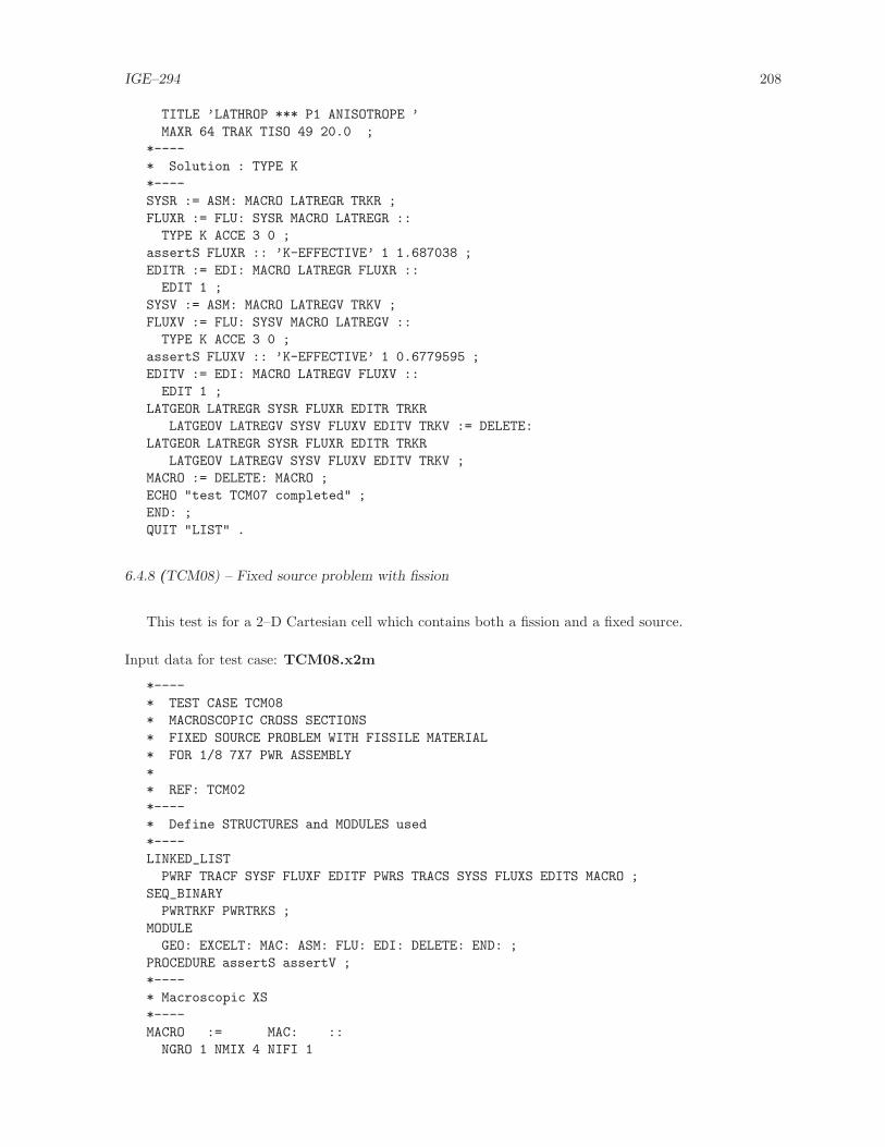
IGE–294 208

TITLE ’LATHROP *** P1 ANISOTROPE ’


*----

* Solution : TYPE K

*----

SYSR := ASM: MACRO LATREGR TRKR ;

FLUXR := FLU: SYSR MACRO LATREGR ::

TYPE K ACCE 3 0 ;

assertS FLUXR :: ’K-EFFECTIVE’ 1 1.687038 ;

EDITR := EDI: MACRO LATREGR FLUXR ::

EDIT 1 ;

SYSV := ASM: MACRO LATREGV TRKV ;

FLUXV := FLU: SYSV MACRO LATREGV ::

TYPE K ACCE 3 0 ;

assertS FLUXV :: ’K-EFFECTIVE’ 1 0.6779595 ;

EDITV := EDI: MACRO LATREGV FLUXV ::

EDIT 1 ;

LATGEOR LATREGR SYSR FLUXR EDITR TRKR

LATGEOV LATREGV SYSV FLUXV EDITV TRKV := DELETE:

LATGEOR LATREGR SYSR FLUXR EDITR TRKR

LATGEOV LATREGV SYSV FLUXV EDITV TRKV ;

MACRO := DELETE: MACRO ;


END: ;

QUIT "LIST" .

6.4.8 (TCM08) – Fixed source problem with fission

This test is for a 2–D Cartesian cell which contains both a fission and a fixed source.


*----

* TEST CASE TCM08


* FIXED SOURCE PROBLEM WITH FISSILE MATERIAL

* FOR 1/8 7X7 PWR ASSEMBLY

*

* REF: TCM02

*----


*----

LINKED_LIST

PWRF TRACF SYSF FLUXF EDITF PWRS TRACS SYSS FLUXS EDITS MACRO ;

SEQ_BINARY

PWRTRKF PWRTRKS ;

MODULE


PROCEDURE assertS assertV ;

*----

* Macroscopic XS

*----

MACRO := MAC: ::


IGE–294 209

READ INPUT

MIX 1 TOTAL 1.250 SCAT 1 1 1.242

NUSIGF 0.15 CHI 1.0

MIX 2 TOTAL 0.625 SCAT 1 1 0.355

FIXE 0.000

MIX 3 TOTAL 14.000 SCAT 1 1 0.000

FIXE 1.000

MIX 4 TOTAL 1.250 SCAT 1 1 1.242

FIXE 0.000

;

*----

* Geometry : PWRF - Cartesian 2D assembly with fission

* PWRS - Cartesian 2D assembly without fission

* Tracking : EXCELT

*----

PWRF := GEO: :: CAR2D 4 4


CELL P F F F

F F F

F F

F


RADIUS 0.000 0.450

MIX 2 1


MESHY -0.625 0.625 SPLITY 2 ;

::: P := GEO: F

MIX 3 1

SPLITR 3 ;

;

PWRS := GEO: :: CAR2D 4 4


CELL P F F F

F F F

F F

F


RADIUS 0.000 0.450

MIX 2 4


MESHY -0.625 0.625 SPLITY 2 ;

::: P := GEO: F

MIX 3 4

SPLITR 3 ;

;

TRACF PWRTRKF := EXCELT: PWRF ::



SYSF := ASM: MACRO TRACF PWRTRKF ;

TRACS PWRTRKS := EXCELT: PWRS ::



SYSS := ASM: MACRO TRACS PWRTRKS ;

*----

* Solution : TYPE K to test if k < 1.0

IGE–294 210

* TYPE S to include fixed source

*----

FLUXF := FLU: SYSF MACRO TRACF ::

TYPE K ;

assertS FLUXF :: ’K-EFFECTIVE’ 1 0.8165358 ;

EDITF := EDI: MACRO TRACF FLUXF ::

EDIT 2 SAVE

MERGE REGION

1 1 1 2 3 4 3 4 5 6 5 6 7 8 7 8

9 10 9 10 9 10 11 12 11 12 11 12 11 12 13 14 13 14 13 14 13 14

15 16 15 16 15 16 17 18 17 18 17 18 17 18

19 20 19 20 19 20 ;

EDITF := DELETE: EDITF ;

*----

* SINCE KEFF < 1 DO FIXED SOURCE PROBLEM

* (FIXED AND FISSION SOURCES TAKEN INTO ACCOUNT)

*----

FLUXF := FLU: FLUXF SYSF MACRO TRACF ::

TYPE S ;

EDITF := EDI: MACRO TRACF FLUXF ::

EDIT 2 SAVE

MERGE REGION

1 1 1 2 3 4 3 4 5 6 5 6 7 8 7 8

9 10 9 10 9 10 11 12 11 12 11 12 11 12 13 14 13 14 13 14 13 14

15 16 15 16 15 16 17 18 17 18 17 18 17 18

19 20 19 20 19 20 ;

*----

* Solution : TYPE S only since no fission

*----

*

* IF KEFF < 1 DO FIXED SOURCE PROBLEM PROBLEM

* (FIXED AND FISSION SOURCES TAKEN INTO ACCOUNT)

*

FLUXS := FLU: SYSS MACRO TRACS ::

TYPE S ;

assertV FLUXS :: ’FLUX’ (*GROUP*) 1 (*REGION*) 10 6.728200E-03 ;

EDITS := EDI: MACRO TRACS FLUXS ::

EDIT 2 SAVE

MERGE REGION

1 1 1 2 3 4 3 4 5 6 5 6 7 8 7 8

9 10 9 10 9 10 11 12 11 12 11 12 11 12 13 14 13 14 13 14 13 14

15 16 15 16 15 16 17 18 17 18 17 18 17 18

19 20 19 20 19 20 ;

PWRTRKS PWRTRKF := DELETE: PWRTRKS PWRTRKF ;


END: ;

QUIT "LIST" .

6.4.9 (TCM09) – Solution of a 2-D fission source problem using MCCGT:

This test case is for a 3×3 Cartesian assembly in 2-D similar to TCM03. It is solved using the methodof cyclic characteristics.

IGE–294 211


*----

* TEST CASE TCM09




* WATANABE-MAYNARD PROBLEM SIMILAR TO TCM09

*

* REF: R. Roy, "The Cyclic Characteristics Method,"

* Int. Conf. Physics of Nuclear Science and Technology,

* Long Island, NY, October 1998, pp. 407-414.

*----

*

LINKED_LIST WATA WAT24 TRACK MACRO SYS FLUX EDITION ;

SEQ_BINARY WATATRK ;

STRING PolarAng := "CACB" ;

MODULE GEO: EXCELT: MCCGT: MAC: ASM: FLU: EDI: DELETE: END: ;

PROCEDURE assertV ;

*


MACRO := MAC: ::

NGRO 1 NMIX 3

READ INPUT



MIX 3 TOTAL 0.0 SCAT 1 1 0.00 ;

* GEOMETRIES ENTERED WITH SYMMETRIES


WATA := GEO: :: CAR2D 3 3

X- DIAG X+ VOID

MESHX 0.00 1.25 5.00 10.00

Y- REFL Y+ DIAG

MESHY 0.00 1.25 5.00 10.00

MIX 1 3 2

3 2

2 ;


SPLITX 3 9 12

SPLITY 3 9 12 ;

* SOLUTION FOR WAT24



MAXR 300

TRAK TSPC 12 12.0 ;

TRACK := MCCGT: TRACK WATATRK ::

EDIT 1 <<PolarAng>> 4

AAC 80 TMT EPSI 1E-5 MCU 2500

MAXI 1 KRYL 0 SCR 0 HDD 0.0 ;


EDIT 2 ARM ;

FLUX := FLU: MACRO TRACK SYS WATATRK ::

TYPE S THER 1.E-6 100 EXTE 1.E-6 100 ;

* UPPER QUADRANT FLUX FOR 24X24

* RESULTS GIVEN IN TABLE 1. (ref. p. 411 )

EDITION := EDI: FLUX MACRO TRACK ::

IGE–294 212

EDIT 2 SAVE

MERGE REGION

0 0 0 0 0 0 0 0 0 0 0 0 0 0 0 0 0 0 0 0 0 0 0 0

0 0 0 0 0 0 0 0 0 0 0 0 0 0 0 0 0 0 0 0 0 0 0

0 0 0 0 0 0 0 0 0 0 0 0 0 0 0 0 0 0 0 0 0 0

0 0 0 0 0 0 0 0 0 0 0 0 0 0 0 0 0 0 0 0 0

0 0 0 0 0 0 0 0 0 0 0 0 0 0 0 0 0 0 0 0

0 0 0 0 0 0 0 0 0 0 0 0 0 0 0 0 0 0 0

0 0 0 0 0 0 0 0 0 0 0 0 0 0 0 0 0 0

0 0 0 0 0 0 0 0 0 0 0 0 0 0 0 0 0

0 0 0 0 0 0 0 0 0 0 0 0 0 0 0 0

0 0 0 0 0 0 0 0 0 0 0 0 0 0 0

0 0 0 0 0 0 0 0 0 0 0 0 0 0

0 0 0 0 0 0 0 0 0 0 0 0 0

0 0 0 0 0 0 0 0 0 0 0 0

1 0 0 2 0 0 3 0 0 4 0

0 0 0 0 0 0 0 0 0 0

0 0 0 0 0 0 0 0 0

5 0 0 6 0 0 7 0

0 0 0 0 0 0 0

0 0 0 0 0 0

8 0 0 9 0

0 0 0 0

0 0 0

10 0

0

;

* FLUX AT X=5.625CM FOR 24X24

EDITION := EDI: EDITION FLUX MACRO TRACK ::

EDIT 2 SAVE

MERGE REGION

0 0 0 0 0 0 0 0 0 0 0 0 0 1 0 0 0 0 0 0 0 0 0 0

0 0 0 0 0 0 0 0 0 0 0 0 2 0 0 0 0 0 0 0 0 0 0

0 0 0 0 0 0 0 0 0 0 0 3 0 0 0 0 0 0 0 0 0 0

0 0 0 0 0 0 0 0 0 0 4 0 0 0 0 0 0 0 0 0 0

0 0 0 0 0 0 0 0 0 5 0 0 0 0 0 0 0 0 0 0

0 0 0 0 0 0 0 0 6 0 0 0 0 0 0 0 0 0 0

0 0 0 0 0 0 0 7 0 0 0 0 0 0 0 0 0 0

0 0 0 0 0 0 8 0 0 0 0 0 0 0 0 0 0

0 0 0 0 0 9 0 0 0 0 0 0 0 0 0 0

0 0 0 0 10 0 0 0 0 0 0 0 0 0 0

0 0 0 11 0 0 0 0 0 0 0 0 0 0

0 0 12 0 0 0 0 0 0 0 0 0 0

0 13 0 0 0 0 0 0 0 0 0 0

14 15 16 17 18 19 20 21 22 23 24

0 0 0 0 0 0 0 0 0 0

0 0 0 0 0 0 0 0 0

0 0 0 0 0 0 0 0

0 0 0 0 0 0 0

0 0 0 0 0 0

0 0 0 0 0

0 0 0 0

0 0 0

IGE–294 213

0 0

0

;

WATATRK := DELETE: WATATRK ;



END: ;

QUIT "LIST" .

6.4.10 (TCM10) – Solution of a 2-D fixed source problem using MCCGT:

This test case is for a 2–D Cartesian assembly that contains a fixed source. It is solved using themethod of cyclic characteristics.


*

* TEST CASE TCM10




* TSAI-LOYALKA SEMI-INFINITE PROBLEM

*




*

LINKED_LIST LOYA LOY25 TRACK FLUX EDITION

MACRO SYS MACRO100 MACRO050 MACRO010 MACRO005 MACRO000 ;

SEQ_BINARY LOYATRK ;

STRING PolarAng := "CACB" ;

MODULE GEO: EXCELT: MCCGT: MAC: ASM: FLU: EDI: DELETE: END: ;

PROCEDURE assertV ;

INTEGER i n := 1 1 ;

*


MACRO100 := MAC: ::

NGRO 1 NMIX 2

READ INPUT


MIX 2 TOTAL 1.0 SCAT 1 1 1.00 ;

MACRO050 := MAC: ::

NGRO 1 NMIX 2

READ INPUT


MIX 2 TOTAL 1.0 SCAT 1 1 0.50 ;

MACRO010 := MAC: ::

NGRO 1 NMIX 2

READ INPUT


MIX 2 TOTAL 1.0 SCAT 1 1 0.10 ;

MACRO005 := MAC: ::

NGRO 1 NMIX 2

READ INPUT

IGE–294 214


MIX 2 TOTAL 1.0 SCAT 1 1 0.05 ;

MACRO000 := MAC: ::

NGRO 1 NMIX 2

READ INPUT


MIX 2 TOTAL 1.0 SCAT 1 1 0.00 ;

* GEOMETRIES ENTERED WITH SYMMETRIES

* LOYA - 2 X 2 REGIONS

* LOY25 - 25 X 25 REGIONS

LOYA := GEO: :: CAR2D 2 2

X- REFL X+ VOID

MESHX 0.00 0.52 1.00

Y- REFL Y+ REFL

MESHY 0.00 0.52 1.00

MIX 1 2

2 2 ;

LOY25 := GEO: LOYA ::

SPLITX 13 12

SPLITY 13 12 ;

* SOLUTION FOR LOY25

TRACK LOYATRK := EXCELT: LOY25 ::

TITLE ’TCM10: LOYANABE-MAYNARD 24X24 ’

MAXR 625

TRAK TSPC 12 100.0 ;

TRACK := MCCGT: TRACK LOYATRK ::

EDIT 1 <<PolarAng>> 2

AAC 1 TMT SCR 0 EPSI 1E-5

MAXI 100 KRYL 30 HDD 0.0 ;

REPEAT

IF i 1 = THEN

MACRO := MACRO100 ;

ELSEIF i 2 = THEN

MACRO := MACRO050 ;

ELSEIF i 3 = THEN

MACRO := MACRO010 ;

ELSEIF i 4 = THEN

MACRO := MACRO005 ;

ELSEIF i 5 = THEN

MACRO := MACRO000 ;

ENDIF ;

SYS := ASM: MACRO TRACK LOYATRK ::

EDIT 2 ARM ;

FLUX := FLU: MACRO TRACK SYS LOYATRK ::

TYPE S ;

* SOLUTION FOR LOY25

* FLUX AT X=Y= 0.50, 0.70 AND 0.98

* SEE TABLE 2. (ref. p. 412)


EDIT 2 SAVE

MERGE REGION

0 0 0 0 0 0 0 0 0 0 0 0 0 0 0 0 0 0 0 0 0 0 0 0 0

0 0 0 0 0 0 0 0 0 0 0 0 0 0 0 0 0 0 0 0 0 0 0 0 0

0 0 0 0 0 0 0 0 0 0 0 0 0 0 0 0 0 0 0 0 0 0 0 0 0

0 0 0 0 0 0 0 0 0 0 0 0 0 0 0 0 0 0 0 0 0 0 0 0 0

IGE–294 215

0 0 0 0 0 0 0 0 0 0 0 0 0 0 0 0 0 0 0 0 0 0 0 0 0

0 0 0 0 0 0 0 0 0 0 0 0 0 0 0 0 0 0 0 0 0 0 0 0 0

0 0 0 0 0 0 0 0 0 0 0 0 0 0 0 0 0 0 0 0 0 0 0 0 0

0 0 0 0 0 0 0 0 0 0 0 0 0 0 0 0 0 0 0 0 0 0 0 0 0

0 0 0 0 0 0 0 0 0 0 0 0 0 0 0 0 0 0 0 0 0 0 0 0 0

0 0 0 0 0 0 0 0 0 0 0 0 0 0 0 0 0 0 0 0 0 0 0 0 0

0 0 0 0 0 0 0 0 0 0 0 0 0 0 0 0 0 0 0 0 0 0 0 0 0

0 0 0 0 0 0 0 0 0 0 0 0 0 0 0 0 0 0 0 0 0 0 0 0 0

0 0 0 0 0 0 0 0 0 0 0 0 1 0 0 0 0 0 0 0 0 0 0 0 0

0 0 0 0 0 0 0 0 0 0 0 0 0 0 0 0 0 0 0 0 0 0 0 0 0

0 0 0 0 0 0 0 0 0 0 0 0 0 0 0 0 0 0 0 0 0 0 0 0 0

0 0 0 0 0 0 0 0 0 0 0 0 0 0 0 0 0 0 0 0 0 0 0 0 0

0 0 0 0 0 0 0 0 0 0 0 0 0 0 0 0 0 0 0 0 0 0 0 0 0

0 0 0 0 0 0 0 0 0 0 0 0 0 0 0 0 0 2 0 0 0 0 0 0 0

0 0 0 0 0 0 0 0 0 0 0 0 0 0 0 0 0 0 0 0 0 0 0 0 0

0 0 0 0 0 0 0 0 0 0 0 0 0 0 0 0 0 0 0 0 0 0 0 0 0

0 0 0 0 0 0 0 0 0 0 0 0 0 0 0 0 0 0 0 0 0 0 0 0 0

0 0 0 0 0 0 0 0 0 0 0 0 0 0 0 0 0 0 0 0 0 0 0 0 0

0 0 0 0 0 0 0 0 0 0 0 0 0 0 0 0 0 0 0 0 0 0 0 0 0

0 0 0 0 0 0 0 0 0 0 0 0 0 0 0 0 0 0 0 0 0 0 0 0 0

0 0 0 0 0 0 0 0 0 0 0 0 0 0 0 0 0 0 0 0 0 0 0 0 3

;

IF i 1 = THEN


ELSEIF i 2 = THEN


ELSEIF i 3 = THEN


ELSEIF i 4 = THEN


ELSEIF i 5 = THEN


ENDIF ;

SYS FLUX MACRO EDITION := DELETE: SYS FLUX MACRO EDITION ;

EVALUATE i := i 1 + ;

UNTIL i 6 = ;

LOYATRK := DELETE: LOYATRK ;


END: ;

QUIT "LIST" .

6.4.11 (TCM11) – Comparison of CP and MoC solutions

This test case is for a 4 × 4 Cartesian assembly in 2-D. It is solved using the method of cycliccharacteristics and the method of collision probabilities using specular (mirror like) boundary conditions.

IGE–294 216


*

* TEST CASE TCM11



* CARTESIAN 4 X 4 ASSEMBLY WITH FUEL RODS AND POISON

* KAVENOKY BENCHMARK

*




*

STRING Polar_Ang := "CACB" ;

INTEGER Nazimuth := 8 ;

REAL DenTrak := 100. ;

INTEGER Nsplit := 5 ;

REAL Tolerance := 5.E-6 ;

LINKED_LIST PWR TRACK MACRO SYS FLUX EDITION ;

SEQ_BINARY PWRTRK ;

MODULE GEO: EXCELT: MCCGT: MAC: ASM: FLU: EDI: END: DELETE: GREP: ;

PROCEDURE assertV ;

REAL ou := 100. ;

REAL

f1 f2 f3 f8 f9 f10 f11 f12 f13 f14 f15

v1 v2 v3 v8 v9 v10 v11 v12 v13 v14 v15 ;

REAL

r1 r2 r3

r8 r9 r10

r11 r12 r13 r14 r15 :=

5.166 3.699 4.183

3.178 3.617 0.2847

2.913 3.441 3.937 3.225 3.673 ;

REAL

e1 e2 e3

e8 e9 e10

e11 e12 e13 e14 e15 :=

0.11 0.08 0.07

0.04 0.05 0.002

0.03 0.03 0.04 0.05 0.05 ;

EVALUATE

e1 e2 e3

e8 e9 e10

e11 e12 e13 e14 e15 :=

e1 r1 / e2 r2 / e3 r3 /

e8 r8 / e9 r9 / e10 r10 /

e11 r11 / e12 r12 / e13 r13 / e14 r14 / e15 r15 / ;

EVALUATE

e1 e2 e3

e8 e9 e10

e11 e12 e13 e14 e15 :=

e1 ou * e2 ou * e3 ou *

e8 ou * e9 ou * e10 ou *

e11 ou * e12 ou * e13 ou * e14 ou * e15 ou * ;

*----

* Macroscopic XS

IGE–294 217

*----

MACRO := MAC: ::

NGRO 1 NMIX 19

READ INPUT




















;

*----

* Geometry : PWR - Cartesian 7x7

* Tracking : EXCELT

*----

PWR := GEO: :: CAR2D 4 4


CELL WA F2 F4 F6

F8 P10 F12

F14 F16

F18

::: WA := GEO: CAR2D 1 1

MESHX -0.625 0.625 SPLITX <<Nsplit>>

MESHY -0.625 0.625 SPLITY <<Nsplit>>

MIX 1 ;

::: F2 := GEO: CARCEL 1

MESHX -0.625 0.625 SPLITX <<Nsplit>>

MESHY -0.625 0.625 SPLITY <<Nsplit>>

RADIUS 0.000 0.450

MIX 2 3 ;

::: F4 := GEO: F2

MIX 4 5 ;

::: F6 := GEO: F2

MIX 6 7 ;

::: F8 := GEO: F2

MIX 8 9 ;

::: P10 := GEO: F2

MIX 10 11 SPLITR 3 ;

::: F12 := GEO: F2

MIX 12 13 ;

::: F14 := GEO: F2

MIX 14 15 ;

IGE–294 218

::: F16 := GEO: F2

MIX 16 17 ;

::: F18 := GEO: F2

MIX 18 19 ;

;

TRACK PWRTRK := EXCELT: PWR ::

MAXR 300 TRAK TSPC <<Nazimuth>> <<DenTrak>> ;

TRACK := MCCGT: TRACK PWRTRK ::

EDIT 1 <<Polar_Ang>> 4

AAC 80 TMT EPSI 1E-5

MAXI 1 KRYL 0 SCR 0 HDD 0.0 ;

SYS := ASM: MACRO TRACK PWRTRK ::

EDIT 2 ARM ;

FLUX := FLU: MACRO TRACK SYS PWRTRK ::

TYPE S

THER <<Tolerance>> 100 EXTE <<Tolerance>> 100 ;


EDIT 2 SAVE

MERGE MIX 1 2 3 0 0 0 0 4 5 6 7 8 9 10 11 0 0 0 0 ;

GREP: EDITION ::

STEP UP ’REF-CASE0001’ STEP UP MACROLIB

GETVAL VOLUME 1 11

>>v1<< >>v2<< >>v3<< >>v8<< >>v9<< >>v10<<

>>v11<< >>v12<< >>v13<< >>v14<< >>v15<<

STEP UP ’GROUP’ STEP AT 1

GETVAL FLUX-INTG 1 11

>>f1<< >>f2<< >>f3<< >>f8<< >>f9<< >>f10<<

>>f11<< >>f12<< >>f13<< >>f14<< >>f15<<

;

EVALUATE f1 f2 f3 f8 f9 f10 f11 f12 f13 f14 f15 :=

f1 v1 / r1 - r1 / ou *

f2 v2 / r2 - r2 / ou *

f3 v3 / r3 - r3 / ou *

f8 v8 / r8 - r8 / ou *

f9 v9 / r9 - r9 / ou *

f10 v10 / r10 - r10 / ou *

f11 v11 / r11 - r11 / ou *

f12 v12 / r12 - r12 / ou *

f13 v13 / r13 - r13 / ou *

f14 v14 / r14 - r14 / ou *

f15 v15 / r15 - r15 / ou *

;

* SOLUTION FOR KAVENORY BENCHMARK

* FLUX VALUES COMPARED TO MONTE-CARLO RESULTS

* SEE TABLE 3. (ref. p. 412)

ECHO "DF( 1/ 3)%=" f1 f2 f3 ;

ECHO "DF( 8/ 9)%=" f8 f9 ;

ECHO "DF(10/12)%=" f10 f11 f12 ;

ECHO "DF(13/15)%=" f13 f14 f15 ;

ECHO "ACCEPT=" f1 ABS e1 <= f2 ABS e2 <= f3 ABS e3 <= ;

ECHO "ACCEPT=" f8 ABS e8 <= f9 ABS e9 <= ;



PWRTRK := DELETE: PWRTRK ;


IGE–294 219


END: ;

QUIT .

6.4.12 (TCM12) - Solution of a 3-D problem using the MCU: module

This test case is for a simplified 3-D Cartesian assembly analyzed using the EXCELT:. A collisionsprobability solution is generated as well as two solutions using the method of characteristics.


*

* TEST CASE TCM12



* 3D HEXAGONAL S30 ASSEMBLY WITH FUEL RODS

*

LINKED_LIST GEOMETRY TRACKING ASSEMBLY MACLIB FLUX ;

MODULE MAC: GEO: EXCELT: ASM: FLU: TRIVAT: END: ;

SEQ_BINARY TRKSPC ;

PROCEDURE assertS ;

MACLIB := MAC: ::

EDIT 2 NGRO 1 NMIX 4 NIFI 1

READ INPUT

MIX 1

TOTAL 0.41 SCAT 1 1 0.3

NUSIGF 0.1 CHI 1.0

MIX 2

TOTAL 0.53 SCAT 1 1 0.5

MIX 3

TOTAL 0.45 SCAT 1 1 0.347

NUSIGF 0.17 CHI 1.0

MIX 4

TOTAL 0.3 SCAT 1 1 0.2

NUSIGF 0.1 CHI 1.0

;

GEOMETRY := GEO: :: HEXZ 2 2

EDIT 2

HBC S30 REFL Z+ REFL Z- REFL

MIX UDEPLETED_1 UDEPLETED_1 UDEPLETED_2 UDEPLETED_2

::: UDEPLETED_1 := GEO: HEXCELZ 4 1

EDIT 2

SIDE 2.804

RADIUS 0.0 2.23 2.275 2.4 2.5

MESHZ 0.0 0.7

MIX 1 3 4 2 2 ;

::: UDEPLETED_2 := GEO: HEXCELZ 4 1

EDIT 2

SIDE 2.804

RADIUS 0.0 2.23 2.275 2.4 2.5

MESHZ 0.7 1.0

MIX 4 3 1 2 2 ;

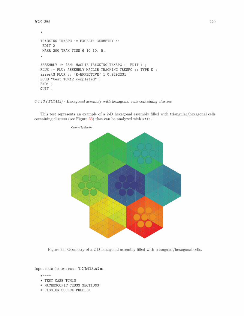
IGE–294 220

;

TRACKING TRKSPC := EXCELT: GEOMETRY ::

EDIT 2

MAXR 200 TRAK TISO 6 10 10. 5.

;

ASSEMBLY := ASM: MACLIB TRACKING TRKSPC :: EDIT 1 ;

FLUX := FLU: ASSEMBLY MACLIB TRACKING TRKSPC :: TYPE K ;



END: ;

QUIT .

6.4.13 (TCM13) - Hexagonal assembly with hexagonal cells containing clusters

This test represents an example of a 2-D hexagonal assembly filled with triangular/hexagonal cellscontaining clusters (see Figure 33) that can be analyzed with NXT:.

Colored by Region

Figure 33: Geometry of a 2-D hexagonal assembly filled with triangular/hexagonal cells.


*----

* TEST CASE TCM13



IGE–294 221

* HEXAGONAL CELL with PINS

*----


*----

LINKED_LIST MacLib GlobalGeo Tracking Pij Flux ;

SEQ_ASCII Fig.ps ;

SEQ_BINARY Lines ;

MODULE MAC: GEO: NXT: PSP: ASM: FLU: DELETE: END: ;

PROCEDURE assertS ;

*----

* Macroscopic XS

*----

MacLib := MAC: ::


READ INPUT

MIX 1 TOTAL 0.166667 1.111111

SCAT 2 2 0.00015 0.126667 2 2 1.10111 0.039

MIX 2 TOTAL 0.166667 1.111111

SCAT 2 2 0.00015 0.126667 2 2 1.10111 0.039

MIX 3 TOTAL 0.166667 1.111111

SCAT 2 2 0.00015 0.126667 2 2 1.10111 0.039

MIX 4 TOTAL 0.166667 1.111111

SCAT 2 2 0.00015 0.126667 2 2 1.10111 0.039

MIX 5 TOTAL 0.166667 1.111111

SCAT 2 2 0.00015 0.126667 2 2 1.10111 0.039

MIX 6 TOTAL 0.166667 1.111111

SCAT 2 2 0.00015 0.126667 2 2 1.10111 0.039

MIX 7 TOTAL 0.166667 1.111111

SCAT 2 2 0.00015 0.126667 2 2 1.10111 0.039

MIX 8 TOTAL 0.166667 1.111111

SCAT 2 2 0.00015 0.126667 2 2 1.10111 0.039

MIX 9 TOTAL 0.166667 1.111111

SCAT 2 2 0.00015 0.126667 2 2 1.10111 0.039

MIX 10 TOTAL 0.166667 1.111111

SCAT 2 2 0.00015 0.126667 2 2 1.10111 0.039

MIX 11 TOTAL 0.166667 1.111111

SCAT 2 2 0.00015 0.126667 2 2 1.10111 0.039

MIX 12 TOTAL 0.166667 1.111111

SCAT 2 2 0.00015 0.126667 2 2 1.10111 0.039

MIX 13 TOTAL 0.166667 1.111111

SCAT 2 2 0.00015 0.126667 2 2 1.10111 0.039

MIX 14 TOTAL 0.166667 1.111111

SCAT 2 2 0.00015 0.126667 2 2 1.10111 0.039

MIX 15 TOTAL 0.166667 1.111111

SCAT 2 2 0.00015 0.126667 2 2 1.10111 0.039

MIX 16 TOTAL 0.166667 1.111111

SCAT 2 2 0.00015 0.126667 2 2 1.10111 0.039

MIX 17 TOTAL 0.222222 0.833333

SCAT 1 1 0.19222 2 2 0.75333 0.02

NUSIGF 0.0 0.170 CHI 1.0 0.0

MIX 18 TOTAL 0.222222 0.833333

SCAT 1 1 0.19222 2 2 0.75333 0.02

NUSIGF 0.0 0.170 CHI 1.0 0.0

;

*----

IGE–294 222

* Geometry : Hexagonal assembly containing

* hexagons with 4 triangular crown and pins

*----

GlobalGeo := GEO: :: HEX 7

HBC COMPLETE REFL

CELL C1 C2 C1 C2 C1 C2 C1

::: C1 := GEO: HEXT 4

SIDE 4.0

MIX

1 2 3 4 5 6 7 8 9 10 11 12 13 14 15 16

1 2 3 4 5 6 7 8 9 10 11 12 13 14 15 16

1 2 3 4 5 6 7 8 9 10 11 12 13 14 15 16

1 2 3 4 5 6 7 8 9 10 11 12 13 14 15 16

1 2 3 4 5 6 7 8 9 10 11 12 13 14 15 16

1 2 3 4 5 6 7 8 9 10 11 12 13 14 15 16

CLUSTER ROD1 ROD2

::: ROD1 := GEO: TUBE 2 MIX 17 18 NPIN 1 RPIN 0.0000 APIN 0.0000

RADIUS 0.00000 0.6122 0.6540 ;

::: ROD2 := GEO: ROD1 MIX 17 18 NPIN 6 RPIN 1.4885 APIN 0.0000 ;

;

::: C2 := GEO: HEXT 4

SIDE 4.0 1.1

MIX

1 2 3 4 5 6 7 8 9 10 11 12 13 14 15 16

1 2 3 4 5 6 7 8 9 10 11 12 13 14 15 16

1 2 3 4 5 6 7 8 9 10 11 12 13 14 15 16

1 2 3 4 5 6 7 8 9 10 11 12 13 14 15 16

1 2 3 4 5 6 7 8 9 10 11 12 13 14 15 16

1 2 3 4 5 6 7 8 9 10 11 12 13 14 15 16

;

;

*----

* Tracking : NXT

* Solution : PIJ

*----

Lines Tracking := NXT: GlobalGeo ::

EDIT 2 LONG NORE TISO 3 10.0 ;

Fig.ps := PSP: Tracking ;

Pij := ASM: MacLib Tracking Lines ;

Flux := FLU: Pij MacLib Tracking :: TYPE K ;

assertS Flux :: ’K-EFFECTIVE’ 1 0.9896834 ;

Flux Pij := DELETE: Flux Pij ;

GlobalGeo Tracking Lines := DELETE: GlobalGeo Tracking Lines ;


END: ;

QUIT "LIST" .

IGE–294 223

6.5 WIMSD4 microscopic cross-section examples.

The test cases we will consider here use the LIB: module to enter microscopic cross sections takenfrom a WIMSD4 69 groups library. We will assume that this library is located in file iaea. The testcases are numbered successively from (TCWU01) to (TCWU31).

6.5.1 (TCWU01) – The Mosteller benchmark.

1

1

3

1.26209 cm

2

Figure 34: Geometry for the Mosteller benchmark problem.

This benchmark uses both a cartesian 2-D cell with a central annular pin and an equivalent annularcell.[83] No depletion information is required in this case since the module EVO: will not be executed. Acomparison between various calculation options is provided here. We first consider the annular geometrywith a SYBILT: self-shielding and a SYBILT: transport calculation. This is then repeated for the cartesian2–D cell. Finally, we used an isotropic (TISO) and a specular (TSPC) EXCELT: tracking successively forthe self-shielding and transport calculations.

Input data for test case: TCWU01.x2m

*----

* TEST CASE TCWU01

* MOSTELLER BENCHMARK: 1-D ANNULAR CELL AND 2-D CARTESIAN CELL

* WIMSD4 69 GROUPS LIBRARY FILE iaea FROM WLUP

*


*

*----


*----

LINKED_LIST

MOSTELA MOSTELC DISCR LIBRARY CP CALC OUT ;

SEQ_BINARY

TRKSPC ;

MODULE

LIB: GEO: SYBILT: EXCELT: SHI: ASM: FLU: EDI: DELETE: END: ;

PROCEDURE assertS ;

*----

* Microscopic cross sections from file iaea format WIMSD4

*----

IGE–294 224

LIBRARY := LIB: ::

NMIX 3 CTRA WIMS

MIXS LIB: WIMSD4 FIL: iaea

MIX 1 600.0 O16 = ’6016’ 4.61309E-2

U235 = ’2235’ 1.66078E-4 1

U238 = ’8238’ 2.28994E-2 1

MIX 2 600.0

Zr91 = ’91’ 3.83243E-2

MIX 3 600.0

H1H2O = ’3001’ 4.42326E-2 O16H2O = ’6016’ 2.21163E-2

BNat = ’1011’ 1.02133E-5

;

*----

* Geometry MOSTELA : annular 3 region geometry

* MOSTELC : Cartesian 3 region geometry

*----


R+ REFL RADIUS 0.0 0.39306 0.45802 0.71206 SPLITR 2 1 1

MIX 1 2 3 ;


X- REFL X+ REFL MESHX 0.0 1.26209

Y- REFL Y+ REFL MESHY 0.0 1.26209

RADIUS 0.0 0.39306 0.45802 SPLITR 2 1

MIX 1 2 3 ;

*----

* Case 1 -- annular




*----

DISCR := SYBILT: MOSTELA ::

TITLE ’TCWU01: MOSTELLER BENCHMARK (SYBIL / SYBIL)’

MAXR 4 QUA1 5 ;

LIBRARY := SHI: LIBRARY DISCR :: EDIT 0 NOLJ ;

CP := ASM: LIBRARY DISCR ;


TYPE K ;


OUT := EDI: LIBRARY DISCR CALC ::

EDIT 4 MERG MIX 1 2 3 COND 4.0 SAVE ;


*----





*----

DISCR := SYBILT: MOSTELC ::

TITLE ’TCWU01: MOSTELLER BENCHMARK (SYBIL / SYBIL)’

MAXR 4 QUA1 5 QUA2 6 5 ;




TYPE K ;


IGE–294 225


EDIT 1 MERG MIX 1 2 3 COND 4.0 STAT ALL REFE 1 ;


*----

* Case 3 -- annular

* Self-Shielding calculation EXCEL-ISO

* Transport calculation EXCEL-ISO


*----


TITLE ’TCWU01: MOSTELLER BENCHMARK (EXCELL)’


LIBRARY := SHI: LIBRARY DISCR TRKSPC :: EDIT 0 NOLJ ;

CP := ASM: LIBRARY DISCR TRKSPC ;


TYPE K ;





*----


* Self-Shielding calculation EXCEL-SPC

* Transport calculation EXCEL-SPC


*----


TITLE ’TCWU01: MOSTELLER BENCHMARK (EXCELL)’

MAXR 4 TRAK TSPC 12 20.0 ;

LIBRARY := SHI: LIBRARY DISCR TRKSPC :: EDIT 0 NOLJ ;

CP := ASM: LIBRARY DISCR TRKSPC ;


TYPE K ;





ECHO "test TCWU01 completed" ;

END: ;

QUIT "LIST" .

6.5.2 (TCWU02) – A 17× 17 PWR type assembly

This test case represents a production calculation of a normal PWR assembly with cell grouping(MERGE and TURN options). Its configuration is shown in Figure 35.


*----

* TEST CASE TCWU02

* 17 X 17 PWR ASSEMBLY WITHOUT POISON


*

* REF: none

IGE–294 226

CL

CL

CL

1 32 2 1 2 2 1 2(1) (3) (12) (11) (12) (12) (11) (12) (15)

(5) (5)(13) (6) (8)

(2) (5) (5) (10) (5) (8)

(13) (5) (6) (6) (5) (6) (8)

(4) (6) (5) (6) (6) (5) (6) (8)

(2) (3) (7) (8)

(13) (7) (8)

(14) (8)

(9)

2 2 2 2 2 2 2 3

2 2 2 2 2 2 3

31 2 2 1 2

2 2 2 2 3

1 2 2 3

2 2 3

2 3

4

(b)

a

1.26472 cm

1.2

64

72

cm

1.2

64

72

cm

1.26472 cm

1.2

64

72

cm

1.31472 cm

1.3

14

72

cm

1.31472 cm

1:empty cell

2:fuel cell

3:boundary cell

4:corner cell

generating cell number

merged cell numberorientation

Figure 35: Geometry for test case (TCWU02).

*

*----


*----

LINKED_LIST

ASSMB DISCR LIBRARY CP CALC OUT DATABASE ISOT SPHGEOM MTRACK ;

SEQ_ASCII

res ;

MODULE

LIB: GEO: SYBILT: BIVACT: SHI: ASM: FLU: EDI: COMPO: SPH: DELETE:

END: ;

PROCEDURE assertS ;

*----


*----

LIBRARY := LIB: ::

NMIX 8 CTRA WIMS

IGE–294 227


MIX 1 579.9

H1H2O = ’3001’ 4.76690E-2 O16H2O = ’6016’ 2.38345E-2

BNat = ’1011’ 2.38103E-5

MIX 2 579.9 O16 = ’6016’ 3.06711E-4

Cr52 = ’52’ 7.54987E-5 Fe56 = ’2056’ 1.47624E-4

Zr91 = ’91’ 4.18621E-2

MIX 3 579.9

H1H2O = ’3001’ 4.65292E-2 O16H2O = ’6016’ 2.32646E-2

Cr52 = ’52’ 4.79927E-5

Fe56 = ’2056’ 4.45845E-5 Ni58 = ’58’ 1.13521E-4

MoNat = ’96’ 4.03755E-6

Al27 = ’27’ 2.35231E-6

Mn55 = ’55’ 4.15901E-7

BNat = ’1011’ 2.32761E-5

Zr91 = ’91’ 8.92427E-4

MIX 4 579.9 O16 = ’6016’ 2.87335E-4

Cr52 = ’52’ 7.07291E-5 Fe56 = ’2056’ 1.38298E-4

Zr91 = ’91’ 3.92175E-2

MIX 5 579.9

H1H2O = ’3001’ 4.71346E-2 O16H2O = ’6016’ 2.35673E-2

Cr52 = ’52’ 2.24991E-5

Fe56 = ’2056’ 2.09013E-5 Ni58 = ’58’ 5.32188E-5

MoNat = ’96’ 1.89281E-6

Al27 = ’27’ 1.10277E-6

Mn55 = ’55’ 1.94976E-7

BNat = ’1011’ 2.35598E-5

Zr91 = ’91’ 4.18372E-4

MIX 6 579.9

H1H2O = ’3001’ 4.71676E-2 O16H2O = ’6016’ 2.35838E-2

Cr52 = ’52’ 2.11122E-5

Fe56 = ’2056’ 1.96130E-5 Ni58 = ’58’ 4.99383E-5

MoNat = ’96’ 1.77614E-6

Al27 = ’27’ 1.03479E-6

Mn55 = ’55’ 1.82957E-7

BNat = ’1011’ 2.35753E-5

Zr91 = ’91’ 3.92583E-4

MIX 7 579.9

H1H2O = ’3001’ 4.72020E-2 O16H2O = ’6016’ 2.36010E-2

Cr52 = ’52’ 1.96591E-5

Fe56 = ’2056’ 1.82630E-5 Ni58 = ’58’ 4.65011E-5

MoNat = ’96’ 1.65389E-6

Al27 = ’27’ 9.63569E-7

Mn55 = ’55’ 1.70365E-7

BNat = ’1011’ 2.35914E-5

Zr91 = ’91’ 3.65562E-4

MIX 8 933.6 O16 = ’6016’ 4.49355E-2

U235 = ’2235’ 7.39237E-4 1

U238 = ’8238’ 2.17285E-2 1

;

*----

* Geometry ASSMB : a 17 X 17 normal PWR assembly

* contains C1 : cell without fuel

* C2 : normal fuel cell

* C3 : peripheral cell

IGE–294 228

* C4 : corner cell

*----

ASSMB := GEO: :: CAR2D 9 9


CELL C1 C2 C2 C1 C2 C2 C1 C2 C3

C2 C2 C2 C2 C2 C2 C2 C3

C2 C2 C2 C2 C2 C2 C3

C1 C2 C2 C1 C2 C3

C2 C2 C2 C2 C3

C1 C2 C2 C3

C2 C2 C3

C2 C3

C4

MERGE 1 3 12 11 12 12 11 12 15

4 6 5 6 6 5 6 8

13 5 6 6 5 6 8

2 5 5 10 5 8

13 5 5 6 8

2 5 7 8

13 7 8

14 8

9

TURN H H B H H B H H A

H G G H G G H A

A E E F E E A

H H F H H A

H E G H A

H H A A

H A A

A A

A

::: C1 := GEO: CARCEL 2

MESHX 0.0 1.26472 MESHY 0.0 1.26472

RADIUS 0.0 0.572435 0.613142 MIX 1 2 3 ;

::: C2 := GEO: C1 RADIUS 0.0 0.412660 0.474364 MIX 8 4 5 ;

::: C3 := GEO: C2 MESHX 0.0 1.31472 MIX 8 4 6 ;

::: C4 := GEO: C3 MESHY 0.0 1.31472 MIX 8 4 7 ;

;

*----



* Flux calculation for B1 homogeneous leakage

* Editing using SPH model for transport-diffusion

*----

DISCR := SYBILT: ASSMB ::

TITLE ’TCWU02: 17 X 17 MULTICELL PWR BENCHMARK WITHOUT POISON’

MAXR 400 QUA2 6 3 ;




TYPE B B1 ;

assertS CALC :: ’K-INFINITY’ 1 1.257190 ;

OUT := EDI: LIBRARY DISCR CALC ASSMB ::

EDIT 3 UPS SAVE MICR RES MERGE CELL COND 4.0

IGE–294 229

;

SPHGEOM := OUT :: STEP UP ’MACRO-GEOM’ ;

MTRACK := BIVACT: SPHGEOM :: PRIM 1 2 EDIT 0 ;

OUT := SPH: OUT MTRACK ;

SPHGEOM MTRACK := DELETE: SPHGEOM MTRACK ;

DATABASE := COMPO: ::

EDIT 5

COMM ’Multi-parameter reactor database’ ENDC

INIT

;

DATABASE := COMPO: DATABASE OUT ::

EDIT 3

;

res := DATABASE ;

ISOT := DATABASE :: STEP UP default

STEP UP MIXTURES STEP AT 5

STEP UP CALCULATIONS STEP AT 1

STEP UP *MAC*RES ;

assertS ISOT :: ’NWT0’ 1 5.186729E-01 ;



END: ;

QUIT "LIST" .

6.5.3 (TCWU03) – An hexagonal assembly

This test case represents a production calculation of a typical hexagonal control assembly. Its config-uration is presented in Figure 36.


*----

* TEST CASE TCWU03

* MULTICELL HEXAGONAL ASSEMBLY WITH POISON

* iaea WLUP Library

*

* REF: none

*

*----


*----

LINKED_LIST

ASSMBH DISCR LIBRARY CP CALC OUT DATABASE ISOT SPHGEOM MTRACK ;

SEQ_ASCII

res ;

MODULE

GEO: SYBILT: BIVACT: LIB: SHI: ASM: FLU: EDI: COMPO: SPH: DELETE:

END: ;

PROCEDURE assertS ;

*----


IGE–294 230

Cricket SoftwareÊÊ

orientation

generating cell number

merged cell number

0.707297 cm

1:empty cell

2:poison cell

3:fuel cell

4:boundary cell

1

(1)

3

(2)

3

(4)

3

(3)

3

(4)

3

(5)

3

(7)

2

(6)

3

(8)

3

(8)

2

(9)

3

(7)

3

(4)

3

(7)

3

(7)

3

(10)

3

(12)

3

(12)

2

(11)

3

(7)2

(14)

3

(15)

3

(12)

3

(16)

3

(17)

3

(19)

3

(18)

3

(18)

3

(16)

3

(12)

4

(23)

4

(22)

4

(22)

4

(21)

4

(21)

4

(20)

a(b)

CL

CL

Figure 36: Geometry for test case (TCWU03).

*----

LIBRARY := LIB: ::

NMIX 11 CTRA WIMS


MIX 1 579.9

H1H2O = ’3001’ 4.76690E-2 O16H2O = ’6016’ 2.38345E-2

BNat = ’1011’ 2.38103E-5

MIX 2 579.9 O16 = ’6016’ 3.06711E-4

Cr52 = ’52’ 7.54987E-5 Fe56 = ’2056’ 1.47624E-4

Zr91 = ’91’ 4.18621E-2

MIX 3 579.9

H1H2O = ’3001’ 4.65292E-2 O16H2O = ’6016’ 2.32646E-2

Cr52 = ’52’ 4.79927E-5

Fe56 = ’2056’ 4.45845E-5 Ni58 = ’58’ 1.13521E-4

MoNat = ’96’ 4.03755E-6

Al27 = ’27’ 2.35231E-6

Mn55 = ’55’ 4.15901E-7

BNat = ’1011’ 2.32761E-5

Zr91 = ’91’ 8.92427E-4

MIX 4 933.6 O16 = ’6016’ 4.49355E-2

U235 = ’2235’ 7.39237E-4 1

U238 = ’8238’ 2.17285E-2 1

MIX 5 579.9 In115 = ’2115’ 7.57464E-3

Cd113 = ’2113’ 2.62493E-3

Ag109 = ’3109’ 4.49188E-2

IGE–294 231

MIX 6 579.9 Cr52 = ’52’ 1.52702E-2

Fe56 = ’2056’ 5.57670E-2 Ni58 = ’58’ 7.51418E-3

Mn55 = ’55’ 8.02943E-4

MIX 7 579.9

H1H2O = ’3001’ 3.06466E-2 O16H2O = ’6016’ 1.53233E-2

Fe56 = ’2056’ 5.27485E-5 Cr52 = ’52’ 2.69769E-5

BNat = ’1011’ 1.53077E-5

Zr91 = ’91’ 1.49580E-2

MIX 8 579.9

H1H2O = ’3001’ 4.65292E-2 O16H2O = ’6016’ 2.32646E-2

Cr52 = ’52’ 4.79927E-5

Fe56 = ’2056’ 4.45845E-5 Ni58 = ’58’ 1.13521E-4

MoNat = ’96’ 4.03755E-6

Al27 = ’27’ 2.35231E-6

Mn55 = ’55’ 4.15901E-7

BNat = ’1011’ 2.32761E-5

Zr91 = ’91’ 8.92427E-4

MIX 9 579.9 O16 = ’6016’ 2.87335E-4

Cr52 = ’52’ 7.07291E-5 Fe56 = ’2056’ 1.38298E-4

Zr91 = ’91’ 3.92175E-2

MIX 10 579.9

H1H2O = ’3001’ 4.71346E-2 O16H2O = ’6016’ 2.35673E-2

Cr52 = ’52’ 2.24991E-5

Fe56 = ’2056’ 2.09013E-5 Ni58 = ’58’ 5.32188E-5

MoNat = ’96’ 1.89281E-6

Al27 = ’27’ 1.10277E-6

Mn55 = ’55’ 1.94976E-7 BNat = ’1011’ 2.35598E-5

Zr91 = ’91’ 4.18372E-4

MIX 11 579.9

H1H2O = ’3001’ 4.71676E-2 O16H2O = ’6016’ 2.35838E-2

Cr52 = ’52’ 2.11122E-5

Fe56 = ’2056’ 1.96130E-5 Ni58 = ’58’ 4.99383E-5

MoNat = ’96’ 1.77614E-6

Al27 = ’27’ 1.03479E-6

Mn55 = ’55’ 1.82957E-7

BNat = ’1011’ 2.35753E-5

Zr91 = ’91’ 3.92583E-4

;

*----

* Geometry ASSMBH : hexagonal assembly with poison


* C2 : poison cell



*----

ASSMBH := GEO: :: HEX 36

HBC S30 REFL

CELL C1 C3 C3 C3 C3 C3 C2 C3 C3 C3 C2 C3 C3 C3 C3 C3 C3 C2

C3 C3 C2 C3 C3 C3 C3 C3 C3 C3 C3 C3 C4 C4 C4 C4 C4 C4

TURN A A A A A A A A B D A I A C F J B A

F A A E E A A E A A A A A A A A A A

MERGE 1 2 3 4 5 4 6 7 8 7 9 8 10 7 7 4 7 11

12 13 14 15 12 16 17 12 16 18 18 19 20 21 21 22 22 23

::: C1 := GEO: HEXCEL 2

SIDE 0.707297 RADIUS 0.0 0.412282 0.475917

IGE–294 232

MIX 1 2 3 ;

::: C2 := GEO: HEXCEL 5

SIDE 0.707297 RADIUS 0.0 0.25057 0.354359 0.436 0.486 0.6125

MIX 5 5 5 6 7 8 ;

::: C3 := GEO: C1 MIX 4 9 10 ;

::: C4 := GEO: C3 MIX 4 9 11 ;

;

*----

* Self-Shielding calculation JPM




*----

DISCR := SYBILT: ASSMBH ::

TITLE ’TCWU03: MULTICELL HEXAGONAL ASSEMBLY WITH POISON’

MAXR 400 MAXZ 15000 QUA2 6 3 ;




TYPE B B1 ;


OUT := EDI: LIBRARY DISCR CALC ASSMBH ::


;

SPHGEOM := OUT :: STEP UP ’MACRO-GEOM’ ;

MTRACK := BIVACT: SPHGEOM :: PRIM 1 2 1 ;

OUT := SPH: OUT MTRACK ;

SPHGEOM MTRACK := DELETE: SPHGEOM MTRACK ;


EDIT 5


INIT

;

DATABASE := COMPO: DATABASE OUT ::

EDIT 3

;

res := DATABASE ;




STEP UP *MAC*RES ;

assertS ISOT :: ’NWT0’ 1 1.442307E+00 ;



END: ;

QUIT "LIST" .

6.5.4 (TCWU04) – A Cylindrical cell with burnup.

This test case represents a burnup calculation for the mosteller annular geometry.

IGE–294 233

U-235

U-236

U-238

Np-237

Pu-238

Pu-239

Pu-240

Pu-241

Pu-242

Am -241

Am -243

Cm -242

Cm -244

Am -242m

(n,γ)

(n,γ)

(n,γ)

(n,γ)

(n,γ)

(n,γ)

(n,γ)(n,γ)

(n,2n)

(n,2n)

(n,γ)

(n,γ)

(n,γ)

(n,γ)

β- β-

β-

β-

β-

β-

β-

β-

β-

β+

α

α

Figure 37: Depletion chain of heavy isotopes.


*----

* TEST CASE TCWU04

* iaea WLUP Library

* ANNULAR MOSTELLER BENCHMARK WITH BURNUP

*


*

*----

IGE–294 234

* Define variables

*----

INTEGER

istep := 1 ;

REAL

evobeg evoend ;

REAL

step2 step3 step4 step5 :=

1.0 27.1739 67.9348 135.8696 ;

*----


*----

PARAMETER res :: ::: SEQ_ASCII res ; ;

LINKED_LIST

LIBRARY MOSTELAS MOSTELA TRACKS TRACK SYS FLUX BURNUP

EDITION DATABASE ISOT ;

MODULE

GEO: SYBILT: LIB: SHI: ASM: FLU: EVO: EDI: COMPO: DELETE: END: ;

PROCEDURE assertS ;

*----

* Depletion data from file iaea format WIMSD4


*----

LIBRARY := LIB: ::

NMIX 3 CTRA WIMS

DEPL LIB: WIMSD4 FIL: iaea


MIX 1 600.0 O16 = ’6016’ 4.61309E-2

U235 = ’2235’ 1.66078E-4 1

U238 = ’8238’ 2.28994E-2 1

U236 = ’236’ 0.0 1

Pu239 = ’6239’ 0.0 1

MIX 2 600.0

Zr91 = ’91’ 3.83243E-2

MIX 3 600.0

H1H2O = ’3001’ 4.42326E-2 O16H2O = ’6016’ 2.21163E-2

BNat = ’1011’ 1.02133E-5

;

*----

* Geometry MOSTELAS : 3 regions annular cell for self-shielding

* MOSTELA : 4 regions annular cell for transport

*----

MOSTELAS := GEO: :: TUBE 3

R+ REFL RADIUS 0.0 0.39306 0.45802 0.71206

MIX 1 2 3 ;

MOSTELA := GEO: MOSTELAS ::

SPLITR 2 1 1 ;

*----

* Create the reactor database

*----


EDIT 5


PARA ’BURN’ IRRA

PARA ’FLUB’ FLUB

IGE–294 235

INIT

;

*----



* Flux calculation for keff with imposed buckling

* using B1 homogeneous leakage model

*----

TRACKS := SYBILT: MOSTELAS ::

TITLE ’TCWU04: MOSTELLER BENCHMARK WITH BURNUP’

EDIT 1 MAXR 3 ;

LIBRARY := SHI: LIBRARY TRACKS :: EDIT 0 NOLJ ;

TRACK := SYBILT: MOSTELA ::

TITLE ’TCWU04: MOSTELLER BENCHMARK WITH BURNUP’

EDIT 1 MAXR 4 ;

SYS := ASM: LIBRARY TRACK ;

FLUX := FLU: SYS LIBRARY TRACK ::


EDITION := EDI: LIBRARY TRACK FLUX ::

EDIT 3 MICR RES MERG COMP COND 4.0 SAVE ;

*----

* Burnup loop: for first step BURNUP is created

* while for other steps it is modified

* two burnup per step:

* 1) get a first approximation of final composition followed

* by a transport calculation

* 2) use approximation for final flux distribution to get a

* better approximation for final composition

*----

EVALUATE evoend := 0.0 ;

WHILE evoend step2 < DO

EVALUATE evobeg := evoend ;

EVALUATE evoend := step2 ;

IF istep 1 = THEN

BURNUP LIBRARY := EVO: LIBRARY FLUX TRACK ::

SAVE <<evobeg>> DAY POWR 36.8

DEPL <<evobeg>> <<evoend>> DAY POWR 36.8

SET <<evoend>> DAY ;

ELSE

BURNUP LIBRARY := EVO: BURNUP LIBRARY FLUX TRACK ::

SAVE <<evobeg>> DAY POWR 36.8

NOEX DEPL <<evobeg>> <<evoend>> DAY POWR 36.8


ENDIF ;


SYS := DELETE: SYS ;


FLUX := FLU: FLUX SYS LIBRARY TRACK ::



SAVE <<evoend>> DAY POWR 36.8

DEPL <<evobeg>> <<evoend>> DAY POWR 36.8



IGE–294 236

SYS := DELETE: SYS ;




EDITION := EDI: EDITION LIBRARY TRACK FLUX ::

EDIT 3 SAVE ;


SAVE <<evoend>> DAY POWR 36.8 ;

DATABASE := COMPO: DATABASE EDITION BURNUP ::

EDIT 3

SET <<evoend>> DAY

;

EVALUATE step2 step3 step4 step5 :=

step3 step4 step5 step2 ;

EVALUATE istep := istep 1 + ;

ENDWHILE ;


res := DATABASE ;




STEP UP *MAC*RES ;




END: ;

QUIT "LIST" .

6.5.5 (TCWU05) – A CANDU-6 type annular cell with burnup.

This test case represents the typical CANDU type cell with an annular moderator region defined inFigure 38. Both its cross section and depletion data are taken from the same WIMSD4 file. Depletioncalculations are performed for 50 day at a fixed power.[26] The microlib is defined by the procedureTCWU05Lib.c2m presented in Section 6.5.19.


*----

* TEST CASE TCWU05

* CANDU-6 ANNULAR CELL

* iaea WLUP Library

* POWER (KW) = 615.00000

* BURN POWER (KW/KG) = 31.97130

* URANIUM MASS = 19.23600

* UO2 REAL DENSITY = 10.59300

* UO2 EFF DENSITY = 10.43750

* UO2 TEMPERATURE = 941.28998

* ENRICHMENT = 0.71140

* COOLANT D2 AT % = 99.222

* MODERATOR D2 AT % = 99.911

IGE–294 237

MODERATOR

CALENDRIA

Figure 38: Geometry of the CANDU-6 cell.

* NUMBER OF DAYS = 50

*

*----

* Define variables and initialize

* Burnup paremeters

* a) Power

* = 31.9713 kw/kg for 0.0 to 300.0 days

* b) Burnup time interval Delt

* = 1 day for 0 to 1 day

* = 4 days for 1 to 5 days





* c) Days with burnup interval changes

* = 1.0, 5.0, 10.0, 50.0, 150.0 and 300.0 days

* d) Burnup control time variables Timei, Timef

* Timei = initial time

* Timef = final time

*----

REAL

Power Delt Timec Timei Timef :=

31.9713 1.0 1.0 0.0 0.0 ;

*----


*----

LINKED_LIST

LIBRARY CANDU6S CANDU6F VOLMATS VOLMATF PIJ FLUX BURNUP EDITION

DATABASE ISOT ;

SEQ_BINARY

INTLINS INTLINF ;

SEQ_ASCII

database ;

MODULE

IGE–294 238

GEO: EXCELT: SHI: ASM: FLU: EVO: EDI: COMPO: DELETE: END: ;

PROCEDURE assertS ;

*----



*----

PROCEDURE TCWU05Lib ;

INTEGER iedit := 1 ;

LIBRARY := TCWU05Lib :: <<iedit>> ;

*----

* Geometry CANDU6S : 13 regions annular cluster for self-shielding

* CANDU6F : 31 regions annular cluster for transport

*----

CANDU6S := GEO: :: TUBE 5

R+ REFL RADIUS 0.00000 5.16890 5.60320 6.44780 6.58750 16.12171

MIX 1 2 3 4 5

CLUSTER ROD1 ROD2 ROD3 ROD4


RADIUS 0.00000 0.6122 0.6540 ;




;

CANDU6F := GEO: CANDU6S :: SPLITR 6 1 1 1 10

::: ROD1 := GEO: ROD1 SPLITR 2 1 ;




;

*----

* Create the reactor database

*----


EDIT 5

STEP UP ’moderator’

COMM ’Multi-parameter reactor database for moderator’ ENDC

INIT

STEP UP ’fuel’

COMM ’Multi-parameter reactor database for fuel’ ENDC

PARA ’BURN’ IRRA

PARA ’FLUB’ FLUB

INIT

;

*----

* Self-Shielding calculation EXCEL

* Transport calculation EXCEL

* Flux calculation for keff

*----

VOLMATS INTLINS := EXCELT: CANDU6S ::

TITLE ’TCWU05: CANDU-6 ANNULAR POWER= 31.971 FUEL TEMP= 941.29’

EDIT 0 MAXR 13 TRAK TISO 5 10.0 SYMM 12 ;

LIBRARY := SHI: LIBRARY VOLMATS INTLINS :: EDIT 0 NOLJ ;

VOLMATF INTLINF := EXCELT: CANDU6F ::



IGE–294 239

PIJ := ASM: LIBRARY VOLMATF INTLINF ;

FLUX := FLU: PIJ LIBRARY VOLMATF ::

TYPE K ;


EDITION := EDI: LIBRARY VOLMATF FLUX ::

COND 4.0 MERGE MIX 0 0 0 0 1 0 0 0 0 0 MICR RES SAVE ON ’moderator’ ;

DATABASE := COMPO: DATABASE EDITION ::

EDIT 3

STEP UP *

;

EDITION := EDI: EDITION LIBRARY VOLMATF FLUX ::

COND 4.0 MERGE COMP MICR 1 Xe135 SAVE ON ’fuel’ ;

*----



*----

WHILE Timei Timec < DO

EVALUATE Timef := Timei Delt + ;

IF Timei 0.0 = THEN

BURNUP LIBRARY := EVO: LIBRARY FLUX VOLMATF ::

DEPL <<Timei>> <<Timef>> DAY POWR <<Power>> ;

ELSE

BURNUP LIBRARY := EVO: BURNUP LIBRARY FLUX VOLMATF ::

NOEX DEPL <<Timei>> <<Timef>> DAY POWR <<Power>> ;

ENDIF ;


PIJ := DELETE: PIJ ;


FLUX := FLU: FLUX PIJ LIBRARY VOLMATF ::

TYPE K ;


SAVE ON ’fuel’ ;


SAVE <<Timef>> DAY POWR <<Power>> ;

DATABASE := COMPO: DATABASE EDITION BURNUP LIBRARY ::

EDIT 3

STEP UP *

SET <<Timef>> DAY

;

*----

* change delta t for burnup and final time if required

*----

IF Timef Timec = THEN

IF Timec 150.0 = THEN

EVALUATE Delt Timec := 50.0 300.0 ;

ENDIF ;



ENDIF ;



ENDIF ;

IF Timec 5.0 = THEN


ENDIF ;

IGE–294 240

IF Timec 1.0 = THEN


ENDIF ;

ENDIF ;

EVALUATE Timei := Timef ;

ENDWHILE ;


*----

* Export and access the database

*----

database := DATABASE ;

ISOT := DATABASE :: STEP UP fuel



STEP UP *MAC*RES ;



ISOT := DELETE: ISOT ;

ISOT := DATABASE :: STEP UP moderator



STEP UP *MAC*RES ;



INTLINF INTLINS := DELETE: INTLINF INTLINS ;


END: ;

QUIT "LIST" .

6.5.6 (TCWU06) – A CANDU-6 type supercell with control rods.

This test case treats both the CANDU cell with a cartesian moderator region (similar to the celldescribed in defined Figure 38) and the supercell containing a stainless steel rod which can be either inthe inserted or extracted position (see Figure 32). Two groups incremental cross sections correspondingto the rod in the inserted and extracted position with respect to the original supercell containing only3–D fuel elements are computed.[26] The microlib is defined by the procedure TCWU05Lib.c2m presentedin Section 6.5.19.


*----

* TEST CASE TCWU06

* CANDU-6 CARTESIAN CELL

* iaea WLUP Library

* STAINLESS STELL RODS IN 3D SUPERCELL

*

* REF: R. Roy et al. Ann. Nucl. Energy 21, 115 (1994)

*

*----


*----

IGE–294 241

LINKED_LIST

LIBRARY LIBRARY2 CANDU6F CANDU6S TRACK SYS FLUX EDITION BCO BCI

SSRODS ;

SEQ_BINARY

INTLIN ;

MODULE

GEO: EXCELT: LIB: SHI: ASM: FLU: EDI: DELETE: END: ;

PROCEDURE assertS ;

*----



*----




*----

* CELL CALCULATION

* Geometry CANDU6S : 14 regions Cartesian cluster for self-shielding

* CANDU6F : 32 regions Cartesian cluster for transport

* BCO : 48 regions 3D Cartesian geometry

* BCI : 48 regions 3D Cartesian geometry

*----

CANDU6S := GEO: :: CARCEL 5

X+ REFL X- REFL MESHX -14.2875 14.2875

Y+ REFL Y- REFL MESHY -14.2875 14.2875

RADIUS 0.00000 5.16890 5.60320 6.44780 6.58750 14.00

MIX 1 2 3 4 5 5



RADIUS 0.00000 0.6122 0.6540 ;




;






;

*----




*----

TRACK INTLIN := EXCELT: CANDU6S ::

TITLE ’TCWU06: CANDU-6 CARTESIAN FUEL TEMP= 941.29’


LIBRARY := SHI: LIBRARY TRACK INTLIN :: EDIT 0 NOLJ ;

TRACK INTLIN := DELETE: TRACK INTLIN ;

TRACK INTLIN := EXCELT: CANDU6F ::



SYS := ASM: LIBRARY TRACK INTLIN ::

EDIT 0 ;

IGE–294 242


TYPE K ;


*----

* Microscopic cross sections from WIMSLIB for stainless steel

* MIX 1,2,3 from EDI: : fuel, structure material and moderator

* MIX 4 stainless steel rods

*----


EDIT 0 MERGE MIX 1 2 2 2 3 1 1 1 1 1 SAVE ON SSRODS ;

SSRODS := EDITION :: STEP UP SSRODS ;

LIBRARY2 := LIB: SSRODS ::

EDIT 0 NMIX 4 CTRA WIMS


MIX 4 345.66 Fe56 = ’2056’ 6.19027E-2

Cr52 = ’52’ 1.56659E-3 Ni58 = ’58’ 6.83337E-3

Si29 = ’29’ 7.79072E-4 C12 = ’2012’ 1.46552E-4

Mn55 = ’55’ 1.25431E-3

;

EDITION TRACK INTLIN SYS FLUX := DELETE:

EDITION TRACK INTLIN SYS FLUX ;

*----

* SUPERCELL CALCULATION

* Geometry BCO : 27 regions 3D Cartesian geometry with rods out

* BCI : 27 regions 3D Cartesian geometry with rods in

*----

BCO := GEO: :: CAR3D 3 2 2

X- REFL X+ SYME Y- REFL Y+ SYME Z- REFL Z+ SYME

CELL M MX MX MX FXY MXY M MX BX MX FXY BXY

TURN A A A F A A A A A F A A

::: M := GEO: CAR3D 1 1 1 MIX 3

MESHX 0.0 7.14375

MESHY 0.0 7.14375

MESHZ -8.25500 8.25500 SPLITZ 2 ;

::: MX := GEO: M MESHX -7.14375 +7.14375 SPLITX 2 ;

::: MXY := GEO: MX MESHY -7.14375 +7.14375 SPLITY 2 ;

::: BX := GEO: CARCELY 2 1 MIX 3 3 3

MESHX -7.14375 7.14375 SPLITX 2

MESHY 0.0 7.14375

MESHZ -8.25500 8.25500 SPLITZ 2

RADIUS 0.0 3.5100 3.8100 ;

::: BXY := GEO: BX MESHY -7.14375 +7.14375 SPLITY 2 ;

::: FXY := GEO: CARCELZ 2 1 MIX 1 2 3

MESHX -7.14375 7.14375 SPLITX 2

MESHY -7.14375 7.14375 SPLITY 2

MESHZ -8.25500 8.25500 SPLITZ 2

RADIUS 0.0 5.16890 6.58750 ;

;

BCI := GEO: BCO ::

::: BX := GEO: BX MIX 3 4 3 ;

::: BXY := GEO: BXY MIX 3 4 3 ;

;

*----



IGE–294 243

* Homogenized properties for rod out

*----

TRACK INTLIN := EXCELT: BCO ::

EDIT 0 MAXR 40 TRAK TISO 2 1.0 ;

SYS := ASM: LIBRARY2 TRACK INTLIN ::

EDIT 0 ;

FLUX := FLU: SYS LIBRARY2 TRACK ::

TYPE K ;


EDITION := EDI: LIBRARY2 TRACK FLUX ::

EDIT 2 MERG COMP COND 4.0 SAVE ON ’NOBC’ ;

SYS TRACK INTLIN := DELETE: SYS TRACK INTLIN ;

*----



* Homogenized properties for rod in

*----

TRACK INTLIN := EXCELT: BCI ::

EDIT 0 MAXR 40 TRAK TISO 2 1.0 ;

SYS := ASM: LIBRARY2 TRACK INTLIN ::

EDIT 0 ;

FLUX := FLU: FLUX SYS LIBRARY2 TRACK ::

TYPE K ;


EDITION := EDI: EDITION LIBRARY2 TRACK FLUX ::

EDIT 2 MERG COMP COND 4.0 STAT DELS REFE ’NOBC’ ;

TRACK INTLIN SYS := DELETE: TRACK INTLIN SYS ;


END: ;

QUIT "LIST" .

6.5.7 (TCWU07) – A CANDU-6 type calculation using various leakage options.

This test case treats the CANDU cell with a cartesian moderator region (similar to the cell de-scribed in defined Figure 38) using various leakage options. The microlib is defined by the procedureTCWU05Lib.c2m presented in Section 6.5.19.


*----

* TEST CASE TCWU07

* CANDU-6 CARTESIAN CELL

* iaea WLUP Library

* TEST VARIOUS LEAKAGE OPTIONS

*

*----


*----

LINKED_LIST

LIBRARY CANDU6S CANDU6T CANDU6SV CANDU6TV TRACK

SYS FLUX EDITION ;

MODULE

GEO: EXCELT: LIB: SHI: ASM: FLU: EDI: DELETE: END: ;

SEQ_BINARY

IGE–294 244

INTLIN ;

PROCEDURE assertS ;

*----



*----




*----

* Geometry CANDU6S : GEOMETRY FOR SELF-SHIELDING (NO VOID)

* CANDU6F : GEOMETRY FOR TRANSPORT (NO VOID)

* CANDU6FV: GEOMETRY FOR TRANSPORT (COOLANT VOID)

* CANDU6FV: GEOMETRY FOR TRANSPORT (COOLANT VOID)

*----




RADIUS 0.00000 5.16890 5.60320 6.44780 6.58750 14.00

MIX 1 2 3 4 5 5



RADIUS 0.00000 0.6122 0.6540 ;




;

CANDU6T := GEO: CANDU6S :: SPLITR 6 1 1 1 10





;

CANDU6SV := GEO: CANDU6S :: MIX 0 2 3 4 5 5 ;

CANDU6TV := GEO: CANDU6SV :: SPLITR 6 1 1 1 10





;

*----

* CASE WITH NO VOID



* Flux TYPE K AND B WITH VARIOUS LEAKAGE OPTIONS

*----

TRACK INTLIN := EXCELT: CANDU6S ::





TRACK INTLIN := EXCELT: CANDU6T ::


EDIT 0 MAXR 32 ANIS 2 TRAK TISO 7 20.0 SYMM 4 ;


IGE–294 245

EDIT 0 PIJK ;


TYPE K ;



EDIT 3 SAVE COND 4.0 TAKE REGI 1 4 7 10 16 24 ;


TYPE B B1 PNL ;





TYPE B B1 HETE ;






EDIT 0 PIJ ECCO ;


TYPE B B1 ECCO ;




FLUX SYS TRACK INTLIN := DELETE: FLUX SYS TRACK INTLIN ;

*----

* CASE WITH COOLANT VOIDED



* Flux TYPE K AND B WITH VARIOUS LEAKAGE OPTIONS

*----

TRACK INTLIN := EXCELT: CANDU6SV ::





TRACK INTLIN := EXCELT: CANDU6TV ::


EDIT 0 MAXR 32 ANIS 2 TRAK TISO 7 20.0 SYMM 4 ;


EDIT 0 PIJK ;


TYPE K ;





TYPE B B1 PNL ;





TYPE B B1 HETE ;



IGE–294 246




EDIT 0 PIJ ECCO ;


TYPE B B1 ECCO ;




FLUX SYS TRACK INTLIN := DELETE: FLUX SYS TRACK INTLIN ;


END: ;

QUIT "LIST" .

6.5.8 (TCWU08) – Burnup of an homogeneous cell.

This case illustrate the burnup of an homogeneous cell that spends the first 1000 days in a reactorbefore being removed. The depletion of the isotopes in this cell for an additional 1000 days outside ofthe core is also investiguated.


*----

* TEST CASE TCWW08

* HOMOGENEOUS DEPLETION CASE

* iaea WLUP Library

*

* REF: None

*

*----

* Define variables

* Burnup paremeters

* a) Power

* = 600.0 kw/kg for 0.0 to 1000.0 days

* = 0.0 kw/kg for 1000.0 to 2000.0 days




* = 100 days for 500 to 1000 days

* = 1000 days for 1000 to 2000 days

* c) Editing time Timec

* = 0.0, 50.0, 500.0, 1000.0 and 2000.0 days

* d) Burnup control time variables Timei, Timef, TotalTime



* TotalTime = Final time reached

* d) Print variable Iprint

* = 1 reduced print

* = 3 full print

*----

REAL

Power Delt Timec Timei Timef TotalTime :=

600.0 10.0 50.0 0.0 0.0 2000.0 ;

INTEGER

IGE–294 247

Iprint := 1 ;

*----


*----

LINKED_LIST

LIBRARY HOM TRACK PIJ FLUX BURNUP EDITION ;

MODULE

GEO: SYBILT: LIB: SHI: ASM: FLU: EVO: EDI: DELETE: END: ;

PROCEDURE assertS ;

*----



*----

LIBRARY := LIB: ::

NMIX 1 CTRA WIMS



MIX 1 300.0 H1 = ’3001’ 2.00000E+1

U235 = ’2235’ 1.0 1

U236 = ’8238’ 0.0 1

;

*----

* Geometry HOM : Homogeneous geometry

*----

HOM := GEO: :: HOMOGE

MIX 1 ;

*----




*----

TRACK := SYBILT: HOM ::

TITLE ’TCWW08: HOMOGENEOUS BENCHMARK WITH BURNUP’ ;

LIBRARY := SHI: LIBRARY TRACK :: EDIT 0 NOLJ ;

PIJ := ASM: LIBRARY TRACK ;

FLUX := FLU: PIJ LIBRARY TRACK ::

TYPE K ;



COND 4.0 MERGE COMP SAVE ;

*----



*----

WHILE Timei TotalTime < DO



EVALUATE Iprint := 3 ;

ELSE

EVALUATE Iprint := 1 ;

ENDIF ;

IF Timei 0.0 = THEN

BURNUP LIBRARY := EVO: LIBRARY FLUX TRACK ::

EDIT <<Iprint>> DEPL <<Timei>> <<Timef>> DAY

POWR <<Power>> ;

IGE–294 248

ELSE


EDIT <<Iprint>> NOEX DEPL <<Timei>> <<Timef>> DAY

POWR <<Power>> ;

ENDIF ;

LIBRARY := SHI: LIBRARY TRACK :: EDIT 0 NOLJ ;


PIJ := ASM: LIBRARY TRACK ;

FLUX := FLU: FLUX PIJ LIBRARY TRACK ::

TYPE K ;

IF Iprint 3 = THEN


SAVE ;

ENDIF ;

*----

* change delta t for burnup, final time and power if required

*----



EVALUATE Power Delt Timec := 0.0 1000.0 2000.0 ;

ENDIF ;



ENDIF ;



ENDIF ;

ENDIF ;


ENDWHILE ;



END: ;

QUIT "LIST" .

6.5.9 (TCWU09) – Testing boundary conditions.

This case test different boundary conditions for the Mosteller cell.


*----

* TEST CASE TCWU09

* MOSTELLER BENCHMARK FOR 1-D ANNULAR CELL

* iaea WLUP Library

* REFLECTIVE AND VOID BC

*

* REF: None

*

*----


*----

LINKED_LIST

MOSTELA MOSTELV VOLMAT LIBRARY PIJ FLUX OUT ;

IGE–294 249

MODULE

LIB: GEO: SYBILT: SHI: ASM: FLU: EDI: DELETE: END: ;

PROCEDURE assertS ;

*----

* Microscopic cross section from file iaea format WIMSD4

*----

LIBRARY := LIB: ::

NMIX 3 CTRA WIMS


MIX 1 600.0 O16 = ’6016’ 4.61309E-2

U235 = ’2235’ 1.66078E-4 1

U238 = ’8238’ 2.28994E-2 1

MIX 2 600.0

Zr91 = ’91’ 3.83243E-2

MIX 3 600.0

H1H2O = ’3001’ 4.42326E-2 O16H2O = ’6016’ 2.21163E-2

BNat = ’1011’ 1.02133E-5

;

*----

* Geometry MOSTELA : Annular cell with reflective BC

* MOSTELV : Annular cell with void BC

*----


RADIUS 0.0 0.39306 0.45802 0.71206

SPLITR 2 1 1

MIX 1 2 3

R+ REFL ;

MOSTELV := GEO: MOSTELA ::

R+ VOID ;

*----




*----

VOLMAT := SYBILT: MOSTELA ::

TITLE ’TCWU09: SYBIL TRACK MOSTELLER BENCHMARK REFLECTIVE BC ’

MAXR 4 QUA1 5 ;

LIBRARY := SHI: LIBRARY VOLMAT :: EDIT 0 NOLJ ;

PIJ := ASM: LIBRARY VOLMAT ;

FLUX := FLU: PIJ LIBRARY VOLMAT ::

TYPE K ;


OUT := EDI: LIBRARY VOLMAT FLUX ::


PIJ VOLMAT := DELETE: PIJ VOLMAT ;

VOLMAT := SYBILT: MOSTELV ::

TITLE ’TCWU09: SYBIL TRACK MOSTELLER BENCHMARK VOID BC ’

MAXR 4 QUA1 5 ;


FLUX := FLU: FLUX PIJ LIBRARY VOLMAT ::

TYPE K ;

assertS FLUX :: ’K-EFFECTIVE’ 1 1.023486E-02 ;

OUT := EDI: OUT LIBRARY VOLMAT FLUX ::


OUT FLUX PIJ LIBRARY VOLMAT := DELETE:

IGE–294 250

OUT FLUX PIJ LIBRARY VOLMAT ;


END: ;

QUIT "LIST" .

6.5.10 (TCWU10) – Fixed source problem in multiplicative media.

This case verify the use of a fixed source inside a cell where fission also takes place.


*----

* TEST CASE TCWU10

* MOSTELLER BENCHMARK FOR 1-D ANNULAR CELL

* iaea WLUP Library

* FIXED SOURCE PROBLEM IN MULTIPLICATIVE MEDIA

*

* REF: None

*

*----


*----

LINKED_LIST

MOSTELA VOLMAT LIBRARY PIJ FLUX OUT ;

MODULE

LIB: MAC: GEO: SYBILT: SHI: ASM: FLU: EDI: DELETE: END: ;

PROCEDURE assertS assertV ;

*----

* Microscopic cross section from file iaea format WIMSD4

* Fixed source of 1.0E5 in group 6

*----

LIBRARY := LIB: ::

EDIT 0 NMIX 3 CTRA WIMS


MIX 1 600.0 O16 = ’6016’ 4.61309E-2

U235 = ’2235’ 1.66078E-4 1

U238 = ’8238’ 2.28994E-2 1

MIX 2 600.0

Zr91 = ’91’ 3.83243E-2

MIX 3 600.0

H1H2O = ’3001’ 4.42326E-2 O16H2O = ’6016’ 2.21163E-2

BNat = ’1011’ 1.02133E-5

;

LIBRARY := MAC: LIBRARY ::

EDIT 0

READ INPUT

MIX 3 FIXE

0.0 0.0 0.0 0.0 0.0 1.0E+5 0.0 0.0 0.0 0.0

0.0 0.0 0.0 0.0 0.0 0.0 0.0 0.0 0.0 0.0

0.0 0.0 0.0 0.0 0.0 0.0 0.0 0.0 0.0 0.0

0.0 0.0 0.0 0.0 0.0 0.0 0.0 0.0 0.0 0.0

0.0 0.0 0.0 0.0 0.0 0.0 0.0 0.0 0.0 0.0

0.0 0.0 0.0 0.0 0.0 0.0 0.0 0.0 0.0 0.0

0.0 0.0 0.0 0.0 0.0 0.0 0.0 0.0 0.0

IGE–294 251

;

*----

* Geometry MOSTELA : Annular cell with reflective BC

*----


RADIUS 0.0 0.39306 0.45802 0.71206

SPLITR 2 1 1

MIX 1 2 3

R+ REFL ;

*----




*----

VOLMAT := SYBILT: MOSTELA ::

TITLE ’TCWU10: SYBIL TRACK MOSTELLER BENCHMARK’

MAXR 4 QUA1 5 ;

LIBRARY := SHI: LIBRARY VOLMAT :: EDIT 0 NOLJ ;


FLUX := FLU: PIJ LIBRARY VOLMAT ::

TYPE K ;


OUT := EDI: LIBRARY VOLMAT FLUX ::

EDIT 4 MERG MIX 1 2 3 COND 4.0 ;


FLUX := FLU: PIJ LIBRARY VOLMAT :: EDIT 99

TYPE S EXTE 30 UNKT 1.0E-3 ;

assertV FLUX :: ’FLUX’ (*GROUP*) 10 (*REGION*) 4 4.291752E+05 ;

OUT := EDI: OUT LIBRARY VOLMAT FLUX ::

EDIT 4 MERG MIX 1 2 3 COND 4.0 ;

OUT FLUX PIJ LIBRARY VOLMAT := DELETE:

OUT FLUX PIJ LIBRARY VOLMAT ;


END: ;

QUIT "LIST" .

6.5.11 (TCWU11) – Two group burnup of a CANDU-6 type cell.

This case is similar to (TCWU05) except that the burnup module uses DRAGON generated two groupstime dependent microscopic cross sections. The microlib is defined by the procedure TCWU05Lib.c2m

presented in Section 6.5.19.


*----

* TEST CASE TCWU11


* iaea WLUP Library

* TWO GROUP BURNUP

* POWER (KW) = 615.00000





IGE–294 252



* COOLANT D2 AT % = 99.222



*

*----

* Define variables

* Burnup paremeters

* a) Power

* = 31.9713 kw/kg for 0.0 to 300.0 days

* b) 69 Groups Burnup time interval Delt

* = 300 day for 0 to 300 day

* c) 2 Groups Burnup time interval Delt








* = 1.0, 5.0, 10.0, 50.0, 150.0 and 300.0 days




*----

REAL


31.9713 1.0 300.0 0.0 0.0 ;

*----


*----

LINKED_LIST LIBRARY ;

LINKED_LIST

CANDU6S CANDU6F VOLMATS VOLMATF PIJ FLUX BURNUP EDITION ;

SEQ_BINARY

INTLINS INTLINF ;

SEQ_ASCII

res ;

MODULE

GEO: EXCELT: LIB: SHI: ASM: FLU: EVO: EDI: SPH: DELETE: END: ;

PROCEDURE assertS ;

*----



*----




*----



*----


R+ REFL RADIUS 0.00000 5.16890 5.60320 6.44780 6.58750 16.12171

IGE–294 253

MIX 1 2 3 4 5



RADIUS 0.00000 0.6122 0.6540 ;




;






;

*----




*----


TITLE ’TCWU11: FEW GROUP BURNUP / SELF-SHIELDING TRACKING’




TITLE ’TCWU11: FEW GROUP BURNUP / TRANSPORT TRACKING’




TYPE K ;


EDITION := EDI: LIBRARY VOLMATF FLUX CANDU6F ::

MERG REGI 6 6 10 7 7 10 1 1 8 8 10 1

1 9 9 10 1 1 2 3 4 5 5 5

5 5 5 5 5 5 5

COND 4.0 MICR ALL SAVE

MGEO CANDU6F

;

EDITION := SPH: EDITION VOLMATF INTLINF ;

*----

* 69 group Burnup

*----


EDIT 3 EXPM 200.0 DEPL <<Timei>> <<Timec>> DAY POWR <<Power>> ;





TYPE K ;


EDITION := EDI: EDITION LIBRARY VOLMATF FLUX CANDU6F ::

MGEO CANDU6F

;


BURNUP FLUX PIJ LIBRARY INTLINS VOLMATS CANDU6S := DELETE:

BURNUP FLUX PIJ LIBRARY INTLINS VOLMATS CANDU6S ;

IGE–294 254

*----

* 2 group Burnup

*----

LIBRARY := EDITION :: STEP UP ’REF-CASE0001’ ;

EDITION := DELETE: EDITION ;



TYPE K ;



EDIT 1 MERGE COMP MICR ALL SAVE ;

EVALUATE Timec := 1.0 ;



IF Timei 0.0 = THEN


EDIT 3 DEPL <<Timei>> <<Timef>> DAY POWR <<Power>> ;

ELSE


EDIT 3 NOEX DEPL <<Timei>> <<Timef>> DAY POWR <<Power>> ;

ENDIF ;




TYPE K ;


SAVE ;

*----


*----


IF Timec 5.0 = THEN


ENDIF ;

IF Timec 1.0 = THEN


ENDIF ;

ENDIF ;


ENDWHILE ;


res := EDITION ;

EDITION BURNUP FLUX PIJ LIBRARY INTLINF VOLMATF CANDU6F := DELETE:

EDITION BURNUP FLUX PIJ LIBRARY INTLINF VOLMATF CANDU6F ;


END: ;

QUIT "LIST" .

6.5.12 (TCWU12) – Mixture composition.

This case illustrates the use of the INFO: module of DRAGON (see Section 3.13) as well as the newCOMB option in the module LIB: (see Section 3.2).

IGE–294 255


*----

* TEST CASE TCWU12

* iaea WLUP Library

* GENERATE A LIBRARY USING INFO AND OTHER OPTIONS

*

* REF: None

*

*----


* Coolant properties

* a) Input

* TempCool = Coolant temperature (K)

* Purity = D2/(D2+H1) Weight % ratio in Coolant

* b) Output

* DensCool = Coolant Density (g/cm**3)

* WH1C = H1 Weight % in Coolant

* WD2C = D2 Weight % in Coolant

* WO16C = O16 Weight % in Coolant

* Fuel properties

* a) Input

* TempFuel = Fuel temperature (K)

* Enrichment = U235/(U235+U238) Weight % ratio in Fuel

* DensFuel = Fuel Density (g/cm**3)

* b) Output

* WU235F = U235 Weight % in Fuel

* WU238F = U238 Weight % in Fuel

* WO16F = O16 Weight % in Fuel

*----

REAL

TempCool Purity TempFuel Enrichment DensFuel :=

560.66 99.95 941.29 0.72 10.437501 ;

REAL

WH1C WD2C WO16C DensCool

WU235F WU238F WO16F ;

*----


*----

LINKED_LIST

LIBRARY ISOT ;

MODULE

LIB: INFO: END: ;

PROCEDURE assertS ;

*----

* Get Coolant properties

*----

ECHO

"Input - Coolant temperature (K) " TempCool ;

ECHO

"Input - D2/(D2+H1) Weight % ratio in Coolant" Purity ;

INFO: ::

TMP: <<TempCool>> K

PUR: <<Purity>> WGT%

CALC DENS WATER >>DensCool<<

LIB: WIMSD4 FIL: iaea

IGE–294 256

ISO: 3 ’3001’ ’3002’ ’6016’

CALC WGT% D2O >>WH1C<< >>WD2C<< >>WO16C<<

;

ECHO

"Output - Coolant Density (g/cm**3)" DensCool ;

ECHO

"Output - H1 Weight % in Coolant " WH1C ;

ECHO

"Output - D2 Weight % in Coolant " WD2C ;

ECHO

"Output - O16 Weight % in Coolant " WO16C ;

*----

* Get Fuel properties

*----

ECHO

"Input - Fuel temperature (K) " TempFuel ;

ECHO

"Input - U235/(U235+U238) Weight % ratio in Fuel" Enrichment ;

ECHO

"Input - Fuel Density (g/cm**3) " DensFuel ;

INFO: ::

ENR: <<Enrichment>> WGT%

LIB: WIMSD4 FIL: iaea

ISO: 3 ’2235’ ’8238’ ’6016’

CALC WGT% UO2 >>WU235F<< >>WU238F<< >>WO16F<<

;

ECHO

"Output - U235 Weight % in Fuel" WU235F ;

ECHO

"Output - U238 Weight % in Fuel" WU238F ;

ECHO

"Output - O16 Weight % in Fuel " WO16F ;

*----


*----

LIBRARY := LIB: ::

NMIX 8 CTRA WIMS


MIX 1 <<TempCool>> <<DensCool>> O16 = ’6016’ <<WO16C>>

D2D2O = ’3002’ <<WD2C>> H1H2O = ’3001’ <<WH1C>>

MIX 2 <<TempFuel>> <<DensFuel>> O16 = ’6016’ <<WO16F>>

U235 = ’2235’ <<WU235F>> 1

U238 = ’8238’ <<WU238F>> 1

MIX 3 COMB 1 0.5 0 0.5

MIX 4 COMB 1 0.1 2 0.9

;

ISOT := LIBRARY :: STEP UP ’U238 0004’ ;

assertS ISOT :: NG 35 5.000504E-01 ;


END: ;

QUIT "LIST" .

IGE–294 257

6.5.13 (TCWU13) – Solution by the method of cyclic characteristics

This case illustrates the use of the MOCC:module of DRAGON for a solution by the transport equationby the method of cyclic characteristics. This test case also uses the embedded DRAGON procedure storedin the TCWU05Lib.c2m file.


*----

* TEST CASE TCWU13

* 17 X 17 PWR ASSEMBLY WITHOUT POISON


*

* REF: none

*

*----


*----

LINKED_LIST

ASSMB DISCR1 DISCR2 LIBRARY CP CALC OUT DATABASE ISOT SPHGEOM

MTRACK ;

SEQ_BINARY FILTRK ;

SEQ_ASCII

res ;

MODULE

LIB: GEO: SYBILT: NXT: BIVACT: SHI: ASM: FLU: EDI: COMPO: SPH:

DELETE: END: ;

PROCEDURE assertS ;

*----


*----

LIBRARY := LIB: ::

NMIX 8 CTRA WIMS


MIX 1 579.9

H1H2O = ’3001’ 4.76690E-2 O16H2O = ’6016’ 2.38345E-2

BNat = ’1011’ 2.38103E-5

MIX 2 579.9 O16 = ’6016’ 3.06711E-4

Cr52 = ’52’ 7.54987E-5 Fe56 = ’2056’ 1.47624E-4

Zr91 = ’91’ 4.18621E-2

MIX 3 579.9

H1H2O = ’3001’ 4.65292E-2 O16H2O = ’6016’ 2.32646E-2

Cr52 = ’52’ 4.79927E-5

Fe56 = ’2056’ 4.45845E-5 Ni58 = ’58’ 1.13521E-4

MoNat = ’96’ 4.03755E-6

Al27 = ’27’ 2.35231E-6

Mn55 = ’55’ 4.15901E-7

BNat = ’1011’ 2.32761E-5

Zr91 = ’91’ 8.92427E-4

MIX 4 579.9 O16 = ’6016’ 2.87335E-4

Cr52 = ’52’ 7.07291E-5 Fe56 = ’2056’ 1.38298E-4

Zr91 = ’91’ 3.92175E-2

MIX 5 579.9

H1H2O = ’3001’ 4.71346E-2 O16H2O = ’6016’ 2.35673E-2

Cr52 = ’52’ 2.24991E-5

IGE–294 258

Fe56 = ’2056’ 2.09013E-5 Ni58 = ’58’ 5.32188E-5

MoNat = ’96’ 1.89281E-6

Al27 = ’27’ 1.10277E-6

Mn55 = ’55’ 1.94976E-7

BNat = ’1011’ 2.35598E-5

Zr91 = ’91’ 4.18372E-4

MIX 6 579.9

H1H2O = ’3001’ 4.71676E-2 O16H2O = ’6016’ 2.35838E-2

Cr52 = ’52’ 2.11122E-5

Fe56 = ’2056’ 1.96130E-5 Ni58 = ’58’ 4.99383E-5

MoNat = ’96’ 1.77614E-6

Al27 = ’27’ 1.03479E-6

Mn55 = ’55’ 1.82957E-7

BNat = ’1011’ 2.35753E-5

Zr91 = ’91’ 3.92583E-4

MIX 7 579.9

H1H2O = ’3001’ 4.72020E-2 O16H2O = ’6016’ 2.36010E-2

Cr52 = ’52’ 1.96591E-5

Fe56 = ’2056’ 1.82630E-5 Ni58 = ’58’ 4.65011E-5

MoNat = ’96’ 1.65389E-6

Al27 = ’27’ 9.63569E-7

Mn55 = ’55’ 1.70365E-7

BNat = ’1011’ 2.35914E-5

Zr91 = ’91’ 3.65562E-4

MIX 8 933.6 O16 = ’6016’ 4.49355E-2

U235 = ’2235’ 7.39237E-4 1

U238 = ’8238’ 2.17285E-2 1

;

*----

* Geometry ASSMB : a 17 X 17 normal PWR assembly




* C4 : corner cell

*----

ASSMB := GEO: :: CAR2D 9 9


CELL C1 C2 C2 C1 C2 C2 C1 C2 C3

C2 C2 C2 C2 C2 C2 C2 C3

C2 C2 C2 C2 C2 C2 C3

C1 C2 C2 C1 C2 C3

C2 C2 C2 C2 C3

C1 C2 C2 C3

C2 C2 C3

C2 C3

C4

::: C1 := GEO: CARCEL 2

MESHX 0.0 1.26472 MESHY 0.0 1.26472

RADIUS 0.0 0.572435 0.613142 MIX 1 2 3 ;

::: C2 := GEO: C1 RADIUS 0.0 0.412660 0.474364 MIX 8 4 5 ;

::: C3 := GEO: C2 MESHX 0.0 1.31472 MIX 8 4 6 ;

::: C4 := GEO: C3 MESHY 0.0 1.31472 MIX 8 4 7 ;

;

*----


IGE–294 259




*----

DISCR1 := SYBILT: ASSMB ::


MAXR 400 QUA2 6 3 ;

DISCR2 FILTRK := NXT: ASSMB ::


TISO 10 20.0 ;

LIBRARY := SHI: LIBRARY DISCR1 :: EDIT 0 NOLJ ;

CP := ASM: LIBRARY DISCR2 FILTRK ;

CALC := FLU: CP LIBRARY DISCR2 ::

TYPE B B1 ;


OUT := EDI: LIBRARY DISCR1 CALC ASSMB ::


;


END: ;

QUIT "LIST" .

6.5.14 (TCWU14) – SPH Homogenisation without tracking

This case illustrates the use of the SPH homogenisation procedure in the EDI: module of DRAGONwhen a tracking data structure is provided as input. This test case also uses the embedded DRAGONprocedure stored in the TCWU05Lib.c2m file.


*----

* TEST CASE TCWU14


* iaea WLUP Library

*----

*----


*----

LINKED_LIST

LIBRARY CANDU6S CANDU6F VOLMATS VOLMATF PIJ FLUX EDITION

DATABASE ISOT ;

SEQ_BINARY

INTLINS INTLINF ;

SEQ_ASCII

database ;

MODULE

GEO: NXT: SHI: ASM: FLU: EDI: DELETE: END: ;

PROCEDURE assertS ;

*----



*----

IGE–294 260




*----



*----


X+ REFL X- REFL

Y+ REFL Y- REFL

MESHX -14.2875 14.2875

MESHY -14.2875 14.2875

RADIUS 0.00000 5.16890 5.60320 6.44780 6.58750 14.00

MIX 1 2 3 4 5 5



RADIUS 0.00000 0.6122 0.6540 ;




;

CANDU6F := GEO: :: CAR2D 2 2

X+ REFL X- REFL

Y+ REFL Y- REFL

CELL F1 F2 F3 F4


MESHX -14.2875 14.2875

MESHY -14.2875 14.2875

RADIUS 0.00000 5.16890 5.60320 6.44780 6.58750 14.00

MIX 1 2 3 4 5 5



RADIUS 0.00000 0.6122 0.6540 ;




;


MESHX -14.2875 14.2875

MESHY -14.2875 14.2875

RADIUS 0.00000 5.16890 5.60320 6.44780 6.58750 14.00

MIX 1 2 3 4 5 5



RADIUS 0.00000 0.6122 0.6540 ;




;


MESHX -14.2875 14.2875

MESHY -14.2875 14.2875

RADIUS 0.00000 5.16890 5.60320 6.44780 6.58750 14.00

MIX 1 2 3 4 5 5


IGE–294 261


RADIUS 0.00000 0.6122 0.6540 ;




;


MESHX -14.2875 14.2875

MESHY -14.2875 14.2875

RADIUS 0.00000 5.16890 5.60320 6.44780 6.58750 14.00

MIX 1 2 3 4 5 5



RADIUS 0.00000 0.6122 0.6540 ;




;

;

*----

* Self-Shielding calculation NXT

* Transport calculation NXT


*----

VOLMATS INTLINS := NXT: CANDU6S ::


EDIT 0 TISO 50 10.0 ;

LIBRARY := SHI: LIBRARY VOLMATS INTLINS ::

EDIT 0 ;

VOLMATF INTLINF := NXT: CANDU6F ::


EDIT 0 TISO 50 10.0 ;



TYPE K ;



COND 4.0 MERGE CELL MICR 1 Xe135 SAVE ON ’fuel’ ;



END: ;

QUIT "LIST" .

6.5.15 (TCWU15) – A CANDU–6 type Cartesian cell with burnup

This test case is similar to TCWU05 except that the cell boundary are Cartesian and the NXT:

tracking module is used. It uses the embedded DRAGON procedure stored in the TCWU05Lib.c2m file.


*----

* TEST CASE TCWU05


* iaea WLUP Library

IGE–294 262

* POWER (KW) = 615.00000







* COOLANT D2 AT % = 99.222



*

*----


* Burnup paremeters

* a) Power

* = 31.9713 kw/kg for 0.0 to 300.0 days









* = 1.0, 5.0, 10.0, 50.0, 150.0 and 300.0 days




*----

REAL


31.9713 1.0 1.0 0.0 0.0 ;

*----


*----

LINKED_LIST

LIBRARY CANDU6S CANDU6F VOLMATS VOLMATF PIJ FLUX BURNUP EDITION

COMPO1 COMPO2 ;

SEQ_BINARY

INTLINS INTLINF ;

SEQ_ASCII

fuel mode ;

MODULE

GEO: NXT: SHI: ASM: FLU: EVO: EDI: CPO:

DELETE: END: ;

*----



*----


PROCEDURE assertS ;



*----


IGE–294 263


*----




RADIUS 0.00000 5.16890 5.60320 6.44780 6.58750 14.00

MIX 1 2 3 4 5 5



RADIUS 0.00000 0.6122 0.6540 ;




;






;

*----




*----

VOLMATS INTLINS := NXT: CANDU6S ::

TITLE ’TCWU05: CANDU-6 CARTESIAN POWER= 31.971 FUEL TEMP= 941.29’

EDIT 0 TRAK TISO 5 10.0 ;


EDIT 0 ;

VOLMATF INTLINF := NXT: CANDU6F ::

TITLE ’TCWU05: CANDU-6 CARTESIAN POWER= 31.971 FUEL TEMP= 941.29’

EDIT 0 TRAK TISO 5 10.0 ;

PIJ := ASM: LIBRARY VOLMATF INTLINF :: ;


TYPE K ;


EDITION := EDI: FLUX LIBRARY VOLMATF ::

COND 4.0 MERGE MIX 0 0 0 0 1 0 0 0 0 0 SAVE ON ’EDITMOD’ ;

EDITION := EDI: EDITION FLUX LIBRARY VOLMATF ::

COND 4.0 MERGE COMP MICR 1 Xe135 SAVE ;

*----



*----



IF Timei 0.0 = THEN


DEPL <<Timei>> <<Timef>> DAY POWR <<Power>> ;

ELSE


NOEX DEPL <<Timei>> <<Timef>> DAY POWR <<Power>> ;

ENDIF ;


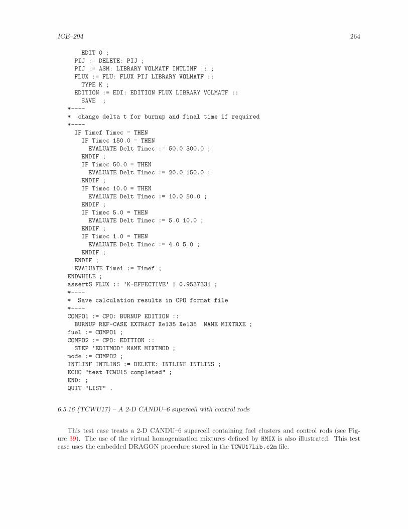
IGE–294 264

EDIT 0 ;


PIJ := ASM: LIBRARY VOLMATF INTLINF :: ;


TYPE K ;

EDITION := EDI: EDITION FLUX LIBRARY VOLMATF ::

SAVE ;

*----


*----




ENDIF ;



ENDIF ;



ENDIF ;

IF Timec 5.0 = THEN


ENDIF ;

IF Timec 1.0 = THEN


ENDIF ;

ENDIF ;


ENDWHILE ;


*----

* Save calculation results in CPO format file

*----

COMPO1 := CPO: BURNUP EDITION ::

BURNUP REF-CASE EXTRACT Xe135 Xe135 NAME MIXTRXE ;

fuel := COMPO1 ;

COMPO2 := CPO: EDITION ::

STEP ’EDITMOD’ NAME MIXTMOD ;

mode := COMPO2 ;



END: ;

QUIT "LIST" .

6.5.16 (TCWU17) – A 2-D CANDU–6 supercell with control rods

This test case treats a 2-D CANDU–6 supercell containing fuel clusters and control rods (see Fig-ure 39). The use of the virtual homogenization mixtures defined by HMIX is also illustrated. This testcase uses the embedded DRAGON procedure stored in the TCWU17Lib.c2m file.

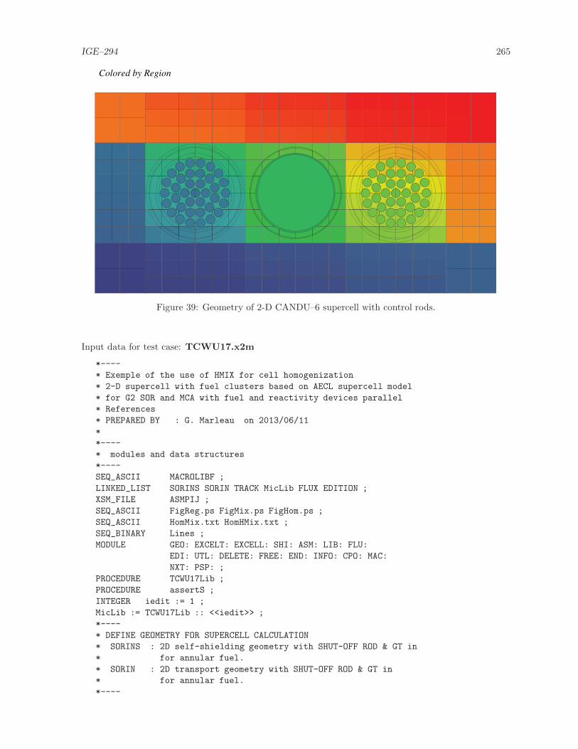
IGE–294 265

Colored by Region

Figure 39: Geometry of 2-D CANDU–6 supercell with control rods.


*----

* Exemple of the use of HMIX for cell homogenization

* 2-D supercell with fuel clusters based on AECL supercell model

* for G2 SOR and MCA with fuel and reactivity devices parallel

* References

* PREPARED BY : G. Marleau on 2013/06/11

*

*----

* modules and data structures

*----

SEQ_ASCII MACROLIBF ;

LINKED_LIST SORINS SORIN TRACK MicLib FLUX EDITION ;

XSM_FILE ASMPIJ ;

SEQ_ASCII FigReg.ps FigMix.ps FigHom.ps ;

SEQ_ASCII HomMix.txt HomHMix.txt ;

SEQ_BINARY Lines ;

MODULE GEO: EXCELT: EXCELL: SHI: ASM: LIB: FLU:

EDI: UTL: DELETE: FREE: END: INFO: CPO: MAC:

NXT: PSP: ;


PROCEDURE assertS ;


MicLib := TCWU17Lib :: <<iedit>> ;

*----

* DEFINE GEOMETRY FOR SUPERCELL CALCULATION

* SORINS : 2D self-shielding geometry with SHUT-OFF ROD & GT in

* for annular fuel.

* SORIN : 2D transport geometry with SHUT-OFF ROD & GT in

* for annular fuel.

*----

IGE–294 266

SORINS := GEO: :: CAR2D 5 3

EDIT 0

X- REFL X+ REFL

Y- REFL Y+ REFL

CELL M MXL MX2 MXR M

MY FXYL BXY FXYR MY

M MXL MX2 MXR M

::: M := GEO: CAR2D 1 1

MESHX 0.0 7.14375

MESHY 0.0 7.14375

HMIX 0

MIX 5 ;

::: MXL := GEO: CAR2D 2 1

MESHX -7.14375 0.0 7.14375

MESHY 0.0 7.14375

HMIX 0 1

MIX 5 15 ;

::: MX2 := GEO: CAR2D 1 1

MESHX -7.14375 7.14375

MESHY 0.0 7.14375

HMIX 1

MIX 15 ;

::: MXR := GEO: CAR2D 2 1

MESHX -7.14375 0.0 7.14375

MESHY 0.0 7.14375

HMIX 1 0

MIX 15 5 ;

::: MY := GEO: CAR2D 1 2

MESHY -7.14375 0.0 7.14375

MESHX 0.0 7.14375

HMIX 0 0

MIX 5 5 ;

::: BXY := GEO: CARCEL 2

MESHX -7.14375 7.14375

MESHY -7.14375 7.14375

RADIUS 0.0 6.380 6.530

HMIX 1 1 1

MIX 15 15 15

CLUSTER ROD

::: ROD := GEO: TUBE 4

NPIN 1 RPIN 0.0 APIN 0.0

RADIUS 0.0 5.4115 5.4877 5.5791 5.6553

HMIX 1 1 1 1

MIX 15 14 21 14 ; ;

::: FXYL := GEO: CARCEL 5 2 1

MESHX -7.14375 0.0 7.14375

MESHY -7.14375 7.14375

RADIUS 0.00000 5.16890 5.60320 6.44780 6.58750 7.00

HMIX 0 0 0 0 0 0

1 1 1 1 1 1

MIX 1 2 3 4 5 5

11 12 13 14 15 15

CLUSTER ROD1 ROD2L ROD2R ROD3L ROD3R ROD4L ROD4R

::: ROD1 := GEO: TUBE 2 1 2 MIX 6 10 16 20 HMIX 0 0 1 1


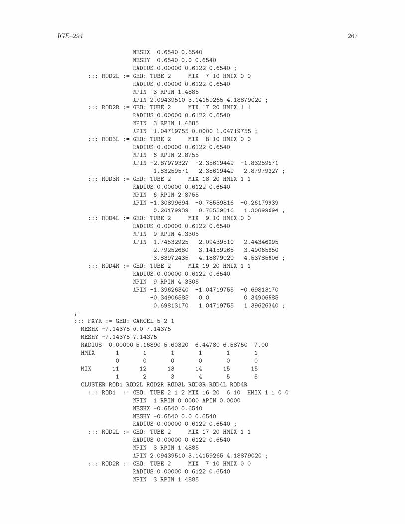
IGE–294 267

MESHX -0.6540 0.6540

MESHY -0.6540 0.0 0.6540

RADIUS 0.00000 0.6122 0.6540 ;

::: ROD2L := GEO: TUBE 2 MIX 7 10 HMIX 0 0

RADIUS 0.00000 0.6122 0.6540

NPIN 3 RPIN 1.4885

APIN 2.09439510 3.14159265 4.18879020 ;

::: ROD2R := GEO: TUBE 2 MIX 17 20 HMIX 1 1

RADIUS 0.00000 0.6122 0.6540

NPIN 3 RPIN 1.4885

APIN -1.04719755 0.0000 1.04719755 ;


RADIUS 0.00000 0.6122 0.6540

NPIN 6 RPIN 2.8755

APIN -2.87979327 -2.35619449 -1.83259571

1.83259571 2.35619449 2.87979327 ;


RADIUS 0.00000 0.6122 0.6540

NPIN 6 RPIN 2.8755

APIN -1.30899694 -0.78539816 -0.26179939

0.26179939 0.78539816 1.30899694 ;


RADIUS 0.00000 0.6122 0.6540

NPIN 9 RPIN 4.3305

APIN 1.74532925 2.09439510 2.44346095

2.79252680 3.14159265 3.49065850

3.83972435 4.18879020 4.53785606 ;


RADIUS 0.00000 0.6122 0.6540

NPIN 9 RPIN 4.3305

APIN -1.39626340 -1.04719755 -0.69813170

-0.34906585 0.0 0.34906585

0.69813170 1.04719755 1.39626340 ;

;

::: FXYR := GEO: CARCEL 5 2 1

MESHX -7.14375 0.0 7.14375

MESHY -7.14375 7.14375

RADIUS 0.00000 5.16890 5.60320 6.44780 6.58750 7.00

HMIX 1 1 1 1 1 1

0 0 0 0 0 0

MIX 11 12 13 14 15 15

1 2 3 4 5 5




MESHX -0.6540 0.6540

MESHY -0.6540 0.0 0.6540

RADIUS 0.00000 0.6122 0.6540 ;


RADIUS 0.00000 0.6122 0.6540

NPIN 3 RPIN 1.4885

APIN 2.09439510 3.14159265 4.18879020 ;


RADIUS 0.00000 0.6122 0.6540

NPIN 3 RPIN 1.4885

IGE–294 268

APIN -1.04719755 0.0000 1.04719755 ;


RADIUS 0.00000 0.6122 0.6540

NPIN 6 RPIN 2.8755

APIN -2.87979327 -2.35619449 -1.83259571

1.83259571 2.35619449 2.87979327 ;


RADIUS 0.00000 0.6122 0.6540

NPIN 6 RPIN 2.8755

APIN -1.30899694 -0.78539816 -0.26179939

0.26179939 0.78539816 1.30899694 ;


RADIUS 0.00000 0.6122 0.6540

NPIN 9 RPIN 4.3305

APIN 1.74532925 2.09439510 2.44346095

2.79252680 3.14159265 3.49065850

3.83972435 4.18879020 4.53785606 ;


RADIUS 0.00000 0.6122 0.6540

NPIN 9 RPIN 4.3305

APIN -1.39626340 -1.04719755 -0.69813170

-0.34906585 0.0 0.34906585

0.69813170 1.04719755 1.39626340 ;

;

;

SORIN := GEO: :: CAR2D 5 3

EDIT 0

X- REFL X+ REFL

Y- REFL Y+ REFL

CELL M MXL MX2 MXR M

MY FXYL BXY FXYR MY

M MXL MX2 MXR M

::: M := GEO: CAR2D 1 1

MESHX 0.0 7.14375 SPLITX 2

MESHY 0.0 7.14375 SPLITY 2

HMIX 0

MIX 5 ;

::: MXL := GEO: CAR2D 2 1

MESHX -7.14375 0.0 7.14375 SPLITX 3 3


HMIX 0 1

MIX 5 15 ;

::: MX2 := GEO: CAR2D 1 1

MESHX -7.14375 7.14375 SPLITX 6


HMIX 1

MIX 15 ;

::: MXR := GEO: CAR2D 2 1

MESHX -7.14375 0.0 7.14375 SPLITX 3 3


HMIX 1 0

MIX 15 5 ;

::: MY := GEO: CAR2D 1 2

MESHY -7.14375 0.0 7.14375 SPLITY 3 3

MESHX 0.0 7.14375 SPLITX 3

IGE–294 269

HMIX 0 0

MIX 5 5 ;

::: BXY := GEO: CARCEL 2

MESHX -7.14375 7.14375 SPLITX 6

MESHY -7.14375 7.14375 SPLITY 6

RADIUS 0.0 6.380 6.530

SPLITR 2 2

HMIX 1 1 1

MIX 15 15 15

CLUSTER ROD

::: ROD := GEO: TUBE 4


RADIUS 0.0 5.4115 5.4877 5.5791 5.6553

SPLITR 1 1 1 1

HMIX 1 1 1 1

MIX 15 14 21 14 ; ;

::: FXYL := GEO: CARCEL 5 2 1

MESHX -7.14375 0.0 7.14375 SPLITX 3 3

MESHY -7.14375 7.14375 SPLITY 6

RADIUS 0.00000 5.16890 5.60320 6.44780 6.58750 7.00

HMIX 0 0 0 0 0 0

1 1 1 1 1 1

MIX 1 2 3 4 5 5

11 12 13 14 15 15




MESHX -0.6540 0.6540

MESHY -0.6540 0.0 0.6540

RADIUS 0.00000 0.6122 0.6540 ;


RADIUS 0.00000 0.6122 0.6540

NPIN 3 RPIN 1.4885

APIN 2.09439510 3.14159265 4.18879020 ;


RADIUS 0.00000 0.6122 0.6540

NPIN 3 RPIN 1.4885

APIN -1.04719755 0.0000 1.04719755 ;


RADIUS 0.00000 0.6122 0.6540

NPIN 6 RPIN 2.8755

APIN -2.87979327 -2.35619449 -1.83259571

1.83259571 2.35619449 2.87979327 ;


RADIUS 0.00000 0.6122 0.6540

NPIN 6 RPIN 2.8755

APIN -1.30899694 -0.78539816 -0.26179939

0.26179939 0.78539816 1.30899694 ;


RADIUS 0.00000 0.6122 0.6540

NPIN 9 RPIN 4.3305

APIN 1.74532925 2.09439510 2.44346095

2.79252680 3.14159265 3.49065850

3.83972435 4.18879020 4.53785606 ;


IGE–294 270

RADIUS 0.00000 0.6122 0.6540

NPIN 9 RPIN 4.3305

APIN -1.39626340 -1.04719755 -0.69813170

-0.34906585 0.0 0.34906585

0.69813170 1.04719755 1.39626340 ;

;

::: FXYR := GEO: CARCEL 5 2 1

MESHX -7.14375 0.0 7.14375 SPLITX 3 3

MESHY -7.14375 7.14375 SPLITY 6

RADIUS 0.00000 5.16890 5.60320 6.44780 6.58750 7.00

HMIX 1 1 1 1 1 1

0 0 0 0 0 0

MIX 11 12 13 14 15 15

1 2 3 4 5 5




MESHX -0.6540 0.6540

MESHY -0.6540 0.0 0.6540

RADIUS 0.00000 0.6122 0.6540 ;


RADIUS 0.00000 0.6122 0.6540

NPIN 3 RPIN 1.4885

APIN 2.09439510 3.14159265 4.18879020 ;


RADIUS 0.00000 0.6122 0.6540

NPIN 3 RPIN 1.4885

APIN -1.04719755 0.0000 1.04719755 ;


RADIUS 0.00000 0.6122 0.6540

NPIN 6 RPIN 2.8755

APIN -2.87979327 -2.35619449 -1.83259571

1.83259571 2.35619449 2.87979327 ;


RADIUS 0.00000 0.6122 0.6540

NPIN 6 RPIN 2.8755

APIN -1.30899694 -0.78539816 -0.26179939

0.26179939 0.78539816 1.30899694 ;


RADIUS 0.00000 0.6122 0.6540

NPIN 9 RPIN 4.3305

APIN 1.74532925 2.09439510 2.44346095

2.79252680 3.14159265 3.49065850

3.83972435 4.18879020 4.53785606 ;


RADIUS 0.00000 0.6122 0.6540

NPIN 9 RPIN 4.3305

APIN -1.39626340 -1.04719755 -0.69813170

-0.34906585 0.0 0.34906585

0.69813170 1.04719755 1.39626340 ;

;

;

*----

* Rod and GT absent

*----

IGE–294 271

TRACK Lines := NXT: SORINS :: EDIT 5 TISO 40 30.0 ;

MicLib := SHI: MicLib TRACK Lines ;

TRACK Lines := DELETE: TRACK Lines ;

TRACK Lines := NXT: SORIN :: EDIT 5 TISO 40 30.0 ;

FigReg.ps := PSP: TRACK :: TYPE REGI ;

FigMix.ps := PSP: TRACK :: TYPE MIXT ;

FigHom.ps := PSP: TRACK :: TYPE HMIX ;

ASMPIJ := ASM: MicLib TRACK Lines :: PIJ ;

FLUX := FLU: ASMPIJ MicLib TRACK :: TYPE K ;


EDITION := EDI: FLUX MicLib TRACK ::

EDIT 3

COND 0.625

MERG HMIX

SAVE ON SORINHMIX ;

HomHMix.txt := EDITION ;


EDITION := EDI: FLUX MicLib TRACK ::

EDIT 3

COND 0.625

MERG MIX 0 0 0 0 0 0 0 0 0 0 1 1 1 1 1 1 1 1 1 1 1

SAVE ON SORINMIX ;

HomMix.txt := EDITION ;


TRACK FLUX ASMPIJ Lines := DELETE: TRACK FLUX ASMPIJ Lines ;


END: ;

QUIT "LIST" .

6.5.17 (TCWU17Lib) – Microlib definition.

This CLE-2000 procedure is used in data-set TCWU17 to define the microlib isotopic content.

Input data for test case: TCWU17Lib.c2m

*----

* Create Library for test CASE TCWU17.x2m

* Calling :

* LIBRARY := TCWU17Lib.x2m :: iedit ;

* with :

* LIBRARY = Linked list containing the result of LIB: for

* TCWU17.x2m

* iprint = print level for LIB: module

*----

* Define PARAMETERS,STRUCTURES and MODULES used

*----

PARAMETER LIBRARY :: ::: LINKED_LIST LIBRARY ; ;

MODULE LIB: DELETE: END: ;

*----

* Define and read LIB: EDIT option

INTEGER iedit ;

:: >>iedit<< ;

*----


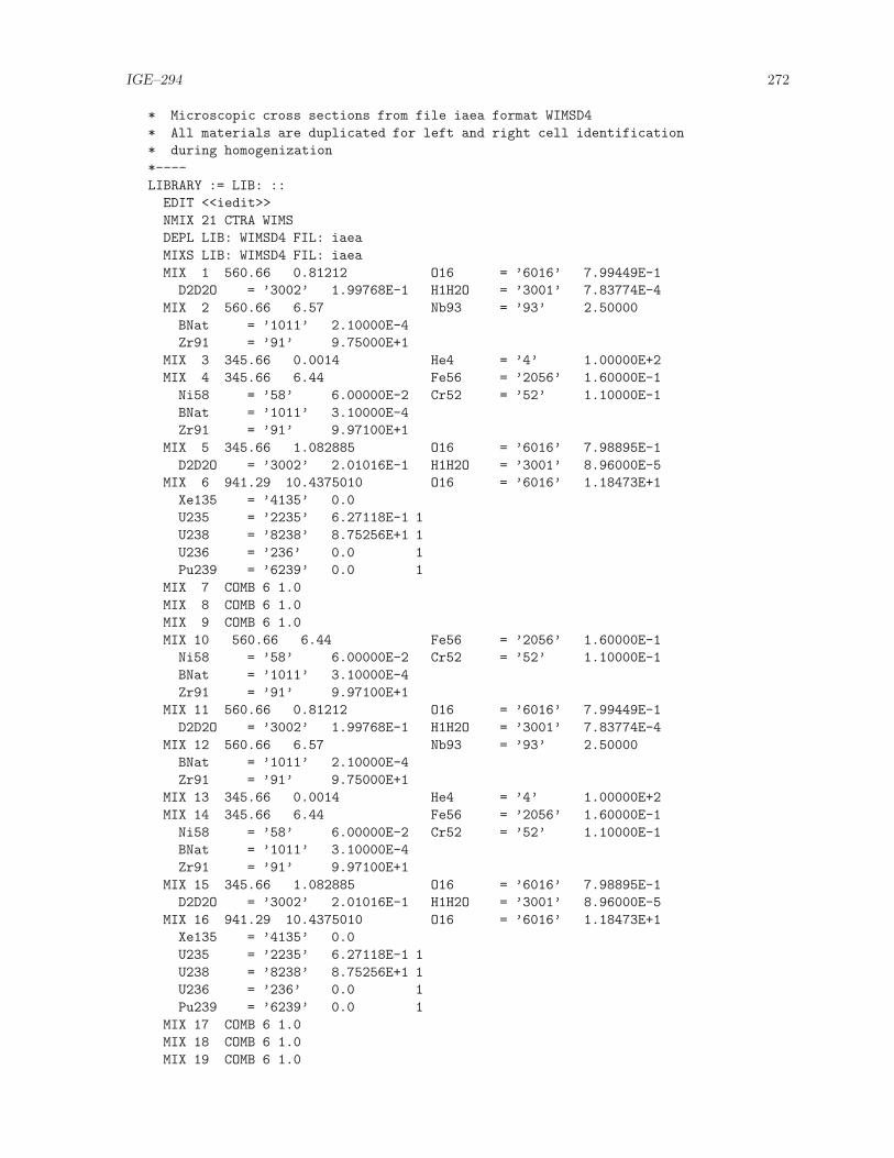
IGE–294 272


* All materials are duplicated for left and right cell identification

* during homogenization

*----

LIBRARY := LIB: ::

EDIT <<iedit>>

NMIX 21 CTRA WIMS



MIX 1 560.66 0.81212 O16 = ’6016’ 7.99449E-1

D2D2O = ’3002’ 1.99768E-1 H1H2O = ’3001’ 7.83774E-4

MIX 2 560.66 6.57 Nb93 = ’93’ 2.50000

BNat = ’1011’ 2.10000E-4

Zr91 = ’91’ 9.75000E+1

MIX 3 345.66 0.0014 He4 = ’4’ 1.00000E+2

MIX 4 345.66 6.44 Fe56 = ’2056’ 1.60000E-1

Ni58 = ’58’ 6.00000E-2 Cr52 = ’52’ 1.10000E-1

BNat = ’1011’ 3.10000E-4

Zr91 = ’91’ 9.97100E+1

MIX 5 345.66 1.082885 O16 = ’6016’ 7.98895E-1

D2D2O = ’3002’ 2.01016E-1 H1H2O = ’3001’ 8.96000E-5

MIX 6 941.29 10.4375010 O16 = ’6016’ 1.18473E+1

Xe135 = ’4135’ 0.0

U235 = ’2235’ 6.27118E-1 1

U238 = ’8238’ 8.75256E+1 1

U236 = ’236’ 0.0 1

Pu239 = ’6239’ 0.0 1

MIX 7 COMB 6 1.0

MIX 8 COMB 6 1.0

MIX 9 COMB 6 1.0

MIX 10 560.66 6.44 Fe56 = ’2056’ 1.60000E-1

Ni58 = ’58’ 6.00000E-2 Cr52 = ’52’ 1.10000E-1

BNat = ’1011’ 3.10000E-4

Zr91 = ’91’ 9.97100E+1

MIX 11 560.66 0.81212 O16 = ’6016’ 7.99449E-1

D2D2O = ’3002’ 1.99768E-1 H1H2O = ’3001’ 7.83774E-4

MIX 12 560.66 6.57 Nb93 = ’93’ 2.50000

BNat = ’1011’ 2.10000E-4

Zr91 = ’91’ 9.75000E+1

MIX 13 345.66 0.0014 He4 = ’4’ 1.00000E+2

MIX 14 345.66 6.44 Fe56 = ’2056’ 1.60000E-1

Ni58 = ’58’ 6.00000E-2 Cr52 = ’52’ 1.10000E-1

BNat = ’1011’ 3.10000E-4

Zr91 = ’91’ 9.97100E+1

MIX 15 345.66 1.082885 O16 = ’6016’ 7.98895E-1

D2D2O = ’3002’ 2.01016E-1 H1H2O = ’3001’ 8.96000E-5

MIX 16 941.29 10.4375010 O16 = ’6016’ 1.18473E+1

Xe135 = ’4135’ 0.0

U235 = ’2235’ 6.27118E-1 1

U238 = ’8238’ 8.75256E+1 1

U236 = ’236’ 0.0 1

Pu239 = ’6239’ 0.0 1

MIX 17 COMB 6 1.0

MIX 18 COMB 6 1.0

MIX 19 COMB 6 1.0

IGE–294 273

MIX 20 560.66 6.44 Fe56 = ’2056’ 1.60000E-1

Ni58 = ’58’ 6.00000E-2 Cr52 = ’52’ 1.10000E-1

BNat = ’1011’ 3.10000E-4

Zr91 = ’91’ 9.97100E+1

MIX 21 345.66 Fe56 = ’2056’ 6.19027E-2

Cr52 = ’52’ 1.56659E-3 Ni58 = ’58’ 6.83337E-3

Si29 = ’29’ 7.79072E-4 C12 = ’2012’ 1.46552E-4

Mn55 = ’55’ 1.25431E-3

;

END: ;

QUIT "LIST" .

6.5.18 (TCWU31) – Compo-based two group burnup of a CANDU-6 type cell.

This case is similar to (TCWU11) except that the two-group burnup calculation recover all its infor-mation from a compo database. The microlib is defined by the procedure TCWU05Lib.c2m presentedin Section 6.5.19.


*----

* TEST CASE TCWU31


* iaea WLUP Library

* MULTI-PARAMETER COMPO ACCESS FOR MACRO-DEPLETION

* TWO GROUP BURNUP

* POWER (KW) = 615.00000







* COOLANT D2 AT % = 99.222



*

*----

* Define variables

* Burnup paremeters

* a) Power

* = 31.9713 kw/kg for 0.0 to 300.0 days

* b) 69 Groups Burnup time interval Delt

* = 300 day for 0 to 300 day

* c) 2 Groups Burnup time interval Delt








* = 1.0, 5.0, 10.0, 50.0, 150.0 and 300.0 days


IGE–294 274



*----

REAL


31.9713 1.0 300.0 0.0 0.0 ;

*----


*----

LINKED_LIST LIBRARY ;

LINKED_LIST

CANDU6S CANDU6F VOLMATS VOLMATF PIJ FLUX BURNUP EDITION DATABASE ;

SEQ_BINARY

INTLINS INTLINF ;

SEQ_ASCII

res ;

MODULE

GEO: EXCELT: LIB: SHI: ASM: FLU: EVO: EDI: COMPO: SPH: DELETE: END: ;

PROCEDURE assertS ;

*----



*----




*----



*----


R+ REFL RADIUS 0.00000 5.16890 5.60320 6.44780 6.58750 16.12171

MIX 1 2 3 4 5



RADIUS 0.00000 0.6122 0.6540 ;




;






;

*----




*----


TITLE ’TCWU31: FEW GROUP BURNUP / SELF-SHIELDING TRACKING’



IGE–294 275






TYPE K ;


EDITION := EDI: LIBRARY VOLMATF FLUX CANDU6F ::

MERG REGI 6 6 10 7 7 10 1 1 8 8 10 1

1 9 9 10 1 1 2 3 4 5 5 5

5 5 5 5 5 5 5

COND 4.0 MICR ALL SAVE

MGEO CANDU6F

;


FLUX PIJ LIBRARY INTLINS VOLMATS CANDU6S VOLMATF CANDU6F

INTLINF := DELETE: FLUX PIJ LIBRARY INTLINS VOLMATS CANDU6S

VOLMATF CANDU6F INTLINF ;

*----

* 2 group Burnup (macro-depletion)

*----


EDIT 5


INIT

;

DATABASE := COMPO: DATABASE EDITION ::

EDIT 3

;


*

* COMPO INTERPOLATION

LIBRARY := SPH: DATABASE ::

EDIT 1

STEP UP default STEP AT 1

MICRO OFF

;

CANDU6F := DATABASE :: STEP UP default STEP UP ’GEOMETRIES’ STEP AT 1 ;






TYPE K ;



EDIT 1 MERGE COMP MICR ALL SAVE ;

EVALUATE Timec := 1.0 ;



IF Timei 0.0 = THEN


EDIT 3 DEPL <<Timei>> <<Timef>> DAY POWR <<Power>> ;

ELSE


IGE–294 276

EDIT 3 NOEX DEPL <<Timei>> <<Timef>> DAY POWR <<Power>> ;

ENDIF ;




TYPE K ;


SAVE ;

*----


*----


IF Timec 5.0 = THEN


ENDIF ;

IF Timec 1.0 = THEN


ENDIF ;

ENDIF ;


ENDWHILE ;


res := EDITION ;

EDITION BURNUP FLUX PIJ LIBRARY INTLINF VOLMATF CANDU6F := DELETE:

EDITION BURNUP FLUX PIJ LIBRARY INTLINF VOLMATF CANDU6F ;


END: ;

QUIT "LIST" .

6.5.19 (TCWU05Lib) – Microlib definition.

This CLE-2000 procedure is used in previous data-sets to define the microlib isotopic content.

Input data for test case: TCWU05Lib.c2m

*----

* Procedure TCWU05Lib

* Create Library for test CASE TCWU05

* Calling :

* LIBRARY := TCWU05Lib :: iedit ;

* with :

* LIBRARY = Linked list containing the result of LIB: for

* TCWU05

* iprint = print level for LIB: module

*----

* Define PARAMETERS,STRUCTURES and MODULES used

*----


MODULE LIB: END: ;

*----

* Define and read LIB: EDIT option

INTEGER iedit ;

:: >>iedit<< ;

*----

IGE–294 277



*----

LIBRARY := LIB: ::

EDIT <<iedit>>

NMIX 17 CTRA WIMS



MIX 1 560.66 0.81212 O16 = ’6016’ 7.99449E-1

D2D2O = ’3002’ 1.99768E-1 H1H2O = ’3001’ 7.83774E-4

MIX 2 560.66 6.57 Nb93 = ’93’ 2.50000

BNat = ’1011’ 2.10000E-4

Zr91 = ’91’ 9.75000E+1

MIX 3 345.66 0.0014 He4 = ’4’ 1.00000E+2

MIX 4 345.66 6.44 Fe56 = ’2056’ 1.60000E-1

Ni58 = ’58’ 6.00000E-2 Cr52 = ’52’ 1.10000E-1

BNat = ’1011’ 3.10000E-4

Zr91 = ’91’ 9.97100E+1

MIX 5 345.66 1.082885 O16 = ’6016’ 7.98895E-1

D2D2O = ’3002’ 2.01016E-1 H1H2O = ’3001’ 8.96000E-5

MIX 6 941.29 10.4375010 O16 = ’6016’ 1.18473E+1

Xe135 = ’4135’ 0.0

U235 = ’2235’ 6.27118E-1 1

U238 = ’8238’ 8.75256E+1 1

U236 = ’236’ 0.0 1

Pu239 = ’6239’ 0.0 1

MIX 7 COMB 6 1.0

MIX 8 COMB 6 1.0

MIX 9 COMB 6 1.0

MIX 10 560.66 6.44 Fe56 = ’2056’ 1.60000E-1

Ni58 = ’58’ 6.00000E-2 Cr52 = ’52’ 1.10000E-1

BNat = ’1011’ 3.10000E-4

Zr91 = ’91’ 9.97100E+1

MIX 11 COMB 10 1.0

MIX 12 COMB 10 1.0

MIX 13 COMB 10 1.0

MIX 14 COMB 1 1.0

MIX 15 COMB 1 1.0

MIX 16 COMB 1 1.0

MIX 17 COMB 1 1.0

;

END: ;

QUIT "LIST" .

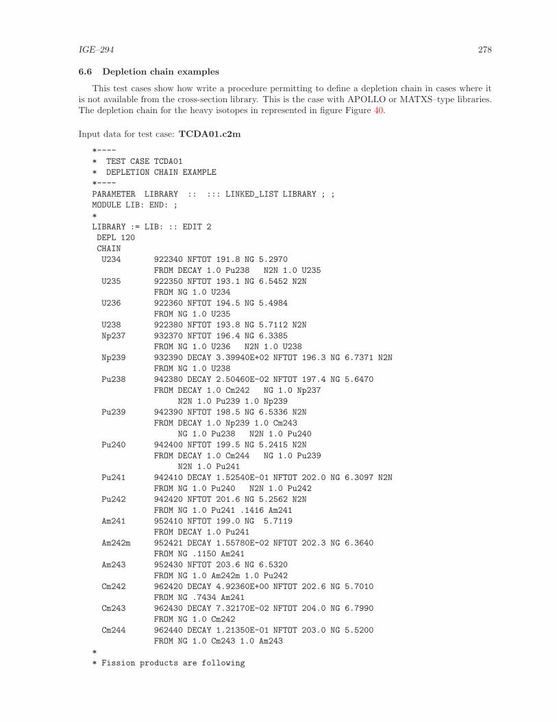
IGE–294 278

6.6 Depletion chain examples

This test cases show how write a procedure permitting to define a depletion chain in cases where itis not available from the cross-section library. This is the case with APOLLO or MATXS–type libraries.The depletion chain for the heavy isotopes in represented in figure Figure 40.

Input data for test case: TCDA01.c2m

*----

* TEST CASE TCDA01

* DEPLETION CHAIN EXAMPLE

*----


MODULE LIB: END: ;

*

LIBRARY := LIB: :: EDIT 2

DEPL 120

CHAIN

U234 922340 NFTOT 191.8 NG 5.2970

FROM DECAY 1.0 Pu238 N2N 1.0 U235

U235 922350 NFTOT 193.1 NG 6.5452 N2N

FROM NG 1.0 U234

U236 922360 NFTOT 194.5 NG 5.4984

FROM NG 1.0 U235

U238 922380 NFTOT 193.8 NG 5.7112 N2N

Np237 932370 NFTOT 196.4 NG 6.3385

FROM NG 1.0 U236 N2N 1.0 U238

Np239 932390 DECAY 3.39940E+02 NFTOT 196.3 NG 6.7371 N2N

FROM NG 1.0 U238

Pu238 942380 DECAY 2.50460E-02 NFTOT 197.4 NG 5.6470

FROM DECAY 1.0 Cm242 NG 1.0 Np237

N2N 1.0 Pu239 1.0 Np239

Pu239 942390 NFTOT 198.5 NG 6.5336 N2N

FROM DECAY 1.0 Np239 1.0 Cm243

NG 1.0 Pu238 N2N 1.0 Pu240

Pu240 942400 NFTOT 199.5 NG 5.2415 N2N

FROM DECAY 1.0 Cm244 NG 1.0 Pu239

N2N 1.0 Pu241

Pu241 942410 DECAY 1.52540E-01 NFTOT 202.0 NG 6.3097 N2N

FROM NG 1.0 Pu240 N2N 1.0 Pu242

Pu242 942420 NFTOT 201.6 NG 5.2562 N2N

FROM NG 1.0 Pu241 .1416 Am241

Am241 952410 NFTOT 199.0 NG 5.7119

FROM DECAY 1.0 Pu241

Am242m 952421 DECAY 1.55780E-02 NFTOT 202.3 NG 6.3640

FROM NG .1150 Am241

Am243 952430 NFTOT 203.6 NG 6.5320

FROM NG 1.0 Am242m 1.0 Pu242

Cm242 962420 DECAY 4.92360E+00 NFTOT 202.6 NG 5.7010

FROM NG .7434 Am241

Cm243 962430 DECAY 7.32170E-02 NFTOT 204.0 NG 6.7990

FROM NG 1.0 Cm242

Cm244 962440 DECAY 1.21350E-01 NFTOT 203.0 NG 5.5200

FROM NG 1.0 Cm243 1.0 Am243

*

* Fission products are following

IGE–294 279

U-234

U-235

U-236

U-238

Np-237

Pu-238

Pu-239

Pu-240

Pu-241

Pu-242

Np-239

Am-241

Am-242m

Am-243

Cm-242

Cm-243

Cm-244

α

α

α

α

β−

β−

β−

β−

β−

β−

β−

β−

β+

(n,2n)(n,2n)

(n,2n)

(n,2n)

(n,γ)

(n,γ)

(n,γ)

(n,γ)

(n,γ)

(n,γ)

(n,γ)

(n,γ)

β−

β−

(n,2n)

(n,2n)

(n,2n)

(n,γ)

(n,γ) (n,γ)

(n,γ) (n,γ)

(n,γ)

(n,γ)

Figure 40: An example of depletion chain.

Zr95 400950 DECAY 1.25390E+01 NG 7.8377

FROM NFTOT 6.463E-02 U235 5.113E-02 U238

4.897E-02 Pu239 4.369E-02 Pu240

IGE–294 280

3.916E-02 Pu241 4.113E-02 Pu242

3.830E-02 Am241 3.311E-02 Am242m

Zr96 400960 NG 5.5751

FROM NFTOT 6.248E-02 U235 5.977E-02 U238

5.002E-02 Pu239 4.941E-02 Pu240

4.376E-02 Pu241 4.575E-02 Pu242

4.551E-02 Am241 3.630E-02 Am242m

NG 1.0 Zr95

(example truncated)

*

* Stable isotopes producing energy are following

Fe54 NG 9.2990 STABLE




Cr50 NG 9.2930 STABLE




Ni58 NG 9.0000 STABLE





Mn55 NG 9.7554 STABLE

H2O NG 2.2251 STABLE

Zr-nat NG 8.1395 STABLE

O16 NG 4.1434 STABLE

Mo95 NG 9.1540 STABLE

Nb93 NG 7.2139 STABLE

Ti-nat NG 8.5137 STABLE

ENDCHAIN ;

*

END: ;

IGE–294 281

6.7 Assert procedures

These two procedures are used in non-regression testcases to ensure that existing capabilities of Dragonare not lost with subsequent updates of the code. Procedure assertS is used to assert a single real valuetaken from record KEY of a LCM associative table. Its calling specification is

Table 101: Structure assertS

assertS LCMNAM :: KEY ipos value ;

where

LCMNAM character*12 name of the LCM data structure.

KEY character*12 name of the real array we want to assert.

ipos integer index of the component in the real array we want to assert.

values real reference value of the ipos–th component.

Procedure assertV is used to assert a single real value taken from an heterogeneous list (named KEY)where each component is a real array. Its calling specification is

Table 102: Structure assertV

assertV LCMNAM :: KEY iset ipos value ;

where

LCMNAM character*12 name of the LCM data structure.

KEY character*12 name of the heterogeneous list we want to assert.

ipos integer index of the component in the heterogeneous list

ipos integer index of the component in the real array we want to assert.

values real reference value of the ipos–th component.

Input data for test case: assertS.c2m

*

* Assert procedure for non-regression testing

* Recover a value from a real array

* Author: A. Hebert

*

PARAMETER LCMNAM :: ::: LINKED_LIST LCMNAM ; ;

CHARACTER KEY ;

INTEGER ISET IPOS ;

REAL REFVALUE ;

:: >>KEY<< >>IPOS<< >>REFVALUE<< ;

INTEGER ITYLCM ;

IGE–294 282

REAL VALUE DELTA ;

MODULE GREP: ABORT: END: ;

*

GREP: LCMNAM :: TYPE <<KEY>> >>ITYLCM<< ;

IF ITYLCM 2 = THEN

GREP: LCMNAM :: GETVAL <<KEY>> <<IPOS>> >>VALUE<< ;

ELSE

PRINT "assertS: INVALID TYPE=" ITYLCM ;

ABORT: ;

ENDIF ;

EVALUATE DELTA := VALUE REFVALUE - REFVALUE / ABS ;

IF DELTA 1.0E-4 < THEN

PRINT "TEST SUCCESSFUL; DELTA=" DELTA ;

ELSE

PRINT "------------" ;

PRINT "TEST FAILURE" ;

PRINT "------------" ;

PRINT "REFERENCE=" REFVALUE " CALCULATED=" VALUE ;

ABORT: ;

ENDIF ;

END: ;

Input data for test case: assertV.c2m

*

* Assert procedure for non-regression testing

* Recover a value from a list of real arrays

* Author: A. Hebert

*

PARAMETER LCMNAM :: ::: LINKED_LIST LCMNAM ; ;

CHARACTER KEY ;

INTEGER ISET IPOS ;

REAL REFVALUE ;

:: >>KEY<< >>ISET<< >>IPOS<< >>REFVALUE<< ;

INTEGER ITYLCM ;

REAL VALUE DELTA ;

MODULE GREP: ABORT: END: ;

*

GREP: LCMNAM :: TYPE <<KEY>> >>ITYLCM<< ;

IF ITYLCM 10 = THEN

GREP: LCMNAM :: STEP UP <<KEY>> GETVAL <<ISET>> <<IPOS>> >>VALUE<< ;

ELSE

PRINT "assertV: INVALID TYPE=" ITYLCM ;

ABORT: ;

ENDIF ;

EVALUATE DELTA := VALUE REFVALUE - REFVALUE / ABS ;

IF DELTA 1.0E-4 < THEN

PRINT "TEST SUCCESSFUL; DELTA=" DELTA ;

ELSE

PRINT "------------" ;

PRINT "TEST FAILURE" ;

PRINT "------------" ;

PRINT "REFERENCE=" REFVALUE " CALCULATED=" VALUE ;

ABORT: ;

ENDIF ;

END: ;

IGE–294 283

7 THE DRAGON PACKAGE

The following files are required to install DRAGON:

Version4_nnn.tgz

libraries_nnn.tgz

Information is recovered from the two archives using

tar xvfz Version4_nnn.tgz

tar xvfz libraries_nnn.tgz

The tar xvfz operations will create two directories named Version4 and libraries made of variouscomponents (files and directories), as shown in Figure 41.

libraries

Version4

b_endian

l_endian

Dragon

Njoy99

Utilib

Ganlib

doc

script

readme

rdragon

bin

lib

src

data

Trivac

Working Copy

install

IGE174

install

install

IGE174.pdf

Figure 41: Distribution content.

Directory Version4 contains the information required to install and configure DRAGON. It is a copyof the Subversion Working Copy used by the developers of the code. Inside Version4 is a file namedreadme that contain the information required to configure DRAGON on your system. This configurationprocess has the effect to add a few directories and binary files to the Version4 directory.

On Windows, Version4 components an be build in two possible ways:

IGE–294 284

• A native build is possible, provided that Microsoft Visual Studio and Intel Visual Fortran areavailable. A script named instver4.bat is available as of Version 4.0.4 to create executables(.exe) from a MS-DOS command window. Follow the following steps:

– Click Start, point to All Programs, Intel(R) Software Development Tools, Intel(R) VisualFortran Compiler Professional and finally Fortran Build Environment for applications runningon IA-32. The Visual Studio Command Prompt automatically sets the correct paths of bothC and Fortran compilers, together with their associated libraries.

– In the command window, type:

md %homepath%\Version4\

\script\instver4

• A “Unix-type” build is possible, provided that Cygwin (see http://www.cygwin.com/) is properlyinstalled on your PC. Cygwin is a native implementation of a Unix shell. After installation ofCygwin, you obtain a native Unix terminal window where all Version4 components can be executed.The DRAGON installation must proceed in the Cygwin shell.

Directory libraries contains open-source Draglibs that can be used to test your implementation.This directory must me installed as shown in Figure 41 before following the instructions of the readme

file for executing multigroup tests. The script named tdraglib.access is automatically executed bythe rdragon script when no other *.access script is provided. The tdraglib.access script createsa symbolic link between the draglib draglibJef2p2 and file DLIB J2 used in the tdraglib.x2m andtrowland.x2m non-regression tests.

The content of the readme file follows:

File: readme

#

# Instructions for configuring Version4 components on MS-DOS system

#

cd %homepath%\Version4\

.\script\instver4

#

# Instructions for configuring Version4 of Dragon/Donjon on UNIX systems

#

# To configure Version4 components with custom compiler:

cd ~/Version4/Utilib/

../script/install

cd ~/Version4/Ganlib/

../script/install

cd ~/Version4/Trivac/

../script/install

cd ~/Version4/Dragon/

../script/install

cd ~/Version4/Donjon/

../script/install

cd ~/Version4/Optex/

../script/install

# On some Unix or Linux distributions, the optimisation switch "-O" is

# broken so that DRAGON seems to behave improperly. Use the "-noopt" option

# do disable the "-O" switch.

# Eg: ../script/install -noopt

IGE–294 285

# To configure Version4 components with Absoft compiler:

cd ~/Version4/Utilib/

../script/install absoft

cd ~/Version4/Ganlib/








cd ~/Version4/Optex/


# "absoft" can be replaced with "gfortran", "g95" or "intel".

# To execute Trivac with custom compiler:


./rtrivac iaea3d.x2m

# In case of bug:

./rtrivac iaea3d.x2m -w

# To execute Dragon with custom compiler:


./rdragon iaea2d.x2m

# In case of bug:

./rdragon iaea2d.x2m -w

# To execute Dragon with Absoft compiler:


./rdragon iaea2d.x2m absoft

# To execute Donjon with custom compiler:


./rdonjon Candu6.x2m

# To configure the doc

cd ~/Version4/doc/IGE293

./install


./install


./install


./install

# To read the doc:

gv -antialias ~/Version4/doc/IGE294/IGE294.pdf

gv -antialias ~/Version4/doc/IGE295/IGE295.pdf

# To configure NJOY:

# A file named "src_99p0" containing the Fortran source of Njoy v99.0

# must be present on directory ~/Version4/Njoy99/.

IGE–294 286

cd ~/Version4/Njoy99/

./install

# To execute NJOY:

# A directory ~/evaluations/Jef2.2/ must be present to hold the

# Jef2.2 evaluation files.

cd ~/Version4/Njoy99/python/

python simpleTest.py

IGE–294 287

8 THE GAN GENERALIZED DRIVER

A scientific application can be built around the GAN generalized driver by linking it with application-dependent modules. Such a scientific application will share the following specifications:

1. The GAN generalized driver can handle a custom data type called a LCM object and implementedas an associative table or heterogeneous list. A associative table is a data structure similar tothe example shown in Figure 42. An heterogeneous list is an alternative structure where thecomponent are identified by integer values instead of names. Each data type mapped to a LCMobject is dynamically allocated using the computer’s memory management algorithm and is accessedwith a pointer. LCM objects are the only memory-resident data type used to transfer informationbetween modules. However, interface files can also be used to transfer information between modulesin cases where we want to reduce the memory resource requirements. A LCM object can thereforebe declared as LINKED LIST to make it memory-resident or as XSM FILE to make it persistent.Sequential files (either binary or ASCII) can also be used.

record1

record2

directory1

directory2

record3

record4

record5

record6

directory3

record7

record8

Figure 42: An example of an associative table.

2. Building a scientific application requires the definition of the LCM objects and interface files andthe programming of application-dependent modules to manage these LCM objects.

3. A driver was written to support the LCM objects and to read macro-language instructions. Themodules are callable from this driver, but the possibility of having “embedded modules”, i.e. mod-ules called directly from a subroutine written in any of these four languages has also been introduced.

4. Utility modules are available to backup the LCM object on an XSM file and to permit code restart.

The modules must be declared in the calling procedure using directives of the form:

Table 103: Structure (descmodule)

MODULE [[ name ]] ;

with

name character*12 symbolic name of a module used in the procedure.

IGE–294 288

The LCM objects or files must be declared in the calling procedure using directives of the form:

Table 104: Structure (descobject)

[[ LINKED LIST | XSM FILE | SEQ ASCII | SEQ BINARY [[ name ]] ; ]][[ XSM FILE | SEQ ASCII | SEQ BINARY name :: FILE path ; ]]

with

name character*12 symbolic name of a LCM object (memory-resident or XSM file) or of asequential file used in the procedure.

FILE keyword used to set a file path.

path character*72 path name of a XSM or sequential file used in the procedure. The FILE

directive is useful to select or create a file anywhere in the directory structure of thecomputer. It is also useful to tag a created file and avoid its deletion at end of execution.

With this user interface, the input to a module named MOD: with two embedded modules EMB1: andEMB2: will always be of the form:

(list of output LCM objects or files) := MOD: (list of input LCM objects or files) :: (data input)::: EMB1: (data input for EMB1:) ;

::: EMB2: (data input for EMB2:) ; ;

Note that the main use of embedded modules is to define gigogne geometries in module GEO:.

The following user’s directives are always followed by an application built around the generalizeddriver:

• An LCM object is resident in core memory if declared as LINKED LIST in the input data or mappedin a direct access file (of xsm type) if declared as XSM FILE in the input data.

• All the information declared as LINKED LIST is destroyed at the end of a run. All other informationis located on files which are kept at the end of the run, unless explicitely destroyed by a DELETE:

command.

• Consider the following example in which the operator MOD1: is called with the following command:

DATA1 DATA2 := MOD1: DATA4 DATA2 ;

Here, DATA1 is opened in create mode because it appears only on the left-hand side (LHS) ofthe command. DATA2 is opened in modification mode because it appears on both sides of thecommand. Finally, DATA4 is opened in read-only mode because it appears only on the right-handside (RHS) of the command.

• The calling sentence to an operator should always end by a “;”. A comment can follow on the sameinput data record but a carriage return should be performed before other significant data can beread by REDGET.

• The possibility of user-defined procedures is also offered. These procedures give the user the possi-bility to “program” an application using the capabilities of the generalized driver and to use it asa new operator in the main data stream or in a calling procedure.

IGE–294 289

9 THE CLE-2000 CONTROL LANGUAGE

The CLE-2000 control language allows loops, conditional testing and macro-processor capabilities tobe included in the generalized driver input deck. A reversed polish notation (RPN) calculator namedEVALUATE is also provided. An example of conditional testing is shown in the following example involvingtwo modules:

INTEGER INDEX ;

MODULE MOD1: MOD2: ;

.

.

.EVALUATE INDEX := 0 ;

REPEAT

EVALUATE INDEX := INDEX 1 + ;

IF INDEX 3 > THEN

(list of output objects) := MOD1: (list of input objects) :: (data input for MOD1:) ;

ELSE

(list of output objects) := MOD2: (list of input objects) :: (data input for MOD2:) ;

ENDIF ;

UNTIL INDEX 7 >= ;

An input deck will be built as a collection of

• PARAMETER, MODULE, PROCEDURE, LINKED LIST, XSM FILE, SEQ BINARY, SEQ ASCII and DIRECT ACCESS,INTEGER, REAL, CHARACTER, DOUBLE and LOGICAL declarations;

• REDGET calls (into procedures only);

• EVALUATE statements, PRINT statements and conditional logic involving variables.

This type of programming provides the user with much more flexibility than the conventional ap-proaches. It is possible to build new applications without recompilation, simply by changing the orderof the module calls and by making modifications to the conditional logic. It is very simple to develop auser-defined function even if this possibility is not programmed into any module.

The CLE-2000 control language brings the following capabilities to any code built around the gener-alized driver:

• INTEGER, REAL, CHARACTER, DOUBLE and LOGICAL declarations to contain control language andmacro-processor variables.

• macro processor variables. For example, it is possible to define a variable VAR1 as equal to a realnumber and to use <<VAR1>> in place of this real number later on.

• reversed polish notation calculator. A calculator is called each time the statement EVALUATE isused. For example, the statement

EVALUATE VAR1 := 4.0 6.0 + ;

would assign the result 10.0 to the variable VAR1. Logical operations are fully supported.

• a simple printer. For example, the variable VAR1 can be printed using the command

PRINT VAR1 ;

IGE–294 290

• three types of control loops. The available control loops are:

– IF (logical expression) THEN (user instructions) ELSE (user instructions) ENDIF ;

– REPEAT (user instructions) UNTIL (logical expression) ;

– WHILE (logical expression) DO (user instructions) ENDWHILE ;

Note that the EVALUATE and PRINT statements are not modules of the generalized driver.

IGE–294 291

References

[1] A. Hebert, Applied Reactor Physics, Presses Internationales Polytechnique, ISBN 978-2-553-01436-9,424 p., Montreal, 2009.

[2] G. Marleau and A. Hebert, “A New Driver for Collision Probability Transport Codes”, Int. Top.Mtg. on Advances in Nuclear Engineering Computation and Radiation Shielding, Santa Fe, NewMexico, April 9–13 (1989).

[3] G. Marleau, R. Roy and A. Hebert, “DRAGON: A Collision Probability Transport Code for Celland Supercell Calculations”, Report IGE–157, Ecole Polytechnique de Montreal (1993).

[4] G. Marleau, A. Hebert and R. Roy, “New Computational Methods Used in the Lattice CodeDRAGON”, Top Mtg. on Advances in Reactor Physics, Charleston, SC, March 8-11 1992;

[5] A. Hebert, G. Marleau and R. Roy, “Application of the Lattice Code DRAGON to CANDU Analy-sis”, Trans. Am. Nucl. Soc., 72, 335 (1995);

[6] A. Hebert and R. Roy, “A Programmer’s Guide for the GAN Generalized Driver – FORTRAN-77version,” Report IGE-158, Ecole Polytechnique de Montreal, Institut de Genie Nucleaire (1994).

[7] R. Roy, The CLE-2000 Tool-Box, Report IGE–163, Institut de genie nucleaire, Ecole Polytechniquede Montreal, Montreal, Quebec (1999).

[8] A. Hoffman et al., “APOLLO: Code Multigroupe de resolution de l’equation du transport pour lesneutrons thermiques et rapides”, CEA-N-1610, Commisariat a l’Energie Atomique, France (1973).

[9] S. Loubiere, R. Sanchez, M. Coste, A. Hebert, Z. Stankovski, C. Van Der Gucht and I. Zmijarevic,“APOLLO2, Twelve Years Later”, Int. Conf. on Mathematics and Computation, Reactor Physicsand Environmental Analysis in Nuclear Applications, Madrid, Spain, September 27–30, 1999.

[10] P. J. Laughton, “NJOYPREP and WILMAPREP: UNIX-Based Tools for WIMS- AECL Cross-Section Library Production,” Atomic Energy of Canada, Report COG-92-414 (Rev. 0), June 1993.

[11] A. Hebert, “A Comparison of Three Techniques for Computing Probability Tables”, Int. Conf. onthe Physics of Nuclear Science and Technology, Long Island, New York, October 5 – 8, 1998.

[12] A. Hebert and M. Coste, “Computing Moment-Based Probability Tables for Self-Shielding Calcula-tions in Lattice Codes,” Nucl. Sci. Eng., 142, 245 - 257 (2002).

[13] A. Hebert, “The Ribon Extended Self-Shielding Model,” Nucl. Sci. Eng., 151, 1-24 (2005).

[14] A. Hebert, “Development of the Subgroup Projection Method for Resonance Self-Shielding Calcula-tions,” Nucl. Sci. Eng. 162, 56-75 (2009).

[15] M. Coste et al, “New Improvements in the Self-Shielding Formalism of the APOLLO2 Code”, JointInt. Conf. on Mathematical Methods and Supercomputing in Nuclear Applications, Karlsruhe, Ger-many, April 19 – 23, 1993.

[16] A. Hebert, “Developpement de la methode SPH: Homogeneisation de cellules dans un reseau nonuniforme et calcul des parametres de reflecteur”, CEA-N-2209, Commissariat a l’Energie Atomique,France (1981).

[17] R. Roy, D. Rozon, A. Hebert and G. Hotte, “ Treatment of Circular Boundary Conditions in NeutronDiffusion Calculations”, Third Int. Conf. on Simulation Methods in Nuclear Engineering, Montreal,Canada, April 18 – 20, 1990.

[18] R. Roy, A. Hebert and G. Marleau, “A Transport Method for Treating Three-Dimensional Latticesof Heterogeneous Cells”, Nucl. Sci. Eng., 101, 217 (1989).

[19] R. Roy, G. Marleau, J. Tajmouati and D. Rozon, “Modelling of CANDU Reactivity Control Deviceswith the Lattice Code DRAGON”, Ann. nucl. Energy, 21, 115 (1994).

IGE–294 292

[20] I. R. Suslov, “Solution of Transport Equation in 2– and 3–Dimensional Irregular Geometry by theMethod of Characteristics”, Joint Int. Conf. on Mathematical Methods and Supercomputing inNuclear Applications, Karlsruhe, Germany, April 19 – 23, 1993.

[21] I. R. Suslov, “An Algebraic Collapsing Acceleration Method for Acceleration of the Inner (Scattering)Iterations in Long Characteristics Transport Theory”, Int. Conf. on Supercomputing in NuclearApplications, Paris, France, September 22 – 24, 2003.

[22] R. Le Tellier and A. Hebert, “Application of the DSA Preconditioned GMRES Formalism to theMethod of Characteristics – First Results”, Int. Mtg. on the Physics of Fuel Cycles and AdvancedNuclear Systems: Global Developments. PHYSOR-2004, Chicago, Illinois, April 25 – 29, 2004.

[23] R. Roy, “Anisotropic Scattering for Integral Transport Codes. Part 1. Slab Assemblies”,Ann. nucl. Energy, 17, 379 (1990).

[24] R. Roy, “Anisotropic Scattering for Integral Transport Codes. Part 2. Cyclic Tracking and its Ap-plication to XY Lattices” Ann. nucl. Energy, 18, 511 (1991).

[25] R. Roy, G. Marleau, A. Hebert and D. Rozon, “A Cyclic Tracking Procedure for Collision ProbabilityCalculations in 2-D Lattices”, Int. Topical Meeting on Advances in Mathematica, Computation andReactor Physics, Pittsburgh, PA, April 28 – May 2, 1991.

[26] G. Marleau and R. Roy, “Use of Specular Boundary Conditions for CANDU Cell Analysis”, FourthInt. Conf. on Simulation Methods in Nuclear Engineering, Montreal, June 2-4, 1993.

[27] H. Khalil, “Effectiveness of a Consistently Formulated Diffusion Synthetic Acceleration Differencingapproach”, Nucl. Sci. Eng., 98, 226 (1988).

[28] Y. Saad and M. H. Schultz, “GMRES: A Generalized Minimal RESidual Algorithm For SolvingNonsymmetric Linear Systems”, SIAM J. Sci. Stat. Comput., 7, 856-869 (1986).

[29] E. M. Baker, “Quadruple range quadrature verification and extension,” Los Alamos National Labo-ratory, Report LA–UR–07–8050, September 2006.

[30] G. Marleau and A. Hebert, “Solving the Multigroup Transport Equation Using the Power IterationMethod”, 1985 Simulation Symposium on Reactor Dynamics and Plant Control, Kingston, Ontario,April 22-23, 1985.

[31] G. Marleau and A. Hebert, “Introduction of an Improved Critical Buckling Search in WIMS”, 1986Simulation Symposium on Reactor Dynamics and Plant Control, Hamilton, Ontario, April 21- 22,1986.

[32] R.E. Macfarlane, “TRANSX-CTR: A code for Interfacing MATXS Cross-Section Libraries to NuclearTransport Codes for Fusion Systems Analysis”, LA-9863-MS, Los Alamos Scientific Laboratory, NewMexico (1984).

[33] J.V. Donnelly, “WIMS-CRNL, A User’s Manual for the Chalk River Version of WIMS”, AECL-8955,Atomic Energy of Canada Limited (1986).

[34] J.R. Askew et al., “A General Description of the Lattice Code WIMS”, J. of British Nucl. EnergySoc., 5, 564 (1966).

[35] R.E. Macfarlane, “TRANSX-2: A Code for Interfacing MATXS Cross-Section Libraries to NuclearTransport Codes”, LA-12312-MS, Los Alamos Scientific Laboratory, New Mexico (1992).

[36] G. Marleau, “New Geometries Processing in DRAGON: The NXT: Module,” Technical Report IGE-260, Ecole Polytechnique de Montreal (2006).

[37] B. G. Carlson, “Tables of Equal Weight Quadrature EQn Over the Unit Sphere,” Technical ReportLA-4734, Los Alamos Scientific Laboratory (1971).

IGE–294 293

[38] G. Longoni, and A. Haghighat, “Development of New Quadrature Sets with the “Ordinate Splitting”Technique,” M&C-2001, American Nuclear Society Topical Meeting in Mathematics and Computa-tions, Salt Lake City, Utah (2001), (Proceedings available on CD-Rom).

[39] R. Sanchez, L. Mao, and S. Santandrea, “Treatment of Boundary Conditions in Trajectory-BasedDeterministic Transport Methods,” Nucl. Sci. Eng., 140, 23–50 (2002).

[40] R. Roy, “The Cyclic Characteristics Method”, IInt. Conf. on the Physics of Nuclear Science andTechnology, Long Island, New York, October 5–8, 1998,

[41] R. Roy, “The Cyclic Characteristics Method with Anisotropic Scattering”, M& C’99 Mathematicsand Computation, Reactor Physics and Environmental Analysis in Nuclear Applications, Madrid,Spain, September 27–30, 1999,

[42] A. Leonard and C. T. McDaniel, “Optimal Polar Angles and Weights for the CharacteristicsMethod,” Trans. Am. Nucl. Soc., 73, 172 (1995).

[43] R. Le Tellier and A. Hebert, “Anisotropy and Particle Conservation for Trajectory–Based Determin-istic Methods,” Nucl. Sci. Eng., 158, 28–39 (2008).

[44] M.J. Halsall, CACTUS, A Characteristics Solution to the Neutron Transport Equation in Compli-cated Geometries, Report AEEW-R 1291, Atomic Energy Establishment, Winfrith (1980).

[45] A. Hebert, G. Marleau and R. Roy, “A Description of the DRAGON and TRIVAC Version4 DataStructures,” Report IGE-295, Ecole Polytechnique de Montreal, August 2006.

[46] R. Sanchez, “Renormalized Treatment of the Double Heterogeneity with the Method of Characteris-tics,” Int. Mtg. on the Physics of Fuel Cycles and Advanced Nuclear Systems: Global Developments.PHYSOR-2004, Chicago, Illinois, April 25 – 29, 2004.

[47] A. Hebert, “A Collision Probability Analysis of the Double-Heterogeneity Problem”, Nucl. Sci. Eng.,115, 177 (1993).

[48] A. Hoffmann, F. Jeanpierre, A. Kavenoky, M. Livolant and H. Lorain, “APOLLO: Code Multigroupede Resolution de l’Equation du Transport pour les Neutrons Thermiques et Rapides”, Note CEA-N-1610, Commissariat a l’Energie Atomique, Saclay, France (1973).

[49] A. Kavenoky, “Calcul et utilisation des probabilites de premiere collision pour les milieux heterogenesa une dimension”, CEA-N-1077, Commissariat a l’Energie Atomique, France (1969).

[50] R. Sanchez, “Quelques schemas approximatifs dans la resolution par la methode des probabilitesde collision de l’equation integrale du transport a deux dimensions”, CEA-N-2165, Commissariat al’Energie Atomique, France (1980).

[51] A. Hebert, “Application of a Dual Variational Formulation to Finite Element Reactor Calculations”,Ann. nucl. Energy, 20, 823 (1993).

[52] A. Hebert, “TRIVAC, A Modular Diffusion Code for Fuel Management and Design Applications”,Nucl. J. of Canada, Vol. 1, No. 4, 325 (1987).

[53] A. Hebert, “The Search for Superconvergence in Spherical Harmonics Approximations,” Nucl. Sci.Eng., 154, 134 (2006).

[54] A. Hebert, “Mixed-dual implementations of the of the simplified Pn method,” Ann. nucl. Energy,37, 498 (2010).

[55] A. Hebert and G. Marleau, “Generalization of the Stamm’ler Method for the Self-Shielding of Res-onant Isotopes in Arbitrary Geometries,” Nucl. Sci. Eng., 108, 230 (1991).

[56] A. Hebert, “Revisiting the Stamm’ler Self-Shielding Method,” paper presented at the 25th CNSAnnual Conference, June 6–9, Toronto, 2004.

IGE–294 294

[57] H. Saygin and A. Hebert, “A New Self-Shielding Method Based on a Detailed Cross-Section Repre-sentation in the Resolved Energy Domain,” Nucl. Sci. Eng., 122, 276 (1996).

[58] M. Coste, “Absorption resonnante des noyaux lourds dans les reseaux heterogenes – I-Formalisme dumodule d’autoprotection d’APOLLO2,” CEA-N-2746, Commissariat a l’Energie Atomique, France(1994).

[59] R. Roy and G. Marleau, “Normalization Techniques for Collision Probability Matrices”, PHYSOR-90, Marseille, France, April 23–27, 1990.

[60] E.A. Vliiarino, R.J.J. Stammler, A.A. Ferri and J.J. Casal, “HELIOS: Angularly Dependent CollisionProbabilities”, Nucl. Sci. Eng., 112, 16-31 (1992).

[61] M. J. Grimstone, J. D. Tullett and G. Rimpault, “Accurate Treatments of Fast Reactor Fuel As-sembly Heterogeneity with the ECCO Cell Code”, Proc. Int. Conf. on the Physics of Reactors:Operation, Design and Computation – PHYSOR 90, Marseille, France, p. IX:24, April 23-27 (1990).

[62] G. Rimpault, “Algorithmic Features of the ECCO Cell Code for Treating Heterogeneous Fast ReactorSubassemblies”, Int. Conf. on Mathematics and Computations, Reactor Physics, and EnvironmentalAnalyses, Portland, Oregon, April 30 – May 4, 1995.

[63] P. Benoist, J. Mondot and I. Petrovic, ‘Calculational and Experimental Investigations of Void Effect –A Simple Theoretical Model for Space-Dependent Leakage Treatment of Heterogeneous Assemblies”,Nucl. Sci. Eng., 118, 197 (1994).

[64] I. Petrovic, P. Benoist and G. Marleau, “A Quasi-Isotropic Reflecting Boundary Condition for theHeterogeneous Leakage Model Tibere”, Nucl. Sci. Eng., 122, 151 (1996)

[65] “MATXS7A - 69 Neutron Group Cross Section Library in MATXS”, DLC-117, RSIC Data LibraryCollection, Oak Ridge National Laboratory (1985).

[66] J.-D. Kim, J.T. Lee, C.-S. Gil and H.R. Kim, “Generation and Benchmarking of a 69–group CrossSection Library for Thermal Reactor Applications”, J. of the Korean Nucl. Soc., 21 245 (1989).

[67] P. Vontobel and S. Pelloni, “New JEF/EFF Based MATXS-Formatted Nuclear Data Libraries”,Nucl. Sci. Eng., 101, 298 (1989).

[68] A. Hebert, “A Consistent Technique for the Pin-by-Pin Homogenization of a Pressurized WaterReactor Assembly”, Nucl. Sci. Eng., 113, 227 (1993).

[69] A. Hebert and G. Mathonniere, “Development of a Third-Generation SuperhomogeneisationMethodfor the Homogenization of a Pressurized Water Reactor Assembly”, Nucl. Sci. Eng., 115, 129 (1993).

[70] A. Hebert , “Development of a Second Generation SPH Technique for the Pin-by-Pin Homogenizationof a Pressurized Water Reactor Assembly in Hexagonal Geometry”, Trans. Am. Nucl. Soc., 71, 253(1994).

[71] P. Blanc-Tranchant, A. Santamarina, G. Willermoz and A. Hebert, “Definition and Validation of a2-D Transport Scheme for PWR Control Rod Clusters”, paper presented at the Int. Conf. on Math-ematics and Computation, Reactor Physics and Environmental Analysis in Nuclear Applications,Madrid, Spain, September 27–30, 1999.

[72] R. Chambon, “Specifications and User Guide for NAP: module in DRAGON/DONJON VERSION5(Pin Power Reconstruction module),” Report IGE-345, Ecole Polytechnique de Montreal, Institutde Genie Nucleaire (2014).

[73] T. Courau, M. Cometto, E. Girardi, D. Couyras and N. Schwartz, “Elements of Validation of Pin-by-Pin Calculations with the Future EDF Calculation Scheme Based on APOLLO2 and COCAGNECodes,” Proceedings of ICAPP 08 Anaheim, CA USA, June 8–12, 2008.

[74] W. H. Press, B. P. Flannery, S. A. Teukolsky and W. T. Vetterling, “Numerical Recipes, SecondEdition (FORTRAN Version)”, Cambridge University Press, Cambridge (1994).

IGE–294 295

[75] G. Marleau, “Fine Mesh 3–D Collision Probability Calculations Using the Lattice Code DRAGON”,Int. Conf. on the Physics of Nuclear Science and Technology, Long Island, New York, October 5–8,1998,

[76] G. Marleau, “New Geometric Capabilities of DRAGON”, Nineteenth Annual Conf. of the CanadianNuclear Society, Toronto, Ontario, October 18–21, 1998,

[77] K.E. Kohler, PostScript for Technical Drawings PSPLOT: A FORTRAN-Callable PostScript Plot-ting Library User’s Manual, Technical Report Nova Southeastern University, Oceanographic Cen-ter, 8000 North Ocean Drive, Dania, Florida; One can get a feel for the flavor of PSPLOTat http://www.nova.edu/ocean/ while access to the full psplot library is via anonymous ftp:whitetip.ocean.nova.edu in the directory psplot.

[78] T.O. Theisen, Ghostview: An X11 user interface for Ghostscript, This program is free software underthe term of the GNU general public licence as published by the Free Software Fundation.

[79] MATLAB, The Language of Technical Computing, www.mathworks.com (2006).

[80] C. Plamondon, Verification des lignes d’integration et illustration des geometries DRAGON, Tech-nical Report IGE-290, Ecole Polytechnique de Montreal (2006).

[81] A. Hebert, Revisiting the Ceschino Interpolation Method, in MATLAB – A Ubiquitous Tool for thePractical Engineer, Clara M. Ionescu (Ed.), InTech Open Access Publisher, ISBN 978-953-307-907-3,Croatia, 2011.

[82] R. Chambon, Optimisation de la gestion du combustible dans les reacteurs CANDU refroidis a l’eaulegere, Ph. D. Thesis, Ecole Polytechnique de Montreal (2006).

[83] R.D. Mosteller, L.D. Eisenhart, R.C. Little, W.J. Eich and J. Chao, “Benchmark Calculations forthe Doppler Coefficient of Reactivity”, Nucl. Sci. Eng., 107, 265 (1991).

[84] Z. Stankovski, “Refinement of the Substructure Method for Integral Transport Calculations”,Nucl. Sci. Eng., 92, 255 (1986).

[85] R.T. Akroyd and N.S. Riyait, “Iteration and Extrapolation Methods for the Approximate Solutionof the Even-Parity Transport Equation for systems with voids”, Ann. nucl. Energy, 16, 1 (1989).

[86] C. Laville, Etude de differentes methodes de calculs de coefficients de sensibilites du keff aux donneesnucleaires, Master Thesis, Ecole Polytechnique de Montreal (2011).

[87] “SCALE : A Modular Code System for Performing Standardized Computer Analyses for LicensingEvaluation”, Oak Ridge National Laboratory, ORNL/TM-2005/39, Version 6.1 (2011).

[88] M. T. Sissaoui, G. Marleau and D. Rozon, “CANDU Reactor Simulations Using the Feedback Modelwith Actinide Burnup History,” Nucl. Technology, 125, 197 (1999).

[89] G. Marleau, “DRAGON Theory Manual Part 1: Collision Probability Calculations,” Technical Re-port IGE-236 Rev. 1, Ecole Polytechnique de Montreal (2001).

[90] P. Guerin, T. Courau, D. Couyras and E. Girardi, “Equivalence et correction de transport dansCOCAGNE,” Compte-Rendu CR-I23/2010/042, SINETICS, Electricite de France, January 2011.

[91] A. Hebert, “A Reformulation of the Transport-Transport SPH Equivalence Technique,” paper pre-sented at the 7th International Conference on Modelling and Simulation in Nuclear Science andEngineering (7ICMSNSE), Ottawa, Canada, October 18–21, 2015.

[92] S. Perruchot-Triboulet and R. Sanchez, “Decomposition par methodes perturbatives de reactivitede deux systemes,” Note CEA-N-2817, Commissariat a l’Energie Atomique, France, Fevrier 1997.

[93] G. Todorova, H. Nishi and J. Ishibashi, “Method for Condensation of the Macroscopic TransportCross-Sections for Criticality Analyses of FBR MONJU by the Code NSHEX”, J. of Nucl. Sci. andTech., 41, No. 12, 1237 (2004).

IGE–294 296

Index

(, 186, 190–192, 194, 198, 202, 205, 207, 208,210, 213, 215, 219, 220, 223, 225, 226,229, 230, 232, 236, 240, 243, 246, 248,250, 251, 254, 257, 259, 261, 264, 271,273, 276

*, 129, 163, 171, 172::, 9, 16, 29, 60, 63, 67, 71, 74, 76, 79, 82, 84,

88, 91, 97, 107, 113, 118, 121, 125, 132,135, 137, 139, 142, 148, 151, 153, 155,157, 160, 162, 163, 166, 167, 169, 171–173, 175, 178, 179, 281, 288

:::, 30:=, 9, 16, 29, 30, 60, 63, 67, 71, 74, 76, 79, 82,

84, 88, 91, 97, 107, 113, 118, 125, 132,135, 137, 139, 142, 148, 150, 151, 153,155, 160, 162, 163, 165–169, 173, 175,178, 179

;, 3, 4, 9, 10, 15, 30, 150, 155, 162, 163, 165–171,173, 175–179, 281, 287, 288

=, 24, 163, 1642:/dir/rec, 173

A, 132, 133a, 132, 133AAC, 71, 72(ABORT:), 176ABORT:, 176ABS, 163, 164ABSO, 145ACCE, 92, 93ACTI, 98, 101ACYL, 32–34ADD, 10, 11, 163, 164(ADD:), 168ADD:, 6, 168ADED, 16, 19ADF, 98, 102ADF FD B, 116ADF FD H, 117ADI, 79, 80ADJ, 16, 18, 71, 73ADJ FLUNAM, 155AFM:, 7ALBE, 32–34albedo, 32–34albedp, 10, 11ALBP, 10, 11ALBS, 88, 89, 94, 95, 97, 98, 102, 114–116ALL, 47, 54, 85, 86, 98, 100, 101, 139, 140, 179ALLG, 63, 64, 67, 68ALLREDUCE, 178, 179ALLX, 98, 100, 129ALSB, 92, 93

ANG, 33, 35ang, 33, 35ANIS, 10, 11, 16, 18, 63, 67, 155APIN, 41, 43apin, 58apins, 41, 43APLIB1, 16, 20, 121, 122APLIB2, 16, 20, 23, 121, 122APOL, 10, 11, 16, 18apower, 108, 109, 111APTRIM, 135APXSM, 16, 20, 23ARM, 82, 83, 85, 86, 88, 89, 102, 114, 116, 117ASCII, 98, 101, 132ASKE, 60, 62(ASM:), 88ASM:, 2, 5–7, 64, 68, 88, 92, 93, 95, 102, 115, 116asmpij, 2, 7, 88, 91, 97assertS, 281assertS, 180, 281assertV, 281assertV, 180, 281ASYM, 114, 117AT, 114, 115, 162, 163, 166, 167, 171ATM%, 121, 122

B, 92, 94, 132, 133b, 132–134B0, 94, 178B0TR, 94B1, 94, 178B2, 139b2, 114, 117(BACKUP:), 166BACKUP:, 6, 166BARRIER, 178, 179beg, 178BELL, 114, 116BIHET, 56(BIVACT:), 76BIVACT:, 4, 58, 59, 76BLOCK, 163, 164, 171, 172BRNNAM, 107, 108, 110, 125, 127, 129, 139,

142, 144, 146BUCK, 94, 96bup, 135, 136BURN, 17, 20, 111, 135, 136BURNUP, 139, 140burnup, 7, 16, 17, 105, 107, 139

C, 121, 122, 132, 133c, 132–134CACA, 63, 65, 67, 69, 71, 72CACB, 63, 65, 67, 69, 71, 72

IGE–294 297

CALC, 85, 86, 121–123CALENDF, 16, 17CAR1D, 29, 30, 44, 49, 60, 61, 74, 76CAR2D, 29, 30, 34, 35, 44, 49, 60, 74, 76CAR3D, 29, 30, 34, 35, 45, 50, 74CARCEL, 30, 31, 42, 44, 45, 49, 60, 65, 70CARCELX, 30, 31, 42, 45, 50, 53, 58CARCELY, 30, 31, 42, 45, 50, 53, 58CARCELZ, 30, 31, 42, 45, 51, 58CD, 173CDIRN, 101, 102CELL, 47, 54, 57, 98, 99(CFC:), 118CFC:, 7, 118, 119CFCNAM, 118(CHAB:), 137CHAB:, 5, 137(CHAB data), 137CHAB data, 137CHAI, 143, 144CHAIN, 22, 23, 108, 110CHAR, 126, 127CHDL, 12, 14CHI, 12, 13, 145, 150CHID, 19CHIS, 19CLUSTER, 48, 54, 58CMYK, 160, 161COMB, 24, 26, 254COMM, 126, 127, 143comment, 143COMP, 98, 99, 102, 115, 148, 149, 151, 152COMPLETE, 33, 34, 54(COMPO:), 125COMPO:, 5, 7, 8, 102, 111, 125, 127(compo data1), 125, 126compo data1, 126(compo data2), 125, 129compo data2, 126(compo data3), 125, 130compo data3, 126(compo data4), 125, 130compo data4, 126CONC, 126, 127, 143, 144COND, 98, 100, 148, 149, 152CONS, 137, 138COOL, 108, 109COPY, 163, 164CORN, 63, 66, 67, 70CORR, 24, 25, 145CP, 173CPINX, 41, 43CPINY, 41, 43CPINZ, 41, 43cpo, 7, 118, 139

(CPO:), 139CPO:, 5, 7, 139CPONAM, 113–115, 118–120, 125–127, 129–131,

139, 140CPONEW, 113CPORHS, 125, 126, 130CRE:, 7CREA, 163CRON, 145, 146CROWN, 47, 54CTRA, 10, 11, 15–18, 83, 86, 140CUT, 63, 64, 67, 68CYLI, 32–34

D, 132, 134d, 132, 134D2O, 121, 122DAY, 108, 109, 129, 130, 145, 146DB-STRUC, 130, 131DBYE, 24, 25dcr, 22DEBUG, 175DECAY, 22, 23DEFAULT, 98, 99DEL, 163DELE, 10, 12(DELETE:), 165DELETE:, 6, 165DELP, 10, 11DELS, 98, 101deltaRho, 157, 158denmix, 24DENS, 121–123dens, 24, 27, 28, 63, 66, 67, 70, 121, 122dens z, 63, 66denscool, 119, 120densmode, 119, 120denspr, 63, 65, 67, 70DEPL, 16, 19, 102, 108, 110, 111(descasm), 88(descBC), 30–33, 92(descbivac), 76(desccfc), 118, 119(desccpo), 139(descdepl), 16, 17, 20, 22(descdeplA2), 16, 17, 20, 23(descDH), 30, 32, 56(descedi), 97, 98(descevo), 107, 108(descexcel), 63(descflu), 91, 92(descgcnt), 29, 30(descgtyp), 29, 30(descinfo), 121, 123(descleak), 92–94(desclib), 16, 17, 23

IGE–294 298

(descmac), 10(descmacinp), 9, 10(descmacupd), 9, 10, 14, 15(descmccg), 71(descmix1), 16, 21, 24, 26(descmix2), 17, 20, 21, 27(descmodule), 287(descnxt), 67(descobject), 288(descPP), 30, 32, 46–48(descpsp), 160(descshi), 82(descSIJ), 30, 32, 57(descsn), 74(descSP), 30, 31, 41(descsph), 113, 114(descsybil), 60(desctlm), 132(desctrack), 59, 60, 63, 67, 74, 76, 79(descTRIVAC), 79(descuss), 84, 85(descxs), 10–12DIAG, 32, 33, 47, 64, 68, 71, 72, 88, 89DIAM, 74DIFC, 71, 72DIFF, 12, 13, 76, 77, 79, 80, 145diff, 12, 13DIFFX, 12, 13DIFFY, 12, 13DIFFZ, 12, 13dil, 24DIR, 132, 133, 163dir, 173DIRA, 108, 110DIRE, 98, 102DIRECTIONS, 132, 133DIRN, 98, 101DIRO, 98, 102DISCR, 188DIST, 132, 133dist, 132, 133disxyz, 41, 42(DMAC:), 151DMAC:, 5, 151(DMAC data), 151, 152DMAC data, 151DNAME, 119DOWN, 163DP00, 60, 61DP01, 60, 61DPIN, 41, 43dpins, 41, 43draglib, 7DRAGLIB1, 137DRAGLIB2, 137

(DRAGON), 2, 3DRAGON, 16, 19, 121, 122(DREF:), 153DREF:, 153(DRVMPI:), 178DRVMPI:, 178DSA, 74, 75dTime, 178, 179DUAL, 76, 79, 80DUMP, 163, 164(DUO:), 157DUO:, 5, 157(DUO data), 157DUO data, 157dvalc, 163, 164dxt, 108

ECCO, 88, 90, 93–95(EDI:), 97EDI:, 5–7, 19, 48, 97, 125, 129, 140–142, 259EDINA2, 125, 128EDINAM, 97, 99–102, 113–115, 125, 127–129,

139, 140, 142, 144EDINEW, 113EDIT, 10, 15–17, 30, 31, 59, 71, 82, 85, 88, 92,

97, 98, 107, 108, 114, 115, 119, 121, 126,129–132, 135, 137, 139, 143, 145, 146,148, 151–155, 157, 160, 162, 166, 167,171, 173, 178, 179

edition, 6, 7, 97, 101, 113, 114, 139EFIS, 145EGAM, 145end, 178(END:), 177END:, 3, 4, 6, 177ENDC, 85, 86, 126, 127, 143ENDCHAIN, 22, 23ENDM, 98ENDMIX, 135, 136ENDR, 98, 152ENDREAC, 157, 158ENDT, 148, 149ENER, 10, 11, 145ENERGY, 157energy, 10, 11, 22, 23, 98, 100ENR:, 121, 122enrichment, 121, 122ENTI, 143, 144EPS, 82, 83EPS1, 108, 109EPS2, 108, 109EPSI, 71, 72, 74, 75epsi, 74, 75epsout, 92, 93, 114, 117epsthr, 92, 93epsunk, 92, 93

IGE–294 299

(equality), 162EQUI, 114, 117, 143, 144EQW, 60, 61, 67, 69, 70(EVO:), 107EVO:, 5–8, 105–107, 109, 111, 125, 142, 223EXCELL, 98, 99EXCELL:, 8, 42(EXCELT:), 63EXCELT:, 1, 4–6, 8, 31, 42, 43, 58, 59, 63, 64, 66,

68, 71, 83, 86, 89, 160, 182, 183, 219,223

EXPM, 108, 109EXTE, 92, 93EXTR, 108, 110EXTRACT, 139, 140EXTSTR, 173

false, 175fbmxsdb, 7, 118FD B, 102FD C, 102FD H, 102FIL:, 16, 20, 121, 122FILE, 288FILL, 160FIND0, 175(FIND0:), 175FIND0:, 6, 175FISS, 143–145FIXE, 12, 13FLOT, 143, 144flott, 163, 164(FLU:), 91FLU:, 5–7, 91, 105FLUB, 126, 127, 142–144FLUG, 126, 127, 143, 144FLUNAM, 91, 92, 94, 97, 102, 107, 110, 113, 114,

142, 155, 160FLUX, 151, 153FLUX, 98, 101, 108, 109, 111, 126, 127, 143, 144,

160, 161flux, 142flux, 108, 109FLUX-INTG, 12, 14FLUX-INTG-P1, 12, 14FLUX FLUX, 108, 110FLUX MAC, 108, 110FLUX POW, 108, 110fluxunk, 7, 91, 97, 107, 190fpower, 108–110fract, 56FREE, 25FROM, 22, 23, 135, 136, 179from, 179FUIT, 145FULL, 71, 72

G, 94, 96GAUS, 60, 61, 63, 65, 67, 69, 71, 72GC, 82, 83GELB, 88, 89GEO, 98, 99(GEO:), 29GEO:, 2, 4, 6, 11, 29, 30, 58, 59, 99geometry, 6, 29, 60, 63, 67, 71, 74, 76, 79, 97GEONAM, 29, 60, 63, 67, 71, 74, 76, 79, 160GET, 121, 173GET MASS, 122GETVAL, 171GFF, 126, 128gir, 24, 25GLOB, 108–111, 139, 140GMRES, 74, 75GOXSRN, 10, 12GOXSWN, 10, 11gpt, 91GRAY, 160, 161(GREP:), 171GREP:, 6, 171GRMAX, 82, 83, 85GRMIN, 82, 83, 85GROUP, 30, 31

H-FACTOR, 12, 14H1, 108, 109HALT, 60, 61, 63, 66HBC, 33HCELL, 47, 54HCOH, 24, 25HCOM, 126, 127hd2, 121HDD, 71, 73HEBE, 60, 62–64, 67, 68, 74, 75HEDIT, 16, 19HELI, 88, 89HETE, 89, 94, 95HEX, 30, 31, 45, 51, 60, 76HEXCEL, 30, 31, 42, 44, 45, 51, 60HEXCELZ, 66HEXCELZ, 30, 31, 42, 45, 52hexmsh, 41, 42, 51HEXT, 30, 31, 42, 45, 51HEXTZ, 30, 31, 42, 45, 51HEXZ, 66HEXZ, 30, 31, 45, 51hfact, 12, 14HINC, 24, 25HISO, 98, 100HISO1, 126, 127HISO2, 126, 127HISOP, 126, 128HISOT, 137, 138HMIC, 126, 127, 142, 144

IGE–294 300

HMIC1, 125, 126, 142HMIC2, 125, 126, 142HMIX, 47, 48, 54, 98, 99, 264hmix, 135, 136HNAISO, 143, 144HNAMAC, 143, 144HNAMIX, 143, 145HNAREA, 143, 145HOMO, 114, 115HOMOGE, 29, 30, 60HREAC, 98, 101HSB, 160, 161HTURN, 47, 54hu8, 121hvalc, 163, 164

i, 54iaca, 71–73iburn, 17, 20ic, 47, 54icl1, 74, 75icl2, 74, 75icode, 32–34icol, 76, 77, 79, 80icond, 98, 100, 148, 149, 152IDEM, 94, 96, 114, 115idir, 132, 133idirn, 98, 101, 102idirn, 101, 102idiro, 98, 102ielem, 76, 77, 79–81iFrom, 179igm, 137, 138igp, 137, 138ihmix, 47, 48ii, 99, 149, 152ikryl, 71, 73ikz, 148, 149ilastg, 12, 14ilcm, 173ilcm1, 173ilcm2, 173ilenc1, 163ilenc2, 163ileni, 163ilev, 82, 83ILU0, 71, 73imat, 10, 12imax, 85, 86imcu, 71, 73imerge, 47, 54imil, 143, 144imix, 47–51, 53, 85, 86, 98, 102, 103, 126, 127,

143imixa, 98, 101imixm, 98, 99, 148, 149, 152

imixm(ii), 99, 149, 152imixm2, 98, 99imixold, 135, 136imixt, 98, 100IMPR, 163impv, 79–81imxit, 82, 83increment, 173, 174index, 114, 115, 162, 163, 166, 167, 171index1, 171, 172index2, 171, 172index3, 171, 172indexfirst, 173INDMAX, 171INDMIN, 171, 172INF, 24(info), 121(INFO:), 121INFO:, 5, 121, 123, 254INFOR, 119INIT, 92, 126, 128INPUT, 10, 12inrs, 24, 25, 82, 84INTE, 126, 128INTR, 16–19ipass, 85iplan, 47, 53, 132, 133iplan1, 47, 53iplot, 132ipos, 281ipreci, 16, 17iprint, 3, 10, 15–17, 20, 30, 31, 59, 71, 82, 83, 85,

88, 92, 97, 98, 107, 108, 111, 114, 115,119, 121, 126, 129–132, 135, 137, 139,143, 145, 146, 148, 151–155, 157, 160,162, 166, 167, 171, 173, 178, 179

iqua1, 60, 61iqua2, 60, 61iquab, 60, 62–64, 67, 68, 74, 75iquad, 74, 75ireg, 98, 102, 103iregm, 98, 99, 148, 149, 152iregt, 98, 99IRRA, 126, 127, 142–144IRSET, 24, 25, 83iscat, 74, 76, 77, 79, 80iscr, 71, 73isect, 41, 42iseed, 148, 149iseg, 79, 80iset, 281ISO:, 121, 122ISONAM, 121, 122isonam1, 143isonam2, 143, 144

IGE–294 301

ISOT, 126, 128, 143, 144isot, 85, 86ISOTOPE, 157ISOTXS, 98, 101isplh, 76, 77, 79–81isplth, 41, 42ispltr, 41, 42, 53ispltx, 41, 53isplty, 41, 53ispltz, 41, 42, 53istep, 10, 12istis, 71, 73isymm, 63, 66, 67, 69ITEM, 179ITER, 114, 117ITMAX, 175itmax, 175iTo, 179itype, 171iuv, 132, 133ivalc, 163, 164izae, 22

JAVAPENO, 155jmix, 47, 54JOUT, 98, 102JPMT:, 43jsect, 41, 42

K, 92, 94, 121, 122KAPS, 108, 109KCODE, 148, 149kct, 148, 149KEEP, 108–110KEFF, 94, 96KEY, 281KRYL, 71, 73

L, 92L0, 175lc, 47, 54LCMD, 63, 65, 67, 69, 71, 72LCMNAM, 281LEAK, 10, 11, 16, 18, 114, 117len, 178LEVEL, 82, 83LEXA, 71, 72LEXF, 71, 73lFlag, 175lgrmax, 82, 83, 85lgrmin, 82, 83, 85lh, 30, 31(LIB:), 16LIB:, 4, 6, 8, 16, 19, 83, 84, 109, 111, 121, 140,

150, 186, 223, 254LIBNAM, 88, 91, 94, 96, 97, 113, 114

LIBNEW, 113LIBRARY, 150LIBRARY, 188LIGN, 60, 62LINKED LIST, 3, 288LIVO, 74, 75LJ, 82, 83LKRD, 94LOCA, 126, 127, 139, 140, 143LOCNAM, 114, 117LONG, 67, 70lp, 30, 31, 47, 53, 57lr, 29–31, 41, 42LSN, 67, 69LUMP, 79, 80lx, 29–31, 41ly, 29–31, 41lz, 29–31, 41

m, 74, 75m-file, 132(M2T:), 135M2T:, 5, 135(M2T data), 135M2T data, 135(MAC:), 9MAC:, 4, 6, 9, 12, 34, 140, 150, 190MACGEO, 98, 102MACLIB, 9–11, 15MACLIB1, 150MACLIB2, 150MACNAM, 113, 114MACNEW, 113MACR, 16, 17, 19, 143, 144MACREF, 153, 154MACRO, 148, 151, 153, 155, 156MACRO, 114, 115, 129MACROGEO, 97, 99macrolib, 4–7, 9–12, 15, 16, 88, 91, 92, 97, 101,

107, 113, 114, 150, 189MASL, 126, 127, 143, 144MASS, 121mass, 121, 122mati, 24, 26matnum, 12–14, 24, 26–28matold, 27, 28MATXS, 16, 18, 19, 25, 121, 122MATXS2, 16, 18, 19, 25, 121, 122MATXS7A, 186MAX, 178MAXCAL, 126, 127maxcal, 126, 127maxcur, 60, 61MAXI, 71–75maxi, 74, 75maxint, 60, 61

IGE–294 302

MAXJ, 60maxmix, 48, 53, 56, 99–101, 149, 152MAXNB, 114, 117maxnb, 114, 117maxout, 92, 93, 114, 117maxpts, 98, 102MAXR, 59, 98, 102maxreg, 43, 46, 57, 59, 61, 98, 99, 149, 152MAXS, 17, 20MAXST, 85, 86maxthr, 92, 93MAXVAL, 171MAXZ, 60, 61MC, 67, 70, 148(MC:), 148MC:, 5, 148(MC data), 148MC data, 148(MCCGT:), 71MCCGT:, 1, 4, 6, 7, 58, 64, 65, 70, 71, 83, 86, 89,

210, 213MCFD, 76, 79, 80MCU, 71, 73MCU:, 219MEAN, 171, 172MEDI, 63, 65, 67, 70MERG, 98, 101, 102, 115, 148, 149, 151, 152MERGE, 47, 54, 225MESHX, 41, 183MESHY, 41, 183MESHZ, 41MFILE, 132MGEO, 98, 102MGFLUX, 160, 161MICLIB, 9, 16, 17, 20, 28, 82, 84, 85MICLIB1, 157MICLIB2, 157MICLIB SG, 84MICNAM, 107, 110MICNAM, 108micnam, 143MICR, 98, 100, 101, 140MICREF, 153, 154MICRO, 148, 151, 153MICRO, 114, 115MICRO1, 137MICRO2, 137MICROLIB, 111microlib, 4–7, 9, 15–18, 82, 84, 85, 88, 91, 92,

97, 107, 113, 114, 125–127, 142–144,150

MILI, 143, 144milie, 56MIN, 178MINVAL, 171

MIX, 12, 13, 15, 24, 27, 28, 47, 48, 53, 98–100,135, 148, 149, 152

MIX-NAMES, 48, 55MIXB, 108, 110mixbrn, 108, 110mixdil, 56mixgr, 56MIXP, 108, 110mixpwr, 108, 110MIXS, 16, 17, 19mixs, 114, 117MIXTURE, 157, 160, 161MLIB, 135MOCC:, 7, 257MODI, 137MODNAME, 3MODULE, 3, 287(module), 3, 4MOSTELA, 188MOSTELC, 188(MPX:), 169MPX:, 6, 169(MSTR:), 173MSTR:, 173MULT, 137, 138, 163multicompo, 5, 7, 113, 114MXIS, 16, 17MXIT, 82, 83MY-ID, 178

N, 92n, 74, 76, 77, 79, 80N2N, 19, 22, 148, 149N2NF, 19N3N, 19, 22N3NF, 19N4N, 19, 22NA, 19, 23, 145naccel, 92, 93NADF, 98, 102nadi, 79, 80nalbp, 10, 11NALP, 10, 11NAMALI, 24, 27, 28NAMDIR, 126, 127, 129–131NAMDPL, 22, 23NAME, 178, 179NAME, 139, 140, 143, 145name, 287, 288NAME1, 162, 163, 165–170, 175, 179NAME2, 162, 166–170, 175, 178, 179NAME3, 168, 171, 175NAMEFIL, 16, 20, 121, 122NAMISO, 24, 25, 28NAMMIX, 48, 55NAMPAR, 22, 23

IGE–294 303

NAMPIN, 48, 54NAMS, 24, 25nangl, 63, 65, 67, 69, 70, 72nangl z, 63, 66nanis, 63, 67, 155, 156naniso, 10–12, 16, 18, 155, 180NBAL, 98, 102nbelem, 173nbiso, 121, 122nbscat, 12, 14nbsl, 70NBSLIN, 67, 70nbslin, 67ncpu, 178NCR:, 8nd2, 122NDAS, 16, 20, 121, 122ndel, 10–12ndepl, 16, 20NDIR, 139, 140NDSA, 74, 75nedit, 16, 19NELAS, 19neval, 171, 172NEWL, 16, 17, 19NEWNAME, 139, 140NF, 19NFSLO, 19NFTOT, 12, 14, 19, 23nftot, 12, 14NG, 19, 22ngcond, 114, 115NGRO, 10, 16ngroup, 10–12, 16, 93, 100, 149, 152, 180ngroup+1, 100nh1, 121, 122NHEAT, 19nhr, 30, 31, 42NIFI, 10nifiss, 10–12NINEL, 19nir, 24, 26nis, 98, 100nisp, 126, 128nl, 135nlibre, 92, 93NLIVO, 74, 75nmaxi, 71, 72nmerge, 114, 115nmilg, 56nmisot, 16, 17nmistr, 56NMIX, 10, 16, 17nmix, 85, 86, 101nmixt, 10, 12, 13, 16, 17, 24

nmu, 63, 65, 67, 69, 71, 72NNF, 19no16, 121–123NOCO, 85NOCONTOUR, 160, 161NODI, 108, 110NOEV, 24, 26–28NOEX, 108, 110NOGC, 82, 83NOGL, 108, 110NOHF, 98, 102NOLJ, 82, 83NOMA, 135NOMALT, 163, 164NOMDIR, 114, 115, 139, 140, 162, 163, 166, 167,

171NOML, 143nomlib, 143NOMREF, 163, 164non-regression testcases, 180, 281NONE, 10, 11, 16, 18, 24, 26, 71, 72, 88, 89, 98,

101, 148, 149, 151, 152, 160NONL, 88, 89NoPause, 132, 133NORE, 59NORM, 10, 12, 64, 68, 88, 89, 92, 93NOSA, 108NOSP, 85, 86NOSY, 63, 66, 67, 69NOTR, 67, 70, 82, 83, 85, 86, 139NP, 19, 22, 145NPIN, 41, 43npins, 41, 43, 46nplots, 132nrads, 33, 35nreac, 98, 101ns, 56NSAT, 108, 110NSDSA, 74, 75nsdsa, 74, 75nsegment, 60, 61nsrck, 148, 149nstart, 74, 75NT, 145ntfg, 24, 25nth2, 121, 123NTOT0, 12, 13, 19NTOT1, 12, 13, 19NTPO, 132nu3, 121, 123nu5, 121, 123nu8, 123NUDEL, 19NUFI, 145numnew, 15

IGE–294 304

numold, 15NUSIGD, 12, 14NUSIGF, 12, 13, 150NVAL, 171, 172nvd, 76, 77, 79, 80NWT0, 19NWT1, 19NXT, 98, 99(NXT:), 67NXT:, 148NXT:, 1, 4, 5, 31, 42, 58, 59, 64, 67, 68, 70, 71,

99, 132, 160, 220, 261

OFF, 15, 92, 93, 114, 115OFFCENTER, 41–43OGAU, 63, 65, 67, 69, 71, 72OLD, 162OLDGEO, 29, 30, 32OLDL, 15OLDLIB, 9, 10, 14–17, 20, 28, 82OLDMIC, 107, 110OLDNAME, 139, 140OLDW, 16, 18ON, 92, 98, 101ONEG, 63, 64, 67, 68operand, 178, 179OPP1, 63, 65, 67, 69, 71, 72OPTIM, 9ORIG, 129, 130, 145–147orig, 129, 130, 145–147OUTMC, 148OVERV, 12, 14overv, 12, 14

P, 92P0, 94P0W, 98, 100P1, 94P1W L, 98, 100P1W T, 98, 100PARA, 126, 127, 143param, 123PARKEY, 126, 127, 129, 130parkey, 117, 143, 145, 146parnam, 117, 143PASS, 85path, 173, 288path1, 173path2, 173pcinl, 57pcorn, 63, 66, 67, 70pcut, 63, 64, 67, 68PERT, 98, 101PF, 143, 144PI, 32–34PI/2, 32, 34

PICK, 157, 158PIFI, 108, 110PIJ, 82, 83, 85, 86, 88, 89pijcel, 57PIJK, 88, 89, 95PIJNAM, 88, 91PISO, 63, 64, 67, 68PLAN, 132, 133PLANA, 132, 133PLANE, 47, 53PLANP, 132, 133PLUS, 137, 138PN, 76, 77, 114, 115, 135PNL, 93–95PNLR, 93–95PNOR, 88, 89PNTN, 67, 69, 70POINT, 175POINTS, 132, 133POURCE, 57power, 107, 110powerdown, 119powerint, 119powerref, 119powerup, 119POWNAM, 107, 110POWR, 108–111, 126, 127PREFIX, 139, 140PRIM, 76, 79PRIX, 63, 64PRIY, 63, 64PRIZ, 63, 65, 67, 70PROCEL, 57PROD, 98, 102, 103, 178PROF, 145PROM, 16, 18PRTV, 79, 80PSGEO, 160(PSP:), 160PSP:, 5, 70, 148, 160PSPC, 63, 64, 67, 68PT, 16–19, 24–26PTMC, 16–18, 24, 26PTSL, 16, 17, 19, 24, 26, 84PUIS, 143, 144PUR:, 121, 122purity, 121, 122puritydown, 119, 120purityref, 119, 120PUT, 173PWR, 119

QRN, 67, 70QUA1, 60, 61QUA2, 60, 61QUAB, 60, 62–64, 67, 68, 74, 75

IGE–294 305

QUAD, 74, 75

R, 94, 96R+, 33R120, 33, 34R180, 33, 34RADIUS, 41, 42RADS, 33, 35rank, 178RATE, 98, 101, 151, 152REAC, 98, 100, 143, 145, 157reac, 157, 158reaction, 22, 23READ, 10, 12REAL, 126, 127real, 169REBA, 92, 93rec, 173recname, 173recname1, 173recname2, 173(RECOVER:), 167RECOVER:, 6, 167RECT, 60, 62REFE, 98, 101REFGEO, 97, 99REFL, 32, 33REFPIJ, 97REGI, 85, 86, 98, 99, 148, 149, 152REGION, 160, 161REL, 163, 164relden, 27, 28relvol, 24, 26REMIX, 98, 99REND, 59, 68RENM, 59RENO, 59REPEAT, 47, 53RES, 98, 100REST, 143, 145result, 178, 179RGB, 160, 161RHOC, 119, 120RHOM, 119, 120RHS, 94RMS, 153, 154RMS VAL, 153, 154RNAME, 119RNANE, 119ROOT, 163ROT+, 60–62ROTH, 60–62RPIN, 41, 43rpin, 58rpins, 41, 43rrad, 33, 35

rRoot, 175rrr, 41, 42rs, 56RTHETA, 29, 31RUNG, 108, 109

S, 92, 108, 109, 129, 145, 146S30, 33, 34S90, 33, 34SA180, 33, 34SA60, 33, 34SAME, 47, 53SANC, 60, 62SAP, 162(SAP:), 142SAP:, 5, 7, 111, 141–143saphyb, 5, 7, 113, 114(saphyb data1), 142, 143saphyb data1, 142(saphyb data2), 142, 145saphyb data2, 142(saphyb data3), 142, 146saphyb data3, 142SAPNAM, 113–115, 117, 142, 147SAPNEW, 113, 117SAPO, 60, 62–64, 67, 68, 74, 75SAPRHS, 142, 147SAT, 24, 26, 105, 108–110SATOFF, 108, 109SAVE, 98, 100, 101, 108, 111, 140SB180, 33, 34SB60, 33, 34SCAT, 12, 14, 74, 76, 77, 79, 80, 150SCR, 71, 73SECT, 41, 42SEED, 148, 149SELE, 115, 117SELE ALB, 114, 116SELE EDF, 114, 117SELE FD, 114, 116SELE MWG, 114, 116SELF, 145sens.save, 155SENS.sdf, 155sens.x2m, 155(SENS:), 155SENS:, 5, 155(SENS data), 155SENS data, 155SEQ ASCII, 3, 288SEQ BINARY, 3, 288SET, 108, 111, 129, 145, 146SETLOOP, 178(SHI:), 82SHI:, 5, 6, 24, 82SHIB, 24, 25

IGE–294 306

SIDE, 41, 42sideh, 41, 42SIGS, 93–95SKIP, 16, 18, 19, 88, 89SMS, 67, 69, 70SN, 74, 114–116(SNDMPI:), 179SNDMPI:, 179SNNN, 145(SNT:), 74SNT:, 4, 8, 58, 59, 74SOURCE, 151, 153SPH, 102, 259sph, 114, 115(SPH:), 113SPH:, 5, 113SPHE, 56SPHERE, 29, 30, 42–44, 48, 60, 74SPLITH, 41, 42SPLITR, 41, 42, 182SPLITX, 41SPLITY, 41SPLITZ, 41, 42SPN, 76, 77, 79, 80SPRD, 114, 115SSYM, 32, 33, 64, 68STABLE, 22, 23STAT, 98, 101, 163, 164(STAT:), 170STAT:, 6, 170STD, 114, 116STEP, 10, 12, 114, 115, 126, 129, 130, 139, 140,

162, 163, 166, 167, 171STIS, 71, 73STRD, 145STRNAME, 3STRUCT, 173SUBG, 16–19, 84SUBGEO, 30, 32suffix, 85, 86SUM, 178SYBIL, 98, 99(SYBILT:), 60SYBILT:, 1, 4, 6, 43, 58, 60, 61, 83, 86, 89, 102,

116, 117, 180, 181, 183, 185, 188, 190,223

SYME, 32–34, 47, 64, 68SYMM, 63, 66, 67, 69

(T:), 150T:, 5, 150TAKE, 98, 99, 101TALLY, 148, 149TALLY ENDT, 149tburn, 17, 20TCOH, 24, 25

TCOOL, 119tcooldown, 119tcoolref, 119tcoolup, 119TCWU05, 261TDXS, 108, 110TEMP, 126, 127, 135, 136, 143, 144temp, 24, 25, 121, 122tempd, 24, 25TEXT4, 114, 117TEXT80, 114, 117TFUEL, 119, 120tfueldown, 119, 120tfuelref, 119, 120tfuelup, 119, 120THER, 24, 25, 92, 93THO2, 121, 123TIME, 126, 127, 142–144, 178, 179TISO, 63–65, 67–69, 223TITL, 59TITLE, 59, 119TIXS, 108, 110(TLM:), 132TLM:, 5, 70, 132TMODE, 119tmodedown, 119, 120tmoderef, 119, 120tmodeup, 119, 120TMP:, 121, 122TMT, 71, 73TO, 137, 179to, 179TOL, 175tol, 175TOP1, 145TOTA, 145TOTAL, 12, 13TOUT, 143–145TRACK, 148, 151, 153tracking, 6, 58, 60, 63, 67, 71, 74, 76, 79, 82,

84, 88, 91, 97, 99, 107, 114, 132, 188,189

TRACKN, 111TRAK, 63, 65TRAN, 32, 33, 85, 86, 135, 145TRANC, 11–13(TRIVAT:), 79TRIVAT:, 4, 58, 59, 79TRKFIL, 63, 64, 67, 68, 71, 82, 84, 85, 88, 91,

113, 114, 132TRKFLP, 91TRKGPT, 91TRKNAM, 99TRKNAM, 60, 63, 67, 70, 71, 74, 76, 79, 82, 84,

88, 91, 97, 107, 113, 114, 132, 155, 160

IGE–294 307

true, 175TSPC, 63–65, 67–69, 223TUBE, 29, 30, 42–44, 48, 54, 56, 60, 74TUBEX, 29, 30, 42–44, 48, 53, 54TUBEY, 29, 30, 42–44, 48, 53, 54TUBEZ, 29, 30, 42–44, 49, 54, 74TURN, 47, 54, 225tval, 135, 136TYPE, 98, 102TYPE, 92, 160, 161, 171, 173type, 173TYPSEC, 137

U, 132, 133UNKT, 92, 93UO2, 121, 123UP, 114, 115, 126, 127, 129, 130, 162, 163, 166,

167, 171UPDL, 15UPS, 98UPTO, 47, 54(USS:), 84USS:, 5–7, 84, 85(UTL:), 163UTL:, 6, 163

V, 132, 133val, 137, 138valb2, 94, 96valbr2, 94, 96valbx2, 94, 96valby2, 94, 96valbz2, 94, 96valc, 163, 164VALE, 137, 138, 143, 144valeps, 82, 83valeps1, 108, 109valeps2, 108, 109valexp, 105, 108, 109valh1, 108, 109valk, 94, 96VALU, 126, 127value, 129, 130, 137, 138, 145, 146, 171–174, 179,

281values, 281VECT, 79, 80VIRTUAL, 29, 30, 60VOID, 32, 33, 76, 77, 79, 80, 89, 92, 93, 95, 102,

115, 116VOLUME, 10, 11volume, 10, 11

W/CC, 108, 109, 111WARNING-ONLY, 130, 146, 147WATER, 121–123WGT%, 121–123

WIGN, 60, 61WIMS, 10, 11, 16, 18, 19, 121, 122WIMSAECL, 16, 20, 121, 122WIMSD4, 16, 19, 121, 122WORLD-SIZE, 178WRIT, 10, 11

X, 94, 96, 175X+, 32, 33, 41, 48–51, 53, 54X-, 32, 33, 41, 48–51, 53, 54x1, 175x2, 175XABORT(), 176XCLL, 8, 63, 64, 67, 68xdiffx, 12, 13xdiffy, 12, 13xdiffz, 12, 13xepsi, 71, 72xhdd, 71, 73XIR, 119, 120xpins, 41, 43xrad, 33, 35xschi, 12, 13xschid, 12, 14xsfixe, 12, 13xsint0, 12, 14xsint1, 12, 14XSM FILE, 3, 288xsscat, 12, 14xssig1, 12, 13xssigd, 12, 14xssigf, 12, 13xssigt, 12, 13xsstra, 12, 13xtf, 108, 109xti, 108–110xtr, 108, 129, 145, 146xts, 108xxx, 41

Y, 94, 96, 175Y+, 33, 41, 48–51, 53, 54Y-, 32, 33, 41, 48–51, 53, 54y1, 175y2, 175y3, 175YEAR, 108, 109, 129, 130, 145, 146yield, 22, 23ypins, 41, 43yyy, 41

Z, 94, 96Z+, 33, 41, 48–54Z-, 33, 41, 48–54ZERO, 32–34zpins, 41, 43

IGE–294 308

zzz, 41

Documents

AUSERGUIDE FORDRAGON VERSION4 G. Marleau, A. H´ebert and …