1

INDIA’S COSINE CURVE1

A BUSINESS CYCLE APPROACH OF ANALYSING GROWTH, 2007 ONWARDS

Aurodeep Nandi *

ABSTRACT: The 2008 financial crisis in the US became a global one, affecting the real economies of many nations

who weren’t directly exposed to the sub-prime market, including India. This paper envisages finding out where the

global financial crisis fitted in the Indian business cycle. Was it a ‘shock’ that reversed an upward growth trend; or did

the crisis occur when India was anyways going through a phase of domestic recession? Using data from 2000 onwards,

this paper constructs a business cycle and a composite leading economic indicator index with the Index of Industrial

Production (IIP) as the reference series. The study shows that a cyclical recession was indeed building up in India’s

industrial sector from as early as mid - 2007. Further the leading indicator index reveals a ‘quick’ recovery from its

trough in September 2007, pointing towards a corresponding possible, lagged recovery in IIP had the global crisis not

occurred. In the backdrop of business cycles, the paper then studies the slowdown in 2007-08 and the global financial

crisis period of 2008-10. In the latter period, it analyses the growth dynamics by evaluating the effect of the crisis and

recovery on ‘potential’ industrial growth. A radical difference in the value of potential growth is observed when data till

end-2009 is considered, compared to data till mid-2010. This result highlights the strength of the post-crisis recovery.

1 The growth cycle from 2000 onwards resembles the graph of the trigonometric cosine function.

*Corporate Economic Cell, Aditya Birla Management Corporation. The author thanks members of the Corporate Economics Cell

including Dr Ajit Ranade, Ms Samata Dhawade and Ms Rajani Sinha for their valuable feedback and guidance. The views expressed in this paper are solely the author’s and do not necessarily represent the opinion of the Corporate Economics Cell or the Aditya Birla Group. Errors and omissions if any are the sole responsibility of the author.

2

CONTENTS

Section Topic Pg No.

I Introduction 3

II Business Cycle Theory 7

- Constructing Cycles 9

- Leading Indicators 10

- Literature Survey 12

III Business Cycle Analysis 14

IV Elucidating the Business Cycle 17

- Snapshot of Growth Phase: 2002-07 17

- Slowdown in 2007-08 19

V Global Financial Crisis, 2008-10 23

- Effect on Potential Industrial Growth 23

VI Conclusion 26

References 28

Appendix 33

- Potential vs Actual industrial growth (August 1995 – August 2008)

33

- List of Indicators 33

- Cross-correlation matrix of indicators with IIP 35

3

SECTION I

Introduction:

In late 2008 when Lehman Brothers collapsed; the full implications of the sub-prime bubble emerged to be

much direr than previously thought of. The financial market meltdown soon affected the real economy

globally which till date hasn‟t recovered fully. The implications of such a global crisis on India were a cause of

much concern and the extent of impact was a matter of debate then given that India‟s banking sector wasn‟t

exposed much to the toxicity in global markets. Growth however did slacken in India; but the pick-up was

strong and by the end of FY 2010, the conditions indicated that the country was on the path of an

expansionary phase.

The main aim of this paper is to find out where the global financial crisis fitted in the larger context of Indian

business cycle. Economic activity generally oscillates between phases of expansions and contractions- which

business cycles attempt to encapsulate. This paper tries to answer if the 2008 global financial crisis was an

aberration (i.e. it was a sharp reversal when the economy was actually on an expansionary phase). Or did it

happen during a period when the economy was in a domestic downturn regardless of the global scenario? To

find out the paper constructs a business cycle2 using Index of Industrial Production (IIP) as the reference

series, and a corresponding composite index of leading economic indicators (CILI). A leading economic

indicator theoretically should predate movements in the reference series and hence is a valuable tool for

forecasting turning points in the economy. The analysis reveals that there was indeed a downturn since

August 2007; around a year before the global financial crisis hit India.

2 ‘Business cycle’ is a term loosely used throughout the paper. The paper actually uses the concept of growth

cycles. The difference is explained in Section I

4

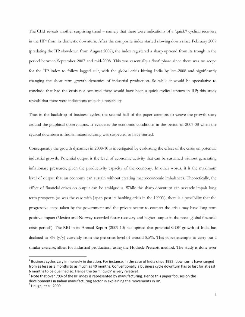
The CILI reveals another surprising trend – namely that there were indications of a „quick‟3 cyclical recovery

in the IIP4 from its domestic downturn. After the composite index started slowing down since February 2007

(predating the IIP slowdown from August 2007), the index registered a sharp uptrend from its trough in the

period between September 2007 and mid-2008. This was essentially a „lost‟ phase since there was no scope

for the IIP index to follow lagged suit, with the global crisis hitting India by late-2008 and significantly

changing the short term growth dynamics of industrial production. So while it would be speculative to

conclude that had the crisis not occurred there would have been a quick cyclical upturn in IIP; this study

reveals that there were indications of such a possibility.

Thus in the backdrop of business cycles, the second half of the paper attempts to weave the growth story

around the graphical observations. It evaluates the economic conditions in the period of 2007-08 when the

cyclical downturn in Indian manufacturing was suspected to have started.

Consequently the growth dynamics in 2008-10 is investigated by evaluating the effect of the crisis on potential

industrial growth. Potential output is the level of economic activity that can be sustained without generating

inflationary pressures, given the productivity capacity of the economy. In other words, it is the maximum

level of output that an economy can sustain without creating macroeconomic imbalances. Theoretically, the

effect of financial crises on output can be ambiguous. While the sharp downturn can severely impair long

term prospects (as was the case with Japan post its banking crisis in the 1990‟s); there is a possibility that the

progressive steps taken by the government and the private sector to counter the crisis may have long-term

positive impact (Mexico and Norway recorded faster recovery and higher output in the post- global financial

crisis period5). The RBI in its Annual Report (2009-10) has opined that potential GDP growth of India has

declined to 8% (y/y) currently from the pre-crisis level of around 8.5%. This paper attempts to carry out a

similar exercise, albeit for industrial production, using the Hodrick-Prescott method. The study is done over

3 Business cycles vary immensely in duration. For instance, in the case of India since 1995; downturns have ranged

from as less as 8 months to as much as 40 months. Conventionally a business cycle downturn has to last for atleast 6 months to be qualified so. Hence the term ‘quick’ is very relative! 4 Note that over 79% of the IIP index is represented by manufacturing. Hence this paper focuses on the

developments in Indian manufacturing sector in explaining the movements in IIP. 5 Haugh, et al. 2009

5

two periods of data – till 2009 and consequently till the present date (August 2010). The study shows an

interesting result – when data till 2009 is taken into consideration; potential output growth was seen declining

to 6.6% from its pre-crisis level of around 8.5%. However, when the entire period till August 2010 was taken

for analysis; the potential growth stood increased at around 9%. This underlines the inherent strength of the

recovery in the first eight months of 2010 that influenced the long term estimate of industrial growth so

strongly.

This paper bases its analysis on one of the concluding suggestions made by the Reserve Bank of India‟s

Technical Advisory group on Development of Leading Economic Indicators for the Indian Economy, 2006.

The group observed that, “Indian business cycles through the nineties are non-uniform.......Since change is rapid, particularly

in the last few years, it may be worthwhile to redo the identification exercise of leading indicators......focussing on the period 2000

onwards.” The group further noted that doing the exercise was beyond its scope then, since “In case the analysis

is carried out on the period 2000 onwards, we will have only 72 monthly and 24 quarterly observations6, which would be too few

to carry out meaningful business cycle analysis. Accordingly this exercise will be carried out over time as the number of

observations become sufficiently large.”

This paper has the opportunity to consider data till August 2010, hence significantly addressing RBI‟s

roadblock back in March 2006. While the business cycle in this paper has been constructed since 1995 in

order to portray a fuller picture of India‟s business cycle phases; the scope of this paper is beyond its simple

construction. The main aim remains analysing the movements specifically in the period beyond 2007 in which

the Indian business cycle faced one of its deepest slumps in recent history. Under the circumstances, RBI‟s

warning on using previous data is very germane to the inference of results, since running the econometric

procedures for constructing leading economic indicators using data from the nineties could possibly skew

results. So even though the growth cycle reveals only four major turning points in the period from 2000-2010;

it is crucial that the leading economic indicators take cognizance of these phases in particular. Hence in line

6 Since the study was done in 2006.

6

with RBI‟s recommendations, the composite leading economic indicator index has been constructed for the

period January 2000 - August 2010 and analysed with respect to the growth cycle specifically for this period.

This paper is divided in two broad halves. The first concerns itself with the mechanics of business cycles and

constructs a basic business cycle model and its corresponding leading economic indicator index. The second

half analyses the business cycles in tandem with the economic situation at that time.

In the first half; Section II talks about the basic theory of business cycles and the evolution of the business

cycle literature over the years. It will set the tone for the methodologies to be adapted in the paper.

Section III constructs the business cycle and leading economic indicator index and analyses the results.

Section IV studies the key phases of the contemporary business cycle. After a brief snapshot of the growth

phase in 2002-07, the paper studies the economic conditions prevailing in 2007-08, and how a slowdown was

imminent. Section V covers the period of the global financial crisis and consequent recovery. It analyses the

effect on potential industrial growth using the same computational methodology as the construction of

business cycles. Section VI concludes the main findings.

SECTION II

Business Cycle Theory:

Business Cycles represent periodicity of phases in expansion and contraction of economic activity. The

classical definition of business cycles as proposed by Burns and Mitchell7 (1946) is: “Business cycles are a type of

fluctuations found in the aggregate economic activity of nations that organize their work mainly in business enterprises: a cycle

consists of expansions occurring at about the same time in many economic activities, followed by similarly general recessions,

contractions and revivals which merge into the expansion phase of the next cycle; this sequence of changes is recurrent but not

periodic. In duration, business cycles vary from more than one year to ten to twelve years; they are not divisible into shorter cycles

7 From the National Bureau of Economic Research (NBER), founded in New York, 1920. Some of the earliest

research in this field has been initiated from here.

7

of similar character with amplitudes approximating their own.” This „traditional‟ concept highlights some important

characteristics of the business cycle, namely that it is a cycle of recessions followed by expansion and it

happens simultaneously in a number of economic variables. Further there is no particular consistency in the

periodicity of these cycles and that there needs to be processes in place to identify phases that are „long‟

enough to qualify as part of the business cycle.

However the concept of „aggregate economic activity‟ in the above definition has been debated in the

business cycle literature. The basic mechanism of business cycle is that a recession occurs when there is a

decline in some economic activity (regardless of what triggers it), and has a cascading effect on other

measures of activity. The transmission effect in the economy plays an important role in the creation of cycle.

However a transient decline in the absolute level of an aggregate measure like GDP may not necessarily

trigger falling incomes, sales and employment. Further in post-World War II, economies like Germany and

Japan registered sustained rise in GDP, which as per the classical definition would ignore key cycles in the

economy (Dua and Banerji, 1999).

Hence the concept of business cycle very often loosely accommodates what is described as a „growth‟ cycle

and „growth rate‟ cycle. A growth cycle traces expansion and contraction based on deviation of actual growth

rate from its long-run trend rate of growth. This is an improvement from the classical concept of business

cycle since a slowdown in a growth cycle signifies slowdown in economic activity as opposed to an absolute

decline. However this methodology has inherent complications like deseasonalisation and determination of

long term growth trend. Methods like Hodrick-Prescott Filter, Band Pass Filter or Phase-Average-Trend can

be used to for detrending purposes. The difficulties with the growth cycle approach led researchers to adapt

growth rate cycles. The „growth rate‟ cycle reflects cyclical movements in the growth rate of economic

activity. Usually year-on-year growth rates are preferred to month-on-month ones since the former are less

noisy. In order to lessen the noise in the series, one possible avatar of the growth rate used in literature is the

8

six-month smoothed growth rate. Growth rate cycles are generally used for real time monitoring and

forecasting, while growth cycles are said to be more suitable for historical analysis8.

For measurement of business cycles, it is necessary to observe a benchmark series known as the reference

series, which encompasses the overall economic activity. Such a series could be a single indicator or a

combination of certain economic series that fluctuate synchronously, also called a composite coincidental

indicators index. The latter may be preferred to reduce probability of false signals. Prima facie, GDP ought to

be taken as the reference series. However GDP also comprises of agricultural sector, which primarily depends

on rainfall and other climactic conditions and hence contributes to unwanted volatility in the index. It is

hence of popular practice to consider non-agricultural GDP as the reference series. The disadvantage of using

non-agricultural GDP is that in most cases, only quarterly figures are available. Tracking economic activities

at higher frequency is often required for a more complete analysis. Hence for the purpose of monthly data

analysis, Index of Industrial production is popularly used.

Finally the identification of cycles is very crucial since it cannot be expected that every series will have smooth

cyclical movements with clearly demarcated troughs and crests. There are several theories as to how the

identification is to be done. The most popular of them is the Bry-Boschan (1971) procedure, which suggests

the following rules for identification of cycles:

1. Peaks (troughs) are always followed by troughs (peaks)

2. The duration of an upswing and downswing regime is to be atleast six months.

3. The minimum length between any two alternating turning points (a cycle of peak to peak or trough

to trough) is 15 months to distinguish business cycles from seasonal cycles.

4. Turning points within 6-months of beginning or at the end of the time series are eliminated.

5. A turning point is the most extreme value between two adjacent regimes. If there are two or more

equal values satisfying the first three requirements, the most recent is chosen as the turning point of

the regime.

8 Klein, P.A. (1998)

9

CONSTRUCTING CYCLES

This paper uses the concept of growth cycles. For constructing growth cycles, it is necessary for the cyclical

component of the series to be extracted since by definition it traces the ups and downs in economic activity

through the deviation of actual growth rate from the long-run trend rate of growth. The series has to be

deseasonalised to rule out possible movements in the cycle due to seasonal factors. There are a number of

primitive as well as sophisticated methods developed to extract seasonality from data. One of the more

sophisticated methods is the Census Bureau methods developed by the US Bureau of the Census. Census II

has gone through several variations and refinements since 1955, when the first version was developed. The

most widely used variants have been X-11 (Shiskin, Young and Musgrave, 1967) and X-11 ARIMA (Dagum,

1988). The latest method available is the X-12 ARIMA methodology, which has been used in this paper9. The

broad concept remains to extract the seasonal and trend components using moving average methods

iteratively.

For detrending a series, the Hodrick-Prescott (HP) filter is used in this study. This methodology is popularly

used to extract the cyclical and trend components from time series. The filter basically amplifies the business

cycle frequencies and dampens short- and long- run variations. In the equation:

where Yt is the value of Y at time t and Tt stands for trend component at time t, the HP method chooses that

value of Tt that minimises the above function for a given value of λ. Note that (Yt – Tt) equates to the cyclical

component of a series and the above function is akin to a loss function that needs to be minimised. λ controls

the smoothness of the trend. For λ = 0, there is no penalty on the trend adjustment and the actual observed

series becomes the trend component. For monthly series, Serletis and Krause (1996) suggested λ to be equal

to 129600 for monthly series.

9 For a more complete discussion, Makridakis, Wheelwright, Hyndman, “Forecasting – Methods and Applications”,

3rd

Edition, Chapter 3.

10

Note that the HP filter has been used in two avatars in this paper. During the construction of business cycles

and composite leading economic indicator index, it has been used to extract the cyclical component of the

series. It is again used in Section IV and V where potential growth is calculated. Herein the power of the

method in extracting trend component of the series is exploited.

LEADING INDICATORS

There are broadly three types of indicators- leading, coincidental and lagging indicators. As the name suggests,

leading indicators are those economic series that predate the business cycle turns, hence „leading‟ the

reference series. For instance, capital goods index indicating investment level could point towards where

industrial production is likely to head. A leading economic indicator index is of particular interest in the study

of business cycles since it carries within it the power to forecast the peaks and troughs in the reference series.

A lagging indicator is one that reacts after the reference series has moved. Employment for instance could be

a lagging indicator, since hiring usually begins in reaction to good growth, instead of the reverse. However

economic reasoning can be fallacious and is not a full-proof way to decide on whether indicators are leading,

coincidental10 or lagging.

The selection of indicators forms a crucial exercise in business cycle analysis since the forecasting

performance of the index depends on it. The basic requirement of any indicator is that it needs to be an

economic variable that is of high significance and importance. Ideally it should have a high frequency of data

release – after all a data that is released annually will not be very receptive to monthly trends in the economy.

A leading indicator, as the name suggests, needs to be cognizant of future economic activity. Consistency of

the indicator is also a key determinant since it needs be checked how efficiently the indicator has predated the

reference series in the past and whether it has conformed to the business cycle patterns at large. Apart from

visual observation of the peaks and troughs of the two series, there are several other more complete ways to

check how well a potential indicator series „indicates‟ the reference series. In this paper, the method of cross-

10

Coincidental indicators move in tandem with the reference series.

11

correlation is used. Cross correlation between two variables checks how well one variable correlates with

different lags of the other variable. Cross correlation between the two series x and y is given by:

where l = 0, ±1, ±2,.......

and / T l = 0, 1, 2,...

= / T l = 0, -1, -2,...

If x is a good leading indicator then it will show the highest value of cross correlation with one of the lags (l)

of IIP; which will ascertain by how many periods the indicator is leading it. A higher value of l is preferred

since it means that the indicator with reach l periods before the reference series.

A variety of indicators need to be tested in this fashion and a collection of the most robust indicators need to

be combined into an index called the leading economic indicator index. It is preferred that the indicators be

chosen from all fields of economic activity to make the analysis comprehensive. The reason behind creating

an index is made to rule out the possibility of idiosyncratic behaviours in individual series. While there are

many methods available in literature for creating such an index, this paper uses the method of normalising the

cyclical component of all the indicators to unit mean and variance and then simply adding the standardized

cyclical components11. The standardization of the components helps in preventing the more volatile series

from dominating the combined index.

LITERATURE SURVEY

Esoteric to Indian business cycles, Chitre (1991) analysed 94 monthly time series for the period 1951 to 1982

and presented evidence of synchronous movements in respect of a number of key economic processes. Dua

and Banerji (2001) followed the classical NBER approach to estimate the reference chronologies of Indian

11

As done in Report of Technical Advisory Group on Development of Leading Economic Indicators for Indian Economy, RBI (2006)

12

business cycles and the growth rate cycles. The study focused on the approach for construction of composite

co-incident index; identified leading and coincident indicators, and dating business cycles. It was observed

that Indian business cycles have averaged over six years in length, with recessions averaging just less than a

year and expansions a little over five years. Hatekar (1993) used annual data for the period 1950-85 and tested

the real business cycle proposition that nominal magnitudes and real money balances cannot be exogenous

during mechanisms of the business cycle. Gangopadhyay and Wadhwa (1997) used monthly data on IIP for

the period Q2 1975 to Q1 1995 for obtaining the chronology of Indian business cycles using deterministic

trend. Mohanty et al. (2003) used monthly data of the Index of Industrial Production index and identified 13

business cycles in the economy with varying durations during 1970-71 to 2001-02. Mall (1999) characterized

Indian business cycles based on the non-agricultural GDP as the reference series. The turning points of IIP

Manufacturing were found to be roughly coincident with major output variables in the non-agricultural sector

of the economy. Shah and Patnaik (2010) have investigated macroeconomic stabilisation in the backdrop of

the Indian business cycle.

Moore in 1950 established, what could be the first list of leading indicators, comprising of - sensitive

commodity prices, average manufacturing workweek, commercial and industrial building contracts, new

incorporations, new orders, housing starts, stock price index, and business failure liabilities. The ECRI

maintains leading, coincidental and lagging indicators for twenty countries including India using real GDP as

the reference series; while the US Conference Board does it for nine major countries - the US, Australia,

France, Germany, Japan, Korea, Mexico, Spain and the UK. The Organization of Economic Cooperation and

Development (OECD) also tracks business cycles for twenty nine member countries and six non-member

countries The OECD CLI is based on the growth cycle approach. Their indicator system uses univariate

analysis to estimate trend and cycles individually for each component series and then a CLI is obtained by

aggregation of the resulting de-trended component. OECD (2006) has recently developed a Composite

Leading Economic Indicator for India. The RBI had initiated two studies on the construction of various

forms of business cycles and leading economic indicators; one in 2002 and the other in 2006. The study

details the processes of construction of growth and growth rate cycles with respect to quarterly non-

13

agricultural GDP and monthly IIP index. It also establishes guidelines for construction of the corresponding

composite leading indicator indices. This paper borrows much of its methodology from the guidelines

suggested in the 2006 study.

SECTION III

Business Cycle Analysis:

This paper uses the concept of growth cycles. Using the methods described in Section I, the cyclical

component of the Index of Industrial Production (IIP) is extracted and analysed for the identification of

business cycles. The deseasonalized and detrended series is smoothed using six-month moving average in

order to reduce the short-term irregular component. Though for the leading economic indicator index, the

paper follows RBI‟s recommendation of considering data 2000 onwards; Fig. 1 below is a snapshot of

business cycle formation since 1995.

-15

-10

-5

0

5

10IIP Growth Cycle (From 1995)

Fig 1

14

(Table. 1) Dating Cycles since 1995

PEAK TROUGH EXPANSION (Trough to Peak)

DOWNTURN (Peak to Trough)

CYCLE (Peak to Peak)

May-96 Feb-97 - 8 -

Nov-97 Mar-99 9 16 18

May-00 Aug-03 14 39 42

Dec-04 Dec-05 16 12 55

Aug-07 May-09 20 21 44

Average 15 19 40

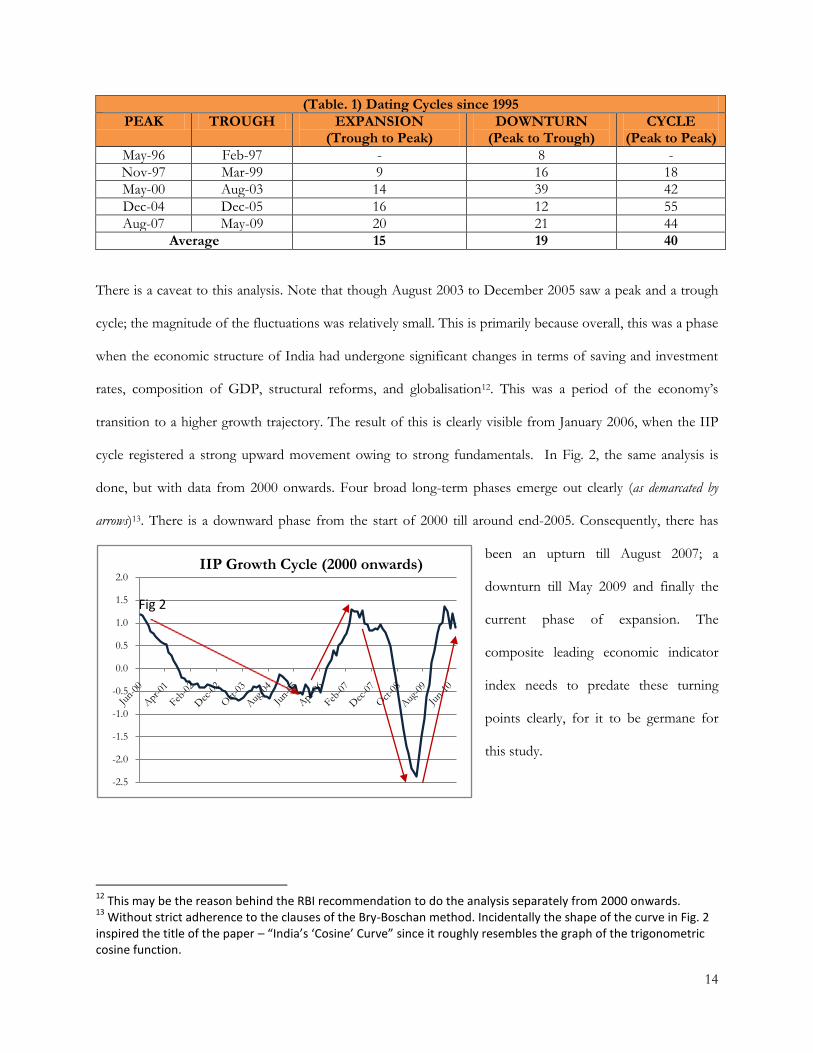
There is a caveat to this analysis. Note that though August 2003 to December 2005 saw a peak and a trough

cycle; the magnitude of the fluctuations was relatively small. This is primarily because overall, this was a phase

when the economic structure of India had undergone significant changes in terms of saving and investment

rates, composition of GDP, structural reforms, and globalisation12. This was a period of the economy‟s

transition to a higher growth trajectory. The result of this is clearly visible from January 2006, when the IIP

cycle registered a strong upward movement owing to strong fundamentals. In Fig. 2, the same analysis is

done, but with data from 2000 onwards. Four broad long-term phases emerge out clearly (as demarcated by

arrows)13. There is a downward phase from the start of 2000 till around end-2005. Consequently, there has

been an upturn till August 2007; a

downturn till May 2009 and finally the

current phase of expansion. The

composite leading economic indicator

index needs to predate these turning

points clearly, for it to be germane for

this study.

12

This may be the reason behind the RBI recommendation to do the analysis separately from 2000 onwards. 13

Without strict adherence to the clauses of the Bry-Boschan method. Incidentally the shape of the curve in Fig. 2 inspired the title of the paper – “India’s ‘Cosine’ Curve” since it roughly resembles the graph of the trigonometric cosine function.

-2.5

-2.0

-1.5

-1.0

-0.5

0.0

0.5

1.0

1.5

2.0IIP Growth Cycle (2000 onwards)

Fig 2

15

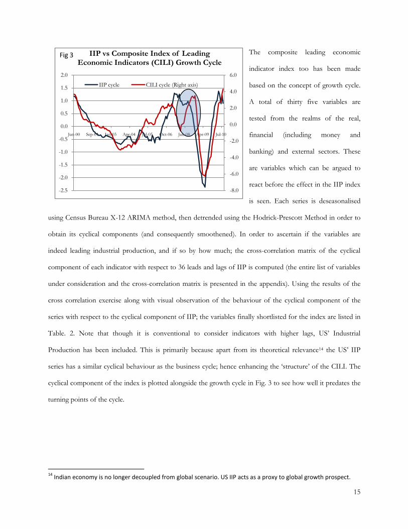
The composite leading economic

indicator index too has been made

based on the concept of growth cycle.

A total of thirty five variables are

tested from the realms of the real,

financial (including money and

banking) and external sectors. These

are variables which can be argued to

react before the effect in the IIP index

is seen. Each series is deseasonalised

using Census Bureau X-12 ARIMA method, then detrended using the Hodrick-Prescott Method in order to

obtain its cyclical components (and consequently smoothened). In order to ascertain if the variables are

indeed leading industrial production, and if so by how much; the cross-correlation matrix of the cyclical

component of each indicator with respect to 36 leads and lags of IIP is computed (the entire list of variables

under consideration and the cross-correlation matrix is presented in the appendix). Using the results of the

cross correlation exercise along with visual observation of the behaviour of the cyclical component of the

series with respect to the cyclical component of IIP; the variables finally shortlisted for the index are listed in

Table. 2. Note that though it is conventional to consider indicators with higher lags, US‟ Industrial

Production has been included. This is primarily because apart from its theoretical relevance14 the US‟ IIP

series has a similar cyclical behaviour as the business cycle; hence enhancing the „structure‟ of the CILI. The

cyclical component of the index is plotted alongside the growth cycle in Fig. 3 to see how well it predates the

turning points of the cycle.

14

Indian economy is no longer decoupled from global scenario. US IIP acts as a proxy to global growth prospect.

-8.0

-6.0

-4.0

-2.0

0.0

2.0

4.0

6.0

-2.5

-2.0

-1.5

-1.0

-0.5

0.0

0.5

1.0

1.5

2.0

Jun-00 Sep-01 Jan-03 Apr-04 Jul-05 Oct-06 Jan-08 Apr-09 Jul-10

IIP vs Composite Index of Leading Economic Indicators (CILI) Growth Cycle

IIP cycle CILI cycle (Right axis)

Fig 3

16

(Table. 2) Components of Leading Economic Indicator Index

VARIABLE LEAD MONTHS

Two wheelers‟ production 16

Railway earnings from goods traffic (Rs crore) 17

IIP- Consumer Durable Goods 16

Oil Imports (Rs crore) 7

US‟ IIP 3

There are several key points that emerge out in the analysis:

1. The CILI seems to have done a reasonably good job of predating the broad trends in the IIP cycle as

illustrated in Fig. 3. While the IIP cycle turned upward from around end-2005, the CILI started its

journey upwards a year earlier in mid-2003. Then the indicator peaks at February 2007, and the IIP

cycle followed suit in August 2007. Consequently the indicator falls till September 2007, which was

followed by the IIP cycle post-August 2007.

2. However there is period of sharp rise in the composite indicator cycle, from September 2007 to

July 2008 for which there is no corresponding upturn in the IIP cycle. The IIP cycle had already

peaked at May 2007 and was in its cyclical downturn in this period. The consequent upturn in the

leading indicator index could imply that there was a possibility of a cyclical recovery from that

downturn. This is quite plausible, since end-2007 was a period when the global economy was

growing strong and sentiments were high. By 2007, India‟s service sector was clocking over

10% (y/y) growth15 causing GDP to grow at over 9% for most of the quarters. Infact there was

increasing speculation of India crossing the double-digit growth mark. However there is no scope to

be certain that the IIP index would have reacted; since by end-2008 the global crisis struck India and

the growth story dramatically changed.

3. The global slowdown affected sharply both the IIP series and all its leading indicators (vehicle

production, railway freight, durable goods‟ production, imports, etc.). The shock caused both the

15

The leading economic indicators also include variables that are strongly influenced by service sector growth.

17

series sharply fell in the crisis period and the gap or „lead‟ that the indicator index enjoyed over the

reference series in the previous turning points collapsed with the crisis shock.

Thus the Business Cycle Analysis section concludes with there are three main phases that merit further

discussion. First is the period 2007-08, when the IIP cycle started showing slowdown. Next is the period

between 2008 and 2010, which was characterised by a sharp decline in the cycle, followed by a quick recovery.

Finally the period 2002-07 is interesting given that it was marked by sustained strengthening of the IIP cycle.

SECTION IV

Elucidating the Business Cycle:

SNAPSHOT OF GROWTH PHASE: 2002-07

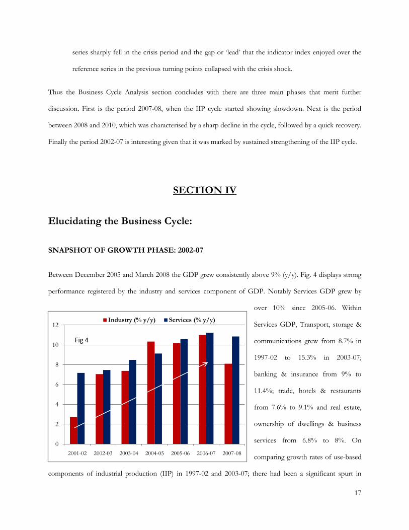
Between December 2005 and March 2008 the GDP grew consistently above 9% (y/y). Fig. 4 displays strong

performance registered by the industry and services component of GDP. Notably Services GDP grew by

over 10% since 2005-06. Within

Services GDP, Transport, storage &

communications grew from 8.7% in

1997-02 to 15.3% in 2003-07;

banking & insurance from 9% to

11.4%; trade, hotels & restaurants

from 7.6% to 9.1% and real estate,

ownership of dwellings & business

services from 6.8% to 8%. On

comparing growth rates of use-based

components of industrial production (IIP) in 1997-02 and 2003-07; there had been a significant spurt in

0

2

4

6

8

10

12

2001-02 2002-03 2003-04 2004-05 2005-06 2006-07 2007-08

Industry (% y/y) Services (% y/y)

Fig 4

18

capital goods (5.9% to 14.3%) and consumer non-durables (4.3% to 10.4%). Corporate performance in

terms of growth in net sales increased from an average of around 8% in 2002-03 to over 18% in 2007-0816.

In terms of investment levels; Gross fixed capital investment as percentage of GDP rose from an average of

25% in 2002-03 to 36% in 2007-08. This surge in investment has been largely financed by domestic resources.

This is evident from the growth in gross domestic savings - that increased from 7% (y/y) in 2001-02 to

around 21% in 2007-08. In particular, the growth in public sector savings has been remarkable – from a dis-

saving of Rs 36,000 crore in 2001, public sector savings grew to a surplus of around Rs 90,000 crore in 2006

and Rs 138,000 crore in 2007. Private sector earnings were not as dire as public savings in 2001. It rose by

around 300% in 2007 compared to 2001 levels. Though there had been an increased inflow of foreign private

capital, foreign capital‟s contribution to additions in fixed capital stock had been modest (Nagaraj 200817).

The surge of growth in this period could primarily be attributed to restructuring measures by domestic

industry; huge unmet domestic demand, especially in sectors like communication; introduction of newer

technologies; increased productivity owing to further liberalisation of the economy (software boom) and

strong global growth. Also this period experienced one of the longest credit cycles in recent past. Nominal

bank credit growth had accelerated to 38% (y/y) in March 2006 from the bottom of 10.7% in September

2003, supported primarily by a subdued interest rate regime in this period. A snapshot of the sectoral break-

up of the bank lending in this period in Table. 3 shows that the portfolio of outstanding housing loans as a

percentage of outstanding bank credit rose from 4.7% in 2001 to 9.7% in 2004 and 12% in 2007. The growth

in consumer durable loans is concealed in the table due to the small fraction it represents of the total loans

made by scheduled commercial banks. However in terms of incremental raise annually - consumer durables

loans made in 2006 were a whopping 118% higher than those disbursed in 2004. In all, growth in consumer

durable loans between 2004 and 2008 has been around 129%; in housing loans by 168% and in industry loans

by 121%!

16

Data based on Centre of Monitoring Indian Economy (CMIE)’s compilation of statistics for over 4000 companies. 17

Nagaraj, R. (2008), “India’s Recent Economic Growth: A Closer Look” Economic and Political Weekly, Vol. 43, No. 15, April 12, 2008, pp 55-61

19

(Table. 3) Percentage of total outstanding bank credit

2001 2004 2006 2007 2008

Industry 43.91 38.03 38.77 37.40 38.10

Personal 12.25 20.34 22.21 23.33 22.27

~Consumer Durables 0.64 0.48 0.55 0.44 0.49

~Housing 4.72 9.70 11.00 12.03 11.76 Compiled from Basic Statistical Returns, Reserve Bank of India

SLOWDOWN IN 2007-08

For a reliable way to gauge how well the industrial production has performed, it is necessary that it is

compared to a benchmark. The potential output growth rate can be used for such benchmarking purposes18.

Potential output is the level of economic activity that can be sustained without generating inflationary

pressures, given the productivity capacity. The output gap is the difference of actual output as compared to

the potential output. Calculating what the potential output ought to be has been a matter of considerable

debate in literature. This paper uses the popular method of Hodrick-Prescott Filter, which essentially

decomposes a series into its trend and cyclical components. For a considerably long data series, the extracted

trend gives a „rough‟ estimate for potential output. Herein we use data from May 1994 to August 2008 to

18

The topic of potential output and its reaction to the crisis is covered in detail in Section V

0

4

8

12

16

Jan

-00

May

-00

Sep

-00

Jan

-01

May

-01

Sep

-01

Jan

-02

May

-02

Sep

-02

Jan

-03

May

-03

Sep

-03

Jan

-04

May

-04

Sep

-04

Jan

-05

May

-05

Sep

-05

Jan

-06

May

-06

Sep

-06

Jan

-07

May

-07

Sep

-07

Jan

-08

May

-08

Actual IIP growth (% y/y) Potential output growth (% y/y) (Till Aug 2008)

Fig 5

20

arrive at the calculation for potential growth rate of IIP. Fig. 5 is however shown from 2000 onwards for

better representation purposes. The graph for the entire period is presented in the appendix.

Fig. 5 shows that there has been a distinct improvement in potential output in the period from 2002 to 2008

– growing from a little over 5% to above 8%. This implies increase in productive capacity in the industrial

sector. The trend seems to stabilize by 2006. Looking at the actual IIP growth, it is seen that till 2005, growth

was close to the long term trend. However post 2007; IIP growth fell below potential indicating that there

were signs of the cycle turning from its peak. From 14% (y/y) growth in IIP in March 2007, growth fell to

around 2% in August 2008. Manufacturing; that accounts for about 80% of industrial production fell by 9.6

percentage points in this period.

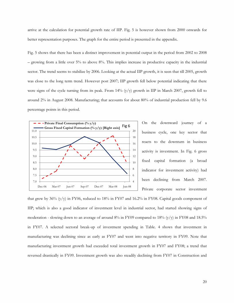
On the downward journey of a

business cycle, one key sector that

reacts to the downturn in business

activity is investment. In Fig. 6 gross

fixed capital formation (a broad

indicator for investment activity) had

been declining from March 2007.

Private corporate sector investment

that grew by 36% (y/y) in FY06, reduced to 18% in FY07 and 16.2% in FY08. Capital goods component of

IIP; which is also a good indicator of investment level in industrial sector, had started showing signs of

moderation - slowing down to an average of around 8% in FY09 compared to 18% (y/y) in FY08 and 18.5%

in FY07. A selected sectoral break-up of investment spending in Table. 4 shows that investment in

manufacturing was declining since as early as FY07 and went into negative territory in FY09. Note that

manufacturing investment growth had exceeded total investment growth in FY07 and FY08; a trend that

reversed drastically in FY09. Investment growth was also steadily declining from FY07 in Construction and

4

6

8

10

12

14

16

18

20

7.0

7.5

8.0

8.5

9.0

9.5

10.0

10.5

11.0

Dec-06 Mar-07 Jun-07 Sep-07 Dec-07 Mar-08 Jun-08

Private Final Consumption (% y/y)

Gross Fixed Capital Formation (% y/y) [Right axis]Fig 6

21

Social & Personal Services. Note that the remarkably bad performance seen in the last row of the table

(FY09) was accentuated by falling business sentiments during the global financial crisis.

(Table. 4) Selected Sectoral Break-up of Investment Spending

% y/y Gross Fixed

Capital Formation

Agricul-ture

Manufac-turing

Electricity, Gas and Water Supply

Construc-tion

Mining Transport, Storage and Commun-

ication

Social & Personal Services

FY06 16.04 18.10 14.84 28.64 0.66 40.05 14.65 18.00

FY07 16.10 1.37 25.52 23.67 45.52 3.47 0.96 12.31

FY08 15.21 16.53 19.77 8.69 23.49 14.63 26.33 16.39

FY09 -2.42 25.99 -21.88 1.29 -22.85 -7.79 30.35 6.20 Economic Survey, 2008-09

Consumption indicators too were showing slowdown in business cycle. Private Final Consumption

Expenditure growth was declining from December 2007 as displayed in Fig. 6. Consumer goods production

growth reduced from an average of 10.2% (y/y) in FY07 to an average of 6.2% in FY08. This has been

primarily driven by the durables sector that registered phases of negative growth in this period (Fig. 7).

Consumer durables, by concept represent a segment that is relatively income-elastic. Item-wise

decomposition of consumer durables shows weakening in Tractors, Tractor tyres, Two wheelers, Two

wheeler tyres, and to some extent passenger cars. Most of these items depend on availability of consumer

credit; and it could be possible that the effect of monetary tightening of the RBI in this period may have

caused the slowdown19. It needs to be taken into account that the phase of growth between 2002-2007 was

during a long upward phase of the credit cycle.

There could be a variety of reasons of what could have contributed to the slowdown. Globally, financial

markets were exhibiting volatility over concerns of a potential sub-prime crisis in the US. IMF‟s World

Economic Outlook (January 2008) forecasted global GDP to slow down from 4.9% in 2007 to 4.1% in 2008.

US‟ GDP fell from 2.7% (y/y) in Q4 2007 to 1.2% in Q2 2008; while EU‟s GDP fell from 2.2% to 1.2% in

the same period. Being a largely domestic driven economy, the effect of this moderation on India was

19

However there is a caveat to this analysis- the IIP - consumer goods series includes archaic items like Alarm clock, Tape Recorders and Typewriters which registered highly negative growth rates (as much as -88% (y/y)!) during this period. Hence the decline in consumer durables needs to be taken with a pinch of salt.

22

relatively mute. Infact merchandise exports of India averaged a healthy 27.4% (y/y) in 2007-08, and grew by

as much as 68% (y/y) in April 2008.

However the Indian economy was affected by the sharp increase in global commodity and crude oil prices.

While domestic prices of petrol and diesel witnessed a one-off upward adjustment in February 2008 (3-4 %),

after a gap of almost a year; non-administered petroleum products prices increased by around 39-42% with

international crude prices. Domestic iron and steel prices increased, reflecting higher domestic demand as

well as firm global prices. As a result overall domestic inflation (WPI) reached a high of 11.2% (y/y) in

August 2008 (according to the newly constructed 2004-05 base. As per the base of 1993-94 prevalent at that time, inflation

was much higher at 12.8%). While the RBI kept the LAF rates constant throughout 2007-08, it increased the

cash reserve ratio by 150 basis points. As Fig. 7 displays, the 10 year GSec yield had risen sharply by mid-

2008. The high commodity prices and interest rate regime would have created a dampening effect on business

sentiment. As Fig. 8 shows, index of RBI‟s Industry Outlook Survey20 on „Overall Business Situation‟ and

„Profit Margin‟ was declining from as early as June 2007; over a year before the global financial crisis

occurred.

20

Includes non-financial private and public limited companies engaged in manufacturing. The data is released quarterly.

7.0

7.5

8.0

8.5

9.0

9.5

-9

-6

-3

0

3

6

9

12

15

18

21

Nov-05 Jun-06 Jan-07 Aug-07 Mar-08

Consumer Goods-IIP (% y/y) 3 month MA

Non-durables

Durables

10 year Gsec Yield (Right axis)

Fig 7

-6

-4

-2

0

2

4

6

8

10

12

14

10

15

20

25

30

35

40

45

50

55

60

Mar-06 Sep-06 Mar-07 Sep-07 Mar-08 Sep-08 Mar-09

Overall Business SituationProfit Margin (Right axis)

RBI's Industrial Outlook Survey

Fig 8

23

SECTION V

The Global Financial Crisis, 2008-10:

EFFECT ON POTENTIAL INDUSTRIAL GROWTH

Potential output is the level of economic activity that can be sustained without generating inflationary

pressures, given the productivity capacity. Theoretically, financial crises ought to affect the output of the

economy by hurting consumption, investments and business sentiments. A persistent crisis could lead to a

sharp fall in investment and cause an output gap that may severely impair potential output; as was the case

with Japan post its banking crisis in the 1990‟s. Also crises have the potential to hurt productivity from

reduced capital spending and poor labour market conditions. Policy actions can lead to market distortions

that can prove to be long term bane. Whether such effects of a crisis will remain temporary or whether the

slowdown will have long-term implications, is a question that has considerable policy implications. However

it is not always the case that the long-term effects of a crisis may be negative. The aggressive policy responses,

structural reform and private sector restructuring could possibly have a positive influence long term output.

For instance, increased social sector spending or infrastructural investment undertaken during the crisis to

stimulate demand could help build potential output.

Some work on this subject has already been done in recent past. Furceri and Mourougane (2009) did an

empirical study on OECD countries over the period 1960-2007 to conclude that financial crises are estimated

to lower the potential output by an average of around 1.5-2.4%. On similar lines, Carra and Saxena (2008)

studies the output behaviour in 190 countries and found large, persistent actual output losses associated with

financial crises, with output falling by 7.5% relative to the trend over a period of ten years in the event of a

banking crisis. Park Cyn-Young, et al (2010) used various methods to investigate the post-crisis behaviour of

potential output in emerging East Asian economies and concluded that here was no or negligible potential

growth reductions in the case of China, Indonesia, and India.

24

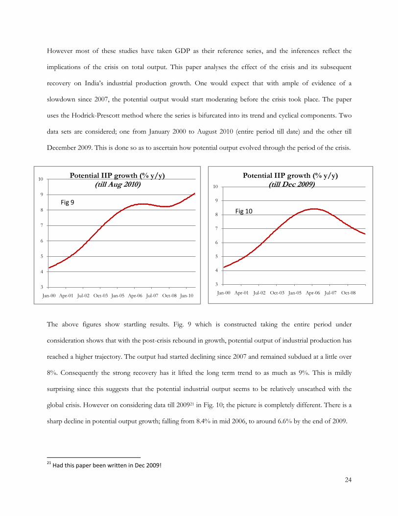
However most of these studies have taken GDP as their reference series, and the inferences reflect the

implications of the crisis on total output. This paper analyses the effect of the crisis and its subsequent

recovery on India‟s industrial production growth. One would expect that with ample of evidence of a

slowdown since 2007, the potential output would start moderating before the crisis took place. The paper

uses the Hodrick-Prescott method where the series is bifurcated into its trend and cyclical components. Two

data sets are considered; one from January 2000 to August 2010 (entire period till date) and the other till

December 2009. This is done so as to ascertain how potential output evolved through the period of the crisis.

The above figures show startling results. Fig. 9 which is constructed taking the entire period under

consideration shows that with the post-crisis rebound in growth, potential output of industrial production has

reached a higher trajectory. The output had started declining since 2007 and remained subdued at a little over

8%. Consequently the strong recovery has it lifted the long term trend to as much as 9%. This is mildly

surprising since this suggests that the potential industrial output seems to be relatively unscathed with the

global crisis. However on considering data till 200921 in Fig. 10; the picture is completely different. There is a

sharp decline in potential output growth; falling from 8.4% in mid 2006, to around 6.6% by the end of 2009.

21

Had this paper been written in Dec 2009!

3

4

5

6

7

8

9

10

Jan-00 Apr-01 Jul-02 Oct-03 Jan-05 Apr-06 Jul-07 Oct-08

Potential IIP growth (% y/y)(till Dec 2009)

Fig 10

3

4

5

6

7

8

9

10

Jan-00 Apr-01 Jul-02 Oct-03 Jan-05 Apr-06 Jul-07 Oct-08 Jan-10

Potential IIP growth (% y/y) (till Aug 2010)

Fig 9

25

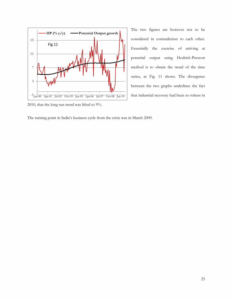
The two figures are however not to be

considered in contradiction to each other.

Essentially the exercise of arriving at

potential output using Hodrick-Prescott

method is to obtain the trend of the time

series, as Fig. 11 shows. The divergence

between the two graphs underlines the fact

that industrial recovery had been so robust in

2010, that the long run trend was lifted to 9%.

The turning point in India‟s business cycle from the crisis was in March 2009.

-1

3

7

11

15

Jan-00 Apr-01 Jul-02 Oct-03 Jan-05 Apr-06 Jul-07 Oct-08 Jan-10

IIP (% y/y) Potential Output growth

Fig 11

26

SECTION VI

Conclusion:

The aim of this study had been to identify where the global financial crisis fitted in the larger picture of

India‟s business cycle. In the process, this paper contributes to the existing literature on Indian business

cycles, by identifying the cycles from 1995-2010 (till August). The study is complimented by the construction

of a composite leading economic indicator index; which has been done using data from 2000 onwards. This

has been done in order to best capture the changing dynamics of Indian growth, as recommended by the

Reserve Bank of India‟s Technical Advisory group for Development of Leading Economic Indicators for the

Indian Economy (2006). Hence it is by and large the most up-to-date analysis conducted on Indian business

cycles so far. The growth cycle for India‟s industrial production was constructed using the Index of Industrial

Production index as the reference series and the turning points were identified using the Bry-Boschan

methodology. The study showed that the cycle had started its downturn from as early as August 2007,

indicating a domestic industrial downturn before the global financial crisis. The paper analyses in detail the

period of 2007-08 and finds that this inference is indeed corroborated by the economic situation prevailing at

that time.

The second finding of the paper is that there was an indication of a „quick‟ recovery from the aforesaid

cyclical downturn. This inference has been made by observing the composite leading economic indicator with

reference to the growth cycle. This indicator has been constructed taking the cyclical components of two

wheelers‟ production; railway earnings from goods traffic; oil imports, IIP-Consumer Durables index and US‟

IIP. After registering a downturn in the period from February 2007 (hence predating the cyclical downturn),

the leading index started showing a sharp upturn from September 2007 to July 2008. This movement could

have indicated that a recovery from the cyclical downturn was on the offing. However there is no scope to

confirm this since in end-2008, the global crisis struck India and the growth story dramatically changed.

27

Next the paper tries to weave India‟s growth story around the observations made in the business cycle study.

There is a short note on the growth phase between 2002 and 2007. Next the paper covers the period of

slowdown in 2007-08; which the analysis claims to have been the time when the downturn actually started.

Finally the paper covers the period of 2008-10; when the financial crisis and consequent recovery occurred. In

an effort to display the strength of the recovery; this paper investigates the effect of the crisis on potential

industrial growth. Potential output is the level of economic activity that can be sustained without generating

inflationary pressures, given the productivity capacity of the economy. Theoretically, the effect of financial

crises on output is equivocal. While the sharp downturn can severely impair long term prospects (as was the

case with Japan post its banking crisis in the 1990‟s); there is a possibility that the progressive steps taken by

the government and the private sector to counter the crisis may have long-term positive impact. Most of the

existent literature has studied this question, albeit measuring potential output in terms of GDP. In the case of

India, potential IIP growth in pre-crisis situation was found to be around 8.5% (as of August 2008). This long

term trend had been reached after steady rise from 2001, when it was around 4%. When the potential growth

was recalculated to include the global crisis period (i.e. data taken till December 2009), it registered a sharp

decline, falling to 6.6% by the end of 2009. However the surprising revelation is that when the entire period

from 2000 to 2010 (till August 2010) was taken into consideration; the potential industrial growth was seen to

actually increase and currently stands at around 9%. This underlines the robustness of the recovery that

happened in 2010, which raised potential growth so strongly.

28

References:

Abiad, A.; R. Balakrishnan; P.K. Brooks; D. Leigh; and I. Tytell. 2009. What's the Damage?

Medium-term Output Dynamics After Banking Crises. International Monetary Fund Working Paper No.

09/245.

Archibugi, D. and A. Coco. 2005. Measuring technological capabilities at the country level: A survey and a

menu for choice. Research Policy. 34(2). pp. 175-194.

Artis, M; Bladen- Hovell, R.C.; Osborn, D.R.; Smith, G. and Zhang, W. (1995), "Predicting turning

points in the U.K. Inflation Cycle", The Economic Journal, Vol. 105, 1145- 1164.

Asian Development Bank. 2007. Ten Years After the Crisis: The Facts about Investment and Growth. In

Beyond the Crisis: Emerging Trends and Challenges. Manila.

Bautista, C. C. 2003. Estimates of output gaps in four Southeast Asian countries. Economics Letters. 80(3).

pp. 365-371.

Baxter, M. and King. R.G. 1999. Measuring Business Cycles: Approximate Band-Pass Filters for Economic

Time Series. Review of Economics and Statistics. 81(4). pp. 575-593.

Bhaskaran, M. and Ghosh, R. 2010 “Impact and Policy Responses India” prepared for Asian Development

Bank, ADB Regional Forum on the Impact of Global Economic and Financial Crisis. Manila, Phiippines.

Bikker, J.A. and Kennedy, N.O. (1999), "Composite Leading Indicators of Underlying Inflation of Seven EU

Countries", Journal of Forecasting, Vol.18, 225- 258.

Birchenhall, C.R., Jessan, Osborn, D.R. and Simpson, C. (1999), "Predicting U.S. Business Cycle

Regimes", Journal of Business and Economic Statistics, Vol. 17(3), 313-323.

Bry, G. and Boschan, C. (1971), "Cyclical Analysis of Time Series: Selected Procedures and Computer

Programs", National Bureau of Economic Research, Technical Paper No. 20.

29

Burns, A.F. and Mitchell, W.C. (1946), Measuring Business Cycles, National Bureau of Economic Research,

New York.

Cabrero, A. and Delriue, J.C. (1996), "Construction of a Composite Indicator for Predicting Inflation in

Spain", Document de Trabajo No. 9619, Banque de Espana - Servicio de Estudios.

Cerra, V. and Saxena, S.C. (2005). “Did Output Recover from the Asian Crisis? International Monetary

Fund Staff Papers”. 52(1). pp. 1-23.

Chandrasekhar, C.P. (2009). “‟The Costs of “Coupling‟: The Global Crisis and the Indian Economy”. Third

World Network Global Economy Series No. 19, Financial Crisis and Asian Developing Countries.

Chitre, V. (2001), "Indicators of Business Recessions and Revivals in India: 1951 -1982", Indian Economic

Review, Vol. XXXVI (1), 79- 105.

Clark, P.K. (1987). The cyclical component of U.S. economic activity. The Quarterly Journal of

Economics. 102(4). pp. 797-814.

Dua, P. and Banerji, A, (2000), "An Index of Coincident Economic Indicators for the Indian Economy,"

Working papers 73, Centre for Development Economics, Delhi School of Economics.

______________________(2001a), "An Indicator Approach to Business and Growth Rate Cycles: The Case

of India", Indian Economic Review, Vol. XXXVI(1), 55- 78.

______________________(2001b), "A Leading Index for the Indian Economy," Working papers 90, Centre

for Development Economics, Delhi School of Economics.

______________________(2001c), “Business Cycles in India”, Working Paper No. 146, Centre for

Development Economics, Delhi School of Economics.

De Leeuw, F.(1991), "Towards a Theory of Leading Indicators", in Leading Economic Indicators- New

Approaches and Forecasting Records, Eds. K. Lahiri and G. Moore, Cambridge University Press, 15-56.

30

Diebold, F.X. and Rudebusch G.D. (1999), Business Cycle - Durations, Dynamics and Forecasting, Princeton

University Press.

Estrella, A. and Mishkin, F. (1996) "Predicting U.S. Recessions: Financial Variables as Leading Indicators",

Federal Reserve Bank of New York Research Paper, No. 9609.

Furceri, D. and Mourougane, A. (2009), “The Effect of Financial Crises on Potential Output: New Empirical

Evidence From OECD Countries,” Economic Department Working Paper, No. 699, Organization of

Economic Co-operation and Development.

Gangopadhyay, S. & Wadhwa, W. (1997), “Leading Indicators for Indian Economy, Report by Ministry

of Finance & SERFA”, New Delhi

Gaudreault, C. and Lamy, R. (2002), "Forecasting a One Quarter Decline in Canadian Real GDP with Probit

Models", Department of Finance, Economic and Fiscal Policy Branch Working Paper, No. 6.

Hamilton, J.D. (1989), "A New Approach to the Economic Analysis of Non-stationary Time Series and the

Business Cycle", Econometrica, Vol. 57(2), 357- 384.

Hatekar, N. (1993),"Studies in Theory of Business Cycles (with special emphasis on Real Business Cycles

and their Applications to the Indian Economy, Ph.D.dissertation, University of Bombay.

Haugh, D., Ollivaud, P. and Turner, D. (2009), “The Macroeconomic Consequences of Banking Crises in

OECD Countries,” OECD Working Paper No 683, Organization of Economic Co-operation and

Development.

Klein, P.A. (1998), "Swedish Business Cycles - Assessing the Recent Records", Working Paper 21, Federation

of Swedish Industries, Stockholm.

Lamy, R. (1998), "Forecasting Canadian Recession with Macroeconomic Indicators", Finance Canada

Working Paper, No. 1.

31

Mall, O.P. (1999), "Composite Index of Leading Indicators for Business Cycles in India", RBI Occasional

Papers, Vol. 20, No.3, 373- 414.

Mensah, J.A. and Tkacz, G. (1998), "Predicting Canadian Recessions Using Financial Variables: A Probit

Approach", Bank of Canada Working Paper, No. 5.

Ministry of Finance Economic Division, Government of India (2008), “Economic Survey 2007-08”

______________________________________________ (2009), “Economic Survey 2008-09”

______________________________________________ (2010), “Economic Survey 2009-10”

Nagaraj, R. (2008), “India‟s Recent Economic Growth: A Closer Look” Economic and Political Weekly, Vol.

43, No. 15, April 12, 2008, pp 55-61

OECD (2006a), "Composite Leading Indicators for Major OECD non-members Economies", OECD

Statistics Working Paper, STD/DOC(2006)1.

______ (2006b), "Composite Leading Indicators for Major OECD non-members Economies", Short-term

Economic Statistics Division.

Park, C., Majuca, R., Yap, J., (2010) “The 2008 Financial Crisis and Potential Output in Asia: Impact and

Policy Implications.”, ADB Working Paper Series on Regional Economic Integration, No. 45, April

Qi, M. (2001), "Predicting US Recessions with the Leading Indicators via Neural Network Models",

International Journal of Forecasting, Vol. 17. No.3, 383-401.

Reddy, Y.V. (2007), “Some Perspectives on the Indian Economy”, RBI Bulletin, November.

Reserve Bank of India (2002), "Report of the Working Group on Economic Indicators".

_________________ (2006), “Report of Technical Advisory Group on Development of Leading Economic

Indicators for Indian Economy”.

32

________________ (2010), “Report on Currency and Finance 2008-09”.

________________ (2008), “Annual Report 2007-2008”

________________ (2009), “Annual Report 2008-2009”

________________ (2010), “Annual Report 2009-2010”

Serletis, A. and Krause, D. (1996), "Nominal stylised facts of US Business Cycles", Federal Reserve Bank of

St. Louis Review, 78(4), 49- 54.

Simone, A. (2001), "In search of Coincident and leading Indicators of Economic Activity in Argentina", IMF

Working Paper No. 30.

Silver, S.J. (1991), "Forecasting Peaks and Troughs in the Business Cycle: On the Choice and Use of

Appropriate Leading Indicator Series", in Leading Economic Indicators- New Approaches and Forecasting

Records, Eds. K. Lahiri and G. Moore, Cambridge University Press, 183- 195.

Stock, J.H. and Watson, M.W. (1991), "A probability model of the coincident economic indicators", in

Leading Economic Indicators: New approaches and Forecasting Records, Eds. K. Lahiri and G.H. Moore,

63- 89.

Subbarao, D. (2009a) “Global Financial Crisis: Questioning the Questions.” RBI Bulletin, August

__________ (2009b) “Impact of the global financial crisis on India – collateral damage and response.”,

Speech at the Symposium on “The Global Economic Crisis and Challenges for the Asian Economy in a

Changing World” organized by the Institute for International Monetary Affairs, Tokyo, 18th February.

__________ (2010) “India and the Global Financial Crisis Transcending from Recovery to Growth”,

Peterson Institute for International Economics, Washington DC, 26th April.

33

APPENDIX

1. Potential vs Actual industrial growth (Aug-1995 to Aug-2008)

2. List of indicators used

From the real sector:

1. Aluminium production (tonnes)

2. Cement production (lakh tonnes)

3. Commercial vehicle production

4. Utility vehicle production

5. Passenger cars production

6. Two wheelers production

7. Total vehicle production (sum of 3,4,5 and 6)

8. IIP Capital goods

9. IIP Consumer durable goods

10. IIP Consumer non-durable goods

11. IIP Basic goods

12. Port- Total commodity traffic („000 tonnes)

13. Railway traffic earnings from goods (Rs crore)

14. Wholesale Price Index

-2

2

6

10

14

18

Aug-95 Nov-96 Feb-98 May-99 Aug-00 Nov-01 Feb-03 May-04 Aug-05 Nov-06 Feb-08

Actual IIP growth (% y/y) Potential output growth (% y/y)

Potential Ouput vs Actual Output: Aug 1995 - Aug 2008

34

From the money and financial sector:

1. SENSEX level

2. Nifty level

3. FII inflows (Rs crore)

4. Aggregate Deposits (Rs crore)

5. M1 (Narrow money)

6. M3 (Broad money)

7. Total credit (Rs crore)

8. Non-food credit (Rs crore)

9. USD/INR (Rupee)

10. One month rupee forward

11. Three month rupee forward

12. 10 year GSec yield (%)

13. Real interest rate (10 year GSec yield – WPI)

14. Total cheque collection (Rs crore)

From the external sector:

1. Exports (USD million)

2. Imports (USD million)

3. Oil Imports (USD million)

4. Non-oil imports (USD million)

5. US Industrial Production

6. China Imports

7. Crude Oil price (IMF World Petroleum Average Crude Price in USD per Barrel)

35

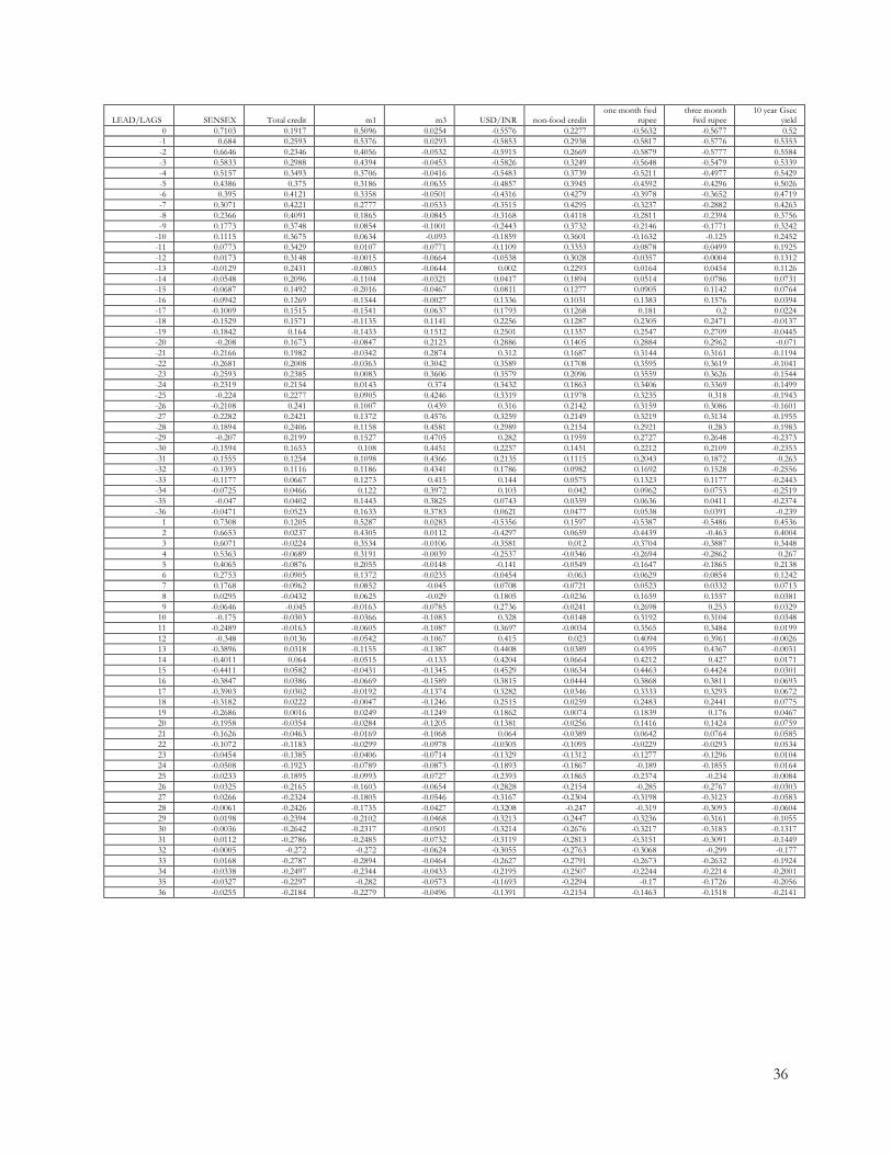
3. Cross-correlation matrix of indicators with IIP

LEAD/LAGS Cement Total vehicles Rail Port IIP - Durables IIP –

Nondurables IIP-

Intermediate Nifty FII

0 0.1796 0.5596 0.2021 0.4359 0.4789 0.3559 0.7368 0.6996 0.1212

-1 0.0131 0.4001 0.1002 0.3107 0.3678 0.1707 0.6122 0.6716 0.0623

-2 -0.0103 0.3241 0.1758 0.3987 0.2809 0.2603 0.5385 0.6585 0.0944

-3 -0.1001 0.2463 0.1399 0.307 0.2319 0.1787 0.4374 0.5783 -0.0046

-4 -0.1269 0.1895 0.1495 0.2787 0.1686 0.232 0.3933 0.5127 -0.0417

-5 -0.0967 0.1704 0.1064 0.2332 0.1076 0.1221 0.2975 0.441 -0.1907

-6 -0.176 0.0513 0.1206 0.1841 0.0097 0.1721 0.191 0.4014 -0.0932

-7 -0.2039 -0.0227 0.1153 0.1746 -0.0392 0.1485 0.138 0.315 -0.1747

-8 -0.1882 -0.1726 0.1182 0.1196 -0.1502 0.1939 0.0309 0.2427 -0.2176

-9 -0.1518 -0.2337 0.211 0.1699 -0.2215 0.2339 -0.0347 0.1875 -0.2354

-10 -0.1958 -0.3408 0.227 0.1064 -0.2662 0.2618 -0.1262 0.1206 -0.1864

-11 -0.1654 -0.3694 0.3245 0.1427 -0.32 0.2824 -0.1445 0.0921 -0.2563

-12 -0.1817 -0.4346 0.2826 0.1341 -0.3754 0.1989 -0.2332 0.0294 -0.2051

-13 -0.1145 -0.4499 0.3985 0.145 -0.4057 0.3131 -0.2229 -0.0016 -0.1601

-14 -0.0589 -0.5023 0.3646 0.1742 -0.4165 0.2276 -0.253 -0.0523 -0.2605

-15 0.0266 -0.5412 0.3893 0.2194 -0.4739 0.2643 -0.2944 -0.0613 -0.194

-16 0.0386 -0.51 0.4001 0.1951 -0.4818 0.1547 -0.3316 -0.0913 -0.2248

-17 0.007 -0.4754 0.401 0.1819 -0.415 0.2059 -0.322 -0.1003 -0.1887

-18 0.0996 -0.4517 0.3542 0.1365 -0.4174 0.1405 -0.303 -0.1523 -0.2561

-19 0.103 -0.4415 0.3146 0.0718 -0.3845 0.1262 -0.3045 -0.1871 -0.2443

-20 0.1243 -0.39 0.3066 0.0896 -0.3513 0.1 -0.28 -0.2119 -0.2186

-21 0.1318 -0.3402 0.2458 0.0094 -0.2896 0.1101 -0.2811 -0.2194 -0.1378

-22 0.1506 -0.2809 0.2385 -0.0242 -0.252 0.0522 -0.2277 -0.2734 -0.2294

-23 0.1504 -0.2279 0.1492 -0.0802 -0.1986 -0.0104 -0.1981 -0.2652 -0.0758

-24 0.1661 -0.1681 0.1733 -0.0899 -0.17 -0.0302 -0.1812 -0.2326 -0.0256

-25 0.1697 -0.1286 0.113 -0.0736 -0.103 -0.1279 -0.1576 -0.2237 0.005

-26 0.1448 -0.0631 0.106 -0.151 -0.0713 -0.1137 -0.0945 -0.2087 -0.0292

-27 0.1739 -0.0253 0.0576 -0.1416 -0.0606 -0.1448 -0.042 -0.2318 -0.0924

-28 0.1061 -0.0207 0.0578 -0.2011 -0.0108 -0.0829 -0.0144 -0.1904 0.0806

-29 0.0821 -0.0322 0.0182 -0.1807 -0.0171 -0.1561 0.0266 -0.21 0.0223

-30 0.0686 -0.0337 -0.0208 -0.2105 -0.0023 -0.1088 -0.0031 -0.1554 0.1271

-31 0.0432 -0.0101 0.0166 -0.1517 -0.004 -0.0894 0.0386 -0.1597 0.0555

-32 0.091 0.0491 -0.0324 -0.2086 0.0648 -0.1238 0.0877 -0.1369 0.0655

-33 0.0943 0.0623 -0.046 -0.1536 0.0429 -0.1722 0.108 -0.1152 0.0808

-34 0.0501 0.0965 -0.1104 -0.1401 0.0675 -0.2028 0.132 -0.0697 0.1479

-35 0.0398 0.1086 -0.0873 -0.1342 0.0733 -0.2124 0.1519 -0.043 0.1103

-36 0.0293 0.1718 -0.1496 -0.1741 0.1327 -0.2224 0.1674 -0.0439 0.1052

1 0.1198 0.4725 0.1599 0.3815 0.404 0.1777 0.6549 0.713 0.3107

2 0.241 0.4703 0.1772 0.3334 0.4108 0.0999 0.6882 0.6454 0.1923

3 0.1518 0.4021 0.1352 0.2737 0.4253 0.0686 0.6322 0.5866 0.351

4 0.2065 0.4007 0.1574 0.1746 0.408 0.1001 0.5597 0.5147 0.4249

5 0.2789 0.3138 0.1203 0.1522 0.3672 0.0672 0.4407 0.3807 0.3072

6 0.2661 0.2685 0.0246 0.1264 0.3189 -0.0348 0.355 0.248 0.3322

7 0.2741 0.2074 -0.1014 -0.0137 0.3211 -0.0013 0.2473 0.1495 0.4117

8 0.2454 0.1779 -0.1573 -0.0788 0.2848 -0.1093 0.1702 -0.0003 0.2457

9 0.1828 0.115 -0.1334 -0.1225 0.237 -0.1002 0.0482 -0.0904 0.2815

10 0.1461 0.1331 -0.2067 -0.187 0.2281 -0.1865 -0.0856 -0.1998 0.1734

11 0.2689 0.1014 -0.0917 -0.1705 0.2145 -0.0911 -0.1465 -0.2683 0.1252

12 0.1456 0.043 -0.1852 -0.2433 0.1753 -0.1216 -0.287 -0.369 0.0695

13 0.1938 0.0737 -0.1591 -0.2303 0.1288 -0.076 -0.3367 -0.4147 -0.0335

14 0.088 0.0399 -0.228 -0.2605 0.1125 -0.0743 -0.4354 -0.4173 0.0457

15 0.0727 0.0901 -0.1172 -0.1801 0.1335 -0.092 -0.4118 -0.4561 -0.1563

16 0.0515 0.0442 -0.0112 -0.189 0.0695 -0.0852 -0.4687 -0.3923 -0.1129

17 0.0293 0.1063 -0.0358 -0.1487 0.088 0.0027 -0.4352 -0.3961 -0.2427

18 -0.0482 0.0449 0.0316 -0.132 0.0708 0.0777 -0.439 -0.3144 -0.2169

19 -0.0331 0.0449 0.0667 -0.0691 0.0304 0.0262 -0.4403 -0.2585 -0.27

20 -0.0719 0.0683 0.0573 -0.0216 0.0273 0.0315 -0.3666 -0.1813 -0.1603

21 -0.0559 0.0196 0.0578 -0.0015 -0.0181 -0.0357 -0.3035 -0.1442 -0.1592

22 0.0059 0.0428 0.1138 0.0122 0.0043 0.0295 -0.2208 -0.0808 -0.2096

23 -0.1447 0.0016 0.082 0.0462 -0.0504 0.0192 -0.26 -0.0216 -0.0808

24 -0.0255 -0.0355 0.0494 0.0526 -0.062 -0.0318 -0.1642 -0.018 -0.1172

25 -0.1186 -0.0645 -0.0198 0.0634 -0.0827 -0.0673 -0.1469 0.0136 -0.0812

26 -0.0592 -0.0754 0.0104 0.084 -0.1228 0.0102 -0.0843 0.068 0.0503

27 -0.1003 -0.0967 -0.0629 0.1238 -0.1421 0.0286 -0.0457 0.0576 0.0463

28 -0.0503 -0.1015 -0.1854 0.1075 -0.152 -0.04 -0.0041 0.0271 0.0425

29 -0.0399 -0.1442 -0.1233 0.1666 -0.1551 -0.0078 0.0304 0.0461 0.0963

30 -0.1475 -0.1403 -0.1845 0.134 -0.1637 -0.0207 0.0474 0.0128 -0.0195

31 -0.1371 -0.1487 -0.2143 0.11 -0.1986 -0.0344 0.1154 0.0372 0.1209

32 -0.1205 -0.1525 -0.2071 0.1452 -0.2056 -0.0647 0.11 0.0169 0.0388

33 -0.1356 -0.1169 -0.167 0.1102 -0.1802 0.0597 0.1454 0.0287 0.188

34 -0.1801 -0.1385 -0.2343 0.081 -0.1949 -0.0107 0.1624 -0.0295 0.1351

35 -0.1325 -0.134 -0.2213 0.0313 -0.1868 -0.04 0.1991 -0.0314 -0.0446

36 -0.2076 -0.1086 -0.2348 0.119 -0.1605 0.0031 0.1939 -0.0274 0.0855

36

LEAD/LAGS SENSEX Total credit m1 m3 USD/INR non-food credit one month fwd

rupee three month

fwd rupee 10 year Gsec

yield

0 0.7103 0.1917 0.5096 0.0254 -0.5576 0.2277 -0.5632 -0.5677 0.52

-1 0.684 0.2593 0.5376 0.0293 -0.5853 0.2938 -0.5817 -0.5776 0.5353

-2 0.6646 0.2346 0.4056 -0.0532 -0.5915 0.2669 -0.5879 -0.5777 0.5584

-3 0.5833 0.2988 0.4394 -0.0453 -0.5826 0.3249 -0.5648 -0.5479 0.5339

-4 0.5157 0.3493 0.3706 -0.0416 -0.5483 0.3739 -0.5211 -0.4977 0.5429

-5 0.4386 0.375 0.3186 -0.0635 -0.4857 0.3945 -0.4592 -0.4296 0.5026

-6 0.395 0.4121 0.3358 -0.0501 -0.4316 0.4279 -0.3978 -0.3652 0.4719

-7 0.3071 0.4221 0.2777 -0.0533 -0.3515 0.4295 -0.3237 -0.2882 0.4263

-8 0.2366 0.4091 0.1865 -0.0845 -0.3168 0.4118 -0.2811 -0.2394 0.3756

-9 0.1773 0.3748 0.0854 -0.1001 -0.2443 0.3732 -0.2146 -0.1771 0.3242

-10 0.1115 0.3675 0.0634 -0.093 -0.1859 0.3601 -0.1632 -0.125 0.2452

-11 0.0773 0.3429 0.0107 -0.0771 -0.1109 0.3353 -0.0878 -0.0499 0.1925

-12 0.0173 0.3148 -0.0015 -0.0664 -0.0538 0.3028 -0.0357 -0.0004 0.1312

-13 -0.0129 0.2431 -0.0803 -0.0644 0.002 0.2293 0.0164 0.0454 0.1126

-14 -0.0548 0.2096 -0.1104 -0.0321 0.0417 0.1894 0.0514 0.0786 0.0731

-15 -0.0687 0.1492 -0.2016 -0.0467 0.0811 0.1277 0.0905 0.1142 0.0764

-16 -0.0942 0.1269 -0.1544 -0.0027 0.1336 0.1031 0.1383 0.1576 0.0394

-17 -0.1009 0.1515 -0.1541 0.0637 0.1793 0.1268 0.181 0.2 0.0224

-18 -0.1529 0.1571 -0.1135 0.1141 0.2256 0.1287 0.2305 0.2471 -0.0137

-19 -0.1842 0.164 -0.1433 0.1512 0.2501 0.1357 0.2547 0.2709 -0.0445

-20 -0.208 0.1673 -0.0847 0.2123 0.2886 0.1405 0.2884 0.2962 -0.071

-21 -0.2166 0.1982 -0.0342 0.2874 0.312 0.1687 0.3144 0.3161 -0.1194

-22 -0.2681 0.2008 -0.0363 0.3042 0.3589 0.1708 0.3595 0.3619 -0.1041

-23 -0.2593 0.2385 0.0083 0.3606 0.3579 0.2096 0.3559 0.3626 -0.1544

-24 -0.2319 0.2154 0.0143 0.374 0.3432 0.1863 0.3406 0.3369 -0.1499

-25 -0.224 0.2277 0.0905 0.4246 0.3319 0.1978 0.3235 0.318 -0.1943

-26 -0.2108 0.241 0.1007 0.439 0.316 0.2142 0.3159 0.3086 -0.1601

-27 -0.2282 0.2421 0.1372 0.4576 0.3259 0.2149 0.3219 0.3134 -0.1955

-28 -0.1894 0.2406 0.1158 0.4581 0.2989 0.2154 0.2921 0.283 -0.1983

-29 -0.207 0.2199 0.1527 0.4705 0.282 0.1959 0.2727 0.2648 -0.2373

-30 -0.1594 0.1653 0.108 0.4451 0.2257 0.1451 0.2212 0.2109 -0.2353

-31 -0.1555 0.1254 0.1098 0.4366 0.2135 0.1115 0.2043 0.1872 -0.263

-32 -0.1393 0.1116 0.1186 0.4341 0.1786 0.0982 0.1692 0.1528 -0.2556

-33 -0.1177 0.0667 0.1273 0.415 0.144 0.0575 0.1323 0.1177 -0.2443

-34 -0.0725 0.0466 0.122 0.3972 0.103 0.042 0.0962 0.0753 -0.2519

-35 -0.047 0.0402 0.1443 0.3825 0.0743 0.0359 0.0636 0.0411 -0.2374

-36 -0.0471 0.0523 0.1633 0.3783 0.0621 0.0477 0.0538 0.0391 -0.239

1 0.7308 0.1205 0.5287 0.0283 -0.5356 0.1597 -0.5387 -0.5486 0.4536

2 0.6653 0.0237 0.4305 0.0112 -0.4297 0.0659 -0.4439 -0.463 0.4004

3 0.6071 -0.0224 0.3534 -0.0106 -0.3581 0.012 -0.3704 -0.3887 0.3448

4 0.5363 -0.0689 0.3191 -0.0039 -0.2537 -0.0346 -0.2694 -0.2862 0.267

5 0.4065 -0.0876 0.2055 -0.0148 -0.141 -0.0549 -0.1647 -0.1865 0.2138

6 0.2753 -0.0905 0.1372 -0.0235 -0.0454 -0.063 -0.0629 -0.0854 0.1242

7 0.1768 -0.0962 0.0852 -0.045 0.0708 -0.0721 0.0523 0.0332 0.0713

8 0.0295 -0.0432 0.0625 -0.029 0.1805 -0.0236 0.1659 0.1557 0.0381

9 -0.0646 -0.045 -0.0163 -0.0785 0.2736 -0.0241 0.2698 0.253 0.0329

10 -0.175 -0.0303 -0.0366 -0.1083 0.328 -0.0148 0.3192 0.3104 0.0348

11 -0.2489 -0.0163 -0.0605 -0.1087 0.3697 -0.0034 0.3565 0.3484 0.0199

12 -0.348 0.0136 -0.0542 -0.1067 0.415 0.023 0.4094 0.3961 -0.0026

13 -0.3896 0.0318 -0.1155 -0.1387 0.4408 0.0389 0.4395 0.4367 -0.0031

14 -0.4011 0.064 -0.0515 -0.133 0.4204 0.0664 0.4212 0.427 0.0171

15 -0.4411 0.0582 -0.0431 -0.1345 0.4529 0.0634 0.4463 0.4424 0.0301

16 -0.3847 0.0386 -0.0669 -0.1589 0.3815 0.0444 0.3868 0.3811 0.0693

17 -0.3903 0.0302 -0.0192 -0.1374 0.3282 0.0346 0.3333 0.3293 0.0672

18 -0.3182 0.0222 -0.0047 -0.1246 0.2515 0.0259 0.2483 0.2441 0.0775

19 -0.2686 0.0016 0.0249 -0.1249 0.1862 0.0074 0.1839 0.176 0.0467

20 -0.1958 -0.0354 -0.0284 -0.1205 0.1381 -0.0256 0.1416 0.1424 0.0759

21 -0.1626 -0.0463 -0.0169 -0.1068 0.064 -0.0389 0.0642 0.0764 0.0585

22 -0.1072 -0.1183 -0.0299 -0.0978 -0.0305 -0.1095 -0.0229 -0.0293 0.0534

23 -0.0454 -0.1385 -0.0406 -0.0714 -0.1329 -0.1312 -0.1277 -0.1296 0.0104

24 -0.0508 -0.1923 -0.0789 -0.0873 -0.1893 -0.1867 -0.189 -0.1855 0.0164

25 -0.0233 -0.1895 -0.0993 -0.0727 -0.2393 -0.1865 -0.2374 -0.234 -0.0084

26 0.0325 -0.2165 -0.1603 -0.0654 -0.2828 -0.2154 -0.285 -0.2767 -0.0303

27 0.0266 -0.2324 -0.1805 -0.0546 -0.3167 -0.2304 -0.3198 -0.3123 -0.0583

28 -0.0061 -0.2426 -0.1735 -0.0427 -0.3208 -0.247 -0.319 -0.3093 -0.0604

29 0.0198 -0.2394 -0.2102 -0.0468 -0.3213 -0.2447 -0.3236 -0.3161 -0.1055

30 -0.0036 -0.2642 -0.2317 -0.0501 -0.3214 -0.2676 -0.3217 -0.3183 -0.1317

31 0.0112 -0.2786 -0.2485 -0.0732 -0.3119 -0.2813 -0.3151 -0.3091 -0.1449

32 -0.0005 -0.272 -0.272 -0.0624 -0.3055 -0.2763 -0.3068 -0.299 -0.177

33 0.0168 -0.2787 -0.2894 -0.0464 -0.2627 -0.2791 -0.2673 -0.2632 -0.1924

34 -0.0338 -0.2497 -0.2344 -0.0433 -0.2195 -0.2507 -0.2244 -0.2214 -0.2001

35 -0.0327 -0.2297 -0.282 -0.0573 -0.1693 -0.2294 -0.17 -0.1726 -0.2056

36 -0.0255 -0.2184 -0.2279 -0.0496 -0.1391 -0.2154 -0.1463 -0.1518 -0.2141

37

LEAD/LAGS US IIP China imports India

imports India nonoil

imports India oil imports

Total cheque collections

Real interest rate = 10 yr yield - WPI Crude oil price

0 0.566 0.5484 0.3038 0.3501 0.2498 -0.027 -0.0198 0.3985

-1 0.6542 0.6119 0.3401 0.4171 0.2373 -0.0129 -0.1215 0.4259

-2 0.6724 0.5848 0.4461 0.477 0.3596 0.0717 -0.1929 0.4722

-3 0.6963 0.6382 0.4855 0.5042 0.4148 0.0763 -0.2748 0.4899

-4 0.6954 0.5796 0.4799 0.4704 0.4204 0.1033 -0.3253 0.4685

-5 0.6768 0.5476 0.5037 0.4621 0.4648 0.1479 -0.3542 0.422

-6 0.63 0.467 0.4813 0.3917 0.4788 0.2097 -0.3363 0.3935

-7 0.5696 0.3838 0.4341 0.3778 0.4292 0.2016 -0.3046 0.364

-8 0.4972 0.3009 0.3894 0.3245 0.39 0.3004 -0.2471 0.3109

-9 0.402 0.2115 0.3328 0.3025 0.3032 0.2547 -0.1534 0.2715

-10 0.3214 0.1008 0.2422 0.2208 0.2413 0.2752 -0.0846 0.2314

-11 0.2328 0.0128 0.2384 0.174 0.259 0.3104 0.0147 0.1813

-12 0.1462 -0.0365 0.1699 0.1394 0.1749 0.3115 0.0865 0.1491

-13 0.0467 -0.1236 0.1991 0.1352 0.2325 0.309 0.1816 0.1529

-14 -0.0223 -0.1106 0.1475 0.1425 0.1306 0.3282 0.2227 0.1577

-15 -0.1064 -0.1671 0.1495 0.1447 0.1375 0.3292 0.2616 0.1551

-16 -0.1602 -0.1618 0.1319 0.1684 0.0971 0.2742 0.2709 0.142

-17 -0.221 -0.1853 0.16 0.1223 0.1655 0.3177 0.2674 0.1077

-18 -0.2564 -0.1764 0.1033 0.1343 0.0676 0.2435 0.2519 0.0927

-19 -0.2913 -0.2 0.0681 0.0832 0.0379 0.2363 0.2342 0.0395

-20 -0.3213 -0.2259 0.0724 0.0933 0.0465 0.2201 0.2211 -0.0042

-21 -0.3452 -0.2203 0.0023 -0.0009 -0.007 0.1573 0.1663 -0.0553

-22 -0.3687 -0.2262 0.001 -0.0023 0.0088 0.1369 0.1576 -0.0816

-23 -0.351 -0.1999 -0.0712 -0.0649 -0.0769 0.1243 0.123 -0.141

-24 -0.3736 -0.2596 -0.0408 -0.064 -0.0322 0.1015 0.1314 -0.149

-25 -0.3686 -0.198 -0.095 -0.1061 -0.0768 0.1169 0.0899 -0.1676

-26 -0.3687 -0.221 -0.1139 -0.1142 -0.1024 0.0913 0.0937 -0.1906

-27 -0.3569 -0.1733 -0.1477 -0.1478 -0.1236 0.0803 0.0814 -0.221

-28 -0.3516 -0.1896 -0.1721 -0.1848 -0.1392 0.0457 0.0832 -0.2393

-29 -0.3289 -0.2039 -0.1864 -0.1877 -0.1595 0.0111 0.0567 -0.2449

-30 -0.3213 -0.1989 -0.1784 -0.1891 -0.1503 -0.0281 0.0576 -0.2444

-31 -0.3138 -0.1583 -0.1429 -0.1583 -0.1206 -0.0245 0.0462 -0.2261

-32 -0.295 -0.149 -0.167 -0.1712 -0.1406 -0.0487 -0.0017 -0.2048

-33 -0.2695 -0.0958 -0.1658 -0.1333 -0.1704 -0.0786 -0.0184 -0.1777

-34 -0.2506 -0.0509 -0.1207 -0.1107 -0.1122 -0.0557 -0.0594 -0.1664

-35 -0.2474 -0.0146 -0.0872 -0.0791 -0.078 -0.0663 -0.0833 -0.1264

-36 -0.2114 0.0432 -0.1079 -0.1039 -0.1016 -0.0825 -0.1442 -0.1234

1 0.4866 0.4658 0.1642 0.254 0.0537 -0.1182 0.0714 0.3146

2 0.4027 0.366 0.0291 0.1555 -0.0598 -0.1397 0.2079 0.2076

3 0.3082 0.2141 -0.1391 0.0089 -0.2295 -0.1631 0.3174 0.1133

4 0.2078 0.1389 -0.2507 -0.1179 -0.3124 -0.2008 0.3927 -0.0286

5 0.1089 -0.085 -0.3263 -0.2327 -0.3479 -0.2857 0.4493 -0.1567

6 0.0269 -0.1699 -0.4419 -0.3165 -0.4722 -0.3376 0.4637 -0.2756

7 -0.0516 -0.2315 -0.4407 -0.4319 -0.3977 -0.3551 0.4366 -0.373

8 -0.1072 -0.3579 -0.5088 -0.4979 -0.4578 -0.4301 0.408 -0.4286

9 -0.177 -0.3587 -0.4822 -0.4893 -0.4118 -0.3862 0.3809 -0.4619

10 -0.1882 -0.3833 -0.4579 -0.4931 -0.3588 -0.4307 0.2907 -0.461

11 -0.2168 -0.4323 -0.4148 -0.4607 -0.3294 -0.4224 0.2029 -0.4331

12 -0.2245 -0.4169 -0.3248 -0.3651 -0.2447 -0.4013 0.1282 -0.3976

13 -0.2216 -0.3365 -0.2044 -0.3213 -0.1194 -0.3877 0.0731 -0.3341

14 -0.229 -0.2822 -0.1448 -0.2549 -0.0465 -0.3454 -0.0399 -0.2462

15 -0.2144 -0.2206 -0.045 -0.15 0.0371 -0.3355 -0.0824 -0.154

16 -0.1845 -0.1421 0.0211 -0.0426 0.0618 -0.3248 -0.1002 -0.056

17 -0.1394 -0.0644 0.099 0.055 0.1191 -0.2535 -0.16 0.051

18 -0.1247 -0.0624 0.1072 0.1167 0.0891 -0.2077 -0.16 0.1474

19 -0.0922 0.0285 0.1949 0.1781 0.1748 -0.1477 -0.1433 0.216

20 -0.0527 0.0641 0.23 0.2106 0.2028 -0.1427 -0.1252 0.2547

21 -0.019 0.1151 0.1722 0.2119 0.1198 -0.0957 -0.0976 0.308

22 -0.0307 0.1132 0.2197 0.2257 0.2096 -0.0695 -0.0714 0.3219

23 0.0208 0.1406 0.1992 0.226 0.1448 -0.0889 -0.0547 0.294

24 0.0369 0.1389 0.185 0.2396 0.134 0.0388 -0.0316 0.2895

25 0.0508 0.1195 0.1351 0.1613 0.0868 0.019 -0.0169 0.2717

26 0.06 0.1344 0.1338 0.1377 0.114 0.0607 0.0237 0.2357

27 0.0663 0.103 0.1315 0.0729 0.1562 0.0844 -0.0138 0.1564

28 0.0703 0.0693 -0.0017 0.0378 -0.0219 0.0277 -0.046 0.102

29 0.0523 0.1039 0.0326 -0.0158 0.0637 0.1363 -0.067 0.047

30 0.057 0.0729 0.0311 -0.0277 0.0716 0.116 -0.0753 0.003

31 0.053 0.0389 -0.0219 -0.0463 0.0008 0.1211 -0.0993 -0.0388

32 0.0443 0.0356 0.0154 -0.0595 0.0616 0.1903 -0.1242 -0.078

33 0.0324 0.0484 0.0191 -0.0812 0.0846 0.0942 -0.1532 -0.1191

34 0.031 0.0004 -0.0612 -0.1094 -0.0067 0.0983 -0.175 -0.1509

35 0.0151 0.0276 -0.0223 -0.1141 0.0408 0.1469 -0.2029 -0.1823

36 0.0106 0.006 -0.0477 -0.0999 0.0036 0.1224 -0.227 -0.1574

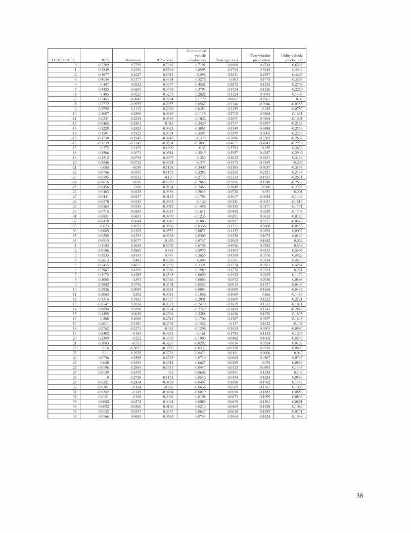
38

LEAD/LAGS WPI Aluminum IIP – basic

Commercial vehicle

production Passenger cars Two wheeler

production Utility vehicle

production

0 0.2209 0.2799 0.7061 0.7191 0.6008 0.4744 0.6343

-1 0.3249 0.2156 0.5549 0.6595 0.4793 0.3149 0.4949

-2 0.3677 0.1627 0.5311 0.596 0.3631 0.2397 0.4695

-3 0.4134 0.1177 0.4654 0.5276 0.303 0.1775 0.3363

-4 0.447 0.0522 0.3997 0.4521 0.2872 0.1225 0.2798

-5 0.4425 -0.0265 0.3768 0.3794 0.1724 0.1226 0.2263

-6 0.405 -0.0523 0.3233 0.2825 0.1124 0.0093 0.1403

-7 0.3465 -0.0842 0.2804 0.1779 0.0062 -0.0567 0.07

-8 0.2772 -0.0955 0.2055 0.0567 -0.1146 -0.2046 -0.0383

-9 0.1792 -0.1112 0.2069 -0.0454 -0.2139 -0.245 -0.0757

-10 0.1007 -0.1898 0.0689 -0.1115 -0.2715 -0.3568 -0.1631

-11 0.0231 -0.2234 0.0583 -0.1826 -0.2691 -0.3854 -0.1601

-12 -0.0465 -0.2501 -0.012 -0.2429 -0.3717 -0.4397 -0.2129

-13 -0.1229 -0.2423 -0.0425 -0.3051 -0.3349 -0.4488 -0.2156

-14 -0.1501 -0.1925 -0.0554 -0.3597 -0.3999 -0.5005 -0.2259

-15 -0.1758 -0.1942 -0.0643 -0.372 -0.3896 -0.5382 -0.2602

-16 -0.1739 -0.1345 -0.0594 -0.3807 -0.4677 -0.4843 -0.2938

-17 -0.172 -0.1429 -0.1009 -0.37 -0.3793 -0.459 -0.2624

-18 -0.1506 -0.1071 -0.0514 -0.3549 -0.3957 -0.4247 -0.2902

-19 -0.1312 -0.0758 -0.0979 -0.353 -0.3652 -0.4131 -0.3453

-20 -0.1246 -0.0722 -0.0924 -0.374 -0.3575 -0.3559 -0.296

-21 -0.085 -0.039 -0.1196 -0.3409 -0.3105 -0.3057 -0.3133

-22 -0.0746 -0.0355 -0.1172 -0.3283 -0.2355 -0.2521 -0.2494

-23 -0.0595 -0.0232 -0.127 -0.2775 -0.2333 -0.1931 -0.2651

-24 -0.0676 0.016 -0.1059 -0.2863 -0.2016 -0.1249 -0.2687

-25 -0.0456 0.06 -0.0624 -0.2463 -0.1849 -0.086 -0.2307

-26 -0.0403 0.0438 -0.0636 -0.2041 -0.0726 -0.031 -0.201

-27 -0.0441 0.0437 0.0123 -0.1783 -0.1017 0.0083 -0.1409

-28 -0.0578 0.0145 -0.0493 -0.142 0.0141 -0.0031 -0.1515

-29 -0.0563 0.0145 -0.0412 -0.1496 -0.0135 -0.0171 -0.1731

-30 -0.0715 0.0555 -0.0955 -0.1611 0.0482 -0.0229 -0.1704

-31 -0.0831 0.0601 -0.0899 -0.1235 0.0291 0.0053 -0.0785

-32 -0.0478 0.0644 -0.0945 -0.083 0.0987 0.0517 -0.0429

-33 -0.023 0.1023 -0.0586 -0.0336 0.1321 0.0608 -0.0159

-34 0.0065 0.1205 -0.0552 0.0071 0.1132 0.0934 0.0037

-35 0.0255 0.1331 -0.0368 0.0309 0.1338 0.1073 0.0166

-36 0.0915 0.1077 -0.029 0.0747 0.2063 0.1642 0.062

1 0.1183 0.3638 0.5799 0.6735 0.4996 0.3983 0.538

2 -0.0186 0.3869 0.585 0.5976 0.4403 0.4131 0.5603

3 -0.1533 0.4141 0.487 0.5655 0.4368 0.3376 0.4929

4 -0.2613 0.481 0.4338 0.494 0.3505 0.3614 0.4677

5 -0.3455 0.4657 0.3559 0.3321 0.2234 0.2861 0.4261

6 -0.3967 0.4709 0.3086 0.1989 0.1276 0.2763 0.221

7 -0.4172 0.4285 0.2545 0.0859 0.1922 0.2195 0.1479

8 -0.4005 0.391 0.1366 0.0053 0.0372 0.2036 0.0508

9 -0.3842 0.3796 0.0794 -0.0524 0.0015 0.1527 -0.0407

10 -0.2926 0.3009 0.0241 -0.0884 -0.0009 0.1668 -0.0492

11 -0.2063 0.292 -0.0011 -0.1802 -0.1069 0.166 -0.1458

12 -0.1314 0.1963 -0.1537 -0.2801 -0.1869 0.1222 -0.2121

13 -0.0547 0.1838 -0.0521 -0.2479 -0.1619 0.1513 -0.1871

14 0.0694 0.0208 -0.2264 -0.2749 -0.1418 0.1141 -0.2848

15 0.1495 -0.0638 -0.2206 -0.2288 -0.1626 0.1676 -0.1803

16 0.208 -0.1008 -0.2341 -0.1706 -0.1367 0.0997 -0.1648

17 0.2611 -0.1387 -0.2732 -0.1552 -0.117 0.1622 -0.105

18 0.2762 -0.1275 -0.352 -0.1298 -0.1053 0.0901 -0.0987

19 0.2402 -0.184 -0.3261 -0.161 -0.1795 0.1124 -0.1264

20 0.2309 -0.252 -0.3303 -0.1083 -0.0482 0.1002 -0.0243

21 0.2083 -0.332 -0.3227 -0.0292 -0.016 0.0324 0.0127

22 0.16 -0.3057 -0.3096 -0.0537 -0.0158 0.0516 0.0822

23 0.11 -0.2935 -0.3276 -0.0474 0.0101 0.0006 0.042

24 0.0736 -0.2398 -0.2725 -0.0719 -0.0063 -0.0367 0.0797

25 0.048 -0.3435 -0.3314 -0.0627 0.0289 -0.076 0.0559

26 -0.0196 -0.2983 -0.1933 -0.0447 0.0113 -0.0893 0.1143

27 -0.0139 -0.3319 -0.2 -0.0602 0.0591 -0.1228 0.109

28 0 -0.2738 -0.1152 -0.0542 0.0434 -0.1253 0.0539

29 -0.0321 -0.2434 -0.0458 -0.0407 0.1088 -0.1962 0.1143

30 -0.0301 -0.164 -0.086 -0.0634 0.0569 -0.1767 0.1005

31 -0.0202 -0.149 -0.0404 -0.0019 0.0818 -0.1883 0.0856

32 -0.0131 -0.108 0.0069 -0.0105 0.0673 -0.1999 0.0804

33 0.0052 -0.0372 0.0464 0.0083 0.0695 -0.1561 0.0891

34 0.0092 -0.0368 0.0166 0.0213 0.0463 -0.1838 0.1059

35 0.0132 0.0547 0.0967 0.0647 0.0618 -0.1859 0.0771

36 0.0166 0.0685 0.0585 0.0744 0.1064 -0.1624 0.1048

39

LEAD/LAGS India- exports IIP- Capital Aggr deposits

0 0.3295 0.68 0.0133

-1 0.3986 0.3728 0.0198

-2 0.5212 0.358 -0.047

-3 0.5289 0.4036 -0.033

-4 0.5276 0.3146 -0.0465

-5 0.5226 0.3103 -0.0575

-6 0.4893 0.3083 -0.0584

-7 0.4271 0.2293 -0.043

-8 0.3732 0.0225 -0.0391

-9 0.3443 -0.1323 -0.0629

-10 0.2943 -0.1067 -0.024

-11 0.2546 -0.1792 -0.0345

-12 0.2131 -0.2628 -0.012

-13 0.1871 -0.1761 -0.0096

-14 0.1977 -0.3346 0.034

-15 0.1647 -0.2457 0.0087

-16 0.1529 -0.2491 0.0491

-17 0.149 -0.1986 0.1219

-18 0.0649 -0.1717 0.1622

-19 0.0562 -0.168 0.196

-20 0.0132 -0.07 0.2572

-21 -0.0043 -0.1288 0.3122

-22 -0.0695 -0.0081 0.3222

-23 -0.0713 -0.1253 0.3667

-24 -0.1119 -0.0526 0.3843

-25 -0.1072 -0.0531 0.4131

-26 -0.1826 -0.0156 0.4398

-27 -0.1994 -0.0487 0.4635

-28 -0.1934 -0.0296 0.4561

-29 -0.2289 0.0043 0.4669

-30 -0.2115 -0.0292 0.4234

-31 -0.1845 0.0586 0.428

-32 -0.1681 0.0512 0.4148

-33 -0.2075 0.1283 0.3918

-34 -0.1283 0.0209 0.373

-35 -0.1357 0.113 0.3663

-36 -0.1096 0.0379 0.3482

1 0.3295 0.3111 0.0204

2 0.2892 0.2824 0.0136

3 0.1033 0.2099 0.0104

4 -0.0334 0.1954 -0.0042

5 -0.1099 0.1419 -0.003

6 -0.2193 0.1526 -0.0193

7 -0.3555 0.164 -0.0521

8 -0.411 -0.0757 -0.0145

9 -0.4848 -0.0804 -0.0739

10 -0.4874 -0.0607 -0.1018

11 -0.4955 -0.0629 -0.1365

12 -0.4296 -0.0947 -0.1443

13 -0.3817 -0.088 -0.175

14 -0.3076 -0.102 -0.1766

15 -0.2332 -0.1163 -0.1856

16 -0.1364 -0.1523 -0.2074

17 -0.0874 -0.0943 -0.1723

18 0.0179 -0.1004 -0.1763

19 0.0793 -0.0926 -0.1651

20 0.1691 -0.0758 -0.1511

21 0.1856 -0.0756 -0.1388

22 0.1978 -0.0673 -0.1237

23 0.2383 -0.0719 -0.0613

24 0.2064 -0.0433 -0.0862

25 0.1964 -0.0292 -0.0574

26 0.1706 -0.0175 -0.0491

27 0.1911 -0.0132 -0.0261

28 0.1577 -0.0081 -0.0322

29 0.0274 -0.0073 -0.0156

30 0.0518 -0.0006 0.01

31 0.0281 0.0131 -0.0635

32 -0.053 0.0097 -0.0341

33 -0.0275 -0.0026 -0.04

34 0.0207 -0.0216 -0.0244

35 -0.0853 -0.0059 -0.05

36 -0.0239 -0.0115 -0.0213