Embed Size (px)
Citation preview

Auralization of tonal rotor noise components of a quadcopter
flyover
Andrew Christiana
Structural Acoustics Branch, NASA Langley Research Center
Hampton, Virginia, 23681, USA
D. Douglas Boyd, Jr.,b Nikolas S. Zawodny,c and Stephen A. Rizzid
Aeroacoustics Branch, NASA Langley Research Center
Hampton, Virginia, 23681, USA
The capabilities offered by small unmanned vertical lift aerial vehicles, for example,
quadcopters, continue to captivate entrepreneurs across the private, public, and civil
sectors. As this industry rapidly expands, the public will be exposed to these devices (and to
the noise these devices generate) with increasing frequency and proximity. Accordingly, an
assessment of the human response to these machines will be needed shortly by decision
makers in many facets of this burgeoning industry, from hardware manufacturers all the
way to government regulators. One factor of this response is that of the annoyance to the
noise that is generated by these devices. This paper presents work currently being pursued
by NASA toward this goal. First, physics-based (CFD) predictions are performed on a
single isolated rotor typical of these devices. The result of these predictions are time
records of the discrete tonal components of the rotor noise. These time records are
calculated for a number of points that appear on a lattice of locations spread over the lower
hemisphere of the rotor. The source noise is then generated by interpolating between these
time records. The sound from four rotors are combined and simulated-propagation
techniques are used to produce complete flyover auralizations.
1 INTRODUCTION
With the continuing proliferation of small, unmanned, vertical-lift systems (sUAS) of all
sizes and flight capabilities, as well as the innumerable concepts that entrepreneurs around the
world have thought of for their use, it is likely only a matter of time before having swarms of
these machines in close proximity to humans becomes a problem. A likely arena of contention
will be the noise generated thereby. This study is a step on the path to being able to produce
a email: [email protected] b email: [email protected] c email: [email protected] d email: [email protected]
https://ntrs.nasa.gov/search.jsp?R=20160006429 2018-06-06T15:08:12+00:00Z
high-fidelity time-domain predictions of this sound based on simulations of sUAS that may or
may not yet exist. This capability will become critical to researchers attempting to understand the
factors that contribute to the human annoyance response generated by sUAS.
1.1 Operational Concepts
For smaller machines, like the quadcopter that is the focus of this study, the speeds of the
rotors (measured in revolutions-per-minute (RPM)) are controlled directly through variable-
speed motors. A simple proportional/integral/derivative (PID) closed-loop feedback control
system on the vehicle modulates these RPMs in order to maintain the vehicle’s attitude.
For instance, in the case of forward flight, the RPMs of the two stern motors are increased,
while the RPMs of the bow motors are kept near hover speed. This causes the vehicle to pitch
forward. The PID system maintains the overall lift of the machine in order to resist gravity, and
the component of the total force generated by the rotors that is not pointed directly skyward
causes a net thrust force to act on the vehicle generating motion in that direction. In reality, this
approach leads to constantly-changing rotor RPMs which in turn leads to perceptually significant
frequency variation of the rotor noise.
The vehicle used in this study is the DJI Phantom 2 pictured in Figure 1a. This vehicle was
among those included in a recent series of outdoor vehicle flight tests conducted by NASA. The
purpose of these flight tests was to acquire detailed acoustic and flight telemetry data for the
vehicle while operating under realistic flight conditions.
Some sample acoustic data from a forward-flight flyover run of the Phantom 2 is provided in
Figure 1b. The pairs of lines running relatively horizontally through the figure represent blade-
passage frequency (BPF) harmonics of the bow/stern pairs of rotors. (Note that there is a
constant offset within the pairs, perhaps generated by poor rotor manufacturing tolerance that is
compensated for by the PID controller.) Momentary variation within pairs indicates roll
compensation, and momentary variation between the pairs indicates pitch compensation. These
sorts of variations become clearly audible as the vehicle struggles to keep upright and aligned for
forward flight in the presence of wind, turbulence, and mass loading by the payload. These
variations are audible, and it is thought to be likely that the annoyance caused by sUAS will have
some component that is correlated with the attributes of these variations. The ability to
accurately auralize this noise would allow for the controlled human subject testing needed to
evaluate that (and other) factors that contribute to annoyance from these machines.
The remainder of this paper is divided into three main sections. First (Section 2), the effort
to produce a sufficiently accurate prediction of the sound generated by a single isolated rotor is
detailed. Then, in Section 3, a method of turning this prediction into a time-history at a receiver
given some simulated flight path are developed. In Section 4 two example complete flyover
events are produced and discussed.
2 SOURCE NOISE PREDICTION
2.1 On the Subject of ‘Tonality’
First, an important technical concept behind all of the steps in this study is that a Discrete
Fourier Transform (DFT) of a time record of length 𝐿 (measured in seconds) will only contain
frequencies that are harmonics of 1/𝐿 (a frequency measured in Hertz).1 This implies that a
record of a single blade passage will only contain information at the blade passage harmonics.
During the auralization process, these harmonic components will be summed as a discrete series

of cosines so that this process will output only ‘tonal’ source noise. Therefore, if there is noise or
unsteadiness present in the method used to produce the input single blade passage record (e.g.
deterministic non-periodicity in a computational fluid dynamics (CFD) simulation), the
auralization process will ascribe that unsteady energy into the tonal component in the output.
Not included in this study will be broadband noise that is generated by these vehicles (e.g.
rotor blade trailing edge noise). Also, although it is harmonically related to the BPF, noise
generated by the electric motors that drive the rotors is also not included.
(a)
(b)
Figure 1 – (a) Photograph of the DJI Phantom 2 quadcopter in hover. (b) Example acoustic
spectrogram from a forward-flight flyover event in an outdoor environment.
2.2 Why Compute?
It is highly advantageous to use a computational method to generate the source data for a
time-domain auralization effort such as this. For the auralization processes detailed in Section 3,
a good deal of data is needed spread over a lower-hemisphere in the acoustic far-field of the
rotor. The cost in time and/or equipment is prohibitive to acquire this data experimentally.
Therefore, in this study, a CFD prediction is generated (Section 2.4), and then compared to
recordings of a real-world test using a similar configuration at a subset of locations (Sections 2.5
and 2.6). When these two compare well, the prediction is then used with some confidence to
generate the data required for auralization. In particular, the configuration that is studied in this
section is a single isolated rotor. The flight condition is that of a nominal hover condition.
2.3 Vehicle Description
The sUAS platform focused on in this study is the DJI Phantom 2 quadcopter, as mentioned
earlier and shown in Figure 1a. This vehicle is a representative small-scale machine that is
affordable to the typical consumer. The vehicle consists of four rotors, each of which has two
blades and is powered by a three-phase brushless electric motor. Two different sets of rotor
blades were considered: those provided by the manufacturer (DJI), and a second set of blades
made of carbon fiber (CF) manufactured by a third party. Ideally, these two sets of blades would
share the exact same geometry. For instance, they share the same rotor diameter 𝑅 =12.1 𝑐𝑚 (4.75 𝑖𝑛). At the onset of testing it was observed that the DJI rotors exhibited much
more uniformity in blade surface features and blade shape as compared to the CF blades. In
addition, the CF blades were much more rigid than the DJI blades.
2.4 Single-rotor CFD Run
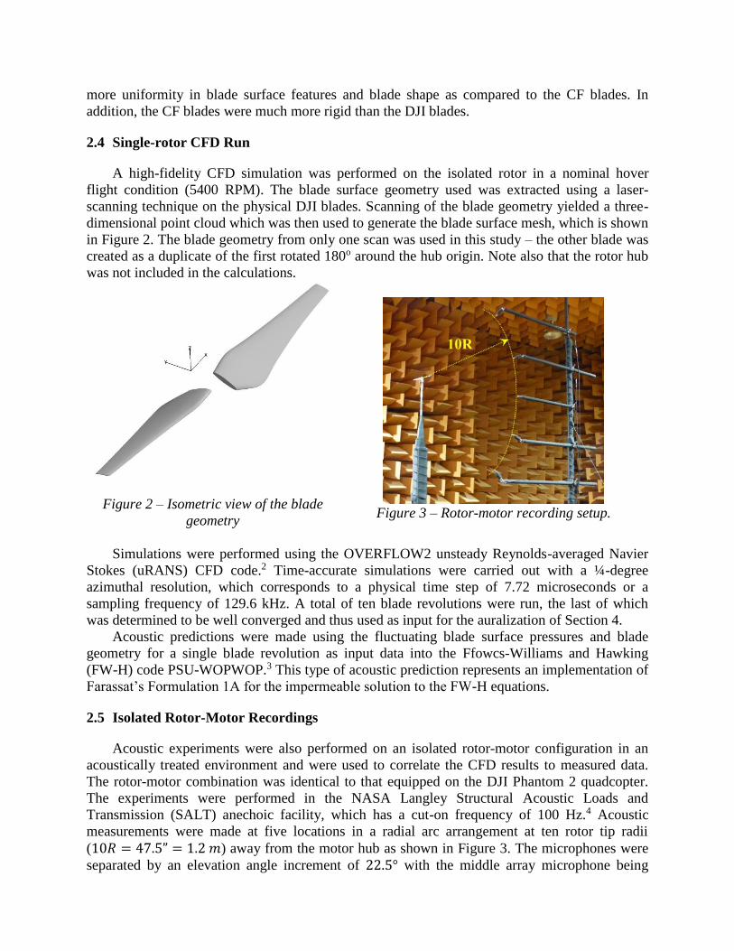
A high-fidelity CFD simulation was performed on the isolated rotor in a nominal hover
flight condition (5400 RPM). The blade surface geometry used was extracted using a laser-
scanning technique on the physical DJI blades. Scanning of the blade geometry yielded a three-
dimensional point cloud which was then used to generate the blade surface mesh, which is shown
in Figure 2. The blade geometry from only one scan was used in this study – the other blade was
created as a duplicate of the first rotated 180o around the hub origin. Note also that the rotor hub
was not included in the calculations.
Figure 2 – Isometric view of the blade
geometry
Figure 3 – Rotor-motor recording setup.
Simulations were performed using the OVERFLOW2 unsteady Reynolds-averaged Navier
Stokes (uRANS) CFD code.2 Time-accurate simulations were carried out with a ¼-degree
azimuthal resolution, which corresponds to a physical time step of 7.72 microseconds or a
sampling frequency of 129.6 kHz. A total of ten blade revolutions were run, the last of which
was determined to be well converged and thus used as input for the auralization of Section 4.
Acoustic predictions were made using the fluctuating blade surface pressures and blade
geometry for a single blade revolution as input data into the Ffowcs-Williams and Hawking
(FW-H) code PSU-WOPWOP.3 This type of acoustic prediction represents an implementation of
Farassat’s Formulation 1A for the impermeable solution to the FW-H equations.
2.5 Isolated Rotor-Motor Recordings
Acoustic experiments were also performed on an isolated rotor-motor configuration in an
acoustically treated environment and were used to correlate the CFD results to measured data.
The rotor-motor combination was identical to that equipped on the DJI Phantom 2 quadcopter.
The experiments were performed in the NASA Langley Structural Acoustic Loads and
Transmission (SALT) anechoic facility, which has a cut-on frequency of 100 Hz.4 Acoustic
measurements were made at five locations in a radial arc arrangement at ten rotor tip radii
(10𝑅 = 47.5” = 1.2 𝑚) away from the motor hub as shown in Figure 3. The microphones were
separated by an elevation angle increment of 22.5° with the middle array microphone being

located on the rotor tip-path plane (elevation angle 𝜃 = 0°). This radial distance was selected
because it was the minimum distance where the overall integrated acoustic sound pressure levels
of the rotor-motor pair exhibited spherical spreading (i.e. the microphones were placed at the
beginning of the acoustic far field). The microphones used were G.R.A.S. Type 40AQ ½”
diameter pre-polarized random incidence microphones. The rotor blades were located
approximately 15𝑅 above the floor wedge tips in order to minimize flow-recirculation effects.
2.6 Data Acquisition and Processing
Microphone acoustic pressure time histories were acquired at a sampling rate of 20 kHz for
a duration of 10 seconds. As the BPF of the test case is 180 Hz, a 10 Hz binwidth DFT was
desired in order to produce an on-bin condition for the BPF harmonics while providing sufficient
bin density to resolve the broadband component. This implies dividing each recording up into
100 blocks of 2,000 samples each. The resulting Hanning-windowed power-spectral density
functions (PSD) were averaged across the blocks to produce a single PSD for each recording. 5
In order to make direct comparisons with the acoustic predictions discussed in Section 2.4,
some additional processing of the experimental data was required. In order to account for the
combined effects of slight variations in rotor rotation rate and spectral leakage, a scheme for
separating the raw experimental acoustic spectrum into its broadband and tonal components is
implemented. This method is adapted from that detailed in Reference 6. A sample experimental
spectrum that has undergone this processing is shown in Figure 4.
Figure 4 – Example of post-processed experimental data. (Note: data shown is for the DJI
rotor blades at an elevation angle of 𝜃 = −22.5∘)
2.7 Comparison of Tonal Components
A comparison between the predictions and experimental data of the BPF sound pressure
level (SPL) is shown in Figure 5a. As these results show, good agreement is obtained between
the BPF level predictions and experimental DJI blade measurements for all measured observer
angles. Comparison with the CF blades yields less favorable results overall, however they exhibit
the same good agreement at higher elevation angles.
Figure 5b presents a tonal spectral comparison between prediction and experiments at an
elevation angle of 𝜃 = −22.5∘. It is important to note that the experimental data are
contaminated with noise from the electric motor over a subset of the frequency range of interest.
This is indicated in the figure as a shaded region. The data shown in Figure 5b display mixed

results, with the 1st and 2nd BPF harmonics of both blade sets comparing favorably with the
prediction, then showing considerable disagreement at the 3rd and 4th harmonics. Observation of
the 8th – 20th harmonics shows better agreement between the CF blade experiment and prediction
results as compared to those of the DJI blades. The exact cause of this is not known, however is
believed to be related to the loading conditions of the rigid CF blades more accurately
representing those of the blades in the (perfectly rigid) CFD prediction.
Given the agreement between the CFD prediction and the measurements, a dataset created
from the prediction is deemed to be suitable as the basis for the auralization effort. The
remainder of this effort is focused on the creation of an auralization scheme for this class of
noise. Therefore a basis dataset can be ‘suitable’ as long as it is close enough to be representative
of this type of rotor noise, even if there are disparities that may be audible.
(a)
(b)
Figure 5 – Comparisons between recording and CFD prediction: (a) SPL of BPF versus
elevation angle, (b) SPL of BPF harmonics versus frequency for θ = -22.5° (the
shaded region represents motor noise contamination, BPF = 180 Hz).
3 AURALIZATION TECHNIQUE
This section describes the process by which the information contained in the CFD prediction
is transformed into an auralization of a complete flyover event. First, the data has to be cast into
a usable (hemisphere) form. Then, Sections 3.2 – 3.4 detail the process by which a single point in
a time record of a single rotor source is created. This includes using two steps of interpolation to
produce a spectrum of the tonal noise at a given emission angle, and then an additive synthesis
method to bring that information into the time domain. (Ideally, these steps would be followed
for each sample in the output source noise time record, as the angle desired is changing for each
sample.) This source noise is then propagated to a virtual receiver location.
3.1 Technical Description of the Source Hemisphere
The form of the CFD data that will be useful for the auralization process is that of a
rectangular lattice over a hemisphere underneath the rotor. Consider a sphere, the radius of which
is the minimum far field acoustic distance from the rotor (determined to be 1.2 𝑚 in Section 2.5).
The hemisphere that is used is this sphere bisected by the tip-path plane, keeping only the half
closer to the ground (under normal hover conditions).
The specific formalism for the geometry of the lattice comes from that used by the ANOPP
program.7 This is a spherical coordinate system whereby the ‘north pole’ at 0-elevation (𝜃 = 0°)
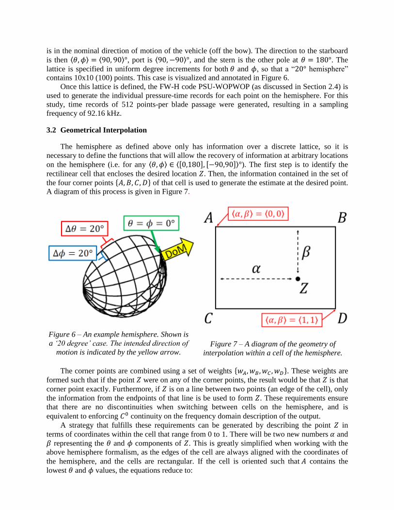
is in the nominal direction of motion of the vehicle (off the bow). The direction to the starboard
is then ⟨𝜃, 𝜙⟩ = ⟨90, 90⟩°, port is ⟨90, −90⟩°, and the stern is the other pole at 𝜃 = 180°. The
lattice is specified in uniform degree increments for both 𝜃 and 𝜙, so that a “20° hemisphere”
contains 10x10 (100) points. This case is visualized and annotated in Figure 6.
Once this lattice is defined, the FW-H code PSU-WOPWOP (as discussed in Section 2.4) is
used to generate the individual pressure-time records for each point on the hemisphere. For this
study, time records of 512 points-per blade passage were generated, resulting in a sampling
frequency of 92.16 kHz.
3.2 Geometrical Interpolation
The hemisphere as defined above only has information over a discrete lattice, so it is
necessary to define the functions that will allow the recovery of information at arbitrary locations
on the hemisphere (i.e. for any ⟨𝜃, 𝜙⟩ ∈ ⟨[0,180], [−90,90]⟩°). The first step is to identify the
rectilinear cell that encloses the desired location 𝑍. Then, the information contained in the set of
the four corner points {𝐴, 𝐵, 𝐶, 𝐷} of that cell is used to generate the estimate at the desired point.
A diagram of this process is given in Figure 7.
Figure 6 – An example hemisphere. Shown is
a ‘20 degree’ case. The intended direction of
motion is indicated by the yellow arrow.
Figure 7 – A diagram of the geometry of
interpolation within a cell of the hemisphere.
The corner points are combined using a set of weights {𝑤𝐴, 𝑤𝐵, 𝑤𝐶 , 𝑤𝐷}. These weights are
formed such that if the point 𝑍 were on any of the corner points, the result would be that 𝑍 is that
corner point exactly. Furthermore, if 𝑍 is on a line between two points (an edge of the cell), only
the information from the endpoints of that line is be used to form 𝑍. These requirements ensure
that there are no discontinuities when switching between cells on the hemisphere, and is
equivalent to enforcing 𝐶0 continuity on the frequency domain description of the output.
A strategy that fulfills these requirements can be generated by describing the point 𝑍 in
terms of coordinates within the cell that range from 0 to 1. There will be two new numbers 𝛼 and
𝛽 representing the 𝜃 and 𝜙 components of 𝑍. This is greatly simplified when working with the
above hemisphere formalism, as the edges of the cell are always aligned with the coordinates of
the hemisphere, and the cells are rectangular. If the cell is oriented such that 𝐴 contains the
lowest 𝜃 and 𝜙 values, the equations reduce to:

𝛼 =𝑍𝜃 − 𝐵𝜃𝐴𝜃 − 𝐵𝜃
𝑎𝑛𝑑 𝛽 =𝑍𝜙 − 𝐶𝜙
𝐴𝜙 − 𝐶𝜙 →
{
𝑤𝐴 = (1 − 𝛼) ∙ (1 − 𝛽)
𝑤𝐵 = (1 − 𝛼) ∙ 𝛽
𝑤𝐶 = 𝛼 ∙ (1 − 𝛽)
𝑤𝐷 = 𝛼 ∙ 𝛽
(1)
3.3 Frequency-domain Interpolation
Once the set of weights has been calculated for the desired emission angle they can be used
in a weighted average over both the magnitude 𝑀𝑛,𝑖 and phase 𝜑𝑛,𝑖 of the cell corner points,
respectively:
𝑀𝑛,𝑍 =∑[𝑤𝑖 ∙ 𝑀𝑛,𝑖]
∑𝑤𝑖 𝑎𝑛𝑑 𝜑𝑛,𝑍 =
∑[𝑤𝑖 ∙ 𝜑𝑛,𝑖]
∑𝑤𝑖 𝑤ℎ𝑒𝑟𝑒 {
𝑛 = 1…𝑁 𝑖 = {𝐴, 𝐵, 𝐶, 𝐷}
(2)
Here 𝑁 is the total number of BPF harmonics contained in the input data set, and 𝑀𝑛,𝑍 and 𝜑𝑛,𝑍
are the magnitude and phase at the point Z, respectively. Although there are several drawbacks to
using this scheme, especially on the phase information, it has several advantageous properties.
This method is very fast, and can be computed over vectors (instead of for individual harmonics)
without the use of conditional statements.
3.4 Additive Synthesis
Once the frequency-domain information at the point 𝑍 has been interpolated, the acoustic
pressure time history at the source can be generated via an additive synthesis technique:
𝑝(𝑡) = ∑(𝑀𝑛 +𝑀�̃�(𝑡)) ∙ 𝑐𝑜𝑠(2𝜋 ∙ 𝑛 ∙ ℛ(𝑡) + 𝜑𝑛 + 𝜑�̃�(𝑡))
𝑁
𝑛=1
(3)
As 𝑛 = 0 represents the DC component of the DFT, beginning at 𝑛 = 1 removes any DC from
the prediction. Here 𝑁 is selected such that the highest harmonic included in the summation does
not exceed the Nyquist frequency of the source noise time record (in order to avoiding aliasing).
The ‘tilde’ terms are possible time-varying elements of the magnitude and phase of the rotor due
not to broadband noise, but perhaps to periodically changing loading conditions. These functions
would be expected to vary slowly over the period of multiple blade passages. Modulating
components of this type have been shown to be perceptually significant for full-scale rotorcraft.8
The function ℛ(𝑡) in Eqn. 3 represents the instantaneous rotor azimuthal angle. In practice,
it is a number that is varying between 0 and 1, and is updated at every time step given the current
BPF and previous rotor state:
ℛ(𝑡 + Δ𝑡) = mod(𝑅(𝑡) + 𝐵𝑃𝐹(𝑡) ∙ Δ𝑡, 1) (4)
This generalizes the concept of the RPM of the vehicle that is being simulated and allows,
for instance, for RPM to vary with time as was seen in Fig. 1b.
3.5 Interpolation Analysis
At this point, it is important to verify the operation of the interpolation process described
above. When working correctly, the scheme should be operating within a ‘scaling region.’9 In
this region, the error produced at the output is related to the distance over which one is
interpolating raised to some power. This could be written as 𝜀 ∝ ℎ𝑝 where 𝜀 is a measure of the
error, ℎ is the distance over which the interpolator is working, and 𝑝 is the scaling power of the
interpolation scheme. If ℎ is too large the output may be completely incorrect – just a naïve mash
of the input data. If ℎ is too small the interpolation scheme becomes susceptible to numerical
errors. Therefore, the goal is to determine a parsimonious ℎ such that the interpolator is
producing results that are reasonable while not requiring unnecessarily high data-density.
For this verification, the error 𝜀 is taken as the RMS value of the residual signal that is
generated when the interpolator is asked to estimate a full blade passage time series at a known
point. The distance ℎ is the mean great circle distance between the four points used in the
estimation and the estimated point. Computing over a large number of known points, it is found
that the upper-bound for the scaling region for this interpolation problem occurs at
approximately a hemisphere step size of 15°. The lower bound is limited by the memory
requirements of the scheme. It is important to note that this result is not extensible, and that even
different data conditions (e.g. non-hover prediction cases) could lead to a different data-density
requirement.
3.6 A Set of Four Rotors
To generate the source noise from a quadcopter, four of these individual rotor records need
to be made – one for each rotor. These will have to be calculated independently for two reasons:
1. Half of the rotors will have their geometry reversed in order to simulate the correct
clockwise/anti-clockwise pairing scheme.
2. There will be small differences in the desired emission angle between the four rotors
because they are physically separated from each other by the size of the vehicle (see
Fig. 1a). This separation is important to maintain as it is a requisite for correct
prediction of the far-field total radiation/interference pattern of the vehicle.
3.7 Simulated Propagation Processing
Once the four independent tonal rotor source noise records have been generated, they are
propagated to a virtual receiver point. Briefly, this processing takes the form of several layers of
digital signal processing that emulate:
1. A dynamic time delay element resulting in a Doppler shift for moving sources.
2. A gain term to account for spherical spreading losses over distance.
3. A range-dependent FIR filter to account for atmospheric absorption losses.
4. A propagation path to represent the sound that is reflected by the ground surface to
the receiver location creating interference effects with the direct path.
Further details of these various steps are available in other publications. 10, 11
4 AN EXAMPLE AURALIZED FLYOVER
This section presents the development of two complete auralized flyover events. These
auralizations use nominal quantities from the flyover recording that produced the spectrogram of
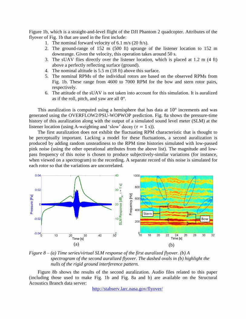
Figure 1b, which is a straight-and-level flight of the DJI Phantom 2 quadcopter. Attributes of the
flyover of Fig. 1b that are used in the first include:
1. The nominal forward velocity of 6.1 m/s (20 ft/s).
2. The ground-range of 152 m (500 ft) uprange of the listener location to 152 m
downrange. Given the velocity, this operation takes around 50 s.
3. The sUAV flies directly over the listener location, which is placed at 1.2 m (4 ft)
above a perfectly reflecting surface (ground).
4. The nominal altitude is 5.5 m (18 ft) above this surface.
5. The nominal RPMs of the individual rotors are based on the observed RPMs from
Fig. 1b. These range from 4600 to 7000 RPM for the bow and stern rotor pairs,
respectively.
6. The attitude of the sUAV is not taken into account for this simulation. It is auralized
as if the roll, pitch, and yaw are all 0°.
This auralization is computed using a hemisphere that has data at 10° increments and was
generated using the OVERFLOW2/PSU-WOPWOP prediction. Fig. 8a shows the pressure-time
history of this auralization along with the output of a simulated sound level meter (SLM) at the
listener location (using A-weighting and ‘slow’ decay (𝜏 = 1 s)).
The first auralization does not exhibit the fluctuating RPM characteristic that is thought to
be perceptually important. Lacking a model for these fluctuations, a second auralization is
produced by adding random unsteadiness to the RPM time histories simulated with low-passed
pink noise (using the other operational attributes from the above list). The magnitude and low-
pass frequency of this noise is chosen to produce subjectively-similar variations (for instance,
when viewed on a spectrogram) to the recording. A separate record of this noise is simulated for
each rotor so that the variations are uncorrelated.
(a)
(b)
Figure 8 – (a) Time series/virtual SLM response of the first auralized flyover. (b) A
spectrogram of the second auralized flyover. The dashed ovals in (b) highlight the
nulls of the rigid ground interference pattern.
Figure 8b shows the results of the second auralization. Audio files related to this paper
(including those used to make Fig. 1b and Fig. 8a and b) are available on the Structural
Acoustics Branch data server:
http://stabserv.larc.nasa.gov/flyover/

Inspecting Figures 1b and 8b and listening to the recordings on which they are based, the
major perceptual differences between the auralization and the recording appear to be:
1. The lack of sound power below the BPF in the auralization. This is primarily due to
wind and ambient noise in the recording.
2. The lack of broadband noise generated by the rotors. This is especially apparent
when the vehicle is in the ‘overhead’ position (⟨𝜃, 𝜙⟩ = ⟨90, 0⟩°, near 24 s).
3. A variation in the balance of sound power between higher BPF harmonics for the
stern rotors. This could be due to any number of things: the variation of the RPM
between the bow and stern rotors, a change in inflow condition for forward-flight,
etc. This may also be due to the absence of electric motor tones (as in Fig. 5b).
4. The lack of synchronization of the RPM-modulation of the rotors.
5. The use of a rigid ground model. This makes the ground interference pattern very
noticeable in Fig. 8b, whereas it is perhaps completely absent (and masked by
ambient noise) in Fig. 1b.
Many other differences, subjective and objective, are likely to exist between the two time
series in this initial effort. Of the above, differences 2 – 5 are issues that need to be addressed.
Solutions to differences 2 and 5 can likely be based on practices that are currently in use in other
auralization efforts.12
5 CONCLUSION
In this paper, the problem of auralizing the noise generated by a particular sUAS was
discussed. A physics-based (CFD) noise prediction was generated based on the geometry and
operating condition of a currently available quadcopter rotor. This prediction was shown to
compare well with recordings made of the isolated motor/rotor configuration. A method was
proposed to turn this prediction into an auralization, and the accuracy of that method was
verified. The resulting auralization compared reasonably well with a recording of a sUAS flyover
given the limitations and omissions of the current auralization process.
In the future, work to improve this overall process will proceed along several fronts:
1. The addition of other sources of noise from the vehicle such as broadband rotor noise
and motor noise.
2. The addition of further objective sources of RPM variation. These could come in the
form of simulated flight-dynamics models, or from empirical data as in Reference 8.
3. Rotor inflow effects including the interaction of one rotor with another.
4. Improvement or abandonment of the current hemisphere/interpolation paradigm.
Further, with this work as a basis, engineering predictions can begin to be made for use in
human subject tests to determine the annoyance caused by sUAVs, with the ultimate goal of
using these predictions to achieve perception-influenced low-noise design.
6 ACKNOWLEDGEMENTS
This research was supported by the National Aeronautics and Space Administration,
Aeronautics Research Mission Directorate, Transformative Aeronautics Concepts Program,
Convergent Aeronautics Solutions Project, Vertical Lift Hybrid Autonomy subproject.
Thanks to Ferdinand Grosveld of the Northrop Grumman Corporation for his work in
organizing the sUAV flyover tests, the data of which appears in Figure 1b and was used to
determine parameters for the auralizations.
7 REFERENCES
1. A. V. Oppenheim and R. W. Schafer, “Discrete-time Signal Processing (3rd Ed.),” Prentice
Hall, Upper Saddle River, NJ (2010).
2. P. G. Buning, R. J. Gomez, and W. I. Scallion, “CFD Approaches for Simulation of Wing-
Body Stage Separation,” in 22nd Applied Aerodynamics Conference and Exhibit, AIAA Paper
2004-4838, Providence, RI (2004)
3. K. S. Brentner and F. Farassat, “Modeling aerodynamically generated sound of helicopter
rotors,” Prog. Aerosp. Sci., 39, pp. 83-120, (2003)
4. F. W. Grosveld, “Calibration of the Structural Acoustics Loads and Transmission Facility at
NASA Langley Research Center,” InterNoise 1999, Fort Lauderdale, FL, 1999.
5. J. S. Bendat and A. G. Piersol, “Random Data (4th Ed.),” John Wiley & Sons, Hoboken, NJ
(2010).
6. S. A. Rizzi, D. B. Stephens, J. J. Berton, D. E. Van Zante, J. P. Wojno, and T. W. Goerig,
“Auralization of Flyover Noise from Open Rotor Engines Using Model Scale Test Data,” in
20th AIAA/CEAS Aeroacoustics Conference, AIAA Paper 2014-2750, Atlanta, GA (2014)
7. W. E. Zorumski “Aircraft noise prediction program theoretical manual,” NASA Technical
Report, NASA-TM-83199 PT-1 and PT-2 (1982).
8. J. R. Hardwick, A. Christian, and S. A. Rizzi, “Evaluation of the Perceptual Fidelity of a
Novel Rotorcraft Noise Synthesis Technique,” The Journal of the Acoustical Society of
America, 136, 2287-2287 (2014).
9. K. Atkinson and W. Han, “Elementary Numerical Analysis (3rd Ed.),” John Wiley & Sons,
Hoboken, NJ (2004).
10. S. A. Rizzi and B. M. Sullivan, “Synthesis of Virtual Environments for Aircraft Community
Noise Impact Studies,” Proceedings of the 11th AIAA/CEAS Aeroacoustics Conference,
AIAA-2005-2983, Monterey, CA, USA, 23-25 May 2005.
11. S. A. Rizzi, B. M. Sullivan, and Aric R. Aumann, "Recent developments in aircraft flyover
noise simulation at NASA Langley Research Center," NATO Research and Technology
Agency AVT-158 "Environmental Noise Issues Associated with Gas Turbine Powered
Military Vehicles" Specialists' Meeting, NATO RTA Applied Vehicle Technology Panel,
Paper 17, Montreal, Canada, (2008).
12. S. A. Rizzi and A. Christian “A method for simulation of rotocraft fly-in noise for human
response studies,” InterNoise 2015, San Francisco, CA, 2015.