august 2010 working paper - Mercatus Center

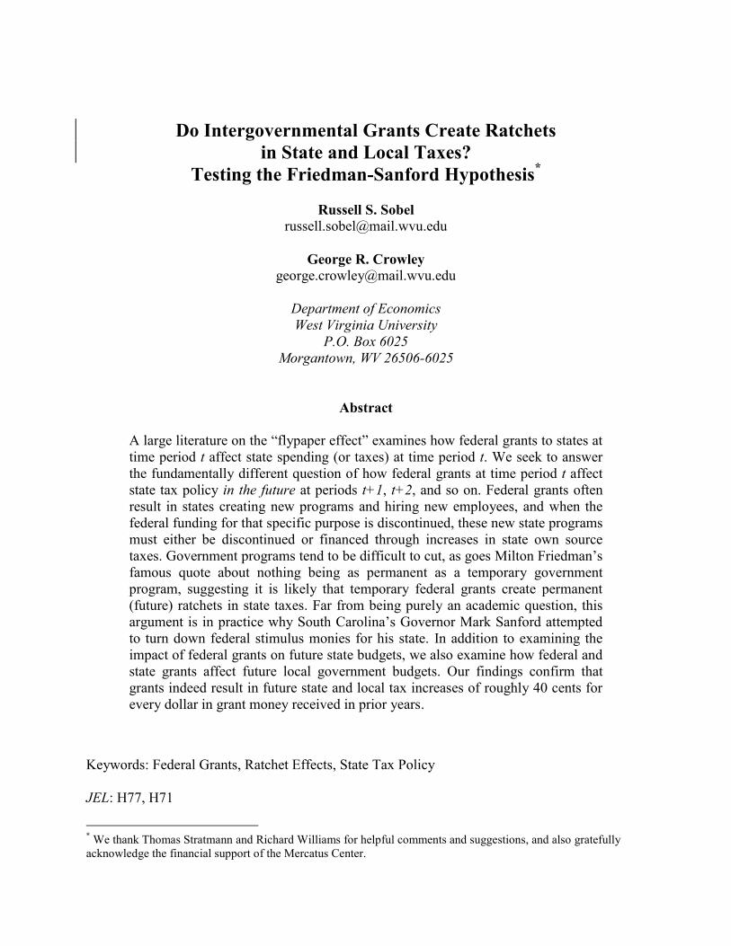
working paperDo intergovernmental grants create ratchets in state anD local taxes? testing the Friedman-sanford hypothesis

By Russell S. Sobel and George R. Crowley

no. 10-51 august 2010

The ideas presented in this research are the authors’ and do not represent official positions of the Mercatus Center at George Mason University.

Do Intergovernmental Grants Create Ratchets

in State and Local Taxes?

Testing the Friedman-Sanford Hypothesis*

Russell S. Sobel

[email protected]

George R. Crowley

[email protected]

Department of Economics

West Virginia University

P.O. Box 6025

Morgantown, WV 26506-6025

Abstract

A large literature on the ―flypaper effect‖ examines how federal grants to states at

time period t affect state spending (or taxes) at time period t. We seek to answer

the fundamentally different question of how federal grants at time period t affect

state tax policy in the future at periods t+1, t+2, and so on. Federal grants often

result in states creating new programs and hiring new employees, and when the

federal funding for that specific purpose is discontinued, these new state programs

must either be discontinued or financed through increases in state own source

taxes. Government programs tend to be difficult to cut, as goes Milton Friedman‘s

famous quote about nothing being as permanent as a temporary government

program, suggesting it is likely that temporary federal grants create permanent

(future) ratchets in state taxes. Far from being purely an academic question, this

argument is in practice why South Carolina‘s Governor Mark Sanford attempted

to turn down federal stimulus monies for his state. In addition to examining the

impact of federal grants on future state budgets, we also examine how federal and

state grants affect future local government budgets. Our findings confirm that

grants indeed result in future state and local tax increases of roughly 40 cents for

every dollar in grant money received in prior years.

Keywords: Federal Grants, Ratchet Effects, State Tax Policy

JEL: H77, H71

* We thank Thomas Stratmann and Richard Williams for helpful comments and suggestions, and also gratefully

acknowledge the financial support of the Mercatus Center.

2

Do Intergovernmental Grants Create Ratchets in State and Local

Taxes? Testing the Friedman-Sanford Hypothesis

“Nothing is so permanent as a temporary government program.”

—Nobel Laureate Milton Friedman (The Yale Book of Quotations, 2006)1

I. Introduction

As the opening quote from Nobel Laureate Milton Friedman illustrates, government programs

can be hard to discontinue once they are created. The many New Deal programs still in

existence seem to fit into this category.2 In his book, Crisis and Leviathan, Higgs (1987) even

proposes a ratchet theory of government growth in which temporary government programs that

are enacted in response to major crisis events become permanent, thereby providing an

explanation for historical government growth.3 Most recently, the federal stimulus response to

the financial crisis has brought about a large increase in federal government spending

accompanied by a host of new government programs that may linger much longer than

anticipated.

A significant amount of the recent expansion in government spending has been carried

out through a major increase in federal grants to states and local governments for new ―shovel-

ready‖ projects. If these temporary programs are hard to eliminate in the future, their

permanence will require states and localities to eventually raise their own taxes to fund these

programs once the federal funds are gone. Far from always being an unintended consequence,

some federal grants are made with the intention that states will pick up funding the program in

the future. In 2010, for example, the city of Morgantown, West Virginia, along with 39 other

cities, began receiving federal funding for the hiring of two new police officers for three years,

3

after which time the city will have to fund these new permanent full-time positions using own

source revenue.

The general question of whether federal grants to states cause subsequent state (or local)

tax increases is the topic we explore in this paper. The implications are important because if this

is the case, then the recent federal fiscal stimulus should not only be predicted to cause a

permanent ratchet upward in federal spending, but also a permanent ratchet in the size of state

and local governments in the United States. Far from being purely an academic question, this

argument is in practice why South Carolina‘s Governor Mark Sanford attempted to turn down

part of the federal stimulus monies for his state. Referring to when the temporary federal

stimulus funding runs out two years in the future, he states:

―Who helps us then? Do we raise taxes … or do we just summarily end

programs … [o]r are we to plan on yet another round of stimulus windfall

from Washington in two years … The easiest of all things would be to take

and simply spend all of Washington‘s well-intended stimulus efforts—but

in our case it would guarantee opportunities lost that I don‘t think our state

can afford.‖

South Carolina Governor Mark Sanford ―Prudence on Stimulus in State‘s

Best Interest,‖ Myrtle Beach Sun-News, April 6, 2009.

There is a rather large literature examining how federal grants at time period t affect state

or local spending (or taxes) during the same time period t (i.e., the ―flypaper effect‖ literature).

That literature asks whether federal grants tend to truly expand state spending (that is, ―stick‖),

or whether recipients instead use some of the funding to offset current taxes or to fund other

programs through reallocations of fungible resources in the period of the grant. We discuss this

literature in our paper because it will be important to account for it in our empirical analysis,

however, what we seek to answer in this paper is a fundamentally different question unaddressed

in the current literature: How do current federal grants at time t affect state and local tax policy in

4

the future? Our analysis attempts to answer this question using data on state revenue measures

and federal grants, as well as a sample of local governments in Pennsylvania. Our results do

indeed confirm the hypothesis that federal grants result in future increases in state and local taxes

and own source revenue.

We will proceed as follows. Section II will discuss the reasons why temporary

government programs tend to have permanence. Section III will review the literature on the

―flypaper effect‖ because our estimation will require that we control for this in the estimation.

Section IV discusses our data and presents our empirical results. Section V examines whether

grants from different federal agencies tend to differ in their impact on future taxes. Section VI

examines the impact of federal grants on individual tax rates and revenue sources for state

governments, section VII explores the impact of federal and state grants on local own source

revenue, and section VIII concludes.

II. Nothing is so Permanent as a Temporary Government Program

While one can find quotes from several notable individuals, such as the paper‘s opening quote by

Milton Friedman, that state the observation that temporary programs tend to become permanent,

it is worthwhile to briefly address the reasons why this may occur from the academic literature.

First, spending programs create their own new political constituency, in that the

government employees and private recipients whose incomes depend on the program, and their

families, will use political pressure to fight against any discontinuation of the program [see

Musgrave (1981) and Cullis and Jones (1998), chapter 14]. Regardless of the overall necessity

or efficiency of the program, there are always individuals who benefit from government

spending, and in fact these pecuniary gains to factor owners are often the primary justification

5

for legislative support for particular government projects [see Weingast, Shepsle, and Johnsen

(1981)].

Secondly, recent work in development economics shows that the resource windfalls to

different governments generated by foreign aid (which, in a sense, is what the federal

government is to state governments) intensify political struggles over control of the new

government resources [see Djankov, Montalvo, and Reynal-Querol (2008)]. A similar

phenomenon has been found to happen when states receive massive inflows of FEMA assistance

after a disaster [see Leeson and Sobel (2008)]. With more government funds comes additional

fights over political resource allocations, and an expansion in the rent-seeking industry occurs.4

The new resources that flow into lobbying then gain experience through time at how do so

effectively and become permanently more productive at producing political pressure [see Becker

(1983)].5 This lobbying-industry specific human and physical capital, if and when the external

aid disappears, then shifts focus toward gaining additional control over internal domestic

government spending. In a similar manner, federal grants may result in an expansion in state

lobbying activity that is successful in gaining influence over future state spending.

Third, Higgs (1987, p. 73) discusses reasons why increases (―ratchets‖) in government

spending do not entirely fade through time. He points to ideological change and ―the politics of

entrenched bureaucrats, their clients, and connected politicians.‖ In this manner, even the clients

and politicians who fund these programs become a force arguing for the continuation of

temporary programs.

It is important to be clear that in some cases the future state financing of the program is

not an unintended consequence, but is rather part of the explicit design of the federal grant. The

6

federal grants mentioned earlier in the introduction that helped cities hire new police officers for

three years were designed with the intention of requiring future local financing in the future.

In addition, different government grants are indeed different, and some may be more

likely to result in the creation of permanent programs than others. Funds to repave an existing

highway, for example, do not as obviously require a commitment of future resources, and even if

the funding was to build a new road, the permanent future costs would only be on the

maintenance of the road (a much smaller amount than the cost of grant funded construction).

Thus, the expectation for our empirical testing is that we should see the impact of $1 in

government grants creating somewhat less than $1 in future tax increases as only part of the

spending may become permanent. Because it is impossible to break out data on federal grants

into which funding is temporary versus permanent, we simply note that our data uses all federal

grants and that therefore we need to interpret the results with this in mind.

More importantly, if the federal grant does not expand state spending by the full amount

of the grant in the period of the grant, this will be important to consider in specifying our

empirical model. The reason is that if a federal grant of $100 only increases net state spending

by $40, then only $40 in future tax increases will be required to fund the program annually. This

discussion is the subject of our next section.

III. The Flypaper Effect

Formal economic models of the impact of federal grants on state spending (that is, spending in

the year of the grant) make a clear prediction [see, for overviews, Hines and Thaler (1995) and

Bailey and Connolly (1998)].6 Analogous to economic models of food stamps given to

individuals, fungibility of existing resources can allow the recipient to make adjustments which

7

can partially offset or reallocate the external grant funding. For example, at the extremes, a state

could chose to expand spending by the entire amount of the grant, or alternatively could choose

to keep total spending levels the same, and simply cut own source taxes by the amount of the

grant—essentially rebating the grant to citizens.

According to economic theory, a federal grant to a state should act identically to a pure

cash transfer to the state‘s citizens. Because the propensity to spend on state government out of

income has been estimated to be roughly 5 to 10 percent, the literature‘s theoretical prediction is

that $100 in federal grants should increase state spending by only roughly $5 to $10 dollars, with

the rest being returned to citizens through tax reductions relative to what taxes would have been

without the grant. The impact on state or local debt is generally ignored because state and local

governments are almost always subject to balanced budget constraints, and we as well do not

examine state or local debt.

The literature actually differentiates two different types of grants: lump-sum grants and

matching grants. To be precise, the discussion in the paragraph above was for the case of a

lump-sum grant. Matching grants, in which the federal government matches the amount spent by

a state on a program, are theoretically expected to have a more stimulating impact on current

spending because they create a price effect in addition to the above income effect. Matching

grants effectively lower the tax price of the program to state citizens during the period of the

grant, and therefore also result in an increase in quantity demanded of state government beyond

the income effect‘s 5 to 10 percent.

Despite this clear theoretical prediction, the large empirical literature on the topic

consistently finds that federal grants increase state spending by more than this theoretical

prediction, and the term ―flypaper effect‖ has been used to describe this phenomenon. The

8

literature‘s estimates vary widely, and the two papers previously cited both have tables listing the

estimates from a long list of other papers. Excluding the few outliers on each end, generally the

large cluster of estimates tends to be in the 30 to 70 percent range, with a median estimate in

around 45. Thus, the existing empirical literature concludes that if the federal government gives

a $100 grant to a state in year t, the state‘s spending will rise by approximately 45 cents in year t,

and taxes will be reduced by approximately 55 cents in year t.

While the flypaper effect is a hotly debated area in the public finance literature, for our

purposes we simply need an average estimate so that we can accurately control for this effect

when estimating the effect of federal grants on future state taxes. The reason why this is

important to consider is that if a temporary one-year $100 federal grant only increases state

spending by $45 in the year of the grant (with the other $55 going to tax reductions), then even if

this program continues into the future we should expect to see future taxes rise by only $45 in

response to this $100 federal grant. That is, the maximum increase in future taxes is determined

by the size of the flypaper effect.

9

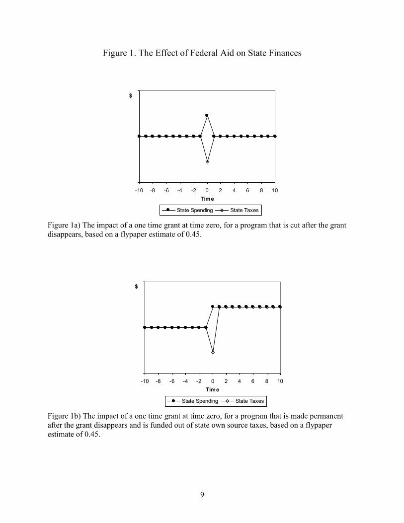
Figure 1. The Effect of Federal Aid on State Finances

-10 -8 -6 -4 -2 0 2 4 6 8 10

Time

$

State Spending State Taxes

Figure 1a) The impact of a one time grant at time zero, for a program that is cut after the grant

disappears, based on a flypaper estimate of 0.45.

-10 -8 -6 -4 -2 0 2 4 6 8 10

Time

$

State Spending State Taxes

Figure 1b) The impact of a one time grant at time zero, for a program that is made permanent

after the grant disappears and is funded out of state own source taxes, based on a flypaper

estimate of 0.45.

10

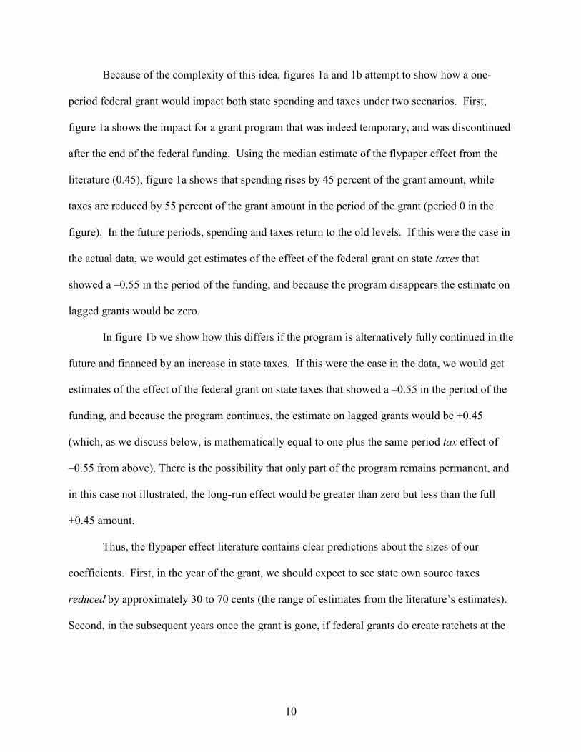
Because of the complexity of this idea, figures 1a and 1b attempt to show how a one-

period federal grant would impact both state spending and taxes under two scenarios. First,

figure 1a shows the impact for a grant program that was indeed temporary, and was discontinued

after the end of the federal funding. Using the median estimate of the flypaper effect from the

literature (0.45), figure 1a shows that spending rises by 45 percent of the grant amount, while

taxes are reduced by 55 percent of the grant amount in the period of the grant (period 0 in the

figure). In the future periods, spending and taxes return to the old levels. If this were the case in

the actual data, we would get estimates of the effect of the federal grant on state taxes that

showed a –0.55 in the period of the funding, and because the program disappears the estimate on

lagged grants would be zero.

In figure 1b we show how this differs if the program is alternatively fully continued in the

future and financed by an increase in state taxes. If this were the case in the data, we would get

estimates of the effect of the federal grant on state taxes that showed a –0.55 in the period of the

funding, and because the program continues, the estimate on lagged grants would be +0.45

(which, as we discuss below, is mathematically equal to one plus the same period tax effect of

–0.55 from above). There is the possibility that only part of the program remains permanent, and

in this case not illustrated, the long-run effect would be greater than zero but less than the full

+0.45 amount.

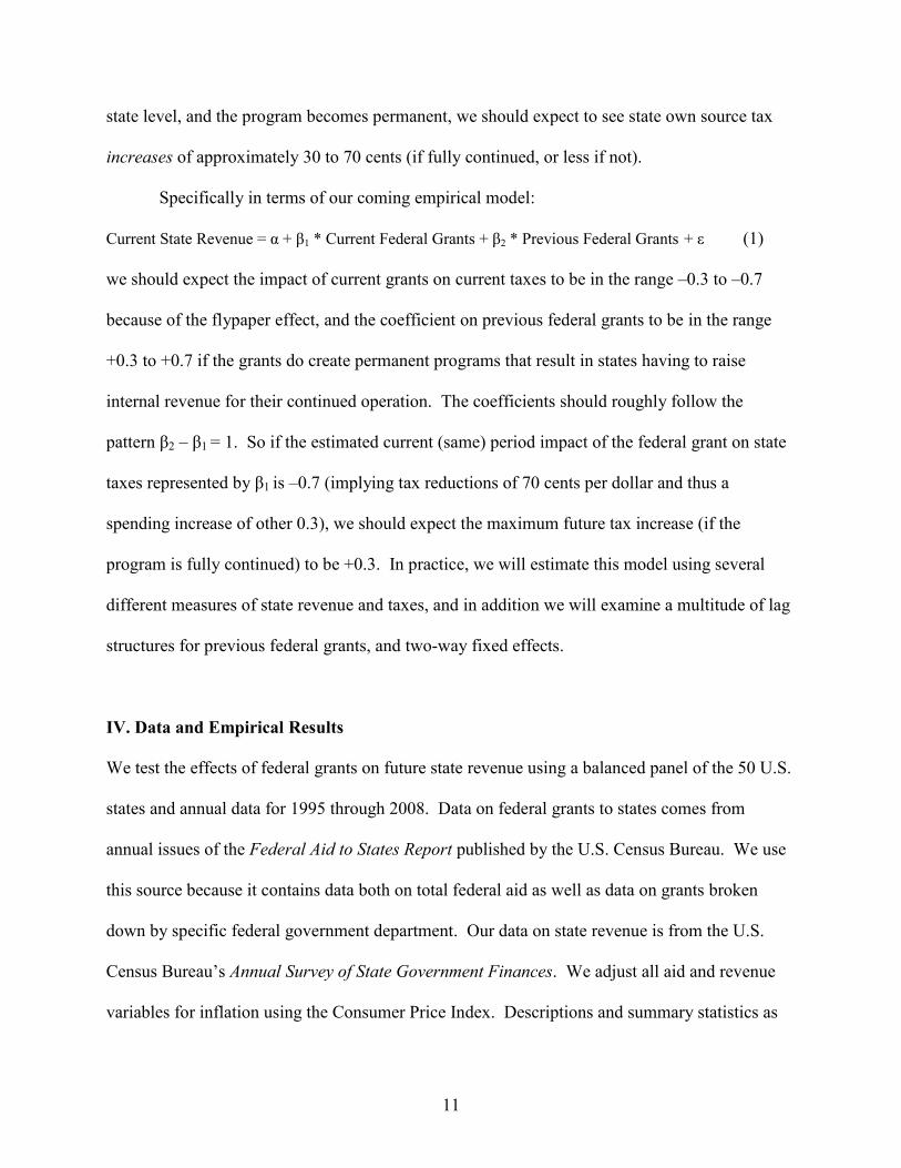
Thus, the flypaper effect literature contains clear predictions about the sizes of our

coefficients. First, in the year of the grant, we should expect to see state own source taxes

reduced by approximately 30 to 70 cents (the range of estimates from the literature‘s estimates).

Second, in the subsequent years once the grant is gone, if federal grants do create ratchets at the

11

state level, and the program becomes permanent, we should expect to see state own source tax

increases of approximately 30 to 70 cents (if fully continued, or less if not).

Specifically in terms of our coming empirical model:

Current State Revenue = α + β1 * Current Federal Grants + β2 * Previous Federal Grants + ε (1)

we should expect the impact of current grants on current taxes to be in the range –0.3 to –0.7

because of the flypaper effect, and the coefficient on previous federal grants to be in the range

+0.3 to +0.7 if the grants do create permanent programs that result in states having to raise

internal revenue for their continued operation. The coefficients should roughly follow the

pattern β2 – β1 = 1. So if the estimated current (same) period impact of the federal grant on state

taxes represented by β1 is –0.7 (implying tax reductions of 70 cents per dollar and thus a

spending increase of other 0.3), we should expect the maximum future tax increase (if the

program is fully continued) to be +0.3. In practice, we will estimate this model using several

different measures of state revenue and taxes, and in addition we will examine a multitude of lag

structures for previous federal grants, and two-way fixed effects.

IV. Data and Empirical Results

We test the effects of federal grants on future state revenue using a balanced panel of the 50 U.S.

states and annual data for 1995 through 2008. Data on federal grants to states comes from

annual issues of the Federal Aid to States Report published by the U.S. Census Bureau. We use

this source because it contains data both on total federal aid as well as data on grants broken

down by specific federal government department. Our data on state revenue is from the U.S.

Census Bureau‘s Annual Survey of State Government Finances. We adjust all aid and revenue

variables for inflation using the Consumer Price Index. Descriptions and summary statistics as

12

well as a complete list of data sources for all variables used in this paper can be found in

appendix 1.

Our panel data allows for the estimation of two-way fixed effects models. The use of

two-way fixed effects controls for all factors that are either specific to a state through time (such

as a given state having a smaller budget due to not having an income tax, for example) or

common across all states in a given time period of data (such as a national economic recession,

for example) and is preferable to attempting to control for a host of other factors that can affect

own source revenue.7 This, of course, prevents us from using the traditional demographic

controls (such as median age or percent nonwhite) as these factors do not vary enough through

time in a given state, and are thus picked up by the state fixed effects. We estimate our fixed

effect regressions with ordinary least squares. After incorporating several lags of our federal aid

variable our number of usable observations becomes 400, spanning the period 2001–2008.

Our basic empirical model is one in which we use state own source revenue as the

dependent variable, and our independent variables of interest are current and previous federal

grants. Our biggest challenge is formulating the best lag structure for previous federal grants.

We begin by including only current period federal grants and a one-year lag, and then add

additional lagged federal grants one period at a time.8 We present the results of this experiment

in table 1.

13

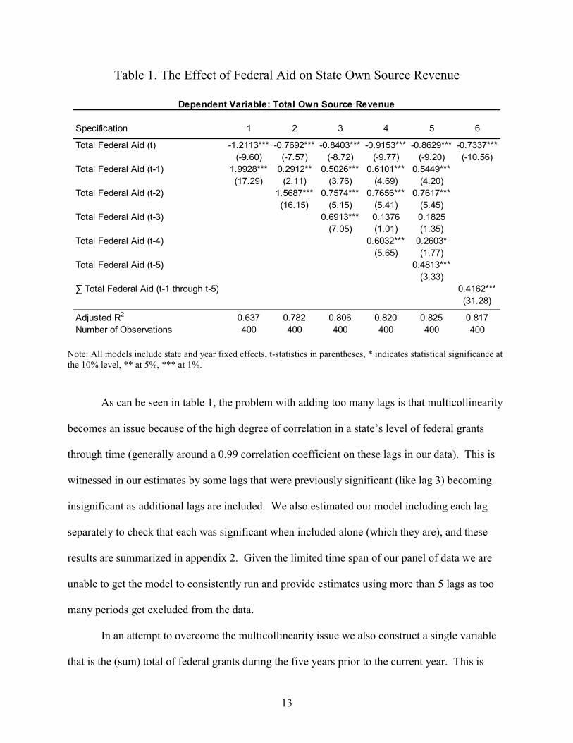
Table 1. The Effect of Federal Aid on State Own Source Revenue

Specification 1 2 3 4 5 6

Total Federal Aid (t) -1.2113*** -0.7692*** -0.8403*** -0.9153*** -0.8629*** -0.7337***

(-9.60) (-7.57) (-8.72) (-9.77) (-9.20) (-10.56)

Total Federal Aid (t-1) 1.9928*** 0.2912** 0.5026*** 0.6101*** 0.5449***

(17.29) (2.11) (3.76) (4.69) (4.20)

Total Federal Aid (t-2) 1.5687*** 0.7574*** 0.7656*** 0.7617***

(16.15) (5.15) (5.41) (5.45)

Total Federal Aid (t-3) 0.6913*** 0.1376 0.1825

(7.05) (1.01) (1.35)

Total Federal Aid (t-4) 0.6032*** 0.2603*

(5.65) (1.77)

Total Federal Aid (t-5) 0.4813***

(3.33)

∑ Total Federal Aid (t-1 through t-5) 0.4162***

(31.28)

Adjusted R2 0.637 0.782 0.806 0.820 0.825 0.817

Number of Observations 400 400 400 400 400 400

Dependent Variable: Total Own Source Revenue

Note: All models include state and year fixed effects, t-statistics in parentheses, * indicates statistical significance at

the 10% level, ** at 5%, *** at 1%.

As can be seen in table 1, the problem with adding too many lags is that multicollinearity

becomes an issue because of the high degree of correlation in a state‘s level of federal grants

through time (generally around a 0.99 correlation coefficient on these lags in our data). This is

witnessed in our estimates by some lags that were previously significant (like lag 3) becoming

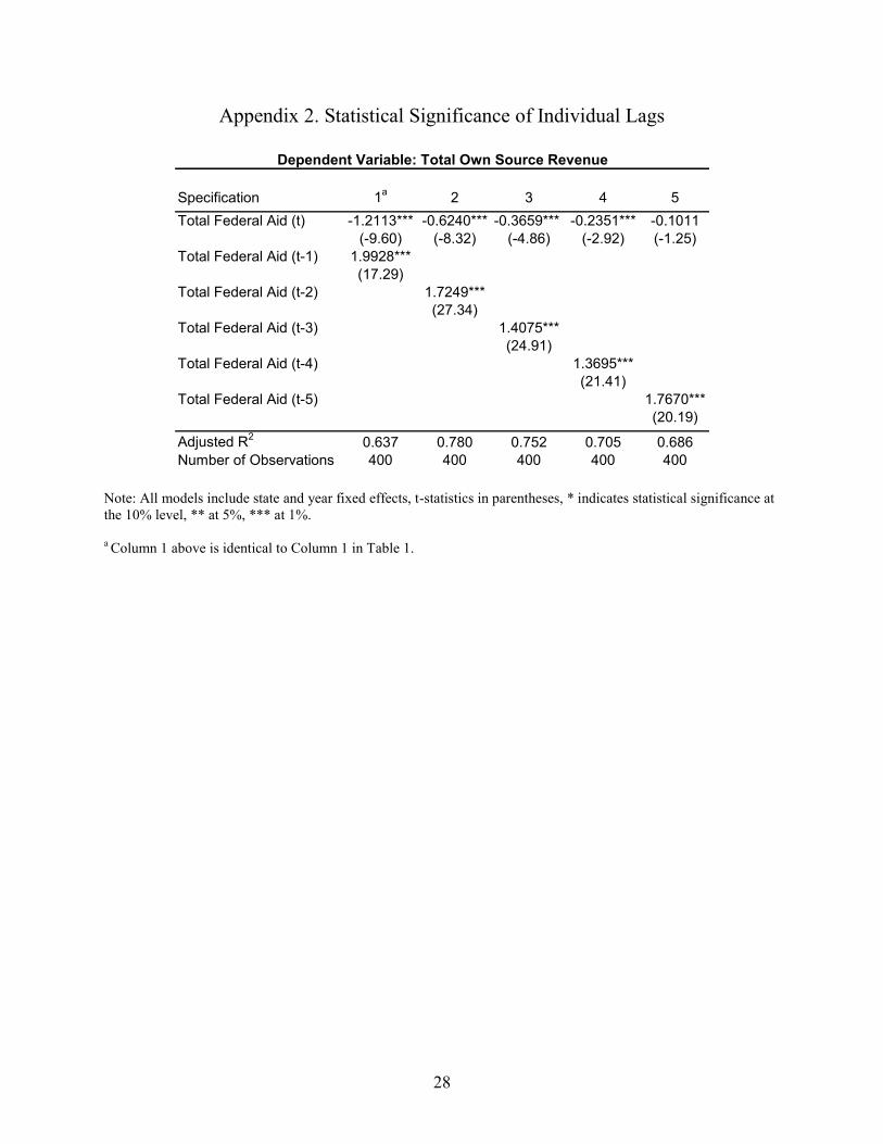
insignificant as additional lags are included. We also estimated our model including each lag

separately to check that each was significant when included alone (which they are), and these

results are summarized in appendix 2. Given the limited time span of our panel of data we are

unable to get the model to consistently run and provide estimates using more than 5 lags as too

many periods get excluded from the data.

In an attempt to overcome the multicollinearity issue we also construct a single variable

that is the (sum) total of federal grants during the five years prior to the current year. This is

14

presented in the final column of table 1. This is our most ―clean‖ specification and, interestingly,

also produces some of the most reasonable estimates based on our prior expectations. Not only

is the single coefficient on the cumulative total fairly representative of the average coefficient on

the individual lags in the previous columns, but more importantly the estimates in this final

specification roughly satisfy the linear relationship β2 – β1 = 1 that was anticipated from the

literature [+0.4162 – (–0.7337) = 1.1499], and we cannot statistically reject the hypothesis that

the sum is indeed one (the implied 95 percent confidence interval is 0.99 to 1.30).9

Most importantly, however is the fact that the estimates suggest a full permanent

programmatic effect with future taxes being roughly the amount required to permanently expand

spending by the amount caused initially by the federal grant. In all specifications there is a clear

positive effect of federal grants on the future tax levels in a state, even going back in time up to 5

or more lags. These results seem to confirm our hypothesis.

15

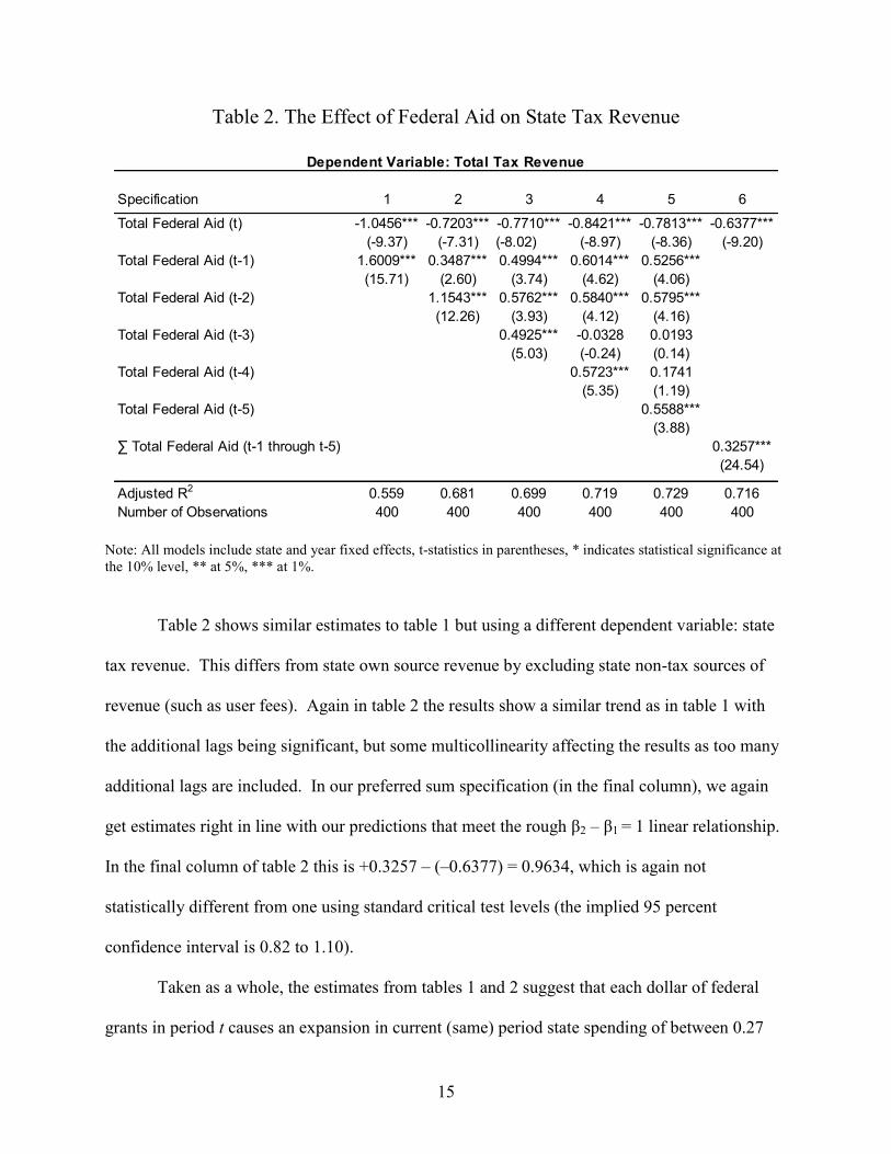
Table 2. The Effect of Federal Aid on State Tax Revenue


Total Federal Aid (t) -1.0456*** -0.7203*** -0.7710*** -0.8421*** -0.7813*** -0.6377***

(-9.37) (-7.31) (-8.02) (-8.97) (-8.36) (-9.20)

Total Federal Aid (t-1) 1.6009*** 0.3487*** 0.4994*** 0.6014*** 0.5256***

(15.71) (2.60) (3.74) (4.62) (4.06)

Total Federal Aid (t-2) 1.1543*** 0.5762*** 0.5840*** 0.5795***

(12.26) (3.93) (4.12) (4.16)

Total Federal Aid (t-3) 0.4925*** -0.0328 0.0193

(5.03) (-0.24) (0.14)

Total Federal Aid (t-4) 0.5723*** 0.1741

(5.35) (1.19)


(3.88)

∑ Total Federal Aid (t-1 through t-5) 0.3257***

(24.54)

Adjusted R2 0.559 0.681 0.699 0.719 0.729 0.716


Dependent Variable: Total Tax Revenue


the 10% level, ** at 5%, *** at 1%.

Table 2 shows similar estimates to table 1 but using a different dependent variable: state

tax revenue. This differs from state own source revenue by excluding state non-tax sources of

revenue (such as user fees). Again in table 2 the results show a similar trend as in table 1 with

the additional lags being significant, but some multicollinearity affecting the results as too many

additional lags are included. In our preferred sum specification (in the final column), we again

get estimates right in line with our predictions that meet the rough β2 – β1 = 1 linear relationship.

In the final column of table 2 this is +0.3257 – (–0.6377) = 0.9634, which is again not

statistically different from one using standard critical test levels (the implied 95 percent

confidence interval is 0.82 to 1.10).

Taken as a whole, the estimates from tables 1 and 2 suggest that each dollar of federal

grants in period t causes an expansion in current (same) period state spending of between 0.27

16

and 0.36 (in the lower range of the previous flypaper literature estimates, and this is calculated as

1- β1), and then subsequently results in states raising taxes by between 0.33 and 0.42 (this is

simply β2) which is precisely the amount required to permanently continue all of the state

programs created through the initial federal grants.

While this should be obvious based on our discussion of figures 1a and 1b, it is worth

clarifying that this is not simply a case where the grant is used to cut taxes in the current period

and then taxes are raised back to their previous levels after the grant. The grant results in

permanently larger state government spending that must be financed by permanently higher

levels of own source taxation. Because of how it is specified, our estimate of future tax increases

is the marginal amount by which future taxes are higher than they would have been without the

grant ever taking place, meaning the true tax increases in the year the grant disappears are larger

than this estimate as taxes must be increased both to replace the one-year partial tax cut in the

period of the grant and additionally to fund the expansion in programmatic spending.

Of note is the fact that the adjusted R-squared values are uniformly higher for the

specifications using own source revenue than they are for the specifications using tax revenue.

Because the difference is that own source includes other non-tax sources of revenue (such as user

charges and fees), this result may imply that changes in these other non-tax sources of revenue

for states are slightly easier to accomplish and are an important part of how states adjust their

own revenue in response to federal grants.

V. Grant Analysis by Department

Federal grants to states are given through individual federal government agencies. The five

agencies which provide the largest amount of grants are the Department of Health and Human

17

Services (accounting for 57.0 percent of grants), Department of Transportation (11.3 percent of

grants), Department of Housing and Urban Development (10.1 percent of grants), Department of

Education (7.7 percent of grants), and Department of Agriculture (5.9 percent of grants).10

Combined, these five largest grant areas account for 92 percent of all federal grants. In this

section we explore the question of whether grants from different government agencies tend to

have different degrees of permanence or, more precisely, different degrees of impact on future

state taxes.

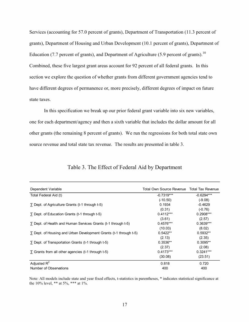
In this specification we break up our prior federal grant variable into six new variables,

one for each department/agency and then a sixth variable that includes the dollar amount for all

other grants (the remaining 8 percent of grants). We run the regressions for both total state own

source revenue and total state tax revenue. The results are presented in table 3.

Table 3. The Effect of Federal Aid by Department

Dependent Variable Total Own Source Revenue Total Tax Revenue

Total Federal Aid (t) -0.7319*** -0.6294***

(-10.50) (-9.08)

∑ Dept. of Agriculture Grants (t-1 through t-5) 0.1934 -0.4629

(0.31) (-0.76)

∑ Dept. of Education Grants (t-1 through t-5) 0.4112*** 0.2908***

(3.61) (2.57)

∑ Dept. of Health and Human Services Grants (t-1 through t-5) 0.4576*** 0.3639***

(10.03) (8.02)

∑ Dept. of Housing and Urban Development Grants (t-1 through t-5) 0.5422** 0.5932**

(2.13) (2.35)

∑ Dept. of Transportation Grants (t-1 through t-5) 0.3536** 0.3095**

(2.37) (2.08)

∑ Grants from all other agencies (t-1 through t-5) 0.4173*** 0.3241***

(30.08) (23.51)

Adjusted R2 0.818 0.720

Number of Observations 400 400


the 10% level, ** at 5%, *** at 1%.

18

Interestingly, four of the six coefficients are almost identical. The coefficients for

Department of Education, Department of Health and Human Services, Department of

Transportation, and all other federal grants are all positive and significant, and roughly in the

range of 0.35 to 0.46 in the own source revenue specifications and in the range of 0.29 to 0.36 in

the tax revenue specifications. Grants from the Department of Housing and Urban Development

in both specifications have the highest long-run impact on taxes at 0.54 in own source and 0.59

in tax revenue. All of these estimates are roughly in the range suggested by the linear flypaper

rule, and the results imply that virtually the entire bump in program spending continues into the

future to be financed through state internal taxes. Also interestingly, the highest-to-lowest

ranking of the coefficients across departments is identical in the two specifications, although the

coefficients in the tax revenue specifications tend to be slightly smaller (with the exception of the

Department of Housing and Development).

The coefficient on the Department of Agriculture is the only one whose results seem to

be at odds with the other results, with a coefficient of 0.19 that is the right sign but insignificant

in the own source specification (although, interestingly, also not significantly different from the

value of 0.2681 implied by the linear relationship) and a coefficient of -0.46 that is the wrong

sign but insignificant in the tax revenue specification. We are unsure why the results from this

one agency are different from the other results. Whether grants from the Department of

Agriculture truly carry less long-run burden on states, or whether this is a spurious estimate due

to the multicollinearity among the grants is unclear. Given that the coefficient is not statistically

different from either zero or the predicted value in the own source specification, we are reluctant

to draw firm conclusions that grants from this one agency are somehow different. This is

particularly true given that the other four not only have common estimates, but are also in line

19

with the estimate from the all other grants variable. In addition, of the five largest grant agencies

we have singled out, the Department of Agriculture accounts for the smallest percentage of

grants. Thus, we think the most likely conclusion that can be reached is that there are not large

differences in the long-run persistence of grants across agencies.

Also worthy of note is that again in these regressions, the specification using own source

has a higher adjusted R-squared than the specification using tax revenue, supporting the idea that

these non-tax adjustments in revenue are an important factor in explaining how states respond to

federal grants.

VI. Individual Revenue Source Estimations

In this section we attempt to more precisely test our hypothesis by directly examining the effect

of federal grants on individual state tax rates. Based on the results of the last section, we return

to a combined variable reflecting total grants rather than breaking it out by agency.

For each state we are able to collect individual tax rates for the state sales tax, the state

cigarette tax, and the state beer tax. Most state personal and corporate income taxes have bracket

structures with different rates, making it impossible to use one specific tax rate, so in an effort to

include them we have instead used state personal and corporate income tax revenue rather than

rates. The results of our estimations are summarized in table 4.

20

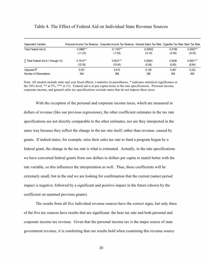
Table 4. The Effect of Federal Aid on Individual State Revenue Sources

Dependent Variable Personal Income Tax Revenue Corporate Income Tax Revenue General Sales Tax Rate Cigarette Tax Rate Beer Tax Rate

Total Federal Aid (t) -0.5866*** -0.1145*** -0.00002 -0.0166 -0.0003***

(-11.23) (-7.93) (-0.10) (-0.92) (-6.33)

∑ Total Federal Aid (t-1 through t-5) 0.1514*** 0.0531*** 0.00001 0.0038 0.0001***

(15.30) (19.40) (0.06) (0.65) (8.84)

Adjusted R2 0.521 0.615 0.128 0.467 0.223

Number of Observations 344 368 360 400 400


the 10% level, ** at 5%, *** at 1%. Federal aid is in per capita terms in the rate specifications. Personal income,

corporate income, and general sales tax specifications exclude states that do not impose these taxes.

With the exception of the personal and corporate income taxes, which are measured in

dollars of revenue (like our previous regressions), the other coefficient estimates in the tax rate

specifications are not directly comparable to the other estimates, nor are they interpreted in the

same way because they reflect the change in the tax rate itself, rather than revenue, caused by

grants. If indeed states, for example, raise their sales tax rate to fund a program begun by a

federal grant, the change in the tax rate is what is estimated. Actually, in the rate specifications

we have converted federal grants from raw dollars to dollars per capita to match better with the

rate variable, so this influences the interpretation as well. Thus, these coefficients will be

extremely small, but in the end we are looking for confirmation that the current (same) period

impact is negative, followed by a significant and positive impact in the future (shown by the

coefficient on summed previous grants).

The results from all five individual revenue sources have the correct signs, but only three

of the five tax sources have results that are significant: the beer tax rate and both personal and

corporate income tax revenue. Given that the personal income tax is the major source of state

government revenue, it is comforting that our results hold when examining this revenue source

21

directly. Although it is disappointing that we cannot see the results being more significant for

state sales taxes, which are also a major revenue source, this may simply imply states rely more

on income taxes and other revenue sources when adjusting to changes in federal aid.

VII. Do Federal and State Grants Create Ratchets in Local Taxes?

In theory, this permanent impact of grants should also apply at the local level. Local

governments not only receive grants from the federal government, but also from state

government as well. Here we examine whether federal and state grants to localities have similar

impacts on future local taxes.

We focus our analysis of local governments on a case study of counties in Pennsylvania

for which we were able to obtain detailed grant information. Our data cover 63 counties

annually over the period 1997 to 2004. The panel includes federal and state aid as well as data

on total own source revenue for each county. After including lagged federal and state aid data,

our Pennsylvania county panel consists of 252 total observations and spans the period 2001 to

2004. Aid and revenue variables are again adjusted for inflation using the Consumer Price

Index. Summary statistics, descriptions, and sources for these variables can also be found in

appendix 1.

As before, we employ a two-way fixed effects model. Again, the use of fixed effects

helps control for omitted variables which are either constant through time for all counties or

specific to a single county. Since our data on Pennsylvania counties contains substantially fewer

years than our state-level data we must use fewer lags in our models.

For our local analysis we focus only on total own source revenue and do not specifically

attempt to model individual taxes. For states, tax revenue is 71 percent of all own source

22

revenue, but for our local governments in the sample, tax revenue accounts for only 43 percent of

all own source revenue. Local governments rely much more heavily on non-tax revenue sources

such as license and user fees and the total own source revenue would include these but tax

revenue would not. We also note that even for states, the specifications using own source

revenue had a higher adjusted R-squared.

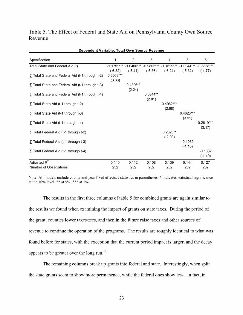
We begin our analysis by including current and lagged grant variables that reflect the

total grants received by the county (combined state and federal grants). We will then break this

into two variables to see if we can find differences in the effect of state versus federal grants on

county taxation. The first three columns of table 5 show the results of our estimations using

combined grants to county governments in Pennsylvania. We show how the results change as

we change the length of the historical sum. The first column, for example, contains a variable

that is two periods of lagged grants, while the second column of results is for three periods of

grants, and so forth.

23

Table 5. The Effect of Federal and State Aid on Pennsylvania County Own Source

Revenue


Total State and Federal Aid (t) -1.1751*** -1.0400*** -0.9802*** -1.1629*** -1.0044*** -0.8838***

(-6.32) (-5.41) (-5.36) (-6.24) (-5.32) (-4.77)

∑ Total State and Federal Aid (t-1 through t-2) 0.3068***

(3.63)

∑ Total State and Federal Aid (t-1 through t-3) 0.1396**

(2.24)

∑ Total State and Federal Aid (t-1 through t-4) 0.0844**

(2.01)

∑ Total State Aid (t-1 through t-2) 0.4062***

(2.98)


(3.91)


(3.17)

∑ Total Federal Aid (t-1 through t-2) 0.2323**

(-2.00)

∑ Total Federal Aid (t-1 through t-3) -0.1089

(-1.10)

∑ Total Federal Aid (t-1 through t-4) -0.1382

(-1.40)

Adjusted R2 0.140 0.112 0.108 0.139 0.144 0.127



Note: All models include county and year fixed effects, t-statistics in parentheses, * indicates statistical significance

at the 10% level, ** at 5%, *** at 1%.

The results in the first three columns of table 5 for combined grants are again similar to

the results we found when examining the impact of grants on state taxes. During the period of

the grant, counties lower taxes/fees, and then in the future raise taxes and other sources of

revenue to continue the operation of the programs. The results are roughly identical to what was

found before for states, with the exception that the current period impact is larger, and the decay

appears to be greater over the long run.11

The remaining columns break up grants into federal and state. Interestingly, when split

the state grants seem to show more permanence, while the federal ones show less. In fact, in

24

some of the specifications, the lagged federal grant variable becomes negative and insignificant.

We are unsure why this is the case, but note this is clearly why in the combined grant variable it

begins to diminish, as by itself the state variable doesn‘t decline as much as additional lags are

added. In theory there is no reason why state and federal grants should function differently. We

do note that the federal grants are much smaller than state grants to local governments.

Approximately three-fourths of all grants to local governments come in the form of state

grants (in our sample). So the state results are relatively more important. In addition, we are

only examining county governments in one state, and it is unclear if these results would hold up

for other levels of local government (cities or school districts, for example), or for other states.

Nonetheless, when we examine either the combined grants or the state grants, the results

for local governments seem to mirror our results from earlier. For every $100 in grants, local

governments eventually raise revenue by between $23 and $46 to support the continued

operation of these programs.

VIII. Conclusion

While a vast previous literature has examined the impact of federal grants on state and local

spending, this previous literature focuses exclusively on the impact of the grant in the period it is

received. We depart from this literature by examining the impact of federal grants on state and

local tax policy in future periods.

Our results clearly demonstrate that grant funding to state and local governments results

in higher own source revenue and taxes in the future to support the programs initiated with the

federal grant monies. Our results are consistent with Friedman‘s quote regarding the

permanence of temporary government programs started through grant funding, as well as South

25

Carolina Governor Mark Sanford‘s reasoning for trying to deny some federal stimulus monies

for his state due to the future tax implications. Most importantly, our results suggest that the

recent large increase in federal grants to state and local governments that has occurred as part of

the American Recovery and Reinvestment Act (ARRA) will have significant future tax

implications at the state and local level as these governments raise revenue to continue these

newly funded programs into the future. Federal grants to state and local governments have risen

from $461 billion in 2008 to $654 billion in 2010. Based on our estimates, future state taxes will

rise by between 33 and 42 cents for every dollar in federal grants states received today, while

local revenues will rise by between 23 and 46 cents for every dollar in federal (or state) grants

received today. Using our estimates, this increase of $200 billion in federal grants will eventually

result in roughly $80 billion in future state and local tax and own source revenue increases. This

suggests the true cost of fiscal stimulus is underestimated when the costs of future state and local

tax increases are overlooked.

1 The original Friedman quote appears both in the October 27

th, 2993 issue of the Cleveland Plain Dealer and in the

book he coauthored with his wife Rose D. Friedman, Tyranny of the Status Quo (Harourt Brace Jovanovich, San

Diego, CA, 1984, pg. 115). Variants of this quote have also been attributed to President Ronald Reagan and Utah

Senator Wallace F. Bennett. Reagan‘s quote is ―We have long since discovered that nothing lasts longer than a

temporary government program,‖ appearing in Ronald Reagan: The Great Communicator (HarperPerennial, New

York, NY, 2001, pg. 59). Bennett‘s quote is ―It is an age-old Washington axiom that there is nothing so permanent

as a temporary government program,‖ appearing (somewhat ironically given the topic of our paper) in a government

committee review of federal grants to states (Periodic Congressional Review of Federal Grants-in-aid, published by

United States Congress, Senate, Committee on Government Operations, 1964, pg. 15). 2 See Higgs (1987), chapter 8, for a discussion of the many remaining ‗institutional legacies‘ of the New Deal

programs. 3 The ‗leviathan‘ model of government is one that assumes the objective of government is to maximize its size, see

Brennan and Buchanan (1977, 1978, 1980). 4 Rent seeking is the term used to refer to the expenditure of resources to capture political transfers, see Tullock

(1967). 5 In the terminology of Baumol (1990), the expansion of government spending increases the return to unproductive

entrepreneurship. See Coyne, Sobel, Dove (forthcoming) for a discussion of how this industry specific (lobbying)

capital does not easily transfer back into the private sector. 6 In this section we provide only a brief summary of the main arguments in this rather large literature. See Hines

and Thaler (1995) and Bailey and Connolly (1998) for excellent overviews and summaries of this large empirical

literature and the theoretical expectations. 7 We experimented with the inclusion of state-specific time trends in addition to state fixed effects. None of the

state trend variables were statistically significant, indicating our two-way, state and year, fixed effects are sufficient.

26

8 We have adjusted for the difference between federal and state fiscal years in the data by pre-lagging federal funds

by one year. 9 One can back out the implied flypaper effect coefficients (on spending) from our regressions (on taxes) for

comparison with previous literature by calculating 1- β1, which is 0.2663 in the final specification. 10

Percentages are for federal grants to state and local governments for federal fiscal year 2008. 11

In theory, the maximum coefficient on the current period is one, and in the table some of the coefficients are

greater than one, however, none of these are significantly different from one at traditional levels.

27

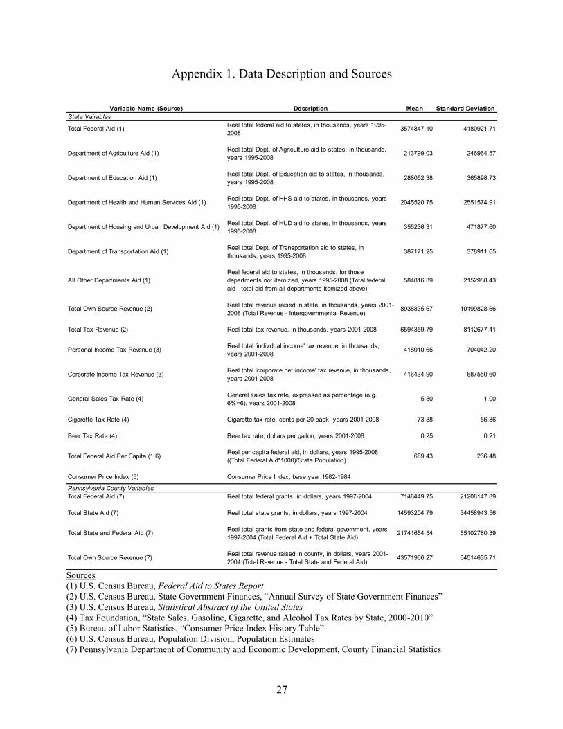
Appendix 1. Data Description and Sources

Variable Name (Source) Description Mean Standard Deviation

State Vairables

Total Federal Aid (1)Real total federal aid to states, in thousands, years 1995-

20083574847.10 4180921.71

Department of Agriculture Aid (1)Real total Dept. of Agriculture aid to states, in thousands,

years 1995-2008213799.03 246964.57

Department of Education Aid (1)Real total Dept. of Education aid to states, in thousands,

years 1995-2008288052.38 365898.73

Department of Health and Human Services Aid (1)Real total Dept. of HHS aid to states, in thousands, years

1995-20082045520.75 2551574.91

Department of Housing and Urban Development Aid (1)Real total Dept. of HUD aid to states, in thousands, years

1995-2008355236.31 471877.60

Department of Transportation Aid (1)Real total Dept. of Transportation aid to states, in

thousands, years 1995-2008387171.25 378911.65

All Other Departments Aid (1)

Real federal aid to states, in thousands, for those

departments not itemized, years 1995-2008 (Total federal

aid - total aid from all departments itemized above)

584816.39 2152988.43

Total Own Source Revenue (2)Real total revenue raised in state, in thousands, years 2001-

2008 (Total Revenue - Intergovernmental Revenue)8938835.67 10199828.66

Total Tax Revenue (2) Real total tax revenue, in thousands, years 2001-2008 6594359.79 8112677.41

Personal Income Tax Revenue (3)Real total 'individual income' tax revenue, in thousands,

years 2001-2008418010.65 704042.20

Corporate Income Tax Revenue (3)Real total 'corporate net income' tax revenue, in thousands,

years 2001-2008416434.90 687550.60

General Sales Tax Rate (4)General sales tax rate, expressed as percentage (e.g.

6%=6), years 2001-20085.30 1.00

Cigarette Tax Rate (4) Cigarette tax rate, cents per 20-pack, years 2001-2008 73.88 56.86

Beer Tax Rate (4) Beer tax rate, dollars per gallon, years 2001-2008 0.25 0.21

Total Federal Aid Per Capita (1,6)Real per capita federal aid, in dollars, years 1995-2008

((Total Federal Aid*1000)/State Population)689.43 266.48

Consumer Price Index (5) Consumer Price Index, base year 1982-1984

Pennsylvania County Variables

Total Federal Aid (7) Real total federal grants, in dollars, years 1997-2004 7148449.75 21208147.89

Total State Aid (7) Real total state grants, in dollars, years 1997-2004 14593204.79 34458943.56

Total State and Federal Aid (7)Real total grants from state and federal government, years

1997-2004 (Total Federal Aid + Total State Aid)21741654.54 55102780.39

Total Own Source Revenue (7)Real total revenue raised in county, in dollars, years 2001-

2004 (Total Revenue - Total State and Federal Aid)43571966.27 64514635.71

Sources

(1) U.S. Census Bureau, Federal Aid to States Report

(2) U.S. Census Bureau, State Government Finances, ―Annual Survey of State Government Finances‖

(3) U.S. Census Bureau, Statistical Abstract of the United States

(4) Tax Foundation, ―State Sales, Gasoline, Cigarette, and Alcohol Tax Rates by State, 2000-2010‖

(5) Bureau of Labor Statistics, ―Consumer Price Index History Table‖

(6) U.S. Census Bureau, Population Division, Population Estimates

(7) Pennsylvania Department of Community and Economic Development, County Financial Statistics

28

Appendix 2. Statistical Significance of Individual Lags

Specification 1a

2 3 4 5

Total Federal Aid (t) -1.2113*** -0.6240*** -0.3659*** -0.2351*** -0.1011

(-9.60) (-8.32) (-4.86) (-2.92) (-1.25)


(17.29)


(27.34)


(24.91)


(21.41)


(20.19)

Adjusted R2

0.637 0.780 0.752 0.705 0.686

Number of Observations 400 400 400 400 400



the 10% level, ** at 5%, *** at 1%.

a Column 1 above is identical to Column 1 in Table 1.

29

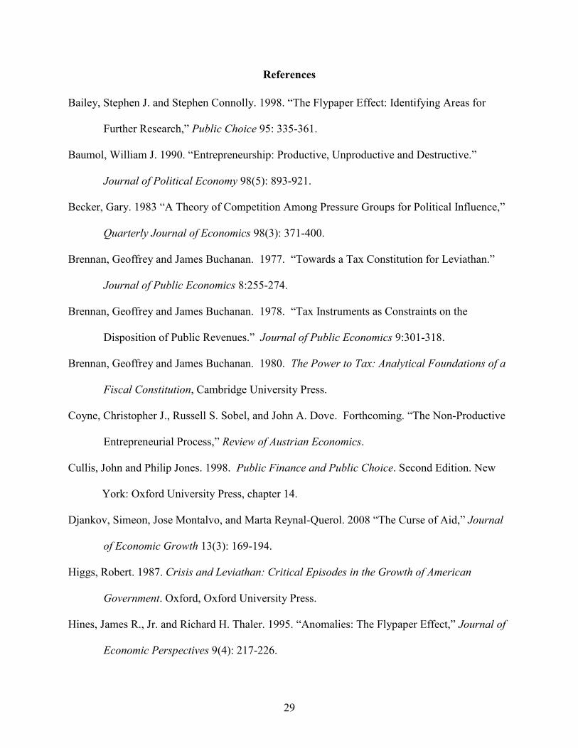
References

Bailey, Stephen J. and Stephen Connolly. 1998. ―The Flypaper Effect: Identifying Areas for

Further Research,‖ Public Choice 95: 335-361.

Baumol, William J. 1990. ―Entrepreneurship: Productive, Unproductive and Destructive.‖

Journal of Political Economy 98(5): 893-921.

Becker, Gary. 1983 ―A Theory of Competition Among Pressure Groups for Political Influence,‖

Quarterly Journal of Economics 98(3): 371-400.

Brennan, Geoffrey and James Buchanan. 1977. ―Towards a Tax Constitution for Leviathan.‖

Journal of Public Economics 8:255-274.

Brennan, Geoffrey and James Buchanan. 1978. ―Tax Instruments as Constraints on the

Disposition of Public Revenues.‖ Journal of Public Economics 9:301-318.

Brennan, Geoffrey and James Buchanan. 1980. The Power to Tax: Analytical Foundations of a

Fiscal Constitution, Cambridge University Press.

Coyne, Christopher J., Russell S. Sobel, and John A. Dove. Forthcoming. ―The Non-Productive

Entrepreneurial Process,‖ Review of Austrian Economics.

Cullis, John and Philip Jones. 1998. Public Finance and Public Choice. Second Edition. New

York: Oxford University Press, chapter 14.

Djankov, Simeon, Jose Montalvo, and Marta Reynal-Querol. 2008 ―The Curse of Aid,‖ Journal

of Economic Growth 13(3): 169-194.

Higgs, Robert. 1987. Crisis and Leviathan: Critical Episodes in the Growth of American

Government. Oxford, Oxford University Press.

Hines, James R., Jr. and Richard H. Thaler. 1995. ―Anomalies: The Flypaper Effect,‖ Journal of

Economic Perspectives 9(4): 217-226.

30

Leeson, Peter T., and Russell S. Sobel. 2008. ―Weathering Corruption,‖ Journal of Law and

Economics 51(4): 667-681

Musgrave, Richard. 1981. ―Leviathan Cometh—Or Does He?‖ in H. Ladd and T. N. Tiedman

(eds.) Tax and Expenditure Limitations, COUPE Papers on Public Economics, 5,

Washington, DC: The Urban Institute, 77-120.

Tullock, Gordon. 1967. ―The Welfare Cost of Tariffs, Monopolies, and Theft,‖ Western

Economic Journal 5(3): 224-232.

Weingast, Barry R., Kenneth A. Shepsle, and Christopher Johnsen. 1981. ―The Political

Economy of Benefits and Costs: A Neoclassical Approach to Distributive Politics,‖

Journal of Political Economy 89(4): 642-664.

Documents

august 2010 working paper - Mercatus Center