Auditing: A Journal of Practice & Theory American

Auditing: A Journal of Practice & Theory American Accounting AssociationVol. 31, No. 2 DOI: 10.2308/ajpt-10241May 2012pp. 43–72

Geographic Proximity between Auditor andClient: How Does It Impact Audit Quality?

Jong-Hag Choi, Jeong-Bon Kim, Annie A. Qiu, and Yoonseok Zang

SUMMARY: Using a large sample of audit client firms, this paper investigates whether

and how the geographic proximity between auditor and client affects audit quality proxied

by accrual-based earnings quality. We define an auditor as a local auditor (1) if the

auditor’s practicing office is located in the same metropolitan statistical area (MSA) as

the client’s headquarters, and (2) if the geographic distance between the two cities where

the auditor’s practicing office and the client’s headquarters are located is within 100

kilometers, or they are in the same MSA. As predicted, our empirical results are

consistent with local auditors providing higher-quality audit services than non-local

auditors. In addition, as predicted, this quality difference is weakened for diversified

clients with more operating or geographic segments. The results are robust to a variety

of sensitivity checks. Overall, our evidence suggests that informational advantages

associated with local audits enable auditors to better constrain management’s biased

earnings reporting, with greater advantages for less diversified clients.

Keywords: auditor locality; geographic proximity; audit quality; diversification.

JEL Classification: M42.

INTRODUCTION

Since the Enron debacle and the subsequent collapse of Arthur Andersen, regulators,

lawmakers, academic researchers, and the popular press have paid considerable attention to

engagement-specific factors determining the auditor-client relationship and their impact on

Jong-Hag Choi is an Associate Professor at Seoul National University, Jeong-Bon Kim is a Chair Professor atCity University of Hong Kong, Annie A. Qiu is Head of the International Business Department at CITICSecurities Co., Ltd., Beijing, and Yoonseok Zang is an Associate Professor at Singapore Management University.

We appreciate the helpful comments of Charles Chen, Sunhwa Choi, Shifei Chung, Chris Hogan (editor), Lee-SeokHwang, Akira Kanie, Bin Ke, Soo Young Kwon, Jay Junghun Lee, Akihiro Noguchi, Jaime Schmidt, Haina Shi, ByronSong, Joon Yong Shin, Xijia Su, Tracey Zhang, two anonymous reviewers, and seminar participants at City Universityof Hong Kong, Nagoya University, Seoul National University, Korea Advanced Institute of Science and Technology,Korea University, The Hong Kong Polytechnic University, and the 2007 AAA Annual Meeting. Professors Choi andKim acknowledge financial support from Samil PricewaterhouseCoopers Korea and the Social Sciences and HumanitiesCouncil of Canada via the Canada Research Chair program, respectively. Professor Zang thanks the School ofAccountancy Research Centre (SOAR) at SMU for financial assistance.

Editor’s note: Accepted by Chris Hogan.

Submitted: February 2010Accepted: January 2012

Published Online: February 2012

43

audit quality. The focus of this study is on a new engagement-specific factor that may play an

important role in the development of the auditor-client relationship: geographic proximity between

auditor and client, or auditor locality. Specifically, we examine whether the geographic distance

between auditor and client plays a role in determining audit quality.

This study is motivated by a growing body of literature in accounting and finance that

documents the importance of geographic proximity between economic agents (e.g., DeFond et al.

2011; Kedia and Rajgopal 2011; Malloy 2005). This strand of research suggests that geographic

proximity lowers the information asymmetry between economic agents by facilitating information

flows and monitoring. Building upon the implication from this recent literature, we expect that local

auditors possess an informational advantage over non-local auditors because proximity to clients can

facilitate the acquisition of more idiosyncratic client information, such as client-specific incentives,

means, and opportunities for substandard reporting. We posit that this informational advantage

attenuates managerial opportunism in financial reporting, because greater client-specific knowledge

enables auditors to better identify and rein in aggressive reporting practices (Krishnan 2003; Myers

et al. 2003; Reichelt and Wang 2010). We expect, however, that this effect of auditor locality is

weakened for diversified clients with more operating divisions or geographic segments, because the

audit advantage associated with geographic proximity to client headquarters is likely to be smaller

for such clients.

Informational advantages arising from geographic proximity are well documented in the

contexts of portfolio decisions and investment performance (Baik et al. 2010; Bodnaruk 2009;

Ivkovich and Weisbenner 2005), analysts’ forecasting decisions (Malloy 2005), knowledge transfers

(Audretsch and Feldman 1996; Audretsch and Stephan 1996), and the monitoring and regulatory

effectiveness of the U.S. Securities and Exchange Commission (SEC) (DeFond et al. 2011; Kedia

and Rajgopal 2011). If geographic proximity facilitates information transfers and monitoring, then

auditors located closer to their clients should be better able to assess the clients’ incentives and

abilities for opportunistic earnings management. Such client-specific knowledge is vital for auditors

to plan audits effectively, to identify relevant audit risks, and to interpret audit evidence properly,

which, in turn, helps them rely less on management’s subjective estimates when assessing accrual

choices (Knechel et al. 2007).

As in many other studies (e.g., Chung and Kallapur 2003; Frankel et al. 2002), we assert that

biased earnings reporting can be used to draw inferences about audit quality, and we use accrual-based

earnings quality measures as proxies for audit quality. As our main proxies for audit quality, we use

two measures of discretionary accruals, which are estimated by using (1) the Ball and Shivakumar

(2006) model, in which the asymmetric timeliness in recognition of gains versus losses is controlled

for, and (2) the methodology of Kothari et al. (2005), in which the performance of matching firms is

adjusted. To supplement these measures, we also use two additional measures of accrual quality: (3)

one developed by Dechow and Dichev (2002) and modified by McNichols (2002), and (4) another

developed by Francis et al. (2005a) (hereafter, FLOS), which focuses on a discretionary component of

accrual quality. We expect that local auditors with more client-specific knowledge are better able to

deter their clients from engaging in aggressive accrual choices than non-local auditors. We, therefore,

predict that the clients of local auditors will exhibit lower levels of absolute discretionary accruals and

higher levels of accrual quality relative to the clients of non-local auditors.

Our empirical results, using 12,439 firm-year observations collected over the years 2002–2005,

reveal the following. First, after controlling for a comprehensive set of variables known to affect the

extent of opportunistic earnings management, we find that the clients of local auditors report a lower

level of absolute discretionary accruals and a higher level of accrual quality compared to those of

non-local auditors. Second, we find that these associations are relatively weaker or absent for

diversified clients with more operating and/or geographic segments. This evidence is consistent with

the view that local audit advantages are greater when information transfers between a firm and its

Auditing: A Journal of Practice & TheoryMay 2012

44 Choi, Kim, Qiu, and Zang

stakeholders, including auditors, occur mostly at the corporate headquarter level, and auditors

perform their audit work primarily at headquarters. For more diversified firms, a larger part of

business operations is performed in multiple locations, other than where the firms are headquartered.

As a result, an auditor’s informational advantage associated with geographic proximity to

headquarters is likely to diminish. Finally, our results are robust to controlling for potential

self-selection bias associated with local versus non-local auditor choices, and to restricting the

sample only to the clients of audit offices engaging in both local and non-local audits.

Our study contributes to the existing literature in the following ways. To our knowledge, this is

the first study that provides direct evidence that auditor-client geographic proximity is an important

engagement-specific factor influencing audit quality. While the issue of geographic proximity

between economic agents has been investigated in various contexts, no previous study has

examined the issue in the context of audit quality, with the exception of DeFond et al. (2011).

However, the focus of DeFond et al. (2011) is not on auditor-client geographic proximity, but,

rather, on the geographic proximity between local audit offices and SEC regional offices. Evidence

provided in our study fills this void and helps to better understand the role of auditor-client

geographic proximity in the development of the auditor-client relationship.

Second, this study helps explain why large audit firms continue to expand their practicing

offices to many cities. The results of this study suggest that decentralized local office structures

reduce information asymmetries between clients and auditors, thereby allowing office-level auditors

to improve client-specific knowledge. Finally, findings in this study will be of interest to regulators.

Regulators have been concerned about whether a close relationship or social bonding between

auditor and client is detrimental to the auditor’s objectivity. While some prior studies find that their

cozy relationship impairs audit quality (e.g., Davis et al. 2009; Menon and Williams 2004), the

results of this study suggest that proximity to clients, which likely increases social bonding, can be

beneficial to audit quality.

The next section reviews the extant literature and develops research hypotheses. The third

section discusses variable measurements and empirical models. The fourth section describes our

sample and presents descriptive statistics. The fifth section presents our empirical results. The final

section concludes the paper.

EXTANT LITERATURE AND HYPOTHESIS DEVELOPMENT

An audit firm typically provides audit services through a practicing office located near its

clients. As noted by Francis et al. (1999), it is the local engagement offices, not the national

headquarters of the audit firm, that ‘‘contract for and oversee the delivery of audits’’ and ‘‘issue audit

reports for the clients who are headquartered in the same geographical locale.’’ In a related vein,

former SEC commissioner Wallman (1996) emphasizes that auditing research should pay more

attention to city-level (or office-level) analyses rather than national-level analyses, because local

practicing offices make the most of audit decisions with respect to a particular client.

The main focus of prior office-level studies has been on the questions of (1) whether auditor

independence is impaired for the audits of large clients by individual audit offices (e.g., Chung

and Kallapur 2003; Craswell et al. 2002; Reynolds and Francis 2000), (2) whether auditor

industry expertise is firm-wide or office-specific (e.g., Ferguson et al. 2003; Francis et al. 2005b;

Reichelt and Wang 2010), and (3) whether audit quality is associated with the size of the audit

engagement offices (e.g., Choi et al. 2010; Francis and Yu 2009, 2011). However, prior literature

has devoted little attention to the role of auditor-client geographic proximity in determining audit

quality.

Research in financial economics provides evidence suggesting that geographic proximity

between economic agents matters in explaining their decision-making behavior and contractual

Geographic Proximity between Auditor and Client: How Does It Impact Audit Quality? 45


relationships. A growing body of the ‘‘home or local bias’’ literature in finance finds that equity

investors overweight domestic (or local) stocks in their portfolio choices, primarily because they are

more familiar with domestic (or local) stocks and have advantages in obtaining information (Coval

and Moskowitz 1999; Covrig et al. 2006; Ivkovich and Weisbenner 2005). This informational

advantage also enables local individual and institutional investors to better monitor firms (Baik et

al. 2010; Petersen and Rajan 2002) and to earn superior returns than non-local investors (Bodnaruk

2009; Coval and Moskowitz 2001; Ivkovich and Weisbenner 2005). Furthermore, Malloy (2005)

reports that geographically proximate analysts provide more accurate earnings forecasts than other

analysts, suggesting that the former have an informational advantage over the latter.

A few recent studies in accounting and auditing also examine issues related to geographic

proximity between economic agents. Kedia and Rajgopal (2011) find that firms located closer to

SEC regional offices are less likely to restate their prior years’ financial statements. The results of

this study suggest that management’s assessment of ex ante misreporting costs is higher for firms

located nearer to SEC regional offices, because geographic proximity lowers information

asymmetry and facilitates monitoring. DeFond et al. (2011) document that non-Big 4 audit offices

located farther from SEC regional offices are less likely to issue going-concern audit opinions,

suggesting that non-Big 4 auditors’ incentives to be independent are influenced by their geographic

proximity to SEC regional offices. In sum, these studies indicate that geographic proximity

mitigates information asymmetries and enhances monitoring effectiveness.

In a similar vein, we argue that geographic proximity or auditor locality is associated with audit

quality, because informational advantages arising from the proximity help auditors develop

knowledge about client-specific characteristics, such as client incentives, abilities, and opportunities

for opportunistic earnings management, and about client business risk that entails audit risks. Local

auditors can develop such knowledge through various ways. For example, they can more easily

obtain valuable private information about a client firm through informal talks with its executives,

employees, suppliers, customers, and competitors.1 Local auditors can more frequently visit client

firms and observe what goes on there directly at a lower cost. They are able to learn more about

client-specific news from local media such as newspapers, radios, and TV stations. As local

community constituents, they are more familiar with local regulations, business practices, and

market conditions. Local auditors have natural opportunities to establish personal ties and social

interactions with the executives of client firms. These opportunities are an important mechanism for

information exchange (Hong et al. 2004), helping auditors to better evaluate their clients’

characteristics and incentives.

Obtaining client-specific knowledge, such as internal control structure and opportunities for

substandard reporting, is vital for auditors to plan audits effectively, to identify relevant audit risks,

and to interpret audit evidence properly (Knechel et al. 2007).2 For example, Bedard and Johnstone

(2004) show that auditors adjust their audit planning when auditors perceive that a client has an

increased risk of earnings management. Johnson et al. (2002) argue that adequate client-specific

1 In terms of communicating with clients and others, we believe that geographic proximity will improvecommunication and information quality because it facilitates more face-to-face communication. Prior studies inpsychology, communication, information systems, and organizational behavior suggest that face-to-facecommunication is more effective through the support for a higher level of interaction than other electronic formsof communication, such as email and videoconferencing (e.g., Baltes et al. 2002; Doherty-Sneddon et al. 1997;Hambley et al. 2007; Hinds and Mortensen 2005). Local auditors have clear advantages in face-to-facecommunications with their clients and other stakeholders, compared with non-local auditors.

2 For instance, superior knowledge of a client’s suppliers, customers, and employees will help auditors to verifymanagement’s subjective attestation of accruals in accounts payable, accounts receivable, and payroll liabilities.Similarly, a better understanding of a client’s future strategic plans and the managers’ personalities andcompensation schemes will help evaluate the risk of earnings management.



knowledge facilitates the detection of material errors and allows auditors to rely less on

management estimates. Consistent with this argument, survey evidence of Carcello et al. (1992)

suggests that knowledgeable audit teams, frequent communications between auditors and

management, and frequent visits by the audit engagement partner and senior manager to an audit

site are among the ten highest-rated attributes of audit quality. Moreover, prior studies suggest that

auditors who gain client-specific knowledge through their extended tenure with specific clients

(Myers et al. 2003) or industry specialization (Reichelt and Wang 2010) are better able to mitigate

clients’ aggressive accrual choices.

Based on the above arguments, we expect that auditor-client proximity helps auditors develop

better knowledge about client-specific incentives, abilities, and opportunities for substandard

reporting, leading to local auditors being more effective in monitoring client reporting behavior and

constraining biased financial reporting. Thus, our first hypothesis (in alternative form) is as

follows:3

H1: Audits performed by local auditors are of higher quality than audits performed by non-

local auditors, other things being equal.

We next posit that the positive association between auditor locality and audit quality is weaker

for clients with more diversified structure. We use the corporate headquarters location as the client

firm location. Corporate headquarters is likely to be the center of information exchange between

the firm and its suppliers, service providers, and investors (Coval and Moskowitz 1999); thus,

auditors perform a substantial amount of audit work there. However, if a client firm has many

operating divisions or geographic segments outside its headquarters, the local audit advantages

discussed above will be attenuated. It will be difficult for auditors to visit all the divisions or

segment offices of diversified firms scattered throughout the U.S. or other countries, and to

maintain close face-to-face communications with executives and other employees. As a result, we

expect the relation between auditor locality and audit quality to be stronger for less diversified

client firms, because corporate headquarters generate relatively richer information for audits for

such firms. To provide empirical evidence of this prediction, we test the following hypothesis (in

alternative form):

H2: The positive relation between auditor locality and audit quality is weaker for diversified

clients with more operating divisions or geographic segments, other things being equal.

MEASUREMENT OF VARIABLES AND MODEL SPECIFICATION

Definition of Local Auditors

We use the location of the audit engagement office as the auditor location because it is an

office-based engagement partner or audit team, and not the national headquarters that actually

administers individual audit contracts and issues audit opinions (Ferguson et al. 2003; Francis and

Yu 2009, 2011). Following prior studies (Coval and Moskowitz 1999; Francis et al. 2005b;

Pirinsky and Wang 2006), we use the location of corporate headquarters as the client firm location.

We differentiate local auditors from non-local auditors in the following two ways. We first define an

3 In contrast to this view, the works of Gul et al. (2006) and Wang et al. (2008) find that audit quality in China is,in general, lower for local than for non-local audits, because local auditors are subject to greater politicalinfluences of local governments, who are often the controlling shareholders of both local client firms andauditors. However, we do not expect such results to be applicable to the U.S. setting, where a high level ofauditor independence is required and the ownership of local governments is minimal. Thus, we do not formallydevelop this view as a competing hypothesis.



auditor as a local auditor if the audit engagement office is located in the same metropolitan

statistical area (MSA) where audit clients are headquartered (DMSA¼1), and as a non-local auditor

otherwise (DMSA ¼ 0).

We adopt this MSA-based differentiation because an MSA can be viewed as a reasonable

geographic boundary in which most social and economic interactions between community members

take place. However, this MSA-level differentiation does not take into account the actual

geographic distance between auditor and client. Some MSAs are located within a narrow

geographic boundary, particularly in the eastern U.S., while several MSAs in some western states

are much larger than those in the eastern states. As a result, some client headquarters can be more

proximate to audit offices in adjacent MSAs than those in the same MSA. For this reason, we also

adopt an alternative approach in which an auditor is defined as a local auditor if the audit

engagement office is located within 100 kilometers from the client’s headquarters, or if both the

audit office and client headquarters are located in the same MSA (D100 ¼ 1), and as a non-local

auditor otherwise (D100¼ 0).4 We choose 100 kilometers as the cutoff value following Coval and

Moskowitz (2001), Kedia and Rajgopal (2011), and Malloy (2005). Similar to these studies, we

consider any distance within 100 kilometers to be a reasonable commute to work.5

Measurement of Audit Quality

Prior studies often use either accruals or audit opinions to proxy for audit quality. This study

uses accruals, rather than audit opinions, to proxy for audit quality for the following reasons: audit

opinion is an extreme measure of audit quality because modified opinions comprise only a small

proportion of audit opinions and, thus, unlike accrual-based measures, audit opinions do not address

audit quality differentiation for a broad cross-section of firms (Myers et al. 2003).6 As a result, there

is little cross-sectional variation in audit opinions, which can lead to a lack of statistical power in

empirical tests.

4 We use the indicator variables (DMSA and D100) rather than a continuous variable to capture the distancebetween the audit office and the client’s headquarters for two reasons. First, since we compute the distancebetween the centers of the two cities where the auditor office and client headquarters are located, due to datalimitations (see footnote 14 for more details), analyses with a continuous variable will introduce more noise intoour tests, particularly when the auditor office and client headquarters are located in the same city. Second, theeffect of geographic proximity may not differ significantly within a distance short enough to commute regularly.Consistent with our expectations, our untabulated results show that the continuous variable of distance issignificant only when the distance is over and beyond a certain threshold. In addition, the models using theindicator variable demonstrate higher explanatory power in our empirical analyses than those using thecontinuous variable of distance.

5 The validity of the D100 measure can be harmed by variations in population density, traffic conditions,availability of public transportation, and its definition of combined factors. We performed several sensitivitychecks to mitigate the concern. First, we used 150, 200, and 250 kilometers to determine a combined variable forMSA-based and distance-based measures. Second, we used pure distance-based indicator variables. Third, weused state-based differentiation, as in Baik et al. (2010). The results of these sensitivity analyses are qualitativelysimilar to the tabulated results with respect to the variables of interest in most cases. Thus, the inferences remainunchanged. Footnote 23 explains exceptional cases, when the results of the alternative proxies are different fromthe tabulated results where appropriate. In general, we find that the use of an MSA-based measure yields moresignificant results than the use of distance-based measures, which implies that an MSA represents a morereasonable economic boundary that permits variations in locality characteristics.

6 In addition, auditors are less likely to compromise their audit opinions due to their concerns over legal liability,while they are more likely to tolerate biased reporting of earnings, because failures to detect biased accruals haveless of an impact on an auditor’s legal liability compared with failures to issue appropriate audit opinions(DeFond et al. 2002). This may be a reason why DeFond et al. (2011) fail to find any significant relation betweenauditor-client distance and the auditor’s propensity to issue a going-concern audit opinion in their untabulatedanalyses. We tried to replicate this test and found the same result.



As in many other studies, we view absolute discretionary (abnormal) accruals (DA) as an

outcome of opportunistic earnings management. It is well known that the traditional DA measure

using the Jones (1991) model is noisy (Dechow et al. 1995). To alleviate this concern, we use two

alternative measures of DA. One is obtained from the augmented Jones (1991) model of Ball and

Shivakumar (2006), which takes into account the asymmetric timeliness in gain versus loss

recognition, and the other is estimated by the performance-matched modified Jones (1991) model

(Kothari et al. 2005). We denote these two measures as DA1 and DA2, respectively.

The augmented Jones (1991) model of Ball and Shivakumar (2006) in Equation (1) explains

the computation of our first measure, DA1:

ACCRjt=Ajt�1 ¼ b1½1=Ajt�1� þ b2½DREVjt=Ajt�1� þ b3½PPEjt=Ajt�1� þ b4½CFOjt=Ajt�1�þ b5DCFOjt þ b6½ðCFO

jt=Ajt�1Þ�DCFOjt� þ ejt; ð1Þ

where, for firm j and year t (or t�1):

ACCR¼ total accruals (income before extraordinary items minus cash flow from operations);

A, DREV, and PPE ¼ total assets, changes in net sales, and gross property, plant, and

equipment, respectively;

CFO ¼ cash flows from operations;

DCFO ¼ an indicator variable that equals 1 if CFO is negative, and 0 otherwise; and

e ¼ the error term.

We estimate Equation (1) for each two-digit Standard Industrial Classification (SIC) industry and

year with at least ten observations. Our first measure of abnormal accruals, DA1, is the difference

between actual total accruals deflated by lagged total assets and the fitted values of Equation (1).

Our second measure of abnormal accruals, DA2, is computed as follows. For each two-digit

SIC industry and year with at least ten observations, we estimate the cross-sectional version of the

modified Jones (1991) model as:

ACCRjt=Ajt�1 ¼ a1½1=Ajt�1� þ a2½ðDREVjt � DRECjtÞ=Ajt�1� þ a3½PPEjt=Ajt�1� þ ejt; ð2Þ

where the residuals are DA before adjusting for firm performance. Following the procedures

proposed by Kothari et al. (2005), we match each firm-year observation with another from the same

two-digit SIC industry with the closest return on assets (ROA) in each year. We then compute

performance-matched abnormal accruals, DA2, by taking the difference between the unadjusted DAand the ROA-matched firm’s DA.

To supplement two discretionary accrual measures, we also employ the accrual quality measure

developed by Dechow and Dichev (2002) and modified by McNichols (2002). Dechow and Dichev

(2002) view that accruals are of high quality if they map into past, current, and future cash flows

effectively. McNichols (2002) suggests that including the original Jones (1991) model variables

(i.e., DREV and PPE) in the Dechow and Dichev (2002) model improves the performance of

estimation. Thus, we obtain this accrual quality measure by calculating the time-series standard

deviation of residuals from a cross-sectional regression estimated from the following equation:

DWCAjt ¼ a1 þ a2CFOjt�1 þ a3CFOjt þ a4CFOjtþ1 þ a5DREVjt þ a6PPEjt þ tjt; ð3Þ

where, for firm j and year t (or t�1), DWCA represents change in working capital.7 All the variables

above are deflated by average total assets. Equation (3) is estimated for each two-digit SIC code

7 Here, DWCA is defined as�(DARþDINVþDAPþDTAXþDOTH), where DAR is change in receivables, DINVis change in inventory, DAP is change in payables, DTAX is change in tax payable, and DOTH is change in otherassets.



industry with at least ten observations in a given year. Then we calculate the standard deviation of

residuals tjt, termed AQ1 for each firm over the years t�4 to t. The larger the standard deviation of

residuals, the greater the noise in earnings and the lower the quality of earnings. Hence, AQ1 is

considered an inverse measure of audit quality.

It is suggested by FLOS that poor accrual quality can be due to innate features of a firm’s

business model, such as its operating environment and complexity of transactions, or it could be

due to discretionary factors such as managerial accounting choices and accrual manipulation. Since

the innate factors of AQ1 are mainly driven by a client firm’s operating environment, audit quality

could be better proxied by the discretionary factors of AQ1. For this reason, we decompose AQ1into innate and discretionary components based on the approach outlined in FLOS8 and use the

discretionary component, termed AQ2, as an alternative proxy for audit quality.

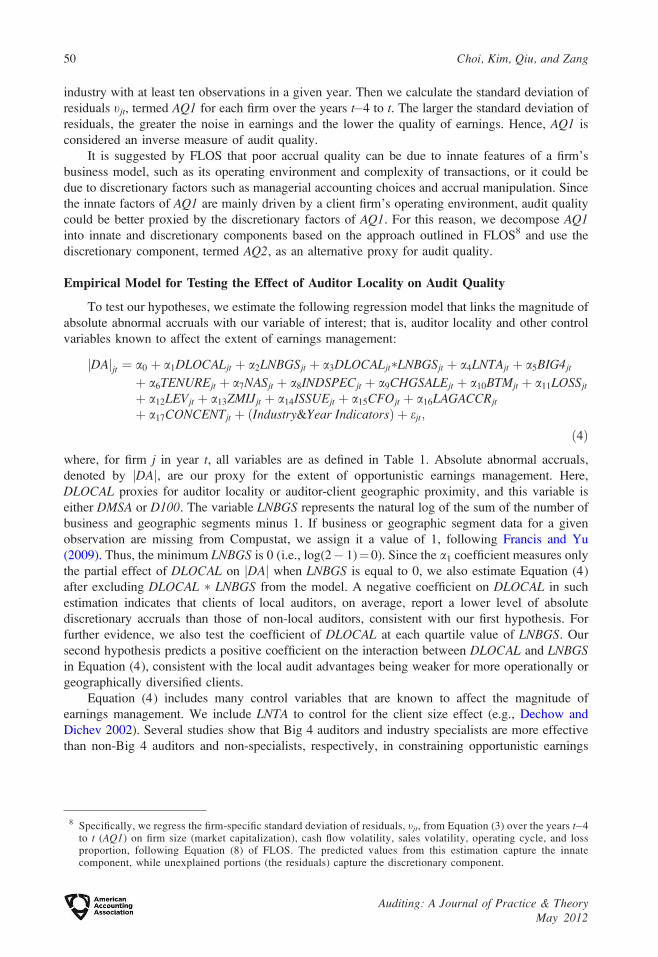
Empirical Model for Testing the Effect of Auditor Locality on Audit Quality

To test our hypotheses, we estimate the following regression model that links the magnitude of

absolute abnormal accruals with our variable of interest; that is, auditor locality and other control

variables known to affect the extent of earnings management:

jDAjjt ¼ a0 þ a1DLOCALjt þ a2LNBGSjt þ a3DLOCALjt�LNBGSjt þ a4LNTAjt þ a5BIG4jt

þ a6TENUREjt þ a7NASjt þ a8INDSPECjt þ a9CHGSALEjt þ a10BTMjt þ a11LOSSjt

þ a12LEVjt þ a13ZMIJjt þ a14ISSUEjt þ a15CFOjt þ a16LAGACCRjt

þ a17CONCENTjt þ ðIndustry&Year IndicatorsÞ þ ejt;

ð4Þ

where, for firm j in year t, all variables are as defined in Table 1. Absolute abnormal accruals,

denoted by jDAj, are our proxy for the extent of opportunistic earnings management. Here,

DLOCAL proxies for auditor locality or auditor-client geographic proximity, and this variable is

either DMSA or D100. The variable LNBGS represents the natural log of the sum of the number of

business and geographic segments minus 1. If business or geographic segment data for a given

observation are missing from Compustat, we assign it a value of 1, following Francis and Yu

(2009). Thus, the minimum LNBGS is 0 (i.e., log(2� 1)¼0). Since the a1 coefficient measures only

the partial effect of DLOCAL on jDAj when LNBGS is equal to 0, we also estimate Equation (4)

after excluding DLOCAL � LNBGS from the model. A negative coefficient on DLOCAL in such

estimation indicates that clients of local auditors, on average, report a lower level of absolute

discretionary accruals than those of non-local auditors, consistent with our first hypothesis. For

further evidence, we also test the coefficient of DLOCAL at each quartile value of LNBGS. Our

second hypothesis predicts a positive coefficient on the interaction between DLOCAL and LNBGSin Equation (4), consistent with the local audit advantages being weaker for more operationally or

geographically diversified clients.

Equation (4) includes many control variables that are known to affect the magnitude of

earnings management. We include LNTA to control for the client size effect (e.g., Dechow and

Dichev 2002). Several studies show that Big 4 auditors and industry specialists are more effective

than non-Big 4 auditors and non-specialists, respectively, in constraining opportunistic earnings

8 Specifically, we regress the firm-specific standard deviation of residuals, tjt, from Equation (3) over the years t�4to t (AQ1) on firm size (market capitalization), cash flow volatility, sales volatility, operating cycle, and lossproportion, following Equation (8) of FLOS. The predicted values from this estimation capture the innatecomponent, while unexplained portions (the residuals) capture the discretionary component.



TABLE 1

Variable Definitions and Measurements

jDAj ¼ Absolute value of discretionary (abnormal) accruals. The current study uses two

proxies: DA1 and DA2, where DA1 is abnormal accruals as measured by Ball and

Shivakumar’s (2006) method; DA2 is performance-matched abnormal accruals as

measured by Kothari et al.’s (2005) method.

AQ ¼ Accrual quality, where AQ1 is the accrual quality as measured by Dechow and

Dichev’s (2002) method; AQ2 comprises discretionary components of accrual quality

as measured by Francis et al.’s (2005a) method.

DLOCAL ¼ Indicator variable for auditor location. We use two proxies, DMSA and D100, where

DMSA is 1 if the audit office and client firm’s headquarters are located in the same

MSA, and 0 otherwise; D100 is 1 if the distance between the audit office and the

client firm’s headquarters is less than 100 kilometers, or if the audit office and the

client firm’s headquarters are located in the same MSA, and 0 otherwise.

LNBGS ¼ Natural log of the sum of the number of business and geographic segments minus 1. If

business or geographic segment data are missing for a given observation from

Compustat, we assign it a value of 1. Thus, the minimum value of LNBGS is 0; i.e.,

log(2 � 1) ¼ 0.

LNTA ¼ Natural log of total assets in thousands of dollars.

BIG4 ¼ 1 if the auditor is one of the Big 4 firms, and 0 otherwise.

TENURE ¼ Auditor tenure, measured as the natural log of the number of years the incumbent

auditor has served the client firm.

NAS ¼ Relative importance of nonaudit services, measured as the ratio of the natural log of

nonaudit fees over the natural log of total fees.

INDSPEC ¼ An indicator variable for auditor industry expertise that equals 1 if the audit firm is the

industry leader for the audit year in the audit market of the MSA where the auditor is

located, and 0 otherwise. We calculate each audit firm’s industry market share of

audit fees for an MSA as the proportion of audit fees earned by each firm in the total

audit fees earned by all audit firms in the MSA that serve the same industry. Each

industry is defined based on two-digit SIC codes.

CHGSALE ¼ Change in sales deflated by lagged total assets.

BTM ¼ Book-to-market ratio, winsorized at 0 and 4.

LOSS ¼ 1 if the firm reports a loss for the year, and 0 otherwise.

LEV ¼ Leverage, measured as total liabilities divided by total assets.

ZMIJ ¼ Zmijewski’s (1984) financial distress score, winsorized at 5 and �5.

ISSUE ¼ 1 if the sum of debt or equity issued during the past three years is more than 5 percent

of the total assets, and 0 otherwise.

CFO ¼ Operating cash flows, taken from the cash flow statement, deflated by lagged total

assets.

LAGACCR ¼ One-year lagged total accruals. Accruals are defined as income before extraordinary

items minus operating cash flows from the statement of cash flow deflated by lagged

total assets.

CONCENT ¼ A measure of auditor concentration by each MSA, measured by the Herfindahl index of

the number of clients for each audit office.

OPCYCLE ¼ Length of the operating cycle; the log of the sum of a firm’s days accounts receivable

and days inventory.

STD_CFO ¼ Cash flow variability; the standard deviation of a firm’s rolling five-year cash flows

from operations, scaled by averaged total assets.

STD_SALES ¼ Sales variability; the standard deviation of a firm’s rolling five-year sales revenues,

scaled by averaged total assets.

(continued on next page)



management (Becker et al. 1998; Krishnan 2003).9 We include BIG4 and INDSPEC to control for

the effect of auditor brand name at the national level and industry expertise at the MSA level,

respectively. We include TENURE because Johnson et al. (2002) and Myers et al. (2003) provide

evidence that clients of longer-tenure auditors report lower abnormal accruals. We include NAS to

control for the effect of nonaudit fees on audit quality (Ashbaugh et al. 2003; Chung and Kallapur

2003; Frankel et al. 2002). The variables BTM and CHGSALE are included to control for firm

growth, while LOSS is included to control for potential differences in earnings management

between loss and profit firms. We also include ZMIJ and ISSUE to control for the effects of

financial distress (Reynolds and Francis 2000) and financing transactions (Teoh et al. 1998) on

earnings management, respectively. The variable LEV is included because highly levered firms may

have greater incentives for earnings management due to their concerns of debt covenant violations

(Becker et al. 1998; DeFond and Jiambalvo 1994). We include CFO to control for the potential

correlation between accruals and cash flows (Kothari et al. 2005). As in Ashbaugh et al. (2003) and

Kim et al. (2003), we include LAGACCR to control for the reversal of accruals over time. The

variable CONCENT is included to control for the effect of auditor concentration on our results

(Kedia and Rajgopal 2011; Kallapur et al. 2010).10 Finally, we include industry and year indicators

to control for possible variations in accounting standards and regulations across industries and over

years. Each industry is defined based on two-digit SIC codes.

Next, when AQ is used as the proxy for audit quality, we estimate the following regression

model:

AQjt ¼ b0 þ b1DLOCALjt þ b2LNBGSjt þ b3DLOCALjt�LNBGSjt þ b4LNTAjt þ b5BIG4jt

þ b6OPCYCLEjt þ b7STD CFOjt þ b8STD SALEjt þ b9NASjt þ b10INDSPECjt

þ b11ZMIJjt þ b12CFOjt þ ðIndustry&Year IndicatorsÞ þ ejt;

ð5Þ

where, for firm j in year t, all variables are as defined in Table 1. We add OPCYCLE, STD_CFO,

TABLE 1 (continued)

LNSALES ¼ Natural log of sales.

NEGEAR ¼ Inventory and receivables divided by total assets.

GCM ¼ 1 if the firm receives a going-concern audit opinion in the current year, and 0

otherwise.

CAIN ¼ Capital intensity measured by long-term assets divided by total assets.

NBIG ¼ Number of Big 4 audit offices in the MSA.

WAGE ¼ Mean hourly auditor wage in the client firm’s MSA, from Occupational Employment

Statistics, Bureau of Labor Statistics, U.S. Department of Labor.

ANA ¼ Natural log of 1 plus the number of analysts following the firm.

INST ¼ Natural log of 1 plus the percentage of institutional shareholdings.

9 In contrast, Louis (2005) suggests that non-Big 4 auditors may provide better-quality audit service to smallclients. We also add an indicator variable for the middle four second-tier auditors in both Equations (4) and (5).Prior studies by Hogan and Martin (2009) and Boone et al. (2010) suggest that second-tier auditors behavedifferently from top-tier auditors and other small auditors. Because we obtain qualitatively similar results afterincluding this indicator variable, we do not tabulate them for simplicity. Based on p � 10 percent (two-tailed) asa cutoff for the significance level, this paper defines ‘‘qualitatively similar’’ to mean that in Equations (4) and (5),(1) the coefficient on DLOCAL is negative and significant, and (2) the coefficient of DLOCAL � LNBGS ispositive and significant.

10 When we measure CONCENT using audit fees rather than the number of clients, we obtain qualitatively similarresults.



and STD_SALE to Equation (5) because Dechow and Dichev (2002) argue that a longer operating

cycle and greater operating volatility are associated with higher accrual estimation errors. We also

add in Equation (5) several other control variables (NAS, INDSPEC, ZMIJ, and CFO) included in

Equation (4) that are deemed to be associated with accrual quality.11 Our variables of interest,

DLOCAL and DLOCAL � LNBGS, are the same as in Equation (4).

SAMPLE AND DESCRIPTIVE STATISTICS

Sample

The initial list of our sample consists of all firms included in the Audit Analytics database for the

four-year period 2002–2005. We extract data on the state/city locations of auditors’ practicing offices

and client firms’ headquarters from the Audit Analytics database.12 Since an MSA consists of one or

more counties, we match their city-level locations to the county codes of Federal Information

Processing Standards using the U.S. Census Bureau’s 2000 Places file, and identify whether the

practicing office of the auditor and the client’s headquarters are located in the same MSA. Following

Francis et al. (2005b), we delete observations if auditors or clients are not located in one of the 280

MSAs defined in the U.S. census of 2000.13 Next, we obtain the latitude and longitude data for the

cities of the practicing offices of auditors and the headquarters of client firms, using the U.S. Census

Bureau’s Gazetteer 2001 City-State file. With these data, we compute the actual geographic distances

between the (centers of ) two cities where auditor offices and client headquarters are located.14

We also obtain nonaudit fees data from the Audit Analytics database. We retrieve all other

financial data from the Compustat Industrial annual file. We exclude financial institutions and utility

firms with SIC codes in the ranges 6000–6999 and 4900–4999, respectively. After applying the

above selection procedures and data requirements, we obtain 12,439 firm-year observations located

in 192 MSAs. These observations are audited by auditors from 767 unique audit practice offices

located in 110 MSAs. The sample size for the tests using Equation (5) decreases by almost a half, to

6,640, due to further data requirements.

Appendix A provides information on the locations of clients and auditors in our full sample.

Column (1) of Panel A of Appendix A reports the number of clients (firm-year observations) in

each MSA where more than 100 clients are located. Column (2) reports the number of local audits

performed by audit offices located in the same MSA as their clients. Column (3) shows the average

percentage of local audits in each MSA. The percentage varies across MSAs, suggesting that the

choice of non-local auditors is not concentrated in certain MSAs. We find that about 80 percent of

11 Alternatively, we repeat the tests after including in Equation (5) all the control variables used in Equation (4).Untabulated results for the variables of interest are qualitatively identical to those tabulated in this study, and allstatistical inferences remain unchanged.

12 While Compustat reports only the current state/county codes of firms’ headquarters, Audit Analytics updates theinformation on the state/city locations of client headquarters on an annual basis. Thus, we use the AuditAnalytics database to identify client firm locations.

13 In our initial sample, we find 485 observations for which auditor or client headquarters are not located in any ofthe MSAs. Applying this selection criterion, we remove all firms that are located in a remote area in which localauditors hardly exist. As a sensitivity check, we repeat our analyses after including these observations andtreating them as (1) DMSA¼ 1, (2) DMSA¼ 0, or (3) DMSA¼ 1 or 0, following the definition of D100. We find,however, that the inclusion of these observations in our sample does not alter our statistical inferences for any ofthe three cases.

14 When the auditor’s practicing office and the client’s headquarters are in the same city, the distance is calculatedas zero. It is possible that the effect of auditor locality is stronger when the two offices are located within ashorter distance within the city, but data unavailability limits such analyses (i.e., no street-level addresses forauditors’ offices are available in the Audit Analytics database). For more details on distance computation, seeCoval and Moskowitz (1999).



audits are carried out by auditors located in the same MSA, and about 83 percent are by auditors

located within 100 kilometers. Accordingly, only about 3 percent of firms are audited by auditors

located within 100 kilometers, but not in the same MSA. There are not many cases (only 62

observations, reported in the bottom row of Panel A of Appendix A) where auditors are located in

the same MSA as their clients, but farther than 100 kilometers away from the clients’ headquarters.

Panel B reports the number of observations by the distance between the audit office and client

headquarters when they are not located in the same MSA. It is clear from Panel B that some

auditors are located nearby, even though they are not in the same MSA as their client firms.

Panel C of Appendix A provides more detailed auditor location information for 1,691 clients

located in the New York-Northern New Jersey-Long Island MSA.15 It shows that about 15 percent

of the clients in the MSA hire auditors from other MSAs, and about 13 percent of the clients hire

auditors located farther than 100 kilometers from their headquarters. It is noteworthy that some

clients in the New York-Northern New Jersey-Long Island MSA hire auditors located far away,

such as from the San Francisco-Oakland-San Jose MSA (4,120 kilometers away, on average), the

Los Angeles-Riverside-Orange County MSA (3,949 kilometers away), and the Denver-Boulder-

Greeley MSA (2,644 kilometers away).16 In contrast, some auditors come from nearby MSAs, such

as the Hartford MSA (69 kilometers away) and the Philadelphia-Wilmington-Atlantic City MSA

(73 kilometers away). These auditors are likely to share the characteristics of the local auditors to

the client firms even though they are not located in the same MSA. This is why we define D100 as a

combined variable of the distance-based and MSA-based measures and use it (in addition to DMSA,

which is an MSA-based measure) to proxy for local audits.

Descriptive Statistics and Univariate Tests

Panels A and B of Table 2 present the descriptive statistics for our two discretionary accrual

measures, jDA1j and jDA2j, and two accrual quality measures, AQ1 and AQ2, separately, for the local

auditor sample (DMSA¼ 1 or D100¼ 1) and the non-local auditor sample (DMSA¼ 0 or D100¼ 0),

along with univariate test results for differences in the mean and median between the two samples. As

shown in Panels A and B of Table 2, both jDA1j and jDA2j are significantly lower for the clients of

local auditors than for those of non-local auditors. For example, the mean (median) value of jDA1j is0.0846 (0.0473) for the clients of local auditors located in the same MSA, and 0.1046 (0.0570) for

those of non-local auditors located in a different MSA. The differences are significant at the 1 percent

level (t¼�7.90). We also find similar differences for the accrual quality measures.

Panel C of Table 2 reports the descriptive statistics for all other variables included in our main

regressions. The sample firms have 3.5 business or geographic segments, on average (LNBGS ¼0.9170). The average client size (LNTA) is 12.2340, which is equivalent to about $200 million of

total assets. About 77 percent of clients are audited by one of the Big 4 auditors (BIG4), and the

average logged auditor tenure (TENURE) is 1.8410, which is interpreted as about six years of

auditor tenure. On average, nonaudit service fees (NAS) are about 67 percent of total fees, and about

15 We choose the New York-Northern New Jersey-Long Island MSA, for example, because the number of clientfirms located in this MSA is the largest of our sample.

16 To check if there exist any special reasons to hire long-distance, non-local auditors, we choose the state ofCalifornia (where the state-by-state sample size is the largest), and identify clients that hire auditors located atleast 300 miles away from client headquarters. We find that 50 client firms (101 observations) belong to thiscategory. For these firms, we search for 10-Ks from the EDGAR database to see if these firms have specialconnections with the states in which their auditors are located. We find that out of 50 client firms, 16 have othermajor offices or plants (except for headquarters) in the states where their auditors are located, and four movedtheir headquarters to California from different states, but continued to hire their previous auditors. However, wehave been unable to find any compelling evidence that the remaining 30 clients have any special connections tothe states in which their auditors are located.



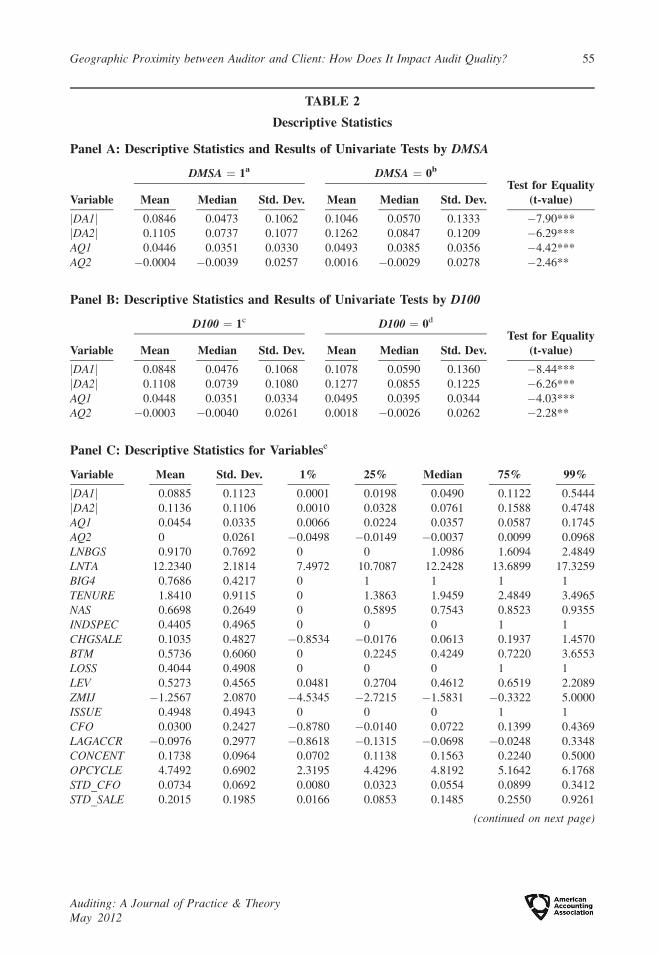
TABLE 2

Descriptive Statistics

Panel A: Descriptive Statistics and Results of Univariate Tests by DMSA

Variable

DMSA ¼ 1a DMSA ¼ 0b

Mean Median Std. Dev. Mean Median Std. Dev.Test for Equality

(t-value)

jDA1j 0.0846 0.0473 0.1062 0.1046 0.0570 0.1333 �7.90***

jDA2j 0.1105 0.0737 0.1077 0.1262 0.0847 0.1209 �6.29***

AQ1 0.0446 0.0351 0.0330 0.0493 0.0385 0.0356 �4.42***

AQ2 �0.0004 �0.0039 0.0257 0.0016 �0.0029 0.0278 �2.46**

Panel B: Descriptive Statistics and Results of Univariate Tests by D100

Variable

D100 ¼ 1c D100 ¼ 0d

Mean Median Std. Dev. Mean Median Std. Dev.Test for Equality

(t-value)

jDA1j 0.0848 0.0476 0.1068 0.1078 0.0590 0.1360 �8.44***

jDA2j 0.1108 0.0739 0.1080 0.1277 0.0855 0.1225 �6.26***

AQ1 0.0448 0.0351 0.0334 0.0495 0.0395 0.0344 �4.03***

AQ2 �0.0003 �0.0040 0.0261 0.0018 �0.0026 0.0262 �2.28**

Panel C: Descriptive Statistics for Variablese

Variable Mean Std. Dev. 1% 25% Median 75% 99%

jDA1j 0.0885 0.1123 0.0001 0.0198 0.0490 0.1122 0.5444

jDA2j 0.1136 0.1106 0.0010 0.0328 0.0761 0.1588 0.4748

AQ1 0.0454 0.0335 0.0066 0.0224 0.0357 0.0587 0.1745

AQ2 0 0.0261 �0.0498 �0.0149 �0.0037 0.0099 0.0968

LNBGS 0.9170 0.7692 0 0 1.0986 1.6094 2.4849

LNTA 12.2340 2.1814 7.4972 10.7087 12.2428 13.6899 17.3259

BIG4 0.7686 0.4217 0 1 1 1 1

TENURE 1.8410 0.9115 0 1.3863 1.9459 2.4849 3.4965

NAS 0.6698 0.2649 0 0.5895 0.7543 0.8523 0.9355

INDSPEC 0.4405 0.4965 0 0 0 1 1

CHGSALE 0.1035 0.4827 �0.8534 �0.0176 0.0613 0.1937 1.4570

BTM 0.5736 0.6060 0 0.2245 0.4249 0.7220 3.6553

LOSS 0.4044 0.4908 0 0 0 1 1

LEV 0.5273 0.4565 0.0481 0.2704 0.4612 0.6519 2.2089

ZMIJ �1.2567 2.0870 �4.5345 �2.7215 �1.5831 �0.3322 5.0000

ISSUE 0.4948 0.4943 0 0 0 1 1

CFO 0.0300 0.2427 �0.8780 �0.0140 0.0722 0.1399 0.4369

LAGACCR �0.0976 0.2977 �0.8618 �0.1315 �0.0698 �0.0248 0.3348

CONCENT 0.1738 0.0964 0.0702 0.1138 0.1563 0.2240 0.5000

OPCYCLE 4.7492 0.6902 2.3195 4.4296 4.8192 5.1642 6.1768

STD_CFO 0.0734 0.0692 0.0080 0.0323 0.0554 0.0899 0.3412

STD_SALE 0.2015 0.1985 0.0166 0.0853 0.1485 0.2550 0.9261




44 percent of clients hire industry specialists (INDSPEC). The distributions of the other variables

are also shown in Panel B of Table 2. When the descriptive statistics in Panel B are compared with

other studies on audit office-level analyses, we find that ours are quite comparable to those of Choi

et al. (2010) and Francis and Yu (2009).

Panels A and B of Table 3 present the Pearson correlation matrix for all the variables included

in Equation (4). The two abnormal accrual measures, jDA1j and jDA2j, are highly correlated with

the correlation coefficient of 0.445 (p , 0.01). The auditor locality indicators, DMSA and D100, are

negatively correlated with jDA1j and jDA2j (p , 0.01 for both). Both jDA1j and jDA2j are

significantly correlated with many control variables, supporting their inclusion as control variables.

Finally, we note that the correlations between the control variables are mostly not very high, except

for those between BIG4 and LNTA (0.547) and between NAS and LNTA (0.436). This finding

suggests that multicollinearity is unlikely to be a serious problem.

Panels C and D of Table 3 present the Pearson correlations among the variables included in

Equation (5), which can be summarized as follows. First, as expected, the two accrual quality metrics,

AQ1 and AQ2, are highly correlated with each other. Second, both accrual quality metrics are

negatively correlated with our measures of auditor locality, DMSA and D100, which is consistent with

the results of univariate tests (as reported in Panels A and B of Table 2). Third, control variables are

highly correlated with our accrual quality measures. Finally, consistent with the findings in Panels A

and B of Table 3, the correlations between our control variables are mostly not very high, except for

those between BIG4 and LNTA (0.520) and between NAS and LNTA (0.436).

EMPIRICAL RESULTS

Main Results Using Discretionary Accrual Measures

Table 4 reports the results of the regression in Equation (4). In Section A (B), jDA1j (jDA2j) is

used as the dependent variable. All reported t-statistics are on an adjusted basis, using standard

errors corrected for clustering at the firm level and heteroscedasticity. As shown in Columns (1a)

and (3a), we first estimate Equation (4) after excluding DLOCAL � LNBGS from the model. The

coefficients on DMSA and D100 are both negative and significant (�0.0046 with t ¼�1.77, and

�0.0050 with t ¼�1.73) at the 10 percent level in two-tailed tests.17 These results are consistent

with H1, that local auditors are, on average, more effective than non-local auditors in deterring

opportunistic earnings management or biased financial reporting. These results should be

interpreted cautiously, however, because the omission of DLOCAL � LNBGS can create a potential

TABLE 2 (continued)

*, **, *** Denote p-values of less than 10 percent, 5 percent, and 1 percent, with two-tailed tests, respectively.a The sample size is 9,996 for jDA1j and jDA2j, and 5,408 firm-year observations for AQ1 and AQ2.b The sample size is 2,443 for jDA1j and jDA2j, and 1,232 firm-year observations for AQ1 and AQ2.c The sample size is 10,428 for jDA1j and jDA2j, and 5,687 firm-year observations for AQ1 and AQ2.d The sample size is 2,011 for jDA1j and jDA2j, and 953 firm-year observations for AQ1 and AQ2.e The sample size is 12,439 for jDA1j, jDA2j, and 15 variables from LNBGS to CONCENT, and 6,640 firm-year

observations for AQ1, AQ2, and the other three variables from OPCYCLE to STD_SALE.

17 When jDA2j is used as the dependent variable in the model excluding DLOCAL � LNBGS, the coefficients onDMSA and D100 are�0.0037 (t¼�1.49) and�0.0028 (t¼�1.15). While the coefficient on DMSA is significant,with p ¼ 0.0685 in a one-tailed test, the coefficient on D100 is insignificant.



TABLE 3

Correlation Matrix

Panel A: Pearson Correlations between Discretionary Accruals, Auditor Locality, andControl Variables from jDA1j to NAS

jDA1j jDA2j DMSA D100 LN-BGS LNTA BIG4 TENURE NAS

jDA2j 0.445

(,0.01)

DMSA �0.071 �0.056

(,0.01) (,0.01)

D100 �0.076 �0.056 0.888

(,0.01) (,0.01) (,0.01)

LNBGS �0.141 �0.131 0.061 0.068

(,0.01) (,0.01) (,0.01) (,0.01)

LNTA �0.319 �0.305 0.127 0.122 0.362

(,0.01) (,0.01) (,0.01) (,0.01) (,0.01)

BIG4 �0.212 �0.195 0.163 0.173 0.197 0.547

(,0.01) (,0.01) (,0.01) (,0.01) (,0.01) (,0.01)

TENURE �0.098 �0.077 0.045 0.042 0.116 0.253 0.287

(,0.01) (,0.01) (,0.01) (,0.01) (,0.01) (,0.01) (,0.01)

NAS �0.144 �0.148 0.097 0.099 0.222 0.436 0.357 0.224

(,0.01) (,0.01) (,0.01) (,0.01) (,0.01) (,0.01) (,0.01) (,0.01)

INDSPEC �0.118 �0.106 �0.020 �0.002 0.092 0.318 0.304 0.132 0.157

(,0.01) (,0.01) (0.02) (0.798) (,0.01) (,0.01) (,0.01) (,0.01) (,0.01)

CHGSALE 0.028 0.002 0.017 0.013 0.001 0.064 0.012 0.010 0.026

(,0.01) (0.870) (0.06) (0.162) (0.992) (,0.01) (0.19) (0.27) (,0.01)

BTM �0.083 0.138 �0.035 �0.018 �0.009 �0.065 �0.042 �0.034 �0.021

(,0.01) (,0.01) (,0.01) (0.042) (0.295) (,0.01) (,0.01) (,0.01) (0.02)

LOSS 0.256 0.198 �0.063 �0.069 �0.135 �0.360 �0.171 �0.127 �0.168

(,0.01) (,0.01) (,0.01) (,0.01) (,0.01) (,0.01) (,0.01) (,0.01) (,0.01)

LEV 0.151 0.079 �0.071 �0.083 �0.024 �0.068 �0.131 �0.038 �0.061

(,0.01) (,0.01) (,0.01) (,0.01) (,0.01) (,0.01) (,0.01) (,0.01) (,0.01)

ZMIJ 0.238 �0.138 �0.090 �0.104 �0.076 �0.142 �0.147 �0.078 �0.098

,(0.01) (,0.01) (,0.01) (,0.01) (,0.01) (,0.01) (,0.01) (,0.01) (,0.01)

ISSUE 0.081 0.053 �0.049 �0.053 �0.056 �0.015 �0.033 �0.030 �0.031

(,0.01) (,0.01) (,0.01) (,0.01) (,0.01) (0.09) (,0.01) (,0.01) (,0.01)

CFO �0.273 �0.072 0.061 0.068 0.163 0.369 0.179 0.083 0.191

(,0.01) (,0.01) (,0.01) (,0.01) (,0.01) (,0.01) (,0.01) (,0.01) (,0.01)

LAGACCR �0.122 �0.216 0.034 0.035 0.053 0.101 0.070 0.043 0.062

(,0.01) (,0.01) (,0.01) (,0.01) (,0.01) (,0.01) (,0.01) (,0.01) (,0.01)

CONSERV �0.054 �0.082 �0.031 �0.014 0.026 0.046 0.078 0.040 0.085

(,0.01) (,0.01) (,0.01) (0.117) (,0.01) (,0.01) (,0.01) (,0.01) (,0.01)

Panel B: Pearson Correlations between Discretionary Accruals, Auditor Locality, andControl Variables from INDSPEC to LAGACCR

INDSPEC CHGSALE BTM LOSS LEV ZMIJ ISSUE CFO LAGACCR

CHGSALE 0.018

(0.05)




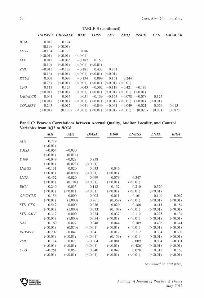
TABLE 3 (continued)

INDSPEC CHGSALE BTM LOSS LEV ZMIJ ISSUE CFO LAGACCR

BTM �0.012 �0.124

(0.19) (,0.01)

LOSS �0.134 �0.178 0.086

(,0.01) (,0.01) (,0.01)

LEV 0.012 �0.085 �0.187 0.153

(0.19) (,0.01) (,0.01) (,0.01)

ZMIJ �0.013 �0.128 �0.181 0.433 0.761

(0.16) (,0.01) (,0.01) (,0.01) (,0.01)

ISSUE 0.003 0.093 �0.134 0.099 0.151 0.244

(0.73) (,0.01) (,0.01) (,0.01) (,0.01) (,0.01)

CFO 0.113 0.124 0.043 �0.502 �0.119 �0.421 �0.189

(,0.01) (,0.01) (,0.01) (,0.01) (,0.01) (,0.01) (,0.01)

LAGACCR 0.041 0.035 0.051 �0.139 �0.163 �0.078 �0.078 0.175

(,0.01) (,0.01) (,0.01) (,0.01) (,0.01) (,0.01) (,0.01) (,0.01)

CONSERV 0.243 �0.012 0.041 �0.049 �0.041 �0.049 �0.021 0.029 0.015

(,0.01) (0.170) (,0.01) (,0.01) (,0.01) (,0.01) (0.020) (0.001) (0.087)

Panel C: Pearson Correlations between Accrual Quality, Auditor Locality, and ControlVariables from AQ1 to BIG4

AQ1 AQ2 DMSA D100 LNBGS LNTA BIG4

AQ2 0.779

(,0.01)

DMSA �0.054 �0.030

(,0.01) (0.014)

D100 �0.049 �0.028 0.858

(,0.01) (0.023) (,0.01)

LNBGS �0.131 0.020 0.033 0.046

(,0.01) (0.099) (,0.01) (,0.01)

LNTA �0.452 �0.020 0.099 0.079 0.347

(,0.01) (0.104) (,0.01) (,0.01) (,0.01)

BIG4 �0.240 �0.035 0.118 0.132 0.210 0.520

(,0.01) (,0.01) (,0.01) (,0.01) (,0.01) (,0.01)

OPCYCLE 0.156 �0.000 �0.002 0.011 0.161 �0.140 �0.062

(,0.01) (1.000) (0.861) (0.359) (,0.01) (,0.01) (,0.01)

STD_CFO 0.542 0.000 �0.026 �0.020 �0.186 �0.411 0.184

(,0.01) (1.000) (0.033) (0.108) (,0.01) (,0.01) (,0.01)

STD_SALE 0.317 0.000 �0.024 �0.037 �0.112 �0.225 �0.134

(,0.01) (1.000) (0.054) (,0.01) (,0.01) (,0.01) (,0.01)

NAS �0.169 0.022 0.048 0.044 0.189 0.436 0.341

(,0.01) (0.070) (,0.01) (,0.01) (,0.01) (,0.01) (,0.01)

INDSPEC �0.202 �0.047 �0.041 �0.017 0.112 0.334 0.308

(,0.01) (,0.01) (,0.01) (0.159) (,0.01) (,0.01) (,0.01)

ZMIJ 0.114 0.077 �0.064 �0.081 0.009 0.034 �0.031

(,0.01) (,0.01) (,0.01) (,0.01) (0.486) (,0.01) (,0.01)

CFO �0.251 0.052 0.040 0.047 0.078 0.312 0.168

(,0.01) (,0.01) (,0.01) (,0.01) (,0.01) (,0.01) (,0.01)




problem of correlated omitted variables. In what follows, we test our H1 and H2 using the results of

estimating the full model in Equation (4).

When we include DLOCAL � LNBGS in the model, the coefficients on both DMSA and D100

all remain significantly negative, as shown in Columns (2a), (4a), (1b), and (2b). Furthermore, the

interaction term between DLOCAL and LNBGS is positive and significant across all columns in

both Sections A and B of Table 4; for example, in Column (2a), the coefficient on the interaction

term is positive and significant at the 5 percent level (0.0086, with t¼ 2.45). These results support

H2, implying that the effect of local audits on audit quality is weaker for more diversified client

firms.18

To further examine the validity of H1, we investigate whether the clients of local auditors

report a lower level of discretionary accruals at different levels of firm diversification. When we set

the value of LNBGS at the 25th percentile (LNBGS¼ 0, from Panel B of Table 2), the coefficient on

DMSA and DMSA � LNBGS in Column (2a) of Table 4 is translated into �0.0119 (�0.0119 þ[0.0086 � 0] ¼�0.0119). This implies that discretionary accruals of clients of local auditors are

lower than those of clients of non-local auditors by 0.0119, when the value of LNBGS is equal to its

25th percentile value. However, when we set the value of LNBGS at the 50th (LNBGS¼ 1.0986),

75th (LNBGS ¼ 1.6094), or 99th (LNBGS ¼ 2.4849) percentile value, we fail to find significant

differences in the level of discretionary accruals between local and non-local auditors. As reported

in the bottom three rows of Table 4, the F-test result for the sum of the coefficients on DLOCAL and

TABLE 3 (continued)

Panel D: Pearson Correlations between Accrual Quality, Auditor Locality, and ControlVariables from OPCYCLE to ZMIJ

OPCYCLE STD_CFO STD_SALE NAS INDSPEC ZMIJ

STD_CFO 0.101

(,0.01)

STD_SALE �0.128 0.344

(,0.01) (,0.01)

NAS 0.001 �0.166 �0.089

(0.934) (,0.01) (,0.01)

INDSPEC �0.105 �0.149 �0.081 0.190

(,0.01) (,0.01) (,0.01) (,0.01)

ZMIJ �0.130 0.087 0.074 �0.002 0.046

(,0.01) (,0.01) (,0.01) (0.856) (,0.01)

CFO �0.192 �0.359 �0.063 0.181 0.124 �0.411

(,0.01) (,0.01) (,0.01) (,0.01) (,0.01) (,0.01)

Two-tailed p-values are presented in parentheses.

18 To examine whether local audits constrain either or both income-increasing and income-decreasing accruals, wesplit the full sample into two subsamples, with income-increasing (positive) and income-decreasing (negative)accruals (i.e., DA1 . 0 and DA1 , 0), and then estimate Equation (4) separately. Untabulated results suggestthat the coefficients on DLOCAL and DLOCAL � LNBGS are significant with predicted signs when we use thesubsample of income-increasing accruals. However, when we use the subsample of income-decreasing accruals,both coefficients are insignificant, although they have the expected signs. These results suggest thatinformational advantages associated with local audits are related to more accurate accruals in general, but theeffect is stronger for reducing income-increasing accruals. This finding is not very surprising, because auditorstend to be more concerned about their clients’ income-increasing accruals (Kim et al. 2003).



TA

BL

E4

Ass

oci

ati

on

bet

wee

nA

ud

ito

rL

oca

lity

an

dC

lien

ts’

Dis

cret

ion

ary

Acc

rua

ls

Ex

pec

ted

Sig

n

Sec

tio

nA

Usi

ngjD

A1ja

sth

eD

epen

den

tV

ari

ab

leS

ecti

on

BU

sin

gjD

A2ja

sth

eD

epen

den

tV

ari

ab

le

(1a

)D

LO

CA

L¼

DM

SA

(2a

)D

LO

CA

L¼

DM

SA

(3a

)D

LO

CA

L¼

D1

00

(4a

)D

LO

CA

L¼

D1

00

(1b

)D

LO

CA

L¼

DM

SA

(2b

)D

LO

CA

L¼

D1

00

DL

OC

AL

��

0.0

04

6�

0.0

11

9�

0.0

05

0�

0.0

12

1�

0.0

09

0�

0.0

08

3

(�1

.77

*)

(�2

.75

**

*)

(�1

.73

*)

(�2

.58

**

*)

(�2

.26

**

)(�

1.9

7*

*)

LN

BG

S?

�0

.00

53

�0

.01

21

�0

.00

53

�0

.01

24

�0

.00

96

�0

.01

02

(�3

.68

**

*)

(�3

.72

**

*)

(�3

.67

**

*)

(�3

.42

**

*)

(�2

.98

**

*)

(�2

.97

**

*)

DL

OC

AL�

LN

BG

Sþ

—0

.00

86

—0

.00

86

0.0

06

20

.00

66

(2.4

5*

*)

(2.2

4*

*)

(1.7

8*

)(1

.82

*)

LN

TA

��

0.0

10

6�

0.0

10

6�

0.0

10

6�

0.0

10

6�

0.0

10

7�

0.0

10

7

(�1

4.4

4*

**

)(�

14

.48

**

*)

(�1

4.4

6*

**

)(�

14

.49

**

*)

(�1

5.0

8*

**

)(�

15

.11

**

*)

BIG

4�

�0

.01

31

�0

.01

29

�0

.01

30

�0

.01

28

�0

.01

20

�0

.01

21

(�3

.96

**

*)

(�3

.90

**

*)

(�3

.94

**

*)

(�3

.88

**

*)

(�3

.78

**

*)

(�3

.80

**

*)

TE

NU

RE

�0

.00

03

0.0

00

20

.00

03

0.0

00

20

.00

15

0.0

01

5

(0.2

9)

(0.1

6)

(0.2

7)

(0.1

4)

(1.2

6)

(1.2

5)

NA

S?

0.0

06

40

.00

69

0.0

06

40

.00

68

�0

.00

17

�0

.00

18

(1.2

7)

(1.3

8)

(1.2

7)

(1.3

5)

(�0

.36

)(�

0.3

9)

IND

SPE

C�

0.0

00

80

.00

08

0.0

00

90

.00

08

0.0

02

70

.00

28

(0.3

8)

(0.3

6)

(0.4

1)

(0.3

6)

(1.2

4)

(1.2

7)

CH

GSA

LE

þ0

.02

00

0.0

20

10

.02

00

0.0

20

00

.00

85

0.0

08

5

(4.1

1*

**

)(4

.13

**

*)

(4.1

0*

**

)(4

.10

**

*)

(2.6

0*

**

)(2

.58

**

*)

BT

M�

�0

.01

12

�0

.01

12

�0

.01

11

�0

.01

11

�0

.01

17

�0

.01

17

(�5

.32

**

*)

(�5

.33

**

*)

(�5

.30

**

*)

(�5

.31

**

*)

(�5

.90

**

*)

(�5

.87

**

*)

LO

SSþ

0.0

15

50

.01

56

0.0

15

50

.01

55

0.0

12

10

.01

20

(5.5

9*

**

)(5

.62

**

*)

(5.5

8*

**

)(5

.61

**

*)

(4.7

0*

**

)(4

.68

**

*)

LE

Vþ

0.0

06

80

.00

67

0.0

06

80

.00

67

0.0

06

30

.00

63

(0.8

7)

(0.8

6)

(0.8

7)

(0.8

6)

(1.3

1)

(1.3

1)

(con

tinu

edo

nn

ext

pa

ge)



TA

BL

E4

(co

nti

nu

ed)

Ex

pec

ted

Sig

n

Sec

tio

nA

Usi

ngjD

A1ja

sth

eD

epen

den

tV

ari

ab

leS

ecti

on

BU

sin

gjD

A2ja

sth

eD

epen

den

tV

ari

ab

le

(1a

)D

LO

CA

L¼

DM

SA

(2a

)D

LO

CA

L¼

DM

SA

(3a

)D

LO

CA

L¼

D1

00

(4a

)D

LO

CA

L¼

D1

00

(1b

)D

LO

CA

L¼

DM

SA

(2b

)D

LO

CA

L¼

D1

00

ZM

IJþ

0.0

05

00

.00

51

0.0

05

00

.00

51

0.0

00

70

.00

07

(3.0

4*

**

)(3

.05

**

*)

(3.0

4*

**

)(3

.05

**

*)

(0.5

9)

(0.6

0)

ISSU

Eþ

0.0

00

20

.00

01

0.0

00

10

.00

01

0.0

00

80

.00

08

(0.0

8)

(0.0

6)

(0.0

2)

(0.0

7)

(0.3

9)

(0.4

1)

CF

O�

�0

.04

20

�0

.04

17

�0

.04

19

�0

.04

17

�0

.03

02

�0

.03

01

(�3

.41

**

*)

(�3

.39

**

*)

(�3

.41

**

*)

(�3

.39

**

*)

(�3

.64

**

*)

(�3

.64

**

*)

LA

GA

CC

R�

�0

.01

62

�0

.01

62

�0

.01

62

�0

.01

62

�0

.00

77

�0

.00

78

(�2

.53

**

)(�

2.5

3*

*)

(�2

.53

**

)(�

2.5

3*

*)

(�1

.87

*)

(�1

.88

*)

CO

NC

EN

T�

�0

.02

47

�0

.02

42

�0

.02

45

�0

.02

38

�0

.01

95

�0

.01

90

(�2

.55

**

)(�

2.5

2*

*)

(�2

.53

**

)(�

2.4

7*

*)

(�2

.02

**

)(�

1.9

8*

*)

Inte

rcep

t?

0.2

48

20

.25

40

0.2

48

80

.25

45

0.2

74

50

.27

45

(21

.61

**

*)

(20

.90

**

*)

(21

.55

**

*)

(20

.72

**

*)

(26

.69

**

*)

(26

.39

**

*)

Ind

.an

dY

ear

Ind

icat

ors

Incl

ud

edIn

clu

ded

Incl

ud

edIn

clu

ded

Incl

ud

edIn

clu

ded

n1

2,4

39

12

,43

91

2,4

39

12

,43

91

2,4

39

12

,43

9

R2

0.1

88

60

.18

91

0.1

88

60

.18

91

0.1

37

10

.13

71

Tes

tfo

r:

[a1þ

(a3�

1.0

98

6)]¼

0—

F¼

0.8

8—

F¼

0.8

0F¼

0.6

6F¼

0.1

3

Tes

tfo

r:

[a1þ

(a3�

1.6

09

4)]¼

0—

F¼

0.3

4—

F¼

0.2

3F¼

0.0

8F¼

0.4

2

Tes

tfo

r:

[a1þ

(a3�

2.4

84

9)]¼

0—

F¼

2.7

7—

F¼

2.2

5F¼

1.1

8F¼

1.7

7

*,

**,

***

Den

ote

p-v

alues

of

less

than

10

per

cent,

5per

cent,

and

1per

cent,

resp

ecti

vel

y,

wit

hF

-tes

tsan

dtw

o-t

aile

dt-

test

s.T

his

table

report

sth

ere

sult

sof

the

regre

ssio

nin

Equat

ion

(4).

All

var

iable

sar

eas

defi

ned

inT

able

1.

All

report

edt-

stat

isti

csin

par

enth

eses

are

on

anad

just

edbas

is,

usi

ng

stan

dar

der

rors

corr

ecte

dfo

rcl

ust

erin

gat

the

firm

level

and

het

erosc

edas

tici

ty.



DLOCAL � LNBGS times the 50th, 75th, or 99th percentile value of LNBGS is not significant at the

10 percent level. The results using the estimated coefficients in other columns are qualitatively

identical. These results suggest that local auditors perform higher-quality audit services than non-

local auditors, but only for relatively less diversified clients.19

To examine the economic significance of our results, we translate the estimated coefficients of

the variables of interest into the magnitude of absolute discretionary accruals as a percentage of

lagged total assets, and calculate the percentage difference between local and non-local audits using

the estimated coefficients reported in Column (2a) of Table 4. The estimated coefficient on DMSA,

�0.0119, and that on DMSA � LNBGS, 0.0086, mean that, on average, the clients of local auditors

exhibit an approximately 4 percent lower level of absolute discretionary accruals than those of non-

local auditors when we set all the other variables to their respective mean values.20 For relatively

more diversified firms (LNBGS¼ 1.6094, which is the 75th percentile value of the variable), local

audits yield a lower level of absolute discretionary accruals by about 3 percent, whereas for less

diversified firms (LNBGS¼ 0, which is the 25th percentile value), local audits yield lower absolute

discretionary accruals by about 12 percent compared with those of non-local audits. The 9 percent

difference between the 25th and 75th percentiles suggests that the effect of local audits varies

substantially with the level of firm diversification.

The coefficients on the control variables are, overall, in line with the evidence reported in prior

earnings management research. The coefficient on LNBGS is negative and significant, suggesting

that diversified firms with relatively stable operations have higher earnings quality. The coefficient

on LNTA is highly significant, with a negative sign across all four columns, suggesting that large

client firms tend to engage in earnings management to a lesser extent than small client firms

(Dechow and Dichev 2002). The coefficient on BIG4 is significantly negative in all specifications,

suggesting that Big 4 auditors are more effective than non-Big 4 auditors in constraining aggressive

earnings management. The coefficient on BTM (CHGSALE) is significantly negative (positive),

which suggests that high-growth firms manage earnings more aggressively. The coefficients on

LOSS and ZMIJ are significant, with an expected positive sign in most cases, suggesting that client

firms in financial distress are more likely to engage in earnings management. Consistent with

evidence reported in previous research (e.g., Ashbaugh et al. 2003; Kim et al. 2003), the coefficients

on CFO and LAGACCR have a negative sign. Finally, consistent with the findings in Kallapur et al.

(2010), the auditor concentration measure is negatively associated with the magnitude of absolute

discretionary accruals.

As robustness checks, we reestimate Equation (4) using the performance-unadjusted abnormal

accruals as the dependent variable—that is, using the modified Jones (1991) model in Equation (2),

as specified in Dechow et al. (1995). We also run the median regression and year-by-year

regressions after excluding year indicators. We also repeat the tests using various subsamples.

19 To further explore this issue, we form four subsamples based on the number of segments (i.e., firms with twosegments [one business segment and one geographic segment], three segments, four or five segments, and six ormore segments). We then estimate Equation (4), after excluding LNBGS and DLOCAL � LNBGS, for each of foursubsamples. When DMSA is used as DLOCAL and the dependent variable is jDA1j, the coefficient on DMSA isequal to�0.0123 (t¼�2.56) for the subsample of firms with two segments (4,272 observations). However, thecoefficient is not significant for all other subsamples. For example, the coefficient is�0.0004 (t¼�0.10) for thesubsample of firms with six or more segments (3,321 observations). When we perform additional analyses forfirms with seven or more segments, eight or more segments, and nine or more segments, the results show that thecoefficient on DMSA is insignificant, with a negative sign for each of these subsamples.

20 The average magnitude of absolute discretionary accruals as a percentage of lagged total assets estimated fromthe coefficients reported in Column (2a) is 0.1039 for the clients of non-local auditors and 0.0999 for the clientsof local auditors when we set all the other variables at their respective mean values.



Though not tabulated, the results from these robustness checks are, overall, qualitatively similar to

those reported in Table 4.21

Main Results Using Accrual Quality Measures

We further examine whether local audits are related to the accrual quality of client firms. As

explained earlier, we use both the accrual quality measure (AQ1) developed by Dechow and Dichev

(2002) and modified by McNichols (2002) and its discretionary component (AQ2), estimated based

on the approach outlined in FLOS as proxies for audit quality. We then estimate the regression

model in Equation (5). Table 5 reports the regression results using the reduced sample of 6,640

firm-year observations.

In Table 5, the coefficient on DLOCAL is negative and significant across all four columns.22 It

also shows that the coefficients on DLOCAL � LNBGS are positive and significant in all columns.

These results suggest that while auditor locality is associated with less noise in client accruals (i.e.,

greater accrual quality) in general, the association is weaker for clients with a more diversified

business structure. These findings lend further support to the results reported in Table 4. The

estimated coefficients of the control variables in Table 5 are generally consistent with those reported

in Table 4, with the notable exception that the coefficient on CFO is positively (negatively)

significant in Table 5 (Table 4).

In addition, we use the absolute values of residuals from Equation (5) to proxy for accrual

quality, as suggested by Dechow and Dichev (2002) and used by Srinidhi and Gul (2007), in

untabulated analyses. Similar to the tabulated results, we find that the variables of interest are all

significant. Overall, the results using our accrual quality measures, AQ1 and AQ2, also support our H1

and H2. Although not separately tabulated, we conduct a variety of sensitivity analyses and find that

our results are robust to different regression methods and alternative measures of our test variables.23

21 For example, for the regressions using the performance-unadjusted abnormal accruals and the median regression,the coefficients on DMSA for the regression in Column (2a) of Table 4 are�0.0188 (t¼�3.65) and�0.0091 (t¼�4.80), respectively, and those on DMSA � LNBGS are 0.0127 (t¼ 3.31) and 0.0072 (t¼ 4.41), respectively. Inyear-by-year regressions, all four yearly regressions yield negative (positive) coefficients on DMSA (DMSA �LNBGS), and two (three) of them are significant at least at the 10 percent level. The average of the yearlycoefficients on DMSA (DMSA � LNBGS) is �0.0123 (0.0087) and the corresponding Fama-MacBeth-style t-statistic is 2.79 (2.46). We also perform several additional tests using various subsamples. First, we restrict oursample to the largest 100 MSAs in terms of population. Second, we use the median size of MSAs to classify largeand small MSAs, and repeat the analyses with both subsamples. Third, we divide the full sample intoobservations from the six largest MSAs and from the other MSAs, and repeat the analyses with both subsamples.Fourth, we delete observations with auditors coming from cities located farther than 500 (1,000) kilometers awayand repeat the analyses. In sum, we find evidence consistent with the predictions of both H1 and H2 in all ofthese analyses. The coefficients on both DLOCAL and DLOCAL � LNBGS remain significant across almost allcases; the only exception is that we fail to find a significant coefficient on DLOCAL when we use observationsfrom the six largest MSAs and DLOCAL is proxied by DMSA.

22 When AQ1 (AQ2) is used as the dependent variable in the model excluding DLOCAL � LNBGS, the coefficientson DMSA and D100 are �0.0011 (t ¼�1.37) and �0.0013 (t ¼�1.44) [�0.0016 (t ¼�1.98) and �0.0016 (t ¼�1.73)]. These coefficients are all significant at least at the 10 percent level in one-tailed tests.

23 For example, the coefficient on DMSA for the regression in Column (1a) of Table 5 is�0.0028 (t¼�1.82), andthat on DMSA � LNBGS is 0.0021 (t ¼ 1.69) for the median regression. In year-by-year regressions, all fouryearly regressions yield negative (positive) coefficients on DMSA (DMSA � LNBGS), and two of them aresignificant at least at the 10 percent level. The average of the yearly coefficient on DMSA (DMSA � LNBGS) is�0.0026 (0.0014), and the corresponding Fama-MacBeth-style t-statistic is 1.65 (1.90). We also perform severaladditional tests using various subsamples similar to those described in footnote 21. Most of these analyses revealevidence consistent with the predictions of both H1 and H2. The only exceptions are that (1) the coefficients onDMSA and DMSA � LNBGS become insignificant when we use observations from the six largest MSAs, and (2)the coefficient on DLOCAL � LNBGS becomes insignificant when we use 150, 200, or 250 kilometers instead of100 kilometers as cutoff values for the distance-based measure or the combined measure of both distance-basedand MSA-based measures.



TABLE 5

Association between Auditor Locality and Client Accrual Quality

ExpectedSign

Section AUsing AQ1 as the

Dependent Variable

Section BUsing AQ2 as the

Dependent Variable

(1a)DLOCAL ¼

DMSA

(2a)DLOCAL ¼

D100

(1b)DLOCAL ¼

DMSA

(2b)DLOCAL ¼

D100

DLOCAL � �0.0027 �0.0029 �0.0031 �0.0030

(�1.94*) (�1.93*) (�2.27**) (�2.05**)

LNBGS ? �0.0011 �0.0020 �0.0010 �0.0010

(�1.64*) (�1.67*) (�1.59) (�1.63)

DLOCAL � LNBGS þ 0.0018 0.0026 0.0016 0.0017

(1.76*) (1.92*) (1.71*) (1.84*)

LNTA � �0.0041 �0.0041 �0.0006 �0.0006

(�17.44***) (�17.47***) (�2.54**) (�2.60***)

BIG4 � �0.0009 �0.0009 �0.0018 �0.0017

(�0.83) (�0.80) (�1.61) (�1.60)

OPCYCLE þ 0.0047 0.0047 0.0004 0.0004

(7.90***) (7.90***) (0.64) (0.63)

STD_CFO þ 0.1745 0.1747 0.0004 0.0005

(15.78***) (15.81***) (0.04) (0.05)

STD_SALE þ 0.0227 0.0226 �0.0026 �0.0027

(8.20***) (8.19***) (�0.98) (�1.00)

NAS ? 0.0023 0.0023 0.0030 0.0030

(1.34) (1.33) (1.77*) (1.76*)

INDSPEC � �0.0025 �0.0025 �0.0022 �0.0021

(�3.78***) (�3.78***) (�3.27***) (�3.23***)

ZMIJ þ 0.0024 0.0024 0.0022 0.0021

(8.98***) (8.94***) (8.18***) (8.15***)

CFO � 0.0112 0.0112 0.0222 0.0223

(3.01***) (3.02***) (6.51***) (6.52***)

Intercept ? 0.0719 0.0722 0.0197 0.0176

(16.32***) (16.49***) (4.09***) (4.10***)

Ind. and Year Indicators Included Included Included Included

n 6,640 6,640 6,640 6,640

R2 0.4146 0.4146 0.0430 0.0428

Test for:

[a1 þ (a3 � 1.0986)] ¼ 0 F ¼ 1.53 F ¼ 1.76 F ¼ 3.30* F ¼ 2.58

Test for:

[a1 þ (a3 � 1.6094)] ¼ 0 F ¼ 0.10 F ¼ 0.17 F ¼ 0.73 F ¼ 0.50

Test for:

[a1 þ (a3 � 2.4849)] ¼ 0 F ¼ 0.36 F ¼ 0.29 F ¼ 0.06 F ¼ 0.09

*, **, *** Denote p-values less than 10 percent, 5 percent, and 1 percent, respectively, with F-tests and two-tailed t-tests.This table reports the results of the regression in Equation (5). All variables are as defined in Table 1. All reported t-statistics in parentheses are on an adjusted basis, using standard errors corrected for clustering at the firm level andheteroscedasticity.



Further Analyses

Our results so far are based on the full sample of 12,439 or 6,640 observations, depending on

the dependent variables used. While this full sample consists of pooled client firms audited by all

the audit offices in our dataset, it includes one group of auditors having both local and non-local

clients, and the other group having only local clients. One cannot, therefore, rule out the possibility

that a systematic difference in audit quality exists between these two groups of auditors. In this

case, our reported results may suffer from unknown confounding effects. To alleviate this concern,

we obtain a more homogeneous sample of audit clients by restricting our sample to the clients of

audit offices that engage in both local and non-local audits. We then reestimate our regression

models to see if the same audit office (which audits both local and non-local client firms) exhibits

differential audit quality depending on its clients’ geographic location.

We find that the empirical results for this subsample analysis are qualitatively similar to the

tabulated results. For example, when we repeat the test equivalent to that reported in Column (2a) of

Table 4 (n¼ 9,367, from 359 distinct audit offices of 95 audit firms), the coefficients on DMSA and

DMSA � LNBGS are�0.0078 (t¼�1.66) and 0.0066 (t¼ 1.88), respectively. When we repeat the

test reported in Column (1a) of Table 5 (n¼5,045, from 319 distinct audit offices of 75 audit firms),

the coefficients on DMSA and DMSA � LNBGS are �0.0020 (t ¼�1.47) and 0.0013 (t ¼ 1.37),

respectively. These results are significant at least at the 10 percent level in one-tailed tests. In sum,

our results from the reduced sample reveal that when auditors have both local and non-local clients,

audit quality tends to be higher for local clients than for non-local clients, and this tendency is

significantly weakened for more diversified clients.

Controlling for Potential Self-Selection Bias

To address potential self-selection bias associated with local versus non-local auditor choices, we

reestimate our main regression models in Equations (4) and (5) by applying the Heckman (1979) type

two-stage treatment effect approach. Given that previous research has paid little attention to the issue

of auditor locality, little is known about the factors that determine a client firm’s decision to appoint a

local or non-local auditor. In an attempt to identify an initial list of potential determinants, we

searched proxy statements, held discussions with auditors, and conducted an extensive review of the

extant auditing literature. As a result, we first identified 13 variables (LNTA, LNBGS, LEV, LOSS,

GCM, CAIN, ISSUE, INST, ANA, BIG4, NAS, NBIG, and WAGE) that are likely to influence local

versus non-local auditor choices, for the first-stage probit auditor choice model.

We expect a positive coefficient on LNTA because large firms can easily hire local auditors,

since auditors are less likely to turn away large clients in the same locale. We expect a negative

coefficient on LNBGS because diversified firms are more likely to hire auditors from another MSA,

since their plants, offices, or branches are more spread out to other regions. It would be more

difficult for financially unhealthy clients to hire local auditors because local auditors, who are

familiar with the financial problems of potential local clients, may be reluctant to audit them. In

such a case, one would observe negative coefficients on leverage (LEV), the loss indicator (LOSS),

and the going-concern opinion indicator (GCM). If a client firm holds substantial long-term

operating assets, more audit work would be required in the region where its factory/plant/warehouse

is located, rather than at its headquarters. Such a client is, therefore, less likely to appoint auditors

near its headquarters. We, therefore, expect a negative coefficient on our capital intensity measure

(CAIN). Firms that issue a significant amount of new equity or debt (ISSUE) have stronger

incentives to manage earnings (Teoh et al. 1998). Such firms may be more likely to hire non-local

auditors for more aggressive earnings management. Since institutional investors demand higher-

quality audits to enhance corporate monitoring (Han et al. 2008), client firms with higher

institutional ownership (INST) may be more likely to appoint local auditors. Similarly, since



analysts’ earnings forecast performance is related to audit quality (Behn et al. 2008), client firms

with more analysts following (ANA) may feel more pressure to appoint local auditors. Therefore, we

expect the coefficient on ISSUE to be negative and the coefficients on INST and ANA to be positive.

Because Big 4 auditors have offices in many different MSAs, it is possible that the clients of

Big 4 auditors will hire a Big 4 office in their own MSA, rather than the same audit firm’s office in a

different MSA. Thus, we expect a positive sign for BIG4. Because local auditors may be less likely

to turn away clients that have a greater chance of procuring nonaudit services, we expect a positive

coefficient on NAS. If a client firm prefers a particular Big 4 audit firm, the likelihood of appointing

a local Big 4 auditor will be greater when more Big 4 auditors are available in the MSA. We,

therefore, expect a positive coefficient on NBIG (the number of Big 4 offices in the MSA). We

include the mean hourly rate of auditor wages in each MSA (WAGE) to control for the effect of

wage levels in an MSA in the likelihood of appointing local auditors.24

With the determinants mentioned above, we estimate the following probit auditor choice model

in Equation (6) using two different dependent variables, namely, DMSA and D100. We find,

however, that the estimated results using DMSA are qualitatively identical with those using D100.

For brevity, we, therefore, report only the results of our probit estimation with DMSA as the

dependent variable:25

DMSA�jt ¼ � 2:3394|fflfflffl{zfflfflffl}

ð13:53��Þ

þ 0:0040LNTAjt|fflfflfflfflfflfflfflfflfflffl{zfflfflfflfflfflfflfflfflfflffl}

ð0:32Þ

þ 0:0220LNBGSjt|fflfflfflfflfflfflfflfflfflfflffl{zfflfflfflfflfflfflfflfflfflfflffl}

ð0:76Þ

� 0:0015LEVjt|fflfflfflfflfflfflfflffl{zfflfflfflfflfflfflfflffl}

ð�0:05Þ

� 0:0924LOSSjt|fflfflfflfflfflfflfflfflffl{zfflfflfflfflfflfflfflfflffl}

ð�2:87��Þ

� 0:1921GCMjt|fflfflfflfflfflfflfflfflffl{zfflfflfflfflfflfflfflfflffl}

ð�3:33��Þ

� 0:1823CAINjt|fflfflfflfflfflfflfflfflffl{zfflfflfflfflfflfflfflfflffl}

ð�2:60��Þ

� 0:0773ISSUEjt|fflfflfflfflfflfflfflfflfflffl{zfflfflfflfflfflfflfflfflfflffl}

ð�2:64��Þ

þ 0:3807INSTjt|fflfflfflfflfflfflfflfflffl{zfflfflfflfflfflfflfflfflffl}

ð4:50��Þ

þ 0:0471ANAjt|fflfflfflfflfflfflfflffl{zfflfflfflfflfflfflfflffl}

ð2:01��Þ

þ 0:2867BIG4jt|fflfflfflfflfflfflfflfflffl{zfflfflfflfflfflfflfflfflffl}

ð7:31��Þ

þ 0:1630NASjt|fflfflfflfflfflfflfflffl{zfflfflfflfflfflfflfflffl}

ð2:85��Þ

þ 0:5906NBIGmt|fflfflfflfflfflfflfflfflfflffl{zfflfflfflfflfflfflfflfflfflffl}

ð30:59��Þ

þ 0:0244WAGEmt|fflfflfflfflfflfflfflfflfflfflffl{zfflfflfflfflfflfflfflfflfflfflffl}

ð5:07��Þ

þ Industry Indicators; ð6Þ

where the subscripts j, m, and t denote an individual client firm, an MSA, and time, respectively,

and the numbers in parentheses denote z-statistics. The superscript *** (**) denotes a p-value of

less than 1 percent (5 percent) in two-tailed tests, respectively. The variable DMSA* represents the

likelihood that a client chooses a local auditor, and is ex post set to equal 1 if the local audit office is

located in the same MSA where the client firm is headquartered, and 0 otherwise. The exact

definitions of all variables are provided in Table 1.

The results of the above probit estimation show that all the coefficients on significant variables

have expected signs. The explanatory power of the model, measured by pseudo-R2, is 17.46

percent, suggesting that the model explains the choice between local versus non-local auditors

reasonably well. In the second stage, we estimate Equations (4) and (5) after adding the inverse

Mills ratio (LAMBDA), obtained from the first-stage probit estimation as an additional control

24 On the one hand, if the audit fee level is high in an MSA, cost-conscious clients are less likely to appoint localauditors (Jensen and Payne 2005). On the other hand, quality-conscious clients are still likely to appoint localauditors to the extent that the higher fee level is accompanied by higher-quality audit services. We, therefore, donot predict a sign for the coefficient on WAGE.

25 Because of the concern over the efficacy of the first-stage selection model (Francis and Lennox 2008), we includevarious variables in the first-stage model that are not in the second stage. Furthermore, when we check thevariance inflation factor (VIF) in the second-stage regressions, as Francis and Lennox (2008) recommend, wefind that the VIF values are mostly very small. We also considered a number of additional variables that are notincluded in our final model, but we find that the coefficients of these variables are insignificant and that addingthese variables does not improve the model’s explanatory power.



variable. Untabulated results from the second-stage regressions show that the coefficients of the

variables of interest remain qualitatively identical with those reported in Tables 4 and 5. All

statistical inferences remain unchanged with this two-stage treatment effect approach.26 In short, the

above results suggest that our reported results are robust to the potential self-selection bias

associated with local versus non-local auditor choices.

CONCLUSION

While many studies have already examined the effect of geographic proximity in the contexts

of domestic and international portfolio decisions, analysts’ forecast accuracy, and other areas of

finance and accounting research, little attention has been paid to the issue in the context of the

auditor-client relationship. Our results show that auditor-client geographic proximity or auditor

locality has a positive impact on audit quality by constraining opportunistic earnings management

or improving accrual quality. We also find that this impact is relatively weaker or absent for

diversified firms with more operating or geographic segments.

These results help us better understand why local audits are so prevalent, and Big 4 audit firms

have continuously expanded their practicing offices to cities in which their clients are

headquartered. Furthermore, this study will be of interest to regulators, since it demonstrates that

the proximity of auditors to clients can be beneficial to audit quality.

As in many other studies, we measure audit quality using accrual-based proxies. We admit,

however, that the accrual-based proxies are not the only valid empirical measures of audit quality

and that these measures are often criticized for inherent measurement errors, although we use

several advanced approaches to alleviate this concern. We, therefore, recommend continued

research using alternative measures of audit quality to further validate our findings and better

understand the role of auditor locality in shaping the auditor-client relationship.

REFERENCES

Ashbaugh, H., R. LaFond, and B. Mayhew. 2003. Do nonaudit services compromise auditor independence?

Further evidence. The Accounting Review 78 (3): 611–639.

Audretsch, D., and M. Feldman. 1996. R&D spillovers and the geography of innovation and production.

American Economic Review 86 (3): 630–652.

Audretsch, D., and P. Stephan. 1996. Company-scientist locational links: The case of biotechnology.

American Economic Review 86 (3): 641–652.

Baik, B., J-K. Kang, and J-M. Kim. 2010. Local institutional investors, information asymmetries, and equity

returns. Journal of Financial Economics 97: 81–106.

Ball, R., and L. Shivakumar. 2006. The role of accruals in asymmetrically timely gain and loss recognition.

Journal of Accounting Research 44: 207–241.

Baltes, B. B., M. W. Dickson, M. P. Sherman, C. C. Bauer, and J. S. LaGanke. 2002. Computer-mediated

communication and group decision making: A meta-analysis. Organizational Behavior and HumanDecision Processes 87 (1): 156–179.

Becker, C., M. DeFond, J. Jiambalvo, and K. Subramanyam. 1998. The effect of audit quality on earnings

management. Contemporary Accounting Research 15 (1): 1–24.

26 For example, when we perform a two-stage analysis for the regression in Column (2a) of Table 4, the coefficienton DMSA is�0.0112 (t¼�2.44), and that on DMSA � LNBGS is 0.0086 (t¼2.46). When we perform a two-stageanalysis for the regression in Column (1a) of Table 5, the coefficient on DMSA is�0.0024 (t¼�1.65) and that onDMSA � LNBGS is 0.0014 (t¼ 1.71). While the F-tests using the 50th, 75th, or 99th percentile value of LNBGS(similar to those reported in the bottom three rows of Tables 4 and 5) all yield insignificant results, the F-testsusing the 25th percentile value of LNBGS yield significant results.



http://dx.doi.org/10.2308/accr.2003.78.3.611

http://dx.doi.org/10.1016/j.jfineco.2010.03.006

http://dx.doi.org/10.1111/j.1475-679X.2006.00198.x

http://dx.doi.org/10.1006/obhd.2001.2961

http://dx.doi.org/10.1006/obhd.2001.2961

http://dx.doi.org/10.1111/j.1911-3846.1998.tb00547.x

Bedard, J. C., and K. Johnstone. 2004. Earnings management risk, corporate governance risk, and auditors’

planning and pricing decisions. The Accounting Review 79 (2): 277–304.

Behn, B. K., J-H. Choi, and T. Kang. 2008. Audit quality and properties of analyst earnings forecasts. TheAccounting Review 83 (2): 327–349.

Bodnaruk, A. 2009. Proximity always matters: Local bias when the set of local companies changes. Reviewof Finance 13 (4): 629–656.

Boone, J. P., I. K. Khurana, and K. K. Raman. 2010. Do the Big 4 and the second-tier firms provide audits

of similar quality? Journal of Accounting and Public Policy 29 (4): 330–352.

Carcello, J. V., R. H. Hermanson, and N. T. McGrath. 1992. Audit quality attributes: The perceptions of

audit partners, preparers, and financial statement users. Auditing: A Journal of Practice & Theory 11

(1): 1–15.

Choi, J-H., F. Kim, J-B. Kim, and Y. Zang. 2010. Audit office size, audit quality, and audit pricing.

Auditing: A Journal of Practice & Theory 29 (1): 73–97.

Chung, H., and S. Kallapur. 2003. Client importance, nonaudit services, and abnormal accruals. TheAccounting Review 78 (4): 931–955.

Coval, J., and T. Moskowitz. 1999. Home bias at home: Local equity preference in domestic portfolios.

Journal of Finance 54 (6): 2045–2073.

Coval, J., and T. Moskowitz. 2001. The geography of investment: Informed trading and asset prices.

Journal of Political Economy 109 (4): 811–841.

Covrig, V. M., M. DeFond, and M. Hung. 2006. Home bias, foreign mutual fund holdings, and the voluntary

adoption of international accounting standards. Journal of Accounting Research 45 (1): 41–70.

Craswell, A., D. J. Stokes, and J. Laughton. 2002. Auditor independence and fee dependence. Journal ofAccounting and Economics 33 (2): 253–275.

Davis, L. R., B. S. Soo, and G. M. Trompeter. 2009. Auditor tenure and the ability to meet or beat earnings

forecasts. Contemporary Accounting Research 26 (2): 517–548.

Dechow, P. M., and I. D. Dichev. 2002. The quality accruals and earnings: The role of accrual estimation

errors. The Accounting Review 77 (Supplement): 35–59.

Dechow, P. M., R. G. Sloan, and A. P. Sweeney. 1995. Detecting earnings management. The AccountingReview 70 (2): 193–225.

DeFond, M., J. R. Francis, and X. Hu. 2011. The Geography of SEC Enforcement and Auditor Reporting

for Financially Distressed Clients. Working paper, University of Southern California.

DeFond, M., and J. Jiambalvo. 1994. Debt covenant violations and manipulations of accruals. Journal ofAccounting and Economics 17 (1/2): 145–176.

DeFond, M., K. Raghunandan, and K. Subramanyam. 2002. Do non-audit services fees impair auditor

independence? Evidence from going concern audit opinions. Journal of Accounting Research 40 (4):

1247–1274.

Doherty-Sneddon, G., A. Anderson, C. O’Malley, S. Langton, S. Garrod, and V. Bruce. 1997. Face-to-face

and video-mediated communication: A comparison of dialogue structure and task performance.

Journal of Experimental Psychology: Applied 3 (2): 105–125.

Ferguson, A., J. R. Francis, and D. J. Stokes. 2003. The effects of firm-wide and office-level industry

expertise on audit pricing. The Accounting Review 78 (2): 429–449.

Francis, J., R. LaFond, P. Olsson, and K. Schipper. 2005a. The market pricing of accruals quality. Journalof Accounting and Economics 39 (2): 295–327.

Francis, J. R., and C. Lennox. 2008. Selection Models in Accounting Research. Working paper, University

of Missouri at Columbia.

Francis, J. R., K. Reichelt, and D. Wang. 2005b. The pricing of national and city-specific reputation for

industry expertise in the U.S. audit market. The Accounting Review 80 (1): 113–136.

Francis, J. R., D. J. Stokes, and D. Anderson. 1999. City markets as a unit of analysis in audit research and

the re-examination of Big 6 market shares. Abacus 35 (2): 185–206.

Francis, J. R., and M. Yu. 2009. The effect of Big 4 offices on audit quality. The Accounting Review 84 (5):

1521–1552.






http://dx.doi.org/10.1093/rof/rfp014

http://dx.doi.org/10.1093/rof/rfp014

http://dx.doi.org/10.1016/j.jaccpubpol.2010.06.007

http://dx.doi.org/10.2308/aud.2010.29.1.73



http://dx.doi.org/10.1111/0022-1082.00181

http://dx.doi.org/10.1086/322088


http://dx.doi.org/10.1016/S0165-4101(02)00044-7

http://dx.doi.org/10.1016/S0165-4101(02)00044-7

http://dx.doi.org/10.1506/car.26.2.8

http://dx.doi.org/10.2308/accr.2002.77.s-1.35

http://dx.doi.org/10.1016/0165-4101(94)90008-6

http://dx.doi.org/10.1016/0165-4101(94)90008-6

http://dx.doi.org/10.1111/1475-679X.00088

http://dx.doi.org/10.1037/1076-898X.3.2.105


http://dx.doi.org/10.1016/j.jacceco.2004.06.003



http://dx.doi.org/10.1111/1467-6281.00040


Francis, J. R., and M. Yu. 2011. Office Size of Big 4 Auditors and Client Restatements. Working paper,

University of Missouri at Columbia.

Frankel, R., M. Johnson, and K. Nelson. 2002. The relation between auditors’ fees for nonaudit services and

earnings quality. The Accounting Review 77 (Supplement): 71–105.

Gul, F. A., J-B. Kim, and A. Qiu. 2006. Does the Political Economy Affect Auditor Incentives? SomeChinese Evidence on Non-Big 4 Audit Quality. Working paper, Hong Kong Polytechnic University.

Hambley, L. A., T. A. O’Neill, and T. J. B. Kline. 2007. Virtual team leadership: The effects of leadership

style and communication medium on team interaction styles and outcomes. Organizational Behaviorand Human Decision Processes 103 (1): 1–20.

Han, S., T. Kang, and L. Rees. 2008. The Association Between Institutional Ownership and AuditCharacteristics. Working paper, Singapore Management University.

Heckman, J. 1979. Sample selection bias as specification error. Econometrica 47: 153–161.

Hinds, P. J., and M. Mortensen. 2005. Understanding conflict in geographically distributed teams: The

moderating effects of shared identity, shared context, and spontaneous communication. OrganizationScience 16 (3): 290–307.

Hogan, C., and R. D. Martin. 2009. Risk shifts in the market for audits: An examination of changes in risk

for ‘‘second tier audit firms.’’ Auditing: A Journal of Practice & Theory 28 (2): 93–118.

Hong, H., J. Kubik, and J. Stein. 2004. Social interaction and stock market participation. Journal of Finance59 (1): 137–163.

Ivkovich, Z., and S. Weisbenner. 2005. Local does as local is: Information content of the geography of

individual investors’ common stock investments. Journal of Finance 60 (1): 267–306.

Jensen, K., and J. Payne. 2005. The introduction of price competition in a municipal audit market. Auditing:A Journal of Practice & Theory 24 (2): 137–152.

Johnson, V. E., I. K. Khurana, and J. K. Reynolds. 2002. Audit-firm tenure and the quality of financial

reports. Contemporary Accounting Research 19 (4): 637–660.

Jones, J. 1991. Earnings management during import relief investigations. Journal of Accounting Research29 (1): 193–228.

Kallapur, S., S. Sankaraguruswamy, and Y. Zang. 2010. Audit Market Competition and Audit Quality.

Working paper, Indian School of Business.

Kedia, S., and S. Rajgopal. 2011. Do the SEC’s enforcement preferences affect corporate misconduct?

Journal of Accounting and Economics 51 (3): 259–278.

Kim, J-B., R. Chung, and M. Firth. 2003. Auditor conservatism, asymmetric monitoring and earnings

management. Contemporary Accounting Research 20 (2): 323–359.

Knechel, W., S. Salterio, and B. Ballou. 2007. Auditing: Assurance and Risk. 3rd Edition. Mason, OH:

South-Western Cengage Publishing.

Kothari, S. P., A. J. Leone, and C. E. Wasley. 2005. Performance matched abnormal accrual measures.

Journal of Accounting and Economics 39 (1): 163–197.

Krishnan, G. 2003. Does Big 6 auditor industry expertise constrain earnings management? AccountingHorizons 17 (Supplement): 1–16.

Louis, H. 2005. Acquirers’ abnormal returns and the non-Big 4 auditor clientele effect. Journal ofAccounting and Economics 40 (1/3): 75–99.

Malloy, C. 2005. The geography of equity analysts. Journal of Finance 60 (2): 719–755.

McNichols, M. F. 2002. Discussion of the quality of accruals and earnings: The role of accrual estimation

errors. The Accounting Review 77: 61–69.

Menon, K., and D. Williams. 2004. Former audit partners and abnormal accruals. The Accounting Review79 (4): 1095–1118.

Myers, J., L. Myers, and T. Omer. 2003. Exploring the term of the auditor-client relationship and the quality

of earnings: A case for mandatory auditor rotation? The Accounting Review 78 (3): 779–799.

Petersen, M., and R. Rajan. 2002. Does distance still matter? The information revolution in small business

lending. Journal of Finance 57 (6): 2533–2570.

Pirinsky, C., and Q. Wang. 2006. Does corporate headquarters location matter for stock returns? Journal ofFinance 61 (4): 1991–2015.




http://dx.doi.org/10.1016/j.obhdp.2006.09.004

http://dx.doi.org/10.1016/j.obhdp.2006.09.004

http://dx.doi.org/10.2307/1912352

http://dx.doi.org/10.1287/orsc.1050.0122

http://dx.doi.org/10.1287/orsc.1050.0122


http://dx.doi.org/10.1111/j.1540-6261.2004.00629.x

http://dx.doi.org/10.1111/j.1540-6261.2005.00730.x



http://dx.doi.org/10.1506/LLTH-JXQV-8CEW-8MXD

http://dx.doi.org/10.2307/2491047


http://dx.doi.org/10.1506/J29K-MRUA-0APP-YJ6V


http://dx.doi.org/10.2308/acch.2003.17.s-1.1

http://dx.doi.org/10.2308/acch.2003.17.s-1.1



http://dx.doi.org/10.1111/j.1540-6261.2005.00744.x




http://dx.doi.org/10.1111/1540-6261.00505

http://dx.doi.org/10.1111/j.1540-6261.2006.00895.x

http://dx.doi.org/10.1111/j.1540-6261.2006.00895.x

Reichelt, K., and D. Wang. 2010. National and office-specific measures of auditor industry expertise and

effects on audit quality. Journal of Accounting Research 48 (3): 647–686.

Reynolds, J. K., and J. Francis. 2000. Does size matter? The influence of large clients on office-level auditor

reporting decisions. Journal of Accounting and Economics 30: 375–400.

Srinidhi, B. N., and F. A. Gul. 2007. The differential effects of auditors’ nonaudit and audit fees on accrual

quality. Contemporary Accounting Research 24 (2): 595–629.

Teoh, S. T., I. Welch, and T. J. Wong. 1998. Earnings management and the post-issue performance of

seasoned equity offerings. Journal of Financial Economics 50: 63–99.

Wallman, S. 1996. The future of accounting, Part III: Reliability and auditor independence. AccountingHorizons 10 (4): 76–97.

Wang, Q., T. J. Wong, and L. Xia. 2008. State ownership, institutional environment and auditor choice:

Evidence from China. Journal of Accounting and Economics 46 (1): 112–134.

Zmijewski, M. E. 1984. Methodological issues related to the estimation of financial distress prediction

models. Journal of Accounting Research 22 (Supplement): 59–82.




http://dx.doi.org/10.1016/S0165-4101(01)00010-6

http://dx.doi.org/10.1506/ARJ4-20P3-201K-3752

http://dx.doi.org/10.1016/S0304-405X(98)00032-4


http://dx.doi.org/10.2307/2490859

APPENDIX A

In Panel A, Column (1) reports the number of clients (firm-year observations) in each MSA where

more than 100 clients are located. Column (2) reports the number of local audits performed by the

audit offices located in each MSA for the clients located in the same MSA. Column (3) reports the

percentage of local audits out of the total number of clients in each MSA. Panel B reports the number

of observations by the distance between auditor and client when they are not located in the same

MSA. Panel C provides a more detailed breakdown of clients located in the New York-Northern New

Jersey-Long Island MSA. Column (1) shows the number of clients that hire auditors from different

MSAs. Column (2) shows the average distance of the clients and their respective auditors.

Panel A: Number of Observations by the Location of Clients

MSA

(1)Number of

Clients

(2)Number of

Local Audits

(3)Percentage

[(2)/(1)]

New York-Northern New Jersey-Long Island 1,691 1,434 85

San Francisco-Oakland-San Jose 1,282 1,203 94

Los Angeles-Riverside-Orange County 786 705 87

Boston-Worcester-Lawrence 751 698 93

Chicago-Gary-Kenosha 491 459 93

Houston-Galveston-Brazoria 499 426 85

Dallas-Fort Worth 443 385 87

Washington-Baltimore 410 355 87

Minneapolis-St. Paul 402 379 94

Philadelphia-Wilmington-Atlantic City 376 288 77

Atlanta 331 275 83

San Diego 322 223 69

Denver-Boulder-Greeley 297 266 90

Miami-Fort Lauderdale 191 144 75

Seattle-Tacoma-Bremerton 191 172 90

Cleveland-Akron 168 156 93

St. Louis 165 142 86

Phoenix-Mesa 159 128 81

Detroit-Ann Arbor-Flint 147 121 82

Portland-Salem 132 119 90

Pittsburgh 131 104 79

Milwaukee-Racine 122 99 81

Others (all combined) 2,952 1,715 58

Number of clients audited by auditors in the same MSA 9,996

(80 percent)

Number of clients audited by auditors from different MSAs 2,443

(20 percent)

Number of clients audited by auditors within 100 kilometers 10,366

(83 percent)

Number of clients audited by auditors farther than 100 kilometers 2,073

(17 percent)

Number of clients audited by auditors within 100 kilometers

but not in the same MSA

432

(3 percent)

Number of clients audited by auditors not within 100 kilometers

but in the same MSA

62

(0.5 percent)




APPENDIX A (continued)

Panel B: Distance between Auditor and Client When They are not Located in the Same MSA

Distance0–

100 km100–

250 km250–

500 km500–

1,000 km1,000–2,000 km

2,000 kmor more Total

Number of Observations 432 662 324 275 380 370 2,443

Panel C: Locations of Auditors for Clients in the New York-Northern New Jersey-LongIsland MSA

MSA where auditors are located

(1)Number of

observations

(2)Average Distance

(kilometers)

New York-Northern New Jersey-Long Island 1,434 24

Hartford 55 69

Boston-Worcester-Lawrence 38 275

Philadelphia-Wilmington-Atlantic City 18 73

San Francisco-Oakland-San Jose 12 4,120

Los Angeles-Riverside-Orange County 11 3,949

Minneapolis-St. Paul 11 1,640

Miami-Fort Lauderdale 9 1,708

Indianapolis 8 1,055

Washington-Baltimore 7 287

Denver-Boulder-Greeley 6 2,644

Oklahoma City 6 2,131

Providence-Fall River-Warwick 6 137

Albany-Schenectady-Troy 5 179

Birmingham 5 1,379

Charlotte-Gastonia-Rock Hill 5 840

Cleveland-Akron 5 653

San Diego 5 3,917

West Palm Beach-Boca Raton 5 1,662

Other MSAs (16 MSAs combined) 40 —

Number of clients audited by auditors in the same MSA 1,434

(85 percent)

Number of clients audited by auditors from different MSAs 257

(15 percent)

Number of clients audited by auditors within 100 kilometers 1,479

(87 percent)

Number of clients audited by auditors farther than 100 kilometers 212

(13 percent)



Documents

Auditing: A Journal of Practice & Theory American