6

A U D I O B I G R A M S

6.1 introduction

In chapter 2 and chapter 5, we argued that alignment algorithms arenot a good solution for large-scale cover song retrieval: they are slow,and a database query based on pairwise comparison of songs takesan amount of time proportional the size of the database.

Starting from this observation, and inspired by audio fingerprint-ing research, we proposed in section 2.2.3 the umbrella MIR task of‘soft audio fingerprinting’, which includes any scalable approach tothe content-based identification of music documents. Soft audio fin-gerprinting algorithms convert fragments of musical audio to one ormore fixed-size vectors that can be used in distance computation andindexing, not just for traditional audio fingerprinting applications, butalso for retrieval of cover songs and other variations from a large col-lection. We reviewed the most important systems that belong to thesecategories. Unfortunately, for the task of cover song detection, noneof the systems have reached performance numbers close to those ofthe alignment-based systems.

This chapter provides a new perspective on soft audio fingerprint-ing. Section 6.2 presents a birds-eye view of research done on the topic.Next, section 6.3 identifies and formalizes an underlying paradigmthat allows to see several of the proposed solutions as variations ofthe same model. From these observations follows a general approachto pitch description, which we will refer to as audio bigrams, that hasthe potential to produce both very complex and very interpretable

163

6.2 soft audio fingerprinting

musical representations. Finally, section 6.4 present pytch, a Pythonimplementation of the model that accommodates several of the re-viewed algorithms and allows for a variety of applications, alongsidean example experiment that illustrates its use. The toolbox can beused for the comparison of fingerprints, and for song and corpus de-scription in general. It is available online and open to extensions andcontributions.

6.2 soft audio fingerprinting

This section reviews the various music representations and transfor-mations on which the most important soft audio fingerprinting tech-niques are based. The systems can be classified into four main groups:spectrogram-based approaches, constant-Q-based approaches, chroma-based approaches, and approaches based on melody.

Spectrogram-based Fingerprinting

Wang and Smith’s seminal ‘landmark-based’ strategy, reviewed in sec-tion 2.2.3 is centered on the indexing of pairs of peaks in the spectro-gram. In other words: the representation used by the system is thespectrogram, the transformations that are applied are peak detectionand pairing of the resulting vectors into a length-4 array.

Constant-Q-based Fingerprinting

At least three systems in the literature have successfully applied thesame idea to spectrograms for which the frequency axis is dividedinto logarithmic rather than linearly spaced bins [51, 181, 192]. Suchspectral representations are generally referred to as constant-Q trans-forms (section 2.1.1) All three systems aim to produce fingerprintsthat are robust to pitch shifting, an effect that is often applied by DJ’sat radio stations and in clubs. The system by Van Balen specificallyaims to identify cases of sampling, a compositional practice in whichpieces of recorded music are transformed and reused in a new work.

164

6.2 soft audio fingerprinting

In each case, the idea is that the logarithmic, constant-Q spectrogrampreserves relative pitch (also logarithmic in frequency). Transforma-tions used are again peak-detection, and the joining of peaks intopairs [51, 192] and triplets [181].

Chroma-based Fingerprints

The first to perform a truly large-scale cover song retrieval experiment,Bertin-Mahieux and others have taken the landmarks idea and appliedit to chroma representations of the audio. Peaks in the beat-alignedchroma features are again paired, into ‘jumpcodes’. In an evaluationusing the very large Million Song Dataset (MSD, see section 3.3.2), theapproach was found to be relatively unsuccessful [12, 13].

A follow-up study by Bertin-Mahieux also uses chroma features, butfollows an entirely different approach. Beat-aligned chroma featuresare transformed using the two-dimensional discrete Fourier transform(DFT), to obtain a compact summary of the song that is somewhathard to interpret, but roughly encodes recurrence of pitch intervalsin the time domain [13]. Since only the magnitudes of the Fouriercoefficients are used, this ‘2DFTM’ approach is robust to both pitchshifting and tempo changes by design. Results are modest, but formedthe state-of-the art in scalable cover song retrieval at the time.

Humphrey et al. have taken this idea further by applying a numberof feature learning and dimensionality reduction techniques to theabove descriptor, aiming to construct a sparse geometric representa-tion that is more robust against the typical variations found in coversongs [75]. The method performs an initial dimensionality reductionon the 2DFTM features, and then uses the resulting vectors to learn alarge dictionary (using k-means clustering), to be used as a basis fora higher-dimensional but sparser representation. Finally, supervisedLinear Discriminant Analysis (LDA) is used to learn a reduced em-bedding optimized for cover song similarity. Their method achievesan increase in precision, but not in recall.

Other soft audio fingerprinting systems are simpler in concept, e.g.,the procedure proposed by Kim et al. [90]. This system takes 12-

165

6.3 unifying model

dimensional chroma and delta chroma features and computes their12⇥ 12 covariance matrices to obtain a global fingerprint for each song.This effectively measures the co-occurrence of pitch energies and pitchonsets, respectively. This relatively simple strategy achieves good re-sults on a small test set of classical music pieces. A later extension bythe same authors introduces the more sophisticated ‘dynamic chromafeature vectors’, which roughly describe pitch intervals [89].

A very similar family of fingerprints was proposed in chapter 5.The chroma correlation coefficients (equation 40) and harmonic inter-val co-occurrence (equation 48) descriptors follow a covariance-liketransformation to compute co-occurrence.

Melody-based Fingerprints

A second set of fingerprint functions proposed in chapter 5 also makesuse of melody information, as extracted by a melody estimation algo-rithm: the pitch bihistgram (equation 39), melodic interval bigrams(equation 46), and the harmonization and harmonization intervals de-scriptors (equations 43, 49).

The first two aim to measure ordered co-occurrence in melodicpitch—counting co-occurrence of pitch class activations given a cer-tain maximum offset in time. The latter describe the co-occurrence ofharmonic and melodic pitch.

6.3 unifying model

6.3.1 Fingerprints as Audio Bigrams

The fingerprinting model we propose in this chapter builds on thefollowing observation:

Many of the fingerprinting methods listed in the previoussection detect salient events in a time series, and pair theseover one or more time scales to obtain a set or distributionof bigram-like tokens.

166

6.3 unifying model

The paradigm identified here will be referred to as the audio bigramparadigm of fingerprinting. We propose the following definition:

Audio bigrams are pairs of salient events, extracted from amultidimensional time series, that co-occurr within a spec-ified set of timescales.

Audio bigrams and distributions over audio bigrams can be used asfingerprints.

This definition will be further formalized in the next section. How-ever, it may already become apparent how some of the example sys-tems from section 6.2 can be mapped to the above formulation of theaudio bigrams model.

In Wang’s landmark approach [199], for example, the salient eventsare peaks in the linear spectrum (X = DFT magnitudes), and the timescales for pairing are a set of fixed, linearly spaced offsets ⌧ up to amaximum horizon �t (⌧ and �t in frames).

⌧ = {1, 2 . . .�t} (51)

yielding a set of �t peak bigram distributions for the total of the frag-ment.

The constant-Q-based variants [51,192] and the jumpcodes approach[12] reviewed above are precisely analogous, with salient events aspeaks in the logarithmic spectrum (X = CQT) and beat-aligned chromafeatures, respectively.

For the case of the melody bigrams, the salient events are pitch classactivations pertaining to the melody and the time scale for pairing isa single range of offsets

⌧ �t. (52)

Chroma (and delta chroma) covariance and correlation matrix fea-tures are even simpler under this paradigm: pitch activations are onlypaired if they are simultaneous, i.e. ⌧ = 0.

Two approaches that don’t seem to be accommodated at first sight,are Bertin-Mahieux and Humphrey’s algorithms based on the 2D DFT.In the remainder of this section, we will show that:

167

6.3 unifying model

1. a formulation of the audio bigram model exists that has the ad-ditional advantage of easily being vectorized for efficient com-putation,

2. the vectorized model is conceptually similar to the 2D Fouriertransform approach to cover song fingerprinting,

3. the model is closely related to convolutional neural network ar-chitectures and can be used for feature learning.

It is good to point out that the model will not accommodate all ofthe algorithms completely. Notably, in the adaptation of landmark-based fingerprinting as described here, some of the time informationof the landmarks is lost, namely, the start time of the landmarks. Webelieve this can ultimately be addressed,1 but currently don’t foreseeany such adaptation, as the primary aim at this stage is to explore andevaluate the commonalities between the algorithms.

6.3.2 Efficient Computation

In this section, we further formalize the model and characterize itscomputational properties by proposing an efficient reformulation. Thefirst step to be examined is the detection of salient events.

Salient Event Detection

In its simplest form, we may see this component as a peak detectionoperation. Peak detection in a 2-dimensional array or matrix is mostsimply defined as the transformation that marks a pixel or matrix cellas a peak (setting it, say, to 1) if its value is greater than any of thevalues in its immediate surroundings, and non-peak if it’s not (settingit to 0).

Peak detection may be vectorized using dilation. Dilation, denotedwith �, is an operation from image processing, in which the value of

1 e.g. by not extracting one global fingerprint, but fingerprinting several overlappingsegments and pooling the result, cf. [13, 75]

168

6.3 unifying model

a pixel in an image or cell in a matrix is set to the maximum of its sur-rounding values. Which cells or pixels constitute the surroundings isspecified by a small binary ‘structuring element’ or masking structure.

Given a masking structure Sm , the dilation of the input matrix Xwith Sm is written as Sm � X . The peaks, then, P are those positions inX where X � Sm � X . In matrix terms:

P = h(X � Sm � X ) (53)

where

h(x) =8><>:

1 if x � 0

0 otherwise,(54)

the Heaviside (step) function.As often in image processing, convolution, denoted with ⌦, can be

used as well. We get:

P = h(X � Sm ⌦ X ) (55)

where h(x) as above, or if we wish to retain the peak intensities,

h(x) =8><>:

x if x � 0

0 otherwise,(56)

the rectification function.Equivalently, we may write

P = h(S ⌦ X ) (57)

where S is a mostly negative kernel with center 1 and all other valuesequal to �Sm , similar to kernels used for edge detection in images (topleft in figure 26).

The latter approach, based on convolution, allows for the detectionof salient events beyond simple peaks in the time series. As in imageprocessing and pattern detection elsewhere, convolutional kernels canbe used to detect a vast array of very specific patterns and structuresranging, for this model, from specified intervals (e.g. fifths or sev-enths) over major and minor triads to ‘delta-chroma’ and particularinterval jumps. See figure 26 for simplified examples.

169

6.3 unifying model

26666664�1 �1 �1 �1 �1 �1

17 �1 �1 �1 �1 �1

�1 �1 �1 �1 �1 �1

37777775

266666642 �1 2 �1 �1 �1

2 �1 2 �1 �1 �1

2 �1 2 �1 �1 �1

37777775"5 �1 �1 �1 �1 �1

�1 �1 5 �1 �1 �1

# " �1 �1 �1 �1 �1 �1

1 1 1 1 1 1

#

Figure 26.: Examples of event-detecting kernels. Rows are timeframes, columns can be thought of as pitch classes or fre-quency bins. They roughly detect, respectively, edges orsingle peaks, a two-semitone interval sounding together, atwo-semitone jump, and ‘delta chroma’.

The above is, as is said, a ‘vectorized’ algorithm, meaning that it isentirely formulated in terms of arrays and matrices. When all com-putations are performed on arrays and matrices, there is no need forexplicit for loops. For practical implementations, this means that, inhigh-level programming languages like Matlab and Python/Numpy,code will run significantly faster, as the for loops implied in the matrixoperations are executed as part of dedicated, optimized, lower-levelcode (e.g., C code). Additionally, convolution can be executed veryefficiently using FFT.

Co-occurrence Detection

Co-occurrence can be formalized in a similarly vectorized way. Con-sider that the correlation matrix of a multidimensional feature can bewritten as a matrix product:

F = P> · P (58)

provided each column in P has been normalized by subtracting of themean and dividing by the standard deviation. (When only the subtrac-tion is performed, F is the covariance matrix). If P is a chroma feature,for example, the resulting fingerprint measures the co-occurrence ofharmonic pitch classes.

170

6.3 unifying model

When a certain time window for pairing needs to be allowed, thingsget a little more complicated. We propose an efficient approach inwhich dilation or convolution is again applied prior to the matrix mul-tiplication. In this case, the structuring element we need is a binarycolumn matrix (size along the pitch dimension is one) of length 2�t +1,denoted T .

T = [ 0 . . . 0

| {z }�t

0 1 . . . 1

| {z }�t

]>(59)

The co-occurrence feature can then be defined as

F = P> · (T � P). (60)

where P may contain, for example, the melody, M (t, p), a chroma-likematrix containing 1 when a pitch class p is present at time t in themelody and 0 everywhere else.

To see how the above F is mathematically equivalent to the pro-posed co-occurrence matrix, consider

P0 = (T � P). (61)

By definition of �,

P0(t, i) = max⌧

(P(t + ⌧, i)) ⌧ = 1 . . .�t (62)

so that

F (i, j) =X

t

P(t, i) max⌧

(P(t + ⌧, j)) ⌧ = 1 . . .�t (63)

which, for a binary melody matrix M (t, p), translates to

B(p1

, p2

) =X

t

M (t, p1

) max⌧

(M (t + ⌧, p2

)) (64)

the definition of the pitch bihistogram as given in section 5.2.1 (equa-tion 39).

Assuming that the melody matrix M is based on the melody m(t),this also translates to

F (i, j) =X

t

max⌧

8><>:1 if m(t) = i and m(t + ⌧) = j,0 otherwise,

(65)

171

6.3 unifying model

the standard definition of the co-occurrence matrix over discrete one-dimensional data.

Alternatively, convolution can be applied, and we get

F = P> · (T ⌦ P) (66)

or, in terms of m(t),

F (i, j) =X

t

X

⌧

8><>:1 if m(t) = i and m(t + ⌧) = j,0 otherwise,

(67)

provided S is again binary.The difference between these two types of co-occurrence matrix is

small for sufficiently sparse M , in which case max⌧ ⇡ P⌧ . This is gen-erally true for natural language data, a context in which co-occurrenceis often used. It also holds for the sparse peak constellations used inclassic landmark-based audio fingerprinting. For more general, densematrices, the convolution-based F will scale with the density of Mwhile the dilation-based F will not. When efficiency is important, theconvolution-based approach should be preferred, so there is an advan-tage in enforcing sparsity in P.

Methods such as landmark extraction, that do not sum together allco-occurrences for all offsets ⌧ �t, can be be implemented usingmultiple Tk , each of the form:

Tk = [ 0 . . . 0

| {z }k

0 0 . . . 0 1

| {z }k

]>(68)

These then yield a set of Fk , one for each offset k = 1, 2 . . . K . Naturally,more complex Tk are possible as well.

We conclude that the pairing of salient events over different timescales can be completely vectorized for efficient computation usingimage processing techniques such as dilation, convolution or both.

Summary

Combining the above gives us a simple two-stage algorithm for theextraction of audio bigram distributions.

172

6.3 unifying model

Given an input times series X (time frames as rows), a set of n maskingstructures {Si } and a set of K structural elements {Tk } specifying thetime scale for co-occurrence, we apply

1. salient event detection using

• convolution with Si :

X 0i = Si ⌦ X (69)

• rectification:

P(i, t) = h(X 0i (t)) (70)

i = 1 . . . n.

2. co-occurrence detection using

• convolution with Tk :

Fk (i, j) = P> · (Tk ⌦ P) (71)

i, j = 1 . . . n and k = 1 . . . K .

• optional normalization.

so that Fk (i, j) in the matrix form of fingerprint Fk encodes the totalamount of co-occurrences of Si and Sj over the time scale specified byTk .2

6.3.3 Audio Bigrams and 2DFTM

We have already shown how pitch bihistogram, chroma covarianceand chroma correlation coefficients can be implemented using theabove algorithm. Implementing delta chroma covariance, as in [90],

2 The above example assumes convolutions are used, and the further restriction that allSi have a number of columns equal to that of X , so that each convolution yields a one-dimensional result. Cases where the number of rows in S is smaller are equivalentto using a set Si of i shifted filters, where i is the difference in number of columnsbetween S and X .

173

6.3 unifying model

is just as easy: the difference filter shown in figure 26 (bottom right)is applied to the chroma before computing co-occurrence, everythingelse is the same. Spectrogram, constant-Q and chroma landmarks arealso straightforward to implement: S is a peak detection kernel andTk = ek , k = 1 . . . K .

Can this formalization also be linked to the 2DFTM and featurelearning approaches by Bertin-Mahieux et al. and Humphrey et al.?The most straightforward intuition behind the output of the 2D Fouriermagnitude coefficients over a patch of chroma features, is that it en-codes periodic patterns of pitch class activation in time.

The model proposed in this chapter measures co-occurrences ofevents given a set of timescales. In other words, its aspires to do justthe same as the 2DFTM-based systems, but with a constraint on whatkinds of recurrence in time and pitch space are allowed, by linking itto the bigram paradigm that has been successful in other strands ofaudio fingerprinting.

Audio Bigrams and Convolutional Neural Networks

The above set of transforms is very similar to the architecture of con-volutional neural networks as used in computer vision and artificialintelligence.

Convolutional neural networks (CNN) are a class of artificial neuralnetworks in which a cascade of convolutional filters and non-linearactivation functions is applied to an input vector or matrix (e.g. animage). Common non-linear functions include sigmoid functions (e.g.tanh) and the rectification function, used in so-called rectified linearunits or ReLU’s.

CNN are much like other neural networks, in that most of the layerscan be expressed as a linear operation on the previous layer’s outputfollowed by a simple non-linear scaling of the result. The coefficientsof these linear operations can be seen as the ‘weights’ of connectionsbetween neurons, and make up the majority of the network’s parame-ters. These parameters can typically be learned given a large datasetof examples. An important advantage of CNN over other neural net-

174

6.4 implementation

works is that the connections are relatively sparse, and many of theweights are shared between connections, both of which make learningeasier. However, learning these parameters in the context of variable-length time series presents an extra challenge: the dimensions of theoutput and the the number of weights of a typical neural network areassumed to be constant.

The audio bigram model, as it is summarized in section 6.3.2, onlyconsists of convolutions, one non-linear activation function h and adot product. This makes it a type of convolutional neural network,and a rather simple one: there are relatively few parameters. Con-veniently, and to our knowledge, unprecedentedly, the audio bigramapproach circumvents the variable-length input issue by exploitingthe fixed size of the dot product in Equation 71. The correspondencebetween audio bigrams and CNN’s suggests that, for a given task, op-timal matrices Si and Tk may perhaps be learned from a sufficientlylarge collection of matches and mismatches.

Audio Bigrams and 2DFTM

Finally, because of the convolution-multiplication duality of the DFT,the audio bigram model can be considered the non-Fourier domainanalogue of the k-NN-based system proposed by Humphrey, who de-scribes their system as ‘effectively performing convolutional sparsecoding’ [75].

Future experiments will determine whether standard learning algo-rithms using back-propagation can be used for this kind of convolu-tional architecture, and whether an improvement in tasks like sampleidentification and cover song detection can be achieved using the re-sulting models.3

175

6.4 implementation

Song

idclique idfeature dirchroma filemelody file

make finger-print(fingerprint)

fingerprinting

landmarks(song)covariance(song)delta covariance(song)correlation(song)bihistogram(song)...

Experiment

query setcandidate setrun()

plotting

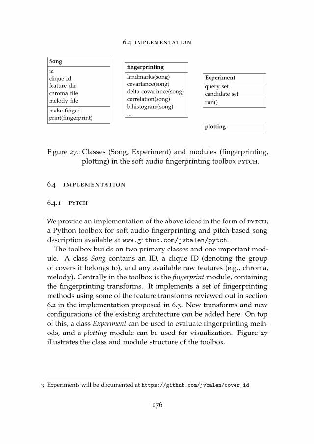
Figure 27.: Classes (Song, Experiment) and modules (fingerprinting,plotting) in the soft audio fingerprinting toolbox pytch.

6.4 implementation

6.4.1 pytch

We provide an implementation of the above ideas in the form of pytch,a Python toolbox for soft audio fingerprinting and pitch-based songdescription available at www.github.com/jvbalen/pytch.

The toolbox builds on two primary classes and one important mod-ule. A class Song contains an ID, a clique ID (denoting the groupof covers it belongs to), and any available raw features (e.g., chroma,melody). Centrally in the toolbox is the fingerprint module, containingthe fingerprinting transforms. It implements a set of fingerprintingmethods using some of the feature transforms reviewed out in section6.2 in the implementation proposed in 6.3. New transforms and newconfigurations of the existing architecture can be added here. On topof this, a class Experiment can be used to evaluate fingerprinting meth-ods, and a plotting module can be used for visualization. Figure 27

illustrates the class and module structure of the toolbox.

3 Experiments will be documented at https://github.com/jvbalen/cover_id

176

6.4 implementation

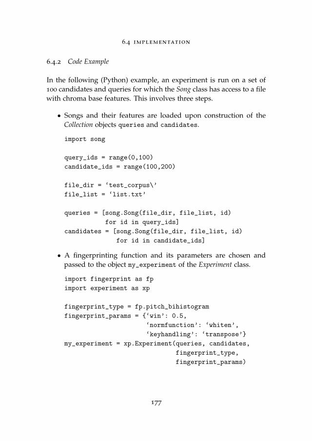
6.4.2 Code Example

In the following (Python) example, an experiment is run on a set of100 candidates and queries for which the Song class has access to a filewith chroma base features. This involves three steps.

• Songs and their features are loaded upon construction of theCollection objects queries and candidates.

import song

query_ids = range(0,100)

candidate_ids = range(100,200)

file_dir = ‘test_corpus\’

file_list = ‘list.txt’

queries = [song.Song(file_dir, file_list, id)

for id in query_ids]

candidates = [song.Song(file_dir, file_list, id)

for id in candidate_ids]

• A fingerprinting function and its parameters are chosen andpassed to the object my_experiment of the Experiment class.

import fingerprint as fp

import experiment as xp

fingerprint_type = fp.pitch_bihistogram

fingerprint_params = {‘win’: 0.5,

‘normfunction’: ‘whiten’,

‘keyhandling’: ‘transpose’}

my_experiment = xp.Experiment(queries, candidates,

fingerprint_type,

fingerprint_params)

177

6.4 implementation

• Finally, the experiment is run. The experiment is small enoughfor the system to compute all pairwise (cosine) distances be-tween the fingerprints.

my_experiment.run(dist_metric=‘cosine’,

eval_metrics=[‘map’])

print my_experiment.results

In most practical uses of this toolbox, it is advised to set up a newmodule for each new dataset, overriding the Song and Experiment con-structors to point to the right files given an ID. In the future, an indexmay be added to store and retrieve fingerprint hashes for large collec-tions.

6.4.3 Example Experiment

We now demonstrate in an example experiment how bigram-basedfingerprints can be compared, by testing a number of configurationsof the system in a cover song retrieval experiment.

As a dataset, we use a subset of the Second Hand Song dataset of1470 cover songs.4 The subset contains 412 ‘cover groups’ or cliques,and for each of these we have arbitrarily selected one song to be thequery. The other 1058 songs constitute the candidate collection. Sincethe subset is based on the second hand song dataset, we have accessto pre-extracted chroma features provided by the Echo Nest. Thoughnot ideal, as we don’t know exactly how these features were computed(see section 3.4), they make a rather practical test bed for higher-levelfeature development.

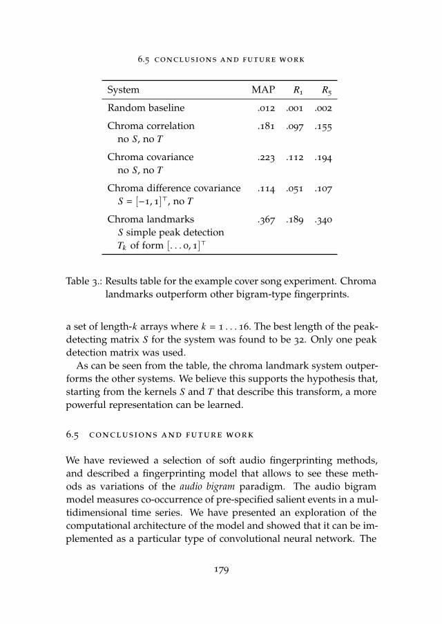
We implemented four bigram-based fingerprints: three kinds ofchroma co-occurrence matrices (correlation, covariance, and chromadifference covariance following [90, 191]), and one chroma landmarksystem, roughly following [12]. The results, with a description of thekernels S and T , are given in Table 3. The chroma landmark strategywas optimized over a small number of parameters: Tk was settled on

4 http://labrosa.ee.columbia.edu/millionsong/secondhand

178

6.5 conclusions and future work

System MAP R1

R5

Random baseline .012 .001 .002

Chroma correlation .181 .097 .155

no S, no T

Chroma covariance .223 .112 .194

no S, no T

Chroma difference covariance .114 .051 .107

S = [�1, 1]>, no T

Chroma landmarks .367 .189 .340

S simple peak detectionTk of form [. . . 0, 1]>

Table 3.: Results table for the example cover song experiment. Chromalandmarks outperform other bigram-type fingerprints.

a set of length-k arrays where k = 1 . . . 16. The best length of the peak-detecting matrix S for the system was found to be 32. Only one peakdetection matrix was used.

As can be seen from the table, the chroma landmark system outper-forms the other systems. We believe this supports the hypothesis that,starting from the kernels S and T that describe this transform, a morepowerful representation can be learned.

6.5 conclusions and future work

We have reviewed a selection of soft audio fingerprinting methods,and described a fingerprinting model that allows to see these meth-ods as variations of the audio bigram paradigm. The audio bigrammodel measures co-occurrence of pre-specified salient events in a mul-tidimensional time series. We have presented an exploration of thecomputational architecture of the model and showed that it can be im-plemented as a particular type of convolutional neural network. The

179

6.5 conclusions and future work

model can therefore be optimised for specific retrieval tasks using su-pervised learning. Finally, we have introduced an implementation ofthe model, pytch.

As future work, we plan a more extensive evaluation of some of theexisting algorithms the system is capable of approximating. Standarddatasets like the covers80 dataset can be used to compare results to ex-isting benchmarks. If the results are close to what the original authorshave found, pytch may be used to do a comparative evaluation thatmay include some variants of the model that have not previously beenproposed.

We also intend to study the extent to which the convolutional net-work implementation of the model can be trained, and what kind ofvariants of the models this would produce. This can be done mosteasily using the complete Second Hand Song dataset, because a ratherlarge number of train and test data will be required.

180