1991 GoodTuringSmoothing-A Comparison of the Enhanced Good-Turing and Deleted Estimation Methods for Estimating Probabilities of English Bigrams

Computer Speech and Language (1991) 5, 19-54

A comparison of the enhanced Good-Turing and deleted estimation methods for estimating

probabilities of English bigrams

Kenneth W. Church and William A. Gale AT&T Bell Laboratories, Murray Hill, New Jersey 07974, U.S.A.

Abstract

In principle, n-gram probabilities can be estimated from a large sample of text by counting the number of occurrences of each n-gram of interest and dividing by the size of the training sample. This method, which is known as maximum likelihood estimator (MLE), is very simple. However, it is unsuitable because n-grams which do not occur in the training sample are assigned zero probability. This is qualitatively wrong for use as a prior model, because it would never allow the n-gram, while clearly some of the unseen n-grams will occur in other texts. For non-zero frequencies, the MLE is quantitatively wrong. Moreover, at all frequencies, the MLE does not separate bigrams with the same frequency.

We study two alternative methods. The first method is an enhanced version of the method due to Good and Turing (I. J. Good [1953]. Biometrika, 40, 237-264). Under the modest assumption that the distribution of each bigram is binomial, Good provided a theoretical result that increases estimation accuracy. The second method is an enhanced version of the deleted estimation method (F. Jelinek & R. Mercer [1985]. IBM Technical Disclosure Bulletin, 28, 2591-2594). It assumes even less, merely that the training and test corpora are generated by the same process.

We emphasize three points about these methods. First, by using a second predictor of the probability in addition to the observed frequency, it is possible to estimate different probabilities for bigrams with the same frequency. We refer to this use of a second predictor as “enhancement.” With enhancement, we find 1200 significantly different probabilities (with a range of five orders of magnitude) for the group of bigrams not observed in the training text; the MLE method would not be able to distinguish any one of these bigrams from any other. The probabilities found by the enhanced methods agree quite closely in qualitative comparisons with the standard calculated from the test corpus.

Second, the enhanced GooddTuring method provides accurate predictions of the variances of the standard probabilities estimated from the test corpus. Third, we introduce a refined testing method that enables us to measure the prediction errors directly and accurately and thus to study small differences between methods. We find that while the errors of both methods are small due to the large amount of data that we use, the enhanced Good-Turing method is three to four times as efficient in its use of data as the enhanced deleted estimate method.

0885-2308/91/010019+36 SO3.00/0 0 1991 Academic Press Limited

20

Good- Turing metllod is preferable to the enhanced deleted estmute method. Both methods are much better than MLE.

1. Introduction

I. I. Possible applications oj’ bigram ,freyuencirs

A planned use of bigram frequencies is for disambiguation of the output of an optical character recognizer designed by Baird (Kahan. Pavlidis & Baird, 1987). Consider these two simple examples. In each case, suppose the recognizer has assigned about equal probability to having recognized “farm” and “form,” having used both the unigram frequencies and the optical information. In one case, the two possibilities including adjacent words are:

federal farm credit federal form credit

In the other case. the two pcjssibilities are:

some form of some farm of

We doubt that the reader ha,3 any trouble specifying which alternative is more likely. By using the following conditlonal probabilities based on the eight bigrams in these sequences, a computer program can rely on an estimated likelihood to make the same distinction. The conditional probabilities are for the word other than ,form or farm

conditional on form orfarm. They are calculated by dividing the bigram probabilities by the unigram probabilities for,form, 3683/2.2 x 10’. and for farm, 4563/2.2 x 10’.

Bigram Probability x

federal farm 0.50 federal form 0.039 farm credit 0.13 form credit 0.026 some form 4.1

some farm 0.63 form of 34. farm of 0.81

106 Conditional

probability x IO3

2.4 0.23 0.63 0.16

34. 3.0

200. 3.9

The deciding scores will then be found by multiplying the conditional probabilities based on the two constituent bigrams. This is only exact if the bigrams are independent. but it is useful in any case. For the first example, the scores so generated are (2.4 x 10-j) x (0.63 x IO-‘)= 1.5 x 10-6, and (0.23 x lo-‘) x 0.16 x lo-“)=0.037 x 10mh. The ratio of these shows that the reading “farm ” is 40 times as likely as the reading “form” in the first context. In the second context, the reading “form” is 410 times as likely as “farm.” This exam:>le shows how likelihood ratios based on bigram probabili-

Estimating probabilities of English bigrams 21

ties derived from a corpus of English text can be used to disambiguate optically confusable minimal pairs.

A similar application is the disambiguation of confusable pairs in a speech recognition system. Other applications include refining proof reading tools, such as the Writer’s Workbench (Cherry, 1981). For example, while spelling programs have proven quite useful, many spelling errors produce another word. A program with bigram probabilities could use context to detect legal words in unlikely contexts. Labeling parts of speech is useful for proof reading tools, and one method, Church (1989), relies on estimates of probabilities of trigrams of parts of speech. Sproat and Shih (1990) relies on bigrams of Chinese characters. In addition, bigram probabilities could be used to support lexico- graphic research, by identifying “interesting” pairs of words in a particular topic relative to general use (Church & Hanks, 1989). There are more applications in information retrieval; the ability to identify the pairs common within a given document but generally uncommon provides a way to locate documents similar to a given document.

Applications are discussed further elsewhere (e.g. Church et al., 1989); the work reported here develops and tests two methods.

1.2. Possible uses for variances

This paper uses variances of bigram estimates to compare methods. Other applications are possible. For instance, suppose a lexicographer wishes to identify words used with the word “potatoes.” The following table shows some bigrams which end with “potatoes,” ranked by t-scores comparing the joint probability of the bigram to chance. Variances are required to calculate the t-scores.

Word-l Word-2 t

sweet mashed

and couch of frozen fresh small baked

potatoes 4,6

potatoes 4.3 potatoes 4.3

potatoes 4.0 potatoes 3.8 potatoes 3.3 potatoes 3.3

potatoes 2.8 potatoes 2.8

potatoes 2.1

It should be clear that the variances allow the lexicographer to identify many words of interest, easily. Pairs with higher scores are more likely to be interesting pairs, so the lexicographer will find more interesting pairs in a given amount of time by examining the pairs in the order of the t-scores than by using a random order.

1.3. The failure of the maximum likelihood estimator (MLE)

Suppose that a particular pair of words occurred r times in a sample of N pairs of the language. The obvious estimator of the probability of the pair is r/N. This estimator is in fact the maximum likelihood estimator if the occurrence of the pair of interest is a random variable with a binomial distribution.

22 K. W. Church and I+‘. .4. C&de

The problem is that most possible pairs will not occur in a given sample, because. as shown in Section 2, the square of the vocabulary size greatly exceeds the number of words in the corpus. Therefore, most of the possible pairs have an observed frequency

r=O. However, as our example shows, we wish to take products and ratios of the estimated probabilities, and it will often happen that neither of two alternative bigrams

has been seen in the training text. In this case, the MLE would not determine a likelihood ratio, as both probabilities would be estimated at zero. Furthermore, even the same

estimate for all the unseen bigrams is seriously misrepresentative. since our work shows predictable factors of a million among the probabilities of unseen bigrams.

The maximum likelihood estimates of variances are also biased, because the estimates for the probabilities are severely biased. In particular, no estimate of the variance is available for bigrams not seen in the training corpus.

1.4. Some alternatives that have been suggested

We consider methods that tackle this problem by adjusting the observed frequency. Let r* be the adjusted frequency for a type observed r times. Then p, the probability of the type, is estimated by r*/N. In order to satisfy the constraint Cp= 1. the adjusted frequencies must satisfy

=N,r* _ , N

Johnson (1932) and Jeffreys (1948) proposed statistically motivated approaches. John-

son suggested adding some constant k to the frequency for each type and renormalizing appropriately. That is, the adjusted frequency, r *, is r + k times a renormalization factor,

N/(N+ kS), where S is the total number of types. The assumptions for this to hold are the most bland for k = I, which was Jeffrey’s suggestion. This is also an extremely common engineering approach, as it just calls for adding one to each r. We have treated this suggestion in detail elsewhere (Gale & Church, 1990), and do not consider it here.

The IBM speech recognition group has found the formula introduced by Good (1953) and attributed to Turing to be a useful estimator in building a language model for speech recognition applications (Nadas, 1984, 1985; Katz, 1987). They also introduced held out and deleted estimation methods. We define and illustrate each of these three methods in the next section. Katz is responsible for the term “backing-off,” which we have adopted, to indicate the process of building an n-gram model based on an (n - I)-gram model. Katz suggested using the GooddTuring estimator to build from a unigram model to a bigram model and on to higher n-grams. We have adopted this backing-off approach of extending an n-gram model to an (n + 1 )-gram model, although the methods we study are novel. Katz also used the following two approximations of the Good-Turing method, motivated by constraints on processing capability. First, for r > k (specifically, k = 5), set r* = r. Second. treat the bigrams observed just once as if they were unobserved.

2. Selection of materials for testing estimation methods

Our corpus was selected from articles distributed by the Associated Press newswire in 1988, which we refer to as the “AP wire.” Some portions of the year were lost. The remainder was processed automatically (Liberman & Riley, 1988) to remove identical or


nearly identical articles. There remained N= 4.4 x lo7 words in the corpus. The AP wire may not be sufficiently representative of English as a whole to use bigram frequencies derived from it in applications. However, as a means of testing methodologies, a large corpus size is desirable, and it is much larger than alternatives such as the Brown Corpus.

We split the 1988 AP wire into two portions, one for estimating probabilities and one for testing the estimates, and simply consider our universe to be the 1988 AP wire, rather than English. We made the split by assigning each bigram randomly with equal probability to one of the two portions. It is important that we made this split at random, because the topics discussed in the AP wire generate measurable differences in bigram frequencies over the period of a month. By taking random bigrams, we generate as close to two samples of the same universe of discourse as possible. If we had split the 1.988 corpus into two six-month subcorpora, then there would be measurable differences between the two subcorpora, as will be shown in Section 8.

What is a “word”? Roughly speaking, a word is a string of characters delimited by white space. For instance, “The” and “the” are different words, and “need” and “needs” are also. Punctuation modifies this definition: period, comma, hyphen and other punctuation marks were treated as words. Additional tokens were inserted automatically to delimit sentences, paragraphs and discourses. These definitions resulted in a vocabulary size, V, for 1988 of 400 653 words, or for the training sample, of 273 266. The resulting vocabulary size is two orders of magnitude larger than the 5000 words reported for the IBM speech recognizer (Nadas, 1984).

Our goal is to develop a methodology for extending an n-gram model to an (n+ l)- gram model. We regard the model for unigrams as completely fixed before beginning to study bigrams. This includes specifying the vocabulary, V, and an estimate, e(p(x)), of the probability, p(x), of each word, x, in V. We also suppose that the variances of the estimates in the unigram model are known. Likewise, we would regard a bigram model as fixed before studying a trigram model.

3. The basic Good-Turing and deleted estimation methods

This paper studies two alternatives to the MLE, which we call Good-Turing (GT) estimates and deleted estimates (DE). This section defines what we mean by “basic” variants of each of these methods. The equations and notation introduced here are summarized in Appendix B.

The Good-Turing estimator may be familiar to some readers from its applications in population biology. The key insight suggested by Turing and developed by Good (1953), is the use of N,, the number of bigrams which occur r times. We may refer to N, as the frequency of frequency r. The entire distribution {N,,,N,,N,,. . .} is available in addition to the particular r. The Turing estimator uses this extra information as r* = (r + l)N,+ ,/N,. Good suggested smoothing the observed N, to provide a sequence {S(N,)} for use in the formula, and discussed a number of possible smoothing approaches. We call r* a basic Good-Turing estimator (BGT) when smoothed N,s are used. Many different basic Good-Turing estimators are possible depending on how the smoothing is performed. A derivation of Turing’s formula is given in Appendix A. The proof there shows that the Good-Turing equation rests on the assumption that the distribution of each bigram is binomial.

Table I may clarify the the use of the Good-Turing estimator. The first column of the

24 K. W. Church und W. A. G&J

TARL.F I. Basic Good-Turing method combmed frequrncles ot blgr;rma

I’ (=MLE) h’, !* (=BGT)

74671 100000 0~0000270 2018046 0,446

449 72 I I ,2i

188 933 7.74 __ 105 668 3.24

68 379 4.2

48 190 5.1’)

35 709 h,?l 27710 7.34

33 3x0 -2. _ X.25

table shows frequencies of bigrams from zero through nine. (For this example, we are using small frequencies, r, with large N, so that we do not need to discuss smoothing the N,s.) This column is also the MLE, of course. The second column shows N,. how many bigrams had those frequencies in a training sample of about 22 000 000 bigrams, which was half of the 1988 AP wire. For instance. 2 018 046 bigrams appeared exactly once in the sample. The third column shows the adjusted frequencies as calculated by the Turing

formula. The adjusted frequencies, r*, can be compared to the raw frequencies, Y. They

have the same order, and do not differ greatly. The method assigns some probability to bigrams which have not been seen, suggesting that we should act as if we had seen each of them 0.0000270 times instead of zero times. In order to compensate for moving 7.47 x 10’” bigrams from 0 to 0.0000270, some larger frequencies must be adjusted downwards. In this case, the adjusted frequencies, r *. for all observed bigrams are less than the corresponding raw frequencies, r.

Notice that the calculations for r = 0 rests on knowing N,, the number of bigrams that we have not seen. We can calculate this because we know the vocabulary size, V. from the unigram model. (This marks a great difference in our application of the Good- Turing formula from the kinds of applications made in population biology. where

inferences about the population size are the desideratum.) The total universe of bigrams that we wish to know about has size V’z 1.6 x 10”. N,, is the difference between V’ and the number of distinct bigrams seen,

Note that N,,c V’ since

NC,= V-EN, and xN,<N< C” r>O r>O

In other words, hardly any of the possible bigrams have been seen. The Good-Turing estimator is based on a theorem about the expected frequency in an

additional sample of bigrams which occur r times in the observed sample. An empirical realization of this idea is the held out estimator defined by Jelinek and Mercer (1985). Let the available text be divided into two halves. called retained and held out. For each


bigram, b, let r,(b) be its frequency in the held out half of the text. Let the number of distinct bigrams with frequency r be

NT=1 1 blq(b)=r

Then count all occurrences of all the bigrams with frequency r in the held out half of the text,

blq(b)=r

where the r,(b) is the observed frequency of the bigram, b, in the held out half. The adjusted frequency is r* = CJN,. We use the held out method, with the training half of

the bigrams as retained and the test half of the bigrams as held out, for the standard against which we compare any other method. This standard is the only estimate with access to the test part of the data; all other methods are restricted to the training part. Again, when applied to all the data, we refer to this as the “basic” held out method (BHO). The only assumption behind this method is that the same process generates both halves of the text. This assumption is much weaker than the binomial assumption of GT.

Table II may clarify the calculations in the held out method. The first two columns are as in the previous table. The third column gives the extra information collected for the held out method, C,, and the fourth column gives the basic held out estimates, C,/N,. The adjusted frequencies for the BGT can then be compared to the adjusted frequencies for the BHO as well as to the MLE. Apparently, the BGT is better than the MLE since the differences between the BHO and the BGT are limited to the third significant figure,

while the differences of either from the MLE are in the first significant figure.

Applying the held out method between two halves of the training data would give another potential method. A more efficient use of the training data is made by the deleted estimate defined by Jelinek and Mercer (1985). Essentially, this is a way to combine held out estimates made by interchanging the roles of held out and retained halves of the text. Denoting the two halves of the training data by 0 and 1, we have NF is the number of

TABLE II. Basic held out method

r (=MLE) N, c, BHO (= standard)

0 74 67 1 100 000 2019 187 0.0000270 1 2018046 903 206 0.448 2 449 721 564 153 1.25 3 188 933 424015 2.24 4 105 668 341099 3.23 5 68 379 281776 4.21 6 48 190 251951 5.23 I 35 709 221693 6.21 8 27 710 199 779 7.21 9 22 280 183 971 8.26

‘6 K. W. Church and U’. A. Cfalr

bigrams occurring r times in the half labeled 0, and C :” IS the total number ot occurrences in the half labeled 1 of those bigrams. Likewise, Nj is the number of bigrams occurring r times in the half labeled I, and CI” is the total number of occurrences in the half labeled 0 of those bigrams. The two held out estimators would be C’y’ ‘N,’ and C!” NI. The more efficient deleted estimate is formed by combining these quantities by

The basic deleted estimate (BDE) is formed by applying this method to the entire data, as shown in Table III. The BDE is much closer to the standard BHO than is the MLE:

however, it is not as good as the BGT. It differs in the first significant figure for r = 0, and in the second significant figure for several other values of r.

4. The enhanced methods

A key suggestion of this work is the introduction of a second predictor of frequency of observation in addition to an observed frequency; accounting for the second predictor constitutes what we call an enhanced method. We study an enhanced Good-Turing method and an enhanced deleted estimate method. We compare each to an enhanced

held out estimate as the standard. Both enhanced methods allow us to dzfirentiate among the many bigrams which have not been seen. We will show that about 1200 significantly different probabilities can be estimated for bigrams not seen in the training

text. Thus the probabilities estimated by the enhanced Good-Turing method and the enhanced deleted estimate method for the unseen bigrams are neither zero nor identical. We will refer to either method used without a second variable as a “basic” method.

The backing-off approach to a bigram model regards a bigram as a pair of unigrams (words). Supposing we had no empirical information on a bigram frequency, we might still hazard a guess as to the bigram’s probability based on characteristics of the words in the bigram. The basis for this guess becomes a second predictor when empirical

frequency information is available. We build a bigram model by applying a basic method within each category of bigrams grouped by the second predictor. The application of

TABLE III. Basic deleted estimate method

Y

0 35821500000 1 366 260 36413 100000 1 336 639 0~0000374 1 1 342 199 540 946 1 356 307 528 932 0.396 7 266 824 336 463 268 783 328 675 1.24 3 110 187 249 294 111 849 244 943 2.23 4 61065 199 868 62 243 197 510 3.22 5 39 173 167 895 39 933 165 639 4.22 6 27 823 146 663 28 275 144 787 5.20 7 20 666 130 046 20 946 128 537 6.21 8 16 131 117573 16 135 113962 7.18 9 13002 108 043 12 767 102 656 8.18

C-g’ N! Cl” BDE


Turing’s formula is valid in this case because the population of bigrams is prespecified; it depends only on the unigram model.

4.1. Unigram estimates: a second predictor

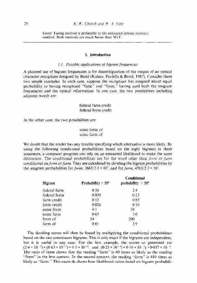
A possible second predictor for bigrams is the following. If the text were composed of independently generated words, then the probability of a pair of words would just be the product of the probabilities of the individual words. Of course, the words are not independently generated, but the frequency predicted on this basis is still a useful predictor, as shown in Fig. 1.

Let jii=iVe(p(x))e(p(y)) be the predicted frequency if the words, x and y, were independently distributed with the probabilities estimated by the unigram model as e(p(x)) and e(p(y)). Since the population probabilities, such asp(x), are estimated by the unigram model, we refer to values of jii as unigram estimates (UE) when we compare them to other estimates, such as MLE or EGT. We assume that the unigram model provides variances of the estimates as well as the estimates. Our unigram model uses maximum likelihood estimates, and the vocabulary is taken as the oberved vocabulary in the training set. A more elaborate treatment of the unigram model would use Good-

-6-.*

log,,, expected frequency if independent (ii;)

Figure 1. A second useful predictor of bigram frequencies. Enhnncemenf of the Good-Turing or deleted estimate methods consists of using the basic methods on categories defined by a second predictor. The second predictor used in this paper is the frequency with which we would expect to see each bigram if each word of the text were selected independently, which we denote here by jii, acronym for “joint if independent.” Its logarithm (base 10) is shown as the abscissa. The ordinate is the average of observed frequencies for words grouped by jii. The figure shows that the average frequency is strongly correlated with the independent frequency over about 10 orders of magnitude.

28 K. W. Church und W. .4. Gale

Turing estimates and allow for words not seen in the tratmng set. We compare the accuracies of the methods on those bigrams composed of words seen in the training set.

Other predictors could be used for the grouping;jii is one of many possibilities. We do not know what makes one variable better than another for grouping. A necessary property of the grouping variable is that it be possible to count the number of types included in each group, because we need to know N,!. We hypothesize that if one variable predicts r better than another. then it will make a better grouping variable. It is useful for

smoothing that .jii is a continuous variable.

4.2. Enhanced methods

We use enhanced versions of the held out, deleted estimation and Good-Turing

methods. The basic versions of these methods were defined in the previous section. The enhanced versions of each are defined using data collected by both frequency, r. and jii bin, j.

The standard is now the enhanced held out (EHO, or STD) estimate, r* = C,,i’A’;,. where N, is the number of bigrams with frequency= r in the training sample and jii bin =j based on the unigram model, and C,r is the observed count in the test corpus of bigrams with frequency = r andjii bin =,j. The enhanced Good-Turing (EGT) estimate is r* = (r+ l)S(N,,+ ,)/S(N,,), where the smoothing, S, is over r for a fixedj. as described in the following subsection. The enhanced deleted estimate (EDE) is r* = (Cg’ + C::))/ (N:l+ NJJ, where the superscripts, 0 and 1, refer to two halves of the truining sample. Cpr

and C’:p are the observed counts in a second (first) half of the training corpus of bigrams with frequency = r in the first (second) half. and Nf, and N:). are the number of types in

the first (second) half of the training corpus with frequency r in the half corpus and jii bin =j. Notice that the meaning of r changes in this method to a frequency in half of the training corpus, but is then used to estimate probabilities for bigrams with frequency r in the entire training corpus. We believe this discrepancy accounts for the systematic problems this estimator has for small r.

4.3. Smoothing methods

We have introduced two variables r and jii, for predicting frequency observations. Practical methods may need smoothing across these variables. We find that both deleted estimation and Good-Turing need smoothing across,jii, while GooddTuring also needs smoothing across frequency, r.

The smoothing across jii is accomplished by controlling the size of the categories, or bins, derived from the continuous variable. There is a trade-off between specificity ofjii and smoothness in selecting how manyjii groups to use. Using fewer bins induces more smoothing; more bins less smoothing. We use about 35 groups, taking three groups in each factor of 10. We have not studied this trade-off more than to note that IO groups per order of magnitude ofjii gave results that we kept feeling a need to smooth, so we went to three groups per order of magnitude.

After dividing all the bigrams into groups, we calculate N,,,, the number of distinct bigrams in each group, so that we can calculate the number of bigrams not seen. The calculation of the Nj,i is made as follows. For each pair (r,,rJ of observed frequencies of the unigrams, determine jii=r,rJN. From that determine the bin for jii, and add the


product of the number of distinct unigrams seen with the two frequencies to the cumulating count for that bin.

Let N,r be the frequency of frequency r in jii bin j. Figure 2 is a plot of N,, for r = 0,1,2,3 as a function of jii. The plot shows that N,, has a qualitatively different shape than do N,, for r= 1,2,3. For the higher values of r, omitted for the sake of clarity in the figure, the plots resemble those for r= 1,2,3. For the smoothed values of N, required by the enhanced Good-Turing method, we treated r= 0 separately, and smoothed log(N,,) against log(jii). For r > 0, we smoothed log(N,) against log(r).

Figure 3 shows logarithms of Njr versus logarithms of r for j= 22. The non-zero raw values are plotted in the left panel. Since most of the N,, are zero for large r, we need to account for them. Good used groups of frequencies. We average each non-zero N, with the zero Nj, that surround it: order the non-zero Nj, by r, and let q, r and t be successive indices of non-zero values. Then replace N,, by N,lO.5(t - q). In other words, we estimate the expected Njr by the density of Nir for large r. For small r. there is no change because the length of the interval is one. For large r, the change can make a difference of up to four orders of magnitude. Figure 3 shows before and after plots for the 22nd group for which we would predict a frequency, jii, of I.4 observations per 22 million words, if the words were independent. The averaging can be seen to restore the downward trend that is clear in the region with low quantization noise. The noise in the averaged data, and the sensitivity of the Good-Turing formula to slopes among the N, or S(N,) shows the necessity of a smooth for all but the smallest r. Without averaging and smoothing, most of the N, are zero for large r. Thus, the calculation N,+,/N, would be grossly wrong.

log,,, (iii) = loglo frequency it words independent

Figure 2. Numbers of distinct bigrams. The bigrams are divided into groups according to the logarithm of jii, three groups per factor of IO. This figure plots N,,, the number of distinct bigrams observed with frequency r within the jii binj, for r = 0,1,2,3 as a function of log,,(jii). Notice that Np is qualitatively different from Ni, for other r. We treat it separately in the following analysis.

K. W. Church und W. A. G&J

-2

L I I I

0 I 2 3

-_-_-_ .------ .~ ------- (b)

log,0 frequency ( r )

Figure 3. Averaging zeros and smoothing. (a) Shows logarithms of raw non-zero N,, against logarithms of I > 0, for a fixed bin Cjii- I .4). Each point represents one value of r. (b) Shows the raw N(, averaged in with ail the N!, which are zero. The result is nearly linear over three orders of magnitude m r. We use a smoother that adjusts the amount of smoothing locally to take account of the change from low variance data for small r to high variance data for large r. The smoother also guarantees a smooth first derivative. The result of smoothing is shown by the solid line.

The smoother we use, described by Shirey and Hastie (1988) has two useful properties for this application. First, it uses a technique called local cross validation to determine the range of data to smooth. The values for small r get very local smoothing, while for large r, nearly all the data is used. Second, the smoothness of the first derivative can be directly controlled, and we require it to be quite smooth. We make this requirement

because we want to use Nj(,,,,/Nj,, w ic h h . IS essentially a derivative with respect to r.

5. Testing the enhanced Good-Turing and deleted estimate methods

The assumptions of the Good-Turing theorem may seen innocuous: a finite set of types and a marginally binomial distribution. The first assumption (finiteness) was satisfied by construction. But the second assumption is not; we know that word sequences are not independent. There are considerable correlations within any discourse. Thus. we need to test how well a method assuming a marginally binomial distribution works in practice.

In this section we will be comparing six estimates and their variances for bigram probabilities. These six estimators are the standard (STD), the maximum likelihood estimator (MLE), the basic Good-Turing estimator (BGT), the unigram estimator (UE), enhanced deleted estimate (EDE) and enhanced Good-Turing (EGT). The section has two subsections in which we first compare the five estimates qualitatively, then introduce the variances of the estimates and compare these qualitatively. In the next section we use the variances to make a delicate quantitative comparison.


5.1. Qualitative evaluation of the methods

We find that the Good-Turing estimates and the deleted estimate estimates agree very

well with the standard estimates over the entire range of data that we can test. The smallest frequency observations are the most critical. Figure 4 shows the results for r = 1. The deleted estimate and Good-Turing estimates can be viewed as combining the MLE and UE, and indeed, these “combined” estimates usually lie between the two long

dashed lines. Figure 5 presents a plot similar to Fig. 4 for the important case of r = 0. Figure 6 shows

similar plots for r= 2, 5, 8, 11, 14 and 17.

For frequency zero, the range of probabilities in STD is about six orders of magnitude, five orders of magnitude larger than for any other frequency. Over this range, EGT agrees well with the standard estimates, deviating systematically for the smallest jii, however. EDE agrees reasonably well, but is systematically too high over most of the range.

Note that r* depends more on jii when r is small; the slope of r* is very steep for r = 0, and pretty flat for r = 17. This means that UE is more important when r is small. We will return to this when we consider the number of significantly different probabilities. After

2.0 - UE I

* I 1 c I I L

c ! ’

EOE I I

; I ’ i 1 I 1.5-

I

2 m a

; ._ MLE P ,.O_-_----- ---- -- :

P

0.5 - BGT 1 -6 -4 -2 0 2 4

log,o jii

Figure 4. Enhanced Good-Turing and deleted estimate agree with the standard for r= 1. Six predicted frequencies are shown in this and following figures: (1) the standard, STD, shown by points; (2) the maximum likelihood estimate, MLE, shown by long dashes; (3) the unigram estimate, UE, shown by long dashes; (4) the basic Good-Turing method, BGT, shown by a solid line; (5) the enhanced deleted estimate, EDE, shown by short dashes; and (6) the enhanced Good-Turing estimate, EGT, shown by solid lines. These estimates are plotted against the logarithm of the unigram estimator, jii. Note that EDE and EGT agree closely with the standard. They are quite distinct from either the MLE or UE but lie approximately between these two primary estimators. Any basic method, such as BGT or MLE, is bound to miss dependence on jii.

-6

Figure 5. Enhanced t~ood Turing and deleted esttmatc agree with the standard for r= 0. Note that S I D and EGT agree closely. EDE is systematically high BGT totally misses the variation with jii. of course, and for r=O with SIX orders of magnitude of variation. the lack is extreme. The MLE of 0 cannot be plotted on a logarithmic scale. UE overestimates by a I‘dc:or elf about three

examining the variances of predicted frequencies in the next section, we will return to quantitative comparisons.

Our standard is an empirica’ measurement. and consequently. some differences from the standard are to be expected oy chance. We need to estimate the variance of the standard in order to assess the significance of differences between EGT or EDE and the standard. This subsection shows how this variance can be estimated directly, and that the Good- Turing theory provides an e:.planation for the observations. The next subsection uses the

variances to compare the efkiencies of the estimators. The held out method can be used to calculate variances directly. The calculation for

11~~. the variance of observed frequencies about the mean for bigrams with frequency = I V and jii =,j is

where the sum is over bigrams, 6, such that r,(b)= r and jii=j. The Good-Turing theory also predicts this variance. Let ,y be the prediction. It is

composed of: (a) the variance of the true probabilities of the bigrams in the group about their mean; plus (b) the variance of observed frequencies for each group member about their expectations. Appendix A derives the following expression for the sum of these two terms:


-4 -2 0 2

lW,o Jil

Figure 6. Enhanced Good-Turing and deleted estimate agree with the standard for small r. Both EGT and EDE are much better than MLE and BGT. The difference is more important for small r. UE is only a plausible estimator for the smallest frequencies, say, r<2. (a) r= 2: (b) r= 5; (c) r= 8; (d) r= I I: (e) r= 14; (f) r= 17.

vy=r*(l+(r+l)*-r*)

Fig. 7 compares the observed and predicted variances for r = 1. Figures 7, 8 and 9 in this section have shown that there is good qualitative agreement

between the variances predicted by EGT and those observed as the standard. In the next section, we use GT variances to compare the differences of EGT and EDE from the standard estimates, since they are defined in more cells than are the directly estimated

variances.

6. Quantitative comparisons of Good-Turing and deleted estimate methods

The differences between the methods we are testing and the standard are so small that we need good microscopes to examine them. This section uses two such microscopes: comparison of the differences to standard deviations, and common scaling of the differences as entropies.

T

O-A -6 -4 -2 0 2

Figure 7. Enhanced Good-Turing variances agree with the standard for r-- I. Observed or predicted variances for the group of bigrams with r= I are shown as a function of IogCjir). The directly estimated variance of the standard is shown with points, and the variance predicted by EGT theory with lines. The EGT predictions follow the standard closely showing reliable estimates of the variance in estimation and observation.

-2 -

-4 -

* I I I / I

--b --4 -2 0 2 4

lOg,o J/l

J 4

Figure 8. Enhanced Good Turing variances agree with the standard for r = 0. Observed or predicted variances for the group of bigrams with r = 0 are shown as a function of logcjii). Predictions from EGT follow the observations closely.


8- 14 -

(0) (b) .

6- 12-

l * .

IO -

.

2.0

(Cl

. 18 -

16 -

x -6 -4 -2 0 2 -6 -4 -2 0 2 -6 -4 -2 0 2 4

24 - .

.

. .

22 -

32 - - (0) 38

.

36 -

Figure 9. Enhanced Good-Turing variances agree with the standard for small r. Predictions from EGT follow the observations closely. (a) r= 2; (b) r= 5; (c) r=8; (d) r= II; (e) r= 14, (f) r= 17.

6.1. Comparisons of precision and eficiency

One way to examine differences is to compare them to chance. Since we know the variances of the standard estimates, it is natural to compare other estimates to the standard estimates by comparing their difference to the variance: t,r = (r* - $I- For each jii bin, j, and each frequency, r, this equation defines a t-score, tjr, for the difference of an estimate, r*, from the standard estimate, r$ As explained in the previous subsection, we use the Good-Turing prediction of the standard’s variance, v,yT, because it matches the standard’s variance while being less noisy and defined in more cells.

While this t-statistic is directly a measure of precision, its importance lies in its efficiency implications. We will show that EGT is three to four times more efficient in its use of data than is EDE. That is, four months of data used by EGT methods will give

better accuracy than a year of data used by EDE methods. A perfect predictor would give t-scores distributed about mean zero with variance

one, because the variance of one standard observation is used as the denominator. We combine a group of these t-scores by taking the mean of the squares of the values, or the square root thereof, the root mean square (RMS). A perfect predictor would have a mean square of one, due to the observation variance of the standard.

For small frequencies we will have about 3.1 I-scores, one Ior each J?[ hln. I-~gure\ iti and Ii show two sets of these t-scores, and RMS summaries of them ,Ir 1’ = .i. the RMS

(root mean square,) t-score for EGT is 2.1 well above the unit\ that a perfect predictor ~ would achieve. The RMS t-score for the EDE method. 6.2. is even larger. howecer. because there is a systematic deviation from the standard over part of the range of jil.

Another frequency, Y= IO, is shown in Fig. I I. The RMS f-values are I ‘18 (EGT) and 2.4 (EDE).

Since the I-scores vary by frequency, r, we present a plot showing their RMS values as a function of r in Fig. 12. Each point in Fig. 12 summarizes a panel analogous to those in Figs 10 and 11. Dashed lines compare EDE with the standard while solid lines compare

EGT with the standard. We have several observations about Fig. 12. First, each of the methods has systematic

differences from the standard for the smallest frequencies, leading to large RMS f-values. Second, each of the two methods seems to settle down to a stable value by about r= 10, EDE to about 2 and EGT to very near the unity of a perfect predictor. Third. for each

frequency, EGT is better than EDE. The lower error rate of EGT can be translated into a greater etliciency-. The mean

square t-scores give a method’s variance normalized by that of the standard. In this setting, we can ascribe one unit of the normalized variance to the estimation errors in the standard. and the rest to errors in the method tested. On replication, however, other methods would share the same two sources of uncertainty generating the standard’s variance, as well as its own inherent sources of error. Thus the mean square l-scores represent the normalized variance that a method would have. on replication. for

. -5 -5

I .

I I I I I --~-__

I I 1

-6 -4 -2 0 2 4 6 -6 -4 -2 0 2 4

Figure 10. For I= 3. both EGT and EDE have errors larger than the standard enhanced Good- Turing and are better than deleted estimation. (a) Shows the plots of r-tests of the differences between EGT and the standard estimates. (b) Shows the plots of t-tests of EDE versus the standard. Lines are drawn at plus and minus the RMS (root mean square) of the r-values plotted. EGT shows no pattern to its differences, while their RMS is about 2.1. EDE shows a systematic difference from the standard for some values of.jii. leading to a larger RMS than shown by EGT.


I I

I 1 I I I I I I

I (b) ‘%

4

t ___- 2-

. . . .

l . . .

o- .

. l * .

. .

‘0

-2 - . _ . .

% .

. I I

0.

-6 -4 -2 0 2 4 6 -6 -4 -2 0 2 4

loglo jit

Figure 11. For r= 10, EGT approaches ideal performance while EDE has larger errors. Both (a) and (b) plot t-scores. as in Fig. 10, for r= 10. (a) Shows a performance near that of a perfect predictor, while (b) panel continues to show significant noise attributable to the predictor.

6

6

20 30 40 50

Frequency 1 r )

Figure If. Comparisons of the enhanced Good-Turing and deleted estimate methods, r < 50, Good-Turing is better than deleted estimation for all frequencies. Each point on these plots represents one panel such as shown in Figs 10 and 11. The plot shows the RMS f-value for frequencies, r, from one through 49 for EGT. The solid lines compare EDE with the standard; the short dashed lines compare EGT with the standard. The best performance theoretically possible is an RMS error of 1, shoan by the horizontal line. EGT has a smaller RMS z-value than EDE for each frequency.

6

38 K. W. Church und W. A. Guii~

estimating the bigram probabilities. Variance due to observation of‘ blnomlaiiy dlstrl- buted random variables will decrease in inverse proportion to the amount of data, however, so the ratios of mean square r-scores for two methods tell us the ratio of data

required by the methods to reach the same variance. The ratio of the mean square t-scores, MS(t~“)/MS(t~‘). is 16-3, for t’< 50. However,

this ratio is dominated by the systematic differences from the standard--~numbering

about 100 (rj) pairs for EDE and about 30 for EGT-which may not be reduced by collecting more data. Trimmed means, which discard the lowest and highest fractions of a set of data, allow one to look at the bulk of the data without distractions from the extreme values. The ratios of mean square l-scores using trimmed means vary from 3.7 for a 5% trimming fraction to 2.8 for a 20% trimming fraction. Thus the EGT is more efficient than EDE by a factor of three to four, as well as having fewer systematic errors.

It is worth emphasizing that the enhanced Good- Turing estimates are greatly superior to the MLE or any other basic method. Figure I3 makes this point by comparing the

RMS z-scores for MLE, BGT and EGT. The MLE and BGT improve in performance over the range shown, but do not reach

the level of EGT. The figure omits the MLE values for the smallest frequencies (for which the MLE has RMS t-values ranging from five to 30 times those of enhanced Good-Turing estimates) in order to show the comparison for larger frequencies more

”

I I I

IO 20 30 40

Frequency (r )

Figure 13. Comparing the enhanced Good-Turing, BGT and MLE methods. enhanced GoodPTuring is better, especially when r is small. Each point on this plot represents one panel such as shown in Figs 10 and 11. The plot shows the RMS r-values for frequencies, r, from 10 through 50. The solid lines show EGT, short dashed lines show BGT and long dashed lines show MLE. For r < 50, the RMS &scores for EGT are always less than those for BGT, which in turn are always less than for MLE. This results because the MLE and BGT do not distinguish among bigrams with the same frequency. r. This is particularly problematic when r=O. In the next section we show that the enhanced Good-Turing method is very good at distinguishing among bigrams that have not been seen (r=O).


clearly. The BGT and MLE t-scores are worse than those of the EGT because they do not distinguish among bigrams with the same frequency, r. The BGT is superior to the MLE because it averages across thejii differences, while the MLE is accurate only at the highest jii values.

6.2. Comparison of relative entropies

A common statistic reported for language models used for speech understanding is their entropy, H (Nadas, 1984; Katz, 1987), or equivalently, their perplexity, 2H. Entropy is defined by Katz for n-gram language models. For a bigram language model, M, the definition is

where w,, n= l,..., IV is the sequence of words in a test corpus, and P”(w,Iw,_,) is the model’s probability for the nth word given its precursor. By the definition of conditional probability, this can be rewritten as:

where P”(w,_ ,w,) is the model’s probability for the bigram w,_ ,w,, and P”(w,_ ,) is the model’s probability for the unigram w, _ , . The entropy of a language model, M, relative to the entropy of the standard is then:

MW w) PTD(W_,) =&$l”g2 (;&:;:,i,) PM(w,1,) 1

since the unigram models are the same for all the bigram models.

where the sum is over all bigrams (all pairs of unigrams), and freq(b) is the frequency of the bigram b in the test corpus.

40 K. W. Church und W. .I. Gulr~

where the sum is now over frequencies r in the training corpus. andJir btnsj defined from the unigram model, and C,r is the count of the corresponding bigrams in the test corpus.

Figure 14 shows terms in the sums for the EGT and EDE relative entropies when r = 1. The first panel in this figure is based on nearly the same information as is Fig. 4. which showed predicted frequencies for r= 1, although there are several changes. The first

I.5

0.5

,0.5

I .I__ I I I ’ . t

-6 -4 -2 0 2 4 6

12

i

.

(b) .

. IO .

.

2 2

6

t .

. 2 6 0,

i 4 t

. . .

-6 -4 -2 0 2 4 6

I I I I I I I I -6 -4 -2 0 2 4 ( 5

Figure 14. For r= I, EGT has relative entropy closer to zero than does EDE. The three panels show the calculation of the relative entropy: (a) shows logarithms (base 2) of probability ratios: (b) shows the weights with which these logarithms are combined; (c) shows the product of (a) and (b). Solid lines compare EGT and STD while dashed lines compare EDE and STD. EGT deviates less from zero than does EDE in the heavily weighted region.


change is that only the differences from the standard are shown. Another change is that logarithms of differences are shown instead of the differences, and indeed, the negative of the logarithmic difference is shown, so a low predicted frequency contributes positively to the relative entropy. Finally, each set of estimates is individually normalized to unit probability, which can result in the upward or downward shift of the line plotted in the panel.

Figure 14(b) shows that the relative entropy calculation weights some values of jii much more heavily than others. Only the middle range is important to this calculation. These are bigrams that the unigram model expects from once in 220 billion words to once in 2.2 million words. The resulting product in the third panel shows that the EGT method sticks closer to the standard over the heavily weighted frequency range.

The most important single frequency for the relative entropy calculation is r = 0. The detail for this frequency is shown in Fig. 15. Summing the entries shown in Fig. 1 S(c) gives the first two points in Fig. 16(a), while summing the entries shown in Fig. 14(c) gives the second two points.

Figure 16 shows that the weighted logarithmic differences are always smaller for EGT probabilities than they are for EDE. The relative entropies, which are the sums of the series shown in Fig. 16(c), are EGT: 0*0080 and EDE: 0.064. Since the contributions to these totals are always smaller for EGT than for EDE, and since the totals cannot be negative, it is quite reasonable to find h EGT less than hEDE. Of course, the relative entropies are all so small that they would not be important in an application. However, they are small precisely because we have used a large amount of data to estimate the probabilities here. The practical question is how much data is needed for a given level of performance. We believe that the relative variance calculation of the previous section provides a better guide to this question than does the relative entropy.

7. How many significantly different probabilities?

In this section we show that estimates in adjacent jii bins differ quite significantly. This implies that interpolation is justified, and leads to an estimate of the equivalent number of significantly different estimates.

For each jii, let 5, denote a frequency estimated for jii bin = j and frequency = r. The standard deviation of the difference, (&-Jj_ ,);), is ,/GjJNj,+ Ctj_ ,,,/NCj_ ,Jr, where N, is the number of types for jii = j and frequency = r, and sr are the Good-Turing variances for the frequencies predicted. Then the statistic we examine is the ratio

This is a t-score for sequential differences in the estimates and is a test of the significance of the differences between adjacent jii bins. Figure 17 shows the t-scores for the particularly important case of r = 0, the bigrams not seen in the training sample.

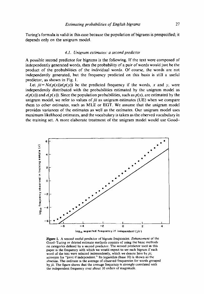
Figure 17 shows that for many jii values, the differences are highly significant. We estimate the equivalent number of significantly different values by taking the sum of all the t-statistics and dividing by l-65. For r= 0, the equivalent number of significantly different values is 1245. Figure 18 shows the equivalent number of significant differences as a function of frequency.

Figure 18 shows that the number of significantly different values falls rapidly from

42 I?. W. Church mu’ b. A. Gaie

-6 -4 -2 0 2 4 6

F . l l -

IO lb) . . eL .

3 2 . .

; 6

. .o

; 4 t

. .

Ll --b --4 -2 0 2 4 b

0.0 _--_

I’ I

I

,

/

t I

,’ -0.04 -

e :

P I I

I I

\ -0.06 - ’ I1

I I b

I I I I -6 -4 -2 0 2 4 c

Figure IS. For r=O. EGT has relative entropy closer to zero than does EDE. This figure shows the same panels as Fig. 14, for r = 0. It shows that the EGT probability estimate for r=O also stays closer to the standard than does EDE. in the region that is weighted heavily.

1200 as r increases, remaining above 1, however, for r ~40. For this range of r, then, there is some significant variation with jii. The decrease with increasing r is a consequence of the decreasing slope of the lines shown in Figs 4, 5 and 6, as r increases. The types of bigrams with frequency greater than 40 account for about 1.8% of types observed. Therefore, the splitting by jii is useful for about 98.2% of the observed bigram types and all of the unobserved bigram types. We conclude that enhancement is of considerable value for practical applications.

Estimating probabilities of English bigrams

I i I I I I I

(01 J 0 IO 20 30 40 50

1 L .

20

15

1

5 6 . 2 IO .P -I___ f

.

5 l

l . l **. tb)

l ***m .~***.*a**,*.*.

0 f T ..,...... . . . . . . . . . ,

0 10 20 30 40 5 0

I : I i I , I I u

0 IO 20 30 40 50

Fraqusncy (r )

Figure 16. For all r, EGT has relative entropy closer to zero than does EDE. Each point in (a) is the sum of series like those shown in Figs 14(c) and IS(c). The result is still a term in the contribution to the total relative entropy, and is now shown as a function of frequency. The weights in (b) show that the lowest frequencies are the most important individually for the relative entropy calculation. This figure shows that for each frequency, r, the EGT probability estimates are closer on average to the standard than are the EDE estimates. It is therefore not surprising ihat their sum, the relative entropy, is less for the EGT model than for the EDE model.

43

L

I I -6 -4 -2 0 2 4

lOill if,

Figure 17. About 1200 significantly different probabilities for r= 0. The horizontal axis shows the logarithm of&. The vertical axis shows r-statisttcs for the difference between successive values of the GoodPTuring estimates for bigrams not seen in the training text. The dashed lines are drawn at conventional significance levels of f 1.65. These differences are highly significant, showing that interpolation between the observed values is justified. Doing so would give the equivalent of using about 12OOjii bins.

8. Sampling, representativenes and extrapolation

We have shown that enhanced Good-Turing and enhanced deleted estimate predictions agree well with an observed standard. However, the training and validation texts were chosen to minimize discrepancies from these methods’ assumptions. This section argues that a training corpus needs to be carefully sampled to ensure representativeness, in order to make valid extrapolations. In support of this thesis we show that the language used in the first temporal half of our AP corpus is significantly different from the

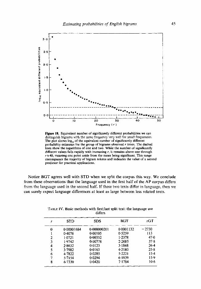
language used in the second half. Table TV shows basic Good-Turing predictions and an observed standard using the

first half and last half of our AP corpus as training and validation texts. The columns in this table are as follows: r is the frequency of bigrams in the training

text. STD is the standard held out estimate calculated with the first half as retained and the last half as held out. SDS is the standard deviation of STS, calculated as V,N,, where C’, is the variance of the group of bigrams. BGT is the basic Good-Turing estimate calculated from the first half. tGT is the t-score (BGT - STD)/SDS.

A striking feature in the table is the systematic differences between BGT and S, reflected in highly significant t-scores for their differences. These observations are to be contrasted with the behavior when we use random pairs to split the corpus, as shown in Table V.


0 IO 20 30 40 50

Frequency (r 1

Figure 18. Equivalent number of significantly different probabilities we can distinguish bigrams with the same frequency very well for small frequencies. The plot shows log,, of the equivalent number of significantly different probability estimates for the group of bigrams observed r times. The dashed lines show the logarithms of one and two. While the number of significantly different values falls rapidly with increasing r, it remains above one through rx40, meaning one point aside from the mean being significant. This range encompasses the majority of bigram tokens and indicates the value of a second predictor for practical applications.

Notice BGT agrees well with STD when we split the corpus this way. We conclude from these observations that the language used in the first half of the AP corpus differs from the language used in the second half. If these two texts differ in language, then we can surely expect language differences at least as large between less related texts.

TABLE IV. Basic methods with first/last split text: the language use differs

r STD BGT tGT

0.00001684 0~00000020 1 0.0001132 - .2730 0.4076 0~00105 0.5259 113 1.0721 0.00352 1.2378 47.0 1.9142 0.00778 2.2685 37.8 2.8632 0.0123 3.1868 26.4 3.7982 0.0163 4.2180 25.8 4.7822 0.0285 5.2221 15.4 5.7154 0.0294 6.1839 15.9 6.7330 0.0420 7.1784 10.6

K. W. Church und IF. A. Gait>

TABLE V. Basic methods with random @ram spilt text: the language use is the same

I S

0 0.00002704 1 I 0.4476 2 I.254 3 2.244 4 3,228 5 4.21 6 5.23 7 6.21 8 7.21

SDS BGT

2.3 x IO-’ 0.000027026 0.00063 0.4457 0.0024 I.260 0.0049 2.237 0.0078 3.236 0.011 4.23 0.015 5.19 0.019 6.21 0.023 7.24

!GT

- 0.7 - ‘,9

?.c, - ;.i

I 4 I.8

- 2.x -0.0

1.1

In other words, the methods studied here can be used to estimate bigram probabilities and their variances in a given universe of discourse, but they are accurate enough to show significant language differences between different texts. This raises two issues that must be faced for applications. First, the appropriate universe of discourse to sample from must be defined on the basis of the needs of the application. Second, in order to design a sample of text from an appropriate universe, it will be necessary to know how

much variability there is between texts.

9. Conclusions

This paper has proposed and compared two specific methods for backing-off bigram probability estimates to unigram probabilities: the enhanced Good-Turing method, and the enhanced deleted estimate methods. Three important points in this paper have

extended the strength of these methods over previous methods:

The use of a second predictor (e.g., jii) to exploit the structure of n-grams, the distinguishing feature between the enhanced Good-Turing method and the basic

Good-Turing method. The estimation of variances for the bigram probabilities, which allows building significance tests for various practical applications, and in particular allows The use of refined testing methods that can show important qualitative differences

even though quantitative differences may be small.

Section 3 introduced the Good-Turing methodology. Appendix A proves a theorem that formalizes Good’s treatment. The theorem shows that the key assumption of the Good-Turing methods is that both training and test corpus are generated by a common marginally binomial distribution. While this is not a strong assumption, deleted estimation, also introduced in Section 3, is a method with even weaker assumptions. It only requires that both the training and test corpus are generated by the same process. We use as a standard against which to compare the results of the new methods and other methods the held out estimator, as described in Section 3.

It has been important for this work to control very carefully for variations among different texts. It is simply not true that words or n-grams are independently distributed;


probabilities vary systematically with time, topic, style, etc. We have found these factors can dominate the subtle differences that we have been trying to study, especially the difference between the deleted estimate method and the Good-Turing method.

The first point about these methods, the use of the second predictor, was discussed in Section 4. The use of a second predictor is the basis on which we distinguish the enhanced Good-Turing method (EGT) proposed here from the basic Good-Turing (BGT) method and the enhanced deleted estimate (EDE) from a basic deleted estimate. If we had not introduced a second predictor, all bigrams that were observed once would be considered equally likely, and all bigrams that were observed twice would also be considered equally likely, and so on. This is extremely undesirable. Note that there are a large number of bigrams that have been seen just once (2 053 146 in a training corpus of 22 million words); we do not want to model all of them as equally probable. Much worse, there are a very large number of bigrams that have not been seen (160 5 19 million bigrams in the same training corpus of 22 million words); we really do not want to model all of them as equally probable. By introducing the second predictor jii as we did, we were able to make much finer distinctions within groups of bigrams with the same number of observations r. In particular, for bigrams not seen in the training corpus, we have about 1200 significantly different estimates.

It would be interesting to consider other variables besidesjii. One might consider, for example, the number of letters in the bigram. Katz (1987) proposes an alternative variable: the first word of the n-gram. Any variable that is not completely correlated with r would be of some use. jii has some advantages; it makes it possible to summarize the data so concisely that the relevant structure can be observed in a simple plot. Moreover, jii has a natural order and is continuous, so the number of bins can be adjusted for accuracy. In contrast, selecting the first word of the n-gram prescribes the number of bins.

In Section 6.2, we discussed the second point we want to emphasize: estimation of variances. The methods introduced by Good allow one to calculate population variances under the same assumptions that one calculates probabilities. A few more lines of code allow the measurement of variances for each held out (standard) estimate at the same time as one measures probabilities. Variances are necessary to make statements about the statistical significance of differences between observed and predicted frequencies. In applications, such as Church et al. (1989), this will allow distinguishing unusual n-grams from chance variations. In our work, variances are used to test methods.

The third point we want to emphasize, the use of refined tests for differences in methods, is discussed in Section 7. We compare five methods, MLE, UE, BGT, EDE and EGT, to the standard. In Section 7.1, we calculate t-scores for the differences between the standard and a proposed method and aggregate results across jii. Compared to the enhanced deleted estimate, the enhanced Good-Turing method has a lower RMS t-score for each r < 50. This means that the EGT method is more efficient in its use of data than the EDE method. Specifically, the EGT method will give results of a given accuracy with just one-third as much data as the EDE method. However, the marginally binomial assumption on which the Good-Turing methods rest is apparently not quite satisfied for small frequencies. In contrast, a number of other popular estimates fail to do so well. For example, it is much worse to assume that r* = r (MLE) or that r* = jii (UE), or to use any basic method such as BGT.

In Section 7.2 we compared the entropies of the EGT and EDE models to that of the standard. Both are extremely close to the standard because they are estimated from such

4x K. W. Church und W. .4. tiul~

large amounts of data. The EGT model, however, is closer to the standard by a factor of‘ eight than is the EDE model.

The language model presented here should be useful for preliminary work in disambiguation, but there are many ways that it could be improved. We have said very

little about the unigram model; in fact, we have been using the MLE method to estimate the probabilities for the unigram model. One could apply the methodology developed here to improve greatly on this.

In closing, we ought to say a few words about sampling. Of course, a year of the AP newswire is not a balanced sample of English. In Section 7, we mentioned some problems with extrapolating from one 6-month period of AP newswire to another, let alone from one genre of English to another. For any particular application, one must be very careful to select an appropriate sample of text to use for training. The methods presented here will then allow accurate estimates of the bigram probabilities in replicates

of the chosen text.

References

Cherry. L. L. (1981). Writing tools--the STYLE & Diction programs. In Compufing Science Technical Reporf 91. AT&T Bell Laboratories.

Church, K. W. (1989). A stochastic parts program and noun phrase parser for unrestricted text. In IEEE 1989 Inrernational Conference on Acoustics, Speech, and Signal Processing. May 23-26 1989, Glasgow. U.K.

Gale, W. & Church. K. (1990) What j. wrong with adding one? Unpublished ms. Church, K. W. & Hanks, I’. (1989). Word Associafion Norms, Mutuuf Infbrmatian and Le.xicogrupk_v. ACL,

Vancouver, Canada. Church, K., Gale, W.. Hanks, P. & Hindle, D. (1989). Parsing, word associations and typical

predicate-argument relations. In International Workshop on Parsing Technologies. CMU, August. Good, I. J. (1953). The population frequencies of species and the estimation of population parameters.

Biometrika, 40, 231-264. Kahan. S., Pavlidis, T. & Baud, H. (1987). On the recognition of printed characters of any font or size.

IEEE Transactions, PAMI, 27&287. Jeffreys, H. (1948). Theory of Probability, 2nd edn. Section 3.23. Clarendon Press, Oxford. Jelinek. F. & Mercer, R. (1985). Probability distribution estimation from sparse data. IBM Technical

Disclosure Bulletin, 23, 259 I - 2594. Johnson, W. E. (1932). Appendix (R. B. Braithwaite, ed.) to “Probability: deductive and inductive

problems.” Mind. 41, 421423. Katz, S. M. (1987). Estimation of probabilities from sparse data for the language model component of a

speech recognizer. IEEE Transactions on Acoustics, Speech, and Signal Processing. ASSP35, 4001. Liberman. M. Y. & Riley, M. (1988). Personal communication. Nadas, A. (1984). Estimation of probabilities in the language model of the IBM speech recognition system.

IEEE Transactions on Acoustics, Speech, and Signal Processing, ASSP-32. 859-861. Nadas, A. (1985). On Turing’s formula for word probabilities. IEEE Transactions on Acoustics, Speech, and

Signal Processing, ASSP-33, 14 14 14 16. Sproat, R. & Shih. C.-L. (1990). A statistical method for finding word boundaries in Chinese text.

Cornpurer Processing oJ’ Chinese and Oriental Languages. In press.

Appendix A: the Good-Turing theorem

With J. B. Kruskal

Good (1953) gives an important formula and an argument for the formula. which has been widely used in biology. We state his result as a theorem and prove it in this appendix, in order to be abie to see the assumptions of the formula.

Let s,,, v = 1,. ..S be a finite collection of t_vpes (for instance, words, bigrams or species of animals). For each type, tokens (examples of words or bigrams, or animals) can be


sampled. Let B(N; p ,,. . .,p& denote a sample of size N drawn from the S types, each type, s,, having a binomial distribution with probability p,. A multinomial distribution, for instance, would have such a marginally binomial distribution, but the theorem covers a broader class of distributions. Let N, be the number of types whose frequency in a sample is r, and let rV be the frequency of the vth type.

Theorem: When two independent marginally binomial samples, B,(N; p,,. . .,pJ and

&(N; PI,. . -9 pJ are drawn, the expected frequency, r*, in the sample B, of types occurring r times in B, is

r*_ (r+ 1) EW,+,/W’+ ~;P,,..~,PJ) 1-t l/N E(N,IB(N; P,,. . .,~s))

It immediately follows that

For a practical computation, the expectations, E(ZV,IB(N)) and E(N,+ ,lB(N)), are estimated by smoothed values, S(N,) and S(N,+,), giving

r*x(r+ I)w r

Proof of theorem

The approximations both have relative errors of l/N. With NZ lo’, the approximations are very good. Thus, only the theorem needs to be proved.

We make three random choices independently and simultaneously. One is to choose one of the S types, using equal probabilities, l/S, for each type.’ We include a subscript zero on expectations taken over this random choice. The two other choices generate random samples B,(N; p, ,. . . ,pJ and B,(N; p, , . . ., pJ. We include subscripts 1 or 2 or both on expectations taken over these choices.

Let ii be the random variable which is the index of the type chosen in the first choice. Let $, and RF2 be the frequencies of the chosen type in B, and B, respectively.

We restate the theorem as

r* = E,,,($,I$, = r)

(r+ 1) E(N,+,P(N+ ~;P,,...,P,)) =- 1+ l/N E(N,IB(N; P,,. . .,ps))

The proof relies on three lemmas:

(1) E,,,,(&&$, = r)= NE,,(ppl&,, = r)

’ Equal weights give a useful result. Other weights give other valid results, some of which may also be useful.

50 K. W. C’hurrh und W. A. Gulr

where E, denotes expectation over any B(N; p,,. .,ps) (either B,, or B2. in Particular)

Then we have

r* = E,,,($,l$, = r)

= NEo,(pD,I&, = r) by lemma 1

= Nf p,Eo,(s,,=spI$, =r)

Y=, c p;(] _pL)N-r by lemma 2

s i=I

__j&;+‘(l--P”)“-’ L..

by lemma 3

r+ 1 =---____ &+,(N,+,)

1+ l/N C,(N,)

which was to be proved.

Proof of Lemma 1

For i= 1.. . .,N and any VE{ 1,. , .,S}. let

<= I 1 if the ith token in sample 2 is of type v _ I/ 0 otherwise

Then


and

E,,,($,I$, = r)= f E,,,,(TJ$, = r) ,=I

=f,E,,,(~,l$, =r)

= NEO,(pfil$, = r)

which was to be proved.

Proof of Lemma 2

Letf(u) be the event that s,= se; e(r) be the event that sp occurs r times; and e(v,r) be the event that s, = sP and s, occurs r times. Then mv)&e(r)} = e(v,r). Also

and {e(h,r)},E L,. . .,s are mutually exclusive. Hence

= W(vVW9) _ PMvN P(W) PW>)

Now, since 6 is chosen with probability l/S and rV is binomially distributed

P(e(v,r)) = $ 0

T P$ -PJ+’

so that

1 N

E,,,(s,=spl$,=r)= s r 0 PY -pY’

= PXl -PJN- 1 Ph’(l -PLY-’ h

which was to be shown.

52 K. W. Church and W. A. Gale

Proof of Lemma 3

For any r,

N, = % 6(r.r,,) 1 = I

where 6(r,f) is the delta function

s(rJJ= ‘I r=f ( 0 rff

Therefore

QN,IB(N; P,,. .,P,)) = ~@r,r,)P(r,IB(N)) ”

= c( > Y

y PP -pY’

= y pal -pJ-’ ( > as was to be proved.

Predicted variance in observed frequencies The variance in observed frequencies results from: (1) variance in population probabilities giving a variance to the expected frequencies; and (2) variance of observed frequencies about expected frequencies.

The variance of expected frequencies is just N” times the variance of population probabilities. The variance of the population probabilities is given by

The second of these terms is r*/N as proved in the theorem. Analogous techniques can be used to prove that the first term is (r + l)*r*/M, as was shown in Good (1953). Thus the variance in expected frequencies is

N’((r + l)*r*/N’- (r*/N’)

= r*((r+ I)* - r*).

The distribution of differences between observed and expected frequencies is a super- position of S binomial distributions. The vuth distribution has variance Np,.( 1 -p,.) z Np,,. The composite therefore has variance approximately


The total variance predicted for the observed frequencies is thus

r*((r + l)* - r*) + r* = r*(l + (r + I)* - r*).

Appendix B: Nomenclature

We have referred to the following estimators:

l MLE, maximum likelihood estimate, r* = r, shown in figures by long dashed lines l UE, unigram estimate, r* = jii, shown in figures by long dashed lines l BHO, basic held out estimate, r* = C,/N,, used as the standard l EHO, or STD, enhanced held out estimate, r* = C,/N,, shown in figures by points

S(N,+ 1) l BGT, basic Good-Turing estimate, r* = (r + 1) ~

S(N,)

l EGT, enhanced Good-Turing estimate, r*=(r+ 1) SN,+ , .& , shown in figures by I,

solid lines 1

l BDE, basic deleted estimation, r* = (CY’ + C)“)

(NO,+ N!)

l EDE, enhanced deleted estimation, r* = (C,“r’ + c;p> (Nyr+ N:,)’

shown in figures by short

dashed lines

Other common notations are:

N, number of tokens in the training corpus r, frequency of a bigram in training corpus r*, estimated frequency of a bigram in a second corpus of size N V, vocabulary size, number of types of unigrams in the training corpus S= V*, number of types of bigrams possible N,, number of bigrams with frequency r in the training corpus p(x), hypothesized population probability of a word, x e(p(x)), unigram model’s estimate of p(x) jii= Ne(p(x))e(p(y)), frequency of bigram xy is the words occurred independently with

the probabilities estimated by the unigram model Nj,i, the number of bigrams in a given jii bin, that is, bigrams within a range of l/3 order

of magnitude in jii N,, the number of bigram with frequency = r and jii bin = j C,, the observed count in the test corpus of bigrams with frequency = r in the training

corpus

C$ the observed count in the test corpus of bigrams with frequency ~z- v and,/ir Hun --- : IH the training corpus

CF’ and Ct”. the observed count in a second (first) half of the training corpus of bigrams with frequency = r in the first (second) half

Nj’ and Ni. the number of types in the first (second) half of the training corpus with frequency r

C,“r’ and C;,“, the observed count in a second (first) half of the training corpus of bigrams with frequency= r in the first (second) half

NF and Nb, the number of types in the first (second) half of the training corpus with frequency r

Documents

1991 GoodTuringSmoothing-A Comparison of the Enhanced Good-Turing and Deleted Estimation Methods for Estimating Probabilities of English Bigrams