A Decomposition Algorithm for Robust LotSizing Problem with Remanufacturing Option

Oyku Naz Attila1(B)(0000-0002-8055-9052), AgostinhoAgra2(0000-0002-4672-6099), Kerem Akartunalı1(0000-0003-0169-3833), and

Ashwin Arulselvan1(0000-0001-9772-5523)

1 Department of Management Science, University of Strathclyde, Glasgow, UK{oyku.attila,kerem.akartunali,ashwin.arulselvan@strath.ac.uk}

2 Department of Mathematics and CIDMA, University of Aveiro, Aveiro, Portugalaagra@ua.pt

Abstract. In this paper, we propose a decomposition procedure for con-structing robust optimal production plans for reverse inventory systems.Our method is motivated by the need of overcoming the excessive com-putational time requirements, as well as the inaccuracies caused by im-precise representations of problem parameters. The method is based ona min-max formulation that avoids the excessive conservatism of thedualization technique employed by Wei et al. (2011). We perform a com-putational study using our decomposition framework on several classesof computer generated test instances and we report our experience. Bi-enstock and Ozbay (2008) computed optimal base stock levels for thetraditional lot sizing problem when the production cost is linear and weextend this work here by considering return inventories and setup costsfor production. We use the approach of Bertsimas and Sim (2004) tomodel the uncertainties in the input.

Keywords: robust lot sizing, remanufacturing, decomposition

1 Introduction

Traditional lot sizing problems mainly aim to construct production plans thatminimize the total operational cost for a specific production system, while en-suring that demand in each time period is satisfied. For such models to re-main applicable for present production systems, recent shifts in manufacturingpractices have to be taken into consideration through revising model structureand assumptions. A practice that has been increasingly applied is the reuseof deformed items to manufacture as-good-as-new products, motivated by theincreasing interest of implementing recycling activities. More specifically, suchproduction systems with item recoveries are expected to have reduced overallproduction costs and waste through restoring deformed products to their usablestate. Recovery of these items can be undertaken in several ways (see Thierryet al. 1995). In our work, we are interested in investigating the option of re-covering these items through remanufacturing. Applications of remanufacturing

are observed in the production of a wide range of products, such as electronicgoods and industrial items (see, Thierry et al. 1995, Guide and Van Wassenhove2009, Agrawal et al. 2015). Our main focus is to consider the additional deci-sions regarding remanufacturing while constructing an optimal production planfor a discrete and finite time horizon, where the exact values for demands andreturned items are known to be uncertain.

Despite the wide range of research on lot sizing problems (see, e.g., Akartunalıet al. 2016), very few studies have focused on lot sizing problems with remanufac-turing (LSR). Preliminary research on LSR problems includes the implementa-tion of the Wagner-Whithin algorithm by Richter and Sombrutzki (2000), whichwas later extended to one with manufacturing and remanufacturing costs byRichter and Weber (2001). An economic LSR formulation (ELSR) with disposalcosts was introduced by Golany et al. (2001), where the ELSR problem wasshown to be NP-complete. A dynamic programming algorithm was presentedby Teunter et al. (2006), which solves the ELSR problem in O(T 4) time for aspecial case of the problem. In more recent work, Helmrich et al. (2014) haveintroduced alternative formulations for the ELSR problem, and have shown thatthe problem with joint or separate setups is NP-hard. The work of Akartunalıand Arulselvan (2016) has shown the tractability of a polynomial time specialcase and have introduced two classes of valid inequalities for the capacitatedversion of the problem. However, there is a lack of literature on the impact ofuncertainty on these formulations, with the exception of Wei et al. (2011). Thepresent study aims to contribute to the growing research on ELSR problems bystudying the implications of parameter uncertainties within the framework ofrobust optimization.

Robust optimization was first introduced by Soyster (1973), where uncertainparameters are defined through uncertainty sets and a robust optimal solution isdefined as one that remains optimal for every parameter representation in an un-certainty set. More recent studies relaxed this conservative assumption, with theseminal work of Ben-Tal and Nemirovski (1998, 1999) constructing uncertaintysets as ellipsoids. Later, Bertsimas and Sim (2004) defined the uncertainty setsas budgeted polytopes, where robust parameter representations are constrainedby a specified value. Their approach was applied to traditional lot sizing prob-lems by Bertsimas and Thiele (2006) and adapted to the robust ELSR in Weiet al. (2011). Bienstock and Ozbay (2008) propose a decomposition approachfor solving a min-max formulation of the special lot sizing problem consisting inthe computation of basestock levels. Robust lot sizing problems have also beenconsidered as particular cases of the general problems addressed in Agra et al.(2016), and Atamturk and Zhang (2007). For comprehensive books on robustoptimization we refer the reader to Bertsimas and Sim (2004) and Ben-Tal etal. (2009). For concise overviews on robust optimization methods see Bertsimasand Thiele (2011), Gabrel et al. (2014), Gorissen et al. (2015).

Here we consider a min-max formulation for the robust ELSR problem, sincethe approach followed in Wei et al. (2011) is known to be too conservative anduses many dual variables which restricts its applicability. For a detailed expla-

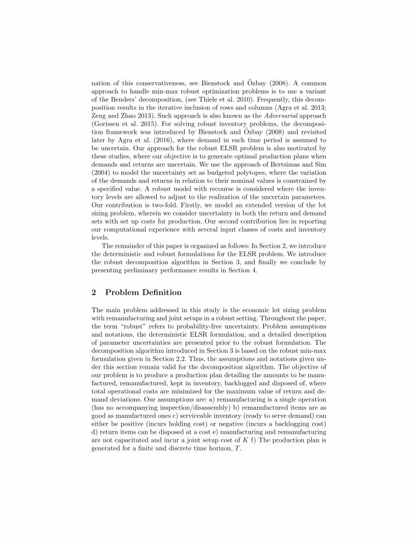
nation of this conservativeness, see Bienstock and Ozbay (2008). A commonapproach to handle min-max robust optimization problems is to use a variantof the Benders’ decomposition, (see Thiele et al. 2010). Frequently, this decom-position results in the iterative inclusion of rows and columns (Agra et al. 2013;Zeng and Zhao 2013). Such approach is also known as the Adversarial approach(Gorissen et al. 2015). For solving robust inventory problems, the decomposi-tion framework was introduced by Bienstock and Ozbay (2008) and revisitedlater by Agra et al. (2016), where demand in each time period is assumed tobe uncertain. Our approach for the robust ELSR problem is also motivated bythese studies, where our objective is to generate optimal production plans whendemands and returns are uncertain. We use the approach of Bertsimas and Sim(2004) to model the uncertainty set as budgeted polytopes, where the variationof the demands and returns in relation to their nominal values is constrained bya specified value. A robust model with recourse is considered where the inven-tory levels are allowed to adjust to the realization of the uncertain parameters.Our contribution is two-fold. Firstly, we model an extended version of the lotsizing problem, wherein we consider uncertainty in both the return and demandsets with set up costs for production. Our second contribution lies in reportingour computational experience with several input classes of costs and inventorylevels.

The remainder of this paper is organized as follows: In Section 2, we introducethe deterministic and robust formulations for the ELSR problem. We introducethe robust decomposition algorithm in Section 3, and finally we conclude bypresenting preliminary performance results in Section 4.

2 Problem Definition

The main problem addressed in this study is the economic lot sizing problemwith remanufacturing and joint setups in a robust setting. Throughout the paper,the term “robust” refers to probability-free uncertainty. Problem assumptionsand notations, the deterministic ELSR formulation, and a detailed descriptionof parameter uncertainties are presented prior to the robust formulation. Thedecomposition algorithm introduced in Section 3 is based on the robust min-maxformulation given in Section 2.2. Thus, the assumptions and notations given un-der this section remain valid for the decomposition algorithm. The objective ofour problem is to produce a production plan detailing the amounts to be manu-factured, remanufactured, kept in inventory, backlogged and disposed of, wheretotal operational costs are minimized for the maximum value of return and de-mand deviations. Our assumptions are: a) remanufacturing is a single operation(has no accompanying inspection/disassembly) b) remanufactured items are asgood as manufactured ones c) serviceable inventory (ready to serve demand) caneither be positive (incurs holding cost) or negative (incurs a backlogging cost)d) return items can be disposed at a cost e) manufacturing and remanufacturingare not capacitated and incur a joint setup cost of K f) The production plan isgenerated for a finite and discrete time horizon, T .

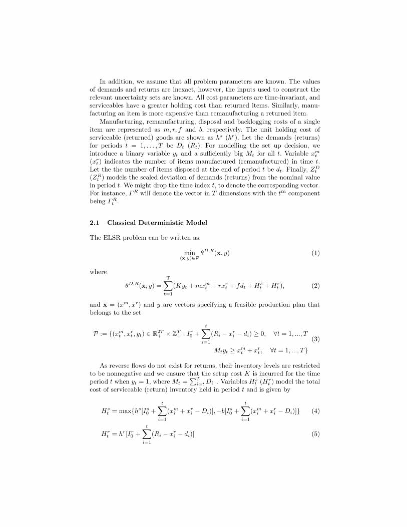
In addition, we assume that all problem parameters are known. The valuesof demands and returns are inexact, however, the inputs used to construct therelevant uncertainty sets are known. All cost parameters are time-invariant, andserviceables have a greater holding cost than returned items. Similarly, manu-facturing an item is more expensive than remanufacturing a returned item.

Manufacturing, remanufacturing, disposal and backlogging costs of a singleitem are represented as m, r, f and b, respectively. The unit holding cost ofserviceable (returned) goods are shown as hs (hr). Let the demands (returns)for periods t = 1, . . . , T be Dt (Rt). For modelling the set up decision, weintroduce a binary variable yt and a sufficiently big Mt for all t. Variable xmt(xrt ) indicates the number of items manufactured (remanufactured) in time t.Let the the number of items disposed at the end of period t be dt. Finally, ZDt(ZRt ) models the scaled deviation of demands (returns) from the nominal valuein period t. We might drop the time index t, to denote the corresponding vector.For instance, ΓR will denote the vector in T dimensions with the tth componentbeing ΓRt .

2.1 Classical Deterministic Model

The ELSR problem can be written as:

min(x,y)∈P

θD,R(x, y) (1)

where

θD,R(x, y) =

T∑t=1

(Kyt +mxmt + rxrt + fdt +Hst +Hr

t ), (2)

and x = (xm, xr) and y are vectors specifying a feasible production plan thatbelongs to the set

P := {(xmt , xrt , yt) ∈ R2T+ × ZT+ : Ir0 +

t∑i=1

(Ri − xri − di) ≥ 0, ∀t = 1, ..., T

Mtyt ≥ xmt + xrt , ∀t = 1, ..., T}

(3)

As reverse flows do not exist for returns, their inventory levels are restrictedto be nonnegative and we ensure that the setup cost K is incurred for the timeperiod t when yt = 1, where Mt =

∑Ti=tDi . Variables Hs

t (Hrt ) model the total

cost of serviceable (return) inventory held in period t and is given by

Hst = max{hs[Is0 +

t∑i=1

(xmi + xri −Di)],−b[Is0 +

t∑i=1

(xmi + xri −Di)]} (4)

Hrt = hr[Ir0 +

t∑i=1

(Ri − xri − di)] (5)

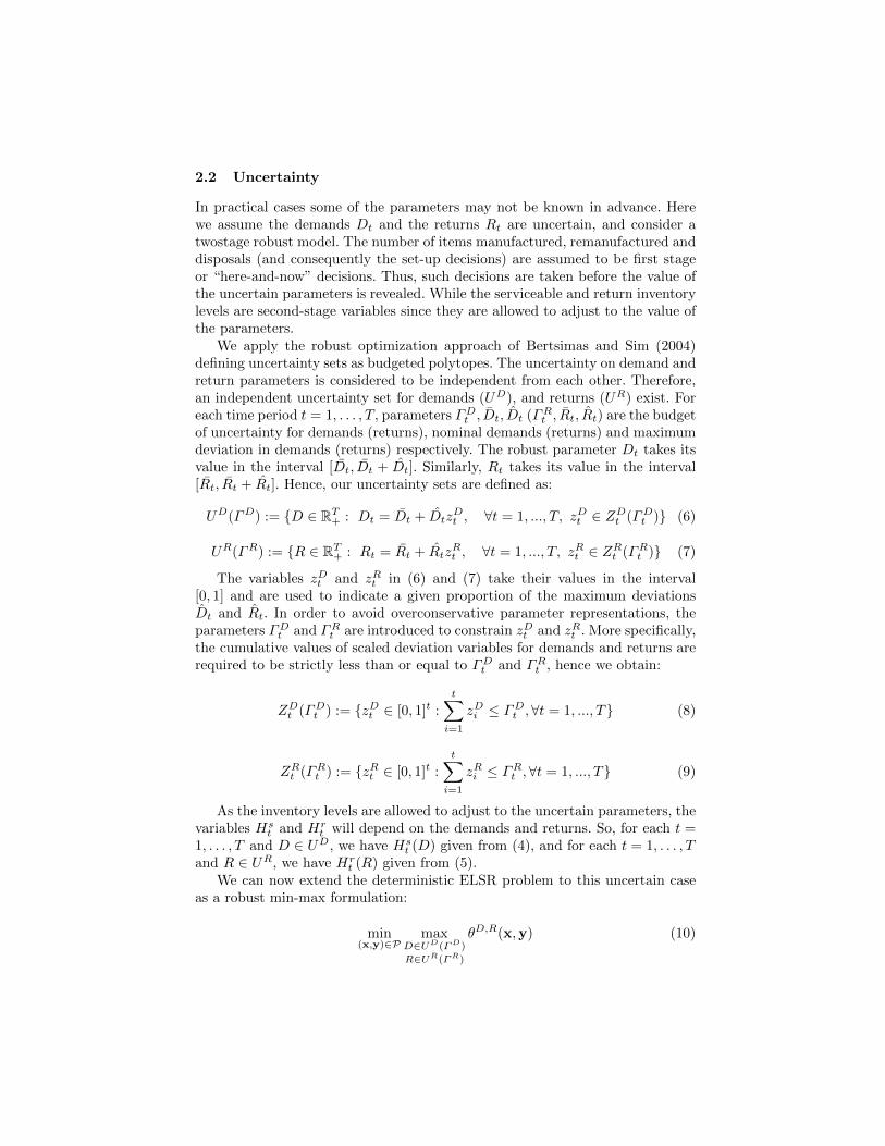
2.2 Uncertainty

In practical cases some of the parameters may not be known in advance. Herewe assume the demands Dt and the returns Rt are uncertain, and consider atwostage robust model. The number of items manufactured, remanufactured anddisposals (and consequently the set-up decisions) are assumed to be first stageor “here-and-now” decisions. Thus, such decisions are taken before the value ofthe uncertain parameters is revealed. While the serviceable and return inventorylevels are second-stage variables since they are allowed to adjust to the value ofthe parameters.

We apply the robust optimization approach of Bertsimas and Sim (2004)defining uncertainty sets as budgeted polytopes. The uncertainty on demand andreturn parameters is considered to be independent from each other. Therefore,an independent uncertainty set for demands (UD), and returns (UR) exist. Foreach time period t = 1, . . . , T, parameters ΓDt , Dt, Dt (ΓRt , Rt, Rt) are the budgetof uncertainty for demands (returns), nominal demands (returns) and maximumdeviation in demands (returns) respectively. The robust parameter Dt takes itsvalue in the interval [Dt, Dt + Dt]. Similarly, Rt takes its value in the interval[Rt, Rt + Rt]. Hence, our uncertainty sets are defined as:

UD(ΓD) := {D ∈ RT+ : Dt = Dt + DtzDt , ∀t = 1, ..., T, zDt ∈ ZDt (ΓDt )} (6)

UR(ΓR) := {R ∈ RT+ : Rt = Rt + RtzRt , ∀t = 1, ..., T, zRt ∈ ZRt (ΓRt )} (7)

The variables zDt and zRt in (6) and (7) take their values in the interval[0, 1] and are used to indicate a given proportion of the maximum deviationsDt and Rt. In order to avoid overconservative parameter representations, theparameters ΓDt and ΓRt are introduced to constrain zDt and zRt . More specifically,the cumulative values of scaled deviation variables for demands and returns arerequired to be strictly less than or equal to ΓDt and ΓRt , hence we obtain:

ZDt (ΓDt ) := {zDt ∈ [0, 1]t :

t∑i=1

zDi ≤ ΓDt ,∀t = 1, ..., T} (8)

ZRt (ΓRt ) := {zRt ∈ [0, 1]t :

t∑i=1

zRi ≤ ΓRt ,∀t = 1, ..., T} (9)

As the inventory levels are allowed to adjust to the uncertain parameters, thevariables Hs

t and Hrt will depend on the demands and returns. So, for each t =

1, . . . , T and D ∈ UD, we have Hst (D) given from (4), and for each t = 1, . . . , T

and R ∈ UR, we have Hrt (R) given from (5).

We can now extend the deterministic ELSR problem to this uncertain caseas a robust min-max formulation:

min(x,y)∈P

maxD∈UD(ΓD)

R∈UR(ΓR)

θD,R(x,y) (10)

where θD,R(x, y) is extended as follows:

θD,R(x, y) =

T∑t=1

(Kyt +mxmt + rxrt + fdt +Hst (D) +Hr

t (R)) (11)

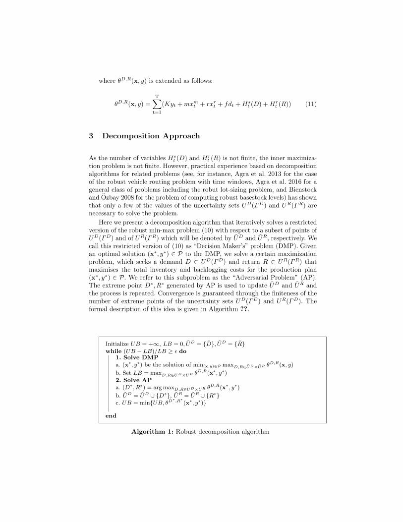
3 Decomposition Approach

As the number of variables Hst (D) and Hr

t (R) is not finite, the inner maximiza-tion problem is not finite. However, practical experience based on decompositionalgorithms for related problems (see, for instance, Agra et al. 2013 for the caseof the robust vehicle routing problem with time windows, Agra et al. 2016 for ageneral class of problems including the robut lot-sizing problem, and Bienstockand Ozbay 2008 for the problem of computing robust basestock levels) has shownthat only a few of the values of the uncertainty sets UD(ΓD) and UR(ΓR) arenecessary to solve the problem.

Here we present a decomposition algorithm that iteratively solves a restrictedversion of the robust min-max problem (10) with respect to a subset of points ofUD(ΓD) and of UR(ΓR) which will be denoted by UD and UR, respectively. Wecall this restricted version of (10) as “Decision Maker’s” problem (DMP). Givenan optimal solution (x∗, y∗) ∈ P to the DMP, we solve a certain maximizationproblem, which seeks a demand D ∈ UD(ΓD) and return R ∈ UR(ΓR) thatmaximises the total inventory and backlogging costs for the production plan(x∗, y∗) ∈ P. We refer to this subproblem as the “Adversarial Problem” (AP).The extreme point D∗, R∗ generated by AP is used to update UD and UR andthe process is repeated. Convergence is guaranteed through the finiteness of thenumber of extreme points of the uncertainty sets UD(ΓD) and UR(ΓD). Theformal description of this idea is given in Algorithm ??.

Initialize UB = +∞, LB = 0, UD = {D}, UD = {R}while (UB − LB)/LB ≥ ε do

1. Solve DMPa. (x∗, y∗) be the solution of min(x,y)∈P maxD,R∈UD×UR θ

D,R(x, y)

b. Set LB = maxD,R∈UD×UR θD,R(x∗, y∗)

2. Solve APa. (D∗, R∗) = arg maxD,R∈UD×UR θD,R(x∗, y∗)

b. UD = UD ∪ {D∗}, UR = UR ∪ {R∗}c. UB = min{UB, θD

∗,R∗(x∗, y∗)}

end

Algorithm 1: Robust decomposition algorithm

For the sake of completeness, we give the DMP and the AP. In order to modelthe DMP, notice that the inner maximization problem in (10) defined for therestricted set UD × UR, maxD,R∈UD×UR θD,R(x,y), can be written as:

T∑t=1

(Kyt +mxmt + rxrt + fdt) + maxD,R∈UD×UR

T∑t=1

(Hst (D) +Hr

t (R))). (12)

Introducing variable π to indicate the maximum value of the total inventoryand backlogging costs over all possible realizations of demands and returns, theDMP can be written as follows:

min

T∑t=1

(Kyt +mxmt + rxrt + fdt) + π (13)

s.t. π ≥T∑

t=1

(Hst (D) +Hr

t (R)) ∀D ∈ UD∀R ∈ UR

(14)

Hst (D) ≥ hs

(Is0 +

t∑i=1

(xmi + xri −Di)) ∀t = 1, ..., T

∀D ∈ UD(15)

Hst (D) ≥ −b

(Is0 +

t∑i=1

(xmi + xri −Di))) ∀t = 1, ..., T

∀D ∈ UD(16)

Hrt (R) = hr

(Ir0 +

t∑i=1

(Ri − xri − di)),

∀t = 1, ..., T∀R ∈ UR

(17)

t∑i=1

(Ri − di − xri ) ≥ 0∀t = 1, ..., T∀R ∈ UR

(18)

Mtyt ≥ xmt + xrt ∀t = 1, ..., T (19)

(x, y) ∈ P

Note that variables Hrt (R) can be eliminated using equations (17). Given a

solution for variables xmi , xri , di, the AP is formulated as follows:

max π (20)

s.t. π ≤T∑

t=1

(Hst + hr

t∑i=1

(Ri + RizRi − di − xri )) (21)

Hst = max

{hs(Is0 +

t∑i=1

(xmi + xri − (Di + DizDi )),

− b(Is0 +

t∑i=1

(xmi + xri − (Di + DizDi ))}

∀t = 1, ..., T (22)

Ir0 +

t∑i=1

(Ri + RizRi − xri − di) ≥ 0 ∀t = 1, ..., T (23)

t∑i=1

zDi ≤ ΓDt ,

t∑i=1

zRi ≤ ΓRt ∀t = 1, ..., T (24)

0 ≤ zDjt ≤ 1, 0 ≤ zRj

t ≤ 1 ∀t = 1, ..., T (25)

In order to linearize (22), we introduce binary variable st indicating whetherinventory is kept or demand is backlogged, and rewrite it as:

Hst ≤ hs

(Is0 +

t∑i=1

(xmi + xri − (Di + DizDi ))

+M1t(1− st) ∀t = 1, ..., T (26)

Hst ≤ −b

(Is0 +

t∑i=1

(xmi + xri − (Di + DizDi ))

+M2tst ∀t = 1, ..., T (27)

4 Experiments

The proposed decomposition algorithm was implemented in Java using EclipseMars. Our formulations were implemented and solved as MIPs using Java API forCPLEX 12.6 on an Intel Core i5, 3.30GHz CPU, 3.29GHz, 8 GB RAM machine.

Additionally, each run has been restricted to a total running time of 10,000seconds. The terminating condition for instances with a smaller running time isset as ε = 0.01, where ε = UB−LB

LB .

4.1 Data Generation

Data sets have been generated for different levels of four parameter types: num-ber of returns, probability of constraint violation caused by ΓDt and ΓRt , thesetup cost and the disposal cost. We consider three different levels for eachgroup, except for disposal costs: low, medium and high. For disposal costs, weare interested in observing two different cases, namely when the disposal cost is

greater or less than the remanufacturing cost. Throughout this section, the datasets are abbreviated as “ABCD T”, where each letter indicates the levels of theaforementioned parameters in their given order, with T time periods.

For all data sets, nominal demand is generated randomly in the interval[50, 100]. Likewise, returns are generated randomly in intervals [15, 30], [25, 50]and [35, 70], for low, medium and high levels, respectively. Maximum demandand return deviations are calculated as Dt = 0.1Dt and Rt = 0.1Rt . In order todetermine ΓDt and ΓRt , we use the probabilistic bounds given by Bertsimas andSim (2004). We set the probability of constraint violation as 0.01, 0.05 and 0.10,for low, medium and high levels, respectively. To determine the setup cost, weuse the following equations: K = 0.1Dminh

s, K = 2Dmedhs and K = 5Dmaxh

s,where Dmin = 50, Dmed = 75 and Dmax = 100, for low, medium and highlevels. Finally, the disposal cost is set as d = 0.5r when it is less than theremanufacturing cost, and as d = 2r otherwise.

In addition, the holding cost of serviceables is generated in the interval [5, 10],through which the remaining cost parameters are defined. We set the holding costfor returns as hr = 0.1hs, the backlogging cost as b = 4hs, the manufacturingcost as m = 2hr, and the remanufacturing cost as r = 2hr .

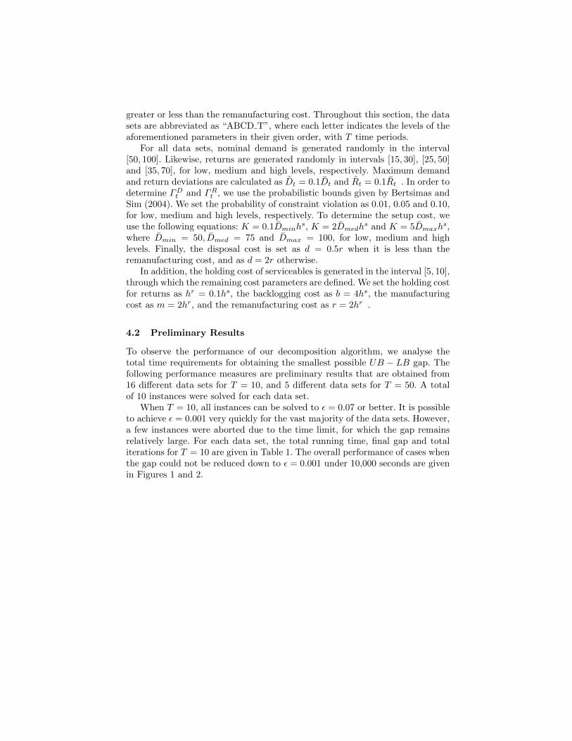
4.2 Preliminary Results

To observe the performance of our decomposition algorithm, we analyse thetotal time requirements for obtaining the smallest possible UB − LB gap. Thefollowing performance measures are preliminary results that are obtained from16 different data sets for T = 10, and 5 different data sets for T = 50. A totalof 10 instances were solved for each data set.

When T = 10, all instances can be solved to ε = 0.07 or better. It is possibleto achieve ε = 0.001 very quickly for the vast majority of the data sets. However,a few instances were aborted due to the time limit, for which the gap remainsrelatively large. For each data set, the total running time, final gap and totaliterations for T = 10 are given in Table 1. The overall performance of cases whenthe gap could not be reduced down to ε = 0.001 under 10,000 seconds are givenin Figures 1 and 2.

0

0.01

0.02

0.03

0.04

0.05

0.06

0.07

0.08

HHLG HHLL HMLG HMLL

Gap

Dataset

Fig. 1: Total UB - LB gap for T=10(when gap is greater than 0.01).

0

1000

2000

3000

4000

5000

6000

7000

8000

9000

10000

HHLG HHLL HMLG HMLL HLLG HHML HLLL

To

tal

tim

e ta

ken

(s)

Dataset

Fig. 2: Total running time for T=10(when ε > 0.01 could not be achievedunder 10,000 seconds).

Table 1: Gap, time, iteration performance for T=10.

Gap (ε) Time Performance (s) Number of Iterations

Dataset Avg. Std.Dev. Avg. Std.Dev. Avg. Std.Dev.

HHHG 0.004 0.002 0.4 0.1 4.2 0.9HHHL 0.003 0.003 0.7 0.3 4.9 1.1HHMG 0.005 0.003 27.8 40.5 5.9 1.2HHML 0.003 0.002 236.2 692.5 5.3 0.9HHLG 0.020 0.021 1706.0 2314.5 4.2 1.5HHLL 0.018 0.022 6783.9 4337.9 4.2 1.2HMHG 0.004 0.004 0.4 0.2 3.7 0.9HMHL 0.005 0.004 0.3 0.2 3.9 0.3HMLG 0.007 0.008 5247.2 4542.0 4.6 1.0HMLL 0.008 0.013 4713.2 4512.3 4.5 1.2HLHG 0.007 0.004 0.3 0.1 2.8 0.4HLHL 0.005 0.004 0.4 0.2 3.0 0.5HLMG 0.005 0.003 32.7 54.7 3.8 0.4HLML 0.004 0.005 19.8 34.1 3.9 0.6HLLG 0.002 0.004 401.4 617.4 4.2 0.6HLLL 0.002 0.003 433.5 1024.5 4.2 0.8

As the detailed results in Table 1 indicate, the gaps achieved and number ofiterations needed are in general consistent across different data sets, in additionto being in general very small (e.g., the highest maximum gap is still under 0.1,and no more than 8 iterations were necessary for any instance). On the otherhand, as it can be also observed from the Figures 1 and 2, the time performancecan vary significantly not only among different datasets but also among differentinstances of most datasets.

When we look into the datasets with T = 50, a greater number of instancesnaturally run until the maximum time limit is reached as a consequence of theincreased number of periods. However, the algorithm is still able to close the gapup to ε = 0.003 for some instances.

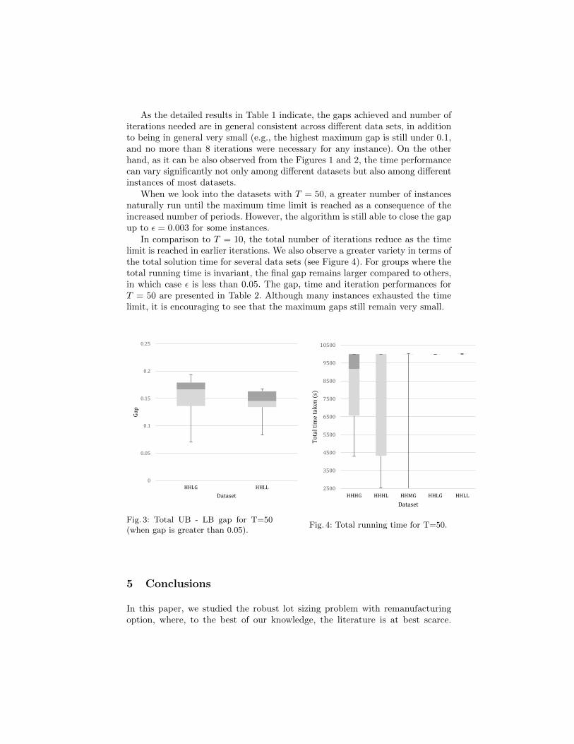
In comparison to T = 10, the total number of iterations reduce as the timelimit is reached in earlier iterations. We also observe a greater variety in terms ofthe total solution time for several data sets (see Figure 4). For groups where thetotal running time is invariant, the final gap remains larger compared to others,in which case ε is less than 0.05. The gap, time and iteration performances forT = 50 are presented in Table 2. Although many instances exhausted the timelimit, it is encouraging to see that the maximum gaps still remain very small.

0

0.05

0.1

0.15

0.2

0.25

HHLG HHLL

Gap

Dataset

Fig. 3: Total UB - LB gap for T=50(when gap is greater than 0.05).

2500

3500

4500

5500

6500

7500

8500

9500

10500

HHHG HHHL HHMG HHLG HHLL

To

tal

tim

e ta

ken

(s)

Dataset

Fig. 4: Total running time for T=50.

5 Conclusions

In this paper, we studied the robust lot sizing problem with remanufacturingoption, where, to the best of our knowledge, the literature is at best scarce.

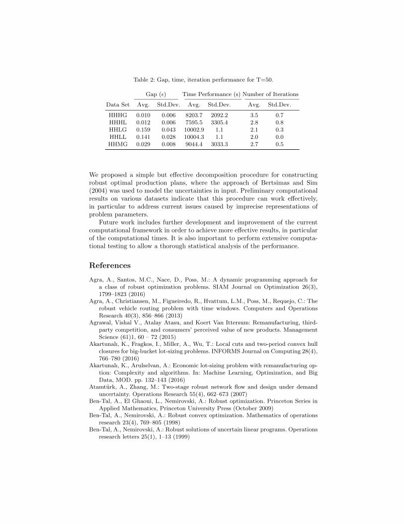
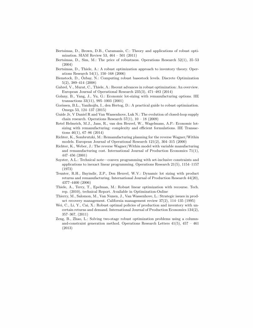
Table 2: Gap, time, iteration performance for T=50.

Gap (ε) Time Performance (s) Number of Iterations

Data Set Avg. Std.Dev. Avg. Std.Dev. Avg. Std.Dev.

HHHG 0.010 0.006 8203.7 2092.2 3.5 0.7HHHL 0.012 0.006 7595.5 3305.4 2.8 0.8HHLG 0.159 0.043 10002.9 1.1 2.1 0.3HHLL 0.141 0.028 10004.3 1.1 2.0 0.0HHMG 0.029 0.008 9044.4 3033.3 2.7 0.5

We proposed a simple but effective decomposition procedure for constructingrobust optimal production plans, where the approach of Bertsimas and Sim(2004) was used to model the uncertainties in input. Preliminary computationalresults on various datasets indicate that this procedure can work effectively,in particular to address current issues caused by imprecise representations ofproblem parameters.

Future work includes further development and improvement of the currentcomputational framework in order to achieve more effective results, in particularof the computational times. It is also important to perform extensive computa-tional testing to allow a thorough statistical analysis of the performance.

References

Agra, A., Santos, M.C., Nace, D., Poss, M.: A dynamic programming approach fora class of robust optimization problems. SIAM Journal on Optimization 26(3),1799–1823 (2016)

Agra, A., Christiansen, M., Figueiredo, R., Hvattum, L.M., Poss, M., Requejo, C.: Therobust vehicle routing problem with time windows. Computers and OperationsResearch 40(3), 856–866 (2013)

Agrawal, Vishal V., Atalay Atasu, and Koert Van Ittersum: Remanufacturing, third-party competition, and consumers’ perceived value of new products. ManagementScience (61)1, 60 – 72 (2015)

Akartunalı, K., Fragkos, I., Miller, A., Wu, T.: Local cuts and two-period convex hullclosures for big-bucket lot-sizing problems. INFORMS Journal on Computing 28(4),766–780 (2016)

Akartunalı, K., Arulselvan, A.: Economic lot-sizing problem with remanufacturing op-tion: Complexity and algorithms. In: Machine Learning, Optimization, and BigData, MOD. pp. 132–143 (2016)

Atamturk, A., Zhang, M.: Two-stage robust network flow and design under demanduncertainty. Operations Research 55(4), 662–673 (2007)

Ben-Tal, A., El Ghaoui, L., Nemirovski, A.: Robust optimization. Princeton Series inApplied Mathematics, Princeton University Press (October 2009)

Ben-Tal, A., Nemirovski, A.: Robust convex optimization. Mathematics of operationsresearch 23(4), 769–805 (1998)

Ben-Tal, A., Nemirovski, A.: Robust solutions of uncertain linear programs. Operationsresearch letters 25(1), 1–13 (1999)

Bertsimas, D., Brown, D.B., Caramanis, C.: Theory and applications of robust opti-mization. SIAM Review 53, 464 – 501 (2011)

Bertsimas, D., Sim, M.: The price of robustness. Operations Research 52(1), 35–53(2004)

Bertsimas, D., Thiele, A.: A robust optimization approach to inventory theory. Oper-ations Research 54(1), 150–168 (2006)

Bienstock, D., Ozbay, N.: Computing robust basestock levels. Discrete Optimization5(2), 389–414 (2008)

Gabrel, V., Murat, C., Thiele, A.: Recent advances in robust optimization: An overview.European Journal of Operational Research 235(3), 471–483 (2014)

Golany, B., Yang, J., Yu, G.: Economic lot-sizing with remanufacturing options. IIEtransactions 33(11), 995–1003 (2001)

Gorissen, B.L., Yanikoglu, I., den Hertog, D.: A practical guide to robust optimization.Omega 53, 124–137 (2015)

Guide Jr, V Daniel R and Van Wassenhove, Luk N.: The evolution of closed-loop supplychain research. Operations Research 57(1), 10 – 18 (2009)

Retel Helmrich, M.J., Jans, R., van den Heuvel, W., Wagelmans, A.P.: Economic lot-sizing with remanufacturing: complexity and efficient formulations. IIE Transac-tions 46(1), 67–86 (2014)

Richter, K., Sombrutzki, M.: Remanufacturing planning for the reverse Wagner/Withinmodels. European Journal of Operational Research 121(2), 304–315 (2000)

Richter, K., Weber, J.: The reverse Wagner/Within model with variable manufacturingand remanufacturing cost. International Journal of Production Economics 71(1),447–456 (2001)

Soyster, A.L.: Technical note—convex programming with set-inclusive constraints andapplications to inexact linear programming. Operations Research 21(5), 1154–1157(1973)

Teunter, R.H., Bayindir, Z.P., Den Heuvel, W.V.: Dynamic lot sizing with productreturns and remanufacturing. International Journal of Production Research 44(20),4377–4400 (2006)

Thiele, A., Terry, T., Epelman, M.: Robust linear optimization with recourse. Tech.rep. (2010), technical Report. Available in Optimization-Online

Thierry, M., Salomon, M., Van Nunen, J., Van Wassenhove, L.: Strategic issues in prod-uct recovery management. California management review 37(2), 114–135 (1995)

Wei, C., Li, Y., Cai, X.: Robust optimal policies of production and inventory with un-certain returns and demand. International Journal of Production Economics 134(2),357–367, (2011)

Zeng, B., Zhao, L.: Solving two-stage robust optimization problems using a column-and-constraint generation method. Operations Research Letters 41(5), 457 – 461(2013)