Embed Size (px)
Citation preview
Road Condition Based Adaptive Model Predictive Control for Autonomous Vehicles
Xin Wang School of Construction Machinery
Chang’an University Xi’an, Shaanxi 710064, China
Department of Automotive Engineering
Clemson University Greenville, SC 29607, USA
Longxiang Guo Department of Automotive
Engineering Clemson University
Greenville, SC 29607, USA [email protected]
Yunyi Jia* Department of Automotive
Engineering Clemson University
Greenville, SC 29607, USA [email protected]
ABSTRACT
Road conditions are of critical importance for motion
control problems of the autonomous vehicle. In the existing
studies of Model Predictive Control (MPC), road condition is
generally modeled with the system dynamics, sometimes
simplified as common disturbances, or even ignored based on
some assumptions. For most of such MPC formulations, the
cost function is usually designed as fixed function and has no
relations with the time-varying road conditions. In order to
comprehensively deal with the uncertain road conditions and
improve the overall control performance, a new model
predictive control strategy based on a mechanism of adaptive
cost function is proposed in this paper. The relation between the
cost function and road conditions is established based on a set
of priority policies which reflect the different cost requirements
under different road grades and friction coefficients. The
adaptive MPC strategy is applied to solve the longitudinal
control problem of autonomous vehicles. Simulation studies are
conducted on the MPC method with both the fixed cost
function and the adaptive cost function. The results show that
the proposed adaptive MPC approach can achieve a better
overall control performance under different road conditions.
Keywords
Model Predictive Control, Longitudinal control, Adaptive cost
function, Road condition.
1 INTRODUCTION
With the rapid development of autonomous driving
technology, many basic self-driving functions have been
implemented and applied to autonomous vehicles successfully.
*Corresponding Author, [email protected]
The latest autonomous vehicles have the functions of adaptive
cruise control, lane keeping, autonomous parking and crash
avoidance, etc., due to the applications of various control
methods and other information techniques. Many people
believe that autonomous vehicles will replace traditional
vehicles gradually and become a major transportation tool
someday in the future [1]. Nowadays, people are no longer
satisfied with merely the safety and the basic functions of the
autonomous vehicle. Higher demands are placed on the
driving/riding comfort and control efficiency. Hence, more
sophisticated control strategies and methods are expected to
improve the control performance with lower control costs.
In recent years, Model Predictive Control (MPC) method
has gained much attention in the field of autonomous vehicles,
due to its unique advantages in solving control problems that
are hard to model accurately and/or have constraints [2]. In
most of the autonomous driving problems, system constraints
are inevitable. These constraints include mechanical input
limitations, the acceleration ability and the safe distance
between the vehicle and other objects, etc. Naturally, MPC
becomes an ideal choice to solve such problems.
In motion control problems of the autonomous vehicle,
road condition is an ineligible factor which influences the
control performance significantly. For moving vehicles, road
conditions mainly refer to the road grade and the friction
coefficient. The former is primarily decided by the
physiographic condition and the design of the road, while the
latter is subject to many factors, including the road pavement
material, the age of the road, and even the weather [3]. Since
road conditions are time-varying and uncertain, comprehensive
modeling is difficult to realize. Therefore, it is meaningful to
deal with the road condition by other ways.
In the existing MPC studies of autonomous vehicles, road
conditions are considered more or less. In most cases, the road
Proceedings of the ASME 2018Dynamic Systems and Control Conference
DSCC2018September 30-October 3, 2018, Atlanta, Georgia, USA
DSCC2018-9095
1 Copyright © 2018 ASME
Attendee R
ead-Only C
opy

condition, especially the friction coefficient, is modeled with
the system dynamics, as parameters or disturbances. Borrelli et
al. in [4] applied nonlinear MPC to the autonomous steering
system. In their study, the bicycle model and the road-tire
model of the vehicle are combined to establish the system
dynamics. The road friction coefficient is considered as a
parameter of the system dynamics. Falcone et al. in [5] and [6]
also studied the active steering problem based on the same
system dynamics as [4], but using a successive online
linearization approach. In [7], Turri et al. studied the lane
keeping and obstacle avoidance problems based on linear MPC.
The extended bicycle mode is utilized and the friction
coefficient is modeled with the longitudinal tire force. Carvalho
et al. in [8] presented their design of a nonlinear MPC
controller, which can track the lane centerline while avoiding
collisions with obstacles. In their study, the friction coefficient
is also incorporated in the longitudinal tire force model. In [9],
Kamal et al. introduced an energy-saving MPC strategy and
applied it to the adaptive cruise control problem. A concept of
equivalent acceleration is proposed considering the effect of the
road grade. In some other MPC studies, road conditions are
treated as the system constraints. Yi et al. in [10] studied the
MPC-based trajectory planning for critical driving maneuvers.
They introduced a quadratic MPC control method considering
friction limits in evasion maneuvers. In [11], Jalalmaab et al.
proposed an MPC-based collision avoidance scheme for
autonomous vehicles. The maximum road friction coefficient is
considered in the acceleration constraints, and a particular
optimization method is developed to estimate the max road
friction coefficient. In [12], Beal et al. presented a vehicle
stabilization approach by utilizing a model predictive envelope
controller to bound the vehicle motion within the stable region
of the state space. The estimated road condition is used to
define the state boundaries. Among the above studies, the factor
of road grade is not mentioned in [4-8,10-12], while in [9], the
road friction coefficient is not taken into account.
Due to the difficulty of being detected, the information of
road conditions is always obtained through model-based
estimation techniques in many applications. Chen et al. in [13]
designed a recursive least square estimator to achieve the road
friction coefficient online. Kidambi, et al. in [14], developed a
mass and grade estimation method using longitudinal
acceleration. Similar studies can also be found in [15-19].
Whereas, in some of the MPC studies, due to the complexity of
the system, road conditions are not taken into account in the
control process, as in [20-21].
In spite of these existing studies, research and applications
regarding adaptive cost function strategies have rarely been
addressed. In most of the existing MPC studies, road conditions
are usually simplified based on some assumptions, and not all
the factors are modeled with system dynamics. Meanwhile, in
these MPC studies, traditional cost functions with fixed penalty
weights are used, and there is no special design for the cost
function. Therefore, the main contribution of this paper is the
development of a new MPC strategy with the adaptive cost
function in the receding optimization process based on the
time-varying road conditions. This approach keeps all the
advantages of MPC method and at the same time considers the
different requirements of the optimization objectives under
different road conditions. By using the proposed approach, the
control performance can be accomplished with a much lower
control cost.
The remainder of this paper is organized as follows:
Section II describes the control problem to be studied, and
formulates the system dynamics. The MPC controller is
designed and solved in Section III. In Section IV, the road
condition adaptive strategy is devised. Simulation study is
presented and discussed in Section V. Finally, conclusions and
future work of this paper are addressed in Section VI.
2 PROBLEM FORMULATION
The purpose of this paper is to investigate a new road
condition adaptive MPC strategy. To achieve this goal, the
longitudinal control problem is chosen as a preliminary study,
because it is less complicated than other motion control
problems. For the same reason, a mass point model is utilized
to describe the system dynamics.
In the longitudinal control problem, the actual velocity 𝑣
of the vehicle must well track the given reference velocity 𝑣𝑟 .
An MPC controller will be designed to implement this control
with consideration of the time-varying road conditions.
Figure 1. Force diagram of a moving vehicle on the upgrade road
Both the road grade and the friction coefficient are
considered in the control process. We use 𝜃 to represent the
road grade, as shown in Figure 1, which can be detected via the
attitude sensor equipped in the vehicle. The friction coefficient,
which has strong stochastic characteristics, is hard to detect by
existing sensors. Therefore, the slip ratio is employed to replace
the friction coefficient approximately in this study, which is
defined by
𝑠 = 1 − 𝑣𝑅𝜔 {𝑣 ≠ 0 for braking𝜔 ≠ 0 for driving (1)
where s is the slip ratio; 𝜔 is the angular speed of the vehicle
wheel; 𝑅 is the tire radius.
As shown in Figure 1, the autonomous vehicle is regarded
as a mass point in the longitudinal control problem. We can
establish its dynamic model by using Newton’s Second Law
directly [22, 23], and thus have
𝑚�̇� = 𝑚𝑢 − 12 𝐶𝑑𝜌𝑎𝐴𝑓𝑣2 − 𝐶𝑟𝛽(𝑠)𝑚𝑔cos(𝜃) − 𝑚𝑔sin(𝜃) (2)
where 𝑣 is the velocity of the vehicle; 𝑢 is the acceleration
control input per unit mass to accelerate or decelerate the car
which is derived from the control strategy; 𝑚 is the vehicle
mass; 𝜌𝑎 is the air density; 𝐶𝑑 is the drag coefficient; 𝐴𝑓 is
2 Copyright © 2018 ASME

the frontal area of the vehicle; 𝐶𝑟 is the rolling resistance
coefficient; 𝛽 is an influence factor which is related to the road
friction coefficient/slip ratio 𝑠.
In general, the system dynamics of a vehicle is always
non-linear. For the reason that a non-linear MPC problem is
harder to solve than a linear MPC problem, we can simplify the
non-linear model to a linear one. By linearization and
discretization, a linear CARIMA model can be obtained.
CARIMA model is the most common used transfer function
model in MPC [24]. It is a discrete and one-step-ahead
prediction model, and can be expressed by
𝑎(𝑧)𝑦𝑘 = 𝑏(𝑧)𝑢𝑘 + 𝑤𝑘𝛥 (3)
where 𝑢𝑘 , 𝑦𝑘 and 𝑤𝑘 are the sampled values of the input 𝑢(𝑡), the output 𝑦(𝑡) and the system disturbance 𝑤(𝑡) at
time instant 𝑘 , respectively; 𝑎(𝑧) and 𝑏(𝑧) are the
denominator and the numerator polynomial of the impulse
response transfer function of the system, which can be derived
from model (2) by using z Transform; 𝛥 is the sampling time
interval. Then (3) can be written as
𝐴(𝑧)𝑦𝑘 = 𝑏(𝑧)𝛥𝑢𝑘 + 𝑤𝑘 (4)
where 𝐴(𝑧) = 𝑎(𝑧)𝛥 = 1 + 𝐴1𝑧−1 + ⋯+ 𝐴𝑛𝑧−𝑛 , and 𝑏(z) = 𝑏1𝑧−1 + ⋯ + 𝑏𝑚𝑧−𝑚 , where 𝑛 and 𝑚 are the order
and the input number of the system, respectively. Consequently,
the discrete model of the system can be represented by
𝑦𝑘+1 + 𝐴1𝑦𝑘 + ⋯+ 𝐴𝑛𝑦𝑘−𝑛+1 = 𝑏1Δ𝑢𝑘 + 𝑏2Δ𝑢𝑘−1 + ⋯+𝑏𝑚Δ𝑢𝑘−𝑚+1 (5)
where Δ𝑢𝑘 is the input increment. The output 𝑦𝑘 is often
measurable in practice. Equation (5) is the basis of the
one-step-ahead prediction, which can be used recursively to get
an n-step-ahead prediction.
3 MPC CONTROLLER DESIGN
To get the solution of the control, the linear MPC problem
can be converted to a standard QP (Quadratic Programming)
problem, as shown by (6).
{min𝑥 𝐽 = 𝑥𝑇𝑆𝑥 + 𝑥𝑇𝑓 + 𝑐𝑠. 𝑡. 𝑀𝑥 ≤ 𝑑 (6)
where 𝑆 is the weight matrix; 𝑓 and 𝑐 are the coefficient
matrix of the first-order term, and the constant matrix,
respectively; 𝑀 and 𝑑 are the coefficient matrix and the
border matrix of the inequality constraint, respectively.
By minimizing the cost function 𝐽 the optimal solution 𝑥𝑜𝑝𝑡 can be achieved under the system constraints.
3.1 Output Prediction
Referring to [24], we can express the multi-step output
prediction as
�⃗�𝑘+1 = 𝐻∆�⃗⃗�𝑘 + 𝑃∆�⃖⃗�𝑘−1 − 𝑄�⃖�𝑘 (7)
where the notation “” represents “future”, and “” represents “past” in the prediction; 𝐻 = 𝐶𝐴−1𝐶𝑏 , 𝑃 = 𝐶𝐴−1𝐻𝑏
and 𝑄 = 𝐶𝐴−1𝐻𝐴, with the parameter matrices 𝐶𝐴, 𝐶𝑏, 𝐻𝐴 and 𝐻𝑏 defined as
𝐶𝐴 = [ 1 0 0 ⋯ 0𝐴1 1 0 ⋯ 0𝐴2 𝐴1 1 ⋯ ⋮ ⋮ ⋮ ⋮ ⋮ 1𝐴𝑛𝑦 ⋯ 𝐴2 𝐴1 1]
, 𝐶𝑏 = [𝑏1 0𝑏2 𝑏1 0 00 0⋮ ⋮𝑏𝑛𝑢 ⋯ 𝑏1 ⋮𝑏2 𝑏1
],
𝐻𝐴 = [ 𝐴1 ⋯ 𝐴𝑛−𝑛𝑦𝐴2 ⋯ 𝐴𝑛−𝑛𝑦+1 𝐴𝑛−𝑛𝑦+1 ⋯ 𝐴𝑛𝐴𝑛−𝑛𝑦+2 ⋯ 0⋮ ⋮ ⋮ 𝐴𝑛𝑦 ⋯ 𝐴𝑛−1 ⋮ ⋮ ⋮ 𝐴𝑛 ⋯ 0 ]
, and
𝐻𝑏 = [ 𝑏2 ⋯ 𝑏𝑚−𝑛𝑢𝑏3 ⋯ 𝑏𝑚−𝑛𝑢+1 𝑏𝑚−𝑛𝑢+1 ⋯ 𝑏𝑚𝑏𝑚−𝑛𝑢+2 ⋯ 0⋮ ⋮ ⋮ 𝑏𝑛𝑢+1 ⋯ 𝑏𝑚−1 ⋮ ⋮ ⋮ 𝑏𝑚 ⋯ 0 ]
and {�⃗�𝑘+1 = [𝑦𝑘+1 𝑦𝑘+2 … 𝑦𝑘+𝑛𝑦]𝑇 �⃖�𝑘= [𝑦𝑘 𝑦𝑘−1 … 𝑦𝑘−𝑛𝑦+1]𝑇 ∆�⃗⃗�𝑘 = [∆𝑢𝑘 ∆𝑢𝑘+1 … ∆𝑢𝑘+𝑛𝑢−1]𝑇
where 𝑛𝑦 and 𝑛𝑢 are the prediction horizon and the input
horizon, respectively.
3.2 Standardization of the Cost Function
Typically, the cost function acts as the performance index
of an optimization control process. In our problem, the cost
function consists of four penalty terms, including the terms of
vehicle velocity 𝑣, velocity rate ∆𝑣, acceleration control input 𝑢 and its rate ∆𝑢. Among them, ∆𝑣 is relative to the velocity
smoothness, 𝑢 is the control input and ∆𝑢 represents “vehicle
jerking”. We design our cost function 𝐽 based on the four
factors, and it is described as
𝐽 = 𝑊1(𝑣𝑟⃗⃗ ⃗⃗ 𝑘+1 − �⃗�𝑘+1)𝑇(𝑣𝑟⃗⃗ ⃗⃗ 𝑘+1 − �⃗�𝑘+1) +𝑊2�⃗�𝑘+1𝑇 �⃗�𝑘+1 + 𝑊3�⃗⃗�𝑘𝑇 �⃗⃗�𝑘 + 𝑊4∆�⃗⃗�𝑘𝑇∆�⃗⃗�𝑘 (8)
where 𝑊𝑖 (i = 1,2,3,4) are the weights of the four penalty
terms, respectively. Through mathematical deductions, the
optimization objective can be expressed by
min⏟∆�⃗⃗⃗�𝑘 𝐽 =min⏟∆�⃗⃗⃗�𝑘 ∆�⃗⃗�𝑘𝑇 [(𝑊1 + 𝑊2)𝐻𝑇𝐻 + (𝑊3 + 𝑊4)𝐼]∆�⃗⃗�𝑘 +2∆�⃗⃗�𝑘𝑇[(𝑊1 + 𝑊2)𝐻𝑇(𝑃∆�⃖⃗�𝑘−1 + 𝑄�⃖�𝑘) − 𝑊1𝐻𝑇𝑟𝑘+1 +𝑊3∆�⃖⃗�𝑘−1] (9)
Then, we can convert our problem to a standard QP problem as
defined by (6), with 𝑥 = ∆�⃗⃗�𝑘 and
3 Copyright © 2018 ASME
{𝑆 = (𝑊1 + 𝑊2)𝐻𝑇𝐻 + (𝑊3 + 𝑊4)𝐼 𝑓 = 2[(𝑊1 + 𝑊2)𝐻𝑇(𝑃∆�⃗⃖�𝑘−1 + 𝑄�⃖�𝑘) − 𝑊1𝐻𝑇𝑟𝑘+1 + 𝑊3∆�⃗⃖�𝑘−1] 𝑐 = 0
For the space limitation of this paper, the proof of (9) is
omitted here.
3.3 Standardization of the Constraints
In our problem, both the control input 𝑢𝑘 and its rate ∆𝑢𝑘
are physically limited. They are constrained by {𝑢 ≤ 𝑢𝑘 ≤ 𝑢, ∀𝑘 ∆𝑢 ≤ ∆𝑢𝑘 ≤ ∆𝑢, ∀𝑘 (10)
where 𝑢 and 𝑢 are the upper and lower limits of 𝑢𝑘 ,
respectively; ∆𝑢 and ∆𝑢 are the upper and lower limits of ∆𝑢𝑘, respectively. Referring to [25], we can combine the two
constraints by a compact matrix expression as
[𝐶∆𝑢𝐶𝑢𝐸] ∆�⃗⃗�𝑘 ≤ [𝑑∆𝑢𝑑𝑢 ] + [ 0−𝐶𝑢𝐿] 𝑢𝑘−1 (11)
where
𝐶𝑢, 𝐶∆𝑢 =[ 1 0 ⋯ 0 0 1 ⋯ 0 ⋮ ⋮ ⋮ ⋮ 0 0 ⋯ 1−1 0 ⋯ 0 0 −1 ⋯ 0 ⋮ ⋮ ⋮ ⋮ ]
, 𝐸 = [1 01 1 ⋯ 0⋯ 0⋮ ⋮1 1 ⋮ ⋮⋯ 1],
𝐿 = [11⋮1], 𝑑𝑢 =[ 𝑢⋮𝑢−𝑢⋮−𝑢]
, and 𝑑∆𝑢 =[ ∆𝑢⋮∆𝑢−∆𝑢⋮−∆𝑢]
. 4 STRATEGY OF ADAPTIVE COST FUNCTION
To make the cost function adaptive, a straightforward
method is to adjust the weight value of each penalty term with
the changing of road conditions. Before designing the adaptive
weights, weight priority policies are necessary, which should
reflect the relationship between the four penalty terms and the
road conditions. On the basis of human driving experience, we
propose a set of priority policies as the following.
4.1 Weight Priority Policies with respect of the Road Grade
Four basic policies for road grade are listed below.
(i) For flat roads, the velocity accuracy and the
driving/riding comfort (smoothness) are of high
priority. It is because the flat road is favorable and
also the most common situation.
(ii) For upgrade and downgrade scenarios, the priority of
the velocity accuracy should be decreased, which is
similar in human driving behaviors.
(iii) The fuel economy (acceleration) is less important
except in downgrade scenario.
(iv) Vehicle jerking should be avoided in most of the
scenarios.
4.2 Weight Priority Policies with respect of the Road Friction Coefficient
There are also four basic policies for road friction
coefficient/slip ratio:
(v) For roads with low slip ratio, the velocity accuracy
and the smoothness are both important due to the
advantageous road condition.
(vi) For roads with high slip ratio, e.g. the snowy or icy
road, the velocity accuracy is less important, while
the velocity rate is more important to guarantee the
safety.
(vii) For roads with high slip ratio, the fuel economy is less
important.
(viii)Vehicle jerking should be avoided in most of the
scenarios.
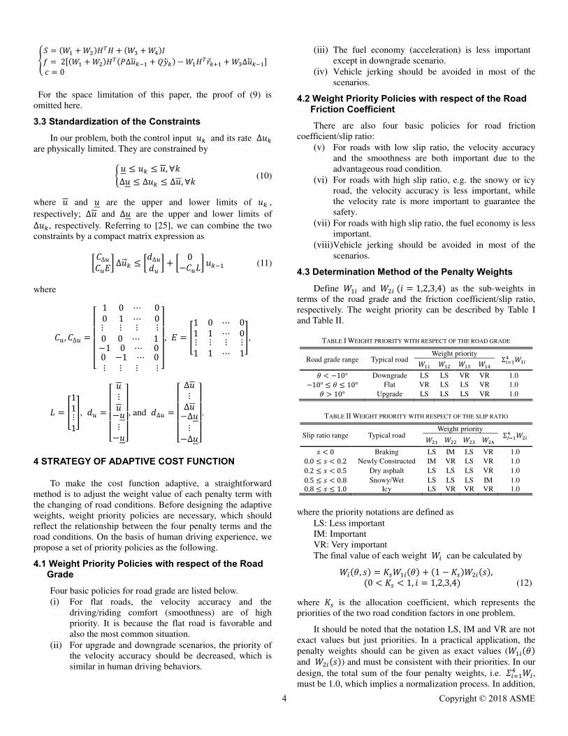
4.3 Determination Method of the Penalty Weights
Define 𝑊1𝑖 and 𝑊2𝑖 (𝑖 = 1,2,3,4) as the sub-weights in
terms of the road grade and the friction coefficient/slip ratio,
respectively. The weight priority can be described by Table I
and Table II.
TABLE I WEIGHT PRIORITY WITH RESPECT OF THE ROAD GRADE
Road grade range Typical road Weight priority Σ𝑖=14 𝑊1𝑖 𝑊11 𝑊12 𝑊13 𝑊14 𝜃 < −10° Downgrade LS LS VR VR 1.0 −10° ≤ 𝜃 ≤ 10° Flat VR LS LS VR 1.0 𝜃 > 10° Upgrade LS LS LS VR 1.0
TABLE II WEIGHT PRIORITY WITH RESPECT OF THE SLIP RATIO
Slip ratio range Typical road Weight priority Σ𝑖=14 𝑊2𝑖 𝑊21 𝑊22 𝑊23 𝑊24 𝑠 < 0 Braking LS IM LS VR 1.0 0.0 ≤ 𝑠 < 0.2 Newly Constructed IM VR LS VR 1.0 0.2 ≤ 𝑠 < 0.5 Dry asphalt LS LS LS VR 1.0 0.5 ≤ 𝑠 < 0.8 Snowy/Wet LS LS LS IM 1.0 0.8 ≤ 𝑠 ≤ 1.0 Icy LS VR VR VR 1.0
where the priority notations are defined as
LS: Less important
IM: Important
VR: Very important
The final value of each weight 𝑊𝑖 can be calculated by 𝑊𝑖(𝜃, 𝑠) = 𝐾𝑠𝑊1𝑖(𝜃) + (1 − 𝐾𝑠)𝑊2𝑖(𝑠), (0 < 𝐾𝑠 < 1, 𝑖 = 1,2,3,4) (12)
where 𝐾𝑠 is the allocation coefficient, which represents the
priorities of the two road condition factors in one problem.
It should be noted that the notation LS, IM and VR are not
exact values but just priorities. In a practical application, the
penalty weights should can be given as exact values (𝑊1𝑖(𝜃)
and 𝑊2𝑖(𝑠)) and must be consistent with their priorities. In our
design, the total sum of the four penalty weights, i.e. 𝛴𝑖=14 𝑊𝑖, must be 1.0, which implies a normalization process. In addition,
4 Copyright © 2018 ASME


The control input rates of the two strategies are shown in
Figure 2(e). It can be seen that the adaptive-weight strategy
behaves better than the fixed-weight strategy, still with a
smaller peak value.
The most important comparison of the two strategies are
presented by control costs. In the preceding optimization
process of MPC, the two curves of the cost function value
present quite different features in the amplitude. As we can
observe clearly in Figure 2(f), the total control cost of the
adaptive-weight strategy is about 49% lower than that of the
fixed-weight strategy. This percent is calculated by
𝐷𝐽 = ∑ {𝐽Fixed−weight(𝑘)−𝐽Adaptive−weight(𝑘)}𝑁𝑘=1 ∑ 𝐽Fixed−weight(𝑘)𝑁𝑘=1 × 100% (13)
where 𝑁 represents the total number of the time instants; 𝑘
represents the current time instant.
Therefore, the overall performance of the adaptive-weight
strategy is better than that of the fixed-weight strategy because,
for the same control problem the former has a better tracking
performance and at the same time a much lower control cost
than the latter.
7 CONCLUSIONS
In this paper, a road condition adaptive strategy of MPC
control has been devised based on a mechanism of adaptive
cost function. The proposed approach has been applied to the
longitudinal control problem of autonomous vehicles. The MPC
controller is solved after being converted to a QP problem. To
verify the effectiveness of the proposed approach, simulation
has been carried out on a simulated road with time-varying road
grades and friction coefficients. The results show that the
proposed approach is effective in handling different road
conditions. Using the new strategy, lower control cost can be
achieved compared with the strategy of fixed cost function.
This paper presents the application of the road condition
adaptive MPC method on the longitudinal control of
autonomous vehicles. As for future work, we will study to
apply the proposed approach to more other control problems in
autonomous vehicles such as platooning control and lateral
control, to further leverage the research outcomes.
ACKNOWLEDGEMENT
This work was supported by the National Science
Foundation Grant CRII-1755771.
REFERENCES
[1] Bansal, P., and Kockelman, K. M. “Forecasting Americans’ long-term
adoption of connected and autonomous vehicle technologies.”
Transportation Research Part A: Policy and Practice 95, 2017: 49-63.
[2] Rawlings, J. B., and Mayne, D. Q. “Model predictive control: theory and
design.” Nob Hill Pub., 2012.
[3] Waluś, K. J., and Olszewski, Z. “Analysis of tire-road contact under
winter conditions.” Proceedings of the World Congress on Engineering.
(3), 2011.
[4] Borrelli, F., Falcone, P., Keviczky, T., Asgari, J., and Hrovat, D.
“MPC-based approach to active steering for autonomous vehicle systems.”
International Journal of Vehicle Autonomous Systems, 2005, 3(2-4):
265-291.
[5] Falcone, P., Borrelli, F., Asgari, J., Tseng, H. E., and Hrovat, D.
“Predictive active steering control for autonomous vehicle systems.”
IEEE Transactions on Control Systems Technology, 2007, 15(3):566-580.
[6] Falcone, P., Borrelli, F., Tseng, H. E., Asgari, J., and Hrovat, D. “Linear
time-varying model predictive control and its application to active
steering systems: stability analysis and experimental validation.”
International Journal of Robust and Nonlinear Control, 2008, 18(8),
862-875.
[7] Turri, V., Carvalho, A., Tseng, H. E., Johansson, K. H., and Borrelli, F.
“Linear model predictive control for lane keeping and obstacle avoidance
on low curvature roads”, Intelligent Transportation Systems-(ITSC), 2013
16th International IEEE Conference, 2013: 378-383.
[8] Carvalho, A., Gao, Y., Gray, A., Tseng, H. E., and Borrelli, F. “Predictive control of an autonomous ground vehicle using an iterative linearization
approach.” Intelligent Transportation Systems-(ITSC), 2013 16th
International IEEE Conference, 2013: 2335-2340.
[9] Kamal, M. A. S., Mukai, M., Murata, J., and Kawabe, T. “Ecological driver assistance system using model based anticipation of
vehicle-road-traffic information.” IET Journal of Intelligent
Transportation Systems, 2010, 4(4): 244-251.
[10] Yi, B., Gottschling, S., Ferdinand, J., Simm, N., Bonarens, F., and Stiller,
C. “Real time integrated vehicle dynamics control and trajectory planning
with MPC for critical maneuvers”. Intelligent Vehicles Symposium (IV),
2016 IEEE 584-589.
[11] Jalalmaab, M., Pirani, M., Fidan, B., and Jeon, S. “Cooperative road
condition estimation for an adaptive model predictive collision avoidance
control strategy.” Intelligent Vehicles Symposium (IV), 2016 IEEE:
1072-1077.
[12] Beal, C. E., and Gerdes, J. C. “Model predictive control for vehicle
stabilization at the limits of handling.” IEEE Transactions on Control
Systems Technology, 2013, 21(4): 1258-1269.
[13] Chen, Y., and Wang J. “Adaptive vehicle speed control with input
injections for longitudinal motion independent road frictional condition
estimation.” IEEE Trans. on Vehicular Technology, 2011, 60(3): 839-848.
[14] Kidambi, N., Harne, R. L., Fujii, Y., Pietron, G. M., and Wang, K.
“Methods in vehicle mass and road grade estimation.” SAE International
Journal of Passenger Cars-Mechanical Systems, 2014, 7: 981-991.
[15] Han, K., Hwang, Y., Lee, E., and Choi, S. “Robust estimation of
maximum tire-road friction coefficient considering road surface
irregularity.” International Journal of Automotive Technology, 2016,17(3):
415-425.
[16] Mahyuddin, M. N., Na, J., Herrmann, G., Ren, X., and Barber, P.
“Adaptive observer-based parameter estimation with application to road
gradient and vehicle mass estimation.” IEEE Transactions on Industrial
Electronics, 2014, 61(6): 2851-2863.
[17] Rajamani, R., Phanomchoeng, G., Piyabongkarn, D., and Lew, J. Y.
“Algorithms for real-time estimation of individual wheel tire-road friction
coefficients.” IEEE/ASME Transactions on Mechatronics, 2012, 17(6): 1183-1195.
[18] Liu, Y. H., Li, T., Yang, Y. Y., Ji, X. W., and Wu, J. “Estimation of tire-road friction coefficient based on combined APF-IEKF and iteration
algorithm.” Mechanical Systems and Signal Processing, 2017, 88: 25-35.
[19] Sahlholm, P., and Johansson, K. H. “Road grade estimation for
look-ahead vehicle control using multiple measurement runs.” Control
Engineering Practice, 2010, 18(11): 1328-1341.
[20] Son, Y. S., Kim, W., Lee, S. H., and Chung, C. C. “Robust multirate
control scheme with predictive virtual lanes for lane-keeping system of
autonomous highway driving.” IEEE Transactions on Vehicular
Technology, 2015, 64(8): 3378-3391.
[21] Li, S., Li, K., Rajamani, R., and Wang, J. “Model predictive
multi-objective vehicular adaptive cruise control. IEEE Transactions on
Control Systems Technology.” 2011, 19(3): 556-566.
[22] Biron, Z. A., and Pisu, P. “Distributed fault detection and estimation for
cooperative adaptive cruise control system in a platoon.” In PHM
Conference, 2015.
[23] Shakouri, P., Ordys, A., and Askari, M. R. “Adaptive cruise control with
stop&go function using the state-dependent nonlinear model predictive
control approach.” ISA Transactions, 2012, 51(5): 622-631.
[24] Rossiter, J. A., and Kouvaritakis, B. “Constrained stable generalised
predictive control.” In IEE Proceedings D-control Theory and
Applications 1993, 140 (4): 243-254.
[25] Rossiter J. A. Model-based predictive control: a practical approach. CRC
press, 2003.
6 Copyright © 2018 ASME


![Copy ShaneCoCatalog2 [Read-Only]](https://img.pdfslide.us/doc/110x75/55c4af1abb61eb7e118b45fc/copy-shanecocatalog2-read-only.jpg)
![mc ch07 - Copy [Read-Only]](https://img.pdfslide.us/doc/110x75/616d919bfa7c607c344313ad/mc-ch07-copy-read-only.jpg)