Attempting Consistent Simulations of Stn. ALOHA with a ... · sured as PP. In this study we test the hypothesis that, by includ-ing overflow production of DOC in a multi-element eco-system

1

Journal of Oceanography, Vol. 61, pp. 1 to 23, 2005

Keywords:⋅⋅⋅⋅⋅ Model,⋅⋅⋅⋅⋅ ecosystem,⋅⋅⋅⋅⋅ biogeochemical,⋅⋅⋅⋅⋅ stoichiometry.

* Corresponding author. E-mail: [email protected]

Copyright © The Oceanographic Society of Japan.

Attempting Consistent Simulations of Stn. ALOHA witha Multi-Element Ecosystem Model

S. LAN SMITH1*, YASUHIRO YAMANAKA2 and MICHIO J. KISHI3

1Global Warming Group, Frontier Research System for Global Change, Yokohama 236-0001, Japan2Graduate School of Environmental Earth Science, Hokkaido University, Sapporo 060-0810, Japan3Faculty of Fisheries, Hokkaido University, Hakodate 041-8611, Japan

(Received 12 August 2003; in revised form 13 January 2004; accepted 14 April 2004)

We used a one dimensional, multi-element model to simulate the primary production(PP), recycling and export of organic matter at Stn. ALOHA, near Hawaii. We com-pared versions of the model with and without the cycling of dissolved organic matter(DOM) via the Microbial Food Web (MFW). We incorporated recently publishedmeasurements of high C:N ratios for uptake by diazotrophs. For other phytoplanktonwe included a formulation for overflow production of dissolved organic carbon (DOC),which occurs under nutrient-limited, light-replete conditions. We were able to matchthe observed mean DOC profile near the surface with both models, by tuning only thefraction of overflow DOC that is labile. The simulated bulk C:N remineralizationratio from the MFW model agreed well with a data-based estimate for the NorthPacific subtropical gyre, but that from the Base model was too low. This is becausethe MFW model includes bacteria, with their low-C:N biomass. Simulated mean PPwas lower than observed by 10% (Base) and 27% (MFW). This is consistent with theexpectation that the 14C-method measures something greater than net production.DOC accounted for approximately half of simulated PP, most of this being overflowDOC. We find that overflow production and the MFW are key processes for reconcil-ing the various data and PP measurements at this oligotrophic site. The impact ofbacteria on the C:N remineralization ratio is an important link between ecosystemstructure and the cycling of carbon.

Spitz et al., 2001) or nitrogen- and phosphorus-based(Fennel et al., 2002) models to this location or to theBermuda Atlantic Time Series (BATS) site. Recent mod-els that included N2 fixation have yielded improvedsimulations of the nitrogen cycle at BATS (Hood et al.,2001) and at Stn. ALOHA (Fennel et al., 2002). Spitz etal. (2001) assimilated data from BATS into models ofvarying complexity and found that bacteria were key tocontrolling the size of the DOM pool and regeneratedproduction. They concluded that a better conversion fromN to C was necessary for simulating the carbon cycle.

The models above did not consistently simulate themeasured PP and fluxes of POM. Hood et al. (2001) couldtune their model to simulate either the observed DICdrawdowns and N2 fixation rates, or the observed fluxesof particulate organic nitrogen (PON), but not both. Evenwith data assimilation, the Spitz et al. (2001) model in-cluding bacteria matched the POC fluxes well but simu-lated PP that was significantly lower than observed.Fennel et al. (2002) could well simulate the distribution

1. IntroductionTo simulate such changes in biogeochemical cycles

as may result from changes in global climate, we seekmore mechanistic models of biogeochemical processes.With this study we aimed to examine how well we couldconsistently simulate the various data for nutrients, DOM,POM fluxes, and primary production (PP) available atStn. ALOHA. We focused particularly on consistentlysimulating carbon and nutrient cycles. We chose this sitebecause of the large quantity of data available and theextent of oligotrophic areas similar to this site in theocean.

1.1 Recent time-series simulationsSeveral studies have applied nitrogen-based (Doney

et al., 1996; Hurtt and Armstrong, 1996; Hood et al., 2001;

2 S. L. Smith et al.

of Trichodesmium and their N2 fixation rates, while match-ing the mean observed PON flux. However, for the fouryears simulated their net rate of organic matter produc-tion by phytoplankton and diazotrophs (uptake-respira-tion, from figure 13 in Fennel et al. (2002)) is 155 mmolesN m–2 yr–1. To support the observed C-based PP of ap-proximately 480 mg C m–2 d–1 (14,600 mmoles C m–2

yr–1) would require an average C:N ratio of 94 for pro-duction. DOC production may be the key to reconcilingthe simulations of the nitrogen cycle with the PP meas-urements.

1.2 Simulating DOMGlobal modeling studies have found that including

Dissolved Organic Matter (DOM) reduced the problemof nutrient trapping (Najjar et al., 1992; Yamanaka andTajika, 1997). In their global biogeochemical model,Yamanaka and Tajika (1997) found that dividing the DOM(as Dissolved Organic Phosphorus, DOP, in their model)into two classes (semi-labile and refractory) improvedtheir simulations of the global distributions of phosphateand 14C. They simulated well the global patterns of thosetracers using a first order decay rate coefficient of 0.5per year for semi-labile DOP and 1/65 per year for re-fractory DOP in the euphotic layer (assuming that the re-fractory material was not degraded below the euphoticlayer).

Connolly et al. (1992) summarized various data andmodel formulations for biodegradation. The formulationsgenerally divide dissolved organic matter into labile andsemi-labile fractions and use Michaelis-Menten kineticsto represent the degradation rates of each class. Rates ofbacterially-mediated remineralization of DOM can be lim-ited both by temperature and by the concentration of DOM(Connolly et al., 1992; Kirchman and Rich, 1997). Dif-ferent rates of degradation have been measured for dif-ferent classes of dissolved and colloidal organic matter,and even for the same proteins when adsorbed into bio-logical membranes as opposed to freely dissolved (Nagataand Kirchman, 1997; Nagata et al., 1998). Grazing ofbacteria by microzooplankton (Rivkin et al., 1999) mightalso contribute to spatial and temporal variations inremineralization rate. Shinada et al. (2000) have recentlymeasured seasonally-varying rates of phytoplankton graz-ing by microzooplankton. They found evidence indicat-ing that bacteria may provide the primary food source formicro-zooplankton during summer in the Oyashio regionof the western North Pacific. This grazing pressure onbacterial growth would also limit the rate at which DOMis remineralized. Much evidence suggests that a mecha-nistic model of carbon and nutrient cycling in the oceanshould include some representation of bacteria.

Some models (Fasham et al., 1993; Pondaven et al.,2000) have included bacteria as a component, with the

remineralization rate of DOM depending on the concen-tration of bacteria. Still, many models do not explicitlyaccount for the dependence of DOM remineralization rateon bacteria (e.g., Oschlies et al., 2000). Popova andAnderson (2002) compared simulations using a globalbox-model with and without DOM (both without bacte-ria). They found small but significant differences in PPand alkalinity, but concluded that for some purposes anexplicit representation is probably unnecessary. Pondavenet al. (2000) compared an ecosystem model formulationwith an explicit representation of bacteria and DON cy-cling to one without it. They found that the basic modelbehavior, including the simulated PP, was not significantlydifferent for the two formulations. They did find that in-cluding the bacterial formulation allowed them to repro-duce an observed subsurface maximum in ammonium thatwas not reproduced with the non-bacterial model. Oschlieset al. (2000) used an ecosystem model embedded in aneddy-permitting 3-D physical model to simulate the NorthAtlantic. Their simulated PP was too low in oligotrophicregions, and they suggested including more efficient re-cycling as a possible remedy for this.

Given the high concentrations of DOM at Stn.ALOHA and its importance in nutrient cycling, we de-cided to compare a version of the ecosystem model witha simple formulation for DOM to one with a more elabo-rate formulation for cycling of DOM via bacteria basedon the microbial food web (MFW) model of Andersonand Williams (1998) (hereafter, AW98).

1.3 Overflow production of DOCBecause of their peculiar biochemistry, diazotrophs

(N2 fixing organisms) may contribute greatly to the Ccycle as well as the N cycle in oligotrophic areas. Orcuttet al . (2001) measured C:N uptake ratios forTrichodesmium at the BATS site and found a mean ratioof 128, with some values being nearly four times thatlevel. The mean value is roughly 20 times the Redfieldratio of 6.6. This is an interesting result that deserves moreattention. They suggested that this high uptake ratio mayhelp explain the observed drawdown of DIC despite lowconcentrations of nutrients at BATS. If this is the casefor Trichodesmium in general, it could explain some ofthe high measured 14C PP at Stn. ALOHA, where theseorganisms are plentiful. Higher-than-Redfield ratios forthe uptake of C:N have been observed for otherphytoplankton, too. Pennock (1987) measured uptake ra-tios for C:N of 13 (averaged over daylight) and 8.4 (aver-aged over the diel cycle) for phytoplankton in the Dela-ware estuary. The most likely explanation for these highuptake ratios is overflow production of DOC (but notDON or DOP), which occurs when nutrients are limitingbut light is plentiful. There is a physiological basis foroverflow production of DOC via photorespiration, as dis-

Attempting Consistent Simulations 3

cussed by Geider and MacIntyre (2002), which may serveto reduce oxidative stress at high irradiances (Kozaki andTakeba, 1996).

Overflow DOC should contribute significantly to PPmeasured with the 14C-method. Karl et al. (1998), in astudy of how much DOC was measured on the filters usedin such experiments, found that on average 54% of 14C-DOC passing through less adsobent filters also passedthrough the filters used for PP measurements (on onecruise in 1997). Thus, a minimum of 46% of the 14C-DOCwas trapped by the filters, meaning that it would be mea-sured as PP.

In this study we test the hypothesis that, by includ-ing overflow production of DOC in a multi-element eco-system model, we can consistently simulate the cycles ofnutrients and organic matter, together with the PP meas-urements from Stn. ALOHA.

2. Biogeochemcial ModelOur earlier simulations (unpublished) with a nitro-

gen-based ecosystem model gave reasonable simulationsof mean PON fluxes, but did not agree well with the mea-sured PP. To improve simulations of the cycling of DON,we embedded the formulation from AW98 for the MFW.This worked, but did not improve the simulations of PP.Embedding the Fennel et al. (2002) model for N2 fixa-tion at Stn. ALOHA improved the simulations somewhat,but required the addition of a phosphorus cycle becauseP limits the growth of diazotrophs in their model. This,together with the high DOC:DON and DON:DOP ratios

observed in the shallow waters at this site, motivated ourchoice to include C, N and P cycles explicitly in the model.With this we aimed for more consistent simulations ofthe various data and more constraints on the model.

Here we use a multi-element model including C, N,P and Si cycles. We developed this model based on theN-based NEMURO formulation (Eslinger et al., 2000;Fujii et al., 2002a (hereafter, FNYK); Yamanaka et al.,2004). NEMURO consists of 11 compartments (two typesof phytoplankton, three types of zooplankton, nitrate,ammonium, DON, PON, dissolved silicate and biogenicsilica). Like most such ecosystem models (e.g., Fashamet al., 1993; Kawamiya et al., 1997; Denman and Pena,1999; Kishi et al., 2001), it includes compartments rep-resenting phytoplankton, zooplankton, nutrients and or-ganic matter. We also divided POM into suspended(SPOM) and sinking (POM) fractions. We included over-flow production of DOC, which impacts both simulatedDOC and PP.

With the additions above we have our Base Model.We have also developed a version that includes the cy-cling of DOM via the MFW.

2.1 Base modelFigure 1 is a diagram of the components and flows

in the Base model, and Appendix A lists the full set ofequations.

We assumed fixed stoichiometries for all living or-ganisms (Table 1). Only the nitrogen concentration issimulated for each compartment representing living or-

N:P:Si Ecosystem Model

Biogeochemical Processes

+ Physical Processes (1-D Mellor-Yamada model)

Predation

Pre

datio

n

Preda

tion

Si(OH)4

Photosysthesis

Respiration

Respiration

Extrac

ellula

r

Excre

tion

Extracellular Excretion

Extracellular

Excretion

Nitrification

Decomposition

Remineralization

Respiration

Mor

talit

y

Mort.

Mortality

Mor

talit

y

Mor

talit

y

Grazing

Grazing

Grazin

g

Egestion

Ege

stio

n Ege

stio

n

Sin

king

Sin

king

LargeZooplankton

PredatoryZooplankton

SmallZooplankton

LargePhytoplankton

Decomposition

Excre

tion

ZL

Egestion

Si flowN & P flow

PS ZS

POMDOM

RespirationExcretion

NO3

Photo-systhesisNH4

DIP

OpalPhotosysthesis

PL

Grazing

Mor

talit

y

Ege

stio

n

Extracellular

ExcretionMortalityR

emin

eral

-

izat

ion

Pho

tosy

sthe

sis

ZP

SmallPhytoplankton

DiazoDiazotrophs

Fig. 1. Diagram of the compartments and flows in the ecosystem model.


ganisms. Separate compartments are simulated for eachelement in nonliving organic matter (e.g., DOC, DON andDOP). Rates of degradation of the elemental fractions aredirectly proportional to their stoichiometries (which canvary). All rates depend exponentially on temperature,except for the diazotrophs’ growth rate, which followsFennel et al. (2002).

Organic matter is produced with varying stoichiom-etry because of the distinct stoichiometries ofzooplankton, diazotrophs and other phytoplankton. As thediet of a given zooplankton changes, the stoichiometryof its uptake will change. The fixed stoichiometry of itsbiomass (in the model) requires that the stoichiometry ofits output must vary. We assume that the output stoichi-ometries of egestion, excretion and respiration are thesame. The output C:N ratio for zooplankton Z (=ZS, ZLor ZP, for small, large and predatory zooplankton, respec-tively; see Fig. 1) is calculated as:

RCN

RCN G P Z RCN G P Z

Ege R

Zout

P P Z Z Z P Z

Z Z

Z Z Z=⋅ ( )[ ] − ⋅ ⋅ ( )

+( ) ( )Σ Σ, ,β

1

G(PZ, Z) is the rate of grazing of prey PZ by Z. The sumover PZ counts all prey for each Z. RCNPZ

is the C:Nratios of prey PZ. βZ is the gross growth efficiency of Z.EgeZ and RZ are the rates of egestion of PON andremineralization of NH4, respectively. The output N:Pratios are calculated similarly. Because the stoichiometries

of all organisms are fixed, these mass balances apply in-stantaneously.

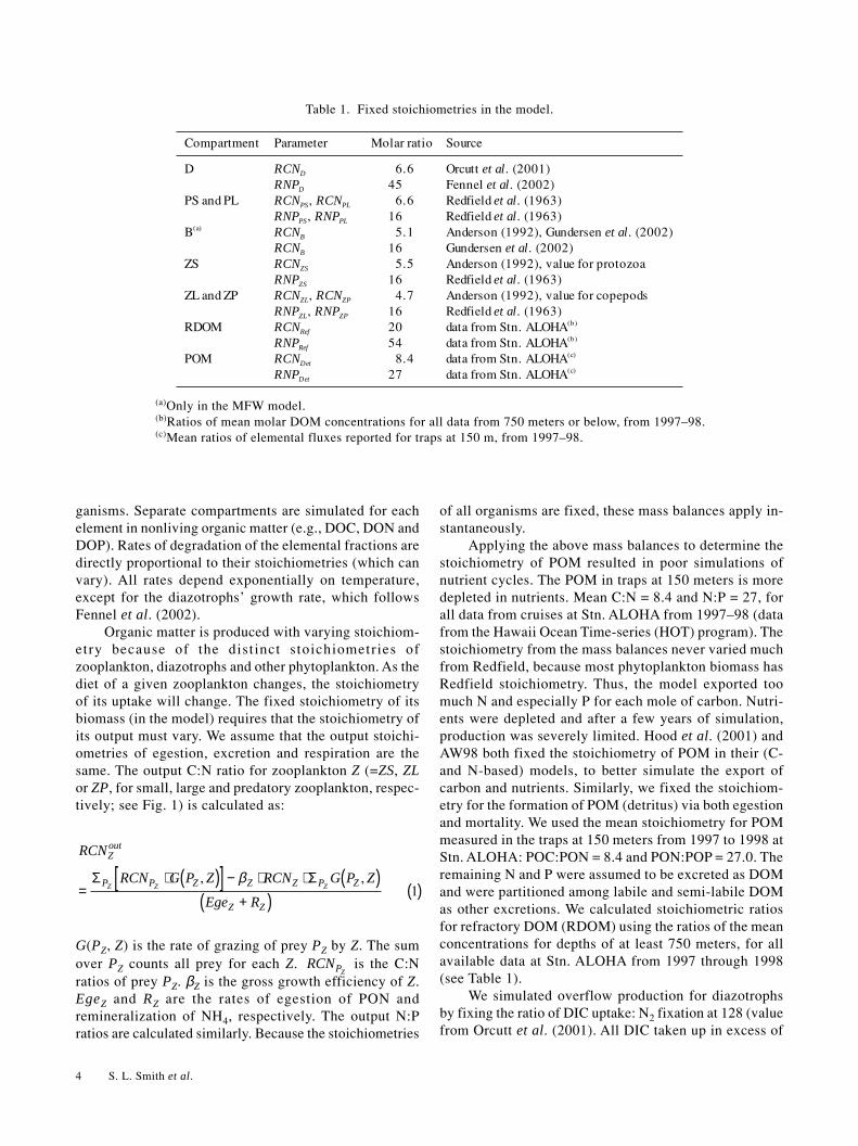
Applying the above mass balances to determine thestoichiometry of POM resulted in poor simulations ofnutrient cycles. The POM in traps at 150 meters is moredepleted in nutrients. Mean C:N = 8.4 and N:P = 27, forall data from cruises at Stn. ALOHA from 1997–98 (datafrom the Hawaii Ocean Time-series (HOT) program). Thestoichiometry from the mass balances never varied muchfrom Redfield, because most phytoplankton biomass hasRedfield stoichiometry. Thus, the model exported toomuch N and especially P for each mole of carbon. Nutri-ents were depleted and after a few years of simulation,production was severely limited. Hood et al. (2001) andAW98 both fixed the stoichiometry of POM in their (C-and N-based) models, to better simulate the export ofcarbon and nutrients. Similarly, we fixed the stoichiom-etry for the formation of POM (detritus) via both egestionand mortality. We used the mean stoichiometry for POMmeasured in the traps at 150 meters from 1997 to 1998 atStn. ALOHA: POC:PON = 8.4 and PON:POP = 27.0. Theremaining N and P were assumed to be excreted as DOMand were partitioned among labile and semi-labile DOMas other excretions. We calculated stoichiometric ratiosfor refractory DOM (RDOM) using the ratios of the meanconcentrations for depths of at least 750 meters, for allavailable data at Stn. ALOHA from 1997 through 1998(see Table 1).

We simulated overflow production for diazotrophsby fixing the ratio of DIC uptake: N2 fixation at 128 (valuefrom Orcutt et al. (2001). All DIC taken up in excess of

Compartment Parameter Molar ratio Source

D RCND 6.6 Orcutt et al. (2001)RNPD 45 Fennel et al. (2002)

PS and PL RCNPS, RCNPL 6.6 Redfield et al. (1963)RNPPS, RNPPL 16 Redfield et al. (1963)

B(a) RCNB 5.1 Anderson (1992), Gundersen et al. (2002)RCNB 16 Gundersen et al. (2002)

ZS RCNZS 5.5 Anderson (1992), value for protozoaRNPZS 16 Redfield et al. (1963)

ZL and ZP RCNZL, RCNZP 4.7 Anderson (1992), value for copepodsRNPZL, RNPZP 16 Redfield et al. (1963)

RDOM RCNRef 20 data from Stn. ALOHA(b)

RNPRef 54 data from Stn. ALOHA(b)

POM RCNDet 8.4 data from Stn. ALOHA(c)

RNPDet 27 data from Stn. ALOHA(c)

Table 1. Fixed stoichiometries in the model.

(a)Only in the MFW model.(b)Ratios of mean molar DOM concentrations for all data from 750 meters or below, from 1997–98.(c)Mean ratios of elemental fluxes reported for traps at 150 m, from 1997–98.


their biomass stoichiometry (C:N = 6.6, as reported byOrcutt et al. (2001)) was assumed to be overflow DOCproduction. For other phytoplankton, we used the formu-lation of AW98, the key assumption of which is that whennutrient-limitation exceeds light-limitation, plankton willproduce organic compounds containing carbon only. Theformulation is:

E f T L I P GPPPovf

ofv P phy P P= ⋅ ⋅ ( ) ⋅ ( ) ⋅( ) − ( )µ Θ . 2

As in AW98, fofv is an adjustable parameter, which multi-plies the difference between the light-limited(µP·Θphy(T)·LP(I)·P) and light-and-nutrient-limited(GPPP) growth rates. Increasing fofv increases both theconcentration of DOC and PP. The turnover time of over-flow DOC is controlled by parameter δovf2L, which is thefraction of overflow DOC that is labile (the rest beingsemi-labile, see Appendix A). In the Base model, the la-bile fraction is assumed to be remineralized instantane-ously. In the MFW model, the turnover time for labileDOC (LDOC) is on the order of a day. Increasing δovf2Lreduces the impact of overflow production on the meanDOC profile (and on the bulk DOC:DON ratio). δovf2L doesnot change simulated PP, however, for which all DOCcounts equally.

2.2 MFW modelAW98’s coupled one-dimensional, physical-bio-

chemical model simulates the concentrations of twoclasses each of DOC and DON and one class of bacteria,for a total of five compartments. Remineralization of la-bile LDOM and hydrolysis of semi-labile SDOM (to formLDOC) depend on the concentration of bacteria, withMonod-type rate expressions for the rates of degradation.We have embedded this model into our ecosystem model

to construct our MFW model.Pursuant to our ultimate goal of simulating the ef-

fects of climate change on the oceanic carbon cycle, andfor consistency with the NEMURO formulation, we modi-fied all rate expressions to include exponential tempera-ture dependence, as in Eppley (1972). For most rates, aQ10 of 2.0 was applied. As in AW98, we assume that re-fractory DOM is constant, which is reasonable forsimulations shorter than a few hundred years (Andersonand Williams, 1999).

We added compartments for N and P in each class ofDOM (e.g., for labile (LDOM), we added LDON andLDOP). Degradation rates are carbon-based, as in AW98.The N and P in each class of DOM are degraded withrates proportional to its stoichiometry, as described abovefor remineralization in the Base model. Analogous to themass balances used for zooplankton, instantaneous massbalances determine the stoichiometries for LDOM pro-duction (via hydrolysis of SDOM) and remineralizationof LDOM. Appendix B presents the equations and de-scribes the model in detail.

2.3 Parameter valuesValues for biological parameters are listed in Table

2 for diazotrophs, in Table 3 for other phytoplankton, inTable 4 for zooplankton. Table 5 lists other general pa-rameters. Values were based on those in FNYK, whichsimulated the Stn. KNOT site in the northwestern Pacific.For small phytoplankton, half-saturation coefficients fornitrate and ammonium were lowered to get the simulatednutrient profiles to agree with the data. We maintainedthe 10 ratio of the half-saturation coefficients for nitrateand ammonium, as in FNYK. This maintained the samerelative preference for ammonium over nitrate. For up-take of DIP by phytoplankton (other than diazotrophs),we used half-saturation values from the simulations of

Table 2. Parameters for diazotrophs(a).

(a)From Fennel et al. (2002) unless otherwise noted.(b)From Hood et al. (2001).

Parameter Value Units Description

µD 0.3 day–1 maximum growth rate at 0°C

αD 0.01 day–1 (W m–2)–1 initial production-irradiance slope

Tc,D 24.5 °C critical temperature for growthτc,D 0.62 dynes cm–2 critical wind stress for growth

KDIP,D 0.0004 µmol P liter–1 half-saturation constant for DIP uptake

γD 0.3(b) ratio of excretion to gross production

Dmin 0.01 µmol N liter–1 minimum concentration (for mortality)

mD 0.0088 day–1 mortality rate at 0°CrD 0.046 day–1 (µmol N liter–1)–1 rate coefficient for respiration at 0°C


Moore et al. (2002) of the global surface ocean. Othergeneral parameters are in Table 5, and Table 6 lists pa-rameters for the MFW model.

In their comparative simulations of Station Papa andBATS, Kawamiya et al. (1997) used a settling velocity of6.5 m day–1 for BATS, compared to their values of 20–100 m day–1 for Station Papa. Hurtt and Armstrong (1996)used a maximum settling velocity of 11 m day–1 in theirsimulations of the BATS site, and Hood et al. (2001) intheir simulation of BATS, used sinking velocities of 4and 12 m day–1. Thus, 40 m day–1 seems too large to rep-resent all POM at Stn. ALOHA. Fennel et al. (2002) used2.5 m day–1, with a slow decay rate for POM. They thusobtained a remineralization length scale of 250 m, con-sistent with the solubilization length scales for POM cal-culated by Christian et al. (1997).

For sinking POM, we applied FNYK’s settling ve-locity of 40 m day–1. We used rate expressions from themodel of POM degradation developed by Fujii et al.(2002b). They measured rates of degradation of POM overa range of initial organic matter concentrations from 2.4to 71 mg C liter–1, and were able to simulate their obser-vations (at 20°C) quite well using distinct first-order rates

for what they termed labile and semi-refractory POM,together with a parameter for the fraction of semi-refrac-tory POM. Fitting their data, they found that 13% of thePOC was semi-refractory at the start of their experiments.We treated all POM as equivalent to the labile fraction intheir model (87% of the total POC at the start of theirexperiments). We used their rate coefficient of 0.13day–1 at 20°C with a Q10 of 2.0 (equivalent to 0.0325day–1 at 0°C) and assumed that POM decays into DOM.Further studies (personal communication, Yoshimi Suzukiof Shizuoka University) over a range of temperatures veri-fied that the degradation is well described by a Q10 of2.0. The remineralization length scale for our sinkingPOM is thus (40 m day–1)/0.13 day–1 = 308 m (assumingan average temperature of 20°C), only slightly greaterthan Fennel et al. (2002)’s 250 m.

We based all parameters asociated with bacteria andDOM on those of AW98 (Table 6), with modificationsfor the effect of temperature and conversions from C-based to N-based units as necessary. We assumed thatAW98’s rates, for their simulations of the English Chan-nel, applied at 10°C, which was their assumption in cal-culating their rate of bacterial mortality. From this we


Small phytoplankton, PSµPS 0.3 day–1 maximum growth rate at 0°C

γPS 0.135 ratio of excretion to gross productionK PSNO3, 0.3(b) µmol N liter–1 half-saturation constant for NO3 uptakeK PSNH4 , 0.03(b) µmol N liter–1 half-saturation constant for NH4 uptake

KDIP,PS 0.00025(c) µmol P liter–1 half-saturation constant for DIP uptake

mPS 0.0585 day–1 (µmol N liter–1)–1 mortality rate coefficient at 0°C

Large phytoplankton, PLµPL 0.6 day–1 maximum growth rate at 0°C

γPL 0.135 ratio of excretion to gross productionK PLNO3, 3.0 µmol N liter–1 half-saturation constant for NO3 uptakeK PLNH4 , 0.3 µmol N liter–1 half-saturation constant for NH4 uptake

KDIP,PL 0.00125(c) µmol P liter–1 half-saturation constant for DIP uptake

KSi,PL 6.0 µmol Si liter–1 half-saturation constant for DSi uptake

mPL 0.0293 day–1 (µmol N liter–1)–1 mortality rate coefficient at 0°C

Common for PS and PLIopt,phy 105 W m–2 optimum irradianceIphy 0.03 day–1 respiration rate at 0°CΨphy 1.5 (µmol N liter–1)–1 parameter for NH4 inhibition of NO3 uptake

Table 3. Parameters for phytoplankton(a).

(a)From Fujii et al. (2002a) (FNYK), unless otherwise noted.(b)Adjusted in this study, see text.(c)From Moore et al. (2002).


calculated maximum rates at 0° C (Table 3). The rates ofremineralization of LDOC and of hydrolysis of SDOCwere also converted from rates per mole of C-based bac-terial biomass to rates per N-based bacterial biomass.

We set the fraction of grazing lost to DOM via sloppyfeeding to be consistent with the recent measurements ofSteinberg et al. (2002). They measured excretion of DONand ammonium in incubations with three types ofzooplankton from the BATS site. The average percent oftotal dissolved nitrogen (TDN) released as DON was 22%for copepods (P. xiphias) and 26% for euphausiids (N.flexipes). The ZL compartment in our model representscopepods (and zooplankton of similar trophic level) andZP represents euphausiids (and zooplankton of similartrophic level). We chose an intermediate value of 24%,which is essentially the same as the value used by Fashamet al. (1990) (hereafter, FDM). We defined parameter δsfas the fraction of unassimilated grazing that becomesDOM. Total TDN excretion as a fraction of total grazingis then sloppy feeding, δsf·(1 – αZ), plus remineralization,(αZ – βZ). To have 24% of TDN excretion as DON thusrequires δsf·(1 – αZ)/[δsf·(1 – α) + (αZ – βZ)] = 0.24, orδsf = [0.24·(αZ – βZ)]/[(1 – 0.24)·(1 – αZ)]. In the param-eter set used by FNYK, assimilation efficiencies, αZ =0.7, and growth efficiencies, βZ, = 0.3, for all zooplankton,which gives δsf = 0.42. We are not aware of any measure-

ments of excretion for microzooplankton and hetero-trophic nanoflagellates (ZS in the model), and we assumedthe same δsf as for the others.

Mortality of phytoplankton and zooplankton must bepartitioned amoung POM, DOM and remineralization.Phytoplankton die from viral infections, with lysis of thecells releasing DOM. Based on AW98’s assumption that34% of phytoplankton mortality becomes DOM, we de-fine ΩP = 0.66 and assume that the remainder becomesDOM. The value for zooplankton is smaller because themortality terms represent a chain of grazing by organ-isms not included in the model. AW98 calculated theirvalue for the fraction of zooplankton mortality becomingPOM, Ω = 0.125, so that their model would maintain thesame production ratio of ammonium to POM (7:1) as inFDM. FDM calculated their value, Ω = 0.33, assumingthat zooplankton mortality represents an infinite, instan-taneous chain of grazing. The key difference between thetwo was that AW98 accounted for production of DOMvia sloppy feeding. Assuming such a chain of grazing viaour formulation, the fraction of zooplankton mortalitybecoming DOM is δsf·(1 – α)/(1 – βZ) = 0.18 with theparameters used. The fraction remineralized is (αZ – βZ)/(1 – βZ) = 0.57, and that becoming POM is (1 – δsf)·(1 –α)/(1 – βZ) = 0.25. The ratio of ammonium to detritusproduced (via mortality of zooplankton) is thus 2.3.


Small zooplankton, ZSgB2ZS 1.0 day–1 maximum grazing rate of B at 0°CgPS2ZS 1.0 day–1 maximum grazing rate of PS at 0°C

Large zooplankton, ZLgPS2ZL 0.25 day–1 maximum grazing rate of PS at 0°CgPL2ZL 1.0 day–1 maximum grazing rate of PL at 0°CgZS2ZL 1.0 day–1 maximum grazing rate of ZS at 0°C

Predatory zooplankton, ZPgPL2ZP 0.5 day–1 maximum grazing rate of PL at 0°CgZS2ZP 0.5 day–1 maximum grazing rate of ZS at 0°CgZL2ZP 0.5 day–1 maximum grazing rate of ZL at 0°C

Common to all zooplanktonαZ 0.7 assimilation efficiency

βZ 0.3 growth efficiency

λ I 1.4 (µmol N liter–1)–1 Ivlev constant

mZoo 0.0585 day–1 (µmol N liter–1)–1 mortality rate at 0°C

Bmin 0.020 µmoles N minimum biomass for grazing B

Pmin 0.043 µmoles N minimum biomass for other prey, P

Table 4. Parameters for zooplankton(a).

(a)From Fujii et al. (2002a) (FNYK).


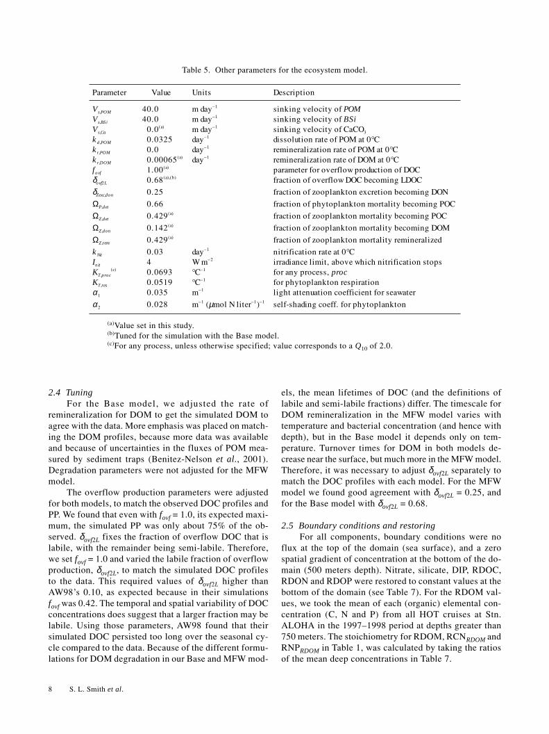
2.4 TuningFor the Base model, we adjusted the rate of

remineralization for DOM to get the simulated DOM toagree with the data. More emphasis was placed on match-ing the DOM profiles, because more data was availableand because of uncertainties in the fluxes of POM mea-sured by sediment traps (Benitez-Nelson et al., 2001).Degradation parameters were not adjusted for the MFWmodel.

The overflow production parameters were adjustedfor both models, to match the observed DOC profiles andPP. We found that even with fovf = 1.0, its expected maxi-mum, the simulated PP was only about 75% of the ob-served. δovf2L fixes the fraction of overflow DOC that islabile, with the remainder being semi-labile. Therefore,we set fovf = 1.0 and varied the labile fraction of overflowproduction, δovf2L, to match the simulated DOC profilesto the data. This required values of δovf2L higher thanAW98’s 0.10, as expected because in their simulationsfovf was 0.42. The temporal and spatial variability of DOCconcentrations does suggest that a larger fraction may belabile. Using those parameters, AW98 found that theirsimulated DOC persisted too long over the seasonal cy-cle compared to the data. Because of the different formu-lations for DOM degradation in our Base and MFW mod-

els, the mean lifetimes of DOC (and the definitions oflabile and semi-labile fractions) differ. The timescale forDOM remineralization in the MFW model varies withtemperature and bacterial concentration (and hence withdepth), but in the Base model it depends only on tem-perature. Turnover times for DOM in both models de-crease near the surface, but much more in the MFW model.Therefore, it was necessary to adjust δovf2L separately tomatch the DOC profiles with each model. For the MFWmodel we found good agreement with δovf2L = 0.25, andfor the Base model with δovf2L = 0.68.

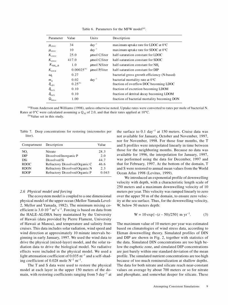
2.5 Boundary conditions and restoringFor all components, boundary conditions were no

flux at the top of the domain (sea surface), and a zerospatial gradient of concentration at the bottom of the do-main (500 meters depth). Nitrate, silicate, DIP, RDOC,RDON and RDOP were restored to constant values at thebottom of the domain (see Table 7). For the RDOM val-ues, we took the mean of each (organic) elemental con-centration (C, N and P) from all HOT cruises at Stn.ALOHA in the 1997–1998 period at depths greater than750 meters. The stoichiometry for RDOM, RCNRDOM andRNPRDOM in Table 1, was calculated by taking the ratiosof the mean deep concentrations in Table 7.

Table 5. Other parameters for the ecosystem model.

(a)Value set in this study.(b)Tuned for the simulation with the Base model.(c)For any process, unless otherwise specified; value corresponds to a Q10 of 2.0.


Vs,POM 40.0 m day–1 sinking velocity of POMVs,BSi 40.0 m day–1 sinking velocity of BSiVs,Ca 0.0(a) m day–1 sinking velocity of CaCO3

k d ,POM 0.0325 day–1 dissolution rate of POM at 0°Ck r,POM 0.0 day–1 remineralization rate of POM at 0°Ck r,DOM 0.00065(a) day–1 remineralization rate of DOM at 0°Cfovf 1.00(a) parameter for overflow production of DOCδovf2L 0.68(a),(b) fraction of overflow DOC becoming LDOC

δZexc,don 0.25 fraction of zooplankton excretion becoming DON

ΩP,det 0.66 fraction of phytoplankton mortality becoming POC

ΩZ,det 0.429(a) fraction of zooplankton mortality becoming POC

ΩZ,don 0.142(a) fraction of zooplankton mortality becoming DOM

ΩZ,rem 0.429(a) fraction of zooplankton mortality remineralized

k Nit 0.03 day–1 nitrification rate at 0°CInit 4 W m–2 irradiance limit, above which nitrification stopsKT,proc

(c) 0.0693 °C–1 for any process, procKT,res 0.0519 °C–1 for phytoplankton respirationα 1 0.035 m–1 light attenuation coefficient for seawater

α 2 0.028 m–1 (µmol N liter–1)–1 self-shading coeff. for phytoplankton


2.6 Physical model and forcingThe ecosystem model is coupled to a one dimensional

physical model of the upper ocean (Mellor-Yamada Level-2, Mellor and Yamada, 1982). The minimum mixing co-efficient is 3.0·10–5 m2 s–1. Forcing is based on data fromthe HALE-ALOHA buoy maintained by the Universityof Hawaii (data provided by Pierre Flament, Universityof Hawaii at Manoa), and temperature and salinity fromcruises. This data includes solar radiation, wind speed andwind direction at approximately 10 minute intervals be-ginning in early January, 1997. We used the wind data todrive the physical (mixed-layer) model, and the solar ra-diation data to drive the biological model. No radiativeeffects were included in the physical model. We used alight attenuation coefficient of 0.035 m–1 and a self-shad-ing coefficient of 0.028 mole N–1 m–1.

The T and S data were used to restore the physicalmodel at each layer in the upper 150 meters of the do-main, with restoring coefficients ranging from 5 day–1 at

the surface to 0.1 day–1 at 150 meters. Cruise data wasnot available for January, October and November, 1997,nor for November, 1998. For those four months, the Tand S profiles were interpolated linearly in time betweenthose for the neighboring months. Because no data wasavailable for 1996, the interpolation for January, 1997,was performed using the data for December, 1997 andthat for February, 1997. At the bottom of the domain, Tand S were restored to annual mean values from the WorldOcean Atlas 1998 (Levitus, 1999).

We introduced an exponential profile of downwellingvelocity with depth, with a characteristic length scale of250 meters and a maximum downwelling velocity of 10meters per year. This velocity was ramped linearly to zeroover the upper 50 m of the domain, to ensure zero veloc-ity at the sea surface. Thus, for the downwelling velocity,W, below 50 meters depth:

W = 10·exp–(z – 50)/250 m yr–1. (3)

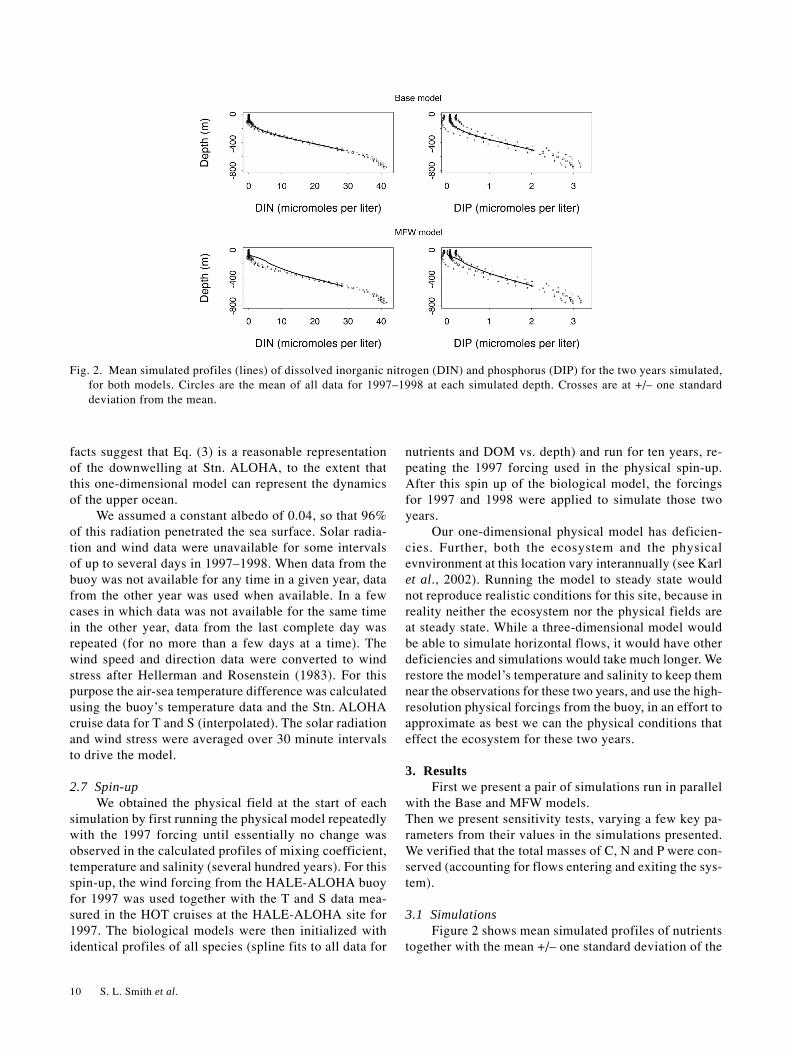
The maximum value of 10 meters per year was estimatedbased on climatologies of wind stress data, according toEkman downwelling theory. Simulated profiles of DINand DIP are shown in Fig. 2, together with statistics ofthe data. Simulated DIN concentrations are too high be-low the euphotic zone, and simulated DIP concentrationsare just barely within one standard deviation of the meanprofile. The simulated nutrient concentrations are too highbecause of too much remineralization at shallow depths.The data for both nitrate and silicate reach near-constantvalues on average by about 700 meters or so for nitrateand phosphate, and somewhat deeper for silicate. These

Table 6. Parameters for the MFW model(a).

(a)From Anderson and Williams (1998), unless otherwise noted. Uptake rates were converted to rates per mole of bacterial N.Rates at 0°C were calculated assuming a Q10 of 2.0, and that their rates applied at 10°C.

(b)Value set in this study.


µLDOC 34 day–1 maximum uptake rate for LDOC at 0°C

µSDOC 10 day–1 maximum uptake rate for SDOC at 0°C

KLDOC 25.0 µmol C/liter half-saturation constant for LDOC

KSDOC 417.0 µmol C/liter half-saturation constant for SDOCK BNH4 , 1.0 µmol N/liter half-saturation constant for NH4

KDIP,B 0.00025(b) µmol P/liter half-saturation constant for DIP

ωB 0.27 bacterial gross growth efficiency (N-based)

mB 0.02 day–1 bacterial mortality rate at 0°Cδovf2L 0.25(b) fraction of overflow DOC becoming LDOC

δExc2L 0.10 fraction of excretion becoming LDOM

δDet2L 0.10 fraction of detrital decay becoming LDOM

ΩB,don 1.00 fraction of bacterial mortality becoming DON

Compartment Description Value

NO3 Nitrate 28.3DIP Dissolved Inorganic P 2.0DSi Dissolved Si 44.7RDOC Refractory Dissolved Organic C 46.6RDON Refractory Dissolved Organic N 2.3RDOP Refractory Dissolved Organic P 0.043

Table 7. Deep concentrations for restoring (micromoles perliter).


facts suggest that Eq. (3) is a reasonable representationof the downwelling at Stn. ALOHA, to the extent thatthis one-dimensional model can represent the dynamicsof the upper ocean.

We assumed a constant albedo of 0.04, so that 96%of this radiation penetrated the sea surface. Solar radia-tion and wind data were unavailable for some intervalsof up to several days in 1997–1998. When data from thebuoy was not available for any time in a given year, datafrom the other year was used when available. In a fewcases in which data was not available for the same timein the other year, data from the last complete day wasrepeated (for no more than a few days at a time). Thewind speed and direction data were converted to windstress after Hellerman and Rosenstein (1983). For thispurpose the air-sea temperature difference was calculatedusing the buoy’s temperature data and the Stn. ALOHAcruise data for T and S (interpolated). The solar radiationand wind stress were averaged over 30 minute intervalsto drive the model.

2.7 Spin-upWe obtained the physical field at the start of each

simulation by first running the physical model repeatedlywith the 1997 forcing until essentially no change wasobserved in the calculated profiles of mixing coefficient,temperature and salinity (several hundred years). For thisspin-up, the wind forcing from the HALE-ALOHA buoyfor 1997 was used together with the T and S data mea-sured in the HOT cruises at the HALE-ALOHA site for1997. The biological models were then initialized withidentical profiles of all species (spline fits to all data for

nutrients and DOM vs. depth) and run for ten years, re-peating the 1997 forcing used in the physical spin-up.After this spin up of the biological model, the forcingsfor 1997 and 1998 were applied to simulate those twoyears.

Our one-dimensional physical model has deficien-cies. Further, both the ecosystem and the physicalevnvironment at this location vary interannually (see Karlet al., 2002). Running the model to steady state wouldnot reproduce realistic conditions for this site, because inreality neither the ecosystem nor the physical fields areat steady state. While a three-dimensional model wouldbe able to simulate horizontal flows, it would have otherdeficiencies and simulations would take much longer. Werestore the model’s temperature and salinity to keep themnear the observations for these two years, and use the high-resolution physical forcings from the buoy, in an effort toapproximate as best we can the physical conditions thateffect the ecosystem for these two years.

3. ResultsFirst we present a pair of simulations run in parallel

with the Base and MFW models.Then we present sensitivity tests, varying a few key pa-rameters from their values in the simulations presented.We verified that the total masses of C, N and P were con-served (accounting for flows entering and exiting the sys-tem).

3.1 SimulationsFigure 2 shows mean simulated profiles of nutrients

together with the mean +/– one standard deviation of the

Fig. 2. Mean simulated profiles (lines) of dissolved inorganic nitrogen (DIN) and phosphorus (DIP) for the two years simulated,for both models. Circles are the mean of all data for 1997–1998 at each simulated depth. Crosses are at +/– one standarddeviation from the mean.


data (all data for 1997–1998) at each modeled depth. Fig-ures 3 and 4 show similar plots for the three elementalfractions of DOM and total suspended particles. Simu-lated concentrations of DIN are a little too high near thesurface, but simulated DIP is too low. The low DIP con-centrations limit nitrogen fixation and production by otherphytoplankton. For both models the decrease in DOMconcentrations below the euphotic zone is too steep, butthis problem is worse for the Base model. This resultsfrom the different rate expressions for DOM degradation,as discussed below. The overestimated DIN concentra-tions below the euphotic zone mirror the underestimatedDON profiles, and the overestimated DOP mirrors theunderestimated DIP near the surface in both models.Simulated DON profiles are too low, while those for DOPare too high near the surface, telling us that some differ-ential sources and sinks are missing from the model.

The mean simulated N2 fixation was 31 mmoles Nm–2 yr–1 for the Base model and 34 mmoles N m–2 yr–1

for the MFW model. Fennel et al. (2002) compiled esti-mates N2 fixation at Stn. ALOHA, which ranged from 31+/– 18 to 51 +/– 26. Thus, our simulations are well withinthe range of estimates, although below the mean estimate.

Figure 5 shows the time-series of observed and simu-lated PP (net primary production). The simulationsroughly reproduce the seasonal cycle, in that production

is lower in winter. Production by diazotrophs is high inautumn, which contributes to simulated PP that is too highin Sept., 1997, and Sept. and Oct., 1998. Neither modelreproduces the low production measured in April, 1997.Mean simulated PP was 428 mg C m–2 day–1 for the Base

micromoles / Liter

Dep

th (

m)

40 60 80 100

-300

-150

0

DOC

+++ ++++++ +++

+ +++ ++ ++

++

+

+

+

+

+

+++ ++++ ++ +++

+ +++ ++++

++

+

+

+

+

+

2 4 6 8 10 12

-300

-150

0

DON

++ +++ + ++ + ++ ++++ + +++

++

++

+

+

+

+

+ +++ +++ +++++++++ +++

++

++

+

+

+

+

0.0 0.2 0.4 0.6

-300

-150

0

DOP

+ +++ +++ ++ +++

+++ +++++

++

+

+

+

+

+

+++ ++ +++ ++++

+ + ++ +++++

++

+

+

+

Dep

th (

m)

micromoles / Liter

0 1 2 3

-300

-150

0

Particulate C

+ ++ +

+ +

+ +

+++

+

+

+

+

+ +++

+ +

+ +

+++

+

+

+

+

0.0 0.1 0.2 0.3 0.4 0.5

-300

-150

0

Particulate N

++

++

++

+

+

+

+

+ +++

+ +

+ +

+++

0.0 0.005 0.010 0.015 0.020 0.025 0.030

-300

-150

0

Particulate P+

Fig. 3. Simulated profiles of DOC, DON and DOP (mean forthe two years simulated) with statistics of the data. Solidlines are the Base model and dashed lines are the MFWmodel. Vertical lines are the refractory concentrations ofeach fraction. Circles are the mean of all data (for 1997–1998) at each simulated depth layer. Crosses are at +/– onestandard deviation from the mean.

Fig. 4. Simulated profiles of total POC, PON and POP (meanfor the two years simulated) with statistics of the data. Solidlines are the Base model and dashed lines are the MFWmodel. Thinner lines at left are the detrital (suspended plussinking) concentrations. Circles are the mean of all data fortotal particulate concentrations (for 1997–1998) at eachsimulated depth layer. Crosses are at +/– one standard de-viation from the mean.

Fig. 5. Data and simulated values of primary production. Thevertical axis is the date, in the format: year-month-day.Simulations are of net phytoplankton production (gross pro-duction minus respiration), counting half of DOC produc-tion. Vertical lines are the mean for each barplot.


model and 350 mg C m–2 day–1 for the MFW model, com-pared to a mean observed value of 480 mg C m–2 day–1.Mean Fluxes of POC were 19 and 22 mg C m–2 day–1 forthe Base and MFW models, respectively. The mean ob-served POC flux was 30 mg C m–2 day–1.

3.2 Sensitivity testsWe varied a few key parameters about their values

in the simulations presented above and examined the sen-sitivity of some key simulated values. We examined thesensitivities of PP, peak DOC concentration (Peak DOC),POC Flux and bulk TOC:TON remineralization ratio(RCNRem). The last is averaged over the upper 220 metersof the water column, for comparison with the data-basedestimate of 30 (Abell et al., 2000). Table 8 shows the re-sults of these sensitivity tests.

For both models, only Peak DOC is sensitive to vary-ing the fraction of overflow production that is labile, δovf2L.The sensitivty is greater for the Base model, because thevalue of δovf2L is higher. The peak DOC concentrationshould actually be directly related to (1 – δovf2L), the more

persistent semi-labile fraction. Therefore, variations inδovf2L at high values cause greater variations in the frac-tion of semi-labile DOC and greater variations in PeakDOC.

For the Base model, PP and POC Flux have positivesensitivities to changes in the degradation rate of DOM,kr,don, as expected. Faster remineralization increases thesupply of nutrients, increasing both PP and POC Flux,and decreasing DOC concentrations. RCNRem has a nega-tive sensitivity to kr,don, because as nutrients become morescarce (lower kr,don) overflow production increases, in-creasing the remineralization ratio of DOC:DON.

For the MFW model, sensitivities of PP to the car-bon-based bacterial growth efficiency, ωB, were negative.This is because higher growth efficiencies result in morenutrients being incorporated into bacterial biomass, andin greater export of POM. The stoichiometry of POM isfixed in these simulations, so increasing POC flux meansproportionally increasing PON and POP fluxes. Onewould expect the remineralization ratio to be very sensi-tive to ωB. We did not expect the negative sensitivity of

Base model Simulated value (Norm. sens.)(a)

Parameter Value (∆%)(b) PP Peak DOC POC flux RCNRem

mg C m–2 day–1 µmoles C mg C m–2 day–1

δovf2L 1.00 (+47%) 428 (0.00) 69 (0.63) 17.9 (0.00) 23.3 (0.00)

0.68 428 101 17.9 23.30.34 (–50%) 428 (0.00) 135 (0.67) 17.9 (0.00) 23.3 (0.00)

k r,DOM 0.00098 (+50%) 460 (0.15) 88 (0.26) 20.85 (0.33) 21.5 (–0.15)0.00065 day–1 428 101 17.9 23.30.00033 (–50%) 351 (0.18) 126 (0.50) 11.99 (0.66) 27.7 (–0.16)

MFW model Simulated value (Norm. sens.)(a)

Parameter Value (∆%)(b) PP Peak DOC POC Flux RCNRem

mg C m–2 day–1 µmoles C mg C m–2 day–1

δovf2L 0.38 (+50%) 352 (0.01) 93 (–0.12) 20.7 (0.01) 27.9 (–0.03)

0.25 350 99 20.6 28.00.13 (–50%) 349 (0.01) 105 (–0.14) 20.5 (0.01) 27.9 (0.03)

ωB 0.41 (+50%) 292 (–0.33) 84 (–0.31) 22.4 (0.17) 22.7 (–0.37)

0.27 350 99 20.6 28.00.14 (–50%) 375 (–0.14) 135 (–0.63) 16.6 (0.39) 27.3 (0.04)

Table 8. Sensitivity tests.

(a)The normalized sensitivity is the fractional change in the output divided by the fractional change in the parameter varied.The simulated values appearing without normalized sensitivities in parentheses are the values from the simulations presentedabove.

(b)The percentage by which the parameter was varied. The value in the middle for each parameter, without a percentage inparentheses, is the value used in the simulations presented above.


RCNRem to increasing ωB. Because of their low C:Nbiomass, bacteria remove relatively less organic C thanorganic N for growth (compared to the DOC:DON ratio).Therefore, increasing ωB should increase theremineralization ratio of DOC:DON. The negative sensi-tivity results from the decrease in DOM concentrations(because of increased bacterial biomass) and the increasein POC flux. This reduces the impact of both overflowproduction and bacterial remineralization on theTOC:TON remineralization ratio, because it decreases therelative contribution of DOM to bulk remineralization.Without the decrease in DOM concentrations (e.g., if otherparameters varied as well, to compensate), RCNRem shouldhave a positive sensitivity to ωB. This relationship is sig-nificant because it relates the bacterial growth efficiency,a key parameter with significant uncertainty, to theremineralization ratio, which is widely estimated.

To examine how much the diazotrophs’ high uptakeratio of DIC:N2 fixation impacted the simulations, we rana pair of identical simulations with this ratio equal to theirbiomass C:N ratio (6.625). Simulated primary productionswere 370 (Base model) and 314 (MFW model) mg C m–2

day–1, lower by 14% and 10%, respectively.Remineralization ratios, RCNRem, were 19.0 (Base) and22.2 (MFW). Without this high uptake ratio the MFWmodel does not simulate the high remineralization ratioof TOC:TON. Note that we assumed that it contributesequally to excretion of DOC and respiration of DIC bydiazotrophs, which is not proven.

4. Discussion

4.1 Stoichiometry of POMBy fixing the stoichiometry of all detritus (POM) as

it was formed, the model is able to recycle nutrients inthe surface layers. We also ran simulations allowing thestoichiometry of POM to be determined by the stoichi-ometry of each organism, and by mass balances for graz-ing. It never varied far from Redfield, because most ofthe organisms in the model have near-Redfield stoichi-ometry. This resulted in export of too much N and P foreach mole of C. For the POM in the traps at 150 metersdepth for the two years simulated, the mean POC:PONratio was 8.4 and PON:POP was 27.

The compositon of POM is known to change as itsinks, but this is probably not the main reason for thehigher ratios in the traps at 150 meters. Christian et al.(1997) fit expressions for the degradation of POM to datafrom traps at 150, 300 and 500 meters from Stn ALOHA.They found that C:N ratios increased with depth, but thatN:P ratios did not. For the 150 meter traps, they reporteda mean POC:PON ratio of 7.8 (compared to 8.4 for 1997–98) and a mean POP:PON ratio of 20 (compared to 27 for1997–98). They found that the mean C:N ratio increased

from 7.8 to 10 between 150 and 300 meters. Assumingthe same rate of change with depth, one can estimate howmuch the C:N ratio might change between the chlorophyllmaximum (approximately 100 meters) and the traps at150 meters. Thus, (50/150)·(10 – 7.8) gives an estimated0.7 change in C:N ratio, consistent with a C:N ratio of7.1 at 100 meters. This is higher than the Redfield ratio,and higher still than the mean C:N ratios for zooplankton(see Table 1).

Stoichiometries of POM are known to change overtime as well. For 1997–98, the mean C:N and N:P ratiosfor the traps at 150 meters were 8.4 and 27, respectively.These are both higher than the multi-year means calcu-lated by Christian et al. (1997), 7.8 and 20, respectively.Applying a fixed stoichiometry for POM will obviouslynot allow simulations of such temporal changes. The stoi-chiometries of phytoplankton are also known to vary withnutrient limitation (see e.g., Pennock, 1987). Differentialrates of production and degradation (for DOM especially)are also likely important.

Simulated concentrations of suspended PN and PPwere all within one standard deviation of the mean at eachdepth (Fig. 4). Still, the simulated PC:PN and especiallyPN:PP ratios were too low throughout the domain. Break-ing detritus (POM) into suspended and sinking fractionsimproved these simulations greatly over previous oneswith only sinking POM. An intriguing possibility is thatthe higher N:P ratios of suspended matter near the sur-face may result from the presence of free-livingdiazotrophs other than Trichodesmium. Zehr et al. (2001)have recently reported finding such creatures in abun-dance. If their N:P ratios, like those of Trichodesmium,are significantly higher than Redfield, their presencewould be consistent with this data.

4.2 Remineralization ratiosAbell et al. (2000) analyzed their data for TOC, TON

and TOP taken during a cruise transecting the North Pa-cific subtropical gyre in November, 1997. They calcu-lated that above the 25.4σθ isopycnal (approximately 220meters depth), the remineralization ratio of TOC:TONaveraged 30, compared to an average of 8 between 25.4σθand 26.1σθ isopycnals. Li et al. (2000), using 1993 and1994 data calculated a C:N ratio of 12.3 to 13.1 forremineralization in the upper few hundred meters at Stn.ALOHA, showing that the ratio decreases with depth. Oursimulations are for two years at one station within thegyre, whereas their estimates were based on a cruisetransecting the gyre.

Our mean simulated ratios for TOC:TONremineralization in the upper 220 meters of the watercolumn were 23 (Base model) and 28 (MFW model). Thedifference results from the low C:N ratio of bacteria,which are included only in the MFW model, and the fact


that bacteria only remineralize the labile DOM (LDOM).To grow their low-C:N (5.1) biomass, they incorporaterelatively less carbon than nitrogen, compared to theLDOM, which has high C:N ratios. This increases the C:Nratio of remineralization.

It is worth examining the breakdown ofremineralization, averaged over the upper 220 meters forthe two years simulated. Because the labile fraction ofoverflow DOC production (25%, with δovf2L = 0.25) is arelatively large source of LDOC, the ratio ofLDOC:LDON, RCNLDOM, is quite high compared toRCNSDOM. SDOM has a larger stock size and more con-tributions from other sources with lower C:N ratios. Themean RCNLDOM for this simulation was 14.7, and the meanRCNSDOM was 13.4. When nutrients are not limiting, theremineralization ratio of LDOM, RCNRem,L, is determinedby those of bacteria and LDOM:

RCNRCN

RCN RCNm L

B LDOM

B LDOM BRe ,

/=

−( ) ⋅− ⋅( )[ ] ( )1

14

ωω

(see Appendix B for the complete equations forremineralization). For RCNLDOM = 14.7, and (ωB = 0.27),RCNRem,L = 48. However, this is only for the mean ratio.During summer, when nutrients are more scarce and lightis plentiful, overflow production increases meanLDOC:LDON. Once it exceeds RCNB/ωB = 18.9, bacte-ria must either reduce their growth efficiency or take upDIN and DIP to continue growing with that growth effi-ciency (see the MFW formulation in Appendix B, orAW98). The mean output ratio of DIC:DIN for bacteria(which is the mean LDOC:LDON remineralization ratio)in the MFW simulation was 91. But this was not becauseof nutrient-limited bacterial growth. We verified this bychanging the model to l imit the amount ofremineralization when bacterial growth is nutrient-lim-ited. The simulated remineralization ratios did not change.Because of the nonlinear relationship between RCNLDOMand RCNRem,L, the average remineralization ratio is higherthan the remineralization ratio at the average RCNLDOM.

In reality bacteria may not always grow with fixedcarbon-based growth efficiency, however. Rivkin andLegendre (2001) found a decrease in growth efficiencywith temperature. They presented a plot showing signifi-cant negative correlation of the growth efficiency withtemperature, but much scatter. They pointed out that thismeans that relatively more of the carbon in DOM will beremineralized at low latitudes than at high ones. Such adecrease in ωB with temperature would result in a lessdramatic increase in remineralization ratio with RCNLDOM(than that predicted by Eq. (4)). Higher DOC:DON ratiosin subtropical areas should sti l l lead to highremineralization ratios (as observed for Stn. ALOHA).

The TOC:TON remineralization ratio can be writtenas the weighted average of the C:N ratios of allremineralization pathways, with the weights being thefraction of total N remineralized via each pathway. Forthe MFW model, LDON remineralization accounted for26% of total N remineralized. For the Base model, DONremineralization accounted for 70% of total Nremineralized. Although DON remineralization has ahigher weight for the Base model, its mean DOC:DONremineralization ratio of 30 results in a lower TOC:TONremineralization ratio of 23.

We assumed that the stoichiometries of excretion forDOM and nutrients are the same for zooplankton.Steinberg et al. (2002) measured higher ratios ofDOC:DON output than of DIC:DIN output for two kindsof zooplankton in their study. The ratios were differentfor different zooplankton, and it is therefore not clear howbest to account for this in our simulations. Including thiseffect would increase remineralization ratios for bothmodels.

4.3 Overflow production of DOCIn earlier (unpublished) simulations that did not in-

clude overflow DOC production, the simulated ratios forremineralization were too low. We could not simulate theDOC:DON ratios in the near surface waters without thisformulation. Abell et al. (2000) estimated the C:N ratioof remineralization at 8:1 between the 25.4σθ and 26.1σθisopycnals. This tells us that not much of this C-rich DOMmakes it below 25.4σθ.

Mean simulated PP was 90% and 73% of the meanobserved value, for the Base and MFW models, respec-tively. This is consistent with the expectation that the pri-mary production measurements at Stn. ALOHA representsomething greater than net production (Karl et al., 2002).We counted 50% of DOC production when calculatingnet primary production, based on Karl et al. (1998). Thisresulted in approximately half the simulated primary pro-duction being DOC. Thus we find that for this siteOschlies et al. (2000)’s suggestion to include more effi-cient recycling via the MFW was not sufficient to increasesimulated PP to levels consistent with the observations.For this we had to include overflow production of DOC.The model of Spitz et al. (2001), which included the mi-crobial loop but no overflow production, simulated POCfluxes well, but underestimated PP for BATS, even withdata assimilation. We suggest that overflow DOC pro-duction also contributes significantly to PP at BATS. Im-proving nutrient recycling in fixed-stoichiometry modelswill not be adequate to simulate PP for any area wherehigh-C:N DOM contributes to PP measurements.

Our simulated DOC production is approximatelytwice the (simulated) POC production. This is higher thanKarl et al. (1998)’s estimate of 0.5 for the ratio of


DOC:POC production. This discrepency may be relatedto their finding that the filters only trapped approximately46% of DOC. The mean profiles of DOC from oursimulations match the data well within the euphotic zone,although they decrase too steeply with depth below it.Nevertheless, the simulated turnover time may be too fast.This could result from erroroneous rates for degradation,or from too high a value for δovf2L. Overestimates of bothDOC production and degradation could match the ob-served DOC profile. Mean characteristic times for turno-ver of DOC (stock size/degradation rate) were approxi-mately 300 days for DOC in the Base model and approxi-mately 400 days for SDOC in the MFW model (averagedover the upper 150 meters). The mean characteristic timefor LDOC in the MFW model was approximately 5 days.If both degradation and production of DOC is too fast,the amount of primary production as DOC is being over-estimated. Simulated POC fluxes are only 61% and 71%of observed for the Base and MFW models, respectively.But both primary production and the remineralization ratioare lower than the observations, suggesting that if any-thing the model underestimates DOC production. Further-more, AW98, using δovf2L = 0.10, found that the DOC intheir simulations was too persistent over the seasonalcycle. Our higher value (from tuning) of 0.25 for the MFWmodel therefore seems reasonable. It seems more likelythat the problem is too little POC production in the model,rather than too much DOC prodcution.

4.4 On including bacteria and the MFWThe MFW model simulates the DOM profiles better

below the euphotic zone, where the Base model depletesDOM too quickly (Fig. 3). This is because in the MFWmodel degradation rates depend on bacterial concentra-tions (which are higher in the euphotic zone and declinewith depth below it). Changing the rate expression forDOM decay to a second-order form (proportional to thesquare of DOM concentration) improved the simulationswith the Base model (simulations not shown). If bacte-rial concentrations are roughly proportional to DOM con-centrations, the degradation rate in a model that does notexplicitly include bacteria should be better approximatedas second-order in DOM. Nevertheless, if the profiles ofDON are equally well simulated, a model without bacte-ria should simulate lower remineralization ratios anddeeper penetration of DOC, overestimating its exportcompared to a model including bacteria.

In the MFW model, the half-saturation constants forDOM uptake by bacteria are quite large (KSDOC = 417and KLDOC = 25 µmoles C/liter). Neither fraction of DOM(S- or L-) reaches concentrations greater than approxi-mately 20% of its corresponding half-saturation coeffi-cient. A first-order (linear) rate expression would yieldnearly identical simulations, using the degradation rate

coefficients from AW98 divided by the half-saturationcoefficients. We have verified this with previous versionsof this model. This would reduce the number of param-eters in the MFW model by two. As mentioned above,including separate labile and semi-labile fractions ofDOM is key to simulating the high observed TOC:TONremineralization ratio.

The MFW model tended to simulate too much deg-radation of DOC near the surface, where DOC:DON ra-tios are the highest. This is consistent with nutrient-lim-ited remineralization of DOM, as discussed by Anderson(1992) and Thingstad et al . (1997). The rates ofremineralization in the MFW model depend only on con-centrations DOC and bacteria. In the model, bacterialgrowth may be limited by the availability of nutrients viathe formulation from AW98, but only when DOC:DONratios are very high, even when all remaining DOC takenup by bacteria is assumed to be remineralized. These as-sumptions seem consistent with the profile of DOC, ex-cept near the surface. Anderson (1992)’s model of DOMmetabolism by bacteria predicted that bacteria should benitrogen-limited when consuming DOM with C:N ratiosgreater than 10.2, consistent with the experimental find-ings of Lancelot and Billen (1986) and Goldman et al.(1987). From a linear fit of non-refractory DOC vs. DON(not shown) for the cruise data from Stn. ALOHA for 1997and 1998, we find a DOC:DON ratio of 11 in the upper150 meters (forcing the fit to run through the refractoryconcentrations). DOC:DON ratios are even higher nearthe surface (see the data in Fig. 3). More accuratesimulations of near surface DOM may require a nutrient-limited formulation for remineralization.

A similar fit (not shown) of non-refractory DOP vs.DON for the 1997 and 1998 data from the upper 150meters gives a DON:DOP ratio of 22 (again, forcing thefit to run through the refractory concentrations). This ra-tio is significantly higher than the Redfield value of 16.Our model does not represent this well, as revealed byboth the models’ overestimates of DOP and underesti-mates of DON (Fig. 3). To represent the dynamics of DOMin a mechanistic way that could be useful for simulatingthe effects of global change, it may be necessary to in-clude the limitation of remineralization by nutrients. Itwill be challenging to do so with the least complexitynecessary.

5. ConclusionsWe have developed a multi-element (C, N, and P and

Si) marine ecosystem model and applied it in a one di-mensional implementation to simulate Stn. ALOHA. Fix-ing the stoichiometry of POM improved our simulationsof the nutrient cycles.

Simulations with the Base and MFW versions of ourmodel differed significantly. POC fluxes were 13% higher


with the MFW model, although both models underesti-mated the observed flux significantly. The MFW modelsimulated the profiles of DOM somewhat better. Moreimportantly, its simulated bulk remineralization ratio,TOC:TON, agreed well with a data-based estimate fromthe North Pacific subtropical gyre. The remineralizationratio from the Base model was too low. This differenceresults from the low C:N ratio of bacterial biomass (in-cluded only in the MFW model) and the separation ofDOM into labile and semi-labile pools (with only the la-bile pool remineralized). Taken with the wide availabil-ity of estimated remineralization ratios, this is a good rea-son to include an explicit carbon cycle and bacteria inmarine ecosystem models, if such models are to be usedfor simulating the cycling of carbon. We have demon-strated a verifiable link between ecosystem compositionand biogeochemical cycling, specifically for carbon. Be-cause of its dependence on bacterial growth efficiencyand on the flows through the MFW, the C:Nremineralization ratio can be a useful constraint on mod-els of bacterial dynamics, at least where DOC:DON ra-tios are high.

By including overflow production of DOC and theMFW, the MFW version of our model was better able tosimulate the profiles of DOM and the TOC:TONremineralization ratios. Our results support our hypoth-esis that including overflow production allows consist-ent simulations of the various data at this site, but do notprove it conclusively. We still need to improve oursimulations of the nutrient cycles. We assumed that over-flow production (for non-diazotrophs) was limited onlyby the light-limited growth rate of phytoplankton (that ittook its maximum value in the formulation of AW98).This is only a crude parameterization of a complex proc-ess, and we do not know exactly how much overflow pro-duction to expect. The simulated primary production waslower than the observed (mean) by 10% and 27% for theBase and MFW models, respectively. This is consistentwith the expectation that the 14C method measures some-thing greater than net phytoplankton production (Karl etal., 1998, 2002).

Although uncertainty remains, overflow productionand the MFW are key processes for consistent simulationsof nutrient cycles and primary production for Stn. ALOHAand most likely for other oligotrophic regions. A betterunderstanding of overflow production will allow us tosimulate more consistently the various data from such timeseries. A consistent understanding of these data seemsnecessary, if not sufficient, if we are to understand howto relate ecosystems to biogeochemical cycles and globalchange.

AcknowledgementsWe thank Pierre Flament of the University of Ha-

waii for providing the data from the HALE-ALOHA buoy.This work would not have been possible without the workof the many scientists and technicians who participatedin the Hawaii Ocean Time-series (HOT) program. Thanksalso to Y. Sasai of our group at FRSGC for his estimateof downwelling velocity. We thank Peter J. leB. Williamsfor a helpful discussion of primary production, andYoshimi Suzuki for much helpful discussion. We thankthe anonymous reviewers of the several versions of thiswork for their thorough reading and constructive com-ments.

Appendix A: Base ModelA one-dimensional mass balance is solved for each

compartment, accounting for advection, mixing andchemical reactions. For the concentration of any compart-ment, C:

∂∂

= − ∂ ⋅( )∂

+ ∂∂

⋅ ∂∂

+ ( )C

t

W C

z zK

C

zSz C A1

where z is the vertical distance, W is the vertical watervelocity, Kz is the vertical mixing coefficient, and SC isthe source/sink term for biological and chemical reactions.

In a box model, H would be the height of the box; ina discretized one dimensional model, it is the size of thespace step. All other quantities in the equations beloware either terms for processes (defined below) or param-eters. Variables used for processes are: GPPP for GrossPrimary Production by phytoplankton P; LP for light-limi-

Table A1. Compartments and variables in the base model.

Compartment Description Units

D Diazotroph moles N liter–1

PS Small Phytoplankton moles N liter–1

PL Large Phytoplankton moles N liter–1

ZS Small Zooplankton moles N liter–1

ZL Large Zooplankton moles N liter–1

ZP Predatory Zooplankton moles N liter–1

DIC Dissolved Inorganic C moles C liter–1

NH4 Ammonium moles N liter–1

NO3 Nitrate moles N liter–1

DIP Dissolved Inorganic P moles P liter–1

DSi Dissolved Si moles Si liter–1

BSi Biogenic Silica (solid) moles Si liter–1

CaCO3 Calcite Concentration moles Ca liter–1

Organic matter, X = C, N and PDOX Dissolved Organic X moles X liter–1

POX Particulate Organic X moles X liter–1

SPOX Suspneded POX moles X liter–1


tation of P; Rx for Respiration by organism x or forRemineralization of compartment x; EP for Excretion ofDOM by phytoplankton P; MO for Mortality of organismO; G(p, Z) for Grazing of prey p by zooplankton Z; EgeZfor Egestion of fecal pellets by Z; DPOX for dissolution ofPOX (X = C, N or P) to form DOM; Θf(T) for the tem-perature dependence of the rate of process f; and RCNxand RCNx for the molar C:N and N:P ratio, respectively,of compartment x. Table A1 lists the compartments in-cluded in the Base model. Values for parameters are givenin Table 1 for stoichiometries and in Table 2 for the basicecosystem model. Below are the soure/sink terms, SC, foreach compartment, C.

Our formulation for diazotrophs, D, is based on thatof Fennel et al. (2002):

SD = GPPD – RD – ED – MD – G(D, ZS) (A2)

GPPD is Gross Primary Production by diazotrophs [molesN liter–1 day–1]

GPPI

I

DIP

K DIPT DD

D D

D DDIP D

D= ⋅ ⋅

+ ⋅( )

⋅+

⋅ ( ) ⋅

( )

µ α

µ ατ

2 2,

,Θ

A3

ΘD(T, τ) is the factor for growth of diazotrophs as a func-tion of temperature and wind stress (from Fennel et al.,2002) [dimensionless]

ΘD

critD critD

critD critD

TT T

T T,

tanh ,

tanh ,τ

τ τ

τ τ( ) =

⋅ + ⋅ −( )( )[ ] ≤

⋅ + ⋅ −( )( )[ ] >

( )

1

32 2

2

32 2

if

if

A4

RD is Respiration by diazotrophs [moles N liter–1 day–1]

RD = rD·Θres(T)·D2 (A5)

MD is Mortality of diazotrophs [moles N liter–1 day–1]

MD = mD·Θmor(T)·(D – Dmin) (A6)

EP is Excretion of DON by phytoplankton, P (=D, PS orPL) [moles N liter–1 day–1]

EP = γP·GPPP. (A7)

For PS (small, non-silicious phytoplankton) and PL (large,silicate-forming diatoms):

SPS = GPPPS – RPS – EPS – MPS – G(PS, ZS) – G(PS, ZL)(A8)

SPL = GPPPL – RPL – EPL – MPL – G(PL, ZL) – G(PL, ZP).(A9)

Processes are listed below. We added phosphorus (DIP)limitation to the expressions for gross primary produc-tion as follows:

GPP T L I PS

e

K K

DIP

K DIP

PS PS phy PS

S S DIP S

S

= ⋅ ( ) ⋅ ( ) ⋅

⋅ ⋅+

++ +

( )

− ⋅

µ Θ

Ψmin ,

, , ,

NO

NO

NH

NH

A10

NH

NO NH

3

3

4

4

4

3 4

GPP T L I PL

e

K K

DSi

K DSi

DIP

K DIP

PL PL phy PL

L L

Si L DIP L

S

= ⋅ ( ) ⋅ ( ) ⋅

⋅ ⋅+

++

+ +

( )

− ⋅

µ Θ

Ψmin ,

, .

, ,

, ,

NO

NO

NH

NH

A11

NH

NO NH

3

3

4

4

4

3 4

Light limitation, L, for growth of phytoplankton, P (=PSor PL) [dimensionless] is:

L II

I

I

IPopt P opt P

( ) = ⋅ −

( )

, ,

exp .1 0 A12

where Iopt,P is the optimal intensity for P. The factor fortemperature dependence of the rate of process pr[dimensionless] is

Θpr(T) = expKT,pr·T (A13)

where KT,pr is the parameter for temperature dependence.Respiration by phytoplankton, P (=PS or PL) [moles Nliter–1 day–1] is

RP = rP·Θres(T)·P (A14)

where rP is the parameter for rate of respiration per unitbiomass at 0°C. MOrg, mortality of organisms, Org (=PS,PL, ZS, ZL or ZP) [moles N liter–1 day–1] is

MOrg = mOrg·Θmor(T)·Org2 (A15)

where mOrg is the mortality rate coefficient for each Org.


Grazing of Prey, P, by Zooplankton, Z = ZS (small) or ZL(large) [moles N liter–1 day–1] is:

G P Z g T

P P Z

P Z graz

I

,

max . , . exp min

( ) = ⋅ ( )

⋅ − ⋅ −( ) [ ] ⋅ ( )2

0 0 1 0

Θ

λ A16

in which gP2Z is the parameter for maximum grazing rateof P by Z at 0°, and Pmin is the minimum concentrationbelow which the prey is not consumed.

Mass balances for zooplankton follow. We added thegrazing of diazotrophs by small zooplankton, ZS, modi-fying the mass balance for ZS:

SZS = G(D, ZS) + G(PS, ZS) – G(ZS, ZL)– G(ZS, ZP) – EZS – EgeZS – RZS – MZS (A17)

SZL = G(PS, ZS) + G(PL, ZL) + G(ZS, ZL)– G(ZL, ZP) – EZL – EgeZL – RZL – MZL (A18)

SZP = G(PL, ZP) + G(ZS, ZP) + G(ZL, ZP)– EZP – EgeZP – RZP – MZP. (A19)

Terms for grazing by ZP include exponential functionsfor prey preference:

G(ZS, ZP) = gZS2ZP·Θgraz(T)·max0.0, [1.0 – expλP·(ZSmin – ZS)]·exp–ΨZS2ZP·ZL·ZP (A20)

G(ZL, ZP) = gZL2ZP·Θgraz(T)·max0.0, [1.0 – expλP·(ZLmin – ZL)]·ZP

(A21)

G(PL, ZP) = gPL2ZP·Θgraz(T)·max0.0, [1.0 – expλP·(PLmin – PL)]·exp–ΨPL2ZP·(ZS + ZL)·ZP (A22)

in which PLmin, ZSmin and ZLmin are the minimum con-centrations of each compartment (below which they arenot eaten), and ΨZS2ZP and ΨPL2ZP are coefficients describ-ing grazing preferences for ZL versus ZS and for PL ver-sus (ZS plus ZL). For each Z, EZ is excretion of DON,EgeZ is egestion of fecal pellets, and RZ is respiration(remineralization), in [moles N liter–1 day–1].

E G P ZZ Zexc don Z Z ZPZ

= ⋅ −( ) ⋅ ( ) ( )∑δ α β, , A23

Ege G P ZZ Z ZPZ

= −( ) ⋅ ( ) ( )∑1 α , A24

R G P ZZ Zexc don Z Z ZPZ

= −( ) ⋅ −( ) ⋅ ( ) ( )∑1 δ α β, , A25

where PZ sums over all prey for each Z. αZ is the assimi-lation efficiency and βZ is the growth efficiency of Z.δZexc,don is the fraction of dissolved N exrected as DON.Mortality, MZ, is as defined above.

Mass balances for DIC and nutrients (except silicate)follow. Here, sums over P count non-diazotrophicphytoplankton classes (P = PS, PL), and sums over Z countall zooplankton classes (Z = ZS, ZL, ZP).

S RCN GPP

E E R

RCN R E

R R R

DIC P P ovf LP

Povf

Exc L P P

Zout

Z ovf L ZZ

DOC POC SPOC

= − ⋅ + −( )[⋅ − ⋅ − ]

+ + ⋅( )[ ]+ + + ( )

∑

∑

1 2

2

2

δ

δ

δ

A26

S f GPP E R

E

R E R R

R R

new P P Exc L P PP

Exc L DONFixD

Z Exc L Z DON PONZ

SPON Nit

NH4

A27

= − −( ) ⋅ − ⋅ −[ ] + −( ) ⋅

+ + ⋅( ) + +

+ − ( )

∑

∑

1

1

2

2

2

, δ

δ

δ

S f GPP R Rnew P P P NitP

NO3A28= − ⋅ −[ ] + ( )∑ ,

SGPP E R

RNPE

R E

RNPR R R

DIPP Exc L P P

PExc L DOP

FixD

P

Z Exc L Z

Zout DOP POP SPOP

Z

= −− ⋅ −[ ] + −( ) ⋅

+ + ⋅ + + + ( )

∑

∑

δδ

δ

22

2

1

. A29

Overflow production, EPovf, is production of DOC by

pytoplankton under nutrient-limited conditions. Fordiazotrophs, it is assumed to be the exrection of DOCminus the excretion corresponding to the stoichiometryof their biomass:

E RCN E RCN EDovf

Dout

D D D= ⋅ − ⋅ ( ). A30

The output C:N ratio, RCNDout, is calculated by mass bal-

ance, using the ratios for uptake, RCNDupt, and for

biomass:


RCNRCN GPP RCN GPP R E

R EDout D

uptD D D D D

D D

=⋅ − ⋅ − −( )

+( )( )

.

A31

For other phytoplankton it is simulated using the formu-lation of AW98, as a fraction, fofv, of the difference be-tween the light-limited and light-plus-nutrient-limitedgrowth rates. In the Base model, the fraction of excretionthat would be labile DOM is assumed to be remineralizedinstantaneously (hence the E terms above). For overflowproduction, this results in a sink for DIC of (1 –δovf2L)·EP

ovf.

E f T L I P GPPPovf

ofv P phy P P= ⋅ ⋅ ( ) ⋅ ( ) ⋅( ) − ( )µ Θ . A32

As in AW98, fofv is an adjustable parameter.The organic N and P left over from fixing the stoi-

chiometry of POM are assumed to be excreted as DOM(EDON

FixD and EDOPFixD). These terms are divided between

labile and semi-labile fractions just as other excretions.

E MRCN M

RCN

EgeRCN Ege

RCN

DONFixD

OrgOrg Org

DetOrg

ZZout

Z

DetZ

= ⋅ −⋅ ⋅

+ − ⋅

( )

∑

∑

ΩΩ

Org,detOrg,det

A33

EM

RNP

RCN M

RCN RNP

Ege

RCP

RCN Ege

RCN RNP

DOPFixD Org

Org

Org Org

Det DetOrg

Z

Zout

Zout

Z

Det DetZ

=⋅

−⋅ ⋅

+ − ⋅⋅

( )

∑

∑

Ω ΩOrg,det Org,det

. A34

RCNZout and RNPZ

out are the stoichiometric ratios foroutput from zooplankton Z. These are calculated by a massbalance for each Z, assuming that the same output stoi-chiometry applies for both respiration (remineralization)and egestion. Thus:

RCN

RCN G P Z RCN G P Z

E Ege RZout

P Z Z ZP

ZP

Z Z Z

Z

Z Z=⋅ ( )[ ] − ⋅ ⋅ ( )

+ +( )( )

∑ ∑, ,β

A35

RNPE Ege R

G P Z

RNP RNPG P Z

Zout Z Z Z

Z

P

Z

ZPZ

PZZ Z

=+ +( )

( )− ⋅ ( )

( )∑ ∑

,,

βA36

where the sums over PZ count all prey P for eachzooplankton compartment Z.

fnew,P is the fraction of production as NO3 for P (=PSor PL) [dimensionless].

f

e

K

e

K K

new PP

P P

P

P,

,

, ,

.=

⋅+

⋅+

++

( )

− ⋅

− ⋅

NO

NO

NO

NO

NH

NH

A37

3NH

NO 3

3NH

NO 3

4

NH 4

4

3

4

3 4

Ψ

Ψ

RNit is nitrification (oxidation of NH4 to NO3) [moles Nliter–1 day–1].

RNit = kNit·ΘNit(T)·NH4. (A38)

To account for photo-inhibition of nitrification, it is onlyallowed when the irradiance is below Init (as in Moore etal., 2002). Terms for remineralization of organic matterare written as RDOX for DOM and RPOX for POM, where X(=C, N, or P) represents the elemental fraction.

RDOX = kr,DOM·Θr(T)·DOX (A39)

RPOX = kr,POM·Θr(T)·POX. (A40)

Three elemental fractions of DOM (semi-labile) are simu-lated. In the following, sums over Org count all organ-ism-compartments that excrete DOM.

S

RCN E E

D D R

DOC

Exc L Orgout

Org Ovf LOrg

Povf

P

Det L POC SPOC DOC

= −( ) ⋅ ⋅( ) + −( ) ⋅

+ −( ) ⋅ +( ) − ( )

∑ ∑1 1

1

2 2

2

δ δ

δ A41

S E E

D D R

DON Exc L DONFixD

OrgOrg

Det L PON SPON DON

= −( ) ⋅ +

+ −( ) ⋅ +( ) − ( )

∑1

1

2

2

δ

δ A42


S EE

RNP

D D R

DOP Exc L DOPFixD Org

Ortout

Org

Det L POP SPOP DOP

= −( ) ⋅ +

+ −( ) ⋅ +( ) − ( )

∑1

1

2

2

δ

δ . A43

In the Base model, only the non-labile fraction of excre-tion, (1 – δExc2L), is allocated to DOM. The labile frac-tion is remineralized instantanesously. Refractory DOMis assumed constant. DPOX represents dissolution of POM(X = C, N, P) into DOM:

DPOX = kd,POM·Θd(T)·POX. (A44)

Three elemental fractions are included for POM. In thefollowing, sums over Org count organism-compartmentsD, PL, ZL and ZP, and the egestion of zooplankton countsonly ZL and ZP.

S RCN M

RCN Ege D RV POC

H

POC Org OrgOrg

Zout

ZZ ZL ZP

POC POCs

= ⋅ ⋅[ ]+ ⋅[ ] − − − ⋅

( )

∑

∑=

ΩOrg,det

,

A45

SRCN M

RCN

RCN Ege

RCND R

V PON

H

PONOrg Org

DetOrg

Zout

Z

DetZ ZL ZPPON PON

s

= ⋅⋅

+ ⋅ − − − ⋅

( )

∑

∑=

ΩOrg,det

,

A46

SRCN M

RCN RNP

RCN Ege

RCN RNP

D RV POP

H

POPOrg Org

Det DetOrg

Zout

Z

Det DetZ ZL ZP

POP POPs

= ⋅⋅

⋅

+ ⋅⋅

− − − ⋅ ( )

∑

∑=

ΩOrg,det

,

. A47

For suspended POM, sums over organinisms, Org, countB, PS, and ZS.

S RCN M

RCN Ege D R

SPOC Org OrgOrg

ZSout

ZS SPOC SPOC

= ⋅ ⋅[ ]+ ⋅ − − ( )

∑ ΩOrg,det

A48

SRCN M

RCN

RCN Ege

RCND R

SPONOrg Org

DetOrg

ZSout

ZS

DetSPON SPON

= ⋅⋅

+ ⋅ − − ( )

∑ ΩOrg,det

A49

SRCN M

RCN RNP

RCN Ege

RCN RNPD R

SPOPOrg Org

Det DetOrg

ZSout

ZS

Det DetSPOP SPOP

= ⋅⋅

⋅

+ ⋅⋅

− − ( )

∑ ΩOrg,det

. A50

Mass balances for dissolved silicate and biogenic silica(solid) are:

SDSi = –(GPPPL – RPL – EPL)·RSiNPL + RBSi (A51)

S M G PL ZL G PL ZL RSiN

V BSi

HR

BSi PL PL

sBSi

= + ( ) + ( )[ ] ⋅

− ⋅ − ( )

, ,

. A52

BSi is produced by mortality of PL and by egestion offecal pellets by ZL and ZP. The model assumes that allBSi ingested by zooplankton is egested in fecal pellets.RBSi is remineralization (dissolution) of biogenic silica[moles Si liter–1 day–1] is:

RBSi = kr,BSi·Θr(T)·BSi (A53)

where kr,BSi is the rate parameter.For calcium carbonate, the mass balance is:

S

M G PS ZS G PS ZL RCN F RC

M G ZS ZL G ZS ZP RCN F RC

V

HR

PS PS coc coc

ZS ZS for for

scal

CaCO

3

3

CaCOA54

= + ( ) + ( )[ ] ⋅ ⋅ ⋅

+ + ( ) + ( )[ ] ⋅ ⋅ ⋅

− ⋅ − ( )

, ,

, ,

.

CaCO3 is produced from mortality of PL and ZS, and fromgrazing of calcium carbonate producers. All ingestedCaCO3 is assumed to be egested in fecal pellets. RCcocand RCfor are the fractions of calcium carbon producers(cocolithophorids and foraminifera, respectively). RCcocRCfor are the ratios of inorganic carbon to organic car-bon. Rcal is the rate of remineralization (dissolution) ofCaCO3 [moles Si liter–1 day–1]:


Rcal = kr,cal·Θr(T)·CaCO3. (A55)

Appendix B: MFW ModelThe MFW (Microbial Food Web) model here is based

on Anderson and Williams (1998). Their C- and N-basedmodel divided DOC into labile and semi-labile fractionsand included bacteria. We have added compartments forthe P fractions of each class of DOM. As in their model,bacteria mediate the breakdown of non-refractory DOM,and the refractory DOM concentrations are constant. Bac-terial uptake of labile DOM (LDOM) and semi-labileDOM (SDOM) is denoted as UyDOM where y = L or S.Uptake for SDOM represents breakdown to LDOM. No-tation is otherwise as in Appendix A. Table A2 lists thecompartments added to construct our MFW model. Table6 lists parameters for the MFW model. Source/sink termsfor each compartment follow.

For Bacteria, B:

SB =GHPB – MB – G(B, ZS) (B1)

where GHPB is the gross heterotrophic procduction (grossgrowth rate) of bacteria, MB is their mortality rate, andG(B, ZS) is the rate of grazing of bacteria by smallzooplankton, ZS (same form as for other grazing rates byZS presented in Appendix A).

Bacteria consume LDOM rapidly and break downSDOM more slowly into LDOM. The rate expressionsfor those two processes have the same form, with ratesbased on the carbon fractions of the DOM. Using yDOCto represent class y (=L or S) of DOC, the uptake ratesare:

U TyDOC

K yDOCByDOC yDOC r

yDOC

= ⋅ ( ) ⋅+( ) ⋅ ( )µ Θ , B2

in which µyDOC is the maximum rate at 0°C, KxDOC is thehalf-saturation constant, Θr(T) is the factor for tempera-ture dependence, and B is the concentration of bacteria.The rate coefficients, µyDOC, have units of [moles Cliter–1 day–1/(mole N of bacterial biomass)]. For LDOC,the rate is µLDOC = RCNB·µB, where µB is the rate coeffi-cient for bacterial growth. Potential uptake of ammoniumand DIP by bacteria are formulated as Monod-type rates:

URCN

TK

BLDOC

Br

BNH

NH

NH

NHB3

4

4

4

4

= ⋅ ( ) ⋅+( ) ⋅ ( )µ Θ

,

URCN RNP

TDIP

K DIPBDIP

LDOC

B Br

DIP B

=⋅

⋅ ( ) ⋅+( ) ⋅ ( )µ Θ

,

. B4

If the total uptake of nutrients (from LDOM and inoganicuptake) is sufficient:

ωB LDOC

BLDON

U

RCNU U

⋅ < + ( )NH B53

and

ωB LDOC

B BLDOP DIP

U

RCN RNPU U

⋅⋅

< + ( ) , B6

then bacteria grow with fixed (carbon-based) growth ef-ficiency, ωB:

GHPU

RCNBB LDOC

B

= ⋅ ( )ω. B7

Thus ωB is the fraction of LDOC uptake that becomesbacterial biomass (as carbon).

Remineralization rates for DOM depend on bacte-ria:

RLDOC = ULDOC – GHPB·RCNB. (B8)

The net remineralization of LDON and LDOP are then:

RLDON = ULDON – GHPB (B9)

R UGHP

RCN RNPLDOP LDOPB

B B

= −⋅

( ). B10

If either RLDON or RLDOP is <0.0, the negativeremineralization is the uptake of NH4 or DIP ( UNH 4

=–RLDON or UDIP = –RLDOP), provided the uptake is lessthan the potential uptake (–R < U).

If the total uptake of N or P is not sufficient for bac-

teria to grow with growth efficiency ωB, –RLDON > UNH 4

or –RLDOP > UDIP, the nutrient in shortest supply limits

bacterial growth. Thus, if (ULDOP + UDIP)·RNPB <

(ULDON + UNH 4

), P is limiting, and

Table A2. Compartments added for the MFW model.

Compartment Description Units

B Bacteria moles N liter–1

Dissolved organic matter, X = C, N and PLDOX Labile DOX moles X liter–1

SDOX Semi-Labile DOX moles X liter–1


GHPB = (ULDOP + UDIP)·RNPB. (B11)

If N is limiting (ULDON + UNH 4

) < (ULDOP + UDIP)·RNPB,

and

GHP U UB LDON= + ( )NH B12

4

.

The remineralization is then calculated as above. There-fore, there is no net remineralization of the limiting nu-trient.

NotationVariable Descriptionz Depths (positive-down), mT Temperature, °CI Intensity of Solar Radiation, W m–2

H Length scale (grid size), mτ Wind Stress, Newtons m–2

ReferencesAbell, J., S. Emerson and P. Renaud (2000): Distributions of

TOP, TON and TOC in the North Pacific subtropical gyre:Implications for nutrient supply in the surface ocean andremineralization in the upper thermocline. J. Mar. Res., 58,203–222.

Anderson, T. R. (1992): Modeling the influence of food C:Nratio, and respiration on growth and nitrogen excretion inmarine zooplankton and bacteria. J. Plankton Res., 14(12),1645–1671.

Anderson, T. R. and P. J. leB. Williams (1998): Modeling theseasonal cycle of dissolved organic carbon at station E1 inthe English Channel. Estuar. Coast. Shelf Sci., 46, 93–109.

Anderson, T. R. and P. J. leB. Williams (1999): A one-dimen-sional model of dissolved organic carbon cycling in thewater column incorporating combined biological-photo-chemical decomposition. Global Biogeochem. Cycles, 13(2),337–349.

Benitez-Nelson, C., K. O. Buesseler, D. M. Karl and J.Andrews (2001): A time-series study of particulate matterexport in the North Pacific Subtropical Gyre based on234Th:238U disequilibrium. Deep-Sea Res. II, 48, 2595–2611.

Christian, J. R., M. R. Lewis and D. M. Karl (1997): Verticalfluxes of carbon, nitrogen and phosphorus in the North Pa-cific Subtropical Gyre near Hawaii. J. Geophys. Res.,102(C7), 15667–15677.

Connolly, J. P., R. B. Coffin and R. E. Landeck (1992): Modelingcarbon utilization by bacteria in natural water systems. p.249–276. In Modeling the Metabolic and Physiologic Ac-tivities of Micro-organisms, ed. by C. J. Hurst, John Wiley,New York.

Denman, K. L. and M. A. Pena (1999): A coupled 1-D biologi-cal/physical model of the northeast sub-arctic Pacific Oceanwith iron limitation. Deep-Sea Res. II, 46, 2877–2908.

Doney, S. C., D. M. Glover and R. G. Najjar (1996): A newcoupled, one-dimensional biological-physical model for theupper ocean: Applications to the JGOFS Bermuda Atlantic

Time-series Study (BATS) site. Deep-Sea Res. II, 43, 591–624.

Eppley, R. W. (1972): Temperature and phytoplankton growthin the sea. Fish. Bull., 70, 1063–1085.

Eslinger, D. L., M. Kashiwai, M. J. Kishi, B. A. Megrey, D. M.Ware and F. E. Werner (2000): MODEL Task Team Work-shop Report-Final report of the international Workshop todevelop a prototype lower trophic level model for compari-son of different marine ecosystems in the North pacific.PICES Scientific Report, No. 15.

Fasham, M. J. R., H. W. Ducklow and S. M. McKelvie (1990):A nitrogen-based model of plankton dynamics in the oce-anic mixed layer. J. Mar. Res., 48, 591–639.

Fasham, M. J. R., J. L. Sarmiento, R. D. Slater, H. W. Ducklowand R. Williams (1993): Ecosystem behavior at BermudaStation S and Ocean Weather Station INDIA: A general cir-culation model and observational analysis. GlobalBiogeochem. Cycles, 7(2), 379–415.

Fennel, K., Y. H. Spitz, R. M. Letelier, M. R. Abbott and D. M.Karl (2002): A deterministic model for N2 fixation at stn.ALOHA in the subtropical North Pacific Ocean. Deep-SeaRes. II, 49, 149–174.

Fujii, Masahiko, Y. Nojiri, Y. Yamanaka and M. J. Kishi (2002a):A one-dimensional ecosystem model applied to time-seriesStation KNOT. Deep-Sea Res. II, 49, 5441–5461.

Fujii, Minoru, S. Murashige, Y. Ohnishi, A. Yuzawa, H.Miyasaka, Y. Suzuki and H. Komiyama (2002b): Decom-position of phytoplankton in seawater. Part 1: Kinetic analy-sis of the effect of organic matter concentration. J.Oceanogr., 58, 433–438.

Geider, R. J. and H. L. MacIntyre (2002): Physiology and bio-chemistry of photosynthesis and algal carbon aquisition, Ch.3. In Phytoplankton Productivity: Carbon Assimilation inMarine and Freshwater Ecosystems, ed. by P. J. leB.Williams, D. N. Thomas and C. S. Reynolds, BlackwellScience.

Goldman, J. C., D. A. Caron and M. R. Dennett (1987): Regu-lation of gross growth efficiency and ammonium regenera-tion in bacteria by substrate C:N ratio. Limnol. Oceanogr.,32(6), 1239–1252.

Gundersen, K., M. Heldal, S. Norland, D. A. Purdie and A. H.Knap (2002): Elemental C, N, and P cell content of indi-vidual bacteria collected at the Bermuda Atlantic Times-series Study (BATS) site. Limnol. Oceanogr., 47(5), 1525–1530.

Hellerman, S. and M. Rosenstein (1983): Normal monthly windstress over the world ocean with error estimates. J. Phys.Oceanogr., 13(7), 1093–1104.

Hood, R. R., N. D. Bates, D. G. Capone and D. B. Olson (2001):Modeling the effect of nitrogen fixation on carbon and ni-trogen fluxes at BATS. Deep-Sea Res. II, 48, 1609–1648.

Hurtt, G. C. and R. A. Armstrong (1996): A pelagic ecosystemmodel calibrated with BATS data. Deep-Sea Res. II, 43(2-3), 653–683.

Karl, D. M., D. V. Hebel, K. Bjorkman and R. M. Letelier(1998): The role of dissolved organic matter release in theproductivity of the oligotrophic North Pacific Ocean.Limnol. Oceanogr., 43(6), 1270–1286.

Karl, D. M., R. R. Bidigare and R. M. Letelier (2002): Sus-


tained and aperiodic variability in organic matter produc-tion and phototrophic microbial community structure in theNorth Pacific subtropical gyre, Ch. 9. In PhytoplanktonProductivity: Carbon Assimilation in Marine and Freshwa-ter Ecosystems, ed. by P. J. leB. Williams, D. N. Thomasand C. S. Reynolds, Blackwell Science.

Kawamiya, M., M. J. Kishi, Y. Yamanaka and N. Suginohara(1997): Procuring reasonable results in different oceanicregimes with the same ecological-physical coupled model.J. Oceanogr., 53, 397–402.

Kirchman, D. L. and J. H. Rich (1997): Regulation of bacterialgrowth rates by dissolved organic carbon and temperaturein the equatorial Pacific Ocean. Microb. Ecol., 33, 11–20.

Kishi, M. J., H. Motono, M. Kashiwai and A. Tsuda (2001): Anecological-physical coupled model with ontogenetic verti-cal migration of zooplankton in the northwestern Pacific.J. Oceanogr., 57(5), 499–507.

Kozaki, A. and G. Takeba (1996): Photorespiration protects C3plants from photooxidation. Nature, 384, 557–560.

Lancelot, C. and G. Billen (1986): Carbon-nitrogen relation-ships in nutrient metabolism of coastal marine ecosystems.Adv. Aquat. Microbiol., 3, 263–321.

Levitus, S. (1999): World Ocean Atlas 1998 (WOA98). Ver-sion 1.1, U.S. National Oceanographic Data Center.

Li, Y.-H., D. M. Karl, C. D. Winn, F. T. Mackenzie and K. Gans(2000): Remineralization ratios in the subtropical NorthPacific gyre. Aquatic Geochemistry, 6, 65–86.

Mellor, G. L. and T. Yamada (1982): Development of a turbu-lence closure model for geophysical fluid problems. Rev.Geophys. Space Phys., 20, 851–875.

Moore, J. K., S. C. Doney, J. A. Kleypas, D. M. Glover and I.Y. Fung (2002): An intermediate complexity marine eco-system model for the global domain. Deep-Sea Res. II, 49,403–462.

Nagata, T. and D. L. Kirchman (1997): Roles of submicronparticles and colloids in microbial food webs andbiogeochemical cycles within marine environments, ch. 3.In Adv. in Microb. Ecol., 15, ed. by J. G. Jones, PlenumPress, New York.

Nagata, T., R. Fukuda, I. Koike, K. Kogure and D. L. Kirchman(1998): Degradation by bacteria of membrane and solubleprotein in seawater. Aquat. Microb. Ecol., 14, 29–37.

Najjar, R. G., J. L. Sarmiento and J. R. Toggweiler (1992):Downward transport and fate of organic matter in the ocean:Simulations with a general circulation model. GlobalBiogeochem. Cycles, 6(1), 45–76.

Orcutt, K. M., F. Lipschultz, K. Gundersen, R. Arimoto, A. F.Michaels, A. H. Knap and J. R. Gallon (2001): A seasonalstudy of the significance of N2 fixation by Trichodesmiumspp. at the Bermuda Atlantic Time-series Study (BATS) site.Deep-Sea Res. II, 48, 1583–1608.

Oschlies, A., W. Koeve and V. Garcon (2000): An eddy-permit-

ting coupled physical-biological model of the North Atlan-tic 2. Ecosystem dynamics and comparison with satelliteand JGOFS local studies data. Global Biogeochem. Cycles,14(1), 499–523.

Pennock, J. R. (1987): Temporal and spatial variability inphytoplankton ammonium and nitrate uptake in the Dela-ware Estuary. Estuar. Coast. Shelf Sci., 24, 841–857.

Pondaven, P., D. Ruiz-Pino, C. Fravalo, P. Treguer and C.Jeandel (2000): Interannual Variability of Si and N Cyclesat the time-series station KERFIX between 1990 and 1995—a 1-D modeling study. Deep-Sea Res. I, 47, 223–257.

Popova, E. and T. R. Anderson (2002): Impact of including dis-solved organic matter in a global ocean box model on simu-lated distributions and fluxes of carbon and nitrogen.Geophys. Res. Lett., 29, 1303, doi:10.1029/2001GL014274.

Redfield, A. C., B. H. Ketchum and F. A. Richards (1963): Theinfluence of organisms on the composition of sea water. p.26–77. In The Sea, Vol. 2, ed. by M. N. Hill, Interscience,New York.

Rivkin, R. B. and L. Legendre (2001): Biogenic carbon cyclingin the upper ocean: effects of microbial respiration. Science,291, 2398–2400.

Rivkin, R. B., J. N. Putland, M. R. Anderson and D. Deibel(1999): Microzooplankton bacterivory and herbivory in theNE subarctic Pacific. Deep-Sea Res. II, 46, 2579–2618.

Shinada, A., T. Ikeda, S. Ban and A. Tsuda (2000): Seasonalchanges in micro-zooplankton grazing on phytoplanktonassemblages in the Oyashio region, western subarctic Pa-cific. Plankton Biol. Ecol., 47(2), 85–92.

Spitz, Y. H., J. R. Moisan and M. R. Abbott (2001): Configuringan ecosystem model using data from the Bermuda AtlanticTime Series (BATS). Deep-Sea Res. II, 48, 1733–1768.

Steinberg, D. K., S. A. Goldthwait and D. A. Hansell (2002):Zooplankton vertical migration and the active transport ofdissolved organic and inorganic nitrogen in the SargassoSea. Deep-Sea Res. I, 49(8), 1445–1461.

Thingstad, T. F., A. Hagstrom and F. Rassoulzadegan (1997):Accumulation of degradable DOC in surface waters:Is itcaused by a malfunctioning microbial loop? Limnol.Oceanogr., 42(2), 398–404.

Yamanaka, Y. and E. Tajika (1997): Role of dissolved organicmatter in the marine biogeochemical cycle: Studies usingan ocean biogeochemical general circulation model. Glo-bal Biogeochem. Cycles, 11(4), 599–612.

Yamanaka, Y., N. Yoshie, M. Fujii, M. Aita-Noguti and M. J.Kishi (2004): An ecosystem model coupled with nitrogen-silicon-carbon cycles applied to station A7 in the North-western Pacific. J. Oceanogr., 60, 227–241.

Zehr, J. P., J. B. Waterbury, P. J. Turner, J. P. Montoya, E.Omoregie, G. F. Steward, A. Hansen and D. M. Karl (2001):Unicellular cyanobacteria fix N2 in the subtropical NorthPacific Ocean. Nature, 412, 635–638.

Documents

Attempting Consistent Simulations of Stn. ALOHA with a ... · sured as PP. In this study we test the hypothesis that, by includ-ing overflow production of DOC in a multi-element eco-system