Embed Size (px)
Citation preview
UNIVERSITY OF ZAGREB
FACULTY OF MECHANICAL ENGINEERING
AND NAVAL ARCHITECTURE
Eduard Marenic
ATOMISTIC-TO-CONTINUUM MODELING IN SOLID
MECHANICS
DOCTORAL THESIS
ZAGREB, 2013.
UNIVERSITY OF ZAGREB
FACULTY OF MECHANICAL ENGINEERING AND NAVAL
ARCHITECTURE
Eduard Marenic
ATOMISTIC-TO-CONTINUUM MODELING IN SOLID
MECHANICS
DOCTORAL THESIS
Supervisors:
Prof. dr. sc. Jurica Soric
Adnan Ibrahimbegovic, Professeur des Universites
ZAGREB, 2013.
SVEUCILISTE U ZAGREBU
FAKULTET STROJARSTVA I BRODOGRADNJE
Eduard Marenic
MODELIRANJE PRIJELAZA S ATOMISTICKOG MODELA
NA MAKRO RAZINU U MEHANICI CVRSTIH TIJELA
DOKTORSKI RAD
Mentori:
Prof. dr. sc. Jurica Soric
Adnan Ibrahimbegovic, Professeur des Universites
ZAGREB, 2013.
C A C H A N
ENSC-20XX/XXX
THESE DE DOCTORAT
DE L’ECOLE NORMALE SUPERIEURE DE CACHAN
Presentee par
Eduard Marenic
pour obtenir le grade de
DOCTEUR DE L’ECOLE NORMALE SUPERIEURE DE CACHAN
Domaine
MECANIQUE - GENIE MECANIQUE - GENIE CIVIL
Sujet de la these
ATOMISTIC-TO-CONTINUUM MODELING INSOLID MECHANICS
Soutenue a Zagreb le 11 decembre 2013 devant le jury compose de :
Zdenko Tonkovic Professeur, Universite de Zagreb, Croatia President
Ivica Kozar Professeur, Universite de Rijeka, Croatia Rapporteur
Marko Canadija Professeur, Universite de Rijeka, Croatia Rapporteur
Adnan Ibrahimbegovic Professeur, ENS de Cachan Directeur de these
Jurica Soric Professeur, Universite de Zagreb, Croatia Directeur de these
LMT-Cachan
ENS Cachan / CNRS / UPMC / PRES UniverSud Paris
61 avenue du President Wilson, F-94235 Cachan cedex, France
BIBLIOGRAPHY DATA
UDC 661.666:514.86:544.112
Keywords: graphene, molecular mechanics, multi-
scale, bridging domain, Arlequin, quasi-
continuum
Scientific area: Technical sciences
Scientific field: Mechanical engineering
Institution: Faculty of Mechanical Engineering and
Naval Architecture (FMENA), University
of Zagreb
Supervisors: Dr. sc. Jurica Soric, Professor
Adnan Ibrahimbegovic, Professor
Number of pages: 156
Number of figures: 62
Number of tables: 2
Number of references: 154
Date of oral examination: 11. 12. 2013.
Jury members: Dr. sc. Zdenko Tonkovic, Professor
Dr. sc. Ivica Kozar, Professor
Dr. sc. Marko Canadija, Professor
Dr. sc. Jurica Soric, Professor
Adnan Ibrahimbegovic, Professeur des
Universites
Archive: FMENA, University of Zagreb
ENS Cachan,
CNRS / UPMC / PRES UniverSud Paris

Preface and Acknowledgments
“If we are made of atoms,
then a scientist studying atoms
is actually a group of atoms
studying themselves.”
The origin of this thesis goes back to 2003 when I started to work with Professor
Zdenko Tonkovic as undergraduate assistant at the Department of Technical Mechan-
ics, Faculty of Mechanical Engineering and Naval Architecture (FMENA), University of
Zagreb (UniZg). This collaboration resulted in my ever increasing interest in numerical
mechanics and Master thesis “Numerical determination of stress concentration factor in
welded cylindrical shells using submodeling technique” in 2007. Submodeling techinque
was the initial inspiration to zoom on lower scales and include material inhomogeneities
and defects into the large scale models. The latter was followed with my becoming a
PhD student at the Department of Technical Mechanics, FMENA, UniZg in 2008 un-
der supervision of Professor Jurica Soric. At this point I started to work in the field of
nanomechanics and atomistic approach in solid mechanics within the projects “Numer-
ical Modeling of Deformation Processes of Biological Tissues” and “Damage modeling
and safety of structures” supported by the Ministry of Science, Education and Sports of
the Republic of Croatia. Moreover, I have been encouraged by Professor Jurica Soric to
start a collaboration with Professor Friedrich Gruttmann and Dr.-Ing. Jens Wackerfuss by
conducting research at the Department of Civil Engineering and Geodesy, Solid Mechan-
ics Technical University Darmstadt, Germany, for 3 months in 2010. At this point, our
research slightly turned towards multiscale methods, that is, the bridging of the nano and
macro scale. The latter motivated a collaboration with Professor Adnan Ibrahimbegovic
from L’Ecole Normale Superieure de Cachan (ENS-Cachan), France. Soon I was enrolled
in the joint PhD program between UniZg and ENS-Cachan under the joined supervision
i

ii
of prof. dr. sc. Jurica Soric and Professor Adnan Ibrahimbegovic, which was financed
by Croatian Science Foundation, ERASMUS, and the French Embassy during 2012 and
2013.
Thus, I would first like to express my deepest gratitude to my supervisors Professors
Jurica Soric and Adnan Ibrahimbegovic for their guidance and the constant support that
they gave me throughout the research resulting with this thesis. I am very thankful to
Professor Zdenko Tonkovic, Dr. Pierre-Alain Guidault, Professor Friedrich Gruttmann
and Dr.-Ing. Jens Wackerfuss for many useful discussions and advices.
I am also very thankful to the jury members, Professor Zdenko Tonkovic, Professor
Ivica Kozar (University of Rijeka), and Professor Marko Canadija (University of Rijeka),
for finding time to review my thesis, and for giving valuable comments and encouragement
needed for completing this work.
This thesis was supported by the Ministry of Science, Education and Sports of the
Republic of Croatia, and scholarships from the French Government, the Croatian Science
Foundation and ERASMUS. This support is gratefully acknowledged.
I would like to thank my colleagues from both FMENA UniZg, and from ENS-Cachan
for the given help, advices and simply for listening during the period I have spent at
these institutions. Among them, my special appreciation goes to all those great people
working at the Laboratory of Numerical Mechanics, FMENA UniZg and Laboratory of
Mechanics and Technology, ENS-Cachan for their personal support and friendly attitude.
They certainly made life, in the Lab and around it, easier.
A very special thank goes to my closest friends, and my family for their immense
patience and understanding. These people have always been there for me no mater what
I did, or where I went.
Eduard Marenic
Zagreb, December 2013
Contents
Table of Contents iii
Abstract vii
Prosireni sazetak ix
Nomenclature xix
List of Figures xxiv
List of Tables xxx
1 Introduction 1
1.1 Background and motivation . . . . . . . . . . . . . . . . . . . . . . . . . . 1
1.1.1 Graphene . . . . . . . . . . . . . . . . . . . . . . . . . . . . . . . . 3
1.1.2 Atomistic modeling . . . . . . . . . . . . . . . . . . . . . . . . . . . 4
1.1.3 Atomistic-to-continuum multiscale modeling. Motivation and clas-
sification. . . . . . . . . . . . . . . . . . . . . . . . . . . . . . . . . 7
1.2 Hypothesis and objectives . . . . . . . . . . . . . . . . . . . . . . . . . . . 9
1.3 Expected scientific contribution of proposed research . . . . . . . . . . . . 10
1.4 Outline of the thesis . . . . . . . . . . . . . . . . . . . . . . . . . . . . . . 11
2 Carbon nano-structures 13
2.1 Structure, geometry and bonding . . . . . . . . . . . . . . . . . . . . . . . 14
2.1.1 Forming a CNT from graphene . . . . . . . . . . . . . . . . . . . . 15
2.2 Graphene . . . . . . . . . . . . . . . . . . . . . . . . . . . . . . . . . . . . 16
2.2.1 Current application and perspective . . . . . . . . . . . . . . . . . . 19
2.2.2 Defected graphene . . . . . . . . . . . . . . . . . . . . . . . . . . . 21
iii
iv CONTENTS
2.3 Experimental studies . . . . . . . . . . . . . . . . . . . . . . . . . . . . . . 23
3 Atomistic modeling 25
3.1 Atomistic model problem . . . . . . . . . . . . . . . . . . . . . . . . . . . . 25
3.2 Interatomic potential . . . . . . . . . . . . . . . . . . . . . . . . . . . . . . 27
3.2.1 Structure of the potential . . . . . . . . . . . . . . . . . . . . . . . 27
3.2.2 Pair-wise potentials . . . . . . . . . . . . . . . . . . . . . . . . . . . 28
3.2.3 Beyond pair-wise potentials . . . . . . . . . . . . . . . . . . . . . . 31
3.2.4 Modified Morse potential . . . . . . . . . . . . . . . . . . . . . . . . 34
3.3 On numerical implementation with Morse potential . . . . . . . . . . . . . 35
4 Equivalent continuum modelling 39
4.1 Virtual experiments on atomistic lattice . . . . . . . . . . . . . . . . . . . 40
4.2 Matching at. and cont. models, small strain . . . . . . . . . . . . . . . . . 41
4.2.1 Linear elastic properties of graphene . . . . . . . . . . . . . . . . . 41
4.2.2 Choice of boundary conditions and computational procedure . . . . 45
4.2.3 Results and discussion . . . . . . . . . . . . . . . . . . . . . . . . . 47
4.2.4 Conclusion . . . . . . . . . . . . . . . . . . . . . . . . . . . . . . . . 52
4.3 Matching at. and cont. models, large strain . . . . . . . . . . . . . . . . . 55
4.3.1 Continuum model problem in large displacements and correspond-
ing solution strategy . . . . . . . . . . . . . . . . . . . . . . . . . . 55
4.3.2 Hyperelastic constitutive model and stability . . . . . . . . . . . . . 56
4.3.3 Invariance of elastic response . . . . . . . . . . . . . . . . . . . . . 59
4.3.4 Constitutive law in terms of prinipal stretches for large deformation 60
4.3.5 A reduced two-dimensional problem representation and finite ele-
ment implementation . . . . . . . . . . . . . . . . . . . . . . . . . . 62
4.3.6 Development of constitutive law in terms of prinipal stretches for
large deformation of graphene . . . . . . . . . . . . . . . . . . . . . 64
4.3.7 Conclusion and perspectives . . . . . . . . . . . . . . . . . . . . . . 70
5 MS AtC methods for the simulation of graphene 73
5.1 A brief review of the atomistic-to-continuum MS methods . . . . . . . . . 74
5.2 Quasicontinuum method . . . . . . . . . . . . . . . . . . . . . . . . . . . . 77
5.2.1 DOF reduction or coarse graining . . . . . . . . . . . . . . . . . . . 78
5.2.2 Efficient energy calculation via Cauchy-Born rule, local QC . . . . . 79
5.2.3 Non-local QC and local/non-local coupling . . . . . . . . . . . . . . 80
CONTENTS v
5.2.4 Local/non-local criterion . . . . . . . . . . . . . . . . . . . . . . . . 81
5.2.5 Adaptivity . . . . . . . . . . . . . . . . . . . . . . . . . . . . . . . . 82
5.3 Bridging domain and Arlequin-based coupling . . . . . . . . . . . . . . . . 83
5.3.1 Continuum solution strategy . . . . . . . . . . . . . . . . . . . . . . 83
5.3.2 Governing equations and coupling . . . . . . . . . . . . . . . . . . . 86
5.3.3 Adaptivity and error estimate . . . . . . . . . . . . . . . . . . . . . 90
5.4 Numerical investigation of BD based coupling in 1D . . . . . . . . . . . . . 92
5.4.1 Model description, nomenclature and symmetry boundary condition 92
5.4.2 On the Lagrange multipliers and energy weighting . . . . . . . . . . 93
5.4.3 Strict coupling . . . . . . . . . . . . . . . . . . . . . . . . . . . . . 94
5.4.4 Interpolated coupling . . . . . . . . . . . . . . . . . . . . . . . . . . 96
5.5 MS methods comparison . . . . . . . . . . . . . . . . . . . . . . . . . . . . 99
5.5.1 General . . . . . . . . . . . . . . . . . . . . . . . . . . . . . . . . . 99
5.5.2 Unified coupling formulation . . . . . . . . . . . . . . . . . . . . . . 101
5.6 Numerical examples with model adaptivity . . . . . . . . . . . . . . . . . . 103
5.6.1 FE and overlap size . . . . . . . . . . . . . . . . . . . . . . . . . . . 103
5.6.2 Adapting the position of the overlap . . . . . . . . . . . . . . . . . 105
5.7 Numerical example in 2D setting: graphene sheet . . . . . . . . . . . . . . 110
5.7.1 Error convergence . . . . . . . . . . . . . . . . . . . . . . . . . . . . 115
6 Conclusions 121
Appendices 127
A Solution of system of non-linear equations 127
A.1 Incremental analysis . . . . . . . . . . . . . . . . . . . . . . . . . . . . . . 127
A.2 Newton’s iterative algorithm . . . . . . . . . . . . . . . . . . . . . . . . . . 128
B Moving least squares approximation 131
B.1 MLS shape functions . . . . . . . . . . . . . . . . . . . . . . . . . . . . . . 131
B.2 MLS interpolant . . . . . . . . . . . . . . . . . . . . . . . . . . . . . . . . . 132
C 135
C.1 Code structure . . . . . . . . . . . . . . . . . . . . . . . . . . . . . . . . . 135
D Zivotopis 139
E Biography 141

vi CONTENTS
Bibliography 141
Abstract
An increased competition in consumer electronics has pushed the boundaries of technolog-
ical development towards miniaturisation. Ever increasing weight/size and power demand
limitations resulted in the rise of nano-materials. We focus primarily on the conceptually
new class of materials that are only one atom thick, called by common name “graphene”.
More precisely, we consider single-atomic layer of carbon atoms tightly packed into a
two-dimensional, honeycomb lattice. The molecular mechanics of the chamical bonds is
determined by the Morse empirical interatomic potential.
The experimental measurement of the mechanical properties of graphene is still con-
sidered a difficult task which requires tests to be performed at the nano-scale. Thus, there
is not yet a large number of existing works on experimental evaluation of the mechan-
ical properties. Consequently, quantifying the mechanical properties by the numerical
simulations becomes of even greater importance.
However, simulation of this kind ought to start at nano-scale to properly consider the
material, i.e. lattice structure. We use here molecular mechanics based on the assumption
that atoms are the smallest unit needed to be modelled. This enables, furthermore to
study the discrete atomic structure as a multi-particle system. Due to the lack of compu-
tational power, performing a fully atomistic simulation of practical carbon nanosystems
is not always possible. Thus, we seek to find an alternative, more effective modelling
strategy.
At first we concern the substitute, continuum modelling of pristine, defect-free graphene
in the small and large strain regime. This procedure is often called hierarchical multiscale
(MS) modelling. In the case of the small strain deformation, the homogenised contin-
uum model boils down to the isotropic linear elastic model. However, in the available
literature on the subject a large scatter of the material constants is observed. We review
principal mechanisms causing the scatter and develop stiffness bounds related to the type
of the imposed boundary conditions, namely force or displacement. This proves to be yet
another reason that may cause the discrepancy between the reported results. In order
to have an effective design tool for novel applications of graphene the large strain regime
vii
viii ABSTRACT
is equally important. We developed a homogenised constitutive model written in terms
of strain energy potential as a function of principal stretches, that fits well in the large
deformation membrane theory.
Having a well defined surrogate continuum model of pristine graphene, we turn to
concurrent MS methodology which limits atomic model to a small cluster of atoms near
the hot spot, i.e. defect in graphene lattice. The proposed methodology is based on
the overlapping domain decomposition scheme and coupling of discreet, atomic and con-
tinuum models, called the bridging domain or Arlequin method. The latter enables to
have efficient continuum model, preserving at the same time the accuracy of atomistic
model. This methodology is implemented in MATLAB and tested first on a simple chain-like
model. We present brief discussion about the spurious effects (termed ghost forces) that
may arise in and near the coupling domain depending on the different coupling options.
Furthermore, we give an overview of salient features of the main MS families with a spe-
cial attention towards the role of model adaptivity. The quasicontinuum method uses an
adaptive coarse graining approach rather than classical coupling, and is, thus, used as a
reference for adaptive strategy. Moreover, we brought the two mentioned mainstream MS
methods to bear on the chosen model problem. In the process, either method is further
advanced from its standard implementation which shows the possibility of unique formu-
lation. The two-dimensional L2 and H1 coupling formulation for the defected graphene
is present at the end. The numerical efficiency of the derived algorithms is demonstrated
by a number of illustrative numerical examples.
Key words: graphene, molecular mechanics, multiscale, bridging domain, Arlequin,
quasicontinuum.
Prosireni sazetak
Ova disertacija izradena je u okviru dvojnog doktorata. Prema Ugovoru o dvojnom dok-
toratu potpisanom izmedu Sveucilista u Zagrebu i Ecole Normale Superieure de Cachan,
Francuska, jezik na kojem je disertacija pisana je englski. Stoga je cilj ovog prosirenog
sazetka dati kratki pregled disertacije s naglaskom na terminologiju koja je nova u hrvatskom
jeziku.
Uvod
U posljednjih desetak godina dolazi do pojave i postupnog razvoja nove tehnologije koja
omogucuje sintetiziranje materijala i struktura na razini atoma, odnosno molekula. Up-
ravo na tom temeljnom nivou, tj. na mikro i nano razini, pocivaju prednosti i nedostaci
materijala. Metode klasicne mehanike kontinuuma odnose se na makroskopski pristup
proucavanja gibanja deformabilnih tijela. Te metode najcesce se koriste u teorijskoj i nu-
merickoj analizi procesa deformiranja inzenjerskih konstrukcija. Medutim, za modeliranje
fizikalnih pojava na razini atoma (poglavito ostecenja koji pocivaju na razini kristalne
resetke), mehanika kontinuuma uglavnom nije dostatna. Stoga su se, prateci razvoj
racunala, postupno pocele razvijati atomisticke metode. Pocetkom osamdesetih godina
dvadesetog stoljeca pojavili su se prvi radovi koji se odnose na modeliranje procesa de-
formiranja cvrstih tijela, tocnije, plasticnosti i ostecenja, primjenom atomistickih metoda.
Opcenito se atomisticke metode koriste iz dva razloga: za analizu struktura koje postoje
na atomskoj razini, i kada globalno ponasanje cvrstog tijela (ili konstrukcije) ovisi o
lokalnim efektima na atomskoj razini. U ovoj disertaciji usmjerit cemo se u prvom redu
na nano-strukture.
Razvojem elektronskog mikroskopa (poglavito transmisijskog elektronskog mikroskopa
(TEM) i skenirajuceg elektronskog mikroskopa (SEM)) tridesetih godina dvadesetog stolje-
ca, cija je granica razlucivosti oko 0.1 nm, omogucena je vizualizacija pojedinacnih atoma.
K tome, tijekom proteklih nekoliko desetljeca usavrsene su metode koje omogucuju “dot-
icanje”, odnosno djelovanje silom na odredeni atom (ili grupu atoma). Mogucnost doti-
ix
x PROSIRENI SAZETAK
canja, odnosno manipulacije pojedinih atoma odnosi se, u prvom redu, na atomic force
mikroskop. Usporedno s razvojem tehnologije koja omogucuje vizualizaciju i manipu-
laciju na nano-razini, razvili su se postupci za sintezu nano-struktura. Mogucnost sin-
teze takvih struktura pokrenula je pravu lavinu istrazivanja poglavito zbog izvanrednih
svojstava koja nano-objekti posjeduju: gotovo savrsena kristalna grada, velika krutost i
cvrstoca, mala masa, te izvrsna elektricna i toplinska provodnost. Kombinacija ovih svo-
jstava omogucuje raznoliku primjenu od ojacanja u nano-kompozitima, nano-elektronici
(nano-elektro-mehanicki sustavi (NEMS)) i senzorici te medicinskoj dijagnostici. Uz is-
trazivanja na atomskoj skali vezu se pojmovi nanotehnologija i nanomehanika. Nan-
otehnologija se uglavnom odnosi na proizvodnju i industrijsku primjenu nano-struktura,
dok nanomehanika oznacava ponasanje pojedinih atoma, odnosno sustava i struktura
na atomskoj skali, pri djelovanju opterecenja. Nije ni potrebno naglasavati da se ove
dvije znanstvene grane ispreplicu i usporedno razvijaju, medutim, fokus ovog istrazivanja
je na nanomehanici, tocnije, na razvoju metoda za numericko modeliranje mehanickog
ponasanja nano-struktura. Numericke simulacije danas cesto zamjenjuju skupe eksperi-
mente. U nanomehanici ta je praksa jos ucestalija, kako zbog cijene, tako i zbog komplek-
snosti i nedovoljne pouzdanosti eksperimenata. Stoga, u raznim znanstvenim podrucjima
kao sto su lom i trosenje na nano-skali, nanoindentacija i nastajanje dislokacija, te u anal-
izi ugljicnih nano-cijevi, nano-elektro-mehanickih sustava, polovodica, biomehanici i sl.,
gdje je eksperimente vrlo tesko ili ne moguce izvesti, nailazimo na primjenu atomistickih
simulacija.
Ciljevi i hipoteze istrazivanja
Cilj predlozenog istrazivanja je ucinkovito modeliranje nelinearno-elasto-statickog ponasa-
nja ostecenih, dvodimenzijskih, ugljcnih nano-struktura. Navedeni cilj moguce je ostvariti
primjenom viserazinskih metoda pritom spajajuci atomisticki i kontinuumski model uz
zadovoljavajucu tocnost. Radi fleksibilnosti i mogucnosti implementacije spoja, pozeljno
je pritom razviti vlastiti kod za atomisticku simulaciju. Kontinuumski model trebao bi
u prosjecnom smislu zamijeniti ponasanje atomisticke resetke. Predlozeni viserazinski
racunalni postupak trebao bi, takoder, ukljuciti adaptivnost modela s ciljem optimiranja
ucinkovitosti i tocnosti. Za rjesavanje rubne zadace u kontinuumskom modelu potrebno
je upotrijebiti postojece metode za numericku analizu, poglavito metodu konacnih el-
emenata. Da bi se iskoristio puni potencijal grafena i slicnih ugljicnih nano-struktura
razvijena platforma za provedbu virtualnih eksperimenata trebala bi biti teorijski defini-
xi
rana bez previse pretpostavki, dok bi prakticna izvedba trebala biti modularna u svrhu
buducih poboljsanja i nadogradnji (u smislu ostecenja i sloma veza). Navedenu modu-
larnost moguce je ostvariti primjenom dekompozicijske sheme s djelomicnim preklopom
(npr. metodom premoscivanja). Kombinacijom algoritma spajanja sa novim adaptivnim
postupkom trebalo bi osigurati da greska na spoju atomistickog i kontinuumskog podrucja
ne utjece na tocnost u zoni interesa.
Ugljicne nano-strukture
Danas su poznate razlicite alotropske modifikacije ugljika od kojih se najcesce spominju
dijamant i grafit, ali postoje i amorfni i staklasti ugljik i sl. U proteklih nekoliko desetljca
otkrivene su i druge modifikacije kao sto su fuleren, ugljicna nano-cijev (engl. CNT-carbon
nano tube) i grafen. CNT i grafen su posebno zanimljivi zbog kombinacije dobrih svojs-
tava i same geometrije nano-strukture. Iako je grafen geometrijski mnogo jednostavniji
jer predstavlja idealni dvodimenzijski kristal, CNT je otkrivena petnaestak godina prije
(1991.g.). U svakom slucaju, te nano-strukture sastoje se od sesterokutnog prstena koji
se periodicki ponavlja u prostoru. U ovoj konfiguraciji svaki je ugljikov atom vezan s
tri susjeda jakom kovalentnom vezom koja je zasluzna za izvanredna mehanicka svojstva
(modul elasticnosti oko 1 TPa i vlacna cvrstoca oko 100 GPa).
Grafen je naziv za idealnu dvodimenzijsku resetku (debljine jednog atoma), dakle
ravnu plohu cijim se savijanjem (tj. namotavanjem) moze dobiti CNT ili fuleren, odnosno
slaganjem u slojeve povezane Van der Waalsovim vezama, grafit. Stoga se grafen, iako jos
nije postojao u slobodnom obliku, cesto pojavljivao u znanstvenim publikacijama pedese-
tak godina prije nego je njegovo postojanje dokazano (2004. g.). Kada je napokon izoliran
u laboratoriju, model grafena postaje vrlo popularan, cak stovise, grafen postaje pred-
stavnik i opceniti naziv za sve dvodimenzijske kristale (kao sto je npr. 2D bor-nitrid). U
publikacijama se spominju izvanredna svojstva kao sto je cvrstoca oko 100 GPa pri cemu
su moguce velike deformacije uslijed savijanja, transparentnost (apsorbira 2, 3% vidljivog
svijetla), najveca specificna povrsina od 2600 m2/g, te izvrsna elektricna (230000 cm2/Vs)
i toplinska (3000 W/mK) vodljivost. Da bi se spomenuta svojstva pretocila u prakticnu
primjenu vezanu u strukturne aplikacije kao npr. ojacanje u nano-kompozitima, potrebno
je, u prvom redu, usavrsiti tehnologiju koja ce omoguciti proizvodnju, a zatim i dobro
poznavanje mehanickog ponasanja grafena. Problemi oko manipulacije nano-strukturnih
ispitnih uzoraka i gore spomenute poteskoce vezane uz rezultate eksperimentalne analize,
dodatno poticu razvoj alata za numericku simulaciju. Tema ove disertacije je upravo
xii PROSIRENI SAZETAK
razvoj metodologije za numericku simulaciju elasticnog ponasanja grafena. Spomenimo
jos da je elasticna deformacija kao posljedica opterecenja jedan od nacina podesavanja
elektronske strukture tj. transportnih karakteristika uredaja temeljenih na grafenu. Osim
toga, ostecenja na razini resetke znatno utjecu na mehanicko i elektro-magnetsko ponasanje
grafena. Ta ostecenja ponekad nastaju u proizvodnji (sintezi) nano-strukture, ali ih je
moguce i naknadno proizvesti, opet u svrhu podesavanja svojstava. Razvoj modela koji
obuhvaca mehano-elektro-magnetsko ponasanje grafena je predmet buducih istrazivanja.
Svrha ovog istrazivanja je na mehanickom ponasanju grafena sa i bez ostecenja. K tome, u
radu je opisano nekoliko prakticnih primjera kao sto su troslojni grafen na polietilen teref-
talat (PET) substratu primjenjiv za proizvodnju savitljive, prozirne eletronike, te slusalice
sa membranom od grafena. Primijena grefena temelji se, u oba spomenuta primjera, na
kombinaciji svojstava koja grafen posjeduje.
Atomisticko modeliranje
Atomisticke simulacije podrazumjevaju modeliranje nano-strukture kao sustava cestica,
dakle, ovakav pristup iziskuje razmatranje vrlo velikog broja stupnjeva slobode unatoc
malim dimenzijama promatranog modela. Od atomistickih metoda najvise je zastupljena
molekularna dinamika (MD), odnosno molekularna mehanika (MM). Radi se o tehnici
racunalne simulacije koja se temelji na numerickom rjesavanju Newtonove jednadzbe
gibanja sustava cestica, ovdje atoma. Molekularna statika (u literaturi cesto nazivana
molekularnom mehanikom) se odnosi na posebni slucaj, kada se rjesavaju kvazi-staticki
problemi. Ova se primjena odnosi na klasicni problem rubnih vrijednosti cije rjesenje pred-
stavlja pomak za koji su vanjske i unutarnje sile u ravnotezi. Posljednje se takoder odnosi
na minimum potencijalne energije deformiranja. U slucaju diskretnog, atomistickog sus-
tava problem rubnih vrijednosti svodi se na sustav nelinearnih algebarskih jednadzbi
za cije rjesavanje postoje razliciti algoritmi. U ovom radu implementiran je Newtonov
inkremenalno-iterativni algoritam ugraden u vlastiti MATLAB kod. Unutarnje sile posljed-
ica su meduatomske interakcije, koja se odvija po zakonima kvantne kemije, medutim
u klasicnoj molekularnoj dinamici/mehanici interakcija je odredena meduatomskim po-
tencijalom. Klasicni meduatomski potencijali pocivaju na pretpostavci da se gibanje
atomskih jezgara i elektrona opisano Schrodingerovom jednadzbom moze razdvojiti na
dvije zavisne jednadzbe. U tom se slucaju utjecaj elektrona na interakciju medu jez-
grama opisuje effektivnim potencijalom. Ovo pojednostavljenje doprinosi znatnoj ustedi
u pogledu racunalnog vremena. U ovom radu dane su osnove o klasicnim meduatomskim
xiii
potencijalima. Opisana je njihova struktura i parni potencijali kao sto su Lennard-
Jonesov, Morseov i Buckinghamov. Primjena parnih potencijala vrlo je ogranicena te su,
osim (opcenitih) parnih potencijala, razmatrani i Stillinger-Weberov, Tersoff-Brennerov
i prilagodeni Morseov koji su namjenjeni za modeliranje kovalentnih veza kod ugljiko-
hidrata. Tersoff-Brennerov potencijal najcesce se koristi za modeliranje ugljicnih nano-
struktura. Po strukturi ovaj potencijal je prosireni parni, sto znaci da je lokalno okruzenje
svakog para atoma uzeto u obzir. Posljednje omogucuje znatno bolji opis strukture ko-
valentnih veza, nego sto to omogucuju “obicni” parni potencijali. Osnovni nedostatak
pri prakticnoj primijeni ovog potencijala odnosi se na velik broj funkcija cije parametre
treba odrediti. Radi jednostavnosti, u ovoj disertaciji primijenjen je prilagodeni Morseov
potencijal koji za ravninsko ponasanje grafena ukljucuje odvojeno interakcije parova i
trojki atoma. Rjesavanje problema rubnih vrijednosti diskretnog sustava, tj. MM, sa
prilagodenim Morseovim potencijalom svodi se na formiranje globalne krutosti i glob-
alnog vektora sila, a provodi se slicno kao u metodi konacnih elemenata.
Treba istaknuti da i pod pretpostavkom klasicnih potencijala koji tretiraju atom kao
cesticu (uzimavsi pritom elektronsku konfiguraciju u prosjeku), za modeliranje kristala cije
su dimenzije nekoliko mikrometara, potrebno je razmatrati ravnotezu nekoliko desetaka
milijuna atoma. Ovakvim proracunom prati se trajektorija svakog pojedinog atoma, sto
je jos uvijek racunalno iznimno zahtjevno i provodi se numericki na super-racunalima.
Iako postoji sve veca potreba da se u inzenjerskim problemima razmatra konstrukcija
na nano razini, same atomisticke simulacije cesto su prezahtjevne za prakticnu primjenu.
Stoga je u nastavku opisan viserazinski pristup modeliranja nano-struktura.
Viserazinsko modeliranje
Pojava viserazinskih (multiscale (MS)) metoda proizlazi iz stalne potrebe za ustedom na
racunalnom vremenu, koja nadalje omogucuje modeliranje na razlicitim skalama (pros-
tornim i vremenskim).
U ovom radu razmatramo MS metode koje omogucuju proucavanje mehanickog ponasa-
nja materijala od razine atoma (nano) do razine konstrukcije (makro), a obicno se dijele
na hijerarhijske i konkurentne.
Hijerarhijske metode vrlo su ucinkovite jer se proracun najprije vrsi na reprezenta-
tivnom volumnom elementu (RVE) koji sadrzi detalje s nize razine, sto rezultira tocnijim
konstitutivnim modelom za makro razinu. Dakle, proracun se vrsi na obje razine odvo-
jeno, a spoj se zapravo svodi na problem homogenizacije. U 4. poglavlju disertacije opisan
xiv PROSIRENI SAZETAK
je hijerarhijski pristup za modeliranje elasticnog ponasanja grafena koji rezultira zamjen-
skim kontinuumskim modelom. U literaturi se spominju dva pristupa za stvaranje zamjen-
skog kontinuumskog modela. Prvi se odnosi na primjenu Cauchy-Bornovog pravila, dok
se u drugom pristupu ekvivalentni kontinuumski model dobiva virtualnim eksperimentima
na RVE. U ovoj disertaciji teziste je na drugom pristupu koji podrazumijeva podesavanje
materijalnih parametara unaprijed pretpostavljenog materijalnog modela. Virtualni ex-
perimenti odnose se na jednoosne i dvoosne testove koje se provode na ispitnom uzorku
grafena. U prvom dijelu cetvrtog poglavlja pokazani su jednoosni testovi za odredivanje
parametara ekvivalentnog, izotropnog, linearno elasticnog materijala za slucaj ravnin-
skog stanja naprezanja. Zamjenski, kontinuumski, linearno-elasticni model odnosi se na
male deformacije grafena. Parametri linearno elasticnog, Hookeovog modela svode se na
modul elasticnost (E) i Poissonov faktor (ν). Medutim, u literaturi postoji vrlo veliko
rasipanje ovih parametara uslijed razlicitih formulacija, koristenih meduatomskih poten-
cijala, mikrostrukture rubova, velicine i pretpostavljene debljine uzoraka. Tako, npr.,
vrijednosti modula elasticnosti objavljene u dostupnoj literaturi sezu od 700 pa sve do
5000 GPa. U radu je dan pregled utjecajnih faktora koji uzrokuju rasipanje vrijednosti
modula elasticnosti. K tome pokazan je utjecaj rubnih uvjeta na koji se autori u dostup-
noj literaturi, vezanoj uz mehanicko ponasanje grafena u rezimu malih deformacija, nisu
osvrnuli. Poznato je iz homogenizacijske teorije da rubni uvjeti pomaka daju najvecu, a
rubni uvjeti sila najmanju efektivnu krutost cineci tako gornju i donju granicu krutosti.
U ovom radu su provedeni jednoosni testovi na reprezentativnim uzorcima grafena kako
bi provjerili vrijede li granice krutosti iz homogenizacijske teorije u slucaju rubnih uvjeta
pomaka, sila i mjesovitih rubnih uvjeta. Pokazano je da ovi odnosi vrijede u linearnom
rezimu i u slucaju kada je opterecenje paralelno sa rubom cija se mikrostruktura u litra-
turi naziva armchair. U slucaju opterecivanja paralelno sa rubom cija se mikrostruktura
u litraturi naziva zigzag, ne vrijede standardne granice krutosti. Isto tako u nelinearnom
rezimu, tj. u slucaju velikih deformacija, gdje je krutost izrazena tangentnim modulom,
standardne granice krutosti ne vrijede za grafen. K tome, razliciti rubni uvjeti uzrokuju
rasipanje tangentnog modula u rasponu od oko 100 GPa, sto potvrduje da je i utjecaj
zadanih rubnih uvjeta vrlo bitan faktor. Za velike deformacije jednoslojnog grafena u dis-
ertaciji je prilagodena nelinearna membranska teorija. U tu je svrhu izveden hiperelasticni
konstitutivni model kao funkcija glavnih istezanja. Ovaj konstitutivni model predlozen je
u polinomnom obliku, a parametri su odredeni interpolacijom rijesenja dvoosnih vlacnih
pokusa provedenih molekularnom mehanikom. Na posljetku je dan reducirani dvodimen-
zijski prikaz membranske teorije kao i nacin rjesavanja primjenom metode konacnih ele-
xv
menata. Za granicni slucaj malih deformacija ovaj konstitutivni model daje iste rezultate
kao i gore spomenuti Hookov model. K tome, ovako definiranim materijalnim mode-
lom moguce je opisati ponasanje svojstveno sesterokutnoj nano-strukturi. Posljednje se
poglavito odnosi na rasterecenje u vidu pada naprezanja pri vecim dvoosnim deformiran-
jem. Bitno je naglasiti da u slucaju ostecenja u resetci (ili u slucaju gdje dolazi do loma)
hijerarhijski pristup u vecini slucajeva nije dostatan.
Stoga je teziste posljednjeg poglavlja na razvoju i primjeni konkurentnih MS metoda,
gdje se model s nize razine (atomisticki model) ukljucuje u model vise razine (kontin-
uum). Kontinuumski model treba biti kompatibilan atomistickom kao sto je opisano
gore. Atomisticki model moguce je ovim pristupom ubaciti samo na mjesta od posebnog
interesa, kao na primjer oko ostecenja. Ta mjesta potrebno je prvo pronaci, sto je moguce
uciniti preliminarnom analizom ili tijekom simulacije. Radi ustede racunalnog vremena,
potrebno je ograniciti velicinu atomistickog modela, npr. samo na podrucje u neposred-
noj blizini ostecenja. Za ostatak proracunskog podrucja provode se razmatranja na razini
kontinuuma. U ovom istrazivanju teziste je na konkurentnom, energijskom, statickom MS
pristupu za razmatranje spoja atomistickog i kontinuumskog modela. Razvijen je veliki
broj ovakvih metoda ciji je kratki pregled dan u pocetku poglavlja.
U ovoj disertaciji teziste je na metodi premoscivanja (bridging domain method (BD)), koja
se odnosi na dekompozicijsku shemu s djelomicnim preklopom. Ideja je podijeliti problem
na dva podrucja, atomisticko i podrucje kontinuuma, pri cemu se u prvom primjenjuje
molekularna mehanika (MM), a drugo se razmatra primjenom mehanike kontinuuma,
odnosno metode konacnih elemenata (KE). Ova dva podrucja se djelomicno preklapaju i
tu se ostvaruje spoj dvaju modela. Spoj se ostvaruje nametanjem uvjeta kompatibilnosti
pomaka i gradijenta pomaka primjenom metode Lagrangeovih multiplikatora. Razvoj BD
metode ima mnogo zajednickih tocaka s razvojem spoja nekompatibilnih mreza KE koje
se djelomicno preklapaju. Ovaj pristup, u literaturi poznat pod imenom Arlequinova
metoda, takoder se nedavno poceo primjenjivati za spoj atomisticke i makro razine. U
ranoj fazi razvoja ovih metoda cilj je bio osigurati sto kvalitetniji spoj dvaju modela.
Ovaj pristup nije omogucavao prilagodbu uvjetima opterecenja i deformiranja. Stoga je
razvoj BD metode, u smislu mogucnosti adaptacije modela, direktno povezan sa teorijom
procjene greske. Pri racunalnoj simulaciji fizikalnih modela postoje dva izvora greske.
Greska aproksimacije uslijed diskretizacije, te greska modela koja se odnosi na pojed-
nostavljenja pri opisivanju fizikalnih fenomena. Ovdje je teziste na procjeni i upravl-
janju greskom modela. Ova su se istrazivanja u pocetku odnosila na globalnu gresku
modela, no kasnije je razvijena i a posteriori procjena greske kod specificnih interesnih
xvi PROSIRENI SAZETAK
parametara (IP). Lokalni IP se u pravilu odnose na velicine koje se inace kontroliraju pri
provjeri mehanickih konstrukcija npr. naprezanje na granici dvaju materijala, pomak i
slicno. Ovakav pristup procjene greske implementiran je u viserazinsku metodu za spoj
diskrentog modela resetke i kontinuumskog modela i prikazan na jednodimenzijskim prim-
jerima. Radi problema adaptivnosti BD metoda odnosno njena dostignuca i mogucnosti
usporedene su sa drugom vrlo poznatom viserazinskom metodom koja se naziva kvazi-
kontinuum (engl. quasicontinuum (QC)) metoda, a u kojoj je adaptivnost ugradena u
samu formulaciju.
Diskretni model nano-strukture i MM omogucuju modeliranje ostecenja na nano-
razini, sto je prikazano na primjeru grafena sa hipotetskom pukotinom. Pukotina u resetci
je modelirana uklanjajuci veze medu ugljikovim atomima duz linije. Ovaj primjer je od
velikog prakticnog interesa za uredaje koji se temelje na grafenu. Koristen je atomisticki
model oko vrska pukotine, dok je ostatak podrucja diskretiziran cetverokutnim KE. Te-
stirane su razlicite formulacije spoja dvaju podrucja i njihov utjecaj na tocnost, uspored-
bom s potpuno atomistickim modelom grafena. Uslijed nekompatibilnosti nelokalnog
atomistickog modela, koji je temeljen na modificiranom Morseovom meduatomskom po-
tencijalu, i lokalnog modela KE, na njihovom se spoju uvijek javlja greska koja se pokazuje
tzv. fiktivnim silama (u literaturi poznate kao ghost forces). Pokazano je, na jednodimen-
zijskim i dvodimenzijskim primjerima, da se te greske javljaju iskljucivo u zoni preklopa
te da nemaju puno utjecaja na zonu interesa niti na kontinuumsko podrucje.
Zakljucak i doprinos rada
Eksperimenatalnu analizu mehanickih svojstava grafena, na nano-razini, vrlo cesto nije
moguce provesti, tj. cak je i provedba vrlo jednostavnih testova vrlo skupa, a pouzdanost
rezultata upitna. Stoga je predlozeno poboljsanje numerickih metoda za provodenje
racunalnih eksperimenata koji se mogu koristiti u slucaju kada je komplicirano ili nemoguce
provesti laboratorijsko ispitivanje i mjerenje ili u slucaju kada se zeli izbjeci skupe eksper-
imentalne postave.
U radu je, pregledom dosadasnjih istrazivanja, pokazano kako mnoge predlozene for-
mulacije i racunalne metode koje se koriste za odredivanje zamjenskog kontunuumskog
modela grafena rezultiraju posve razlicitim rezultatima u pogledu elasticnih svojstava.
Odredeni su osnovni razlozi koji uzrokuju rasipanje vrijednosti parametara zamjenskog
materijalnog modela. K tome, interpretiran je utjecaj glavnih znacajki modela kao sto su
velicina uzorka, mikrostruktura slobodnih rubova, utjecaj rubnih uvjeta i odgovarajuce
xvii
transformacije za ravninsko stanje naprezanja. Predlozena analiza objasnjava rasipanje
rezultata za naprezanje, energiju i krutost. Dana je gornja i donja granica krutosti zam-
jenskog kontinuumskog modela, koja je vrlo bitna pri simulaciji virtualnih eksperimenata
i projektiranju nano-uredaja koji sadrze grafen.
Kako metode mehanike kontinuuma nisu adekvatne za analizu ostecenja u resetci
grafena, kao ni za pucanje kemijskih veza, razvijena je konkurentna viserazinska metoda.
U ovom pristupu atomisticki model ogranicen je na usko podrucje, dok se ostatak proracun-
skog podrucja modelira kontinuumskim modelom. Dan je pregled postojecih viserazinskih
metoda, istaknute su bitne razlike medu njima, a teziste je na quasicontinuum metodi i
metodi premoscivanja, odnosno Arlequinovoj metodi. Dana je jedininstvena formulacija
spoja atomistickog i kontinuumskog modela i implementiran adaptivni pristup koji se
temelji na a posteriori procjeni greske. Na poslijetku je na primjeru grafena sa inici-
jalnom pukotinom testirana mogucnost razvijenog viserazinskog adaptivnog modela za
prijelaz sa atomistickog modela na makro razinu, temeljenog na metodi premoscivanja.
Metoda je verificirana usporedbom sa potpuno atomistickim modelom gdje je pokazano
vrlo dobro slaganje.
U nastavku je dan sazetak najvaznijih doprinosa teze. Istaknuti su doprinosi koji se
odnose na: 1. ekvivalentni kontinuumski model, odnosno hijerarhijski pristup prijelaza sa
atomisticke na makro razinu, 2. konkurentno viserazinsko modeliranje te 3. sveobuhvatni
doprinos.
1. Hijerarhijsko viserazinsko modeliranje grafena
• Odredeni su osnovni cimbenici koji rezultiraju rasipanjem rezultata za elasticna
svojstva zamjenskog kontinuumskog modela grafena. K tome, pokazano je da
je i utjecaj zadanih rubnih uvjeta jedan od bitnih cimbenika, te su predlozene
nove granice krutosti za ekvivalentni kontinuumski model grafena.
• Razvijen je homogenizirani, hiperelasticni konstitutivni model u ovisnosti o
glavnim izduzenjima namjenjen za velike deformacije grafena. Pokazano je da
razvijeni materijalni model daje dobar opis linearno elasticnog ponasanja za
male deformacije, kao i za velike. Posljednje se odnosi na smanjenje naprezanja
pri velikim deformacijama uslijed geometrijske nelinearnosti svojstvene sestero-
kutnoj strukturi resetke.
2. Konkurentno viserazinsko modeliranje grafena
• Predlozena je jedinstvena formulacija spoja atomistickog i kontinuumskog mod-
ela za dvije najistaknutije konkurentne, viserazinske metode.

xviii PROSIRENI SAZETAK
• U metodu premoscivanja je implementirana prilagodba modela koja se temelji
na a posteriori procjeni greske odredenih interesnih parametara. Razvijeni
algoritam je testiran na nekoliko numerickih primjera.
3. Sveobuhvatni doprinos
• Cjelokupni doprinos odnosi se na razvoj novih racunalnih metoda za proc-
jenu mehanickog ponasanje ugljicnih nano-struktura, odnosno elasto-staticku
simulaciju procesa deformiranja grafena.
Kljucne rijeci: grafen, molekularna mehanika, viserazinska metoda, metoda premosciva-
nja, Arlequin metoda, kvazi-kontinuum metoda.
Nomenclature
Greek Symbols
δ(·) first variation or Dirac’s delta function
δij Kronecker delta
ε small strain tensor
εij component of the averaged continuum small strain tensor
εh discrete approximation of the infinitesimal strain field
σh discrete approximation of the Cauchy stress field
εeF error estimator in terms of deformation gradient
εc constant triggering the non-locality criterion
Γ virtual Green-Lagrange strain
Γ boundary in the continuum consideration
λi principal stretches
λ Lagrange multiplier field
ν Poisson ratio
Ω reference configuration
Ωϕ current configuration
Ωa atomistic domain
Ωb bridging domain
xix
xx PROSIRENI SAZETAK
Ωc continuum domain
Ω0 volume of the unit cell
Ωe volume of the finite element
ϕ(·) motion in continuum consideration
Φ interpolant based on moving least squares
Π potential energy functional
σ Cauchy stress tensor
σij component of the averaged continuum Cauchy stress
∆θ angular bond evolution
θjik angle between atoms i, j and k
Latin Symbols
ai lattice basis vector
B left Cauchy-Green deformation tensor
b volume forces
Cmat material part of the tangent elasticity tensor
C elasticity tensor
C right Cauchy-Green deformation tensor
Ch roll-up vector
Ci coupling term
di given displacement on atom i
db atomistic displacement field in bridging zone
di displacement of atom i
di displacement vector of atom i
Nmls matrix of the MLS shape functions
xxi
D(·) Frechet derivative
Dij reduced form of the material part of the tangent elasticity tensor
E Green-Lagrange strain tensor
Ri atom i position vector in the reference configuration
E Young’s modulus
E0 energy of atomistic unit cell
Ei energy of atom i
Et tangential modulus
e(·) error
E(·)tot,w weighted total potential energy
Eatot total energy of the atomic microstructure
fi given force on atom i
F deformation gradient tensor
F(k) tangent residual vector corresponding to the k-th load increment
FMp internal force related to the Morse potential
G(·; ·) bilinear form
I unit tensor
i1C , i1C , i1C principal invariants of right Cauchy-Green deformation tensor
K(k) tangent stiffness matrix corresponding to the k-th load increment
Ki−j−k tangent stiffness matrix associated with the angle part of potential
Ki−j tangent stiffness matrix associated with the pair part of potential
KI mode I stress intensity factor
kp, kθ, ksext potential stiffness parameters
Li set of atoms that lie on the sample boundary line Li
xxii PROSIRENI SAZETAK
Li grapene sample boundary
WL Lagrangian
M space of Lagrange multipliers
ni principal vector in spatial configuration
MM internal moment related to the Morse potential
Ni finite element shape function
ni principal vector in material configuration
N number of atoms
Nelem number of finite elements
Nnonloc number of nonlocal representative atoms
Nrep number of representative atoms
Pi internal force on atom i due to pair interaction in the bond i− j
Pθi generalized internal force on atom i due to angular interaction in the bond
i− j − k
Pp global internal force of atomistic system
Qi quantity of interest
∆ril pair bond separation
R rotation tensor
ri atom i position vector in the current configuration
r0 distance between two neighboring carbon atoms
Rc cut-off radius
Rc cut-off radius
S second Piola-Kirchhoff stress tensor
si principal value of the second Piola-Kirchhoff stress tensor
xxiii
T transformation matrix
t traction forces
t thickness of the graphene sheet
U right stretch tensor
u displacement field
uh approximated displacement field
ui nodal/rep-atom displacement
U internal energy of the atomic bonds
Uθ(θ) angular part of internal energy
Up(rij) pair part of internal energy
V space of real displacement vector field
Va space of real atomic displacements
V0 space of virtual displacement vector field
Va0 space of virtual atomic displacements
ni principal vector in spatial configuration
v virtual displacement field
vh approximated virtual displacement field
V2, Vij pair-wise potential
V B2 Buckingham potential
V H2 harmonic potential
V LJ2 Lennard-Jones potential
V M2 Morse potential
Vm m-body potential
VA(rij) attractive part of Tersoff-Brenner potential
xxiv PROSIRENI SAZETAK
VR(rij) repulsive part of Tersoff-Brenner potential
W strain energy density
wa, wb, wc weighting function in atomistic, bridging and continuum domain
Wfit fit of the strain energy density
X position of continuum particle in reference configuration
x position of continuum particle in current configuration
List of Figures
2.1 Transmission electron microscope (TEM) image a), and 3D scheme b) of a
multiwalled carbon nanotube, from [1] and [2]. . . . . . . . . . . . . . . . . 14
2.2 Schematic of CNT formation by “rolling-up” a grephene sheet a), and ex-
amples of models of zigzag, armchair and chiral CNT (from [1]). . . . . . . 15
2.3 Bonding structure which occurs in CNT, graphene and in every graphite
layer. Carbon atom nuclei are shown as filled circle and form a hexagon.
The out-of-plane π-bonds, and in-plane σ-bonds connecting the C nuclei
are depicted schematically. . . . . . . . . . . . . . . . . . . . . . . . . . . . 16
2.4 Graphene visualized by the optical microscope a), and by AFM b) (from
[3]). The scale bars are 1µm. The interlayer difference in the AFM scan,
being approximately 4A corresponds to the interlayer distance in graphite
(approx. 3.4A). . . . . . . . . . . . . . . . . . . . . . . . . . . . . . . . . . 18
2.5 An assembled graphene/PET touch panel showing outstanding flexibility,
from [4]. . . . . . . . . . . . . . . . . . . . . . . . . . . . . . . . . . . . . . 20
2.6 Point defects: a) Stone-Wales, b) single and c) double vacancy, d) carbon
addatom, taken from [5]. On a), b) and c) on the left the transmission
electron microscopy (TEM) have been used to obtain images of defective
graphene with atomic resolution, and on the right the atomic structure is
shown. For addatom d) on the top, the view is chosen to show the out of
plane configuration. . . . . . . . . . . . . . . . . . . . . . . . . . . . . . . . 22
xxv
xxvi LIST OF FIGURES
2.7 1D defects: a) TEM image of the grain boundary of two grains (bottom
left, top right) intersect with a 27 relative rotation angle (pentagons, hep-
tagons, and distorted hexagons are outlined), from [6]; b) scanning tun-
nelling microscopy image of the extended one-dimensional defect from [7]
(pentagons and octagons are outlined); c) example of the armchair edge
reconstruction from [5]. . . . . . . . . . . . . . . . . . . . . . . . . . . . . . 23
2.8 An individual MWCNT mounted between two opposing AFM tips, from [8]
(left). Schematic of nanoindentation on suspended graphene membrane,
from [9] (right). . . . . . . . . . . . . . . . . . . . . . . . . . . . . . . . . . 24
3.1 Lennard-Jones and Harmonic potential (dashed line). Note that the Har-
monic potential is a suitable approximation when the particles are around
the equilibrium position. . . . . . . . . . . . . . . . . . . . . . . . . . . . . 30
3.2 Distribution of the pair part of the Morse potential energy is shown on the
left plot. On the right plot the distribution of the force is depicted. Due
to comparison the harmonic potential is included in the plots. . . . . . . . 35
3.3 Distribution of the angular part of Morse potential energy and moment is
depicted on the left and right plot, respectively. . . . . . . . . . . . . . . . 36
4.1 Scheme of the lattice sample with the traction (Reuss) a), mixed b) and
displacement (Voigt) BC c). The envelope of the sample is composed of
lines L1 . . . L4 which coincides with boundary atoms. . . . . . . . . . . . . 45
4.2 The initial and deformed shapes (scale factor 10) of the nearly square lattice
of size 5 (L1,2 ≈ L3,4) is shown for the three types of BC. The two chiralities
armchair (left) and zigzag (right) are presented for every BC case. . . . . . 46
4.3 The change of Young’s modulus with respect to size of the lattice specimen
based upon the harmonic potential. . . . . . . . . . . . . . . . . . . . . . . 48
4.4 Stress strain dependence for small strain using only harmonic interaction
is shown for armchair a), and zigzag b) graphene sample of size 20. . . . . 49
4.5 Plot of factor including the stress ratio that scales the expression for Young’s
modulus in the plane stress state, which corresponds to ’V’ BC case and
sample size 8. . . . . . . . . . . . . . . . . . . . . . . . . . . . . . . . . . . 50
4.6 Stress-strain dependence for large strain using Morse interatomic potential
for a) armchair and b) zigzag graphene sample of size 8. . . . . . . . . . . 51
4.7 Tangential modulus-strain dependence for large strain using Morse inter-
action shown for: a) armchair and b) zigzag graphene sample of size 8. . . 52
LIST OF FIGURES xxvii
4.8 The pair bond separation (left) and angular bond (right) evolution with
respect to strain increase for armchair graphene. . . . . . . . . . . . . . . 53
4.9 The pair bond separation (left) and angular bond (right) evolution with
with respect to strain increase is presented for zigzag graphene. . . . . . . 53
4.10 The strain energy density plot shows the dependence on the chirality (arm-
chair and zigzag) and BC types ’R’, ’m’, ’V’ on a), and influence of size
and chirality to the strain energy density on b) (for the ’m’ BC case and
strain ε22 = 15%). . . . . . . . . . . . . . . . . . . . . . . . . . . . . . . . . 54
4.11 Initial and current configurations of the solid body under large displacements 55
4.12 Stress, strain plot (in direction x2 of graphene sample) showing the differ-
ence between the Cauchy (true) stress vs. small strain and second Piola-
Kirchhoff stress vs. Green-Lagrange strain. . . . . . . . . . . . . . . . . . . 57
4.13 Scheme of the lattice sample with symmetry BCs used for biaxial tensile
tests. The envelope of the sample is composed of lines L1 . . . L4 which
coincides with boundary atoms. . . . . . . . . . . . . . . . . . . . . . . . . 65
4.14 The polynomial surface fit W of SED obtained by series of biaxial tests
performed by molecular mechanics simulation. Sample size 8, with the
14% stretch in both directions, i.e., λ = 1.14. . . . . . . . . . . . . . . . . . 66
4.15 Surface plot of the nonzero stress components vs. principal stretches. . . . 66
4.16 Surface plot of the components of reduced tangent elastic modulus. The
values are given in GPa. . . . . . . . . . . . . . . . . . . . . . . . . . . . . 67
4.17 The stress-stretch plots showing the component S11 versus: stretch λ1 with
parameter λ2 (left plot), and stretch λ2 with parameter λ1 (right plot). The
parameter is in the range λi = 1, . . . λ, where the lowest stress curve corre-
sponds to the value of the paremeter λi = 1, while the highest corresponds
to λi = λ. . . . . . . . . . . . . . . . . . . . . . . . . . . . . . . . . . . . . 68
4.18 Load program (often termed as “half snail”) in terms of the given dis-
placements a) and of the pseudo time b). The given load program causes
the lattice deformation as presented in c). Due to symmetry, the bond
separation ∆ril is equal as ∆rij, and is thus omitted. . . . . . . . . . . . . 69
4.19 Evolution of the diagonal components of the reduced tangent elastic mod-
ulus with the associated stretches. The thick lines with markers denote the
evolution of Dii without pre-stretch. . . . . . . . . . . . . . . . . . . . . . 70
5.1 Scheme of the coupled model in BD method denoting the domain parti-
tioning and overlap. . . . . . . . . . . . . . . . . . . . . . . . . . . . . . . . 83
xxviii LIST OF FIGURES
5.2 1D coupling model scheme with the symmetry BC on the left end of the
atomistic domain. The range of the potential is given with the cut-off
radius Rc and the interaction is modelled with the linear springs k1 and k2. 92
5.3 Strain distribution plot for non-local interaction. The symmetry BC cor-
rects the boundary effect and gives the constant strain field. . . . . . . . . 93
5.4 Scheme of the distribution of the LM nodes for strict and interpolated
coupling. . . . . . . . . . . . . . . . . . . . . . . . . . . . . . . . . . . . . . 94
5.5 Energy weighting function distribution in the bridging zone. . . . . . . . . 94
5.6 Displacement and strain plots versus position for Rc = l0, k1 = 1 and ES = 1. 95
5.7 Dependence of the LM in Ωb for strict, local coupling. . . . . . . . . . . . . 95
5.8 Strain distribution for Rc = 2l0, ES = 1, strict coupling, weighting strategy
type A, with the weighting function varied. . . . . . . . . . . . . . . . . . . 96
5.9 Values of LMs for local interaction, interpolated coupling and constant
weighting with different FE sizes (ES). . . . . . . . . . . . . . . . . . . . . 97
5.10 Displacement and strain plots versus position for the local, interpolated
coupling, with 2 elements per Ωb (ES = 1/15). . . . . . . . . . . . . . . . . 97
5.11 Displacement and strain plots versus position for the non-local, interpolated
coupling, with 2 elements per Ωb (ES = 1/15). . . . . . . . . . . . . . . . . 98
5.12 Scheme of the adaptive procedure for the QC (left) and BD (right) method
in 1D setting. . . . . . . . . . . . . . . . . . . . . . . . . . . . . . . . . . . 101
5.13 Converting atomistic to continuum in the solution step of the incremental
analysis between tn and tn+1. The bridging domain Ωb is where we perform
model switch (following the logic from BD method) by formally imposing
deformation gradient coupling (following the strategy from QC method). . 102
5.14 Nonlocal interaction in Ωa with FE size le as a parameter. Quantities of
interest Q1, Q2, Q3 and Q4 are shown on plots a), b), c) and d), respectively.104
5.15 Options for the study of the influence of the bridging zone size parameter.
a) le = lb and b) le = cst. . . . . . . . . . . . . . . . . . . . . . . . . . . . . 105
5.16 Local interaction in Ωa with size of Ωb (lb) as a parameter. Quantities
of interest Q1, Q2, Q3 and Q4 are shown on subplots a), b), c) and d),
respectively. . . . . . . . . . . . . . . . . . . . . . . . . . . . . . . . . . . . 106
5.17 Three cases of the position of the bridging zone with respect to the dis-
tributed load 1) distributed load (q) not in overlap, 2) q partially in overlap
and 3) q on all atoms, completely covering the overlap. . . . . . . . . . . . 107
LIST OF FIGURES xxix
5.18 Local interaction in Ωa with position of distributed load as a parameter
(for L2 and H1 coupling, see eq. 5.28). Quantities of interest Q1 and Q2
are shown on plots a) and b), respectively. . . . . . . . . . . . . . . . . . . 107
5.19 a) stress plot for the model that for the model that needs refinement. The
stress difference for the coupled model and referential, particle model are
shown, and b) relative error in stress difference of the leftmost atom in the
overlap versus the position of overlap. . . . . . . . . . . . . . . . . . . . . . 108
5.20 Modeling of defect by the sudden spring stiffness drop located on the left
end a), and characteristic cases regarding the overlap position (d0) with
respect to the defect radius (Rdef ) used to illustrate adaptive process b). . 109
5.21 Local interaction in Ωa with position of the defect (d0) as parameter. QOI
Q2 is shown for the four variants of coupling (strict, interpolated, L2 and
H1) . . . . . . . . . . . . . . . . . . . . . . . . . . . . . . . . . . . . . . . . 109
5.22 A detail of the rectangular graphene sheet near the left edge. The atomistic
model Ωa is represented with the pair bonds between the neighbouring
carbon atoms forming the honeycomb structure. The bonds parallel with
the X2 direction between atoms denoted with (∗) are removed along the
blue line in order to model the crack-like defect. . . . . . . . . . . . . . . . 110
5.23 Graphene sheet with a hypothetical initial crack modelled using the fully
atomistic model (left) consisting of 10960 atoms and coupled model (right)
with the size of atomistic domain 67.4× 48.7 A. . . . . . . . . . . . . . . . 111
5.24 Deformed shape of the graphene sheet with crack modelled using the fully
atomistic model (left) and coupled model (right) with the size of atomistic
domain 67.4× 48.7 A. Deformation scale factor is set to 20. . . . . . . . . 112
5.25 Plot of the evolution of the strain component ε22 along the cross-section
of the graphene sheet behind the crack. The results are presented for the
coupled model with the size of atomistic domain 67.4× 48.7 A, as well as
for the fully atomistic model and theory elasticity solution. . . . . . . . . . 113
5.26 Contour plot of the strain component ε22 in Ωa. The results for the fully
atomistic model (referential) plot a) are compared with the coupled model
with: b) H1 coupling with constant weighting function, c) H1 coupling
with linear weighting function, and d) L2 coupling with linear weighting
function. The results are presented for the coupled model with the size of
atomistic domain 67.4× 48.7 A. . . . . . . . . . . . . . . . . . . . . . . . . 114
xxx LIST OF FIGURES
5.27 The distribution of the local displacement error (eu,i) on the contour of the
domain Ωa is given in the plots on the left. The corresponding deformed
shapes (for coupled and reference models in overlap) are given on the plots
on the right. Only half of the deformed plots is given due to symmetry,
with rather large amplification magnitude factor of 40. The uppermost,
middle and lower plots correspond to H1-constant, H1-linear, and L2-linear
couplings, respectively. The results are presented for the coupled model
with the size of atomistic domain 67.4× 48.7 A. . . . . . . . . . . . . . . . 115
5.28 The distribution of the local energy error (eE,i) on the contour of the domain
Ωa of the size 67.4 × 48.7 A given for the three coupling options: a) H1-
constant, b) H1-linear, and c) L2-linear. . . . . . . . . . . . . . . . . . . . 116
5.29 Convergence of the global relative error in displacement eu (left) and energy
eE (right) given for different atomistic domain dimensions and the different
couplings. . . . . . . . . . . . . . . . . . . . . . . . . . . . . . . . . . . . . 116
A.1 Scheme of incremental solving of non-linear equation [10]. . . . . . . . . . . 129
A.2 Scheme of iterative solving of non-linear equation within one load increment
shown on Fig. A.1. . . . . . . . . . . . . . . . . . . . . . . . . . . . . . . . 130
C.1 Code structure given in a UML diagram (from the software documenta-
tion). Black diamond denotes aggregation, empty, white triangle heritage,
and simple lines the functional relations. The class names in italic refer
to implicit classes that have been given for the sake of clarity. The class
names in red refer to extended FE formulation i.e. X-FEM classes, which
were not used in this thesis. . . . . . . . . . . . . . . . . . . . . . . . . . . 136
List of Tables
4.1 The size of the graphene lattice samples used in the numerical examples.
The size parameter is used in the plots, and corresponding physical dimen-
sions of the test specimens are specified. . . . . . . . . . . . . . . . . . . . 47
5.1 The data for the models 1, 2 and 3 used in convergence study. The size of
the atomistic domain is defined by L1 × L2 and given in A. . . . . . . . . . 119
xxxi

xxxii LIST OF TABLES
Chapter 1Introduction
1.1 Background and motivation
The emphasis of scientific research in material science slowly shifts from micro- and meso-
scale to the study of the behavior of materials at the atomic i.e. nano-scale of matter.
At nano-scale, the effects related to single atom, individual molecule, or nano-structural
features (like lattice defects) may dominate the material behaviour. Once the occurring
dimensions reach the submicron length scale, the classical continuum mechanics, that
has been the basis for most theoretical and computational tools in engineering [10–12],
is usually not suitable. Many interesting processes cannot be described nor completely
understood in a continuum model, thus, different kind of computational modeling, in
particular molecular simulation, has become increasingly important in the development
of new technologies [13–15]. The first trends of this kind go back to the early eighties
when the scientists and engineers, dealing with solid mechanics, began to include atomistic
descriptions into models of materials failure and plasticity [13]. Besides the importance of
the nano-scale phenomena occurring during the deformation processes of bulk materials,
it is equally important in the study of the nano-scale objects.
In the last couple of decades new tools and techniques to synthesize nano-scale objects
have been acquired. These techniques are closely related to the usage of the high-resolution
electron microscopes that are available today, and which enable the visualization of single
atoms. However, for the synthesis of nano-materials the manipulation of individual atoms
is of even greater importance. The latter is made possible by the invention of scanning
probe techniques. Advances in the synthesis of nanoscale materials have stimulated ever-
broader research activities in science and engineering devoted entirely to these materials
and their applications. This is mostly due to the combination of their expected structural
1
2 CHAPTER 1. INTRODUCTION
perfection, small size, low density, high stiffness, high strength and excellent electronic
properties [16]. As a result, nano-scale materials may find use in a wide range of applica-
tions from composite design, i.e., material reinforcement, nanoelectronics to sensors and
medical diagnostic [17, 18]. Thus, areas of application range from physics, biology, and
chemistry to modern material sciences. Moreover, research dealing with the nano-scale of
matter is always interdisciplinary and usually related to the terms nano-technology and
nano-mechanics. The former mainly denotes the common name for the production pro-
cesses1 and industrial application, while the latter considers the mechanics of very small,
nano-scale, objects. Furthermore, nano-mechanics focuses on the description of the ma-
terials in the spirit of classical mechanics [16] while taking into account the quantum
mechanical nature (usually in average sense).
The development of nano-mechanics, i.e., the tools to model the mechanics of nano-
scale objects, parallels the growing intrest in nano-technology and availability of tools
and techniques to synthesize and characterize systems at the nano-meter scale. In or-
der to properly capture nano-scale phenomena, these models usually represent nano-scale
objects as multiparticle systems considering every atom (thus the name ’atomistic mod-
els’). However, in many cases the number of particles can reach several millions or more.
For instance, 12 grams of the carbon isotope C12 contain 6.02214·1023 atoms, known as
Avogadro constant. Needless to say, modeling of these systems is extremely demanding.
Thus, computer simulation has emerged as a first option for the study of nano-materials,
prior to the experimental and theoretical approaches. In this context, computer simula-
tion considers solving of the mathematical model on modern computer systems, which
then enables prediction of technical (or physical) processes. The rapid development of
computer technology, and consequently an enormous increase in the computing speed
and the memory size of computing systems, now allows simulations that are more and
more realistic [18]. If the results of the physical experiments are available, the results
of the computer simulation can be directly compared. This leads either to a validation,
or to the modification of the model. The modification of the model sometimes considers
simple tweaking of certain parameters of the model, or completely changing the model
equations. However, having a well defined and validated model (by comparison with ex-
perimental results) does not only permit the precise description of the observed processes,
but also allows the prediction of the results of similar physical processes within certain
bounds. Thus, theoretical/computational and experimental approaches are inseparable
1In [17] term ’nanostructure fabrication’ is used. This term considers the techniques like litography,
etching, thin film deposition, etc. used to fabricate nano-scale structures.
1.1. BACKGROUND AND MOTIVATION 3
in development of the tools used to perform computer experiments. Obviously, perform-
ing computer experiments considers the solution obtained approximately by computation
which is carried out by computer program. However, the latter enables to study models
that are significantly more complex and therefore more realistic.
Ability to perform computer experiments is of great importance in the study of nano-
materials where the occurring dimensions are few nanometers2 (10−9 m), the relevant
time scales (that is, the typical time intervals in which the observed phenomena take
place) are measured in picoseconds (10−12 s) or even femtoseconds (10−15 s), and the
masses occurring in these models usually correspond to the mass of a single atom which
is 10−27 kilograms. The fact that interesting phenomena occurs on the scale of nanome-
ter, within picoseconds certainly complicates and limits the possibility to perform real
tests. The experimental analysis of nano-mechanical properties at sub-micrometer scales
de facto became possible with the developments of techniques relying upon the atomic
force microscope (AFM), nanoindentation, or optical tweezers. These techniques and in-
strumentation can observe and characterize forces of the order of pN, with displacements
of the order of nanometers [13]. However, in the case of nano-mechanics it is usually
impossible to perform even rather simple tests and most of the tests are expensive and
not reliable enough. Thus, computer experiments make it possible to obtain results if it is
hard or impossible to create the necessary conditions in the laboratory, if measurements
can only be conducted under great difficulties or not at all, or simply to avoid costly exper-
imental set-ups. Moreover, simulation offers the possibility to easily determine mean or
average properties for the macroscopic characterization of nano-materials. Additionally,
in nanotechnology computer experiments can help to predict properties of new materials,
i.e. the ones which could be synthesized but do not yet exist in reality [18]. This way
computer experiments are used to help to identify the most promising or most suitable
materials. This approach goes hand in hand with the recent trend of virtual laboratories
in which materials are designed and studied on a computer. Graphene, carbon nano-
structure described in the next chapter, is the representative of the materials which have
been virtually studied before being synthesized or produced.
1.1.1 Graphene
Graphene is a single atomic layer of carbon atoms packed into a honeycomb lattice whose
existence in a free state was not proved before 2004 [3]. However, studies of graphene
2Note that in the nano-mechanics the unit of length called Angstrom, A, is often used and it corre-
sponds to the 10−10 m.
4 CHAPTER 1. INTRODUCTION
started long before it was really discovered, even though it was presumed not to exist in
the free state. When it was finally isolated and it’s remarkable properties shown, a real
scientific rush started. The practical application arising from its exceptional mechanical,
thermal and electrical properties is broad and yet to be fully discovered. For potential
applications of graphene and graphene-based materials, especially as reinforcement agents
to strengthen composites or structural parts (e.g. in Nano Electro-Mechanical Systems
(NEMS) devices), the mechanical response of the graphene under different loading pro-
grams and boundary conditions should still be better understood. Since the experimental
measurement of the mechanical properties of graphene is still considered as difficult, quan-
tifying these properties by the numerical simulations becomes of even greater importance.
The numerical simulation of this kind ought to start at nano-scale to properly consider
the material, i.e. lattice structure. A major feature of the graphene structure is the
hexagon pattern that repeats itself periodically in plane, and atoms are connected with
a strong covalent bonds that play the crucial role in providing the impressive mechanical
properties. In this work we are using both atomistic and continuum models, treating the
nano-structure as a bunch of atoms, as homogenized continuum body or as a combination
of the two approaches. The decision for the modeling approach is made depending on the
desired outcome of the simulation.
1.1.2 Atomistic modeling
We turn now to briefly introduce the tools which are used for the atomistic modeling
of materials. We will start with molecular dynamics (MD) (see e.g. [13, 19–21]), which
is a common name for the computer simulation technique where the time evolution of
a set of interaction atoms is determined by integrating their equations of motion. The
latter is usually given in terms of the second Newton’s law expressing the well known
proportionality between force and acceleration. This way, each atom is considered as a
classical particle. Treating atomistic system using classical mechanics laws, and not by
using Schrodinger equation and quantum mechanics is just an approximation. Needless
to say, the reason for such a choice lies in the complexity of the Schrodinger equation
which can be solved analytically only for a few simple cases, and also the direct numer-
ical solution on computers is limited to very simple systems and very small number of
particles due to high dimension of the space in which the equation is posed. Therefore,
approximation procedures are used to simplify the problem. These procedures are based
on the fact that the electron mass is much smaller than the mass of the nuclei. The
idea is to split the Schrodinger equation, which describes the state of both the electrons
1.1. BACKGROUND AND MOTIVATION 5
and nuclei, with a separation approach into two coupled equations. The influence of the
electrons on the interaction between the nuclei is then described by an effective potential.
The latter is based on the simplification that restricts the whole electronic wave function
to a single state, typically the ground state. This approximation is justified as long as
the difference in energy between the ground state and the first excited state is everywhere
large enough compared to the thermal energy (given as a product of Boltzman constant
and absolute temperature kBT ) so that transitions to excited states do not play a signif-
icant role. The validity of this approximation is usually based on the de Broglie thermal
wavelength (see [18, 21] and references therein) since the ground state is an eigenstate
with the smallest energy level. The first excited state is, then, an eigenstate with the
second smallest energy level etc.
As a consequence of this approximations, the nuclei are moved according to the clas-
sical Newton’s equations using either effective potentials which result from quantum me-
chanical computations (and include the effects of the electrons) or empirical potentials.
The latter have been fitted to the results of quantum mechanical computations or to
the results of experiments. We will present the analytical form of these potentials in
Chapter 3 by giving an expansion of many-body potentials. The assumption that the
global potential function is represented well by a sum of simple potentials of a few generic
forms and the transferability of a potential function to other nuclear configurations are
further critical issues. Note that usage of the effective potential precludes the approxima-
tion errors to be rigorously controlled [18]. Moreover, quantum mechanical effects, and
therefore chemical reactions are completely excluded. Nevertheless, the method has been
proven successful, in particular in the computation of macroscopic properties (which is
our concern in this work).
Since the Newton’s law represents a system of coupled second-order nonlinear, partial,
differential equations, we have to treat a coupled system composed of N atoms forming
this way an N -body problem. For the latter no exact solution exists when N > 2, thus we
have emphasized that MD considers the ’computer’ simulation technique. Note that MD
is deterministic technique in contrast to Monte Carlo method. Monte Carlo method uses
statistical mechanics framework to link a number of microscopic states to macroscopic
thermodynamical variables (see [13, 21]). The collective behavior of the atoms allows
one to understand how the material undergoes deformation (as well as phase changes or
other phenomena) by providing links between the atomic scale to meso- or macroscale
phenomena. However, extraction of information from MD simulation can be challenging
and even if it is in essence deterministic, post-processing typically involves methods of
6 CHAPTER 1. INTRODUCTION
statistical mechanics.
In this dissertation we focus on the quasi-static problems, i.e., on the minimization
of the potential energy of the system. Energy minimization corresponds to the physical
situation of the system at absolute zero temperature. Methods in which the deformation
behavior of the nano-structure is probed during continuous energy minimization is also
referred to as molecular statics or molecular mechanics (MM) (term molecular mechanics
and abbreviation MM is used throughout this work). The latter is in the literature used
primarily to study dislocation nucleation from crack tips, but it was used also for the study
of the deformation of carbon nanotubes. A variety of algorithms exist to perform energy
minimization, most notably conjugate gradient methods or steepest descent methods [18].
However, in this dissertation we will use Newton’s incremental-iterative algorithm (see
Appendix A) which is usually implemented as a solver in finite element codes.
Before closing this section, we will briefly mention the ab-initio method (yet called
first principles). The latter is used in the assessment of equivalent elastic properties by a
number of authors. We will use these results only for the sake of comparison, see Chap-
ter 4.
The basic idea of the so-called ab-initio MD is to decrease the level in the approxima-
tion procedure described above. In particular, the nuclei are moved classically (Newton’s
equation), but under the action of the forces that are obtained by solving the electronic
structure, i.e., Schrodinger equation. This way we can have combined classical and quan-
tum (again with certain assumptions) description, and overcome the need of the empirical
potential. Obviously, the computational requirements are much bigger (the simulation of
million of atoms with classical MD corresponds roughly to thousand atoms with first
principles [21]). Thus, the existence of (what is thought of as) more accurate atomistic
techniques, certainly do not imply the extinction of the classical potentials. Likewise, the
increase of the computing power can not be considered as a “threat”. In fact, even if
the speed of computers keeps increasing, so does the size and variety of the problems of
interest. This means that there are many problems which require large size (and time),
and which are very likely to be treated with classical methods of atomistic modeling.
Even this simplification is often not enough, as discussed in sequel.
1.1. BACKGROUND AND MOTIVATION 7
1.1.3 Atomistic-to-continuum multiscale modeling. Motivation
and classification.
The motivation for the MS modeling lies simply in the constant need to save compu-
tational time and by doing that, to extend the lengthscale (or timescale) accessible to
the simulations. The main challenge (considered in this work) is that atomistic models,
even the classical ones, typically contain extremely large number of particles, even though
the actual physical dimension may be quite small. For instance, simple, square shaped
graphene sheet with the side length of approximately 500 nm has already nearly one mil-
lion of carbon atoms3. Obviously, for certain industrial application the size of graphene
sheet should be considerably larger. Predicting the behavior of such large particle systems
under explicit consideration of the trajectory of each particle is only possible by numer-
ical simulation, and must typically involve the usage of the supercomputers and parallel
computing [13]. Further increase in computational power will, without doubt, increase
the opportunities of using atomistic simulation for many new applications. However,
even though nanoscale systems and processes are becoming more viable for engineering
applications, our ability to model their performance is limited, since the large-scale, fully
atomistic simulations remain out of reach for engineering systems of practical interest. It
should be emphasised, though, that the size of the simulations does not determine how
“useful” a simulation is by itself. The measure for the successful simulation is always the
physics that can be extracted from it.
MS modeling methods have recently emerged as the tool of choice to link the mechani-
cal behavior of materials from the smallest scale of atoms to the largest scale of structures.
Thus, they are usually named atomistic-to-continuum MS methods. These methods are
often classified as either hierarchical or concurrent [16]. Hierarchical methods are the
most widely used, for their computational efficiency. In these methods, the response of
a representative volume element (RVE) at the fine scale is first computed, and from this
a stress-strain law is extracted. Thus, the computations are performed on each scale
separately and the scale coupling is often done by transferring the problem parameters
leading to the classical problem of homogenization (e.g. see early work [22]). For severely
nonlinear problems, hierarchical models become more difficult to provide, particularly if
the fine scale response is path dependent. It should be noted that when failure occurs,
in many circumstances hierarchical models are invalid and cannot be used [23]. In the
Chapter 4 we focus on equivalent continuum modelling of graphene for small and large
3Needless to say, for the three-dimensional crystals the number of atoms that are packed in crystal
lattice is much bigger, since the graphene is considered as the perfectly 2D material.
8 CHAPTER 1. INTRODUCTION
strain regimes up to failure which resembles the hierarchical MS method.
Concurrent methods, on the other hand, are those in which the fine scale model
(e.g. atomistic, treated with molecular mechanics) is embedded in the coarse scale model
(usually continuum model treated with FEM) and is directly coupled to it. In the study
of defects and fracture, for example, fine scale models can be inserted in hot spots where
stresses become large and where there is the biggest risk of failure. These hot spots can be
identified on the fly or by a previous run. MM and/or quantum mechanics (QM) models
are required for phenomena such as bond breaking4, but the relevant configuration is far
too large to permit a completely atomistic description. In order to make such problems
computationally tractable, the molecular model must be limited to small clusters of atoms
in the vicinity of a domain of interest where such high resolution models are necessary
and a continuum method should be used for the rest of the domain [23]. We focus on the
concurrent, static (equilibrium), atomistic-to-continuum MS modeling, strongly coupling
atomistic and continuum scales in Chapter 5. There is a number of recent reviews on
current research activities regarding these MS methods, see e.g. [24–30]. Each of these
reviews is usually giving a preference to a preferred choice of the method or its particular
feature. For that reason, we seek to give just a brief overview covering all the salient
features of the main families, each covered with a brief, but pointed discussion.
Furthermore, we focus on the bridging domain (BD) method developed by Belytschko
and Xiao 2003 [31]. There is a novel idea to draw attention towards a special role of adap-
tivity in providing an optimal form of the atomistic-to-continuum coupling based on the
overlapping domain decomposition. For motivation, we consider also the quasi-continuum
(QC) method developed by Tadmor 1996 [32]. The QC method uses an adaptive coarse
graining approach and is used as a reference for adaptive strategy. Thus, BD and QC are
described in detail, and compared. The BD method is in essence a partially overlapping
domain decomposition scheme used for atomistic-to-continuum coupling. The main idea
is to divide the problem in the atomistic and continuum domains, where the atomistic
one is treated with MM, and the continuum domain is discretized by FEs. The atomistic
and continuum domains partially overlap, and this overlap is called bridging domain. The
coupling (initialy performed as displacement compatibility) is enforced in the bridging do-
main by Lagrange multipliers (LMs). The evolution of the BD method (see [33, 34]) has
much in common with the recent works on the coupling of nonconforming meshes in the
overlapping subdomain from the FE community. This approach is known as the Arlequin
method developed by Ben Dhia [35]. The same Arlequin approach has been lately applied
4Note that in this work we are not considering QM nor bond fracture.
1.2. HYPOTHESIS AND OBJECTIVES 9
for atomistic-to-continuum coupling (see e.g. [36–39]. They propose a new (but in fact
slightly different), weak form of the coupling in terms of displacement and strain, termed
L2 and H1 coupling, respectively. Most of the early research (regarding BD and Arlequin
methods) was devoted to the quality of the coupling of the two subdomains which were
identified a priori, and tied together in the bridging zone. Due to incompatibility of the
non-local atomic model, driven by interatomic potential, and the local FE model, this
coupling yields errors known as ghost forces (GFs). The reduction of GFs was proposed
in [40] for the QC method or in [41] related to the BD method. Since we focus here on
static, atomistic-to-continuum MS modeling, the issue of GFs is not crucial. Indeed, we
will show on the number of numerical examples (see Chapter 5) that the error caused by
the GFs is localized to the coupling zone and thus does not influence the accuracy in the
zone of interest5.
The BD/Arlequin method was initially assumed as approach to couple two different
models. However, this kind of coupled model was unable to adapt to changes in loading
and an evolving state of deformation. The evolution of the BD method, associated with
the error estimate theory [37, 39, 43, 44], improved the method in the sense of model
adaptivity. The latter is based on the estimates of the modeling error which is caused by
the model simplification (i.e. to the natural imperfections in abstract models in describing
actual physical phenomena). Thus we focus on the estimation and control of modeling
error. This subject has been introduced in recent years and was initially devoted to
estimating global modeling error e.g. [45]. Since then, extensions to error estimates in
specific quantities of interest (QOIs) have been proposed, see e.g. [43, 46] for a posteriori
modeling error estimation for heterogeneous materials, or e.g. [47] the extension of the
same approach to the case of discrete models (lattice). The choice where to place the fine
and where to remain with the coarse scale model, and how to provide the appropriate
evolution of that region is still among the most important opened question in atomistic-
to-continuum MS methods.
1.2 Hypothesis and objectives
The research presented in this thesis concerns the development of the new computational
methodology that should accurately predict the mechanical behaviour of carbon nano-
5In the case when MD is used for the atomistic region, the errors in the coupling domain are related
to the wave reflections. These reflections are notable in the zone of interest and the accuracy of the
simulation is affected. In this case, the coupling conditions have to be treated with care (see [42]).
10 CHAPTER 1. INTRODUCTION
structures. This methodology, in the first place, considers the elasto-static numerical
analysis and should enable numerical simulation of the deformation process of defected
graphene in large strain regime up to failure. The proposed methodology should be
efficient, i.e., accurate and computationally cheapest possible. The latter should be ac-
complished by using the conventional engineering simulation tools (namely continuum
mechanics and FEM) as much as possible. Moreover, the proposed model should be able
to treat equally infinite or finite size graphene (like graphene nano-ribbon), taking for the
latter the boundary effects into consideration.
In order do achieve the full potential of the graphene-based devices new models used
in the virtual testing platform should have as broad theoretical scope as possible, and
should not contain too many physical or mathematical restrictions. Furthermore, the
developed algorithms should be built in a modular fashion in order to facilitate the future
improvements regarding the interatomic potential, and bond fracture modeling. These
goals should be reached by employing the overlapping domain decomposition which com-
pletely separates the macro (continuum) from nano (atomistic) aspect of the material.
The new algorithms should be able to ensure that the errors caused by the coupling of
atomistic and macro scales are not influencing the accuracy either by their reduction or by
keeping them far enough from the zone of interest. This objective should be accomplished
by the new coupling methodology combined with the adaptive algorithm.
1.3 Expected scientific contribution of proposed re-
search
The scientific contributions of the proposed research are as follows. Improvement of the
surrogate, continuum model of graphene in small and large strain regime (up to failure)
and explanation of the large scatter of published results. The developed constitutive model
is expected to be fitted in the available finite element solution strategy with minimum or
no intervention. Joint usage of the finite element method and MM in the unified compu-
tational platform (in house code) is expected to contribute the improvement of the known
coupling methods (namely BD and QC) for the simulation of carbon nano-structures.
Moreover it is expected that this platform will contribute the development of the algorithm
which is capable to reduce the error in the coupling of atomistic and continuum domains as
well as the improvement of the adaptive strategy in the MS approach. Due to modularity
of the proposed methodology and opened code, it is expected that the latter can be easily
extended for the simulation of defects propagation and fracture behaviour of graphene.
1.4. OUTLINE OF THE THESIS 11
1.4 Outline of the thesis
This thesis is organized in 6 chapters. Following this introduction we give a brief insight
in carbon nano-structures in Chapter 2. We start with the Carbon Nano Tube (CNT)
which was discovered earlier, but we focus on graphene and the structure of the chemical
bond which is responsible for the remarkable properties of this nano-structure. We also
describe the usual free edge configuration, and defects that were experimentally discov-
ered. In Chapter 3 the atomistic modeling of materials, i.e., MM is described. We give
the governing equations and an overview of the interatomic potentials. The numerical
implementation with modified Morse potential is also given. Chapter 4 deals with the
development of the equivalent continuum model of graphene. We focus on the numerical
homogenisation and virtual experiments performed on the representative surface element
of the atomistic lattice. In the first part of the chapter we consider small strain regime
where we discuss the large scatter of the linear elastic properties reported in the available
literature. We show also in the numerical examples that the influence of the bound-
ary conditions (force or displacement) can not be neglected, and that the usual stiffness
bounds are valid in linear regime, but not in nonlinear. In the second part of Chapter 4
we present the relations from the continuum mechanics theory in large displacement gra-
dients together with the solution strategy. We seek to find the substitute hyperelastic
constitutive model in terms of the principal stretches, thus some theory and restrictions
are discussed. In the concluding part we present and verify the developed constitutive
model and finite element implementation. A brief overview of the atomistic-to-continuum
multi-scale methods is given in Chapter 5. The focus of the overview is to confront the
BD and QC method, as the two mainstream representatives. Moreover, we try to take
what is best from both of them. Thus we tested the performance of the different coupling
options implementing the a posteriori error estimate-based adatptivity in the BD method.
The latter is done first on the simple academic example in one-dimensional setting. We
close Chapter 5 by showing the excellent performance of the developed methodology on
the examples of real practical interest, such as graphene sheet with initial crack. The
concluding remarks are given in Chapter 6.

12 CHAPTER 1. INTRODUCTION
Chapter 2Carbon nano-structures
Carbon, due to its valency, is capable of forming many allotropes. Widely known forms
are certainly diamond and graphite, however it exists in amorphous and glassy form,
nanofoam etc. In recent decades many more allotropic modifications of carbon have been
discovered such as buckminsterfullerene, cylindrical carbon allotrope called carbon nan-
otube, and finally as single sheets named graphene. CNT and graphene are, from the
mechanical point of view, the most interesting and are described in this chapter. We will
focus on the mechanical aspects of graphene. Even though graphene is geometrically more
simple i.e. it represents planar structure (with zero curvature), historically it is discovered
(almost 15 years) later. Thus, a lot of work is done to characterize the properties of CNT.
From the structural point of view, the CNT can be thought of as single sheet of graphene,
rolled into a cylindrical shape (as described above). Thus, we will, first, briefly review the
research related to the CNT, since they share the same molecular structure, terminology,
and majority of results related to graphene is inspired by CNT.
Nanotubes are proved to be remarkably stiff and strong, at the same time conducting
electricity and heat really good [48]. Superior mechanical properties of CNT were one of
the main driving forces behind the effort to explore properties and practical applications
of this fascinating material. The fracture strength is reported to be from 93.5 GPa
to 112 GPa [49] and fracture strain between 15.8% and 18.7%. However, measuring
the tensile strength of CNT is an extremely challenging task, see e.g. the first direct
measurements of the elastic properties of CNT [8] where a tensile load test is performed.
It is currently easier to model and compute the effects such as defects, loading rate,
and temperature, have on the strength of CNT. Needless to say, the results obtained
are model dependent. Different approaches are used to model behaviour of CNT. It
was assumed the CNT to be elastic beams (for vibrational analysis) or shells (both for
vibrational and buckling/bending analysis) [50]. There are also a great number of the
13
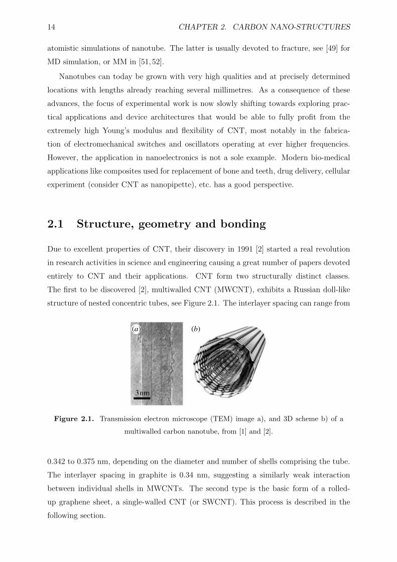
14 CHAPTER 2. CARBON NANO-STRUCTURES
atomistic simulations of nanotube. The latter is usually devoted to fracture, see [49] for
MD simulation, or MM in [51,52].
Nanotubes can today be grown with very high qualities and at precisely determined
locations with lengths already reaching several millimetres. As a consequence of these
advances, the focus of experimental work is now slowly shifting towards exploring prac-
tical applications and device architectures that would be able to fully profit from the
extremely high Young’s modulus and flexibility of CNT, most notably in the fabrica-
tion of electromechanical switches and oscillators operating at ever higher frequencies.
However, the application in nanoelectronics is not a sole example. Modern bio-medical
applications like composites used for replacement of bone and teeth, drug delivery, cellular
experiment (consider CNT as nanopipette), etc. has a good perspective.
2.1 Structure, geometry and bonding
Due to excellent properties of CNT, their discovery in 1991 [2] started a real revolution
in research activities in science and engineering causing a great number of papers devoted
entirely to CNT and their applications. CNT form two structurally distinct classes.
The first to be discovered [2], multiwalled CNT (MWCNT), exhibits a Russian doll-like
structure of nested concentric tubes, see Figure 2.1. The interlayer spacing can range from
Figure 2.1. Transmission electron microscope (TEM) image a), and 3D scheme b) of a
multiwalled carbon nanotube, from [1] and [2].
0.342 to 0.375 nm, depending on the diameter and number of shells comprising the tube.
The interlayer spacing in graphite is 0.34 nm, suggesting a similarly weak interaction
between individual shells in MWCNTs. The second type is the basic form of a rolled-
up graphene sheet, a single-walled CNT (or SWCNT). This process is described in the
following section.
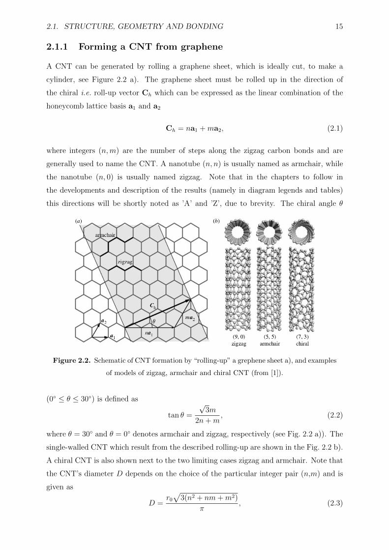
2.1. STRUCTURE, GEOMETRY AND BONDING 15
2.1.1 Forming a CNT from graphene
A CNT can be generated by rolling a graphene sheet, which is ideally cut, to make a
cylinder, see Figure 2.2 a). The graphene sheet must be rolled up in the direction of
the chiral i.e. roll-up vector Ch which can be expressed as the linear combination of the
honeycomb lattice basis a1 and a2
Ch = na1 +ma2, (2.1)
where integers (n,m) are the number of steps along the zigzag carbon bonds and are
generally used to name the CNT. A nanotube (n, n) is usually named as armchair, while
the nanotube (n, 0) is usually named zigzag. Note that in the chapters to follow in
the developments and description of the results (namely in diagram legends and tables)
this directions will be shortly noted as ’A’ and ’Z’, due to brevity. The chiral angle θ
Figure 2.2. Schematic of CNT formation by “rolling-up” a grephene sheet a), and examples
of models of zigzag, armchair and chiral CNT (from [1]).
(0 ≤ θ ≤ 30) is defined as
tan θ =
√3m
2n+m, (2.2)
where θ = 30 and θ = 0 denotes armchair and zigzag, respectively (see Fig. 2.2 a)). The
single-walled CNT which result from the described rolling-up are shown in the Fig. 2.2 b).
A chiral CNT is also shown next to the two limiting cases zigzag and armchair. Note that
the CNT’s diameter D depends on the choice of the particular integer pair (n,m) and is
given as
D =r0
√3(n2 + nm+m2)
π, (2.3)
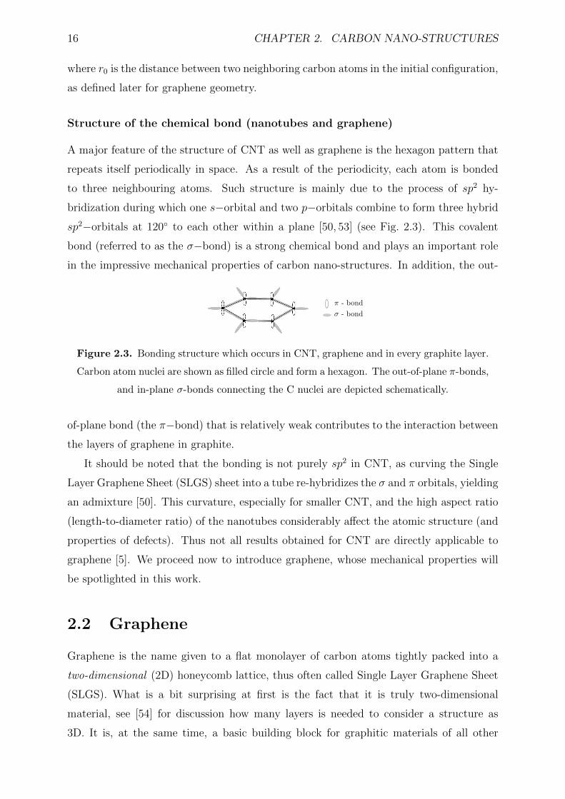
16 CHAPTER 2. CARBON NANO-STRUCTURES
where r0 is the distance between two neighboring carbon atoms in the initial configuration,
as defined later for graphene geometry.
Structure of the chemical bond (nanotubes and graphene)
A major feature of the structure of CNT as well as graphene is the hexagon pattern that
repeats itself periodically in space. As a result of the periodicity, each atom is bonded
to three neighbouring atoms. Such structure is mainly due to the process of sp2 hy-
bridization during which one s−orbital and two p−orbitals combine to form three hybrid
sp2−orbitals at 120 to each other within a plane [50, 53] (see Fig. 2.3). This covalent
bond (referred to as the σ−bond) is a strong chemical bond and plays an important role
in the impressive mechanical properties of carbon nano-structures. In addition, the out-
Figure 2.3. Bonding structure which occurs in CNT, graphene and in every graphite layer.
Carbon atom nuclei are shown as filled circle and form a hexagon. The out-of-plane π-bonds,
and in-plane σ-bonds connecting the C nuclei are depicted schematically.
of-plane bond (the π−bond) that is relatively weak contributes to the interaction between
the layers of graphene in graphite.
It should be noted that the bonding is not purely sp2 in CNT, as curving the Single
Layer Graphene Sheet (SLGS) sheet into a tube re-hybridizes the σ and π orbitals, yielding
an admixture [50]. This curvature, especially for smaller CNT, and the high aspect ratio
(length-to-diameter ratio) of the nanotubes considerably affect the atomic structure (and
properties of defects). Thus not all results obtained for CNT are directly applicable to
graphene [5]. We proceed now to introduce graphene, whose mechanical properties will
be spotlighted in this work.
2.2 Graphene
Graphene is the name given to a flat monolayer of carbon atoms tightly packed into a
two-dimensional (2D) honeycomb lattice, thus often called Single Layer Graphene Sheet
(SLGS). What is a bit surprising at first is the fact that it is truly two-dimensional
material, see [54] for discussion how many layers is needed to consider a structure as
3D. It is, at the same time, a basic building block for graphitic materials of all other
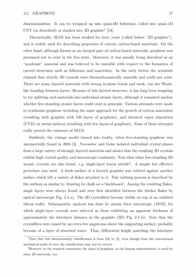
2.2. GRAPHENE 17
dimensionalities. It can be wrapped up into quasi-0D fullerenes, rolled into quasi-1D
CNT (as described) or stacked into 3D graphite1 [54].
Theoretically, SLGS has been studied for sixty years (called before “2D graphite”),
and is widely used for describing properties of various carbon-based materials. On the
other hand, although known as an integral part of carbon-based materials, graphene was
presumed not to exist in the free state. Moreover, it was usually being described as an
“academic” material and was believed to be unstable with respect to the formation of
curved structures such as fullerenes and nanotubes. In the early forties the scientists
claimed that strictly 2D crystals were thermodynamically unstable and could not exist.
There are many layered materials with strong in-plane bonds and weak, van der Waals-
like bonding between layers. Because of this layered structure, it has long been tempting
to try splitting such materials into individual atomic layers, although it remained unclear
whether free-standing atomic layers could exist in principle. Various attempts were made
to synthesize graphene including the same approach for the growth of carbon nanotubes
(resulting with graphite with 100 layers of graphene), and chemical vapor deposition
(CVD) on metal surfaces (resulting with few layers of graphene). None of these attempts
really proved the existence of SLGS.
Suddenly, the vintage model turned into reality, when free-standing graphene was
unexpectedly found in 2004 [3]. Novoselov and Geim isolated individual crystal planes
from a large variety of strongly layered materials and shown that the resulting 2D crystals
exhibit high crystal quality and macroscopic continuity. Note that other free-standing 2D
atomic crystals are also found, e.g. single-layer boron nitride2. A simple but effective
procedure was used. A fresh surface of a layered graphite was rubbed against another
surface which left a variety of flakes attached to it. This rubbing process is described by
the authors as similar to ’drawing by chalk on a blackboard’. Among the resulting flakes,
single layers were always found and were first identified between the thicker flakes by
optical microscope Fig. 2.4 a). The 2D crystallites become visible on top of an oxidized
silicon wafer. Subsequently, analysis was done by atomic force microscopy (AFM), for
which single-layer crystals were selected as those exhibiting an apparent thickness of
approximately the interlayer distance in the graphite (3D) Fig. 2.4 b). Note that the
crystallites were raised by an extra few angstroms above the supporting surface, probably
because of a layer of absorbed water. Thus, differential height matching the interlayer
1Note that this dimensionality classification is from [54] or [3], even though from the conventional
mechanical point of view the classification may not be correct.2However, in the research community the name of graphene, as the famous representative, is used for
other 2D materials, too.
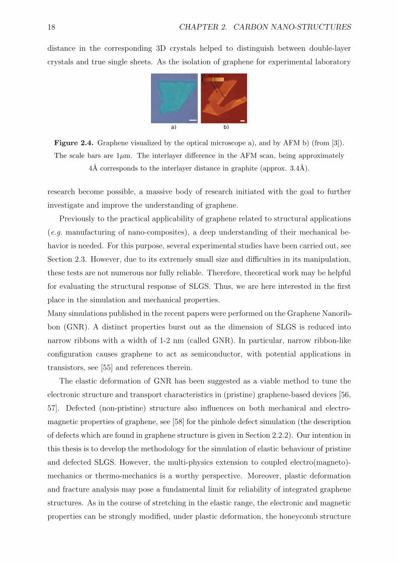
18 CHAPTER 2. CARBON NANO-STRUCTURES
distance in the corresponding 3D crystals helped to distinguish between double-layer
crystals and true single sheets. As the isolation of graphene for experimental laboratory
a) b)
Figure 2.4. Graphene visualized by the optical microscope a), and by AFM b) (from [3]).
The scale bars are 1µm. The interlayer difference in the AFM scan, being approximately
4A corresponds to the interlayer distance in graphite (approx. 3.4A).
research become possible, a massive body of research initiated with the goal to further
investigate and improve the understanding of graphene.
Previously to the practical applicability of graphene related to structural applications
(e.g. manufacturing of nano-composites), a deep understanding of their mechanical be-
havior is needed. For this purpose, several experimental studies have been carried out, see
Section 2.3. However, due to its extremely small size and difficulties in its manipulation,
these tests are not numerous nor fully reliable. Therefore, theoretical work may be helpful
for evaluating the structural response of SLGS. Thus, we are here interested in the first
place in the simulation and mechanical properties.
Many simulations published in the recent papers were performed on the Graphene Nanorib-
bon (GNR). A distinct properties burst out as the dimension of SLGS is reduced into
narrow ribbons with a width of 1-2 nm (called GNR). In particular, narrow ribbon-like
configuration causes graphene to act as semiconductor, with potential applications in
transistors, see [55] and references therein.
The elastic deformation of GNR has been suggested as a viable method to tune the
electronic structure and transport characteristics in (pristine) graphene-based devices [56,
57]. Defected (non-pristine) structure also influences on both mechanical and electro-
magnetic properties of graphene, see [58] for the pinhole defect simulation (the description
of defects which are found in graphene structure is given in Section 2.2.2). Our intention in
this thesis is to develop the methodology for the simulation of elastic behaviour of pristine
and defected SLGS. However, the multi-physics extension to coupled electro(magneto)-
mechanics or thermo-mechanics is a worthy perspective. Moreover, plastic deformation
and fracture analysis may pose a fundamental limit for reliability of integrated graphene
structures. As in the course of stretching in the elastic range, the electronic and magnetic
properties can be strongly modified, under plastic deformation, the honeycomb structure
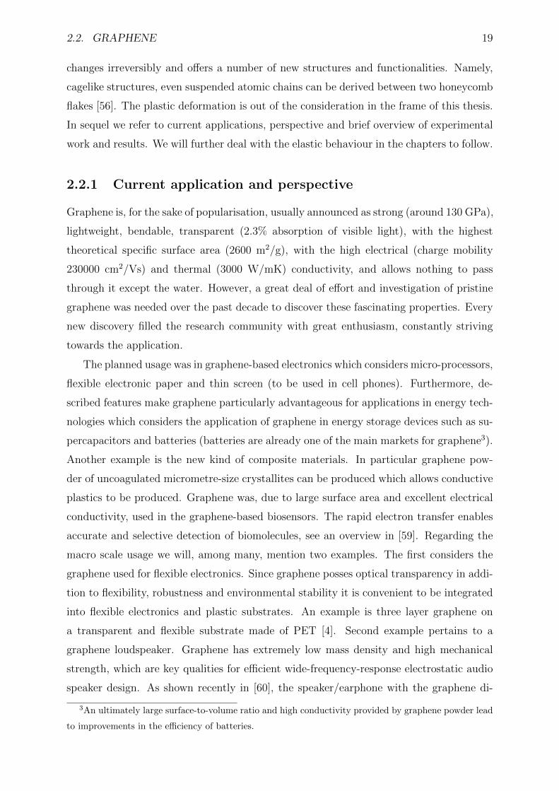
2.2. GRAPHENE 19
changes irreversibly and offers a number of new structures and functionalities. Namely,
cagelike structures, even suspended atomic chains can be derived between two honeycomb
flakes [56]. The plastic deformation is out of the consideration in the frame of this thesis.
In sequel we refer to current applications, perspective and brief overview of experimental
work and results. We will further deal with the elastic behaviour in the chapters to follow.
2.2.1 Current application and perspective
Graphene is, for the sake of popularisation, usually announced as strong (around 130 GPa),
lightweight, bendable, transparent (2.3% absorption of visible light), with the highest
theoretical specific surface area (2600 m2/g), with the high electrical (charge mobility
230000 cm2/Vs) and thermal (3000 W/mK) conductivity, and allows nothing to pass
through it except the water. However, a great deal of effort and investigation of pristine
graphene was needed over the past decade to discover these fascinating properties. Every
new discovery filled the research community with great enthusiasm, constantly striving
towards the application.
The planned usage was in graphene-based electronics which considers micro-processors,
flexible electronic paper and thin screen (to be used in cell phones). Furthermore, de-
scribed features make graphene particularly advantageous for applications in energy tech-
nologies which considers the application of graphene in energy storage devices such as su-
percapacitors and batteries (batteries are already one of the main markets for graphene3).
Another example is the new kind of composite materials. In particular graphene pow-
der of uncoagulated micrometre-size crystallites can be produced which allows conductive
plastics to be produced. Graphene was, due to large surface area and excellent electrical
conductivity, used in the graphene-based biosensors. The rapid electron transfer enables
accurate and selective detection of biomolecules, see an overview in [59]. Regarding the
macro scale usage we will, among many, mention two examples. The first considers the
graphene used for flexible electronics. Since graphene posses optical transparency in addi-
tion to flexibility, robustness and environmental stability it is convenient to be integrated
into flexible electronics and plastic substrates. An example is three layer graphene on
a transparent and flexible substrate made of PET [4]. Second example pertains to a
graphene loudspeaker. Graphene has extremely low mass density and high mechanical
strength, which are key qualities for efficient wide-frequency-response electrostatic audio
speaker design. As shown recently in [60], the speaker/earphone with the graphene di-
3An ultimately large surface-to-volume ratio and high conductivity provided by graphene powder lead
to improvements in the efficiency of batteries.
20 CHAPTER 2. CARBON NANO-STRUCTURES
Figure 2.5. An assembled graphene/PET touch panel showing outstanding flexibility,
from [4].
aphragm has excellent frequency response across the entire audio frequency range and
with performance matching or surpassing commercially available product. Graphene di-
aphragm has ultralow mass and because it is so thin, the speaker does not need to be
artificially damped (unlike commercial devices) to prevent unwanted frequency responses,
but is simply damped by surrounding air. This means that the device uses much less
power than conventional speakers. This is a non-negligible advantage if it were to be
employed in portable devices, such as smartphones, notebooks and tablets.
For the mentioned application the key question pertains to the large scale synthesis of
graphene layers. The key challenge in synthesis and processing of bulk-quantity graphene
sheets is aggregation. Unless well separated from each other, graphene tends to form
irreversible agglomerates or even restack to form graphite through Van der Waals interac-
tions. The prevention of aggregation is essential for graphene sheets because most of their
unique properties are only associated with individual sheets. The common ways to obtain
graphene are exfoliation and cleavage, and chemical vapor deposition (CVD), see [55].
CVD growth appears to be the most promising technique for large-scale production of
graphene films (either in mono- or few-layer form). The growth mechanism of graphene,
on substrates with high carbon solubility such as Co and Ni, is through the diffusion
of the carbon into the metal thin film at the growth temperature, and the subsequent
precipitation of carbon out of the bulk metal to metal surface upon the cooling. Thus, a
typical CVD process involves dissolving carbon into the substrate in the vacuum chamber.
Early tries of graphene growth at ambient pressure using CVD showed single and few
layer graphene (20 µm lateral size) to have a large variation in charge carriers mobility,
thus degradation of properties (namely electrical). The latter is caused by the inhomoge-
2.2. GRAPHENE 21
neous thickness of graphene films and grain boundary scattering inside the films. However,
in recent development [61] it was shown that the quality of graphene (again in terms of
charge carriers mobility) grown by chemical vapour deposition on thin Ni substrate is as
high as mechanically cleaved graphene.
In the next section we will give an overview of the defects that occur in graphene and can
deteriorate it’s properties.
2.2.2 Defected graphene
Due to the imperfection of material production processes, impurities and defects are
always present in crystals (even in nano-crystals). Such lattice imperfections have a
strong influence on the electronic, optical, thermal, and mechanical properties of the
solid. In fact, many of the characteristics of technologically important materials such as
the conductance of semiconductors or the mechanical strength and ductility of metals
are governed by defects. Thus, defects in bulk crystals have been studied extensively for
many decades. Two-dimensional crystals, on the other hand, have been considered only
recently.
The remarkable properties of graphene mentioned above are usually attributed to the
low defect concentration. This nearly pristine state is possible mostly due to the high for-
mation energies of point defects in graphene [5]. Nevertheless, like in other (conventional)
engineering materials, structural defects do exist in graphene and can dramatically alter
its properties. Thus, at first glance, what is true for a 3D material seems to be valid
for graphene as well. The scattering of electron waves at defects influences the electrical
conductivity, and weaker bonds around defects affect the thermal conductivity and reduce
the mechanical strength.
However, graphene structure is unique by being able to reconstruct the atom arrange-
ment in the vicinity of the defect which does not occur in other materials. This feature
comes from the sp2-hybridisation of carbon atoms (shown in Figure 2.3) that allows dif-
ferent number of nearest neighbours, and atom arrangements that are not necessarily
hexagonal. Note that the nonhexagonal rings may either introduce curvature in the sheet
or leave it flat when the arrangement of polygons satisfies certain symmetry rules.
Although many outstanding properties of graphene are due to the inherently low con-
centration of defects, nanoengineering of graphene-based devices for dedicated functions
needs the introduction of structural defects or impurities that allow us, like in conventional
semiconductors, to achieve the desired functionality. For example, Chen et al. [31] have
shown that atom vacancy defects in graphene are magnetic. Takamura et al. [32] suggest
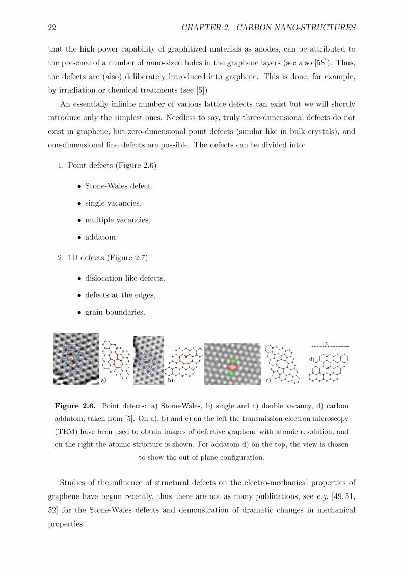
22 CHAPTER 2. CARBON NANO-STRUCTURES
that the high power capability of graphitized materials as anodes, can be attributed to
the presence of a number of nano-sized holes in the graphene layers (see also [58]). Thus,
the defects are (also) deliberately introduced into graphene. This is done, for example,
by irradiation or chemical treatments (see [5])
An essentially infinite number of various lattice defects can exist but we will shortly
introduce only the simplest ones. Needless to say, truly three-dimensional defects do not
exist in graphene, but zero-dimensional point defects (similar like in bulk crystals), and
one-dimensional line defects are possible. The defects can be divided into:
1. Point defects (Figure 2.6)
• Stone-Wales defect,
• single vacancies,
• multiple vacancies,
• addatom.
2. 1D defects (Figure 2.7)
• dislocation-like defects,
• defects at the edges,
• grain boundaries.
a) b) c)
d)
Figure 2.6. Point defects: a) Stone-Wales, b) single and c) double vacancy, d) carbon
addatom, taken from [5]. On a), b) and c) on the left the transmission electron microscopy
(TEM) have been used to obtain images of defective graphene with atomic resolution, and
on the right the atomic structure is shown. For addatom d) on the top, the view is chosen
to show the out of plane configuration.
Studies of the influence of structural defects on the electro-mechanical properties of
graphene have begun recently, thus there are not as many publications, see e.g. [49, 51,
52] for the Stone-Wales defects and demonstration of dramatic changes in mechanical
properties.
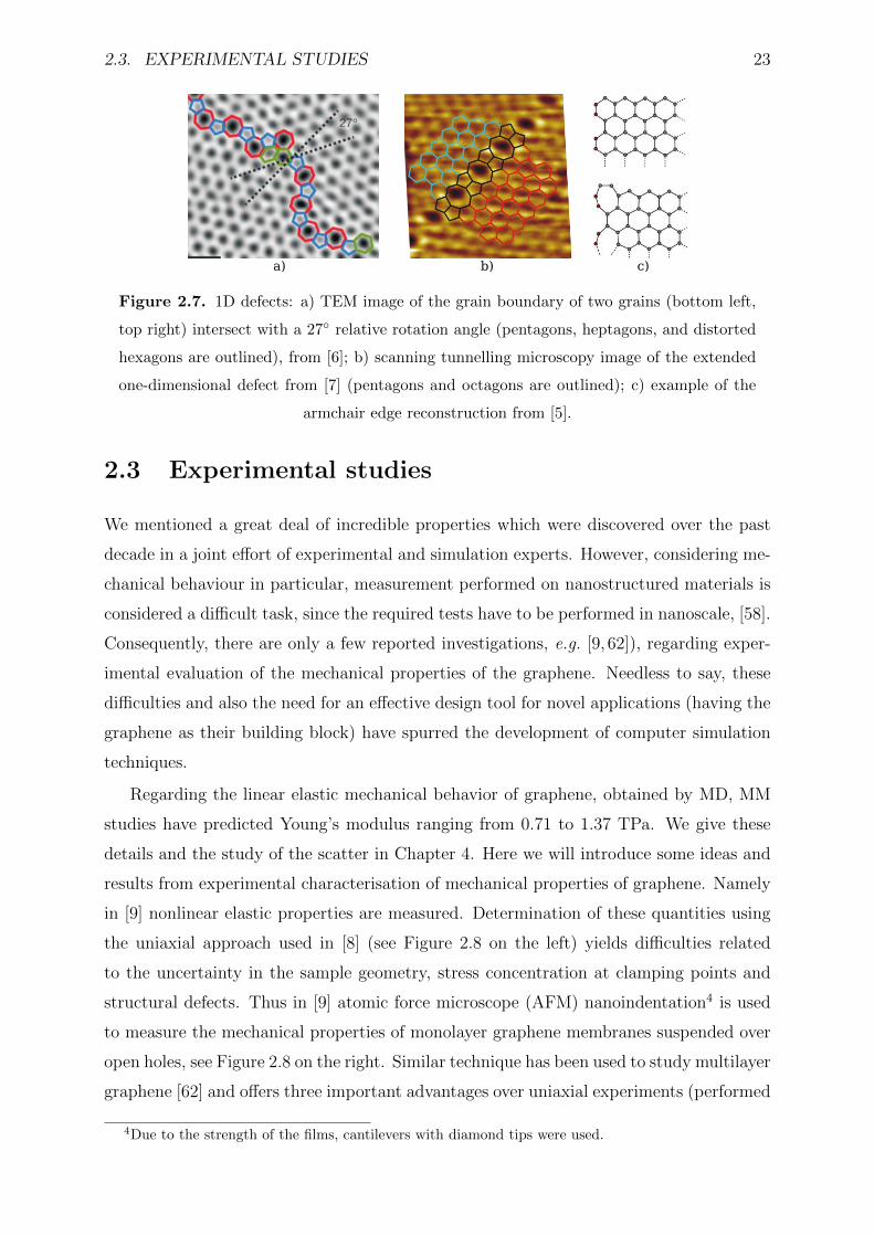
2.3. EXPERIMENTAL STUDIES 23
a) b) c)
Figure 2.7. 1D defects: a) TEM image of the grain boundary of two grains (bottom left,
top right) intersect with a 27 relative rotation angle (pentagons, heptagons, and distorted
hexagons are outlined), from [6]; b) scanning tunnelling microscopy image of the extended
one-dimensional defect from [7] (pentagons and octagons are outlined); c) example of the
armchair edge reconstruction from [5].
2.3 Experimental studies
We mentioned a great deal of incredible properties which were discovered over the past
decade in a joint effort of experimental and simulation experts. However, considering me-
chanical behaviour in particular, measurement performed on nanostructured materials is
considered a difficult task, since the required tests have to be performed in nanoscale, [58].
Consequently, there are only a few reported investigations, e.g. [9, 62]), regarding exper-
imental evaluation of the mechanical properties of the graphene. Needless to say, these
difficulties and also the need for an effective design tool for novel applications (having the
graphene as their building block) have spurred the development of computer simulation
techniques.
Regarding the linear elastic mechanical behavior of graphene, obtained by MD, MM
studies have predicted Young’s modulus ranging from 0.71 to 1.37 TPa. We give these
details and the study of the scatter in Chapter 4. Here we will introduce some ideas and
results from experimental characterisation of mechanical properties of graphene. Namely
in [9] nonlinear elastic properties are measured. Determination of these quantities using
the uniaxial approach used in [8] (see Figure 2.8 on the left) yields difficulties related
to the uncertainty in the sample geometry, stress concentration at clamping points and
structural defects. Thus in [9] atomic force microscope (AFM) nanoindentation4 is used
to measure the mechanical properties of monolayer graphene membranes suspended over
open holes, see Figure 2.8 on the right. Similar technique has been used to study multilayer
graphene [62] and offers three important advantages over uniaxial experiments (performed
4Due to the strength of the films, cantilevers with diamond tips were used.
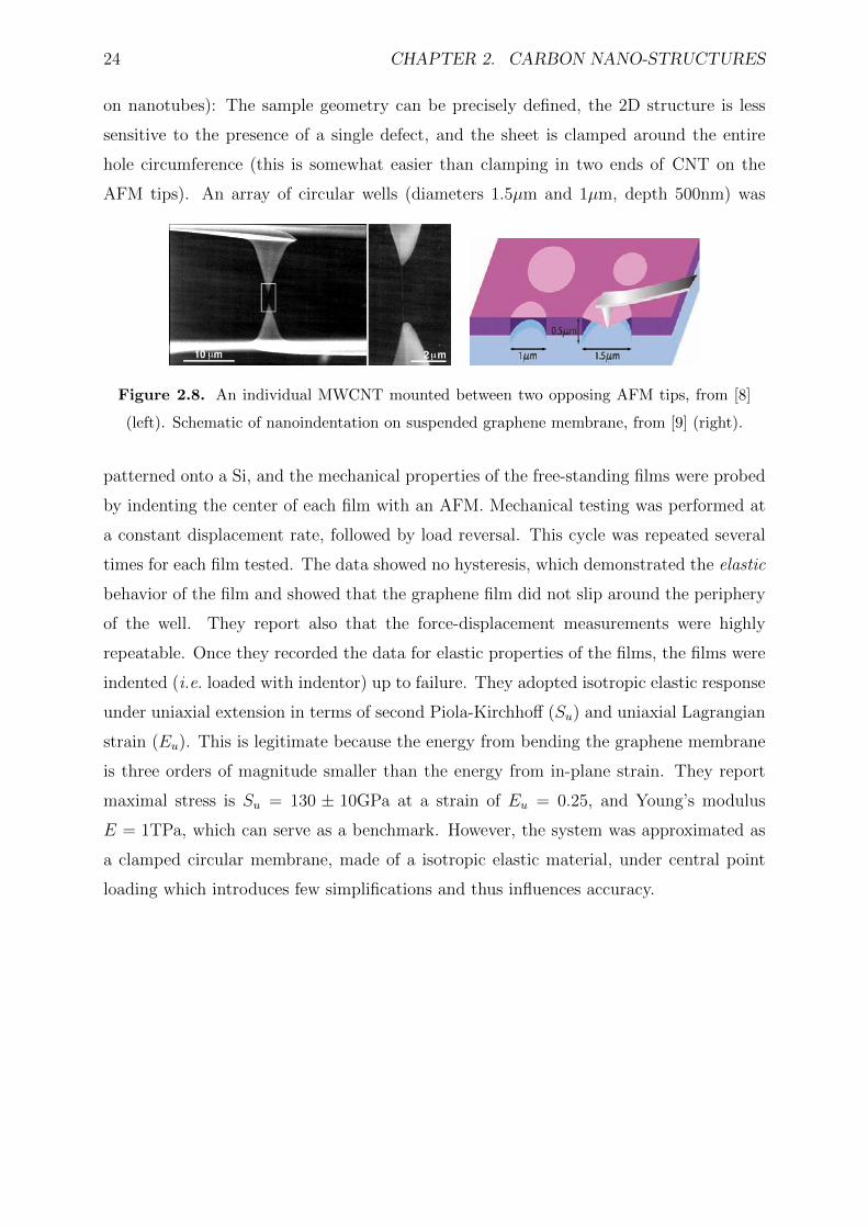
24 CHAPTER 2. CARBON NANO-STRUCTURES
on nanotubes): The sample geometry can be precisely defined, the 2D structure is less
sensitive to the presence of a single defect, and the sheet is clamped around the entire
hole circumference (this is somewhat easier than clamping in two ends of CNT on the
AFM tips). An array of circular wells (diameters 1.5µm and 1µm, depth 500nm) was
Figure 2.8. An individual MWCNT mounted between two opposing AFM tips, from [8]
(left). Schematic of nanoindentation on suspended graphene membrane, from [9] (right).
patterned onto a Si, and the mechanical properties of the free-standing films were probed
by indenting the center of each film with an AFM. Mechanical testing was performed at
a constant displacement rate, followed by load reversal. This cycle was repeated several
times for each film tested. The data showed no hysteresis, which demonstrated the elastic
behavior of the film and showed that the graphene film did not slip around the periphery
of the well. They report also that the force-displacement measurements were highly
repeatable. Once they recorded the data for elastic properties of the films, the films were
indented (i.e. loaded with indentor) up to failure. They adopted isotropic elastic response
under uniaxial extension in terms of second Piola-Kirchhoff (Su) and uniaxial Lagrangian
strain (Eu). This is legitimate because the energy from bending the graphene membrane
is three orders of magnitude smaller than the energy from in-plane strain. They report
maximal stress is Su = 130 ± 10GPa at a strain of Eu = 0.25, and Young’s modulus
E = 1TPa, which can serve as a benchmark. However, the system was approximated as
a clamped circular membrane, made of a isotropic elastic material, under central point
loading which introduces few simplifications and thus influences accuracy.
Chapter 3Atomistic modeling
In this chapter we introduce the atomistic material modelling, we give the essential ideas
and review the related literature. Furthermore, we present a brief overview of the gov-
erning equations, and the interatomic potentials used for atomistic modelling. Note that
these potentials come from the group of classical potentials, as described in the Introduc-
tion. In the literature both terms ’atomistic’ and ’molecular’ modeling are equally used.
Herein we use term ’atomistic’, however, we also use the common name for the simulation
methods named molecular dynamics, or molecular mechanics.
3.1 Atomistic model problem
Computer simulations used to determine the mechanical properties of complex atomic
structures do not often consider the quantum mechanical effects at the subatomic level.
The most frequent starting point in atomic simulations is MD or MM, neglecting the
inertia effect. Both of these methods are based on the assumption that atoms are the
smallest unit needed to be modelled. This enables, furthermore, to study the discrete
atomic structure as a multi-particle system. The way the atoms interaction is described
depends on the choice of the interatomic potential.
We focus in this work upon the MM neglecting both the dynamic effects and the
thermal effects, used for quasi-static loading applications with the assumption of the zero
Kelvin temperature. The equilibrium configuration of graphene corresponds to a state of
minimum energy of the particle system. It is assumed here that the initial configuration
is at equilibrium.
We consider a domain Ωa in a 3-dimensional Euclidian space R3, which is occupied
by N atoms placed within graphene microstructure. Let Ri and ri denote, respectively,
the position vectors in the reference and the current configurations of atom i, where
25
26 CHAPTER 3. ATOMISTIC MODELING
i = 1, . . . , N . The corresponding displacement vector of atom i is given by di = ri −Ri.
Thus the displacement of the atoms is conveniently represented in compact form by means
of vector d = [d1,d2, . . . ,dN ] from the space Va = d ∈ R3×N. The boundary conditions
ought to be defined atom-wise, such that either the displacement di or the external point
force fi takes an imposed value. These conditions are imposed in quasi-static manner,
with the corresponding incremental sequence.
The total energy Eatot of the atomic microstructure is given by
Eatot = U(r1, . . . , rN)−
N∑i
fi · di, (3.1)
where U denotes the energy stored in the atomic bonds, and the second term on the right-
hand side represents the external energy Eext. The state of equilibrium of the atomistic
system corresponds to the minimum of the total energy. The necessary condition of the
energy minimum requires that the variation of the total energy equals zero, which can be
written as
δEatot =
N∑i
(∂U
∂ri− fi
)· δri = 0. (3.2)
In the above equation δri represents the kinematically admissible virtual movement from
the set of Va0 ⊂ R3×N , vanishing on the Dirichlet boundary. Linearising (3.2) and writing
the result in matrix notation leads to
K(k)∆d(k) = F(k), (3.3)
where ∆d(k) is displacement increment corresponding to the k-th load increment, whereas
K(k) and F(k) are the tangent stiffness and residual vector, respectively. The latter can
be explicitly defined as
Kij =∂2U
∂ri∂rj, Fi =
∂U
∂ri− fi. (3.4)
An incremental-iterative solver is needed to solve system in (3.3) due to the nonlin-
ear nature of the interatomic potential (described in sequel) and geometrically nonlinear
kinematics. For each load increment several Newton iterations are performed until con-
vergence criteria are met in terms of energy test, which checks both the residual force and
incremental displacement (e.g. [10]). In Appendix A Newton’s incremental-iterative pro-
cedure is described in more detail. At each iteration (k) the atomic positions are updated
as follows
r(k+1)i = r
(k)i + ∆d(k). (3.5)
The initial iteration (k) = 0 starts at the initial configuration of the atomic system, with
the position vector r(0)i = Ri. The procedure is terminated when the convergence is
achieved for the last load increment.
3.2. INTERATOMIC POTENTIAL 27
What needs to be defined next is the energetics of the atomic system. The latter is
defined with the interatomic potential U . In sequel we first give the general insight in the
classical interatomic potentials and their structure. Next we present specific some specific
forms.
3.2 Interatomic potential
If the atomistic modeling is used as a testing ground for the energetics of the system, the
simplest generic form of the interaction model is considered. When the goal is to repre-
sent the quantitative predictions for specific material, the potential function (U) driving
the atomistic system can take complicated form. As described in the Introduction, the
nature of these interactions is governed by quantum effects taking place at the subatomic
level. The latter is really responsible for chemical properties such as valence and bond
energy [16, 18, 21]. However, quantum mechanics-based description of atomic interaction
is not discussed in this work, emphasis is rather on the empirical interaction models that
can be derived as the result of such computations, i.e. from experimental observations.
Classical potential is designed to account for the quantum effects in the average sense. Let
U(ri, relj ) denote the microscopic energy function that explicitly account for each atom i
with coordinates ri, and each electronic degree of freedom relj1. Then the classical poten-
tial (used in this work) pertain to the approximation which considers that the electronic
degrees of freedom are completely removed, which can be written as
U(ri, relj )→ Uapprox(ri). (3.6)
Many different expressions U(ri) can be fit to closely reproduce the energy predicted
from quantum mechanics methods, while retaining computational efficiency [13,63]. There
is no single, universal approach that is suitable for all materials and for all different
phenomena of material behavior. The choice of the interatomic potential depends very
strongly on both the particular application and the material.
3.2.1 Structure of the potential
The general structure of the potential energy function (approximate potential surface) for
a system of N atoms is
U(r1, r2, . . . , rN) =N∑i
V1(ri) +N∑i,j>i
V2(ri, rj) +N∑
i,j>i,k>i
V3(ri, rj, rk) + · · · , (3.7)
1The electronic degrees of freedom are accounted explicitly in tight-binding models, see [15].
28 CHAPTER 3. ATOMISTIC MODELING
where the function Vm, ∀m = 1, 2, . . . is the m-body potential and ri is the position vector
of the atom i in current configuration. The first term of the right hand side of equation
(3.7) indicates the effect of an external force field on the system where it is immersed,
such as gravitational or electrostatic. This term is usually ignored in practice, [16]. The
second term V2 shows pair-wise interaction depending only on one variable the atom pair
separation given as rij. Thus this term is usually denoted as Vij or Vp as described in
sequel. The three-body term involves energy that characterizes angle-dependent forces,
whereas four-body term includes torsion effects. m-body potential terms for m > 2
are usually called multi-body potentials. Apart from V2, which depends on only one
independent variable, each further term has 3m− 6 variables. Thus, V3 depends on 3 and
V4 on 6 variables.
The simplest form, used often for practical reasons, is when the sum in (3.7) is trun-
cated after second term resulting with the pair-wise potential.
3.2.2 Pair-wise potentials
The total energy of the system in pair potentials is given by summing the energy of all
atomic bonds over all N particles in the system
U =1
2
N∑i 6=j=1
N∑j=1
V2(rij). (3.8)
Note the factor 1/2 which accounts for the double counting of atomic bonds. The latter
equation is more conveniently written as
U =N−1∑i=1
N∑j>i
V2(rij), (3.9)
where the sum directly corresponds to the loop in the code. On the other hand, the total
energy of the system of atoms can be represented as the sum of atom energies. That is,
the energy is given on per atom basis (not per bond) as
U =N∑i=1
Ei =1
2
∑i,j 6=i
Vij, (3.10)
where Ei is the energy of atom i. The pair potential usually decays very fast with the
increase of distance between atom pair rij (see Figure 3.1). In general, we say that the
function decays rapidly with the distance if it decays faster in rij then 1/rdij, where d
is the dimension of the problem [18]. In order to save computational time in the case
of rapidly decaying potential, we can neglect all the contribution in the sum (3.8) that
3.2. INTERATOMIC POTENTIAL 29
are smaller than certain threshold. This value is usually called cut-off distance or cut-off
radius, Rc (see e.g. [63, 64]). Taking into account the interactions of each current atom i
with all the others in the system, the computational demand is (N2 − N)/2 operations.
This is very expensive even for systems with a smaller number of particles. Therefore, in
practical simulations the introduction of a cut-off radius allows us to reduce significantly
the computational effort. The main idea is to replace the sum over all the atoms by the
interaction only with its nearest neighbours which are inside the cut-off radius. The latter
reduces the number of terms to nN/2, with n being the number of atoms into the cut-off
radius. The truncated potential can be formally written as follows
V (rij) =
V (rij) rij ≤ Rc,
0 rij > Rc.(3.11)
In others words, if the interatomic distances exceeds the cut-off, the interactions are simply
set to zero. However, this produces a break in the continuity of the potential function at
the cut-off separation, causing a small step in the energy function as atoms move in and
out of the cut-off. This can cause the fluctuations in the energy during the simulation
which perturbs the conservation of energy in the system. This truncation may be applied
to any potential energy function, i.e. for all the examples presented in sequel, but the
value of cut-off radius have to be chosen with care.
One of the best known interatomic potentials is the Lennard-Jones (LJ), or yet called
6-12 potential. The potential energy function for the LJ potential is expressed as
V LJ2 (rij) = 4ε
((σ
rij
)12
−(σ
rij
)6), (3.12)
where ε and σ are constants chosen to fit material properties. There is no relation to
continuum stress and strain (see Fig. 3.1). The parameter ε stands for the pair well
depth, while σ parametrizes the zero crossing of the potential. Note that the equilibrium
bond separation is related to parameter σ with rij,0 = σ21/6. The celebrated LJ potential
is in fact a particular case of Mie potential, proposed in 1903 [65], which can be written
as
V2(rij) = − Arnij
+B
rmij, (3.13)
with the values of n = 6 and m = 12. Mie’s potential was the first one including both a
repulsive and an attractive part. Term 1/r12ij in LJ is meant to model the repulsion between
atoms as they approach each other, and is motivated by the Pauli principle in chemistry.
The Pauli principle implies that as the electron clouds of the atoms begin to overlap, the
system energy increases dramatically because two interacting electrons cannot occupy the
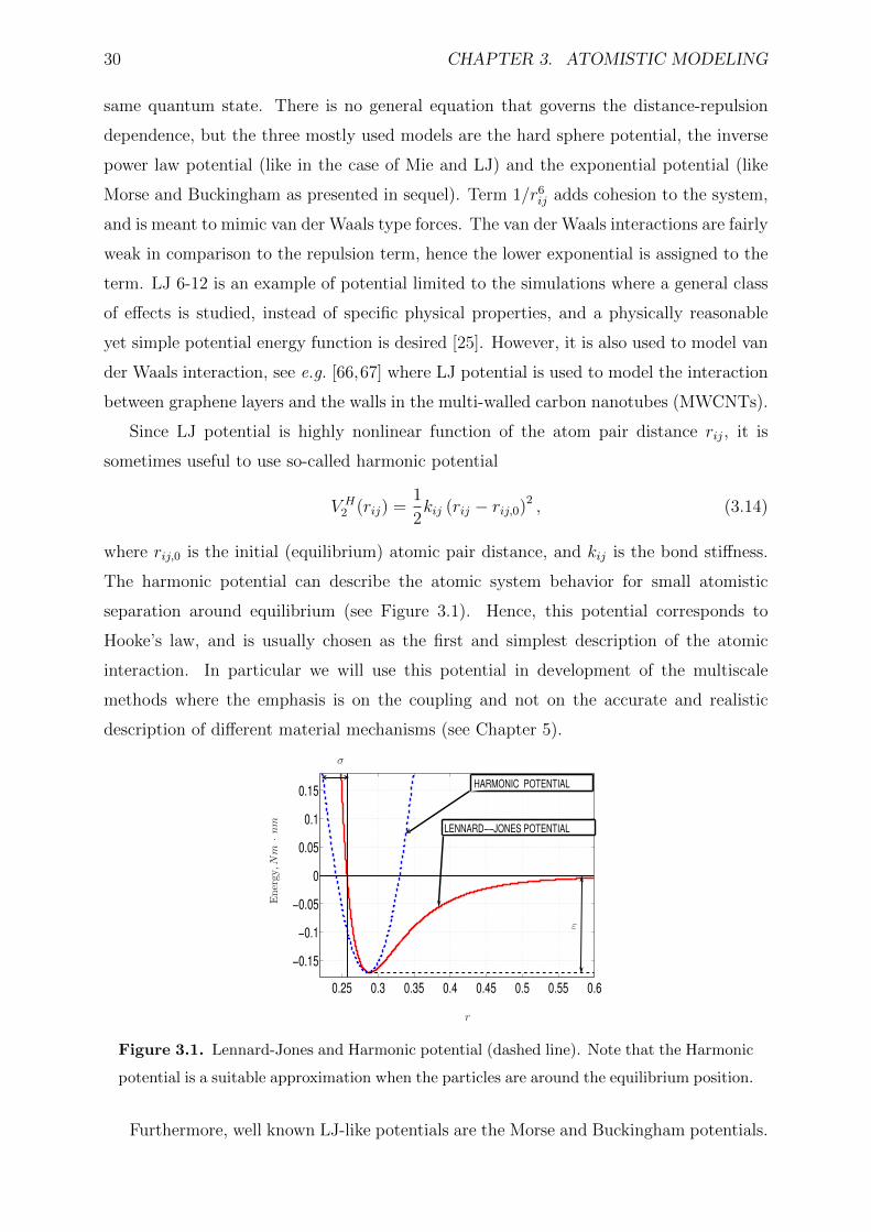
30 CHAPTER 3. ATOMISTIC MODELING
same quantum state. There is no general equation that governs the distance-repulsion
dependence, but the three mostly used models are the hard sphere potential, the inverse
power law potential (like in the case of Mie and LJ) and the exponential potential (like
Morse and Buckingham as presented in sequel). Term 1/r6ij adds cohesion to the system,
and is meant to mimic van der Waals type forces. The van der Waals interactions are fairly
weak in comparison to the repulsion term, hence the lower exponential is assigned to the
term. LJ 6-12 is an example of potential limited to the simulations where a general class
of effects is studied, instead of specific physical properties, and a physically reasonable
yet simple potential energy function is desired [25]. However, it is also used to model van
der Waals interaction, see e.g. [66,67] where LJ potential is used to model the interaction
between graphene layers and the walls in the multi-walled carbon nanotubes (MWCNTs).
Since LJ potential is highly nonlinear function of the atom pair distance rij, it is
sometimes useful to use so-called harmonic potential
V H2 (rij) =
1
2kij (rij − rij,0)2 , (3.14)
where rij,0 is the initial (equilibrium) atomic pair distance, and kij is the bond stiffness.
The harmonic potential can describe the atomic system behavior for small atomistic
separation around equilibrium (see Figure 3.1). Hence, this potential corresponds to
Hooke’s law, and is usually chosen as the first and simplest description of the atomic
interaction. In particular we will use this potential in development of the multiscale
methods where the emphasis is on the coupling and not on the accurate and realistic
description of different material mechanisms (see Chapter 5).
Figure 3.1. Lennard-Jones and Harmonic potential (dashed line). Note that the Harmonic
potential is a suitable approximation when the particles are around the equilibrium position.
Furthermore, well known LJ-like potentials are the Morse and Buckingham potentials.
3.2. INTERATOMIC POTENTIAL 31
The Morse potential consists of the exponential repulsion and attraction and three ad-
justable parameters. It is originally designed for covalent bond which is strongly space
oriented and a description of radial stretching is not sufficient to describe it. The Morse
potential [68] is computationally more expensive than the LJ potential due to the expo-
nential model of repulsion and attraction but it models interaction in a more realistic way.
It can be given in the form
V M2 = ε
(e
2α(1− rr0
) − 2eα(1− r
r0)), (3.15)
where we omitted the indices ij in the current and initial separation r and r0. The
parameters of the potential are ε, α, and r0. We will use the modified type of this
potential throughout this work for graphene modeling, thus we give a detailed overview
in Section 3.2.4. The Buckingham potential consists of more physical exponential Born-
Meyer repulsion and the van der Waals attraction in the following form
V B2 = Ae
α(1− rr0
) − B
r6, (3.16)
where A and B are constants. Since the exponent becomes smaller than the inverse
power law at very small bond separations, the potential drops rapidly to minus infinity.
The latter unphysical effect is often referred to as Buckingham catastrophe. In order
to bring the Buckingham and the LJ potentials to a common equilibrium distance r0,
and to a common well depth ε, the relation between the LJ parameters ε and σ and the
Buckingham parameters A, B and α is as follows
A =1
2− ε, B = σ6, α =
312− ε. (3.17)
In conclusion of this section we note that the reduction of the total energy caused
by the truncation of the sum in (3.7) after second term leads to discrepancies between
theory and experiment. These discrepancies can be observed in terms of: the single bond
strength being independent of the next neighbours, the vacancy formation energy which
is always overestimated by pair potentials, the prediction of the inward relaxation of the
outer layer of atoms at the surface yields incorrect results, etc. Thus, in sequel we intro-
duce the improvement of classical pairwise potentials.
3.2.3 Beyond pair-wise potentials
Mentioned deficiency of pair potentials have led to the development of more complex
potentials. Such potentials incorporate local environment of an atom into the potential
32 CHAPTER 3. ATOMISTIC MODELING
through many-body effects to produce a more realistic description of the atomic interac-
tions. Thus, we still consider the pair of atoms, while the positions of the several neig-
bouring atoms are taken into account. These potentials are typically used in simulations
of solids and complex molecular structures. There is a number of many-body potentials
for modelling of covalent bonds which have been developed in recent decades. Potentials
which also fit in this group are Finnis and Sinclair potential, and Embedded atom method
(EAM) (see [69–71]), however, they are both used to simulate microcracks and structural
changes in metallic materials. Thus, we will discuss more on the Stillinger-Weber, Bren-
ner and latter focus on the modified Morse potentials used to model hydrocarbon bonds,
i.e. covalent systems.
Stillinger-Weber potential
One of the traditional formulations to express many-body interactions have been suggested
by Stillinger and Weber [72]. It is used mostly to describe the behaviour of Si, i.e. the
materials with a low coordination number and strong directed bonds. This potential is
based on a two-body and a three-body term
U =∑i,j
V2(rij) +∑i,j,k
V3(ri, rj, rk), (3.18)
where the pair potential is taken to be from the family of the inverse power law and
the exponential potential (as discussed in the previous section), while the tree-body term
provides the dependence of the total energy on the bond angle. The angular term has the
form
V3(ri, rj, rk) = h(rij, rik, θjik) + h(rji, rjk, θijk) + h(rki, rkj, θikj), (3.19)
with
h(rij, rik, θjik) = λe
(γ
rij−Rc
)e
(γ
rik−Rc
) [cos θijk +
1
3
]. (3.20)
In the above equations θjik is the angle formed by the i − j bond and the i − k bonds,
λ and γ are tunable parameters, while Rc denotes the cut-off distance. The latter shows
that the same cut-off advantage can be extended to three-body terms [72]. The main
drawback of this description is that it cannot be applied for non-tetrahedral crystals.
Tersoff-Brenner potential
A further celebrated potential, which should be mentioned in this section is the Tersoff
potential [73]. Tersoff proposed an empirical potential that enables to calculate the struc-
ture and energetics of complex covalently bonded systems, with the focus on silicon. This
3.2. INTERATOMIC POTENTIAL 33
potential is further developed for hydrocarbons by D. W. Brenner [74], thus the poten-
tial is often referred to as Tersoff-Brenner (TB). The form of the potential is motivated
by intuitive ideas about the dependence of bond order upon local environment, i.e. it
incorporates the structural chemistry of covalent systems. The total potential energy is
calculated as for the simple pair potential, see equations (3.8) or (3.10). However, Vij is
here given as
Vij = VR(rij)−BijVA(rij), (3.21)
for atoms i and j. VR and VA are exponential, Morse-like repulsive and attractive pair
terms, respectively, given by
VR(rij) =De
S − 1e−√
2Sβ(rij−rij,0)fc(rij), (3.22)
VA(rij) =De
S − 1e−√
2/Sβ(rij−rij,0)fc(rij). (3.23)
The parameters De (well depth), S, β, and rij,0 are determined from the known physical
properties of carbon (i.e. carbon allotropes). The function fc is merely a smooth cut-off
function to limit the range of the potential, and is given by
fc(rij) =
1 rij < R1,
12− 1
2sin( πr−R1
R2−R1) R1 < rij < R2,
0 rij > R2.
(3.24)
For the graphene the cut-off is taken to be R2 = 0.2 nm and R1 = 0.17 nm to include
only the first-neighbour shell. The function Bij implicitly incorporates the bond order
and depends on local environment, rather than to have three body terms
Bij =
[1 +
∑k 6=i,j
G(θijk)fc(rik
]−δ, (3.25)
where the function G is given by [75]
G(θ) = a0
[1 +
c20
d20
− c20
d20 + (1 + cos θ)2
]. (3.26)
The numerical values of the parameters in (3.22), (3.23), (3.24), (3.25) and (3.26) are
as follows [74] De = 6.0 eV, S = 1.22, β = 21 nm−1, rij,0 = 0.139 nm, δ = 0.5, a0 =
0.00020813, c0 = 330, d0 = 3.5. The improved, second generation of the TB potential,
so called reactive empirical bond order (REBO) potential for covalent bond breaking and
forming, is developed in [76].
The TB potential has a broader application field than the SW potential, and the unique
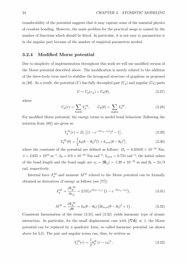
34 CHAPTER 3. ATOMISTIC MODELING
transferability of the potential suggests that it may capture some of the essential physics
of covalent bonding. However, the main problem for the practical usage is caused by the
number of functions which should be fitted. In particular, it is not easy to parametrize it
in the angular part because of the number of empirical parameters needed.
3.2.4 Modified Morse potential
Due to simplicity of implementation throughout this work we will use modified version of
the Morse potential described above. The modification is merely related to the addition
of the three-body term used to stabilize the hexagonal structure of graphene as proposed
in [49]. As a result, the potential (U) has fully decoupled pair (Up) and angular (Uθ) parts
U = Up(rij) + Uθ(θ), (3.27)
where
Up(r) =∑bonds
V Mp , Uθ(θ) =
∑angles
V Mθ . (3.28)
For modified Morse potential, the energy terms to model bond behaviour (following the
notation from [49]) are given as
V Mp (r) = De
[(1− e−β(rij−r0))2 − 1
], (3.29)
V Mθ (θ) =
1
2kθ(θ − θ0)2[1 + ksext(θ − θ0)4], (3.30)
where the constants of the potential are defined as follows: De = 6.03105 × 10⁻¹⁹ Nm,
β = 2.625× 10¹⁰ m−1, kθ = 0.9× 10⁻¹⁸ Nm rad−2, ksext = 0.754 rad−4; the initial values
of the bond length and the bond angle are r0 = |Rij| = 1.39 × 10⁻¹⁰ m and θ0 = 2π/3
rad, respectively.
Internal force FMp and moment MM related to the Morse potential can be formally
obtained as derivatives of energy as follows (see [77])
FMp =
∂V Mp
∂rij= 2βDee
β(r0−rij)(1− e−β(rij−r0)
), (3.31)
MM =∂V M
θ
∂θ= kθ(θ − θ0)
(3ksext(θ − θ0)4 + 1
). (3.32)
Consistent linearisation of the terms (3.31) and (3.32) yields harmonic type of atomic
interaction. In particular, for the small displacement case with ‖∇d‖ 1, the Morse
potential can be replaced by a quadratic form, so called harmonic potential (as shown
above for LJ). The pair and angular terms can, thus, be written as
V Hp (r) =
1
2kHp (r − r0)2 , (3.33)
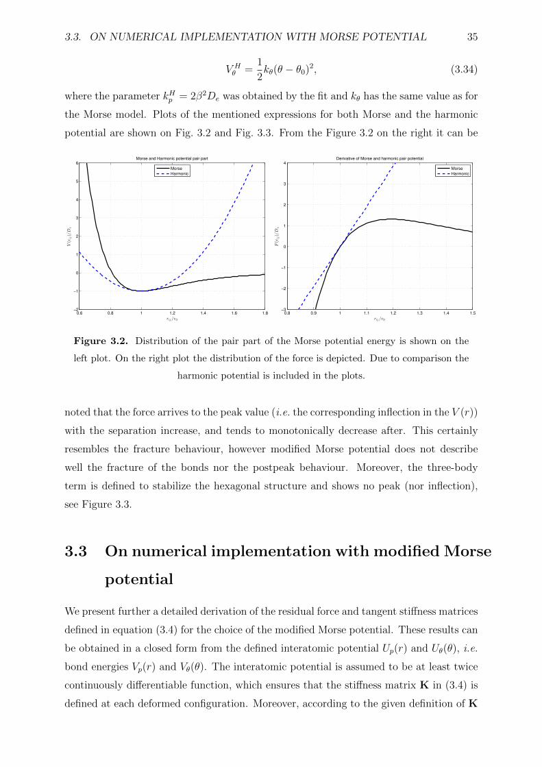
3.3. ON NUMERICAL IMPLEMENTATION WITH MORSE POTENTIAL 35
V Hθ =
1
2kθ(θ − θ0)2, (3.34)
where the parameter kHp = 2β2De was obtained by the fit and kθ has the same value as for
the Morse model. Plots of the mentioned expressions for both Morse and the harmonic
potential are shown on Fig. 3.2 and Fig. 3.3. From the Figure 3.2 on the right it can be
0.6 0.8 1 1.2 1.4 1.6 1.8−2
−1
0
1
2
3
4
5
6Morse and Harmonic potential pair part
rij/r0
V(r
ij)/D
e
Morse
Harmonic
0.8 0.9 1 1.1 1.2 1.3 1.4 1.5−3
−2
−1
0
1
2
3
4Derivative of Morse and harmonic pair potential
rij/r0
F(r
ij)/D
e
Morse
Harmonic
Figure 3.2. Distribution of the pair part of the Morse potential energy is shown on the
left plot. On the right plot the distribution of the force is depicted. Due to comparison the
harmonic potential is included in the plots.
noted that the force arrives to the peak value (i.e. the corresponding inflection in the V (r))
with the separation increase, and tends to monotonically decrease after. This certainly
resembles the fracture behaviour, however modified Morse potential does not describe
well the fracture of the bonds nor the postpeak behaviour. Moreover, the three-body
term is defined to stabilize the hexagonal structure and shows no peak (nor inflection),
see Figure 3.3.
3.3 On numerical implementation with modified Morse
potential
We present further a detailed derivation of the residual force and tangent stiffness matrices
defined in equation (3.4) for the choice of the modified Morse potential. These results can
be obtained in a closed form from the defined interatomic potential Up(r) and Uθ(θ), i.e.
bond energies Vp(r) and Vθ(θ). The interatomic potential is assumed to be at least twice
continuously differentiable function, which ensures that the stiffness matrix K in (3.4) is
defined at each deformed configuration. Moreover, according to the given definition of K
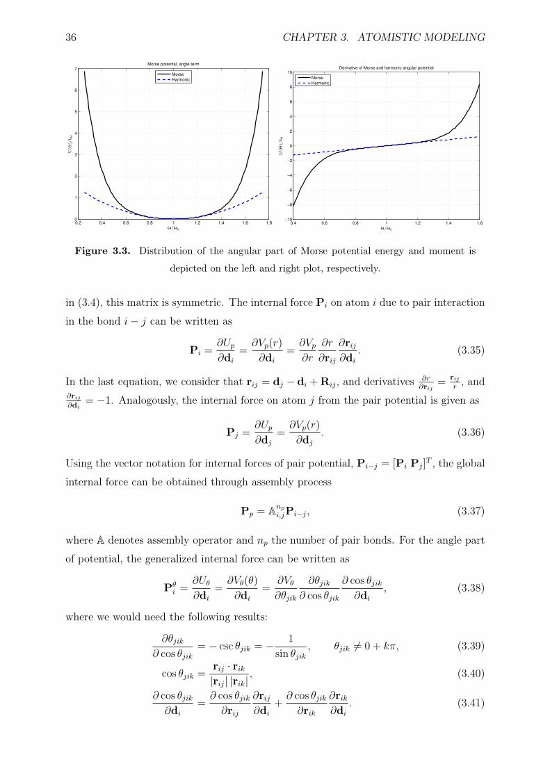
36 CHAPTER 3. ATOMISTIC MODELING
0.2 0.4 0.6 0.8 1 1.2 1.4 1.6 1.80
1
2
3
4
5
6
7Morse potential, angle term
Θ/Θ0
V(Θ
)/kΘ
Morse
Harmonic
0.4 0.6 0.8 1 1.2 1.4 1.6−10
−8
−6
−4
−2
0
2
4
6
8
10Derivative of Morse and harmonic angular potential
Θ/Θ0
M(Θ
)/kΘ
Morse
Harmonic
Figure 3.3. Distribution of the angular part of Morse potential energy and moment is
depicted on the left and right plot, respectively.
in (3.4), this matrix is symmetric. The internal force Pi on atom i due to pair interaction
in the bond i− j can be written as
Pi =∂Up∂di
=∂Vp(r)
∂di=∂Vp∂r
∂r
∂rij
∂rij∂di
. (3.35)
In the last equation, we consider that rij = dj − di + Rij, and derivatives ∂r∂rij
=rijr
, and∂rij∂di
= −1. Analogously, the internal force on atom j from the pair potential is given as
Pj =∂Up∂dj
=∂Vp(r)
∂dj. (3.36)
Using the vector notation for internal forces of pair potential, Pi−j = [Pi Pj]T , the global
internal force can be obtained through assembly process
Pp = Anpi,jPi−j, (3.37)
where A denotes assembly operator and np the number of pair bonds. For the angle part
of potential, the generalized internal force can be written as
Pθi =
∂Uθ∂di
=∂Vθ(θ)
∂di=
∂Vθ∂θjik
∂θjik∂ cos θjik
∂ cos θjik∂di
, (3.38)
where we would need the following results:
∂θjik∂ cos θjik
= − csc θjik = − 1
sin θjik, θjik 6= 0 + kπ, (3.39)
cos θjik =rij · rik|rij| |rik|
, (3.40)
∂ cos θjik∂di
=∂ cos θjik∂rij
∂rij∂di
+∂ cos θjik∂rik
∂rik∂di
. (3.41)
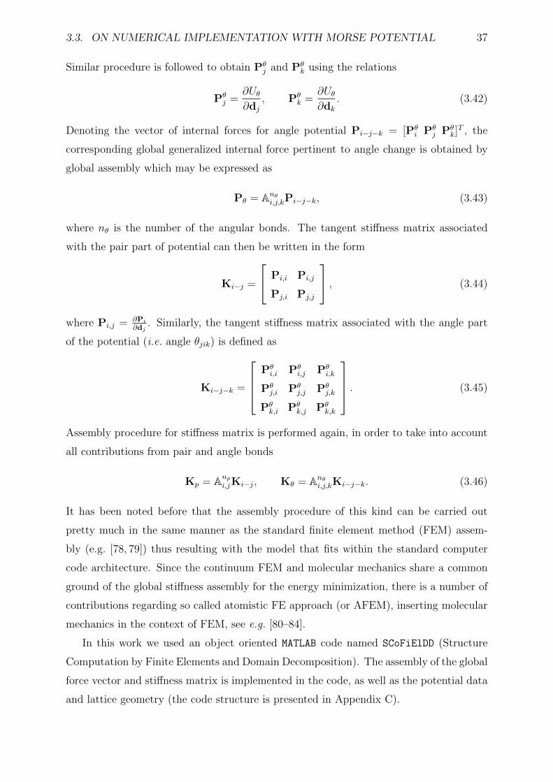
3.3. ON NUMERICAL IMPLEMENTATION WITH MORSE POTENTIAL 37
Similar procedure is followed to obtain Pθj and Pθ
k using the relations
Pθj =
∂Uθ∂dj
, Pθk =
∂Uθ∂dk
. (3.42)
Denoting the vector of internal forces for angle potential Pi−j−k = [Pθi Pθ
j Pθk]T , the
corresponding global generalized internal force pertinent to angle change is obtained by
global assembly which may be expressed as
Pθ = Anθi,j,kPi−j−k, (3.43)
where nθ is the number of the angular bonds. The tangent stiffness matrix associated
with the pair part of potential can then be written in the form
Ki−j =
Pi,i Pi,j
Pj,i Pj,j
, (3.44)
where Pi,j = ∂Pi∂dj
. Similarly, the tangent stiffness matrix associated with the angle part
of the potential (i.e. angle θjik) is defined as
Ki−j−k =
Pθi,i Pθ
i,j Pθi,k
Pθj,i Pθ
j,j Pθj,k
Pθk,i Pθ
k,j Pθk,k
. (3.45)
Assembly procedure for stiffness matrix is performed again, in order to take into account
all contributions from pair and angle bonds
Kp = Anpi,jKi−j, Kθ = Anθ
i,j,kKi−j−k. (3.46)
It has been noted before that the assembly procedure of this kind can be carried out
pretty much in the same manner as the standard finite element method (FEM) assem-
bly (e.g. [78, 79]) thus resulting with the model that fits within the standard computer
code architecture. Since the continuum FEM and molecular mechanics share a common
ground of the global stiffness assembly for the energy minimization, there is a number of
contributions regarding so called atomistic FE approach (or AFEM), inserting molecular
mechanics in the context of FEM, see e.g. [80–84].
In this work we used an object oriented MATLAB code named SCoFiElDD (Structure
Computation by Finite Elements and Domain Decomposition). The assembly of the global
force vector and stiffness matrix is implemented in the code, as well as the potential data
and lattice geometry (the code structure is presented in Appendix C).

38 CHAPTER 3. ATOMISTIC MODELING
Chapter 4Equivalent continuum modelling
In this chapter we introduce the approach of building an equivalent continuum model
that should be capable to substitute the atomistic model of nano-structure given in the
previous chapter. This approach resembles the hierarchical type of MS methods, as
briefly discussed in the introduction. However, since many interesting processes cannot
be described nor completely understood by surrogate continuum model, the approach
introduced herein is reserved exclusively for the effective modelling of pristine (defect free)
nano-structures. Furthermore, continuum model together with the coupling strategy is
extensively used for the concurrent atomistic-to-continuum MS material modelling, that
will be discussed in the following chapter. Thus, the developments presented in this
chapter pertain to the common way to construct the continuum model used mostly in the
BD based coupling.
The surrogate model should be selected as the most “compatible” one with the atom-
istic, in the sense of homogenization. The choice of this model depends on both the nature
of the material and loading conditions. The former is determined by the lattice geometry
and interatomic potential (Chapter 3), while the latter is simply related to the small or
large strain regime and corresponding linear or geometrically nonlinear framework (here).
Thus, the material parameters of the surrogate continuum constitutive model should be
calibrated accordingly. To that end, there are two approaches that appear in the litera-
ture related to atomistic-to-continuum coupling, see [85]. The first one is related to the
construction of constitutive equation via the Cauchy-Born rule (see e.g. [86, 87]) intro-
duced in the quasi-continuum (QC) approach (e.g. in [33, 88]). The Cauchy-Born rule
is described in detail in Chapter 5 (Sec. 5.2.2). We focus here on the second approach
which pertains to computing the equivalent continuum model parameters through numer-
ical homogenization. The latter considers calibrating the continuum model parameters
by means of the virtual experiments on the representative volume element (RVE). In the
39
40 CHAPTER 4. EQUIVALENT CONTINUUM MODELLING
developments to follow, we present parameters calibration for the graphene lattice driven
by the Morse potential in small and large strain regime.
4.1 Virtual experiments on atomistic lattice
The illustration of the calibration procedure to obtain the elastic modulus (i.e. the linear
elastic continuum) by simply considering a representative cell of springs which represents
bonds in the chain-like, one-dimensional (1D) case is given in [36]. More systematic
approach that exploits the virtual experiments on the RVE is suggested in [39], where
the virtual experiments are performed on series of RVE’s. The RVE is considered to be
a piece of pristine, generic, rectangular, atomistic lattice whose dimension is iteratively
increased until the consistent homogenized elastic continuum is obtained. The choice of
the continuum model is, naturally, problem dependent, see [38] for nonlinear hyperelastic
material model suitable for polymeric materials. The criteria for the homogenized medium
is fulfilled when the energy and/or the material parameters do not vary significantly with
further size increase. In this iterative process, the energy tends to converge to the one of
the infinite lattice, often referred to as ’bulk’.
We introduce this approach for graphene lattice by means of simple uniaxial tests
on the nearly square RVE’s. The geometry, boundary conditions and computational
procedure concerning virtual experiments is given in sequel (see Figure 4.1). At first we
will discuss the small strain regime and model it as a plane stress linear elastic continuum
(Section 4.2). Furthermore, we also show the behaviour of the SLGS samples in nonlinear
regime showing the change of the tangential Young’s modulus with advancing strain.
Averaged continuum properties of graphene in the context of infinitesimal deformation
is the subject of research for nearly 10 past years. However there is a large discrepancy
in the results obtained by means of the different simulation methods and experimental
study (see our paper [77]).
Equivalent continuum modeling of large deformations of graphene goes beyond what linear
theory can handle. Thus, in the second part of this chapter we seek to adapt the nonlinear
membrane theory which includes, as a special case, the hyperelastic model in terms of
principal stretches. The latter was often used to characterise rubberlike materials, see [89].
In order to obtain a constitutive law in terms of principal stretches for large deformation
of graphene, we will perform a series of biaxial virtual experiments on the graphene lattice
samples. We measure the strain energy density and perform best fit to have the closed
form surrogate continuum model.
4.2. MATCHING AT. AND CONT. MODELS, SMALL STRAIN 41
4.2 Matching the atomistic and continuum models in
small strain regime
In small strain regime we tend to use (as the surrogate model) the continuum model
based on isotropic, linear elasticity defined by the two parameters, namely Young’s mod-
ulus, E, and Poisson ratio, ν. The vast majority of previously proposed formulations
and computational methods leads to radically different results regarding graphene’s elas-
tic properties. We present in this section a review of some recent research, and more
importantly, we identify the main mechanisms resulting in such a large dispersion of elas-
tic properties. Furthermore, we clarify the influence on computed results by the main
model ingredients, such as specimen size, chirality of microstructure, the effect of chosen
boundary conditions (imposed displacement versus force), and the corresponding plane
stress transformation. The proposed approach is capable of explaining the scatter of the
results for computed stresses, energy and stiffness, and provide the bounds on graphene
elastic properties, which are quite important in modeling and simulation of the virtual
experiments on graphene based devices.
4.2.1 Linear elastic properties of graphene
Literature review
A review of the large scatter of Young’s modulus value was mentioned for the first time
in [90]. The same work also gave a MM study of two initial configurations, with and with-
out equilibrium adjustment of atoms before loading process. The main conclusion was
that the computed values fit in two groups. First, the values of E around 700 GPa and
then those of around 1000 GPa. These correspond to the minimized (equilibrium) and un-
minimized (with no potential minimisation) configuration, respectively. The interatomic
potential used therein is the Tersoff-Brenner, defined as pair potential with the addition
of cut-off function and multibody parameter (as described in Section 3.2). This poten-
tial when minimized (i.e. solved for the unloaded configuration) yields slightly different
configuration than initial formed of regular hexagonal structure. This effect is due to co-
ordination number i.e. the different number of neighbouring atoms on the boundary, and
is noticeable near the boundary of the lattice driven with TB potential. The bond length
of interior bonds in the finite graphene is already close to that of bulk graphene. They
conclude that the minimisation of potential is one of the reasons for Young’s modulus
scatter. The prescribed displacement is used on the edges of rather small graphene sam-
42 CHAPTER 4. EQUIVALENT CONTINUUM MODELLING
ple consisting of 120 atoms (around 1.5nm × 1.5nm). The results are in good agreement
with the ones presented in [91]. In [90] they also consider two models in the analysis,
with only two or all four edges constrained to be straight. Up to our knowledge this
is the only research that includes the influence of boundary conditions on the elastic
properties of graphene, even though it is by no means systematic. In [92] tight-binding
(reported E = 910 GPa) and MD methods (reported E = 1010± 30 GPa) with reactive
bond-order (REBO) potential are used to study mechanical properties of graphene i.e.
stripes of graphene called GNR. They perform uniaxial tensile tests using MD under: 1)
deformation-control with periodic boundary conditions to study the chirality effects on
bulk (infinite size) graphene, or 2) force-control to study size and chirality effects of GNR
(finite). They show the convergence of E with the size of the GNR and the influence of the
chirality (armchair versus zigzag) on computed value of Young’s modulus. The results are
in reasonable agreement with experiments which report E = 1000±100 GPa (see [9]) and
ab initio simulation (see [93] or [94]). Similar tension analysis using MD is done by Xu [95]
with emphasis on the dynamical effects on fracture. Lu et al. [96] and [97] pointed out the
effect of edge structures on the mechanical behavior of GNR’s. Particularly, they focus
on nonlinear behavior of GNR’s under quasi-static uniaxial tension using MM, emphasiz-
ing the effects of armchair and zigzag edges (without and with hydrogen passivation) on
elastic modulus and fracture. They report Youngs modulus to be 714 GPa using REBO
potential. Another interesting strategy to model nanostructures, introduced in [98], is
based on the so-called equivalent atomistic continuum-structural mechanics approach. In
this approach, typical finite elements of structural mechanics, such as bar, beam and shell,
are used with appropriate mechanical properties to simulate the behaviour of graphene
layers and carbon nanotubes. An extension of the truss-lattice (FEM) model from [98] is
proposed in [99] where the equivalent atomistic continuum-structural mechanics approach
is combined with the theory of cellular solids micromechanics. The AMBER and Morse
interatomic potentials are used, and closed form solutions for the in-plane elastic proper-
ties of SLGS are given. In [100] a structural mechanics approach was used based upon
nonlinear spring finite element (FE) to simulate the SLGS behaviour represented by mod-
ified Morse potential. The latter approach is used in [101] to show how size and chirality
influence mechanical properties of SLGS. Besides mentioned study, an exhaustive litera-
ture review of the mechanical properties of SLGS is presented in [101], separating them
in three groups. The first group is related to the use of MD method for which Young’s
modulus remains in the range E = 710 . . . 1200 GPa. The MM i.e. structural mechan-
ics methods form the second group and ranges from 940 to 5510 GPa. Finally, for the
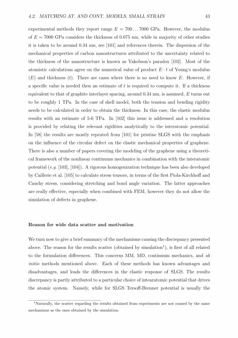
4.2. MATCHING AT. AND CONT. MODELS, SMALL STRAIN 43
experimental methods they report range E = 700 . . . 7000 GPa. However, the modulus
of E = 7000 GPa considers the thickness of 0.075 nm, while in majority of other studies
it is taken to be around 0.34 nm, see [101] and references therein. The dispersion of the
mechanical properties of carbon nanostructures attributed to the uncertainty related to
the thickness of the nanostructure is known as Yakobson’s paradox [102]. Most of the
atomistic calculations agree on the numerical value of product E · t of Young’s modulus
(E) and thickness (t). There are cases where there is no need to know E. However, if
a specific value is needed then an estimate of t is required to compute it. If a thickness
equivalent to that of graphite interlayer spacing, around 0.34 nm, is assumed, E turns out
to be roughly 1 TPa. In the case of shell model, both the tension and bending rigidity
needs to be calculated in order to obtain the thickness. In this case, the elastic modulus
results with an estimate of 5-6 TPa. In [102] this issue is addressed and a resolution
is provided by relating the relevant rigidities analytically to the interatomic potential.
In [58] the results are mostly repeated from [101] for pristine SLGS with the emphasis
on the influence of the circular defect on the elastic mechanical properties of graphene.
There is also a number of papers covering the modeling of the graphene using a theoreti-
cal framework of the nonlinear continuum mechanics in combination with the interatomic
potential (e.g. [103], [104]). A rigorous homogenization technique has been also developed
by Caillerie et al. [105] to calculate stress tensors, in terms of the first Piola-Kirchhoff and
Cauchy stress, considering stretching and bond angle variation. The latter approaches
are really effective, especially when combined with FEM, however they do not allow the
simulation of defects in graphene.
Reason for wide data scatter and motivation
We turn now to give a brief summary of the mechanisms causing the discrepancy presented
above. The reason for the results scatter (obtained by simulation1), is first of all related
to the formulation differences. This concerns MM, MD, continuum mechanics, and ab
initio methods mentioned above. Each of these methods has known advantages and
disadvantages, and leads the differences in the elastic response of SLGS. The results
discrepancy is partly attributed to a particular choice of intearatomic potential that drives
the atomic system. Namely, while for SLGS Tersoff-Brenner potential is usually the
1Naturally, the scatter regarding the results obtained from experiments are not caused by the same
mechanisms as the ones obtained by the simulation.
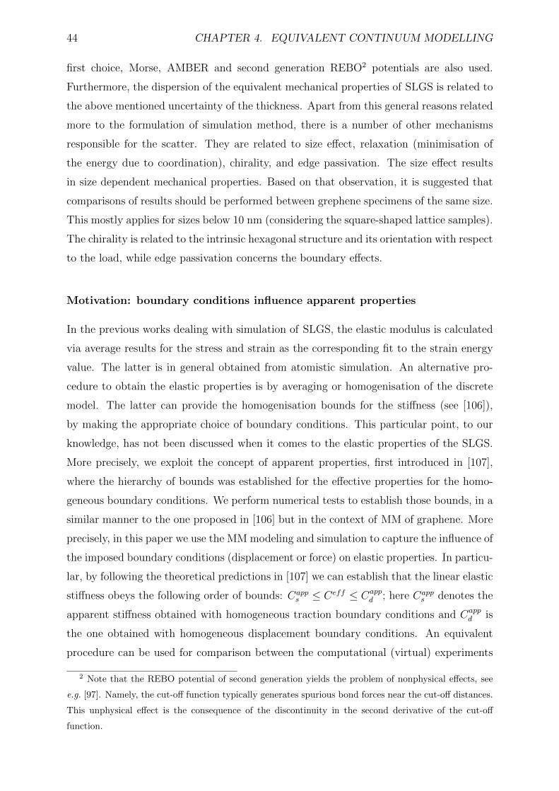
44 CHAPTER 4. EQUIVALENT CONTINUUM MODELLING
first choice, Morse, AMBER and second generation REBO2 potentials are also used.
Furthermore, the dispersion of the equivalent mechanical properties of SLGS is related to
the above mentioned uncertainty of the thickness. Apart from this general reasons related
more to the formulation of simulation method, there is a number of other mechanisms
responsible for the scatter. They are related to size effect, relaxation (minimisation of
the energy due to coordination), chirality, and edge passivation. The size effect results
in size dependent mechanical properties. Based on that observation, it is suggested that
comparisons of results should be performed between grephene specimens of the same size.
This mostly applies for sizes below 10 nm (considering the square-shaped lattice samples).
The chirality is related to the intrinsic hexagonal structure and its orientation with respect
to the load, while edge passivation concerns the boundary effects.
Motivation: boundary conditions influence apparent properties
In the previous works dealing with simulation of SLGS, the elastic modulus is calculated
via average results for the stress and strain as the corresponding fit to the strain energy
value. The latter is in general obtained from atomistic simulation. An alternative pro-
cedure to obtain the elastic properties is by averaging or homogenisation of the discrete
model. The latter can provide the homogenisation bounds for the stiffness (see [106]),
by making the appropriate choice of boundary conditions. This particular point, to our
knowledge, has not been discussed when it comes to the elastic properties of the SLGS.
More precisely, we exploit the concept of apparent properties, first introduced in [107],
where the hierarchy of bounds was established for the effective properties for the homo-
geneous boundary conditions. We perform numerical tests to establish those bounds, in a
similar manner to the one proposed in [106] but in the context of MM of graphene. More
precisely, in this paper we use the MM modeling and simulation to capture the influence of
the imposed boundary conditions (displacement or force) on elastic properties. In particu-
lar, by following the theoretical predictions in [107] we can establish that the linear elastic
stiffness obeys the following order of bounds: Capps ≤ Ceff ≤ Capp
d ; here Capps denotes the
apparent stiffness obtained with homogeneous traction boundary conditions and Cappd is
the one obtained with homogeneous displacement boundary conditions. An equivalent
procedure can be used for comparison between the computational (virtual) experiments
2 Note that the REBO potential of second generation yields the problem of nonphysical effects, see
e.g. [97]. Namely, the cut-off function typically generates spurious bond forces near the cut-off distances.
This unphysical effect is the consequence of the discontinuity in the second derivative of the cut-off
function.
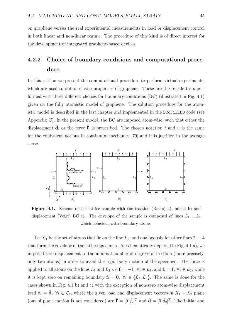
4.2. MATCHING AT. AND CONT. MODELS, SMALL STRAIN 45
on graphene versus the real experimental measurements in load or displacement control
in both linear and non-linear regime. The procedure of this kind is of direct interest for
the development of integrated graphene-based devices.
4.2.2 Choice of boundary conditions and computational proce-
dure
In this section we present the computational procedure to perform virtual experiments,
which are used to obtain elastic properties of graphene. These are the tensile tests per-
formed with three different choices for boundary conditions (BC) (illustrated in Fig. 4.1)
given on the fully atomistic model of graphene. The solution procedure for the atom-
istic model is described in the last chapter and implemented in the SCoFiElDD code (see
Appendix C). In the present model, the BC are imposed atom-wise, such that either the
displacement di or the force fi is prescribed. The chosen notation t and u is the same
for the equivalent notions in continuum mechanics [79] and it is justified in the average
sense.
a) b) c)
Armchair (A)
Zigzag (Z)
c)
Figure 4.1. Scheme of the lattice sample with the traction (Reuss) a), mixed b) and
displacement (Voigt) BC c). The envelope of the sample is composed of lines L1 . . . L4
which coincides with boundary atoms.
Let L1 be the set of atoms that lie on the line L1, and analogously for other lines 2 . . . 4
that form the envelope of the lattice specimen. As schematically depicted in Fig. 4.1 a), we
imposed zero displacement to the minimal number of degrees of freedom (more precisely,
only two atoms) in order to avoid the rigid body motion of the specimen. The force is
applied to all atoms on the lines L1 and L2 i.e. fi = −f , ∀i ∈ L1, and fi = f , ∀i ∈ L2, while
it is kept zero on remaining boundary fi = 0, ∀i ∈ L3,L4. The same is done for the
cases shown in Fig. 4.1 b) and c) with the exception of non-zero atom-wise displacement
load di = d, ∀i ∈ L2, where the given load and displacement vectors in X1 − X2 plane
(out of plane motion is not considered) are f = [0 f2]T and d = [0 d2]T . The initial and
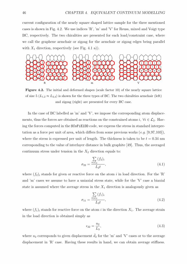
46 CHAPTER 4. EQUIVALENT CONTINUUM MODELLING
current configuration of the nearly square shaped lattice sample for the three mentioned
cases is shown in Fig. 4.2. We use indices ’R’, ’m’ and ’V’ for Reuss, mixed and Voigt type
BC, respectively. The two chiralities are presented for each load/constraint case, where
we call the graphene armchair or zigzag for the armchair or zigzag edges being parallel
with X1 direction, respectively (see Fig. 4.1 a)).
R m V
Figure 4.2. The initial and deformed shapes (scale factor 10) of the nearly square lattice
of size 5 (L1,2 ≈ L3,4) is shown for the three types of BC. The two chiralities armchair (left)
and zigzag (right) are presented for every BC case.
In the case of BC labelled as ’m’ and ’V’, we impose the corresponding atom displace-
ments, thus the forces are obtained as reactions on the constrained atoms i, ∀i ∈ L2. Hav-
ing the forces computed in the SCoFiElDD code, we express the stress in standard interpre-
tation as a force per unit of area, which differs from some previous works (e.g. [9,97,103]),
where the stress is expressed per unit of length. The thickness is taken to be t = 0.34 nm
corresponding to the value of interlayer distance in bulk graphite [49]. Thus, the averaged
continuum stress under tension in the X2 direction equals to:
σ22 =
∑i∈L2
(f2)i
L2t, (4.1)
where (f2)i stands for given or reactive force on the atom i in load direction. For the ’R’
and ’m’ cases we assume to have a uniaxial stress state, while for the ’V’ case a biaxial
state is assumed where the average stress in the X1 direction is analogously given as
σ11 =
∑i∈L3
(f1)i
L3t, (4.2)
where (f1)i stands for reactive force on the atom i in the direction X1. The average strain
in the load direction is obtained simply as
ε22 =u2
L3
, (4.3)
where u2 corresponds to given displacement d2 for the ’m’ and ’V’ cases or to the average
displacement in ’R’ case. Having these results in hand, we can obtain average stiffness.
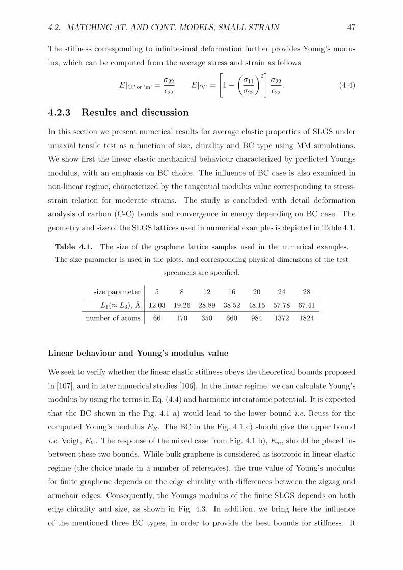
4.2. MATCHING AT. AND CONT. MODELS, SMALL STRAIN 47
The stiffness corresponding to infinitesimal deformation further provides Young’s modu-
lus, which can be computed from the average stress and strain as follows
E|’R’ or ’m’ =σ22
ε22
E|’V’ =
[1−
(σ11
σ22
)2]σ22
ε22
. (4.4)
4.2.3 Results and discussion
In this section we present numerical results for average elastic properties of SLGS under
uniaxial tensile test as a function of size, chirality and BC type using MM simulations.
We show first the linear elastic mechanical behaviour characterized by predicted Youngs
modulus, with an emphasis on BC choice. The influence of BC case is also examined in
non-linear regime, characterized by the tangential modulus value corresponding to stress-
strain relation for moderate strains. The study is concluded with detail deformation
analysis of carbon (C-C) bonds and convergence in energy depending on BC case. The
geometry and size of the SLGS lattices used in numerical examples is depicted in Table 4.1.
Table 4.1. The size of the graphene lattice samples used in the numerical examples.
The size parameter is used in the plots, and corresponding physical dimensions of the test
specimens are specified.
size parameter 5 8 12 16 20 24 28
L1(≈ L3), A 12.03 19.26 28.89 38.52 48.15 57.78 67.41
number of atoms 66 170 350 660 984 1372 1824
Linear behaviour and Young’s modulus value
We seek to verify whether the linear elastic stiffness obeys the theoretical bounds proposed
in [107], and in later numerical studies [106]. In the linear regime, we can calculate Young’s
modulus by using the terms in Eq. (4.4) and harmonic interatomic potential. It is expected
that the BC shown in the Fig. 4.1 a) would lead to the lower bound i.e. Reuss for the
computed Young’s modulus ER. The BC in the Fig. 4.1 c) should give the upper bound
i.e. Voigt, EV . The response of the mixed case from Fig. 4.1 b), Em, should be placed in-
between these two bounds. While bulk graphene is considered as isotropic in linear elastic
regime (the choice made in a number of references), the true value of Young’s modulus
for finite graphene depends on the edge chirality with differences between the zigzag and
armchair edges. Consequently, the Youngs modulus of the finite SLGS depends on both
edge chirality and size, as shown in Fig. 4.3. In addition, we bring here the influence
of the mentioned three BC types, in order to provide the best bounds for stiffness. It
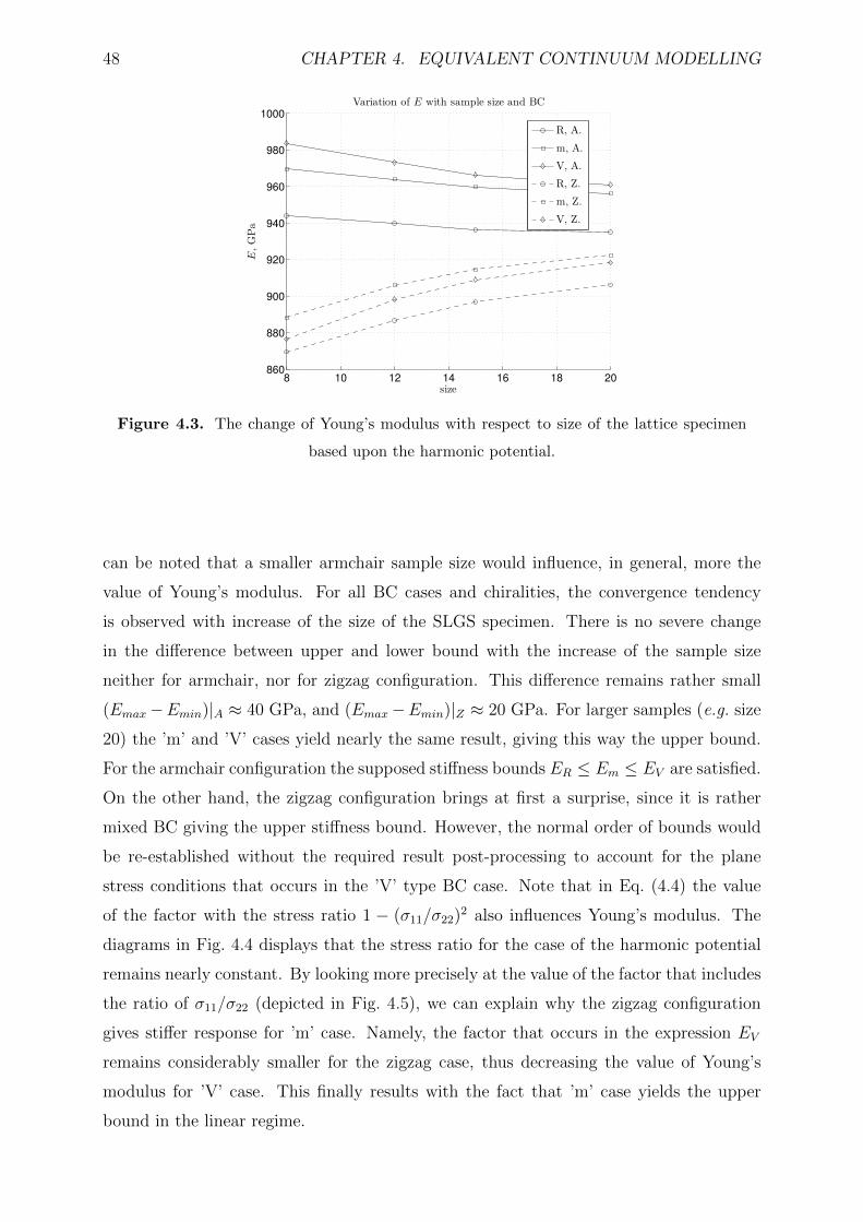
48 CHAPTER 4. EQUIVALENT CONTINUUM MODELLING
8 10 12 14 16 18 20860
880
900
920
940
960
980
1000
Variation of E with sample size and BC
size
E,GPa
R, A.
m, A.
V, A.
R, Z.
m, Z.
V, Z.
Figure 4.3. The change of Young’s modulus with respect to size of the lattice specimen
based upon the harmonic potential.
can be noted that a smaller armchair sample size would influence, in general, more the
value of Young’s modulus. For all BC cases and chiralities, the convergence tendency
is observed with increase of the size of the SLGS specimen. There is no severe change
in the difference between upper and lower bound with the increase of the sample size
neither for armchair, nor for zigzag configuration. This difference remains rather small
(Emax−Emin)|A ≈ 40 GPa, and (Emax−Emin)|Z ≈ 20 GPa. For larger samples (e.g. size
20) the ’m’ and ’V’ cases yield nearly the same result, giving this way the upper bound.
For the armchair configuration the supposed stiffness bounds ER ≤ Em ≤ EV are satisfied.
On the other hand, the zigzag configuration brings at first a surprise, since it is rather
mixed BC giving the upper stiffness bound. However, the normal order of bounds would
be re-established without the required result post-processing to account for the plane
stress conditions that occurs in the ’V’ type BC case. Note that in Eq. (4.4) the value
of the factor with the stress ratio 1 − (σ11/σ22)2 also influences Young’s modulus. The
diagrams in Fig. 4.4 displays that the stress ratio for the case of the harmonic potential
remains nearly constant. By looking more precisely at the value of the factor that includes
the ratio of σ11/σ22 (depicted in Fig. 4.5), we can explain why the zigzag configuration
gives stiffer response for ’m’ case. Namely, the factor that occurs in the expression EV
remains considerably smaller for the zigzag case, thus decreasing the value of Young’s
modulus for ’V’ case. This finally results with the fact that ’m’ case yields the upper
bound in the linear regime.
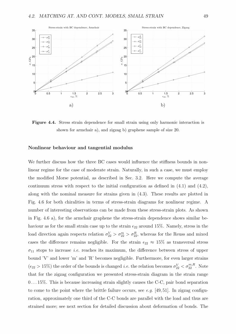
4.2. MATCHING AT. AND CONT. MODELS, SMALL STRAIN 49
0 0.5 1 1.5 2 2.5 30
5
10
15
20
25
30
35
Stress-strain with BC dependence, Armchair
ǫ22, %
σ,GPa
σR
22
σm
22
σV
22
σV
11
a)
0 0.5 1 1.5 2 2.5 30
5
10
15
20
25
30
35
Stress-strain with BC dependence, Zigzag
ǫ22, %
σ,GPa
σR
22
σm
22
σV
22
σV
11
b)
Figure 4.4. Stress strain dependence for small strain using only harmonic interaction is
shown for armchair a), and zigzag b) graphene sample of size 20.
Nonlinear behaviour and tangential modulus
We further discuss how the three BC cases would influence the stiffness bounds in non-
linear regime for the case of moderate strain. Naturally, in such a case, we must employ
the modified Morse potential, as described in Sec. 3.2. Here we compute the average
continuum stress with respect to the initial configuration as defined in (4.1) and (4.2),
along with the nominal measure for strains given in (4.3). These results are plotted in
Fig. 4.6 for both chiralities in terms of stress-strain diagrams for nonlinear regime. A
number of interesting observations can be made from these stress-strain plots. As shown
in Fig. 4.6 a), for the armchair graphene the stress-strain dependence shows similar be-
haviour as for the small strain case up to the strain ε22 around 15%. Namely, stress in the
load direction again respects relation σV22 > σm22 > σR22, whereas for the Reuss and mixed
cases the difference remains negligible. For the strain ε22 ≈ 15% as transversal stress
σ11 stops to increase i.e. reaches its maximum, the difference between stress of upper
bound ’V’ and lower ’m’ and ’R’ becomes negligible. Furthermore, for even larger strains
(ε22 > 15%) the order of the bounds is changed i.e. the relation becomes σV22 < σm,R22 . Note
that for the zigzag configuration we presented stress-strain diagram in the strain range
0 . . . 15%. This is because increasing strain slightly causes the C-C, pair bond separation
to come to the point where the brittle failure occurs, see e.g. [49, 51]. In zigzag configu-
ration, approximately one third of the C-C bonds are parallel with the load and thus are
strained more; see next section for detailed discussion about deformation of bonds. The
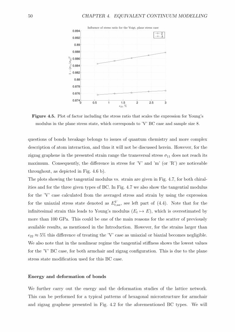
50 CHAPTER 4. EQUIVALENT CONTINUUM MODELLING
0 0.5 1 1.5 2 2.5 30.874
0.876
0.878
0.88
0.882
0.884
0.886
0.888
0.89
0.892
0.894
Influence of stress ratio for the Voigt, plane stress case
ǫ22, %
1−
(σ11/σ22)2
ZA
Figure 4.5. Plot of factor including the stress ratio that scales the expression for Young’s
modulus in the plane stress state, which corresponds to ’V’ BC case and sample size 8.
questions of bonds breakage belongs to issues of quantum chemistry and more complex
description of atom interaction, and thus it will not be discussed herein. However, for the
zigzag graphene in the presented strain range the transversal stress σ11 does not reach its
maximum. Consequently, the difference in stress for ’V’ and ’m’ (or ’R’) are noticeable
throughout, as depicted in Fig. 4.6 b).
The plots showing the tangential modulus vs. strain are given in Fig. 4.7, for both chiral-
ities and for the three given types of BC. In Fig. 4.7 we also show the tangential modulus
for the ’V’ case calculated from the averaged stress and strain by using the expression
for the uniaxial stress state denoted as EVt,ua, see left part of (4.4). Note that for the
infinitesimal strain this leads to Young’s modulus (Et 7→ E), which is overestimated by
more than 100 GPa. This could be one of the main reasons for the scatter of previously
available results, as mentioned in the Introduction. However, for the strains larger than
ε22 ≈ 5% this difference of treating the ’V’ case as uniaxial or biaxial becomes negligible.
We also note that in the nonlinear regime the tangential stiffness shows the lowest values
for the ’V’ BC case, for both armchair and zigzag configuration. This is due to the plane
stress state modification used for this BC case.
Energy and deformation of bonds
We further carry out the energy and the deformation studies of the lattice network.
This can be performed for a typical patterns of hexagonal microstructure for armchair
and zigzag graphene presented in Fig. 4.2 for the aforementioned BC types. We will
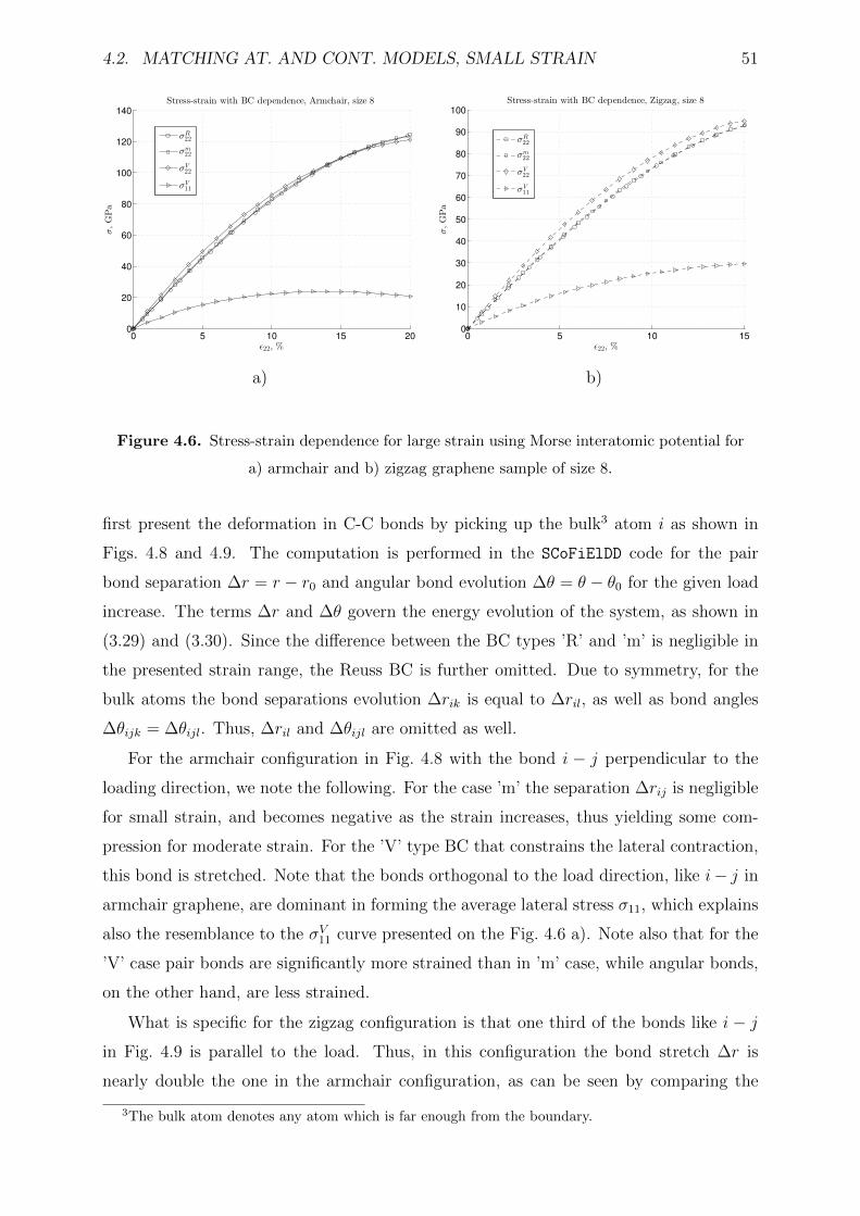
4.2. MATCHING AT. AND CONT. MODELS, SMALL STRAIN 51
0 5 10 15 200
20
40
60
80
100
120
140
Stress-strain with BC dependence, Armchair, size 8
ǫ22, %
σ,GPa
σR
22
σm
22
σV
22
σV
11
a)
0 5 10 150
10
20
30
40
50
60
70
80
90
100
Stress-strain with BC dependence, Zigzag, size 8
ǫ22, %
σ,GPa
σR
22
σm
22
σV
22
σV
11
b)
Figure 4.6. Stress-strain dependence for large strain using Morse interatomic potential for
a) armchair and b) zigzag graphene sample of size 8.
first present the deformation in C-C bonds by picking up the bulk3 atom i as shown in
Figs. 4.8 and 4.9. The computation is performed in the SCoFiElDD code for the pair
bond separation ∆r = r − r0 and angular bond evolution ∆θ = θ − θ0 for the given load
increase. The terms ∆r and ∆θ govern the energy evolution of the system, as shown in
(3.29) and (3.30). Since the difference between the BC types ’R’ and ’m’ is negligible in
the presented strain range, the Reuss BC is further omitted. Due to symmetry, for the
bulk atoms the bond separations evolution ∆rik is equal to ∆ril, as well as bond angles
∆θijk = ∆θijl. Thus, ∆ril and ∆θijl are omitted as well.
For the armchair configuration in Fig. 4.8 with the bond i − j perpendicular to the
loading direction, we note the following. For the case ’m’ the separation ∆rij is negligible
for small strain, and becomes negative as the strain increases, thus yielding some com-
pression for moderate strain. For the ’V’ type BC that constrains the lateral contraction,
this bond is stretched. Note that the bonds orthogonal to the load direction, like i− j in
armchair graphene, are dominant in forming the average lateral stress σ11, which explains
also the resemblance to the σV11 curve presented on the Fig. 4.6 a). Note also that for the
’V’ case pair bonds are significantly more strained than in ’m’ case, while angular bonds,
on the other hand, are less strained.
What is specific for the zigzag configuration is that one third of the bonds like i − jin Fig. 4.9 is parallel to the load. Thus, in this configuration the bond stretch ∆r is
nearly double the one in the armchair configuration, as can be seen by comparing the
3The bulk atom denotes any atom which is far enough from the boundary.
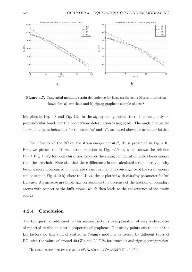
52 CHAPTER 4. EQUIVALENT CONTINUUM MODELLING
0 5 10 15 200
200
400
600
800
1000
1200
Tangential modulus vs. strain, Armchair, size 8
ǫ22, %
Et,GPa
ERt
Emt
EVt
EVt,ua
a)
0 5 10 150
200
400
600
800
1000
1200
Tangential modulus vs. strain, Zigzag, size 8
ǫ22, %
Et,GPa
ERt
Emt
EVt
EVt,ua
b)
Figure 4.7. Tangential modulus-strain dependence for large strain using Morse interaction
shown for: a) armchair and b) zigzag graphene sample of size 8.
left plots in Fig. 4.8 and Fig. 4.9. In the zigzag configuration, there is consequently no
perpendicular bond, nor the bond whose deformation is negligible. The angle change ∆θ
shows analogous behaviour for the cases ’m’ and ’V’, as stated above for armchair lattice.
The influence of the BC on the strain energy density4, W , is presented in Fig. 4.10.
First we picture the W vs. strain relation in Fig. 4.10 a), which shows the relation
WR ≤ Wm ≤ WV for both chiralities, however the zigzag configuration yields lower energy
than the armchair. Note also that these differences in the calculated strain energy density
become more pronounced in moderate strain regime. The convergence of the strain energy
can be seen in Fig. 4.10 b) where the W vs. size is plotted with chirality parameter for ’m’
BC case. An increase in sample size corresponds to a decrease of the fraction of boundary
atoms with respect to the bulk atoms, which then leads to the convergence of the strain
energy.
4.2.4 Conclusion
The key question addressed in this section pertains to explanation of very wide scatter
of reported results on elastic properties of graphene. Our study points out to one of the
key factors for this kind of scatter in Young’s modulus as caused by different types of
BC, with the values of around 40 GPa and 20 GPa for armchair and zigzag configuration,
4The strain energy density is given in eV/A, where 1 eV=1.60217657 · 10−19 J.
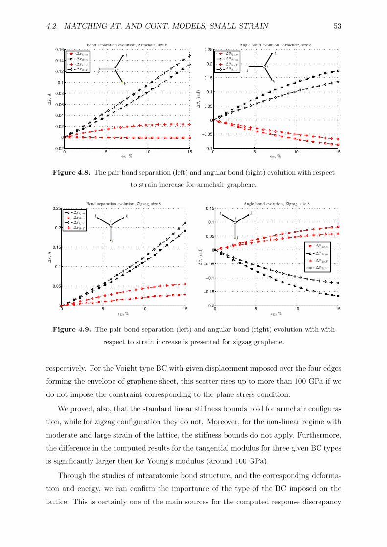
4.2. MATCHING AT. AND CONT. MODELS, SMALL STRAIN 53
Figure 4.8. The pair bond separation (left) and angular bond (right) evolution with respect
to strain increase for armchair graphene.
Figure 4.9. The pair bond separation (left) and angular bond (right) evolution with with
respect to strain increase is presented for zigzag graphene.
respectively. For the Voight type BC with given displacement imposed over the four edges
forming the envelope of graphene sheet, this scatter rises up to more than 100 GPa if we
do not impose the constraint corresponding to the plane stress condition.
We proved, also, that the standard linear stiffness bounds hold for armchair configura-
tion, while for zigzag configuration they do not. Moreover, for the non-linear regime with
moderate and large strain of the lattice, the stiffness bounds do not apply. Furthermore,
the difference in the computed results for the tangential modulus for three given BC types
is significantly larger then for Young’s modulus (around 100 GPa).
Through the studies of intearatomic bond structure, and the corresponding deforma-
tion and energy, we can confirm the importance of the type of the BC imposed on the
lattice. This is certainly one of the main sources for the computed response discrepancy
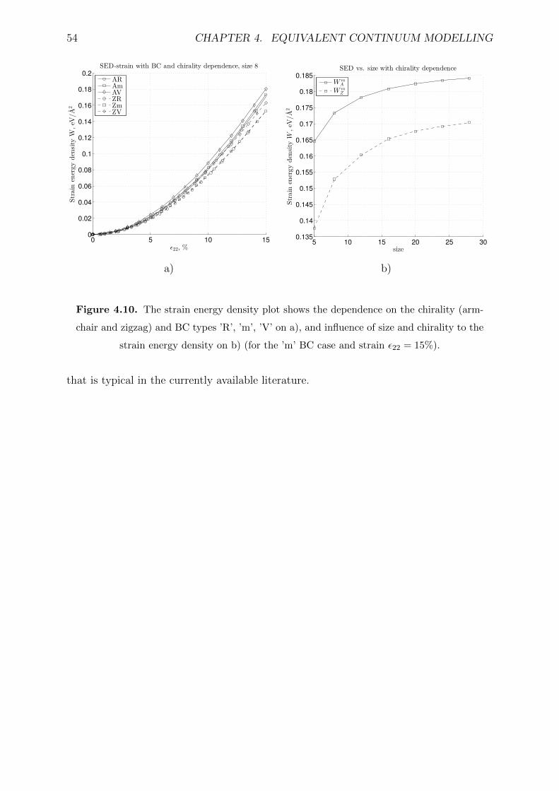
54 CHAPTER 4. EQUIVALENT CONTINUUM MODELLING
0 5 10 150
0.02
0.04
0.06
0.08
0.1
0.12
0.14
0.16
0.18
0.2
SED-strain with BC and chirality dependence, size 8
ǫ22, %
Strain
energydensity
W,eV
/A
2
ARAmAVZRZmZV
a)
5 10 15 20 25 300.135
0.14
0.145
0.15
0.155
0.16
0.165
0.17
0.175
0.18
0.185
SED vs. size with chirality dependence
size
Strain
energydensity
W,eV
/A
2
WmA
WmZ
b)
Figure 4.10. The strain energy density plot shows the dependence on the chirality (arm-
chair and zigzag) and BC types ’R’, ’m’, ’V’ on a), and influence of size and chirality to the
strain energy density on b) (for the ’m’ BC case and strain ε22 = 15%).
that is typical in the currently available literature.
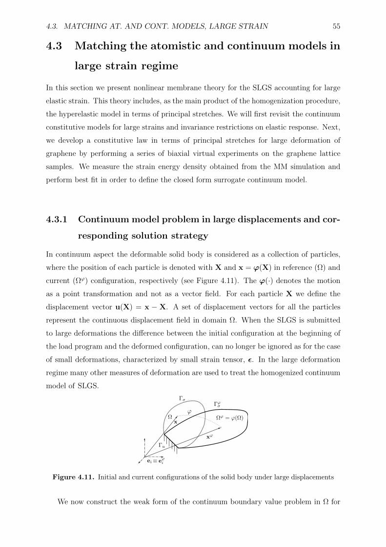
4.3. MATCHING AT. AND CONT. MODELS, LARGE STRAIN 55
4.3 Matching the atomistic and continuum models in
large strain regime
In this section we present nonlinear membrane theory for the SLGS accounting for large
elastic strain. This theory includes, as the main product of the homogenization procedure,
the hyperelastic model in terms of principal stretches. We will first revisit the continuum
constitutive models for large strains and invariance restrictions on elastic response. Next,
we develop a constitutive law in terms of principal stretches for large deformation of
graphene by performing a series of biaxial virtual experiments on the graphene lattice
samples. We measure the strain energy density obtained from the MM simulation and
perform best fit in order to define the closed form surrogate continuum model.
4.3.1 Continuum model problem in large displacements and cor-
responding solution strategy
In continuum aspect the deformable solid body is considered as a collection of particles,
where the position of each particle is denoted with X and x = ϕ(X) in reference (Ω) and
current (Ωϕ) configuration, respectively (see Figure 4.11). The ϕ(·) denotes the motion
as a point transformation and not as a vector field. For each particle X we define the
displacement vector u(X) = x − X. A set of displacement vectors for all the particles
represent the continuous displacement field in domain Ω. When the SLGS is submitted
to large deformations the difference between the initial configuration at the beginning of
the load program and the deformed configuration, can no longer be ignored as for the case
of small deformations, characterized by small strain tensor, ε. In the large deformation
regime many other measures of deformation are used to treat the homogenized continuum
model of SLGS.
Figure 4.11. Initial and current configurations of the solid body under large displacements
We now construct the weak form of the continuum boundary value problem in Ω for
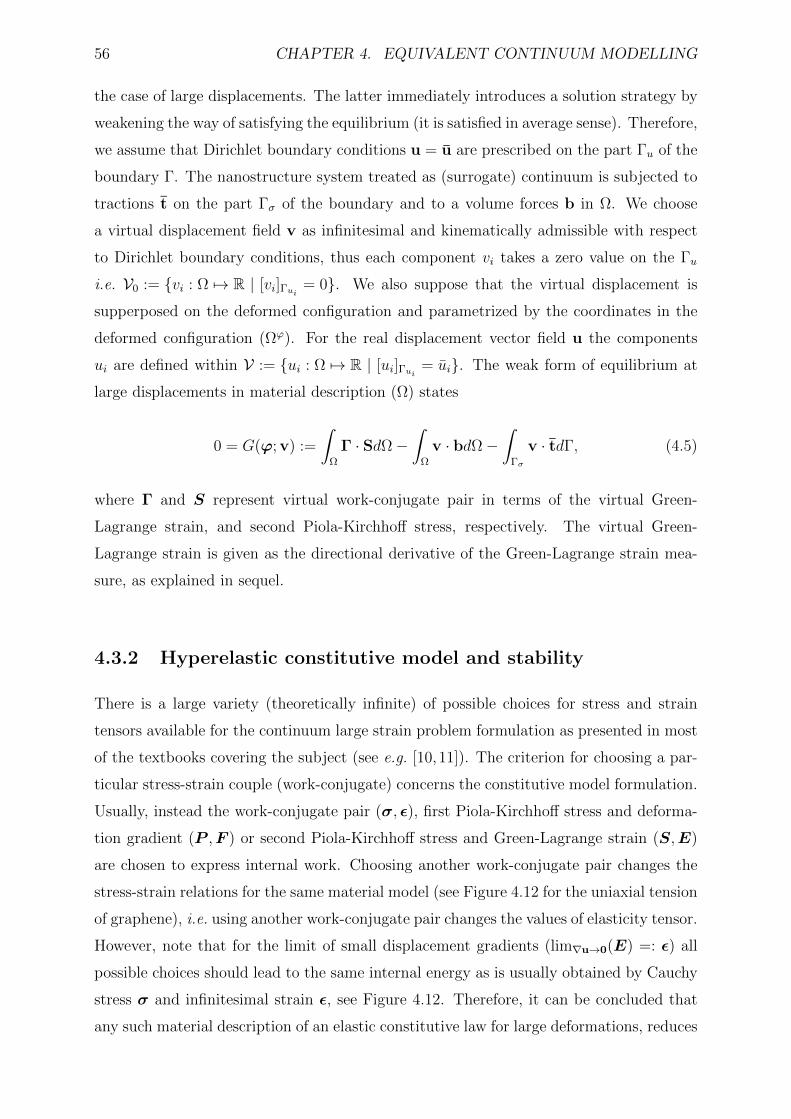
56 CHAPTER 4. EQUIVALENT CONTINUUM MODELLING
the case of large displacements. The latter immediately introduces a solution strategy by
weakening the way of satisfying the equilibrium (it is satisfied in average sense). Therefore,
we assume that Dirichlet boundary conditions u = u are prescribed on the part Γu of the
boundary Γ. The nanostructure system treated as (surrogate) continuum is subjected to
tractions t on the part Γσ of the boundary and to a volume forces b in Ω. We choose
a virtual displacement field v as infinitesimal and kinematically admissible with respect
to Dirichlet boundary conditions, thus each component vi takes a zero value on the Γu
i.e. V0 := vi : Ω 7→ R | [vi]Γui = 0. We also suppose that the virtual displacement is
supperposed on the deformed configuration and parametrized by the coordinates in the
deformed configuration (Ωϕ). For the real displacement vector field u the components
ui are defined within V := ui : Ω 7→ R | [ui]Γui = ui. The weak form of equilibrium at
large displacements in material description (Ω) states
0 = G(ϕ; v) :=
∫Ω
Γ · SdΩ−∫
Ω
v · bdΩ−∫
Γσ
v · tdΓ, (4.5)
where Γ and S represent virtual work-conjugate pair in terms of the virtual Green-
Lagrange strain, and second Piola-Kirchhoff stress, respectively. The virtual Green-
Lagrange strain is given as the directional derivative of the Green-Lagrange strain mea-
sure, as explained in sequel.
4.3.2 Hyperelastic constitutive model and stability
There is a large variety (theoretically infinite) of possible choices for stress and strain
tensors available for the continuum large strain problem formulation as presented in most
of the textbooks covering the subject (see e.g. [10,11]). The criterion for choosing a par-
ticular stress-strain couple (work-conjugate) concerns the constitutive model formulation.
Usually, instead the work-conjugate pair (σ, ε), first Piola-Kirchhoff stress and deforma-
tion gradient (P ,F ) or second Piola-Kirchhoff stress and Green-Lagrange strain (S,E)
are chosen to express internal work. Choosing another work-conjugate pair changes the
stress-strain relations for the same material model (see Figure 4.12 for the uniaxial tension
of graphene), i.e. using another work-conjugate pair changes the values of elasticity tensor.
However, note that for the limit of small displacement gradients (lim∇u→0(E) =: ε) all
possible choices should lead to the same internal energy as is usually obtained by Cauchy
stress σ and infinitesimal strain ε, see Figure 4.12. Therefore, it can be concluded that
any such material description of an elastic constitutive law for large deformations, reduces
4.3. MATCHING AT. AND CONT. MODELS, LARGE STRAIN 57
to Hooke’s law for the case of small deformation5. For the uniaxial tension of graphene
depicted in Figure 4.12 in the linear range between 0 − 2.5% it does not matter which
stress-strain relationship is used. In the nonlinear range, on the other hand, it is important
to use appropriate stress-strain measure for analysis.
0 0.05 0.1 0.15 0.20
10
20
30
40
50
60
70
80
90
100
strain
stress,GPa
σ22 − ǫ22
S22 − E22
Figure 4.12. Stress, strain plot (in direction x2 of graphene sample) showing the difference
between the Cauchy (true) stress vs. small strain and second Piola-Kirchhoff stress vs.
Green-Lagrange strain.
However, the unique form of the constitutive relation can be written for the hypere-
lastic material model in terms of the strain energy potential, W (·), since all possibilities
of stress and strain measure are only different material representations of the same work.
As an example we give the simplest, Saint-Venant-Kirchhoff (SVK) model in terms of the
Green-Lagrange strain. The SVK material model is the well known example of hypere-
lastic model with the quadratic form of strain energy density
W (E) =1
2E · CE. (4.6)
Having the result from (4.6) in hand, allows us to compute the second Piola-Kirchhoff
stress tensor as the derivative of the energy with respect to Green-Lagrange strain tensor
S =∂W
∂E= CE, (4.7)
where C is the elasticity tensor (4th order). Let F (·) and H(·) denote potential of the
body force and surface traction, respectively. The total potential energy functional valid
5This means that if the material behaviour starts as linear elastic (having a small deformation at the
start), we should recover from different material models the same representation and the same elasticity
tensor [10].
58 CHAPTER 4. EQUIVALENT CONTINUUM MODELLING
in the large strain regime of a solid whose constitutive behaviour is governed by SVK
model can be constructed as
Π(ϕ) :=
∫Ω
W (E)dΩ−∫
Ω
F (ϕ)dΩ−∫
Γσ
H(ϕ)dΓ. (4.8)
The equilibrium state then corresponds to the first variation of functional (5.1) which
is under the assumption of hyperelastic material identical to the weak form (4.5). The
first variation of the total potential energy can be computed by directional (Gateaux)
derivative in the direction of the variation v, ∀v ∈ V0. For the chosen fields ϕ, and
v the Gateaux derivative can be interpreted as the Frechet derivative of the functional
g(ε) := Π(ϕε), parametrized by the small parameter ε. Here ϕε represents any admissible
candidate, that minimizes the potential energy, obtained as
ϕε = ϕ+ εv; ϕε,ϕ ∈ V ; v ∈ V0. (4.9)
Thus we can state the equality of first directional (denoted as Dv) and Frechet derivative
of Π with the weak form of the equilibrium equation
DvΠ(ϕ) :=d
dε[Π(ϕ+ εv)]ε=0 ≡ G(ϕ; v). (4.10)
Having these results in hand, we can easily define the virtual Green-Lagrange strain from
(4.5) as
Γ :=d
dε
[1
2(FT
ε Fε − I)
]ε=0
=1
2(FT∇v +∇vTF), (4.11)
where F ε = [(ϕ + εv) ⊗ ∇] = ϕε ⊗ ∇, and ⊗ denotes the tensor product. Note, also,
that the gradient of the virtual displacement is directional derivative of the deformation
gradient ∇v := ddε
(Fε)|ε=0.
We turn now to show the conditions for the stability of the hyperelastic constitutive
relations. The stability of equilibrium state can be evaluated by checking whether the
second variation of the total potential energy functional (D2vΠ(ϕ)) is positive. Considering
the above mentioned regarding the functional variation, the latter can be formally written
as
minϕΠ(ϕ) ⇒
G(ϕ; v) = 0,
d2
dε2[Π(ϕε)]ε=0 > 0.
(4.12)
This kind of requirement ensures geometric stability, restricting at the same time the
kind of external loading which can be applied. However, there remains another difficulty
regarding constitutive model given in terms of the SED, pertaining to material instability.
For our chosen example model of SVK, this instability is related to the large compressive
deformation which precludes that a very large strain be accompanied by a very large
4.3. MATCHING AT. AND CONT. MODELS, LARGE STRAIN 59
value of the true Cauchy stress, see [10]. The generalised approach for establishing the
well-posed form of the strain energy in 3D case is given in terms of the polyconvexity
conditions. The role of the polyconvexity conditions is to ensure that the large strain
remain accompanied by large stress. These conditions are usually stated in terms of
intrinsic measures of the large deformations, namely the deformation gradient (F := ∇ϕ)
that controls the change of the infinitesimal line element, the cofactor of the deformation
gradient (cofF := det(FF−T )) that controls the change of an infinitesimal surface element
and the determinant of the deformation gradient (detF) that controls the change of an
infinitesimal volume element. The polyconvexity conditions impose that the strain energy
remains a convex function which can be written as
W (αf1 + (1− α)f2) ≤ αW (f1) + (1− α)W (f2), (4.13)
where f1 and f2 are functions representing certain intrinsic measure of deformation and
0 < α < 1. Geometrically, this inequality means that the line segment between points
(f1,W (f1)) and (f2,W (f2)) lies above the graph of W (·). We thus conclude that the total
potential energy in any adjacent state produced by kinematically admissible perturbation
εv will be higher than the one in the equilibrium state, which can be written as
Π(ϕ+ εv)− Π(ϕ) > 0; ∀v ∈ V0. (4.14)
Therefore, any kinematically admissible perturbation will increase the total energy and
ensure that the equilibrium is re-established ones the perturbation is removed.
4.3.3 Invariance of elastic response
Besides the polyconvexity conditions applicable only to hyperelastic materials, there is a
number of invariance restrictions on the general elastic response, which any constitutive
model ought to respect. They are typically concerned with the arbitrary choice of the
reference frame. We introduce as the first aspect of the invariance restriction, the axiom
of the material indifference [10]. The latter imposes that the material description of
the elastic response remains unaffected by the rigid body rotation superposed upon a
particular deformed configuration. This implies, in summary, that the strain energy
density (SED) for any kind of hyperelastic material should be defined as a function of
only right Cauchy-Green deformation tensor W (C), excluding this way the rotational
part
C := F TF = UT︸︷︷︸U
RTR︸ ︷︷ ︸I
U = U 2. (4.15)
60 CHAPTER 4. EQUIVALENT CONTINUUM MODELLING
Note that the last results also shows that the right Cauchy-Green deformation tensor is
the material deformation measure, i.e., it pertains to the initial configuration the same
as the right stretch tensor U (see e.g. [10, 12,108]).
The second aspect of invariance restriction on elastic response, which pertains to the
initial configuration, is the response isotropy. This kind of restriction applies to materials
where the elastic response at the level of a single particle remains exactly the same in all
directions. Therefore, any change in reference frame by the rigid body rotation superposed
upon the initial configuration, must leave the elastic response invariant. The latter is
most conveniently expressed in terms of the Cauchy stress tensor as a function of the left
Cauchy-Green tensor B.
In summary, material indifference leads to preferred form of the elastic response written
in terms of C, whereas the isotropy is preferably described in terms of B. Note that these
two tensors share the same principal invariants ijC ≡ ijB, j = 1, 2, 3, thus we can write
i1C := tr[F TF ] ≡ tr[FF T] =: i1B,
i2C :=1
2
((tr[C])2 − tr[C2]
)≡ 1
2
((tr[B])2 − tr[B2]
)=: i2B, (4.16)
i3C := det[F TF ] = (det[F ])2 ≡ det[FF T] =: i3B.
In order to describe the elastic response that satisfies both of the invariance requirements,
the strain energy potential is usually expressed as a function of principal invariants
W (i1C , i2C , i3C). (4.17)
The best known examples of this kind of elastic response representation are Mooney-Rivlin
and neo-Hookean material models.
4.3.4 Constitutive law in terms of prinipal stretches for large
deformation
An elegant alternative to (4.17) for the construction of the elastic constitutive response
that satisfies both the material indifference and isotropy restrictions, is the strain energy
potential defined in terms of the principal stretches λi, i = 1, 2, 3. These values correspond
to the principal values of the stretch tensors, right U or left V . The latter derives from
the standard eigenvalue problem which can be written either in material
(U − λiI)ni = 0, (4.18)
or in spatial description
(V − λiIϕ)mi = 0. (4.19)
4.3. MATCHING AT. AND CONT. MODELS, LARGE STRAIN 61
Note that the computed principal (eigen) values λi remain the same in both descriptions,
but the corresponding eigenvectors ni and mi change. By solving these eigenvalue prob-
lems, we can obtain spectral decomposition of the deformation gradient, rotation tensor,
and both stretch tensors
F =3∑i=1
λimi ⊗ ni, R =3∑i=1
mi ⊗ ni, (4.20)
U =3∑i=1
λini ⊗ ni, V =3∑i=1
λimi ⊗mi. (4.21)
Note that the latter results hold for the principal vectors that form the ortho-normal
principal frames, i.e., ni · Inj = δij, where δij is the Kronecker delta.
We further discuss the spectral decomposition of the Cauchy-Green tensors, related
to the choice of the class of constitutive equations. Considering (4.20) and
F T =3∑i=1
λini ⊗mi, (4.22)
the spectral decomposition for both Cauchy-Green tensors is given as
C =3∑i=1
λ2ini ⊗ ni, B =
3∑i=1
λ2imi ⊗mi. (4.23)
With these results in hand we can easily express the principal invariants from (4.16) in
terms of the principal stretches
i1C := λ21 + λ2
2 + λ23,
i2C := λ21λ
22 + λ2
2λ23 + λ2
3λ21, (4.24)
i2C := λ21λ
22λ
23.
Thus, any isotropic hyperelastic response that satisfies material invariance restriction can
be expressed in terms of strain energy potential as a function of principal stretches. The
strain energy potential written as a function of principal stretches can formally be written
as
W (λ1, λ2, λ3). (4.25)
Formulating the strain energy potential as in (4.25) makes it simple to check the
polyconvexity conditions described above. These conditions enforce that large stresses
should accompany large values of strains which is written in terms of principal stretches
as
W (λi)→∞ if λ1, λ2, λ3 → ∞ (in tension), (4.26)
W (λi)→∞ if λ1, λ2, λ3 → 0+ (in compression). (4.27)
62 CHAPTER 4. EQUIVALENT CONTINUUM MODELLING
The last result states that polyconvexity conditions require the strain energy convexity
with respect to each principal stretch.
4.3.5 A reduced two-dimensional problem representation and
finite element implementation
We now turn to 2D case formulation that describes the in plane behaviour of the SLGS.
Thus, we are neglecting the out of plane stretch λ3, following the usual hypothesis for the
membrane theory. Considering the mentioned assumption, the SED in (4.25) becomes
W (λ1, λ2). We further present the procedure to calculate second Piola-Kirchhoff stress
and tangent elasticity tensors from the strain potential written in terms of the principal
stretches. This computation is still performed in the conventional manner (see e.g. [10,89])
as S = ∂W∂E
= 2∂W∂C
for the second Piola-Kirchhoff stress or C = ∂S∂E
= 2 ∂S∂C
for elastic
tangent modulus. However, the computation of the stress and tangent elasticity tensor
from the material model given by W (λ1, λ2) is not performed directly. We rather use a
simple chain rule. Thus, an important role is played by the auxiliary result pertaining
to derivatives of the principal values λi. This result can be obtained by applying the
Gateaux derivative formalism to the corresponding eigenvalue problem leading to
∂λi∂C
=1
2λini ⊗ ni (4.252), (4.28)
With this result in hand, we can calculate the second Piola-Kirchhoff stress tensor from
the SED potential written in terms of principal stretches
S = 2∂W (λ1, λ2)
∂C
= 22∑i=1
∂W (λ1, λ2)
∂λi
∂λi∂C
(4.29)
=2∑i=1
1
λi
∂W (λ1, λ2)
∂λini ⊗ ni.
From the equation above we see that the second Piola-Kirchhoff stress tensor is coaxial
with the right Cauchy-Green tensor, i.e. we can write its spectral decomposition as
S =2∑i=1
sini ⊗ ni, (4.30)
where the ni represent the same eigenvectors as in first expression in (4.23), and the term
si can be written as
si =1
λi
∂W (λ1, λ2)
∂λi. (4.31)
4.3. MATCHING AT. AND CONT. MODELS, LARGE STRAIN 63
We turn now to the calculation of the elastic tangent modulus. This is done in the
same manner, i.e., by performing a next step of directional derivative computation, which
gives
C = 22∑i=1
∂si∂C
ni ⊗ ni + 22∑i=1
si∂
∂C(ni ⊗ ni). (4.32)
The first and the second terms on the right hand side in (4.32) correspond to material
(Cmat) and geometric (Cgeo) part of the tangent elasticity tensor, respectively. Using the
auxiliary result in (4.28) we obtain the closed form expression for the material part of the
tangent elasticity tensor:
Cmat =2∑i=1
2∑j=1
(1
λj
∂si∂λj
)︸ ︷︷ ︸
Dij
[ni ⊗ ni][nj ⊗ nj]. (4.33)
Note that the material part of the tangent elasticity tensor is usually given in terms of
its reduced form Dij in principal axes, see [89]. The derivation of explicit form of the
geometric part of the tangent elasticity tensor starts from the spectral decomposition
of the right Cauchy-Green strain tensor (4.23) and considers a systematic usage of the
auxiliary result in (4.28). Due to brevity we omitted this derivation and we give the final
expression of the elastic tangent modulus by using the direct tensor notation
C :=2∑i=1
2∑j=1
Dij [ni⊗ni][nj⊗nj ]+2s1 − s2
λ21 − λ2
2
[I − (n1 ⊗ n1)⊗ (n1 ⊗ n1)− (n2 ⊗ n2)⊗ (n2 ⊗ n2)] ,
(4.34)
where I = 12(δikδjl + δilδjk).
The details about the 2D plane elastic membrane finite element can be found in most of
the books dealing with nonlinear solid mechanics e.g. [10,11,109] and will not be discussed
herein. We rather illustrate the main steps needed in the finite element approximation,
i.e. we recast in matrix form the results obtained for the constitutive law in terms of
principal stretches. First, we define the coordinate representation of the principal vectors
in the two-dimensional setting under consideration as
n1 =
cosα
sinα
, n2 =
− sinα
cosα
, (4.35)
where the angle α denotes the angle between the first principal direction and axis x1.
Using the component form of the (4.23) the value of α is
α =1
2arctan
(2C12
C11 − C22
). (4.36)
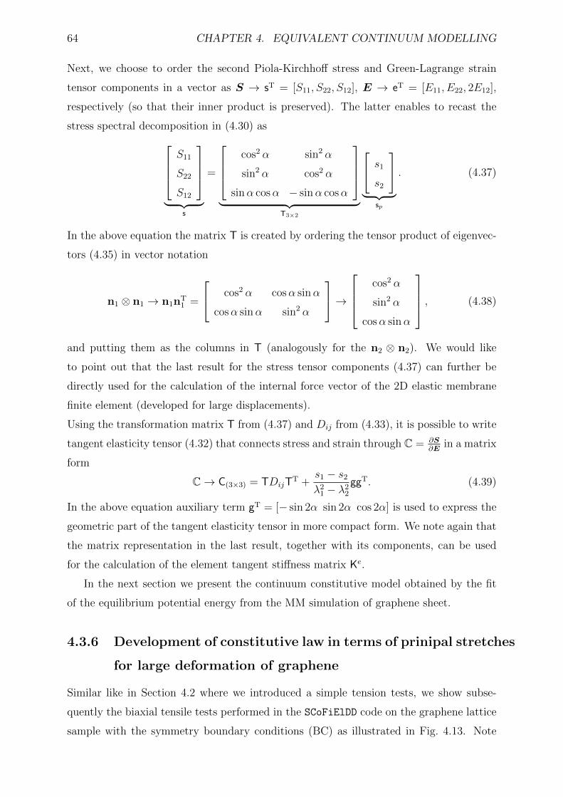
64 CHAPTER 4. EQUIVALENT CONTINUUM MODELLING
Next, we choose to order the second Piola-Kirchhoff stress and Green-Lagrange strain
tensor components in a vector as S → sT = [S11, S22, S12], E → eT = [E11, E22, 2E12],
respectively (so that their inner product is preserved). The latter enables to recast the
stress spectral decomposition in (4.30) asS11
S22
S12
︸ ︷︷ ︸
s
=
cos2 α sin2 α
sin2 α cos2 α
sinα cosα − sinα cosα
︸ ︷︷ ︸
T3×2
s1
s2
︸ ︷︷ ︸
sp
. (4.37)
In the above equation the matrix T is created by ordering the tensor product of eigenvec-
tors (4.35) in vector notation
n1 ⊗ n1 → n1nT1 =
cos2 α cosα sinα
cosα sinα sin2 α
→
cos2 α
sin2 α
cosα sinα
, (4.38)
and putting them as the columns in T (analogously for the n2 ⊗ n2). We would like
to point out that the last result for the stress tensor components (4.37) can further be
directly used for the calculation of the internal force vector of the 2D elastic membrane
finite element (developed for large displacements).
Using the transformation matrix T from (4.37) and Dij from (4.33), it is possible to write
tangent elasticity tensor (4.32) that connects stress and strain through C = ∂S∂E
in a matrix
form
C→ C(3×3) = TDijTT +s1 − s2
λ21 − λ2
2
ggT. (4.39)
In the above equation auxiliary term gT = [− sin 2α sin 2α cos 2α] is used to express the
geometric part of the tangent elasticity tensor in more compact form. We note again that
the matrix representation in the last result, together with its components, can be used
for the calculation of the element tangent stiffness matrix Ke.
In the next section we present the continuum constitutive model obtained by the fit
of the equilibrium potential energy from the MM simulation of graphene sheet.
4.3.6 Development of constitutive law in terms of prinipal stretches
for large deformation of graphene
Similar like in Section 4.2 where we introduced a simple tension tests, we show subse-
quently the biaxial tensile tests performed in the SCoFiElDD code on the graphene lattice
sample with the symmetry boundary conditions (BC) as illustrated in Fig. 4.13. Note
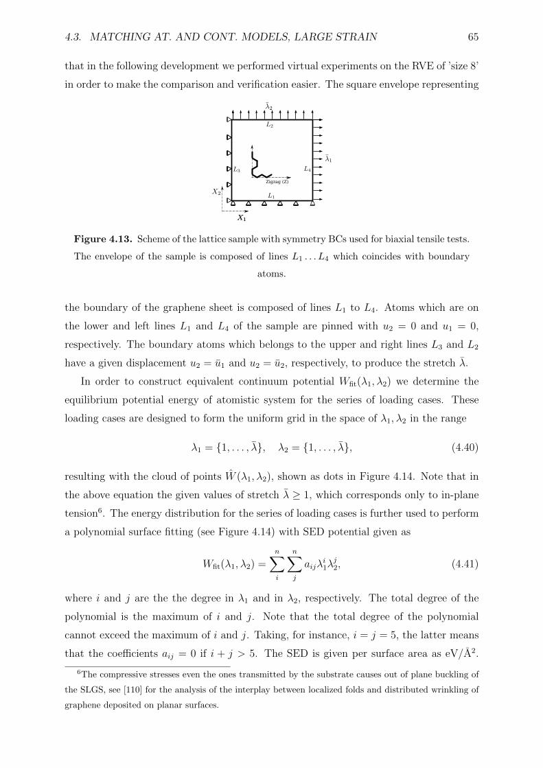
4.3. MATCHING AT. AND CONT. MODELS, LARGE STRAIN 65
that in the following development we performed virtual experiments on the RVE of ’size 8’
in order to make the comparison and verification easier. The square envelope representing
Zigzag (Z)
c)
Figure 4.13. Scheme of the lattice sample with symmetry BCs used for biaxial tensile tests.
The envelope of the sample is composed of lines L1 . . . L4 which coincides with boundary
atoms.
the boundary of the graphene sheet is composed of lines L1 to L4. Atoms which are on
the lower and left lines L1 and L4 of the sample are pinned with u2 = 0 and u1 = 0,
respectively. The boundary atoms which belongs to the upper and right lines L3 and L2
have a given displacement u2 = u1 and u2 = u2, respectively, to produce the stretch λ.
In order to construct equivalent continuum potential Wfit(λ1, λ2) we determine the
equilibrium potential energy of atomistic system for the series of loading cases. These
loading cases are designed to form the uniform grid in the space of λ1, λ2 in the range
λ1 = 1, . . . , λ, λ2 = 1, . . . , λ, (4.40)
resulting with the cloud of points W (λ1, λ2), shown as dots in Figure 4.14. Note that in
the above equation the given values of stretch λ ≥ 1, which corresponds only to in-plane
tension6. The energy distribution for the series of loading cases is further used to perform
a polynomial surface fitting (see Figure 4.14) with SED potential given as
Wfit(λ1, λ2) =n∑i
n∑j
aijλi1λ
j2, (4.41)
where i and j are the the degree in λ1 and in λ2, respectively. The total degree of the
polynomial is the maximum of i and j. Note that the total degree of the polynomial
cannot exceed the maximum of i and j. Taking, for instance, i = j = 5, the latter means
that the coefficients aij = 0 if i + j > 5. The SED is given per surface area as eV/A2.
6The compressive stresses even the ones transmitted by the substrate causes out of plane buckling of
the SLGS, see [110] for the analysis of the interplay between localized folds and distributed wrinkling of
graphene deposited on planar surfaces.
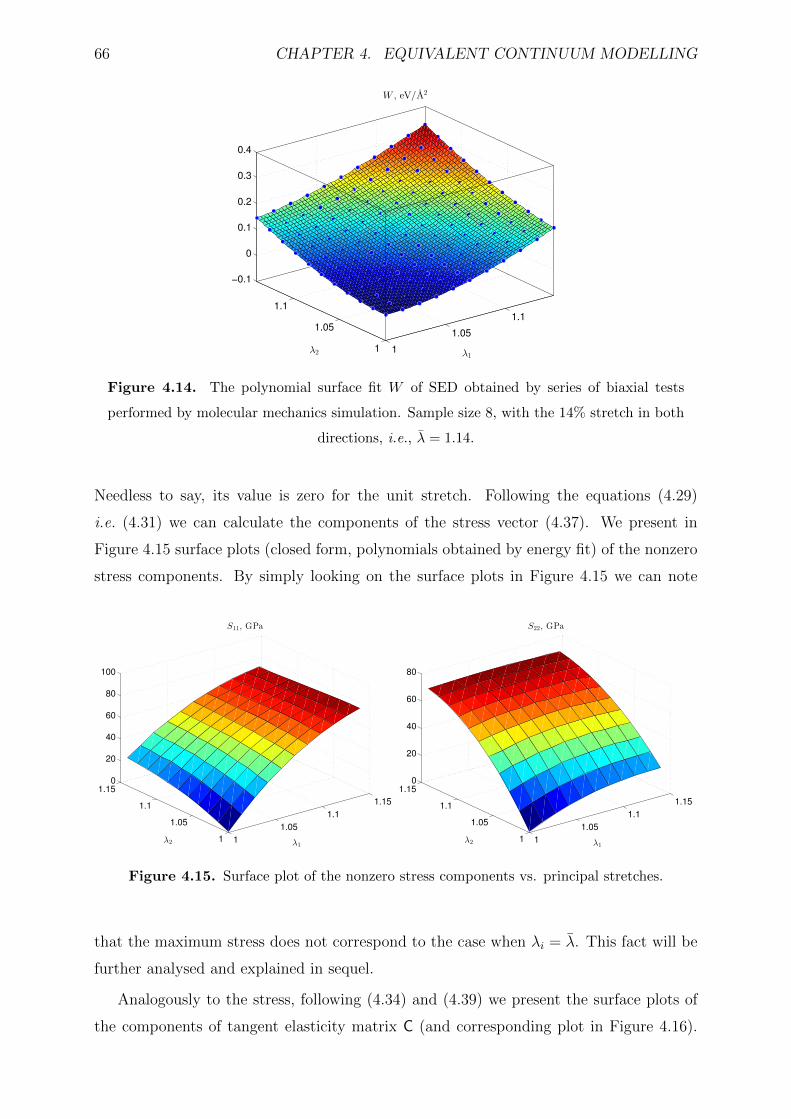
66 CHAPTER 4. EQUIVALENT CONTINUUM MODELLING
1
1.05
1.1
1
1.05
1.1
−0.1
0
0.1
0.2
0.3
0.4
λ1
W , eV/A2
λ2
Figure 4.14. The polynomial surface fit W of SED obtained by series of biaxial tests
performed by molecular mechanics simulation. Sample size 8, with the 14% stretch in both
directions, i.e., λ = 1.14.
Needless to say, its value is zero for the unit stretch. Following the equations (4.29)
i.e. (4.31) we can calculate the components of the stress vector (4.37). We present in
Figure 4.15 surface plots (closed form, polynomials obtained by energy fit) of the nonzero
stress components. By simply looking on the surface plots in Figure 4.15 we can note
1
1.05
1.1
1.15
1
1.05
1.1
1.15
0
20
40
60
80
100
λ1
S11, GPa
λ2 1
1.05
1.1
1.15
1
1.05
1.1
1.15
0
20
40
60
80
λ1
S22, GPa
λ2
Figure 4.15. Surface plot of the nonzero stress components vs. principal stretches.
that the maximum stress does not correspond to the case when λi = λ. This fact will be
further analysed and explained in sequel.
Analogously to the stress, following (4.34) and (4.39) we present the surface plots of
the components of tangent elasticity matrix C (and corresponding plot in Figure 4.16).
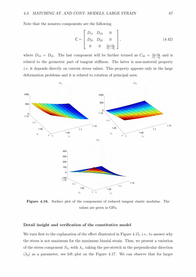
4.3. MATCHING AT. AND CONT. MODELS, LARGE STRAIN 67
Note that the nonzero components are the following
C =
D11 D12 0
D21 D22 0
0 0 s1−s2λ2
1−λ22
, (4.42)
where D12 = D21. The last component will be further termed as C33 = s1−s2λ2
1−λ22
and is
related to the geometric part of tangent stiffness. The latter is non-material property
i.e. it depends directly on current stress values. This property appears only in the large
deformation problems and it is related to rotation of principal axes.
1
1.05
1.1
1.15
1
1.05
1.1
1.15
0
500
1000
λ1
D11
λ2
1
1.05
1.1
1.15
1
1.05
1.1
1.15
0
500
1000
λ1
D22
λ2
1
1.05
1.1
1.15
1
1.05
1.1
1.15
−100
0
100
200
300
400
λ1
D12
λ2
Figure 4.16. Surface plot of the components of reduced tangent elastic modulus. The
values are given in GPa.
Detail insight and verification of the constitutive model
We turn first to the explanation of the effect illustrated in Figure 4.15, i.e., to answer why
the stress is not maximum for the maximum biaxial strain. Thus, we present a variation
of the stress component S11 with λ1, taking the pre-stretch in the perpendicular direction
(λ2) as a parameter, see left plot on the Figure 4.17. We can observe that for larger
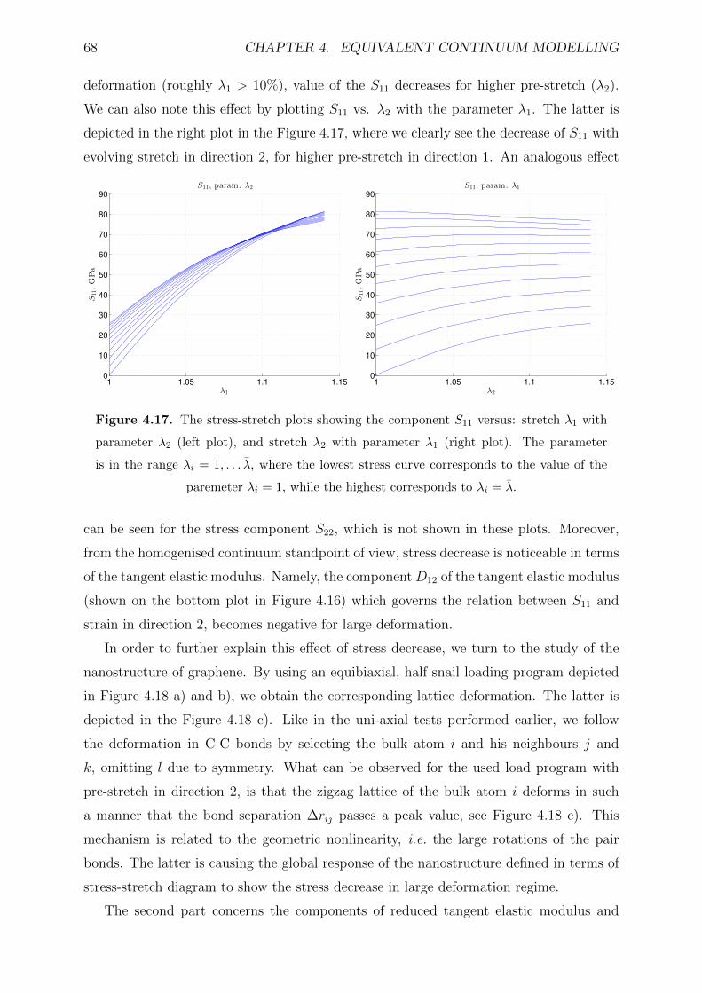
68 CHAPTER 4. EQUIVALENT CONTINUUM MODELLING
deformation (roughly λ1 > 10%), value of the S11 decreases for higher pre-stretch (λ2).
We can also note this effect by plotting S11 vs. λ2 with the parameter λ1. The latter is
depicted in the right plot in the Figure 4.17, where we clearly see the decrease of S11 with
evolving stretch in direction 2, for higher pre-stretch in direction 1. An analogous effect
1 1.05 1.1 1.150
10
20
30
40
50
60
70
80
90
S11, param. λ2
λ1
S11,GPa
1 1.05 1.1 1.150
10
20
30
40
50
60
70
80
90
S11, param. λ1
λ2
S11,GPa
Figure 4.17. The stress-stretch plots showing the component S11 versus: stretch λ1 with
parameter λ2 (left plot), and stretch λ2 with parameter λ1 (right plot). The parameter
is in the range λi = 1, . . . λ, where the lowest stress curve corresponds to the value of the
paremeter λi = 1, while the highest corresponds to λi = λ.
can be seen for the stress component S22, which is not shown in these plots. Moreover,
from the homogenised continuum standpoint of view, stress decrease is noticeable in terms
of the tangent elastic modulus. Namely, the component D12 of the tangent elastic modulus
(shown on the bottom plot in Figure 4.16) which governs the relation between S11 and
strain in direction 2, becomes negative for large deformation.
In order to further explain this effect of stress decrease, we turn to the study of the
nanostructure of graphene. By using an equibiaxial, half snail loading program depicted
in Figure 4.18 a) and b), we obtain the corresponding lattice deformation. The latter is
depicted in the Figure 4.18 c). Like in the uni-axial tests performed earlier, we follow
the deformation in C-C bonds by selecting the bulk atom i and his neighbours j and
k, omitting l due to symmetry. What can be observed for the used load program with
pre-stretch in direction 2, is that the zigzag lattice of the bulk atom i deforms in such
a manner that the bond separation ∆rij passes a peak value, see Figure 4.18 c). This
mechanism is related to the geometric nonlinearity, i.e. the large rotations of the pair
bonds. The latter is causing the global response of the nanostructure defined in terms of
stress-stretch diagram to show the stress decrease in large deformation regime.
The second part concerns the components of reduced tangent elastic modulus and
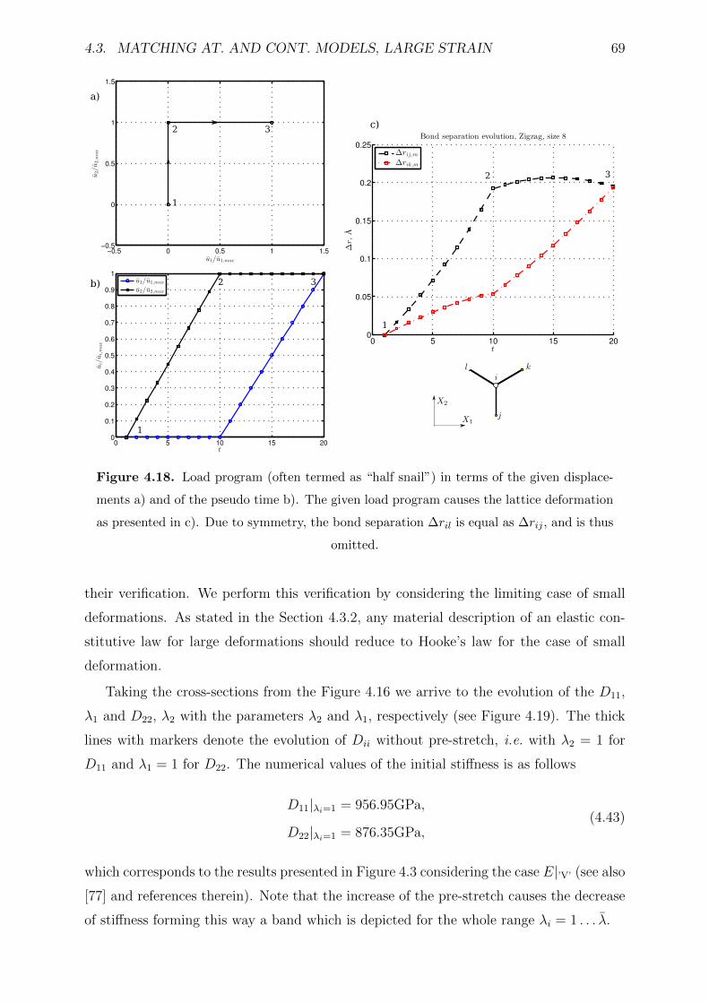
4.3. MATCHING AT. AND CONT. MODELS, LARGE STRAIN 69
1
2 3
a)
b)
c)
1
2 3
1
2 3
Figure 4.18. Load program (often termed as “half snail”) in terms of the given displace-
ments a) and of the pseudo time b). The given load program causes the lattice deformation
as presented in c). Due to symmetry, the bond separation ∆ril is equal as ∆rij , and is thus
omitted.
their verification. We perform this verification by considering the limiting case of small
deformations. As stated in the Section 4.3.2, any material description of an elastic con-
stitutive law for large deformations should reduce to Hooke’s law for the case of small
deformation.
Taking the cross-sections from the Figure 4.16 we arrive to the evolution of the D11,
λ1 and D22, λ2 with the parameters λ2 and λ1, respectively (see Figure 4.19). The thick
lines with markers denote the evolution of Dii without pre-stretch, i.e. with λ2 = 1 for
D11 and λ1 = 1 for D22. The numerical values of the initial stiffness is as follows
D11|λi=1 = 956.95GPa,
D22|λi=1 = 876.35GPa,(4.43)
which corresponds to the results presented in Figure 4.3 considering the case E|’V’ (see also
[77] and references therein). Note that the increase of the pre-stretch causes the decrease
of stiffness forming this way a band which is depicted for the whole range λi = 1 . . . λ.
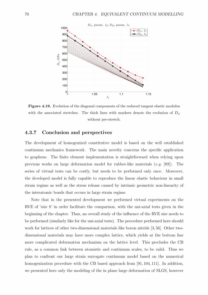
70 CHAPTER 4. EQUIVALENT CONTINUUM MODELLING
1 1.05 1.1 1.150
100
200
300
400
500
600
700
800
900
1000
D11, param. λ2; D22, param. λ1
λi
Dii,GPa
D11, λ1
D22, λ2
Figure 4.19. Evolution of the diagonal components of the reduced tangent elastic modulus
with the associated stretches. The thick lines with markers denote the evolution of Dii
without pre-stretch.
4.3.7 Conclusion and perspectives
The development of homogenized constitutive model is based on the well established
continuum mechanics framework. The main novelty concerns the specific application
to graphene. The finite element implementation is straightforward when relying upon
previous works on large deformation model for rubber-like materials (e.g. [89]). The
series of virtual tests can be costly, but needs to be performed only once. Moreover,
the developed model is fully capable to reproduce the linear elastic behaviour in small
strain regime as well as the stress release caused by intrinsic geometric non-linearity of
the interatomic bonds that occurs in large strain regime.
Note that in the presented development we performed virtual experiments on the
RVE of ’size 8’ in order facilitate the comparison, with the uni-axial tests given in the
beginning of the chapter. Thus, an overall study of the influence of the RVE size needs to
be performed (similarly like for the uni-axial tests). The procedure performed here should
work for lattices of other two-dimensional materials like boron nitride [3,56]. Other two-
dimensional materials may have more complex lattice, which yields at the bottom line
more complicated deformation mechanism on the lattice level. This precludes the CB
rule, as a common link between atomistic and continuum scales, to be valid. Thus we
plan to confront our large strain surrogate continuum model based on the numerical
homogenization procedure with the CB based approach from [91, 104, 111]. In addition,
we presented here only the modeling of the in plane large deformation of SLGS, however

4.3. MATCHING AT. AND CONT. MODELS, LARGE STRAIN 71
the extension to axisymmetric (like the CNT) or arbitrary curved membrane is possible
(see e.g. [112]), and will be concerned in future research.

72 CHAPTER 4. EQUIVALENT CONTINUUM MODELLING
Chapter 5Multiscale atomistic-to-continuum methods
for the simulation of graphene
For increased computational affordability, continuum models of graphene have become
attractive substitutes for MM simulations. The continuum model pertains to a consti-
tutive law, as described in previous chapter for small and large strain regime, and also
in [91, 103, 104]. These models usually incorporate interaction potentials into the con-
tinuum constitutive laws by homogenization through the Cauchy-Born rule or virtual
experiments and can reproduce the corresponding atomistic models of pristine graphene
with reasonable accuracy for smooth deformations.
However, continuum methods alone are not adequate for the analysis of defected graphene,
nor for bond failure analysis (see [49,51,52,58,113]). The limitations which are present in
both atomistic as well as continuum mechanics (CM) have stimulated extensive research
into MS methods that bridge atomistic simulation and continuum description. The fact
that fully atomistic model represents a heavy computational burden, together with the
assumption that the calculation of specific quantities of the solution can be accurately
approximated by replacing the particle model by a coarser model, is the basis for MS
modeling.
The idea is to use atomistic representations only in the localized region in which the
position of each individual atom is important and to use coarse-grained representations,
such as CM combined with the FE method, where the deformation is homogeneous and
smooth. Thus, this approach allows us to have the model of the atomistic lattice con-
structed at two scales: macro-scale that represents the homogenized behaviour of material
for computing the global structural response, and micro-scale that allows us to capture
the fine details of graphene microstructure (i.e. the behaviour of every single bond). The
73
74 CHAPTER 5. MS ATC METHODS FOR THE SIMULATION OF GRAPHENE
latter is in this work used to model the process of deformation of lattice defects. As will be
shown later in this chapter, this coupling method can reproduce the corresponding atom-
istic model reasonably well, but greatly reduces the number of unknowns in the nonlinear
system of equations.
The main focus and the purpose of this chapter is upon the interplay between the
atomistic model for graphene and the corresponding homogenised model placed in the
continuum mechanics framework. This is presented in the following layout. We give a brief
overview of the MS methods pointing out the differences between them. Next we focus on
the QC and BD methods giving the detail description and recent advances. We present the
comparison of the two methods in terms of the adaptive features (with the performance
comparison shown on the 1D examples) and coupling. A unified interpretation of the
coupling is proposed. In conclusion, the performance of the developed model is shown on
the real example of cracked graphene sheet.
5.1 A brief review of the atomistic-to-continuum MS
methods
Extensive work has been done in the development of atomistic-to-continuum MS mod-
elling approaches, starting with early works by Mullins and Dokainish (1982.) [114] and
Kohlhoff et al. (1990.) [115]. Mullins simulated 2D cracks in B.C.C crystal (i.e. α-iron)
in the context of a quasi static calculation with the atomic scale models, and due to
the restrictions of the computational power the question was how to connect the atomic
model and surrounding continuum. The basic idea is that the stresses are evaluated from
the interatomic potential under the imposing strains stemming from the FE nodal dis-
placements. Furthermore, these stresses are translated into nodal forces. Kohlhoff et al.
proposed somewhat new method for combined FE and atomistic analysis of crystal de-
fects, called FEAt. Here, an atomistic model is surrounded by a FE mesh with a small
overlap region enforcing boundary condition on the atomistic as well as on the contin-
uum domain. In particular, the authors of [115] tried to overcome the capturing problem
described in [114] by a refinement of the FE mesh down to the atomic scale with nodal
positions dictated by the crystal lattice structure. However, both early works dealt with
the problem of proper treatment of the transition between the lattice and continuum.
These early works initiated the further development of a great number of MS methods,
see e.g. some of the reviews in [23, 24, 26, 29, 30, 116, 117]. Numerous developed methods
appear at first, and from the theoretical standpoint of view, very different. However, as
5.1. A BRIEF REVIEW OF THE ATOMISTIC-TO-CONTINUUM MS METHODS 75
shown in [28], at the implementation level all these methods are very similar. In [28]
the comparison of the performance of a number of methods in a linear regime on a
common benchmark test is presented. The unified framework, available computer code,
and a quantitative comparison between the methods offer an exhaustive overview. Most
frequently used methods mentioned in these overviews are:
• quasicontinuum (QC) method (in Section 5.2),
• bridging domain/Arlequin method (often abbreviated as BD or BD/A, see Section
5.3),
• concurrent coupling of length scales (CLS) [27],
• bridging scale (BS) method [25,118,119],
• coupled atomistics and discrete dislocations (CADD) [120],
• atomistic-to-continuum coupling (AtC) [121–123],
• macroscopic (FE), atomistic (MD), ab-initio (TB) dynamics (MAAD) [124–126].
This list is by no means exhaustive. For instance, there is a recent effort of coupling
non-local to local continuum [127] in the Arlequin framework (see Section 5.3). An alter-
native to discrete modeling of atomic/particle systems is the use of non-local continuum
mechanics models (NLCM) [128]. NLCM reduces the computational costs but retains
the ability to capture non-local interactions. However, the simulation using NLCM is
also costly due to assembly operation of the discretized model where each point interacts
with multiple neighbours. The latter reduces the sparsity of the matrices and a similar
principle of coupling non-local continuum model with the local one is used.
We proceed with the generalisation of the differences between the most common MS
methods. In summary, various MS methods differ in:
1. the energy or force based formulation,
2. the coupling boundary conditions,
3. the existence of the handshake region,
4. and the choice of the continuum model.
76 CHAPTER 5. MS ATC METHODS FOR THE SIMULATION OF GRAPHENE
Formulation
There are two different approaches to finding equilibrium in quasi-static application. The
first, energy-based, is related to the minimisation of the total potential energy of the
system. The derivatives of the total energy in the energy-based approach lead to forces
on each atom/node which are necessarily zeroed when the energy is minimized. The
force-based approach considers the development of the physically motivated set of forces
on all degrees of freedom, and reach equilibrium by driving these forces to zero. However
these are not the same as the forces obtained from the energy potential. Thus, the two
approaches may seem as though they are equivalent, but they are not [28]. The force-
based approach facilitate the reduction of the perturbation (called ghost forces) in the
coupling area, but has no well-defined total energy. Note that both of the methods that we
focus upon, QC and BD, are energy based. Thus, the two methods do not differ in terms
of formulation (Ad 1), however in terms of other points (2 to 4) they differ significantly.
Coupling conditions
The coupling boundary conditions are related to the way the atomistic and continuum
degrees of freedom are connected. In general this can be done in a strong or weak form.
The former simply means gluing the atoms on the continuum which literally forces the
deformation of the atoms to be equal as the one defined by the interpolation in the
continuum. The latter considers coupling in the average sense. Both of the options will be
discussed herein, together with the option of coupling only displacement or displacement
and strains.
Handshake region
The fundamental idea of the handshake region is to provide a gradual transition from the
atomistic to continuum model. However this region is treated very differently in different
coupled models. In fact in some MS methods this region does not really exist, which is
often referred to as surface coupling. In others, a handshake region exists and represents
a partial overlap of the atomistic and continuum domains. In this zone the blending of the
continuum and atomistic descriptions is achieved. The latter is termed volume coupling
and considers overlapped domain decomposition. Both will be discussed here in terms of
QC and BD methods, respectively.
5.2. QUASICONTINUUM METHOD 77
Continuum model
The continuum part is usually treated with FEs. Note that there is also a number of works
about atomistic-to-continuum coupling when the continuum domain is treated with mesh-
less approach, see e.g. [129–131]. The details of the FE formulation and the constitutive
law adopted to describe the material response differ among the mentioned methods. In
some cases, a simple small strain finite element formulation is used with a linear elastic
model with elastic constants fitted to the properties of the atomistic model. In others,
a nonlinear finite strain formulation is used to describe the constitutive response in the
nonlinear range. We refer to both in this thesis, however due to simplicity in the MS
examples to follow we will use linear elastic continuum in small strain regime.
In the sequel the QC and the BD/A methods are described in more detail. The goal is,
however, to show the evolution of the BD/Arlequin coupling approach and to compare the
features regarding ability to adapt. Namely, the standard approach in BD method (as well
as in majority of the others) is to a priori identify the atomistic and continuum regions
and tie them together with some appropriate coupling (boundary) conditions. In addition
to the disadvantage of introducing artificial numerical interfaces into the problem a further
drawback of many of these models is their inability to adapt to changes in loading and
an evolving state of deformation. Take for example the problem of nanoindentation. As
the loading progresses and dislocations are emitted under the indenter the computational
model must be able to adapt and change in accordance with these new circumstances.
These aspects are intrinsic in QC method, i.e. it is one of the basic building blocks (see
next section). Thus, we will use it as the reference in respect of adaptivity.
5.2 Quasicontinuum method
The Quasicontinuum (QC) method is originally proposed in late 90’s by Tadmor, Ortiz
and Phillips [32]. Since then it has seen a great deal of development and application by a
number of researchers. The QC method has been used to study a variety of fundamental
aspects of deformation in crystalline solids, including fracture [132–134]1, grain boundary
slip and deformation [135]. The nano-indentation [136] and similar applications are exam-
ples where neither atomistic simulation nor continuum mechanics alone were appropriate,
whereas the QC was able to effectively combine the advantages of both models. The main
1In [132,133] the QC method has been applied to crack tip deformation and it accounted for both the
brittle fracture and ductile crack tip dislocation emission.
78 CHAPTER 5. MS ATC METHODS FOR THE SIMULATION OF GRAPHENE
goal of the QC method is to provide a seamless link of the atomistic and continuum scales.
The energy of the coupled system consists of the energy of both domains. However, in
QC the conceptual advantage in developing the coupled energy equation pertains to the
fact that there is no distinction between atoms and nodes. This goal is achieved by the
three main building blocks [137,138]:
1. Reduction of degrees of freedom (DOF) by coarse-graining of fully atomistic reso-
lution via kinematic constraints. The fully atomistic description is retained only in
the regions of interest.
2. An approximation of the energy in the coarse grained region via numerical quadra-
ture. The main idea is to avoid the need to calculate the energy of all the atoms,
but retain only a few so-called rep-atoms.
3. Ability of the fully refined, atomistic region to evolve with deformation, where adap-
tivity is directed by suitable refinement indicator.
5.2.1 DOF reduction or coarse graining
If the deformation changes gradually on the atomistic scale, it is not necessary to explicitly
track the displacement of every atom in the region. Instead it is sufficient to consider some
selected atoms, often called representative atoms or rep-atoms. This process is in essence
the upscaling via coarse graining. Only rep-atoms have independent DOF while all other
atoms are forced to follow the interpolated motion of the rep-atoms. The QC incorporates
such a scheme by means of the interpolation functions of the FE method, and thus the FE
triangulation has to be performed with rep-atoms as FE mesh nodes. This way continuum
assumption is implicitly introduced in QC method.
Let the total potential energy Etot be given as a function of displacement u (similarly as
in (3.1))
Etot(u) = U(u)−N∑i=1
fiui, (5.1)
where fi is the external force on the atom i and U is an atomistic internal energy, i.e. the
energy stored in atomistic bonds, see (3.8). For the sake of derivation we repeat (3.10)
where the internal energy is expressed as the sum of atom energies (Ei)
U =N∑i=1
Ei(u). (5.2)
5.2. QUASICONTINUUM METHOD 79
Next, the kinematic constraint described above is accomplished by replacing U with Uh
Uh =N∑i=1
Ei(uh), (5.3)
where uh is the approximated displacement field. The displacement approximation is
given via standard FE interpolation
uh =
Nrep∑i=1
Niui, (5.4)
where Ni is a shape function and ui is the displacement for the node/rep-atom i. Clearly,
the constraints introduced by the interpolation of the displacements is some level of ap-
proximation. The density of rep-atoms vary in space according to the considered problem.
In the vicinity of region of interest every atom is considered as rep-atom (fully refined)
and in region of more slowly varying deformation gradient, only a few atoms are chosen.
5.2.2 Efficient energy calculation via Cauchy-Born rule, local
QC
Described kinematic constraint on most of the atoms in the body will achieve the goal of
reducing the number of degrees of freedom in the problem. However, for the purpose of
energy minimization the energy of all the atoms (not just rep-atoms) has to be computed.
The way to avoid visiting every atom is the Cauchy-Born (CB) rule [86,87,139]. The CB
rule postulates that when a simple, mono-atomic crystal is subjected to small displacement
on its boundary then all the atoms will follow this displacement. In QC this rule is
implemented in that every atom in a region subject to a uniform deformation gradient
will be energetically equivalent. Thus, energy within an element e can be estimated
by computing the energy of one, single atom in the deformed state. The estimation is
performed simply by multiplying the single atom energy by the number of atoms in the
element e.
Let F be the deformation gradient and E0 the energy of the unit cell when its lattice
vectors are distorted according to the given deformation gradient. The strain energy
density (SED) of the element can then be expressed as:
W (F ) =E0(F )
Ω0
, (5.5)
where Ω0 is the volume of the unit cell. Having this result in hand, the sum in eq. (5.3)
where i = 1 . . . N is reduced to number of FEs (Nelem) as
Uh ≈ Uh′ =
Nelem∑e=1
ΩeW (F e). (5.6)
80 CHAPTER 5. MS ATC METHODS FOR THE SIMULATION OF GRAPHENE
In the above equation, the element volume and unit cell volume are related as neΩ0 = Ωe,
and ne is the number of atoms contained in element e. Using the CB rule, the QC can
be thought of as a purely continuum formulation (local QC), but with a constitutive law
that is based on atomistic model rather than on an assumed phenomenological form [138].
Within QC framework, the calculation of CB energy is done separately in a subroutine.
For a given deformation gradient F the lattice vectors in a unit cell are deformed according
to given F and the SED is obtained according to eq. (5.5). The main limitation pertaining
to the CB rule is that it is valid only for simple lattices. Virtual experiments performed in
Chapter 4 do not have this limitation. In the original QC formulation the constant strain
triangle (CST) elements (2D) are used with the linear shape functions to interpolate
the displacement field within each element. In this case the deformation gradient is
uniform. This boils down to the following: the Cauchy-Born rule assumes that a uniform
deformation gradient at the macro-scale can be mapped directly to the same uniform
deformation on the micro-scale. The latter will be used further for the unified coupling
formulation.
5.2.3 Non-local QC and local/non-local coupling
In settings where the deformation is varying slowly and the FE size is adequate with
respect to the variations of the deformation, the local QC is sufficiently accurate and
very effective. In the non-local regions, which can be eventually refined to fully atomistic
resolution, the energy in (5.3) can be calculated by explicitly computing the energy of the
rep-atoms by numerical quadrature
Uh ≈ Uh′ =
Nrep∑i=1
niEi(uh), (5.7)
where ni is the weight for the rep-atom i. The value of the weight is high for rep-atoms
in regions of low rep-atom density, and low for the region of the high density. Thus, ni is
the number of the atoms represented by the i-th rep-atom with the limiting case of ni = 1
for fully atomistic region and consistency requirement
Nrep∑i=1
ni = N. (5.8)
The main advantage of the non-local QC is that when it is refined down to the atomic
scale, it reduces exactly to lattice statics, given in (3.1).
High accuracy of non-local formulation can be combined with the high efficiency of the
local formulation. Needless to say, non-local formulation is employed in the region where
5.2. QUASICONTINUUM METHOD 81
atomic scale accuracy is needed, and local where the deformation is changing relatively
slow. Thus, the rep-atom can be chosen as local or non-local depending on its deformation
environment giving Nrep = Nloc +Nnonloc. The total energy (5.3) is then approximated as
Uh =
Nnonloc∑i=1
niEi(uh) +
Nloc∑i=1
niEi(uh), (5.9)
The above equation is yet another way of writing that the internal energy of the coupled
system is a sum of atomistic (non-local) and continuum (local, here CB-based) energies,
respectively.
Regarding the calculation of the weights ni in the above equation, for both local or non-
local rep-atom, the Voronoi tessellation is used, i.e. the cells around each rep-atom. Let
the cell of atom i contains ni atoms, and nei of these atoms reside in FE e adjacent to
rep-atom i. The weighted energy contribution of rep-atom i is then found by applying
the CB rule within each element adjacent to i such that
niEi =
N iel∑e
niΩ0cW (F e), ni =
N iel∑e
nei , (5.10)
where Ω0c is the cell volume for single atom, and N iel is the number of FE adjacent to
atom i.
5.2.4 Local/non-local criterion
The criterion to trigger the non-local treatment is based on the significant variation of de-
formation gradient2. Precisely, we say that the state of deformation near a representative
atom is nearly homogeneous if the deformation gradients that it senses from the different
surrounding elements are nearly equal. The non-locality criterion is then:
maxa,b,k|λak − λbk| < εc, (5.11)
where λak is the k-th eigenvalue of the right stretch tensor for element a, k = 1 . . . 3 and
indices a and b (a 6= b) refers to the neighboring elements of rep-atom. The rep-atom will
be made local if this inequality is satisfied, and non-local otherwise, depending on the
empirical constant εc.
2Note that simply having a large deformation in a region does not in itself require a non-local rep-
atom, as the CB rule of the local formulation will exactly describe the energy of any uniform deformation,
regardless of its size.
82 CHAPTER 5. MS ATC METHODS FOR THE SIMULATION OF GRAPHENE
5.2.5 Adaptivity
Without a priori knowledge of where the deformation field will require fine-scale resolu-
tion, it is necessary that the method should have a built-in, automatic way to adapt the
finite element mesh through the addition or removal of rep-atoms. This is a feature that
is in QC inherent from the FE literature, where considerable attention has been given
to adaptive meshing techniques for many years, e.g. [140]. Typically in FE techniques, a
scalar measure is defined to quantify the error introduced into the solution by the cur-
rent density of nodes (or rep-atoms in the QC). Elements in which this error estimator
is higher than some prescribed tolerance are targeted for adaptation, while at the same
time the error estimator can be used to remove unnecessary nodes from the model.
The error estimator in terms of deformation gradient is defined as the difference
between the actual solution and the estimate of the higher order (index ’ho’) solution
(see [138])
εeF =
√1
Ωe
∫Ωe
(F ho − F e)2dΩe, (5.12)
where Ωe is the volume of the FE e, F e is the solution for the deformation gradient
in element e, and F ho = NF avg is the higher order estimate obtained by interpolating
nodal values F avg, which simply represents the average of the deformation gradients of
the elements touching the given node. If this error is small, it implies that the higher
order solution is well represented by the lower order elements in the region, and thus
no refinement is required. Needless to say, elements for which the error is greater than
some prescribed error tolerance are targeted for refinement. Refinement then proceeds by
adding three new rep-atoms at the atomic sites closest to the mid-sides of the targeted
elements (the constant strain triangle (CST) elements are used). If the nearest atomic
sites to the mid-sides of the elements are the atoms at the element corners, the region is
fully refined and no new rep-atoms can be added. The same error estimator is used in
the QC to remove unnecessary rep-atoms from the mesh. In this process, a rep-atom is
temporarily removed from the mesh and the surrounding region is locally re-meshed (i.e.
nodal connectivity table is rebuilt). If all of the elements produced by this re-meshing
process have a value of the error estimator below the threshold, the rep-atom can be
eliminated. Essentially, the idea is to examine the necessity of each node. To prevent
excessive coarsening of the mesh far from defects the nodes corresponding to the initial
mesh are usually protected from deletion [135].
With these ideas in hand we turn to introduce the BD method. Note that initially
emphasis of the research related to atomistic-to-continuum MS methods, namely BD
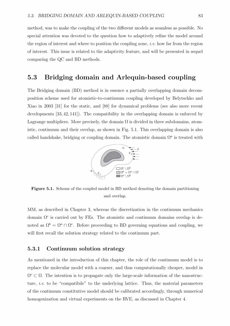
5.3. BRIDGING DOMAIN AND ARLEQUIN-BASED COUPLING 83
method, was to make the coupling of the two different models as seamless as possible. No
special attention was devoted to the question how to adaptively refine the model around
the region of interest and where to position the coupling zone, i.e. how far from the region
of interest. This issue is related to the adaptivity feature, and will be presented in sequel
comparing the QC and BD methods.
5.3 Bridging domain and Arlequin-based coupling
The Bridging domain (BD) method is in essence a partially overlapping domain decom-
position scheme used for atomistic-to-continuum coupling developed by Belytschko and
Xiao in 2003 [31] for the static, and [88] for dynamical problems (see also more recent
developments [33, 42, 141]). The compatibility in the overlapping domain is enforced by
Lagrange multipliers. More precisely, the domain Ω is divided in three subdomains, atom-
istic, continuum and their overlap, as shown in Fig. 5.1. This overlapping domain is also
called handshake, bridging or coupling domain. The atomistic domain Ωa is treated with
Figure 5.1. Scheme of the coupled model in BD method denoting the domain partitioning
and overlap.
MM, as described in Chapter 3, whereas the discretization in the continuum mechanics
domain Ωc is carried out by FEs. The atomistic and continuum domains overlap is de-
noted as Ωb = Ωa ∩ Ωc. Before proceeding to BD governing equations and coupling, we
will first recall the solution strategy related to the continuum part.
5.3.1 Continuum solution strategy
As mentioned in the introduction of this chapter, the role of the continuum model is to
replace the molecular model with a coarser, and thus computationally cheaper, model in
Ωc ⊂ Ω. The intention is to propagate only the large-scale information of the nanostruc-
ture, i.e. to be “compatibile” to the underlying lattice. Thus, the material parameters
of the continuum constitutive model should be calibrated accordingly, through numerical
homogenization and virtual experiments on the RVE, as discussed in Chapter 4.
84 CHAPTER 5. MS ATC METHODS FOR THE SIMULATION OF GRAPHENE
The deformable solid body is considered as a collection of particles, where the posi-
tion of each particle is denoted with X in reference and with x in current configuration.
The displacement vector is given as u(X) = x − X. We consider further in the pre-
sented numerical examples the geometrically linear theory of solid mechanics. Thus we
assume the hypothesis of small displacement gradients ‖∇u(X)‖ 1, which allows us
to use symmetric part of displacement gradient tensor as appropriate strain measure,
ε = 12(∇u +∇uT ). The kinematic hypothesis on small displacement gradients allows us
to parametrize volume and surface forces and stress with respect to the coordinates in the
initial configuration. This choice of continuum is used due to the coupling formulation
described next. Moreover, since the substitute model is used only far from the region of
interest, the continuum model is used only in the zone of homogeneous and small defor-
mation. The region of interest is considered as the region in the vicinity of the lattice
defect, as the crack-like presented in the numerical examples.
Let W (ε(X),X) represent the continuum potential in terms of SED, which for the case
of hyperelasticity allows us to compute the stress tensor as
σ =∂W (ε(X))
∂ε. (5.13)
We consider Hook’s law where SED is given as
W =1
2ε(X) · C(X)ε(X), (5.14)
where C is elasticity tensor that can be also expressed as C = ∂2W (·)∂ε2
. The parameters of
this elasticity tensor are calibrated by homogenisation, as described in Chapter 4.
We now construct the weak form of the continuum boundary value problem in Ωc,
satisfying the equilibrium only in average sense. We assume that Dirichlet boundary
conditions u = u are prescribed on the part Γu of the boundary Γ. The nanostruc-
ture system represented as continuum is in general subjected to tractions t on the part
Γσ of the boundary and to a volume forces b in Ω. We introduce the space of ad-
missible solutions V = u ∈ H1(Ω); u = u on Γu and space of virtual displacement field
V0 = v ∈ H1(Ω); v = 0 on Γu. This choice of real and virtual displacement fields ensur-
ing sufficient regularity (u,w ∈ H1(Ω)) should also satisfy the weak form of equilibrium
equation
0 = G(u; v) :=
∫Ω
∇sv · σ(∇su)dΩ−∫
Ω
v · bdΩ−∫
Γσ
v · tdΓ, (5.15)
where ∇s(·) = sym[∇(·)]. Under the assumption of hyperelastic material with (5.13) and
(5.14), the weak form in (5.15) is identical (see e.g. [10]) to the condition of the minimum
5.3. BRIDGING DOMAIN AND ARLEQUIN-BASED COUPLING 85
of the total potential energy, given as
Ectot :=
∫Ω
W (∇su)dΩ−∫
Ω
u · bdΩ−∫
Γσ
u · tdΓ. (5.16)
The weak form given in (5.15) is used as the basis for constructing the finite element
approximation. In this work, we used first the 1D truss, isoparametric finite element with
2 nodes (nn = 2) for the parametric study on the chain-like model. Next, for the MS
modeling of defected graphene the quadrilateral isoparametric finite element (Q4) with
nn = 4 is used. By choosing the so called isoparamtric FEs (see e.g. [10,78,140]) the same
shape functions (Na) are used for geometry representation and for the construction of
the discrete approximations of the real and virtual displacement fields. In the case of Q4
FE, the displacement field uh is constructed by employing the bilinear shape functions
Na (e.g. see [10])
uh|Ωe =4∑
a=1
Nauea; uh ∈ Vh. (5.17)
The virtual field is constructed analogously, with the same shape functions
vh|Ωe =4∑
a=1
Navea; vh ∈ Vh0 . (5.18)
In (5.17) above uea are the nodal displacement values related to element e, and Vh ⊂ V ,
which implies that the displacement field remains kinematically admissible. Analogously
in (5.18) for the approximation of virtual displacement vh ∈ Vh0 and Vh0 ⊂ V0, with the zero
nodal values on the Dirichlet boundary. The discrete approximation of the infinitesimal
strain field (∇su = ε) is
εh|Ωe =4∑
a=1
Bauea, (5.19)
where Ba are the derivatives of the shape functions. The analogy for the virtual strain
field is valid. Considering (5.13) and proposed approximation, the stress values can be
computed from the SED as
σh =∂W (εh)
∂εh. (5.20)
By exploiting these results, i.e. by introducing the displacement and strain approximations
in the weak form of equilibrium equation3 (5.15), we can easily obtain the element stiffness
matrix.
3By introducing the displacement and strain approximations in the weak form of equilibrium equation
we arrive to the well know Galerkin equation. Considering that the values of the virtual displacement is
arbitrary on the free nodes, the well known equation in the form Kd = f is obtained.
86 CHAPTER 5. MS ATC METHODS FOR THE SIMULATION OF GRAPHENE
5.3.2 Governing equations and coupling
In QC method the total potential energy is composed of local and non-local parts, which
correspond to continuum and atomistic description. This approach somewhat hides the
true coupling between the two descriptions. In BD method the system can be clearly
decomposed into continuum and atomistic parts which are glued together. Thus, the
total potential energy (with index w denoting that the energy term is weighted in Ωb) of
the system considering (3.1) and (5.16) may be written as
Etot,w = Eatot,w(d) + Ec
tot,w(u), (5.21)
where d and u are displacement vectors in the atomistic and continuum domains, respec-
tively. The weighted atomistic and continuum energies are defined as
Eatot,w =
∑i
(∑j 6=i
waijVp +∑j 6=k 6=i
wai Vθ
)−∑i∈Ωa
wai fi · di, (5.22)
Ectot,w =
∫Ωcwc(X)WdΩc −
∫Ωcwc(X)u · bdΩc −
∫Γcσ
wc(X)u · tdΓc, (5.23)
where Vp and Vθ are given in general for the modified Morse potential (3.28). In the
bridging domain the two models overlap, and the weighting functions wa and wc in (5.22)
and (5.23) partition the energy. The weighting function serves to blend the behaviour
from the continuum model (wc) and the atomistic model (wa) and to avoid the double
counting of the energy in the bridging domain. More importantly, the use of an overlap-
ping subdomain obviates the need for the FE nodes of the continuum model to correspond
to the atomic positions. The weighting functions wc and wa define a partition of unity of
the energy in the bridging domain as follows:
wc(X) = 1 for X ∈ Ωc \ Ωb,
wa(X) = 1 for X ∈ Ωa \ Ωb, (5.24)
wc(X) + wa(X) = 1 for X ∈ Ωb.
The energy weighting functions are usually taken to be constant, linear (ramp) or cubic
functions of X in Ωb.
The Lagrange multiplier (LM) method is used to achieve the coupling and later to
convert the problem of constrained minimization into finding the energy minimum of the
larger, unconstrained problem. Thus, we introduce the space of LM as M = H1(Ωb),
and denote LM with λ ∈M. In order to enforce the compatibility between the atomistic
and continuum domains, the coupling term C in terms of energy is added to total energy
5.3. BRIDGING DOMAIN AND ARLEQUIN-BASED COUPLING 87
forming so called Lagrangian
WL := Etot,w + C. (5.25)
The choice of the coupling term determines which quantities and in which fashion should
be coupled. Namely, we can choose whether only displacement or both the displacement
and the displacement gradients are coupled. We will present two types: the strong (or
discrete), and weak coupling. In the former, coupling of the atomistic and continuum
models is achieved by enforcing (only) displacement compatibility in the bridging domain
as u(X = Xi) = di, ∀i ∈ Ωb. The compatibility constraint between each atomistic
displacement (discrete) and the continuum displacement field can be written as [31,33]
C1 :=∑i∈Ωb
∫Ωbλ(X) · [u(X)− di] δ(X−Xi)dΩ, (5.26)
where δ(·) is Dirac’s delta function. Note that the right hand side in the above equation
is left in the integral form because the Lagrange multipliers will be approximated as a
field.
The evolution of the BD method has much in common with recent works in the FE
community on the coupling of nonconforming meshes in the overlapping subdomain. This
approach is known as Arlequin method developed by Ben Dhia [35] (see also [142, 143]).
The same Arlequin approach is lately also applied for atomistic-to-continuum coupling,
see [34, 36–39, 41, 44]. In the Arlequin method the coupling is given in the weak sense.
This coupling can be generalised as
C2 :=
∫Ωbα1λ · (u− db) + α2∇λ(∇u−∇db)dΩ, (5.27)
where the choice of the weighting parameters α1 and α2 determines the coupling by mix-
ing the displacement and strain coupling terms, and db(X) is the interpolated atomistic
displacement field in Ωb. The two versions of coupling, named L2 and H1, are obtained
for the value of the weighting given (α1, α2) = (1, 0), and (α1, α2) = (1, 1), respectively.
Note also, that the names L2 and H1, originate from the fact that they define the scalar
products in Lebesgue (L2) and Sobolev (H1) spaces [35], respectively. Thus, the latter
can be defined as
(λ,u− db)L2 :=
∫Ωbλ · (u− db)dΩ, (5.28)
(λ,u− db)H1 :=
∫Ωbλ · (u− db) + l2∇λ(∇u−∇db)dΩ, (5.29)
where l is simply the length of the bridging zone. Needless to say, an interpolated atomic
displacement field is needed for this formulation of coupling, as well as its derivative. In
88 CHAPTER 5. MS ATC METHODS FOR THE SIMULATION OF GRAPHENE
this thesis, the interpolation of the discrete atom displacement is obtained by interpolant
(Φ) based on moving least squares (MLS) approximation [33,34], which gives
db(X) = Φdi = NmlsD−1di ∀i ∈ Ωb, (5.30)
where Nmls is the matrix of the MLS shape functions, and D is the matrix that has the
values of the MLS shape functions at the atom position in Ωb. The latter is introduced
since the MLS approximation does not interpolate the approximated field (i.e. it lacks
the kronecker delta property Nmlsi (Xj) 6= δij), see Appendix B for details.
Having these results in hand, we present next the weak form of the coupling problem.
In the Chapter 3 we introduced Va and Va0 to be the sets of trial (d) and test (w) functions
in Ωa, respectively. Analogously, for the continuum domain we have introduced the space
of admissible solutions V and the space of test functions V0. Let us also denote the space
of LM withM = λ,µ ∈ H1(Ω). We further proceed to the minimising of the functional
in (5.25) with the coupling term defined as (5.27), i.e. (5.28) or (5.29). This leads to the
saddle point problem, which can be written in terms of its weak form:
Find (u,d,λ) ∈ V × Va ×M such that
Gcw(u; v) +Ga
w(d; w) + (λ,v − Φwi|i∈Ωb
)L2 or H1 = 0 ∀(v,w) ∈ V0 × Va0 ,
(µ,u− db)L2 or H1 = 0 ∀µ ∈M, (5.31)
where the terms defining the weak form of equilibrium with the scaling in the overlap are
as follows
Gcw(u; v) :=
∫Ωcwc∇sv · σ(∇su)dΩ−
∫Ωcwcv · bdΩ−
∫Γcσ
wcv · tdΓ, (5.32)
Gaw(d; w) :=
∑i∈Ωa
(∑j 6=i
waij∂Vp∂di·wi +
∑j 6=k 6=i
wai∂Vθ∂di·wi
)−∑i∈Ωa
wai fi ·wi. (5.33)
Next we will present the numerical implementation of the given coupling formulation
with the coupling term C2 given in (5.27). We thus introduce LM FE field approximation
with corresponding shape functions Nλa as
λh|Ωe =
nλ∑a=1
Nλaλ
ea; λh ∈Mh ⊂M, (5.34)
where nλ is the number of nodal points of the FE used to approximate LM field. The
λea = [λe1 λe2]T denotes the unknown nodal values in terms of LMs. By introducing the
displacement and strain approximations (equatoins (5.17), (5.19) and analogous for the
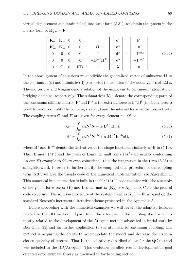
5.3. BRIDGING DOMAIN AND ARLEQUIN-BASED COUPLING 89
virtual displacement and strain fields) into weak form (5.31), we obtain the system in the
matrix form of KgU = F
Kcc Kcb 0 0 0
KTcb Kbb 0 0 GT
0 0 0 0 0
0 0 0 0 −D−THT
0 G 0 −HD−1 0
uc
ub
da
db
λ
=
Fc
0
−f int,a
−f int,b
0
. (5.35)
In the above system of equations we subdivide the generalized vector of unknowns U to
the continuum (u) and atomistic (d) parts with the addition of the nodal values of LM’s.
The indices c, a and b again denote relation of the unknowns to continuum, atomistic or
bridging domains, respectively. The submatrices K(··) denote the corresponding parts of
the continuum stiffness matrix, Fc and f int is the external force in Ωc\Ωb (the body force b
is set to zero to simplify the coupling strategy) and the internal force vector, respectively.
The coupling terms G and H are given for every element e ∈ Ωb as
Ge =
∫Ωeα1N
λN + α2Bλ,TBdΩ, (5.36)
He =
∫Ωeα1N
λNmls + α2Bλ,TBmlsdΩ, (5.37)
where Bλ and Bmls denote the derivatives of the shape functions, similarly as B in (5.19).
The FE mesh (M c) and the mesh of Lagrange multipliers (Mλ) are usually conforming
(in our 2D example to follow even coincident), thus the integration in the term (5.36) is
straightforward. In order to further clarify the computational procedure of the coupling
term (5.37) we give the pseudo code of the numerical implementation, see Algorithm 1.
This numerical implementation is built in the SCoFiElDD code together with the assembly
of the global force vector (F) and Hessian matrix (Kg), see Appendix C for the general
code structure. The solution procedure of the system given as KgU = F, is based on the
standard Newton’s incremental-iterative scheme presented in the Appendix A.
Before proceeding with the numerical examples we will revisit the adaptive features
related to the BD method. Apart from the advances in the coupling itself which is
mostly related to the development of the Arlequin method advocated in initial work by
Ben Dhia [35] and its further application to the atomistic-to-continuum coupling, this
method is acquiring the ability to accommodate the model and decrease the error in
chosen quantity of interest. That is, the adaptivity described above for the QC method
was included in the BD/Arlequin. This evolution parallels recent development in goal
oriented error estimate theory as discussed in forthcoming section.
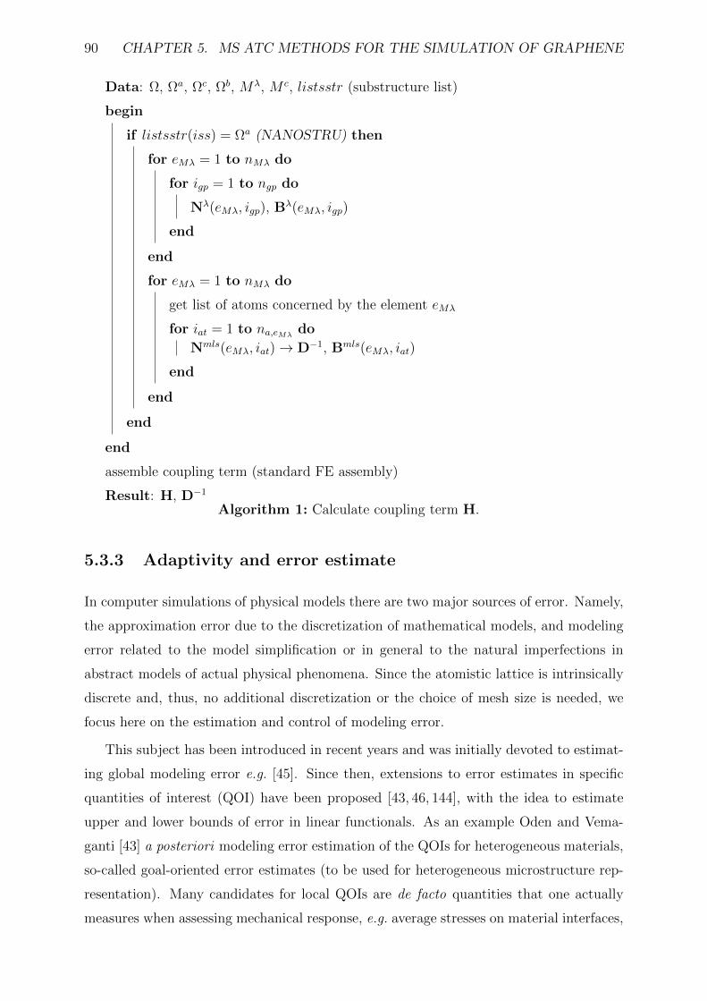
90 CHAPTER 5. MS ATC METHODS FOR THE SIMULATION OF GRAPHENE
Data: Ω, Ωa, Ωc, Ωb, Mλ, M c, listsstr (substructure list)
begin
if listsstr(iss) = Ωa (NANOSTRU) then
for eMλ = 1 to nMλ do
for igp = 1 to ngp do
Nλ(eMλ, igp), Bλ(eMλ, igp)
end
end
for eMλ = 1 to nMλ do
get list of atoms concerned by the element eMλ
for iat = 1 to na,eMλdo
Nmls(eMλ, iat)→ D−1, Bmls(eMλ, iat)
end
end
end
end
assemble coupling term (standard FE assembly)
Result: H, D−1
Algorithm 1: Calculate coupling term H.
5.3.3 Adaptivity and error estimate
In computer simulations of physical models there are two major sources of error. Namely,
the approximation error due to the discretization of mathematical models, and modeling
error related to the model simplification or in general to the natural imperfections in
abstract models of actual physical phenomena. Since the atomistic lattice is intrinsically
discrete and, thus, no additional discretization or the choice of mesh size is needed, we
focus here on the estimation and control of modeling error.
This subject has been introduced in recent years and was initially devoted to estimat-
ing global modeling error e.g. [45]. Since then, extensions to error estimates in specific
quantities of interest (QOI) have been proposed [43, 46, 144], with the idea to estimate
upper and lower bounds of error in linear functionals. As an example Oden and Vema-
ganti [43] a posteriori modeling error estimation of the QOIs for heterogeneous materials,
so-called goal-oriented error estimates (to be used for heterogeneous microstructure rep-
resentation). Many candidates for local QOIs are de facto quantities that one actually
measures when assessing mechanical response, e.g. average stresses on material interfaces,
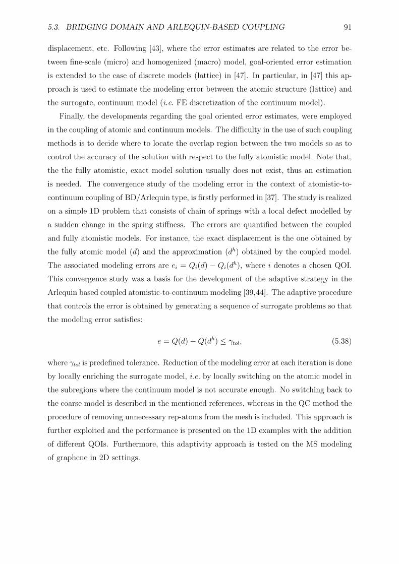
5.3. BRIDGING DOMAIN AND ARLEQUIN-BASED COUPLING 91
displacement, etc. Following [43], where the error estimates are related to the error be-
tween fine-scale (micro) and homogenized (macro) model, goal-oriented error estimation
is extended to the case of discrete models (lattice) in [47]. In particular, in [47] this ap-
proach is used to estimate the modeling error between the atomic structure (lattice) and
the surrogate, continuum model (i.e. FE discretization of the continuum model).
Finally, the developments regarding the goal oriented error estimates, were employed
in the coupling of atomic and continuum models. The difficulty in the use of such coupling
methods is to decide where to locate the overlap region between the two models so as to
control the accuracy of the solution with respect to the fully atomistic model. Note that,
the the fully atomistic, exact model solution usually does not exist, thus an estimation
is needed. The convergence study of the modeling error in the context of atomistic-to-
continuum coupling of BD/Arlequin type, is firstly performed in [37]. The study is realized
on a simple 1D problem that consists of chain of springs with a local defect modelled by
a sudden change in the spring stiffness. The errors are quantified between the coupled
and fully atomistic models. For instance, the exact displacement is the one obtained by
the fully atomic model (d) and the approximation (dh) obtained by the coupled model.
The associated modeling errors are ei = Qi(d) − Qi(dh), where i denotes a chosen QOI.
This convergence study was a basis for the development of the adaptive strategy in the
Arlequin based coupled atomistic-to-continuum modeling [39,44]. The adaptive procedure
that controls the error is obtained by generating a sequence of surrogate problems so that
the modeling error satisfies:
e = Q(d)−Q(dh) ≤ γtol, (5.38)
where γtol is predefined tolerance. Reduction of the modeling error at each iteration is done
by locally enriching the surrogate model, i.e. by locally switching on the atomic model in
the subregions where the continuum model is not accurate enough. No switching back to
the coarse model is described in the mentioned references, whereas in the QC method the
procedure of removing unnecessary rep-atoms from the mesh is included. This approach is
further exploited and the performance is presented on the 1D examples with the addition
of different QOIs. Furthermore, this adaptivity approach is tested on the MS modeling
of graphene in 2D settings.
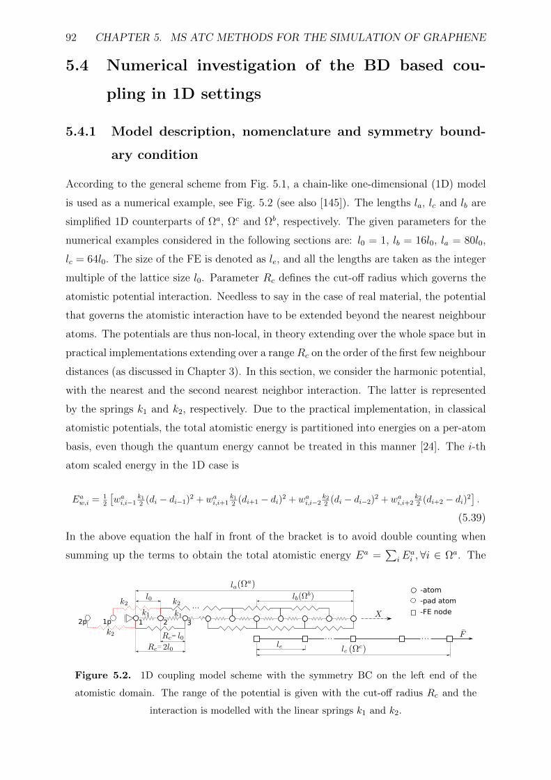
92 CHAPTER 5. MS ATC METHODS FOR THE SIMULATION OF GRAPHENE
5.4 Numerical investigation of the BD based cou-
pling in 1D settings
5.4.1 Model description, nomenclature and symmetry bound-
ary condition
According to the general scheme from Fig. 5.1, a chain-like one-dimensional (1D) model
is used as a numerical example, see Fig. 5.2 (see also [145]). The lengths la, lc and lb are
simplified 1D counterparts of Ωa, Ωc and Ωb, respectively. The given parameters for the
numerical examples considered in the following sections are: l0 = 1, lb = 16l0, la = 80l0,
lc = 64l0. The size of the FE is denoted as le, and all the lengths are taken as the integer
multiple of the lattice size l0. Parameter Rc defines the cut-off radius which governs the
atomistic potential interaction. Needless to say in the case of real material, the potential
that governs the atomistic interaction have to be extended beyond the nearest neighbour
atoms. The potentials are thus non-local, in theory extending over the whole space but in
practical implementations extending over a range Rc on the order of the first few neighbour
distances (as discussed in Chapter 3). In this section, we consider the harmonic potential,
with the nearest and the second nearest neighbor interaction. The latter is represented
by the springs k1 and k2, respectively. Due to the practical implementation, in classical
atomistic potentials, the total atomistic energy is partitioned into energies on a per-atom
basis, even though the quantum energy cannot be treated in this manner [24]. The i-th
atom scaled energy in the 1D case is
Eaw,i = 1
2
[wai,i−1
k1
2(di − di−1)2 + wai,i+1
k1
2(di+1 − di)2 + wai,i−2
k2
2(di − di−2)2 + wai,i+2
k2
2(di+2 − di)2
].
(5.39)
In the above equation the half in front of the bracket is to avoid double counting when
summing up the terms to obtain the total atomistic energy Ea =∑
iEai ,∀i ∈ Ωa. The
...
...
...
. ..
-atom
-FE node
-pad atom
1p2p 1 2 3
Figure 5.2. 1D coupling model scheme with the symmetry BC on the left end of the
atomistic domain. The range of the potential is given with the cut-off radius Rc and the
interaction is modelled with the linear springs k1 and k2.
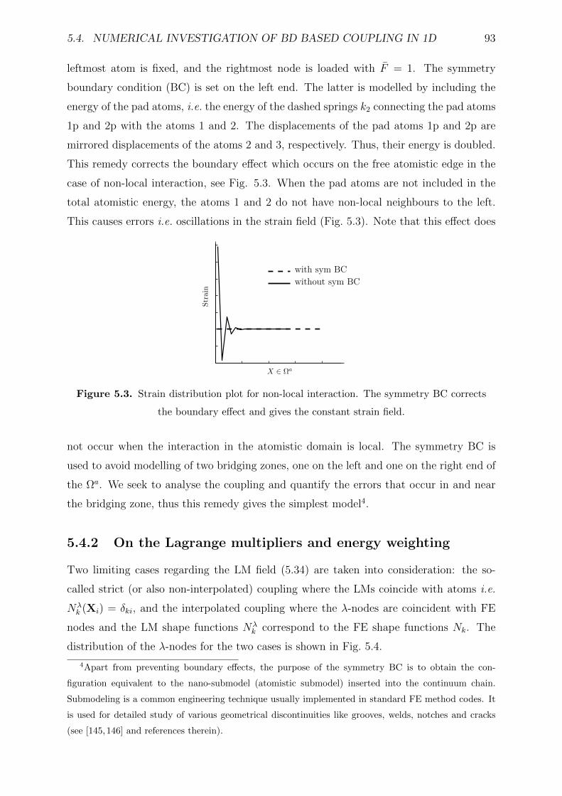
5.4. NUMERICAL INVESTIGATION OF BD BASED COUPLING IN 1D 93
leftmost atom is fixed, and the rightmost node is loaded with F = 1. The symmetry
boundary condition (BC) is set on the left end. The latter is modelled by including the
energy of the pad atoms, i.e. the energy of the dashed springs k2 connecting the pad atoms
1p and 2p with the atoms 1 and 2. The displacements of the pad atoms 1p and 2p are
mirrored displacements of the atoms 2 and 3, respectively. Thus, their energy is doubled.
This remedy corrects the boundary effect which occurs on the free atomistic edge in the
case of non-local interaction, see Fig. 5.3. When the pad atoms are not included in the
total atomistic energy, the atoms 1 and 2 do not have non-local neighbours to the left.
This causes errors i.e. oscillations in the strain field (Fig. 5.3). Note that this effect does
with sym BC
without sym BC
Figure 5.3. Strain distribution plot for non-local interaction. The symmetry BC corrects
the boundary effect and gives the constant strain field.
not occur when the interaction in the atomistic domain is local. The symmetry BC is
used to avoid modelling of two bridging zones, one on the left and one on the right end of
the Ωa. We seek to analyse the coupling and quantify the errors that occur in and near
the bridging zone, thus this remedy gives the simplest model4.
5.4.2 On the Lagrange multipliers and energy weighting
Two limiting cases regarding the LM field (5.34) are taken into consideration: the so-
called strict (or also non-interpolated) coupling where the LMs coincide with atoms i.e.
Nλk (Xi) = δki, and the interpolated coupling where the λ-nodes are coincident with FE
nodes and the LM shape functions Nλk correspond to the FE shape functions Nk. The
distribution of the λ-nodes for the two cases is shown in Fig. 5.4.
4Apart from preventing boundary effects, the purpose of the symmetry BC is to obtain the con-
figuration equivalent to the nano-submodel (atomistic submodel) inserted into the continuum chain.
Submodeling is a common engineering technique usually implemented in standard FE method codes. It
is used for detailed study of various geometrical discontinuities like grooves, welds, notches and cracks
(see [145,146] and references therein).
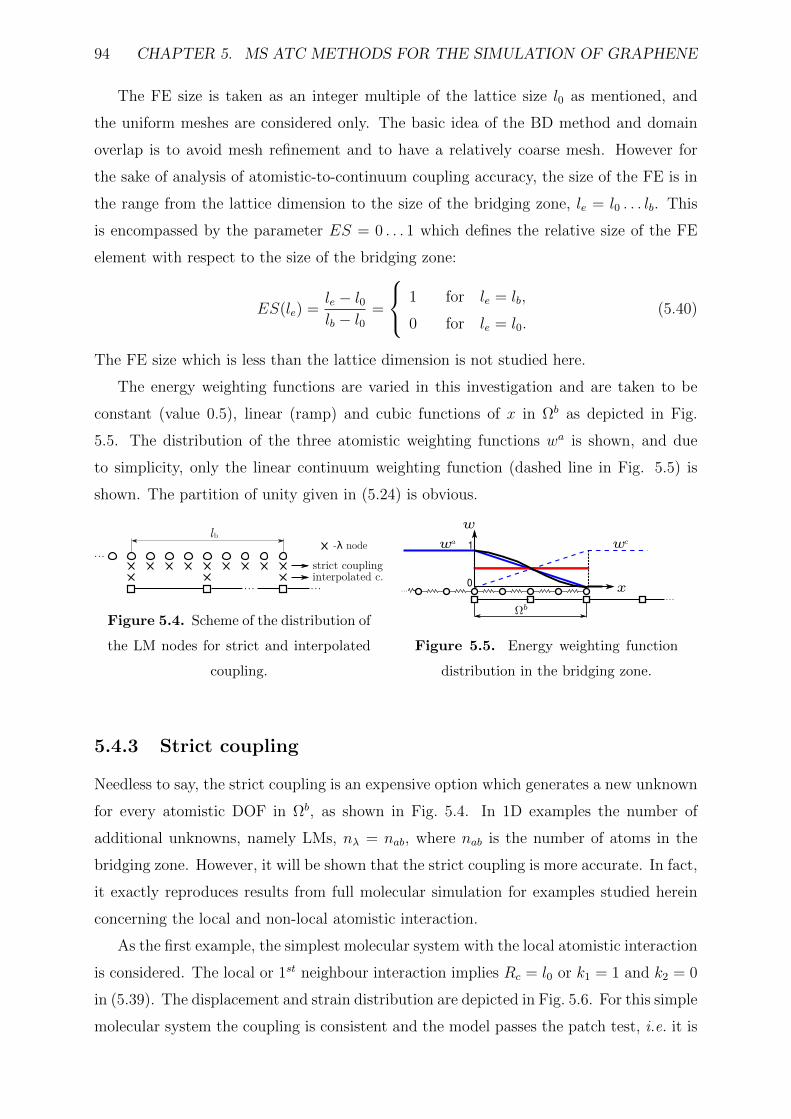
94 CHAPTER 5. MS ATC METHODS FOR THE SIMULATION OF GRAPHENE
The FE size is taken as an integer multiple of the lattice size l0 as mentioned, and
the uniform meshes are considered only. The basic idea of the BD method and domain
overlap is to avoid mesh refinement and to have a relatively coarse mesh. However for
the sake of analysis of atomistic-to-continuum coupling accuracy, the size of the FE is in
the range from the lattice dimension to the size of the bridging zone, le = l0 . . . lb. This
is encompassed by the parameter ES = 0 . . . 1 which defines the relative size of the FE
element with respect to the size of the bridging zone:
ES(le) =le − l0lb − l0
=
1 for le = lb,
0 for le = l0.(5.40)
The FE size which is less than the lattice dimension is not studied here.
The energy weighting functions are varied in this investigation and are taken to be
constant (value 0.5), linear (ramp) and cubic functions of x in Ωb as depicted in Fig.
5.5. The distribution of the three atomistic weighting functions wa is shown, and due
to simplicity, only the linear continuum weighting function (dashed line in Fig. 5.5) is
shown. The partition of unity given in (5.24) is obvious.
...
lb
...
strict coupling interpolated c.
-λ node...
Figure 5.4. Scheme of the distribution of
the LM nodes for strict and interpolated
coupling.
...
...
1wa
wc
0x
w
Figure 5.5. Energy weighting function
distribution in the bridging zone.
5.4.3 Strict coupling
Needless to say, the strict coupling is an expensive option which generates a new unknown
for every atomistic DOF in Ωb, as shown in Fig. 5.4. In 1D examples the number of
additional unknowns, namely LMs, nλ = nab, where nab is the number of atoms in the
bridging zone. However, it will be shown that the strict coupling is more accurate. In fact,
it exactly reproduces results from full molecular simulation for examples studied herein
concerning the local and non-local atomistic interaction.
As the first example, the simplest molecular system with the local atomistic interaction
is considered. The local or 1st neighbour interaction implies Rc = l0 or k1 = 1 and k2 = 0
in (5.39). The displacement and strain distribution are depicted in Fig. 5.6. For this simple
molecular system the coupling is consistent and the model passes the patch test, i.e. it is
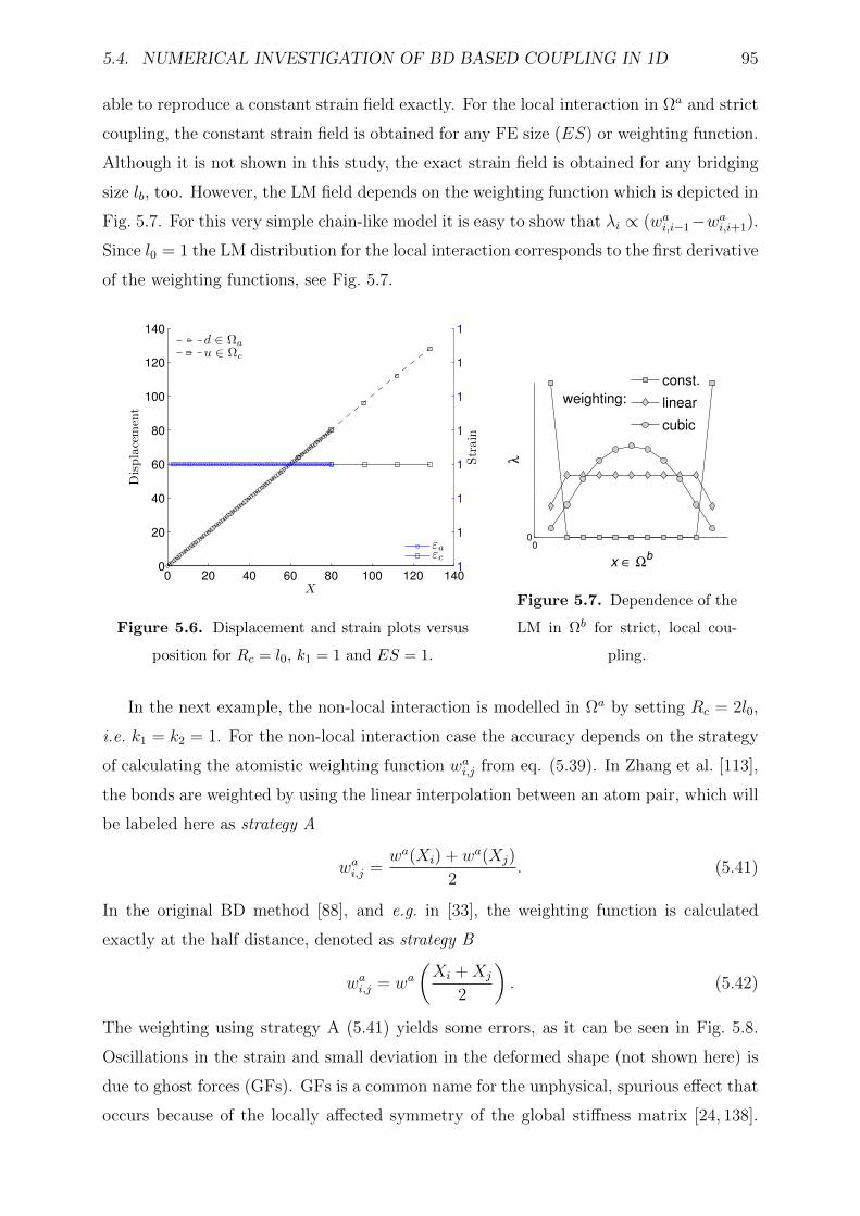
5.4. NUMERICAL INVESTIGATION OF BD BASED COUPLING IN 1D 95
able to reproduce a constant strain field exactly. For the local interaction in Ωa and strict
coupling, the constant strain field is obtained for any FE size (ES) or weighting function.
Although it is not shown in this study, the exact strain field is obtained for any bridging
size lb, too. However, the LM field depends on the weighting function which is depicted in
Fig. 5.7. For this very simple chain-like model it is easy to show that λi ∝ (wai,i−1−wai,i+1).
Since l0 = 1 the LM distribution for the local interaction corresponds to the first derivative
of the weighting functions, see Fig. 5.7.
0 20 40 60 80 100 120 1400
20
40
60
80
100
120
140
X
Displacement
d ∈ Ωau ∈ Ωc
1
1
1
1
1
1
1
1
Strain
εaεc
Figure 5.6. Displacement and strain plots versus
position for Rc = l0, k1 = 1 and ES = 1.
00
x ∈ Ωb
λ
const.
linear
cubic
weighting:
Figure 5.7. Dependence of the
LM in Ωb for strict, local cou-
pling.
In the next example, the non-local interaction is modelled in Ωa by setting Rc = 2l0,
i.e. k1 = k2 = 1. For the non-local interaction case the accuracy depends on the strategy
of calculating the atomistic weighting function wai,j from eq. (5.39). In Zhang et al. [113],
the bonds are weighted by using the linear interpolation between an atom pair, which will
be labeled here as strategy A
wai,j =wa(Xi) + wa(Xj)
2. (5.41)
In the original BD method [88], and e.g. in [33], the weighting function is calculated
exactly at the half distance, denoted as strategy B
wai,j = wa(Xi +Xj
2
). (5.42)
The weighting using strategy A (5.41) yields some errors, as it can be seen in Fig. 5.8.
Oscillations in the strain and small deviation in the deformed shape (not shown here) is
due to ghost forces (GFs). GFs is a common name for the unphysical, spurious effect that
occurs because of the locally affected symmetry of the global stiffness matrix [24, 138].
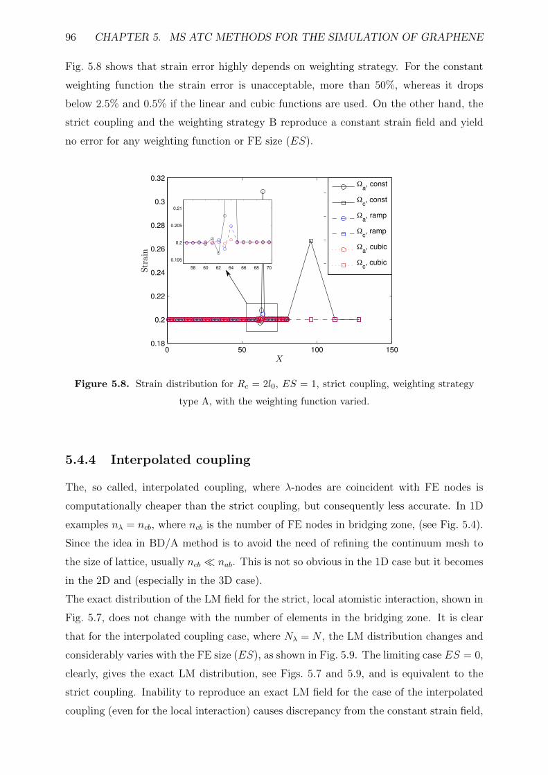
96 CHAPTER 5. MS ATC METHODS FOR THE SIMULATION OF GRAPHENE
Fig. 5.8 shows that strain error highly depends on weighting strategy. For the constant
weighting function the strain error is unacceptable, more than 50%, whereas it drops
below 2.5% and 0.5% if the linear and cubic functions are used. On the other hand, the
strict coupling and the weighting strategy B reproduce a constant strain field and yield
no error for any weighting function or FE size (ES).
Figure 5.8. Strain distribution for Rc = 2l0, ES = 1, strict coupling, weighting strategy
type A, with the weighting function varied.
5.4.4 Interpolated coupling
The, so called, interpolated coupling, where λ-nodes are coincident with FE nodes is
computationally cheaper than the strict coupling, but consequently less accurate. In 1D
examples nλ = ncb, where ncb is the number of FE nodes in bridging zone, (see Fig. 5.4).
Since the idea in BD/A method is to avoid the need of refining the continuum mesh to
the size of lattice, usually ncb nab. This is not so obvious in the 1D case but it becomes
in the 2D and (especially in the 3D case).
The exact distribution of the LM field for the strict, local atomistic interaction, shown in
Fig. 5.7, does not change with the number of elements in the bridging zone. It is clear
that for the interpolated coupling case, where Nλ = N , the LM distribution changes and
considerably varies with the FE size (ES), as shown in Fig. 5.9. The limiting case ES = 0,
clearly, gives the exact LM distribution, see Figs. 5.7 and 5.9, and is equivalent to the
strict coupling. Inability to reproduce an exact LM field for the case of the interpolated
coupling (even for the local interaction) causes discrepancy from the constant strain field,
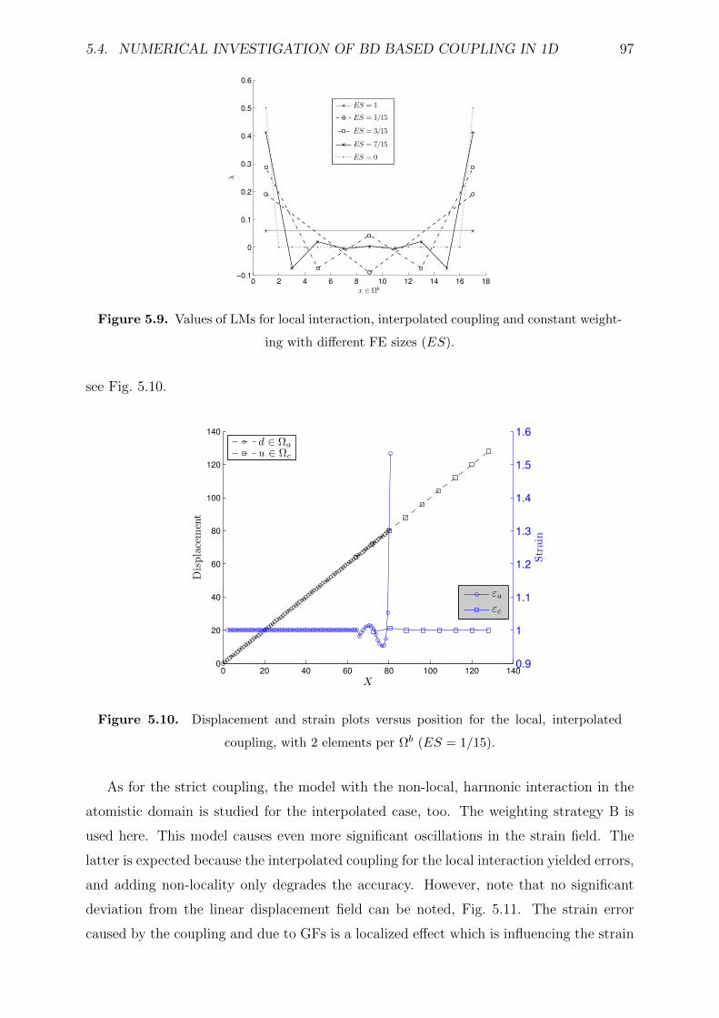
5.4. NUMERICAL INVESTIGATION OF BD BASED COUPLING IN 1D 97
Figure 5.9. Values of LMs for local interaction, interpolated coupling and constant weight-
ing with different FE sizes (ES).
see Fig. 5.10.
0 20 40 60 80 100 120 1400
20
40
60
80
100
120
140
X
Displacement
d ∈ Ωau ∈ Ωc
0.9
1
1.1
1.2
1.3
1.4
1.5
1.6
Strain
εaεc
Figure 5.10. Displacement and strain plots versus position for the local, interpolated
coupling, with 2 elements per Ωb (ES = 1/15).
As for the strict coupling, the model with the non-local, harmonic interaction in the
atomistic domain is studied for the interpolated case, too. The weighting strategy B is
used here. This model causes even more significant oscillations in the strain field. The
latter is expected because the interpolated coupling for the local interaction yielded errors,
and adding non-locality only degrades the accuracy. However, note that no significant
deviation from the linear displacement field can be noted, Fig. 5.11. The strain error
caused by the coupling and due to GFs is a localized effect which is influencing the strain
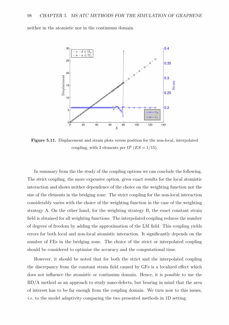
98 CHAPTER 5. MS ATC METHODS FOR THE SIMULATION OF GRAPHENE
neither in the atomistic nor in the continuum domain.
0 20 40 60 80 100 120 1400
5
10
15
20
25
30
X
Displacement
d ∈ Ωau ∈ Ωc
0.2
0.25
0.3
0.35
0.4
Strain
εaεc
Figure 5.11. Displacement and strain plots versus position for the non-local, interpolated
coupling, with 2 elements per Ωb (ES = 1/15).
In summary from the the study of the coupling options we can conclude the following.
The strict coupling, the more expensive option, gives exact results for the local atomistic
interaction and shows neither dependence of the choice on the weighting function nor the
size of the elements in the bridging zone. The strict coupling for the non-local interaction
considerably varies with the choice of the weighting function in the case of the weighting
strategy A. On the other hand, for the weighting strategy B, the exact constant strain
field is obtained for all weighting functions. The interpolated coupling reduces the number
of degrees of freedom by adding the approximation of the LM field. This coupling yields
errors for both local and non-local atomistic interaction. It significantly depends on the
number of FEs in the bridging zone. The choice of the strict or interpolated coupling
should be considered to optimize the accuracy and the computational time.
However, it should be noted that for both the strict and the interpolated coupling
the discrepancy from the constant strain field caused by GFs is a localized effect which
does not influence the atomistic or continuum domain. Hence, it is possible to use the
BD/A method as an approach to study nano-defects, but bearing in mind that the area
of interest has to be far enough from the coupling domain. We turn now to this issues,
i.e. to the model adaptivity comparing the two presented methods in 1D setting.
5.5. MS METHODS COMPARISON 99
5.5 MS methods comparison
5.5.1 General
In the foregoing, we have given an overview of the mainstream MS methods in terms of
QC method and BD/Arlequin based coupling. The latter currently attracts the greatest
attention with many recent developments, but it still has not been fully completed as the
simpler, but well known QC method. Therefore, we seek to summarize in this section
the comparison of these two methods, hoping to be able to draw lessons on further im-
provements to the present practise. This comparison is carried out regarding: 1. coupling
algorithm, 2. continuum modeling, 3. applicability, and finally 4. adaptivity.
Coupling algorithm
The coupling algorithms of these two methods seems to be drastically different. The
QC method seeks to provide a gradual transition, where the mesh composed of repatoms
as nodes is gradually refined starting from the local towards the non-local description.
This gradual transition is numerically more convenient regarding its capability to reduce
the ill-conditioning. However, this approach has the following drawbacks. Firstly, an
enormous refinement has to be performed in going from the FE continuum representation
to the atomistic lattice size. Furthermore, the FE nodes and the atoms have to coincide.
Contrary to that, BD/A method couples the two models only in the zone of partial overlap.
Neither gradual transition nor coincidence between the nodes and elements are needed.
The latter should enable to insert an atomistic patch almost anywhere in the structure,
without severely changing the continuum mesh. However, atomistic and continuum DOFs
are completely separated and additional unknowns in terms of Lagrange multipliers that
enforce the coupling need to be accounted for. In addition, in order to avoid double
counting the blending of the energy in overlapping domain is done by weighting functions,
which also have to be chosen appropriately.
Continuum modeling
QC method works with large deformation intrinsically. That is, CB rule is used for
continuum constitutive relation thus constitutive law is based on atomistics rather than
on an assumed phenomenological form. On the other hand, CB hypothesis is satisfied only
for simple lattice structures. Due to use of classical coupling of atomic and continuum
domains, in the BD/A method the surrogate continuum model is obtained by fitting the
100 CHAPTER 5. MS ATC METHODS FOR THE SIMULATION OF GRAPHENE
material parameters from virtual experiments on RVE. This approach obviates the need
for the CB hypothesis to be satisfied.
Applicability
During development period of the QC method, it served both as a key vehicle for un-
derstanding of the nature of atomistic-continuum coupling, and as a practical tool for
investigating problems requiring coupled atomistic-continuum solution procedure. Nowa-
days, there is a unified web site qcmethod.org as the original source of information, with
publications and the most important download section. Under the download section the
QC code is available written in Fortran90 by the Tadmor and Miller. The BD/A method
was less used as a practical tool, apart the application to CNT. It was, somewhat, more
used for the theoretical testing of different aspects of coupling and MS modeling in general.
However the method is from the very beginning extended to dynamics, dealing with spu-
rious wave reflections in the transition from the atomic to continuum domain. There is no
unified web site as for QC method, but there are examples like libmultiscale.gforge.inria.fr.
Adaptivity
Original QC method is in essence an adaptive FE approach, and adaptivity is intrinsically
in the formulation in QC method. BD/A method was initially assumed as approach to
couple two different models. Nevertheless, the described evolution associated with the
goal oriented error estimate theory, with the strong mathematical foundations, improved
the method so that it shows good performance in the sense of model adaptivity (compared
to the QC method). However, the choice where to place the fine and where to remain with
coarse scale model, and how to provide the appropriate evolution of that region is still the
most important question. Adaptivity driven by the described goals algorithm considers
controlling the model refinement with respect to any chosen QOI. In the QC method
non-locality criterion is based on a significant variation in the deformation gradient, no
other criteria was implemented.
The idea of model adaptivity is shown schematically in the Fig. 5.12 for the 1D case.
In the latter scheme we suppose that the strain field is perturbed in the left end of the
chain, and the adaptive procedure advances from some initial model shown on the top.
Even though this procedure for the QC approach looks similar to a mesh refinement, the
main goal is to address the possibility of model adaptivity in the terms of substitution of
the continuum model with the atomic one. As described in QC section, adapting process
in this method advances by selecting new atoms as rep-atoms/nodes in the area where
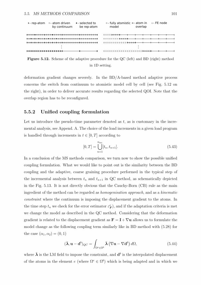
5.5. MS METHODS COMPARISON 101
...
- rep-atom - atom driven
by continuum
- selected to
be rep-atom
...
- fully atomistic
model
- atom in
overlap
- FE node
Figure 5.12. Scheme of the adaptive procedure for the QC (left) and BD (right) method
in 1D setting.
deformation gradient changes severely. In the BD/A-based method adaptive process
concerns the switch from continuum to atomistic model cell by cell (see Fig. 5.12 on
the right), in order to deliver accurate results regarding the selected QOI. Note that the
overlap region has to be reconfigured.
5.5.2 Unified coupling formulation
Let us introduce the pseudo-time parameter denoted as t, as is customary in the incre-
mental analysis, see Append. A. The choice of the load increments in a given load program
is handled through increments in t ∈ [0, T ] according to
[0, T ] =
ninc⋃n=1
[tn, tn+1]. (5.43)
In a conclusion of the MS methods comparison, we turn now to show the possible unified
coupling formulation. What we would like to point out is the similarity between the BD
coupling and the adaptive, coarse graining procedure performed in the typical step of
the incremental analysis between tn and tn+1 in QC method, as schematically depicted
in the Fig. 5.13. It is not directly obvious that the Cauchy-Born (CB) rule as the main
ingredient of the method can be regarded as homogenisation approach, and as a kinematic
constraint where the continuum is imposing the displacement gradient to the atoms. In
the time step tn we check for the error estimator εeF ), and if the adaptation criteria is met
we change the model as described in the QC method. Considering that the deformation
gradient is related to the displacement gradient as F = I +∇u allows us to formulate the
model change as the following coupling term similarly like in BD method with (5.28) for
the case (α1, α2) = (0, 1)
(λ,u− db)QC =
∫Ωe∈Ωb
λ(∇u−∇db
)dΩ, (5.44)
where λ is the LM field to impose the constraint, and db is the interpolated displacement
of the atoms in the element e (where Ωe ∈ Ωb) which is being adapted and in which we
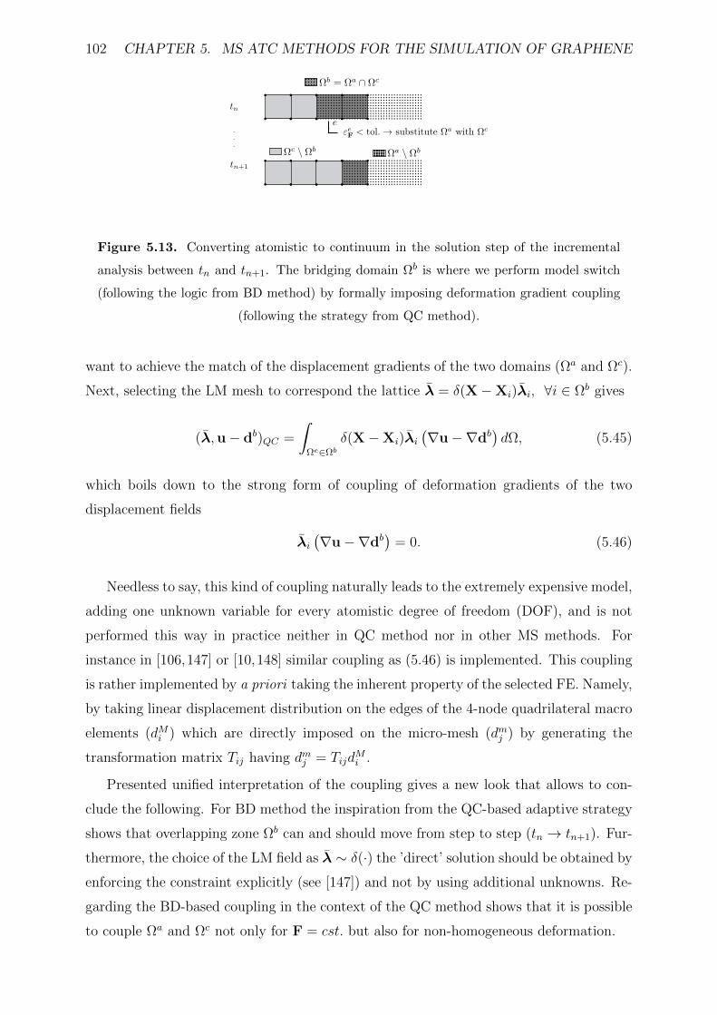
102 CHAPTER 5. MS ATC METHODS FOR THE SIMULATION OF GRAPHENE
.
.
.
Figure 5.13. Converting atomistic to continuum in the solution step of the incremental
analysis between tn and tn+1. The bridging domain Ωb is where we perform model switch
(following the logic from BD method) by formally imposing deformation gradient coupling
(following the strategy from QC method).
want to achieve the match of the displacement gradients of the two domains (Ωa and Ωc).
Next, selecting the LM mesh to correspond the lattice λ = δ(X−Xi)λi, ∀i ∈ Ωb gives
(λ,u− db)QC =
∫Ωe∈Ωb
δ(X−Xi)λi(∇u−∇db
)dΩ, (5.45)
which boils down to the strong form of coupling of deformation gradients of the two
displacement fields
λi(∇u−∇db
)= 0. (5.46)
Needless to say, this kind of coupling naturally leads to the extremely expensive model,
adding one unknown variable for every atomistic degree of freedom (DOF), and is not
performed this way in practice neither in QC method nor in other MS methods. For
instance in [106,147] or [10,148] similar coupling as (5.46) is implemented. This coupling
is rather implemented by a priori taking the inherent property of the selected FE. Namely,
by taking linear displacement distribution on the edges of the 4-node quadrilateral macro
elements (dMi ) which are directly imposed on the micro-mesh (dmj ) by generating the
transformation matrix Tij having dmj = TijdMi .
Presented unified interpretation of the coupling gives a new look that allows to con-
clude the following. For BD method the inspiration from the QC-based adaptive strategy
shows that overlapping zone Ωb can and should move from step to step (tn → tn+1). Fur-
thermore, the choice of the LM field as λ ∼ δ(·) the ’direct’ solution should be obtained by
enforcing the constraint explicitly (see [147]) and not by using additional unknowns. Re-
garding the BD-based coupling in the context of the QC method shows that it is possible
to couple Ωa and Ωc not only for F = cst. but also for non-homogeneous deformation.
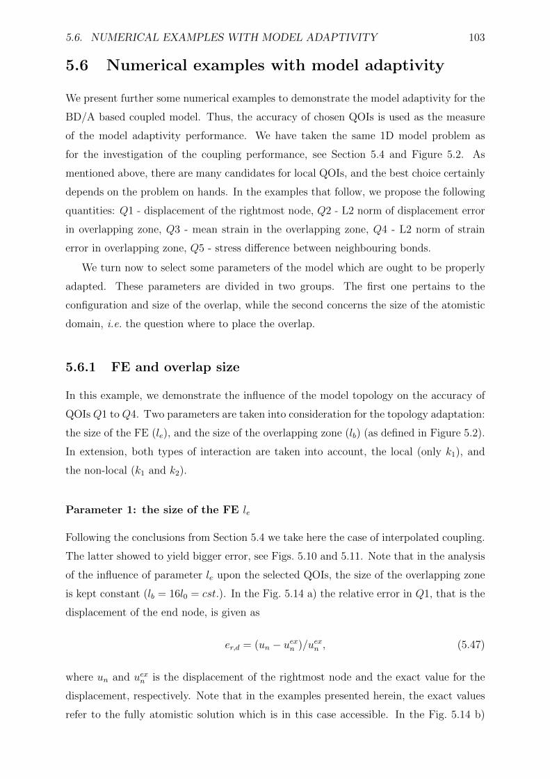
5.6. NUMERICAL EXAMPLES WITH MODEL ADAPTIVITY 103
5.6 Numerical examples with model adaptivity
We present further some numerical examples to demonstrate the model adaptivity for the
BD/A based coupled model. Thus, the accuracy of chosen QOIs is used as the measure
of the model adaptivity performance. We have taken the same 1D model problem as
for the investigation of the coupling performance, see Section 5.4 and Figure 5.2. As
mentioned above, there are many candidates for local QOIs, and the best choice certainly
depends on the problem on hands. In the examples that follow, we propose the following
quantities: Q1 - displacement of the rightmost node, Q2 - L2 norm of displacement error
in overlapping zone, Q3 - mean strain in the overlapping zone, Q4 - L2 norm of strain
error in overlapping zone, Q5 - stress difference between neighbouring bonds.
We turn now to select some parameters of the model which are ought to be properly
adapted. These parameters are divided in two groups. The first one pertains to the
configuration and size of the overlap, while the second concerns the size of the atomistic
domain, i.e. the question where to place the overlap.
5.6.1 FE and overlap size
In this example, we demonstrate the influence of the model topology on the accuracy of
QOIs Q1 to Q4. Two parameters are taken into consideration for the topology adaptation:
the size of the FE (le), and the size of the overlapping zone (lb) (as defined in Figure 5.2).
In extension, both types of interaction are taken into account, the local (only k1), and
the non-local (k1 and k2).
Parameter 1: the size of the FE le
Following the conclusions from Section 5.4 we take here the case of interpolated coupling.
The latter showed to yield bigger error, see Figs. 5.10 and 5.11. Note that in the analysis
of the influence of parameter le upon the selected QOIs, the size of the overlapping zone
is kept constant (lb = 16l0 = cst.). In the Fig. 5.14 a) the relative error in Q1, that is the
displacement of the end node, is given as
er,d = (un − uexn )/uexn , (5.47)
where un and uexn is the displacement of the rightmost node and the exact value for the
displacement, respectively. Note that in the examples presented herein, the exact values
refer to the fully atomistic solution which is in this case accessible. In the Fig. 5.14 b)
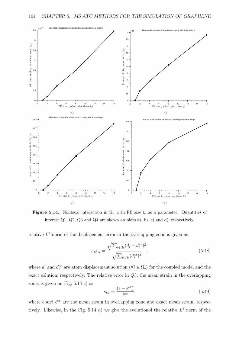
104 CHAPTER 5. MS ATC METHODS FOR THE SIMULATION OF GRAPHENE
0 2 4 6 8 10 12 14 16
0
0.5
1
1.5
2
2.5
3
3.5x 10
−4
FE size le (elem. size times l0)
rel.
errorin
disp.of
theendnod
e,er,d
Non−local interaction, interpolated coupling with linear weight
a)
0 2 4 6 8 10 12 14 16
0
0.5
1
1.5
2
2.5
3
3.5
4
4.5
5x 10
−3
FE size le (elem. size times l0)
L2norm
ofdisp.errorin
Ωb,eL2,d
Non−local interaction, interpolated coupling with linear weight
b)
0 2 4 6 8 10 12 14 16
0
0.01
0.02
0.03
0.04
0.05
0.06
0.07
0.08
FE size le (elem. size times l0)
relativeerrorof
meanstrain
inΩ
b,er,ε
Non−local interaction, interpolated coupling with linear weight
c)
0 2 4 6 8 10 12 14 16
0
0.05
0.1
0.15
0.2
0.25
0.3
0.35
FE size le (elem. size times l0)
L2norm
ofstrain
errorin
Ωb,eL2,ε
Non−local interaction, interpolated coupling with linear weight
d)
Figure 5.14. Nonlocal interaction in Ωa with FE size le as a parameter. Quantities of
interest Q1, Q2, Q3 and Q4 are shown on plots a), b), c) and d), respectively.
relative L2 norm of the displacement error in the overlapping zone is given as
eL2,d =
√∑i∈Ωb
(di − dexi )2√∑i∈Ωb
(dexi )2, (5.48)
where di and dexi are atom displacement solution (∀i ∈ Ωb) for the coupled model and the
exact solution, respectively. The relative error in Q3, the mean strain in the overlapping
zone, is given on Fig. 5.14 c) as
er,ε =(ε− εex)εex
, (5.49)
where ε and εex are the mean strain in overlapping zone and exact mean strain, respec-
tively. Likewise, in the Fig. 5.14 d) we give the evolutionof the relative L2 norm of the
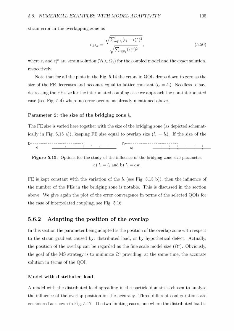
5.6. NUMERICAL EXAMPLES WITH MODEL ADAPTIVITY 105
strain error in the overlapping zone as
eL2,ε =
√∑i∈Ωb
(εi − εexi )2√∑i∈Ωb
(εexi )2, (5.50)
where εi and εexi are strain solution (∀i ∈ Ωb) for the coupled model and the exact solution,
respectively.
Note that for all the plots in the Fig. 5.14 the errors in QOIs drops down to zero as the
size of the FE decreases and becomes equal to lattice constant (le = l0). Needless to say,
decreasing the FE size for the interpolated coupling case we approach the non-interpolated
case (see Fig. 5.4) where no error occurs, as already mentioned above.
Parameter 2: the size of the bridging zone lb
The FE size is varied here together with the size of the bridging zone (as depicted schemat-
ically in Fig. 5.15 a)), keeping FE size equal to overlap size (le = lb). If the size of the
Figure 5.15. Options for the study of the influence of the bridging zone size parameter.
a) le = lb and b) le = cst.
FE is kept constant with the variation of the lb (see Fig. 5.15 b)), then the influence of
the number of the FEs in the bridging zone is notable. This is discussed in the section
above. We give again the plot of the error convergence in terms of the selected QOIs for
the case of interpolated coupling, see Fig. 5.16.
5.6.2 Adapting the position of the overlap
In this section the parameter being adapted is the position of the overlap zone with respect
to the strain gradient caused by: distributed load, or by hypothetical defect. Actually,
the position of the overlap can be regarded as the fine scale model size (Ωa). Obviously,
the goal of the MS strategy is to minimize Ωa providing, at the same time, the accurate
solution in terms of the QOI.
Model with distributed load
A model with the distributed load spreading in the particle domain is chosen to analyse
the influence of the overlap position on the accuracy. Three different configurations are
considered as shown in Fig. 5.17. The two limiting cases, one where the distributed load is
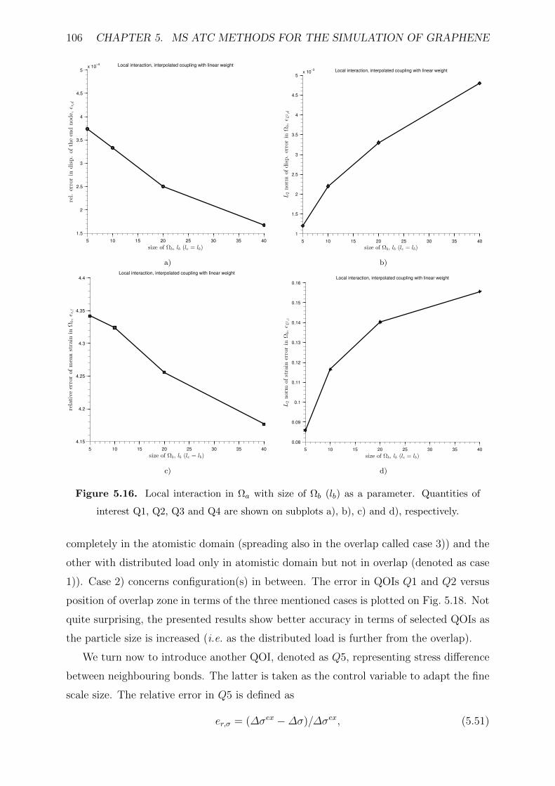
106 CHAPTER 5. MS ATC METHODS FOR THE SIMULATION OF GRAPHENE
5 10 15 20 25 30 35 40
1.5
2
2.5
3
3.5
4
4.5
5x 10
−4
size of Ωb, lb (le = lb)
rel.
errorin
disp.of
theendnod
e,er,d
Local interaction, interpolated coupling with linear weight
a)
5 10 15 20 25 30 35 40
1
1.5
2
2.5
3
3.5
4
4.5
5x 10
−3
size of Ωb, lb (le = lb)
L2norm
ofdisp.errorin
Ωb,eL2,d
Local interaction, interpolated coupling with linear weight
b)
5 10 15 20 25 30 35 40
4.15
4.2
4.25
4.3
4.35
4.4
size of Ωb, lb (le = lb)
relativeerrorof
meanstrain
inΩ
b,er,ε
Local interaction, interpolated coupling with linear weight
c)
5 10 15 20 25 30 35 40
0.08
0.09
0.1
0.11
0.12
0.13
0.14
0.15
0.16
size of Ωb, lb (le = lb)
L2norm
ofstrain
errorin
Ωb,eL2,ε
Local interaction, interpolated coupling with linear weight
d)
Figure 5.16. Local interaction in Ωa with size of Ωb (lb) as a parameter. Quantities of
interest Q1, Q2, Q3 and Q4 are shown on subplots a), b), c) and d), respectively.
completely in the atomistic domain (spreading also in the overlap called case 3)) and the
other with distributed load only in atomistic domain but not in overlap (denoted as case
1)). Case 2) concerns configuration(s) in between. The error in QOIs Q1 and Q2 versus
position of overlap zone in terms of the three mentioned cases is plotted on Fig. 5.18. Not
quite surprising, the presented results show better accuracy in terms of selected QOIs as
the particle size is increased (i.e. as the distributed load is further from the overlap).
We turn now to introduce another QOI, denoted as Q5, representing stress difference
between neighbouring bonds. The latter is taken as the control variable to adapt the fine
scale size. The relative error in Q5 is defined as
er,σ = (∆σex −∆σ)/∆σex, (5.51)
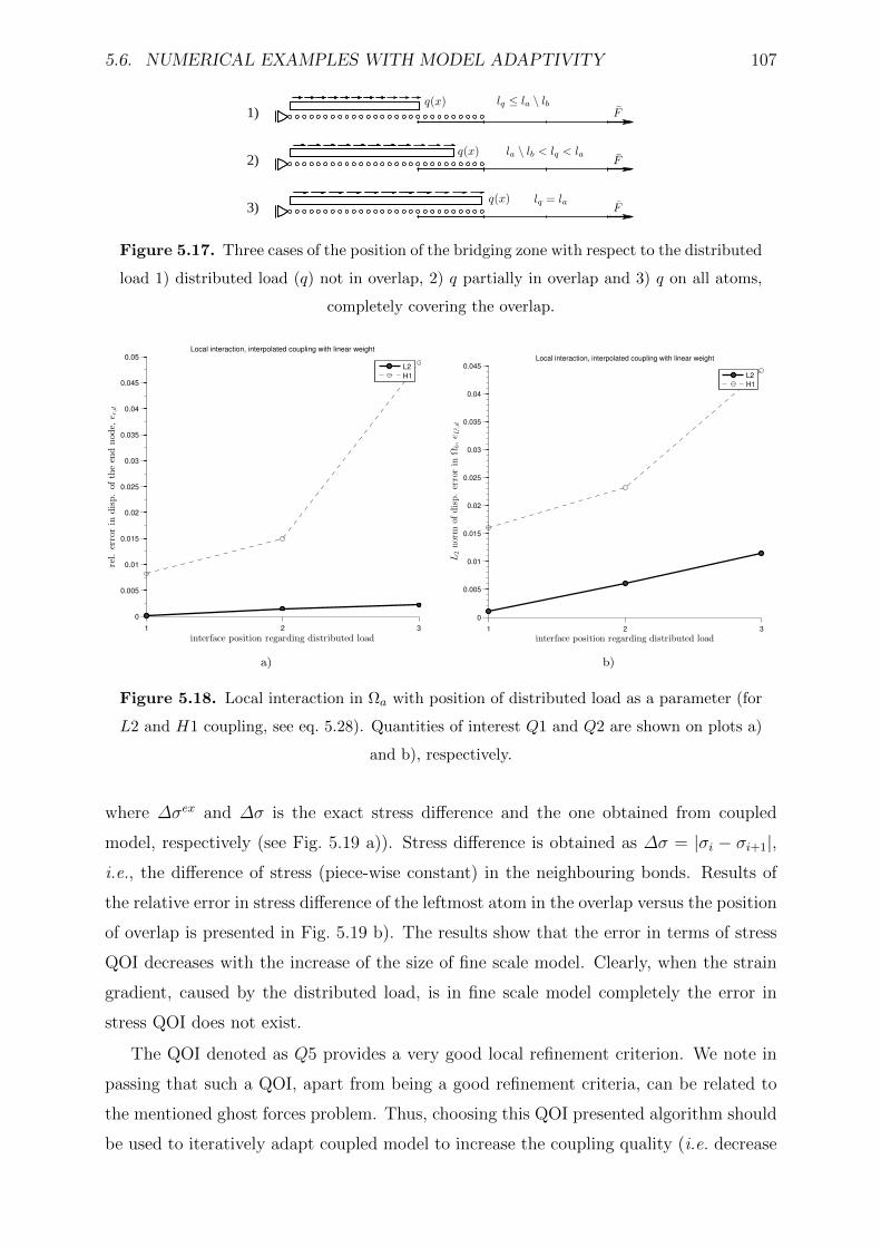
5.6. NUMERICAL EXAMPLES WITH MODEL ADAPTIVITY 107
1)
2)
3)
Figure 5.17. Three cases of the position of the bridging zone with respect to the distributed
load 1) distributed load (q) not in overlap, 2) q partially in overlap and 3) q on all atoms,
completely covering the overlap.
1 2 3
0
0.005
0.01
0.015
0.02
0.025
0.03
0.035
0.04
0.045
0.05
interface position regarding distributed load
rel.
errorin
disp.oftheendnode,
er,d
Local interaction, interpolated coupling with linear weight
L2
H1
a)
1 2 3
0
0.005
0.01
0.015
0.02
0.025
0.03
0.035
0.04
0.045
interface position regarding distributed load
L2norm
ofdisp.errorin
Ωb,eL2,d
Local interaction, interpolated coupling with linear weight
L2
H1
b)
Figure 5.18. Local interaction in Ωa with position of distributed load as a parameter (for
L2 and H1 coupling, see eq. 5.28). Quantities of interest Q1 and Q2 are shown on plots a)
and b), respectively.
where ∆σex and ∆σ is the exact stress difference and the one obtained from coupled
model, respectively (see Fig. 5.19 a)). Stress difference is obtained as ∆σ = |σi − σi+1|,i.e., the difference of stress (piece-wise constant) in the neighbouring bonds. Results of
the relative error in stress difference of the leftmost atom in the overlap versus the position
of overlap is presented in Fig. 5.19 b). The results show that the error in terms of stress
QOI decreases with the increase of the size of fine scale model. Clearly, when the strain
gradient, caused by the distributed load, is in fine scale model completely the error in
stress QOI does not exist.
The QOI denoted as Q5 provides a very good local refinement criterion. We note in
passing that such a QOI, apart from being a good refinement criteria, can be related to
the mentioned ghost forces problem. Thus, choosing this QOI presented algorithm should
be used to iteratively adapt coupled model to increase the coupling quality (i.e. decrease
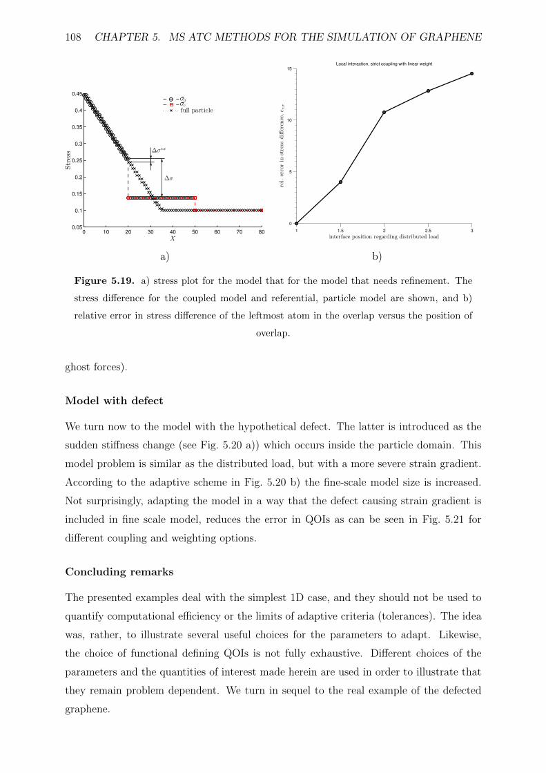
108 CHAPTER 5. MS ATC METHODS FOR THE SIMULATION OF GRAPHENE
a)
1 1.5 2 2.5 3
0
5
10
15
interface position regarding distributed load
rel.
errorin
stress
difference,er,σ
Local interaction, strict coupling with linear weight
b)
Figure 5.19. a) stress plot for the model that for the model that needs refinement. The
stress difference for the coupled model and referential, particle model are shown, and b)
relative error in stress difference of the leftmost atom in the overlap versus the position of
overlap.
ghost forces).
Model with defect
We turn now to the model with the hypothetical defect. The latter is introduced as the
sudden stiffness change (see Fig. 5.20 a)) which occurs inside the particle domain. This
model problem is similar as the distributed load, but with a more severe strain gradient.
According to the adaptive scheme in Fig. 5.20 b) the fine-scale model size is increased.
Not surprisingly, adapting the model in a way that the defect causing strain gradient is
included in fine scale model, reduces the error in QOIs as can be seen in Fig. 5.21 for
different coupling and weighting options.
Concluding remarks
The presented examples deal with the simplest 1D case, and they should not be used to
quantify computational efficiency or the limits of adaptive criteria (tolerances). The idea
was, rather, to illustrate several useful choices for the parameters to adapt. Likewise,
the choice of functional defining QOIs is not fully exhaustive. Different choices of the
parameters and the quantities of interest made herein are used in order to illustrate that
they remain problem dependent. We turn in sequel to the real example of the defected
graphene.
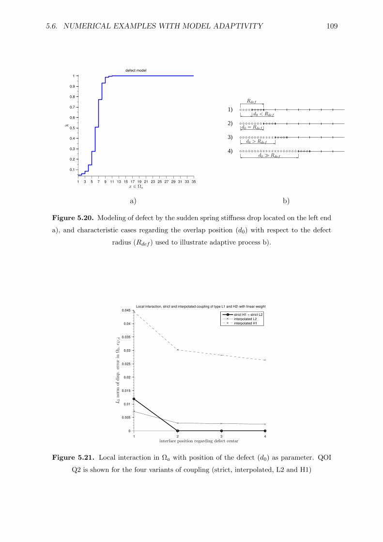
5.6. NUMERICAL EXAMPLES WITH MODEL ADAPTIVITY 109
1 3 5 7 9 11 13 15 17 19 21 23 25 27 29 31 33 35
0.1
0.2
0.3
0.4
0.5
0.6
0.7
0.8
0.9
1
x ∈ Ωa
k
defect model
a)
1)
2)
3)
4)
b)
Figure 5.20. Modeling of defect by the sudden spring stiffness drop located on the left end
a), and characteristic cases regarding the overlap position (d0) with respect to the defect
radius (Rdef ) used to illustrate adaptive process b).
1 2 3 4
0
0.005
0.01
0.015
0.02
0.025
0.03
0.035
0.04
0.045
interface position regarding defect centar
L2norm
ofdisp.errorin
Ωb,eL2,d
Local interaction, strict and interpolated coupling of type L1 and H2\ with linear weight
strict H1 = strict L2
interpolated L2
interpolated H1
Figure 5.21. Local interaction in Ωa with position of the defect (d0) as parameter. QOI
Q2 is shown for the four variants of coupling (strict, interpolated, L2 and H1)
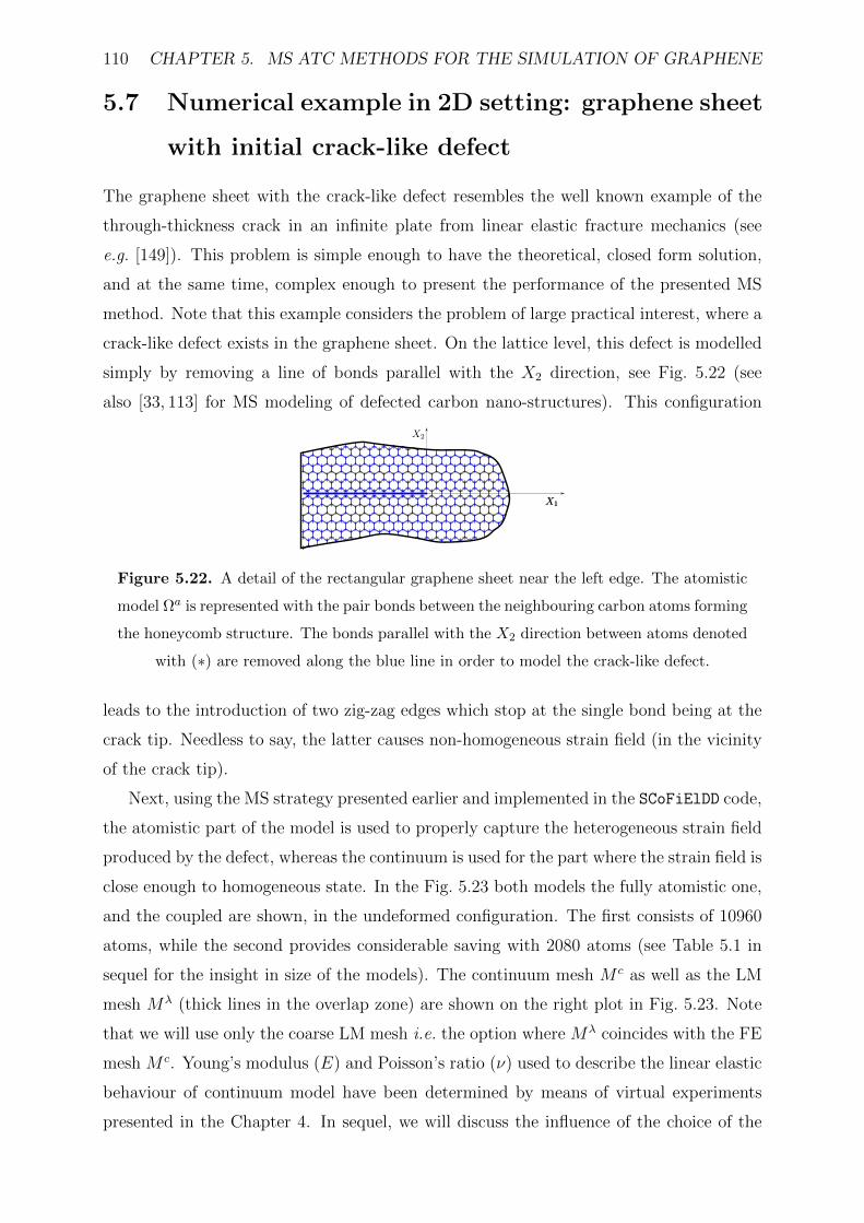
110 CHAPTER 5. MS ATC METHODS FOR THE SIMULATION OF GRAPHENE
5.7 Numerical example in 2D setting: graphene sheet
with initial crack-like defect
The graphene sheet with the crack-like defect resembles the well known example of the
through-thickness crack in an infinite plate from linear elastic fracture mechanics (see
e.g. [149]). This problem is simple enough to have the theoretical, closed form solution,
and at the same time, complex enough to present the performance of the presented MS
method. Note that this example considers the problem of large practical interest, where a
crack-like defect exists in the graphene sheet. On the lattice level, this defect is modelled
simply by removing a line of bonds parallel with the X2 direction, see Fig. 5.22 (see
also [33, 113] for MS modeling of defected carbon nano-structures). This configuration
Figure 5.22. A detail of the rectangular graphene sheet near the left edge. The atomistic
model Ωa is represented with the pair bonds between the neighbouring carbon atoms forming
the honeycomb structure. The bonds parallel with the X2 direction between atoms denoted
with (∗) are removed along the blue line in order to model the crack-like defect.
leads to the introduction of two zig-zag edges which stop at the single bond being at the
crack tip. Needless to say, the latter causes non-homogeneous strain field (in the vicinity
of the crack tip).
Next, using the MS strategy presented earlier and implemented in the SCoFiElDD code,
the atomistic part of the model is used to properly capture the heterogeneous strain field
produced by the defect, whereas the continuum is used for the part where the strain field is
close enough to homogeneous state. In the Fig. 5.23 both models the fully atomistic one,
and the coupled are shown, in the undeformed configuration. The first consists of 10960
atoms, while the second provides considerable saving with 2080 atoms (see Table 5.1 in
sequel for the insight in size of the models). The continuum mesh M c as well as the LM
mesh Mλ (thick lines in the overlap zone) are shown on the right plot in Fig. 5.23. Note
that we will use only the coarse LM mesh i.e. the option where Mλ coincides with the FE
mesh M c. Young’s modulus (E) and Poisson’s ratio (ν) used to describe the linear elastic
behaviour of continuum model have been determined by means of virtual experiments
presented in the Chapter 4. In sequel, we will discuss the influence of the choice of the
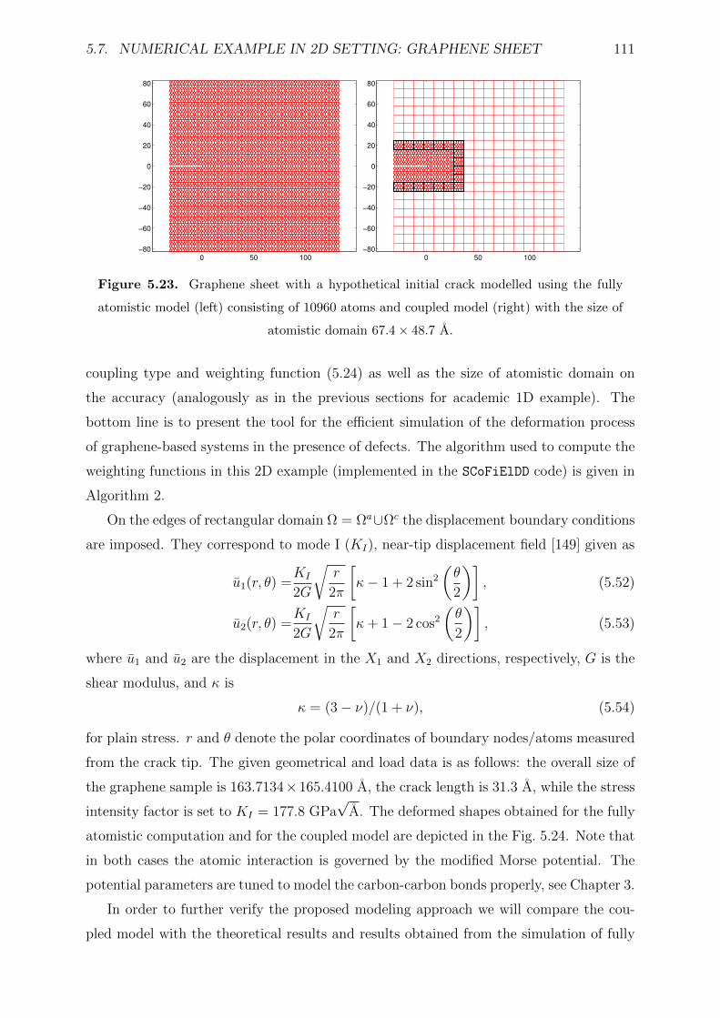
5.7. NUMERICAL EXAMPLE IN 2D SETTING: GRAPHENE SHEET 111
0 50 100
−80
−60
−40
−20
0
20
40
60
80
0 50 100
−80
−60
−40
−20
0
20
40
60
80
Figure 5.23. Graphene sheet with a hypothetical initial crack modelled using the fully
atomistic model (left) consisting of 10960 atoms and coupled model (right) with the size of
atomistic domain 67.4× 48.7 A.
coupling type and weighting function (5.24) as well as the size of atomistic domain on
the accuracy (analogously as in the previous sections for academic 1D example). The
bottom line is to present the tool for the efficient simulation of the deformation process
of graphene-based systems in the presence of defects. The algorithm used to compute the
weighting functions in this 2D example (implemented in the SCoFiElDD code) is given in
Algorithm 2.
On the edges of rectangular domain Ω = Ωa∪Ωc the displacement boundary conditions
are imposed. They correspond to mode I (KI), near-tip displacement field [149] given as
u1(r, θ) =KI
2G
√r
2π
[κ− 1 + 2 sin2
(θ
2
)], (5.52)
u2(r, θ) =KI
2G
√r
2π
[κ+ 1− 2 cos2
(θ
2
)], (5.53)
where u1 and u2 are the displacement in the X1 and X2 directions, respectively, G is the
shear modulus, and κ is
κ = (3− ν)/(1 + ν), (5.54)
for plain stress. r and θ denote the polar coordinates of boundary nodes/atoms measured
from the crack tip. The given geometrical and load data is as follows: the overall size of
the graphene sample is 163.7134×165.4100 A, the crack length is 31.3 A, while the stress
intensity factor is set to KI = 177.8 GPa√
A. The deformed shapes obtained for the fully
atomistic computation and for the coupled model are depicted in the Fig. 5.24. Note that
in both cases the atomic interaction is governed by the modified Morse potential. The
potential parameters are tuned to model the carbon-carbon bonds properly, see Chapter 3.
In order to further verify the proposed modeling approach we will compare the cou-
pled model with the theoretical results and results obtained from the simulation of fully
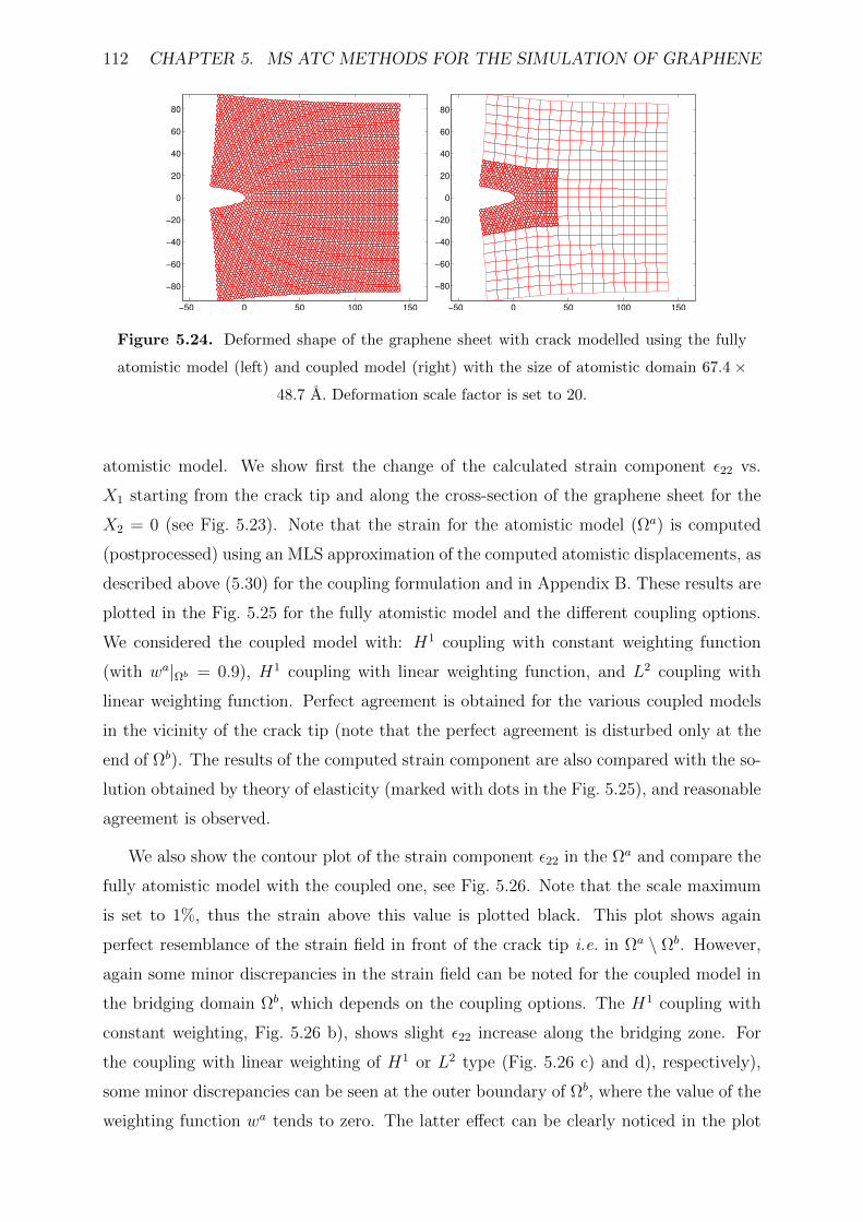
112 CHAPTER 5. MS ATC METHODS FOR THE SIMULATION OF GRAPHENE
−50 0 50 100 150
−80
−60
−40
−20
0
20
40
60
80
−50 0 50 100 150
−80
−60
−40
−20
0
20
40
60
80
Figure 5.24. Deformed shape of the graphene sheet with crack modelled using the fully
atomistic model (left) and coupled model (right) with the size of atomistic domain 67.4 ×48.7 A. Deformation scale factor is set to 20.
atomistic model. We show first the change of the calculated strain component ε22 vs.
X1 starting from the crack tip and along the cross-section of the graphene sheet for the
X2 = 0 (see Fig. 5.23). Note that the strain for the atomistic model (Ωa) is computed
(postprocessed) using an MLS approximation of the computed atomistic displacements, as
described above (5.30) for the coupling formulation and in Appendix B. These results are
plotted in the Fig. 5.25 for the fully atomistic model and the different coupling options.
We considered the coupled model with: H1 coupling with constant weighting function
(with wa|Ωb = 0.9), H1 coupling with linear weighting function, and L2 coupling with
linear weighting function. Perfect agreement is obtained for the various coupled models
in the vicinity of the crack tip (note that the perfect agreement is disturbed only at the
end of Ωb). The results of the computed strain component are also compared with the so-
lution obtained by theory of elasticity (marked with dots in the Fig. 5.25), and reasonable
agreement is observed.
We also show the contour plot of the strain component ε22 in the Ωa and compare the
fully atomistic model with the coupled one, see Fig. 5.26. Note that the scale maximum
is set to 1%, thus the strain above this value is plotted black. This plot shows again
perfect resemblance of the strain field in front of the crack tip i.e. in Ωa \ Ωb. However,
again some minor discrepancies in the strain field can be noted for the coupled model in
the bridging domain Ωb, which depends on the coupling options. The H1 coupling with
constant weighting, Fig. 5.26 b), shows slight ε22 increase along the bridging zone. For
the coupling with linear weighting of H1 or L2 type (Fig. 5.26 c) and d), respectively),
some minor discrepancies can be seen at the outer boundary of Ωb, where the value of the
weighting function wa tends to zero. The latter effect can be clearly noticed in the plot
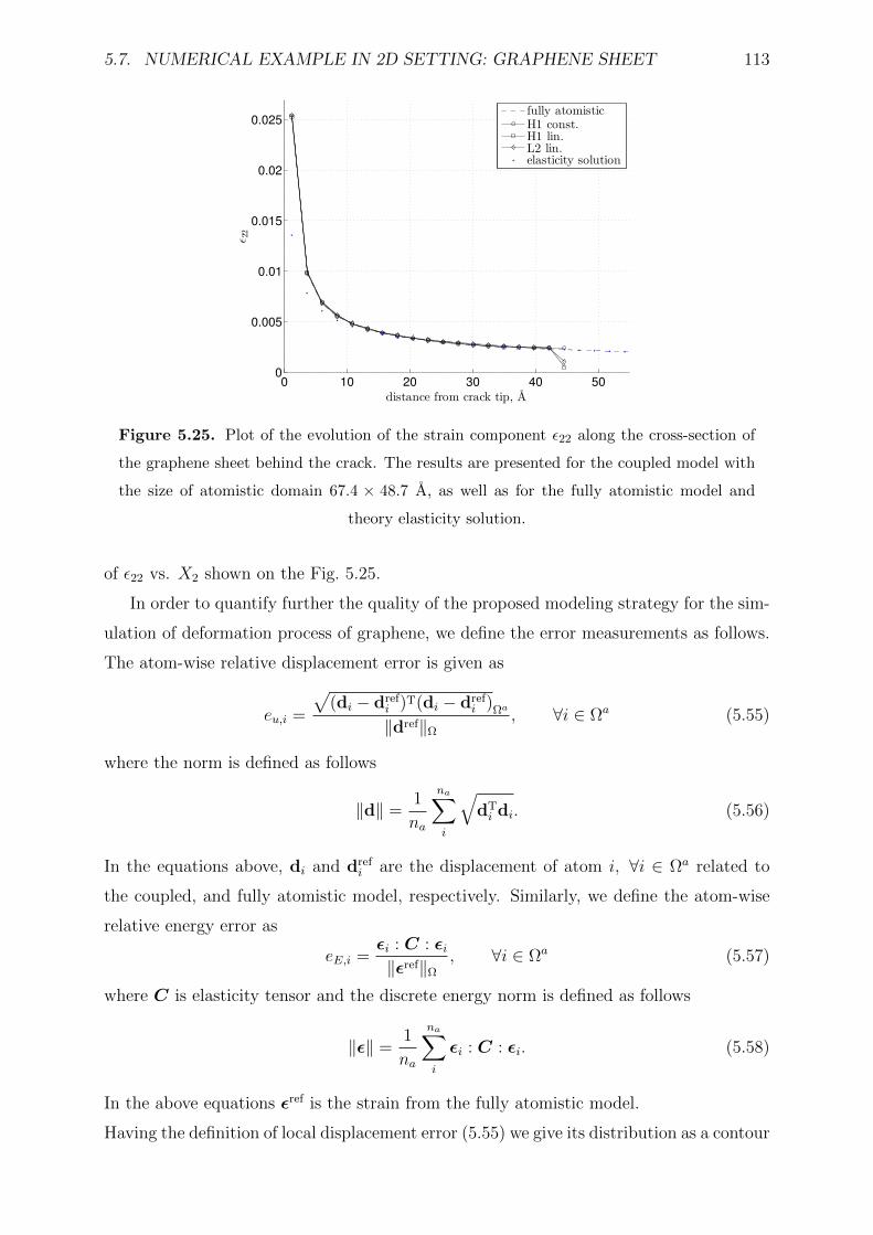
5.7. NUMERICAL EXAMPLE IN 2D SETTING: GRAPHENE SHEET 113
0 10 20 30 40 500
0.005
0.01
0.015
0.02
0.025
distance from crack tip, A
ǫ22
fully atomisticH1 const.H1 lin.L2 lin.elasticity solution
Figure 5.25. Plot of the evolution of the strain component ε22 along the cross-section of
the graphene sheet behind the crack. The results are presented for the coupled model with
the size of atomistic domain 67.4 × 48.7 A, as well as for the fully atomistic model and
theory elasticity solution.
of ε22 vs. X2 shown on the Fig. 5.25.
In order to quantify further the quality of the proposed modeling strategy for the sim-
ulation of deformation process of graphene, we define the error measurements as follows.
The atom-wise relative displacement error is given as
eu,i =
√(di − dref
i )T(di − drefi )Ωa
‖dref‖Ω
, ∀i ∈ Ωa (5.55)
where the norm is defined as follows
‖d‖ =1
na
na∑i
√dTi di. (5.56)
In the equations above, di and drefi are the displacement of atom i, ∀i ∈ Ωa related to
the coupled, and fully atomistic model, respectively. Similarly, we define the atom-wise
relative energy error as
eE,i =εi : C : εi‖εref‖Ω
, ∀i ∈ Ωa (5.57)
where C is elasticity tensor and the discrete energy norm is defined as follows
‖ε‖ =1
na
na∑i
εi : C : εi. (5.58)
In the above equations εref is the strain from the fully atomistic model.
Having the definition of local displacement error (5.55) we give its distribution as a contour
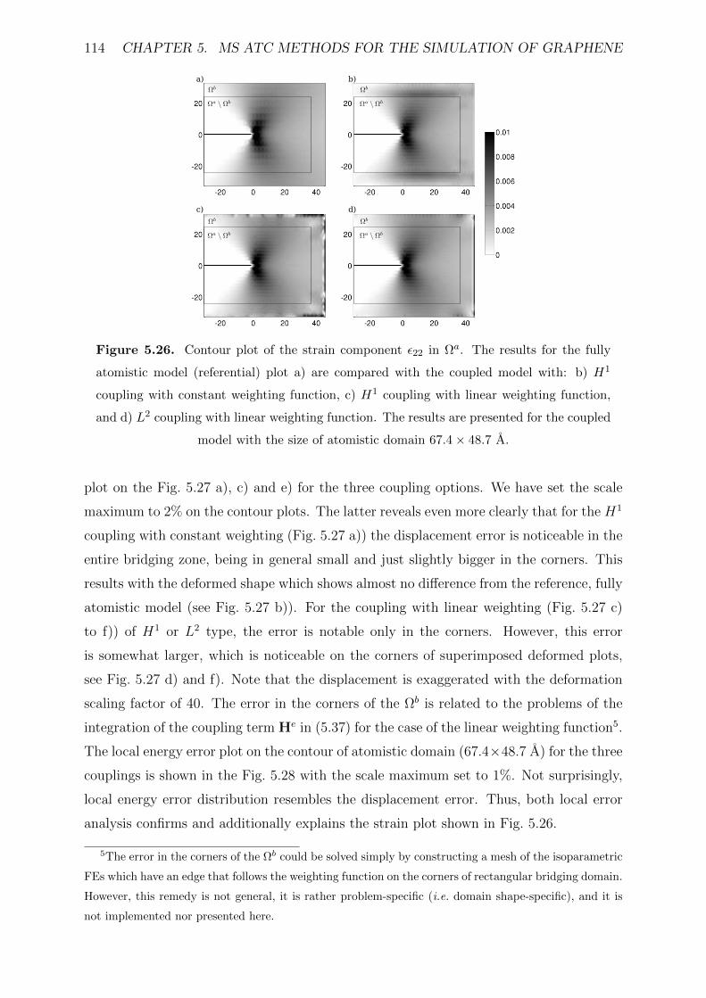
114 CHAPTER 5. MS ATC METHODS FOR THE SIMULATION OF GRAPHENE
a) b)
c) d)
Figure 5.26. Contour plot of the strain component ε22 in Ωa. The results for the fully
atomistic model (referential) plot a) are compared with the coupled model with: b) H1
coupling with constant weighting function, c) H1 coupling with linear weighting function,
and d) L2 coupling with linear weighting function. The results are presented for the coupled
model with the size of atomistic domain 67.4× 48.7 A.
plot on the Fig. 5.27 a), c) and e) for the three coupling options. We have set the scale
maximum to 2% on the contour plots. The latter reveals even more clearly that for the H1
coupling with constant weighting (Fig. 5.27 a)) the displacement error is noticeable in the
entire bridging zone, being in general small and just slightly bigger in the corners. This
results with the deformed shape which shows almost no difference from the reference, fully
atomistic model (see Fig. 5.27 b)). For the coupling with linear weighting (Fig. 5.27 c)
to f)) of H1 or L2 type, the error is notable only in the corners. However, this error
is somewhat larger, which is noticeable on the corners of superimposed deformed plots,
see Fig. 5.27 d) and f). Note that the displacement is exaggerated with the deformation
scaling factor of 40. The error in the corners of the Ωb is related to the problems of the
integration of the coupling term He in (5.37) for the case of the linear weighting function5.
The local energy error plot on the contour of atomistic domain (67.4×48.7 A) for the three
couplings is shown in the Fig. 5.28 with the scale maximum set to 1%. Not surprisingly,
local energy error distribution resembles the displacement error. Thus, both local error
analysis confirms and additionally explains the strain plot shown in Fig. 5.26.
5The error in the corners of the Ωb could be solved simply by constructing a mesh of the isoparametric
FEs which have an edge that follows the weighting function on the corners of rectangular bridging domain.
However, this remedy is not general, it is rather problem-specific (i.e. domain shape-specific), and it is
not implemented nor presented here.
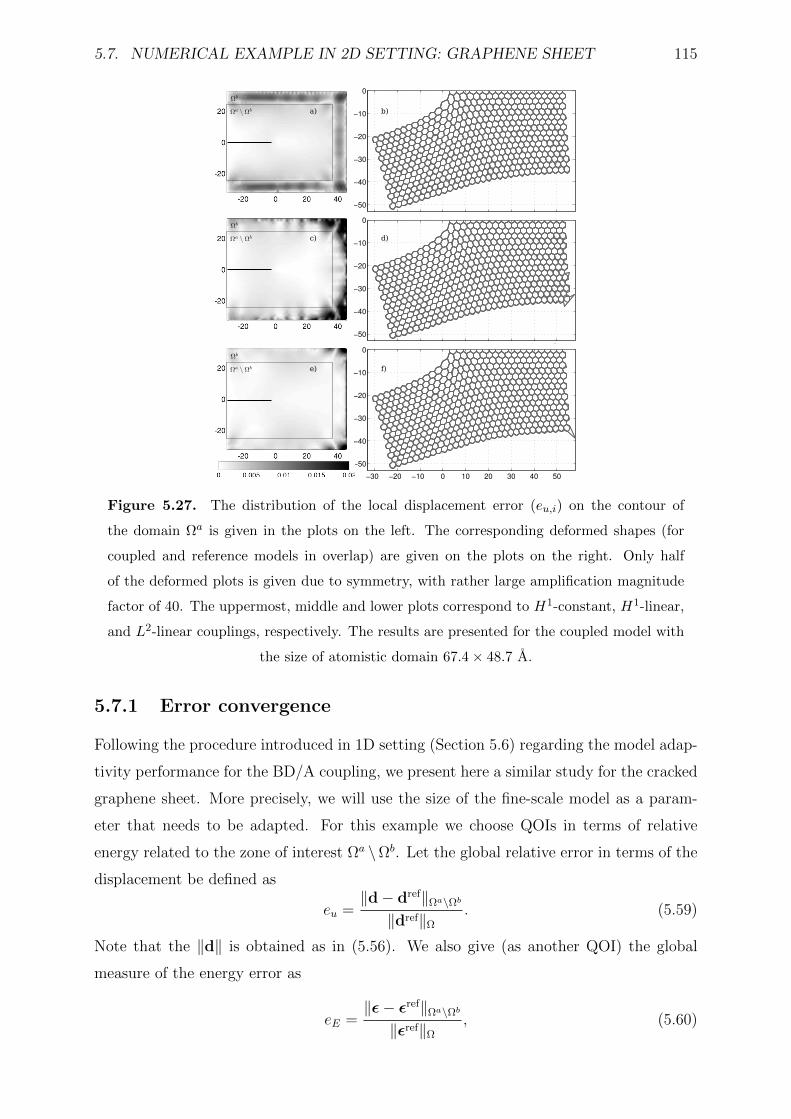
5.7. NUMERICAL EXAMPLE IN 2D SETTING: GRAPHENE SHEET 115
−30 −20 −10 0 10 20 30 40 50
−50
−40
−30
−20
−10
0
−30 −20 −10 0 10 20 30 40 50
−50
−40
−30
−20
−10
0
−30 −20 −10 0 10 20 30 40 50
−50
−40
−30
−20
−10
0
a) b)
c) d)
e) f)
Figure 5.27. The distribution of the local displacement error (eu,i) on the contour of
the domain Ωa is given in the plots on the left. The corresponding deformed shapes (for
coupled and reference models in overlap) are given on the plots on the right. Only half
of the deformed plots is given due to symmetry, with rather large amplification magnitude
factor of 40. The uppermost, middle and lower plots correspond to H1-constant, H1-linear,
and L2-linear couplings, respectively. The results are presented for the coupled model with
the size of atomistic domain 67.4× 48.7 A.
5.7.1 Error convergence
Following the procedure introduced in 1D setting (Section 5.6) regarding the model adap-
tivity performance for the BD/A coupling, we present here a similar study for the cracked
graphene sheet. More precisely, we will use the size of the fine-scale model as a param-
eter that needs to be adapted. For this example we choose QOIs in terms of relative
energy related to the zone of interest Ωa \Ωb. Let the global relative error in terms of the
displacement be defined as
eu =‖d− dref‖Ωa\Ωb
‖dref‖Ω
. (5.59)
Note that the ‖d‖ is obtained as in (5.56). We also give (as another QOI) the global
measure of the energy error as
eE =‖ε− εref‖Ωa\Ωb
‖εref‖Ω
, (5.60)
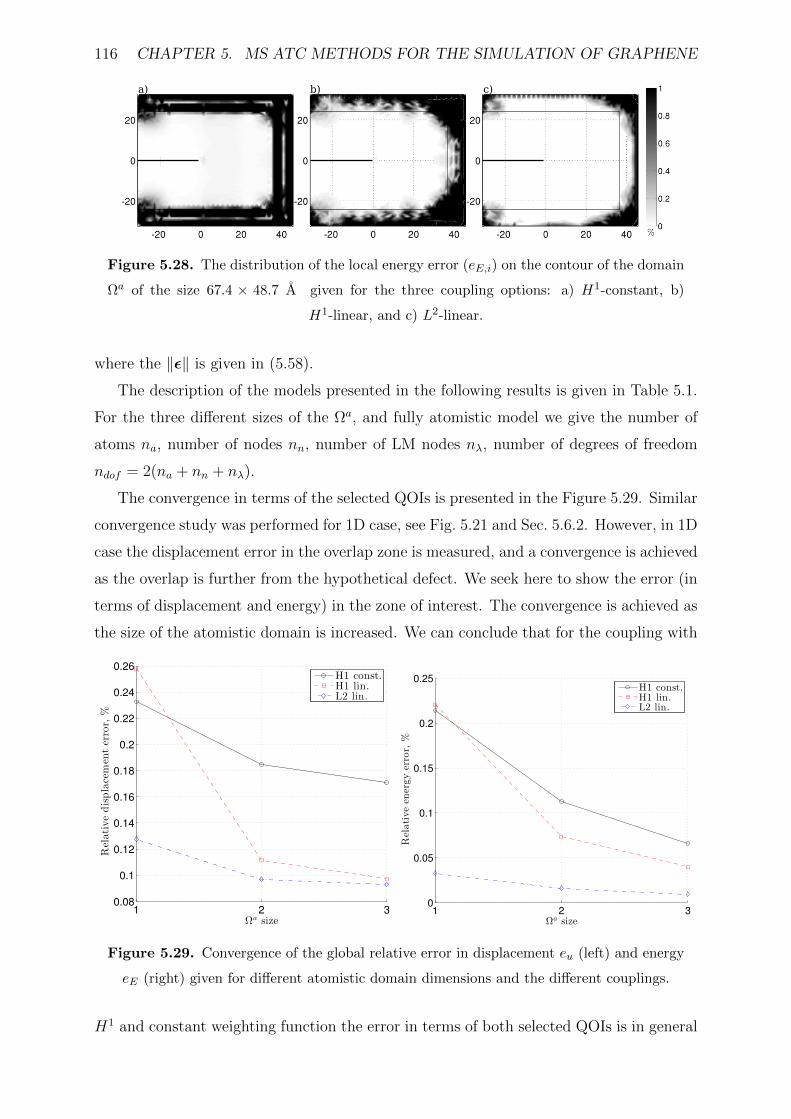
116 CHAPTER 5. MS ATC METHODS FOR THE SIMULATION OF GRAPHENE
a) c)b)
Figure 5.28. The distribution of the local energy error (eE,i) on the contour of the domain
Ωa of the size 67.4 × 48.7 A given for the three coupling options: a) H1-constant, b)
H1-linear, and c) L2-linear.
where the ‖ε‖ is given in (5.58).
The description of the models presented in the following results is given in Table 5.1.
For the three different sizes of the Ωa, and fully atomistic model we give the number of
atoms na, number of nodes nn, number of LM nodes nλ, number of degrees of freedom
ndof = 2(na + nn + nλ).
The convergence in terms of the selected QOIs is presented in the Figure 5.29. Similar
convergence study was performed for 1D case, see Fig. 5.21 and Sec. 5.6.2. However, in 1D
case the displacement error in the overlap zone is measured, and a convergence is achieved
as the overlap is further from the hypothetical defect. We seek here to show the error (in
terms of displacement and energy) in the zone of interest. The convergence is achieved as
the size of the atomistic domain is increased. We can conclude that for the coupling with
1 2 30.08
0.1
0.12
0.14
0.16
0.18
0.2
0.22
0.24
0.26
Ωa size
Relativedisplacemen
terror,
%
H1 const.H1 lin.L2 lin.
1 2 30
0.05
0.1
0.15
0.2
0.25
Ωa size
Relativeen
ergyerror,
%
H1 const.H1 lin.L2 lin.
Figure 5.29. Convergence of the global relative error in displacement eu (left) and energy
eE (right) given for different atomistic domain dimensions and the different couplings.
H1 and constant weighting function the error in terms of both selected QOIs is in general
5.7. NUMERICAL EXAMPLE IN 2D SETTING: GRAPHENE SHEET 117
higher, with the exception of H1-linear. It turns out that the latter yields even higher error
for the smaller sizes of atomistic domain. However, H1-linear coupling decreases rapidly
with the Ωa increase. Note also that for the model denoted as 1 in the Table 5.1 the number
of degrees of freedom is reduced by 84%. Still the corresponding solution yields negligible
error (less then 0.25%) with respect to the fully atomistic model. Thus, both considered
energy scaling constant and linear and coupling types that have been investigated show
really good performance. We would like, however, to point out that for the atomistic-
to-continuum coupling H1 coupling with linear weighting shows no advantage over L2.
Adding the complexity regarding the calculation of the atomistic displacement gradient,
leads to conclusion that for the MS modeling of deformation process of defected graphene
in quasi-static application the L2-linear coupling should be used.
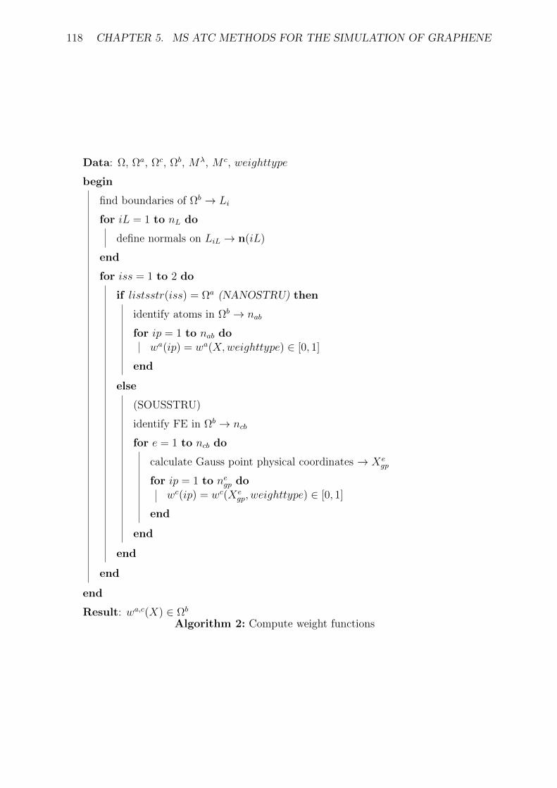
118 CHAPTER 5. MS ATC METHODS FOR THE SIMULATION OF GRAPHENE
Data: Ω, Ωa, Ωc, Ωb, Mλ, M c, weighttype
begin
find boundaries of Ωb → Li
for iL = 1 to nL do
define normals on LiL → n(iL)
end
for iss = 1 to 2 do
if listsstr(iss) = Ωa (NANOSTRU) then
identify atoms in Ωb → nab
for ip = 1 to nab do
wa(ip) = wa(X,weighttype) ∈ [0, 1]
end
else
(SOUSSTRU)
identify FE in Ωb → ncb
for e = 1 to ncb do
calculate Gauss point physical coordinates → Xegp
for ip = 1 to negp do
wc(ip) = wc(Xegp, weighttype) ∈ [0, 1]
end
end
end
end
end
Result: wa,c(X) ∈ Ωb
Algorithm 2: Compute weight functions
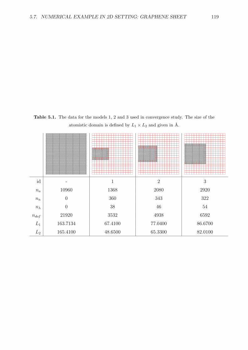
5.7. NUMERICAL EXAMPLE IN 2D SETTING: GRAPHENE SHEET 119
Table 5.1. The data for the models 1, 2 and 3 used in convergence study. The size of the
atomistic domain is defined by L1 × L2 and given in A.
id - 1 2 3
na 10960 1368 2080 2920
nn 0 360 343 322
nλ 0 38 46 54
ndof 21920 3532 4938 6592
L1 163.7134 67.4100 77.0400 86.6700
L2 165.4100 48.6500 65.3300 82.0100

120 CHAPTER 5. MS ATC METHODS FOR THE SIMULATION OF GRAPHENE
Chapter 6Conclusions
In this thesis a new computational methodology capable of predicting the mechanical
behaviour of carbon nano-structures is developed. This methodology at the bottom line
considers the elasto-static simulation of the deformation process of graphene. This chapter
contains an overview of the main results and contributions, as well as the limitations of
the presented formulations and procedures.
In the presented procedures we utilise the atomistic modeling of carbon materials
which is based on the molecular mechanics and classic potentials, namely modified Morse
potential. These models represent nano-scale objects as multiparticle systems considering
every atom in order to properly capture nano-scale phenomena. In particular, each atom
is considered as a classical particle and the atomistic system is treated using Newton’s
laws of mechanics, and not by Schrodinger equation and quantum mechanics. Treating
atoms as classical particles is a significant simplification which has a great impact on the
computability. However, we remark that it represents, also, an important limitation in the
sense of accurate modeling of bond failure and rehybridisation. In addition, we neglected
the dynamic and thermal effects with the assumption of the zero Kelvin temperature.
Considering modified Morse potential, the simulation starts from the equilibrium config-
uration, and we search the new equilibrium for the loaded configuration. The latter is
found by means of full Newton incremental-iterative solver implemented in the in-house
MATLAB code, due to nonlinear nature of the interatomic potential and geometrically non-
linear kinematics. Atomistic internal force vector and tangent stiffness matrix for both
pair and angular term of the modified Morse potential are obtained in closed form and
assembled similarly like in finite element method.
The developed code is further used to compute the equivalent continuum model pa-
rameters through numerical homogenization, i.e., by means of the virtual experiments
on the representative volume element (RVE) of the graphene lattice. The mechanisms
121
122 CHAPTER 6. CONCLUSIONS
responsible for the very wide scatter of reported results on equivalent elastic properties of
graphene are identified. They pertain to formulation differences, choice of the potential,
size effect, relaxation, edge type (chirality and passivation) and definition of the thickness
of the graphene sheet. Moreover, we proved that one of the key factors for the scatter in
Young’s modulus is caused by different types of BC, namely displacement, force or mixed
BC.
The apparent linear elastic stiffness bounds in the homogenisation theory pertain to the
lower bound obtained with homogeneous traction boundary conditions, and the upper
bound obtained with homogeneous displacement boundary conditions. We established
those stiffness bounds in the case of equivalent continuum model of graphene in linear as
well as in nonlinear regime. It has been found that the standard linear stiffness bounds
hold for armchair configuration, while for zigzag configuration they do not. Moreover, for
the non-linear regime with moderate and large strain of the lattice, the stiffness bounds
do not apply.
The development of homogenized constitutive model in large strain regime is based on
the well established continuum mechanics framework (i.e. nonlinear membrane theory),
with the main novelty concerning the specific application to graphene. The benefit of the
familiar continuum mechanics framework is the straightforward finite element implemen-
tation which is relying upon previous works on large deformation of rubber-like materials.
The developed model is fully capable to reproduce the stress release caused by intrinsic
geometric non-linearity of the interatomic bonds that occurs in large strain regime. The
main limitation of the equivalent continuum model of graphene pertains to the inability
to model lattice defects and/or bond fracture.
A convenient solution for this limitation pertains to the MS atomistic-to-continuum
modeling approach. The latter is the elegant way to keep the atomistic model of defected
lattice structure and retain the computational affordability of continuum mechanics in
such a way that atomistic representation is maintained only in the localized region around
defect and is coupled to the equivalent continuum model. There is a number of available
multiscale methods, however we focused on the bridging domain which enables inclusion
of the atomistic submodel or patch (therefore the other name: Arleqin method) in the
continuum model. We showed that the perturbation caused by the coupling of the atom-
istic and continuum models in the overlapping zone is localized. Next, we confronted
bridging domain method with one of the most prominent multiscale methods of this type,
the quasicontinuum method, emphasising the adaptivity features. We implemented model
adaptivity algorithm based on the a posteriori error estimates, and tested its performance
123
on the one-dimensional model by choosing several quantities of interest in terms of dis-
placement, strain and stress. Moreover, we proposed a unified coupling formulation which
shows that the two mentioned mainstream multiscale methods are similar, even though
on the implementation level they may seem completely different. Finally, we extended the
developed algorithm to the real problem of defected graphene sheet. The error analysis,
in terms of displacement and energy, is performed for different weak coupling strategies.
The latter shows an excellent performance of the developed computational methodology.
At the very end it is useful to condense the most important contributions of this
thesis. We emphasized the contribution which are related to 1. the equivalent continuum
modeling as a hierarchical approach to bridge atomistic-to-continuum, 2. the concurrent
atomistic-to-continuum MS modeling, and 3. an overall contribution:
1. Hierarchical MS modeling of graphene
• The main mechanisms resulting in a large dispersion of elastic properties are
identified. Moreover, the influence of the boundary conditions is proved to be
yet another source for the published results discrepancy. The novel elastic stiff-
ness bounds in the equivalent continuum modeling of graphene are developed.
• The development of homogenized hyperelastic constitutive model in terms of
principal stretches for large elastic strain regime. The developed material model
is capable to reproduce the linear elastic behaviour in small strain regime as
well as the stress release caused by intrinsic geometric nonlinearity of the in-
teratomic bonds that occurs in large strain regime.
2. Concurrent MS modeling of graphene
• A unified coupling formulation of the atomistic-to-continuum coupling related
to the two most prominent energy-based, concurrent MS methods is proposed.
• The model adaptivity based on the a posteriori error estimates in certain quan-
tities of interest is implemented in the bridging domain/Arlequin based MS
method, and tested on the number of numerical examples considering graphene.
3. Overall
• An overall contribution is a new computational methodology capable of pre-
dicting the mechanical behaviour of carbon nano-structures, which at the bot-
tom line considers the elasto-static simulation of the deformation process of
graphene.

124 CHAPTER 6. CONCLUSIONS

Appendices
125

Appendix ASolution of system of non-linear algebraic
equations
A.1 Incremental analysis
Before we approach to the incremental analysis let us revisit shortly the method of solution
of the system of linear algebraic equations, which is usually given by
Ku = f ext. (A.1)
This system is solved by well known Gauss method in two phases. First phase concerns
triangular decomposition (which takes most of the computational cost) of system matrix
K into lower triangular L and upper triangular U matrix
K = LU = f ext. (A.2)
Second phase considers forward reduction and back substitution
LUu = Ly = f ext → Ly = f ext (forw. red.)→ Uu = y (back subs.) (A.3)
By using the FEM for solving a boundary value problem considering even a simple
case of non-linear elasticity we obtain a system of non-linear algebraic equations, usually
given by
f int(u) = f ext, (A.4)
where f int and f ext are internal and external force vectors, respectively. This system
is solved incrementally for the displacement values as unknowns. In general, it is not
possible to obtain a closed form solution to a system of nonlinear algebraic equations. For
that reason, we seek an approximate solution by using incremental analysis. The idea is
127
128 APPENDIX A. SOLUTION OF SYSTEM OF NON-LINEAR EQUATIONS
to increase the total load in a sequence of increments which are small enough that the
nonlinear problem under consideration can be approximated by equivalent linear problem.
For the purpose of incremental analysis pseudo-parameter t is usually introduced which
enables eq. A.4 to be rewritten as
f int(u(t)) = f ext(t), t ∈ [0, T ] (A.5)
The given load program is handled through the increments of pseudo-time
[0, T ] =
ninc⋃n=1
[tn, tn+1], (A.6)
where f ext(T ) is the final value of external loading. In the case of proportional loading i.e.
when all the external load components are increasing in the same manner the external
force vector is given as
f ext(t) = f ext0 g(t), (A.7)
where f ext0 is fixed vector and g(t) is a positive increasing function e.g. ramp functiong(t) =
t. The external load increment is given as
∆f extn+1 = f extn+1 − f extn ; f extn+1 = f ext0 g(tn+1), f extn = f ext0 g(tn). (A.8)
The goal is to calculate the value of displacement increment un+1 = ∆dn+1. Using a
consistent linearisation procedure we construct the equivalent linear representation of
given nonlinear problem1. A system of linear algebraic equations is solved by Gauss
method (see A.1)
Knun+1 = ∆f extn+1 (A.9)
to find un+1 and update the displacement vector dn+1 = dn + un+1. This procedure is
schematically depicted in Fig. A.1. Note that we can never have the exact solution to a
nonlinear problem with incremental analysis, even though the solution can be improved
by decreasing the (pseudo-) time steps.
A.2 Newton’s iterative algorithm
Suppose that at time tn the equilibrium equations are satisfied, which can formally be
noted as f int(un) = f extn . At time tn+1 external loading is given by f extn+1 = f extn + ∆f extn+1.
1See [10] p. 57 for more detail explanation of using a directional i.e. Gateaux derivative of scalar
function for constructing consistent linearisation of weak form of a boundary value problem and the
proof of Taylor’s theorem which claims that the tangent stiffness matrix Kn obtain this way presents the
best local approximation of particular nonlinear problem.
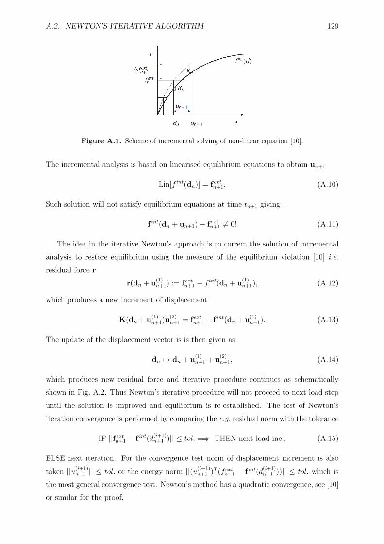
A.2. NEWTON’S ITERATIVE ALGORITHM 129
Figure A.1. Scheme of incremental solving of non-linear equation [10].
The incremental analysis is based on linearised equilibrium equations to obtain un+1
Lin[f int(dn)] = f extn+1. (A.10)
Such solution will not satisfy equilibrium equations at time tn+1 giving
f int(dn + un+1)− f extn+1 6= 0! (A.11)
The idea in the iterative Newton’s approach is to correct the solution of incremental
analysis to restore equilibrium using the measure of the equilibrium violation [10] i.e.
residual force r
r(dn + u(1)n+1) := f extn+1 − f int(dn + u
(1)n+1), (A.12)
which produces a new increment of displacement
K(dn + u(1)n+1)u
(2)n+1 = f extn+1 − f int(dn + u
(1)n+1). (A.13)
The update of the displacement vector is is then given as
dn 7→ dn + u(1)n+1 + u
(2)n+1, (A.14)
which produces new residual force and iterative procedure continues as schematically
shown in Fig. A.2. Thus Newton’s iterative procedure will not proceed to next load step
until the solution is improved and equilibrium is re-established. The test of Newton’s
iteration convergence is performed by comparing the e.g. residual norm with the tolerance
IF ||f extn+1 − f int(d(i+1)n+1 )|| ≤ tol. =⇒ THEN next load inc., (A.15)
ELSE next iteration. For the convergence test norm of displacement increment is also
taken ||u(i+1)n+1 || ≤ tol. or the energy norm ||(u(i+1)
n+1 )T (f extn+1 − f int(d(i+1)n+1 ))|| ≤ tol. which is
the most general convergence test. Newton’s method has a quadratic convergence, see [10]
or similar for the proof.
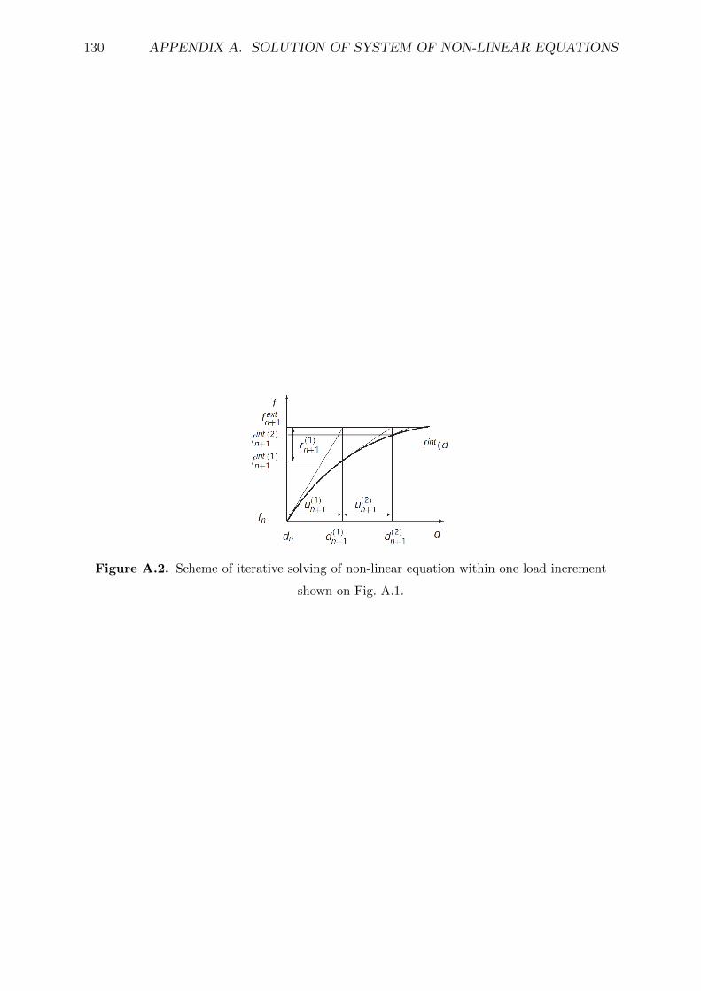
130 APPENDIX A. SOLUTION OF SYSTEM OF NON-LINEAR EQUATIONS
Figure A.2. Scheme of iterative solving of non-linear equation within one load increment
shown on Fig. A.1.
Appendix BMoving least squares approximation
In order to test and to compare the behavior of the L2 and the H1 couplings for continuum
and atomistic models, the intermediate field db(X) is introduced. In this work it is
uniquely defined by an MLS interpolant of the atomistic displacement within the coupling
zone Ωb.
B.1 MLS shape functions
Let the approximation of the displacement in any point X be given as
db(X) :=m∑j=1
pj(X)aj(X) = pT(X)a(X), (B.1)
where m is the number of the terms in the basis p(X), and a(X) is the vector of unknown
coefficients. Note that the coefficients depend on the point X for which the approximated
value is calculated. In this work we used a complete monomial linear basis
pT(X) = [1 X1 X2]. (B.2)
Vector a(X) contains the unknown coefficients
a(X) = [a1(X) a2(X) . . . aj(X) . . . am(X)]T. (B.3)
The values of the unknown coefficients aj(X), ∀j = 1 . . .m, at the point X should be
influenced only by a finite, relatively small number of the nodes, positioned in some
local neighbourhood of X, to keep the computational costs acceptable. The unknown
coefficients can be determined by means of the discrete weighted L2 norm (see e.g. [150–
153])
J =n∑i
w(X−Xi)[pT(Xi)a(X)− di
]→ min, (B.4)
131
132 APPENDIX B. MOVING LEAST SQUARES APPROXIMATION
where di = d(Xi) is the function value at the point Xi, n is the number of points Xi in the
neighbourhood of X (that influence the approximation at that point), and w stands for
the weight function associated with the node X. A fourth-order spline function is chosen
as the weight function
w(r) =
1− 6r2 + 8r3 − 3r4 if r ≤ 1,
0 if r > 1,(B.5)
where r = ‖X − Xi‖/ρ. ρ is the radius that determines the neighbourhood of X and
depends on the atomic lattice constant. Here it is taken to be ρ = 1.8r0.
The minimisation of (B.4), i.e. ∂J∂a
= 0, results in the following linear system
A(X)a(X) = B(X)db. (B.6)
In the above equation A(X) is the moment matrix
A(X) =n∑i
w(X−Xi)p(Xi)pT(Xi), (B.7)
matrix B is given as
B(X) = [B1, . . . ,Bn], Bi = w(X−Xi)p(Xi), (B.8)
and db are the nodal displacement of all the nodes in the neighbourhood of X which can
be written as
db = [d1, . . . , dn]T. (B.9)
Solving (B.3) for a yields
a(X) = A−1(X)B(X)db. (B.10)
Substituting the above equation in (B.1) gives
db(X) := Nmlsdb, (B.11)
where Nmls is the matrix of MLS shape functions.
B.2 MLS interpolant
We turn now to define a continuous interpolant of the atomistic displacement by in-
troducing a relation between the displacement field db(X) and atomistic displacements
di,∀i ∈ Ωa. Due to the lack of Kronecker delta property of the MLS shape functions we
have db(Xi) 6= di. Thus, what we want to enforce is
db(Xi) = di. (B.12)
B.2. MLS INTERPOLANT 133
Taking the above equation and
db(Xi) = Nmls(Xi)db, (B.13)
we can find an invertible matrix D such that
db = Ddb, db = D−1db. (B.14)
The matrix D has the values of the MLS shape functions at the atom positions. Having
this result in hand we can express the displacement interpolation field in terms of the
discrete atomistic displacements (db) as follows
db(X) = Nmls(X)D−1︸ ︷︷ ︸Φ
db, (B.15)
where Φ denotes the interpolant operator. Note that D−1 is a full matrix whose storage
is computationally expensive. However, the MLS interpolation is performed only in the
relatively narrow bridging zone, thus the number of atoms is small and the size being
nba × nba is acceptable.
The described MLS interpolation procedure is implemented in the SCoFiElDD code
presented in the Appendix C.

134 APPENDIX B. MOVING LEAST SQUARES APPROXIMATION
Appendix CComputational code
In this appendix we will present an object oriented MATLAB [154] code named SCoFiElDD
(Structure Computation by Finite Elements and Domain Decomposition). The FE core
of the code was developed in the Laboratory for mechanics and technology (LMT), ENS-
Cachan, France by P.A. Guidault, E. Baranger and G. Lubineau in 2005.
C.1 Code structure
We will first give a Unified Modeling Language (UML) diagram, Fig. C.1. UML is a
pictorial language commonly used to make object oriented software blueprints, thus we
will use it to represent the structure of the SCoFiElDD code. Note that in the Fig. C.1 the
black diamond and white triangle symbols denotes aggregation and heritage, respectively.
The former, often interpreted as has a, denotes that an instance of one class has/contains
an instance of the other class. Heritage (interpreted as is a) means that an instance of
one class belongs to the other class and inherits from its methods. Inheritance is the
mechanism of making new classes from the existing one.
We will give in sequel a brief overview of the classes from the diagram on the Fig. C.1,
which were used in the thesis. Note that the hierarchical level in the lists given below is
reflecting the heritage relations.
Geometrical entities
• STRUCTUR – This class presents the whole model which is composed of at least
one substructure (SOUSSTRU) object
SOUSDOMAI – A subdomain for domain decomposition methods
INTERFACE – An interface for domain decomposition methods
135
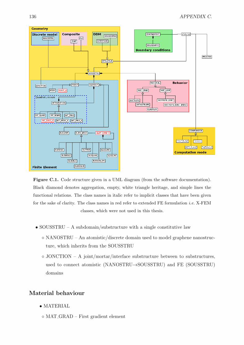
136 APPENDIX C.
Figure C.1. Code structure given in a UML diagram (from the software documentation).
Black diamond denotes aggregation, empty, white triangle heritage, and simple lines the
functional relations. The class names in italic refer to implicit classes that have been given
for the sake of clarity. The class names in red refer to extended FE formulation i.e. X-FEM
classes, which were not used in this thesis.
• SOUSSTRU – A subdomain/substructure with a single constitutive law
NANOSTRU – An atomistic/discrete domain used to model graphene nanostruc-
ture, which inherits from the SOUSSTRU
JONCTION – A joint/mortar/interface substructure between to substructures,
used to connect atomistic (NANOSTRU→SOUSSTRU) and FE (SOUSSTRU)
domains
Material behaviour
• MATERIAL
MAT GRAD – First gradient element
C.1. CODE STRUCTURE 137
ELASTILIN – Elastic model for one-dimensional problems
ISOTROPE – Isotropic material behavior assign to the FE model
Computation mode
• COMPUMODE – Computation mode and problem type, i.e., denomination of the
type of calculation performed (general 3D, plane stress, etc.)
Finite element approximation
• POINT – A geometrical point with local data, which can be a FE node or a
quadrature point
ATOM – An atom for atomistic computation inherits from POINT but have the
neighbouring atom list, and equilibrium distances and angles
• ELEMENT – FE element class
ELEGRAD – First gradient elements
ELEQUA4 – We used quadrilateral isoparametric FE with 4 nodes (many other
FEs like the first order triangular ELETRI3, and second order quadrilateral
ELEQUA8 are implemented in the code)
Quadrature rules
• INTEGRATION – Class used to generate integration objects with the data about
the integration points and weights
INT QUAD – Quadrature for a quadrilateral FE
Boundary conditions
• BOUNDARYC – Contains information considering force and displacement bound-
ary conditions (Lagrange multipliers method is used for the imposition of the bound-
ary conditions)

138 APPENDIX C.
Appendix DZivotopis
Eduard Marenic roden je 29. listopada 1982. u Novskoj. Srednju skolu zavrsio je u
Krizu 2001. godine. Nakon toga, upisao je studij strojarstva na Fakultetu strojarstva i
brodogradnje u Zagrebu, gdje je diplomirao 2007. godine. Od 2008. godine zaposlen je
kao mladi asistent na Zavodu za tehnicku mehaniku na Fakultetu strojarstva i brodograd-
nje u Zagrebu, gdje je pohadao poslijediplomski studij, smjer Teorija konstrukcija. Kao
istrazivac sudjelovao je na tri znanstvena projekta. Tijekom istrazivanja, boravio je tri
mjeseca na Tehnickom Sveucilistu u Darmstadtu, Njemacka, 2010. g. Pocetkom 2012.
godine upisuje dvojni doktorat izmedu Sveucilista u Zagrebu i Ecole Normale Superieure,
Cachan, Francuska, te boravi 18 mjeseci na Ecole Normale Superieure u Cachanu, Fran-
cuska. Uz istrazivacki rad, aktivno je sudjelovao u nastavi iz vise kolegija dodiplomskog
i diplomskog studija. Autor je ukupno 11 znanstvenih radova, od cega je 3 objavljeno u
CC znanstvenim casopisima. Clan je Hrvatskog drustva za mehaniku i Srednje-europskog
udruzenja za racunalnu mehaniku.
139

140 APPENDIX D. ZIVOTOPIS
Appendix EBiography
Eduard Marenic was born on October 29, 1982 in Novska, Croatia. He graduated at the
grammar school in Kriz, Croatia, in 2001. He then enrolled in the graduate study at the
Faculty of Mechanical Engineering and Naval Architecture, University of Zagreb, where
he received the Mag. Ing. Mech. degree in mechanical engineering in 2007. Since 2008,
he has been employed as a junior researcher at the Department of Technical Mechanics
at the Faculty of Mechanical Engineering and Naval Architecture, University of Zagreb,
where he enrolled in the postgraduate study in Theory of Structures and Design. He has
been working as a research assistant on three scientific projects. During his research, he
conducted research at the Department of Civil Engineering and Geodesy, Solid Mechanics
Technical University Darmstadt, Germany, for 3 months in 2010. In 2012 he was enrolled
in the joint PhD program between University of Zagreb and Ecole Normale Superieure,
and conducts research in Cachan for 18 months. In addition, he has been involved in the
teaching activities in a number of courses from the graduate study. He is the first author
of 11 scientific publications, including 3 contributions published in the highly esteemed
CC scientific journals. He is a member of the Croatian Society of Mechanics and the
Central European Association for Computational Mechanics.
141

142 APPENDIX E. BIOGRAPHY
Bibliography
[1] A. Kis and A. Zettl. Nanomechanics of carbon nanotubes. Phil. Trans. R. Soc. A,
366:1591–1611, 2008.
[2] S. Iijima. Helical microtubules of graphitic carbon. Naure, 354:56–58, 1991.
[3] K. S. Novoselov, D. Jiang, F. Schedin, T. J. Booth, V. V. Khotkevich, S. V. Morozov,
and A. K. Geim. Two-dimensional atomic crystals. PNAS, 102-30:1045110453, 2005.
[4] S. Bae, H. Kim, Y. Lee, X. Xu, J.-S. Park, Y. Zheng, J. Balakrishnan, T. Lei,
H. Ri Kim, Y. I. Song, Y.-J. Kim, K. S. Kim, B. Ozyilmaz, J.-H. Ahn, B. H. Hong,
and S. Iijima. Roll-to-roll production of 30-inch graphene films for transparent
electrodes. Nat Nano, 5(8):574–578, 2010.
[5] F. Banhart, J. Kotakoski, and A. V. Krasheninnikov. Structural defects in graphene.
ACSNANO, 5-1:26–41, 2011.
[6] P. T. Araujo, M. Terrones, and M. S. Dresselhaus. Defects and impurities in
graphene-like materials. Materials Today, 15(3):98 – 109, 2012.
[7] J. Lahiri, Y. Lina, P. Bozkurt, I. I. Oleynik, and M. Batzill. An extended defect in
graphene as a metallic wire. Nat Nano, 5:326 – 329, 2005.
[8] M.-F. Yu, O. Lourie, M. J. Dyer, K. Moloni, T. F. Kelly, and R. S. Ruoff. Strength
and breaking mechanism of multiwalled carbon nanotubes under tensile load. Sci-
ence, 287:637–640, 2000.
[9] C. Lee, X. Wei, J. Kysar, and J. Hone. Measurement of the elastic properties and
intrinsic strength of monolayer graphene. Science, 321(5887):385–388, 2008.
[10] A. Ibrahimbegovic. Nonlinear Solid Mechanics. Springer, 2009.
143
144 BIBLIOGRAPHY
[11] P. Wriggers. Nonlinear Finite Element Methods. Springer, 2008.
[12] G. A. Holzapfel. Nonlinear Solid Mechanics: A Continuum Approach For Engineer-
ing. John Wiley, 2000.
[13] M. J. Buehler. Atomistic Modeling of Materials Failure. Springer US, 2008.
[14] D. C. Rapaport. The Art of Molecular Dynmics Simulations. Cambridge University
Press, 2004.
[15] R. Phillips. Crystals, Defects and Microstructures Modeling Across Scales. Cam-
bridge University Press, 2004.
[16] W. K. Liu, E. G. Karpov, and H. S. Park. Nano Mechanics and Materials Theory,
Multiscale Methods and Applications. John Wiley & Sons, Ltd, 2006.
[17] A. N. Cleland. Foundations of Nanomechanics From Solid-State Theory to Device
Applications. Springer, 2003.
[18] M. Griebel, S. Knapek, and G. Zumbusch. Numerical Simulation in Molecular
Dynamics. Springer, Berlin, Heidelberg, 2007.
[19] Lammps www site. http://http://lammps.sandia.gov/index.html, 2013.
[20] S. Plimpton. Fast parallel algorithms for shortrange molecular dynamics. Journal
of Computational Physics, 117:1–19, 1995.
[21] F. Ercolessi. A molecular dynamics primer, June 1997.
[22] E. Sanchez-Palencia. Non-homogeneous media and vibration theory. Springer, 1980.
[23] J. Fish. Multiscale Methods Bridging the Scales in Science and Engineering. Oxford
Univeristy press, 2009.
[24] W. A. Curtin and R. E. Miller. Atomistic/continuum coupling in computational
materials science. Modelling Simul. Mater. Sci. Eng., 11:33–68, 2003.
[25] W. K. L. Harold S. Park. An introduction and tutorial on multiple-scale analysis in
solids. Computer Methods in Applied Mechanics and Engineering, 193:1733–1772,
2004.
[26] W. K. Liu, E. G. Karpov, S. Zhang, and H. S. Park. An introduction to computa-
tional nanomechanics and materials. Computer Methods in Applied Mechanics and
Engineering, 193(17-20):1529 – 1578, 2004.
BIBLIOGRAPHY 145
[27] R. Rudd and J. Broughton. Concurrent coupling of length scales in solid state
systems. physica status solidi (b), 217:251–291, 2000.
[28] R. E. Miller and E. B. Tadmor. A unified framework and performance benchmark
of fourteen multiscale atomistic/continuum coupling methods. Modeling and Sim-
ulation in Materials Science and Engineering, 17:053001, 2009.
[29] J. Q. Broughton, F. F. Abraham, N. Bernstein, and E. Kaxiras. Concurrent coupling
of length scales: Methodology and application. Phys. Rev. B, 60(4):2391–2403, Jul
1999.
[30] D. Srivastava and S. N. Atluri. Computational nanotechnology: A current perspec-
tive. CMES, 3:531–538, 2002.
[31] T. Belytschko and S. P. Xiao. Coupling methods for continuum model with molec-
ular model. International Journal for Multiscale Computational Engineering, 1:12,
2003.
[32] E. B. Tadmor, M. Ortiz, and R. Phillips. Quasicontinuum analysis of defects in
solids. Philosophical Magazine A, 73:1529–1563, 1996.
[33] S. Zhang, R. Khare, Q. Lu, and T. Belytschko. A bridging domain and strain com-
putation method for coupled atomistic-continuum modelling of solids. International
Journal for Multiscale Computational Engineering, 70:913–933, 2007.
[34] P. Guidault and T. Belytschko. Bridging domain methods for coupled atomistic-
continuum models with l2 or h1 couplings. International Journal for Numerical
Methods in Engineering, 77-11:1566–1592, 2009.
[35] H. B. Dhia and G. Rateau. The Arlequin method as a flexible engineering design
tool. International Journal for Numerical Methods in Engineering, 62:1442–1462,
2005.
[36] P. T. Bauman, H. B. Dhia, N. Elkhodja, J. T. Oden, and S. Prudhomme. On
the application of the arlequin method to the coupling of particle and continuum
models. Computational Mechanics, 42:511–530, 2008.
[37] S. Prudhomme, H. B. Dhia, P. Bauman, N. Elkhodja, and J. Oden. Computa-
tional analysis of modeling error for the coupling of particle and continuum models
146 BIBLIOGRAPHY
by the Arlequin method. Computer Methods in Applied Mechanics and Engineer-
ing, 197(41-42):3399 – 3409, 2008. Recent Advances in Computational Study of
Nanostructures.
[38] P. T. Bauman, J. T. Oden, and S. Prudhomme. Adaptive multiscale modeling
of polymeric materials with arlequin coupling and goals algorithms. Computer
Methods in Applied Mechanics and Engineering, 198:799 – 818, 2009.
[39] S. Prudhomme, L. Chamoin, H. B. Dhia, and P. T. Bauman. An adaptive strategy
for the control of modeling error in two-dimensional atomic-to-continuum coupling
simulations. Computer Methods in Applied Mechanics and Engineering, 198(21-
26):1887 – 1901, 2009. Advances in Simulation-Based Engineering Sciences - Hon-
oring J. Tinsley Oden.
[40] T. Shimokawa, J. J. Mortensen, J. Schiøtz, and K. W. Jacobsen. Matching con-
ditions in the quasicontinuum method: Removal of the error introduced at the
interface between the coarse-grained and fully atomistic region. Phys. Rev. B,
69(21):214104, Jun 2004.
[41] L. Chamoin, S. Prudhomme, H. Ben Dhia, and T. Oden. Ghost forces and spu-
rious effects in atomic-to-continuum coupling methods by the arlequin approach.
International Journal for Numerical Methods in Engineering, 83:1081–1113, 2010.
[42] G. Anciaux, O. Coulaud, J. Roman, and G. Zerah. Ghost force reduction and
spectral analysis of the 1d bridging method. Research Report RR-6582, INRIA,
2008.
[43] J. Oden and K. S. Vemaganti. Estimation of local modeling error and goal-oriented
adaptive modeling of heterogeneous materials: I. error estimates and adaptive al-
gorithms. Journal of Computational Physics, 164(1):22 – 47, 2000.
[44] H. B. Dhia, L. Chamoin, J. T. Oden, and S. Prudhomme. A new adaptive modeling
strategy based on optimal control for atomic-to-continuum coupling simulations.
Computer Methods in Applied Mechanics and Engineering, In Press, Corrected
Proof:–, 2010.
[45] M. Ainsworth and J. Oden. A posteriori error estimation in finite element analysis.
Computer Methods in Applied Mechanics and Engineering, 142(12):1 – 88, 1997.
BIBLIOGRAPHY 147
[46] S. Prudhomme, J. T. Oden, T. Westermann, J. Bass, and M. E. Botkin. Practical
methods for a posteriori error estimation in engineering applications. International
Journal for Numerical Methods in Engineering, 56(8):1193–1224, 2003.
[47] J. Oden, S. Prudhomme, and P. Bauman. On the extension of goal-oriented error
estimation and hierarchical modeling to discrete lattice models. Computer Methods
in Applied Mechanics and Engineering, 194(3435):3668 – 3688, 2005.
[48] D. Qian, G. J. Wagner, W. K. Liu, Min-Fen, and Y. Rodney. Mechanics of carbon
nanotubes. Applied Mechanics Reviews, 55:495–553, 2002.
[49] T. Belytschko, S. P. Xiao, G. C. Schatz, and R. S. Ruoff. Atomistic simulations of
nanotube fracture. Phys. Rev. B, 65(23):235430, Jun 2002.
[50] R. S. Ruoff, D. Qian, and W. K. Liu. Mechanical properties of carbon nanotubes:
theoretical predictions and experimental measurements. Comptes Rendus Physique,
4(9):993 – 1008, 2003.
[51] J. Xiao, J. Staniszewski, and J. G. Jr. Fracture and progressive failure of defective
graphene sheets and carbon nanotubes. Composite Structures, 88(4):602 – 609,
2009.
[52] J. Xiao, J. Staniszewski, and J. G. Jr. Tensile behaviors of graphene sheets and car-
bon nanotubes with multiple stonewales defects. Materials Science and Engineering:
A, 527(3):715 – 723, 2010.
[53] P. Atkins and J. De Paula. Physical Chemistry. Oxford University Press, 8rev ed
edition, March 2006.
[54] A. K. Geim and K. S. Novoselov. The rise of graphene. Nature Materials, 6:183–191,
March 2007.
[55] V. Singh, D. Joung, L. Zhai, S. Das, S. I. Khondaker, and S. Seal. Graphene based
materials: Past, present and future. Progress in Materials Science, 56(8):1178 –
1271, 2011.
[56] M. Topsakal and S. Ciraci. Elastic and plastic deformation of graphene, silicene,
and boron nitride honeycomb nanoribbons under uniaxial tension: A first-principles
density-functional theory study. Phys. Rev. B, 81:024107, Jan 2010.
148 BIBLIOGRAPHY
[57] Z. H. Ni, T. Yu, Y. H. Lu, Y. Y. Wang, Y. P. Feng, and Z. X. Shen. Uniaxial
strain on graphene: Raman spectroscopy study and band-gap opening. ACS Nano,
2(11):2301–2305, 2008.
[58] S. Georgantzinos, D. Katsareas, and N. Anifantis. Limit load analysis of graphene
with pinhole defects: A nonlinear structural mechanics approach. International
Journal of Mechanical Sciences, 55(1):85 – 94, 2012.
[59] T. Kuila, S. Bose, P. Khanra, A. K. Mishra, N. H. Kim, and J. H. Lee. Recent
advances in graphene-based biosensors. Biosensors and Bioelectronics, 26:46374648,
2011.
[60] Q. Zhou and A. Zettl. Electrostatic graphene loudspeaker. ArXiv e-prints, March
2013.
[61] K. S. Kim, Y. Zhao, H. Jang, S. Y. Lee, J. M. Kim, K. S. Kim, J.-H. Ahn, P. Kim,
J.-Y. Choi, and B. H. Hong. Large-scale pattern growth of graphene films for
stretchable transparent electrodes. Nature, 457:706 – 710, 2009.
[62] I. W. Frank, D. M. Tanenbaum, A. M. van der Zande, and P. L. McEuen. Mechanical
properties of suspended graphene sheets. Journal of Vacuum Science Technology B:
Microelectronics and Nanometer Structures, 25:2558, 2007.
[63] M. P. Allen and D. J. Tildesley. Computer simulation of liquids. Oxford Univeristy
press, 1987.
[64] D. Keffer. The working person’s guide to molecular dynamics simulations, October
2001.
[65] R. Sunyk. On Aspects of Mixed Continuum-Atomistic Material Modelling. PhD
thesis, Fachbereich Maschinenbau und Verfahrenstechnik der Technischen Universit
at Kaiserslautern, 2004.
[66] S. Georgantzinos, G. Giannopoulos, and N. Anifantis. Numerical investigation
of elastic mechanical properties of graphene structures. Materials & Design,
31(10):4646 – 4654, 2010.
[67] S. Ghosh and M. Arroyo. An atomistic-based foliation model for multilayer graphene
materials and nanotubes. Journal of the Mechanics and Physics of Solids, 61(1):235
– 253, 2013.
BIBLIOGRAPHY 149
[68] P. M. Morse. Diatomic molecules according to the wave mechanics. ii. vibrational
levels. Phys. Rev., 34:57–64, Jul 1929.
[69] M. S. Daw and M. I. Baskes. Embedded-atom method: Derivation and application
to impurities, surfaces, and other defects in metals. Physical Review, 29:6443–6453,
1983.
[70] M. Doyama and Y. Kogure. Embedded atom potentials in fcc and bcc metals.
Computational Materials Science, 14(1-4):80 – 83, 1999.
[71] A. S. Elizondo. Horizontal Coupling in Continuum Atomistics. PhD thesis, Fach-
bereich Maschinenbau und Verfahrenstechnik der Technischen Universitat Kaiser-
slautern, 2007.
[72] F. H. Stillinger and T. A. Weber. Erratum: Computer simulation of local order in
condensed phases of silicon [phys. rev. b 31, 5262 (1985)]. Phys. Rev. B, 33:1451–
1451, Jan 1986.
[73] J. Tersoff. New empirical model for the structural properties of silicon. Phys. Rev.
Lett., 56:632–635, Feb 1986.
[74] D. W. Brenner. Empirical potential for hydrocarbons for use in simulating the
chemical vapor deposition of diamond films. Phys. Rev. B, 42:9458–9471, Nov
1990.
[75] P. Zhang, Y. Huang, P. Geubelle, P. Klein, and K. Hwang. The elastic modulus
of single-wall carbon nanotubes: a continuum analysis incorporating interatomic
potentials. International Journal of Solids and Structures, 39(1314):3893 – 3906,
2002.
[76] D. W. Brenner, O. A. Shenderova, J. A. Harrison, S. J. Stuart, B. Ni, and S. B.
Sinnott. A second-generation reactive empirical bond order (rebo) potential energy
expression for hydrocarbons. Journal of Physics: Condensed Matter, 14(4):783,
2002.
[77] E. Marenic, A. Ibrahimbegovic, J. Soric, and P.-A. Guidault. Homogenized elastic
properties of graphene for small deformations. Materials: Special Issue “Computa-
tional Modeling and Simulation in Materials Study”, 6(9):3764–3782, 2013.
[78] J. Soric. Metoda konacnih elemenata. Golden marketing - Tehnicka knjiga, 2004.
150 BIBLIOGRAPHY
[79] A. Ibrahimbegovic, G. Herve, and P. Villon. Nonlinear impact dynamics and field
transfer suitable for parametric design studies. Engineering Computations, 26:185
– 204, 2009.
[80] B. Liu, Y. Huang, H. Jiang, S. Qu, and K. C. Hwang. The atomic-scale finite ele-
ment method. Computer Methods in Applied Mechanics and Engineering, 193(17-
20):1849 – 1864, 2004.
[81] B. Liu, H. Jiang, Y. Huang, S. Qu, M.-F. Yu, and K. C. Hwang. Atomic-scale finite
element method in multiscale computation with applications to carbon nanotubes.
Phys. Rev. B, 72(3):035435, Jul 2005.
[82] B. Liu, Z. Zhang, and Y. Chen. Atomistic statics approaches - molecular mechanics,
finite element method and continuum. Journal of computational and theoretical
nanoscience, 5:1891–1913, 2008.
[83] Y. Wang, C. Zhang, E. Zhou, C. Sun, J. Hinkley, T. S. Gates, and J. Su. Atom-
istic finite elements applicable to solid polymers. Computational Materials Science,
36(3):292 – 302, 2006.
[84] J. Wackerfuss. Molecular mechanics in the context of the finite element method.
International Journal for Numerical Methods in Engineering, 77:969–997, 2009.
[85] E. Marenic, A. Ibrahimbegovic, and J. Soric. Adaptive modelling in atomistic-to-
continuum multiscale methods. Journal of the Serbian Society for Computational
Mechanics (JSSCM), 6(1):169–198, 2012.
[86] J. L. Ericksen. The cauchy and born hypotheses for crystals. Phase transformation
and material instabilities in solids - from book ’Mechanics and Mathematics of
Crystals: Selected Papers of J. L. Ericksen’ by Millard F. Beatty and Michael A.
Hayes, page 6177, 1984.
[87] J. Ericksen. On the cauchyborn rule. Mathematics and Mechanics of Solids, 13:199–
220, 2008.
[88] S. P. Xiao and T. Belytschko. A bridging domain method for coupling continua with
molecular dynamics. Computer Methods in Applied Mechanics and Engineering,
193(17-20):1645 – 1669, 2004.
BIBLIOGRAPHY 151
[89] A. Ibrahimbegovic and F. Gruttmann. A consistent finite element formulation of
nonlinear membrane shell theory with particular reference to elastic rubberlike ma-
terial. Finite Elements in Analysis and Design, 12:75–86, 1993.
[90] C. D. Reddy, S. Rajendran, and K. M. Liew. Equilibrium configuration and contin-
uum elastic properties of finite sized graphene. Nanotechnology, 17(3):864, 2006.
[91] M. Arroyo and T. Belytschko. Finite crystal elasticity of carbon nanotubes based
on the exponential cauchy-born rule. Phys. Rev. B, 69:115415, Mar 2004.
[92] H. Zhao, K. Min, and N. R. Aluru. Size and chirality dependent elastic properties
of graphene nanoribbons under uniaxial tension. Nanoletters, 9-8:3012–3015, 2009.
[93] G. V. Lier, C. V. Alsenoy, V. V. Doren, and P. Geerlings. Ab initio study of the
elastic properties of single-walled carbon nanotubes and graphene. Chemical Physics
Letters, 326(12):181 – 185, 2000.
[94] K. N. Kudin, G. E. Scuseria, and B. I. Yakobson. c2F, bn, and c nanoshell elasticity
from ab initio computations. Phys. Rev. B, 64:235406, Nov 2001.
[95] Z. Xu. Graphene nano-ribbons under tension. Journal of Computational and The-
oretical Nanoscience, 6:625–628, 2009.
[96] Q. Lu and R. Huang. Excess energy and deformation along free edges of graphene
nanoribbons. Phys. Rev. B, 81:155410, Apr 2010.
[97] Q. Lu, W. Gao, and R. Huang. Atomistic simulation and continuum modeling of
graphene nanoribbons under uniaxial tension. Modelling and Simulation in Mate-
rials Science and Engineering, 19(5):054006, 2011.
[98] G. M. Odegard, T. S. Gates, L. M. Nicholson, and K. E. Wise. Equivalent-
continuum modeling of nano-structured materials. Composites Science and Tech-
nology, 62(14):1869 – 1880, 2002.
[99] F. Scarpa, S. Adhikari, and A. S. Phani. Effective elastic mechanical properties of
single layer graphene sheets. Nanotechnology, 20(6):065709, 2009.
[100] S. Georgantzinos, G. Giannopoulos, D. Katsareas, P. Kakavas, and N. Anifantis.
Size-dependent non-linear mechanical properties of graphene nanoribbons. Compu-
tational Materials Science, 50(7):2057 – 2062, 2011.
152 BIBLIOGRAPHY
[101] S. Georgantzinos, D. Katsareas, and N. Anifantis. Graphene characterization: A
fully non-linear spring-based finite element prediction. Physica E: Low-dimensional
Systems and Nanostructures, 43(10):1833 – 1839, 2011.
[102] Y. Huang, J. Wu, and K. C. Hwang. Thickness of graphene and single-wall carbon
nanotubes. Phys. Rev. B, 74:245413, Dec 2006.
[103] Q. Lu and R. Huang. Nonlinear mechanics of single-atomic-layer grephene sheets.
International Journal of Applied Mechanics, 1:443–467, 2009.
[104] M. Arroyo and T. Belytschko. Finite element methods for the non-linear mechanics
of crystalline sheets and nanotubes. International Journal for Numerical Methods
in Engineering, 59(3):419–456, 2004.
[105] D. Caillerie, A. Mourat, and A. Raoult. Discrete homogenization in graphene sheet
modeling. Journal of Elasticity, 84:33–68, 2006.
[106] D. Markovic and A. Ibrahimbegovic. On micro-macro interface conditions for mi-
cro scale based FEM for inelastic behavior of heterogeneous materials. Computer
Methods in Applied Mechanics and Engineering, 193(48-51):5503 – 5523, 2004.
[107] C. Huet. Application of variational concepts to size effects in elastic heterogeneous
bodies. Journal of the Mechanics and Physics of Solids, 38(6):813 – 841, 1990.
[108] I. Karsaj. Numericko modeliranje procesa deformiranja uz pretpostavku velikih
deformacija. PhD thesis, Faculty of Mechanical Engineering and Naval Architecture,
2006.
[109] T. Belytschko, W. K. Liu, and B. Moran. Nonlinear Finite Elements for Continua
and Structures. Wiley, 2000.
[110] K. Zhang and M. Arroyo. Adhesion and friction control localized folding in sup-
ported graphene. J. Appl. Phys., 113:193501–8, 2013.
[111] M. Arroyo and T. Belytschko. An atomistic-based finite deformation membrane
for single layer crystalline films. Journal of the Mechanics and Physics of Solids,
50(9):1941 – 1977, 2002.
[112] A. Ibrahimbegovic. Finite elastoplastic deformations of space-curved membranes.
CMAME, 119:371–394, 1994.
BIBLIOGRAPHY 153
[113] S. Zhang, S. L. Mielke, R. Khare, D. Troya, R. S. Ruoff, G. C. Schatz, and T. Be-
lytschko. Mechanics of defects in carbon nanotubes: Atomistic and multiscale sim-
ulations. Phys. Rev. B, 71(11):115403, Mar 2005.
[114] M. Mullins and M. Dokainish. Simulation of the (001) plane crack in alpha-iron
employing a new boundary scheme. Philosophical Magazine A, 46:771–787, 1982.
[115] S. Kohlhoff, P. Gumbsch, and H. F. Fischmeister. Crack propagation in b.c.c.
crystals studied with a combined finite-element and atomistic model. Philosophical
Magazine A, 64:4:851 878, 1991.
[116] N. Ghoniem, E. Busso, N. Kioussis, and H. Huang. Multiscale modelling of nanome-
chanics and micromechanics: an overview. Philosophical Magazine, 83:3475–3528,
2003.
[117] J. M. Wernik and S. A. Meguid. Coupling atomistics and continuum in solids:
status, prospects, and challenges. International Journal of Mechanics and Materials
in Design, 5:79–110, 2009.
[118] E. Karpov, H. Yu, H. Park, W. K. Liu, Q. J. Wang, and D. Qian. Multiscale
boundary conditions in crystalline solids: Theory and application to nanoindenta-
tion. International Journal of Solids and Structures, 43(21):6359 – 6379, 2006.
[119] D. Qian, G. J. Wagner, and W. K. Liu. A multiscale projection method for the
analysis of carbon nanotubes. Computer Methods in Applied Mechanics and Engi-
neering, 193(17-20):1603 – 1632, 2004.
[120] L. E. Shilkrot, W. A. Curtin, and R. E. Miller. A coupled atomistic/continuum
model of defects in solids. Journal of the Mechanics and Physics of Solids,
50(10):2085 – 2106, 2002.
[121] J. Fish, M. A. Nuggehally, M. S. Shephard, C. R. Picu, S. Badia, M. L. Parks, and
M. Gunzburger. Concurrent AtC coupling based on a blend of the continuum stress
and the atomistic force. Computer Methods in Applied Mechanics and Engineering,
196(45-48):4548 – 4560, 2007.
[122] S. Badia, P. Bochev, R. Lehoucq, M. Parks, J. Fish, M. A. Nuggehally, and M. Gun-
zburger. A force-based blending model foratomistic-to-continuum coupling. Inter-
national Journal for Multiscale Computational Engineering, 5(5):387–406, 2007.
154 BIBLIOGRAPHY
[123] S. Badia, M. Parks, P. Bochev, M. Gunzburger, and R. Lehoucq. On atomistic-to-
continuum coupling by blending. Multiscale modeling and simulation, 7-1:381–406,
2008.
[124] F. F. Abraham, J. Q. Broughton, N. Bernstein, and E. Kaxiras. Spanning the
continuum to quantum length scales in a dynamic simulation of brittle fracture.
Europhysics Letters, 44(6):783–787, 1998.
[125] F. F. Abraham, R. Walkup, H. Gao, M. Duchaineau, T. D. D. L. Rubia, and
M. Seage. Simulating materials failure by using up to one billion atoms and the
world’s fastest computer: Brittle fracture. PNAS, 99:5777–5782, 2002.
[126] F. F. Abraham, R. Walkup, H. Gao, M. Duchaineau, T. D. D. L. Rubia, and
M. Seage. Simulating materials failure by using up to one billion atoms and the
world’s fastest computer: Work-hardening. PNAS, 99:5783–5787, 2002.
[127] F. Han and G. Lubineau. Coupling of nonlocal and local continuum models by the
arlequin approach. International Journal for Numerical Methods in Engineering,
89(6):671–685, 2012.
[128] G. Lubineau, Y. Azdoud, F. Han, C. Rey, and A. Askari. A morphing strategy
to couple non-local to local continuum mechanics. Journal of the Mechanics and
Physics of Solids, 60(6):1088 – 1102, 2012.
[129] S. Shen. Multiscale simulation based on the meshless local petrov-galerkin (mlpg)
method. CMES, 5:235–255, 2004.
[130] S. Shen and S. N. Atluri. A tangent stiffness mlpg method for atom/continuum
multiscale simulation. CMES, 7:49–67, 2005.
[131] S. Xiao and W. Yang. A nanoscale meshfree particle method with the implementa-
tion of the quasicontinuum method. International Journal of Computational Meth-
ods, 02, 2005.
[132] R. Miller, E. B. Tadmor, R. Phillips, and M. Ortiz. Quasicontinuum simulation
of fracture at the atomic scale. Modeling and Simulation in Materials Science and
Engineering, 6:607–638, 1998.
[133] R. Miller, M. Ortiz, R. Phillips, V. Shenoy, and E. B. Tadmor. Quasicontinuum
models of fracture and plasticity. Engineering Fracture Mechanics, 61(3-4):427 –
444, 1998.
BIBLIOGRAPHY 155
[134] S. Hai and E. B. Tadmor. Deformation twinning at aluminum crack tips. Acta
Materialia, 51(1):117 – 131, 2003.
[135] V. B. Shenoy, R. Miller, E. b. Tadmor, D. Rodney, R. Phillips, and M. Ortiz.
An adaptive finite element approach to atomic-scale mechanics–the quasicontinuum
method. Journal of the Mechanics and Physics of Solids, 47(3):611 – 642, 1999.
[136] V. B. Shenoy, R. Phillips, and E. B. Tadmor. Nucleation of dislocations beneath a
plane strain indenter. Journal of the Mechanics and Physics of Solids, 48(4):649 –
673, 2000.
[137] B. Eidel, A. Hartmaier, and P. Gumbsch. Atomistic simulation methods and their
application on fracture. In R. Pippan, P. Gumbsch, F. Pfeiffer, F. G. Rammerstorfer,
J. Salenon, B. Schrefler, and P. Serafini, editors, Multiscale Modelling of Plasticity
and Fracture by Means of Dislocation Mechanics, volume 522 of CISM Courses and
Lectures, pages 1–57. Springer Vienna, 2010.
[138] R. E. Miller and E. B. Tadmor. The quasicontinuum method: Overview, ap-
plications and current directions. Journal of Computer-Aided Materials Design,
9:203239, 2002.
[139] G. Zanzotto. The cauchy-born hypothesis, nonlinear elasticity and mechanical twin-
ing in crystals. Acta Crystallographica, A52:839–849, 1996.
[140] O. C. Zienkiewicz and R. L. Taylor. The finite element method. McGraw-Hill, 1994.
[141] T. Belytschko, R. Gracie, and M. Xu. A continuum-to-atomistic bridging domain
method for composite lattices. International Journal for Numerical Methods in
Engineering, 81:1635–1658, 2010.
[142] H. B. Dhia, N. Elkhodja, and F.-X. Roux. Multimodeling of multi-alterated struc-
tures in the Arlequin framework. solution with a domain-decomposition solver. Eu-
ropean Journal of Computational Mechanics, 17:969 – 980, 2008.
[143] P.-A. Guidault and T. Belytschko. On the l2 and the h1 couplings for an overlapping
domain decomposition method using lagrange multipliers. Int. J. Numer. Meth.
Engng., 70:322–350, 2007.
[144] J. Oden and S. Prudhomme. Estimation of modeling error in computational me-
chanics. Journal of Computational Physics, 182(2):496 – 515, 2002.
156 BIBLIOGRAPHY
[145] E. Marenic, J. Soric, and Z. Tonkovic. Nano-submodelling technique based on
overlapping domain decomposition method. Transactions of FAMENA, 36:1–12,
2012.
[146] E. Marenic, I. Skozrit, and Z. Tonkovic. On the calculation of stress intensity
factors and J-integrals using the submodeling technique. Journal of Pressure Vessel
Technology, 132(4):041203, 2010.
[147] A. Ibrahimbegovic and D. Markovic. Strong coupling methods in multi-phase and
multi-scale modeling of inelastic behavior of heterogeneous structures. Computer
Methods in Applied Mechanics and Engineering, 192(28-30):3089 – 3107, 2003.
[148] M. Hautefeuille, J.-B. Colliat, A. Ibrahimbegovic, H. Matthies, and P. Villon. A
multi-scale approach to model localized failure with softening. Computers & Struc-
tures, 9495(0):83 – 95, 2012.
[149] T. L. Anderson. Fracture Mechanics: Fundamentals and Applications. CRC Press;
3 edition, 2004.
[150] G.-R. Liu. Mesh Free Methods: Moving Beyond the Finite Element Method. CRC
Press, 2003.
[151] T. Jarak. Meshless numerical formulation for analysis of shell-like structures. PhD
thesis, Faculty of Mechanical Engineering and Naval Architecture, 2010.
[152] T. Jarak and J. Soric. On shear locking in mlpg solid-shell approach. computer
modeling in engineering & sciences. Comupter Methods in Applied Mechanics and
Engineering, 81(2):157–195, 2011.
[153] J. Soric, Q. Li, T. Jarak, and S. Atluri. Meshless local petrov-galerkin (mlpg)
formulation for analysis of thick plates. Computer Modeling in Engineering and
Sciences, 6(4):349–357, 2004.
[154] MATLAB. version 7.13.0 (R2011b). The MathWorks Inc., Natick, Massachusetts,
2011.