Embed Size (px)
Citation preview
Atomic Simulation Environment - a Python library
Modern Tools for Spectroscopy on Advanced MaterialsLouvain-la-Neuve, September 15-17, 2014
Jens Jørgen MortensenDepartment of PhysicsTechnical University of Denmark
Overview of ASE
The Python language
The Atoms object
Building stuff (molecules, surfaces, ...)
Doing stuff with atoms (MD, optimization, ...)
Databases
Installing ASE
Development of ASE
What is ASE?
ASE is a Python library for working with atoms:
ASE package
Atomspositions,
atomic numbers,...
ConstraintsFixed atoms,
bonds, ...Calculator
Abinit, ..., VASP
File IOxyz, cif, ...
Molecular Dynamics
Optimization
Visualize
Reaction pathsNEB, Dimer
VibrationsInfrared,Phonons Analysis
DOS, STM images
http://wiki.fysik.dtu.dk/ase
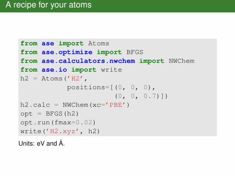
A recipe for your atoms
from ase import Atomsfrom ase.optimize import BFGSfrom ase.calculators.nwchem import NWChemfrom ase.io import writeh2 = Atoms(’H2’,
positions=[(0, 0, 0),(0, 0, 0.7)])
h2.calc = NWChem(xc=’PBE’)opt = BFGS(h2)opt.run(fmax=0.02)write(’H2.xyz’, h2)
Units: eV and Å.
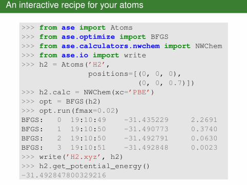
An interactive recipe for your atoms
>>> from ase import Atoms>>> from ase.optimize import BFGS>>> from ase.calculators.nwchem import NWChem>>> from ase.io import write>>> h2 = Atoms(’H2’,
positions=[(0, 0, 0),(0, 0, 0.7)])
>>> h2.calc = NWChem(xc=’PBE’)>>> opt = BFGS(h2)>>> opt.run(fmax=0.02)BFGS: 0 19:10:49 -31.435229 2.2691BFGS: 1 19:10:50 -31.490773 0.3740BFGS: 2 19:10:50 -31.492791 0.0630BFGS: 3 19:10:51 -31.492848 0.0023>>> write(’H2.xyz’, h2)>>> h2.get_potential_energy()-31.492847800329216
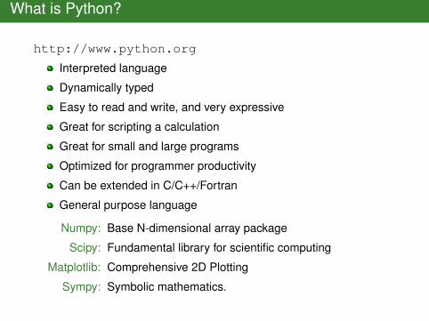
What is Python?
http://www.python.org
Interpreted language
Dynamically typed
Easy to read and write, and very expressive
Great for scripting a calculation
Great for small and large programs
Optimized for programmer productivity
Can be extended in C/C++/Fortran
General purpose language
Numpy: Base N-dimensional array package
Scipy: Fundamental library for scientific computing
Matplotlib: Comprehensive 2D Plotting
Sympy: Symbolic mathematics.
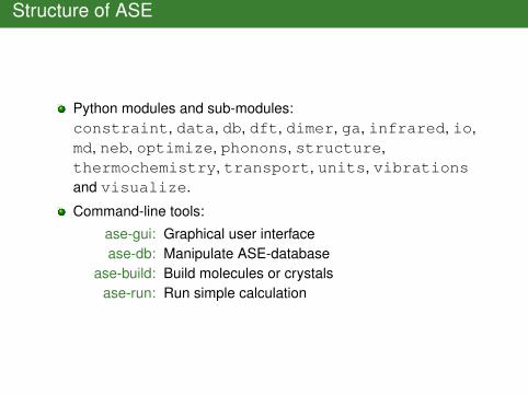
Structure of ASE
Python modules and sub-modules:constraint, data, db, dft, dimer, ga, infrared, io,md, neb, optimize, phonons, structure,thermochemistry, transport, units, vibrationsand visualize.
Command-line tools:
ase-gui: Graphical user interfacease-db: Manipulate ASE-database
ase-build: Build molecules or crystalsase-run: Run simple calculation
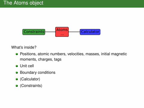
The Atoms object
Atoms...Constraints Calculator
What’s inside?
Positions, atomic numbers, velocities, masses, initial magneticmoments, charges, tags
Unit cell
Boundary conditions
(Calculator)
(Constraints)
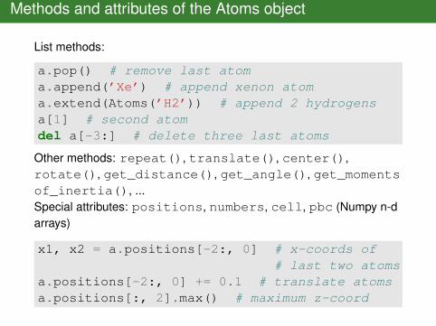
Methods and attributes of the Atoms object
List methods:
a.pop() # remove last atoma.append(’Xe’) # append xenon atoma.extend(Atoms(’H2’)) # append 2 hydrogensa[1] # second atomdel a[-3:] # delete three last atoms
Other methods: repeat(), translate(), center(),rotate(), get_distance(), get_angle(), get_momentsof_inertia(), ...Special attributes: positions, numbers, cell, pbc (Numpy n-darrays)
x1, x2 = a.positions[-2:, 0] # x-coords of# last two atoms
a.positions[-2:, 0] += 0.1 # translate atomsa.positions[:, 2].max() # maximum z-coord
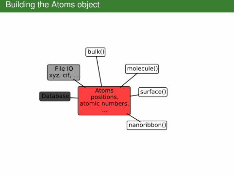
Building the Atoms object
Atomspositions,
atomic numbers,...
File IOxyz, cif, ...
Database
bulk()
molecule()
nanoribbon()
surface()
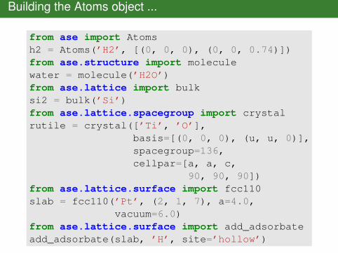
Building the Atoms object ...
from ase import Atomsh2 = Atoms(’H2’, [(0, 0, 0), (0, 0, 0.74)])from ase.structure import moleculewater = molecule(’H2O’)from ase.lattice import bulksi2 = bulk(’Si’)from ase.lattice.spacegroup import crystalrutile = crystal([’Ti’, ’O’],
basis=[(0, 0, 0), (u, u, 0)],spacegroup=136,cellpar=[a, a, c,
90, 90, 90])from ase.lattice.surface import fcc110slab = fcc110(’Pt’, (2, 1, 7), a=4.0,
vacuum=6.0)from ase.lattice.surface import add_adsorbateadd_adsorbate(slab, ’H’, site=’hollow’)
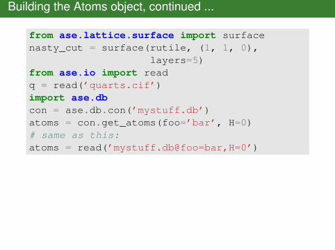
Building the Atoms object, continued ...
from ase.lattice.surface import surfacenasty_cut = surface(rutile, (1, 1, 0),
layers=5)from ase.io import readq = read(’quarts.cif’)import ase.dbcon = ase.db.con(’mystuff.db’)atoms = con.get_atoms(foo=’bar’, H=0)# same as this:atoms = read(’mystuff.db@foo=bar,H=0’)
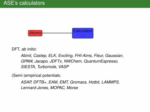
ASE’s calculators
Atoms Calculator...
DFT, ab initio:
Abinit, Castep, ELK, Exciting, FHI-Aims, Fleur, Gaussian,GPAW, Jacapo, JDFTx, NWChem, QuantumEspresso,SIESTA, Turbomole, VASP
(Semi-)empirical potentials:
ASAP, DFTB+, EAM, EMT, Gromacs, Hotbit, LAMMPS,Lennard-Jones, MOPAC, Morse
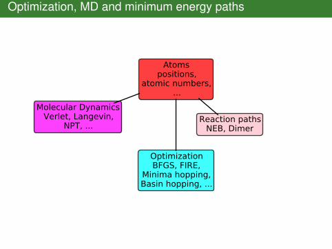
Optimization, MD and minimum energy paths
Atomspositions,
atomic numbers,...
Molecular DynamicsVerlet, Langevin,
NPT, ...
OptimizationBFGS, FIRE,
Minima hopping,Basin hopping, ...
Reaction pathsNEB, Dimer
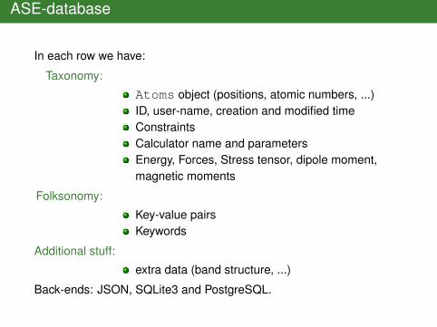
ASE-database
In each row we have:
Taxonomy:
Atoms object (positions, atomic numbers, ...)ID, user-name, creation and modified timeConstraintsCalculator name and parametersEnergy, Forces, Stress tensor, dipole moment,magnetic moments
Folksonomy:
Key-value pairsKeywords
Additional stuff:
extra data (band structure, ...)
Back-ends: JSON, SQLite3 and PostgreSQL.
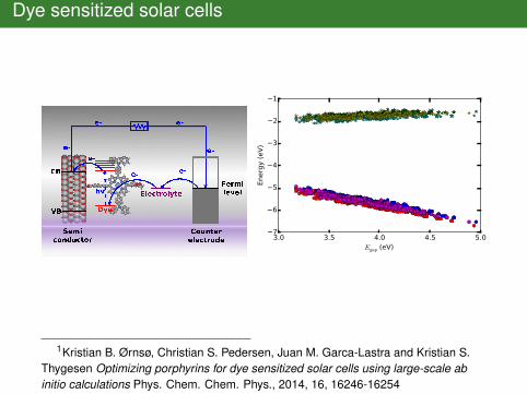
Dye sensitized solar cells
3.0 3.5 4.0 4.5 5.0Egap (eV)
7
6
5
4
3
2
1
Ener
gy (e
V)
1Kristian B. Ørnsø, Christian S. Pedersen, Juan M. Garca-Lastra and Kristian S.Thygesen Optimizing porphyrins for dye sensitized solar cells using large-scale abinitio calculations Phys. Chem. Chem. Phys., 2014, 16, 16246-16254
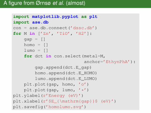
A figure from Ørnsø et al. (almost)
import matplotlib.pyplot as pltimport ase.dbcon = ase.db.connect(’dssc.db’)for M in [’Zn’, ’TiO’, ’H2’]:
gap = []homo = []lumo = []for dct in con.select(metal=M,
anchor=’EthynPhA’):gap.append(dct.E_gap)homo.append(dct.E_HOMO)lumo.append(dct.E_LUMO)
plt.plot(gap, homo, ’o’)plt.plot(gap, lumo, ’*’)
plt.ylabel(r’Energy (eV)’)plt.xlabel(r’$E_{\mathrm{gap}}$ (eV)’)plt.savefig(’homolumo.svg’)
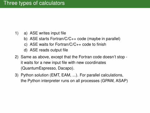
Three types of calculators
1) a) ASE writes input fileb) ASE starts Fortran/C/C++ code (maybe in parallel)c) ASE waits for Fortran/C/C++ code to finishd) ASE reads output file
2) Same as above, except that the Fortran code doesn’t stop -it waits for a new input file with new coordinates(QuantumEspresso, Dacapo).
3) Python solution (EMT, EAM, ...). For parallel calculations,the Python interpreter runs on all processes (GPAW, ASAP)
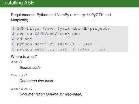
Installing ASE
Requirements: Python and NumPy (ase-gui: PyGTK andMatplotlib)
$ SVN=https://svn.fysik.dtu.dk/projects$ svn co $SVN/ase/trunk ase$ cd ase$ python setup.py install --user$ python setup.py test # takes 1 min.
Where is what?ase/:
Source code.
tools/:Command-line tools
ase/doc/:Documentation (source for web-page)
Questions
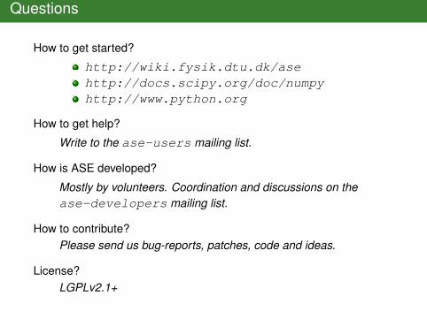
How to get started?
http://wiki.fysik.dtu.dk/asehttp://docs.scipy.org/doc/numpyhttp://www.python.org
How to get help?
Write to the ase-users mailing list.
How is ASE developed?
Mostly by volunteers. Coordination and discussions on thease-developers mailing list.
How to contribute?Please send us bug-reports, patches, code and ideas.
License?LGPLv2.1+
Thanks
Andrew Peterson, Anthony Goodrow, Ask Hjorth Larsen, CarstenRostgaard, Christian Glinsvad, David Landis, Elvar Örn Jónsson, EricHermes, Felix Hanke, Gaël Donval, George Tritsaris, Glen Jenness,Heine Anton Hansen, Ivano Eligio Castelli, Jakob Blomquist, JakobSchiøtz, Janne Blomqvist, Janosch Michael Rauba, Jens JørgenMortensen, Jesper Friis, Jesper Kleis, Jess Wellendorff Pedersen,Jingzhe Chen, John Kitchin, Jon Bergmann Maronsson, Jonas Bjork,Jussi Enkovaara, Karsten Wedel Jacobsen, Kristen Kaasbjerg, KristianBaruel Ørnsø, Lars Grabow, Lars Pastewka, Lasse Vilhelmsen, MarcinDulak, Marco Vanin, Markus Kaukonen, Mattias Slabanja, MichaelWalter, Mikkel Strange, Poul Georg Moses, Rolf Würdemann, SteenLysgaard, Stephan Schenk, Tao Jiang, Thomas Olsen, TristanMaxson, Troels Kofoed Jacobsen, ...
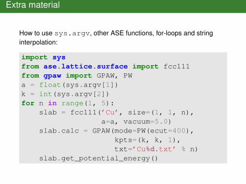
Extra material
How to use sys.argv, other ASE functions, for-loops and stringinterpolation:
import sysfrom ase.lattice.surface import fcc111from gpaw import GPAW, PWa = float(sys.argv[1])k = int(sys.argv[2])for n in range(1, 5):
slab = fcc111(’Cu’, size=(1, 1, n),a=a, vacuum=5.0)
slab.calc = GPAW(mode=PW(ecut=400),kpts=(k, k, 1),txt=’Cu%d.txt’ % n)
slab.get_potential_energy()