Embed Size (px)
Citation preview

Modeling and Simulation in Python
Version 1.2.4


Modeling and Simulation in Python
Version 1.2.4
Allen B. Downey
Green Tea Press
Needham, Massachusetts

Copyright © 2017 Allen B. Downey.
Green Tea Press
9 Washburn Ave
Needham MA 02492
Permission is granted to copy, distribute, transmit and adapt this work under a
Creative Commons Attribution-NonCommercial-ShareAlike 4.0 International
License: http://modsimpy.com/license.
If you are interested in distributing a commercial version of this work, please
contact the author.
The LATEX source and code for this book is available from
https://github.com/AllenDowney/ModSimPy

iv

Contents
Preface xi
0.1 Can modeling be taught? . . . . . . . . . . . . . . . . . . . . xiii
0.2 How much programming do I need? . . . . . . . . . . . . . . xiv
0.3 How much math and science do I need? . . . . . . . . . . . . xv
0.4 Getting started . . . . . . . . . . . . . . . . . . . . . . . . . xvi
0.5 Installing Python and the libraries . . . . . . . . . . . . . . . xvi
0.6 Copying my files . . . . . . . . . . . . . . . . . . . . . . . . . xvii
0.7 Running Jupyter . . . . . . . . . . . . . . . . . . . . . . . . xviii
1 Modeling 1
1.1 The falling penny myth . . . . . . . . . . . . . . . . . . . . . 1
1.2 Computation . . . . . . . . . . . . . . . . . . . . . . . . . . 3
1.3 Modeling a bike share system . . . . . . . . . . . . . . . . . 4
1.4 Plotting . . . . . . . . . . . . . . . . . . . . . . . . . . . . . 6
1.5 Defining functions . . . . . . . . . . . . . . . . . . . . . . . . 7
1.6 Parameters . . . . . . . . . . . . . . . . . . . . . . . . . . . . 8
1.7 Print statements . . . . . . . . . . . . . . . . . . . . . . . . . 10
1.8 If statements . . . . . . . . . . . . . . . . . . . . . . . . . . . 11
1.9 For loops . . . . . . . . . . . . . . . . . . . . . . . . . . . . . 14
1.10 Under the hood . . . . . . . . . . . . . . . . . . . . . . . . . 14

vi CONTENTS
2 Simulation 17
2.1 Iterative modeling . . . . . . . . . . . . . . . . . . . . . . . . 17
2.2 More than one System object . . . . . . . . . . . . . . . . . 18
2.3 Documentation . . . . . . . . . . . . . . . . . . . . . . . . . 20
2.4 Negative bikes . . . . . . . . . . . . . . . . . . . . . . . . . . 21
2.5 Comparison operators . . . . . . . . . . . . . . . . . . . . . . 23
2.6 Metrics . . . . . . . . . . . . . . . . . . . . . . . . . . . . . . 24
2.7 Functions that return values . . . . . . . . . . . . . . . . . . 26
2.8 Two kinds of parameters . . . . . . . . . . . . . . . . . . . . 27
2.9 Loops and arrays . . . . . . . . . . . . . . . . . . . . . . . . 28
2.10 Sweeping parameters . . . . . . . . . . . . . . . . . . . . . . 29
2.11 Incremental development . . . . . . . . . . . . . . . . . . . . 30
3 Explanation 31
3.1 World Population Data . . . . . . . . . . . . . . . . . . . . . 31
3.2 Plotting . . . . . . . . . . . . . . . . . . . . . . . . . . . . . 34
3.3 Constant growth model . . . . . . . . . . . . . . . . . . . . . 34
3.4 Simulation . . . . . . . . . . . . . . . . . . . . . . . . . . . . 36
3.5 Now with System objects . . . . . . . . . . . . . . . . . . . . 38
3.6 Proportional growth model . . . . . . . . . . . . . . . . . . . 39
3.7 Factoring out the update function . . . . . . . . . . . . . . . 41
3.8 Combining birth and death . . . . . . . . . . . . . . . . . . . 42
3.9 Quadratic growth . . . . . . . . . . . . . . . . . . . . . . . . 43
3.10 Equilibrium . . . . . . . . . . . . . . . . . . . . . . . . . . . 46
3.11 Disfunctions . . . . . . . . . . . . . . . . . . . . . . . . . . . 46
4 Prediction 51

CONTENTS vii
4.1 Generating projections . . . . . . . . . . . . . . . . . . . . . 51
4.2 Comparing projections . . . . . . . . . . . . . . . . . . . . . 54
4.3 Recurrence relations . . . . . . . . . . . . . . . . . . . . . . 55
4.4 Differential equations . . . . . . . . . . . . . . . . . . . . . . 57
4.5 Analysis and simulation . . . . . . . . . . . . . . . . . . . . 59
4.6 Analysis with WolframAlpha . . . . . . . . . . . . . . . . . . 60
4.7 Analysis with SymPy . . . . . . . . . . . . . . . . . . . . . . 61
4.8 Differential equations in SymPy . . . . . . . . . . . . . . . . 62
4.9 Solving the quadratic growth model . . . . . . . . . . . . . . 63
4.10 Summary . . . . . . . . . . . . . . . . . . . . . . . . . . . . 64
4.11 DataFrames and Series . . . . . . . . . . . . . . . . . . . . . 65
4.12 One queue or two? . . . . . . . . . . . . . . . . . . . . . . . 66
5 Design 71
5.1 The Freshman Plague . . . . . . . . . . . . . . . . . . . . . . 71
5.2 The SIR model . . . . . . . . . . . . . . . . . . . . . . . . . 72
5.3 The SIR equations . . . . . . . . . . . . . . . . . . . . . . . 73
5.4 Implementation . . . . . . . . . . . . . . . . . . . . . . . . . 74
5.5 The update function . . . . . . . . . . . . . . . . . . . . . . 76
5.6 Running the simulation . . . . . . . . . . . . . . . . . . . . . 77
5.7 Collecting the results . . . . . . . . . . . . . . . . . . . . . . 78
5.8 Now with a TimeFrame . . . . . . . . . . . . . . . . . . . . . 80
5.9 Metrics . . . . . . . . . . . . . . . . . . . . . . . . . . . . . . 81
5.10 Immunization . . . . . . . . . . . . . . . . . . . . . . . . . . 82
5.11 Hand washing . . . . . . . . . . . . . . . . . . . . . . . . . . 85
5.12 Optimization . . . . . . . . . . . . . . . . . . . . . . . . . . 88

viii CONTENTS
5.13 Under the hood . . . . . . . . . . . . . . . . . . . . . . . . . 90
6 Analysis 91
6.1 Unpack . . . . . . . . . . . . . . . . . . . . . . . . . . . . . . 91
6.2 Sweeping beta . . . . . . . . . . . . . . . . . . . . . . . . . . 92
6.3 Sweeping gamma . . . . . . . . . . . . . . . . . . . . . . . . 94
6.4 Nondimensionalization . . . . . . . . . . . . . . . . . . . . . 96
6.5 Contact number . . . . . . . . . . . . . . . . . . . . . . . . . 98
6.6 Analysis and simulation . . . . . . . . . . . . . . . . . . . . 100
7 Thermal systems 103
7.1 The coffee cooling problem . . . . . . . . . . . . . . . . . . . 103
7.2 Temperature and heat . . . . . . . . . . . . . . . . . . . . . 104
7.3 Heat transfer . . . . . . . . . . . . . . . . . . . . . . . . . . 105
7.4 Newton’s law of cooling . . . . . . . . . . . . . . . . . . . . . 106
7.5 Implementation . . . . . . . . . . . . . . . . . . . . . . . . . 107
7.6 Using fsolve . . . . . . . . . . . . . . . . . . . . . . . . . . . 109
7.7 Mixing liquids . . . . . . . . . . . . . . . . . . . . . . . . . . 112
7.8 Mix first or last? . . . . . . . . . . . . . . . . . . . . . . . . 113
7.9 Optimization . . . . . . . . . . . . . . . . . . . . . . . . . . 114
7.10 Analysis . . . . . . . . . . . . . . . . . . . . . . . . . . . . . 116
8 Pharmacokinetics 119
8.1 The glucose-insulin system . . . . . . . . . . . . . . . . . . . 119
8.2 The glucose minimal model . . . . . . . . . . . . . . . . . . . 120
8.3 Data . . . . . . . . . . . . . . . . . . . . . . . . . . . . . . . 123
8.4 Interpolation . . . . . . . . . . . . . . . . . . . . . . . . . . . 123

CONTENTS ix
8.5 Implementation . . . . . . . . . . . . . . . . . . . . . . . . . 125
8.6 Numerical solution of differential equations . . . . . . . . . . 128
8.7 Least squares . . . . . . . . . . . . . . . . . . . . . . . . . . 130
8.8 Interpreting parameters . . . . . . . . . . . . . . . . . . . . . 132
8.9 The insulin minimal model . . . . . . . . . . . . . . . . . . . 135
9 Projectiles 137
9.1 Newton’s second law of motion . . . . . . . . . . . . . . . . . 137
9.2 Dropping pennies . . . . . . . . . . . . . . . . . . . . . . . . 139
9.3 Onto the sidewalk . . . . . . . . . . . . . . . . . . . . . . . . 142
9.4 With air resistance . . . . . . . . . . . . . . . . . . . . . . . 143
9.5 Implementation . . . . . . . . . . . . . . . . . . . . . . . . . 144
9.6 Dropping quarters . . . . . . . . . . . . . . . . . . . . . . . . 146
10 Two dimensions 151
10.1 The Manny Ramirez problem . . . . . . . . . . . . . . . . . 151
10.2 Vectors . . . . . . . . . . . . . . . . . . . . . . . . . . . . . . 152
10.3 Modeling baseball flight . . . . . . . . . . . . . . . . . . . . . 155
10.4 Trajectories . . . . . . . . . . . . . . . . . . . . . . . . . . . 158
10.5 Finding the range . . . . . . . . . . . . . . . . . . . . . . . . 160
10.6 Optimization . . . . . . . . . . . . . . . . . . . . . . . . . . 162
10.7 Finishing off the problem . . . . . . . . . . . . . . . . . . . . 164
11 Rotation 165
11.1 The physics of toilet paper . . . . . . . . . . . . . . . . . . . 166
11.2 Implementation . . . . . . . . . . . . . . . . . . . . . . . . . 167
11.3 Analysis . . . . . . . . . . . . . . . . . . . . . . . . . . . . . 171

x CONTENTS
11.4 Torque . . . . . . . . . . . . . . . . . . . . . . . . . . . . . . 172
11.5 Moment of inertia . . . . . . . . . . . . . . . . . . . . . . . . 173
11.6 Unrolling . . . . . . . . . . . . . . . . . . . . . . . . . . . . . 175
11.7 Simulating a yo-yo . . . . . . . . . . . . . . . . . . . . . . . 179
12 Second order systems 183
Index 185

Preface
This book is about modeling and simulation of physical systems. The following
diagram shows what I mean by “modeling”:
Abstraction
Analysis
Simulation
Valid
ati on
Measurement
Model
System
Pred
ict ion
Data
Starting in the lower left, the system is something in the real world we are
interested in. Often, it is something complicated, so we have to decide which
details can be simplified or abstracted away.
The result of abstraction is a model that includes the features we think are
essential. A model can be represented in the form of diagrams and equations,
which can be used for mathematical analysis. It can also be implemented in
the form of a computer program, which can run simulations.
The result of analysis and simulation can be a prediction about what the

xii Chapter 0 Preface
system will do, an explanation of why it behaves the way it does, or a design
intended to achieve a purpose.
We can validate predictions and test designs by taking measurements from
the real world and comparing the data we get with the results from analysis
and simulation.
This process is almost always iterative: for any physical system, there are
many possible models, each one including and excluding different features, or
including different levels of detail. The goal of the modeling process is to find
the model best suited to its purpose (prediction, explanation, or design).
Sometimes the best model is the most detailed. If we include more features,
the model is more realistic, and we expect its predictions to be more accurate.
But often a simpler model is better. If we include only the essential features
and leave out the rest, we get models that are easier to work with, and the
explanations they provide can be clearer and more compelling.
As an example, suppose someone asked you why the orbit of the Earth is nearly
elliptical. If you model the Earth and Sun as point masses (ignoring their
actual size), compute the gravitational force between them using Newton’s
law of universal gravitation, and compute the resulting orbit using Newton’s
laws of motion, you can show that the result is an ellipse.
Of course, the actual orbit of Earth is not a perfect ellipse, because of the
gravitational forces of the Moon, Jupiter, and other objects in the solar system,
and because Newton’s laws of motion are only approximately true (they don’t
take into account relativistic effects).
But adding these features to the model would not improve the explanation;
more detail would only be a distraction from the fundamental cause. However,
if the goal is to predict the position of the Earth with great precision, including
more details might be necessary.
So choosing the best model depends on what the model is for. It is usually a
good idea to start with a simple model, even if it is likely to be too simple,
and test whether it is good enough for its purpose. Then you can add features
gradually, starting with the ones you expect to be most essential.

0.1 Can modeling be taught? xiii
Comparing the results of successive models provides a form of internal vali-
dation, so you can catch conceptual, mathematical, and software errors. And
by adding and removing features, you can tell which ones have the biggest
effect on the results, and which can be ignored.
0.1 Can modeling be taught?
These essential modeling skills — abstraction, analysis, simulation, and vali-
dation — are central in engineering, natural sciences, social sciences, medicine,
and many other fields. Some students learn these skills implicitly, but in most
schools they are not taught explicitly, and students get little practice. That’s
the problem this book is meant to address.
At Olin College, we use this book in a class called Modeling and Simulation,
which all students take in their first semester. My colleagues, John Geddes
and Mark Somerville, and I developed this class and taught it for the first time
in 2009.
It is based on our belief that modeling should be taught explicitly, early, and
throughout the curriculum. It is also based on our conviction that computation
is an essential part of this process.
If students are limited to the mathematical analysis they can do by hand, they
are restricted to a small number of simple physical systems, like a projectile
moving in a vacuum or a block on a frictionless plane.
And they will only work with bad models; that is, models that are too simple
for their purpose. In nearly every mechanical system, air resistance and friction
are essential features; if we ignore them, our predictions will be wrong and our
designs won’t work.
In most freshman physics classes, students don’t make modeling decisions;
sometimes they are not even aware of the decisions that have been made for
them. Our goal is to teach, and for students to practice, the entire modeling
process.

xiv Chapter 0 Preface
0.2 How much programming do I need?
If you have never programmed before, you should be able to read this book,
understand it, and do the exercises. I will do my best to explain everything you
need to know; in particular, I have chosen carefully the vocabulary I introduce,
and I try to define each term the first time it it used. If you find that I have
used a term without defining it, let me know.
If you have programmed before, you will have an easier time getting started,
but you might be uncomfortable in some places. I take an approach to pro-
gramming you have probably not seen before.
Most programming classes1 have two big problems:
1. They go “bottom up”, starting with basic language features and gradu-
ally adding more powerful tools. As a result, it takes a long time before
students can do anything more interesting than convert Fahrenheit to
Celsius.
2. They have no context. Students learn to program with no particular goal
in mind, so the exercises span an incoherent collection of topics, and the
projects tend to be unmotivated.
In this book, you learn to program with an immediate goal in mind: writing
simulations of physical systems. And we proceed “top down”, by which I mean
we use professional-strength data structures and language features right away.
In particular, we use the following Python libraries:
� NumPy for basic numerical computation (see http://www.numpy.org/).
� SciPy for scientific computation (see http://www.scipy.org/).
� matplotlib for visualization (see http://matplotlib.org/).
� pandas for working with data (see http://pandas.pydata.org/).
� SymPy for symbolic computation, (see http://www.sympy.org).
� Pint for units like kilograms and meters (see http://pint.readthedocs.
io).
1Including many I have taught.

0.3 How much math and science do I need? xv
� Jupyter for reading, running, and developing code (see http://jupyter.
org).
These tools let you work on more interesting programs sooner, but there are
some drawbacks: they can be hard to use, and it can be challenging to keep
track of which library does what and how they interact.
I have tried to mitigate these problems by providing a library, called modsim,
that makes it easier to get started with these tools, and provides some addi-
tional capabilities.
Some features in the modsim library are like training wheels; at some point you
will probably stop using them and start working with the underlying libraries
directly. Other features you might find useful the whole time you are working
through the book, or even later.
I encourage you to read the the modsim library code. Most of it is not com-
plicated, and I tried to make it readable. Particularly if you have some pro-
gramming experience, you might learn something by reverse-engineering my
designs.
0.3 How much math and science do I need?
I assume that you have studied calculus. You should know what derivatives
and integrals are, but that’s about all. In particular, you don’t need to know
(or remember) much about finding derivatives or integrals of functions analyt-
ically. If you know the derivative of x2 and you can integrate 2x dx, that will
do it2.
More importantly you should understand what those concepts mean; but if
you don’t, this book might help you figure it out.
You don’t have to know anything about differential equations.
As for science, we will cover topics from a variety of fields, including demogra-
phy, epidemiology, medicine, thermodynamics, and mechanics. For the most
part, I don’t assume you know anything about these topics. In fact, one of the
2And if you noticed that those two questions answer each other, even better.

xvi Chapter 0 Preface
skills you need to do modeling is the ability to learn enough about new fields
to develop models and simulations.
When we get to mechanics, I assume you understand the relationship between
position, velocity, and acceleration, and that you are familiar with Newton’s
laws of motion, especially the second law, which is often expressed as F = ma
(force equals mass times acceleration).
I think that’s everything you need, but if you find that I left something out,
please let me know.
0.4 Getting started
To run the examples and work on the exercises in this book, you will need to
be able to:
1. Install Python on your computer, along with the libraries we will use.
2. Copy my files onto your computer.
3. Run Jupyter, which is a tool for running and writing programs, and load
a notebook, which is a file that contains code and text.
The next three sections provide details for these steps. I wish there were an
easier way to get started; it’s regrettable that you have to do so much work
before you write your first program. Be persistent!
0.5 Installing Python and the libraries
You might already have Python installed on your computer, but you might
not have the latest version. To use the code in this book, you need Python
3.6, or later. Even if you have the latest version, you probably don’t have all
of the libraries we need.
You could update Python and install these libraries, but I strongly recom-
mend that you don’t go down that road. I think you will find it easier to use

0.6 Copying my files xvii
Anaconda, which is a free Python distribution that includes all the libraries
you need for this book (and lots more).
Anaconda is available for Linux, macOS, and Windows. By default, it puts all
files in your home directory, so you don’t need administrator (root) permission
to install it, and if you have a version of Python already, Anaconda will not
remove or modify it.
[Detailed instructions coming soon.]
0.6 Copying my files
The code for this book is available from https://github.com/AllenDowney/
ModSimPy, which is a Git repository. Git is a software tool that helps you
keep track of the programs and other files that make up a project. A collection
of files under Git’s control is called a repository3. GitHub is a hosting service
that provides storage for Git repositories and a convenient web interface.
There are several ways you can copy the files from my repository to your
computer.
If you don’t want to use Git at all, you can download my files in a Zip archive
from http://modsimpy.com/zip. Then you need a program like WinZip or
gzip to unpack the Zip file.
To use Git, you need a Git client, which is a program that manages git repos-
itories. If you have not used Git before, I recommend GitHub Desktop, which
is a simple graphical Git client. You can download it from https://desktop.
github.com. Currently, GitHub Desktop is not available for Linux. On Linux,
I suggest using the Git command-line client. Installation instructions are at
http://modsimpy.com/git.
Once you have a Git client, you can use it to copy files from my repository to
your computer, which is called cloning in Git’s vocabulary. If you are using
a Command-line git client, type
git clone https://github.com/AllenDowney/ModSimPy
3The really cool kids call it a “repo”.
xviii Chapter 0 Preface
You don’t need a GitHub account to do this, but you won’t be able to write
your changes back to GitHub.
If you want to use GitHub to keep track of the code you write while you are
using this book, you can make of a copy of my repository on GitHub, which
is called forking. If you don’t already have a GitHub account, you’ll need to
create one.
Use a browser to view the homepage of my repository at https://github.
com/AllenDowney/ModSimPy. You should see a gray button in the upper right
that says Fork. If you press it, GitHub will create a copy of my repository that
belongs to you. Then you can clone your repository like this:
git clone https://github.com/YourGitHubUserName/ModSimPy
Of course, you should replace YourGitHubUserName with your GitHub user
name.
0.7 Running Jupyter
The code for each chapter, and starter code for the exercises, is in Jupyter
notebooks. If you have not used Jupyter before, you can read about it at
http://jupyter.org.
[Jupyter instructions coming soon.]
Contributor List
If you have a suggestion or correction, send it to [email protected].
Or if you are a Git user, send me a pull request!
If I make a change based on your feedback, I will add you to the contributor
list, unless you ask to be omitted.
If you include at least part of the sentence the error appears in, that makes it
easy for me to search. Page and section numbers are fine, too, but not as easy
to work with. Thanks!

0.7 Running Jupyter xix
� I am grateful to John Geddes and Mark Somerville for their early col-
laboration with me to create Modeling at Simulation, the class at Olin
College this book is based on.
� My early work on this book benefited from conversations with my amaz-
ing colleagues at Olin College, including John Geddes, Alison Wood,
Chris Lee, and Jason Woodard.
� I am grateful to Lisa Downey and Jason Woodard for their thoughtful
and careful copy editing.

xx Chapter 0 Preface

Chapter 1
Modeling
The world is a complicated place. In order to make sense of it, we use models,
which are generally smaller and simpler than the thing we want to study. The
word “model” means different things in different contexts, so it is hard to
define except by example.
Some models are actual objects, like a scale model of a car, which has the
same shape as the car, but smaller. Scale models are often useful for testing
properties of mechanical systems, like air resistance.
This book is about mathematical models, which are ideas, not objects. If
you studied Newton’s laws of motion, what you learned is a mathematical
model of how objects move in space when forces are applied to them.
1.1 The falling penny myth
Let’s see an example of how models are used. You might have heard that a
penny dropped from the top of the Empire State Building would be going so
fast when it hit the pavement that it would be embedded in the concrete; or
if it hit a person, it would break their skull.
We can test this myth by making and analyzing a model. To get started, I’ll
assume that the effect of air resistance is small. This will turn out to be a bad
assumption, but bear with me. If air resistance is negligible, the primary force

2 Chapter 1 Modeling
acting on the penny is gravity, which causes the penny to accelerate downward.
If the initial velocity is 0, the velocity after t seconds is at, and the height the
penny has dropped at t is
h = at2/2
Using algebra, we can solve for t:
t =√
2h/a
Plugging in the acceleration of gravity, a = 9.8 m/s2 and the height of the
Empire State Building, h = 381 m, we get t = 8.8 s. Then computing v = at
we get a velocity on impact of 86 m/s, which is about 190 miles per hour. That
sounds like it could hurt.
Of course, these results are not exact because the model is based on simplifi-
cations. For example, we assume that gravity is constant. In fact, the force
of gravity is different on different parts of the globe, and gets weaker as you
move away from the surface. But these differences are small, so ignoring them
is probably a good choice for this scenario.
On the other hand, ignoring air resistance is not a good choice. Once the penny
gets to about 18 m/s, the upward force of air resistance equals the downward
force of gravity, so the penny stops accelerating. After that, it doesn’t matter
how far the penny falls; it hits the sidewalk (or your head) at about 18 m/s,
much less than 86 m/s, as the simple model predicts.
The statistician George Box famously said “All models are wrong, but some
are useful.” He was talking about statistical models, but his wise words apply
to all kinds of models. Our first model, which ignores air resistance, is very
wrong, and probably not useful. The second model is also wrong, but much
better, and probably good enough to refute the myth.
The television show Mythbusters has tested the myth of the falling penny more
carefully; you can view the results at http://modsimpy.com/myth. Their work
is based on a mathematical model of motion, measurements to determine the
force of air resistance on a penny, and a physical model of a human head.

1.2 Computation 3
1.2 Computation
There are (at least) two ways to work with mathematical models, analysis
and simulation. Analysis often involves algebra and other kinds of symbolic
manipulation. Simulation often involves computers.
In this book we do some analysis and a lot of simulation; along the way, I
discuss the pros and cons of each. The primary tools we use for simulation are
the Python programming language and Jupyter, which is an environment for
writing and running programs.
As a first example, I’ll show you how I computed the results from the previ-
ous section using Python. You can view this example at http://modsimpy.
com/chap00. For instructions on downloading and running the code, see Sec-
tion 0.4.
First I’ll create a variable to represent acceleration.
a = 9.8 * meter / second**2
A variable is a name that corresponds to a value. In this example, the name is
a and the value is the number 9.8 multiplied by the units meter / second**2.
This example demonstrates some of the symbols Python uses to perform math-
ematical operations:
Operation Symbol
Addition +
Subtraction -
Multiplication *
Division /
Exponentiation **
Next, we can compute the time it takes for the penny to drop 381 m, the height
of the Empire State Building.
h = 381 * meter
t = sqrt(2 * h / a)
4 Chapter 1 Modeling
These lines create two more variables: h gets the height of the building in
meters; t gets the time, in seconds, for the penny to fall to the sidewalk. sqrt
is a function that computes square roots. Python keeps track of units, so the
result, t, has the correct units, seconds.
Finally, we can compute the velocity of the penny after t seconds:
v = a * t
The result is about 86 m/s, again with the correct units.
This example demonstrates analysis and computation using Python. Next
we’ll see an example of simulation.
1.3 Modeling a bike share system
You can view the code for the rest of this chapter at http://modsimpy.
com/chap01. For instructions on downloading and running the code, see Sec-
tion 0.4.
Imagine a bike share system for students traveling between Olin College and
Wellesley College, which are about 3 miles apart in eastern Massachusetts.
This example demonstrates the features of Python we’ll use to develop com-
putational simulations of real-world systems. Along the way, I will make deci-
sions about how to model the system. In the next chapter we’ll review these
decisions.
Suppose the system contains 12 bikes and two bike racks, one at Olin and one
at Wellesley, each with the capacity to hold 12 bikes.
As students arrive, check out a bike, and ride to the other campus, the number
of bikes in each location changes. In the simulation, we’ll need to keep track of
where the bikes are. To do that, I’ll create a System object, which is defined
in the modsim library.
Before we can use the library, we have to import it:

1.3 Modeling a bike share system 5
from modsim import *
This line of code is an import statement that tells Python to read the file
modsim.py and make the functions it defines available.
Functions in the modsim.py library include sqrt, which we used in the previous
section, and System, which we are using now. System creates a System object,
which is a collection of system variables.
bikeshare = System(olin=10, wellesley=2)
In this example, the system variables are olin and wellesley and they repre-
sent the number of bikes at Olin and Wellesley. The initial values are 10 and
2, indicating that there are 10 bikes at Olin and 2 at Wellesley. The System
object created by System is assigned to a new variable named bikeshare.
We can read the variables inside a System object using the dot operator,
like this:
bikeshare.olin
The result is the value 10. Similarly, for:
bikeshare.wellesley
The result is 2. If you forget what variables a system object has, you can just
type the name:
bikeshare
The result looks like a table with the variable names and their values:
value
olin 10
wellesley 2
The system variables and their values make up the state of the system. We
can update the state by assigning new values to the variables. For example,
6 Chapter 1 Modeling
if a student moves a bike from Olin to Wellesley, we can figure out the new
values and assign them:
bikeshare.olin = 9
bikeshare.wellesley = 3
Or we can use update operators, -= and += to subtract 1 from olin and
add 1 to wellesley:
bikeshare.olin -= 1
bikeshare.wellesley += 1
The result is the same either way.
1.4 Plotting
As the state of the system changes, it is often useful to plot the values of the
variables over time. The modsim library provides a function that creates a new
figure:
newfig()
In Jupyter, the behavior of this function depends on a command in the first
cell:
� If you want the figures to appear in the notebook, use
%matplotlib notebook
� If you want the figures to appear in separate windows, use
%matplotlib qt
These commands are not actually Python; they are so-called “magic com-
mands” that control the behavior of Jupyter.
The following lines plot the state of the system:

1.5 Defining functions 7
mark(bikeshare.olin, 'rs-')
mark(bikeshare.wellesley, 'bo-')
The mark function takes two values, called arguments:
� The first argument is the variable to plot. In this example, it’s a number,
but we’ll see later that mark can handle other objects, too.
� The second argument is a “style string” that determines what the plot
should look like. In general, a string is a sequence of letters, numbers,
and punctuation that appear in quotation marks. The style string 'rs-'
means we want red squares with lines between them; 'bo-' means we
want blue circles with lines.
The plotting functions in the modsim library are based on Matplotlib, which is
a Python library for generating figures. To learn more about these functions,
you can read the Matplotlib documentation. For more about style strings, see
http://modsimpy.com/plot.
1.5 Defining functions
So far we have used functions defined in modsim and other libraries. Now we’re
going to define our own functions.
When you are developing code in Jupyter, it is often efficient to write 1–2 lines
in each cell, test them to confirm they do what you intend, and then use them
to define a new function. For example, these lines move a bike from Olin to
Wellesley:
bikeshare.olin -= 1
bikeshare.wellesley += 1
Rather than repeat them every time a bike moves, we can define a new func-
tion:
def bike_to_wellesley():
bikeshare.olin -= 1
bikeshare.wellesley += 1
8 Chapter 1 Modeling
def is a special word in Python that indicates we are defining a new function.
The name of the function is bike_to_wellesley. The empty parentheses indi-
cate that this function takes no arguments. The colon indicates the beginning
of an indented code block.
The next two lines are the body of the function. They have to be indented;
by convention, the indentation is 4 spaces.
When you define a function, it has no immediate effect. The body of the func-
tion doesn’t run until you call the function. Here’s how to call this function:
bike_to_wellesley()
When you call this function, it updates the variables of the bikeshare object;
you can check by displaying or plotting the new state.
When you call a function that takes no arguments, you have to include the
empty parentheses. If you leave them out, like this:
bike_to_wellesley
Python looks up the name of the function and displays:
<function __main__.bike_to_wellesley>
This result indicates that bike_to_wellesley is a function. You don’t have
to know what __main__ means, but if you see something like this, it probably
means that you looked up a function but you didn’t actually run it. So don’t
forget the parentheses.
1.6 Parameters
Similarly, we can define a function that moves a bike from Wellesley to Olin:
def bike_to_olin():
bikeshare.wellesley -= 1
bikeshare.olin += 1

1.6 Parameters 9
And run it like this:
bike_to_olin()
One benefit of defining functions is that you avoid repeating chunks of code,
which makes programs smaller. Another benefit is that the name you give the
function documents what it does, which makes programs more readable.
In this example, there is one other benefit that might be even more important.
Putting these lines in a function makes the program more reliable because it
guarantees that when we decrease the number of bikes at Olin, we increase
the number of bikes at Wellesley. That way, we guarantee that the bikes in
the model are neither created nor destroyed!
However, now we have two functions that are nearly identical except for a
change of sign. Repeated code makes programs harder to work with, because
if we make a change, we have to make it in several places.
We can avoid that by defining a more general function that moves any number
of bikes in either direction:
def move_bike(n):
bikeshare.olin -= n
bikeshare.wellesley += n
The name in parentheses, n, is a parameter of the function. When we run
the function, the argument we provide gets assigned to the parameter. So if
we run move_bike like this:
move_bike(1)
It assigns the value of the argument, 1, to the parameter, n, and then runs the
body of the function. So the effect is the same as:
n = 1
bikeshare.olin -= n
bikeshare.wellesley += n
Which moves a bike from Olin to Wellesley. Similarly, if we call move_bike
like this:

10 Chapter 1 Modeling
move_bike(-1)
The effect is the same as:
n = -1
bikeshare.olin -= n
bikeshare.wellesley += n
Which moves a bike from Wellesley to Olin. Now that we have move_bike, we
can rewrite the other two functions to use it:
def bike_to_wellesley():
move_bike(1)
def bike_to_olin():
move_bike(-1)
If you define the same function name more than once, the new definition
replaces the old one.
1.7 Print statements
As you write more complicated programs, it is easy to lose track of what is
going on. One of the most useful tools for debugging is the print statement,
which displays text in the Jupyter notebook.
Normally when Jupyter runs the code in a cell, it displays the value of the last
line of code. For example, if you run:
bikeshare.olin
bikeshare.wellesley
Jupyter runs both lines of code, but it only displays the value of the second
line. If you want to display more than one value, you can use print statements:
print(bikeshare.olin)
print(bikeshare.wellesley)

1.8 If statements 11
print is a function, so it takes an argument in parentheses. It can also take a
sequence of arguments separated by commas, like this:
print(bikeshare.olin, bikeshare.wellesley)
In this example, the two values appear on the same line, separated by a space.
Print statements are also useful for debugging functions. For example, if you
add a print statement to move_bike, like this:
def move_bike(n):
print('Running move_bike with n =', n)
bikeshare.olin -= n
bikeshare.wellesley += n
The first argument of print is a string; the second is the value of n, which is
a number. Each time you run move_bike, it displays a message and the value
n.
1.8 If statements
The modsim library provides a function called flip that takes as an argument
a probability between 0 and 1:
flip(0.7)
The result is one of two values: True with probability 0.7 or False with
probability 0.3. If you run this function 100 times, you should to get True
about 70 times and False about 30 times. But the results are random, so
they might differ from these expectations.
True and False are special values defined by Python. Note that they are
not strings. There is a difference between True, which is a special value, and
'True', which is a string.
True and False are called boolean values because they are related to Boolean
algebra (http://modsimpy.com/boolean).

12 Chapter 1 Modeling
We can use boolean values to control the behavior of the program using an if
statement:
if flip(0.5):
print('heads')
If the result from flip is True, the program displays the string 'heads'.
Otherwise it does nothing.
The punctuation for if statements is similar to the punctuation for function
definitions: the first line has to end with a colon, and the lines inside the if
statement have to be indented.
Optionally, you can add an else clause to indicate what should happen if the
result is False:
if flip(0.5):
print('heads')
else:
print('tails')
Now we can use flip to simulate the arrival of students who want to borrow
a bike. Suppose we have data from previous observations about how many
students arrive at a particular time of day. If students arrive every 2 minutes,
on average, then during any one-minute period, there is a 50% chance a student
will arrive:
if flip(0.5):
bike_to_wellesley()
At the same time, there might be an equal probability that a student at
Wellesley wants to ride to Olin:
if flip(0.5):
bike_to_olin()
We can combine these snippets of code into a function that simulates a time
step, which is an interval of time, like one minute:

1.8 If statements 13
def step():
if flip(0.5):
bike_to_wellesley()
if flip(0.5):
bike_to_olin()
Then we can run a time step, and update the plot, like this:
step()
plot_state()
In reality, the probability of an arrival will vary over the course of a day, and
might be higher or lower, at any point in time, at Olin or Wellesley. So instead
of putting the constant value 0.5 in step we can replace it with a parameter,
like this:
def step(p1, p2):
if flip(p1):
bike_to_wellesley()
if flip(p2):
bike_to_olin()
Now when you call step, you have to provide two arguments:
step(0.4, 0.2)
The arguments you provide, 0.4 and 0.2, get assigned to the parameters, p1
and p2, in order. So running this function has the same effect as:
p1 = 0.4
p2 = 0.2
if flip(p1):
bike_to_wellesley()
if flip(p2):
bike_to_olin()

14 Chapter 1 Modeling
The advantage of using a function is that you can call the same function many
times, providing different values for the parameters each time.
1.9 For loops
At some point you will get sick of running cells over and over. Fortunately,
there is an easy way to repeat a chunk of code, the for loop. Here’s an
example:
for i in range(4):
bike_to_wellesley()
plot_state()
The punctuation here should look familiar; the first line ends with a colon,
and the lines inside the for loop are indented. The other elements of the for
loop are:
� The words for and in are special words we have to use in a for loop.
� range is a Python function we’re using here to control the number of
times the loop runs.
� i is a loop variable that gets created when the for loop runs. In this
example we don’t actually use i; we will see examples later where we
use the loop variable inside the loop.
When this loop runs, it runs the statements inside the loop four times, which
moves one bike at a time from Olin to Wellesley, and plots the updated state
of the system after each move.
In the notebook for this chapter, you’ll have a chance to run this code and
work on some exercises.
1.10 Under the hood
Throughout this book, we’ll use functions defined in modsim.py. You will
learn how to use these functions, but you don’t have to know how they work.

1.10 Under the hood 15
However, you might be curious about what’s going on “under the hood”. So
at the end of some chapters I’ll provide additional information. If you are
an experienced programmer, you might be interested by the design decisions I
made. If you are a beginner, and you feel like you have your hands full already,
feel free to skip these sections.
Most of the functions in modsim.py are based on functions provided by other
Python libraries; the libraries we have used so far include:
Pint , which provides units like meters and seconds, as we saw in Section 1.1.
NumPy , which provides mathematical operations like sqrt, which we saw
in Section 1.2.
Pandas , which provides the Series object, which is the basis of the System
object in Section 1.3.
Matplotlib , which provides plotting functions, as we saw in Section 1.4.
You don’t really have to use the functions in modsim.py. You could use these
libraries directly, and when you have more experience, you probably will. But
the functions in modsim.py are meant to be easier to use; they provide some
additional capabilities, including error checking; and by hiding details you
don’t need to know about, they let you focus on more important things.
However, there is one drawback: when something goes wrong, it can be hard
to understand the error messages. I’ll have more to say about this in later
chapters, but for now I have a suggestion. When you are getting started, you
should practice making errors.
Along with each chapter, I provide a Jupyter notebook that contains the code
from the chapter, so you can run it, see how it works, and modify it, and see
how it breaks.
For each new function you learn, you should make as many mistakes as you
can, deliberately, so you can see what happens. When you see what the errors
messages are, you will understand what they mean. And that should help
later, when you make errors accidentally.

16 Chapter 1 Modeling
Chapter 2
Simulation
To paraphrase two Georges, “All models are wrong, but some models are more
wrong than others.” In this chapter, I demonstrate the process we use to make
models less wrong.
As an example, we’ll review the bikeshare model from the previous chapter,
consider its strengths and weaknesses, and gradually improve it. We’ll also see
ways to use the model to understand the behavior of the system and evaluate
designed intended to make it work better.
You can view the code for this chapter at http://modsimpy.com/chap02. For
instructions on downloading and running the code, see Section 0.4.
2.1 Iterative modeling
The model we have so far is simple, but it is based on unrealistic assumptions.
Before you go on, take a minute to review the code from the previous chapter,
which you can view at http://modsimpy.com/chap01. This code represents
a model of the bikeshare system. What assumptions is it based on? Make a
list of ways this model might be unrealistic; that is, what are the differences
between the model and the real world?
Here are some of the differences on my list:

18 Chapter 2 Simulation
� In the model, a student is equally likely to arrive during any one-minute
period. In reality, this probability varies depending on time of day, day
of the week, etc.
� The model does not account for travel time from one bike station to
another.
� The model does not check whether a bike is available, so it’s possible for
the number of bikes to be negative (as you might have noticed in some
of your simulations).
Some of these modeling decisions are better than others. For example, the first
assumption might be reasonable if we simulate the system for a short period
of time, like one hour.
The second assumption is not very realistic, but it might not affect the results
very much, depending on what we use the model for.
On the other hand, the third assumption seems problematic, and it is relatively
easy to fix. In Section 2.4, we will.
This process, starting with a simple model, identifying the most important
problems, and making gradual improvements, is called iterative modeling.
For any physical system, there are many possible models, based on different
assumptions and simplifications. It often takes several iterations to develop a
model that is good enough for the intended purpose, but no more complicated
than necessary.
2.2 More than one System object
Before we go on, I want to make a few changes to the code from the previous
chapter. First I’ll generalize the functions we wrote so they take a System
object as a parameter. Then, I’ll make the code more readable by adding
documentation.
Here are two functions from the previous chapter, move_bike and plot_state:

2.2 More than one System object 19
def move_bike(n):
bikeshare.olin -= n
bikeshare.wellesley += n
def plot_state():
mark(bikeshare.olin, 'rs-', label='Olin')
mark(bikeshare.wellesley, 'bo-', label='Wellesley')
One problem with these functions is that they always use bikeshare, which
is a System object. As long as there is only one System object, that’s fine,
but these functions would be more flexible if they took a System object as a
parameter. Here’s what that looks like:
def move_bike(system, n):
system.olin -= n
system.wellesley += n
def plot_state(system):
mark(system.olin, 'rs-', label='Olin')
mark(system.wellesley, 'bo-', label='Wellesley')
The name of the parameter is system rather than bikeshare as a reminder
that the value of system could be any System object, not just bikeshare.
Now I can create as many System objects as I want:
bikeshare1 = System(olin=10, wellesley=2)
bikeshare2 = System(olin=2, wellesley=10)
And update them independently:
bike_to_olin(bikeshare1)
bike_to_wellesley(bikeshare2)
Changes in bikeshare1 do not affect bikeshare2, and vice versa. This be-
havior will be useful later in the chapter when we create a series of System
objects to simulate different scenarios.

20 Chapter 2 Simulation
2.3 Documentation
Another problem with the code we have so far is that it contains no documen-
tation. Documentation is text we add to programs to help other programmers
read and understand them. It has no effect on the program when it runs.
There are two forms of documentation, docstrings and comments. A doc-
string is a string in triple-quotes that appears at the beginning of a function,
like this:
def run_steps(system, num_steps=1, p1=0.5, p2=0.5):
"""Simulate the given number of time steps.
system: bikeshare System object
num_steps: number of time steps
p1: probability of an Olin->Wellesley customer arrival
p2: probability of a Wellesley->Olin customer arrival
"""
for i in range(num_steps):
step(system, p1, p2)
plot_state(system)
Docstrings follow a conventional format:
� The first line is a single sentence that describes what the function does.
� The following lines explain what each of the parameters are.
A function’s docstring should include the information someone needs to know
to use the function; it should not include details about how the function works.
That’s what comments are for.
A comment is a line of text that begins with a hash symbol, #. It usually
appears inside a function to explain something that would not be obvious to
someone reading the program.
For example, here is a version of move_bike with a docstring and a comment.

2.4 Negative bikes 21
def move_bike(system, n):
"""Move a bike.
system: bikeshare System object
n: +1 to move from Olin to Wellesley or
-1 to move from Wellesley to Olin
"""
# Because we decrease one system variable by n
# and increase the other by n, the total number
# of bikes is unchanged.
system.olin -= n
system.wellesley += n
At this point we have more documentation than code, which is not unusual
for short functions.
2.4 Negative bikes
The changes we’ve made so far improve the quality of the code, but we haven’t
done anything to improve the quality of the model yet. Let’s do that now.
Currently the simulation does not check whether a bike is available when a
customer arrives, so the number of bikes at a location can be negative. That’s
not very realistic. Here’s an updated version of move_bike that fixes the
problem:

22 Chapter 2 Simulation
def move_bike(system, n):
# make sure the number of bikes won't go negative
olin_temp = system.olin - n
if olin_temp < 0:
return
wellesley_temp = system.wellesley + n
if wellesley_temp < 0:
return
# update the system
system.olin = olin_temp
system.wellesley = wellesley_temp
The comments explain the two sections of the function: the first checks to
make sure a bike is available; the second updates the state.
The first line creates a variable named olin_temp that gets the number of
bikes that would be at Olin if n bikes were moved. I added the suffix _temp to
the name to indicate that I am using it as a temporary variable.
move_bike uses the less-than operator, <, to compare olin_temp to 0. The
result of this operator is a boolean. If it’s True, that means olin_temp is
negative, which means that there are not enough bikes.
In that case I use a return statement, which causes the function to end
immediately, without running the rest of the statements. So if there are not
enough bikes at Olin, we “return” from move_bike without changing the state.
We do the same if there are not enough bikes at Wellesley.
If both of these tests pass, we run the last two lines, which assigns the values
from the temporary variables to the corresponding system variables.
Because olin_temp and wellesley_temp are created inside a function, they
are local variables, which means they only exist inside the function. At the
end of the function, they disappear, and you cannot read or write them from
anywhere else in the program.
In contrast, the system variables olin and wellesley belong to system, the
System object that was passed to this function as a parameter. When we

2.5 Comparison operators 23
change system variables inside a function, those changes are visible in other
parts of the program.
This version of move_bike makes sure we never have negative bikes at either
station. But what about bike_to_wellesley and bike_to_olin; do we have
to update them, too? Here they are:
def bike_to_wellesley(system):
move_bike(system, 1)
def bike_to_olin(system):
move_bike(system, -1)
Because these functions use move_bike, they take advantage of the new feature
automatically. We don’t have to update them.
2.5 Comparison operators
In the previous section, we used the less-than operator to compare two values.
For completeness, here are the other comparison operators:
Operation Symbol
Less than <
Greater than >
Less than or equal <=
Greater than or equal >=
Equal ==
Not equal !=
The equals operator, ==, compares two values and returns True if they are
equal and False otherwise. It is easy to confuse with the assignment op-
erator, =, which assigns a value to a variable. For example, the following
statement uses the assignment operator, which creates x if it doesn’t already
exist and gives it the value 5

24 Chapter 2 Simulation
x = 5
On the other hand, the following statement checks whether x is 5 and returns
True or False. It does not create x or change its value.
x == 5
You can use the equals operator in an if statement, like this:
if x == 5:
print('yes, x is 5')
If you make a mistake and use = in the first line of an if statement, like this:
if x = 5:
print('yes, x is 5')
That’s a syntax error, which means that the structure of the program is
invalid. Python will print an error message and the program won’t run.
2.6 Metrics
Getting back to the bike share system, at this point we have the ability to
simulate the behavior of the system. Since the arrival of customers is random,
the state of the system is different each time we run a simulation. Models like
this are called stochastic; models that do the same thing every time they run
are deterministic.
Suppose we want to use our model to predict how well the bike share system
will work, or to design a system that works better. First, we have to decide
what we mean by “how well” and “better”.
From the customer’s point of view, we might like to know the probability of
finding an available bike. From the system-owner’s point of view, we might
want to minimize the number of customers who don’t get a bike when they
want one, or maximize the number of bikes in use. Statistics like these that
quantify how well the system works are called metrics.

2.6 Metrics 25
As a simple example, let’s measure the number of unhappy customers. Here’s
a version of move_bike that keeps track of the number of customers who arrive
at a station with no bikes:
def move_bike(system, n):
olin_temp = system.olin - n
if olin_temp < 0:
system.olin_empty += 1
return
wellesley_temp = system.wellesley + n
if wellesley_temp < 0:
system.wellesley_empty += 1
return
system.olin = olin_temp
system.wellesley = wellesley_temp
Inside move_bike, we update the values of olin_empty, which is the number of
times a customer finds the Olin station empty, and wellesley_empty, which
is the number of unhappy customers at Wellesley.
That will only work if we initialize olin_empty and wellesley_empty when
we create the System object, like this:
bikeshare = System(olin=10, wellesley=2,
olin_empty=0, wellesley_empty=0)
Now we can run a simulation like this:
run_steps(bikeshare, 60, 0.4, 0.2)
And then check the metrics:
print(bikeshare.olin_empty, bikeshare.wellesley_empty)
Because the simulation is stochastic, the results are different each time it runs.

26 Chapter 2 Simulation
2.7 Functions that return values
We have used several functions that return values; for example, when you run
sqrt, it returns a number you can assign to a variable.
t = sqrt(2 * h / a)
When you run System, it returns a new System object:
bikeshare = System(olin=10, wellesley=2)
Not all functions have return values. For example, when you run mark, it adds
a point to the current graph, but it doesn’t return a value. The functions we
wrote so far are like mark; they have an effect, like changing the state of the
system, but they don’t return values.
To write functions that return values, we can use a second form of the return
statement, like this:
def add_five(x):
return x + 5
add_five takes a parameter, x, which could be any number. It computes
x + 5 and returns the result. So if we run it like this, the result is 8:
add_five(3)
As a more useful example, here’s a new function that creates a System object,
runs a simulation, and then returns the System object as a result:
def run_simulation():
system = System(olin=10, wellesley=2,
olin_empty=0, wellesley_empty=0)
run_steps(system, 60, 0.4, 0.2, plot=False)
return system
If we call run_simulation like this:

2.8 Two kinds of parameters 27
system = run_simulation()
It assigns to system a new System object, which we can use to check the
metrics we are interested in:
print(system.olin_empty, system.wellesley_empty)
2.8 Two kinds of parameters
This version of run_simulation always starts with the same initial condition,
10 bikes at Olin and 2 bikes at Wellesley, and the same values of p1, p2, and
num_steps. Taken together, these five values are the parameters of the
model, which are values that determine the behavior of the model.
It is easy to get the parameters of a model confused with the parameters
of a function. They are closely related ideas; in fact, it is common for the
parameters of the model to appear as parameters in functions. For example,
we can write a more general version of run_simulation that takes p1 and p2
as function parameters:
def run_simulation(p1, p2):
bikeshare = System(olin=10, wellesley=2,
olin_empty=0, wellesley_empty=0)
run_steps(bikeshare, 60, p1, p2, plot=False)
return bikeshare
Now we can run it with different arrival rates, like this:
system = run_simulation(0.6, 0.3)
In this example, 0.6 gets assigned to p1 and 0.3 gets assigned to p2.
Now we can call run_simulation with different parameters and see how the
metrics, like the number of unhappy customers, depend on the parameters.
But before we do that, we need a new version of a for loop.

28 Chapter 2 Simulation
2.9 Loops and arrays
In Section 1.9, we saw a loop like this:
for i in range(4):
bike_to_wellesley()
plot_state()
The loop variable, i, gets created when the loop runs, but it is not used for
anything. Now here’s a loop that actually uses the loop variable:
p1_array = linspace(0, 1, 5)
for p1 in p1_array:
print(p1)
linspace is a defined in the modsim library. It takes three arguments, start,
stop, and num. In this example, it creates a sequence of 5 equally-spaced
numbers, starting at 0 and ending at 1.
The result is a NumPy array, which is a new kind of object we have not seen
before. An array is a container for a sequence of numbers.
In the for loop, the values from the array are assigned to the loop variable one
a time. When this loop runs, it
1. Gets the first value from the array and assigns it to p1.
2. Runs the body of the loop, which prints p1.
3. Gets the next value from the array and assigns it to p1.
4. Runs the body of the loop, which prints p1.
And so on, until it gets to the end of the range. The result is:
0.0
0.25
0.5
0.75
1.0
This will come in handy in the next section.

2.10 Sweeping parameters 29
2.10 Sweeping parameters
If we know the actual values of parameters like p1 and p2, we can use them to
make specific predictions, like how many bikes will be at Olin after one hour.
But prediction is not the only goal; models like this are also used to explain why
systems behave as they do and to evaluate alternative designs. For example, if
we observe the system and notice that we often run out of bikes at a particular
time, we could use the model to figure out why that happens. And if we are
considering adding more bikes, or another station, we could evaluate the effect
of various “what if” scenarios.
As an example, suppose we have enough data to estimate that p2 is about 0.2,
but we don’t have any information about p1. We could run simulations with
a range of values for p1 and see how the results vary. This process is called
sweeping a parameter, in the sense that the value of the parameter “sweeps”
through a range of possible values.
Now that we know about loops and arrays, we can use them like this:
p1_array = linspace(0, 1, 11)
for p1 in p1_array:
system = run_simulation(p1, 0.2)
print(p1, system.olin_empty)
Each time through the loop, we run a simulation with a the given value of p1
and the same value of p2, 0.2. Then we print p1 and the number of unhappy
customers at Olin.
To visualize the results, we can run the same loop, replacing print with plot:
newfig()
for p1 in p1_array:
system = run_simulation(p1, 0.2)
mark(p1, system.olin_empty, 'rs', label='olin')
When you run the notebook for this chapter, you will see the results and have
a chance to try additional experiments.

30 Chapter 2 Simulation
2.11 Incremental development
When you start writing programs that are more than a few lines, you might
find yourself spending more and more time debugging. The more code you
write before you start debugging, the harder it is to find the problem.
Incremental development is a way of programming that tries to minimize
the pain of debugging. The fundamental steps are:
1. Always start with a working program. If you have an example from a
book, or a program you wrote that is similar to what you are working
on, start with that. Otherwise, start with something you know is correct,
like x=5. Run the program and confirm that it does what you expect.
2. Make one small, testable change at a time. A “testable” change is one
that displays something, or has some other effect, that you can check.
Ideally, you should know what the correct answer is, or be able to check
it by performing another computation.
3. Run the program and see if the change worked. If so, go back to Step 2.
If not, you will have to do some debugging, but if the change you made
was small, it shouldn’t take long to find the problem.
When this process works, your changes usually work the first time, or if they
don’t, the problem is obvious. In practice, there are two problems with incre-
mental development:
� Sometimes you have to write extra code to generate visible output that
you can check. This extra code is called scaffolding because you use it
to build the program and then remove it when you are done. That might
seem like a waste, but time you spend on scaffolding is almost always
time you save on debugging.
� When you are getting started, it might not be obvious how to choose
the steps that get from x=5 to the program you are trying to write. You
will see more examples of this process as we go along, and you will get
better with experience.
If you find yourself writing more than a few lines of code before you start
testing, and you are spending a lot of time debugging, try incremental devel-
opment.

Chapter 3
Explanation
In 1968 Paul Erlich published The Population Bomb, in which he predicted
that world population would grow quickly during the 1970s, that agricultural
production could not keep up, and that mass starvation in the next two decades
was inevitable (see http://modsimpy.com/popbomb). As someone who grew
up during those decades, I am happy to report that those predictions were
wrong.
But world population growth is still a topic of concern, and it is an open ques-
tion how many people the earth can sustain while maintaining and improving
our quality of life.
In this chapter and the next, we use tools from the previous chapters to explain
world population growth since 1950 and generate predictions for the next 50–
100 years.
You can view the code for this chapter at http://modsimpy.com/chap03. For
instructions on downloading and running the code, see Section 0.4.
3.1 World Population Data
The Wikipedia article http://modsimpy.com/worldpop contains tables with
estimates of world population from prehistory to the present, and projections
for the future.

32 Chapter 3 Explanation
To read this data, we will use Pandas, which is a library that provides functions
for working with data. It also defines two objects we will use extensively,
Series and DataFrame.
The function we’ll use is read_html, which can read a web page and extract
data from any tables it contains. Before we can use it, we have to import it.
You have already seen this import statement:
from modsim import *
which imports all functions from the modsim library. To import read_html,
the statement we need is:
from pandas import read_html
Now we can use it like this:
filename = 'data/World_population_estimates.html'
tables = read_html(filename,
header=0,
index_col=0,
decimal='M')
The arguments are:
� filename: The name of the file (including the directory it’s in) as a
string. This argument can also be a URL starting with http.
� header: Indicates which row of each table should be considered the
header, that is, the row that contains the column headings. In this case
it is the first row, which is numbered 0.
� index_col: Indicates which column of each table should be considered
the index, that is, the labels that identify the rows. In this case it is
the first column, which contains the years.
� decimal: Normally this argument is used to indicate which character
should be considered a decimal point, since some conventions use a period
and some use a comma. In this case I am abusing the feature by treating
M as a decimal point, which allows some of the estimates, which are
expressed in millions, to be read as numbers.

3.1 World Population Data 33
The result, which is assigned to tables, is a sequence that contains one
DataFrame for each table. A DataFrame is an object that represents tabu-
lar data and provides functions for accessing and manipulating it.
To select one of the DataFrames in tables, we can use the bracket operator
like this:
table2 = tables[2]
The number in brackets indicates which DataFrame we want, starting from 0.
So this line selects the third table, which contains population estimates from
1950 to 2016.
We can display the first few lines like this:
table2.head()
The headings at the tops of the columns are long strings, which makes them
hard to work with. We can replace them with shorter strings like this:
table2.columns = ['census', 'prb', 'un', 'maddison',
'hyde', 'tanton', 'biraben', 'mj',
'thomlinson', 'durand', 'clark']
Now we can select a column from the DataFrame using the dot operator, like
selecting a system variable from a System object:
census = table2.census
The result is a Series, which is another object defined by the Pandas library.
A Series is like a DataFrame with just one column. It contains two variables,
index and values. In this example, index is the sequence of years from 1950
to 2016, and values is the sequence of corresponding populations.
In this chapter we’ll use DataFrame and Series objects without knowing much
about how they work. We’ll see more details in Section ??.

34 Chapter 3 Explanation
3.2 Plotting
modsim.py provides plot, which can plot arrays and Series objects, so we
can plot the estimates like this:
def plot_estimates():
un = table2.un / 1e9
census = table2.census / 1e9
plot(census, ':', color='darkblue', label='US Census')
plot(un, '--', color='green', label='UN DESA')
The first two lines select the estimates generated by the United Nations De-
partment of Economic and Social Affairs (UN DESA) and the United States
Census Bureau.
At the same time we divide by one billion, in order to display the estimates in
terms of billions. The number 1e9 is a shorter (and less error-prone) way to
write 1000000000 or one billion. When we divide a Series by a number, it
divides all of the elements of the Series.
The next two lines plot the Series objects. The style strings ':' and '--'
indicate dotted and dashed lines. The color argument can be any of the
color strings described at http://modsimpy.com/color. The label argument
provides the string that appears in the legend.
Figure 3.1 shows the result. The lines overlap almost completely; for most
dates the difference between the two estimates is less than 1%.
3.3 Constant growth model
Suppose we want to predict world population growth over the next 50 or 100
years. We can do that by developing a model that describes how population
grows, fitting the model to the data we have so far, and then using the model
to generate predictions.
In the next few sections I demonstrate this process starting with simple models
and gradually improving them.

3.3 Constant growth model 35
1950 1960 1970 1980 1990 2000 2010Year
3
4
5
6
7
Wor
ld p
opul
atio
n (b
illio
n)
US CensusUN DESA
Figure 3.1: Estimates of world population, 1950–2015.
Although there is some curvature in the plotted estimates, it looks like world
population growth has been close to linear since 1960 or so. As a starting
place, we’ll build a model with constant growth.
To fit the model to the data, we’ll compute the average annual growth from
1950 to 2015. Since the UN and Census data are so close, I’ll use the Census
data, again in terms of billions:
census = table2.census / 1e9
We can select a value from a Series using the bracket operator:
census[1950]
So we can get the total growth during the interval like this:
total_growth = census[2015] - census[1950]
The numbers in brackets are called labels, because they label the rows of the
Series (not to be confused with the labels we saw in the previous section,
which label lines in a graph).

36 Chapter 3 Explanation
In this example, the labels 2015 and 1950 are part of the data, so it would
be better not to make them part of the program. Putting values like these
in the program is called hard coding; it is considered bad practice because
if the data changes in the future, we have to modify the program (see http:
//modsimpy.com/hardcode).
It would be better to get the first and last labels from the Series like this:
first_year = get_first_label(census)
last_year = get_last_label(census)
get_first_label and get_last_label are defined in modsim.py; as you
might have guessed, they select the first and last labels from census. We can
use these labels to select the first and last values, then compute total_growth
and annual_growth:
total_growth = census[last_year] - census[first_year]
elapsed_time = last_year - first_year
annual_growth = total_growth / elapsed_time
The next step is to use this estimate to simulate population growth since 1950.
3.4 Simulation
The result from the simulation is a time series, which is a sequence of times
and associated values (see http://modsimpy.com/timeser). In this case, we
have a sequence of years and associated population estimates.
To represent a time series, we’ll use a TimeSeries object:
results = TimeSeries()
TimeSeries, which is defined by modsim, is a specialized version of Series,
which is defined by Pandas.
We can set the first value in the new TimeSeries by copying the first value
from census:

3.4 Simulation 37
results[first_year] = census[first_year]
Then we set the rest of the values by simulating annual growth:
for t in linrange(first_year, last_year-1):
results[t+1] = results[t] + annual_growth
linrange is defined in the modsim library. It is similar to linspace, but
instead of taking parameters start, stop, and num, it takes start, stop, and
step.
It returns a NumPy array of values from start to stop, where step is the
difference between successive values. The default value of step is 1.
In this example, the result from linrange is an array of values from 1950 to
2014 (including both).
Each time through the loop, the loop variable t gets the next value from the
array. Inside the loop, we compute the population for each year by adding the
population for the previous year and annual_growth. The last time through
the loop, the value of t is 2014, so the last label in results is 2015, which is
what we want.
Figure 3.2 shows the result. The model does not fit the data particularly well
from 1950 to 1990, but after that, it’s pretty good. Nevertheless, there are
problems:
� There is no obvious mechanism that could cause population growth to
be constant from year to year. Changes in population are determined by
the fraction of people who die and the fraction of people who give birth,
so they should depend on the current population.
� According to this model, we would expect the population to keep growing
at the same rate forever, and that does not seem reasonable.
We’ll try out some different models in the next few sections, but first let’s
clean up the code.

38 Chapter 3 Explanation
1950 1960 1970 1980 1990 2000 2010Year
3
4
5
6
7
Wor
ld p
opul
atio
n (b
illio
n)US CensusUN DESAmodel
Figure 3.2: Estimates of world population, 1950–2015, and a constant growthmodel.
3.5 Now with System objects
First, let’s put all the information we need to run the model into a System
object:
system = System(t0 = first_year,
t_end = last_year,
p0 = census[first_year],
annual_growth = annual_growth)
t0 and t_end are the first and last years; p0 is the initial population, and
annual_growth is the estimated annual growth.
Next we’ll wrap the code from the previous section in a function:

3.6 Proportional growth model 39
def run_simulation1(system):
results = TimeSeries()
results[system.t0] = system.p0
for t in linrange(system.t0, system.t_end-1):
results[t+1] = results[t] + system.annual_growth
system.results = results
When run_simulation1 runs, it creates a new TimeSeries that contains the
result of the simulation, and stores it as a new system variable, results.
To plot the results, we define a new function:
def plot_results(system, title):
newfig()
plot_estimates(table2)
plot(system.results, '--', color='gray', label='model')
decorate(xlabel='Year',
ylabel='World population (billion)',
title=title)
This function uses decorate, which is defined in the modsim library. decorate
takes arguments that specify the title of the figure, labels for the x-axis and
y-axis, and limits for the axes.
Finally, we can run it like this.
run_simulation1(system)
plot_results(system)
The results are the same as Figure 3.2.
3.6 Proportional growth model
The biggest problem with the constant growth model is that it doesn’t make
any sense. It is hard to imagine how people all over the world could conspire
to keep population growth constant from year to year.

40 Chapter 3 Explanation
On the other hand, if some fraction of the population dies each year, and some
fraction gives birth, we can compute the net change in the population like this:
def run_simulation2(system):
results = TimeSeries()
results[system.t0] = system.p0
for t in linrange(system.t0, system.t_end-1):
births = system.birth_rate * results[t]
deaths = system.death_rate * results[t]
results[t+1] = results[t] + births - deaths
system.results = results
Now we can choose the values of birth_rate and death_rate that best fit
the data. Without trying too hard, I chose:
system.death_rate = 0.01
system.birth_rate = 0.027
Then I ran the simulation and and plotted the results:
run_simulation2(system)
plot_results(system)
Figure 3.3 shows the results. The proportional model fits the data well from
1950 to 1965, but not so well after that. Overall, the quality of fit is not as
good as the constant growth model, which is surprising, because it seems like
the proportional model is more realistic.
There are a few things we could try to improve the model:
� Maybe the birth rate and death rate vary over time.
� Maybe net growth depends on the current population, but the relation-
ship is quadratic, not linear.
We will try out these variations, but first, let’s clean up the code one more
time.

3.7 Factoring out the update function 41
1950 1960 1970 1980 1990 2000 2010Year
3
4
5
6
7
Wor
ld p
opul
atio
n (b
illio
n)
Proportional model
US CensusUN DESAmodel
Figure 3.3: Estimates of world population, 1950–2015, and a proportionalmodel.
3.7 Factoring out the update function
run_simulation1 and run_simulation2 are nearly identical except for the
body of the for loop, where we compute the population for the next year.
Rather than repeat identical code, we can separate the things that change
from the things that don’t. First, we’ll pull out the body of the loop and make
it a function:
def update_func(pop, t, system):
births = system.birth_rate * pop
deaths = system.death_rate * pop
return pop + births - deaths
This function takes as arguments the current population, current year, and a
System object; it returns the computed population for the next year.
Now we can write a function that runs any model:

42 Chapter 3 Explanation
def run_simulation(system, update_func):
results = TimeSeries()
results[system.t0] = system.p0
for t in linrange(system.t0, system.t_end):
results[t+1] = update_func(results[t], t, system)
system.results = results
This function demonstrates a feature we have not seen before: it takes a
function as a parameter! When we call run_simulation, the second parameter
is a function, like update_func, that computes the population for the next
year.
Here’s how we call it:
run_simulation(system, update_func)
Passing a function as an argument is the same as passing any other value.
The argument, which is update_func in this example, gets assigned to the
parameter, which is also called update_func. Inside run_simulation, we can
run update_func just like any other function.
When you calls run_simulation, it calls update_func once for each year
between t0 and t_end. The result is the same as Figure 3.3.
3.8 Combining birth and death
While we are at it, we can also simplify the code by combining births and
deaths to compute the net growth rate. Instead of two parameters, birth_rate
and death_rate, we can write the update function in terms of a single param-
eter that represents the difference:
system.alpha = system.birth_rate - system.death_rate
Here’s the modified version of update_func:
def update_func(pop, t, system):
net_growth = system.alpha * pop
return pop + net_growth

3.9 Quadratic growth 43
And here’s how we run it:
run_simulation(system, update_func)
Again, the result is the same as Figure 3.3.
3.9 Quadratic growth
It makes sense that net growth should depend on the current population, but
maybe it’s not a linear relationship, like this:
net_growth = system.alpha * pop
Maybe it’s a quadratic relationship, like this:
net_growth = system.alpha * pop + system.beta * pop**2
We can test that conjecture with a new update function:
def update_func(pop, t, system):
net_growth = system.alpha * pop + system.beta * pop**2
return pop + net_growth
Now we need two parameters. I chose the following values by trial and error;
we will see better ways to do it later.
system.alpha = 0.025
system.beta = -0.0018
And here’s how we run it:
run_simulation(system, update_func)
Figure 3.4 shows the result. The model fits the data well over the whole range,
with just a bit of daylight between them in the 1960s.
Of course, we should expect the quadratic model to fit better than the linear
or proportional model because it has two parameters we can choose, where

44 Chapter 3 Explanation
1950 1960 1970 1980 1990 2000 2010Year
3
4
5
6
7
Wor
ld p
opul
atio
n (b
illio
n)Quadratic model
US CensusUN DESAmodel
Figure 3.4: Estimates of world population, 1950–2015, and a quadratic model.
the other models have only one. In general, the more parameters you have to
play with, the better you should expect the model to fit.
But fitting the data is not the only reason to think the quadratic model might
be a good choice. It also makes sense; that is, there is a legitimate reason to
expect the relationship between growth and population to have this form.
To understand it, let’s look at net growth as a function of population. Here’s
how we compute it:
pop_array = linspace(0.001, 15, 100)
net_growth_array = (system.alpha * pop_array +
system.beta * pop_array**2)
pop_array contains 100 equally spaced values from near 0 to 15. net_growth_array
contains the corresponding 100 values of net growth. We can plot the results
like this:
plot(pop_array, net_growth_array, '-')
Figure 3.5 shows the result. Note that the x-axis is not time, as in the previous

3.9 Quadratic growth 45
0 2 4 6 8 10 12 14Population (billions)
0.02
0.00
0.02
0.04
0.06
0.08
Net
gro
wth
(bi
llion
s)
Figure 3.5: Net growth as a function of population.
figures, but population. We can divide this curve into four regimes of behavior:
� When the population is less than 3-4 billion, net growth is proportional to
population, as in the proportional model. In this regime, the population
grows slowly because the population is small.
� Between 4 billion and 10 billion, the population grows quickly because
there are a lot of people, and there are enough resources, like food, water,
and space, to sustain high birth rates and low death rates.
� Above 10 billion, population grows more slowly because resource limits
start to decrease birth rates, increase death rates, or both.
� Above 14 billion, resources are so limited that the death rate exceeds the
birth rate and net growth becomes negative.
Just below 14 billion, there is a point where net growth is 0, which means that
the population does not change. At this point, the birth and death rates are
equal, so the population is in equilibrium.

46 Chapter 3 Explanation
3.10 Equilibrium
To find this equilibrium point, we can find the roots, or zeros, of this equation:
∆p = αp+ βp2
where ∆p is net growth, p is current population, and α and β are the param-
eters of the model. We can rewrite the right hand side like this:
∆p = p(α + βp)
which is 0 when p = 0 or p = −α/β. In this example, α = 0.025 and
β = −0.0018, so −α/β = 13.9.
In the context of population modeling, the quadratic model is more conven-
tionally written like this:
∆p = rp(1− p/K)
This is the same model; it’s just a different way to parameterize it. Given
α and β, we can compute r = α and K = −α/β.
In this version, it is easier to interpret the parameters: α is the maximum
growth rate, observed when p is small, and K is the equilibrium point. K is
also called the carrying capacity, since it indicates the maximum population
the environment can sustain.
In the next chapter we use the models we have developed to generate predic-
tions.
3.11 Disfunctions
When people first learn about functions, there are a few things they often find
confusing. In this section I present and explain some common problems with
functions.
As an example, suppose you want a function that takes a System object, with
variables alpha and beta, as a parameter and computes the carrying capacity,
-alpha/beta. Here’s a good solution:

3.11 Disfunctions 47
def carrying_capacity(system):
K = -system.alpha / system.beta
return K
sys1 = System(alpha=0.025, beta=-0.0018)
pop = carrying_capacity(sys1)
print(pop)
Now let’s see all the ways that can go wrong.
Disfunction #1: Not using parameters. In the following version, the function
doesn’t take any parameters; when system appears inside the function, it
refers to the object we created outside the function.
def carrying_capacity():
K = -system.alpha / system.beta
return K
system = System(alpha=0.025, beta=-0.0018)
pop = carrying_capacity()
print(pop)
This version actually works, but it is not as versatile as it could be. If there
are several System objects, this function can only work with one of them, and
only if it is named system.
Disfunction #2: Clobbering the parameters. When people first learn about
parameters, they often write functions like this:
# WRONG
def carrying_capacity(system):
system = System(alpha=0.025, beta=-0.0018)
K = -system.alpha / system.beta
return K
sys1 = System(alpha=0.03, beta=-0.002)
pop = carrying_capacity(sys1)
print(pop)

48 Chapter 3 Explanation
In this example, we have a System object named sys1 that gets passed as
an argument to carrying_capacity. But when the function runs, it ignores
the argument and immediately replaces it with a new System object. As a
result, this function always returns the same value, no matter what argument
is passed.
When you write a function, you generally don’t know what the values of the
parameters will be. Your job is to write a function that works for any valid
values. If you assign your own values to the parameters, you defeat the whole
purpose of functions.
Disfunction #3: No return value. Here’s a version that computes the value of
K but doesn’t return it.
# WRONG
def carrying_capacity(system):
K = -system.alpha / system.beta
sys1 = System(alpha=0.025, beta=-0.0018)
pop = carrying_capacity(sys1)
print(pop)
A function that doesn’t have a return statement always returns a special value
called None, so in this example the value of pop is None. If you are debugging
a program and find that the value of a variable is None when it shouldn’t be,
a function without a return statement is a likely cause.
Disfunction #4: Ignoring the return value. Finally, here’s a version where the
function is correct, but the way it’s used is not.
# WRONG
def carrying_capacity(system):
K = -system.alpha / system.beta
return K
sys1 = System(alpha=0.025, beta=-0.0018)
carrying_capacity(sys1)
print(K)

3.11 Disfunctions 49
In this example, carrying_capacity runs and returns K, but the return value
is dropped.
When you call a function that returns a value, you should do something with
the result. Often you assign it to a variable, as in the previous examples, but
you can also use it as part of an expression. For example, you could eliminate
the temporary variable pop like this:
print(carrying_capacity(sys1))
Or if you had more than one system, you could compute the total carrying
capacity like this:
total = carrying_capacity(sys1) + carrying_capacity(sys2)
In the notebook for this chapter, you can try out each of these examples and
see what happens.

50 Chapter 3 Explanation

Chapter 4
Prediction
In the previous chapter we developed a quadratic model of world population
growth from 1950 to 2015. It is a simple model, but it fits the data well and
the mechanisms it’s based on are plausible.
In this chapter we’ll use the quadratic model to generate projections of future
growth, and compare our results to projections from actual demographers.
Also, we’ll represent the models from the previous chapters as differential
equations and solve them analytically.
You can view the code for this chapter at http://modsimpy.com/chap04. For
instructions on downloading and running the code, see Section 0.4.
4.1 Generating projections
We’ll start with the quadratic model from Section 3.9, which is based on this
update function:
def update_func(pop, t, system):
net_growth = system.alpha * pop + system.beta * pop**2
return pop + net_growth
As we saw in the previous chapter, we can get the start date, end date, and
initial population from census, which is a series that contains world population
estimates generated by the U.S. Census:

52 Chapter 4 Prediction
tfirst_year = get_first_label(census)
last_year = get_last_label(census)
Now we can create a System object:
system = System(t0 = first_year,
t_end = last_year,
p0 = census[first_year],
alpha=0.025,
beta=-0.0018)
And run the model:
run_simulation(system, update_func)
We have already seen the results in Figure 3.4. Now, to generate a projection,
the only thing we have to change is t_end:
system.t_end = 2250
run_simulation(system, update_func)
Figure 4.1 shows the result, with a projection until 2250. According to this
model, population growth will continue almost linearly for the next 50–100
years, then slow over the following 100 years, approaching 13.9 billion by 2250.
I am using the word “projection” deliberately, rather than “prediction”, with
the following distinction: “prediction” implies something like “this is what
we should reasonably expect to happen, at least approximately”; “projection”
implies something like “if this model is actually a good description of what is
happening in this system, and if nothing in the future causes the parameters
of the model to change, this is what would happen.”
Using “projection” leaves open the possibility that there are important things
in the real world that are not captured in the model. It also suggests that,
even if the model is good, the parameters we estimate based on the past might
be different in the future.
The quadratic model we’ve been working with is based on the assumption that
population growth is limited by the availability of resources; in that scenario,
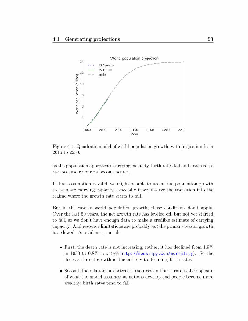
4.1 Generating projections 53
1950 2000 2050 2100 2150 2200 2250Year
4
6
8
10
12
14
Wor
ld p
opul
atio
n (b
illio
n)
World population projection
US CensusUN DESAmodel
Figure 4.1: Quadratic model of world population growth, with projection from2016 to 2250.
as the population approaches carrying capacity, birth rates fall and death rates
rise because resources become scarce.
If that assumption is valid, we might be able to use actual population growth
to estimate carrying capacity, especially if we observe the transition into the
regime where the growth rate starts to fall.
But in the case of world population growth, those conditions don’t apply.
Over the last 50 years, the net growth rate has leveled off, but not yet started
to fall, so we don’t have enough data to make a credible estimate of carrying
capacity. And resource limitations are probably not the primary reason growth
has slowed. As evidence, consider:
� First, the death rate is not increasing; rather, it has declined from 1.9%
in 1950 to 0.8% now (see http://modsimpy.com/mortality). So the
decrease in net growth is due entirely to declining birth rates.
� Second, the relationship between resources and birth rate is the opposite
of what the model assumes; as nations develop and people become more
wealthy, birth rates tend to fall.

54 Chapter 4 Prediction
We should not take too seriously the idea that this model can estimate carrying
capacity. But the predictions of a model can be credible even if the assump-
tions of the model are not strictly true. For example, population growth might
behave as if it is resource limited, even if the actual mechanism is something
else.
In fact, demographers who study population growth often use models similar
to ours. In the next section, we’ll compare our projections to theirs.
4.2 Comparing projections
Table 3 from http://modsimpy.com/worldpop contains projections from the
U.S. Census and the United Nations DESA:
table3 = tables[3]
For some years, one agency or the other has not published a projection, so
some elements of table3 contain the special value NaN, which stands for “not
a number”. NaN is often used to indicate missing data.
Pandas provides functions that deal with missing data, including dropna,
which removes any elements in a series that contain NaN. Using dropna, we
can plot the projections like this:
def plot_projections(table):
census = table.census / 1e9
un = table.un / 1e9
plot(census.dropna(), ':',
color='darkblue', label='US Census')
plot(un.dropna(), '--',
color='green', label='UN DESA')
We can run our model over the same interval:
system.t_end = 2100
run_simulation(system, update_func2)

4.3 Recurrence relations 55
1960 1980 2000 2020 2040 2060 2080 2100Year
4
6
8
10
12
Wor
ld p
opul
atio
n (b
illio
n)
World population projections
US CensusUN DESAmodel
Figure 4.2: Projections of world population generated by the U.S. CensusBureau, the United Nations, and our quadratic model.
And compare our projections to theirs. Figure 4.2 shows the results. Real
demographers expect world population to grow more slowly than our model
projects, probably because their models are broken down by region and coun-
try, where conditions are different, and they take into account expected eco-
nomic development.
Nevertheless, their projections are qualitatively similar to ours, and theirs
differ from each other almost as much as they differ from ours. So the results
from this model, simple as it is, are not entirely crazy.
4.3 Recurrence relations
The population models in the previous chapter and this one are simple enough
that we didn’t really need to run simulations. We could have solved them
mathematically. For example, we wrote the constant growth model like this:
model[t+1] = model[t] + annual_growth

56 Chapter 4 Prediction
In mathematical notation, we would write the same model like this:
xn+1 = xn + c
where xn is the population during year n, x0 is a given initial population,
and c is constant annual growth. This way of representing the model is a
recurrence relation; see http://modsimpy.com/recur.
Often it is possible to solve a recurrence relation by writing an equation that
computes xn, for a given value of n, directly; that is, without computing the
intervening values from x1 through xn−1.
In the case of constant growth we can see that x1 = x0 + c, and x2 = x1 + c.
Combining these, we get x2 = x0 + 2c, then x3 = x0 + 3c, and it is not hard
to conclude that in general
xn = x0 + nc
So if we want to know x100 and we don’t care about the other values, we can
compute it with one multiplication and one addition.
We can also write the proportional model as a recurrence relation:
xn+1 = xn + αxn
Or more conventionally as:
xn+1 = xn(1 + α)
Now we can see that x1 = x0(1 + α), and x2 = x0(1 + α)2, and in general
xn = x0(1 + α)n
This result is a geometric progression; see http://modsimpy.com/geom.
When α is positive, the factor 1 + α is greater than 1, so the elements of the
sequence grow without bound.
Finally, we can write the quadratic model like this:
xn+1 = xn + αxn + βx2n

4.4 Differential equations 57
or with the more conventional parameterization like this:
xn+1 = xn + rxn(1− xn/K)
There is no analytic solution to this equation, but we can approximate it with a
differential equation and solve that, which is what we’ll do in the next section.
4.4 Differential equations
Starting again with the constant growth model
xn+1 = xn + c
If we define ∆x to be the change in x from one time step to the next, we can
write:
∆x = xn+1 − xn = c
If we define ∆t to be the time step, which is one year in the example, we can
write the rate of change per unit of time like this:
∆x
∆t= c
This model is discrete, which means it is only defined at integer values of n
and not in between. But in reality, people are born and die all the time, not
once a year, so a continuous model might be more realistic.
We can make this model continuous by writing the rate of change in the form
of a derivative:dx
dt= c
This way of representing the model is a differential equation; see http:
//modsimpy.com/diffeq.
We can solve this differential equation if we multiply both sides by dt:
dx = cdt
And then integrate both sides:
x(t) = ct+ x0

58 Chapter 4 Prediction
Similarly, we can write the proportional growth model like this:
∆x
∆t= αx
And as a differential equation like this:
dx
dt= αx
If we multiply both sides by dt and divide by x, we get
1
xdx = α dt
Now we integrate both sides, yielding:
lnx = αt+K
where ln is the natural logarithm and K is the constant of integration. Expo-
nentiating both sides1, we have
exp(log(x)) = x = exp(αt+K)
which we can rewrite
x = exp(αt) exp(K)
Since K is an arbitrary constant, exp(K) is also an arbitrary constant, so we
can write
x = C exp(αt)
where C = exp(K). There are many solutions to this differential equation,
with different values of C. The particular solution we want is the one that
has the value x0 when t = 0. Well, when t = 0, x(t) = C, so C = x0 and the
solution we want is
x(t) = x0 exp(αt)
If you would like to see this derivation done more carefully, you might like this
video: http://modsimpy.com/khan1.
1The exponential function can be written exp(x) or ex. In this book I use the first formbecause it resembles the Python code.

4.5 Analysis and simulation 59
4.5 Analysis and simulation
Once you have designed a model, there are generally two ways to proceed:
simulation and analysis. Simulation often comes in the form of a computer
program that models changes in a system over time, like births and deaths, or
bikes moving from place to place. Analysis often comes in the form of algebra;
that is, symbolic manipulation using mathematical notation.
Analysis and simulation have different capabilities and limitations. Simulation
is generally more versatile; it is easy to add and remove parts of a program
and test many versions of a model, as we have done in the previous examples.
But there are several things we can do with analysis that are harder or impos-
sible with simulations:
� With analysis we can sometimes compute, exactly and efficiently, a value
that we could only approximate, less efficiently, with simulation. For
example, in Figure 3.5, we can see that net growth goes to zero near 14
billion, and we could estimate carrying capacity using a numerical search
algorithm (more about that later). But with the analysis in Section 3.9,
we get the general result that K = −α/β.
� Analysis often provides “computational shortcuts”, that is, the ability
to jump forward in time to compute the state of a system many time
steps in the future without computing the intervening states.
� We can use analysis to state and prove generalizations about models;
for example, we might prove that certain results will always or never
occur. With simulations, we can show examples and sometimes find
counterexamples, but it is hard to write proofs.
� Analysis can provide insight into models and the systems they describe;
for example, sometimes we can identify regimes of qualitatively different
behavior and key parameters that control those behaviors.
When people see what analysis can do, they sometimes get drunk with power,
and imagine that it gives them a special ability to see past the veil of the
material world and discern the laws of mathematics that govern the universe.
When they analyze a model of a physical system, they talk about “the math

60 Chapter 4 Prediction
behind it” as if our world is the mere shadow of a world of ideal mathematical
entities2.
This is, of course, nonsense. Mathematical notation is a language designed
by humans for a purpose, specifically to facilitate symbolic manipulations like
algebra. Similarly, programming languages are designed for a purpose, specif-
ically to represent computational ideas and run programs.
Each of these languages is good for the purposes it was designed for and less
good for other purposes. But they are often complementary, and one of the
goals of this book is to show how they can be used together.
4.6 Analysis with WolframAlpha
Until recently, most analysis was done by rubbing graphite on wood pulp3,
a process that is laborious and error-prone. A useful alternative is symbolic
computation. If you have used services like WolframAlpha, you have used
symbolic computation.
For example, if you go to https://www.wolframalpha.com/ and type
df(t) / dt = alpha f(t)
WolframAlpha infers that f(t) is a function of t and alpha is a parameter; it
classifies the query as a “first-order linear ordinary differential equation”, and
reports the general solution:
f(t) = c1 exp(αt)
If you add a second equation to specify the initial condition:
df(t) / dt = alpha f(t), f(0) = p0
WolframAlpha reports the particular solution:
2I am not making this up; see http://modsimpy.com/plato.3Or “rubbing the white rock on the black rock”, a line I got from Woodie Flowers, who
got it from Stephen Jacobsen.

4.7 Analysis with SymPy 61
f(t) = p0 exp(αt)
WolframAlpha is based on Mathematica, a powerful programming language
designed specifically for symbolic computation.
4.7 Analysis with SymPy
Python has a library called SymPy that provides symbolic computation tools
similar to Mathematica. They are not as easy to use as WolframAlpha, but
they have some other advantages.
Before we can use SymPy, we have to import it:
from sympy import *
SymPy defines many functions, and some of them conflict with functions de-
fined in modsim and the other libraries we’re using, I suggest that you do
symbolic computation with SymPy in a separate notebook.
The code for this section and the next is in this notebook: http://modsimpy.
com/sympy04.
SymPy defines a Symbol object that represents symbolic variable names, func-
tions, and other mathematical entities. object
SymPy provides a function called symbols that takes a string and returns a
Symbol object. So if we run this assignment:
t = symbols('t')
Python understands that t is a symbol, not a numerical value. If we now run
expr = t + 1
Python doesn’t try to perform numerical addition; rather, it creates a new
Symbol that represents the sum of t and 1. We can evaluate the sum using

62 Chapter 4 Prediction
subs, which substitutes a value for a symbol. This example substitutes 2 for
t:
expr.subs(t, 2)
The result is 3. Functions in SymPy are represented by a special kind of
Symbol:
f = Function('f')
Now if we write f(t), we get an object that represents the evaluation of a
function, f , at a value, t. But again SymPy doesn’t actually try to evaluate
it.
4.8 Differential equations in SymPy
SymPy provides a function, diff, that can differentiate a function. We can
apply it to f(t) like this:
dfdt = diff(f(t), t)
The result is a Symbol that represents the derivative of f with respect to t.
But again, SymPy doesn’t try to compute the derivative yet.
To represent a differential equation, we use Eq:
alpha = symbols('alpha')
eq1 = Eq(dfdt, alpha*f(t))
The result is an object that represents an equation, which is displayed like
this:d
dtf(t) = αf(t)
Now we can use dsolve to solve this differential equation:
solution_eq = dsolve(eq1)

4.9 Solving the quadratic growth model 63
The result is the equation
f(t) = C1 exp(αt)
This is the general solution, which still contains an unspecified constant,
C1. To get the particular solution where f(0) = p0, we substitute p0 for C1.
First, we have to create two more symbols:
C1, p0 = symbols('C1 p0')
Now we can perform the substitution:
particular = solution_eq.subs(C1, p0)
The result is
f(t) = p0 exp(αt)
This function is called the exponential growth curve; see http://modsimpy.
com/expo.
4.9 Solving the quadratic growth model
In the notebook for this chapter, you will see how to use the same tools to solve
the quadratic growth model with parameters r and K. The general solution
is
f(t) =K exp(C1K + rt)
exp(C1K + rt)− 1
To get the particular solution where f(0) = p0, we evaluate the general solution
at t = 0, which yields:
f(0) =K exp(C1K)
exp(C1K)− 1
Then we set this expression equal to p0 and solve for C1. The result is:
C1 =1
Klog
(− p0K − p0
)Finally, we substitute this value of C1 into the general solution, which yields:
f(t) =Kp0 exp(rt)
K + p0 exp(rt)− p0

64 Chapter 4 Prediction
This function is called the logistic growth curve; see http://modsimpy.
com/logistic. In the context of growth models, the logistic function is often
written, equivalently,
f(t) =K
1 + A exp(−rt)where A = (K − p0)/p0.
If you would like to see this differential equation solved by hand, you might
like this video: http://modsimpy.com/khan2
4.10 Summary
The following tables summarize the results so far:
Growth type Discrete (difference equation)
Constant linear: xn = p0 + αn
Proportional geometric: xn = p0(1 + α)n
Continuous (differential equation)
Constant linear: x(t) = p0 + αt
Proportional exponential: x(t) = p0 exp(αt)
Quadratic logistic: x(t) = K/(1 + A exp(−rt))
What I’ve been calling the constant growth model is more commonly called
“linear growth” because the solution is a line. Similarly, what I’ve called
proportional is commonly called “exponential”, and what I’ve called quadratic
is commonly called “logistic”.
I avoided the more common terms until now because I thought it would be
strange to use them before we solved the equations and discovered the func-
tional form of the solutions.

4.11 DataFrames and Series 65
index
columns
census
1950
2015
2557628654...
prb un
DataFrame
name = 'census'
1950
2015
2557628654...
Series
valuesindex
Figure 4.3: The elements that make up a DataFrame and a Series.
4.11 DataFrames and Series
So far we’ve been using DataFrame and Series objects without really under-
standing how they work. In this section we’ll review what we know so far and
get into a little more detail.
Each DataFrame contains three objects: index is a sequence of labels for the
rows, columns is a sequence of labels for the columns, and values is an array
that contains the data. Figure 4.3 shows these elements graphically.
A Series also contains index and values; it does not have columns, but it
does contain name, which is a string.
To determine the type of these objects, we can use the Python function type:
type(table2)
type(table2.index)
type(table2.columns)
type(table2.values)
If table2 is a DataFrame, the type of table2.index is Int64Index, which is
a defined by Pandas. The type of table2.columns is Index. These Index
objects are similar to Series objects.

66 Chapter 4 Prediction
The type of table2.values is ndarray, which is the primary array type pro-
vided by NumPy; the name indicates that the array can have an arbitrary
number of dimensions (N-dimensional).
In a Series, the index is an Index object and the values are stores in an
ndarray. Figure 4.3 shows theses elements graphically.
In the modsim library, the functions get_first_label and get_last_label
provide a simple way to access the index of a DataFrame or Series:
def get_first_label(series):
return series.index[0]
def get_last_label(series):
return series.index[-1]
In brackets, the number 0 selects the first label; the number -1 selects the last
label.
Several of the objects defined in modsim are modified versions of Series ob-
jects. A System object is a Series where the labels are variables names; a
TimeSeries object is a Series where the labels are times.
Defining these objects wasn’t necessary; we could do all the same things using
Series objects. But giving them different names makes the code easier to
read and understand, and helps avoid certain kinds of errors (like getting two
Series objects mixed up).
If you write simulations in Python in the future, you can continue using the
objects in modsim, if you find them useful, or you can use Pandas objects
directly.
4.12 One queue or two?
This section presents an exercise where you can apply what you’ve learned
so far to a question related to queueing theory (the study of systems that
involve waiting in lines, also known as “queues”). A solution to this exercise
is in queue_soln.ipynb in the repository for this book.

4.12 One queue or two? 67
λ μ λμ
μλ
μ
μ
Figure 4.4: One queue, one server (left), one queue, two servers (middle), twoqueues, two servers (right).
Suppose you are designing the checkout area for a new store. You have enough
room for two checkout counters and a waiting area for customers. You can
make two lines, one for each counter, or one line that serves both counters.
In theory, you might expect a single line to be better, but it has some practical
drawbacks: in order to maintain a single line, you would have to install rope
barriers, and customers might be put off by what seems to be a longer line,
even if it moves faster.
So you’d like to check whether the single line is really better and by how much.
Simulation can help answer this question.
Figure 4.4 shows the three scenarios we’ll consider. As we did in the bikeshare
model, we’ll assume that a customer is equally likely to arrive during any
timestep. I’ll denote this probability using the Greek letter lambda, λ, or the
variable name lam. Since it’s a new store, we don’t know what the value of λ
will be, so we’ll have to consider a range of possibilities.
Based on data from other stores, you know that it takes 5 minutes for a
customer to check out, on average. But checkout times are highly variable:
most customers take less than 5 minutes, but some take substantially more.
A simple way to model this variability is to assume that when a customer is
checking out, they have the same probability of finishing up during each time
step. I’ll denote this probability using the Greek letter mu, µ, or the variable
name mu.
If we choose µ = 1/5, the average number of time steps for each checkout will
be 5 minutes, which is consistent with the data.
Now we’re ready to get started. I’ll make some suggestions for how to proceed.

68 Chapter 4 Prediction
As always, you should practice incremental development: write no more than
one or two lines of code a time, and test as you go!
1. Write a function called make_system that takes lam and mu as parameters
and returns a System object with variables lam, mu, x, and duration. x
is the number if customers in the system, including customers in line and
at the checkout counters; x should be initialized to 0. duration is the
number of time steps to simulate; I set it to 8 hours, in minutes. Test
this function by creating a System object with lam=1/8 and mu=1/5.
2. Write a function called run_simulation that takes a System object and
simulates the number of time steps specified by duration. Start by
simulating a single queue with a single checkout counter, which I’ll call
a “server”. During each time step, a customer can finish checking out
(but only if there is a customer in the store), and a customer can arrive.
3. In run_simulation, add a few lines of code to create a TimeSeries and
store the number of customers in the store, x, at the end of each time
step. After the simulation runs, store the TimeSeries as a new system
variable called results. Plot results and confirm that the simulation
behaves as expected.
4. To compute the average number of customers in the store, L, you can
write system.results.mean(). You can use the observed value of W
to compute the average time customers spend in the store, W , which
includes time in queue and time at the counter. L and W are related by
Little’s Law (see https://en.wikipedia.org/wiki/Little’s_law):
L = λW
Modify run_simulation to compute L and W and store them as system
variables.
5. Use linspace to create an array of values for λ, from about 10% to 90%
of µ. Write a function called sweep_lam that takes an array of values for
λ and a single value for µ. It should call runsimulation once for each
value of λ; after each simulation, it should print λ and the resulting value
of W . Then modify it to plot the results rather than printing them. Run
sweep_series with 50 to 100 values of λ to get a sense of how much the
results vary from one run to the next. What happens as λ gets close to
µ?

4.12 One queue or two? 69
6. Next, write a version of run_simulation that models the scenario with
one queue and two servers. Hint: if there are at least two customers in
the store, there are two chances for a customer to finish checking out.
Test this version with a wider range of values for λ, maybe going up to
160% of µ.
7. You might want to split run_simulation into two parts: and update_func
that takes a System object and simulates one time step, and a general
version of run_simulation that takes udpate_func as a parameter.
8. Write a third version of run_simulation, or a third update_func, that
models the scenario with two queues and two servers. You might have
to add system variables, q1 and q2, to keep track of the number of
customers in each queue. When a customer arrives, they should join
whichever line is shorter.
9. Which system yields shorter wait times, one queue or two? Since the
results of a single simulation are so variable, it might not be easy to
tell. One option is to run the simulation 50 to 100 times, with a range
of values for λ, to model days with different numbers of customers, and
compute the average of the daily averages.

70 Chapter 4 Prediction

Chapter 5
Design
In the previous chapter, we developed a model of world population growth
and used it to generate projections for the next 100 years. In this chapter, we
develop a model of an epidemic as it spreads in a susceptible population, and
use it to evaluate the effectiveness of possible interventions.
My presentation of the SIR model in this chapter, and the analysis in the next
chapter, is based on an excellent article by David Smith and Lang Moore1.
You can view the code for this chapter at http://modsimpy.com/chap05. For
instructions on downloading and running the code, see Section 0.4.
5.1 The Freshman Plague
Every year at Olin College, about 90 new students come to campus from
around the country and the world. Most of them arrive healthy and happy,
but usually at least one brings with them some kind of infectious disease. A
few weeks later, predictably, some fraction of the incoming class comes down
with what we call “The Freshman Plague”.
1Smith and Moore, “The SIR Model for Spread of Disease,” Journal of Online Mathe-matics and its Applications, December 2001, at http://modsimpy.com/sir.

72 Chapter 5 Design
In this chapter we introduce a well-known model of infectious disease, the
Kermack-McKendrick model, and use it to explain the progression of the dis-
ease over the course of the semester, predict the effect of possible interventions
(like immunization) and design the most effective intervention campaign.
So far we have done our own modeling; that is, we’ve chosen physical sys-
tems, identified factors that seem important, and made decisions about how
to represent them. In this chapter we start with an existing model and reverse-
engineer it. Along the way, we consider the modeling decisions that went into
it and identify its capabilities and limitations.
5.2 The SIR model
The Kermack-McKendrick model is a simple version of an SIR model, so-
named because it considers three categories of people:
� S: People who are “susceptible”, that is, capable of contracting the dis-
ease if they come into contact with someone who is infected.
� I: People who are “infectious”, that is, capable of passing along the
disease if they come into contact with someone susceptible.
� R: People who are “recovered”.
In the basic version of the model, people who have recovered are considered to
be immune to reinfection. That is a reasonable model for some diseases, but
not for others, so it should be on the list of assumptions to reconsider later.
Let’s think about how the number of people in each category changes over time.
Suppose we know that people with the disease are infectious for a period of
4 days, on average. If 100 people are infectious at a particular point in time,
and we ignore the particular time each one became infected, we expect about
1 out of 4 to recover on any particular day.
Putting that a different way, if the time between recoveries is 4 days, the
recovery rate is about 0.25 recoveries per day, which we’ll denote with the
Greek letter gamma, γ. If the total number of people in the population is N ,

5.3 The SIR equations 73
and the fraction currently infectious is i, the total number of recoveries we
expect per day is γiN .
Now let’s think about the number of new infections. Suppose we know that
each susceptible person comes into contact with 1 person every 3 days, on
average, in such a way that they would contract the disease if the other person
is infected. We’ll denote this contact rate with the Greek letter beta, β.
It’s probably not reasonable to assume that we know β ahead of time, but
later we’ll see how to estimate it based on data from previous outbreaks.
If s is the fraction of the population that’s susceptible, sN is the number of
susceptible people, βsN is the number of contacts per day, and βsiN is the
number of those contacts where the other person is infectious.
In summary:
� The number of recoveries we expect per day is γiN ; dividing by N yields
the fraction of the population that recovers in a day, which is γi.
� The number of new infections we expect per day is βsiN ; dividing by N
yields the fraction of the population that gets infected in a day, which is
βsi.
This model assumes that the population is closed; that is, no one arrives or
departs, so the size of the population, N , is constant.
5.3 The SIR equations
If we treat time as a continuous quantity, we can write differential equations
that describe the rates of change for s, i, and r (where r is the fraction of the
population that has recovered):
ds
dt= −βsi
di
dt= βsi− γi
dr
dt= γi

74 Chapter 5 Design
Susceptible Infectious Recovered
β γ
Figure 5.1: Stock and flow diagram for an SIR model.
To avoid cluttering the equations, I leave it implied that s is a function of
time, s(t), and likewise for i and r.
SIR models are examples of compartment models, so-called because they
divide the world into discrete categories, or compartments, and describe transi-
tions from one compartment to another. Compartments are also called stocks
and transitions between them are called flows.
In this example, there are three stocks — susceptible, infectious, and recov-
ered — and two flows — new infections and recoveries. Compartment mod-
els are often represented visually using stock-and-flow diagrams (see http:
//modsimpy.com/stock. Figure 5.1 shows the stock and flow diagram for an
SIR model.
Stocks are represented by rectangles, flows by arrows. The widget in the
middle of the arrows represents a valve that controls the rate of flow; the
diagram shows the parameters that control the valves.
5.4 Implementation
For a given physical system, there are many possible models, and for a given
model, there are many ways to represent it. For example, we can represent
an SIR model as a stock-and-flow diagram, as a set of differential equations,
or as a Python program. The process of representing a model in these forms
is called implementation. In this section, we implement the SIR model in
Python.
To get started, I’ll represent the initial state of the system using a State object,
which is defined in the modsim library. A State object is a collection of state

5.4 Implementation 75
variables; each state variable represents information about the system that
changes over time. In this example, the state variables are S, I, and R; they
represent the fraction of the population in each compartment.
Creating a State object is similar to creating a System object. We can ini-
tialize the State object with the number of people in each compartment:
init = State(S=89, I=1, R=0)
And then convert the numbers to fractions by dividing by the total:
init /= sum(init)
For now, let’s assume we know the time between contacts and time between
recoveries:
tc = 3 # time between contacts in days
tr = 4 # recovery time in days
In that case we can compute the parameters of the model:
beta = 1 / tc # contact rate in per day
gamma = 1 / tr # recovery rate in per day
Now we need a System object to store the parameters and initial conditions.
The following function takes the system parameters as function parameters
and returns a new System object:
def make_system(beta, gamma):
init = State(S=89, I=1, R=0)
init /= sum(init)
t0 = 0
t_end = 7 * 14
return System(init=init, t0=t0, t_end=t_end,
beta=beta, gamma=gamma)
The default value for t_end is 14 weeks, about the length of a semester.

76 Chapter 5 Design
5.5 The update function
At any point in time, the state of the system is represented by a State object
with three variables, S, I and R. Next we’ll define an update function that
takes the State object as a parameter, along with the System object that
contains the parameters, and computes the state of the system during the
next time step:
def update1(state, system):
s, i, r = state
infected = system.beta * i * s
recovered = system.gamma * i
s -= infected
i += infected - recovered
r += recovered
return State(S=s, I=i, R=r)
The first line uses a feature we have not seen before, multiple assignment.
The value on the right side is a State object that contains three values. The
left side is a sequence of three variable names. The assignment does just
what we want: it assigns the three values from the State object to the three
variables, in order.
The update function computes infected and recovered as a fraction of the
population, then updates s, i and r. The return value is a State that contains
the updated values.
When we call update1 like this:
state = update1(init, sir)
The result is a State object with these values:

5.6 Running the simulation 77
value
S 0.985388
I 0.011865
R 0.002747
5.6 Running the simulation
Now we can simulate the model over a sequence of time steps:
def run_simulation(system, update_func):
state = system.init
for t in linrange(system.t0, system.t_end-1):
state = update_func(state, system)
return state
The parameters of run_simulation are the System object and the update
function. The System object contains the parameters, initial conditions, and
values of t0 and t_end.
The outline of this function should look familiar; it is similar to the function
we used for the population model in Section 3.5.
We can call run_simulation like this:
system = make_system(beta, gamma)
run_simulation(system, update1)
The result is the final state of the system:
value
S 0.520819
I 0.000676
R 0.478505
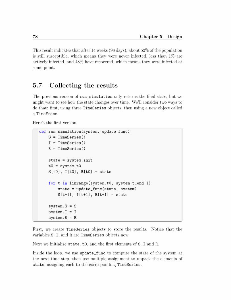
78 Chapter 5 Design
This result indicates that after 14 weeks (98 days), about 52% of the population
is still susceptible, which means they were never infected, less than 1% are
actively infected, and 48% have recovered, which means they were infected at
some point.
5.7 Collecting the results
The previous version of run_simulation only returns the final state, but we
might want to see how the state changes over time. We’ll consider two ways to
do that: first, using three TimeSeries objects, then using a new object called
a TimeFrame.
Here’s the first version:
def run_simulation(system, update_func):
S = TimeSeries()
I = TimeSeries()
R = TimeSeries()
state = system.init
t0 = system.t0
S[t0], I[t0], R[t0] = state
for t in linrange(system.t0, system.t_end-1):
state = update_func(state, system)
S[t+1], I[t+1], R[t+1] = state
system.S = S
system.I = I
system.R = R
First, we create TimeSeries objects to store the results. Notice that the
variables S, I, and R are TimeSeries objects now.
Next we initialize state, t0, and the first elements of S, I and R.
Inside the loop, we use update_func to compute the state of the system at
the next time step, then use multiple assignment to unpack the elements of
state, assigning each to the corresponding TimeSeries.

5.7 Collecting the results 79
0 20 40 60 80 100Time (days)
0.0
0.2
0.4
0.6
0.8
1.0
Fra
ctio
n of
pop
ulat
ion
SusceptibleInfectedResistant
Figure 5.2: Time series for S, I, and R over the course of 98 days.
At the end of the function, we store S, I, and R as system variables.
Now we can run the function like this:
system = make_system(beta, gamma)
run_simulation(system, update1)
We’ll use the following function to plot the results:
def plot_results(S, I, R):
plot(S, '--', color='blue', label='Susceptible')
plot(I, '-', color='red', label='Infected')
plot(R, ':', color='green', label='Resistant')
decorate(xlabel='Time (days)',
ylabel='Fraction of population')
And run it like this:
plot_results(system.S, system.I, system.R)
Figure 5.2 shows the result. Notice that it takes about three weeks (21 days)
for the outbreak to get going, and about six weeks (42 days) before it peaks.

80 Chapter 5 Design
The fraction of the population that’s infected is never very high, but it adds
up. In total, almost half the population gets sick.
5.8 Now with a TimeFrame
If the number of state variables is small, storing them as separate TimeSeries
objects might not be so bad. But a better alternative is to use a TimeFrame,
which is another object are defined in the modsim library.
A TimeFrame is almost identical to a DataFrame, which we used in Section 3.1,
with just a few changes I made to adapt it for our purposes. For more details,
you can read the modsim library source code.
Here’s a more concise version of run_simulation using a TimeFrame:
def run_simulation(system, update_func):
frame = TimeFrame(columns=system.init.index)
frame.loc[system.t0] = system.init
for t in linrange(system.t0, system.t_end-1):
frame.loc[t+1] = update_func(frame.loc[t], system)
system.results = frame
The first line creates an empty TimeFrame with one column for each state
variable. Then, before the loop starts, we store the initial conditions in the
TimeFrame at t0. Based on the way we’ve been using TimeSeries objects, it
is tempting to write:
frame[system.t0] = system.init
But when you use the bracket operator with a TimeFrame or DataFrame, it
selects a column, not a row. For example, to select a column, we could write:
frame['S']
To select a row, we have to use loc, which stands for “location”. frame.loc[0]
reads a row from a TimeFrame and

5.9 Metrics 81
frame.loc[system.t0] = system.init
assigns the values from system.init to the first row of df. Since the value on
the right side is a State, the assignment matches up the index of the State
with the columns of the TimeFrame; it assigns the S value from system.init
to the S column of the TimeFrame, and likewise with I and R.
We can use the same feature to write the loop more concisely, assigning the
State we get from update_func directly to the next row of df.
Finally, we store frame as a new system variable. We can call this version of
run_simulation like this:
run_simulation(system, update1)
And plot the results like this:
frame = system.results
plot_results(frame.S, frame.I, frame.R)
As with a DataFrame, we can use the dot operator to select columns from a
TimeFrame.
5.9 Metrics
When we plot a time series, we get a view of everything that happened when
the model ran, but often we want to boil it down to a few numbers that
summarize the outcome. These summary statistics are called metrics.
In the SIR model, we might want to know the time until the peak of the
outbreak, the number of people who are sick at the peak, the number of
students who will still be sick at the end of the semester, or the total number
of students who get sick at any point.
As an example, I will focus on the last one — the total number of sick students
— and we will consider interventions intended to minimize it.

82 Chapter 5 Design
When a person gets infected, they move from S to I, so we can get the total
number of infections by computing the difference in S at the beginning and
the end:
def calc_total_infected(system):
frame = system.results
return frame.S[system.t0] - frame.S[system.t_end]
In the notebook that accompanies this chapter, you will have a chance to write
functions that compute other metrics. Two functions you might find useful
are max and idxmax.
If you have a Series called S, you can compute the largest value of the series
like this:
largest_value = S.max()
And the label of the largest value like this:
time_of_largest_value = S.idxmax()
If the Series is a TimeSeries, the label you get from idxmax is a time or
date. You can read more about these functions in the Series documentation
at http://modsimpy.com/series.
5.10 Immunization
Models like this are useful for testing “what if?” scenarios. As an example,
we’ll consider the effect of immunization.
Suppose there is a vaccine that causes a patient to become immune to the
Freshman Plague without being infected. How might you modify the model
to capture this effect?
One option is to treat immunization as a short cut from susceptible to recov-
ered without going through infectious. We can implement this feature like
this:

5.10 Immunization 83
0 20 40 60 80 100Time (days)
0.6
0.7
0.8
0.9F
ract
ion
susc
eptib
le
No immunization10% immunization
Figure 5.3: Time series for S, with and without immunization.
def add_immunization(system, fraction):
system.init.S -= fraction
system.init.R += fraction
add_immunization moves the given fraction of the population from S to R.
If we assume that 10% of students are vaccinated at the beginning of the
semester, and the vaccine is 100% effective, we can simulate the effect like
this:
system2 = make_system(beta, gamma)
add_immunization(system2, 0.1)
run_simulation(system2, update1)
For comparison, we can run the same model without immunization and plot
the results. Figure 5.3 shows the results, plotting S as a function of time, with
and without immunization.
Without immunization, almost 47% of the population gets infected at some
point. With 10% immunization, only 31% gets infected. That’s pretty good.
So let’s see what happens if we administer more vaccines. This following
function sweeps a range of immunization rates:

84 Chapter 5 Design
def sweep_immunity(immunize_array):
sweep = SweepSeries()
for fraction in immunize_array:
sir = make_system(beta, gamma)
add_immunization(sir, fraction)
run_simulation(sir, update1)
sweep[fraction] = calc_total_infected(sir)
return sweep
The parameter of sweep_immunity is an array of immunization rates. The re-
sult is a SweepSeries object, which is defined in the modsim library. SweepSeries
is similar to TimeSeries; the difference is that the index of a SweepSeries
contains parameter values, not times.
Figure 5.4 shows a plot of the SweepSeries. Notice that the x-axis is the
immunization rate, not time.
As the immunization rate increases, the number of infections drops steeply. If
40% of the students are immunized, fewer than 4% get sick. That’s because
immunization has two effects: it protects the people who get immunized, of
course, but it also protects the rest of the population.
Reducing the number of “susceptibles” and increasing the number of “resis-
tants” makes it harder for the disease to spread, because some fraction of
contacts are wasted on people who cannot be infected. This phenomenon is
called herd immunity, and it is an important element of public health (see
http://modsimpy.com/herd).
The steepness of the curve in Figure 5.4 is a blessing and a curse. It’s a
blessing because it means we don’t have to immunize everyone, and vaccines
can protect the “herd” even if they are not 100% effective.
But it’s a curse because a small decrease in immunization can cause a big
increase in infections. In this example, if we drop from 80% immunization to
60%, that might not be too bad. But if we drop from 40% to 20%, that would
trigger a major outbreak, affecting more than 15% of the population. For a
serious disease like measles, just to name one, that would be a public health
catastrophe.

5.11 Hand washing 85
0.0 0.2 0.4 0.6 0.8 1.0Fraction immunized
0.0
0.1
0.2
0.3
0.4T
otal
frac
tion
infe
cted
Fraction infected vs. immunization rate
Figure 5.4: Fraction of the population infected as a function of immunizationrate.
One use of models like this is to demonstrate phenomena like herd immunity
and to predict the effect of interventions like vaccination. Another use is to
evaluate alternatives and guide decision making. We’ll see an example in the
next section.
5.11 Hand washing
Suppose you are the Dean of Student Affairs, and you have a budget of just
$1200 to combat the Freshman Plague. You have two options for spending
this money:
1. You can pay for vaccinations, at a rate of $100 per dose.
2. You can spend money on a campaign to remind students to wash hands
frequently.
We have already seen how we can model the effect of vaccination. Now let’s
think about the hand-washing campaign. We’ll have to answer two questions:

86 Chapter 5 Design
1. How should we incorporate the effect of hand washing in the model?
2. How should we quantify the effect of the money we spend on a hand-
washing campaign?
For the sake of simplicity, let’s assume that we have data from a similar cam-
paign at another school showing that a well-funded campaign can change stu-
dent behavior enough to reduce the infection rate by 20%.
In terms of the model, hand washing has the effect of reducing beta. That’s
not the only way we could incorporate the effect, but it seems reasonable and
it’s easy to implement.
Now we have to model the relationship between the money we spend and the
effectiveness of the campaign. Again, let’s suppose we have data from another
school that suggests:
� If we spend $500 on posters, materials, and staff time, we can change
student behavior in a way that decreases the effective value of beta by
10%.
� If we spend $1000, the total decrease in beta is almost 20%.
� Above $1000, additional spending has little additional benefit.
In the notebook for this chapter you will see how I used a logistic curve to
fit this data. The result is the following function, which takes spending as a
parameter and returns factor, which is the factor by which beta is reduced:
def compute_factor(spending):
return logistic(spending, M=500, K=0.2, B=0.01)
We use compute_factor to write add_hand_washing, which takes a System
object and a budget, and modifies system.beta to model the effect of hand
washing:
def add_hand_washing(system, spending):
factor = compute_factor(spending)
system.beta *= (1 - factor)

5.11 Hand washing 87
0 200 400 600 800 1000 1200Handwashing campaign spending (USD)
0.20
0.25
0.30
0.35
0.40
0.45
Tot
al fr
actio
n in
fect
ed
Effect of hand washing on total infections
Figure 5.5: Fraction of the population infected as a function of hand-washingcampaign spending.
Now we can sweep a range of values for spending and use the simulation to
compute the effect:
def sweep_hand_washing(spending_array):
sweep = SweepSeries()
for spending in spending_array:
sir = make_system(beta, gamma)
add_hand_washing(sir, spending)
run_simulation(sir, update1)
sweep[spending] = calc_total_infected(sir)
return sweep
Here’s how we run it:
spending_array = linspace(0, 1200, 20)
infected_sweep = sweep_hand_washing(spending_array)
88 Chapter 5 Design
Figure 5.5 shows the result. Below $200, the campaign has little effect. At
$800 it has a substantial effect, reducing total infections from 46% to 20%.
Above $800, the additional benefit is small.
5.12 Optimization
Let’s put it all together. With a fixed budget of $1200, we have to decide how
many doses of vaccine to buy and how much to spend on the hand-washing
campaign.
Here are the parameters:
num_students = 90
budget = 1200
price_per_dose = 100
max_doses = int(budget / price_per_dose)
We’ll sweep the range of possible doses:
dose_array = linrange(max_doses)
And run the simulation for each element of dose_array:
def sweep_doses(dose_array):
sweep = SweepSeries()
for doses in dose_array:
fraction = doses / num_students
spending = budget - doses * price_per_dose
sir = make_system(beta, gamma)
add_immunization(sir, fraction)
add_hand_washing(sir, spending)
run_simulation(sir, update1)
sweep[doses] = calc_total_infected(sir)
return sweep

5.12 Optimization 89
0 2 4 6 8 10 12Doses of vaccine
0.16
0.18
0.20
0.22
0.24
0.26
0.28
Tot
al fr
actio
n in
fect
ed
Total infections vs. doses
Figure 5.6: Fraction of the population infected as a function of the number ofdoses.
For each number of doses, we compute the fraction of students we can im-
munize, fraction and the remaining budget we can spend on the campaign,
spending. Then we run the simulation with those quantities and store the
number of infections.
Figure 5.6 shows the result. If we buy no doses of vaccine and spend the entire
budget on the campaign, the fraction infected is around 19%. At 4 doses, we
have $800 left for the campaign, and this is the optimal point that minimizes
the number of students who get sick.
As we increase the number of doses, we have to cut campaign spending, which
turns out to make things worse. But interestingly, when we get above 10 doses,
the effect of herd immunity starts to kick in, and the number of sick students
goes down again.
In the notebook for this chapter, you’ll have a chance to run this optimization
for a few other scenarios.

90 Chapter 5 Design
5.13 Under the hood
This chapter introduces three new objects, State, TimeFrame, and SweepSeries.
A State object is similar to a System object. The difference is that the
variables in a State object change over time; the variables in a System object
are parameters that usually don’t change. At least, they usually don’t change
during a simulation — they often vary from one simulation to the next.
In previous chapters, we used System objects to store both state variables and
parameters. Now we are using State objects to partition values that play
different roles.
A TimeFrame is a version of a Pandas DataFrame; to be honest, the biggest
difference in the name, which is intended as a reminder that the index contains
a sequence of times. Usually each row in a TimeFrame corresponds to a time
step in a simulation, and the columns correspond to the state variables.
Finally, a SweepSeries is a version of a Pandas Series where
� The index contains a range of values for a system parameter,
� And the values contain metrics that summarize the results of a simula-
tion.
In the next chapter, we’ll see a two-dimensional version of a SweepSeries,
called a SweepFrame, where the index contains one parameter, the columns
contain a second parameter, and the values contain metrics.

Chapter 6
Analysis
In the previous chapter I presented an SIR model of infectious disease, specif-
ically the Kermack-McKendrick model. We extended the model to include
vaccination and the effect of a hand-washing campaign, and used the extended
model to allocate a limited budget optimally, that is, to minimize the number
of infections.
But we assumed that the parameters of the model, contact rate and recovery
rate, were known. In this chapter, we explore the behavior of the model as we
vary these parameters, use analysis to understand these relationships better,
and propose a method for using data to estimate parameters.
You can view the code for this chapter at http://modsimpy.com/chap06. For
instructions on downloading and running the code, see Section 0.4.
6.1 Unpack
Before we analyze the SIR model, I want to make a few improvements to the
code. In the previous chapter, we used this version of run_simulation:

92 Chapter 6 Analysis
def run_simulation(system, update_func):
frame = DataFrame(columns=system.init.index)
frame.loc[system.t0] = system.init
for i in linrange(system.t0, system.t_end):
frame.loc[i+1] = update_func(frame.loc[i], system)
system.results = frame
Because we read so many variables from system, this code is a bit cluttered.
We can clean it up using unpack, which is defined in the modsim library.
unpack takes a System object as a parameter and makes the system variables
available without using the dot operator. So we can rewrite run_simulation
like this:
def run_simulation(system, update_func):
unpack(system)
frame = TimeFrame(columns=init.index)
frame.loc[t0] = init
for i in linrange(t0, t_end):
frame.loc[i+1] = update_func(frame.loc[i], system)
system.results = frame
The variables you unpack should be treated as read-only. Modifying them is
not an error, but it might not have the behavior you expect. In the notebook
for this chapter, you can use unpack to clean up update1.
6.2 Sweeping beta
Recall that β is the contact rate, which captures both the frequency of inter-
action between people and the fraction of those interactions that result in a
new infection. If N is the size of the population and s is the fraction that’s
susceptible, sN is the number of susceptibles, βsN is the number of contacts

6.2 Sweeping beta 93
per day between susceptibles and other people, and βsiN is the number of
those contacts where the other person is infectious.
As β increases, we expect the total number of infections to increase. To quan-
tify that relationship, I’ll create a range of values for β:
beta_array = linspace(0.1, 0.9, 11)
Then run the simulation for each value and print the results.
for beta in beta_array:
sir = make_system(beta, gamma)
run_simulation(sir, update1)
print(sir.beta, calc_total_infected(sir))
We can wrap that code in a function and store the results in a SweepSeries
object:
def sweep_beta(beta_array, gamma):
sweep = SweepSeries()
for beta in beta_array:
system = make_system(beta, gamma)
run_simulation(system, update1)
sweep[system.beta] = calc_total_infected(system)
return sweep
Now we can run sweep_beta like this:
infected_sweep = sweep_beta(beta_array, gamma)
And plot the results:
label = 'gamma = ' + str(gamma)
plot(infected_sweep, label=label)
The first line uses string operations to assemble a label for the plotted line:
� When the + operator is applied to strings, it joins them end-to-end, which
is called concatenation.

94 Chapter 6 Analysis
0.1 0.2 0.3 0.4 0.5 0.6 0.7 0.8 0.9Contacts per day (beta)
0.0
0.2
0.4
0.6
0.8
Fra
ctio
n in
fect
ed
gamma = 0.25
Figure 6.1: Total number of infected students as a function of the parameterbeta, with gamma = 0.25.
� The function str converts any type of object to a String representation.
In this case, gamma is a number, so we have to convert it to a string
before trying to concatenate it.
If the value of gamma is 0.25, the value of label is the string 'gamma = 0.25'.
Figure 6.1 shows the results. Remember that this figure is a parameter sweep,
not a time series, so the x-axis is the parameter beta, not time.
When beta is small, the contact rate is low and the outbreak never really takes
off; the total number of infected students is near zero. As beta increases, it
reaches a threshold near 0.3 where the fraction of infected students increases
quickly. When beta exceeds 0.5, more than 80% of the population gets sick.
6.3 Sweeping gamma
Now let’s see what that looks like for a few different values of gamma. Again,
we’ll use linspace to make an array of values:
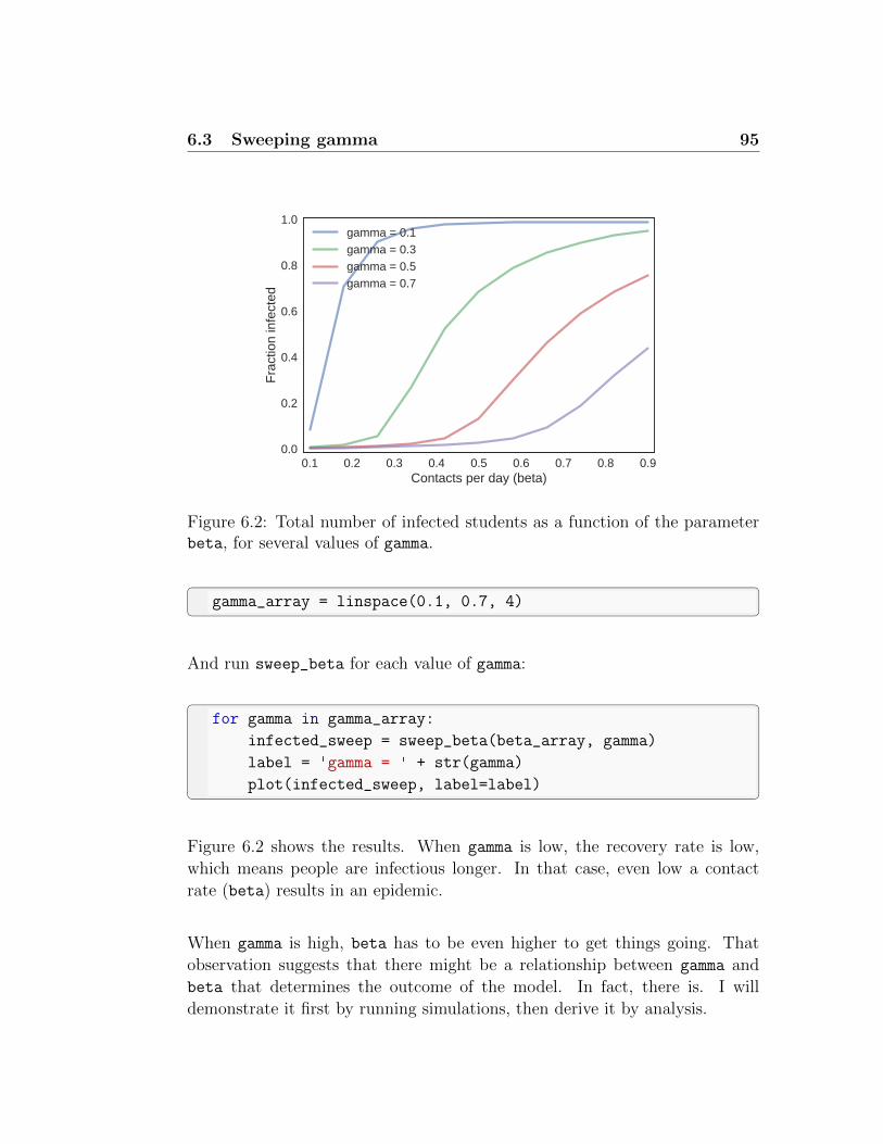
6.3 Sweeping gamma 95
0.1 0.2 0.3 0.4 0.5 0.6 0.7 0.8 0.9Contacts per day (beta)
0.0
0.2
0.4
0.6
0.8
1.0
Fra
ctio
n in
fect
ed
gamma = 0.1gamma = 0.3gamma = 0.5gamma = 0.7
Figure 6.2: Total number of infected students as a function of the parameterbeta, for several values of gamma.
gamma_array = linspace(0.1, 0.7, 4)
And run sweep_beta for each value of gamma:
for gamma in gamma_array:
infected_sweep = sweep_beta(beta_array, gamma)
label = 'gamma = ' + str(gamma)
plot(infected_sweep, label=label)
Figure 6.2 shows the results. When gamma is low, the recovery rate is low,
which means people are infectious longer. In that case, even low a contact
rate (beta) results in an epidemic.
When gamma is high, beta has to be even higher to get things going. That
observation suggests that there might be a relationship between gamma and
beta that determines the outcome of the model. In fact, there is. I will
demonstrate it first by running simulations, then derive it by analysis.
96 Chapter 6 Analysis
6.4 Nondimensionalization
Before we go on, let’s wrap the code from the previous section in a function:
def sweep_parameters(beta_array, gamma_array):
frame = SweepFrame(columns=gamma_array)
for gamma in gamma_array:
frame[gamma] = sweep_beta(beta_array, gamma)
return frame
sweep_parameters takes as parameters two arrays: a range of values for beta
and a range of values for gamma.
It creates a SweepFrame to store the results, with one column for each value
of gamma and one row for each value of beta. A SweepFrame is a kind of
DataFrame, defined in the modsim library. Its purpose is to store results from
a two-dimensional parameter sweep.
Each time through the loop, we run sweep_beta. The result is a SweepSeries
object with one element for each value of gamma. The assignment
frame[gamma] = sweep_beta(beta_array, gamma)
stores the values from the SweepSeries object as a new column in the SweepFrame,
corresponding to the current value of gamma.
At the end, the SweepFrame stores the fraction of students infected for each
pair of parameters, beta and gamma.
We can run sweep_parameters like this:
frame = sweep_parameters(beta_array, gamma_array)
Then we can loop through the results like this:
for gamma in frame.columns:
series = frame[gamma]
for beta in series.index:
frac_infected = series[beta]
print(beta, gamma, frac_infected)

6.4 Nondimensionalization 97
This is the first example we’ve seen with one for loop inside another:
� Each time the outer loop runs, it selects a value of gamma from the
columns of the DataFrame and extracts the corresponding column as a
Series.
� Each time the inner loop runs, it selects a value of beta from the Series
and selects the corresponding element, which is the fraction of student
infected.
In this example, frame has 4 columns, one for each value of gamma, and 11
rows, one for each value of beta. So these loops print 44 lines, one for each
pair of parameters.
Now let’s think about possible relationships between beta and gamma:
� When beta exceeds gamma, that means there are more contacts (that is,
potential infections) than recoveries. The difference between beta and
gamma might be called the “excess contact rate”, in units of contacts per
day.
� As an alternative, we might consider the ratio beta/gamma, which is the
number of contacts per recovery. Because the numerator and denomina-
tor are in the same units, this ratio is dimensionless, which means it
has no units.
Describing physical systems using dimensionless parameters is often a useful
move in the modeling and simulation game. It is so useful, in fact, that it has
a name: nondimensionalization (see http://modsimpy.com/nondim).
So we’ll try the second option first. In the notebook for this chapter, you can
explore the first option as an exercise.
The following function wraps the previous loops and plots the fraction infected
as a function of the ratio beta/gamma:
def plot_sweep_frame(frame):
for gamma in frame.columns:
series = frame[gamma]
for beta in series.index:
frac_infected = series[beta]
plot(beta/gamma, frac_infected, 'ro')

98 Chapter 6 Analysis
0 2 4 6 8Contact number (beta/gamma)
0.0
0.2
0.4
0.6
0.8
1.0F
ract
ion
infe
cted
Figure 6.3: Total fraction infected as a function of contact number.
Figure 6.3 shows that the results fall neatly on a single curve, at least approx-
imately. That means that we can predict the fraction of students who will be
infected based on a single parameter, the ratio beta/gamma. We don’t need to
know the values of beta and gamma separately.
6.5 Contact number
Recall that the number of new infections in a given day is βsiN , and the num-
ber of recoveries is γiN . If we divide these quantities, the result is βs/γ, which
is the number of new infections per recovery (as a fraction of the population).
When a new disease is introduced to a susceptible population, s is approxi-
mately 1, so the number of people infected by each sick person is β/γ. This
ratio is called the “contact number” or “basic reproduction number” (see
http://modsimpy.com/contact). By convention it is usually denoted R0,
but in the context of an SIR model, this notation is confusing, so we’ll use c
instead.
The results in the previous section suggest that there is a relationship be-

6.5 Contact number 99
tween c and the total number of infections. We can derive this relationship by
analyzing the differential equations from Section 5.3:
ds
dt= −βsi
di
dt= βsi− γi
dr
dt= γi
In the same way we divided the contact rate by the infection rate to get the
dimensionless quantity c, now we’ll divide di/dt by ds/dt to get a ratio of
rates:di
ds= −1 +
1
cs
Dividing one differential equation by another is not an obvious move, but in
this case it is useful because it gives us a relationship between i, s and c that
does not depend on time. We can multiply both sides of the equation by ds:
di =
(−1 +
1
cs
)ds
And then integrate both sides:
i = −s+1
clog s+ q
where q is a constant of integration. Rearranging terms yields:
q = i+ s− 1
clog s
Now let’s see if we can figure out what q is. At the beginning of an epidemic,
if the fraction infected is small and nearly everyone is susceptible, we can use
the approximations i(0) = 0 and s(0) = 1 to compute q:
q = 0 + 1 +1
clog 1
Since log 1 = 0, we get q = 1.
Now, at the end of the epidemic, let’s assume that i(∞) = 0 and s(∞) is an

100 Chapter 6 Analysis
unknown quantity s∞. Now we have:
q = 1 = 0 + s∞ −1
clog s∞
Solving for c, we get
c =log s∞s∞ − 1
If we create a range of values for s∞
s_inf_array = linspace(0.0001, 0.9999, 31)
we can compute the corresponding values of c:
c_array = log(s_inf_array) / (s_inf_array - 1)
To get the total infected, we compute the difference between s(0) and s(∞),
then store the results in a Series:
frac_infected = 1 - s_inf_array
frac_infected_series = Series(frac_infected, index=c_array)
Recall from Section ?? that a Series object contains an index and a corre-
sponding sequence of values. In this case, the index is c_array and the values
are from frac_infected.
6.6 Analysis and simulation
Now we can plot the results:
plot(frac_infected_series)
Figure 6.4 compares the analytic results from this section with the simulation
results from Section 6.4. Over most of the range they are consistent with each
other, with one discrepancy: when the contact number is less than 1, analysis
indicates there should be no infections; but in the simulations a small part of
the population is affected even when c < 1.

6.6 Analysis and simulation 101
0 2 4 6 8Contact number (c)
0.0
0.2
0.4
0.6
0.8
1.0
Fra
ctio
n in
fect
ed
SimulationAnalysis
Figure 6.4: Total fraction infected as a function of contact number, showingresults from simulation and analysis.
The reason for the discrepancy is that the simulation divides time into a dis-
crete series of days, whereas the analysis treats time as a continuous quantity.
In other words, the two methods are actually based on different models. So
which model is better?
Probably neither. When the contact number is small, the early progress of
the epidemic depends on details of the scenario. If we are lucky, the original
infected person, “patient zero”, infects no one and there is no epidemic. If we
are unlucky, patient zero might have a large number of close friends, or might
work in the dining hall (and fail to observe safe food handling procedures).
For contact numbers near or less than 1, we might need a more detailed model.
But for higher contact numbers the SIR model might be good enough.
Figure 6.4 shows that if we know the contact number, we can compute the
fraction infected. But we can also read the figure the other way; that is, at
the end of an epidemic, if we can estimate the fraction of the population that
was ever infected, we can use it to estimate the contact number.
Well, at least in theory. In practice, it might not work very well, because of
the shape of the curve. When the contact number is near 2, the curve is quite

102 Chapter 6 Analysis
steep, which means that small changes in c yield big changes in the number
of infections. If we observe that the total fraction infected is anywhere from
20% to 80%, we would conclude that c is near 2.
On the other hand, for larger contact numbers, nearly the entire population
is infected, so the curve is quite flat. In that case we would not be able to
estimate c precisely, because any value greater than 3 would yield effectively
the same results. Fortunately, this is unlikely to happen in the real world; very
few epidemics affect anything like 90% of the population.
In summary, the SIR model has limitations; nevertheless, it provides insight
into the behavior of infectious disease, especially the phenomenon of herd
resistance. As we saw in the previous chapter, if we know the parameters of
the model, we can use it to evaluate possible interventions. And as we saw in
this chapter, we might be able to use data from earlier outbreaks to estimate
the parameters.

Chapter 7
Thermal systems
So far the systems we have studied have been physical, in the sense that they
exist in the world, but they have not been physics, in the sense of what physics
classes are usually about. In this chapter, we’ll do some physics, starting with
thermal systems, that is, systems where the temperature of objects changes
as heat transfers from one to another.
You can view the code for this chapter at http://modsimpy.com/chap07. For
instructions on downloading and running the code, see Section 0.4.
7.1 The coffee cooling problem
The coffee cooling problem was discussed by Jearl Walker in Scientific Amer-
ican in 19771; since then it has become a standard example of modeling and
simulation.
Here is my version of the problem:
Suppose I stop on the way to work to pick up a cup of coffee, which
I take with milk. Assuming that I want the coffee to be as hot as
possible when I arrive at work, should I add the milk at the coffee
shop, wait until I get to work, or add the milk at some point in
between?1Walker, “The Amateur Scientist”, Scientific American, Volume 237, Issue 5, November
1977.

104 Chapter 7 Thermal systems
To help answer this question, I made a trial run with the milk and coffee in
separate containers and took some measurements:
� When served, the temperature of the coffee is 90 ◦C. The volume is
300 mL.
� The milk is at an initial temperature of 5 ◦C, and I take about 50 mL.
� The ambient temperature in my car is 22 ◦C.
� The coffee is served in a well insulated cup. When I arrive at work after
30 minutes, the temperature of the coffee has fallen to 70 ◦C.
� The milk container is not as well insulated. After 15 minutes, it warms
up to 20 ◦C, nearly the ambient temperature.
To use this data and answer the question, we have to know something about
temperature and heat, and we have to make some modeling decisions.
7.2 Temperature and heat
To understand how coffee cools (and milk warms), we need a model of temper-
ature and heat. Temperature is a property of an object or a system; in SI
units it is measured in degrees Celsius (◦C). Temperature quantifies how hot
or cold the object is, which is related to the average velocity of the particles
that make up the object.
When particles in a hot object contact particles in a cold object, the hot object
gets cooler and the cold object gets warmer, as energy is transferred from one
to the other. The transferred energy is called heat; in SI units it is measured
in joules (J).
Heat is related to temperature by the following equation (see http://modsimpy.
com/thermass):
Q = C∆T
where Q is the amount of heat transferred to an object, ∆T is resulting change
in temperature, and C is the thermal mass of the object, which quantifies

7.3 Heat transfer 105
how much energy it takes to heat or cool it. In SI units, thermal mass is
measured in joules per degree Celsius (J/◦C).
For objects made primarily from one material, thermal mass can be computed
like this:
C = mcp
where m is the mass of the object and cp is the specific heat capacity of the
material (see http://modsimpy.com/specheat).
We can use these equations to estimate the thermal mass of a cup of coffee.
The specific heat capacity of coffee is probably close to that of water, which
is 4.2 J/(g ◦C). Assuming that the density of coffee is close to that of water,
which is 1 g/mL, the mass of 300 mL of coffee is 300 g, and the thermal mass
is 1260 J/◦C.
So when a cup of coffee cools from 90 ◦C to 70 ◦C, the change in temperature,
∆T is 20 ◦C, which means that 25 200 J of heat energy was transferred from
the coffee to the surrounding environment (the cup holder and air in my car).
To give you a sense of how much energy that is, if you were able to harness
all of that heat to do work (which you cannot2), you could use it to lift a cup
of coffee from sea level to 8571 m, just shy of the height of Mount Everest,
8848 m.
Assuming that the cup has less mass than the coffee, and is made from a
material with lower a specific heat, we can ignore the thermal mass of the cup.
7.3 Heat transfer
In a situation like the coffee cooling problem, there are three ways heat trans-
fers from one object to another (see http://modsimpy.com/transfer):
� Conduction: When objects at different temperatures come into contact,
the faster-moving particles of the higher-temperature object transfer ki-
netic energy to the slower-moving particles of the lower-temperature ob-
ject.
2See http://modsimpy.com/thermo.

106 Chapter 7 Thermal systems
� Convection: When particles in a gas or liquid flow from place to place,
they carry heat energy with them. Fluid flows can be caused by external
action, like stirring, or by internal differences in temperature. For exam-
ple, you might have heard that hot air rises, which is a form of “natural
convection”.
� Radiation: As the particles in an object move due to thermal energy,
they emit electromagnetic radiation. The energy carried by this radiation
depends on the object’s temperature and surface properties (see http:
//modsimpy.com/thermrad).
For objects like coffee in a car, thermal radiation is much smaller than heat
transfer due to conduction and convection, so we will ignore it.
Convection can be a complex topic, since it often depends on details of fluid
flow in three dimensions. But for this problem we will be able to get away
with a simple model called “Newton’s law of cooling”.
7.4 Newton’s law of cooling
Newton’s law of cooling asserts that the temperature rate of change for an
object is proportional to the difference in temperature between the object and
the surrounding environment:
dT
dt= −r(T − Tenv)
where T , the temperature of the object, is a function of time, t; Tenv is the
temperature of the environment, and r is a constant that characterizes how
quickly heats is transferred between the system and the environment.
Newton’s so-called “law” is really a model in the sense that it is approximately
true in some conditions, only roughly true in others, and not at all true in
others.
For example, if the primary mechanism of heat transfer is conduction, New-
ton’s law is “true”, which is to say that r is constant over a wide range of
temperatures. And sometimes we can estimate r based on the material prop-
erties and shape of the object.

7.5 Implementation 107
When convection contributes a non-negligible fraction of heat transfer, r de-
pends on temperature, but Newton’s law is often accurate enough, at least
over a narrow range of temperatures. In this case r usually has to be esti-
mated experimentally, since it depends on details of surface shape, air flow,
evaporation, etc.
When radiation makes up a substantial part of heat transfer, Newton’s law is
not a good model at all. This is the case for objects in space or in a vacuum,
and for objects at high temperatures (more than a few hundred degrees Celsius,
say).
However, for a situation like the coffee cooling problem, we expect Newton’s
model to be quite good.
7.5 Implementation
To get started, let’s forget about the milk temporarily and focus on the coffee.
I’ll create a State object to represent the initial temperature:
init = State(temp=90)
And a System object to contain the parameters of the system:
coffee = System(init=init, T_env=22, r=0.01,
t0=0, t_end=30, dt=1)
The values of T_env, t0, and t_end come from the statement of the problem.
I chose the value of r arbitrarily for now; we will figure out how to estimate it
soon.
dt is the time step we use to simulate the cooling process. Strictly speaking,
Newton’s law is a differential equation, but over a short period of time we can
approximate it with a difference equation:
∆T = −r(T − Tenv)∆t
where ∆t is a small time step and ∆T is the change in temperature during
that time step.

108 Chapter 7 Thermal systems
Note: I use ∆T to denote a change in temperature over time, but in the
context of heat transfer, you might also see ∆T used to denote the difference
in temperature between an object and its environment, T −Tenv. To minimize
confusion, I avoid this second use.
Now we can write an update function:
def update(state, system):
unpack(system)
T = state.temp
T += -r * (T - T_env) * dt
return State(temp=T)
Now if we run
update(init, coffee)
we see that the temperature after one minute is 89.3 ◦C, so the temperature
drops by about 0.7 ◦C/min, at least for this value of r.
Now we can use run_simulation, as defined in Section 5.8, to simulate a series
of time steps from t0 to t_end:
def run_simulation(system, update_func):
unpack(system)
frame = TimeFrame(columns=init.index)
frame.loc[t0] = init
ts = linrange(t0, t_end-dt, dt)
for t in ts:
frame.loc[t+dt] = update_func(frame.loc[t], system)
system.results = frame
and run it like this:

7.6 Using fsolve 109
run_simulation(coffee, update)
The result is a TimeFrame object with one row per time step and just one
column, temp. The temperature after 30 minutes is 72.3 ◦C, which is a little
higher than stated in the problem, 70 ◦C. We could adjust r by hand and find
the right value by trial and error, but we can do better, as we’ll see in the next
section.
First I want to wrap what we have so far in a function:
def make_system(T_init=90, r=0.01, volume=300, t_end=30):
init = State(temp=T_init)
system = System(init=init,
volume=volume,
r=r,
T_env=22,
t0=0,
t_end=t_end,
dt=1)
return system
make_system takes the system parameters and packs them into a System ob-
ject. Now we can simulate the coffee like this:
coffee = make_system()
run_simulation(coffee, update)
Now let’s see a better was to estimate r.
7.6 Using fsolve
SciPy provides a method called fsolve that finds the roots of non-linear equa-
tions. As a simple example, suppose you want to find the roots of the polyno-
mial
f(x) = (x− 1)(x− 2)(x− 3)

110 Chapter 7 Thermal systems
where root means a value of x that makes f(x) = 0. Because of the way I
wrote the polynomial, we can see that if x = 1, the first factor is 0; if x = 2,
the second factor is 0; and if x = 3, the third factor is 0, so those are the roots.
But usually it’s not that easy. In that case fsolve can help. First, we have
to write a function that evaluates f :
def func(x):
return (x-1) * (x-2) * (x-3)
Now we call fsolve like this:
fsolve(func, x0=0)
The first argument is the function whose roots we want. The second argument,
x0, is an initial guess about where a root might be. Generally, the closer the
initial guess is to an actual root, the faster fsolve runs. In this case, with the
initial guess x0=0, the result is 1.
Often fsolve finds the root that’s closest to the initial guess. In this example,
when x0=1.9, fsolve returns 2, and when x0=2.9, fsolve returns 3. But
this behavior can be unpredictable; with x0=1.5, fsolve returns 3.
So how can we use fsolve to estimate r?
Now, we want to find the value of r that yields a final temperature of 70 ◦C.
To work with fsolve, we need a function that takes r as a parameter and
returns the difference between the final temperature and the goal:
def error_func1(r):
system = make_system(r=r)
run_simulation(system, update)
return final_temp(system) - 70
I call a function like this an “error function” because it returns the difference
between what we got and what we wanted, that is, the error. When we find
the right value of r, this error will be 0.
We can test error_func1 like this, using our initial guess for r:

7.6 Using fsolve 111
0 5 10 15 20 25 30Time (minutes)
10
20
30
40
50
60
70
80
90
Tem
pera
ture
(C
)
coffeemilk
Figure 7.1: Temperature of the coffee and milk over time.
error_func1(r=0.01)
The result is an error of 2.3 ◦C, because the final temperature with this value
of r is too high.
Now we can call fsolve like this:
solution = fsolve(error_func1, 0.01)
r_coffee = solution[0]
The return value from fsolve is an array with a single element, which is the
root fsolve found. In this example, r_coffee turns out to be about 0.012,
in units of 1/min.
As one of the exercises for this chapter, you will use the same process to
estimate r_milk.
With the correct values of r_coffee and r_milk, the simulation results should
look like Figure 7.1, which shows the temperature of the coffee and milk over
time.

112 Chapter 7 Thermal systems
7.7 Mixing liquids
When we mix two liquids, the temperature of the mixture depends on the
temperatures of the ingredients, but it might not be obvious how to compute
it.
Assuming there are no chemical reactions between the liquids that either pro-
duce or consume heat, the total thermal energy of the system is the same
before and after mixing; in other words, thermal energy is conserved.
If the temperature of the first liquid is T1, the temperature of the second
liquid is T2, and the final temperature of the mixture is T , the heat transfer
into the first liquid is C1(T − T1) and the heat transfer into the second liquid
is C2(T − T2), where C1 and C2 are the thermal masses of the liquids.
In order to conserve energy, these heat transfers must add up to 0:
C1(T − T1) + C2(T − T2) = 0
We can solve this equation for T:
T =C1T1 + C2T2C1 + C2
For the coffee cooling problem, we have the volume of each liquid; if we also
know the density, ρ, and the specific heat capacity, cp, we can compute thermal
mass:
C = ρV cp
If we assume that the density and specific heat of the milk and coffee are equal,
they drop out of the equation, and we can write:
T =V1T1 + V2T2V1 + V2
where V1 and V2 are the volumes of the liquids. As an exercise, you can look
up the density and specific heat of milk to see how good this approximation
is.
The following function takes two System objects that represent the coffee and
milk, and creates a new System to represent the mixture:

7.8 Mix first or last? 113
def mix(s1, s2):
assert s1.t_end == s2.t_end
volume = s1.volume + s2.volume
temp = (s1.volume * final_temp(s1) +
s2.volume * final_temp(s2)) / volume
mixture = make_system(T_init=temp,
volume=volume,
r=s1.r)
return mixture
The first line is an assert statement, which is a way of checking for errors. It
compares t_end for the two systems to confirm that they have been cooling
for the same time. If not, assert displays an error message and stops the
program.
The next two statements compute the total volume of the mixture and its
temperature. Fianlly, mix makes a new System object and returns it.
This function uses the value of r from s1 as the value of r for the mixture. If s1
represents the coffee, and we are adding the milk to the coffee, this is probably
a reasonable choice. On the other hand, when we increase the amount of liquid
in the coffee cup, that might change r. So this is an assumption to we might
want to revisit when.
7.8 Mix first or last?
Now we have everything we need to solve the problem. First I’ll create objects
to represent the coffee and cream, and run for 30 minutes.

114 Chapter 7 Thermal systems
coffee = make_system(T_init=90, t_end=30,
r=r_coffee, volume=300)
run_simulation(coffee, update)
milk = make_system(T_init=5, t_end=30,
r=r_milk, volume=50)
run_simulation(milk, update)
The final temperatures, before mixing, are 70 ◦C and 21.7 ◦C. Then we mix
them:
mix_last = mix(coffee, milk)
After mixing, the temperature is 63.1 ◦C, which is still warm enough to be
enjoyable. Would we do any better if we added the milk first?
To find out, I’ll create new objects for the coffee and milk:
coffee = run(T_init=90, r=r_coffee, volume=300)
milk = run(T_init=5, r=r_milk, volume=50)
Then mix them and simulate 30 minutes:
mix_first = mix(coffee, milk)
mix_first.t_end = 30
run_simulation(mix_first, update)
The final temperature is only 61.6 ◦C. So it looks like adding the milk at the
end is better, by about 1.5 ◦C. But is that the best we can do?
7.9 Optimization
Adding the milk after 30 minutes is better than adding immediately, but maybe
there’s something in between that’s even better. To find out, I’ll use the
following function, which takes t_add as a parameter:

7.9 Optimization 115
def run_and_mix(t_add, t_total=30):
coffee = make_system(T_init=90, t_end=t_add,
r=r_coffee, volume=300)
run_simulation(coffee, update)
milk = make_system(T_init=5, t_end=t_add,
r=r_milk, volume=50)
run_simulation(milk, update)
mixture = mix(coffee, milk)
mixture.t_end = t_total - t_add
run_simulation(mixture, update)
return final_temp(mixture)
When t_add=0, we add the milk immediately; when t_add=30, we add it at
the end. Now we can sweep the range of values in between:
sweep = SweepSeries()
for t_add in linrange(0, 30, 2):
temp = run_and_mix(t_add)
sweep[t_add] = temp
Figure 7.2 shows the result. Again, note that this is a parameter sweep, not a
time series. The x-axis is the time when we add the milk, not the index of a
TimeSeries.
The final temperature is maximized when t_add=30, so adding the milk at the
end is optimal.
In the notebook for this chapter you will have a chance to explore this solution
and try some variations. For example, suppose the coffee shop won’t let me
take milk in a separate container, but I keep a bottle of milk in the refrigerator
at my office. In that case is it better to add the milk at the coffee shop, or
wait until I get to the office?

116 Chapter 7 Thermal systems
0 5 10 15 20 25 30Time added (min)
61.4
61.6
61.8
62.0
62.2
62.4
62.6
62.8
63.0
Fin
al te
mpe
ratu
re (
C)
Figure 7.2: Final temperature as a function of the time the milk is added.
7.10 Analysis
Simulating Newton’s law of cooling is almost silly, because we can solve the
differential equation analytically. If
dT
dt= −r(T − Tenv)
the general solution is
T (t) = C1 exp(−rt) + Tenv
and the particular solution where T (0) = Tinit is
Tenv + (−Tenv + Tinit) exp(−rt)
You can see how I got this solution using SymPy at http://modsimpy.com/
sympy07; if you would like to see it done by hand, you can watch this video:
http://modsimpy.com/khan3.
Now we can use the observed data to estimate the parameter r. If we observe
T (tend) = Tend, we can plug tend and Tend into the particular solution and solve

7.10 Analysis 117
for r. The result is:
r =1
tendlog
(Tinit − TenvTend − Tenv
)Plugging in tend = 30 and Tend = 70 (and again with Tinit = 90 and Tenv = 22),
the estimate for r is 0.0116.
We can use the following function to compute the time series:
def run_analysis(system):
unpack(system)
T_init = init.temp
ts = linrange(t0, t_end, dt)
temp_array = T_env + (T_init - T_env) * exp(-r * ts)
temp_series = TimeSeries(temp_array, index=ts)
system.results = TimeFrame(temp_series, columns=['temp'])
This function is similar to run_simulation; it takes a System as a param-
eter, and stores a TimeFrame as a result. We can run it like this, with
r_coffee2=0.0116:
init = State(temp=90)
coffee2 = System(init=init, T_env=22, r=r_coffee2,
t0=0, t_end=30)
run_analysis(coffee2)
The final temperature is 70 ◦C, as it should be. In fact, the results are identical
to what we got by simulation, with very small differences due to round off
errors.

118 Chapter 7 Thermal systems

Chapter 8
Pharmacokinetics
Pharmacokinetics is the study of how drugs and other substances move
around the body, react, and are eliminated. In this chapter, we will implement
one of the most widely used pharmacokinetic models: the so-called minimal
model of glucose and insulin in the blood stream.
We will use this model to fit data collected from a patient, and use the param-
eters of the fitted model to quantify the patient’s ability to produce insulin
and process glucose.
My presentation in this chapter follows Bergman (2005) “Minimal Model” (ab-
stract at http://modsimpy.com/bergman, PDF at http://modsimpy.com/
minmod).
You can view the code for this chapter at http://modsimpy.com/chap08. For
instructions on downloading and running the code, see Section 0.4.
8.1 The glucose-insulin system
Glucose is a form of sugar that circulates in the blood of animals; it is used
as fuel for muscles, the brain, and other organs. The concentration of blood
sugar is controlled by the hormone system, and especially by insulin, which
is produced by the pancreas and has the effect of reducing blood sugar.

120 Chapter 8 Pharmacokinetics
In people with normal pancreatic function, the hormone system maintains
homeostasis; that is, it keeps the concentration of blood sugar in a range
that is neither too high or too low.
But if the pancreas does not produce enough insulin, or if the cells that should
respond to insulin become insensitive, blood sugar can become elevated, a
condition called hyperglycemia. Long term, severe hyperglycemia is the
defining symptom of diabetes mellitus, a serious disease that affects almost
10% of the population in the U.S. (see http://modsimpy.com/cdc).
One of the most-used tests for hyperglycemia and diabetes is the frequently
sampled intravenous glucose tolerance test (FSIGT), in which glucose is in-
jected into the blood stream of a fasting subject (someone who has not eaten
recently), and then blood samples are collected at intervals of 2–10 minutes for
3 hours. The samples are analyzed to measure the concentrations of glucose
and insulin.
By analyzing these measurements, we can estimate several parameters of the
subject’s response; the most important is a parameter denoted SI , which quan-
tifies the effect of insulin on the rate of reduction in blood sugar.
8.2 The glucose minimal model
The “minimal model” was proposed by Bergman, Ider, Bowden, and Cobelli1.
It consists of two parts: the glucose model and the insulin model. I will present
an implementation of the glucose model; in the notebook for this chapter, you
will have the chance to implement the insulin model.
The original model was developed in the 1970s; since then, many variations
and extensions have been proposed. Bergman’s comments on the development
of the model provide insight into their process:
We applied the principle of Occam’s Razor, i.e. by asking what
was the simplest model based upon known physiology that could
1Bergman RN, Ider YZ, Bowden CR, Cobelli C., “Quantitative estimation of insulinsensitivity”, Am J Physiol. 1979 Jun;236(6):E667-77. Abstract at http://modsimpy.com/
insulin.
8.2 The glucose minimal model 121
account for the insulin-glucose relationship revealed in the data.
Such a model must be simple enough to account totally for the
measured glucose (given the insulin input), yet it must be possi-
ble, using mathematical techniques, to estimate all the character-
istic parameters of the model from a single data set (thus avoiding
unverifiable assumptions).
The most useful models are the ones that achieve this balance: including
enough realism to capture the essential features of the system without too
much complexity to be practical. In this case the practical limit is the ability
to estimate the parameters of the model using data, and to interpret the
parameters meaningfully.
Bergman discusses the features he and his colleagues thought were essential:
(1) Glucose, once elevated by injection, returns to basal level due
to two effects: the effect of glucose itself to normalize its own
concentration [...] as well as the catalytic effect of insulin to allow
glucose to self-normalize (2) Also, we discovered that the effect
of insulin on net glucose disappearance must be sluggish — that
is, that insulin acts slowly because insulin must first move from
plasma to a remote compartment [...] to exert its action on glucose
disposal.
To paraphrase the second point, the effect of insulin on glucose disposal, as
seen in the data, happens more slowly than we would expect if it depended
primarily on the the concentration of insulin in the blood. Bergman’s group
hypothesized that insulin must move, relatively slowly, from the blood to a
“remote compartment” where it has its effect.
At the time, the remote compartment was a modeling abstraction that might,
or might not, reflect something physical. Later, according to Bergman, it was
“shown to be interstitial fluid”, that is, the fluid that surrounds tissue cells. In
the history of mathematical modeling, it is common for hypothetical entities,
added to models to achieve particular effects, to be found later to correspond
to physical entities.
The glucose model consists of two differential equations:
dG
dt= −k1 [G(t)−Gb]−X(t)G(t)

122 Chapter 8 Pharmacokinetics
dX
dt= k3 [I(t)− Ib]− k2X(t)
where
� G is the concentration of blood glucose as a function of time and dG/dt
is its rate of change.
� I is the concentration of insulin in the blood as a function of time, which
is taken as an input into the model, based on measurements.
� Gb is the basal concentration of blood glucose and Ib is the basal concen-
tration of blood insulin, that is, the concentrations at equilibrium. Both
are constants estimated from measurements at the beginning or end of
the test.
� X is the concentration of insulin in the tissue fluid as a function of time,
and dX/dt is its rate of change.
� k1, k2, and k3 are positive-valued parameters that control the rates of
appearance and disappearance for glucose and insulin.
We can interpret the terms in the equations one by one:
� −k1 [G(t)−Gb] is the rate of glucose disappearance due to the effect of
glucose itself. When G(t) is above basal level, Gb, this term is negative;
when G(t) is below basal level this term is positive. So in the absence of
insulin, this term tends to restore blood glucose to basal level.
� −X(t)G(t) models the interaction of glucose and insulin in tissue fluid,
so the rate increases as either X or G increases. This term does not
require a rate parameter because the units of X are unspecified; we can
consider X to be in whatever units would make the parameter of this
term 1.
� k3 [I(t)− Ib] is the rate at which insulin diffuses between blood and tissue
fluid. When I(t) is above basal level, insulin diffuses from the blood into
the tissue fluid. When I(t) is below basal level, insulin diffuses from
tissue to the blood.
� −k2X(t) is the rate of insulin disappearance in tissue fluid as it is con-
sumed or broken down.

8.3 Data 123
The initial state of the model is X(0) = Ib and G(0) = G0, where G0 is a
constant that represents the concentration of blood sugar immediately after
the injection. In theory we could estimate G0 based on measurements, but
in practice it takes time for the injected glucose to spread through the blood
volume. Since G0 is not measurable, it is treated as a free parameter of the
model, which means that we are free to choose it to fit the data.
8.3 Data
To develop and test the model, I’ll use data from Pacini and Bergman2. The
dataset is in a file in the repository for this book, which we can read into a
DataFrame:
data = pd.read_csv('glucose_insulin.csv', index_col='time')
data has two columns: glucose is the concentration of blood glucose in
mg/dL; insulin is concentration of insulin in the blood in µU/mL (a medical
“unit”, denoted U, is an amount defined by convention in context). The index
is time in min.
Figure 8.1 shows glucose and insulin concentrations over 182 min for a subject
with normal insulin production and sensitivity.
8.4 Interpolation
Before we are ready to implement the model, there’s one problem we have to
solve. In the differential equations, I is a function that can be evaluated at
any time, t. But in the DataFrame, we only have measurements at discrete
times. This is a job for interpolation!
The modsim library provides a function named interpolate, which is a wrap-
per for the SciPy function interp1d. It takes any kind of Series as a param-
eter, including TimeSeries and SweepSeries, and returns a function. That’s
right, I said it returns a function.
2“MINMOD: A computer program to calculate insulin sensitivity and pancreatic respon-sivity from the frequently sampled intravenous glucose tolerance test”, Computer Methodsand Programs in Biomedicine 23: 113-122, 1986.

124 Chapter 8 Pharmacokinetics
0 50 100 150
100
200
300m
g/dL
glucose
0 50 100 150Time (min)
50
100
U/m
L
insulin
Figure 8.1: Glucose and insulin concentrations measured by FSIGT.
So we can call interpolate like this:
I = interpolate(data.insulin)
Then we can call the new function, I, like this:
I(18)
The result is 31.66, which is a linear interpolation between the actual mea-
surements at t=16 and t=19. We can also pass an array as an argument to
I:
ts = linrange(0, 182, 2)
I(ts)
The result is an array of interpolated values for equally-spaced values of t
between 0 and 182.
interpolate can take additional arguments, which it passes along to interp1d.
You can read about these options at http://modsimpy.com/interp.

8.5 Implementation 125
8.5 Implementation
To get started, we’ll assume that the parameters of the model are known. We’ll
implement the model and use it to generate time series for G and X. Then we’ll
see how to find parameter values that generate series that best fit the data.
Taking advantage of estimates from prior work, I’ll start with these values:
k1 = 0.03
k2 = 0.02
k3 = 1e-05
G0 = 290
And I’ll use the measurements at t=0 as the basal levels:
Gb = data.glucose[0]
Ib = data.insulin[0]
Now we can create the initial state:
init = State(G=G0, X=0)
And the System object:
system = System(init=init,
k1=k1, k2=k2, k3=k3,
I=I, Gb=Gb, Ib=Ib,
t0=0, t_end=182, dt=2)
Now here’s the update function:

126 Chapter 8 Pharmacokinetics
def update_func(state, t, system):
G, X = state
unpack(system)
dGdt = -k1 * (G - Gb) - X*G
dXdt = k3 * (I(t) - Ib) - k2 * X
G += dGdt * dt
X += dXdt * dt
return State(G=G, X=X)
As usual, the update function takes a State object and a System as parame-
ters, but there’s one difference from previous examples: this update function
also takes t. That’s because this system of differential equations is time de-
pendent; that is, time appears in the right-hand side of at least one equation.
The first line of update uses multiple assignment to extract the current values
of G and X. The second line uses unpack so we can read the system variables
without using the dot operator.
Computing the derivatives dGdt and dXdt is straightforward; we just have to
translate the equations from math notation to Python.
Then, to perform the update, we multiply each derivative by the discrete time
step dt, which is 2 min in this example. The return value is a State object
with the new values of G and X.
Before running the simulation, it is always a good idea to run the update
function with the initial conditions:
update_func(init, 0, system)
If there are no errors, and the results seem reasonable, we are ready to run the
simulation. Here’s one more version of run_simulation. It is almost the same
as in Section 7.5, with one change: it passes t as an argument to update_func.

8.5 Implementation 127
0 50 100 150
100
200
300
mg/
dL
simulationglucose data
0 50 100 150Time (min)
0.000
0.002
0.004
0.006
Arb
itrar
y un
its
remote insulin
Figure 8.2: Results from simulation of the glucose minimal model.
def run_simulation(system, update_func):
unpack(system)
frame = TimeFrame(columns=init.index)
frame.loc[t0] = init
ts = linrange(t0, t_end-dt, dt)
for t in ts:
frame.loc[t+dt] = update_func(frame.loc[t], t, system)
system.results = frame
And we can run it like this:
run_simulation(system, update_func)
The results are shown in Figure 8.2. The top plot shows simulated glucose
levels from the model along with the measured data. The bottom plot shows

128 Chapter 8 Pharmacokinetics
simulated insulin levels in tissue fluid, which is in unspecified units, and not
to be confused with measured concentration of insulin in the blood.
With the parameters I chose, the model fits the data reasonably well. We can
do better, but first, I want to replace run_simulation with a better differential
equation solver.
8.6 Numerical solution of differential equations
So far we have been solving differential equations by rewriting them as differ-
ence equations. In the current example, the differential equations are:
dG
dt= −k1 [G(t)−Gb]−X(t)G(t)
dX
dt= k3 [I(t)− Ib]− k2X(t)
If we multiply both sides by dt, we have:
dG = [−k1 [G(t)−Gb]−X(t)G(t)] dt
dX = [k3 [I(t)− Ib]− k2X(t)] dt
When dt is very small, or more precisely infinitesimal, this equation is ex-
act. But in our simulations, dt is 2 min, which is small but not infinitesimal.
In effect, the simulations assume that the derivatives dG/dt and dX/dt are
constant during each 2 min time step. That’s not exactly true, but it can be
a good enough approximation.
This method, evaluating derivatives at discrete time steps and assuming that
they are constant in between, is called Euler’s method (see http://modsimpy.
com/euler).
Euler’s method is good enough for some simple problems, but there are many
better ways to solve differential equations, including an entire family of meth-
ods called linear multistep methods (see http://modsimpy.com/lmm).
Rather than implement these methods ourselves, we will use functions from
SciPy. The modsim library provides a function called run_odeint, which is a

8.6 Numerical solution of differential equations 129
wrapper for scipy.integrate.odeint. The name odeint stands for “ordi-
nary differential equation integrator”. The equations we are solving are “ordi-
nary” because all the derivatives are with respect to the same variable; in other
words, there are no partial derivatives. And the solver is called an integrator
because solving differential equations is considered a form of integration.
scipy.integrate.odeint is a wrapper for LSODA, which is from ODEPACK, a
venerable collection of ODE solvers written in Fortran (for some of the history
of ODEPACK, see http://modsimpy.com/hindmarsh).
To use odeint, we have to provide a “slope function”:
def slope_func(state, t, system):
G, X = state
unpack(system)
dGdt = -k1 * (G - Gb) - X*G
dXdt = k3 * (I(t) - Ib) - k2 * X
return dGdt, dXdt
slope_func is similar to update_func; in fact, it takes the same parameters
in the same order. But slope_func is simpler, because all we have to do is
compute the derivatives, that is, the slopes. We don’t have to do the updates;
odeint does them for us.
Before we call run_odeint, we have to create a System object:
system2 = System(init=init,
k1=k1, k2=k2, k3=k3,
I=I, Gb=Gb, Ib=Ib,
ts=data.index)
When we were using run_simulation, we created a System object with vari-
ables t0, t_end, and dt. When we use run_odeint, we don’t need those
variables, but we do have to provide ts, which is an array or Series that
contains the times where we want the solver to evaluate G and X.
Now we can call run_odeint like this:

130 Chapter 8 Pharmacokinetics
run_odeint(system2, slope_func)
Like run_simulation, run_odeint puts the results in a TimeFrame and stores
it as a system variable named results. The columns of results match the
state variables in init, G and X. The index of results matches the values
from ts; in this example, ts contains the timestamps of the measurements.
The results are similar to what we saw in Figure 8.2. The difference is about
1% on average and never more than 2%.
8.7 Least squares
So far we have been taking the parameters as given, but in general we don’t
have that luxury. Normally we are given the data and we have to search for
the parameters that yield a time series that best matches the data.
We will do that now, in two steps:
1. First we’ll define an error function that takes a set of possible parame-
ters, simulates the system with the given parameters, and computes the
errors, that is, the differences between the simulation results and the
data.
2. Then we’ll use a SciPy function, leastsq, to search for the parameters
that minimize mean squared error (MSE).
Here’s an outline of the functions we’ll use:
� The modsim library provides fit_leastsq, which takes a function called
error_func as a parameter. It does some error-checking, then calls
scipy.optimize.leastsq, which does the real work.
� scipy.optimize.leastsq uses functions called lmdif and lmdir, which
implement the Levenberg-Marquardt algorithm for non-linear least squares
problems (see http://modsimpy.com/levmarq). These functions are
provided by another venerable FORTRAN library called MINPACK (see
http://modsimpy.com/minpack).

8.7 Least squares 131
� When scipy.optimize.leastsq runs, it calls error_func many times,
each time with a different set of parameters, until it converges on the set
of parameters that minimizes MSE.
Each time the error function runs, it creates a System object with the given
parameters, so let’s wrap that operation in a function:
def make_system(G0, k1, k2, k3, data):
init = State(G=G0, X=0)
system = System(init=init,
k1=k1, k2=k2, k3=k3,
Gb=Gb, Ib=Ib,
I=interpolate(data.insulin),
ts=data.index)
return system
make_system takes G0 and the rate constants as parameters, as well as data,
which is the DataFrame containing the measurements. It creates and returns
a System object.
Now here’s the error function:
def error_func(params, data):
system = make_system(*params, data)
run_odeint(system, slope_func)
error = system.results.G - data.glucose
return error
The parameters of error_func are
� params, which is a sequence of four system parameters, and
� data, which is the DataFrame containing the measurements.
error_func uses make_system to create the System object. This line demon-
strates a feature we have not seen before, the scatter operator, *. Applied
to params, the scatter operator unpacks the sequence, so instead of being
considered a single value, it is treated as four separate values.

132 Chapter 8 Pharmacokinetics
error_func calls run_odeint using the same slope function we saw in Sec-
tion 8.6. Then it computes the difference between the simulation results and
the data. Since system.results.G and data.glucose are both Series ob-
jects, the result of subtraction is also a Series.
Now, to do the actual minimization, we run fit_leastsq:
k1 = 0.03
k2 = 0.02
k3 = 1e-05
G0 = 290
params = G0, k1, k2, k3
best_params = fit_leastsq(error_func, params, data)
error_func is the function we just defined. params is a sequence containing
an initial guess for the four system parameters, and data is the DataFrame
containing the measurements.
Actually, the third parameter can be any object we like. fit_leastsq and
leastsq don’t do anything with this parameter except to pass it along to
error_func, so in general it contains whatever information error_func needs
to do its job.
8.8 Interpreting parameters
The return value from fit_leastsq is best_params, which we can pass along
to make_system, again using the scatter operator, and then run the simulation:
system = make_system(*best_params, data)
run_odeint(system, slope_func)
Figure 8.3 shows the results. The simulation matches the measurements well,
except during the first few minutes after the injection. But we don’t expect
the model to do well in this regime.
The reason is that the model is non-spatial; that is, it does not take into
account different concentrations in different parts of the body. Instead, it

8.8 Interpreting parameters 133
0 25 50 75 100 125 150 175Time (min)
100
150
200
250
300
350
Con
cent
ratio
n (m
g/dL
)
simulationglucose data
Figure 8.3: Simulation of the glucose minimal model with parameters thatminimize MSE.
assumes that the concentrations of glucose and insulin in blood, and insulin in
tissue fluid, are the same throughout the body. This way of representing the
body is known among experts as the “bag of blood” model.
Immediately after injection, it takes time for the injected glucose to circulate.
During that time, we don’t expect a non-spatial model to be accurate. For this
reason, we should not take the estimated value of G0 too seriously; it is useful
for fitting the model, but not meant to correspond to a physical, measurable
quantity.
On the other hand, the other parameters are meaningful; in fact, they are the
reason the model is useful. Using the best-fit parameters, we can estimate two
quantities of interest:
� “Glucose effectiveness”, E, which is the tendency of elevated glucose to
cause depletion of glucose.
� “Insulin sensitivity”, S, which is the ability of elevated blood insulin to
enhance glucose effectiveness.

134 Chapter 8 Pharmacokinetics
Glucose effectiveness is defined as the change in dG/dt as we vary G:
E ≡ −δGδG
where G is shorthand for dG/dt. Taking the derivative of dG/dt with respect
to G, we get
E = k1 +X
The glucose effectiveness index, SG, is the value of E in when blood insulin
is near its basal level, Ib. In that case, X approaches 0 and E approaches k1.
So we can use the best-fit value of k1 as an estimate of SG.
Insulin sensitivity is defined as the change in E as we vary I:
S ≡ −δEδI
The insulin sensitivity index, SI , is the value of S when E and I are at
steady state:
SI ≡δESS
δISS
E and I are at steady state when dG/dt and dX/dt are 0, but we don’t actually
have to solve those equations to find SI . If we set dX/dt = 0 and solve for X,
we find the relation:
XSS =k3k2ISS
And since E = k1 +X, we have:
SI =δESS
δISS=δXSS
δISS
Taking the derivative of XSS with respect to ISS, we have:
SI = k3/k2
So if we find parameters that make the model fit the data, we can use k3/k2as an estimate of SI .
For the example data, the estimated values of SG and SI are 0.029 and for
8.9 × 10⁻⁴. According to Pacini and Bergman, these values are within the
normal range.

8.9 The insulin minimal model 135
8.9 The insulin minimal model
Along with the glucose minimal mode, Berman et al. developed an insulin
minimal model, in which the concentration of insulin, I, is governed by this
differential equation:
dI
dt= −kI(t) + γ [G(t)−GT ] t
where
� k is a parameter that controls the rate of insulin disappearance indepen-
dent of blood glucose.
� G(t) is the measured concentration of blood glucose at time t.
� GT is the glucose threshold; when blood glucose is above this level, it
triggers an increase in blood insulin.
� γ is a parameter that controls the rate of increase (or decrease) in blood
insulin when glucose is above (or below) GT .
The initial condition is I(0) = I0. As in the glucose minimal model, we treat
the initial condition as a parameter which we’ll choose to fit the data.
The parameters of this model can be used to estimate, φ1 and φ2, which are
values that “describe the sensitivity to glucose of the first and second phase
pancreatic responsivity”. They are related to the parameters as follows:
φ1 =Imax − Ibk(G0 −Gb)
φ2 = γ × 104
where Imax is the maximum measured insulin level, and Ib and Gb are the basal
levels of insulin and glucose.
In the notebook for this chapter, you will have a chance to implement this
model, find the parameters that best fit the data, and estimate these values.

136 Chapter 8 Pharmacokinetics
Chapter 9
Projectiles
So far the differential equations we’ve worked with have been first order,
which means they involve only first derivatives. In this chapter, we turn
our attention to second order ODEs, which can involve both first and sec-
ond derivatives.
We’ll revisit the falling penny example from Chapter 1, and use odeint to
find the position and velocity of the penny as it falls, with and without air
resistance.
You can view the code for this chapter at http://modsimpy.com/chap09. For
instructions on downloading and running the code, see Section 0.4.
9.1 Newton’s second law of motion
First order ODEs can be written
dy
dx= G(x, y)
where G is some function of x and y (see http://modsimpy.com/ode). Second
order ODEs can be written
d2y
dx2= H(x, y, y′)

138 Chapter 9 Projectiles
where H is another function and y′ is shorthand for dy/dx. In particular,
we will work with one of the most famous and useful second order ODEs,
Newton’s second law of motion:
F = ma
where F is a force or the total of a set of forces, m is the mass of a moving
object, and a is its acceleration.
Newton’s law might not look like a differential equation, until we realize that
acceleration, a, is the second derivative of position, y, with respect to time, t.
With the substitution
a =d2y
dt2
Newton’s law can be written
d2y
dt2= F/m
And that’s definitely a second order ODE. In general, F can be a function of
time, position, and velocity.
Of course, this “law” is really a model, in the sense that it is a simplification
of the real world. Although it is often approximately true:
� It only applies if m is constant. If mass depends on time, position,
or velocity, we have to use a more general form of Newton’s law (see
http://modsimpy.com/varmass).
� It is not a good model for very small things, which are better described
by another model, quantum mechanics.
� And it is not a good model for things moving very fast, which are better
described by relativistic mechanics.
But for medium to large things with constant mass, moving at speeds that are
medium to slow, Newton’s model is phenomenally useful. If we can quantify
the forces that act on such an object, we can figure out how it will move.
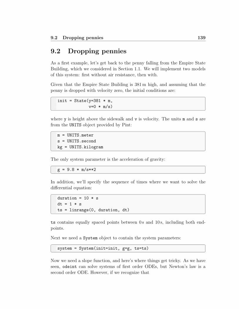
9.2 Dropping pennies 139
9.2 Dropping pennies
As a first example, let’s get back to the penny falling from the Empire State
Building, which we considered in Section 1.1. We will implement two models
of this system: first without air resistance, then with.
Given that the Empire State Building is 381 m high, and assuming that the
penny is dropped with velocity zero, the initial conditions are:
init = State(y=381 * m,
v=0 * m/s)
where y is height above the sidewalk and v is velocity. The units m and s are
from the UNITS object provided by Pint:
m = UNITS.meter
s = UNITS.second
kg = UNITS.kilogram
The only system parameter is the acceleration of gravity:
g = 9.8 * m/s**2
In addition, we’ll specify the sequence of times where we want to solve the
differential equation:
duration = 10 * s
dt = 1 * s
ts = linrange(0, duration, dt)
ts contains equally spaced points between 0 s and 10 s, including both end-
points.
Next we need a System object to contain the system parameters:
system = System(init=init, g=g, ts=ts)
Now we need a slope function, and here’s where things get tricky. As we have
seen, odeint can solve systems of first order ODEs, but Newton’s law is a
second order ODE. However, if we recognize that
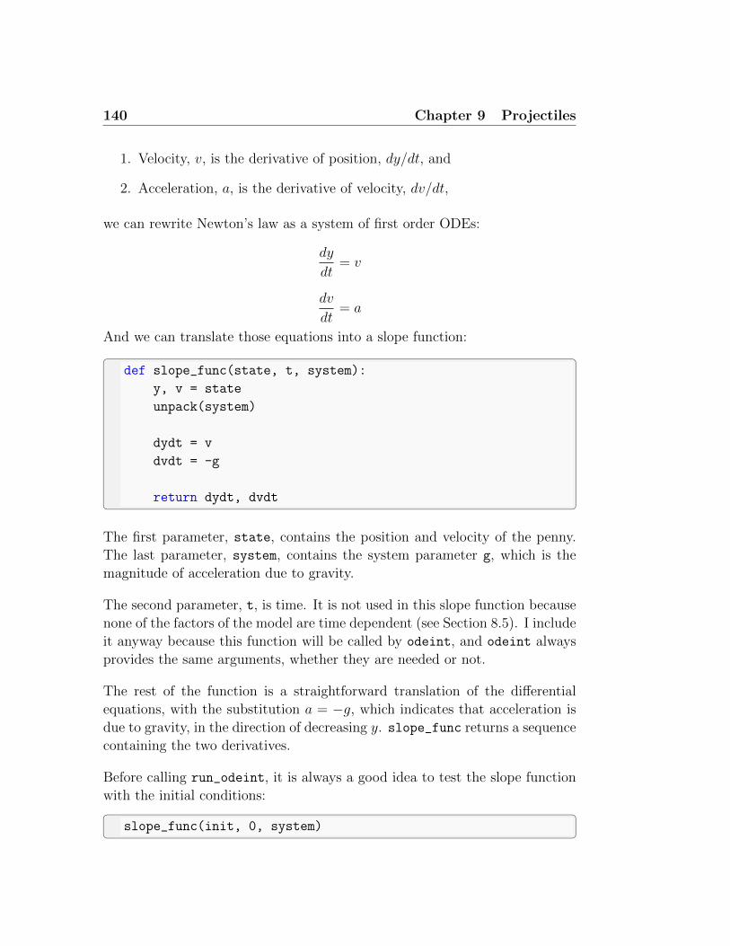
140 Chapter 9 Projectiles
1. Velocity, v, is the derivative of position, dy/dt, and
2. Acceleration, a, is the derivative of velocity, dv/dt,
we can rewrite Newton’s law as a system of first order ODEs:
dy
dt= v
dv
dt= a
And we can translate those equations into a slope function:
def slope_func(state, t, system):
y, v = state
unpack(system)
dydt = v
dvdt = -g
return dydt, dvdt
The first parameter, state, contains the position and velocity of the penny.
The last parameter, system, contains the system parameter g, which is the
magnitude of acceleration due to gravity.
The second parameter, t, is time. It is not used in this slope function because
none of the factors of the model are time dependent (see Section 8.5). I include
it anyway because this function will be called by odeint, and odeint always
provides the same arguments, whether they are needed or not.
The rest of the function is a straightforward translation of the differential
equations, with the substitution a = −g, which indicates that acceleration is
due to gravity, in the direction of decreasing y. slope_func returns a sequence
containing the two derivatives.
Before calling run_odeint, it is always a good idea to test the slope function
with the initial conditions:
slope_func(init, 0, system)

9.2 Dropping pennies 141
0 2 4 6 8 10Time (s)
100
0
100
200
300P
ositi
on (
m)
y
Figure 9.1: Height of the penny versus time, with no air resistance.
The result is a sequence containing 0 m/s for velocity and 9.8 m/s2 for accel-
eration. Now we can run odeint like this:
run_odeint(system, slope_func)
run_odeint stores the results in a TimeFrame with two columns: y contains
the height of the penny; v contains its velocity.
plot_position, which is defined in the notebook for this chapter, plots height
versus time:
plot_position(system.results)
Figure 9.1 shows the result. Since acceleration is constant, velocity increases
linearly and position decreases quadratically; as a result, the height curve is a
parabola.
In this model, height can be negative, because we have not included the effect
of the sidewalk!

142 Chapter 9 Projectiles
9.3 Onto the sidewalk
To avoid negative heights, we can use the results from the previous section
to estimate when the penny hits the sidewalk, and run the simulation for the
estimated time.
From the results, we can extract y, which is a Series that represents height
as a function of time.
y = system.results.y
To interpolate the values of y, we could use interpolate, which we saw in
Section 8.4.
Y = interpolate(y)
If we do that, we get a function that computes height as a function of time,
but that’s not what we want. Rather, we want the inverse function, time as a
function of height. The modsim library provides a function that computes it:
T = interp_inverse(y, kind='cubic')
The second parameter, kind, indicates what kind of interpolation we want:
cubic means we want a cubic spline (see http://modsimpy.com/spline).
The result is a function that maps from height to time. Now we can evaluate
the interpolating function at y=0
T_sidewalk = T(0)
The result is 8.8179 m, which agrees with the exact answer to 4 decimal places.
One caution about interpolate and interp_inverse: the function you pro-
vide has to be single valued (see http://modsimpy.com/singval).
In this example, height decreases monotonically, so for every height there is
only one corresponding time. But if we threw the penny upward and then it
fell down, the penny would pass through some heights more than once. In that
case the inverse function represented by T would not be single valued, and the
interpolation function would behave unpredictably.

9.4 With air resistance 143
9.4 With air resistance
As an object moves through a fluid, like air, the object applies force to the
air and, in accordance with Newton’s third law of motion, the air applies an
equal and opposite force to the object (see http://modsimpy.com/newton).
The direction of this drag force is opposite the direction of travel, and its
magnitude is given by the drag equation (see http://modsimpy.com/drageq):
Fd =1
2ρ v2 Cd A
where
� Fd is force due to drag, in newtons (N).
� ρ is the density of the fluid in kg/m3.
� v is velocity in m/s.
� A is the reference area of the object, in m2. In this context, the
reference area is the projected frontal area, that is, the visible area of
the object as seen from a point on its line of travel (and far away).
� Cd is the drag coefficient, a dimensionless quantity that depends on
the shape of the object (including length but not frontal area), its surface
properties, and how it interacts with the fluid.
For objects moving at moderate speeds through air, typical drag coefficients
are between 0.1 and 1.0, with blunt objects at the high end of the range and
streamlined objects at the low end (see http://modsimpy.com/dragco).
For simple geometric objects we can sometimes guess the drag coefficient with
reasonable accuracy; for more complex objects we usually have to take mea-
surements and estimate Cd from the data.
Of course, the drag equation is itself a model, based on the assumption that
Cd does not depend on the other terms in the equation: density, velocity, and
area. For objects moving in air at moderate speeds (below 45 mph or 20 m/s),
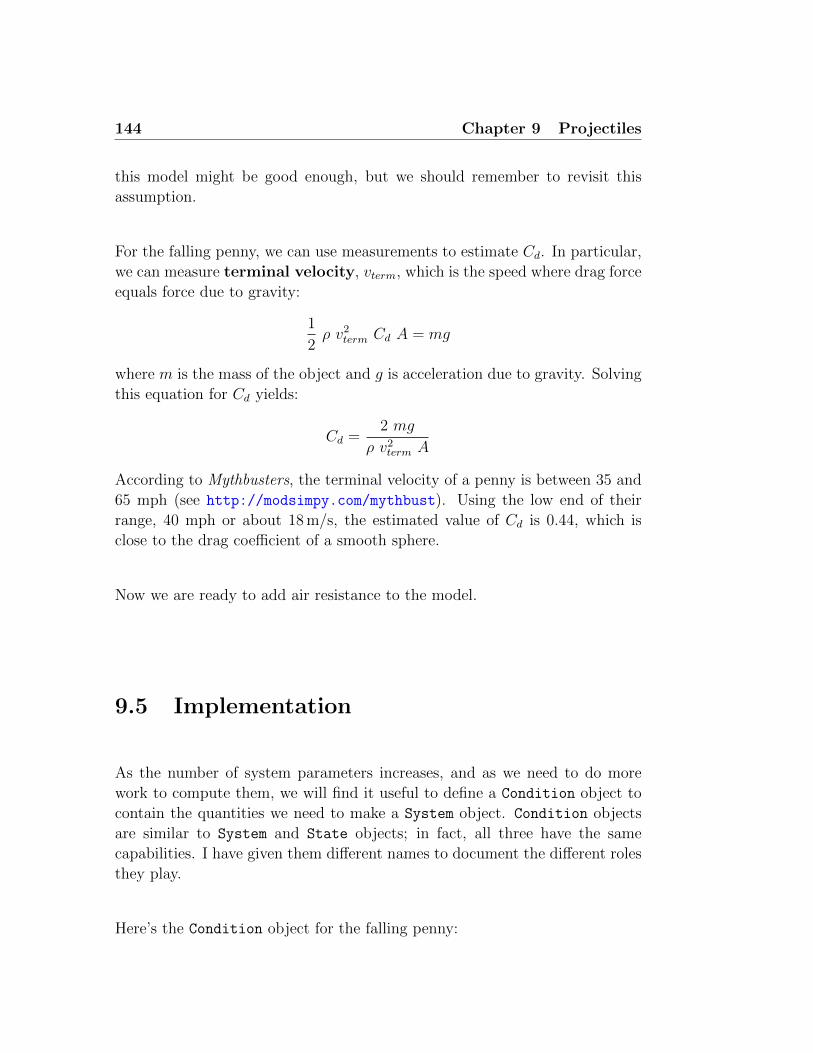
144 Chapter 9 Projectiles
this model might be good enough, but we should remember to revisit this
assumption.
For the falling penny, we can use measurements to estimate Cd. In particular,
we can measure terminal velocity, vterm, which is the speed where drag force
equals force due to gravity:
1
2ρ v2term Cd A = mg
where m is the mass of the object and g is acceleration due to gravity. Solving
this equation for Cd yields:
Cd =2 mg
ρ v2term A
According to Mythbusters, the terminal velocity of a penny is between 35 and
65 mph (see http://modsimpy.com/mythbust). Using the low end of their
range, 40 mph or about 18 m/s, the estimated value of Cd is 0.44, which is
close to the drag coefficient of a smooth sphere.
Now we are ready to add air resistance to the model.
9.5 Implementation
As the number of system parameters increases, and as we need to do more
work to compute them, we will find it useful to define a Condition object to
contain the quantities we need to make a System object. Condition objects
are similar to System and State objects; in fact, all three have the same
capabilities. I have given them different names to document the different roles
they play.
Here’s the Condition object for the falling penny:

9.5 Implementation 145
condition = Condition(height = 381 * m,
v_init = 0 * m / s,
g = 9.8 * m/s**2,
mass = 2.5e-3 * kg,
diameter = 19e-3 * m,
rho = 1.2 * kg/m**3,
v_term = 18 * m / s,
duration = 30 * s)
The mass and diameter are from http://modsimpy.com/penny. The density
of air depends on temperature, barometric pressure (which depends on alti-
tude), humidity, and composition (http://modsimpy.com/density). I chose
a value that might be typical in New York City at 20 ◦C.
Here’s a version of make_system that takes a Condition object and returns a
System:
def make_system(condition):
unpack(condition)
init = State(y=height, v=v_init)
area = np.pi * (diameter/2)**2
C_d = 2 * mass * g / (rho * area * v_term**2)
ts = linspace(0, duration, 101)
return System(init=init, g=g, mass=mass, rho=rho,
C_d=C_d, area=area, ts=ts)
It might not be obvious why we need Condition objects. One reason is to
minimize the number of variables in the System object. In this example, we
use diameter to compute area and v_term to compute C_d, but then we don’t
need diameter and v_term in the System object.
Using a Condition object is also useful because we can modify it iteratively
and create a sequence of System objects, each with a different set of conditions.
But for now, you might have to take my word that this is a good idea (see
http://modsimpy.com/zen).

146 Chapter 9 Projectiles
We can make a System like this:
system = make_system(condition)
And write a version of the slope function that includes drag:
def slope_func(state, t, system):
y, v = state
unpack(system)
f_drag = rho * v**2 * C_d * area / 2
a_drag = f_drag / mass
dydt = v
dvdt = -g + a_drag
return dydt, dvdt
f_drag is force due to drag, based on the drag equation. a_drag is acceleration
due to drag, based on Newton’s second law.
To compute total acceleration, we add accelerations due to gravity and drag,
where g is negated because it is in the direction of decreasing y, and a_drag is
positive because it is in the direction of increasing y. In the next chapter we
will use Vector objects to keep track of the direction of forces and add them
up in a less error-prone way.
After we test the slope function, we can run the simulation like this:
run_odeint(system, slope_func)
Figure 9.2 shows the result. It only takes a few seconds for the penny to
accelerate up to terminal velocity; after that, velocity is constant, so height as
a function of time is a straight line.
9.6 Dropping quarters
In the previous sections, we were given an estimate of terminal velocity, based
on measurements, and we used it to estimate the drag coefficient, Cd. Now

9.6 Dropping quarters 147
0 5 10 15 20Time (s)
0
50
100
150
200
250
300
350
Pos
ition
(m
)
y
Figure 9.2: Height of the penny versus time, with air resistance.
suppose that we are given flight time, instead. Can we use that to estimate
Cd and terminal velocity?
Suppose I drop a quarter off the Empire State Building and find that it takes
19.1 s to reach the sidewalk. Here’s a Condition object with the parameters of
a quarter (from http://modsimpy.com/quarter) and the measured duration:
condition = Condition(height = 381 * m,
v_init = 0 * m / s,
g = 9.8 * m/s**2,
mass = 5.67e-3 * kg,
diameter = 24.26e-3 * m,
rho = 1.2 * kg/m**3,
duration = 19.1 * s)
And here’s a revised version of make_system:

148 Chapter 9 Projectiles
def make_system(condition):
unpack(condition)
init = State(y=height, v=v_init)
area = np.pi * (diameter/2)**2
ts = linspace(0, duration, 101)
return System(init=init, g=g, mass=mass, rho=rho,
C_d=C_d, area=area, ts=ts)
This version does not expect the Condition object to contain v_term, but it
does expect C_d. We don’t know what C_d is, so we’ll start with an initial
guess and go from there:
condition.set(C_d=0.4)
system = make_system(condition)
run_odeint(system, slope_func)
Condition objects provide a function called set that we can use to modify
the condition variables. With C_d=0.4, the height of the quarter after 19.1 s
is −11 m. That means the quarter is moving a bit too fast, which means our
estimate for the drag coefficient is too low. We could improve the estimate by
trial and error, or we could get fsolve to do it for us.
To use fsolve, we need an error function, which we can define by encapsulating
the previous lines of code:
def height_func(C_d, condition):
condition.set(C_d=C_d)
system = make_system(condition)
run_odeint(system, slope_func)
y, v = final_state(system.results)
return y
height_func takes a hypothetical value of C_d as a parameter. It runs the
simulation with the given value of C_d and returns the final height after 19.1 s.
When we get the value of C_d right, the result should be 0, so we can use
fsolve to find it:

9.6 Dropping quarters 149
fsolve(height_func, 0.4, condition)
As we saw in Section 7.6, fsolve takes the error function and the initial guess
as parameters. Any additional parameters we give to fsolve are passed along
to height_func. In this case, we provide condition as an argument to fsolve
so we can use it inside height_func.
The result from fsolve is 0.43, which is very close to the drag coefficient we
computed for the penny, 0.44. Although it is plausible that different coins
would have similar drag coefficients, we should not take this result too seri-
ously. Remember that I chose the terminal velocity of the penny arbitrarily
from the estimated range. And I completely fabricated the flight time for the
quarter.
Nevertheless, the methods we developed for estimating C_d, based on terminal
velocity or flight time, are valid, subject to the precision of the measurements.
These methods demonstrate two ways to use models to solve problems, some-
times called forward and inverse problems. In a forward problem, you are
given the parameters of the system and asked to predict how it will behave.
In an inverse problem, you are given the behavior of the system and asked to
infer the parameters. See http://modsimpy.com/inverse.

150 Chapter 9 Projectiles

Chapter 10
Two dimensions
In the previous chapter we modeled objects moving in one dimension, with
and without drag. Now let’s move on to two dimensions, and baseball!
You can view the code for this chapter at http://modsimpy.com/chap10. For
instructions on downloading and running the code, see Section 0.4.
10.1 The Manny Ramirez problem
Manny Ramirez is a former member of the Boston Red Sox (an American
baseball team) who was notorious for a relaxed attitude and a taste for prac-
tical jokes that his managers did not always appreciate. Our objective in this
chapter is to solve the following Manny-inspired problem:
What is the minimum effort required to hit a home run in Fenway Park?
Fenway Park is a baseball stadium in Boston, Massachusetts. One of its most
famous features is the “Green Monster”, which is a wall in left field that is
unusually close to home plate, only 310 feet. To compensate for the short
distance, the wall is unusually high, at 37 feet (see http://modsimpy.com/
wally).
We want to find the minimum velocity at which a ball can leave home plate
and still go over the Green Monster. We’ll proceed in the following steps:

152 Chapter 10 Two dimensions
1. We’ll model the flight of a baseball through air.
2. For a given velocity, we’ll find the optimal launch angle, that is, the
angle the ball should leave home plate to maximize its height when it
reaches the wall.
3. Then we’ll find the minimal velocity that clears the wall, given that it
has the optimal launch angle.
As usual, we’ll have to make some modeling decisions. To get started, we’ll
ignore any spin that might be on the ball, and the resulting Magnus force (see
http://modsimpy.com/magnus).
As a result, we’ll assume that the ball travels in the plane above the left field
line, so we’ll run simulations in two dimensions, rather than three.
But we will take into account air resistance. Based on what we learned about
falling coins, it seems likely that air resistance has a substantial effect on the
flight of a baseball.
To model air resistance, we’ll need the mass, frontal area, and drag coefficient
of a baseball. Mass and diameter are easy to find (see http://modsimpy.com/
baseball). Drag coefficient is only a little harder; according to a one-pager
from NASA1, the drag coefficient of a baseball is approximately 0.3.
However, this value does depend on velocity2. At low velocities it might be as
high as 0.5, and at high velocities as low as 0.29. Furthermore, the transition
between these regimes typically happens exactly in the range of velocities we
are interested in, around 40 m/s.
To get started, I’ll assume that the drag coefficient does not depend on velocity,
but this is an issue we might want to revisit.
10.2 Vectors
Now that we are working in two dimensions, we will find it useful to work with
vector quantities, that is, quantities that represent both a magnitude and a
1“Drag on a Baseball”, available from http://modsimpy.com/nasa2Adair, The Physics of Baseball, Third Edition, Perennial, 2002

10.2 Vectors 153
direction. We will use vectors to represent positions, velocities, accelerations,
and forces in two and three dimensions.
The modsim library provides a Vector object that represents a vector quantity.
A Vector object is a like a NumPy array; it contains elements that represent
the components of the vector. For example, in a Vector that represents
a position in space, the components are the x and y coordinates (and a z
coordinate in 3-D). A Vector object also has units, like the quantities we’ve
seen in previous chapters.
You can create a Vector by specifying its components. The following Vector
represents a point 3 m to the right (or east) and 4 m up (or north) from an
implicit origin:
A = Vector(3, 4) * m
You can access the components of a Vector by name, using the dot operator;
for example, A.x or A.y. You can also access them by index, using brackets,
like A[0] or A[1].
Similarly, you can get the magnitude and angle using the dot operator, A.mag
and A.angle. Magnitude is the length of the vector: if the Vector rep-
resents position, magnitude is the distance from the origin; if it represents
velocity, magnitude is speed, that is, how fast the object is moving, regardless
of direction.
The angle of a Vector is its direction, expressed as the angle in radians from
the positive x-axis. In the Cartesian plane, the angle 0 rad is due east, and
the angle π rad is due west.
Vector objects support most mathematical operations, including addition and
subtraction:
B = Vector(1, 2) * m
A + B
A - B
For the definition and graphical interpretation of these operations, see http:
//modsimpy.com/vecops.
154 Chapter 10 Two dimensions
When you add and subtract Vector objects, the modsim library uses NumPy
and Pint to check that the operands have the same number of dimensions and
units. The notebook for this chapter shows examples for working with Vector
objects.
One note on working with angles: in mathematics, we almost always represent
angle in radians, and most Python functions expect angles in radians. But
people often think more naturally in degrees. It can be awkward, and error-
prone, to use both units in the same program. Fortunately, Pint makes it
possible to represent angles using quantities with units.
As an example, I’ll get the degree unit from UNITS, and create a quantity
that represents 45 degrees:
degree = UNITS.degree
angle = 45 * degree
Then if we need to convert to radians we can use the to function
radian = UNITS.radian
rads = angle.to(radian)
Alternatively, if we know that a quantity is represented in degrees, we can
use np.deg2rad to convert to radians. However, unlike the to function,
np.deg2rad does no error checking!
If you are given an angle and velocity, you can make a Vector by converting to
Cartesian coordinates using pol2cart. To demonstrate, I’ll extract the angle
and magnitude of A:
mag = A.mag
angle = A.angle
And then make a new Vector with the same components:
x, y = pol2cart(angle, mag)
Vector(x, y)
10.3 Modeling baseball flight 155
10.3 Modeling baseball flight
Now we’re ready to simulate the flight of the baseball. As in Section 9.5, I’ll
create a Condition object that contains the parameters of the system:
condition = Condition(x = 0 * m,
y = 1 * m,
g = 9.8 * m/s**2,
mass = 145e-3 * kg,
diameter = 73e-3 * m,
rho = 1.2 * kg/m**3,
C_d = 0.3,
angle = 45 * degree,
velocity = 40 * m / s,
duration = 5.1 * s)
Using the center of home plate as the origin, the initial height is about 1 m. The
initial velocity is 40 m/s at a launch angle of 45°. The mass, diameter, and drag
coefficient of the baseball are from the sources in Section 10.1. The acceleration
of gravity, g, is a well-known quantity, and the density of air, rho, is based on
a temperature of 20 ◦C at sea level (see http://modsimpy.com/tempress). I
chose the value of duration to run the simulation long enough for the ball to
land on the ground.
The following function uses the Condition object to make a System object.
Again, this two-step process reduces the number of variables in the System
object, and makes it easier to work with functions like fsolve.
def make_system(condition):
unpack(condition)
theta = np.deg2rad(angle)
vx, vy = pol2cart(theta, velocity)
init = State(x=x, y=y, vx=vx, vy=vy)
area = np.pi * (diameter/2)**2
ts = linspace(0, duration, 101)
return System(init=init, g=g, mass=mass,
area=area, rho=rho, C_d=C_d, ts=ts)
156 Chapter 10 Two dimensions
After unpacking Condition, we can access the variables it contains without
using the dot operator.
make_system uses np.deg2rad to convert angle to radians and pol2cart to
compute the x and y components of the initial velocity. Then it makes the
initial State object, computes area and ts, and creates the System object.
Now we’re ready for a slope function:
def slope_func(state, t, system):
x, y, vx, vy = state
unpack(system)
a_grav = Vector(0, -g)
v = Vector(vx, vy)
f_drag = -rho * v.mag * v * C_d * area / 2
a_drag = f_drag / mass
a = a_grav + a_drag
return v.x, v.y, a.x, a.y
As usual, the parameters of the slope function are a State object, time, and
a System object. In this example, we don’t use t, but we can’t leave it out
because when odeint calls the slope function, it always provides the same
arguments, whether they are needed or not.
The State object has four variables: x and y are the components of position;
vx and vy are the components of velocity.
The return values from the slope function are the derivatives of these compo-
nents. The derivative of position is velocity, so the first two return values are
just vx and vy, the values we extracted from the State object. The derivative
of velocity is acceleration, and that’s what we have to compute.
The total acceleration of the baseball is the sum of accelerations due to gravity
and drag. These quantities have both magnitude and direction, so we’ll use
Vector objects to represent them. Here’s how it works:

10.3 Modeling baseball flight 157
� a_grav is the Vector representation of acceleration due to gravity, with
magnitude g and direction along the negative y-axis.
� v is the Vector representation of velocity, which we create using the
components vx and vy. This representation makes it easier to compute
the drag force, which I explain in more detail below.
� f_drag is drag force, which is also a Vector quantity, with units of
kg m/s2, also known as newtons (N).
� a_drag is acceleration due to drag, which we get by dividing f_drag by
mass. The result is in units of acceleration, m/s2.
� a is total acceleration due to all forces, from which we can extract the
components a.x and a.y.
The last thing I have to explain is the vector form of the drag equation. In
Section 9.4 we saw the scalar form (a scalar is a single value, as contrasted
with a vector, which contains components):
Fd =1
2ρ v2 Cd A
This form was sufficient when v represented the magnitude of velocity and all
we wanted was the magnitude of drag force. But now v is a Vector and we
want both the magnitude and angle of drag.
We can do that by replacing v2, in the equation, with a vector that has the
opposite direction as v and magnitude v.mag**2. In math notation, we can
write
~Fd = −1
2ρ |v| ~v Cd A
Where |v| indicates the magnitude of v and the arrows on ~Fd and ~v indicate
that they are vectors. Negation reverses the direction of a vector, so ~Fd is in
the opposite direction of ~v.
Translating to Python we have:

158 Chapter 10 Two dimensions
f_drag = -rho * v.mag * v * C_d * area / 2
Using vectors to represent forces and accelerations makes the code concise,
readable, and less error-prone. In particular, when we add a_grav and a_drag,
the directions are likely to be correct, because they are encoded in the Vector
objects. And the units are certain to be correct, because otherwise Pint would
report an error.
As always, we can test the slope function by running it with the initial condi-
tions:
slope_func(system.init, 0, system)
10.4 Trajectories
Now we’re ready to run the simulation:
run_odeint(system, slope_func)
The result is a TimeFrame object with one column for each of the state vari-
ables, x, y, vx, and vy. We can extract the x and y components like this:
xs = system.results.x
ys = system.results.y
And plot them like this:
plot(xs, label='x')
plot(ys, label='y')
Figure 10.1 shows the result. As expected, the x component increases mono-
tonically, with decreasing velocity. And the y position climbs initially and
then descends, falling slightly below 0 m after 5.1 s.
Another way to view the same data is to plot the x component on the x-axis
and the y component on the y-axis, so the plotted line follows the trajectory
of the ball through the plane:

10.4 Trajectories 159
0 1 2 3 4 5Time (s)
0
20
40
60
80
100
Pos
ition
(m
)
xy
Figure 10.1: Simulated baseball flight, x and y components of position as afunction of time.
plot(xs, ys, label='trajectory')
Figure 10.2 shows this way of visualizing the results, which is called a trajec-
tory plot (see http://modsimpy.com/trajec).
A trajectory plot can be easier to interpret than a time series plot, because
it shows what the motion of the projectile would look like (at least from one
point of view). Both plots can be useful, but don’t get them mixed up! If you
are looking at a time series plot and interpreting it as a trajectory, you will be
very confused.
Another useful way to visualize the results is animation. You can create an-
imations using the plot function from the modsim library, with the update
argument, which tells plot that the coordinates you provide should update
the old coordinates. Here’s an example:
for x, y in zip(xs, ys):
plot(x, y, 'bo', update=True)
sleep(0.01)
This example uses two features we have not seen before:

160 Chapter 10 Two dimensions
0 20 40 60 80 100x position (m)
0
5
10
15
20
25
30
y po
sitio
n (m
)
trajectory
Figure 10.2: Simulated baseball flight, trajectory plot.
� zip takes two sequences (in this case they are Series objects) and “zips”
them together; that is, it loops through both of them at the same time,
selecting corresponding elements from each. So each time through the
loop, x and y get the next elements from xs and ys.
� sleep causes the program to pause for a given duration, in seconds.
You can see what the results look like in the notebook for this chapter.
10.5 Finding the range
Suppose we want to find the launch angle that maximizes range, that is,
the distance the ball travels in the air before landing. Assuming that the
simulation runs long enough for the ball to land, we can compute the range
like this:
1. Find the time when the height of the ball is maximized and select the
part of the trajectory where the ball is falling. We have to do this in
order to avoid problems with interpolation (see Section 9.3).

10.5 Finding the range 161
2. Then we use interpolate to find the time when the ball hits the ground,
t_land.
3. Finally, we compute the x component at t_land.
Here’s the function that does all that:
def interpolate_range(results):
xs = results.x
ys = results.y
t_peak = ys.idxmax()
descent = ys.loc[t_peak:]
T = interp_inverse(descent)
t_land = T(0)
X = interpolate(xs, kind='cubic')
return X(t_land)
interpolate_range uses idxmax to find the time when the ball hits its peak
(see Section 5.9).
Then it uses ys.loc to extract only the points from t_peak to the end. The
index in brackets includes a colon (:), which indicates that it is a slice index.
In general, a slice selects a range of elements from a Series, specifying the
start and end indices. For example, the following slice selects elements from
t_peak to t_land, including both:
ys.loc[t_peak:t_land]
If we omit the first index, like this:
ys.loc[:t_land]
we get everything from the beginning to t_land. If we omit the second index,
as in interpolate_range, we get everything from t_peak to the end of the
Series. For more about indexing with loc, see http://modsimpy.com/loc.

162 Chapter 10 Two dimensions
Next it uses interp_inverse, which we saw in Section 9.3, to make T, which
is an interpolation function that maps from height to time. So t_land is the
time when height is 0.
Finally, it uses interpolate to make X, which is an interpolation function
that maps from time to x component. So X(t_land) is the distance from
home plate when the ball lands.
We can call interpolate_range like this:
interpolate_range(system.results)
The result is 103 m, which is about 337 feet.
10.6 Optimization
To find the angle that optimizes range, we need a function that takes launch
angle as a parameter and returns range:
def range_func(angle, condition):
condition.set(angle=angle)
system = make_system(condition)
run_odeint(system, slope_func)
x_range = interpolate_range(system.results)
return x_range
We can call range_func directly like this:
range_func(45, condition)
And we can sweep a sequence of angles like this:
angles = linspace(30, 60, 11)
sweep = SweepSeries()
for angle in angles:
x_range = range_func(angle, condition)
print(angle, x_range)
sweep[angle] = x_range

10.6 Optimization 163
30 35 40 45 50 55 60Launch angle (degree)
92.5
95.0
97.5
100.0
102.5
105.0
107.5
110.0
Ran
ge (
m)
Figure 10.3: Distance from home plate as a function of launch angle, withfixed velocity.
Figure 10.3 shows the results. It looks like the optimal angle is between 40°and 45° (at least for this definition of “optimal”).
We can find the optimal angle more precisely and more efficiently using max_bounded,
which is a function in the modsim library that uses scipy.opimize.minimize_scalar
(see http://modsimpy.com/minimize).
Here’s how we run it:
res = max_bounded(range_func, [0, 90], condition)
The first parameter is the function we want to maximize. The second is the
range of values we want to search; in this case it’s the range of angles from 0°to 90°. The third argument is the Condition object, which gets passed along
as an argument when max_bounded calls range_func.
The result from max_bounded is an OptimizeResult object, which contains
several variables. The ones we want are x, which is the angle that yielded the
highest range, and fun, which is the value of range_func when it’s evaluated
at x, that is, range when the baseball is launched at the optimal angle.

164 Chapter 10 Two dimensions
10.7 Finishing off the problem
In the notebook for this chapter, you’ll have to chance to finish off the Manny
Ramirez problem. There are a few things you’ll have to do:
� In the previous section the “optimal” launch angle is the one that max-
imizes range, but that’s not what we want. Rather, we want the angle
that maximizes the height of the ball when it gets to the wall (310 feet
from home plate). So you’ll have to write a height function to compute
it, and then use max_bounded to find the revised optimum.
� Once you can find the optimal angle for any velocity, you have to find the
minimum velocity that gets the ball over the wall. You’ll write a function
that takes a velocity as a parameter, computes the optimal angle for that
velocity, and returns the height of the ball, at the wall, using the optimal
angle.
� Finally, you’ll use fsolve to find the velocity that makes the height, at
the wall, just barely 37 feet.
The notebook provides some additional hints, but at this point you should
have everything you need. Good luck!
If you enjoy this exercise, you might be interested in this paper: “How to
hit home runs: Optimum baseball bat swing parameters for maximum range
trajectories”, by Sawicki, Hubbard, and Stronge, at http://aapt.scitation.
org/doi/abs/10.1119/1.1604384.

Chapter 11
Rotation
In this chapter we model systems that involve rotating objects. In general,
rotation is complicated: in three dimensions, objects can rotate around three
axes; objects are often easier to spin around some axes than others; and they
may be stable when spinning around some axes but not others.
If the configuration of an object changes over time, it might become easier or
harder to spin, which explains the surprising dynamics of gymnasts, divers,
ice skaters, etc.
And when you apply a twisting force to a rotating object, the effect is often
contrary to intuition. For an example, see this video on gyroscopic precession
http://modsimpy.com/precess.
In this chapter, we will not take on the physics of rotation in all its glory.
Rather, we will focus on simple scenarios where all rotation and all twisting
forces are around a single axis. In that case, we can treat some vector quantities
as if they were scalars (in the same way that we sometimes treat velocity as a
scalar with an implicit direction).
This approach makes it possible to simulate and analyze many interesting
systems, but you will also encounter systems that would be better approached
with the more general toolkit.
The fundamental ideas in this chapter are angular velocity, angular accel-
eration, torque, and moment of inertia. If you are not already familiar

166 Chapter 11 Rotation
r
r dθdθ
Figure 11.1: Diagram of a roll of toilet paper, showing change in paper lengthas a result of a small rotation, dθ.
with these concepts, I will define them as we go along, and I will point to
additional reading.
As an exercise at the end of the chapter, you will use these tools to simulate
the behavior of a yo-yo (see http://modsimpy.com/yoyo). But we’ll work our
way up to it gradually, starting with toilet paper.
You can view the code for this chapter at http://modsimpy.com/chap11. For
instructions on downloading and running the code, see Section 0.4.
11.1 The physics of toilet paper
As a simple example of a system with rotation, we’ll simulate the manufacture
of a roll of toilet paper. Starting with a cardboard tube at the center, we will
roll up 47 m of paper, the typical length of a roll of toilet paper in the U.S.
(see http://modsimpy.com/paper).
Figure 11.1 shows a diagram of the system: r represents the radius of the roll
at a point in time. Initially, r is the radius of the cardboard core, Rmin. When
the roll is complete, r is Rmax.

11.2 Implementation 167
I’ll use θ to represent the total rotation of the roll in radians. In the diagram,
dθ represents a small increase in θ, which corresponds to a distance along the
circumference of the roll of r dθ.
Finally, I’ll use y to represent the total length of paper that’s been rolled.
Initially, θ = 0 and y = 0. For each small increase in θ, there is a corresponding
increase in y:
dy = r dθ
If we divide both sides by a small increase in time, dt, we get a differential
equation for y as a function of time.
dy
dt= r
dθ
dt
As we roll up the paper, r increases, too. Assuming that r increases by a fixed
amount per revolution, we can write
dr = k dθ
Where k is an unknown constant we’ll have to figure out. Again, we can divide
both sides by dt to get a differential equation in time:
dr
dt= k
dθ
dt
Finally, let’s assume that θ increases at a constant rate of 10 rad/s (about 95
revolutions per minute):dθ
dt= 10
This rate of change is called an angular velocity. Now we have a system of
three differential equations we can use to simulate the system.
11.2 Implementation
At this point we have a pretty standard process for writing simulations like
this. First, we’ll get the units we need from Pint:

168 Chapter 11 Rotation
radian = UNITS.radian
m = UNITS.meter
s = UNITS.second
And create a Condition object with the parameters of the system:
condition = Condition(Rmin = 0.02 * m,
Rmax = 0.055 * m,
L = 47 * m,
duration = 130 * s)
Rmin and Rmax are the initial and final values for the radius, r. L is the total
length of the paper, and duration is the length of the simulation in time.
Then we use the Condition object to make a System object:
def make_system(condition):
unpack(condition)
init = State(theta = 0 * radian,
y = 0 * m,
r = Rmin)
k = estimate_k(condition)
ts = linspace(0, duration, 101)
return System(init=init, k=k, ts=ts)
The initial state contains three variables, theta, y, and r.
To get started, we’ll estimate a reasonable value for k; then in Section 11.3
we’ll figure it out exactly. Here’s how we compute the estimate:
11.2 Implementation 169
def estimate_k(condition):
unpack(condition)
Ravg = (Rmax + Rmin) / 2
Cavg = 2 * pi * Ravg
revs = L / Cavg
rads = 2 * pi * revs
k = (Rmax - Rmin) / rads
return k
Ravg is the average radius, half way between Rmin and Rmax, so Cavg is the
circumference of the roll when r is Ravg.
revs is the total number of revolutions it would take to roll up length L if r
were constant at Ravg. And rads is just revs converted to radians.
Finally, k is the change in r for each radian of revolution. For these parameters,
k is about 2.8e-5 m/rad.
Now we can use the differential equations from Section 11.1 to write a slope
function:
def slope_func(state, t, system):
theta, y, r = state
unpack(system)
omega = 10 * radian / s
dydt = r * omega
drdt = k * omega
return omega, dydt, drdt
As usual, the slope function takes a State object, a time, and a System object.
The State object contains the hypothetical values of theta, y, and r at time
t. The job of the slope function is to compute the time derivatives of these
values. The time derivative of theta is angular velocity, which is often denoted
omega.
Now we can run the simulation like this:

170 Chapter 11 Rotation
0 20 40 60 80 100 1200
500
1000
Ang
le (
rad)
theta
0 20 40 60 80 100 1200
20
40
Leng
th (
m)
y
0 20 40 60 80 100 120Time(s)
20
30
40
50
Rad
ius
(mm
)
r
Figure 11.2: Results from paper rolling simulation, showing rotation, length,and radius over time.
run_odeint(system, slope_func)
Figure 11.2 shows the results. theta grows linearly over time, as we should
expect. As a result, r also grows linearly. But since the derivative of y depends
on r, and r is increasing, y grows with increasing slope.
Because this system is so simple, it is almost silly to simulate it. As we’ll
see in the next section, it is easy enough to solve the differential equations
analytically. But it is often useful to start with a simple simulation as a way
of exploring and checking assumptions.
In order to get the simulation working, we have to get the units right, which can
help catch conceptual errors early. And by plugging in realistic parameters,
we can detect errors that cause unrealistic results. For example, in this system
we can check:
� The total time for the simulation is about 2 minutes, which seems plau-
sible for the time it would take to roll 47 m of paper.
11.3 Analysis 171
� The final value of theta is about 1250 rad, which corresponds to about
200 revolutions, which also seems plausible.
� The initial and final values for r are consistent with Rmin and Rmax, as
we intended when we chose k.
But now that we have a working simulation, it is also useful to do some analysis.
11.3 Analysis
The differential equations in Section 11.1 are simple enough that we can just
solve them. Since angular velocity is constant:
dθ
dt= ω
We can find θ as a function of time by integrating both sides:
θ(t) = ωt+ C1
With the initial condition θ(0) = 0, we find C1 = 0. Similarly,
dr
dt= kω (11.1)
So
r(t) = kωt+ C2
With the initial condition r(0) = Rmin, we find C2 = Rmin. Then we can plug
the solution for r into the equation for y:
dy
dt= rω (11.2)
= [kωt+Rmin]ω
Integrating both sides yields:
y(t) =[kωt2/2 +Rmint
]ω + C3
So y is a parabola, as you might have guessed. With initial condition y(0) = 0,
we find C3 = 0.

172 Chapter 11 Rotation
We can also use these equations to find the relationship between y and r,
independent of time, which we can use to compute k. Using a move we saw in
Section 6.5, I’ll divide Equations 11.1 and 11.2, yielding
dr
dy=k
r
Separating variables yields
r dr = k dy
Integrating both sides yields
r2/2 = ky + C
When y = 0, r = Rmin, so
C =1
2R2
min
Solving for y, we have
y =1
2k(r2 −R2
min) (11.3)
When y = L, r = Rmax; substituting in those values yields
L =1
2k(R2
max −R2min)
Solving for k yields
k =1
2L(R2
max −R2min) (11.4)
Plugging in the values of the parameters yields 2.8e-5 m/rad, the same as
the “estimate” we computed in Section 11.2. In this case the estimate turns
out to be exact.
11.4 Torque
Now that we’ve rolled up the paper, let’s unroll it. Specifically, let’s simulate
a kitten unrolling toilet paper. As reference material, see this video: http:
//modsimpy.com/kitten.
The interactions of the kitten and the paper roll are complex. To keep things
simple, let’s assume that the kitten pulls down on the free end of the roll with

11.5 Moment of inertia 173
constant force. Also, we will neglect the friction between the roll and the axle.
This will not be a particularly realistic model, but it will allow us to explore
two new concepts, angular acceleration and torque.
Just as linear acceleration is the derivative of velocity, angular acceleration
is the derivative of angular velocity. And just as linear acceleration is caused
by force, angular acceleration is caused by the rotational version of force,
torque. If you are not familiar with torque, you can read about it at http:
//modsimpy.com/torque.
In general, torque is a vector quantity, defined as the cross product of ~r and~F , where ~r is the lever arm, a vector from the point of rotation to the point
where the force is applied, and ~F is the vector that represents the magnitude
and direction of the force.
However, for the problems in this chapter, we only need the magnitude of
torque; we don’t care about the direction. In that case, we can compute
τ = rF sin θ
where τ is torque, r is the length of the lever arm, F is the magnitude of
force, and θ is the angle between ~r and ~F . In the toilet paper scenario, if
the kitten pulls on the loose end of the paper, the force on the roll is always
perpendicular to the lever arm, so sin θ = 1.
Since torque is the product of a length and a force, it is expressed in newton
meters (N m).
Figure 11.3 shows the paper roll with r, F , and τ . As a vector quantity, the
direction of τ is into the page, but we only care about its magnitude for now.
11.5 Moment of inertia
In the same way that linear acceleration is related to force by Newton’s second
law of motion, F = ma, angular acceleration is related to torque by another
form of Newton’s law:
τ = Iα

174 Chapter 11 Rotation
rF
τ
Figure 11.3: Diagram of a roll of toilet paper, showing a force, lever arm, andthe resulting torque.
Where α is angular acceleration and I is moment of inertia. Just as mass
is what makes it harder to accelerate an object1, moment of inertia is what
makes it harder to spin an object.
In the most general case, a 3-D object rotating around an arbitrary axis,
moment of inertia is a tensor, which is a function that takes a vector as a
parameter and returns a vector as a result.
Fortunately, in a system where all rotation and torque happens around a single
axis, we don’t have to deal with the most general case. We can treat moment
of inertia as a scalar quantity.
For a small point with mass m, rotating around a point at distance r, the
moment of inertia is I = mr2, in SI units kg m2. For more complex objects, we
can compute I by dividing the object into small masses, computing moments
of inertia for each mass, and adding them up.
However, for most simple shapes, people have already done the calculations;
you can just look up the answers.
1That might sound like a dumb way to describe mass, but its actually one of the funda-mental definitions.

11.6 Unrolling 175
11.6 Unrolling
Let’s work on simulating the kitten unrolling the toilet paper. Here’s the
Condition object with the parameters we’ll need:
condition = Condition(Rmin = 0.02 * m,
Rmax = 0.055 * m,
L = 47 * m,
Mcore = 15e-3 * kg,
Mroll = 215e-3 * kg,
tension = 2e-4 * N,
duration = 180 * s)
As before, Rmin is the minimum radius and Rmax is the maximum. L is the
length of the paper. Mcore is the mass of the cardboard tube at the center of
the roll; Mroll is the mass of the paper. tension is the force applied by the
kitten, in N. I chose a value that yields plausible results.
At http://modsimpy.com/moment you can find moments of inertia for simple
geometric shapes. I’ll model the cardboard tube at the center of the roll as a
“thin cylindrical shell”, and the paper roll as a “thick-walled cylindrical tube
with open ends”.
The moment of inertia for a thin shell is just mr2, where m is the mass and r
is the radius of the shell.
For a thick-walled tube the moment of inertia is
I =πρh
2(r42 − r41)
where ρ is the density of the material, h is the height of the tube, r2 is the
outer diameter, and r1 is the inner diameter.
Since the outer diameter changes as the kitten unrolls the paper, we have to
compute the moment of inertia, at each point in time, as a function of the
current radius, r. Here’s the function that does it:

176 Chapter 11 Rotation
def moment_of_inertia(r, system):
unpack(system)
Icore = Mcore / 2 * Rmin**2
Iroll = pi * rho_h / 2 * (r**4 - Rmin**4)
return Icore + Iroll
rho_h is the product of density and height, ρh, which is the mass per area.
rho_h is computed in make_system:
def make_system(condition):
unpack(condition)
init = State(theta = 0 * radian,
omega = 0 * radian/s,
y = L)
area = pi * (Rmax**2 - Rmin**2)
rho_h = Mroll / area
k = (Rmax**2 - Rmin**2) / 2 / L / radian
ts = linspace(0, duration, 101)
return System(init=init, k=k, rho_h=rho_h,
Rmin=Rmin, Rmax=Rmax,
Mcore=Mcore, Mroll=Mroll,
ts=ts)
make_system also computes k, using Equation 11.4. Now we can write the
slope function:
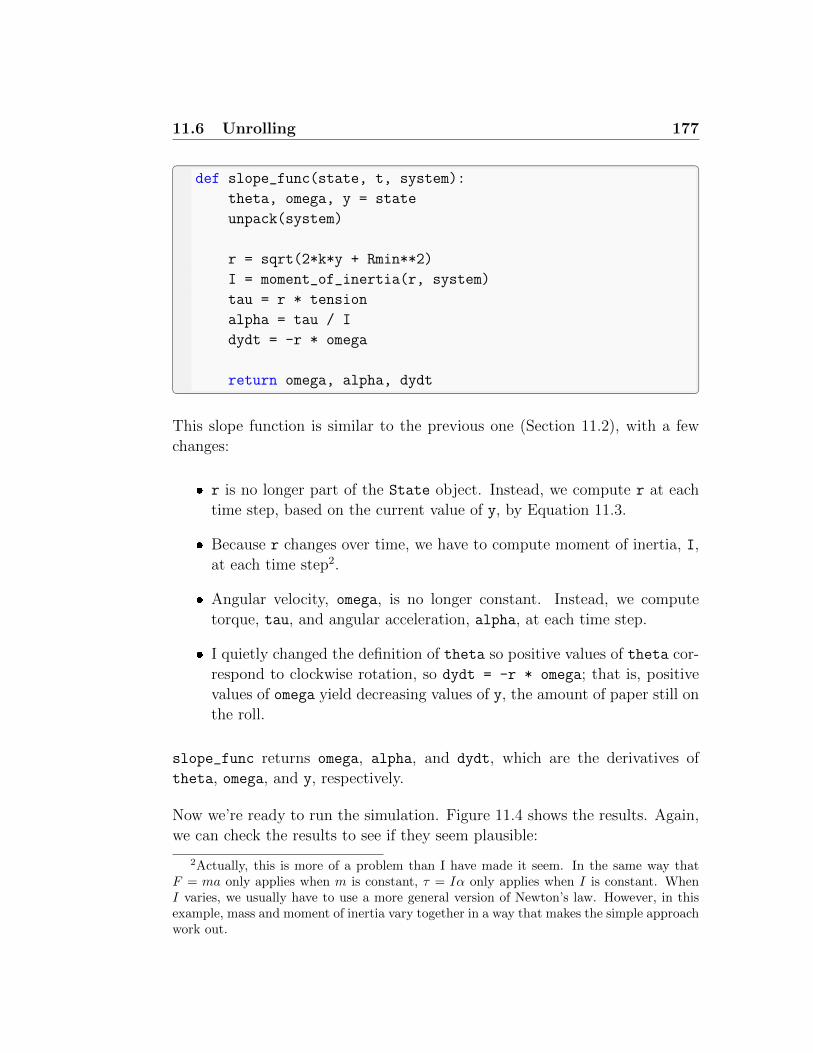
11.6 Unrolling 177
def slope_func(state, t, system):
theta, omega, y = state
unpack(system)
r = sqrt(2*k*y + Rmin**2)
I = moment_of_inertia(r, system)
tau = r * tension
alpha = tau / I
dydt = -r * omega
return omega, alpha, dydt
This slope function is similar to the previous one (Section 11.2), with a few
changes:
� r is no longer part of the State object. Instead, we compute r at each
time step, based on the current value of y, by Equation 11.3.
� Because r changes over time, we have to compute moment of inertia, I,
at each time step2.
� Angular velocity, omega, is no longer constant. Instead, we compute
torque, tau, and angular acceleration, alpha, at each time step.
� I quietly changed the definition of theta so positive values of theta cor-
respond to clockwise rotation, so dydt = -r * omega; that is, positive
values of omega yield decreasing values of y, the amount of paper still on
the roll.
slope_func returns omega, alpha, and dydt, which are the derivatives of
theta, omega, and y, respectively.
Now we’re ready to run the simulation. Figure 11.4 shows the results. Again,
we can check the results to see if they seem plausible:
2Actually, this is more of a problem than I have made it seem. In the same way thatF = ma only applies when m is constant, τ = Iα only applies when I is constant. WhenI varies, we usually have to use a more general version of Newton’s law. However, in thisexample, mass and moment of inertia vary together in a way that makes the simple approachwork out.

178 Chapter 11 Rotation
0 25 50 75 100 125 150 1750
200
400
Ang
le (
rad)
theta
0 25 50 75 100 125 150 1750
2
4
6
Ang
ular
vel
ocity
(ra
d/s)
omega
0 25 50 75 100 125 150 175Time(s)
30
40
Leng
th (
m)
y
Figure 11.4: Simulation results showing rotation, angular velocity, and lengthover time.
� Angular velocity, omega, increases almost linearly at first, as constant
force yields almost constant torque. Then, as the radius decreases, the
lever arm decreases, yielding lower torque, but moment of inertia de-
creases even more, yielding higher angular acceleration.
� The final value of omega is 7.4 rad/s, which is close to one revolution per
second, so that seems plausible.
� The final value of theta is 555 rad, which is about 88 revolutions.
� The final value of y is 21 m of paper left on the roll, which means the
kitten pulled off 26 m in two minutes. That doesn’t seem impossible,
although it is based on a level of consistency and focus that is unlikely
in a kitten.
This model yields results that seem reasonable, but remember that I chose the
force applied by the kitten arbitrarily, and the model ignores friction between
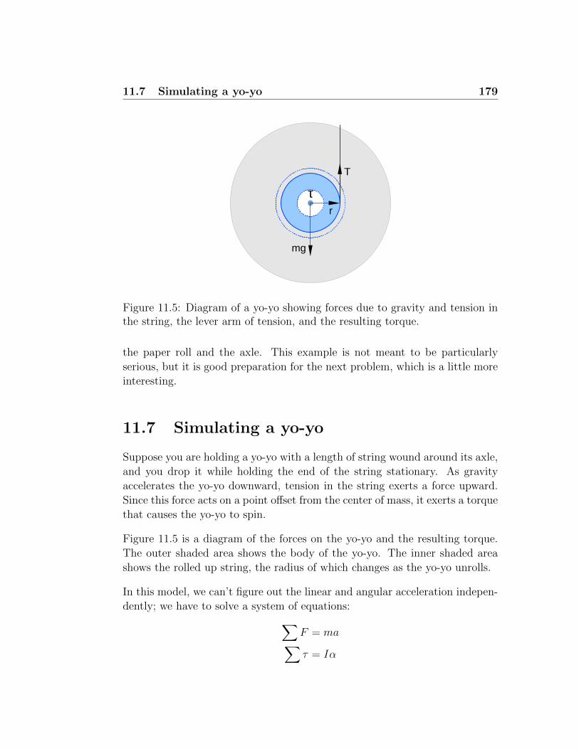
11.7 Simulating a yo-yo 179
r
T
τ
mg
Figure 11.5: Diagram of a yo-yo showing forces due to gravity and tension inthe string, the lever arm of tension, and the resulting torque.
the paper roll and the axle. This example is not meant to be particularly
serious, but it is good preparation for the next problem, which is a little more
interesting.
11.7 Simulating a yo-yo
Suppose you are holding a yo-yo with a length of string wound around its axle,
and you drop it while holding the end of the string stationary. As gravity
accelerates the yo-yo downward, tension in the string exerts a force upward.
Since this force acts on a point offset from the center of mass, it exerts a torque
that causes the yo-yo to spin.
Figure 11.5 is a diagram of the forces on the yo-yo and the resulting torque.
The outer shaded area shows the body of the yo-yo. The inner shaded area
shows the rolled up string, the radius of which changes as the yo-yo unrolls.
In this model, we can’t figure out the linear and angular acceleration indepen-
dently; we have to solve a system of equations:∑F = ma∑τ = Iα

180 Chapter 11 Rotation
where the summations indicate that we are adding up forces and torques.
As in the previous examples, linear and angular velocity are related because
of the way the string unrolls:
dy
dt= −rdθ
dt
In this example, the linear and angular accelerations have opposite sign. As
the yo-yo rotates counter-clockwise, θ increases and y, which is the length of
the rolled part of the string, decreases.
Taking the derivative of both sides yields a similar relationship between linear
and angular acceleration:d2y
dt2= −rd
2θ
dt2
Which we can write more concisely:
a = −rα
This relationship is not a general law of nature; it is specific to scenarios like
this where there is rolling without stretching or slipping.
Because of the way we’ve set up the problem, y actually has two meanings: it
represents the length of the rolled string and the height of the yo-yo, which
decreases as the yo-yo falls. Similarly, a represents acceleration in the length
of the rolled string and the height of the yo-yo.
We can compute the acceleration of the yo-yo by adding up the linear forces:∑F = T −mg = ma
Where T is positive because the tension force points up, and mg is negative
because gravity points down.
Because gravity acts on the center of mass, it creates no torque, so the only
torque is due to tension: ∑τ = Tr = Iα
Positive (upward) tension yields positive (counter-clockwise) angular acceler-
ation.

11.7 Simulating a yo-yo 181
Now we have three equations in three unknowns, T , a, and α, with I, m, g,
and r as known quantities. It is simple enough to solve these equations by
hand, but we can also get SymPy to do it for us:
T, a, alpha, I, m, g, r = symbols('T a alpha I m g r')
eq1 = Eq(a, -r * alpha)
eq2 = Eq(T - m*g, m * a)
eq3 = Eq(T * r, I * alpha)
soln = solve([eq1, eq2, eq3], [T, a, alpha])
The results are
T = mgI/I∗
a = −mgr2/I∗
α = mgr/I∗
where I∗ is the augmented moment of inertia, I +mr2.
To simulate the system, we don’t really need T ; we can plug a and α directly
into the slope function.
At this point you have everything you need to simulate the descent of a yo-
yo. In the notebook for this chapter you will have a chance to finish off the
exercise.

182 Chapter 11 Rotation

Chapter 12
Second order systems

184 Chapter 12 Second order systems

Index
error_func, 125
fit_leastsq, 124, 126
interp_inverse, 136, 156
make_system, 69, 103, 125, 139,
141, 149, 162, 170
max_bounded, 157
minimize_scalar, 157
read_html, 32
run_analysis, 111
run_odeint, 123, 126, 135, 140, 152
run_simulation, 71, 85, 102, 120
to, 148
abstraction, xi
acceleration, 132, 151
air resistance, 2, 133, 137, 146
algebra, 59
Anaconda, xvii
analysis, xi, 3, 59, 94, 110, 165
angle, 147, 151
angular acceleration, 167
angular velocity, 161, 172
animation, 153
argument, 6, 8, 32
array, 28, 34, 37, 94, 147
assert statement, 107
assignment, 74
assignment operator, 23
bag of blood, 127
basal level, 128
baseball, 145
basic reproduction number, 92
bike share system, 4
bikeshare, 17
birth rate, 53
body, 7
boolean, 11
bottom up, xiv
Box, George, 2, 17
bracket operator, 33, 35, 74
calculus, xv
call, 8
carrying capacity, 46, 53
code block, 7
code quality, 21
coffee cooling problem, 97
color, 34
columns, 33
comment, 20
comparison operator, 23
compartment model, 68, 115
component, 147
concatenation, 87
concentration, 117
Condition object, 138, 141, 149,
157, 162, 169

186 INDEX
conduction, 99
conservation of energy, 106
constant growth, 34
constant of integration, 58, 93
contact number, 92
continuous, 57
contributors, xviii
convection, 99
cross product, 167
cubic spline, 136
cylinder, 169
data, xii, 32, 43, 98, 117
DataFrame, 32, 33
DataFrame object, 74, 90, 117
debugging, 16, 30
decorate, 39, 73
def, 7
defining functions, 7
deg2rad, 148, 150
degree, 148
demography, 55
density, 99, 106, 137, 149, 170
derivative, 120
design, xii, 66
deterministic, 24
diabetes, 114
differential equation, 57, 62, 68,
129, 132, 161
dimensionless, 91
dimensions, 148
discrete, 57
disease, 66
docstring, 20
documentation, 20
dot operator, 5, 33, 75, 150
drag coefficient, 137, 146
drag equation, 137, 151
drag force, 137, 151
dropna, 54
ellipse, xii
else clause, 12
Empire State Building, 1
epidemic, 65
equality, 23
equilibrium, 45
Erlich, Paul, 31
error
syntax, 24
error function, 104, 124, 142
error message, 16
Euler’s method, 122
explanation, xii, 29
exponential growth, 63
exponentiation, 58
falling penny, 133
False, 11
Fenway Park, 145
first order ODE, 131
fitting data, 43, 122, 124
flip, 11
flow, 68
fluid flow, 100
for loop, 15
force
drag, 137
forward problem, 143
free parameter, 117
Freshman Plague, 65, 76
FSIGT, 114
fsolve, 104, 142, 158
Function
slope, 163
function, 4, 7
as parameter, 42

INDEX 187
as return value, 117
error, 104, 142
slope, 123, 133, 140, 150, 170
update, 41, 70, 119
function error, 124
general solution, 63
geometric progression, 56
Git, xvii
GitHub, xvii
glucose, 113
glucose effectiveness, 127
gravity, 2, 140
Green Monster, 145
gyroscopic precession, 159
hard coding, 36
hash symbol, 20
heat, 98
heat transfer, 99
herd immunity, 78, 83
hyperglycemia, 114
idxmax, 76, 155
if statement, 12, 24
immunization, 76
implementation, 68
import statement, 4, 32, 61
incremental development, 30
indentation, 7, 12
index, 33
infection, 66
infection rate, 67
insulin, 113
insulin minimal model, 129
insulin sensitivity, 127
Int64Index, 34
intalling Python, xvi
integration, 58, 93, 165
internal validation, xiii
interp1d, 117
interpolate, 117, 136, 156
interpolation, 117
interstitial fluid, 115
inverse problem, 143
iterative modeling, xii, 17, 35
Jupyter, xv, xviii
Kermack-McKendrick, 65
Kermack-McKendrick model, 85
kitten, 166, 172
label, 34
launch angle, 146
leastsq, 124
legend, 34
lever arm, 167, 173
linear multistep method, 122
linrange, 37, 118, 133
linspace, 28, 37, 88, 94
lmdif, 124
loc, 74, 155
local variables, 22
logarithm, 58
logistic curve, 80
logistic function, 64
logistic growth, 64
loop, 15, 28, 37
loop variable, 15, 28, 37
LSODA, 123
magic command, 6
magnitude, 147, 151, 167
Magnus force, 146
mass, 168
math notation, 60
Mathematica, 61

188 INDEX
mathematical model, 1
Matplotlib, xiv, 7
max, 76
mean squared error, 124
measles, 78
metric, 24, 27, 75
minimal model, 114
MINPACK, 124
missing data, 54
mixing, 106
model, xi
modeling, xi
modsim library, xv
moment of inertia, 168
monotonic, 136, 152
mortality rate, 53
Mount Everest, 99
MSE, 124
myth, 1
Mythbusters, 2, 138
NaN, 54
NASA, 146
newfig, 6
Newton, xii, 1
Newton’s law of cooling, 100
Newton’s second law of motion, 132
non-spatial model, 127
nondimensionalization, 91
not a number, 54
NumPy, xiv, 28, 147
Occam’s Razor, 115
odeint, 123
ODEPACK, 123
Olin College, 4, 65
operator, 22
assignment, 23
bracket, 33, 35
comparison, 23
dot, 5, 33, 75, 150
mathematical, 3
scatter, 125
update, 6
operator bracket, 74
optimization, 82, 108, 156
OptimizeResult object, 157
optional parameter, 14
orbit, xii
ordinary differential equation, 123
Orwell, George, 17
override, 14
pancreas, 113
Pandas, xiv, 32, 36, 54
parabola, 135
parameter, 9, 18, 43
of a function, 27
of a model, 27
optional, 14
parameter of a system, 143
parameter sweep, 29, 78, 87, 156
parameterize, 46
parentheses, 8
particular solution, 63
patient zero, 95
penny, 1
pharmacokinetics, 113
Pint, xiv, 133, 152, 161
Plato, 60
plot, 6, 34, 39, 73, 153
pol2cart, 148
population, 31
Population Bomb, 31
position, 132
prediction, xii, 29, 31, 51
print statement, 10

INDEX 189
probability, 13, 18
programming languages, 60
projection, 51
proof, 59
proportional growth, 39
quadratic growth, 43, 51, 56, 64
quality of fit, 43, 122
quantum mechanics, 132
quarter, 141
radian, 147, 161
radiation, 99, 101
Ramirez, Manny, 145
range, 15, 154
realism, xii, 18
recovery rate, 67
recurrence relation, 56
reference area, 137
regime, 44, 59
relativity, xii, 132
repository, xvii
return statement, 22, 26
return value, 26, 70
rolling, 174
root, 104
rotation, 159
scaffolding, 30
scalar, 151, 157, 159, 168
scatter operator, 125
SciPy, xiv, 117, 124, 157
second order ODE, 131
sequence, 33
Series, 32, 76, 91, 117, 126
series, 33, 94
simplicity, xii
simulation, 3, 36
single valued, 136
SIR model, 65, 85
sleep, 154
slice index, 155
slope function, 123, 133, 140, 150,
163, 170
specific heat, 106
specific heat capacity, 99
spline, 136
sqrt, 4
state, 5
State object, 68, 70, 101, 119, 133,
134, 150, 163
state variable, 68, 150
statement
assert, 107
if, 12, 24
import, 32, 61
print, 10
return, 22, 26
stochastic, 24
stock, 68
stock and flow diagram, 68
str function, 88
string, 11, 33, 87
style, 7
style string, 7
susceptible, 67
sweep, 29, 77
SweepFrame object, 90
SweepSeries object, 78, 87, 156
Symbol, 61
Symbol object, 62
symbolic computation, 60
symbolic manipulation, 59
SymPy, xiv, 61, 62, 110, 174
syntax error, 24
system, xi
System object, 4, 19, 38, 52, 68, 86,

190 INDEX
101, 119, 123, 125, 133, 139,
149, 162
system of equations, 134, 173
system variable, 5, 75
temperature, 98
temporary variable, 22
tensor, 168
terminal velocity, 138, 140
testable change, 30
thermal mass, 99
thermal system, 97
time dependent, 120, 134
time series, 36
time step, 12, 57, 59, 70–72, 101–
103, 120, 122, 171
TimeFrame object, 72, 74, 103, 124,
135, 152
TimeSeries object, 36, 39, 72
toilet paper, 160
top down, xiv
torque, 167, 173
trajectory plot, 153
True, 11
unit, 4, 133, 147
United Nations, 34
United States Census Bureau, 34
unpack, 86, 102, 111, 120, 123, 134,
139–141, 150, 162, 169
update function, 41, 70, 119
update operator, 6
vaccine, 76
validation, xii
internal, xiii
value, 3
values, 33
variable, 3
loop, 28
temporary, 22
variable mass, 132
variables
local, 22
vector, 167
Vector object, 147
vector operation, 147
velocity, 132, 137, 145, 151
volume, 106
Walker, Jearl, 97
Wellesley College, 4
what if scenario, 29
Wikipedia, 31
WolframAlpha, 60
world population, 31
yo-yo, 173
Zen of Python, 139
zip, 154