Embed Size (px)
DESCRIPTION
Atoll calibration way
Citation preview
Measurement Module Atoll 3.1.2
© Forsk 2012 Confidential – Do not share without prior permission Slide 1

1. SPM Calibration Concepts
2. Guidelines for CW Measurement Surveys
3. Working With CW Measurements
4. Automatic Calibration Method
5. Analysing the Calibrated Model
6. Calibration Process Summary
Training Programme
© Forsk 2012 Confidential – Do not share without prior permission Slide 2
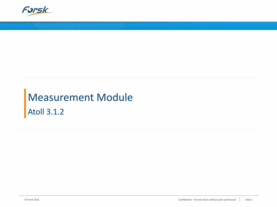
1. SPM Calibration Concepts
Purpose of Model Calibration
Introduction to the Standard Propagation Model (SPM)
Requirements
Quality targets
© Forsk 2012 Confidential – Do not share without prior permission Slide 3
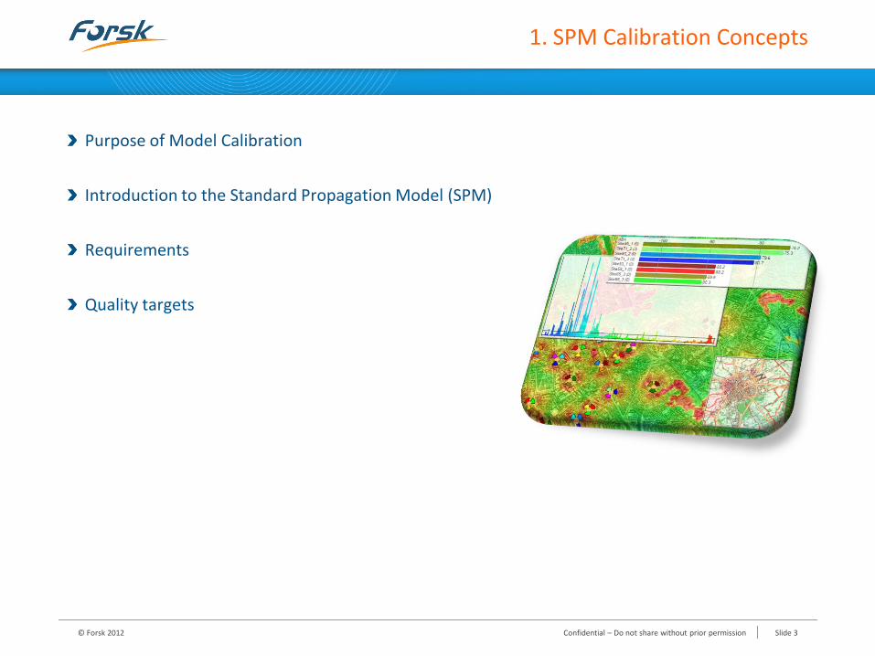
Purpose of Model Calibration
The propagation model is the basis of cell planning in mobile networks
Reliability of cell planning is closely related to the propagation model accuracy
A good model calibration is therefore required
To obtain a propagation model consistent with the actual radio environment
To improve the accuracy of coverage predictions
To properly estimate interference
The model calibration process entails three main procedures:
Collecting CW (Continuous Wave) measurement data
• Site location
• Constructing test platform
• Drive test
Post-processing the CW measurement data
• Data filtering
Calibrating the model
© Forsk 2012 Slide 4 Confidential – Do not share without prior permission
Introduction to the Standard Propagation Model (SPM)
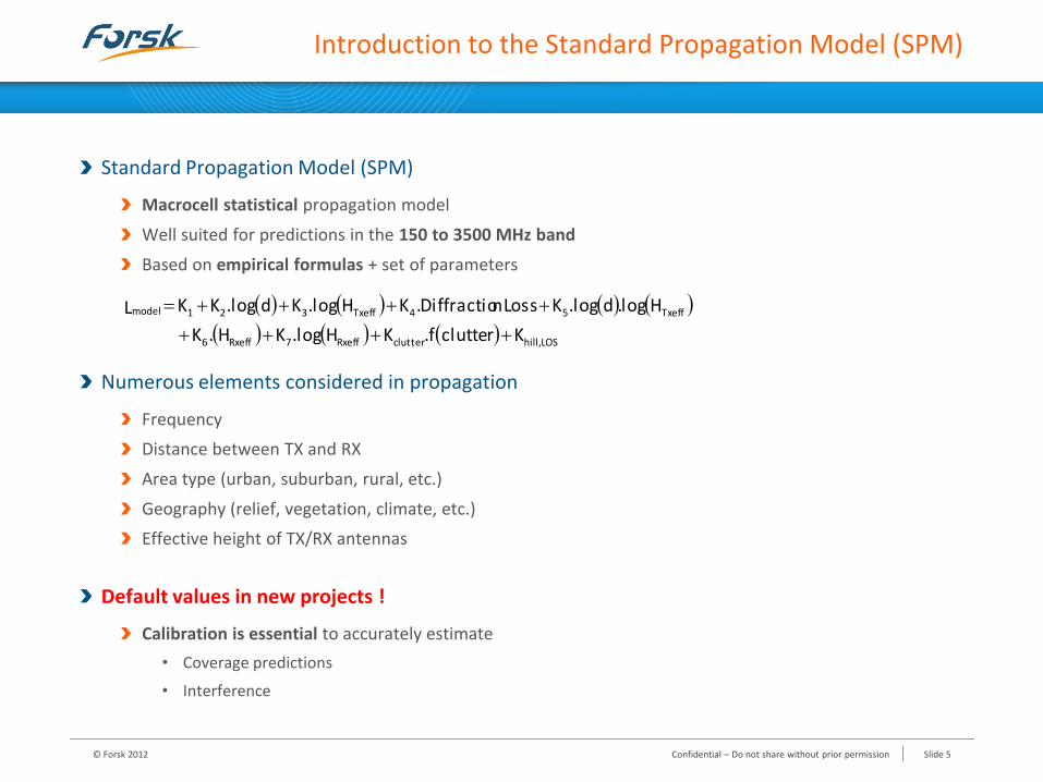
Standard Propagation Model (SPM)
Macrocell statistical propagation model
Well suited for predictions in the 150 to 3500 MHz band
Based on empirical formulas + set of parameters
Numerous elements considered in propagation
Frequency
Distance between TX and RX
Area type (urban, suburban, rural, etc.)
Geography (relief, vegetation, climate, etc.)
Effective height of TX/RX antennas
Default values in new projects !
Calibration is essential to accurately estimate
• Coverage predictions
• Interference
© Forsk 2012 Confidential – Do not share without prior permission Slide 5
LOS hill,clutterRxeff7Rxeff6
Txeff54Txeff321model
Kclutter.fKH.logKH.K
Hlog.d.logKLoss nDiffractio.KH.logKd.logKKL
Requirements (1/2)
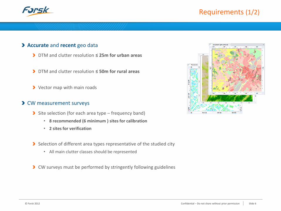
Accurate and recent geo data
DTM and clutter resolution ≤ 25m for urban areas
DTM and clutter resolution ≤ 50m for rural areas
Vector map with main roads
CW measurement surveys
Site selection (for each area type – frequency band)
• 8 recommended (6 minimum ) sites for calibration
• 2 sites for verification
Selection of different area types representative of the studied city
• All main clutter classes should be represented
CW surveys must be performed by stringently following guidelines
© Forsk 2012 Confidential – Do not share without prior permission Slide 6
Requirements (2/2)
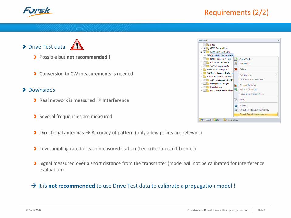
Drive Test data
Possible but not recommended !
Conversion to CW measurements is needed
Downsides
Real network is measured Interference
Several frequencies are measured
Directional antennas Accuracy of pattern (only a few points are relevant)
Low sampling rate for each measured station (Lee criterion can’t be met)
Signal measured over a short distance from the transmitter (model will not be calibrated for interference evaluation)
It is not recommended to use Drive Test data to calibrate a propagation model !
© Forsk 2012 Confidential – Do not share without prior permission Slide 7
Quality Targets
Overall objective :
Minimize the error between the propagation model and the CW survey data
Quality targets for calibration sites
Global mean error on calibration sites < 1 dB
Global standard deviation on calibration sites < 8 dB
Mean error on each calibration site < 2.5 dB
Standard deviation on each calibration site < 8.5 dB
Quality targets for verification sites
Global mean error on verification sites < 2 dB
Global standard deviation on verification sites < 8.5 dB
© Forsk 2012 Confidential – Do not share without prior permission Slide 8
1. SPM Calibration Concepts
2. Guidelines for CW Measurement Surveys
3. Working With CW Measurements
4. Automatic Calibration Method
5. Analysing the Calibrated Model
6. Calibration Process Summary
Training Programme
© Forsk 2012 Confidential – Do not share without prior permission Slide 9
2. Guidelines for CW Measurement Surveys
Site Preselection criteria
Survey route criteria
Radio criteria
© Forsk 2012 Confidential – Do not share without prior permission Slide 10
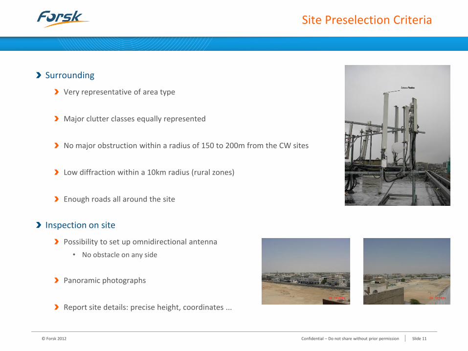
Site Preselection Criteria
Surrounding
Very representative of area type
Major clutter classes equally represented
No major obstruction within a radius of 150 to 200m from the CW sites
Low diffraction within a 10km radius (rural zones)
Enough roads all around the site
Inspection on site
Possibility to set up omnidirectional antenna
• No obstacle on any side
Panoramic photographs
Report site details: precise height, coordinates ...
© Forsk 2012 Confidential – Do not share without prior permission Slide 11
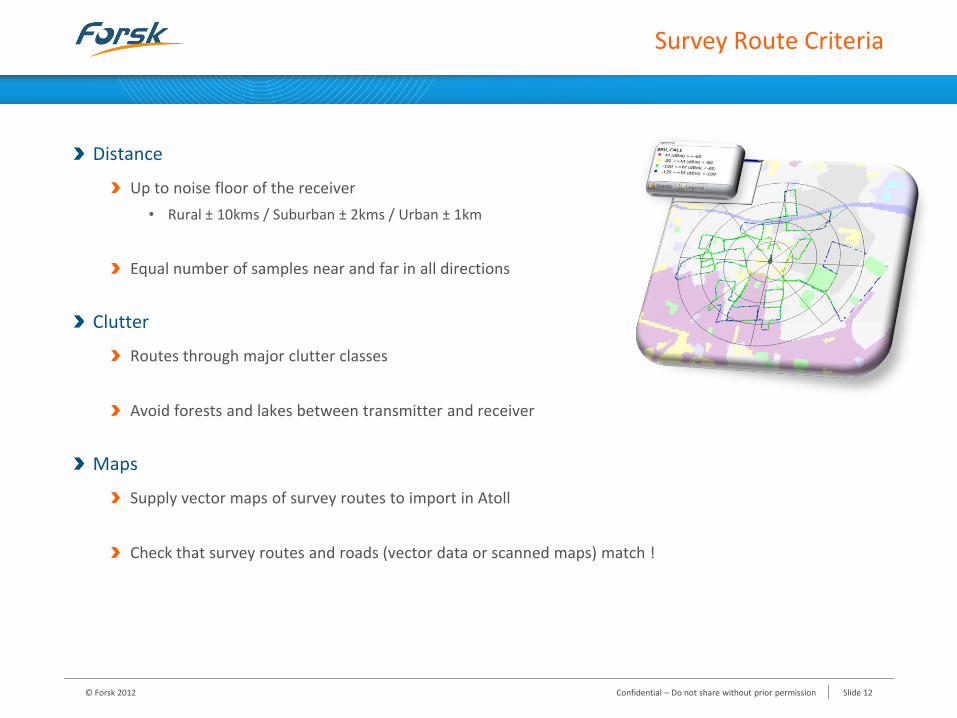
Survey Route Criteria
Distance
Up to noise floor of the receiver
• Rural ± 10kms / Suburban ± 2kms / Urban ± 1km
Equal number of samples near and far in all directions
Clutter
Routes through major clutter classes
Avoid forests and lakes between transmitter and receiver
Maps
Supply vector maps of survey routes to import in Atoll
Check that survey routes and roads (vector data or scanned maps) match !
© Forsk 2012 Confidential – Do not share without prior permission Slide 12
Radio Criteria (1)
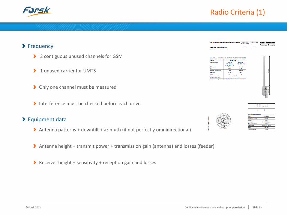
Frequency
3 contiguous unused channels for GSM
1 unused carrier for UMTS
Only one channel must be measured
Interference must be checked before each drive
Equipment data
Antenna patterns + downtilt + azimuth (if not perfectly omnidirectional)
Antenna height + transmit power + transmission gain (antenna) and losses (feeder)
Receiver height + sensitivity + reception gain and losses
© Forsk 2012 Confidential – Do not share without prior permission Slide 13
Radio Criteria (2)
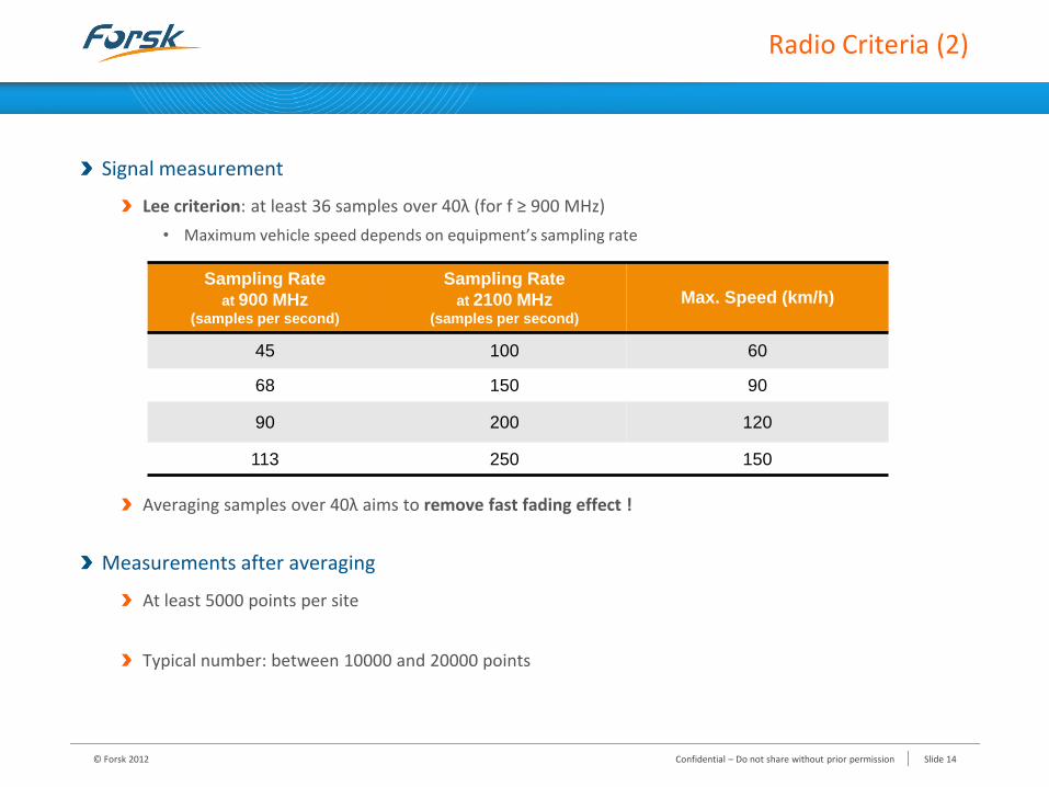
Signal measurement
Lee criterion: at least 36 samples over 40λ (for f ≥ 900 MHz)
• Maximum vehicle speed depends on equipment’s sampling rate
Averaging samples over 40λ aims to remove fast fading effect !
Measurements after averaging
At least 5000 points per site
Typical number: between 10000 and 20000 points
Sampling Rate
at 900 MHz (samples per second)
Sampling Rate
at 2100 MHz (samples per second)
Max. Speed (km/h)
45 100 60
68 150 90
90 200 120
113 250 150
© Forsk 2012 Confidential – Do not share without prior permission Slide 14

1. SPM Calibration Concepts
2. Guidelines for CW Measurement Surveys
3. Working With CW Measurements
4. Automatic Calibration Method
5. Analysing the Calibrated Model
6. Calibration Process Summary
Training Programme
© Forsk 2012 Confidential – Do not share without prior permission Slide 15
3. Working with CW Measurements
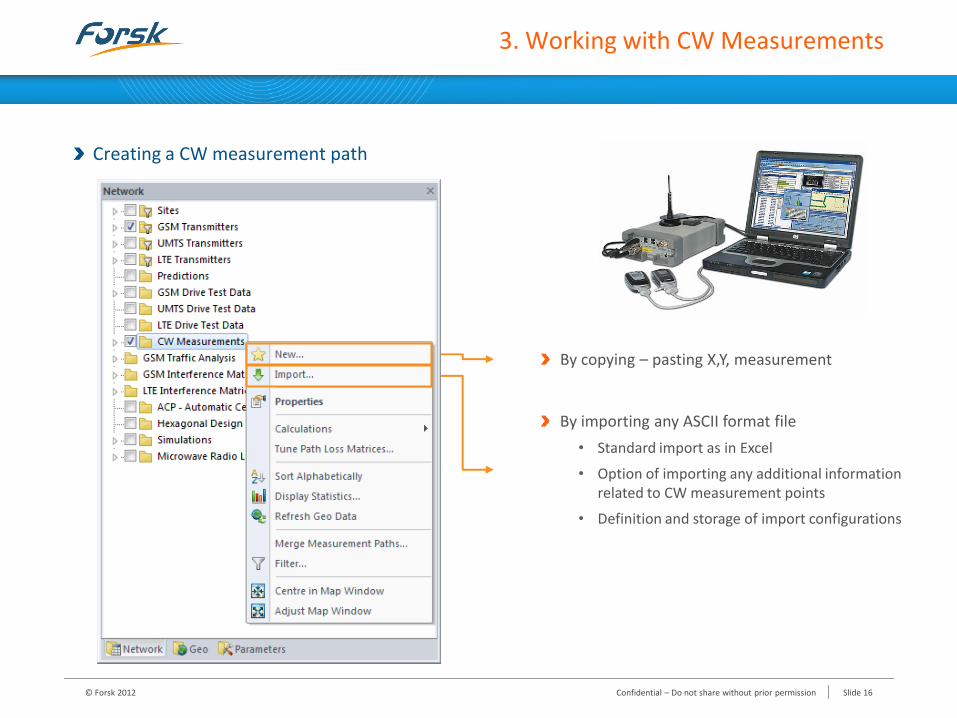
Creating a CW measurement path
By importing any ASCII format file
• Standard import as in Excel
• Option of importing any additional information related to CW measurement points
• Definition and storage of import configurations
By copying – pasting X,Y, measurement
© Forsk 2012 Confidential – Do not share without prior permission Slide 16
3. Working With CW Measurements
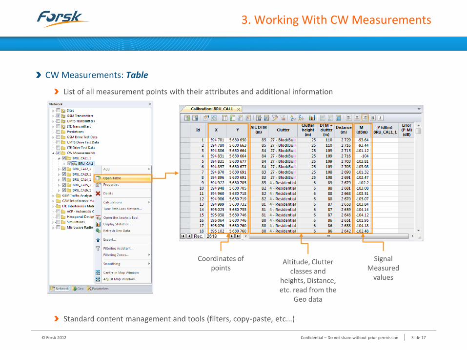
CW Measurements: Table
List of all measurement points with their attributes and additional information
Standard content management and tools (filters, copy-paste, etc...)
Coordinates of points
Signal Measured
values
Altitude, Clutter classes and
heights, Distance, etc. read from the
Geo data
© Forsk 2012 Confidential – Do not share without prior permission Slide 17
3. Working With CW Measurements
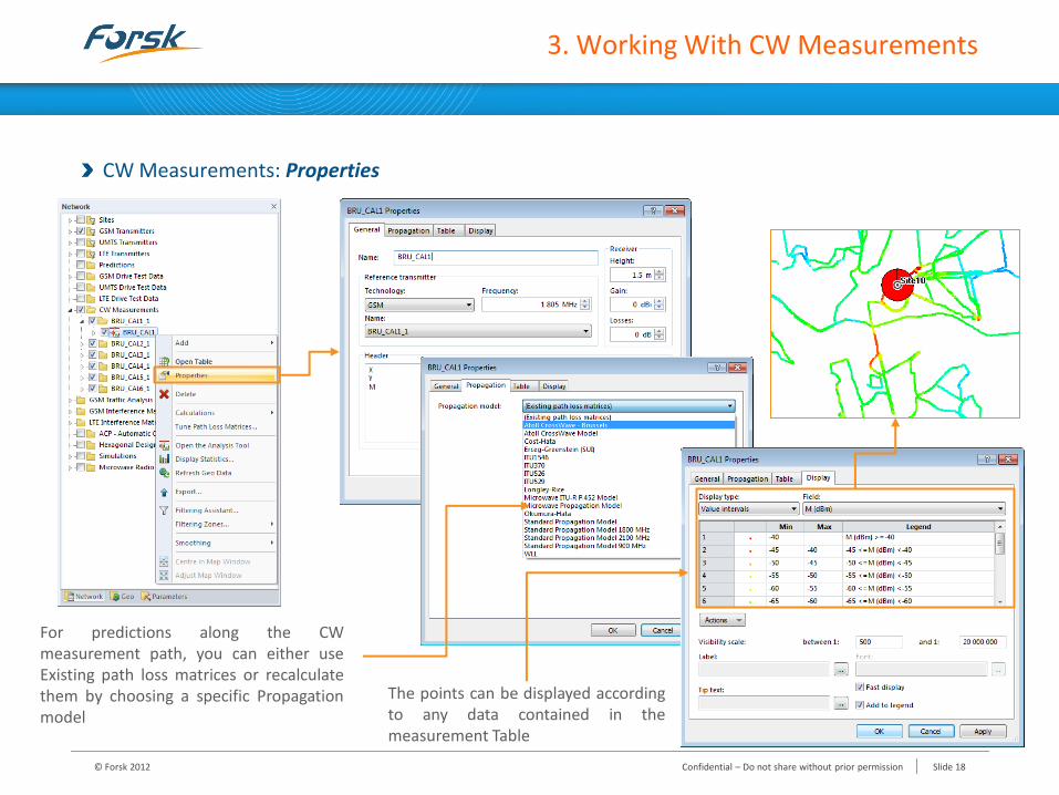
CW Measurements: Properties
The points can be displayed according to any data contained in the measurement Table
For predictions along the CW measurement path, you can either use Existing path loss matrices or recalculate them by choosing a specific Propagation model
© Forsk 2012 Confidential – Do not share without prior permission Slide 18
3. Working With CW Measurements
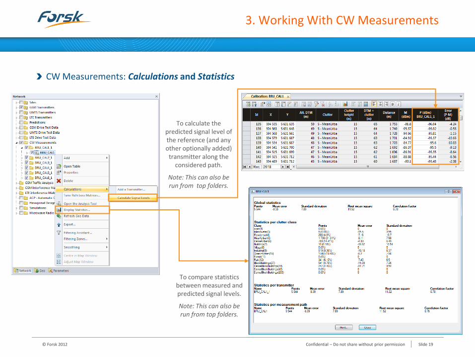
CW Measurements: Calculations and Statistics
To calculate the predicted signal level of the reference (and any other optionally added)
transmitter along the considered path.
Note: This can also be run from top folders.
To compare statistics between measured and predicted signal levels.
Note: This can also be run from top folders.
© Forsk 2012 Confidential – Do not share without prior permission Slide 19
3. Working With CW Measurements
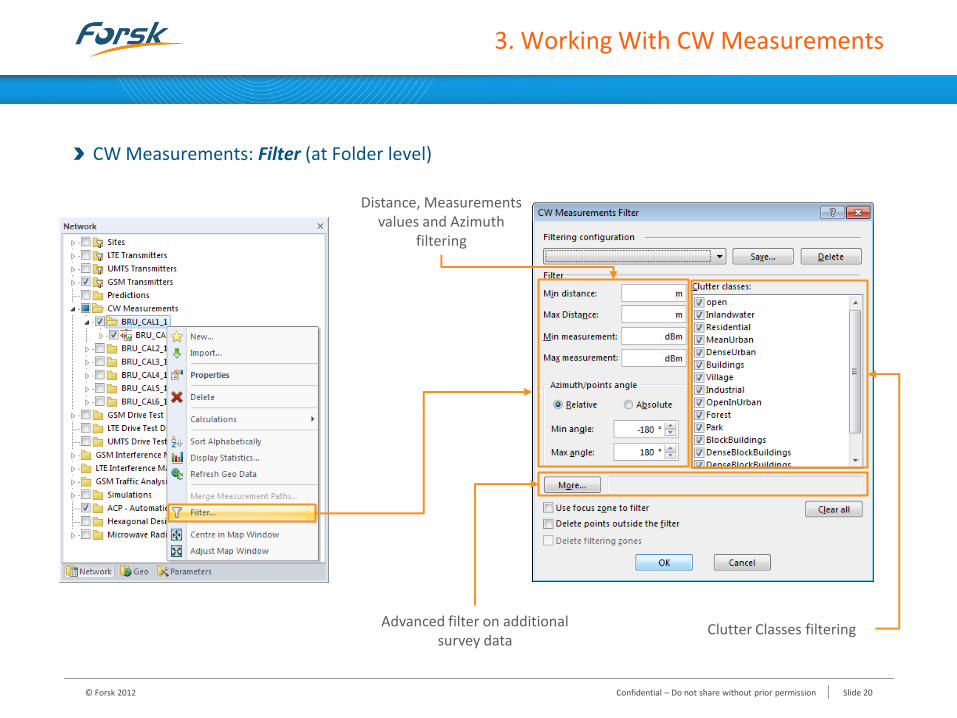
CW Measurements: Filter (at Folder level)
Distance, Measurements
values and Azimuth filtering
Advanced filter on additional survey data
Clutter Classes filtering
© Forsk 2012 Confidential – Do not share without prior permission Slide 20
3. Working With CW Measurements
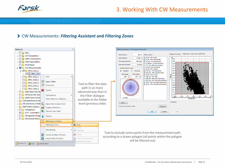
CW Measurements: Filtering Assistant and Filtering Zones
Tool to filter the data path in an more
advanced way than in the Filter dialogue
available at the folder level (previous slide)
Tool to exclude some points from the measurement path according to a drawn polygon (all points within the polygon
will be filtered out)
© Forsk 2012 Confidential – Do not share without prior permission Slide 21
3. Working With CW Measurements
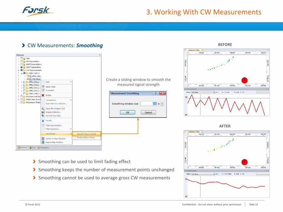
CW Measurements: Smoothing
Smoothing can be used to limit fading effect
Smoothing keeps the number of measurement points unchanged
Smoothing cannot be used to average gross CW measurements
BEFORE
AFTER
Create a sliding window to smooth the measured signal strength
© Forsk 2012 Confidential – Do not share without prior permission Slide 22
3. Working With CW Measurements
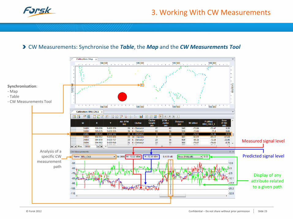
CW Measurements: Synchronise the Table, the Map and the CW Measurements Tool
Synchronisation: - Map - Table - CW Measurements Tool
Analysis of a specific CW
measurement path
Measured signal level
Predicted signal level
Display of any attribute related to a given path
© Forsk 2012 Confidential – Do not share without prior permission Slide 23

1. SPM Calibration Concepts
2. Guidelines for CW Measurement Surveys
3. Working With CW Measurements
4. Automatic Calibration Method
5. Analysing the Calibrated Model
6. Calibration Process Summary
Training Programme
© Forsk 2012 Confidential – Do not share without prior permission Slide 24
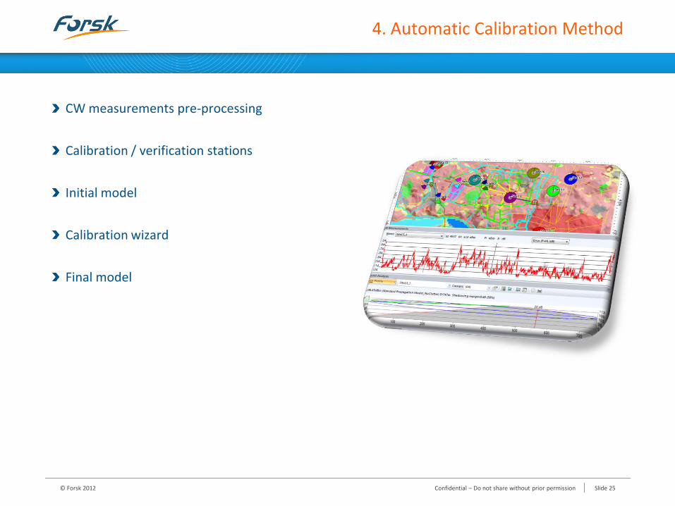
4. Automatic Calibration Method
CW measurements pre-processing
Calibration / verification stations
Initial model
Calibration wizard
Final model
© Forsk 2012 Confidential – Do not share without prior permission Slide 25
CW Measurements Pre-processing
Correspondence between Measurements and Geo data
Projection checking
• Check that CW measurements and roads (from vector maps) match
Routes checking
• Check that CW measurements respect planned survey routes
Surrounding checking
• Check, with panoramic photographs, that there is no obstacle
• Option of setting an angle filter to avoid attenuation due to obstacles
© Forsk 2012 Confidential – Do not share without prior permission Slide 26
CW Measurements Pre-processing
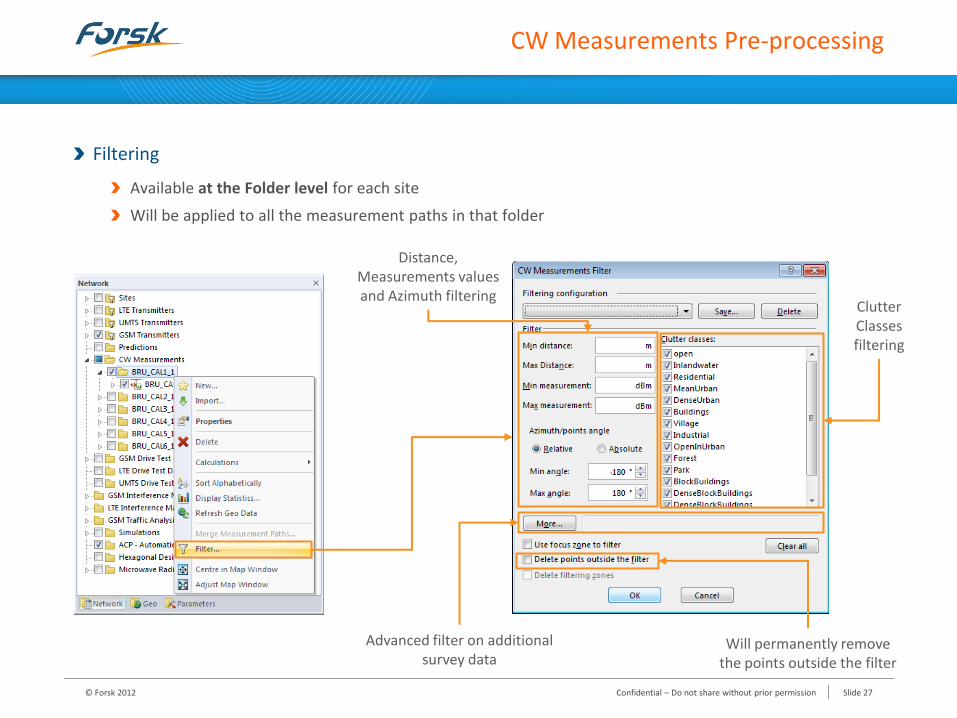
Filtering
Available at the Folder level for each site
Will be applied to all the measurement paths in that folder
Distance,
Measurements values and Azimuth filtering
Advanced filter on additional survey data
Clutter Classes filtering
Will permanently remove the points outside the filter
© Forsk 2012 Confidential – Do not share without prior permission Slide 27
CW Measurements Pre-processing
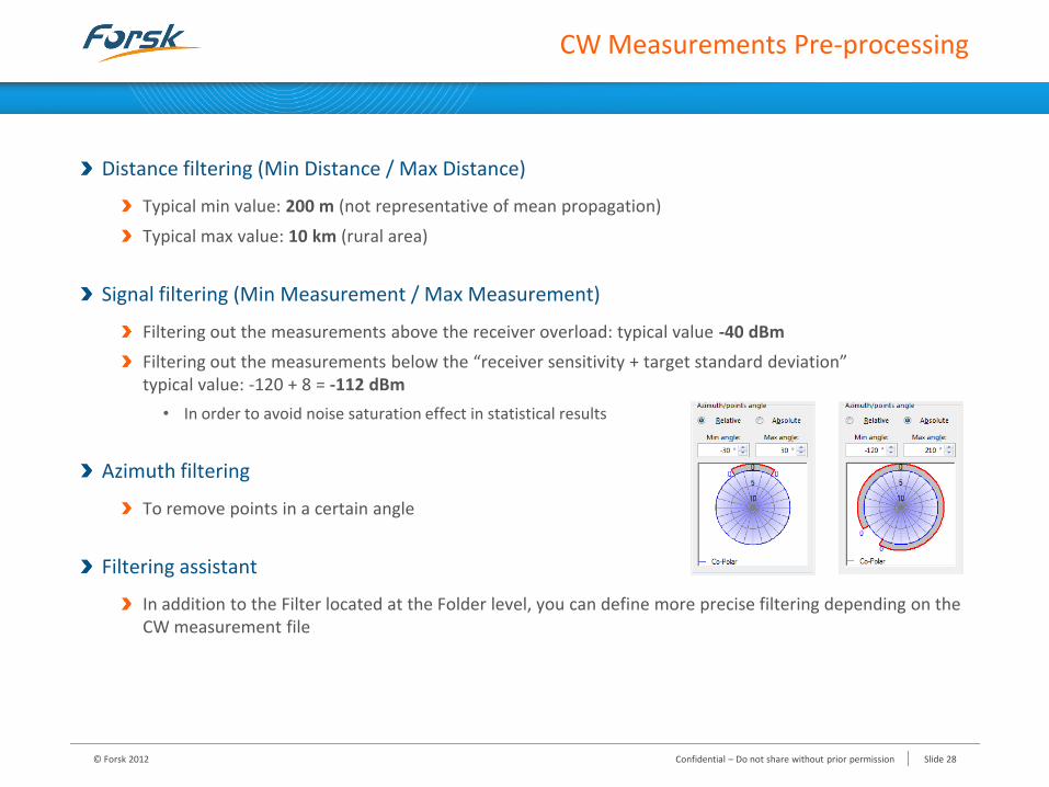
Distance filtering (Min Distance / Max Distance)
Typical min value: 200 m (not representative of mean propagation)
Typical max value: 10 km (rural area)
Signal filtering (Min Measurement / Max Measurement)
Filtering out the measurements above the receiver overload: typical value -40 dBm
Filtering out the measurements below the “receiver sensitivity + target standard deviation” typical value: -120 + 8 = -112 dBm
• In order to avoid noise saturation effect in statistical results
Azimuth filtering
To remove points in a certain angle
Filtering assistant
In addition to the Filter located at the Folder level, you can define more precise filtering depending on the CW measurement file
© Forsk 2012 Confidential – Do not share without prior permission Slide 28
CW Measurements Pre-processing
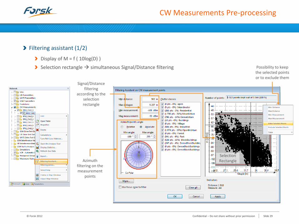
Filtering assistant (1/2)
Display of M = f ( 10log(D) )
Selection rectangle simultaneous Signal/Distance filtering
Signal/Distance filtering
according to the selection rectangle
Selection Rectangle Azimuth
filtering on the measurement
points
Possibility to keep the selected points or to exclude them
© Forsk 2012 Confidential – Do not share without prior permission Slide 29
CW Measurements Pre-processing
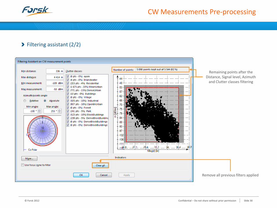
Filtering assistant (2/2)
Remaining points after the Distance, Signal level, Azimuth
and Clutter classes filtering
Remove all previous filters applied
© Forsk 2012 Confidential – Do not share without prior permission Slide 30
CW Measurements Pre-processing
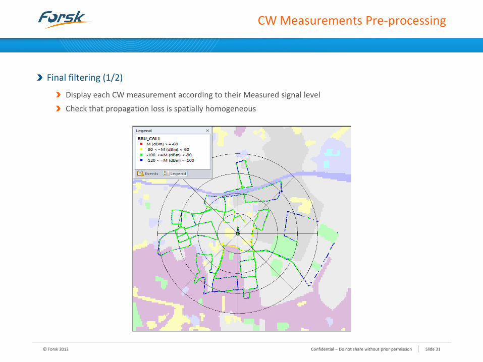
Final filtering (1/2)
Display each CW measurement according to their Measured signal level
Check that propagation loss is spatially homogeneous
© Forsk 2012 Confidential – Do not share without prior permission Slide 31
CW Measurements Pre-processing
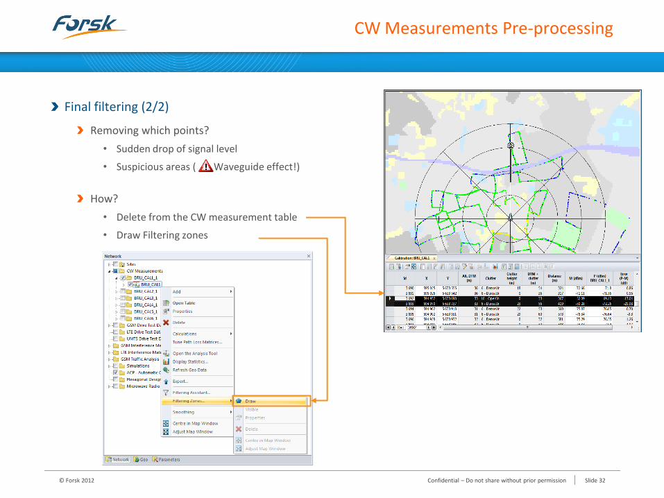
Final filtering (2/2)
Removing which points?
• Sudden drop of signal level
• Suspicious areas ( Waveguide effect!)
How?
• Delete from the CW measurement table
• Draw Filtering zones
© Forsk 2012 Confidential – Do not share without prior permission Slide 32
Calibration / Verification Stations
Calibration stations
Stations so that measurements cover the whole area
Avoid keeping stations with a lot of common points
Verification stations
Stations so that measurements are inside covered area (not at edges!)
Major part of their covered areas are also covered by calibration stations
How many ?
If 7-8 measured stations:
• 6 for calibration; 1-2 for verification
If < 7 measured stations:
• All stations used for calibration
• Verification performed with same stations
© Forsk 2012 Confidential – Do not share without prior permission Slide 33
Initial Model
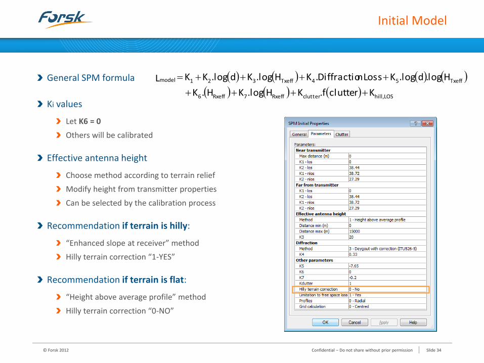
General SPM formula
Ki values
Let K6 = 0
Others will be calibrated
Effective antenna height
Choose method according to terrain relief
Modify height from transmitter properties
Can be selected by the calibration process
Recommendation if terrain is hilly:
“Enhanced slope at receiver” method
Hilly terrain correction “1-YES”
Recommendation if terrain is flat:
“Height above average profile” method
Hilly terrain correction “0-NO”
LOS hill,clutterRxeff7Rxeff6
Txeff54Txeff321model
Kclutter.fKH.logKH.K
Hlog.d.logKLoss nDiffractio.KH.logKd.logKKL
© Forsk 2012 Confidential – Do not share without prior permission Slide 34
Initial Model
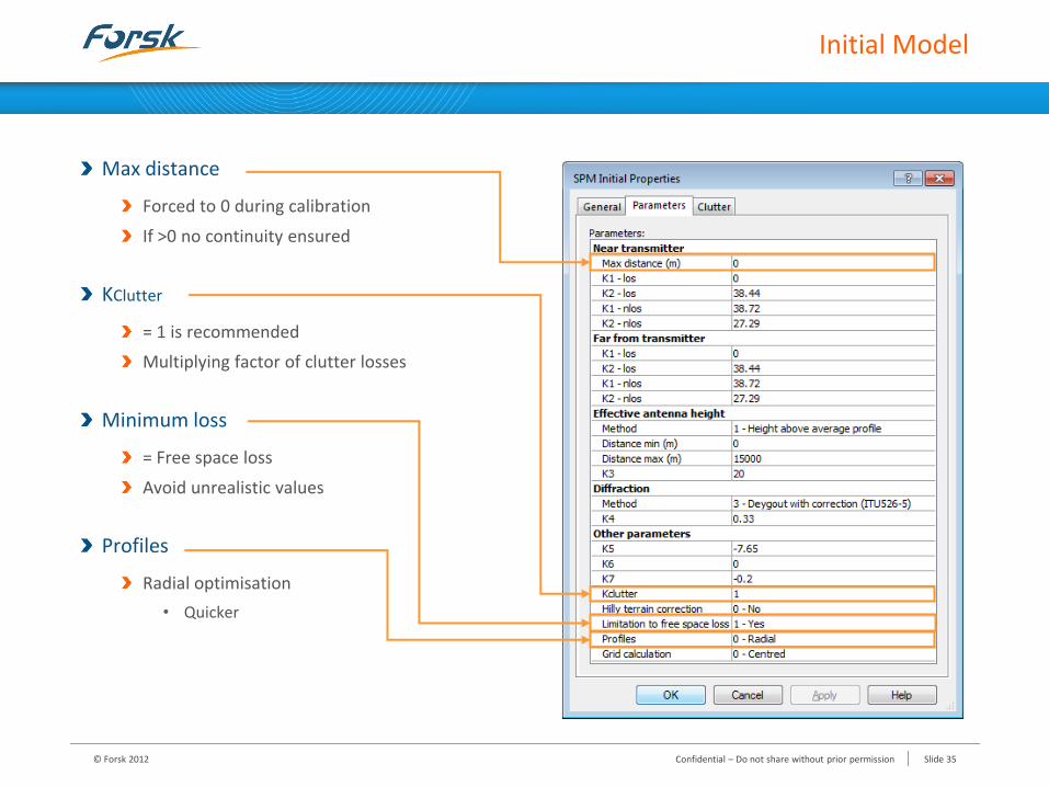
Max distance
Forced to 0 during calibration
If >0 no continuity ensured
KClutter
= 1 is recommended
Multiplying factor of clutter losses
Minimum loss
= Free space loss
Avoid unrealistic values
Profiles
Radial optimisation
• Quicker
© Forsk 2012 Confidential – Do not share without prior permission Slide 35
Initial Model
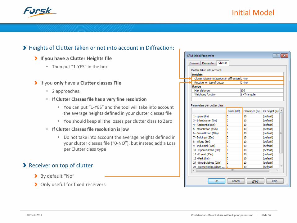
Heights of Clutter taken or not into account in Diffraction:
If you have a Clutter Heights file
• Then put “1-YES” in the box
If you only have a Clutter classes File
• 2 approaches:
• If Clutter Classes file has a very fine resolution
• You can put “1-YES” and the tool will take into account the average heights defined in your clutter classes file
• You should keep all the losses per clutter class to Zero
• If Clutter Classes file resolution is low
• Do not take into account the average heights defined in your clutter classes file (“0-NO”), but instead add a Loss per Clutter class type
Receiver on top of clutter
By default “No”
Only useful for fixed receivers
© Forsk 2012 Confidential – Do not share without prior permission Slide 36
Initial Model
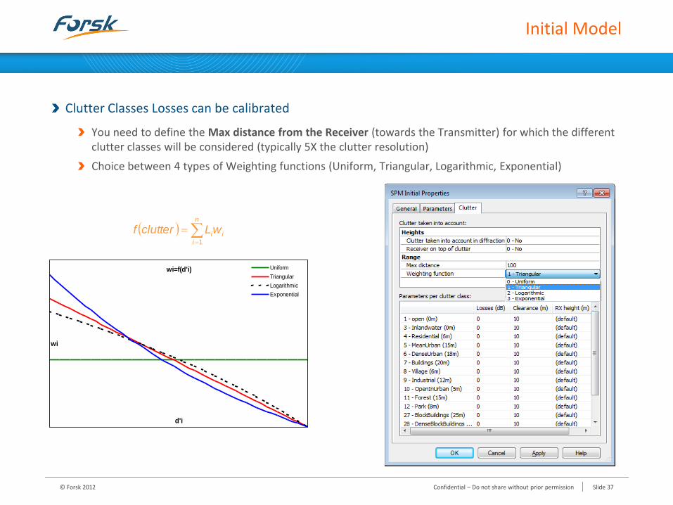
Clutter Classes Losses can be calibrated
You need to define the Max distance from the Receiver (towards the Transmitter) for which the different clutter classes will be considered (typically 5X the clutter resolution)
Choice between 4 types of Weighting functions (Uniform, Triangular, Logarithmic, Exponential)
n
i
iiwLclutterf1
wi=f(d'i)
d'i
wi
Uniform
Triangular
Logarithmic
Exponential
© Forsk 2012 Confidential – Do not share without prior permission Slide 37
Initial Model
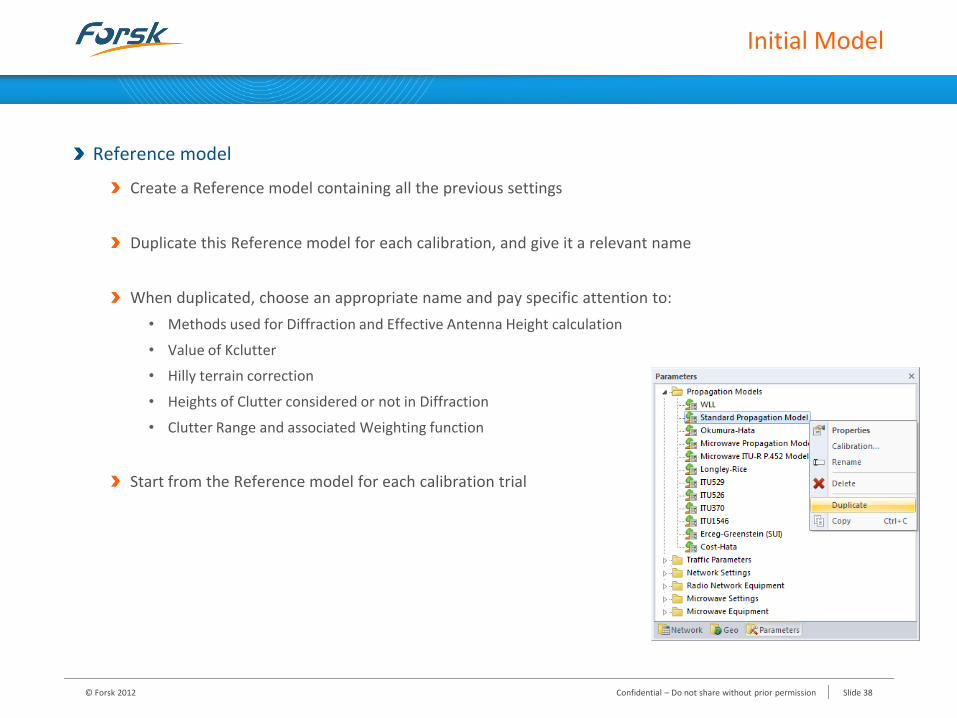
Reference model
Create a Reference model containing all the previous settings
Duplicate this Reference model for each calibration, and give it a relevant name
When duplicated, choose an appropriate name and pay specific attention to:
• Methods used for Diffraction and Effective Antenna Height calculation
• Value of Kclutter
• Hilly terrain correction
• Heights of Clutter considered or not in Diffraction
• Clutter Range and associated Weighting function
Start from the Reference model for each calibration trial
© Forsk 2012 Confidential – Do not share without prior permission Slide 38
Calibration Wizard
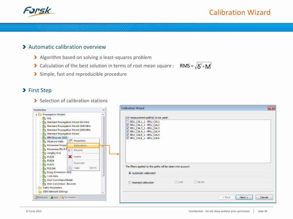
Automatic calibration overview
Algorithm based on solving a least-squares problem
Calculation of the best solution in terms of root mean square :
Simple, fast and reproducible procedure
First Step
Selection of calibration stations
Mδ22RMS
© Forsk 2012 Confidential – Do not share without prior permission Slide 39
Calibration Wizard
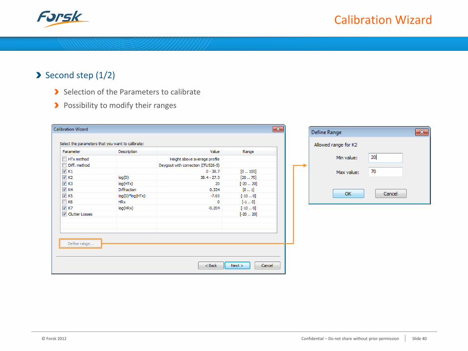
Second step (1/2)
Selection of the Parameters to calibrate
Possibility to modify their ranges
© Forsk 2012 Confidential – Do not share without prior permission Slide 40
Calibration Wizard
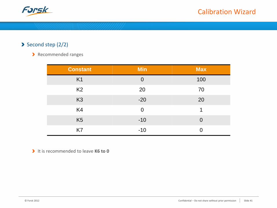
Second step (2/2)
Recommended ranges
It is recommended to leave K6 to 0
Constant Min Max
K1 0 100
K2 20 70
K3 -20 20
K4 0 1
K5 -10 0
K7 -10 0
© Forsk 2012 Confidential – Do not share without prior permission Slide 41
Calibration Wizard
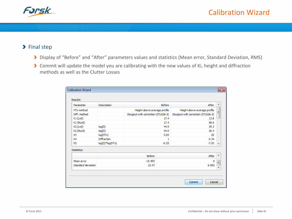
Final step
Display of “Before” and “After” parameters values and statistics (Mean error, Standard Deviation, RMS)
Commit will update the model you are calibrating with the new values of Ki, height and diffraction methods as well as the Clutter Losses
© Forsk 2012 Confidential – Do not share without prior permission Slide 42
Final Model
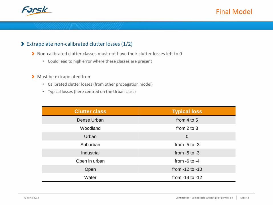
Extrapolate non-calibrated clutter losses (1/2)
Non-calibrated clutter classes must not have their clutter losses left to 0
• Could lead to high error where these classes are present
Must be extrapolated from
• Calibrated clutter losses (from other propagation model)
• Typical losses (here centred on the Urban class)
Clutter class Typical loss
Dense Urban from 4 to 5
Woodland from 2 to 3
Urban 0
Suburban from -5 to -3
Industrial from -5 to -3
Open in urban from -6 to -4
Open from -12 to -10
Water from -14 to -12
© Forsk 2012 Confidential – Do not share without prior permission Slide 43
Final Model
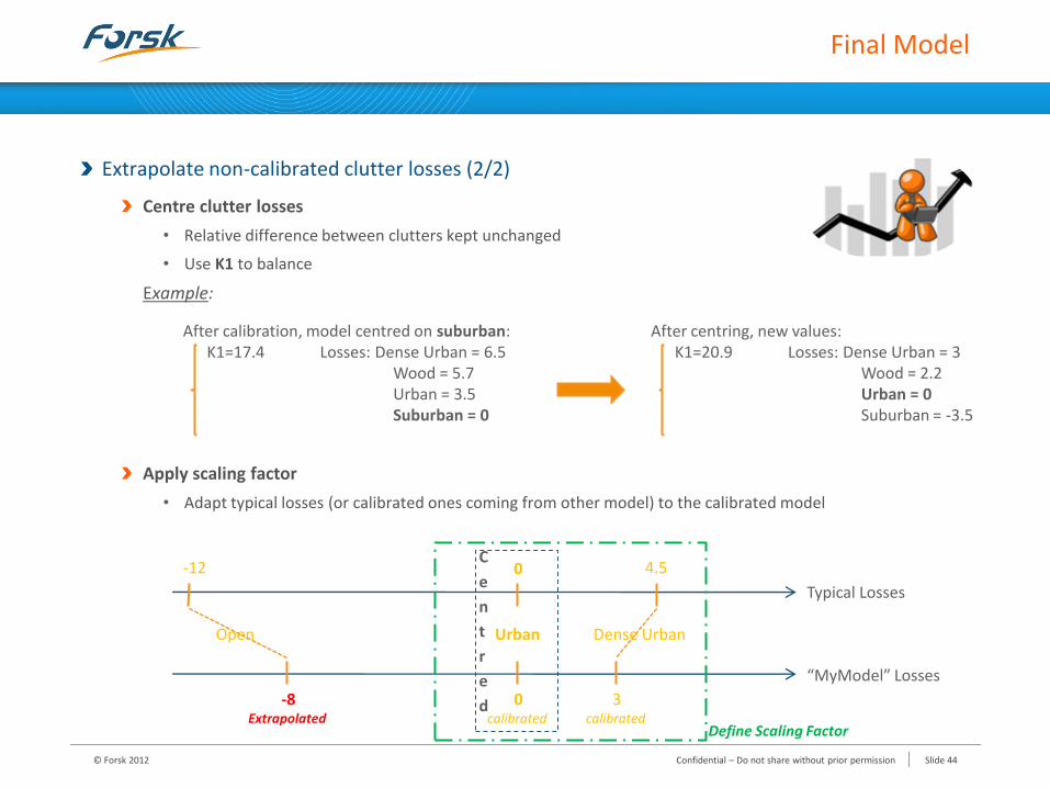
Extrapolate non-calibrated clutter losses (2/2)
Centre clutter losses
• Relative difference between clutters kept unchanged
• Use K1 to balance
Example:
Apply scaling factor
• Adapt typical losses (or calibrated ones coming from other model) to the calibrated model
After calibration, model centred on suburban: K1=17.4 Losses: Dense Urban = 6.5 Wood = 5.7 Urban = 3.5 Suburban = 0
Typical Losses
“MyModel” Losses
Urban
0
0 calibrated
4.5
3 calibrated
Dense Urban Open
-12
-8 Extrapolated
C
e
n
t
r
e
d
Define Scaling Factor
After centring, new values: K1=20.9 Losses: Dense Urban = 3 Wood = 2.2 Urban = 0 Suburban = -3.5
© Forsk 2012 Confidential – Do not share without prior permission Slide 44

1. SPM Calibration Concepts
2. Guidelines for CW Measurement Surveys
3. Working With CW Measurements
4. Automatic Calibration Method
5. Analysing the Calibrated Model
6. Calibration Process Summary
Training Programme
© Forsk 2012 Confidential – Do not share without prior permission Slide 45
5. Analysing The Calibrated Model
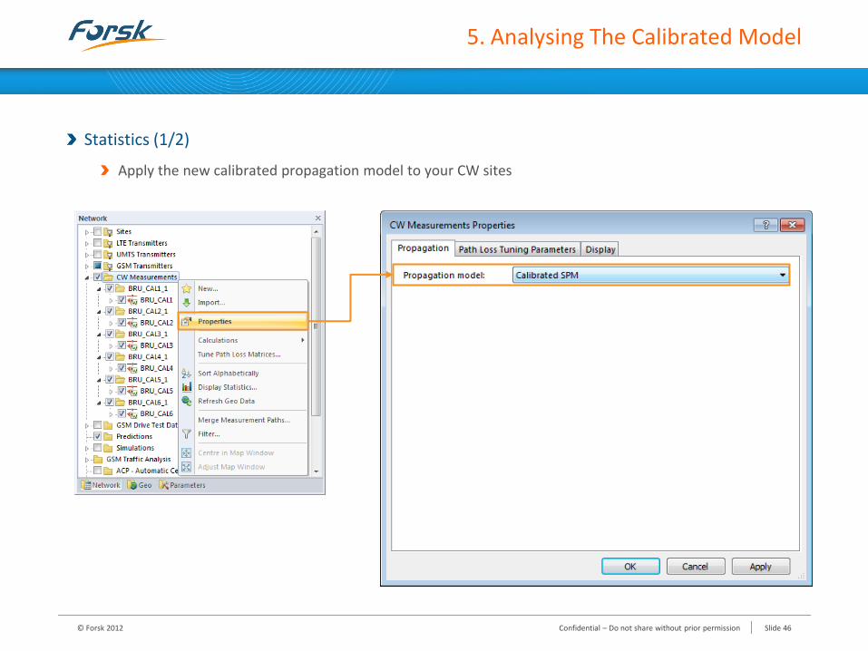
Statistics (1/2)
Apply the new calibrated propagation model to your CW sites
© Forsk 2012 Confidential – Do not share without prior permission Slide 46
5. Analysing The Calibrated Model
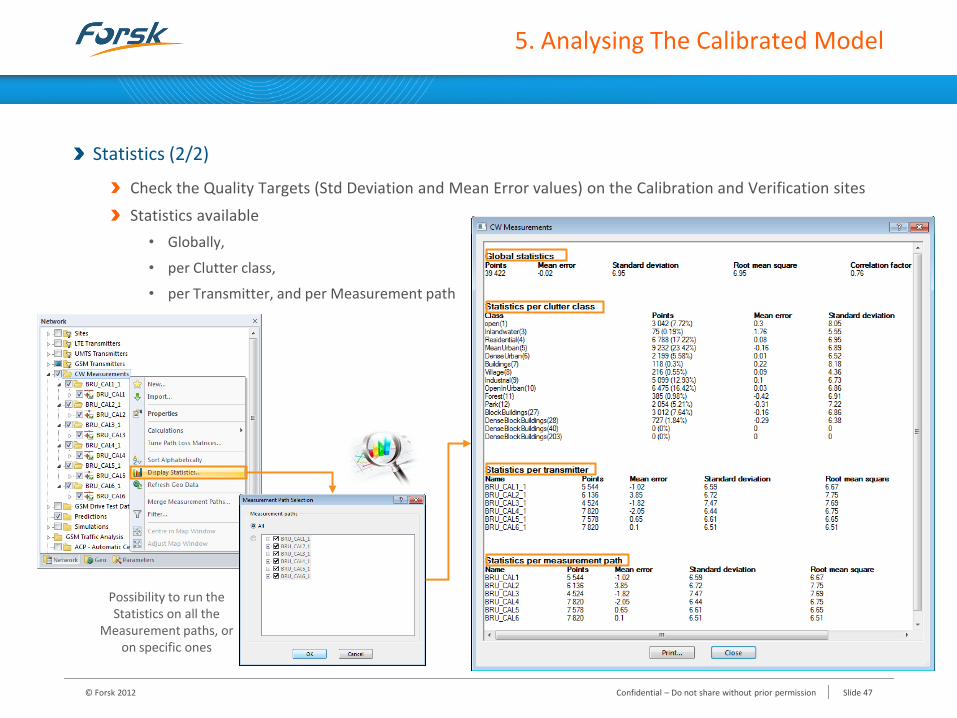
Statistics (2/2)
Check the Quality Targets (Std Deviation and Mean Error values) on the Calibration and Verification sites
Statistics available
• Globally,
• per Clutter class,
• per Transmitter, and per Measurement path
Possibility to run the Statistics on all the
Measurement paths, or on specific ones
© Forsk 2012 Confidential – Do not share without prior permission Slide 47
5. Analysing The Calibrated Model
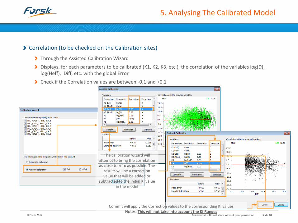
Correlation (to be checked on the Calibration sites)
Through the Assisted Calibration Wizard
Displays, for each parameters to be calibrated (K1, K2, K3, etc.), the correlation of the variables log(D), log(Heff), Diff, etc. with the global Error
Check if the Correlation values are between -0,1 and +0,1
Commit will apply the Correction values to the corresponding Ki values Notes: This will not take into account the Ki Ranges
The calibration wizard will attempt to bring the correlation as close to zero as possible. The
results will be a correction value that will be added or
subtracted to the initial Ki value in the model
© Forsk 2012 Confidential – Do not share without prior permission Slide 48
5. Analysing The Calibrated Model
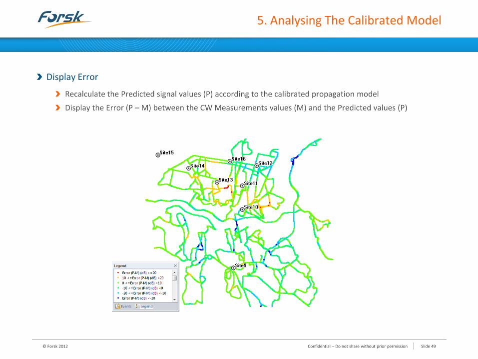
Display Error
Recalculate the Predicted signal values (P) according to the calibrated propagation model
Display the Error (P – M) between the CW Measurements values (M) and the Predicted values (P)
© Forsk 2012 Confidential – Do not share without prior permission Slide 49
5. Analysing The Calibrated Model
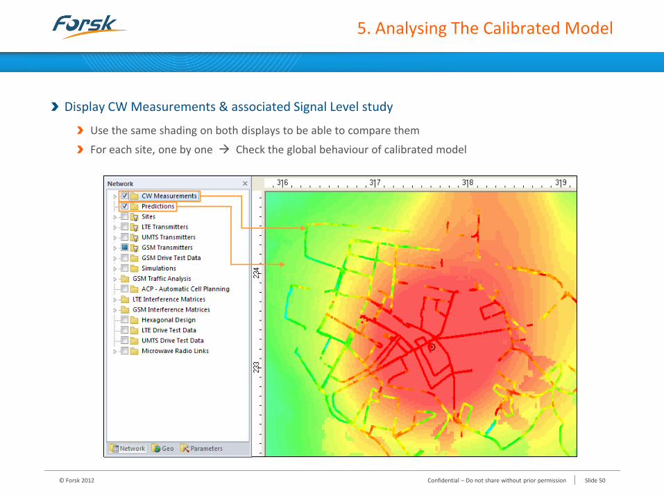
Display CW Measurements & associated Signal Level study
Use the same shading on both displays to be able to compare them
For each site, one by one Check the global behaviour of calibrated model
© Forsk 2012 Confidential – Do not share without prior permission Slide 50
5. Analysing The Calibrated Model
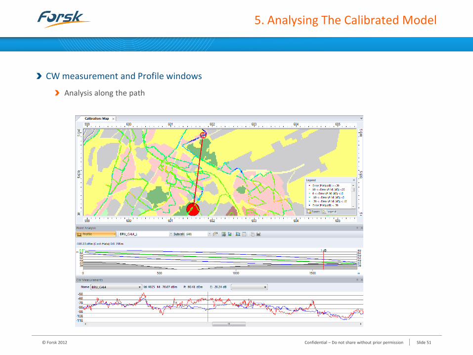
CW measurement and Profile windows
Analysis along the path
© Forsk 2012 Confidential – Do not share without prior permission Slide 51
1. SPM Calibration Concepts
2. Guidelines for CW Measurement Surveys
3. Post-process the CW Measurements Data
4. Automatic Calibration Method
5. Analysing the Calibrated Model
6. Calibration Process Summary
Training Programme
© Forsk 2012 Confidential – Do not share without prior permission Slide 52
Calibration Process Summary
Before starting...
Check Geographical Database quality & accuracy (DTM, clutter, vectors...)
Define environments (hilly, flat / urban, rural...) to specify the required number of propagation models to be calibrated
Measurements preparation
Sites selection
Survey roads
Fulfil radio criteria
Make & Average measurements
Create Transmitters used for measurements in the Atoll document
With exact configuration (coordinates, antenna type & height, EIRP, losses)
Analyse & Filter measurements ( Pre-processing)
Keep representative points and remove suspicious ones
Choice of calibration / verification sites © Forsk 2012 Confidential – Do not share without prior permission Slide 53
Calibration Process Summary
Run the automatic calibration
Display statistics and compare results with target values (Std deviation and Mean error)
for calibration sites: Global and Individual checking
for verification sites: Global checking
Extrapolate non-calibrated clutter losses
Analyse calibrated model
Display statistics
Check correlation
Maps displaying Error(P-M), Measurements & Signal Level Study, etc.
Apply the calibrated model
Apply resulting standard deviation per clutter in the clutter class description
Apply the calibrated model to network’s transmitters (Transmitter Properties\Propagation tab)
© Forsk 2012 Confidential – Do not share without prior permission Slide 54

Thank you
© Forsk 2012 Confidential – Do not share without prior permission Slide 55