Embed Size (px)
Citation preview
Atmospheric Fate and Transport of Mercury:Where does the mercury in mercury deposition come from?
Dr. Mark CohenNOAA Air Resources Laboratory
Silver Spring, Maryland, USAhttp://www.arl.noaa.gov/ss/transport/cohen.html
Presentation at the MARAMA Mercury Workshop,Cherry Hill, New Jersey, Sept 13-14, 2004
(revised version, January 2005)
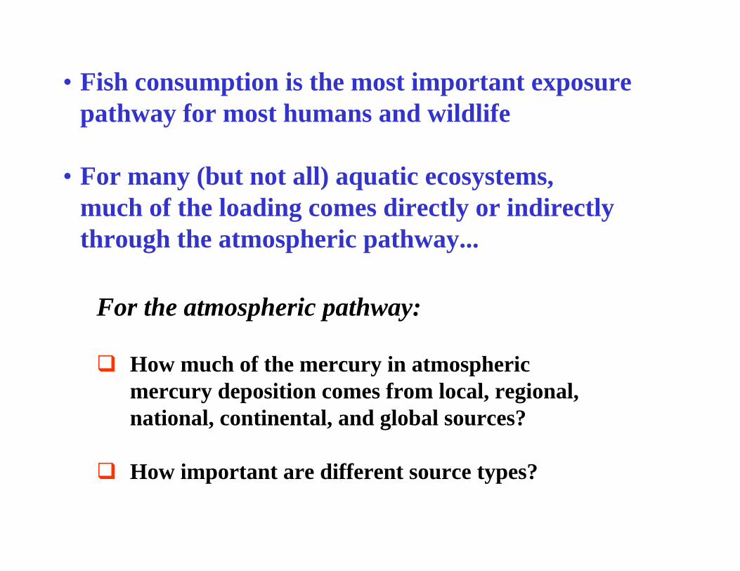
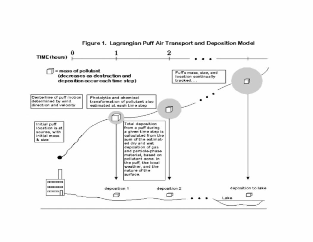
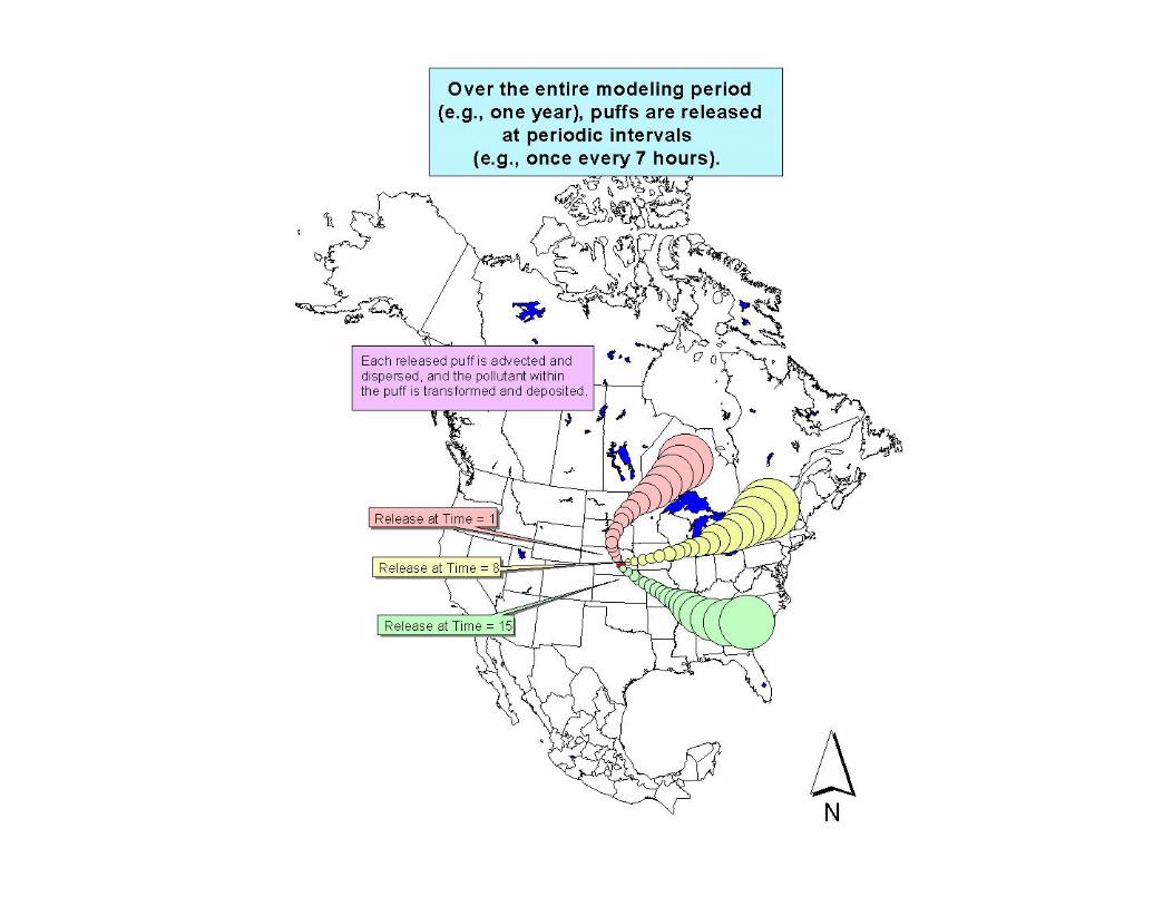
For the atmospheric pathway:
How much of the mercury in atmospheric mercury deposition comes from local, regional, national, continental, and global sources?
How important are different source types?
• Fish consumption is the most important exposure pathway for most humans and wildlife
• For many (but not all) aquatic ecosystems,much of the loading comes directly or indirectly through the atmospheric pathway...
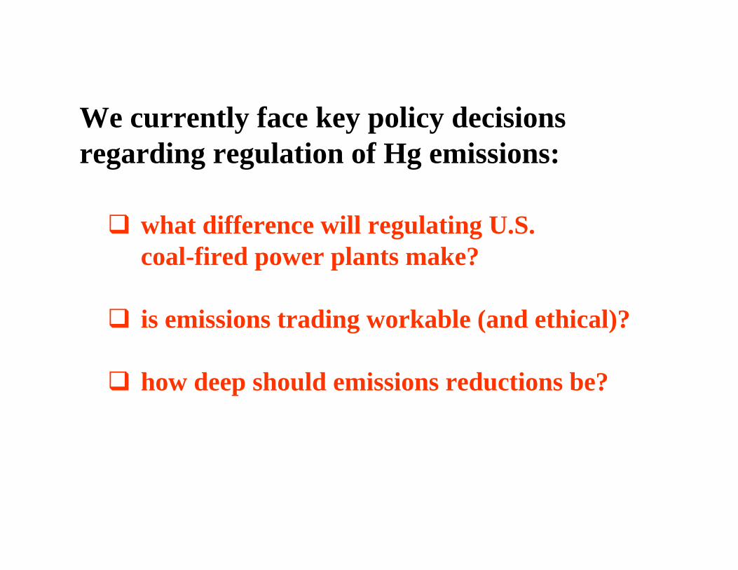
We currently face key policy decisions regarding regulation of Hg emissions:
what difference will regulating U.S. coal-fired power plants make?
is emissions trading workable (and ethical)?
how deep should emissions reductions be?
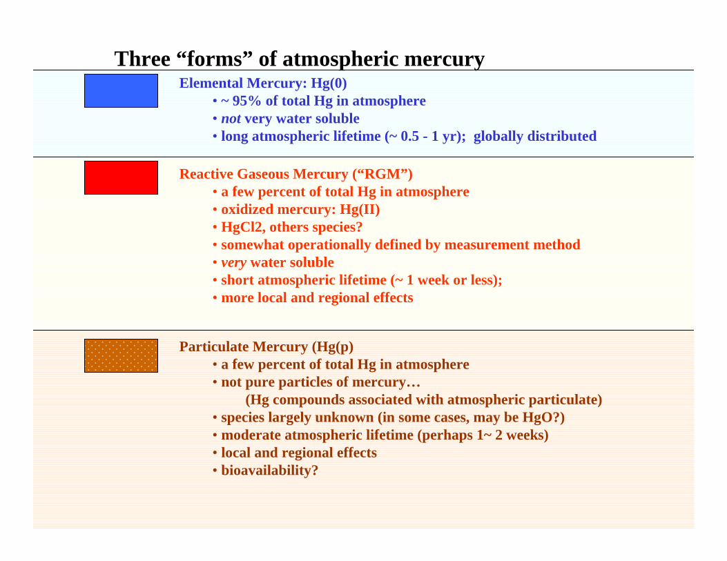
Three “forms” of atmospheric mercuryElemental Mercury: Hg(0)
• ~ 95% of total Hg in atmosphere• not very water soluble• long atmospheric lifetime (~ 0.5 - 1 yr); globally distributed
Reactive Gaseous Mercury (“RGM”)• a few percent of total Hg in atmosphere• oxidized mercury: Hg(II)• HgCl2, others species?• somewhat operationally defined by measurement method• very water soluble• short atmospheric lifetime (~ 1 week or less);• more local and regional effects
Particulate Mercury (Hg(p)• a few percent of total Hg in atmosphere• not pure particles of mercury…
(Hg compounds associated with atmospheric particulate)• species largely unknown (in some cases, may be HgO?)• moderate atmospheric lifetime (perhaps 1~ 2 weeks)• local and regional effects• bioavailability?
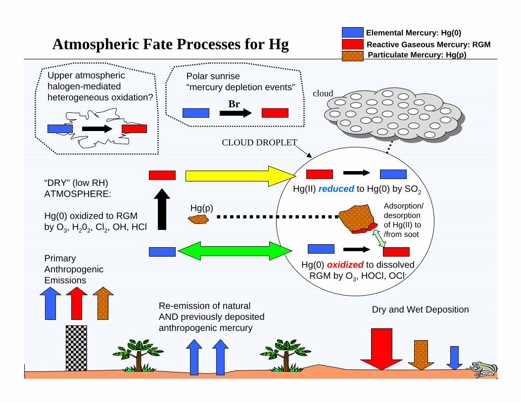
CLOUD DROPLET
cloud
PrimaryAnthropogenicEmissions
Reactive Gaseous Mercury: RGMElemental Mercury: Hg(0)
Particulate Mercury: Hg(p)Atmospheric Fate Processes for Hg
Dry and Wet Deposition
Hg(0) oxidized to dissolvedRGM by O3, HOCl, OCl-
Hg(II) reduced to Hg(0) by SO2
Re-emission of natural AND previously depositedanthropogenic mercury
Adsorption/desorptionof Hg(II) to/from soot
Hg(p)
“DRY” (low RH)ATMOSPHERE:
Hg(0) oxidized to RGMby O3, H202, Cl2, OH, HCl
Polar sunrise“mercury depletion events”
Br
Upper atmospherichalogen-mediatedheterogeneous oxidation?
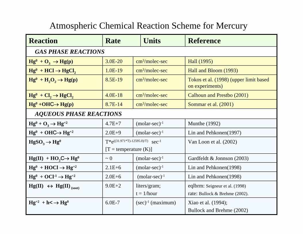
GAS PHASE REACTIONS
AQUEOUS PHASE REACTIONS
ReferenceUnitsRateReaction
Xiao et al. (1994); Bullock and Brehme (2002)
(sec)-1 (maximum)6.0E-7Hg+2 + h<→ Hg0
eqlbrm: Seigneur et al. (1998)
rate: Bullock & Brehme (2002).
liters/gram;t = 1/hour
9.0E+2Hg(II) ↔ Hg(II) (soot)
Lin and Pehkonen(1998)(molar-sec)-12.0E+6Hg0 + OCl-1 → Hg+2
Lin and Pehkonen(1998)(molar-sec)-12.1E+6Hg0 + HOCl → Hg+2
Gardfeldt & Jonnson (2003)(molar-sec)-1~ 0Hg(II) + HO2C→ Hg0
Van Loon et al. (2002)T*e((31.971*T)-12595.0)/T) sec-1
[T = temperature (K)]HgSO3 → Hg0
Lin and Pehkonen(1997)(molar-sec)-12.0E+9Hg0 + OHC→ Hg+2
Munthe (1992)(molar-sec)-14.7E+7Hg0 + O3 → Hg+2
Sommar et al. (2001)cm3/molec-sec8.7E-14Hg0 +OHC→ Hg(p)
Calhoun and Prestbo (2001)cm3/molec-sec4.0E-18Hg0 + Cl2 → HgCl2
Tokos et al. (1998) (upper limit based on experiments)
cm3/molec-sec8.5E-19Hg0 + H2O2 → Hg(p)
Hall and Bloom (1993)cm3/molec-sec1.0E-19Hg0 + HCl → HgCl2
Hall (1995)cm3/molec-sec3.0E-20Hg0 + O3 → Hg(p)
Atmospheric Chemical Reaction Scheme for Mercury
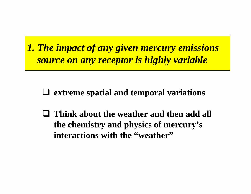
1. The impact of any given mercury emissions source on any receptor is highly variable
extreme spatial and temporal variations
Think about the weather and then add all the chemistry and physics of mercury’s interactions with the “weather”
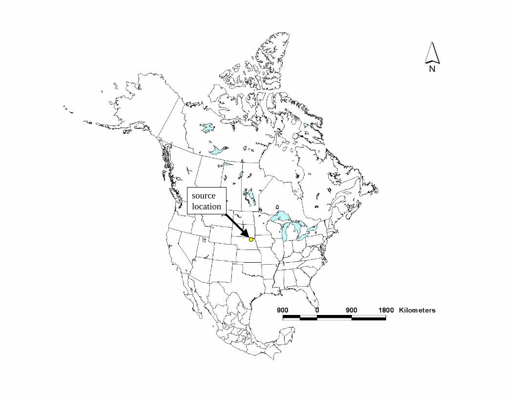
sourcelocation
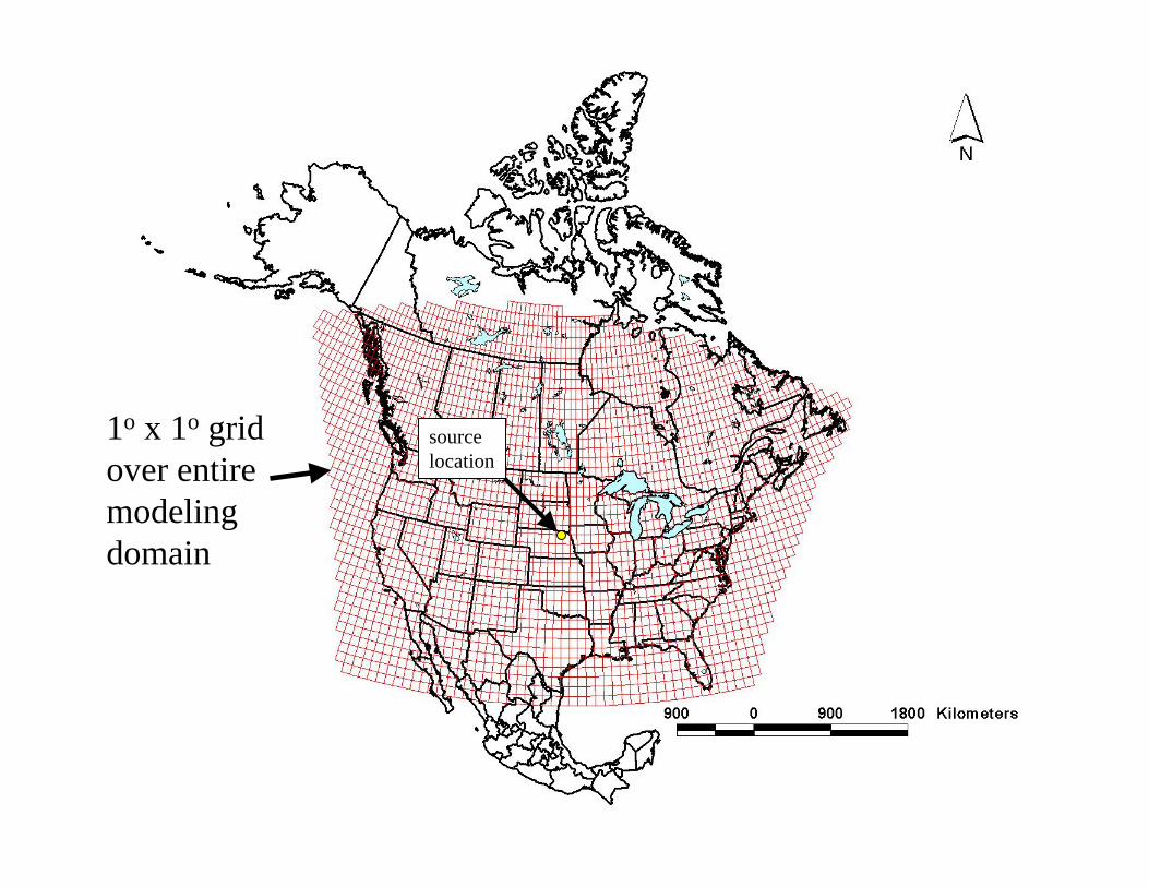
1o x 1o grid over entire modeling domain
sourcelocation
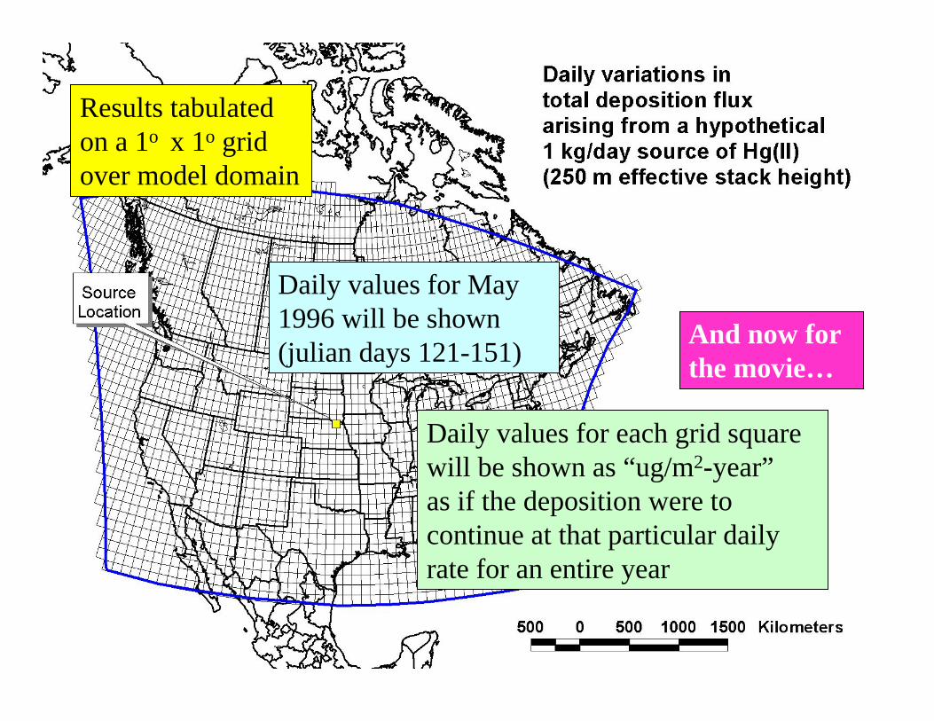
Results tabulated on a 1o x 1o gridover model domain
Daily values for each grid square will be shown as “ug/m2-year”as if the deposition were to continue at that particular daily rate for an entire year
Daily values for May 1996 will be shown (julian days 121-151) And now for
the movie…
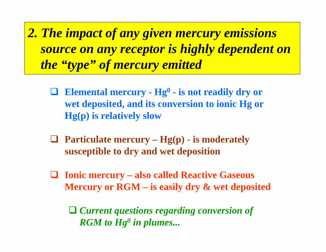
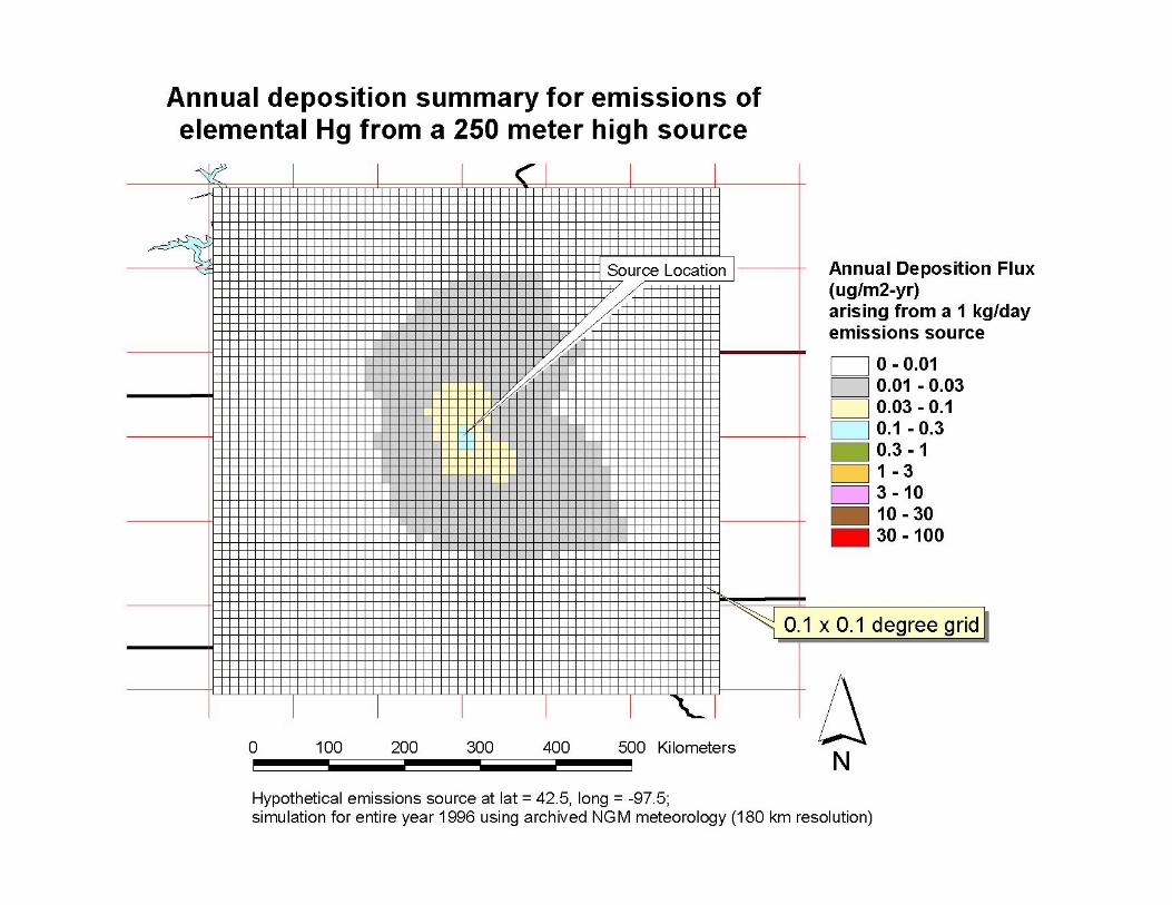
2. The impact of any given mercury emissions source on any receptor is highly dependent on the “type” of mercury emitted
Elemental mercury - Hg0 - is not readily dry or wet deposited, and its conversion to ionic Hg or Hg(p) is relatively slow
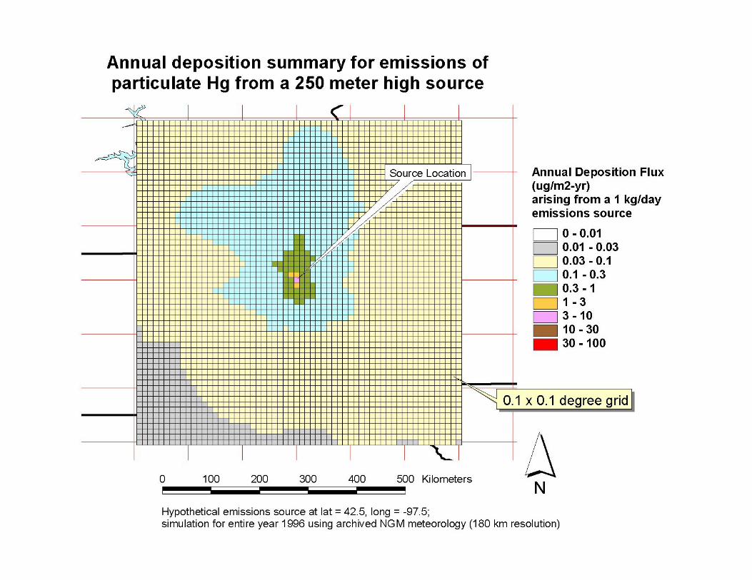
Particulate mercury – Hg(p) - is moderately susceptible to dry and wet deposition
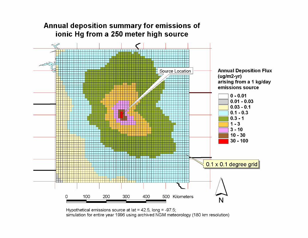
Ionic mercury – also called Reactive Gaseous Mercury or RGM – is easily dry & wet deposited
Current questions regarding conversion of RGM to Hg0 in plumes...
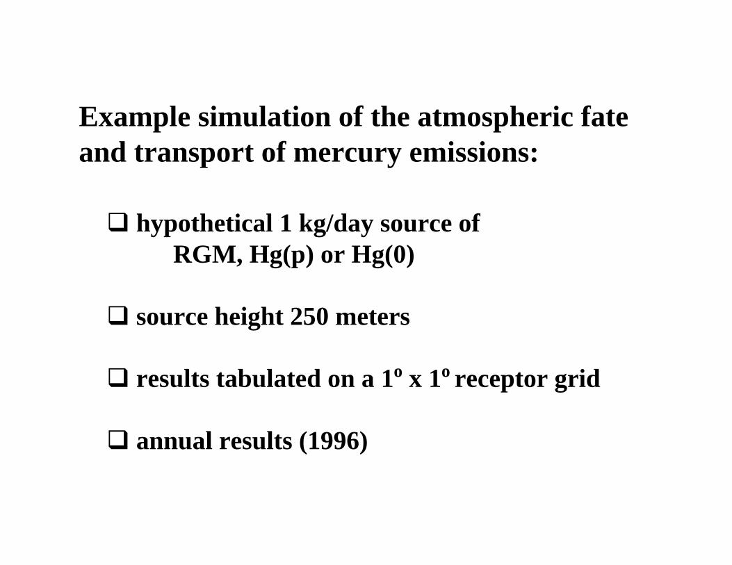
Example simulation of the atmospheric fate and transport of mercury emissions:
hypothetical 1 kg/day source of RGM, Hg(p) or Hg(0)
source height 250 meters
results tabulated on a 1o x 1o receptor grid
annual results (1996)
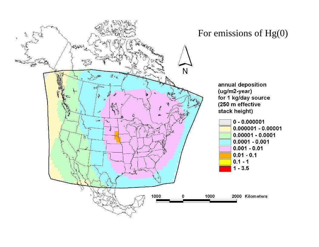
For emissions of Hg(0)
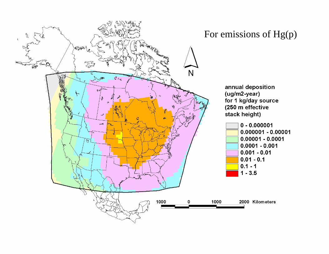
For emissions of Hg(p)
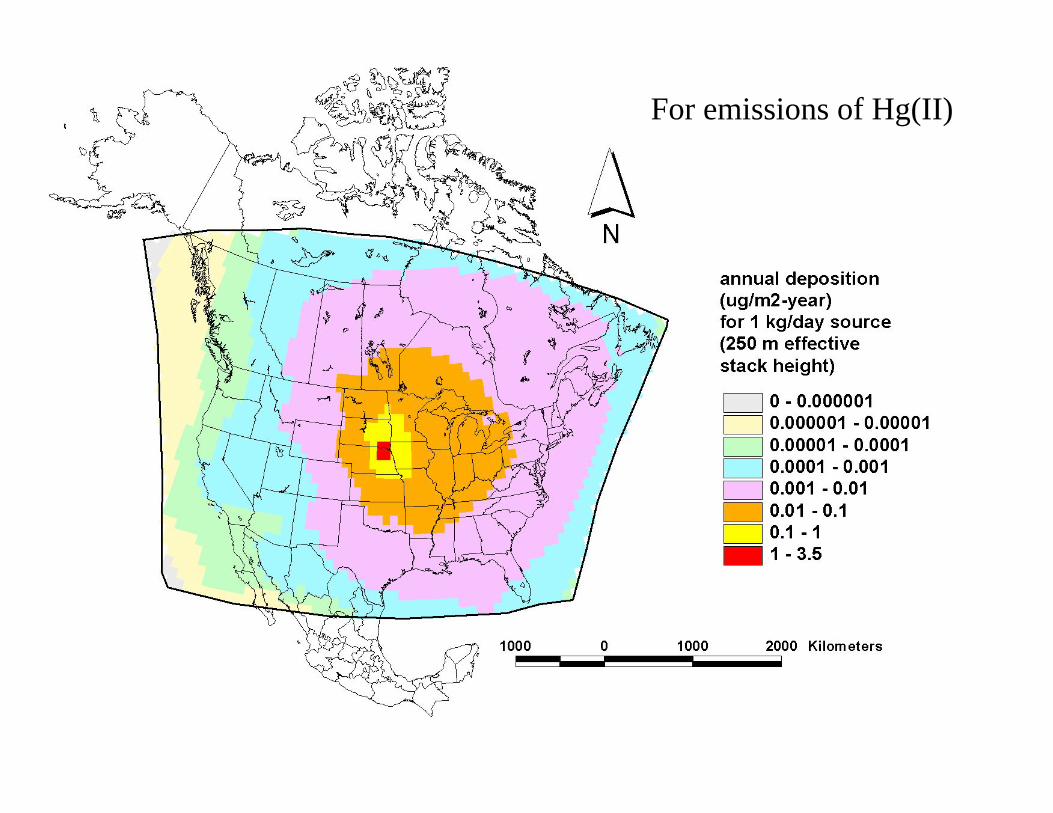
For emissions of Hg(II)
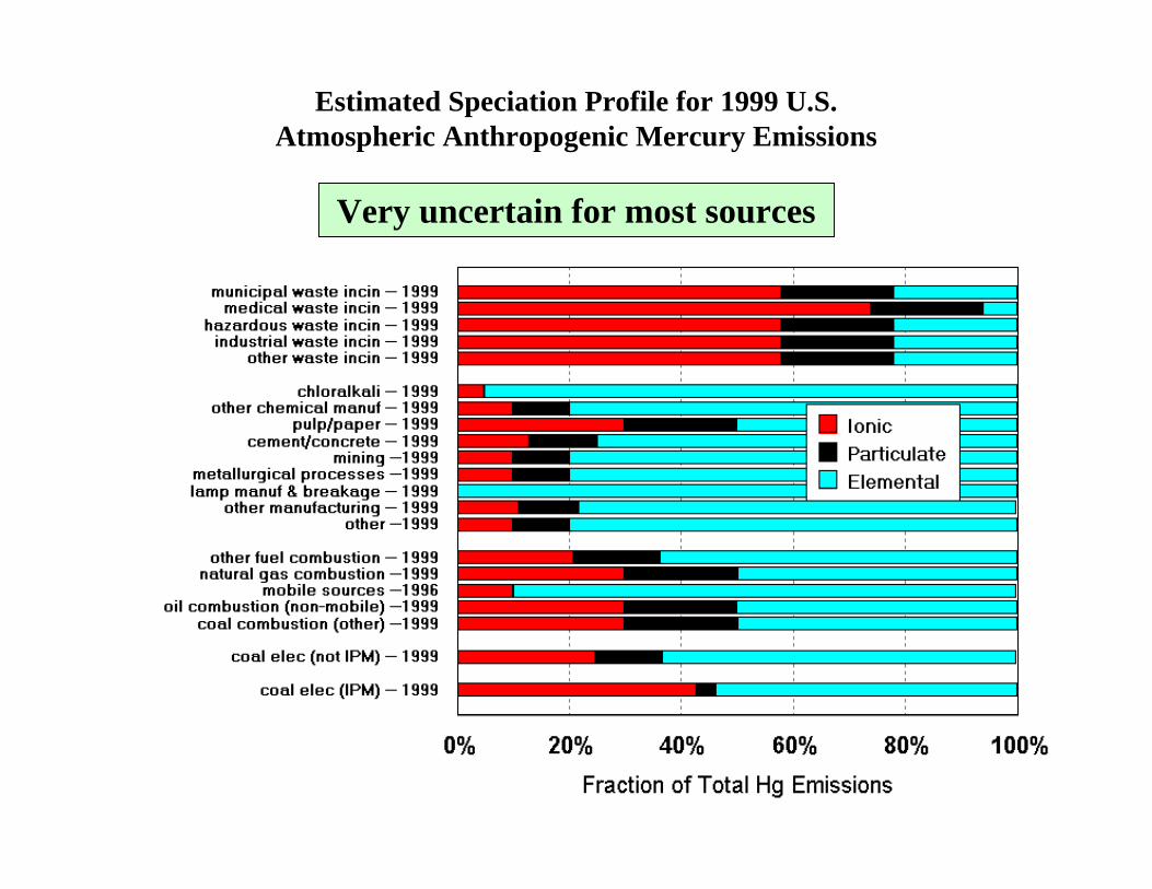
Estimated Speciation Profile for 1999 U.S.Atmospheric Anthropogenic Mercury Emissions
Very uncertain for most sources
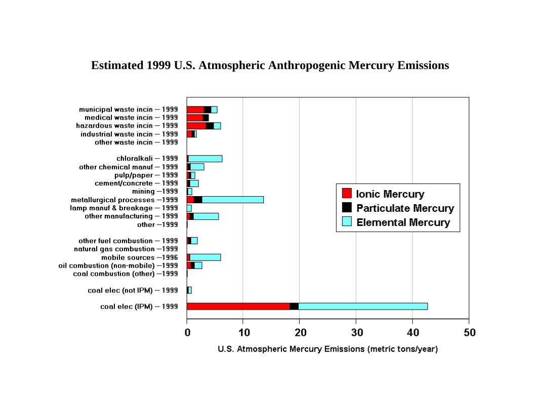
Estimated 1999 U.S. Atmospheric Anthropogenic Mercury Emissions
Each type of source has a very different emissions speciation profile
Even within a given source type, there can be big differences – depending on process type, fuels and raw materials, pollution control equipment, etc.
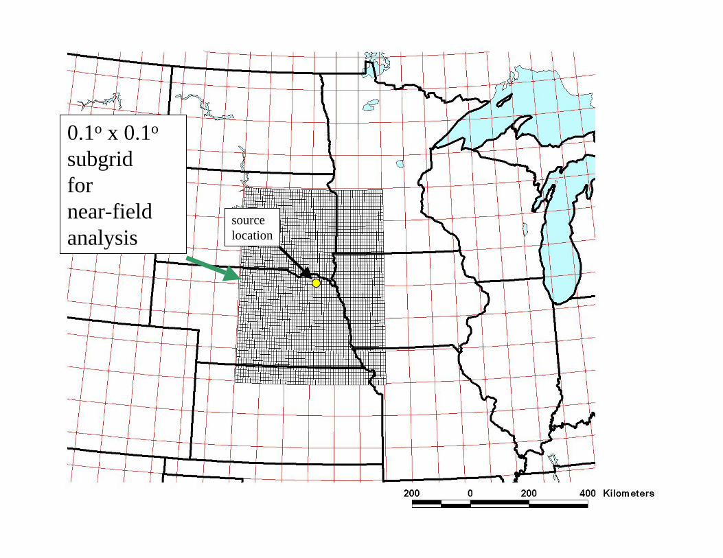
3. There can be large local and regional impacts from any given source
same hypothetical 1 kg/day source of RGM
source height 250 meters
exactly the same simulation, but results tabulated on a 0.1o x 0.1o receptor grid
overall results for an entire year (1996)
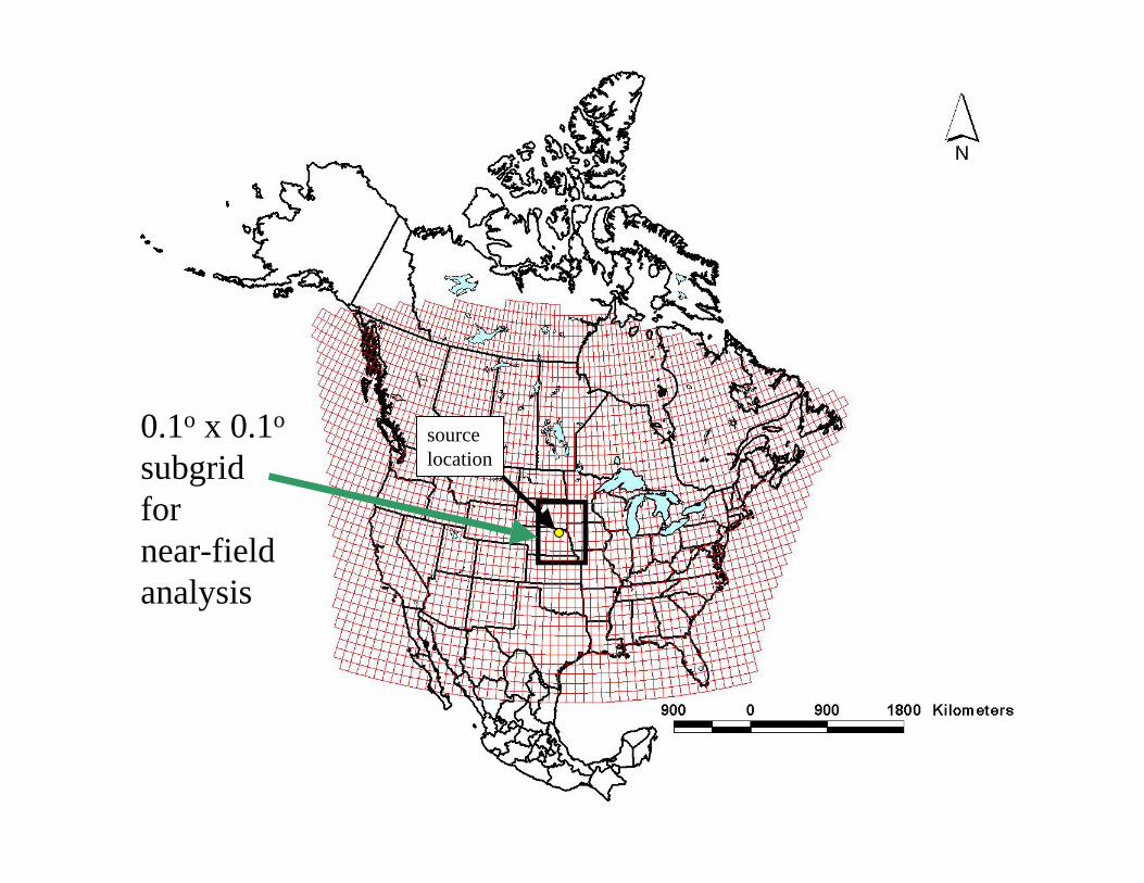
0.1o x 0.1o
subgrid for near-field analysis
sourcelocation
0.1o x 0.1o
subgrid for near-field analysis
sourcelocation
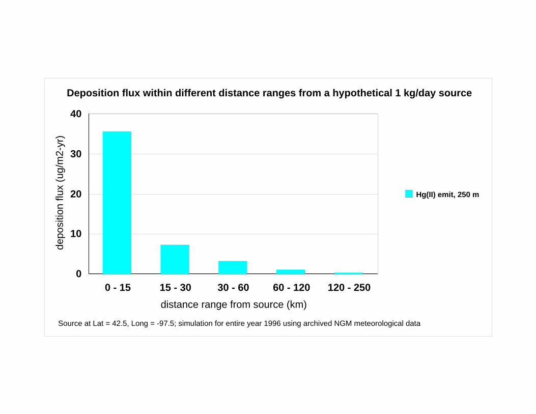
0 - 15 15 - 30 30 - 60 60 - 120 120 - 250distance range from source (km)
0
10
20
30
40
depo
sitio
n flu
x (u
g/m
2-yr
)
Hg(II) emit, 250 m
Source at Lat = 42.5, Long = -97.5; simulation for entire year 1996 using archived NGM meteorological data
Deposition flux within different distance ranges from a hypothetical 1 kg/day source
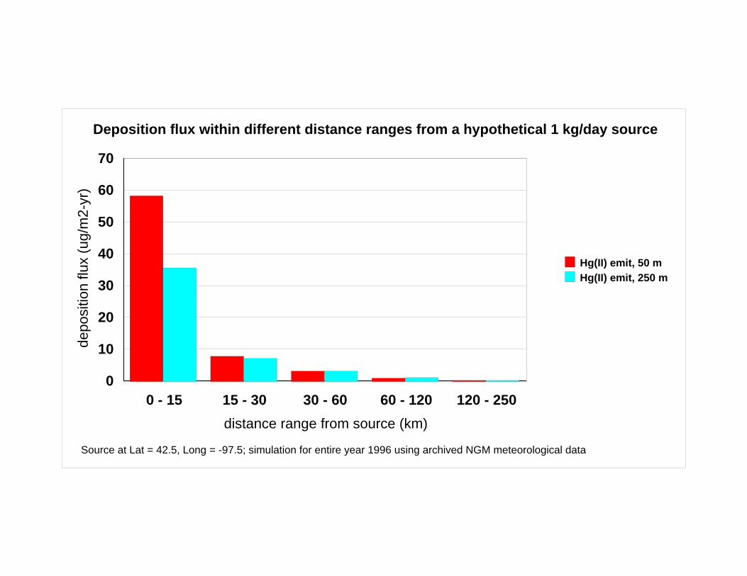
0 - 15 15 - 30 30 - 60 60 - 120 120 - 250distance range from source (km)
0
10
20
30
40
50
60
70
depo
sitio
n flu
x (u
g/m
2-yr
)
Hg(II) emit, 50 mHg(II) emit, 250 m
Source at Lat = 42.5, Long = -97.5; simulation for entire year 1996 using archived NGM meteorological data
Deposition flux within different distance ranges from a hypothetical 1 kg/day source
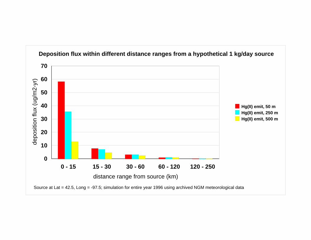
0 - 15 15 - 30 30 - 60 60 - 120 120 - 250distance range from source (km)
0
10
20
30
40
50
60
70
depo
sitio
n flu
x (u
g/m
2-yr
)
Hg(II) emit, 50 mHg(II) emit, 250 mHg(II) emit, 500 m
Source at Lat = 42.5, Long = -97.5; simulation for entire year 1996 using archived NGM meteorological data
Deposition flux within different distance ranges from a hypothetical 1 kg/day source
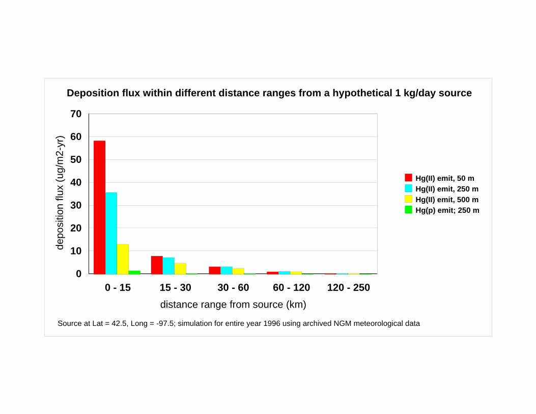
0 - 15 15 - 30 30 - 60 60 - 120 120 - 250distance range from source (km)
0
10
20
30
40
50
60
70
depo
sitio
n flu
x (u
g/m
2-yr
)
Hg(II) emit, 50 mHg(II) emit, 250 mHg(II) emit, 500 mHg(p) emit; 250 m
Source at Lat = 42.5, Long = -97.5; simulation for entire year 1996 using archived NGM meteorological data
Deposition flux within different distance ranges from a hypothetical 1 kg/day source
0 - 15 15 - 30 30 - 60 60 - 120 120 - 250distance range from source (km)
0.001
0.01
0.1
1
10
100
depo
sitio
n flu
x (u
g/m
2-yr
)
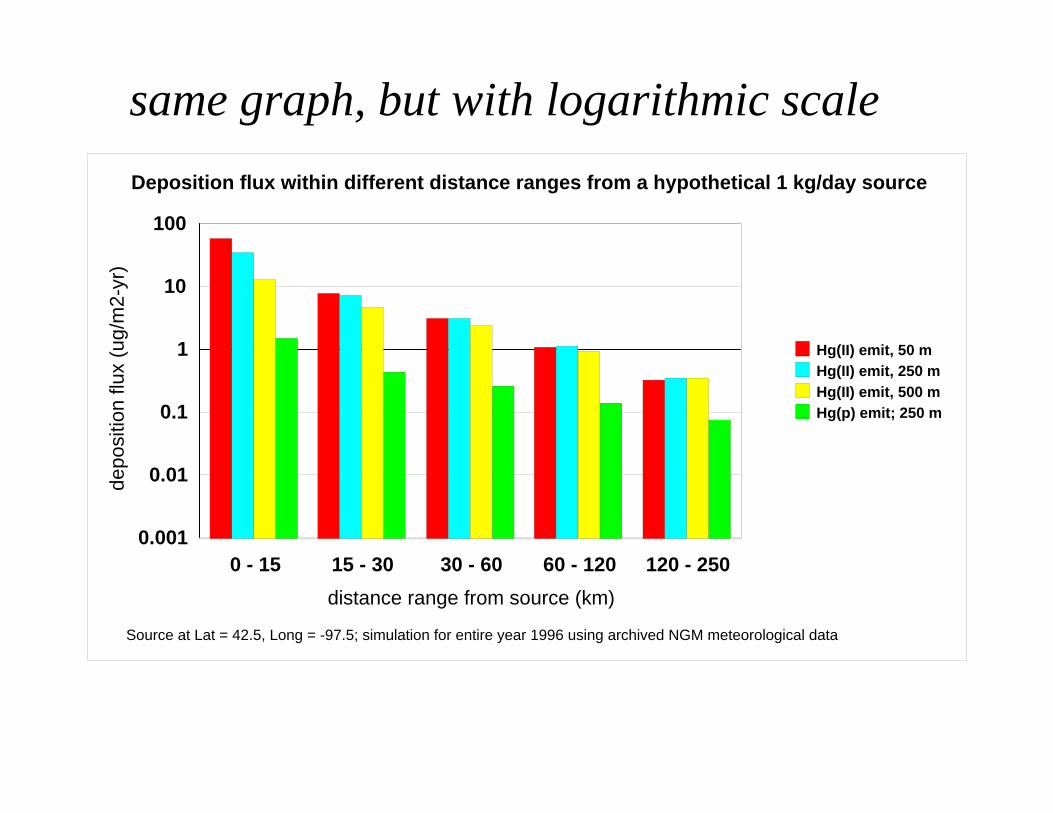
Hg(II) emit, 50 mHg(II) emit, 250 mHg(II) emit, 500 mHg(p) emit; 250 m
Source at Lat = 42.5, Long = -97.5; simulation for entire year 1996 using archived NGM meteorological data
Deposition flux within different distance ranges from a hypothetical 1 kg/day source
same graph, but with logarithmic scale
0 - 15 15 - 30 30 - 60 60 - 120 120 - 250distance range from source (km)
0.001
0.01
0.1
1
10
100
depo
sitio
n flu
x (u
g/m
2-yr
)
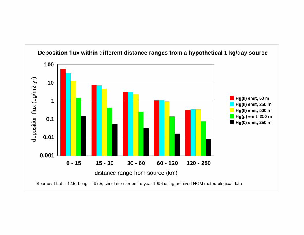
Hg(II) emit, 50 mHg(II) emit, 250 mHg(II) emit, 500 mHg(p) emit; 250 mHg(0) emit, 250 m
Source at Lat = 42.5, Long = -97.5; simulation for entire year 1996 using archived NGM meteorological data
Deposition flux within different distance ranges from a hypothetical 1 kg/day source
4. At the same time, medium to long range transport can’t be ignored
15 30 60 120 250 500 750 1000 1250 1500 1750 2000 2250 2500
distance range from source (km)
0.001
0.01
0.1
1
cum
ulat
ive
fract
ion
depo
site
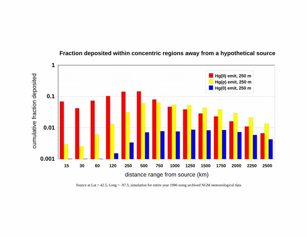
d Hg(II) emit, 250 mHg(p) emit, 250 mHg(0) emit, 250 m
Source at Lat = 42.5, Long = -97.5; simulation for entire year 1996 using archived NGM meteorological data
Fraction deposited within concentric regions away from a hypothetical source
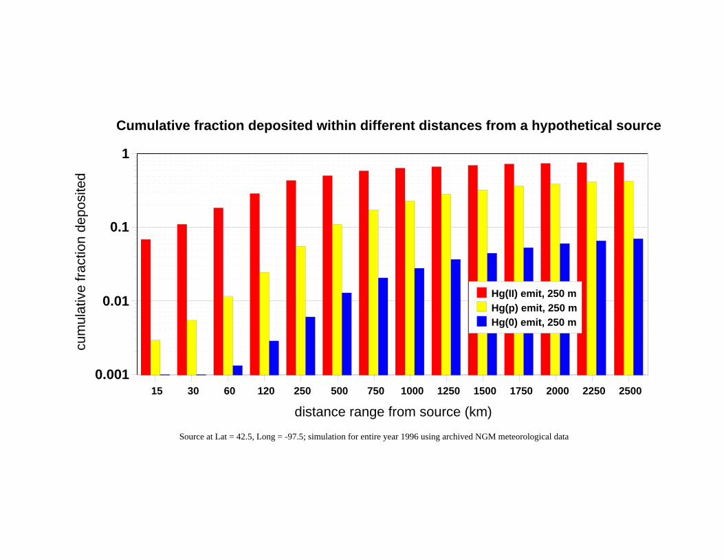
15 30 60 120 250 500 750 1000 1250 1500 1750 2000 2250 2500
distance range from source (km)
0.001
0.01
0.1
1
cum
ulat
ive
fract
ion
depo
site
d
Hg(II) emit, 250 mHg(p) emit, 250 mHg(0) emit, 250 m
Source at Lat = 42.5, Long = -97.5; simulation for entire year 1996 using archived NGM meteorological data
Cumulative fraction deposited within different distances from a hypothetical source
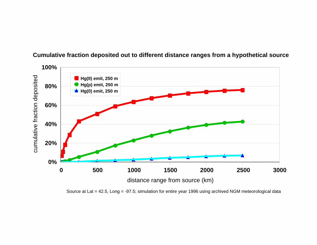
0 500 1000 1500 2000 2500 3000distance range from source (km)
0%
20%
40%
60%
80%
100%
cum
ulat
ive
fract
ion
depo
site
d Hg(II) emit, 250 mHg(p) emit, 250 mHg(0) emit, 250 m
Source at Lat = 42.5, Long = -97.5; simulation for entire year 1996 using archived NGM meteorological data
Cumulative fraction deposited out to different distance ranges from a hypothetical source
0 500 1000 1500 2000 2500 3000distance range from source (km)
0%
20%
40%
60%
80%
100%
cum
ulat
ive
fract
ion
depo
site
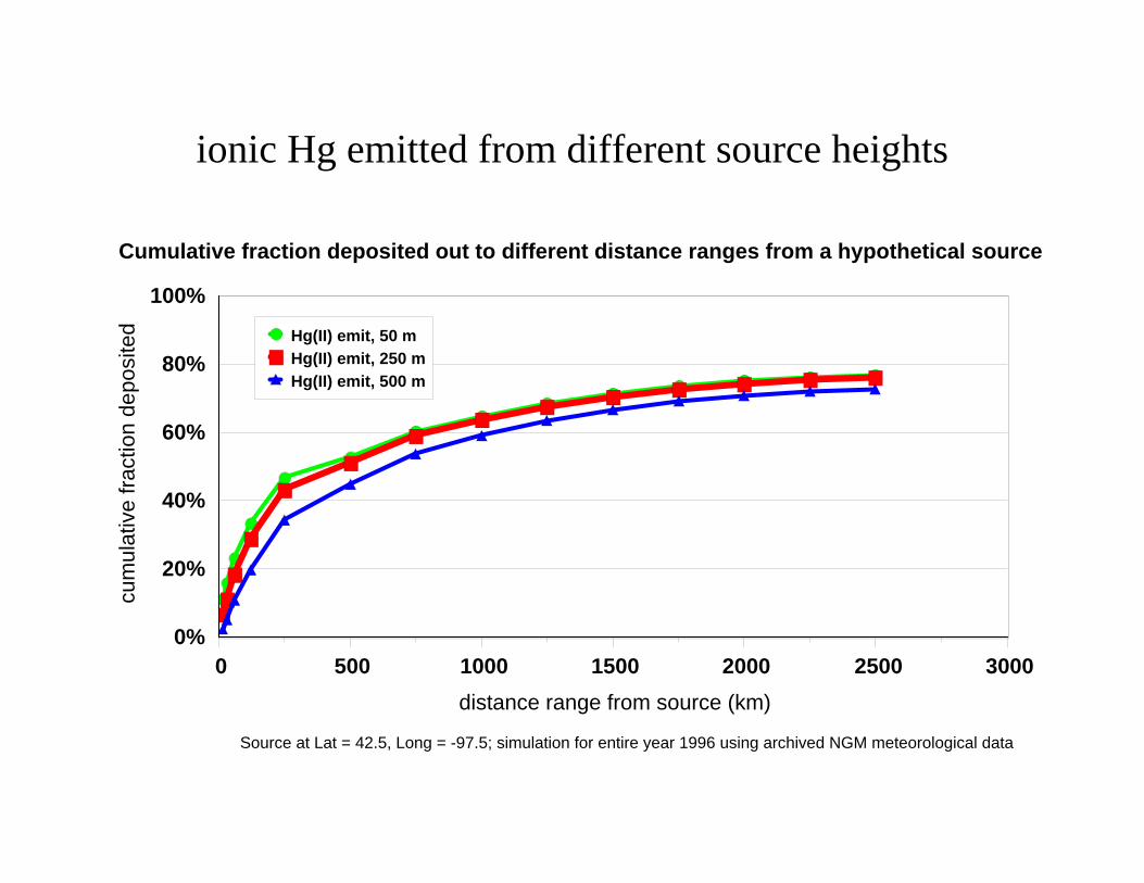
d Hg(II) emit, 50 mHg(II) emit, 250 mHg(II) emit, 500 m
Source at Lat = 42.5, Long = -97.5; simulation for entire year 1996 using archived NGM meteorological data
Cumulative fraction deposited out to different distance ranges from a hypothetical source
ionic Hg emitted from different source heights
0 500 1000 1500 2000 2500 3000distance range from source (km)
0%
10%
20%
30%
40%
50%
cum
ulat
ive
fract
ion
depo
site
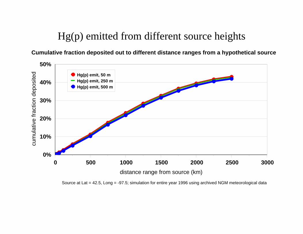
d Hg(p) emit, 50 mHg(p) emit, 250 mHg(p) emit, 500 m
Source at Lat = 42.5, Long = -97.5; simulation for entire year 1996 using archived NGM meteorological data
Cumulative fraction deposited out to different distance ranges from a hypothetical source
Hg(p) emitted from different source heights
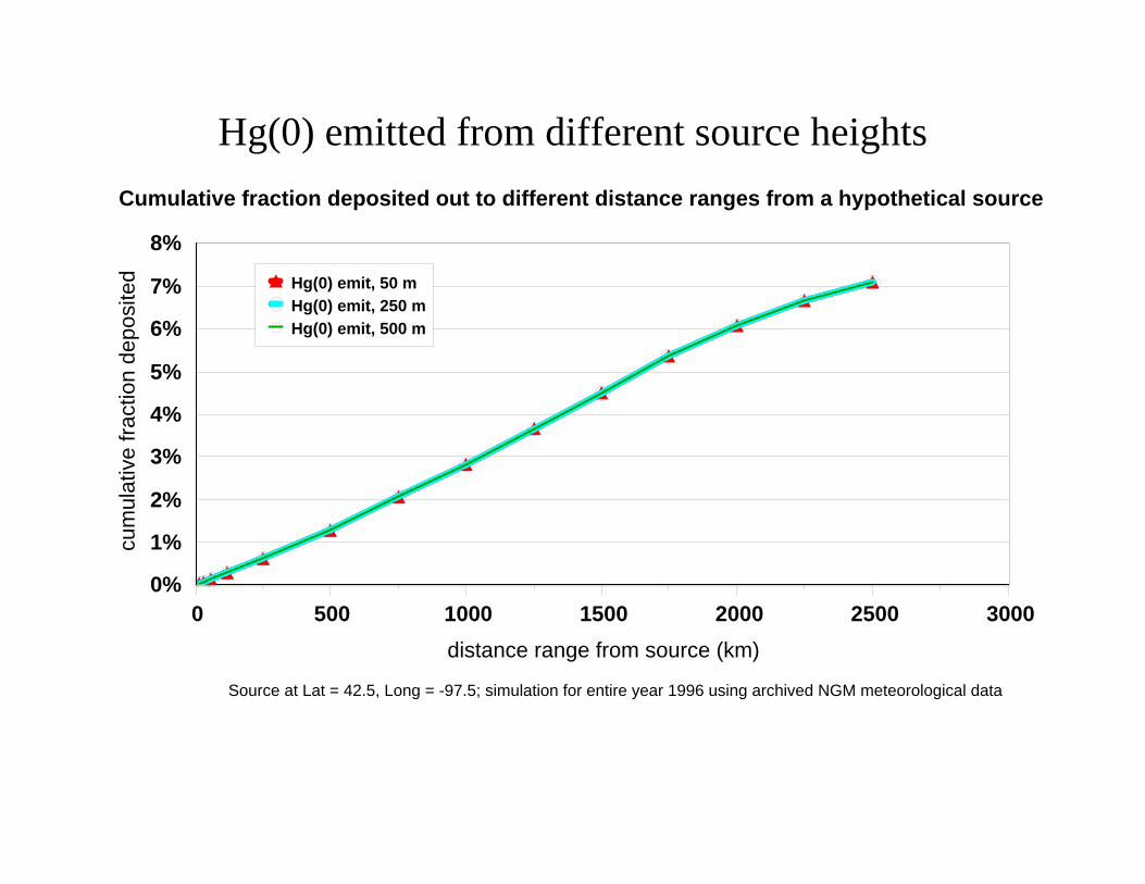
0 500 1000 1500 2000 2500 3000distance range from source (km)
0%
1%
2%
3%
4%
5%
6%
7%
8%
cum
ulat
ive
fract
ion
depo
site
d Hg(0) emit, 50 mHg(0) emit, 250 mHg(0) emit, 500 m
Source at Lat = 42.5, Long = -97.5; simulation for entire year 1996 using archived NGM meteorological data
Cumulative fraction deposited out to different distance ranges from a hypothetical source
Hg(0) emitted from different source heights
5. There are a lot of sources…
Large spatial and temporal variations
Each source emits mercury forms in different proportions
A lot of different sources can contribute significant amounts of mercury through atmospheric deposition to any given receptor
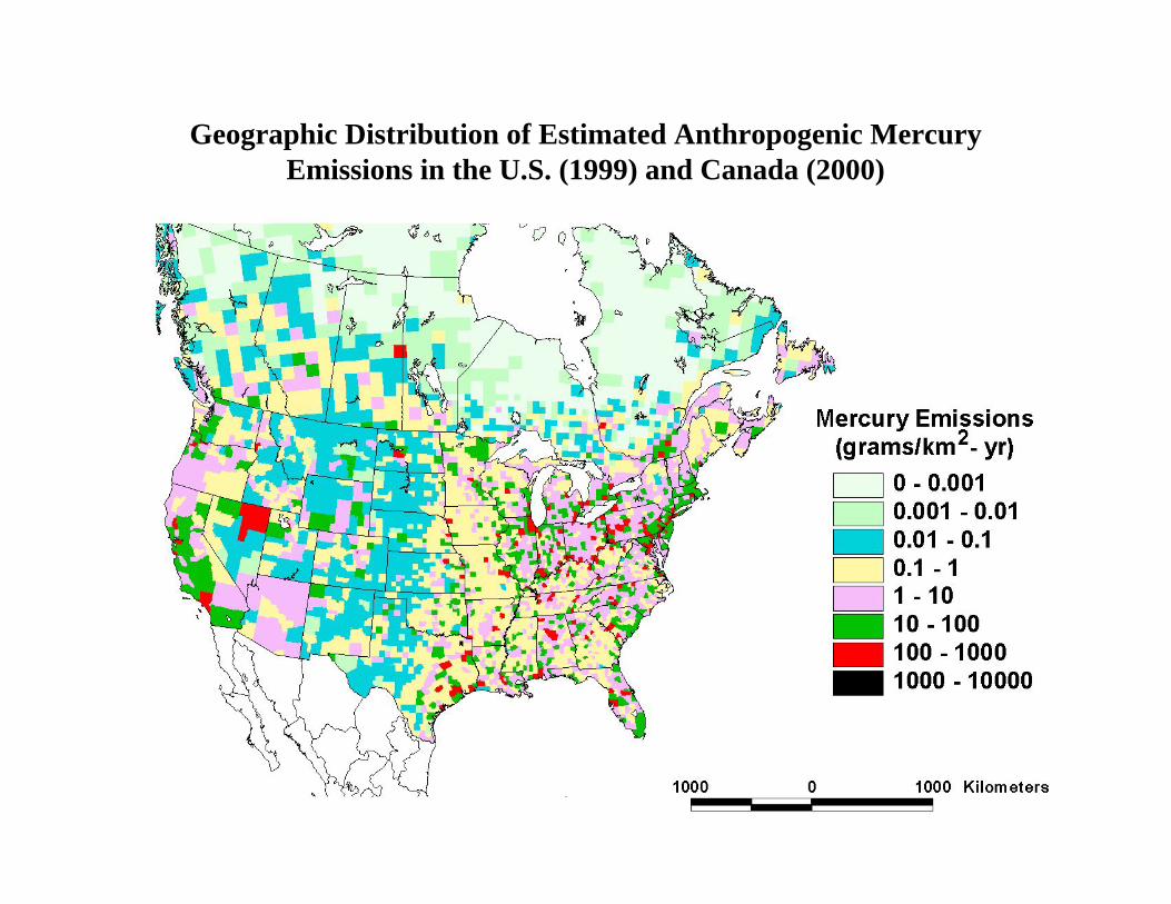
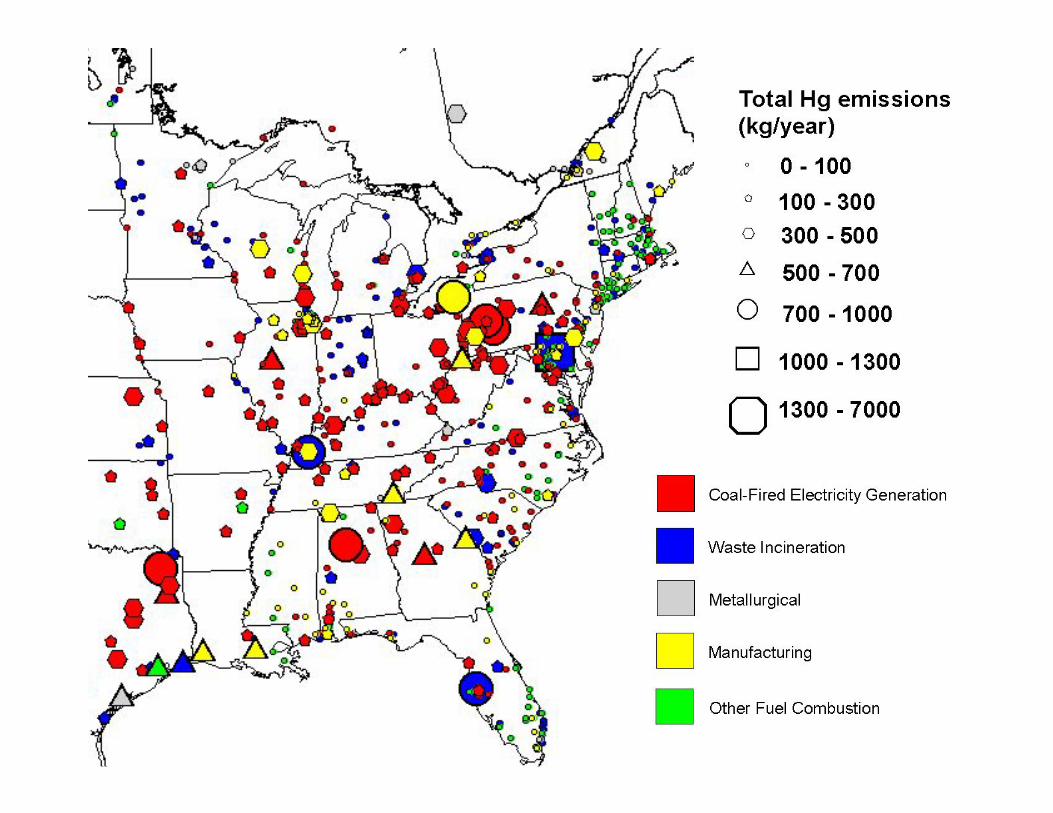
Geographic Distribution of Estimated Anthropogenic Mercury Emissions in the U.S. (1999) and Canada (2000)
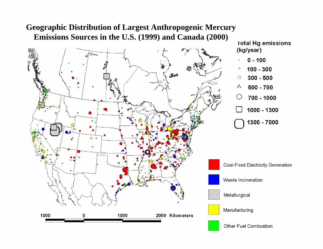
Geographic Distribution of Largest Anthropogenic Mercury Emissions Sources in the U.S. (1999) and Canada (2000)
6. Getting the source-apportionment information we all need is difficult
With measurements alone, generally impossible
Coupling measurements with back-trajectory analyses yields only a little information
Comprehensive fate and transport modeling –“forward” from emissions to deposition – holds the promise of generating detailed source-receptor information
Statescan playa key rolein these
7. There are a lot of uncertainties in current comprehensive fate and transport models
atmospheric chemistry of mercury
concentrations of key reactants
meteorological data (e.g., precipitation)
mercury emissions (amounts & speciation profile)
data for evaluation are scarce...
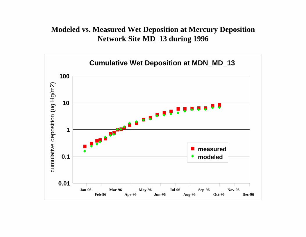
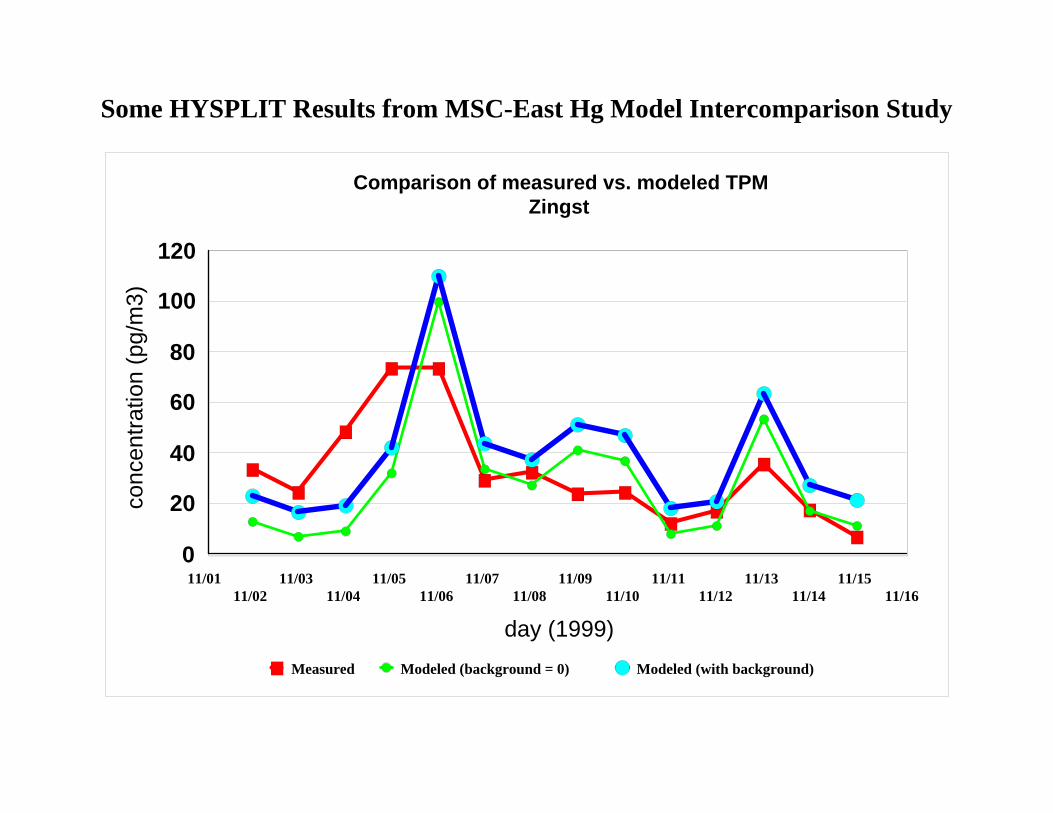
8. Nevertheless, many models seem to be performing reasonably well, i.e., are able to explain a lot of what we see
Jan-96Feb-96
Mar-96Apr-96
May-96Jun-96
Jul-96Aug-96
Sep-96Oct-96
Nov-96Dec-96
0.01
0.1
1
10
100
cum
ulat
ive
depo
sitio
n (u
g H
g/m
2)
measuredmodeled
Cumulative Wet Deposition at MDN_MD_13
Modeled vs. Measured Wet Deposition at Mercury Deposition Network Site MD_13 during 1996
11/0111/02
11/0311/04
11/0511/06
11/0711/08
11/0911/10
11/1111/12
11/1311/14
11/1511/16
day (1999)
0
20
40
60
80
100
120
conc
entra
tion
(pg/
m3)
Measured Modeled (background = 0) Modeled (with background)
Comparison of measured vs. modeled TPMZingst
Some HYSPLIT Results from MSC-East Hg Model Intercomparison Study
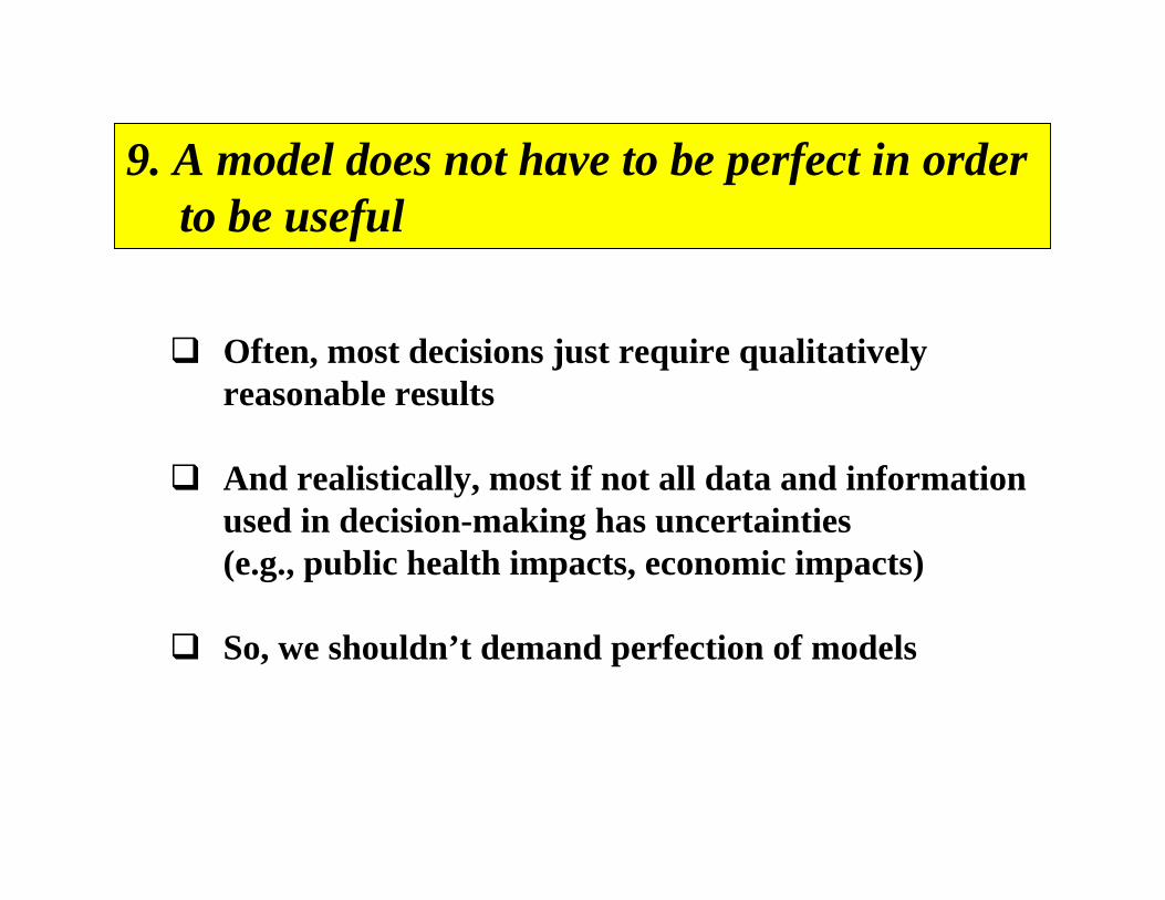
9. A model does not have to be perfect in order to be useful
Often, most decisions just require qualitatively reasonable results
And realistically, most if not all data and information used in decision-making has uncertainties (e.g., public health impacts, economic impacts)
So, we shouldn’t demand perfection of models
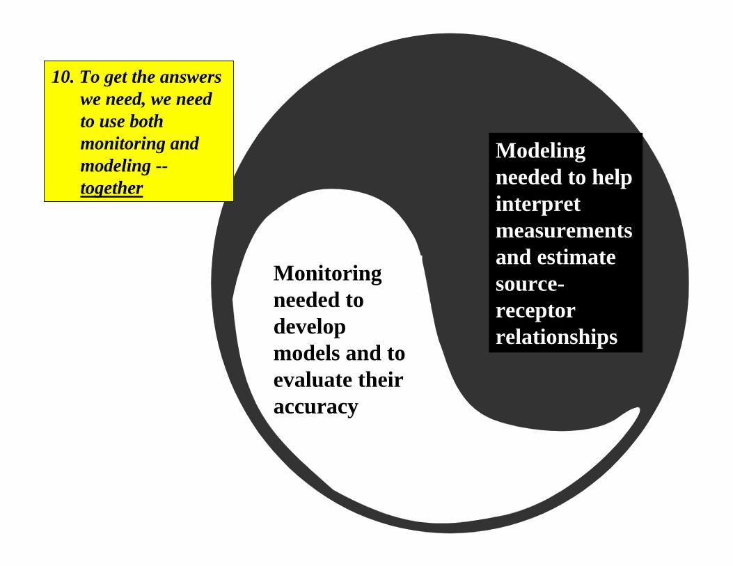
Modeling needed to help interpret measurements and estimate source-receptor relationships
Monitoring needed to develop models and to evaluate their accuracy
10. To get the answers we need, we need to use both monitoring and modeling --together
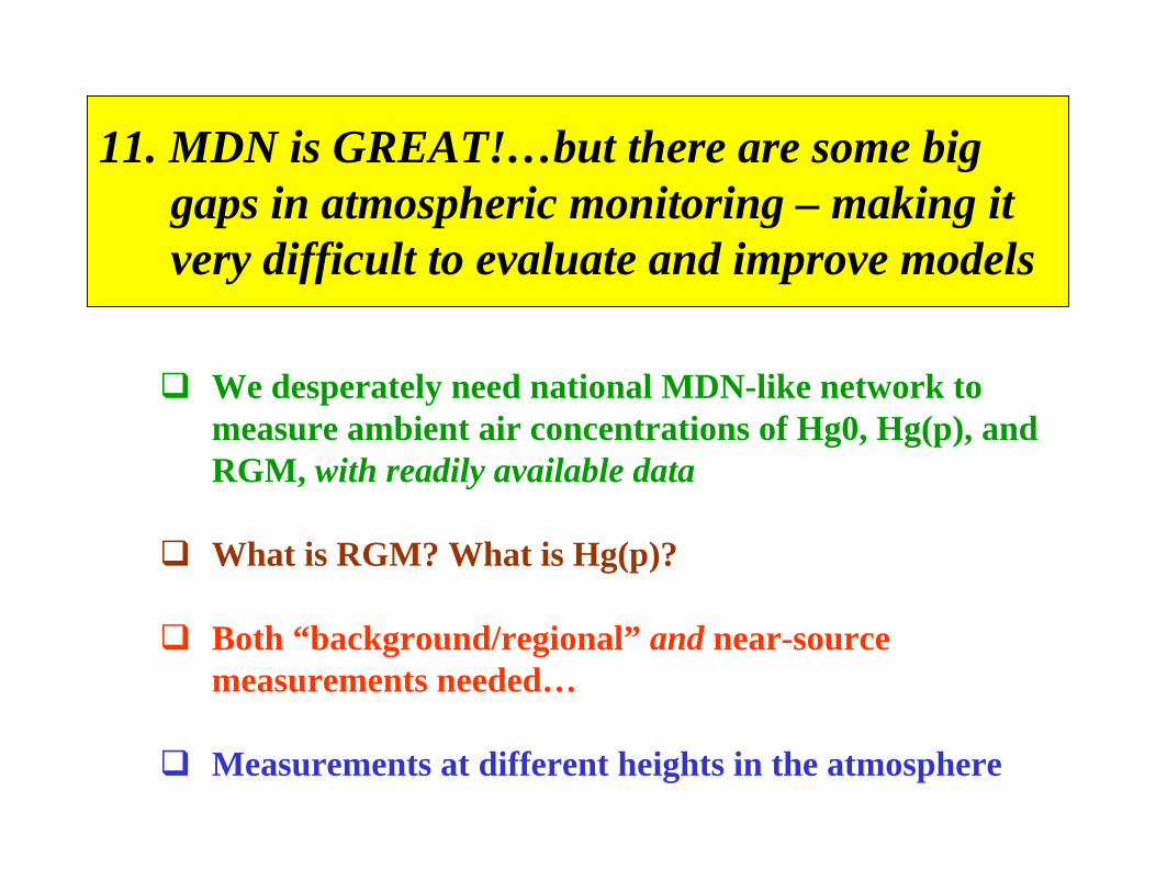
11. MDN is GREAT!…but there are some big gaps in atmospheric monitoring – making it very difficult to evaluate and improve models
We desperately need national MDN-like network to measure ambient air concentrations of Hg0, Hg(p), and RGM, with readily available data
What is RGM? What is Hg(p)?
Both “background/regional” and near-source measurements needed…
Measurements at different heights in the atmosphere
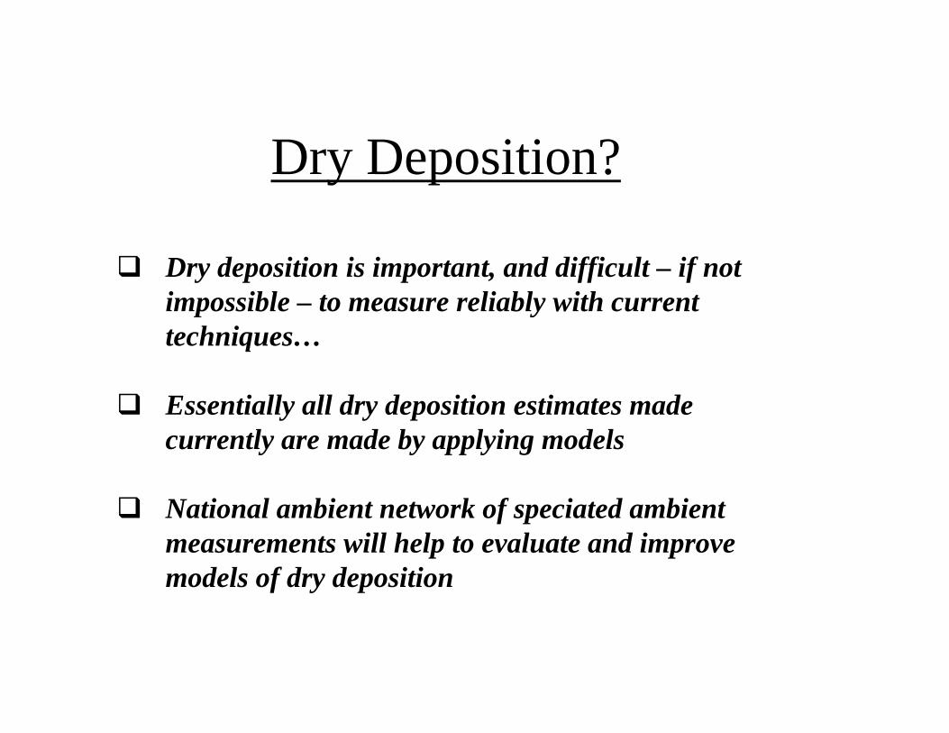
Dry deposition is important, and difficult – if not impossible – to measure reliably with current techniques…
Essentially all dry deposition estimates made currently are made by applying models
National ambient network of speciated ambient measurements will help to evaluate and improve models of dry deposition
Dry Deposition?
Source-Apportionmentwhere does the mercury in
mercury deposition come from?
Source-apportionment answers depend on
where you are, and
when you are
(and the effects of depositionwill be different in each ecosystem)
For areas without large emissions sources
the deposition may be relatively low,but what deposition there is may largely come from natural and global sources
For areas with large emissions sources
the deposition will be higherand be more strongly influenced by these large emissions sources...
Lake
Erie
Lake
Mic
higa
n
Lake
Sup
erio
r
Lake
Hur
on
Lake
Ont
ario
Lk C
ham
plai
n
Lake
Tah
oe
Puge
t Sou
nd
Mes
a Ve
rde
NP
Mob
ile B
ay
Mam
mot
h C
ave
NP
Sand
y H
ook
Long
Isla
nd S
ound
Adi
rond
ack
Park
Mas
s B
ay
Aca
dia
NP
Gul
f of M
aine
Che
sape
ake
Bay
Che
s B
ay W
S
0
5
10
15
(ug/
m2-
year
)H
g D
epos
ition
Flu
x (1
999
base
)
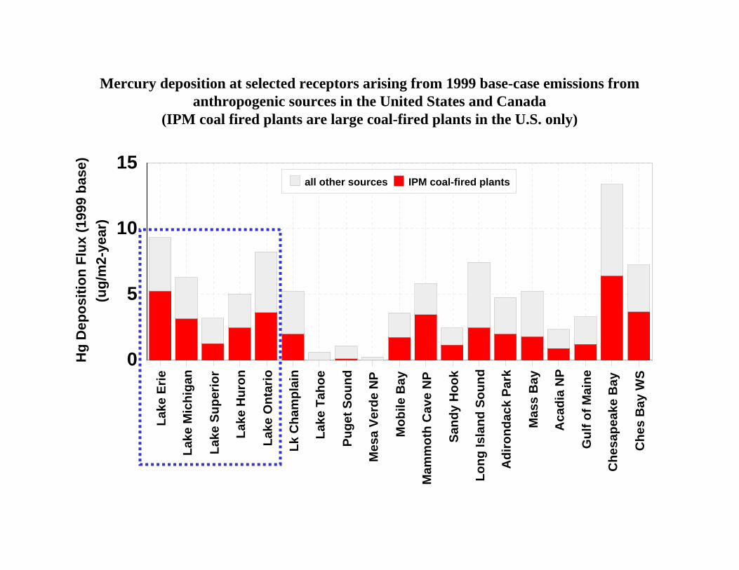
all other sources IPM coal-fired plants
Mercury deposition at selected receptors arising from 1999 base-case emissions from anthropogenic sources in the United States and Canada
(IPM coal fired plants are large coal-fired plants in the U.S. only)
Example of modeling results:Chesapeake Bay
Cohen, M., Artz, R., Draxler, R., Miller, P., Poissant, L., Niemi, D., Ratte, D., Deslauriers, M., Duval, R., Laurin, R., Slotnick, J., Nettesheim, T., McDonald, J.“Modeling the Atmospheric Transport and Deposition of Mercury to the Great Lakes.” Environmental Research 95(3), 247-265, 2004.
Note: Volume 95(3) is a Special Issue: "An Ecosystem Approach to Health Effects of Mercury in the St. Lawrence Great Lakes", edited by David O. Carpenter.
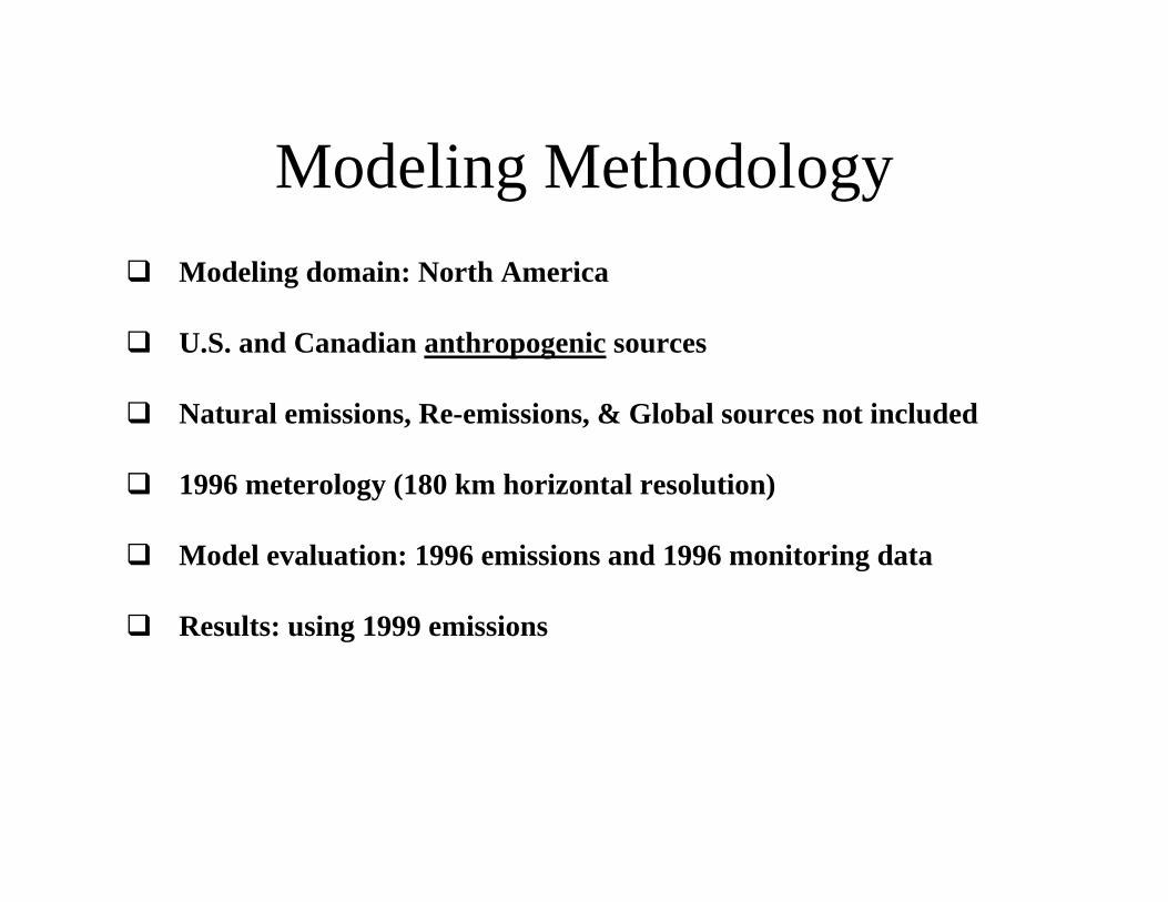
Modeling domain: North America
U.S. and Canadian anthropogenic sources
Natural emissions, Re-emissions, & Global sources not included
1996 meterology (180 km horizontal resolution)
Model evaluation: 1996 emissions and 1996 monitoring data
Results: using 1999 emissions
Modeling Methodology
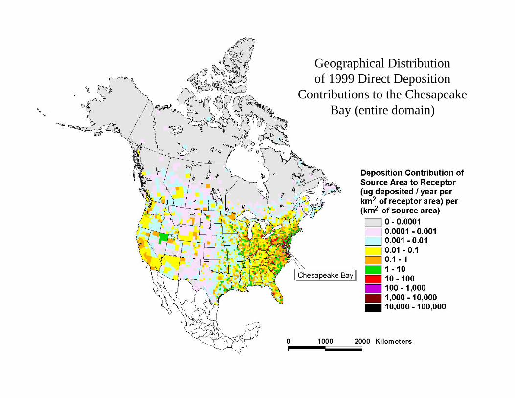
Geographical Distributionof 1999 Direct Deposition
Contributions to the Chesapeake Bay (entire domain)
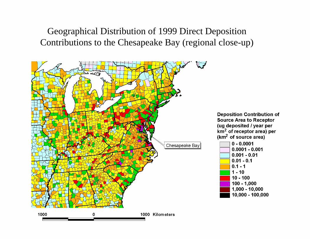
Geographical Distribution of 1999 Direct Deposition Contributions to the Chesapeake Bay (regional close-up)
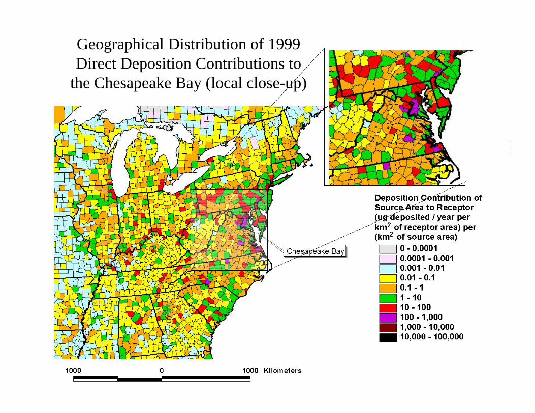
Geographical Distribution of 1999 Direct Deposition Contributions to
the Chesapeake Bay (local close-up)
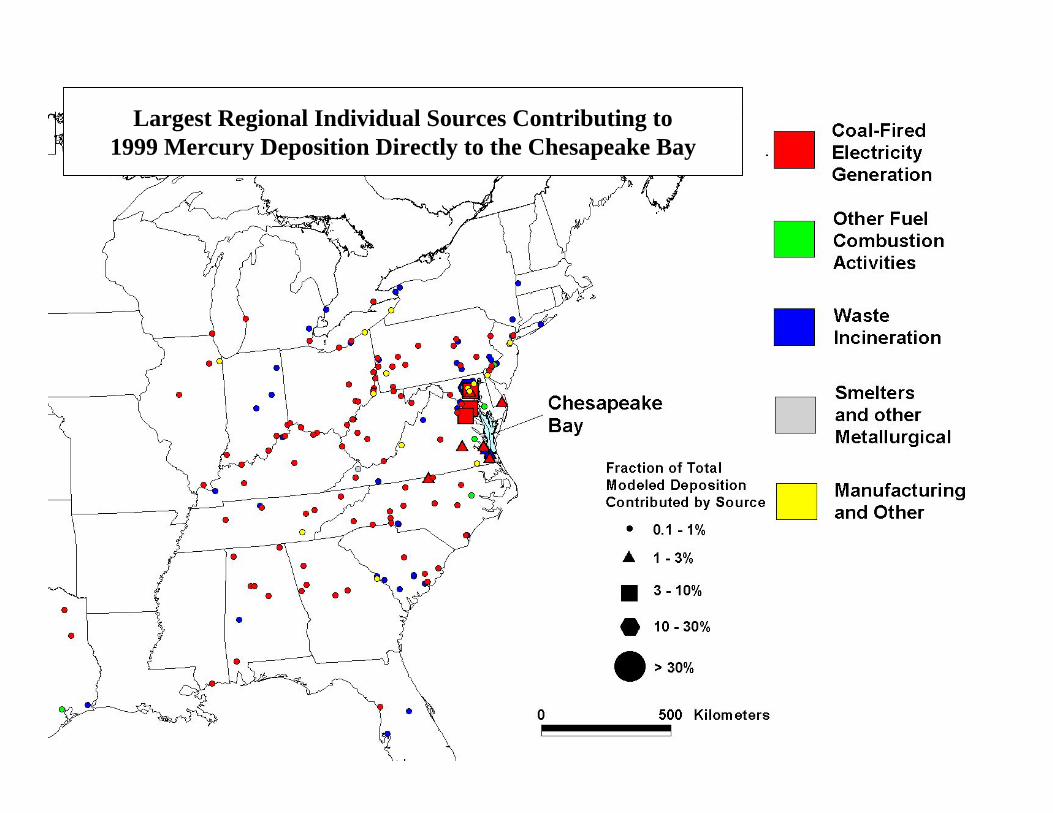
Largest Regional Individual Sources Contributing to1999 Mercury Deposition Directly to the Chesapeake Bay
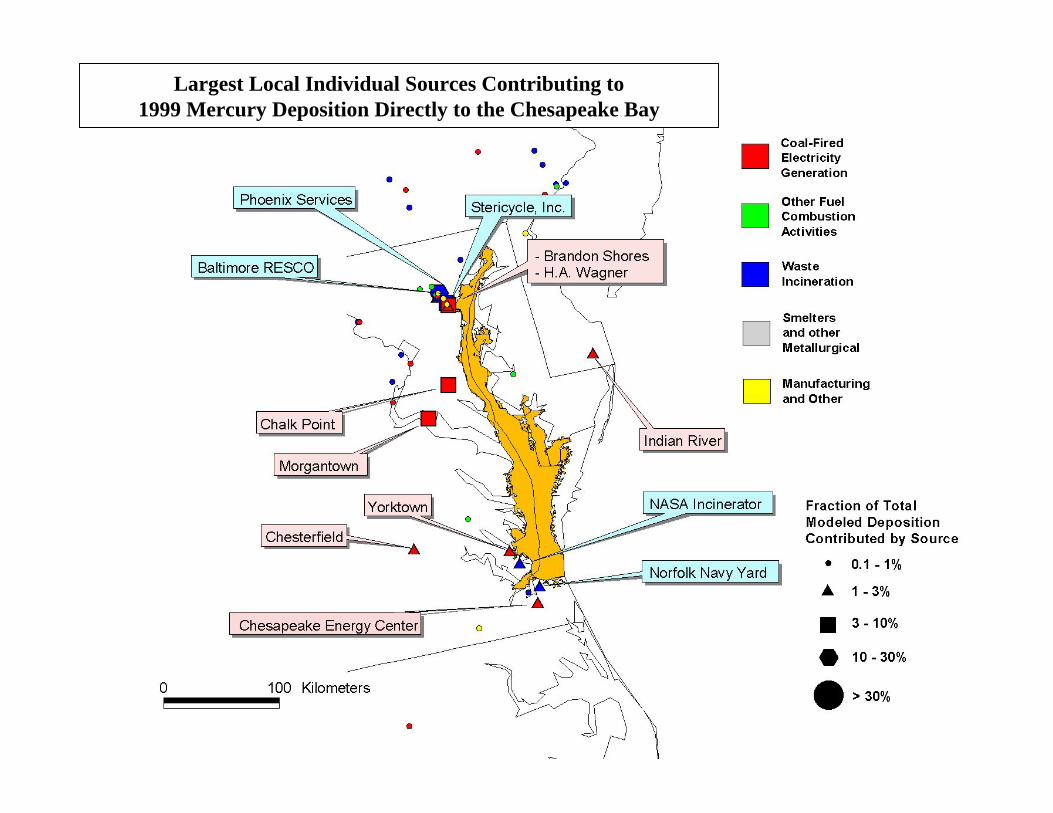
Largest Local Individual Sources Contributing to1999 Mercury Deposition Directly to the Chesapeake Bay
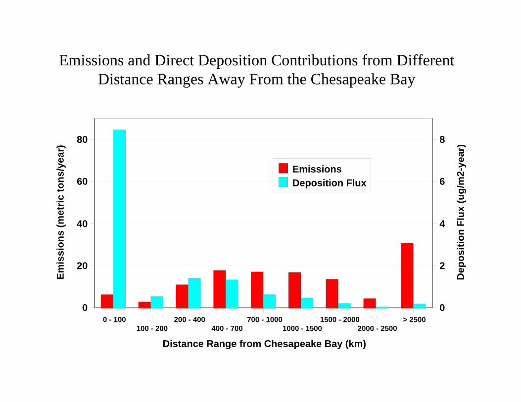
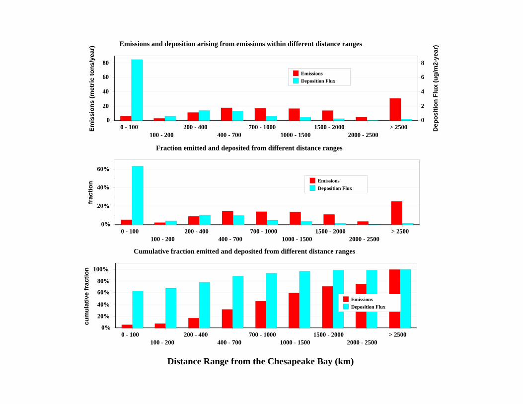
Emissions and Direct Deposition Contributions from Different Distance Ranges Away From the Chesapeake Bay
0 - 100100 - 200
200 - 400400 - 700
700 - 10001000 - 1500
1500 - 20002000 - 2500
> 2500
Distance Range from Chesapeake Bay (km)
0
20
40
60
80
Emis
sion
s (m
etric
tons
/yea
r)
0
2
4
6
8
Dep
ositi
on F
lux
(ug/
m2-
year
)
EmissionsDeposition Flux
Distance Range from the Chesapeake Bay (km)
0 - 100100 - 200
200 - 400400 - 700
700 - 10001000 - 1500
1500 - 20002000 - 2500
> 25000
20
40
60
80
Emis
sion
s (m
etric
tons
/yea
r)
0
2
4
6
8
Dep
ositi
on F
lux
(ug/
m2-
year
)
EmissionsDeposition Flux
Emissions and deposition arising from emissions within different distance ranges
0 - 100100 - 200
200 - 400400 - 700
700 - 10001000 - 1500
1500 - 20002000 - 2500
> 25000%
20%
40%
60%
frac
tion Emissions
Deposition Flux
Fraction emitted and deposited from different distance ranges
0 - 100100 - 200
200 - 400400 - 700
700 - 10001000 - 1500
1500 - 20002000 - 2500
> 25000%
20%
40%
60%
80%
100%
cum
ulat
ive
frac
tion
EmissionsDeposition Flux
Cumulative fraction emitted and deposited from different distance ranges
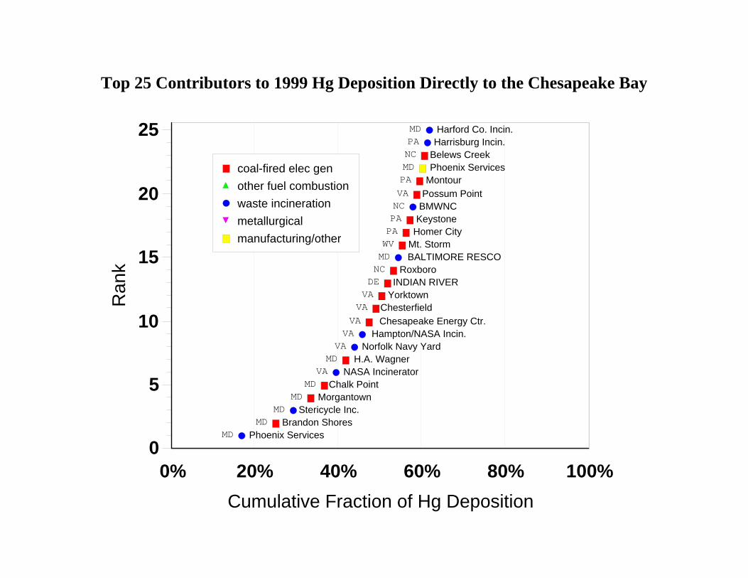
Top 25 Contributors to 1999 Hg Deposition Directly to the Chesapeake Bay
Phoenix ServicesBrandon Shores
Stericycle Inc. Morgantown
Chalk PointNASA Incinerator
H.A. WagnerNorfolk Navy Yard
Hampton/NASA Incin.Chesapeake Energy Ctr.Chesterfield Yorktown
INDIAN RIVER Roxboro
BALTIMORE RESCO Mt. Storm Homer City Keystone BMWNC
Possum Point Montour
Phoenix ServicesBelews CreekHarrisburg Incin.Harford Co. Incin.
MD MD
MD MD
MD VA MD VA VA VA VA VA DE NC MD WV PA PA NC VA PA MD NC PA MD
0% 20% 40% 60% 80% 100%Cumulative Fraction of Hg Deposition
0
5
10
15
20
25R
ank
coal-fired elec genother fuel combustionwaste incinerationmetallurgicalmanufacturing/other
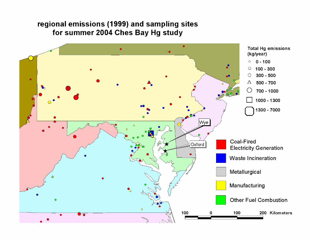
Summer 2004 Chesapeake Bay Atmospheric Hg Study(June – August 2004)
• NOAA Cooperative Oxford Lab: Bob Wood
• NOAA Air Resources Lab Atmospheric Turbulence and Diffusion Division (ATDD): Steve Brooks
• NOAA Air Resources Lab HQ Division: Winston Luke, Paul Kelley, Mark Cohen, Richard Artz
• NOAA Chesapeake Bay Office: Maggie Kerchner
• Frontier GeoSciences: Bob Brunette, Gerard van der Jagt, Eric Prestbo
• Univ. of MD Wye Res. and Educ. Center: Mike Newall
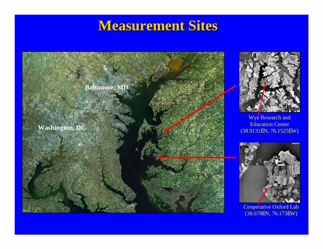
Cooperative Oxford Lab(38.678EN, 76.173EW)
Wye Research andEducation Center
(38.9131EN, 76.1525EW)
Baltimore, MD
Washington, DC
Measurement SitesMeasurement Sites
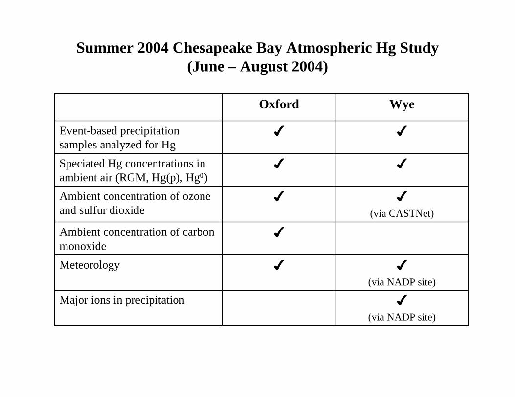
Ambient concentration of carbon monoxide
(via NADP site)Major ions in precipitation
(via NADP site)Meteorology
(via CASTNet)Ambient concentration of ozone and sulfur dioxide
Speciated Hg concentrations in ambient air (RGM, Hg(p), Hg0)
Event-based precipitation samples analyzed for Hg
WyeOxford
Summer 2004 Chesapeake Bay Atmospheric Hg Study(June – August 2004)
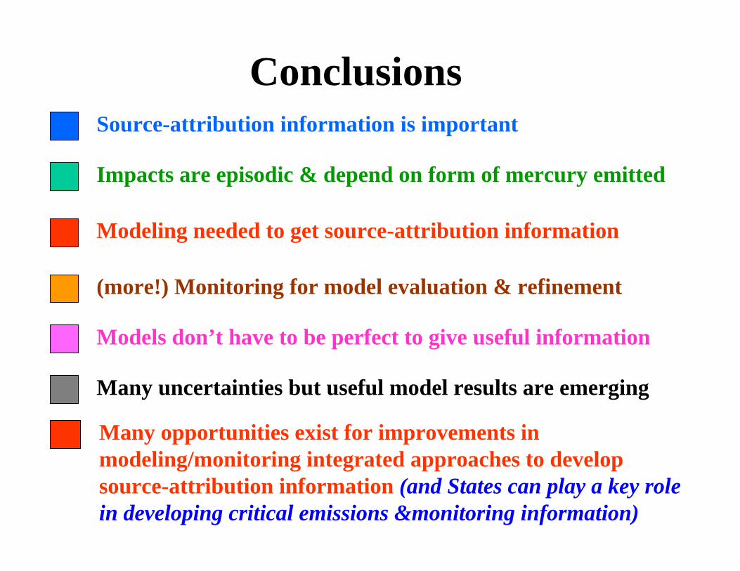
Conclusions
Impacts are episodic & depend on form of mercury emitted
Source-attribution information is important
Modeling needed to get source-attribution information
(more!) Monitoring for model evaluation & refinement
Many uncertainties but useful model results are emerging
Models don’t have to be perfect to give useful information
Many opportunities exist for improvements in modeling/monitoring integrated approaches to develop source-attribution information (and States can play a key role in developing critical emissions &monitoring information)
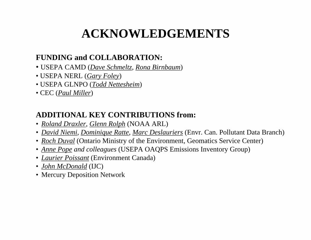
FUNDING and COLLABORATION:• USEPA CAMD (Dave Schmeltz, Rona Birnbaum)• USEPA NERL (Gary Foley)• USEPA GLNPO (Todd Nettesheim)• CEC (Paul Miller)
ACKNOWLEDGEMENTS
ADDITIONAL KEY CONTRIBUTIONS from:• Roland Draxler, Glenn Rolph (NOAA ARL)• David Niemi, Dominique Ratte, Marc Deslauriers (Envr. Can. Pollutant Data Branch)• Roch Duval (Ontario Ministry of the Environment, Geomatics Service Center)• Anne Pope and colleagues (USEPA OAQPS Emissions Inventory Group)• Laurier Poissant (Environment Canada)• John McDonald (IJC)• Mercury Deposition Network