arX

iv:a

stro

-ph/

0703

163v

1 7

Mar

200

7submitted to ApJ March 2, 2007Preprint typeset using LATEX style emulateapj v. 10/09/06

ORIGINS OF ECCENTRIC EXTRASOLAR PLANETS: TESTING THE PLANET–PLANET SCATTERINGMODEL

Eric B. Ford1,2 and Frederic A. Rasio3

submitted to ApJ March 2, 2007

ABSTRACT

Any planetary system with two or more giant planets may become dynamically unstable, leading tocollisions or ejections through strong planet–planet scattering. Following an ejection, the other planetis left in a highly eccentric orbit. Previous studies for simple initial configurations with two equal-mass planets revealed two discrepancies between the results of numerical simulations and the observedorbital elements of extrasolar planets: the potential for frequent collisions between giant planets anda narrow distribution of final eccentricities following ejections. Here, we show that simulations fortwo planets with unequal masses predict a reduced frequency of collisions and a broader range offinal eccentricities. We show that the two-planet scattering model can easily reproduce the observedeccentricities with a plausible distribution of planet mass ratios. Further, the two-planet scatteringmodel predicts a maximum eccentricity of about 0.8, independent of the distribution of planet massratios. This compares favorably with current observations and will be tested by future planet discov-eries. Moreover, we show that the combination of planet–planet scattering and tidal circularizationmay be able to explain the existence of some giant planets with very short period orbits. However, thepresence of giant planets in circular orbits at slightly larger orbital periods (small enough to requiresignificant migration, but large enough that tidal circularization is ineffective) is more difficult toexplain. As part of this work, we also re-examine and discuss various possible correlations betweeneccentricities and other properties of observed extrasolar planets. We demonstrate that the observeddistribution of planet masses, orbital periods, and eccentricities can provide constraints for models ofplanet formation and evolution.

Subject headings: planetary systems — planetary systems: formation — planets and satellites: general— celestial mechanics

1. INTRODUCTION

For several centuries, theories of planet formation hadbeen designed to explain our own Solar System, but thefirst few discoveries of extrasolar planets immediatelysent theorists back to the drawing board. These discov-eries led to the realization that planet formation theorymust be generalized to explain a much wider range ofproperties for planetary systems. For example, it hadlong been assumed that planets formed in circular or-bits because of strong eccentricity damping in the proto-planetary disk and that their orbits would later remainnearly circular (i.e., with eccentricity e ≤0.1; Lissauer1993, 1995). However, over half of the extrasolar planetsbeyond 0.1 AU have eccentricities e ≥0.3, and two haveeccentricities larger than 0.9.

The planets in eccentric orbits are generally believed tohave formed on nearly circular orbits but later evolvedto their presently observed large eccentricities. Theo-rists have suggested numerous mechanisms to excite theorbital eccentricity of giant planets. These include:

a) secular perturbations due to a distant stellar ormassive planetary companion (Holman, Touma, &Tremaine 1997; Mazeh et al. 1997; Ford, Kozinsky,& Rasio 2000; Takeda & Rasio 2005),

Electronic address: eford@cfa.harvard.edu1 Hubble Fellow2 Harvard-Smithsonian Center for Astrophysics, Mail Stop 51,

60 Garden Street, Cambridge, MA 021383 Department of Physics and Astronomy, Northwestern Univer-

sity, Evanston, IL 60208

b) perturbations from passing stars (Laughlin &Adams 1998; Hurley & Shara 2002; Zakamska &Tremaine 2004),

c) strong planet–planet scattering events in plane-tary systems with either a few planets (Rasio &Ford 1996; Weidenschilling & Marzari 1996; Ford,Havlickova, & Rasio 2001 (FHR); Marzari & Wei-denschilling 2002; Yu & Tremaine 2001; Ford, Ra-sio & Yu 2003; Veras & Armitage 2004, 2005,2006) or many planets (Lin & Ida 1997; Levisonet al. 1998; Papaloizou & Terquem 2001; Adams &Laughlin 2003l Goldreich, Lithwick, & Sari 2004;Ford & Chiang 2007; Juric & Tremaine 2007),

d) interactions of orbital migration with mean-motionresonances (Chiang & Murray 2002; Kley 2000;Kley et al. 2004, 2005; Lee & Peale 2002; Tsiga-nis et al. 2005),

e) resonances between secular perturbations and pre-cession induced by general relativity, stellar oblate-ness, and/or a remnant disk (Ford et al. 2000; Na-gasawa et al. 2003; Adams & Laughlin 2006),

f) interactions with a planetesimal disk (Murrary etal. 1998),

g) interactions with a gaseous proto-planetary disk(Goldreich & Tremaine 1980; Artymowicz 1992;Papaloizou et al. 2001; Goldreich & Sari 2003;Ogilvie & Lubow 2003),

2 Ford and Rasio

h) asymmetric stellar jets (Namouni 2005, 2006), and

i) hybrid scenarios that combine aspects of more thanone of the above mechanisms (e.g., Marzari et al.2005; Sandor & Kley 2006; Malmberg et al. 2006).

Some of mechanisms (a, b) inevitably influence the evo-lution of some planetary systems, but are not able toexplain the ubiquity of eccentric giant planets (Zakam-ska & Tremaine 2004; Takeda & Rasio 2005). Obser-vations of multiple planet systems have provided strongevidence that other mechanisms (c, d) are also signifi-cant in altering planet’s orbital eccentricities. For ex-ample, the dramatic eccentricity oscillations of υ And cprovide an upper limit on the timescale for eccentricityexcitation in υ And (≃ 100yr) and strong evidence forplanet–planet scattering in this system (Ford, Lystad &Rasio 2005). Other multiple planet systems may alsoexhibit similar behavior (Barnes & Greenberg 2006ab).As another example, the detection of pairs of planets in2:1 mean motion resonances (e.g., GJ 876 b & c) sug-gests that smooth convergent migration likely occurredin these systems. Additionally, the fact that migrationmodels can simultaneously match the observed eccentric-ities for both planets b & c suggests eccentricity excita-tion was related to the migration and resonant capture inthis system (Lee & Peale 2002; Kley et al. 2005). It is notclear if the remaining mechanisms (e-h) are important forshaping the actual distribution of planet eccentricities.

In this paper, we expand upon the original planet–planet scattering model of Rasio & Ford (1996) and FHR.First, we evaluate some potential origins of dynamicalinstabilities that result in close encounters and strongplanet–planet scattering in §2. In §3, we present theresults of n-body simulations of planet–planet scatteringfor systems with two giant planets of unequal masses.Then, in §4, we compare the predictions of eccentricityexcitation models with the eccentricities of the knownextrasolar planets. In §5, we discuss the implicationsof our work for theories of eccentricity excitation anddamping and suggest how future observations can furthertest theories for eccentricity excitation.

2. ORIGIN OF INSTABILITY

While some authors have simulated multiple planetsystems beginning with the planet formation stage, com-putational cost has limited such simulations to a smallportion of the disk and/or small number of initial condi-tions (e.g., Kokubo & Ida 1998; Levison, Lissauer, &Duncan 1998). Since dynamically unstable planetarysystems are highly chaotic, we can only investigate thestatistical properties of an ensemble of systems with sim-ilar initial conditions. Thus, most investigations of dy-namical instabilities in multiple planet systems proceedby simulating systems after planets have formed and per-turbations due to the protoplanetary disk are no longersignificant. The planets are placed on plausible initialorbits and numerically integrated according to the grav-itational potential of the central star and other planets.

Clearly, the choice of initial conditions will determinewhether the systems are dynamically stable and will af-fect the outcome of unstable systems. Our simulationsof planet–planet scattering typically begin with closelyspaced giant planets (e.g., Rasio & Ford 1996; FHR).This is necessary for dynamical instabilities to occur in

systems with only two planets initially on circular orbits.For two-planet systems, there is a sharp transition fromrigorous Hill stability to chaos and strong interactions.Therefore, one potential concern about the relevance ofdynamical instabilities is whether the necessary initialconditions will manifest themselves in the two-planetconfigurations that occur in nature. In this section, wedescribe several possible mechanisms that could lead todynamical instabilities in two-planet systems, includingmass growth through accretion, dissipation of the proto-planetary disk, and orbital migration. Additionally, thesecular evolution of systems with more than two planetsprovides a naturally mechanism for triggering dynamicalinstabilities, even long after the protoplanetary disk hasdissipated and planets are fully assembled (Chatterjee etal. 2007).

According to the standard core accretion model, oncea rocky planetary core reaches a critical mass, it rapidlyaccretes the gas within its radius of influence in a cir-cumstellar disk. Thus, the semi-major axis of a plan-etary core is determined by the collisional evolution ofprotoplanets, while the mass of a giant planet is deter-mined by the state of the gaseous disk when the corereaches the critical mass (Lissauer 1993). Two planetarycores could form with an initial separation sufficient toprevent close encounters while their masses are less thanthe critical mass for runaway accretion, but insufficientto prevent a dynamical instability after the onset of rapidmass growth due to gas accretion (Pollack et al. 1996).

The accumulation of random velocities provides an-other possible source of a dynamical instability. Assum-ing planets form in the presence of a dissipative disk,they are expected to form on nearly circular and copla-nar orbits. While the timescale for dissipation in the diskremains shorter than the timescales for eccentricity ex-citation, eccentricities and inclinations will be damped,preventing close encounters. As the disk dissipates, ec-centricity damping becomes less significant, so mutualplanetary perturbations can excite significant eccentrici-ties and inclinations and lead to close encounters betweenplanets.

Finally, the discovery of giant planets at small orbitalseparations suggests that large-scale orbital migrationmay be common. In multiple planet systems, conver-gent migration (i.e., with the ratio of semi-major axesapproaching unity) could increase the strength of mu-tual planetary perturbations, excite eccentricities (eitherbefore or after resonant capture), and result in planetscattering (Sandor & Kley 2005).

In contrast to the case of two-planet systems, thereis no sharp stability criterion for three-planet systems.Three-planet systems can be unstable even for initial or-bital spacings significantly greater than would be nec-essary for similar two-planet systems to be unstable(Chambers, Wetherill & Boss 1996). Additionally, suchsystems can evolve quasi-stably for very long times,∼ 106 − 1010 yr, before chaos finally leads to close en-counters and strong planet–planet scattering (Marzari& Weidenschilling 2002; Chatterjee at al. 2007). Thislonger timescale until close encounters could allow suffi-cient time for three or more planets to form via eitherthe disk instability or core accretion models.

If protoplanetary disks form many planets nearly si-multaneously, then planet–planet scattering may lead to

Eccentric Extrasolar Planets 3

a phase of dynamical relaxation. Several researchers havenumerically investigated the dynamics of planetary sys-tems with ∼ 10 − 100 planets (Lin & Ida 1997; Levisonet al. 1998; Papaloizou & Terquem 2001, 2002; Adams &Laughlin 2003; Barnes & Quinn 2004; Juric & Tremaine2007). Initially, such systems are highly chaotic and closeencounters are common. The close encounters lead toplanets colliding (creating a more massive planet) and/orplanets being ejected from the system, depending on theorbital periods and planet radii. Either process results inthe number of planets in the system being reduced andthe typical separations between planets increasing. Thesystem gradually evolves from a highly unstable state toquieter states, which can last longer before the next colli-sion or ejection. Such systems typically evolve ultimatelyto a final state with 1–3 eccentric giant planets that willpersist for the lifetime of the star (Laughlin & Adams2003; Juric & Tremaine 2007).

With so many possibilities for triggering dynamical in-stabilities in multiple planet systems, we expect thatthese processes may be rather ubiquitous. While realplanetary systems likely have more than two massivebodies, simulations of relatively simple systems (e.g.,with just two giant planets) facilitate the systematicstudy of the relevant physics and help develop intuitionfor thinking about the evolution of more complex sys-tems.

3. NUMERICAL INVESTIGATION OF PLANET–PLANETSCATTERING

In the previous section, we argued that if planet forma-tion commonly results in planetary systems with multipleplanets, then it should be expected that the initial con-figurations will not be dynamically stable for time spansorders of magnitude longer than the timescale for planetformation. Shortly after the discovery of the first eccen-tric extrasolar planets, Rasio & Ford (1996) conductedMonte Carlo integrations of planetary systems contain-ing two equal-mass planets initially placed just inside theHill stability limit (Gladman 1993). They numericallyintegrated the orbits of such systems until there was acollision, or one planet was ejected from the system, orsome maximum integration time was reached. The twomost common outcomes were collisions between the twoplanets, producing a more massive planet in a nearly cir-cular orbit between the two initial orbits, and ejectionsof one planet from the system while the other planet re-mains in a tighter orbit with a large eccentricity. Therelative frequency of these two outcomes depends on theratio of the planet radius to the initial semi-major axis.

While this model could naturally explain how planetsacquire large eccentricities, FHR performed a large en-semble of planet–planet scattering experiments to com-pare the resulting planetary systems to the observed sam-ple and found two important differences. First, for therelevant radii and semi-major axes, collisions were morefrequent in the simulations than nearly circular orbitsamong the known extrasolar planets.

However, the branching ratios from those simulationsmay not be appropriate for realistic planetary systems.Since there is a sharp and rigorous Hill stability limit fortwo-planet systems, the initial conditions placed the twoplanets in orbits with a relatively small separation. SinceFHR also assigned the planets small initial eccentricities

and inclinations, the planets initially had a small rela-tive velocity at conjunction (compared to their circularvelocity) and gravitational focusing increased the rate ofcollisions early on in the simulations. The rate of col-lisions drops significantly (for the systems that survivelong enough) once the planets have had time to exciteeach other’s eccentricities. Thus, the fraction of systemsthat result in collisions is likely sensitive to the initialconditions.

To determine the fraction of actual two-planet systemsthat result in collisions more accurately, future studieswould need to model the onset of the instability more re-alistically. Unfortunately, direct n-body integrations ofyoung planetary systems with small bodies are extremelycomputationally demanding. The significance of initialconditions is less pronounced for n-body integrations ofsystems with three or more planets, since more distantinitial spacings can be used, so that all close encoun-ters occur only after the planets have excited each otherseccentricities. Despite these potential complications, itcan be useful to study relatively simple model systems todevelop intuition for more complex problems and to un-derstand the limitations of simple models. In that spirit,FHR reported the results of planet–planet scattering ex-periments involving two equal-mass planets, while herewe report the results of planet–planet scattering experi-ments involving two planets of unequal masses.

The more significant shortcoming of the two equal-mass planet scattering model identified by FHR was that,in systems leading to one ejection, the eccentricity dis-tribution of the remaining planet was concentrated in anarrow range and greater than the typical eccentricity ofthe known extrasolar planets (See Fig. 2, right, rightmostcurve). FHR speculated that planet–planet scatteringinvolving two planets of unequal masses would result inplanets remaining with a broader distribution of eccen-tricities. In this section, we present results that confirmthis speculation and quantify the resulting eccentricities.

3.1. Initial Conditions

We used the mixed variable symplectic algorithm ofWisdom & Holman (1991), modified to allow for closeencounters between planets as implemented in the pub-licly available code Mercury (Chambers 1999). The re-sults presented below are based on ∼ 104 numerical in-tegrations. Our numerical integrations were performedfor a system containing two planets, with mass ratios10−4 < µi < 10−2, where µi ≡ mi/M⋆, mi is themass of the ith planet, and M⋆ is the mass of the cen-tral star. A mass ratio of µi ≃ 10−3 corresponds tom ≃ 1 MJup for M = 1 M⊙, where MJup is the massof Jupiter and M⊙ is the mass of the sun. The initialsemimajor axis of the inner planet (a1,init) was set tounity and the initial semimajor axis of the outer planet(a2,init) was drawn from a uniform distribution rangingfrom 0.9 ·a1,init (1 + ∆c) to a1,init (1 + ∆c), where 1+∆c

is the critical semi-major axis ratio above which Hill sta-bility is guaranteed for initially circular coplanar orbits,

and ∆c ≃ 2.4 × (µ1 + µ2)1/3

(Gladman 1993). The ini-tial eccentricities were distributed uniformly in the rangefrom 0 to 0.05, and the initial relative inclination in therange from 0◦ to 2◦. All remaining angles (longitudesand phases) were randomly chosen between 0 and 2π.Throughout this paper we quote numerical results in

4 Ford and Rasio

units such that G = a1,init = M⋆ = 1, where G is thegravitational constant. In these units, the initial orbitalperiod of the inner planet is P1 ≃ 2π.

Throughout the integrations, close encounters betweenany two bodies were logged, allowing us to use a singleset of n-body integrations to study the outcome of sys-tems with a a wide range of planetary radii. We considera range of radii to allows for the uncertainty in both thephysical radius and the effective collision radius allowingfor dissipation in the planets. When two planets col-lided, mass and momentum conservation were assumedto compute the final orbit of the resulting single planet.

Each run was terminated when one of the followingfour conditions was encountered: (i) one of the two plan-ets became unbound (which we defined as having a radialdistance from the star of 2000 a1,init); (ii) a collision be-tween the two planets occurred assuming Ri/a1,init =Rmin/a1,init = 1 RJup/5 AU = 0.95 × 10−4, where RJup

is the radius of Jupiter; (iii) a close encounter occurredbetween a planet and the star (defined by having aplanet come within rmin/a1,init = 10 R⊙/5 AU = 0.01of the star); (iv) the integration time reached tmax =5 · 106 − 2 · 107 depending on the masses of the plan-ets. These four types will be referred to as “collisions,”meaning a collision between the two planets, “ejections,”meaning that one planet was ejected to infinity, “stargrazers,” meaning that one planet had a close pericenterpassage, and “two planets.”

3.2. Results

We began by conducting an exploratory set of inte-grations using a wide variety of planet masses (10−3 ≤mi/M < 10−2). The probabilities for the four out-comes (collisions, ejections, star grazers, and two plan-ets) depend on the mass of both planets, the final or-bital properties of the system within one of these out-comes depended on the ratio of planet masses, but notthe total planet mass. Therefore, we focused our n-body integrations of a series of seven sets of integra-tions with a constant total planet mass ratio, but varyingβ ≡ m1/(m1 + m2). We chose a somewhat large totalplanet mass ratio, (m1 + m2)/M⋆ = 6 × 10−3, so as toaccelerate the evolution of the planetary systems and re-duce the computational cost of the simulations.

3.2.1. Collisions

Collisions leave a single, larger planet in orbit aroundthe star. Near the time of a collision, the energy in thecenter-of-mass frame of the two planets is much smallerthan the gravitational binding energy of a giant planetto the star. Therefore, we model the collisions as com-pletely inelastic and assume that the two giant planetssimply merge together while conserving total momentumand mass. Using this assumption, the final orbit has asemi-major axis between the two initial semi-major axes,a small eccentricity, and a small inclination. In fact, wefind that the final semi-major axis is only slightly lessthan would be estimated on the basis of energy conser-vation,

af

a1≃

[

m1

m1 + m2+

m2a1

(m1 + m2) a2

]−1

, (1)

where af is the final semi-major axis of the remainingplanet. This compares favorably with the results of our

simulations and the magnitude of the deviations can beapproximated (see appendix of FHR). We find that thefractions of our integrations that result in collisions de-creases for more more extreme planet mass ratios (assum-ing constant total planet mass). While collisions betweenplanets may affect the masses of extrasolar planets, a sin-gle collision between two massive planets does not causesignificant orbital migration or eccentricity growth if theplanets are initially on low-eccentricity, low-inclinationorbits near the Hill stability limit. Therefore, we shiftour attention to those simulations that resulted in ejec-tions.

3.2.2. Ejections

Since the escaping planet typically leaves the systemwith a very small (positive) energy, energy conservationsets the final semimajor axis of the remaining planetslightly less than

af

a1≃

[

m1

mf+

a1m2

a2mf

]−1

(2)

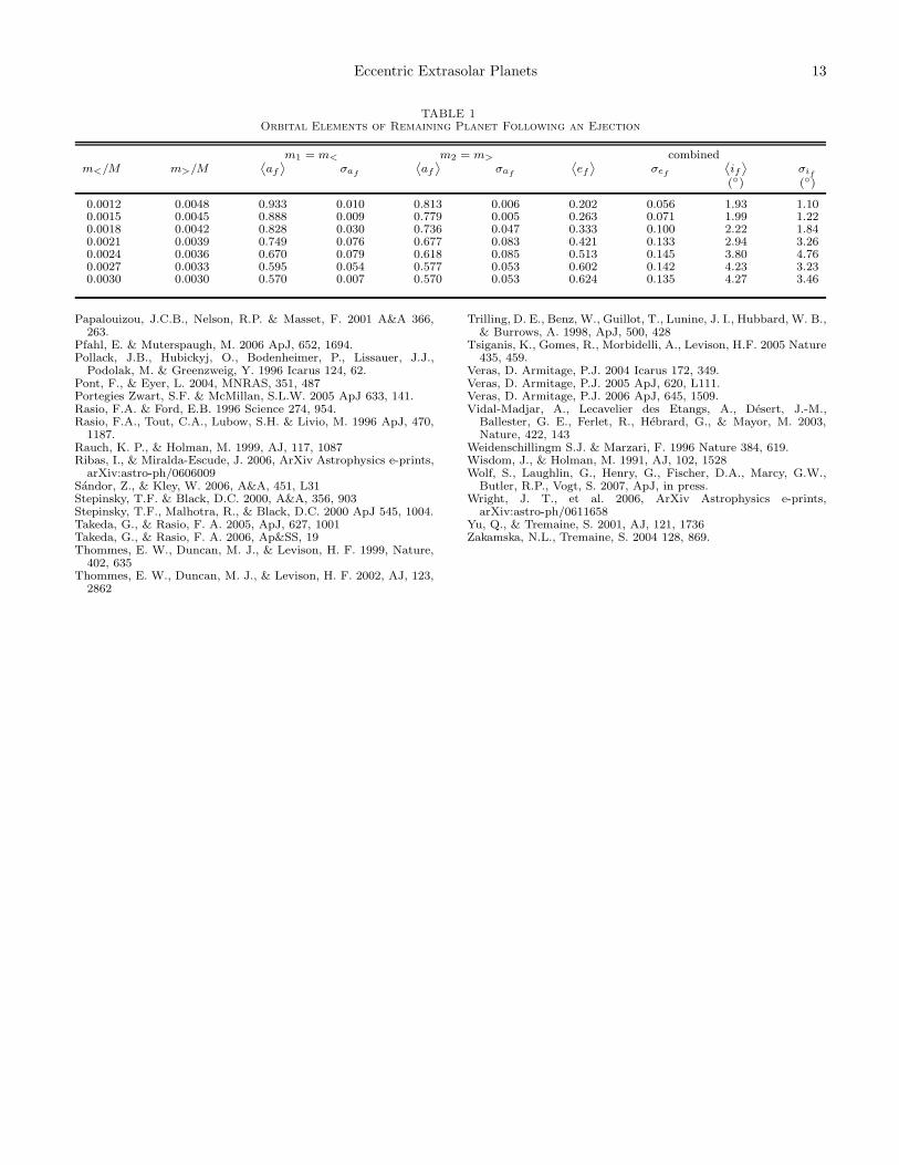
Thus, the final semi-major axis of the planet left be-hind after an ejection depends on whether the more mas-sive planet initially had the smaller or larger semi-majoraxis. Otherwise, the order of the planets makes littledifference. Even in simulations with equal mass planets(β = 0.5), we that the outer planet typically accounts for≃ 55% of the ejections. When β is reduced only slightlyto 0.45 or 0.40, then ≃ 65% or 80% of the ejections areof the less massive planet, regardless of which planet wasinitially closer. For β ≤ 0.30, less than 1% of the ejec-tions leave the less massive planet bound to the star.Therefore, we have combined the final eccentricities andinclinations of integrations with the save mass ratio, butreverse initial ordering of the planets. We present themean and standard deviation of the final planet’s semi-major axis, eccentricity, and inclination for each set ofsimulations in Table 1. Thus, the ejection of one of twoequal-mass planets results in the most significant reduc-tion in the semi-major axis, but is limited to

af

a1,init≥ 0.5.

The remaining planet acquires a significant eccentric-ity, but its inclination typically remains small. The ec-centricity and inclination distributions for the remainingplanet are not sensitive to the sum of the planet masses,but depend significantly on the mass ratio. Both the finaleccentricity and inclination are maximized for equal-massplanets.

In Fig. 2 we show the cumulative distributions for theeccentricity after a collision for different mass ratios.While any one mass ratio results in a narrow range ofeccentricities, a distribution of mass ratios would resultin a broader distribution of final eccentricities. However,there is a maximum eccentricity, which occurs for equal-mass planets. Thus, the two-planet scattering model pre-dicts a maximum eccentricity of about 0.8 independentof the distribution of planet masses. We will comparethis with the properties of known planets is § 4.

3.2.3. Stargrazers

In a small fraction of our numerical integrations oneplanet underwent a close encounter with the central star(i.e., came within 10−2 × a1,init). For our simulations

Eccentric Extrasolar Planets 5

with β = 0.5, Rp/a1,init = 10−4), ≃ 3% of all our inte-grations resulted in a star grazer. While the overall frac-tion of runs that result in stargrazers is sensitive to theplanetary radii, the ratio of the number of integrationsthat resulted in stargrazers to the number that resultedin ejections is not. Additionally, the ratio of the numberof integrations that resulted in stargrazers to the numberthat resulted in ejections is likely to be less sensitive toour choice of initial conditions. For the same parameters,we find a ratio of ≃ 0.06. In our simulations with moreextreme mass ratios, we find the total fraction of runs re-sulting in a star grazer is ≃ 12% or ≃ 16% for β = 0.3or β = 0.2, and the ratio of star grazers to ejections is≃ 0.2 or ≃ 0.3.

We must exercise caution in interpretting the abovenumbers. Due to the limitations of the numerical inte-grator used, the accuracy of our integrations for the sub-sequent evolution of systems resulting in star grazers can-not be guaranteed (Rauch & Holman 1999). Moreover,some of these planets could be directly accreted ontothe star if their pericenters continue to decrease, or theymight be ablated or destroyed by stellar winds/radiation(Vidal-Madjar et al. 2003, 2004; Murrary-Clay et al.2005), or even ejected from the system following a strongtidal interaction (Faber, Rasio & Willems 2005). More-over, the orbital dynamics of these systems might be af-fected by additional forces (e.g., tidal forces, interactionwith the quadrupole moment of the star, general relativ-ity; Adams & Laughlin 2006) that are not included inour simulations and would depend on the initial separa-tion and the radius of the star. Despite these compli-cations, our simulations can provide constraints on thefrequency of short-period planets formed via a combina-tion of planet scattering and tidal dissipation.

The fraction of systems producing stargrazers in oursimulations is larger than the fraction of solar-type starsin radial velocity surveys that have very-hot-Jupiters(1d≤P≤3d) or hot-Jupiters (3d≤P≤5d), but smallerthan the fraction of hot-Jupiters among detected ex-trasolar planets (Butler et al. 2006). The results ofthe OGLE-III transit search allow estimates for the fre-quency of hot-Jupiters (≃

(

1+1.39−0.59

)

/310) and very-hot

Jupiters (≃(

1+1.10−0.54

)

/690). These rates are not statisti-cally inconsistent with current estimated rates based onradial velocity surveys (≃ 0.6% for hot-Jupiters; Gouldet al. 2006). While the fraction of solar-type stars withshort-period giant planets is well constrained by exist-ing radial velocity surveys, the frequency of long-periodplanets is not yet well constrained. The present detec-tions provide a lower limit on their frequency, but thisfraction is expected to increase as radial velocity surveysextend to longer temporal baselines. Improvements inmeasurement precision and instrument stability will en-able the detection of less massive long-period planets,and is also likely to increase the number of long-periodgiant planets.

Given the limitations of our simulations and existingobservations, it is most appropriate to compare: (a) thetheoretical ratio of the number of systems (from oursimulations) that resulted in stargrazers to the numberof systems that resulted in ejections to (b) the upperlimit for the current observational ratio of the frequencyof (very-)hot-Jupiters to the frequency of eccentric gi-

ant planets. Restricting our attention to planets withm sin i ≥ 0.1MJ , we find 20 planets with orbital peri-ods between 3 and 5 days (not including those recentlydiscovered by the “N2K” project that focuses on short-period planets) and 80 planets with best-fit eccentricitiesgreater than 0.2. Thus, we estimate the upper limit forthe observational ratio to be ≃ 20/80 = 0.25 ± 0.06.Given the uncertainties in both the observational andtheoretical ratios, this suggests that planet–planet scat-tering could be responsible for a significant fraction ofhot-Jupiters, if typical planetary systems form multi-ple giant planets. While radial velocity surveys are stillincomplete, at least ≃ 30% of stars harboring one gi-ant planet show evidence for additional for distant giantplants (Wright et al. 2006). Thus, our simulations sug-gest that for giant planets with initial semimajor axes of afew AU, it is possible to achieve the extremely close peri-center distances necessary to initiate tidal circularizationaround a main sequence star and possibly leading to theformation of (very-)short-period planets (Rasio & Ford1996; Rasio et al. 1996; Faber, Rasio & Willems 2005).

The scattering of two giant planets has more difficultyexplaining the presence of giant planets in nearly circu-lar orbits at intermediate orbital periods ∼ 10 d–100 d,since their orbits are small enough to require significantmigration, but large enough that tidal circularization isineffective. It might be possible to circularize giant plan-ets at slightly larger distances if the circularization oc-curs while the star is on the pre-main sequence and hasa larger radius or while a sufficiently massive circumstel-lar disk is still present. Of course intermediate-periodplanets may also have formed via some other mechanism(§1).

The planet scattering plus tidal circularization modelfor forming giant planets with very short orbital peri-ods will be tested by future observations. Measurementof the Rossiter-McLaughlin effect could detect a signifi-cant relative inclination between the planet’s orbital an-gular momentum and the stellar rotation axis (Gaudi &Winn 2007) that could be induced by planet scattering(Chatterjee et al. 2007). Observations of 11◦ ± 15◦ forHD 149026 (Wolf et al. 2007) and 30 ◦ ±21◦ for TrES-1(Narita et al. 2007) are suggestive and will stimulate ad-ditional observations to improve the measurement pre-cission. On the otherhand, the detection of a Trojancompanion to a short-period giant planet would suggestthat the planet’s migration was less violent (e.g., Ford &Gaudi 2006; Ford & Holman 2007).

4. COMPARISON WITH OBSERVATIONS

In this section, we investigate the observed distribu-tion of eccentricities of extrasolar planets, based on thecatalog of Butler et al. (2006), as updated by Johnson etal. (2006) and Wright et al. (2006). For comparing theobserved eccentricity distribution to models, it is usefulto exclude some of these planets, when the eccentrici-ties are only weakly constrained by present observations.When the time span of radial velocity observations spanless than two orbital periods, there can be significant de-generacies between the orbital period, eccentricity, andother parameters, and the bootstrap method of estimat-ing uncertainties in orbital parameters can significantlyunderestimate the true uncertainties (Ford 2005). There-fore, we restrict our attention to planets with an orbital

6 Ford and Rasio

period less than half the timespan of published radial ve-locity observations. Similarly, we exclude planets withorbital periods less than 10 days, since their eccentrici-ties may have been altered due to tidal dissipation (Rasioet al. 1996). Of the 173 planets discovered by the radialvelocity method, 136 meet both these criteria. Of these136, the best-fit eccentricity for 86 planets exceeds 0.2.The abundance of giant planets with large eccentricitieshas led theorists to develop several models for excitingorbital eccentricties. Here we consider the implicationsof the observed eccentricity distribution for the planet–planet scattering model.

In §3.2.2, we demonstrated that strong scattering ofunequal mass planets can result in a broad range of ec-centricities, as is necessary to explain the eccentricitiesof extrasolar planets. Our results demonstrate that theexact distribution of eccentricities predicted will dependon the distribution of planet masses, including whetherthe masses of multiple planets that formed around onestar are correlated. Understanding the distribution ofplanet masses and orbits is the subject of much ongo-ing research. Therefore, we first turn our attention topredictions of the planet scattering model that are in-sensitive to these uncertainties. In particular, the planetscattering model predicts that the planet that remainsbound to the host star following an ejection will typi-cally be the more massive of the two planets. As a re-sult, the most extreme final eccentricities occur as theresult of scattering of nearly equal mass planets. In thelimiting case of equal mass planet scattering, the aver-age final eccentricity was 〈ef 〉 = 0.624 and the standarddeviation was σef

= 0.135. Therefore, the planet–planetscattering model predicts eccentricities no greater than≃ 0.8. Then, we investigate what distribution of planetmass ratios would be necessary to explain the eccentric-ity distribution derived from present observations. Fi-nally, we explore the potential for correlations betweenthe eccentricity distribution and other properties to con-strain theories for the origin of eccentricities, includingthe planet-planet scattering model.

4.1. Very High Eccentricity Planets

Of the 86 planets with orbital periods greater than 10days and best-fit orbital eccentricities exceeding 0.2, twoplanets have eccentricities that are currently estimated tobe greater than 0.8, HD 80606b (e = 0.935±0.0023; Naefet al. 2001) and HD 20782b (e = 0.925±0.03; Jones et al.2006). Such large eccentricities are unlikely to be the re-sult of planet–planet scattering (at least in the context oftwo planets initially on nearly circular orbits, as exploredin §3.2.2). Thus, we search for alternative explanationsfor these two planets with extremely large eccentricities.First, we note that the eccentricity determination of HD20782b is quite sensitive to a single night’s observations.If the observations from that night are omitted, then thebest-fit eccentricity would drop to 0.732, a value consis-tant with the planet-planet scattering model. Clearly, itwould be desirable to obtain several additional radial ve-locity measurements around the time of future periastronpassages to confirm the very large eccentricity.

Another possibility is that a wide stellar binary com-panion may have play a role in exciting such large eccen-tricities. Indeed, both of these planets orbit one memberof a known stellar binary (Desidera & Barbieri 2006). For

the sake of comparison, we note that only 19 out of the 86planets in our sample orbit members of a known binary.In principle, secular perturbations due to a wide binarycompanion on an orbit with a large inclination relative tothe planet’s orbit can induce eccentricity oscilations withamplitudes approaching unity. However, the timescalefor the eccentricity oscilations can be quite large for widebinaries, in which case other effects (e.g., general relativ-ity or other planets) may lead to significant precessionof the longitude of periastron and limit the amplitude ofthe eccentricity oscilations (Holman et al. 1997; Ford etal. 2000; Laughlin & Adams 2006). For both HD 80606and HD 20782, the orbit of the wide binary companionis unknown, limiting the utility of n-body integrationsfor these systems. Nevertheless, it is still possible to es-timate the secular perturbation timescale based on thecurrent projected separation of the binary companion.The current estimates in both of these systems are quitelarge (Desidera & Barbieri 2006). This has led to specu-lation that the “Kozai effect” may not be able to explainthe large eccentricities for these two systems. The bina-rity may still be significant, e.g., if the two stars werenot born as a binary, but rather the current binary com-panion originally orbited another star and was insertedinto a wide orbit around the planetary system via an ex-change interaction (a formation scenario similar to thatproposed for the triple system PSR 1620–26; Ford et al.2001; or other putative planets in multiple star systems;Portegies Zwart & McMillan 2005; Pfahl & Muterspaugh2006; Malmberg et al. 2007). During such an encounter,the four-body interactions might have induced a large ec-centricity in the planetary orbit. Such interactions mayhave been common for stars born in clusters or otherdense star forming regions (Adams & Laughlin 1998; Za-kamska & Tremaine 2004).

We note that four other planets in our sample cur-rently have a large best-fit eccentricity, but current ob-servational uncertainties imply that they may or may notbe a challenge to the planet-planet scattering model: HD45450 (e = 0.793± 0.053), HD 2039 (0.715± 0.046), HD222582 (e = 0.725 ± 0.012), and HD 187085 (e = 0.75 ±0.1). Additionally, some recently discovered planets—e.g., HD 137510 (e = 0.359 ± 0.028) and HD 10647(e = 0.16±0.22)— have modest best-fit eccentricities andformal uncertainty estimates, but a Bayesian analysis(following Ford et al. 2006) of the observations indicatessignificant parameter correlations and/or broad tails thatstill allow for very large eccentricities. We encourage ob-servers to make additional observations of these knownplanetary systems, so as to improve the current observa-tional uncertainties. Many observations spanning mul-tiple periods with a high degree of long-term stabilityand good coverage near periastron passage are especiallyimportant for these particularly interesting high eccen-tricity systems that may provide insights into additionalmechanisms for eccentricity excitation. We also encour-age observers to pursue broad planet searches, so as toincrease the number of known planets with very largeeccentricities. Discovering a larger sample of such plan-ets and follow-up observations help determine the role ofbinary companions in forming such systems.

4.2. Inferred Planet Mass Ratio Distribution

Eccentric Extrasolar Planets 7

In §3, we demonstrated that the planet-planet scat-tering model predicts a large distribution of eccentrici-ties and could account for 84 of 86 planets in the cur-rent sample. Thus, the planet–planet scattering modelmight be the dominant mechanism for exciting the ec-centricities of extasolar planets. To explore this possibil-ity, we consider the limiting case in which every planet’seccentricity is presumed to be due to the planet havingejected exactly one other planet. Since the eccentricity ofthe remaining planet depends strongly on the mass ratioand the less massive planet is almost always ejected, weare able to transform the observed eccentricity distribu-tion into a distribution of the inferred planet mass ratios(where β = mf/(m1 + m2) is the ratio of the mass ofthe putative ejected planet to the sum of masses of thatplanet and the remaining planet, assuming the orbits arecoplanar). To perform this inversion, we assume that thefinal eccentricity is uniquely determined by the ratio ofplanet masses, and use the fitting formula ef = 1.44β1.23,based on the median eccentricities shown in Table 1 andFig. 2. Since this fitting formula is based on the me-dian eccentricities from our scattering simulations, it isexpected that planet–planet scattering for equal-massplanets would result in some final eccentricities slightlygreater than 0.62, the predicted median eccentricity eval-uating our fitting formula at β = 0.5. Therefore oursimple inversion of the fitting formula would result in βsomewhat greater than 0.5 for some systems, even if theless massive planet had always been ejected.

To minimize contamination from either tidally circu-larized planets or planets with significant uncertaintiesin the orbital parameters, we again base our analysis onthe eccentricities of extrasolar planets with orbital pe-riods greater than 10 days, but less than half the timespan of published radial velocity observations. We plotthe cumulative distribution of β for this sample (Fig. 3,solid line), as well as a subset of these extrasolar planetswhere we have omitted planets in known binary systems(dotted line, 67 planets). For comparison, we considerthe known multiple-planet systems and plot the cumu-lative distribution for the ratio of the second most mas-sive planet to the sum of the masses of the two mostmassive (known) planets in the system (again assumingcoplanarity; long dashed line). The distribution of in-ferred mass ratios is somewhat more extreme than thedistribution of planet mass ratios for the known multi-ple planet systems. A two-sample Kolmogorov-Smirnovtest test yields a p-value of 0.19 or 0.14, including orexcluding β’s inferred from the current eccentricities ofplanets in known binaries. One possible explanation isthat planetary systems with a timescale for instabilitiesthat exceeds the current age of the star could have a dif-ferent distribution of β than planetary systems that havealready ejected a giant planet. Another possible expla-nation is that the typical history of a planetary systemthat currently contains a single giant planet might differfrom the history of the typical planetary system that nowhas multiple giant planets. Despite these possibilities, wecaution that any differences in the observed and inferreddistributions of β may be due to observational selectioneffects. If a system has a small β, then one planet willtypically have a much smaller velocity semi-amplitudeand be more likely to have evaded detection.

As another point of reference, we show the cumula-

tive distribution for β that would result from randomlychoosing pairs of planets from our sample (that excludesplanets with orbital periods less than 10 days or longerthan half the time span of published radial velocities, butincludes planets in known binaries; short-dashed curve).We observe that this distribution is quite similar to thedistribution of inferred β’s, differing only for β ≥ 0.45. Atwo-sample Kolmogorov-Smirnov test yields a p-value of0.21 or 0.06, depending on whether we include or excludeplanets in known binary systems. In principle the differ-ence might be due to nature rarely forming very nearlyequal mass planets. However, we regard it as more likelythat this difference is due to our assumptions that theless massive planet is always ejected and that the finaleccentricity of the remaining planet is exactly determinedby β (i.e., we ignore the dispersion of ef observed in ourscattering experiments). Clearly, this comparison is af-fected by the observational selection effects that favordetecting massive planets. Nevertheless, on the whole,this suggests that the planet scattering model can eas-ily reproduce the observed eccentricity distribution (forplanets with orbital periods greater than 10 d) by assum-ing a plausible mass distribution and no strong correla-tion between the masses of planets in multiple planetsystems.

4.3. Observed Eccentricity Distribution

Next, we analyze the observed distribution of extra-solar planet eccentricities, without assuming that largeeccentricities are due to planet scattering. As before, werestrict our attention to the extrasolar planets with or-bital periods between 10 days and half the time span ofpublished observations. We have performed a Bayesiananalysis for each of the planets in the catalog of Butler etal. (2006), using the radial velocity data sets published byCalifornia and Carnegie Planet Search team. A detailedanalysis will be presented separately, and here we onlysummarize our method. We assume the published modeltype (i.e., the number of planets and whether there isa long term trend) and apply the Markov chain MonteCarlo algorithm described in Ford (2005, 2006). Previ-ous work has shown that the bootstrap-style estimates ofparameter uncertainties employed by Butler et al. (2006)can differ significantly from uncertainty estimates basedon the posterior probability distribution for model pa-rameters (Ford 2005; Gregory 2005, 2006). Such dif-ferences are common for planets with eccentricities thatare very near 0, planets with orbital periods comparableto the time span of observations, and planets with fewand/or low signal-to-noise observations. Here, we focusout attention on the marginal posterior probability dis-tributions for the orbital eccentricities. By restrictingour attention to planets with orbital period greater than10 days and less than half the timespan of observations,we obtain a sample for which the eccentricities are typ-ically well-constrained by the observations and the twomethods typically give qualitatively similar uncertaintyestimates. We consider individually the multiple planetsystems containing one or more planets with intermedi-ate orbital periods and one planet with an orbital periodlikely longer than half the time span of observations. Wedetermined that the uncertainty in the orbital param-eters of the outer planet in the systems Hip 14810, HD37124, and HD 190360 may significantly affect the orbital

8 Ford and Rasio

parameters of the other planets. Therefore, we droppedall planets in these systems from our sample.

To summarize the avaliable information about the ec-centricity distribution of extrasolar planest, we have av-eraged the marginal cumulative posterior eccentricitydistribution for each planet in our sample (Figs. 4 & 5,dotted curve, all panels) for the sample including andexcluding planets orbiting known binary stars.

It is important to note that this method does not pro-vide a Bayesian estimate of the eccentricity distributionof the population. Instead, these summary distributionscan be intuitively thought of as a generalization of theclassical histogram that accounts for the uncertainties inthe individual eccentricities in a Bayesian way (allowingfor non-Gaussian posterior distributions). However, likeclassical histograms, our summary distributions can beaffected by biases (e.g., the terminal age bias for datingfield stars with stellar models; Pont & Eyer 2004; Takedaet al. 2006). While we have attempted to minimize thepotential influence of any systematic biases (by selectinga subset of extrasolar planets for which the eccentricitieswere well constrained by observational data), our sum-mary distributions are still influenced by the shape ofindividual posterior distributions. Performing a properBayesian population analysis would require more sophis-ticated and much more computationally demanding cal-culations (e.g., Ford & Rasio 2006). Nevertheless, webelieve that these distribution can serve as a valuablesummary of the avaliable information about the eccen-tricity distribution of extrasolar planets.

For the sake of comparison, we present similar sum-mary information for the observed eccentricity distribu-tion based on the orbital determinations of Butler et al.(2006). For this purpose, we approximate each planet’smarginal cumulative eccentricity distribution as

p(e) =erf ((e − ebf) /σe) − erf (−ebf/σe)

erf ((1. − ebf) /σe) − erf (−ebf/σe), (3)

where ebf is the best fit eccentricity and σe is the un-certainty in the eccentricity, both taken from Butler etal. (2006). The results are presented in Figs. 4a & 5b,dashed curve) for the sample including and excludingplanets orbiting known binary stars. The strong simi-larity of these two distributions demonstrates that thisdistribution is well determined and that this can be usedas a robust summary of the observed planet eccentrici-ties.

4.3.1. Does the Eccentricity Distribution Vary with PlanetMass?

Next, we investigate whether the eccentricity distri-bution is correlated with other planet properties. Suchdifferences have the potential to provide insights intothe processes of planet formation. For example, Black(1997) and Stepinsky & Black (2000) noted similarities inthe period-eccentricity distributions of extrasolar planetsand binary stars, and suggested that both sets of objectsmay in fact be one extended population. More recentwork identified differences in the two distributions andfavors the hypothesis that these two populations havedifferent formation mechanisms (Halbwachet, Mayor &Udry 20005).

Most recently, Ribas & Miralda-Escude (2006) noteda potential correlation between a planet’s mass and its

orbital eccentricity. They propose that this could be dueto two different formation mechanisms, e.g., core accre-tion followed by gas accretion dominating the formationof planets with m sin i ≤ 4MJ and direct collapse of gasfrom the protoplanetary nebulae dominating the forma-tion of planets with m sin i ≤ 4MJ . Ribas & Miralda-Escude (2006) divided their sample according to m sin ibeing greater than or less than 4MJ , and test the nullhypothesis that the two samples came from the samedistribution using the two sample Kolmogorov-Smirnovtest. Since they do not present any a priori justifica-tion for their choice of 4MJ , we worry that it may havebeen chosen a posteriori , in which case we would cautionagainst over-interpretation of their p-values.

We explore this hypothesis by comparing the eccen-tricity distributions of various subsets of the extrasolarplanet population (presented in aggregate as the dot-ted curve in each panel of Fig. 4 & 5). First, we di-vide the planet sample according to the best-fit m sin i(Fig. 4b). In order to avoid complications associatedwith a posteriori statistics, we choose to perform a sin-gle statistical test, dividing our sample into two nearlyequal sized subsamples (they differ in sample size by one):m sin i ≤ 1.57MJ (dashed curve) and m sin i > 1.57MJ

(solid curve). Similar eccentricity distributions that donot include any planets in known binary systems are pre-sented in Fig. 5b. The same choices of mass ranges re-sults in subsample sizes that differ by at most three. Atwo-sample Kolmogorov-Smirnov test results in p-valuesof 0.024 and 0.093 for the samples including and exclud-ing planets in binaries. (If we had instead divided oursample at m sin i = 4MJ , we would have obtained p-values of 0.004 and 0.023.) By analyzing planets in sys-tems with no known binary companion, we minimize thepotential for eccentricity excitation by a stellar binary.Since the K-S test only suggests a marginally significantdifference between the high- and low-mass planets orbit-ing stars with no known binary companion, we concludethat a larger sample of extrasolar planets is necessary totest this hypothesis.

The sign of any putative correlation between planetmass and eccentricity is also notable. It is the more mas-sive planets that are claimed to be more eccentric. Manymodels of eccentricity excitation would predict that it iseasier to increase the eccentricity of lower-mass planets,since a larger torque is required to excite the eccentric-ity of a more massive planet. One possible explanationis that most planetary systems produce eccentric giantplanets, but the amount of subsequent eccentricity damp-ing varies from one system to another. If the late stageeccentricity damping is determined by the mass of theplanetesimal disk relative to the planet mass, then thismodel could explain the larger eccentricities of more mas-sive planets. Further, the large dispersion in the timeuntil the onset of dynamical instability would result ina large dispersion in the amount of eccentricity dampingafter the most recent strong planet scattering event, andthus provide a natural mechanism for explaining both thesmall eccentricities of the planets in the solar system andthe large eccentricities of extrasolar giant planets. Fur-thermore, this scenario would predict that more massiveplanets would tend to have larger eccentricities.

Eccentric Extrasolar Planets 9

4.3.2. Does the Eccentricity Distribution Vary with OrbitalPeriod?

Next, we present a similar analysis, but dividing ourplanet sample according to the best-fit orbital period(Figs. 4c & 5c), rather than m sin i. A difference in thesedistributions might be expected if eccentricity excitationis strongly correlated with planet migration (Artymow-icz 1992; Papaloizou & Terquem 2001; Goldreich & Sari2003; Ogilvie & Lubow 2003). If we assume that giantplanets form at large distances and migrate inwards, thenplanets that are currently have smaller semi-major axeswould be expected to have experience more migration.To test this hypothesis, we divide our sample into twosubsets: P > 350days (solid curve) and P < 350days(dashed curve). Again, the boundary between the twosubsamples is chosen so that size of the two sub samplesare equal or differ by only one when we include bina-ries and three when we exclude binaries. Clearly, thedistributions are quite similar. Formally, a two sampleK-S test results in p-values of 0.87 and 0.96 for the sam-ples that include and exclude planets in binary systems.Thus, we conclude that the current planet sample con-tains no significant differences in the eccentricity distri-butions of planets with orbital periods of 10d≤ P ≤ 330dand those with 330d≤ P ≤ Tobs/2, and we find no ob-servational support for eccentricity excitation via migra-tion.

It is natural to ask if the large torques presumed re-sponsible for orbital migration could also be responsiblefor exciting orbital eccentricities. While the dissipativenature of a gaseous disk naturally leads to eccentricitydamping (Artymowicz 1993), a few researchers have sug-gested that excitation may also be possible. Artymow-icz (1992) found that a sufficiently massive giant planet(≥10 MJup) can open a wide gap, leading to torqueswhich excite eccentricities. More recently, Goldreich &Sari (2003) have suggested that a gas disk could exciteeccentricities even for less massive planets via a finiteamplitude instability. This claim is controversial, as 3-dnumerical simulations have not been able to reproducethis behavior (e.g., Papalouizou et al. 2001; Ogilvie &Lubow 2003). Given the large dynamic ranges involvedand the complexity of the simulations, one might ques-tion the accuracy of current simulations. For example,3-d simulations have suggested that the gaps induced bygiant planets might not be as well cleared as assumed inmany 2-d disk models (Bate et al. 2003; D’Angelo et al.2003). We believe that further theoretical and numericalwork is needed to better understand planet–disk inter-actions. In the meantime, we look to the observationsfor guidance on the question of eccentricity damping orexcitation.

In the GJ876 system, the observed eccentricities arenot consistent with eccentricity excitation via interac-tions with the disk. The current observed eccentricitiescould be readily explained if interactions with a gas diskled to strong eccentricity damping K = ea/ea ≫ 1 (Lee& Peale 2002; Kley et al. 2005). This is in sharp contrastto current hydrodynamic simulations of migration thatsuggest K ≃ 1 and theories that predict K < 0 (e.g.,Goldreich & Sari 2003; Ogilvie & Lubow 2003). Whileother resonant planetary systems are not yet as well con-strained or studied as GJ 876, the moderate eccentricities

of other extrasolar planetary systems near the 2:1 meanmotion resonance suggest that GJ 876 is not unique.

The υ And system also provides a constraint on eccen-tricity excitation during migration. If the outer two plan-ets migrated to their current locations (0.8 and 2.5AU),then they must have been in nearly circular orbits at thetime of the impulsive perturbation in order for the mid-dle planet’s eccentricity to periodically return to nearlyzero. While this does not demonstrate a need for rapideccentricity damping as in GJ 876, this is inconsistentwith models which predict significant eccentricity exci-tation. Since dynamical analyses severely limit the pos-sibility of eccentricity excitation in both the GJ 876 andυ And systems, we conclude that orbital migration doesnot typically excite eccentricities, at least for a planet-star mass ratio less than ∼ 0.003 − 0.006 (those of themost massive planet in υ And and GJ 876).

4.3.3. Does the Eccentricity Distribution Vary with theAbility of the Planet to Eject Lower-Mass Objects?

The next investigation is motivated by theoreticalmodels for eccentricity excitation via planet-planet scat-tering and the dynamical relaxation of packed planetarysystems (see §1 and references therein). (The repeatedscattering of planetesimals extrasolar planets where wehave omitted planets in known binary systems (dottedline, 67 planets). For comparison, we consider the knownmultiple planet systems and plot the cumulative distri-bution for the ratio of the second most massive planet tothe sum of the masses of the two most massive (known)planets in the system (again assuming coplanarity; longdashed line). The distribution of inferred mass ratios issomewhat more extreme than the distribution of planetmass ratios for the known multiple planet systems. Atwo-sample Kolmogorov-Smirnov test test yields a p-value of 0.19 or 0.14, including or excluding β’s inferredfrom the current eccentricities of planets in known bina-ries. One possible explanation is that planetary systemswith a timescale for instabilities that exceeds the cur-rent age of the star could have a different distributionof β than planetary systems that have already ejected agiant planet. Another possible explanation is that thetypical history of a planetary system that currently con-tains a single giant planet might differ from the historyof the typical planetary system that now has multiple-planets. Despite these possibilities, we caution that anydifferences in the observed and inferred distributions ofβ may be due to observational selection effects. If a sys-tem has a small β, then one planet will typically have amuch smaller velocity semi-amplitude and be more likelyto have evaded detection.

As another point of reference, we show the cumula-tive distribution for β that would result from randomlychoosing pairs of planets from our sample (that excludesplanets with orbital periods less than 10 days or longerthan half the time span of published radial velocities, butincludes planets in known binaries; short-dashed curve).We observe that this distribution is quite similar to thedistribution of inferred β’s, differing only for β ≥ 0.45. Atwo-sample Kolmogorov-Smirnov test yields a p-value of0.21 or 0.06, depending on whether we include or excludeplanets in known binary systems. In principle the differ-ence might be due to nature rarely forming very nearlyequal mass planets. However, we regard it as more likely

10 Ford and Rasio

that this difference is due to our assumptions that theless massive planet is always ejected and that the finaleccentricity of the remaining planet is exactly determinedby β (i.e., we ignore the dispersion of ef observed in ourscattering experiments). Clearly, this comparison is af-fected by the observational selection effects that favor de-tecting massive planets. Nevertheless, on the whole, thissuggests that the planet scattering model is able to re-produce the observed eccentricity distribution (for plan-ets with orbital periods greater than 10d) by assuming aplausible mass distribution and no strong correlation be-tween the masses of planets in multiple planet systems.lt might also result in eccentricity growth for very mas-sive giant planets, mp/M ≥ 0.01; Murray et al. 1998).In each of these models, close encounters can result ineither two bodies colliding (resulting in a more massiveplanet, but not significant eccentricity growth) or onebody being ejected (resulting in eccentricity growth forthe remaining planet). The frequency of these two out-comes depends on

θ2 ≡

(

Gm

Rp

) (

r

GM⋆

)

(4)

=10

(

m

MJ

) (

M⊙

M⋆

) (

RJ

Rp

)

( r

5AU

)

, (5)

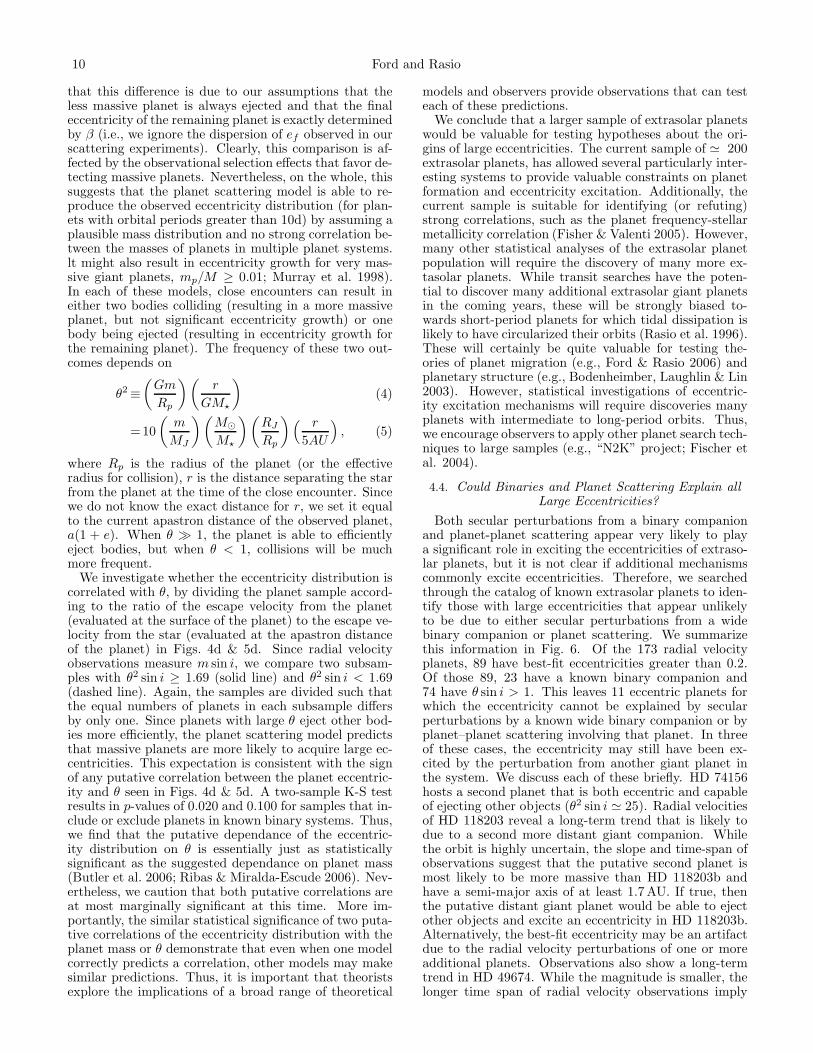
where Rp is the radius of the planet (or the effectiveradius for collision), r is the distance separating the starfrom the planet at the time of the close encounter. Sincewe do not know the exact distance for r, we set it equalto the current apastron distance of the observed planet,a(1 + e). When θ ≫ 1, the planet is able to efficientlyeject bodies, but when θ < 1, collisions will be muchmore frequent.

We investigate whether the eccentricity distribution iscorrelated with θ, by dividing the planet sample accord-ing to the ratio of the escape velocity from the planet(evaluated at the surface of the planet) to the escape ve-locity from the star (evaluated at the apastron distanceof the planet) in Figs. 4d & 5d. Since radial velocityobservations measure m sin i, we compare two subsam-ples with θ2 sin i ≥ 1.69 (solid line) and θ2 sin i < 1.69(dashed line). Again, the samples are divided such thatthe equal numbers of planets in each subsample differsby only one. Since planets with large θ eject other bod-ies more efficiently, the planet scattering model predictsthat massive planets are more likely to acquire large ec-centricities. This expectation is consistent with the signof any putative correlation between the planet eccentric-ity and θ seen in Figs. 4d & 5d. A two-sample K-S testresults in p-values of 0.020 and 0.100 for samples that in-clude or exclude planets in known binary systems. Thus,we find that the putative dependance of the eccentric-ity distribution on θ is essentially just as statisticallysignificant as the suggested dependance on planet mass(Butler et al. 2006; Ribas & Miralda-Escude 2006). Nev-ertheless, we caution that both putative correlations areat most marginally significant at this time. More im-portantly, the similar statistical significance of two puta-tive correlations of the eccentricity distribution with theplanet mass or θ demonstrate that even when one modelcorrectly predicts a correlation, other models may makesimilar predictions. Thus, it is important that theoristsexplore the implications of a broad range of theoretical

models and observers provide observations that can testeach of these predictions.

We conclude that a larger sample of extrasolar planetswould be valuable for testing hypotheses about the ori-gins of large eccentricities. The current sample of ≃ 200extrasolar planets, has allowed several particularly inter-esting systems to provide valuable constraints on planetformation and eccentricity excitation. Additionally, thecurrent sample is suitable for identifying (or refuting)strong correlations, such as the planet frequency-stellarmetallicity correlation (Fisher & Valenti 2005). However,many other statistical analyses of the extrasolar planetpopulation will require the discovery of many more ex-tasolar planets. While transit searches have the poten-tial to discover many additional extrasolar giant planetsin the coming years, these will be strongly biased to-wards short-period planets for which tidal dissipation islikely to have circularized their orbits (Rasio et al. 1996).These will certainly be quite valuable for testing the-ories of planet migration (e.g., Ford & Rasio 2006) andplanetary structure (e.g., Bodenheimber, Laughlin & Lin2003). However, statistical investigations of eccentric-ity excitation mechanisms will require discoveries manyplanets with intermediate to long-period orbits. Thus,we encourage observers to apply other planet search tech-niques to large samples (e.g., “N2K” project; Fischer etal. 2004).

4.4. Could Binaries and Planet Scattering Explain allLarge Eccentricities?

Both secular perturbations from a binary companionand planet-planet scattering appear very likely to playa significant role in exciting the eccentricities of extraso-lar planets, but it is not clear if additional mechanismscommonly excite eccentricities. Therefore, we searchedthrough the catalog of known extrasolar planets to iden-tify those with large eccentricities that appear unlikelyto be due to either secular perturbations from a widebinary companion or planet scattering. We summarizethis information in Fig. 6. Of the 173 radial velocityplanets, 89 have best-fit eccentricities greater than 0.2.Of those 89, 23 have a known binary companion and74 have θ sin i > 1. This leaves 11 eccentric planets forwhich the eccentricity cannot be explained by secularperturbations by a known wide binary companion or byplanet–planet scattering involving that planet. In threeof these cases, the eccentricity may still have been ex-cited by the perturbation from another giant planet inthe system. We discuss each of these briefly. HD 74156hosts a second planet that is both eccentric and capableof ejecting other objects (θ2 sin i ≃ 25). Radial velocitiesof HD 118203 reveal a long-term trend that is likely todue to a second more distant giant companion. Whilethe orbit is highly uncertain, the slope and time-span ofobservations suggest that the putative second planet ismost likely to be more massive than HD 118203b andhave a semi-major axis of at least 1.7 AU. If true, thenthe putative distant giant planet would be able to ejectother objects and excite an eccentricity in HD 118203b.Alternatively, the best-fit eccentricity may be an artifactdue to the radial velocity perturbations of one or moreadditional planets. Observations also show a long-termtrend in HD 49674. While the magnitude is smaller, thelonger time span of radial velocity observations imply

Eccentric Extrasolar Planets 11

that the putative planet most likely has an orbital pe-riod beyond 5 AU, so it too is likely able to eject otherobjects. GJ 876 contains three planets and the outertwo are participating in a 2:1 mean motion resonances.Detailed modeling of this system suggests that the ec-centricities of both GJ 876b and GJ 876c are likely dueto eccentricity excitation that occured due to convergentmigration and resonance capture (Lee & Peale 2002; Kleyet al. 2004). Technically, GJ 876c is massive enough toeject other bodies (θ2 sin i ≃ 1.2), so a hybrid scenario ofplanet scattering and resonant capture is possible (e.g.,Sandor & Kley 2005).

This leaves 7 out of 89 eccentric planets that cannot beexplained by secular perturbations from a known wide bi-nary or by planet–planet scattering by any planet whichis currently supported with radial velocity observations(HD 33283b, HD 108147b, HD 117618b, HD 208487b,HD 216770b, Hip 14810c), unless sin i ≪ 1. Of course,these systems may have an undetected binary compan-ion. For example, there is preliminary evidence for a bi-nary companion to HD 52265 (Chauvin et al. 2006), butfollow-up observations are needed to confirm this. Sim-ilarly, there may be additional undetected planets. Wenote that over half of these systems were discovered onlyin the last year, most have a relatively modest number ofradial velocity observations, and over half of these havea relatively modest signal-to-noise ratio (velocity semi-amplitude over the effective single measurement preci-sion).

Thus, there is a very real possibility that additional ra-dial velocity observations may result in revisions to themeasured eccentricity (e.g., GJ 436b), the detection of along-term trend most likely due to a distant giant planet,and/or the detection of additional planets. The uncer-tainties in the orbital elements can be particularly prob-lematic in cases where there is an undetected planet isnear a 2:1 or 3:1 mean motion resonance. Previous ex-perience has taught that the perturbations from yet un-detected planets can lead to significant overestimates ofthe eccentricity. We encourage additional observations ofthese systems, which may prove particularly interestingfor testing theories of eccentricity excitation. We notethat HD 108147, Hip 14810, HD 33283, HD 52265, andHD 216770 are particularly favorable, since they havevelocity amplitudes and eccentricities such that one ec-centric planet could be differentiated from two planetsin a mean motion resonance. We will present a more de-tailed discussion of resonant systems in a future paper.If future observations were to confirm the sizable eccen-tricity, the lack of other massive companions (both giantplanet and stellar companions), then these systems wouldprovide evidence for at least one additional eccentricityexcitation mechanism in addition to planet-planet scat-tering, secular perturbations from binaries, and resonantcapture.

5. CONCLUSIONS

A planetary system with two or more giant planetsmay become dynamically unstable, leading to a collisionor the ejection of one of the planets from the system.Early simulations for equal-mass planets revealed dis-crepancies between the results of numerical simulationsand the observed orbital elements of extrasolar planets.However, our new simulations for two planets with un-

equal masses show a reduced frequency of collisions ascompared to scattering between equal-mass planets andsuggest that the two-planet scattering model can repro-duce the observed eccentricities with a plausible distri-bution of planet mass ratios.

Additionally, the two-planet scattering model predictsa maximum eccentricity of ∼ 0.8, which is independentof the distribution of planet mass ratios. This predictedeccentricity limit compares favorably with current obser-vations and will be tested by future planet discoveries.The current sample of extrasolar planets provides hintsof a correlation between the eccentricity distribution andother properties. We show that the putative correlationbetween eccentricity distribution and the ratio of the es-cape velocity from the planet to the escape velocity fromthe star is comparable in statistical significance to theputative correlation between the eccentricity distributionand planet mass. Additionally, both correlations remainmarginally significant, when we exclude planets in knownbinary systems. We have identified a few particularly in-teresting planets that are unlikely to be explained bythe two-planet scattering model, since θ2 sin i < 1. Weencourage additional observations of these systems to de-termine if these are isolated planets or if there may beother planets in the system that could excite large ec-centricities and/or cause the current eccentricity to beoverestimated.

The combination of planet–planet scattering and tidalcircularization may be able to explain the existence ofgiant planets in very short period orbits. However, thepresence of giant planets at slightly larger orbital periods(small enough to require significant migration, but largeenough that tidal circularization is ineffective) is moredifficult to explain. Finally, the planet–planet scatteringmodel predicts a significant number of extremely looselybound and free floating giant planets, which may also beobservable (Lucas & Roche 2000; Zapatero Osorio et al.2002).

A complete theory of planet formation must explainboth the eccentric orbits prevalent among extrasolarplanets and the nearly circular orbits in the Solar Sys-tem. Despite significant uncertainties about giant planetformation, the leading models for the formation and earlydynamical evolution of the Solar System’s giant planetsagree that the giant planets in the Solar System wentthrough a phase of large eccentricities (Levison et al.1998; Thommes et al. 1999, 2002; Tsiganis et al. 2005;Ford & Chaing 2007). If Uranus and Neptune formedcloser to the Sun, then close encounters are necessaryto scatter them outwards to their current orbital dis-tances. During this phase, their eccentricities can exceed≃ 0.5 (Tsiganis et al. 2005). Alternatively, if Uranus andNeptune were able to form near their current locations,then oligarch growth predicts that several other ice giantsshould have formed contemporaneously in the region be-tween Uranus and Neptune (Goldreich, Lithwick & Sari2004). The scattering necessary to to remove these ex-tra ice giants would have excited sizable eccentricities inUranus and Neptune (Ford & Chaing 2007; Levison &Morbidelli 2007). Finally, the gravitational instabilitymodel predicts that most giant planets form with signifi-cant eccentricities (Boss 1995). Therefore, it seems mostlikely that even the giant planets in our Solar Systemwere once eccentric.

12 Ford and Rasio

Perhaps the question, “What mechanism excites theeccentricity of extrasolar planets?” should be replacedwith “What mechanism damps the eccentricities of giantplanets?” Unless giant planets form via gravitational in-stability, interactions with a gas disk are not an option,since the eccentricities would have been excited after thegas was cleared. Both dynamical friction within a plan-etesimal disk and planetesimal scattering could damp ec-centricities in both the Solar System and other planetarysystems. Dynamical friction alone would not clear thesmall bodies, so either accretion or ejection would berequired to satisfy observational constraints (Goldreich,Lithwick & Sari 2004). Planetesimal scattering providesa natural mechanism to simultaneously damp eccentric-ities and remove small bodies from planetary systems.

Perhaps, the key parameter that determines whether aplanetary system will have eccentric or nearly circularorbits is the amount of mass in planetesimals at the timeof the last strong planet-planet scattering event. Thiscould explain why more massive planets may tend tohave larger eccentricities. Additionally, the chaotic evo-lution of multiple planet systems naturally provides alarge dispersion in the time until dynamical instabilityresults in close encounters (Chambers, Wetherill & Boss1996; FHR; Marzari & Weidenschilling 2002). This could

explain why some planetary systems have large eccen-tricities (late stage instability when there was little diskto damp eccentricities), while our planets in the SolarSystem have nearly circular orbits (last instability oc-cured while sufficient planetesimal disk to damp eccen-tricities). Unfortunately, this model would significantlycomplicate the interpretation of the observed eccentricitydistribution for some extrasolar planets. Investigationsof dynamical instabilities in systems with three or moreplanets have only begun to explore the large availableparameter space. Future numerical investigations willbe necessary to test such theoretical models.

We thank E.I. Chiang, M. Holman, G. Laughlin, M.H.Lee, H. Levison, G.W. Marcy, A. Morbidelli, J.C.B. Pa-paloizou, S. Peale, and J. Wright for useful discussions.Support for E.B.F. was provided by a Miller ResearchFellowship and by NASA through Hubble Fellowshipgrant HST-HF-01195.01A awarded by the Space Tele-scope Science Institute, which is operated by the Associ-ation of Universities for Research in Astronomy, Inc., forNASA, under contract NAS 5-26555. This work was sup-ported by NSF grants AST–0206182 and AST–0507727at Northwestern University.

REFERENCES

Adams, F. C., & Laughlin, G. 2003, Icarus, 163, 290Adams, F. C., & Laughlin, G. 2006, ApJ, 649, 1004Artymowicz 1992 PASP 104, 769.Artymowicz 1993 ApJ 419, 116.Barnes, R., & Greenberg, R. 2006, ApJ, 638, 478Barnes, R., & Greenberg, R. 2006, ApJ, 647, L163Barnes, R. Qunn, T. 2004 ApJ 611, 494.Bate, M.R., Lubow, S.H., Ogilvie, G.I., Miller, K.A. 2003 MNRAS

341, 213.Black, D. C. 1997, ApJ, 490, L171Bodenheimer, P., Laughlin, G., & Lin, D. N. C. 2003, ApJ, 592,

555Boss, A.P. 1995 Science, 267, 360.Butler, R. P., et al. 2006, ApJ, 646, 505Chambers, J. E. 1999, MNRAS, 304, 793Chambers, J.E., Wetherill, G.W. & Boss, A.P. 1996 Icarus 119,

261.Chatterjee, S., Ford, E.B., Rasio, F.A. 2007, ApJ, submitted.

[arxiv:astro-ph/0703166]Chauvin, G., Lagrange, A.-M., Udry, S., Fusco, T., Galland, F.,

Naef, D., Beuzit, J.-L., & Mayor, M. 2006, A&A, 456, 1165Chiang, E.I. 2003 ApJ 584, 465.Chiang, E.I. & Murray, N. 2002 ApJ 576, 473.D’Angelo, G., Kley, W, Henning, T. 2003 ApJ 586, 540.Desidera, S., & Barbieri, M. 2006, ArXiv Astrophysics e-prints,

arXiv:astro-ph/0610623Faber, J.A., Rasio, F.A. & Willems, B. 2005 Icarus, 175, 248Fischer, D. A., et al. 2005, ApJ, 620, 481Ford, E. B. 2005, AJ, 129, 1706Ford, E. B. 2006, ApJ, 642, 505 Orbits of Extrasolar PlanetsFord, E.B. & Chaing, E.I. 2007, ApJ, in press.

[ariv:astro-ph/0701745]Ford, E.B. & Gaudi, B.S. 2006, ApJ, 652, L137.Ford, E.B., Havlickova, M. & Rasio, F.A. 2001 Icarus 150, 303.Ford, E.B. & Holman, M. 2007 in preparation.Ford, E.B., Kozinsky, B., Rasio, F.A. 2000 ApJ 535, 385.Ford, E.B., Lystad, V., Rasio, F.A. 2005 Nature 434, 873.Ford, E.B. & Rasio, F.A. 2006, ApJ, 638, L45.Ford, E.B., Rasio, F.A., Yu, K. 2003 Scientific Frontiers in Research

on Extrasolar Planets, eds. D. Deming & S. Seager (ASPConference Series, 294), 181.

Gaudi, B.S. & Winn, J.N. 2007, ApJ 655, 550.Gladman, B. 1993 Icarus, 106, 247.Goldreich, P., Lithwick, Y., Sari, R. 2004 ApJ 614, 497.Goldreich, P., Sari, R. 2003 ApJ 585, 1024.

Goldreich, P., Tremaine, S. 1979 ApJ 233, 857.Goldreich, P., Tremaine, S. 1980 ApJ 241, 425.Gregory, P. C. 2005, ApJ, 631, 1198Gregory, P. C. 2006, MNRAS, 1375Halbwachs, J.L., Mayor, M., Udry, S. 2005 A&A 431, 1129.Holman, M., Touma, J., Tremaine, S. 1997 Nature 386, 254.Hurley, J. R., & Shara, M. M. 2002, ApJ, 565, 1251Johnson, J. A., et al. 2006, ApJ, 647, 600Jones, H. R. A., Butler, R. P., Tinney, C. G., Marcy, G. W., Carter,

B. D., Penny, A. J., McCarthy, C., & Bailey, J. 2006, MNRAS,369, 249

Juric, M. & Tremaine, S. 2007, submitted to ApJ.[arxiv:astro-ph/0703160]

Kley, W. 2000 MNRAS 313, L47.Kley, W., Lee, M.H., Murray, N., Peale, S.J. 2005 A&A 437, 727.Kley, W., Peitz, J. & Bryden, G. 2004 A&A, 414, 735.Kley, W., Lee, M. H., Murray, N., & Peale, S. J. 2005, A&A, 437,

727Kokubo, E. & Ida, S. 1998a Icarus 123, 180.Kokubo, E. & Ida, S. 1998b Icarus 131, 171.Laughlin, G., & Adams, F. C. 1998, ApJ, 508, L171Lee, M.H. & Peale, S.J. 2002 ApJ 567, 596.Lee, M.H. & Peale, S.J. 2003 ApJ 592, 1201.Levison, H.F., Lissuaer, J.J., Duncan, M.J. 1998 AJ 116, 1998.Lin, D.N.C. & Ida, S. 1997 ApJ, 447, 781Lissauer, J.J. 1993 ARAA, 31, 129Lissauer, J.J. 1995 Icarus 114, 217.Malmberg, D. et al. 2007 submitted to MNRAS

[arxiv:astro-ph/0702524]Marzari, F., & Weidenschilling, S. J. 2002, Icarus, 156, 570Marzari, F., Weidenschilling, S. J., Barbieri, M., & Granata, V.

2005, ApJ, 618, 502Mazeh, T., Krymolowski, Y., Rosenfield, G. 1997, ApJ, 447, L103.Murray, N. Hansen, B., Holman, M., Tremaine, S. 1998 Science

279, 69.Murray-Clay, R.A. Chiang, E.I. 2007, in preparation.Naef, D., et al. 2001, A&A, 375, L27Nagasawa, M., Lin, D.N.C., Ida, S. 2003 ApJ 586, 1374.Namouni, F., & Zhou, J. L. 2006, Celestial Mechanics and

Dynamical Astronomy, 95, 245Namouni, F. 2005, AJ, 130, 280Narita, N. et al. 2007 PASJ, submitted [arxiv:astro-ph/0702707]Ogilvie & Lubow 2003 ApJ 587, 398.Papaloizou, J.C.B. & Terquem, C. 2001 MNRAS 325, 221.Papaloizou, J.C.B. & Terquem, C. 2002 MNRAS 332, L39.

Eccentric Extrasolar Planets 13

TABLE 1Orbital Elements of Remaining Planet Following an Ejection

m1 = m< m2 = m> combinedm</M m>/M

˙

af

¸

σaf

˙

af

¸

σaf

˙

ef

¸

σef

˙

if¸

σif

(◦) (◦)

0.0012 0.0048 0.933 0.010 0.813 0.006 0.202 0.056 1.93 1.100.0015 0.0045 0.888 0.009 0.779 0.005 0.263 0.071 1.99 1.220.0018 0.0042 0.828 0.030 0.736 0.047 0.333 0.100 2.22 1.840.0021 0.0039 0.749 0.076 0.677 0.083 0.421 0.133 2.94 3.260.0024 0.0036 0.670 0.079 0.618 0.085 0.513 0.145 3.80 4.760.0027 0.0033 0.595 0.054 0.577 0.053 0.602 0.142 4.23 3.230.0030 0.0030 0.570 0.007 0.570 0.053 0.624 0.135 4.27 3.46

Papalouizou, J.C.B., Nelson, R.P. & Masset, F. 2001 A&A 366,263.

Pfahl, E. & Muterspaugh, M. 2006 ApJ, 652, 1694.Pollack, J.B., Hubickyj, O., Bodenheimer, P., Lissauer, J.J.,

Podolak, M. & Greenzweig, Y. 1996 Icarus 124, 62.Pont, F., & Eyer, L. 2004, MNRAS, 351, 487Portegies Zwart, S.F. & McMillan, S.L.W. 2005 ApJ 633, 141.Rasio, F.A. & Ford, E.B. 1996 Science 274, 954.Rasio, F.A., Tout, C.A., Lubow, S.H. & Livio, M. 1996 ApJ, 470,

1187.Rauch, K. P., & Holman, M. 1999, AJ, 117, 1087Ribas, I., & Miralda-Escude, J. 2006, ArXiv Astrophysics e-prints,

arXiv:astro-ph/0606009Sandor, Z., & Kley, W. 2006, A&A, 451, L31Stepinsky, T.F. & Black, D.C. 2000, A&A, 356, 903Stepinsky, T.F., Malhotra, R., & Black, D.C. 2000 ApJ 545, 1004.Takeda, G., & Rasio, F. A. 2005, ApJ, 627, 1001Takeda, G., & Rasio, F. A. 2006, Ap&SS, 19Thommes, E. W., Duncan, M. J., & Levison, H. F. 1999, Nature,

402, 635Thommes, E. W., Duncan, M. J., & Levison, H. F. 2002, AJ, 123,

2862

Trilling, D. E., Benz, W., Guillot, T., Lunine, J. I., Hubbard, W. B.,& Burrows, A. 1998, ApJ, 500, 428

Tsiganis, K., Gomes, R., Morbidelli, A., Levison, H.F. 2005 Nature435, 459.

Veras, D. Armitage, P.J. 2004 Icarus 172, 349.Veras, D. Armitage, P.J. 2005 ApJ, 620, L111.Veras, D. Armitage, P.J. 2006 ApJ, 645, 1509.Vidal-Madjar, A., Lecavelier des Etangs, A., Desert, J.-M.,

Ballester, G. E., Ferlet, R., Hebrard, G., & Mayor, M. 2003,Nature, 422, 143

Weidenschillingm S.J. & Marzari, F. 1996 Nature 384, 619.Wisdom, J., & Holman, M. 1991, AJ, 102, 1528Wolf, S., Laughlin, G., Henry, G., Fischer, D.A., Marcy, G.W.,

Butler, R.P., Vogt, S. 2007, ApJ, in press.Wright, J. T., et al. 2006, ArXiv Astrophysics e-prints,

arXiv:astro-ph/0611658Yu, Q., & Tremaine, S. 2001, AJ, 121, 1736Zakamska, N.L., Tremaine, S. 2004 128, 869.

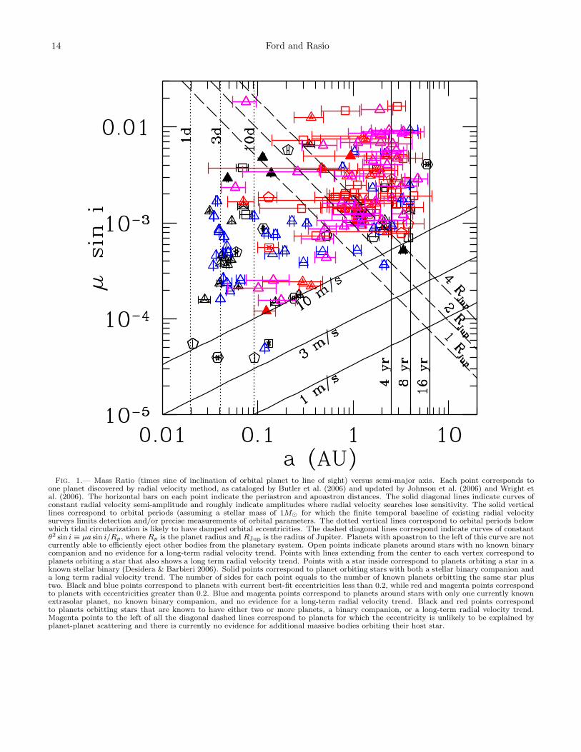
14 Ford and Rasio

Fig. 1.— Mass Ratio (times sine of inclination of orbital planet to line of sight) versus semi-major axis. Each point corresponds toone planet discovered by radial velocity method, as cataloged by Butler et al. (2006) and updated by Johnson et al. (2006) and Wright etal. (2006). The horizontal bars on each point indicate the periastron and apoastron distances. The solid diagonal lines indicate curves ofconstant radial velocity semi-amplitude and roughly indicate amplitudes where radial velocity searches lose sensitivity. The solid verticallines correspond to orbital periods (assuming a stellar mass of 1M⊙ for which the finite temporal baseline of existing radial velocitysurveys limits detection and/or precise measurements of orbital parameters. The dotted vertical lines correspond to orbital periods belowwhich tidal circularization is likely to have damped orbital eccentricities. The dashed diagonal lines correspond indicate curves of constantθ2 sin i ≡ µa sin i/Rp, where Rp is the planet radius and RJup is the radius of Jupiter. Planets with apoastron to the left of this curve are notcurrently able to efficiently eject other bodies from the planetary system. Open points indicate planets around stars with no known binarycompanion and no evidence for a long-term radial velocity trend. Points with lines extending from the center to each vertex correspond toplanets orbiting a star that also shows a long term radial velocity trend. Points with a star inside correspond to planets orbiting a star in aknown stellar binary (Desidera & Barbieri 2006). Solid points correspond to planet orbiting stars with both a stellar binary companion anda long term radial velocity trend. The number of sides for each point equals to the number of known planets orbitting the same star plustwo. Black and blue points correspond to planets with current best-fit eccentricities less than 0.2, while red and magenta points correspondto planets with eccentricities greater than 0.2. Blue and magenta points correspond to planets around stars with only one currently knownextrasolar planet, no known binary companion, and no evidence for a long-term radial velocity trend. Black and red points correspondto planets orbitting stars that are known to have either two or more planets, a binary companion, or a long-term radial velocity trend.Magenta points to the left of all the diagonal dashed lines correspond to planets for which the eccentricity is unlikely to be explained byplanet-planet scattering and there is currently no evidence for additional massive bodies orbiting their host star.

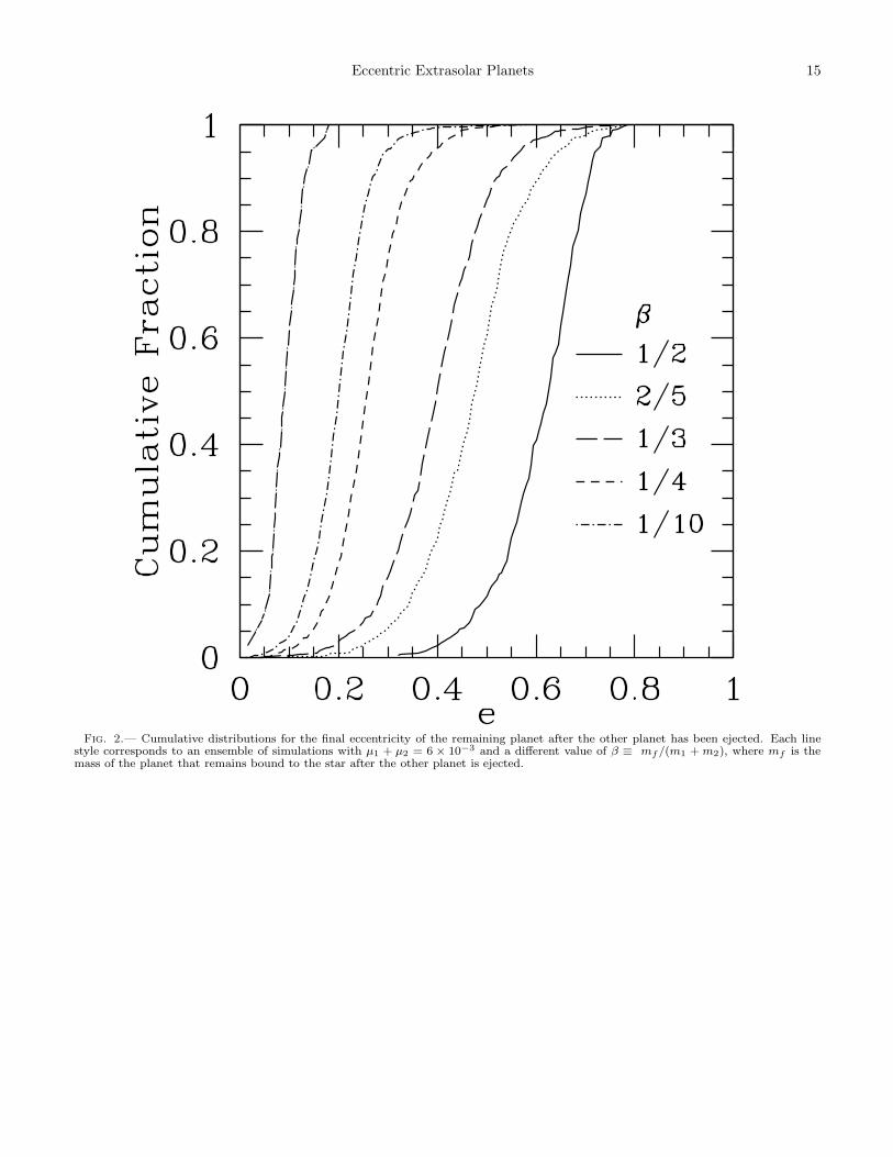
Eccentric Extrasolar Planets 15

Fig. 2.— Cumulative distributions for the final eccentricity of the remaining planet after the other planet has been ejected. Each linestyle corresponds to an ensemble of simulations with µ1 + µ2 = 6 × 10−3 and a different value of β ≡ mf /(m1 + m2), where mf is themass of the planet that remains bound to the star after the other planet is ejected.

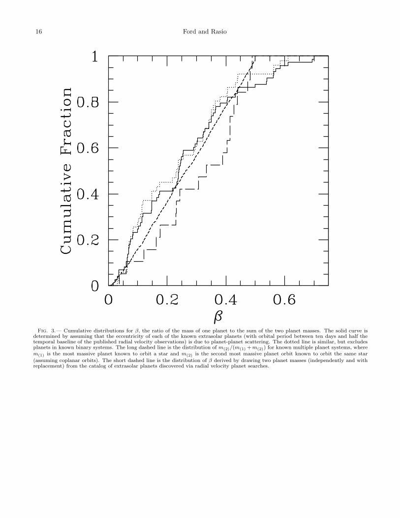
16 Ford and Rasio

Fig. 3.— Cumulative distributions for β, the ratio of the mass of one planet to the sum of the two planet masses. The solid curve isdetermined by assuming that the eccentricity of each of the known extrasolar planets (with orbital period between ten days and half thetemporal baseline of the published radial velocity observations) is due to planet-planet scattering. The dotted line is similar, but excludesplanets in known binary systems. The long dashed line is the distribution of m(2)/(m(1) +m(2)) for known multiple planet systems, wherem(1) is the most massive planet known to orbit a star and m(2) is the second most massive planet orbit known to orbit the same star

(assuming coplanar orbits). The short dashed line is the distribution of β derived by drawing two planet masses (independently and withreplacement) from the catalog of extrasolar planets discovered via radial velocity planet searches.

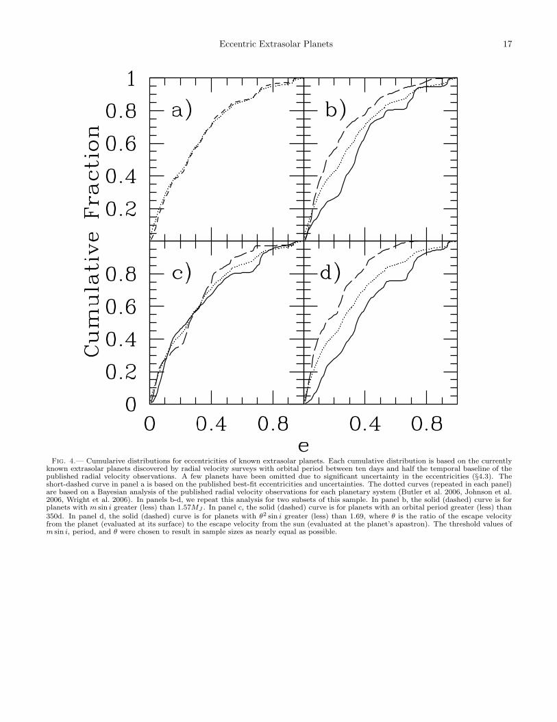
Eccentric Extrasolar Planets 17

Fig. 4.— Cumularive distributions for eccentricities of known extrasolar planets. Each cumulative distribution is based on the currentlyknown extrasolar planets discovered by radial velocity surveys with orbital period between ten days and half the temporal baseline of thepublished radial velocity observations. A few planets have been omitted due to significant uncertainty in the eccentricities (§4.3). Theshort-dashed curve in panel a is based on the published best-fit eccentricities and uncertainties. The dotted curves (repeated in each panel)are based on a Bayesian analysis of the published radial velocity observations for each planetary system (Butler et al. 2006, Johnson et al.2006, Wright et al. 2006). In panels b-d, we repeat this analysis for two subsets of this sample. In panel b, the solid (dashed) curve is forplanets with m sin i greater (less) than 1.57MJ . In panel c, the solid (dashed) curve is for planets with an orbital period greater (less) than350d. In panel d, the solid (dashed) curve is for planets with θ2 sin i greater (less) than 1.69, where θ is the ratio of the escape velocityfrom the planet (evaluated at its surface) to the escape velocity from the sun (evaluated at the planet’s apastron). The threshold values ofm sin i, period, and θ were chosen to result in sample sizes as nearly equal as possible.

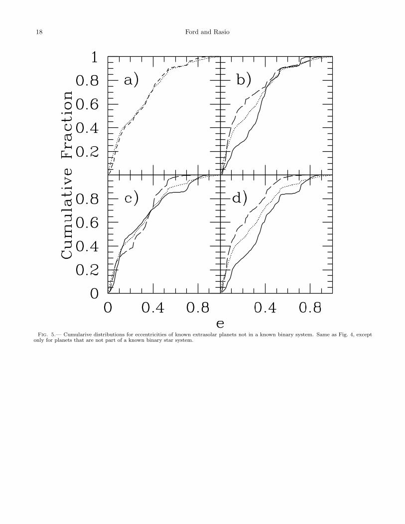
18 Ford and Rasio

Fig. 5.— Cumularive distributions for eccentricities of known extrasolar planets not in a known binary system. Same as Fig. 4, exceptonly for planets that are not part of a known binary star system.

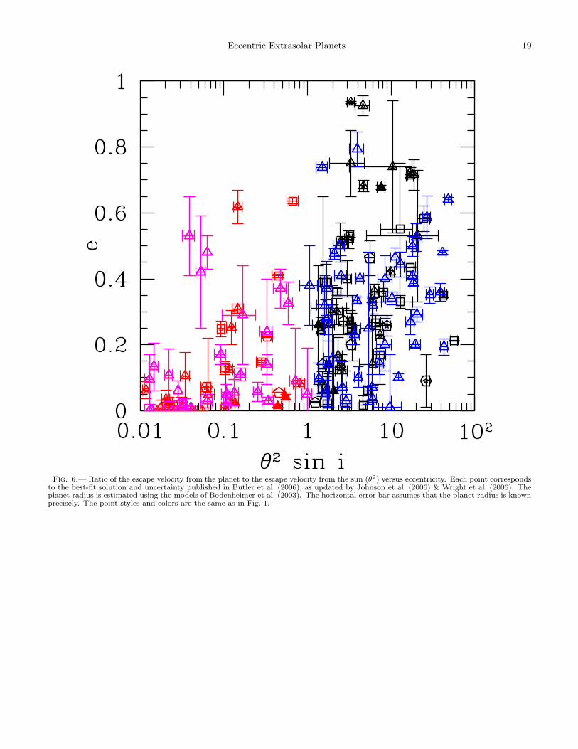
Eccentric Extrasolar Planets 19

Fig. 6.— Ratio of the escape velocity from the planet to the escape velocity from the sun (θ2) versus eccentricity. Each point correspondsto the best-fit solution and uncertainty published in Butler et al. (2006), as updated by Johnson et al. (2006) & Wright et al. (2006). Theplanet radius is estimated using the models of Bodenheimer et al. (2003). The horizontal error bar assumes that the planet radius is knownprecisely. The point styles and colors are the same as in Fig. 1.