Embed Size (px)
Citation preview
Retrospective Theses and Dissertations Iowa State University Capstones, Theses andDissertations
2007
Applications of asymptotic expansions to somestatistical problemsArindam ChatterjeeIowa State University
Follow this and additional works at: https://lib.dr.iastate.edu/rtd
Part of the Statistics and Probability Commons
This Dissertation is brought to you for free and open access by the Iowa State University Capstones, Theses and Dissertations at Iowa State UniversityDigital Repository. It has been accepted for inclusion in Retrospective Theses and Dissertations by an authorized administrator of Iowa State UniversityDigital Repository. For more information, please contact [email protected].
Recommended CitationChatterjee, Arindam, "Applications of asymptotic expansions to some statistical problems" (2007). Retrospective Theses andDissertations. 15993.https://lib.dr.iastate.edu/rtd/15993

Applications of asymptotic expansions to some statistical problems
by
Arindam Chatterjee
A dissertation submitted to the graduate faculty
in partial fulfillment of the requirements for the degree of
DOCTOR OF PHILOSOPHY
Major: Statistics
Program of Study Committee:Soumendra N. Lahiri, Co-major Professor
Tapabrata Maiti, Co-major ProfessorMichael D. LarsenDaniel J. NordmanSunder Sethuraman
Iowa State University
Ames, Iowa
2007
Copyright c© Arindam Chatterjee, 2007. All rights reserved.

UMI Number: 3274822
32748222007
UMI MicroformCopyright
All rights reserved. This microform edition is protected against unauthorized copying under Title 17, United States Code.
ProQuest Information and Learning Company 300 North Zeeb Road
P.O. Box 1346 Ann Arbor, MI 48106-1346
by ProQuest Information and Learning Company.

ii
TABLE OF CONTENTS
LIST OF TABLES . . . . . . . . . . . . . . . . . . . . . . . . . . . . . . . . . . . . . . . . iv
LIST OF FIGURES . . . . . . . . . . . . . . . . . . . . . . . . . . . . . . . . . . . . . . . v
ACKNOWLEDGEMENTS . . . . . . . . . . . . . . . . . . . . . . . . . . . . . . . . . . . vi
INTRODUCTION . . . . . . . . . . . . . . . . . . . . . . . . . . . . . . . . . . . . . . . . 1
A BERRY-ESSEEN THEOREM FOR HYPERGEOMETRIC PROBABILITIES
UNDER MINIMAL CONDITIONS . . . . . . . . . . . . . . . . . . . . . . . . . . . 3
Abstract . . . . . . . . . . . . . . . . . . . . . . . . . . . . . . . . . . . . . . . . . . . . . . . . 3
1 Introduction . . . . . . . . . . . . . . . . . . . . . . . . . . . . . . . . . . . . . . . . . . . 3
2 Theoretical Results . . . . . . . . . . . . . . . . . . . . . . . . . . . . . . . . . . . . . . . 5
3 Proofs . . . . . . . . . . . . . . . . . . . . . . . . . . . . . . . . . . . . . . . . . . . . . . 7
NORMAL APPROXIMATION TO THE HYPERGEOMETRIC DISTRIBUTION
IN NONSTANDARD CASES AND A SUB-GAUSSIAN BERRY-ESSEEN THE-
OREM . . . . . . . . . . . . . . . . . . . . . . . . . . . . . . . . . . . . . . . . . . . . . 14
Abstract . . . . . . . . . . . . . . . . . . . . . . . . . . . . . . . . . . . . . . . . . . . . . . . . 14
1 Introduction . . . . . . . . . . . . . . . . . . . . . . . . . . . . . . . . . . . . . . . . . . . 14
2 Main Results . . . . . . . . . . . . . . . . . . . . . . . . . . . . . . . . . . . . . . . . . . 17
3 Numerical results . . . . . . . . . . . . . . . . . . . . . . . . . . . . . . . . . . . . . . . . 19
4 Proofs . . . . . . . . . . . . . . . . . . . . . . . . . . . . . . . . . . . . . . . . . . . . . . 22
ASYMPTOTIC PROPERTIES OF SAMPLE QUANTILES FROM A FINITE POP-
ULATION . . . . . . . . . . . . . . . . . . . . . . . . . . . . . . . . . . . . . . . . . . . 42
Abstract . . . . . . . . . . . . . . . . . . . . . . . . . . . . . . . . . . . . . . . . . . . . . . . . 42
1 Introduction . . . . . . . . . . . . . . . . . . . . . . . . . . . . . . . . . . . . . . . . . . . 42
2 Main Results . . . . . . . . . . . . . . . . . . . . . . . . . . . . . . . . . . . . . . . . . . 43
3 Bootstrap . . . . . . . . . . . . . . . . . . . . . . . . . . . . . . . . . . . . . . . . . . . . 44

iii
4 Proofs . . . . . . . . . . . . . . . . . . . . . . . . . . . . . . . . . . . . . . . . . . . . . . 46
4.1 Auxiliary Results . . . . . . . . . . . . . . . . . . . . . . . . . . . . . . . . . . . . 46
4.2 Proofs of the main results . . . . . . . . . . . . . . . . . . . . . . . . . . . . . . . 52
EDGEWORTH EXPANSIONS FOR SPECTRAL DENSITY ESTIMATES . . . . . 62
Abstract . . . . . . . . . . . . . . . . . . . . . . . . . . . . . . . . . . . . . . . . . . . . . . . . 62
1 Introduction . . . . . . . . . . . . . . . . . . . . . . . . . . . . . . . . . . . . . . . . . . . 62
2 Conditions for the Edgeworth Expansion . . . . . . . . . . . . . . . . . . . . . . . . . . . 64
2.1 Theoretical framework and general conditions . . . . . . . . . . . . . . . . . . . . 64
2.2 Sufficient conditions for linear processes . . . . . . . . . . . . . . . . . . . . . . . 66
3 Edgeworth Expansion for the Spectral Density Function . . . . . . . . . . . . . . . . . . 67
3.1 Density of the Edgeworth Expansion . . . . . . . . . . . . . . . . . . . . . . . . . 67
3.2 Main Results . . . . . . . . . . . . . . . . . . . . . . . . . . . . . . . . . . . . . . 69
4 Proofs . . . . . . . . . . . . . . . . . . . . . . . . . . . . . . . . . . . . . . . . . . . . . . 70
BIBLIOGRAPHY . . . . . . . . . . . . . . . . . . . . . . . . . . . . . . . . . . . . . . . . 76

iv
LIST OF TABLES
Table 1 Error of Normal approximation to Hypergeometric at N = 200 . . . . . . . . . 15
Table 2 Errors of Normal approximation for Hypergeometric and Binomial: N = 60 . . 20
Table 3 Errors of Normal approximation for Hypergeometric and Binomial: N = 200 . . 20
Table 4 Errors of Normal approximation for Hypergeometric and Binomial: N = 500 . . 21
Table 5 Errors of Normal approximation for Hypergeometric and Binomial: N = 2000 . 21
Table 6 Values of c(N, p, f) for N = 60, p, f ∈ .5, .6, .7, .8, .9. . . . . . . . . . . . . . . 22
Table 7 Values of c(N, p, f) for N = 200, p, f ∈ .5, .6, .7, .8, .9. . . . . . . . . . . . . . 23
Table 8 Values of c(N, p, f) for N = 500, p, f ∈ .5, .6, .7, .8, .9. . . . . . . . . . . . . . 23
Table 9 Values of c(N, p, f) for N = 2000, p, f ∈ .5, .6, .7, .8, .9. . . . . . . . . . . . . 23
v
LIST OF FIGURES
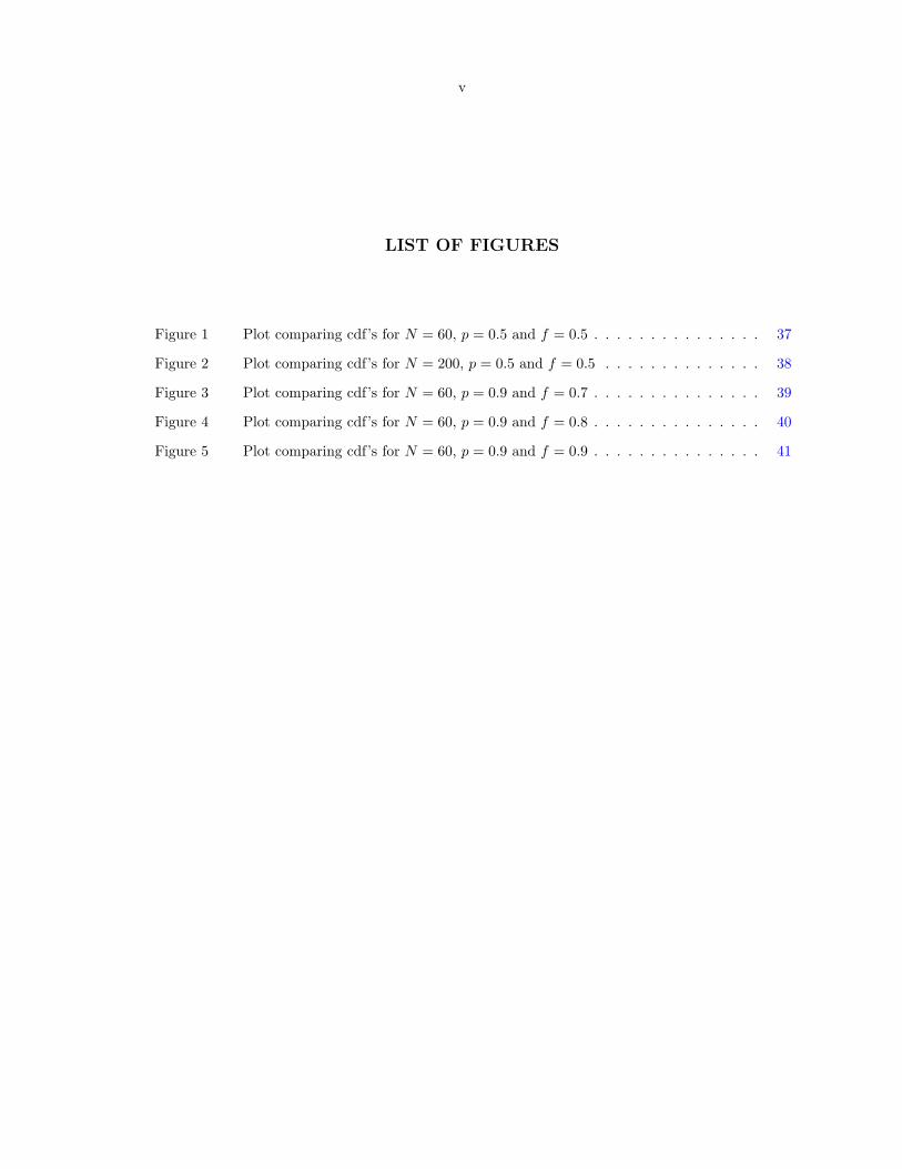
Figure 1 Plot comparing cdf’s for N = 60, p = 0.5 and f = 0.5 . . . . . . . . . . . . . . . 37
Figure 2 Plot comparing cdf’s for N = 200, p = 0.5 and f = 0.5 . . . . . . . . . . . . . . 38
Figure 3 Plot comparing cdf’s for N = 60, p = 0.9 and f = 0.7 . . . . . . . . . . . . . . . 39
Figure 4 Plot comparing cdf’s for N = 60, p = 0.9 and f = 0.8 . . . . . . . . . . . . . . . 40
Figure 5 Plot comparing cdf’s for N = 60, p = 0.9 and f = 0.9 . . . . . . . . . . . . . . . 41

vi
ACKNOWLEDGEMENTS
I would like to thank my advisers Professor Soumendra N. Lahiri and Professor Tapabrata Maiti
for their guidance, help, encouragement and support throughout my days as a graduate student. The
completion of my dissertation would have been impossible without their kind help and guidance.
I would also like to thank the members of my POS committee: Professor Michael D. Larsen, Professor
Daniel J. Nordman and Prof. Jiyeon Suh for finding time to serve and for their guidance and help. I
would also thank my ex-committee member Professor Sunder Sethuraman, who was unable to continue
until the end of my dissertation. Prof. Suh agreed to serve in my committee in the absence of Prof.
Sethuraman, and I specially thank her for this help.
I am also grateful to the Center for Survey Statistics and Methodology (CSSM) and the Department
of Statistics at Iowa State University for providing me an excellent learning environment and for their
financial assistance and support through out my stay at Iowa State. I would also thank the Department
of Statistics at Texas A&M University for their assistance and financial support throughout the last
year, during my stay in Texas A&M as a visiting student.
I am grateful to my teachers in Department of Statistics at University of Calcutta and specially to
Professor Gaurangadeb Chatterjee and Professor Tathagata Banerjee, who inspired me to take up a
research career in Statistics. My friends, who supported, helped and encouraged me through all the
good and bad times deserve my thanks.
Last but not the least, my parents deserves the greatest thanks for supporting me and for being my
source of strength and happiness.
1
INTRODUCTION
The dissertation is composed of four research papers. In all the papers asymptotic methods and
techniques are the main tools used to reach conclusions.
[1] A Berry-Esseen theorem for Hypergeometric probabilities under minimal conditions.
[2] Normal Approximation to the Hypergeometric distribution in nonstandard cases and a sub-
Gaussian Berry-Esseen Theorem.
[3] Asymptotic properties of sample quantiles from a finite population.
[4] Edgeworth expansions for Spectral density estimates.
The paper [1] considers the problem of Normal approximation to the Hypergeometric probabilities
under non-standard cases. From a dichotomous population of size N , containing M objects of type-A
and N −M objects of type-B, a simple random sample of size n is selected without replacement. Let
X be the number of type-A objects in the sample selected. Then X has a Hypergeometric distribution
with parameters (n,M,N). Let p = MN and f = n
N denote the population proportion of type-A objects
and the sampling fraction respectively. It is common to approximate the Hypergeometric distribution
with a corresponding Normal distribution when the parameters p and f are bounded away from 0 and
1. But, in the non-standard cases, these parameters take values close to 0 and 1. Though the non-
standard cases arise frequently, the validity and accuracy of normal approximations are not well studied
in these situations. In this paper we derive necessary and sufficient conditions on the finite population
parameters for a valid normal approximation. Solely under these conditions we obtain upper and lower
bounds on the difference between the Hypergeometric and Normal distribution.
In the paper [2], we consider the same set-up as in paper [1]. In this paper, a non-uniform Berry-
Esseen theorem for the Hypergeometric distribution is proved and it shows that the rate of Normal
approximation to the Hypergeometric can be considerably slower than the Binomial. As a consequence
of this result, a sub-exponential bound on the tail probabilities of the hypergeometric distribution are

2
obtained. We also obtain some numerical results that provide guidelines for using the Normal approxi-
mation to Hypergeometric distribution in finite samples.
The paper [3] considers the problem of estimation of quantiles from a finite population. As in pa-
pers [1] and [2], the sample is selected without replacement from the finite population. The asymptotic
results are derived under a superpopulation framework. We show that the sample quantile is asymptot-
ically normal and the scaled variance of the sample quantile converges to the asymptotic variance under
a slight moment condition. The performance of bootstrap in this case is also considered. We show that
Gross (1980)’s bootstrap method fails in this case, but a suitably modified version of the bootstrapped
quantile converges in distribution to the same asymptotic distribution as the sample quantile. Consis-
tency of the modified bootstrap variance estimate is also proved under the same moment conditions.
The paper [4] considers a different problem from the earlier three. This paper considers the problem
of Edgeworth expansion of spectral density estimators of a stationary time series. The spectral density
estimate at each frequency λ is based on tapered periodograms of overlapping blocks of observations.
We give conditions for the validity of a general order Edgeworth expansion under an approximate strong
mixing condition on the random variables, and also establish a moderate deviation inequality. We also
verify the conditions explicitly for linear time series, which are satisfied under mild and easy-to-check
conditions on the innovation variables and on their nonrandom co-efficients. The work makes use of
the results of Lahiri (2007) where general order Edgeworth expansions for functions of blocks of weakly
dependent random variables are derived. In our work we relax the assumption of Gaussianity, which
was used by Velasco and Robinson (2001) to obtain similar Edgeworth expansions.

3
A BERRY-ESSEEN THEOREM FOR HYPERGEOMETRIC
PROBABILITIES UNDER MINIMAL CONDITIONS
A paper published in the Proceedings of the American Mathematical Society1
Soumendra N. Lahiri and Arindam Chatterjee
Abstract
In this paper, we consider simple random sampling without replacement from a dichotomous finite
population and derive a necessary and sufficient condition on the finite population parameters for a
valid large sample Normal approximation to Hypergeometric probabilities. We then obtain lower and
upper bounds on the difference between the Normal and the Hypergeometric distributions solely under
this necessary and sufficient condition.
1 Introduction
Consider a dichotomous finite population of size N having M individuals of ‘type A’ and N −M
individuals of ‘type B’. Suppose a sample of size n is drawn at random, without replacement from this
population. Let X denote the number of ‘type A’-individuals in the sample. Then, X is said to have the
Hypergeometric distribution with parameters n,M,N , written as X ∼ Hyp(n;M,N). The probability
mass function (p.m.f) of X is given by,
P (X = x) ≡ P (x;n,M,N) =
(M
x )(N−Mn−x )
(Nn) if x = 0, 1 . . . , n
0 otherwise,(1.1)
where, for any two integers r ≥ 1 and s,(r
s
)=
r!
s!(r−s)! if 0 ≤ s ≤ r
0 otherwise,(1.2)
1available at http://www.ams.org/proc/2007-135-05/S0002-9939-07-08676-5/home.html

4
with 0! = 1 and r! = 1 · 2 · · · r. Let f = nN denote the sampling fraction and let p = M
N denote
the proportion of the ‘type A’-objects in the population. The Hypergeoemetric distribution plays an
important role in many areas of statistics, including sample surveys (Burstein (1975) and Wendell and
Schmee (1996)), capture-recapture methods (Seber (1970) and Wittes (1972)), analysis of contingency
tables Blyth and Staudte (1997), statistical quality control (Patel and Samaranayake (1991) and Sohn
(1997)), etc. Normal approximations to the Hypergeometric probabilities P (.;n,M,N) of (1.1) are
classical in the cases where the sampling fraction f and the proportion p are bounded away from 0 and
1; see, for example, Feller (1971). The nonstandard cases correspond to the extremes where f or p take
values near the boundary values 0 and 1. Although the nonstandard cases arise frequently in all these
areas of applications, the validity and accuracy of the Normal approximation in such situations are not
well studied. This paper is devoted to investigating the behavior of Normal approximation for both
standard and nonstandard cases.
The main results of the paper give a necessary and sufficient condition on the parameters f and p
for a valid Normal approximation. It is shown that a Normal limit for properly centered and scaled
version of X holds if and only if
Np(1− p)f(1− f) −→∞. (1.3)
As a consequence of this, we conclude that for the Normal distribution function to approximate the
distribution function of X, all four quantities, namely, (i) the number M (= Np) of ‘type A’-objects,
(ii) the number of ‘type B’-objects, N −M , (iii) the sample size n, as well as (iv) the size of the unse-
lected objects N − n in the population, must tend to infinity. We next investigate the rate of Normal
approximation to the distribution of X. Note that X is the sum of a collection of n dependent Bernoulli
random variables. In Section 2, we establish a Berry-Esseen Theorem on the rate of Normal approx-
imation to the distribution function of X solely under the necessary and sufficient condition (1.3). It
is shown that under (1.3) the rate of approximation is O([Np(1 − p)f(1 − f)]−1/2). It is also shown
in Section 2 that this rate is optimal in the sense that the (Kolmogorov) distance between the cdfs of
the Hypergeometric distribution and the Normal distribution is bounded below by a constant multiple
of [Np(1 − p)f(1 − f)]−1/2. Thus, the accuracy of Normal approximation necessarily deteriorates as
the factor Np(1− p)f(1− f) becomes small. In particular, for a given value of the population size N ,
the accuracy decreases as either p or f (or both) approach the boundary values 0 and 1. Note that the
rate O([Np(1− p)f(1− f)]−1/2) is equivalent to the standard rate O(n−1/2) (for sums of n independent
Bernoulli random variables, say) only when p is bounded away from 0 and 1 and f bounded away from
1. However, for p and f close to these boundary points, the rate of approximation can be substantially
5
slower. In such situations, the dependence of the Bernoulli random variables associated with X has a
nontrivial effect on the accuracy of the Normal approximation.
The rest of the paper is organized as follows. We conclude Section 1 with a brief literature review.
Section 2 introduces the asymptotic framework and contains the results on the validity of the Normal
approximation and the Berry-Esseen theorem. Proofs of all the results are given in Section 3. For
results on Normal approximations to Hypergeometric probabilities in the standard cases where the
sampling fraction f and the proportion p are bounded away from 0 and 1, see Feller (1971). For general
p and f , Nicholson (1956) derived some very precise bounds for the point probabilities P (.;n,M,N) (cf.
(1.1)) using some special normalizations of the Hypergeometric random variable X. General methods
for proving the CLT for sample means under sampling without replacement from finite populations are
given by Madow (1948), Erdos and Renyi (1959) and Hajek (1960). In relation to the earlier work, the
main contribution of our paper is to establish the theoretical validity of Normal approximation and the
Berry-Esseen Theorem under minimal conditions.
2 Theoretical Results
Let r be a positive integer valued variable and for each r ∈ N = 1, 2, . . ., let Xr be a random
variable having the Hypergeometric distribution with parameters (nr,Mr, Nr). Thus we consider a
sequence of dichotomous finite populations indexed by r, with the population of objects of type A and
the sampling fraction respectively given by,
pr =Mr
Nrand fr =
nr
Nrfor all r ∈ N. (2.1)
To avoid trivialities, all through the paper, we shall assume that for all r ∈ N,
1 ≤Mr < Nr, 1 ≤ nr < Nr, and N−1r = o (1) r →∞. (2.2)
Thus, pr , fr ∈ (0, 1) for all r ∈ N. Let
σ2r ≡ Nrprqrfr(1− fr), (2.3)
where qr = 1−pr. The first result concerns the validity of the Normal approximation to the distribution
of Xr.
Theorem 2.1. Suppose that (2.2) holds and that Xr ∼ Hyp(nr,Mr, Nr), r ∈ N. Then there exists a

6
Normal random variable W ∼ N(µ, σ2) for some µ ∈ R and σ ∈ (0,∞) such that
∆r ≡ supx∈R
∣∣∣∣P (Xr − nrpr
σr≤ x
)− P (W ≤ x)
∣∣∣∣ −→ 0 as r →∞, (2.4)
if and only if
σ2r →∞ as r →∞. (2.5)
When (2.5) holds, one must have µ = 0 and σ = 1.
Theorem 2.1 shows that the Normal approximation to the Hypergeometric distribution holds solely
under the condition that the function σ2r of the parameters pr and fr goes to infinity with r. In particular,
it is not necessary to impose separate conditions on the asymptotic behavior of the three sequences
nrr≥1, prr≥1 and frr≥1. A necessary condition for (2.5) is that nr →∞ and (Nr − nr) →∞ as
r →∞. This follows by noting that σ2r = nrprqr(1− fr) = (Nr − nr)prqrfr ≤ minnr, Nr − nr for all
r ≥ 1. Thus, for the Normal approximation to hold, both the sample size nr and the residual sample
size (Nr−nr) must become unbounded as r →∞. By similar arguments, it follows that for the validity
of the Normal approximation, we must also have
minMr, (Nr −Mr) −→ ∞ as r →∞, (2.6)
i.e., the number of objects of type A and type B must go to infinity with r.
Condition (2.5) also allows the proportion pr of ‘type A’-objects in the population and the sampling
fraction fr to simultaneously converge to the extreme points 0 and 1 at certain rates. If the sequence
frr≥1 is bounded away from 0 and 1 and (2.2) holds, then the CLT of Theorem 2.1 holds if and only
if (iff)
1Nr
= o(qr ∧ pr) as r →∞, (2.7)
i.e., iff (2.6) holds. Similarly, for prr≥1 bounded away from 0 and 1, the CLT holds iff
1Nr
= o(fr ∧ (1− fr)) as r →∞. (2.8)
However, when both prr≥1 and frr≥1 simultaneously converge to some limits in 0, 1, neither
of (2.7) and (2.8) alone is enough to guarantee the CLT. For example if fr ∼ N−ar and pr ∼ N−b
r for
some 0 < a, b < 1 with a+ b > 1, then (2.7) and (2.8) hold but the Normal approximation is no longer
valid.
Next we obtain a refinement of (2.4) by specifying the rate of convergence of ∆r to zero.
7
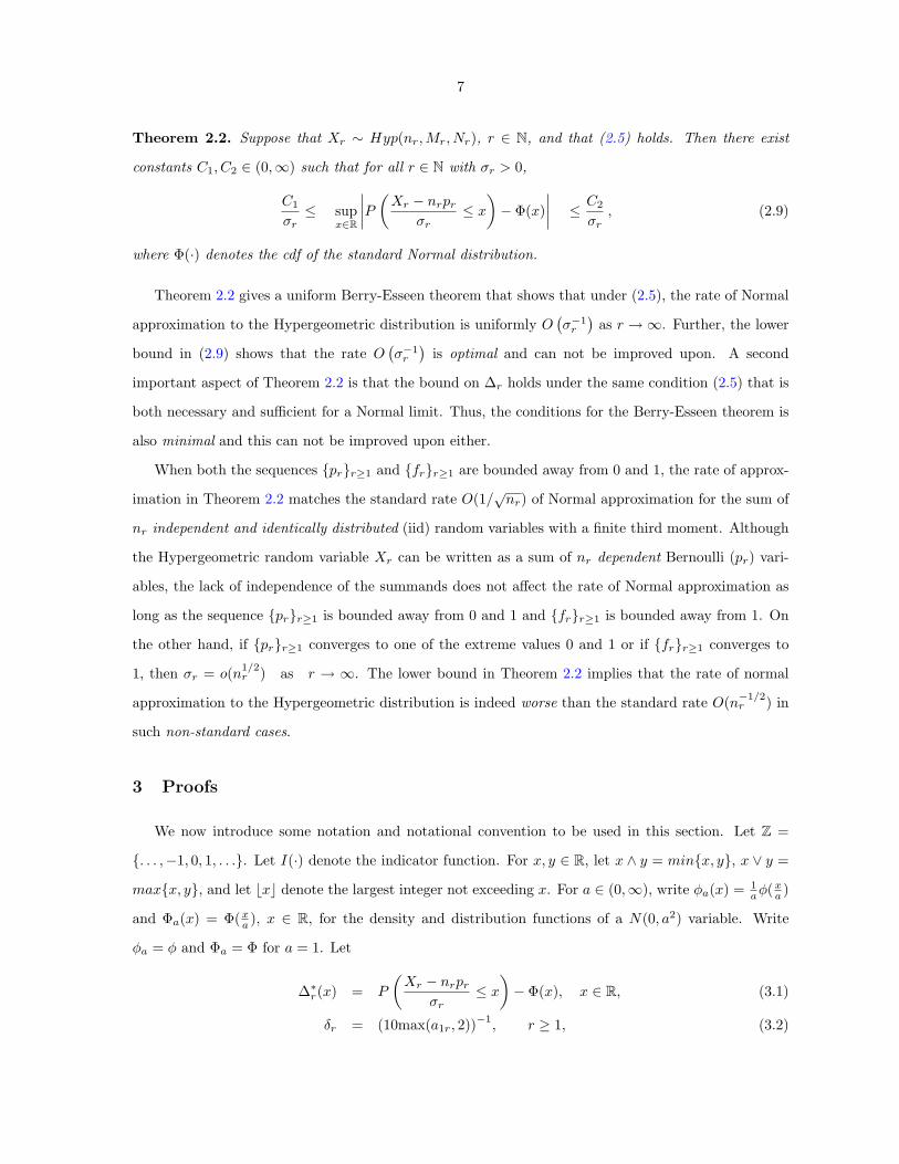
Theorem 2.2. Suppose that Xr ∼ Hyp(nr,Mr, Nr), r ∈ N, and that (2.5) holds. Then there exist
constants C1, C2 ∈ (0,∞) such that for all r ∈ N with σr > 0,
C1
σr≤ sup
x∈R
∣∣∣∣P (Xr − nrpr
σr≤ x
)− Φ(x)
∣∣∣∣ ≤ C2
σr, (2.9)
where Φ(·) denotes the cdf of the standard Normal distribution.
Theorem 2.2 gives a uniform Berry-Esseen theorem that shows that under (2.5), the rate of Normal
approximation to the Hypergeometric distribution is uniformly O(σ−1
r
)as r →∞. Further, the lower
bound in (2.9) shows that the rate O(σ−1
r
)is optimal and can not be improved upon. A second
important aspect of Theorem 2.2 is that the bound on ∆r holds under the same condition (2.5) that is
both necessary and sufficient for a Normal limit. Thus, the conditions for the Berry-Esseen theorem is
also minimal and this can not be improved upon either.
When both the sequences prr≥1 and frr≥1 are bounded away from 0 and 1, the rate of approx-
imation in Theorem 2.2 matches the standard rate O(1/√nr) of Normal approximation for the sum of
nr independent and identically distributed (iid) random variables with a finite third moment. Although
the Hypergeometric random variable Xr can be written as a sum of nr dependent Bernoulli (pr) vari-
ables, the lack of independence of the summands does not affect the rate of Normal approximation as
long as the sequence prr≥1 is bounded away from 0 and 1 and frr≥1 is bounded away from 1. On
the other hand, if prr≥1 converges to one of the extreme values 0 and 1 or if frr≥1 converges to
1, then σr = o(n1/2r ) as r → ∞. The lower bound in Theorem 2.2 implies that the rate of normal
approximation to the Hypergeometric distribution is indeed worse than the standard rate O(n−1/2r ) in
such non-standard cases.
3 Proofs
We now introduce some notation and notational convention to be used in this section. Let Z =
. . . ,−1, 0, 1, . . .. Let I(·) denote the indicator function. For x, y ∈ R, let x ∧ y = minx, y, x ∨ y =
maxx, y, and let bxc denote the largest integer not exceeding x. For a ∈ (0,∞), write φa(x) = 1aφ(x
a )
and Φa(x) = Φ(xa ), x ∈ R, for the density and distribution functions of a N(0, a2) variable. Write
φa = φ and Φa = Φ for a = 1. Let
∆∗r(x) = P
(Xr − nrpr
σr≤ x
)− Φ(x), x ∈ R, (3.1)
δr = (10max(a1r, 2))−1, r ≥ 1, (3.2)

8
where a1r = fr+44(1−fr)
and where fr = fr if fr ≤ 12 and fr = 1− fr if fr >
12 . We shall use C to denote a
generic positive constant that does not depend on r. Unless otherwise stated, limits in order symbols
are taken by letting r →∞.
The first result gives a basic approximation to Hypergeometric probabilities solely under condition
(3.3) stated below.
Lemma 3.1. Suppose that X ∼ Hyp(n;M,N) for a given set of integers n,M,N ∈ N such that
0 < f < 1, 0 < p < 1 and 6(np ∧ nq) ≥ 1, (3.3)
where f = nN , p = M
N and q = 1− p. Then, for any given δ ∈ (0, 12 ],
logP (k;n,M,N) = −x2
k,n
2(1− f)− 1
2log (2πnpq(1− f)) +R∗n(k) (3.4)
for all k ∈ 0, . . . , n, where P (k;n,M,N) = P (X = k) (cf. (1.1)), xk,n = x−np√npq and ak,n =
xk,n
(1−f)√
npq , 0 ≤ k ≤ n and where, for |ak,n| ≤ δ, the remainder term R∗n(k) admits the bound
|R∗n(k)| ≤ 16npq(1− δ)(1− f)
+
[12|ak,n|+ a2
k,n
14
+2δ
(1− δ)3
]
+ |ak,n|3npq(f
4+ 1)
12
+2(1 + δ)(1− δ)3
. (3.5)
The proof of Lemma 3.1 is based on a long and careful analysis of the Hypergeometric probabilities
in (1.1) using Stirling’s approximation. For the proofs of Lemma 3.1 and of the next two results, see
Lahiri et al. (2006).
Lemma 3.2. Let g : R −→ [0,∞) be such that g is ↑ on (−∞, a) and g is ↓ on (a,∞) for some a ∈ R.
Then, for any k ∈ N, b ∈ R and h ∈ (0,∞),
k∑i=o
g(b+ ih) ≤∫ b+hk
b
g(x)dx+ 2hg(x0), (3.6)
where g(x0) = maxg(b+ ih) : i = 0, 1, . . . , k.
Lemma 3.3. Let φ(x) = 1√2π
exp(−x2/2), x ∈ R. Then, for any h ∈ (0,∞), b ∈ [0,∞), j0 ∈ N,
∣∣∣∣h j0∑i=0
φ(b+ ih)−∫ b+(j0+
12 )h
b−h2
φ(x)dx∣∣∣∣ (3.7)
≤ h2
12
[∫ b+j0h+ h2
b−h2
|φ′′(x)|dx+ (4 + h) sup
|φ′′(x)| : −h
2< x− b < j0h+
h
2
].

9
Proof of Theorem 2.1: Suppose that (2.5) holds. Fix ε ∈ (0, 1). By Chebyshev’s inequality, for all
r ∈ N,
P
(∣∣∣∣Xr − nrpr
σr
∣∣∣∣ > 2ε
)≤ ε2
4· Nr
Nr − 1. (3.8)
By Lemmas 3.1 and 3.3, for any r ∈ N with fr ≤ 12 ,
∆1r(ε) ≡ sup− 2
ε≤a<b≤ 2ε
∣∣∣∣P (a < Xr − nrpr
σr≤ b
)− [Φ(b)− Φ(a)]
∣∣∣∣≤
∑− 2σr
ε <k−nrpr≤ 2σrε
∣∣∣∣P (k;nr,Mr, Nr)−1σrφ
(k − nrpr
σr
) ∣∣∣∣+
∑− 2
ε≤a<b≤ 2ε
∣∣∣∣ ∑aσr<k−nrpr≤bσr
1σrφ
(k − nrpr
σr
)− [Φ(b)− Φ(a)]
∣∣∣∣≤ C
σ2r
∑− 2σr
ε <k−nrpr≤ 2σrε
exp(C
σr
)exp
(− (k − nrpr)
2
σ2r
[12− C
σr
])
+C
σ2r
[∫ ∞
−∞|φ′′(x)|dx+ 1
]+
2√2πσr
≤ C
σr
[∫ ∞
−∞exp
(−x
2
4
)dx+ 1
],
provided Cσr< 1
4 . Hence, there exists an r0 ∈ N such that for all r ≥ r0 with fr ≤ 12 , ∆1r(ε) < ε
4 . Also
by Mill’s ratio, Φ(− 2ε ) + 1 − Φ( 2
ε ) < εφ( 2ε ). Hence, using (3.8) and the above inequalities, it can be
shown that for all r ≥ r0 with fr ≤ 12 ,
∆r(ε) < ε. (3.9)
Next suppose that fr >12 . Consider the collection of Nr − nr objects that are left after the sample
of size nr has been selected from the population of size Nr. Let Yr =the number of ‘type A’-objects in
this collection. Then,
Yr ∼ Hyp(Nr − nr;Mr, Nr) and P (Xr = j) = P (Yr = Mr − j), (3.10)
for all r ∈ N and j ∈ Z. Hence, V ar(Yr) = V ar(Xr), and P (Xr ≤ k) = P (Yr ≥ Mr − k). Thus, for
each x ∈ R,
P
(Xr − nrpr
σr≤ x
)= P (Xr ≤ bnrpr + xσrc)
= P (Yr ≥Mr − bnrpr + xσrc)
= P
(Yr − (Nr − nr)pr
σr≥ Mr − bnrpr + xσrc − (Nr − nr)pr
σr
)= P (Yr ≥ xr) (say),
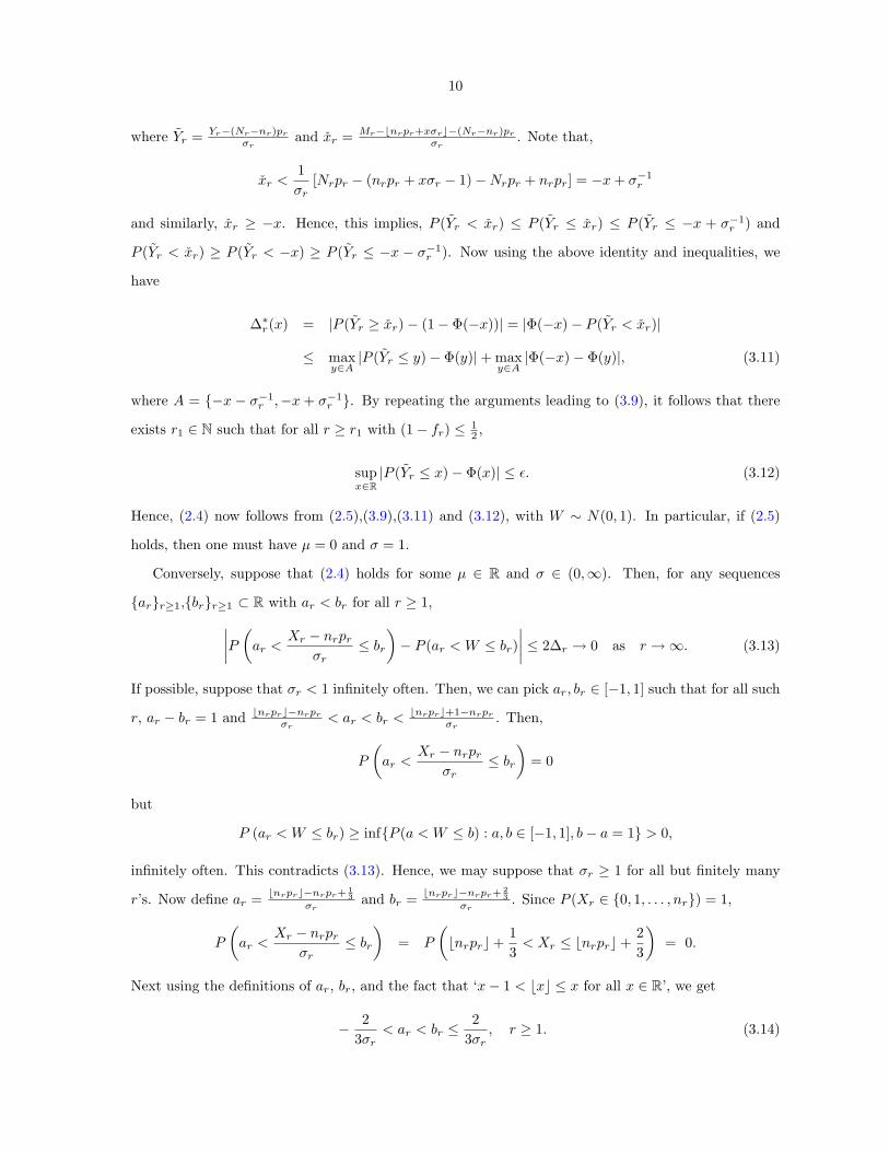
10
where Yr = Yr−(Nr−nr)pr
σrand xr = Mr−bnrpr+xσrc−(Nr−nr)pr
σr. Note that,
xr <1σr
[Nrpr − (nrpr + xσr − 1)−Nrpr + nrpr] = −x+ σ−1r
and similarly, xr ≥ −x. Hence, this implies, P (Yr < xr) ≤ P (Yr ≤ xr) ≤ P (Yr ≤ −x + σ−1r ) and
P (Yr < xr) ≥ P (Yr < −x) ≥ P (Yr ≤ −x − σ−1r ). Now using the above identity and inequalities, we
have
∆∗r(x) = |P (Yr ≥ xr)− (1− Φ(−x))| = |Φ(−x)− P (Yr < xr)|
≤ maxy∈A
|P (Yr ≤ y)− Φ(y)|+ maxy∈A
|Φ(−x)− Φ(y)|, (3.11)
where A = −x − σ−1r ,−x + σ−1
r . By repeating the arguments leading to (3.9), it follows that there
exists r1 ∈ N such that for all r ≥ r1 with (1− fr) ≤ 12 ,
supx∈R
|P (Yr ≤ x)− Φ(x)| ≤ ε. (3.12)
Hence, (2.4) now follows from (2.5),(3.9),(3.11) and (3.12), with W ∼ N(0, 1). In particular, if (2.5)
holds, then one must have µ = 0 and σ = 1.
Conversely, suppose that (2.4) holds for some µ ∈ R and σ ∈ (0,∞). Then, for any sequences
arr≥1,brr≥1 ⊂ R with ar < br for all r ≥ 1,∣∣∣∣P (ar <Xr − nrpr
σr≤ br
)− P (ar < W ≤ br)
∣∣∣∣ ≤ 2∆r → 0 as r →∞. (3.13)
If possible, suppose that σr < 1 infinitely often. Then, we can pick ar, br ∈ [−1, 1] such that for all such
r, ar − br = 1 and bnrprc−nrpr
σr< ar < br <
bnrprc+1−nrpr
σr. Then,
P
(ar <
Xr − nrpr
σr≤ br
)= 0
but
P (ar < W ≤ br) ≥ infP (a < W ≤ b) : a, b ∈ [−1, 1], b− a = 1 > 0,
infinitely often. This contradicts (3.13). Hence, we may suppose that σr ≥ 1 for all but finitely many
r’s. Now define ar = bnrprc−nrpr+ 13
σrand br = bnrprc−nrpr+ 2
3σr
. Since P (Xr ∈ 0, 1, . . . , nr) = 1,
P
(ar <
Xr − nrpr
σr≤ br
)= P
(bnrprc+
13< Xr ≤ bnrprc+
23
)= 0.
Next using the definitions of ar, br, and the fact that ‘x− 1 < bxc ≤ x for all x ∈ R’, we get
− 23σr
< ar < br ≤2
3σr, r ≥ 1. (3.14)

11
By (3.13) and (3.14), it follows that
13σr
minφσ(x− µ) : |x| ≤ 23σr
≤∫ br
ar
φσ(x− µ)dx = P (ar < W ≤ br)
=∣∣∣P (ar <
Xr − nrpr
σr≤ br
)− P (ar < W ≤ br)
∣∣∣→ 0 as r →∞.
As a result, σr →∞ as r →∞ and (2.5) holds. This completes the proof of the theorem.
Proof of Theorem 2.2: Let r ∈ N be an integer such that σrδr > 1. First, suppose that fr ≤ 12 .
Consider the case x ≤ 0. For k = 0, 1, . . . , nr, let xk ≡ xk,r = k−npσ , and define
K0,r = supk ∈ Z+ : xk ≤ 0, K1,r = infk ∈ Z+ : xk ≥ −1
K2,r = infk ∈ Z+ : xk ≥ −δrσr and Jx,r = bnp+ xσc, x ∈ R,
where δr ∈ (0, 12 ] is as in (3.2). For notational simplicity, we drop the subscript r from the indices
xk,r,K0,r,K1,r,K2,r and Jx,r. Note that by definition, K1−1 < nrpr−σr ≤ K1, K2−1 < nrpr−δrσ2r ≤
K2, xj,r ∈ [−1, 0] for all K1 ≤ j ≤ K0 and xj,r ∈ [−δrσr,−1) for all K2 ≤ j < K1. Hence, for any
x ∈ [−δrσr, 0],
|∆∗r(x)| ≤ P (Xr < K2) +
Jx∑j=K2
∣∣∣∣P (Xr = j)− φ(xj,r)σr
∣∣∣∣+ ∣∣∣∣ Jx∑j=K2
φ(xj,r)σr
− Φ(x)∣∣∣∣
= I1,r + I2,r(x) + I3,r(x), say. (3.15)
By Chebyshev’s inequality, noting that K2 − 1 < nrpr − δrσ2r ≤ K2, we have
I1,r ≡ P (Xr ≤ K2 − 1) ≤ P
(∣∣∣∣Xr − nrpr
σr
∣∣∣∣ ≥ ∣∣∣∣K2 − nrpr − 1σr
∣∣∣∣)≤ V ar(Xr)
(K2 − 1− nrpr)2 ≤
Nrσ2r
Nr − 1(δrσ2
r)−2
≤ 2δ2rσ
2r
. (3.16)
Next, consider I2,r(x) for x ∈ [−δrσr,−1). Note that for x < −1, Jx−nrpr
σr≤ x < −1. Hence
Jx < K1 and xj,r < −1 for all j < Jx. From Lemma 3.1, writing R∗r(j) ≡ R∗nr(j), we get
|R∗r(j)| ≤1
6σ2r(1− δr)
+
[|xj,r|2
2σr+|xj,r|2
σ2r
14
+2δr
(1− δr)3
+|xj,r|3
2σrAr
](3.17)

12
for all K2 ≤ j < K1, where Ar = a1,r
(1 + 4(1+δr)
(1−δr)3
)and a1,r = fr+4
4(1−fr) . It is easy to verify that δr ≤ 120
and δrAr < .59 for all r satisfying δrσr > 1. Hence
|R∗r(j)| ≤ (0.2)σ−2r +
x2j,r
2
[1σr
+2σ2
r
(0.3667) + δrAr
]≤ (0.2)σ−2
r +x2
j,r
2
[min0.86,
65σr
+ 0.59]. (3.18)
Now, from (3.17), for all K2 ≤ j < K1,
|R∗r(j)| ≤ (0.2)σ−2r + |xj,r|3
∣∣∣∣ [ 12σr
+1σ2
r
(0.3667) +3a1,r
σr
]≤ 4|xj,r|3
a1,r
σr. (3.19)
Next note that for any a ∈ (0,∞), the function g(y; a) = y3 exp(−ay), y ∈ [0,∞), is increasing on
[0,√
3/2a], and decreasing on (√
3/2a,∞). Hence, by Lemmas 3.1 and 3.2, (3.18) and (3.19), with
c = .07, we have
I2,r(x) ≤Jx∑
j=K2
∣∣∣∣φ(xj,r)σr
exp(R∗r(j))−φ(xj,r)σr
∣∣∣∣≤ 1
σr
Jx∑j=K2
φ(xj,r)|R∗r(j)| exp(|R∗r(j)|)
≤ 4a1,r√2πσ2
r
exp(σ−2r )
Jx∑j=K2
|xj,r|3 exp(−cx2j,r) ≤
C
σr. (3.20)
Also, noting that |R∗r(j)| ≤ 1σr
+[(.43)x2
j,r
]∧ 4a1,r
σrfor all K1 ≤ j ≤ K0 and K0 −K1 ≤ σr, by Lemma
3.1, it follows that
K0∑j=K1
∣∣∣∣P (X = j)− 1σrφ(xj,r)
∣∣∣∣ ≤ K0∑j=K1
exp
(−x2
j,r
2
)|R∗r(j)|
exp(|R∗r(j)|)√2πσr
.
≤ (K0 −K1) exp(σ−1r )
5a1,r√2πσ2
r
≤ C
σr. (3.21)
Thus, the bound (3.20) on I2,r(x) holds for all x ∈ [−δrσr, 0]. Next note that by definition, xJx,r ≤ x
and xK2,r ≤ −δrσr + σ−1r . Hence, for x ∈ [−δrσr, 0], by Lemma 3.3,
I3,r(x) ≤∣∣∣∣ 1σr
Jx∑j=K2
φ(xj,r)−∫ xJx,r+(2σr)−1
xK2,r−(2σr)−1φ(y)dy
∣∣∣∣+∣∣∣∣Φ(x)− Φ
(xJx,r +
1(2σr)
) ∣∣∣∣+ Φ(xK2,r −
1(2σr)
)
≤ 112σ2
r
[∫ x+ 12σr
−∞|φ′′(y)|dy + 5 max|φ
′′(y)| : −∞ < y < x+
12σr
]
+ Φ(x+
12σr
)− Φ
(x− 1
2σr
)+ Φ(−δrσr +
12σr
)
≤ C
σr. (3.22)
13
Since sup−∞≤x≤−δrσr|∆∗
r(x)| ≤ P (Xr ≤ K2 − 1) + Φ(−δrσr) ≤ Cδ2
rσ2r,
supx∈(−∞,0]
|∆∗r(x)| ≤ C/σr for fr ≤ 1/2. (3.23)
To establish the upper bound for x ≥ 0 and fr ≤ 12 , define Vr = nr − Xr, r ∈ N. Note that
Vr has a Hypergeometric distribution with parameters nr, Nr −Mr, Nr. Further, [Xr − nrpr]/σr =
−[Vr − nrqr]/σr for all r ∈ N. Hence, the desired upper bound on the right tails of [Xr − nrpr]/σr,
can be obtained by repeating the arguments above with Xr replaced by Vr and pr replaced by qr for
any r such that δrσr > 1. This, together with (3.23) proves the upper bound in Theorem 2.2 for all
r satisfying fr ≤ 12 and δrfr > 1. The proof of the upper bound in (2.9) for ‘fr ∈ [ 12 , 1) and x ∈ R’
follows by replacing the above arguments with Xr, fr replaced by Yr, 1 − fr respectively and using
the bound (3.10) and (3.11). To establish the lower bound in (2.9), write x∗r = (bnrprc − nrpr)/σr.
Clearly, lim infr→∞ σr∆r ≥ lim infr→∞ σr
∣∣∣∆∗r(x
∗r)∣∣∣ ≡ C0, say. If C0 > 0, then ∆r >
C02σr
for all but
finitely many r’s and the lower bound holds. On the other hand, if C0 = 0, then using the fact that
σ−1r (Xr − nrpr) is a lattice random variable with maximal span σ−1
r , we get
lim infr→∞
σr∆r ≥ lim infr→∞
σr
∣∣∣∆∗r(x
∗r + [2σr]−1)
∣∣∣= lim inf
r→∞σr
∣∣∣∆∗r(x
∗r) + Φ(x∗r)− Φ(x∗r + [2σr]−1)
∣∣∣ = φ(0)/2 > 0.
This completes the proof of Theorem 2.2.
14
NORMAL APPROXIMATION TO THE HYPERGEOMETRIC
DISTRIBUTION IN NONSTANDARD CASES AND A SUB-GAUSSIAN
BERRY-ESSEEN THEOREM
A paper accepted in the Journal of Statistical Planning and Inference1
Soumendra N. Lahiri, Arindam Chatterjee and Tapabrata Maiti
Abstract
In this paper, we consider simple random sampling without replacement from a dichotomous finite
population. We investigate accuracy of the Normal approximation to the Hypergeometric probabilities
for a wide range of parameter values, including the nonstandard cases where the sampling fraction tends
to one and where the proportion of the objects of interest in the population tends to the boundary values,
zero and one. We establish a non-uniform Berry-Esseen theorem for the Hypergeometric distribution
which shows that in the nonstandard cases, the rate of Normal approximation to the Hypergeometric
distribution can be considerably slower than the rate of Normal approximation to the Binomial distri-
bution. We also report results from a moderately large numerical study and provide some guidelines
for using the Normal approximation to the Hypergeometric distribution in finite samples.
1 Introduction
Consider a dichotomous finite population of sizeN havingM objects of ‘type A’ andN−M objects of
‘type B’. Suppose a sample of size n is drawn at random, without replacement from this population. Let
X denote the number of ‘type A’-individuals in the sample. Then, X is said to have the Hypergeometric
distribution with parameters n,M,N , written as X ∼ Hyp(n;M,N). The probability mass function
1available at http://dx.doi.org/10.1016/j.jspi.2007.03.033

15
(p.m.f) of X is given by,
P (X = x) ≡ P (x;n,M,N) =
(M
x )(N−Mn−x )
(Nn) if x = 0, 1 . . . , n
0 otherwise,(1.1)
where, for any two integers r ≥ 1 and s,
(r
s
)=
r!
s!(r−s)! if 0 ≤ s ≤ r
0 otherwise,(1.2)
with 0! = 1 and r! = 1 · 2 · · · r. Let f = nN denote the sampling fraction and let p = M
N denote the pro-
portion of the ‘type A’-objects in the population. The Hypergeoemetric distribution plays an important
role in many areas of statistics, including sample surveys (Burstein (1975) and Wendell and Schmee
(1996)), capture-recapture methods (Seber (1970) and Wittes (1972)), analysis of contingency tables
(Blyth and Staudte (1997)), statistical quality control (von Collani (1986), Patel and Samaranayake
(1991) and Sohn (1997)), etc. Normal approximations to the Hypergeometric probabilities P (.;n,M,N)
of (1.1) are classical in the cases where the sampling fraction f and the proportion p are bounded away
from 0 and 1; for example, see Feller (1971). The nonstandard cases correspond to the extremes where
f or p take values near the boundary values 0 and 1. Although the nonstandard cases arise frequently in
all these areas of applications, the validity and accuracy of the Normal approximation in such situations
are not well studied. The quality of Normal approximation deteriorates as the parameters f and p tend
to their boundary values. For example, consider the following table where the cumulative distribution
function (cdf) of the centered and scaled version X−E(X)√V ar(X)
of X at zero is approximated by the Normal
cdf at zero for different values of f and p.
Table 1 Values of ∆(N, p, f) (cf. 3.1) at x = 0 for various p and f . Here,N = 200 and M = Np and n = Nf .
p f = 0.5 f = 0.6 f = 0.7 f = 0.8 f = 0.90.5 0.0562 0.0574 0.0613 0.0701 0.09290.6 0.0574 0.0593 0.0641 0.0743 0.09950.7 0.0613 0.0641 0.0702 0.0822 0.11120.8 0.0701 0.0743 0.0822 0.0972 0.13210.9 0.0929 0.0995 0.1112 0.1321 0.1787
Table 1 gives the values of the absolute difference of the cdfs of X−E(X)√V ar(X)
and the standard Normal
distribution at x = 0. The population size is fixed at N = 200 while the proportion p of ‘Type A’-objects
16
and the sampling fraction f are varied over a range of 0.5 to 0.9 in increments of 0.1 (The values of
p and f between 0 and 0.5 are omitted due to the symmetry of the problem). In particular, for these
choices of N and f , the sample size n = Nf takes the values 100, 120, 140, 160 and 180. Note that even
for such moderately large sample sizes, the error of approximation increases steadily as p approaches
the boundary value 1. Indeed, for p = .9 and f = .9, the error of approximation is as high as 0.179
at the origin in the finite population sampling framework, which is significantly higher than 0.036, the
error of Normal approximation to the Binomial cdf with parameters n = 180 and p = .9. This shows
that the commonly known approximation results for the ‘with replacement sampling’ (or sampling from
an infinite population) case do not give a representative picture in the finite population setting when
the parameters p and f are close to their boundary values. For a better understanding, one needs to
be able to quantify the accuracy of Normal approximation as a function of N , p and f in the finite
population setting.
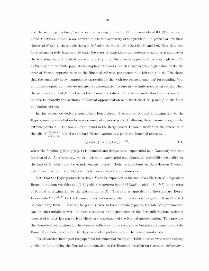
In this paper, we derive a nonuniform Berry-Esseen Theorem on Normal approximation to the
Hypergeometric distribution for a wide range of values of p and f , allowing these parameters go to the
extreme points 0, 1. The non-uniform bound in the Berry-Esseen Theorem shows that the difference of
the cdfs of X−E(X)√V ar(X)
and of a standard Normal variate at a point x is bounded above by
g(x)[Nf(1− f)p(1− p)]−1/2, (1.3)
where the function g(x) = g(x; p, f) is bounded and decays at an exponential (sub-Gaussian) rate as a
function of x. As a corollary, we also derive an exponential (sub-Gaussian) probability inequality for
the tails of X, which may be of independent interest. Both the sub-Gaussian Berry-Esseen Theorem
and the exponential inequality seem to be new even in the standard case.
Note that the Hypergeometric variable X can be expressed as the sum of a collection of n dependent
Bernoulli random variables and (1.3) yields the uniform bound O([np(1− p)(1− f)]−1/2
)on the error
of Normal approximation to the distribution of X. This rate is equivalent to the standard Berry-
Esseen rate O(n−1/2
)for the Binomial distribution only when p is bounded away from 0 and 1 and f
bounded away from 1. However, for p and f close to these boundary points, the rate of approximation
can be substantially slower. In such situations, the dependence of the Bernoulli random variables
associated with X has a nontrivial effect on the accuracy of the Normal approximation. This provides
the theoretical justification for the observed difference in the accuracy of Normal approximations to the
Binomial probabilities and to the Hypergeometric probabilities in the nonstandard cases.
The theoretical findings of the paper and the numerical example in Table 1 also show that the existing
guidelines for applying the Normal approximation to the Binomial distribution (based on independent

17
Bernoulli random variables) are not appropriate for the Hypergeometric distribution in the nonstandard
cases. To formulate a working guideline in such situations, we conduct a moderately large numerical
study and investigate the effect of the dependence in finite samples. On the basis of the numerical study,
in Section 3, we provide some ’quick and easy’ guidelines for assessing the error of Normal approximation
to the Hypergeometric distribution in practice.
The rest of the paper is organized as follows. We conclude Section 1 with a brief literature review.
Section 2 introduces the asymptotic framework and states the Berry-Esseen theorem and the exponential
inequality. Results from the numerical study are reported in Section 3. Proofs of all the results are
given in Section 4.
For results on Normal approximations to Hypergeometric probabilities in the standard case where the
sampling fraction f and the proportion p are bounded away from 0 and 1, see Feller (1971). For general
p and f , Nicholson (1956) derived some very precise bounds for the point probabilities P (.;n,M,N) (cf.
(1.1)) using some special normalizations of the Hypergeometric random variable X. General methods
for proving the central limit theorem (CLT) for sample means under sampling without replacement
from finite populations are given by Madow (1948)), Erdos and Renyi (1959) and Hajek (1960). In
relation to the earlier work, the main contribution of our paper is to establish a non-uniform Berry-
Esseen Theorem for the Hypergeometric distribution for a wide range of parameter values, including
the nonstandard case, and to provide some practical guidelines for using the Normal approximation in
finite sample applications.
2 Main Results
Let r be a positive integer valued variable and for each r ∈ N (where N = 1, 2, . . .), let Xr be a
random variable having the Hypergeometric distribution of (1.1) with parameters (nr,Mr, Nr), where
nr,Mr, Nr ∈ N. Thus we consider a sequence of dichotomous finite populations indexed by r, with the
population of objects of type A and the sampling fraction respectively given by,
pr =Mr
Nrand fr =
nr
Nr∀r ∈ N. (2.1)
Let
σ2r ≡ Nrprqrfr(1− fr), (2.2)
where qr = 1−pr. Also, let φ(·) and Φ(·) respectively denote the density and the distribution function of
a standard Normal random variable, i.e., φ(x) = 1√2π
exp(−x2
2 ), x ∈ R and Φ(x) =∫ x
−∞ φ(t)dt, x ∈

18
R. Let I(·) denote the indicator function. For x, y ∈ R, write x ∧ y = minx, y. Define
δr =110
(max(a1r, 2))−1, r ≥ 1, (2.3)
where a1r = fr+44(1−fr)
and where fr = minfr, 1− fr. Then, we have the following result.
Theorem 2.1. Suppose that Xr ∼ Hyp(nr,Mr, Nr), r ∈ N. Assume that r is such that
δrσr > 1. (2.4)
Then there exists universal constants C1, C2 ∈ (0,∞) (not depending on r, nr,Mr and Nr) such that∣∣∣∣P (Xr − nrpr
σr≤ x
)− Φ(x)
∣∣∣∣ ≤ C1
σr
1 + |x|2
λr(x)exp
(−C2x
2λ2r(x)
)(2.5)
for all x ∈ R, where λr(x) = qrI(x ≤ 0) + prI(x ≥ 0).
Theorem 2.1 is a non-uniform Berry-Esseen Theorem for the Hypergeometric distribution. It shows
that the error of Normal approximation to the Hypergeometric distribution dies at a sub-Gaussian rate
in the tails. The only condition needed for the validity of this bound is (2.4). It is easy to check that
δr ∈(
125,
120
](2.6)
for all r satisfying (2.4). Hence, the bound in (2.5) is available for all r such that σr ≥ 25.
As pointed out in Section 1, when both the sequences prr≥1 and frr≥1 are bounded away
from 0 and 1, the rate of approximation in Theorem 2.1 matches the standard rate O(n− 1
2r
)of Normal
approximation for the sum of nr iid random variables with a finite third moment. Although the
Hypergeometric random variable Xr can be written as a sum of nr dependent Bernoulli (pr) variables,
the lack of independence of the summands does not affect the rate of Normal approximation as long
as the sequence prr≥1 is bounded away from 0 and 1 and frr≥1 is bounded away from 1. On the
other hand, if either of the sequences prr≥1 and frr≥1 converge to one of the extreme values 0
and 1, then
σr = o(n
12r
)as r →∞
and the rate of Normal approximation to the Hypergeometric distribution is indeed worse than the
standard rate O(n− 1
2r
)in such non-standard cases. An immediate consequence of Theorem 2.1 is the
following exponential (sub-Gaussian) probability bound on the tails of Xr.

19
Theorem 2.2. Suppose that Xr ∼ Hyp(nr,Mr, Nr), r ∈ N. Then, there exist universal constants
C3, C4 ∈ (0,∞) (not depending on r, nr,Mr, Nr) such that for all r satisfying (2.4),
P
(∣∣∣∣Xr − nrpr
σr
∣∣∣∣ ≥ x
)≤ C3
(pr ∧ qr)3exp
(−C4x
2[pr ∧ qr]2)
for all x > 0. (2.7)
3 Numerical results
To gain some insight into the quality of Normal approximation to the Hypergeometric distribution
in finite samples and to compare it with the accuracy in the case of the Binomial distribution, first
we consider some joint plots of the cdfs of normalized Hypergeometric and Binomial random variables
against the standard Normal cdf. Figures 1-5 show these plots for different values of the parameters n
and p for N = 60, 200.
From the figures, it follows that the quality of Normal approximation to the Hypergeometric distri-
bution is comparable to that for the Binomial distribution for values of f and p close to .5, but there
is a stark loss of accuracy for high values of f and p.
Next, to get a quantitative picture of the error of Normal approximation, we conducted a moderately
large numerical study with different values of the population size N and with different values of the
parameters p and f . The population sizes considered were N = 60, 200, 500, 2000. For a given value of
N , the set of values of p and f considered was 0.5, 0.6, 0.7, 0.8, 0.9. We considered the Kolmogorov
distance, i.e., the maximal distance between the cdfs of the normalized Hypergeometric variable and a
standard Normal variable as a measure of accuracy. More specifically, the measure of accuracy for the
Hypergeometric case is defined as
∆(N, p, f) =∣∣∣∣P (X − np
σ≤ x
)− Φ(x)
∣∣∣∣ , (3.1)
where X ∼ Hyp(n,M,N), f = n/N , p = M/N , σ2 = Nf(1 − f)p(1 − p) and Φ(·) denotes the cdf of
the N(0, 1) distribution.
Tables 2-5 give the values of ∆(N, p, f) for different combinations of the parameter values as indicated
above. For comparison, we also included the values of the maximal distance of the cdfs of normalized
Binomial (n, p) and N(0,1) random variables.
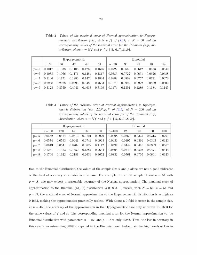
From Tables 2-5, it follows that the accuracy of the Normal approximation to the Hypergeometric
distribution deteriorates as p or f tend to the boundary value 1. Unlike the case of Normal approxima-
20
Table 2 Values of the maximal error of Normal approximation to Hyperge-ometric distribution (viz., ∆(N, p, f) of (3.1)) at N = 60 and thecorresponding values of the maximal error for the Binomial (n,p) dis-tribution where n = Nf and p, f ∈ .5, .6, .7, .8, .9.
Hypergeometric Binomialn=30 36 42 48 54 n=30 36 42 48 54
p=.5 0.1017 0.1038 0.1106 0.1260 0.1646 0.0722 0.0660 0.0612 0.0573 0.0540p=.6 0.1038 0.1066 0.1171 0.1284 0.1817 0.0785 0.0722 0.0661 0.0626 0.0588p=.7 0.1106 0.1171 0.1283 0.1476 0.1844 0.0888 0.0808 0.0757 0.0711 0.0670p=.8 0.2268 0.2528 0.2896 0.3480 0.4633 0.1070 0.0992 0.0922 0.0859 0.0803p=.9 0.3128 0.3550 0.4046 0.4633 0.7169 0.1474 0.1391 0.1289 0.1184 0.1145
Table 3 Values of the maximal error of Normal approximation to Hypergeo-metric distribution (viz., ∆(N, p, f) of (3.1)) at N = 200 and thecorresponding values of the maximal error for of the Binomial (n,p)distribution where n = Nf and p, f ∈ .5, .6, .7, .8, .9.
Hypergeometric Binomialn=100 120 140 160 180 n=100 120 140 160 180
p=.5 0.0562 0.0574 0.0613 0.0701 0.0929 0.0398 0.0363 0.0337 0.0315 0.0297p=.6 0.0574 0.0593 0.0641 0.0743 0.0995 0.0433 0.0395 0.0366 0.0343 0.0323p=.7 0.0613 0.0641 0.0702 0.0822 0.1112 0.0491 0.0449 0.0416 0.0389 0.0367p=.8 0.1261 0.1373 0.1559 0.1887 0.2634 0.0595 0.0543 0.0503 0.0471 0.0444p=.9 0.1764 0.1922 0.2181 0.2634 0.3652 0.0832 0.0761 0.0705 0.0661 0.0623
tion to the Binomial distribution, the values of the sample size n and p alone are not a good indicator
of the level of accuracy attainable in this case. For example, for an iid sample of size n = 54 with
p = .8, one may expect a reasonable accuracy of the Normal approximation; The maximal error of
approximation to the Binomial (54, .8) distribution is 0.0803. However, with N = 60, n = 54 and
p = .9, the maximal error of Normal approximation to the Hypergeometric distribution is as high as
0.4633, making the approximation practically useless. With about a 9-fold increase in the sample size,
at n = 450, the accuracy of the approximation in the Hypergeometric case only improves to .1683 for
the same values of f and p. The corresponding maximal error for the Normal approximation to the
Binomial distribution with parameters n = 450 and p = .8 is only .0282. Thus, the loss in accuracy in
this case is an astounding 600% compared to the Binomial case. Indeed, similar high levels of loss in

21
Table 4 Values of the maximal error of Normal approximation to Hypergeo-metric distribution (viz., ∆(N, p, f) of (3.1)) at N = 500 and thecorresponding values of the maximal error for the Binomial (n,p) dis-tribution where n = Nf and p, f ∈ .5, .6, .7, .8, .9.
Hypergeometric Binomialn=250 300 350 400 450 n=250 300 350 400 450
p=.5 0.0356 0.0364 0.0389 0.0445 0.0592 0.0252 0.0230 0.0213 0.0199 0.0188p=.6 0.0364 0.0376 0.0407 0.0472 0.0635 0.0274 0.0250 0.0232 0.0217 0.0205p=.7 0.0389 0.0407 0.0446 0.0523 0.0712 0.0311 0.0284 0.0263 0.0246 0.0232p=.8 0.0801 0.0872 0.0990 0.1200 0.1683 0.0378 0.0345 0.0319 0.0299 0.0282p=.9 0.1124 0.1224 0.1390 0.1683 0.2355 0.0530 0.0484 0.0449 0.0420 0.0396
Table 5 Values of the maximal error of Normal approximation to Hypergeo-metric distribution (viz., ∆(N, p, f) of (3.1)) at N = 2000 and thecorresponding values of the maximal error for the Binomial (n,p) dis-tribution where n = Nf and p, f ∈ .5, .6, .7, .8, .9.
Hypergeometric Binomialn=1000 1200 1400 1600 1800 n=1000 1200 1400 1600 1800
p=.5 0.0178 0.0182 0.0195 0.0223 0.0297 0.0126 0.0115 0.0107 0.0010 0.0094p=.6 0.0182 0.0188 0.0204 0.0237 0.0319 0.0137 0.0125 0.0116 0.0109 0.0102p=.7 0.0195 0.0204 0.0224 0.0263 0.0358 0.0156 0.0142 0.0132 0.0123 0.0116p=.8 0.0401 0.0437 0.0496 0.0602 0.0846 0.0189 0.0173 0.0160 0.0150 0.0141p=.9 0.0564 0.0614 0.0698 0.0846 0.1189 0.0266 0.0243 0.0225 0.0210 0.0198
accuracy occur for values of f and p near 1 even when the population size N is increased to 2000 and
beyond. As a consequence, the commonly used guidelines for the accuracy in the Binomial case can be
misleading for assessing accuracy of the Normal approximation to the Hypergeometric distribution in
the extreme cases.
From Tables 2-5, it also follows that for a given value of N , if the parameter p is held fixed at a given
level, the maximal error of approximation to the Hypergeometric distribution increases monotonically
as the value of f (i.e., n) increases, and vice versa. However, the sample size n and the value of p
alone do not give a true indication of the accuracy of the Normal approximation to the Hypergeometric
distribution. To get a better estimate of the level of accuracy, one must consider the combined effect of
all three parameters N , f and p. Theorem 2.1 implies that the combined effect of all three parameters
22
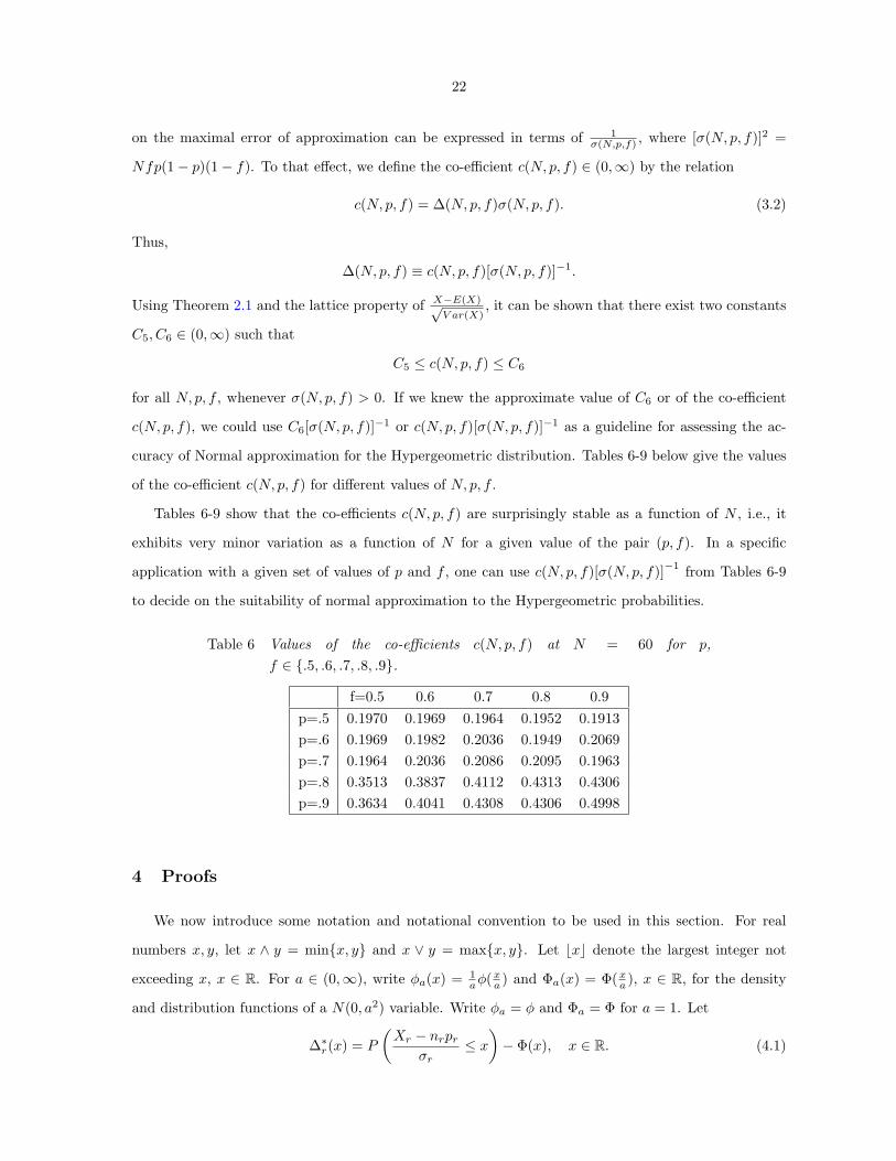
on the maximal error of approximation can be expressed in terms of 1σ(N,p,f) , where [σ(N, p, f)]2 =
Nfp(1− p)(1− f). To that effect, we define the co-efficient c(N, p, f) ∈ (0,∞) by the relation
c(N, p, f) = ∆(N, p, f)σ(N, p, f). (3.2)
Thus,
∆(N, p, f) ≡ c(N, p, f)[σ(N, p, f)]−1.
Using Theorem 2.1 and the lattice property of X−E(X)√V ar(X)
, it can be shown that there exist two constants
C5, C6 ∈ (0,∞) such that
C5 ≤ c(N, p, f) ≤ C6
for all N, p, f , whenever σ(N, p, f) > 0. If we knew the approximate value of C6 or of the co-efficient
c(N, p, f), we could use C6[σ(N, p, f)]−1 or c(N, p, f)[σ(N, p, f)]−1 as a guideline for assessing the ac-
curacy of Normal approximation for the Hypergeometric distribution. Tables 6-9 below give the values
of the co-efficient c(N, p, f) for different values of N, p, f .
Tables 6-9 show that the co-efficients c(N, p, f) are surprisingly stable as a function of N , i.e., it
exhibits very minor variation as a function of N for a given value of the pair (p, f). In a specific
application with a given set of values of p and f , one can use c(N, p, f)[σ(N, p, f)]−1 from Tables 6-9
to decide on the suitability of normal approximation to the Hypergeometric probabilities.
Table 6 Values of the co-efficients c(N, p, f) at N = 60 for p,f ∈ .5, .6, .7, .8, .9.
f=0.5 0.6 0.7 0.8 0.9p=.5 0.1970 0.1969 0.1964 0.1952 0.1913p=.6 0.1969 0.1982 0.2036 0.1949 0.2069p=.7 0.1964 0.2036 0.2086 0.2095 0.1963p=.8 0.3513 0.3837 0.4112 0.4313 0.4306p=.9 0.3634 0.4041 0.4308 0.4306 0.4998
4 Proofs
We now introduce some notation and notational convention to be used in this section. For real
numbers x, y, let x ∧ y = minx, y and x ∨ y = maxx, y. Let bxc denote the largest integer not
exceeding x, x ∈ R. For a ∈ (0,∞), write φa(x) = 1aφ(x
a ) and Φa(x) = Φ(xa ), x ∈ R, for the density
and distribution functions of a N(0, a2) variable. Write φa = φ and Φa = Φ for a = 1. Let
∆∗r(x) = P
(Xr − nrpr
σr≤ x
)− Φ(x), x ∈ R. (4.1)
23
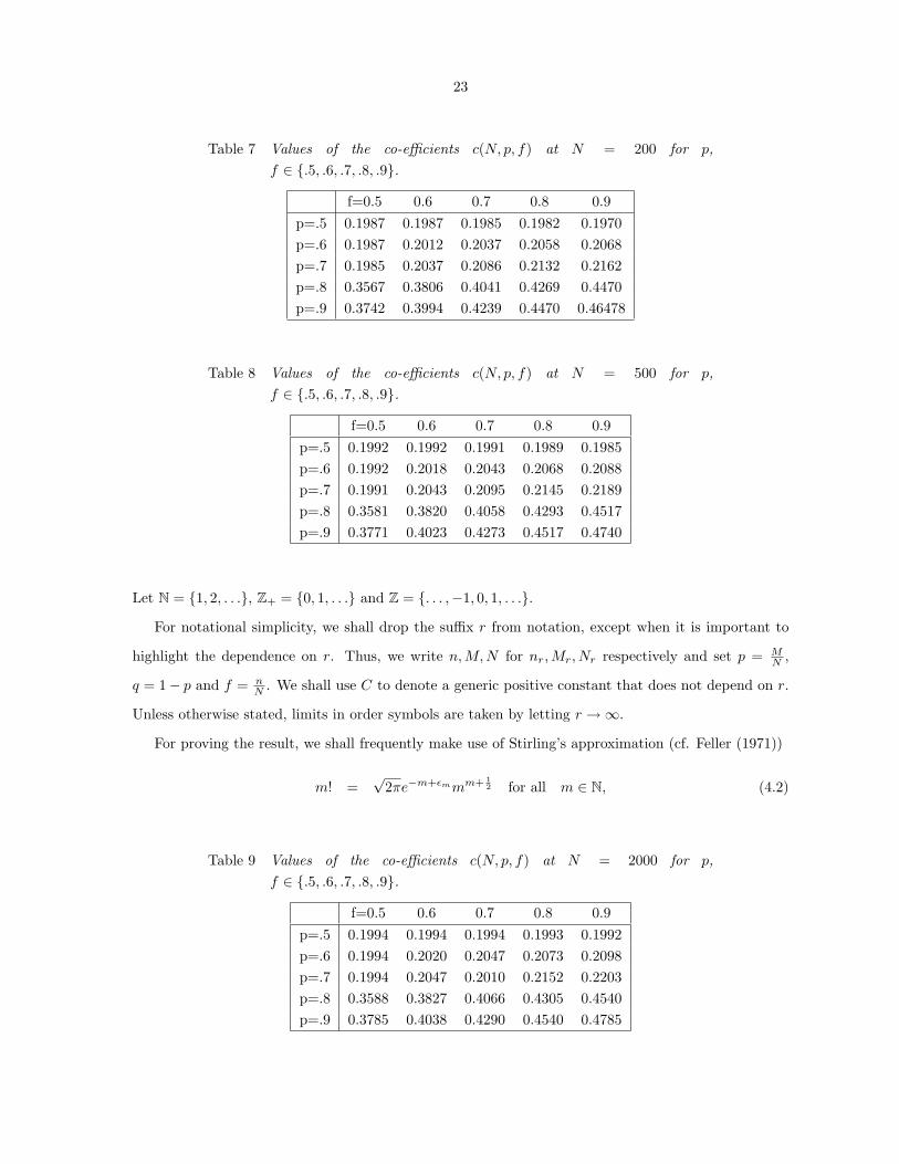
Table 7 Values of the co-efficients c(N, p, f) at N = 200 for p,f ∈ .5, .6, .7, .8, .9.
f=0.5 0.6 0.7 0.8 0.9p=.5 0.1987 0.1987 0.1985 0.1982 0.1970p=.6 0.1987 0.2012 0.2037 0.2058 0.2068p=.7 0.1985 0.2037 0.2086 0.2132 0.2162p=.8 0.3567 0.3806 0.4041 0.4269 0.4470p=.9 0.3742 0.3994 0.4239 0.4470 0.46478
Table 8 Values of the co-efficients c(N, p, f) at N = 500 for p,f ∈ .5, .6, .7, .8, .9.
f=0.5 0.6 0.7 0.8 0.9p=.5 0.1992 0.1992 0.1991 0.1989 0.1985p=.6 0.1992 0.2018 0.2043 0.2068 0.2088p=.7 0.1991 0.2043 0.2095 0.2145 0.2189p=.8 0.3581 0.3820 0.4058 0.4293 0.4517p=.9 0.3771 0.4023 0.4273 0.4517 0.4740
Let N = 1, 2, . . ., Z+ = 0, 1, . . . and Z = . . . ,−1, 0, 1, . . ..
For notational simplicity, we shall drop the suffix r from notation, except when it is important to
highlight the dependence on r. Thus, we write n,M,N for nr,Mr, Nr respectively and set p = MN ,
q = 1− p and f = nN . We shall use C to denote a generic positive constant that does not depend on r.
Unless otherwise stated, limits in order symbols are taken by letting r →∞.
For proving the result, we shall frequently make use of Stirling’s approximation (cf. Feller (1971))
m! =√
2πe−m+εmmm+ 12 for all m ∈ N, (4.2)
Table 9 Values of the co-efficients c(N, p, f) at N = 2000 for p,f ∈ .5, .6, .7, .8, .9.
f=0.5 0.6 0.7 0.8 0.9p=.5 0.1994 0.1994 0.1994 0.1993 0.1992p=.6 0.1994 0.2020 0.2047 0.2073 0.2098p=.7 0.1994 0.2047 0.2010 0.2152 0.2203p=.8 0.3588 0.3827 0.4066 0.4305 0.4540p=.9 0.3785 0.4038 0.4290 0.4540 0.4785
24
where the error term εm admits the bound
112m+ 1
≤ εm ≤ 112m
∀m ∈ N.
Also note that for g(y) = log y, y ∈ (0,∞), the kth derivative of g is given by g(k)(y) = (−1)k−1(k−1)!yk ,
y ∈ (0,∞), k ∈ N. Hence, for any k ∈ N and δ ∈ (0, 1),∣∣∣g(k) (1 + x)∣∣∣ ≤ (k − 1)!
(1− δ)kfor all 0 ≤ |x| < δ. (4.3)
For Lemma 4.1 below, let X ∼ Hyp(n;M,N) for a given set of integers n,M,N ∈ N with 1 ≤ n ≤
(N − 1), 1 ≤M ≤ (N − 1). Let
xk,n =k − np√npq
and ak,n =xk,n
(1− f)√npq
, 0 ≤ k ≤ n, (4.4)
where f = nN , p = M
N and q = 1 − p. Lemma 4.1 gives a basic approximation to Hypergeometric
probabilities solely under condition (4.5) stated below.
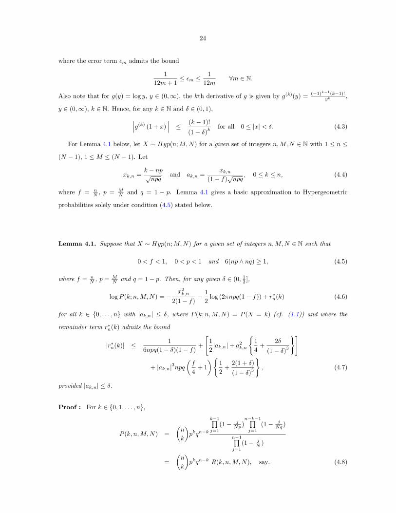
Lemma 4.1. Suppose that X ∼ Hyp(n;M,N) for a given set of integers n,M,N ∈ N such that
0 < f < 1, 0 < p < 1 and 6(np ∧ nq) ≥ 1, (4.5)
where f = nN , p = M
N and q = 1− p. Then, for any given δ ∈ (0, 12 ],
logP (k;n,M,N) = −x2
k,n
2(1− f)− 1
2log (2πnpq(1− f)) + r∗n(k) (4.6)
for all k ∈ 0, . . . , n with |ak,n| ≤ δ, where P (k;n,M,N) = P (X = k) (cf. (1.1)) and where the
remainder term r∗n(k) admits the bound
|r∗n(k)| ≤ 16npq(1− δ)(1− f)
+
[12|ak,n|+ a2
k,n
14
+2δ
(1− δ)3
]
+ |ak,n|3npq(f
4+ 1)
12
+2(1 + δ)(1− δ)3
, (4.7)
provided |ak,n| ≤ δ.
Proof : For k ∈ 0, 1, . . . , n,
P (k, n,M,N) =(n
k
)pkqn−k
k−1∏j=1
(1− jNp )
n−k−1∏j=1
(1− jNq )
n−1∏j=1
(1− jN )
=(n
k
)pkqn−k R(k, n,M,N), say. (4.8)

25
First consider R(k;n,M,N). By (4.2),
n−1∏j=1
(1− j
N) =
e(−N+εN )NN+ 12
e(−(N−n)+εN−n)(N − n)N−n+ 12
1Nn
=e(εN−εN−n)e−n
(1− f)N(1−f)+ 12,
k−1∏j=1
(1− j
Np)n−k−1∏
j=1
(1− j
Nq) =
e−neεNp−εNp−k+εNq−εNq−n+k
(1− kNp )Np−k+ 1
2 (1− n−kNq )Nq−n+k+ 1
2.
Note that by (4.4),
k
Np= f + xk,n
√fq
Npand
n− k
Nq= f − xk,n
√fp
Nq. (4.9)
Next write
zk,n =xk,n
√fpNq
1− f, yk,n =
xk,n
√fqNp
1− f(4.10)
and
ε∗ = εNp − εNp−k + εNq − εNq−n+k + εN−n − εN . (4.11)
Then R(k;n,M,N) can be expressed as,
logR(k;n,M,N) = ε∗ − log(1− f)2
−(Np(1− f)(1− yk,n) +
12
)log(1− yk,n)
−(Nq(1− f)(1 + zk,n) +
12
)log(1 + zk,n)
≡ ε∗ − log(1− f)2
−A1 −A2, say. (4.12)
Fix δ ∈ (0, 1/2). By Taylor’s expansion and (4.3),
A1 =(Np(1− f)(1− yk,n) +
12
)log(1− yk,n)
=(Np(1− f)(1− yk,n) +
12
)(−yk,n −
y2k,n
2+ r1n(k)
)
= −yk,n
(Np(1− f) +
12
)−y2
k,n
2
(12−Np(1− f)
)+ r2n(k),
(4.13)
where r1n(k) and r2n(k) are remainder terms, defined by the equality of the successive expressions. By
(4.3), for all n, k satisfying |yk,n| ≤ δ,
|r1n(k)| ≤ 2(1− δ)3
|yk,n|3
3!and, (4.14)
and
|r2n(k)| ≤ Np
2(1− f)|yk,n|3 +
∣∣∣∣Np(1− f)(1− yk,n) +12
∣∣∣∣ · |r1n(k)|. (4.15)

26
By similar arguments,
A2 =[Nq(1− f)(1 + zk,n) +
12
]log(1 + zk,n)
=(Nq(1− f) +
12
)zk,n +
z2k,n
2
[Nq(1− f)− 1
2
]+ r3n(k), (4.16)
where for all n, k, satisfying |zk,n| ≤ δ,
|r3n(k)| ≤ Nq(1− f)|zk,n|3
2+∣∣∣∣Nq(1− f)(1 + zk,n) +
12
∣∣∣∣ · |zk,n|3
3(1− δ)3, (4.17)
From, (4.12),(4.13) and (4.16), we have
logR(k;n,M,N) = ε∗ − log(1− f)2
−
[(zk,n − yk,n)
2+z2k,n
2
Nq(1− f)− 1
2
+y2
k,n
2
Np(1− f)− 1
2
+ r2n(k) + r3n(k)
]
= ε∗ − 12
log(1− f)−x2
k,nf
2(1− f)+ r4n(k), (4.18)
where for all n, k satisfying (|yk,n| ∨ |zk,n|) ≤ δ,
|r4n(k)| ≤ |r2n(k)|+ |r3n(k)|+ 12|yk,n − zk,n|+
14(y2
k,n + z2k,n
).
Next using Stirling’s formula on the binomial term, we have
log(
n
k
)pkqn−k
= log
e(εn−εk−εn−k)
√2πnpq
−(nq − xk,n
√npq +
12
)log
1− xk,n
√p
nq
−(np+ xk,n
√npq +
12
)log
1 + xk,n
√q
np
≡ ε∗∗ − log
√2πnpq −A3 −A4, say, (4.19)
where ε∗∗ = εn − εk − εn−k. Next write yk,n = xk,n
√p
nq and zk,n = xk,n
√q
np . Then, by arguments
similar to (4.13) and (4.16),
A3 =(nq − xk,n
√npq +
12
)log(
1− xk,n
√p
nq
)= −yk,n
(nq +
12
)+y2
k,n
2
(nq − 1
2
)+ r5n(k)
and
A4 =(np+ xk,n
√npq +
12
)log(
1 + xk,n
√q
np
)= zk,n
(np+
12
)+z2k,n
2
(np− 1
2
)+ r6n(k)

27
where for all k and n satisfying (|yk,n| ∨ |zk,n|) ≤ δ,
|r5n(k)|+ |r6n(k)|
≤ n
2
[q|yk,n|3 + p|zk,n|3
]+
2(1− δ)3
[(nq +
12
+ nq|yk,n|)|yk,n|3
+(np+
12
+ np|zk,n|)|zk,n|3
]. (4.20)
Hence, as in (4.18), it follows that
log(
n
k
)pkqn−k
= ε∗∗ − log
√2πnpq − 1
2x2
k,n + r7n(k) (4.21)
where for all n, k satisfying (|yk,n| ∨ |zk,n|) ≤ δ,
|r7n(k)| ≤∣∣∣∣12 (zk,n + yk,n)− 1
4(y2
k,n + z2k,n
) ∣∣∣∣+ |r5n(k)|+ |r6n(k)|.
Note that
fq + fp+ (1− f)p+ (1− f)q = 1,
(fq)2 + (fp)2 + ((1− f)p)2 + ((1− f)q)2 = (1− 2pq)(1− 2(1− f)) < 1,
and by (4.4), yk,n = fqak,n, zk,n = fpak,n, yk,n = (1 − f)pak,n, and zk,n = (1 − f)qak,n. Hence, it
follows that,
12|ak,n|+
14a2
k,n ≥ 12
(|yk,n|+ |yk,n|+ |zk,n|+ |zk,n|)
+14(y2
k,n + y2k,n + z2
k,n + z2k,n
). (4.22)
Now, combining (4.8), (4.18) and (4.20) and using (4.22) and the above identities, after some algebra,
we get
logP (k;n,M,N) = −x2
k,n
2(1− f)− 1
2log(2πnpq(1− f)) + r∗n(k),
where for all k, n satisfying |ak,n| ≤ δ,
|r∗n(k)− ε∗ − ε∗∗|
≤ |r4n(k)|+ |r7n(k)|
≤ npq
2|ak,n|3
[(1− f)(fq)2 + (1− f)(fp)2 + p2 + q2
]+
2npq(1− δ)3
|ak,n|3[(1− f)f2
(1 + δfq)q2
+ (1 + δfp)p2
+ (1 + δp)p2 + (1 + δq)q2]
+2
(1− δ)3|ak,n|3
12[(f3 + 1)(p3 + q3)
]+
12|ak,n|+
14a2
k,n
≤ 12|ak,n|+ a2
k,n
14
+2δ
(1− δ)3
+ |ak,n|3npq
(f
4+ 1)
12
+2(1 + δ)(1− δ)3
. (4.23)
28
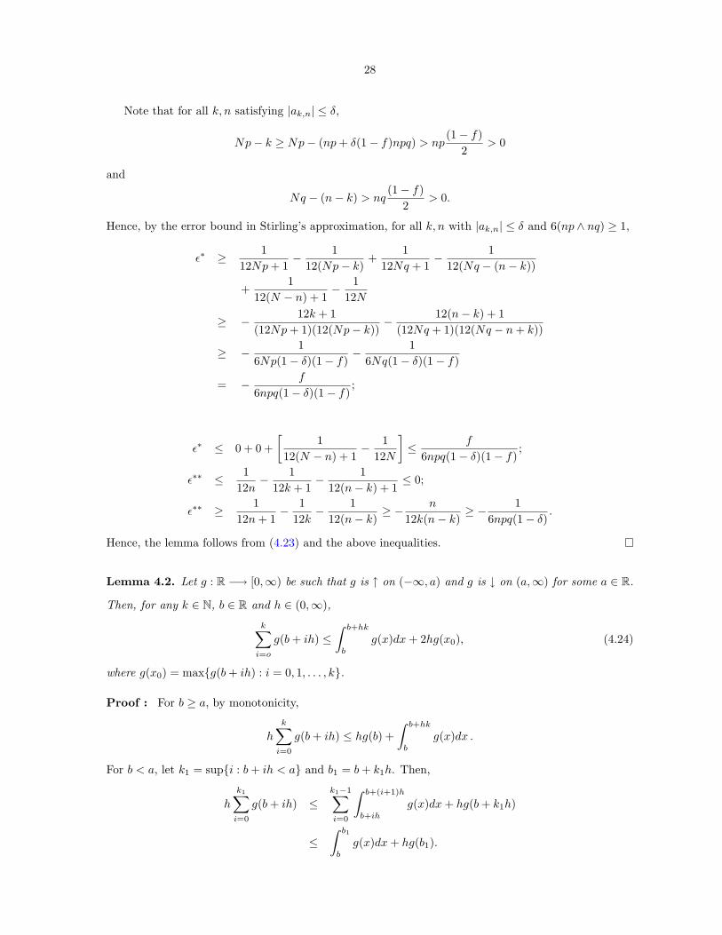
Note that for all k, n satisfying |ak,n| ≤ δ,
Np− k ≥ Np− (np+ δ(1− f)npq) > np(1− f)
2> 0
and
Nq − (n− k) > nq(1− f)
2> 0.
Hence, by the error bound in Stirling’s approximation, for all k, n with |ak,n| ≤ δ and 6(np ∧ nq) ≥ 1,
ε∗ ≥ 112Np+ 1
− 112(Np− k)
+1
12Nq + 1− 1
12(Nq − (n− k))
+1
12(N − n) + 1− 1
12N
≥ − 12k + 1(12Np+ 1)(12(Np− k))
− 12(n− k) + 1(12Nq + 1)(12(Nq − n+ k))
≥ − 16Np(1− δ)(1− f)
− 16Nq(1− δ)(1− f)
= − f
6npq(1− δ)(1− f);
ε∗ ≤ 0 + 0 +[
112(N − n) + 1
− 112N
]≤ f
6npq(1− δ)(1− f);
ε∗∗ ≤ 112n
− 112k + 1
− 112(n− k) + 1
≤ 0;
ε∗∗ ≥ 112n+ 1
− 112k
− 112(n− k)
≥ − n
12k(n− k)≥ − 1
6npq(1− δ).
Hence, the lemma follows from (4.23) and the above inequalities.
Lemma 4.2. Let g : R −→ [0,∞) be such that g is ↑ on (−∞, a) and g is ↓ on (a,∞) for some a ∈ R.
Then, for any k ∈ N, b ∈ R and h ∈ (0,∞),
k∑i=o
g(b+ ih) ≤∫ b+hk
b
g(x)dx+ 2hg(x0), (4.24)
where g(x0) = maxg(b+ ih) : i = 0, 1, . . . , k.
Proof : For b ≥ a, by monotonicity,
hk∑
i=0
g(b+ ih) ≤ hg(b) +∫ b+hk
b
g(x)dx .
For b < a, let k1 = supi : b+ ih < a and b1 = b+ k1h. Then,
h
k1∑i=0
g(b+ ih) ≤k1−1∑i=0
∫ b+(i+1)h
b+ih
g(x)dx+ hg(b+ k1h)
≤∫ b1
b
g(x)dx+ hg(b1).
29
Hence, for b < a and k > k1,
hk∑
i=0
g(b+ ih) = h
k1∑i=0
g(b+ ih) + hk∑
i=k1+1
g(b+ ih)
= h
k1∑i=0
g(b+ ih) + h
k−k1−1∑j=0
g(b1 + h+ jh)
≤∫ b1
b
g(x)dx+ hg(b1) + hg(b1 + h)
+∫ b1+h+(k−k1−1)h
b1+h
g(x)dx− hg(b1)
≤∫ b+hk
b
g(x)dx+ 2hg(x0).
For b < a and k < k1, it is easy to check (using the arguments above) that bound (4.24) trivially holds.
This completes the proof of the lemma.
Lemma 4.3. Let φ(x) = 1√2π
exp(−x2
2 ), x ∈ R. Then, for any h ∈ (0,∞), b ∈ [0,∞), j0 ∈ N,∣∣∣∣h j0∑i=0
φ(b+ ih)−∫ b+(j0+
12 )h
b−h2
φ(x)dx∣∣∣∣
≤ h2
12
[∫ b+j0h+ h2
b−h2
|φ′′(x)|dx
+ (4 + h) max|φ′′(x)| : b− h
2< x < b+ j0h+
h
2
]. (4.25)
Proof : Note that the function |φ′′(x)| = |x2−1|φ(x) is even, and on [0,∞), it is increasing on [1, 31/2]
and decreasing on each of the intervals [0, 1) and (31/2,∞), with the maximum value 1√2π
at x = 0 and
the minimum value 0 at x = 1. First suppose that (b− h2 , b+ (j0 + 1
2 )h) ∩ 0,√
3 = ∅. Then, writing
bi = b + ih, i ≥ 0, and using Taylor’s expansion, one can show that the leftside of (4.25) is bounded
above byj0∑
i=0
∣∣∣∣ ∫ bi+h2
bi−h2
(φ(x)− φ(bi)
)dx
∣∣∣∣≤ 1
2
j0∑i=0
∫ bi+h2
bi−h2
(x− bi)2
sup
y∈(bi−h2 ,bi+
h2 )
|φ′′(y)|
dx
≤ 12
j0∑i=0
(2∫ h
2
0
y2dy
)×∣∣∣∣φ′′ (bi − h
2
) ∣∣∣∣ ∨ ∣∣∣∣φ′′ (bi +h
2
) ∣∣∣∣
≤ h3
24
j0∑i=0
∣∣∣∣φ′′ (bi − h
2
) ∣∣∣∣+ ∣∣∣∣φ′′ (bi +h
2
) ∣∣∣∣
≤ h3
12
j0+1∑i=0
∣∣∣∣φ′′ (bi − h
2
) ∣∣∣∣ .

30
Hence by two applications of Lemma 4.2, one can show that
h
j0+1∑i=0
∣∣∣∣φ′′ (bi − h
2
) ∣∣∣∣ ≤∫ b+j0h+ h
2
b−h2
|φ′′(x)|dx
+ 4 max|φ′′(x)| : b− h
2≤ x ≤ b+ j0h+
h
2
.
Next consider the case where 0 ∈ [b− h2 , b+ h
2 ). Then, by Taylor’s expansion,∣∣∣∣∣hφ(b)−∫ b−h
2
b−h2
φ(x)dx
∣∣∣∣∣ ≤ h3|φ′′(0)|/24.
Now using similar arguments for the case ’√
3 ∈ (b− h2 , b+(j0 + 1
2 )h)’ and using the above bounds, one
can complete the proof of the lemma.
Proof of Theorem 2.1: Let r ∈ N be an integer such that (2.4) holds. Since r will be held fixed all
through the proof, we shall drop r from the notation for simplicity, and write fr = f , σr = σ, pr = p,
qr = q, nr − n, etc. First, suppose that f ≤ 12 . Consider the case x ≤ 0. Let xk = xk√
1−f= k−np
σ ,
k = 0, 1, . . . , n. Define
K0 = supk ∈ Z+ : xk ≤ 0
K1 = infk ∈ Z+ : xk ≥ −1
K2 = infk ∈ Z+ : xk ≥ −δσ and
Jx = bnp+ xσc, x ∈ R,
where δ ≡ δr ∈ (0, 12 ] is as in (2.3). Note that by definition,
K1 − 1 < np− σ ≤ K1, K2 − 1 < np− δσ2 ≤ K2,
xj ∈ [−1, 0]∀K1 ≤ j ≤ K0 and xj ∈ [−δσ,−1)∀K2 ≤ j < K1.
Hence, for any x ∈ [−δσ, 0],∣∣∣∣P (X − np
σ≤ x
)− Φ(x)
∣∣∣∣ = |P (X ≤ Jx)− Φ(x)|
≤ P (X < K2) +Jx∑
j=K2
∣∣∣∣P (X = j)− φ(xj)σ
∣∣∣∣+ ∣∣∣∣ Jx∑j=K2
φ(xj)σ
− Φ(x)∣∣∣∣
= I1 + I2 + I3, say. (4.26)
31
Consider I2 for x ∈ [−δσ,−1). Note that for x < −1, Jx−npσ ≤ x < −1. Hence Jx < K1 and xj < −1
for all j < Jx. From Lemma 4.1,
|r∗(j)| ≤ 16σ2(1− δ)
+
[|xj |2
2σ+|xj |2
σ2
14
+2δ
(1− δ)3
+|xj |3
2σA
]≡ r∗∗(j), (4.27)
where A = a1
(1 + 4(1+δ)
(1−δ)3
)and a1 ≡ a1r = f+4
4(1−f) (cf. (2.3)). For the given choice of δ, it is easy to
verify that δ ≤ 120 and δA < .59. Hence
|r∗(j)| ≤ (0.2)σ−2 +x2
j
2
[1σ
+2σ2
(0.3667) + δA
]≤ (0.2)σ−2 +
x2j
2
[min0.86,
65σ
+ 0.59]. (4.28)
Now, from (4.27), for all K2 ≤ j < K1,
|r∗(j)| ≤ (0.2)σ−2 + |xj |3∣∣∣∣ [ 1
2σ+
1σ2
(0.3667) +3a1
σ
]≤ 4|xj |3
a1
σ.
Next note that Jx−npσ ≤ x ∈ R, and∫ ∞
a
y3 exp(−by2
2)dy =
12b2
(1 + ba2)e−ba2for all a, b ∈ (0,∞),
and that for any a ∈ (0,∞), the function g(y; a) = y3 exp(−ay), y ∈ [0,∞), is increasing on [0,√
32a ],
and decreasing on (√
32a ,∞). Hence, by Lemmas 4.1 and 4.2, (4.28) and (4.29), with c = .07, we have
I2 ≤Jx∑
j=K2
∣∣∣∣φ(xj)σ
exp(r∗(j))− φ(xj)σ
∣∣∣∣≤ 1
σ
Jx∑j=K2
φ(xj)|r∗(j)| exp(|r∗(j)|)
≤ 4a1√2πσ2
exp(σ−2)Jx∑
j=K2
|xj |3 exp(−cx2j )
≤ 4a1 exp(σ−2)√2πσ
[ ∫ Jx−npσ
K2−npσ
|y|3 exp(−c|y|)dy
+2σ
max|y|3 exp(−c|y|) : K2 ≤ np+ σy ≤ Jx]
≤ C
σ(1− f)[(1 + x2) exp(−cx2)
]. (4.29)

32
Also, for −1 ≤ x ≤ 0, by Lemma 4.1,
∆1(x) ≡∣∣∣∣P (−1 ≤ X − np
σ≤ x
)−
K0∑j=K1
1σφ(xj)
∣∣∣∣≤
K0∑j=K1
∣∣∣∣P (X = j)− 1σφ(xj)
∣∣∣∣≤
K0∑j=K1
exp
(−x2
j
2
)|r∗(j)|exp(|r∗(j)|)√
2πσ.
For K1 ≤ j ≤ K0, from (4.27) and (4.28),
|r∗(j)| ≤[
12σ|xj |+ r∗∗(j)
]∧[
15σ2
+12σ
+1
2σ2(0.3667) +
A
2σ
]≤
[12σ
+1
5σ2+ (0.43)x2
j
]∧[
12σ
+1
5σ2+
0.3667σ2
+3a1
σ
]≤ 1
σ+[(.43)x2
j
]∧[4a1
σ
].
Hence, for −1 ≤ x ≤ 0, noting that K0 −K1 ≤ σ,
|∆1(x)| ≤K0∑
j=K1
exp(−x2j (0.07)) exp(σ−1)
5a1√2πσ2
≤ (K0 −K1) exp(σ−1)5a1√2πσ2
≤ C
σ. (4.30)
Thus, the bound (4.29) on I2 holds for all x ∈ [−δσ, 0]. Next consider I1. Note that for j ∈ 0, 1, . . . , n,
P (X = j + 1) T P (X = j)
⇔ Np− j
j + 1.
n− j
Nq − n+ j + 1T 1
⇔ j Sn(Np+ 1)N + 2
− Nq + 1N + 2
. (4.31)
Thus, P (X = j) < P (X = j + 1) for all 0 ≤ j ≤ np− 1. Hence, by (4.28) and Lemma 4.1,
I1 =K2−1∑j=0
P (X = j) < K2P (X = K2) ≤ K21σφ (xK2) exp(r∗(K2))
≤ K2√2πσ
exp(
15σ2
)exp(−x2
K2(.07))
≤ K2√2πσ
exp(
15σ2
)exp
(−(δσ − 1
σ
)2
(0.07)
)
≤ K2√2πσ
exp(−δ2σ2(0.07) + 2δ(0.07) + 0.13σ−2)
≤ np√2πσ
exp(−δ2σ2(0.07)) exp(0.014)
≤ (q(1− f))−1σ exp(−δ2σ2(0.07)).

33
It is easy to check that,
σ exp(−δ2σ2(0.07))(1 + x2) exp(−x2(0.07))
≤
2
(0.07)δ2σ : if x ∈ [0, δσ√2],
2δ2σ : if x ∈ [ δσ√
2, δσ].
Hence, it follows that for all x ∈ [−δa, 0],
I1 ≤ C
δ2qσ(1− f)(1 + x2) exp(−x2(0.07)). (4.32)
Since xJx ≤ x and xK2 ≤ −δσ + σ−1, by Lemma 4.3, for x ∈ [−δσ, 0], one gets
I3 ≤∣∣∣∣ 1σ
Jx∑j=K2
φ(xj)−∫ xJx+(2σ)−1
xK2−(2σ)−1φ(y)dy
∣∣∣∣+ ∣∣∣∣Φ(x)− Φ(xJx
+ (2σ)−1) ∣∣∣∣
+ Φ(xK2 − (2σ)−1
)≤ 1
12σ2
[∫ x+ 12σ
−∞|φ′′(y)|dy + 5 max
|φ′′(y)| : −∞ < y < x+
12σ
]
+ Φ(x+
12σ
)− Φ
(x− 1
2σ
)+ Φ(−δσ +
12σ
).
Note that for any a ∈ (0,∞),∫ ∞
a
y2e
(− y2
2
)dy ≤ 1
a
∫ ∞
a
y3e
(− y2
2
)dy =
2a
∫ ∞
a22
te−tdt =a2 + 2a
e−a22 ;
∫ ∞
a
y2e−y2
2 dy ≤∫ ∞
0
y2e−y2
2 dy ≤√π
2;
max|φ′′(y)| : a < y <∞ ≤ 1√
2πI(0 < a <
√3) + |φ
′′(a)|I(a ≥
√3);
And, for all a ∈ (0, δσ),
exp
(− (a− (2σ)−1)
2
2
)≤ exp
(−a
2
2+
a
2σ
)≤ exp
(−a
2
2+δ
2
).
Also note that, for 0 < a ≤ 1, b ∈ (0,∞),
1− Φ(b) ≤ 1bφ(b),
1− Φ(a) ≤∫ 1
a
φ(x)dx+ φ(1) ≤ φ(a)(1− a) + φ(a) = (2− a)φ(a).
Thus, for any x ∈ (0,∞),
Φ(x) ≤ e−x22 .

34
Since (2σ)−1< 1
8 and |y + (2σ)−1| ≤ |y| for y < − 18 , we have, for all x ∈ [−δa, 0],
I3 ≤ 112σ2
[2I(−2 ≤ x ≤ 0) + 5|x|φ
(x+
12σ
)I(−δσ ≤ x ≤ −2)
+ 5
1√2πI(−2 ≤ x ≤ 0) + (x2 + 1)φ
(x+
12σ
)I(−δσ ≤ x ≤ −2)
]+
1√2πσ
I(−2 ≤ x ≤ 0) +1σφ
(x+
12σ
)I(−δa ≤ x < −2)
+ Φ(−δσ +
12σ
)≤ 1
2σI(−2 ≤ x ≤ 0) + 2
x2 + 12σ2
+1σ
φ
(x+
12σ
)I(−δσ ≤ x ≤ −2)
+ exp
(−
(δσ − 12σ )2
2
)
≤ C
σ(1 + |x|) exp
(−x
2
2
). (4.33)
Next note that
P
(X − np
σ≤ x
)= 0 for all x < −np
σ
and for −npσ ≤ x ≤ −δσ,
P
(X − np
σ≤ x
)≤ I1 ≤ (q(1− f))−1
σ exp(−δ2σ2(0..07))
= (q(1− f))−1 (δσ)2
δ2σexp
(− δ2q2(1− f)2
[−npσ
]2(0.07)
)≤ (δ2q(1− f)σ)
−1|x|2 exp(− δ2q2(1− f)2x2(0.07)
).
Hence, for all x ≤ −δσ,
∣∣∣∣P (X − np
σ≤ x
)− Φ(x)
∣∣∣∣ ≤|x|2 exp(−δ2q2(1− f)2x2(0.07)) + exp
(−x2
2
)δq(1− f)σ
≤ 2δq(1− f)σ
x2 exp(− δ2q2(1− f)2x2(0.07)
).
(4.34)
Now using the fact that δ ∈[
245 ,
120
]for all f ∈ (0, 1
2 ], from (4.29),(4.30) and (4.32)-(4.34), it follows that
there exist numerical constants C1 and C2, not depending on n,M,N , such that for all x ∈ (−∞, 0],∣∣∣∣P (X − np
σ≤ x
)− Φ(x)
∣∣∣∣ ≤ C1
σq(1 + x2) exp(−C2qx
2),
provided δσ > 1. This proves (2.5) for x ∈ (−∞, 0] and f ≤ 12 . To prove the theorem for x ≥ 0 and
f ≤ 12 , define
Vr = nr −Xr, r ∈ N.
35
Note that Vr has a Hypergeometric distribution with parameters (nr, Nr −Mr, Nr). Further,
Xr − nrpr
σr= −Vr − nrqr
σr∀r ∈ N.
Hence, the derived bound on the right tails of Xr−nrpr
σr, can be obtained by repeating the arguments
above with Xr replaced by Vr and pr replaced by qr for any r such that δσr > 1. This proves (2.5) for
x ∈ [0,∞) and f ≤ 12 .
Next suppose that fr >12 . Consider the collection of Nr − nr objects that are left after the sample
of size nr has been selected from the population of size Nr. Let Yr =the number of ‘type A’-objects in
this collection. Then, for all r ∈ N and j ∈ Z,
Yr ∼ Hyp(Nr − nr;Mr, Nr), and P (Xr = j) = P (Yr = Mr − j).
(4.35)
Hence,
P (Xr ≤ k) =k∑
j=0
P (Xr = j) =k∑
j=0
P (Yr = Mr − j) = P (Yr ≥Mr − k).
Further, note that Var(Yr) = (Nr − nr)prqr
(1− Nr−nr
Nr
)= σ2
r . Hence, for each x ∈ R,
P
(Xr − nrpr
σr≤ x
)= P (Xr ≤ nrpr + xσr)
= P (Xr ≤ bnrpr + xσrc)
= P (Yr ≥Mr − bnrpr + xσrc)
= P (Yr ≥ xr) (say),
where Yr = Yr−(Nr−nr)pr
σrand xr = Mr−bnrpr+xσrc−(Nr−nr)pr
σr. Note that,
xr <1σr
[Nrpr − (nrpr + xσr − 1)−Nrpr + nrpr] = −x+ σ−1r
and similarly, xr ≥ −x. Hence, this implies,
P (Yr < xr) ≤ P (Yr ≤ xr) ≤ P (Yr ≤ −x+ σ−1r )
and
P (Yr < xr) ≥ P (Yr < −x) ≥ P (Yr ≤ −x− σ−1r ).

36
Now using the above identity and inequalities, we have∣∣∣∣P (Xr − nrpr
σr≤ x
)− Φ(x)
∣∣∣∣ = |P (Yr ≥ xr)− (1− Φ(−x))|
= |Φ(−x)− P (Yr < xr)|
≤ max|P (Yr ≤ −x− σ−1r )− Φ(−x− σ−1
r )|,
|P (Yr ≤ −x+ σ−1r )− Φ(−x+ σ−1
r )|
+ max|Φ(−x)− Φ(−x− σ−1r )|, |Φ(−x)− Φ(−x+ σ−1
r )|.
(4.36)
The proof of (2.5) for ‘f ∈ [ 12 , 1] and x ∈ R’ follows by replacing the above arguments with Xr, fr
replaced by Yr, 1− fr respectively and using the bound (4.35) and (4.36). This completes the proof of
the theorem.
Proof of Theorem 2.2: Use (2.5) and the inequality “exp(x) ≥ (1 + x) for all x ∈ (0,∞)”.

37
Figure 1 A plot of the cdfs of normalized Hypergeometric and Binomial ran-dom variables against the standard Normal cdf for the parametervalues N = 60, p = .5 and f = .5
x (Standardised)
y (C
DF
)
-5 0 5
0.0
0.2
0.4
0.6
0.8
1.0
HypergeometricBinomialNormal

38
Figure 2 A plot of the cdfs of normalized Hypergeometric and Binomial ran-dom variables against the standard Normal cdf for the parametervalues N = 200, p = .5 and f = .5
x (Standardised)
y (C
DF
)
-15 -10 -5 0 5 10 15
0.0
0.2
0.4
0.6
0.8
1.0
HypergeometricBinomialNormal

39
Figure 3 A plot of the cdfs of normalized Hypergeometric and Binomial ran-dom variables against the standard Normal cdf for the parametervalues N = 60, p = .9 and f = .7
x (Standardised)
y (C
DF
)
-20 -15 -10 -5 0
0.0
0.2
0.4
0.6
0.8
1.0
HypergeometricBinomialNormal
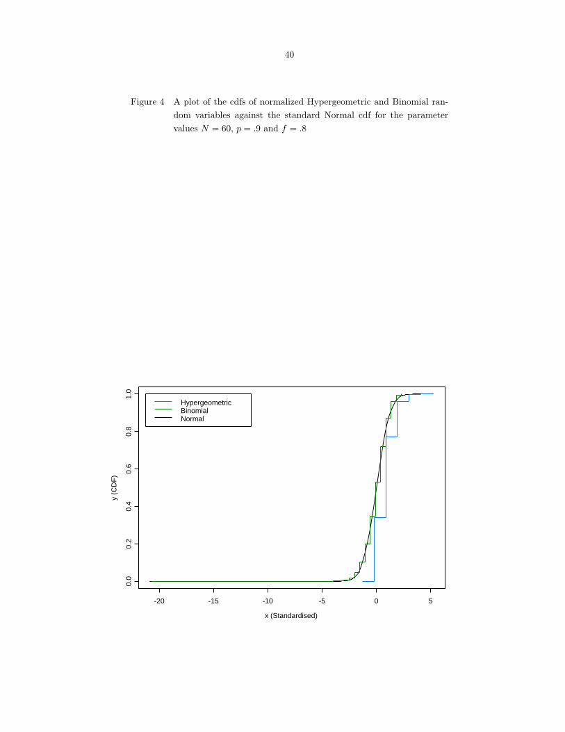
40
Figure 4 A plot of the cdfs of normalized Hypergeometric and Binomial ran-dom variables against the standard Normal cdf for the parametervalues N = 60, p = .9 and f = .8
x (Standardised)
y (C
DF
)
-20 -15 -10 -5 0 5
0.0
0.2
0.4
0.6
0.8
1.0
HypergeometricBinomialNormal
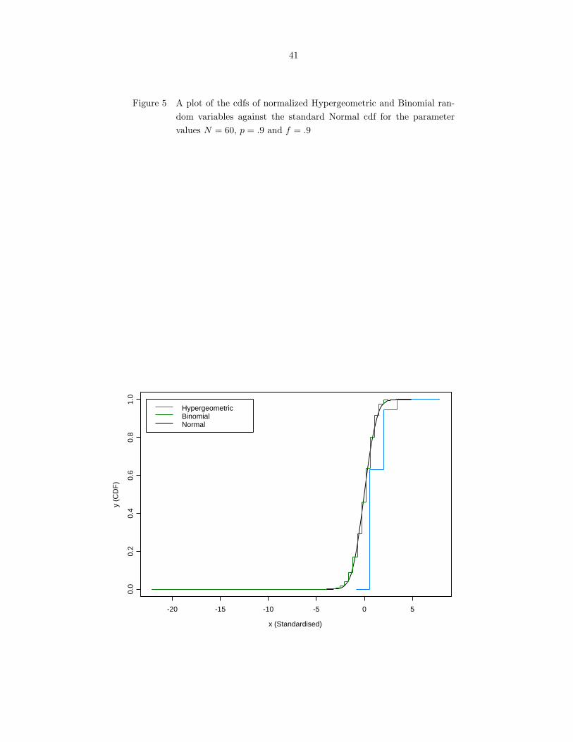
41
Figure 5 A plot of the cdfs of normalized Hypergeometric and Binomial ran-dom variables against the standard Normal cdf for the parametervalues N = 60, p = .9 and f = .9
x (Standardised)
y (C
DF
)
-20 -15 -10 -5 0 5
0.0
0.2
0.4
0.6
0.8
1.0
HypergeometricBinomialNormal
42
ASYMPTOTIC PROPERTIES OF SAMPLE QUANTILES FROM A
FINITE POPULATION
A paper to be submitted to Journal of Multivariate Analysis
Arindam Chatterjee
Abstract
In this paper we consider the problem of estimating quantiles of a finite population of size N on the
basis of a finite sample of size n selected without replacement. We prove the asymptotic normality of the
sample quantile and show that the scaled variance of the sample quantile converges to the asymptotic
variance under a slight moment condition. We also consider the performance of bootstrap in this
case proposed by Gross (1980). We show that Gross’s bootstrap method fails to be consistent, but a
suitably modified version of the bootstrapped quantile converges to the same asymptotic distribution
as the sample quantile. Consistency of the modified bootstrap variance estimate is also proved under
the same moment conditions.
1 Introduction
Estimation of quantiles of a finite population has been an important problem in survey sampling.
In this paper, we conduct a systematic and rigorous study of some important asymptotic properties
of the sample quantile when a simple random sample is selected without replacement from a finite
population. For complex sampling designs, Francisco and Fuller (1991) proved the asymptotic normality
of sample quantiles. Shao (1994) also proved the asymptotic normality of sample quantiles for stratified
multistage designs. In both the papers due to the complexity of the survey designs used, the conditions
imposed to prove the asymptotic normality are quite strong. In this paper we prove the asymptotic
normality of sample quantile under a superpopulation model, where all probability statements have a
43
clear interpretation, in terms of the underlying probability measure for the superpopulation. We also
show that the variance of the sample quantile converges almost surely under this probability measure
to the asymptotic variance under a mild moment and smoothness condition on the super-population
distribution function.
We also consider the performance of a bootstrap method that has been used in the finite population
context by Gross (1980). In both cases, the limiting sampling fraction f is allowed to take values in
[0, 1). The bootstrap provides a convenient way to estimate the variance of sample quantile in many
problems, because the usual techniques of linearization or jackknifing are not consistent for non-smooth
functionals like quantiles. We show that Gross’s version of the bootstrap fails if f > 0, i.e., if the sample
size grows as a nontrivial fraction of the population size. We also propose a modification and show that
the modified version of the bootstrap works for all values of f ∈ [0, 1). Specifically we show that the
cdf of the modified bootstrap quantile converges to the same asymptotic normal distribution and the
bootstrap variance of the sample quantile also converges in probability to the asymptotic variance.
2 Main Results
In order to have a suitable framework for developing asymptotic results in case of sampling from
a finite population, it is common to assume that the finite population is a random sample from a su-
perpopulation (see Isaki and Fuller (1982)). We assume that the superpopulation has an absolutely
continuous cdf F0 with density f0. Also denote the underlying probability measure of the superpopu-
lation as P0 and its corresponding expectation and variance as E0 and V0. Let r be a positive integer
valued variable, i.e. r takes values in N = 1, 2, . . .. We suppose that the population size N and
the sample size n, are indexed by r and grows to infinity. For each r ∈ N, let the finite population
XNr= X1, . . . , XNr
be an iid sample of size Nr selected from the superpopulation F0. We select a
simple random sample without replacement of size nr, Ynr= Y1, Y2, . . . , Ynr
from the finite population
XNr. The population and sample cdf’s are defined as,
FNr(t) =
1Nr
Nr∑j=1
1(Xj ≤ t), t ∈ R, (2.1)
and
Fnr(t) =
1nr
nr∑j=1
1(Yj ≤ t), t ∈ R, (2.2)
respectively, where 1(A) denotes the indicator function for a set A. The corresponding p-th sample
quantiles are ξp,Nr = F−1Nr
(p) and ξp,nr = F−1
nr(p). For all r ∈ N, define the standardized sample quantile
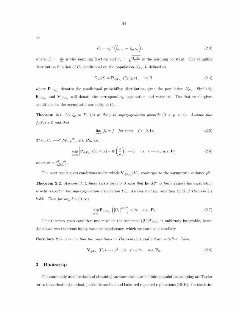
44
as,
Ur = a−1r
(ξp,nr − ξp,Nr
), (2.3)
where, fr = nr
Nris the sampling fraction and ar =
√1−fr
nris the norming constant. The sampling
distribution function of Ur conditional on the population XNr , is defined as
Gnr(t) = P·|XNr
(Ur ≤ t) , t ∈ R, (2.4)
where P·|XNrdenotes the conditional probability distribution given the population XNr
. Similarly
E.|XNrand V.|XNr
will denote the corresponding expectation and variance. The first result gives
conditions for the asymptotic normality of Ur.
Theorem 2.1. Let ξp = F−10 (p) be the p-th superpopulation quantile (0 < p < 1). Assume that
f0(ξp) > 0 and that
limr→∞
fr = f for some f ∈ [0, 1). (2.5)
Then, Ur −→d N(0, ρ2), a.s. P0, i.e.
supx∈R
∣∣∣∣P·|XNr(Ur ≤ x)− Φ
(x
ρ
) ∣∣∣∣→ 0, as r →∞, a.s. P0, (2.6)
where ρ2 = p(1−p)f20 (ξp)
.
The next result gives conditions under which V.|XNr(Ur) converges to the asymptotic variance ρ2.
Theorem 2.2. Assume that, there exists an α > 0 such that E0|X|α is finite (where the expectation
is with respect to the superpopulation distribution F0). Assume that the condition (2.5) of Theorem 2.1
holds. Then for any δ ∈ (0,∞)
supr≥1
E.|XNr
(∣∣Ur
∣∣2+δ)<∞ a.s.. P0 (2.7)
This theorem gives condition under which the sequence |Ur|2r≥1 is uniformly integrable, hence
the above two theorems imply variance consistency, which we state as a corollary.
Corollary 2.3. Assume that the conditions in Theorems 2.1 and 2.2 are satisfied. Then
V.|XNr(Ur) −→ ρ2 as r →∞, a.s. P0. (2.8)
3 Bootstrap
The commonly used methods of obtaining variance estimates in finite population sampling are Taylor
series (linearization) method, jackknife method and balanced repeated replications (BRR). For statistics

45
that can be expressed as smooth functions of sample means, consistency of variance estimators based
on these three methods were obtained by Krewski and Rao (1981). But, for non-smooth statistics such
as quantiles, the jackknife is not effective. Shao and Wu (1992) proved the consistency of the BRR
method for sample quantiles for stratified sampling. Another method used for variance estimation for
quantiles is the method suggested by Woodruff (1952). The consistency of this method was proved by
Francisco and Fuller (1991) and later by Shao (1994) under weaker conditions. Shao (1994) proved the
asymptotic normality sample quantile and constructed a consistent plug-in estimator of the asymptotic
variance by estimating the superpopulation density at the population quantile. In an important work,
Gross (1980) proposed using the bootstrap of Efron (1979) for estimating the variance of the sample
quantile in the finite population context. Although Gross (1980)’s work has been extensively referred to
the in the subsequent literature, the performance of bootstrap in estimating the asymptotic variance of
the quantile seems does not seem to be known. In this paper we show that Gross (1980)’s version of the
bootstrap fails whenever f > 0. However with proper rescaling, the bootstrapped quantile converges to
the same asymptotic normal distribution as the sample quantile for all f ∈ [0, 1). We also show that the
bootstrap variance estimate converges in probability to the asymptotic variance also, for all f ∈ [0, 1).
For the sake of completeness, we give a brief description of the bootstrap. Let Y∗nr= Y ∗
1 , . . . , Y∗nr
denote a bootstrap sample of size nr, selected with replacement from Ynr . The empirical cdf for the
bootstrap sample is
F∗nr
(t) =1nr
nr∑j=1
1(Y ∗j ≤ t) t ∈ R. (3.1)
The p-th bootstrap quantile is defined as ξ∗p,nr= F∗−1
nr(p). The bootstrap version of Ur conditioned on
the sample Ynris defined as (cf. Gross (1980))
U∗r = a−1
r
(ξ∗p,nr
− ξp,nr
). (3.2)
The next result shows that this version of the bootstrap fails for all f ∈ (0, 1).
Theorem 3.1. Suppose that condition (2.5) of the Theorem 2.1 holds. Then,
U∗r −→d N
(0,
ρ2
(1− f)
)a.s.(P0). (3.3)
Intuitively, this naive bootstrap fails because it does not account for the dependence in the sample
Ynr, which is obtained by sampling without replacement, while Y∗nr
is obtained by sampling with
replacement. However resampling without replacement is not feasible, as there is only one without
46
replacement sample of size nr from Ynr, viz. itself. A simple fix for this problem is to rescale and define
the new version of Ur as
U∗∗r = b−1
r
(ξ∗p,nr
− ξp,nr
), (3.4)
where b−1r = a−1
r
√1− f . The reason for re-scaling the bootstrap version of Ur is to make the bootstrap
version consistent in estimating the asymptotic variance. The corresponding bootstrap cdf is defined
as,
G∗nr
(t) = P∗ (U∗∗r ≤ t) , t ∈ R, (3.5)
where, P∗ is the bootstrap probability distribution conditioned on Ynr. Similarly E∗ and V∗ will denote
the bootstrap expectation and variance. The next result is about the asymptotic normality of U∗∗r and
consistency of the bootstrap variance estimator in estimating the asymptotic variance.
Theorem 3.2. Assume that condition (2.5) in Theorem 2.1 holds. Then
(a) U∗∗r −→d N(0, ρ2) in probability P0, where ρ2 = p(1−p)
f20 (ξp)
.
(b) If we assume that E0|X|α <∞ for some α > 0, then V∗(U∗∗r ) → ρ2 in probability P0.
4 Proofs
4.1 Auxiliary Results
We state the following Lemma’s that will be used in our proofs.
Lemma 4.1. (Singh (1981), Lemma 3.1) Let V1, . . . , Vk are iid with Vi = 1−a or −a with respective
probabilities a and 1− a, then for any k ≤ K, a ≤ B, Z ≤ D with ZKB ≤ D2 we have
P
(|
k∑i=1
Vi| > (1 + e/2)D
)≤ 2e−Z . (4.1)
Proof of Lemma 4.1: See Singh (1981).
Lemma 4.2. For any fixed t ∈ R,
limr→∞
1arFNr (ξp,Nr + tar)− FNr (ξp,Nr )− F0(ξp,Nr + tar) + F0(ξp,Nr ) = 0 a.s. P0. (4.2)
Proof of Lemma 4.2: Using the law of iterated logarithm for sample quantiles (Bahadur (1966)) we
can write,
ξp,Nr= ξp +O
(N−1/2
r (log logNr)1/2)a.s. (P0).
47
Define the quantity
∆Nr (y) ≡ FNr
(ξp +
y√Nr
+ tar
)− FNr
(ξp +
y√Nr
)− F0
(ξp +
y√Nr
+ tar
)+ F0
(ξp +
y√Nr
).
Also define ∆∗1,Nr
= sup∆Nr(y) : |y| ≤ logNr and ∆∗
2,Nr= inf∆Nr
(y) : |y| ≤ logNr. In order to
prove (4.2) it will be enough to show that
∆∗i,Nr
= o(ar) a.s. (P0) for i = 1, 2. (4.3)
Consider the intervals Bi =(
i−1√Nr, i√
Nr
], where |i| = 0, 1, . . . , (b
√Nr logNrc + 1). The union of Bi’s
covers the whole interval[−√Nr logNr,
√Nr logNr
]. So for any y ∈ Bi, we can write
∆Nr(y) ≤ FNr
(ξp +
i
Nr+ tar
)− FNr
(ξp +
i− 1Nr
)− F0
(ξp +
i− 1Nr
+ tar
)+ F0
(ξp +
i
Nr
)= ∆Nr
(i√Nr
)+ FNr
(ξp +
i
Nr
)− FNr
(ξp +
i− 1Nr
)+ F0
(ξp +
i
Nr+ tar
)− F0
(ξp +
i− 1Nr
+ tar
)= ∆Nr
(i√Nr
)+[FNr
(ξp +
i
Nr
)− F0
(ξp +
i
Nr
)− FNr
(ξp +
i− 1Nr
)+ F0
(ξp +
i− 1Nr
)]+ F0
(ξp + tar +
i
Nr
)− F0
(ξp + tar +
i− 1Nr
)+ F0
(ξp +
i
Nr
)− F0
(ξp +
i− 1Nr
)= ∆Nr
(i√Nr
)+ HNr
(i) + f0(θ1)1Nr
+ f0(θ2)1Nr
, (4.4)
where,
HNr(i) =
[FNr
(ξp +
i
Nr
)− F0
(ξp +
i
Nr
)− FNr
(ξp +
i− 1Nr
)+ F0
(ξp +
i− 1Nr
)], (4.5)
and θ1 ∈(ξp + tar + i−1
Nr, ξp + tar + i
Nr
)and θ2 ∈
(ξp + i−1
Nr, ξp + i
Nr
)(are obtained by using the
mean-value theorem). Let,
M = supf0(y) : |y − ξp| < δ0 (4.6)
be the supremum of f0 in some δ0-nbd of ξp. We can similarly obtain a lower bound on ∆Nr(y), so that
for all y ∈ Bi and for large enough r,
∆Nr
(i− 1√Nr
)−HNr (i)−
2MNr
≤ ∆Nr (y) ≤ ∆Nr
(i√Nr
)+ HNr (i) +
2MNr
. (4.7)
Note that (4.7) is also valid for all y ∈(−√Nr logNr − 1,−
√Nr logNr
). Initially we only consider the
upper bound for ∆Nr(y) in (4.7). Define, RNr
≡ max
∆Nr
(i√Nr
): |i| ≤ (b
√Nr logNrc+ 1)
. Then,
∆∗1,Nr
≤ RNr+ max
|i|≤(b√
Nr log Nrc+1)HNr
(i) +2MNr
.

48
Now choose a sequence εr : r ≥ 1, so that,
M
Nr εrar M, and εr → 0. (4.8)
The precise choice of εr will be determined later. For large r,
P0(∆∗1,Nr
> 4εrar) ≤ P0
(RNr
+ max|i|≤
√Nr log Nr
HNr(i) > 2εrar
)≤ P0 (RNr > εrar) + P0
(max
|i|≤√
Nr log Nr
HNr (i) > εrar
)≤
∑|i|≤
√Nr log Nr
P0
(∆Nr
(i√Nr
)> εrar
)+ P0 (HNr
(i) > εrar)
≤∑
|i|≤√
Nr log Nr
P0
(|∆Nr
(i√Nr
)| > εrar
)+ P0 (|HNr
(i)| > εrar)
=∑
|i|≤√
Nr log Nr
P0
∣∣∣∣ Nr∑j=1
ξj(i)
∣∣∣∣ > Nrεrar
+ P0
∣∣∣∣ Nr∑j=1
ξ′
j(i)
∣∣∣∣ > Nrεrar
= K1 +K2, (say), (4.9)
where, ξj(i) = 1(ξp + i
Nr< Xj ≤ ξp + i
Nr+ tar
)− pi and ξ
′
j(i) = 1(ξp + i−1
Nr< Xj ≤ ξp + i
Nr
)− p
′
i,
with pi = F0
(ξp + i
Nr+ tar
)− F0
(ξp + i
Nr
)and p
′
i = F0
(ξp + i
Nr
)− F0
(ξp + i−1
Nr
). Thus, for a
fixed i, ξj(i) : j = 1, . . . , Nr and ξ′j(i) : j = 1, . . . , Nr are iid random variables, with the following
distribution,
ξj(i) =
1− pi : w.p pi
pi : w.p 1− pi
and exactly same for ξ′
j(i) with p′
i. In order to find bounds on K1 and K2 in (4.9), we will use the
inequality derived in Singh (1981) (in Lemma 4.1 above). In this lemma, Z has to satisfy the bound
Z ≤(
D2
KB
)∧D
. For any large r and fixed t, and using mean value theorem we can choose B as the
upper bound of |pi| ≤M |t|ar ≡ B and K ≡ Nr. Let D ≡ Nrεrar
(1 + e
2
)−1. Then Z satisfies
Z ≤(1 +
e
2
)−1(
Nrε2rar
M |t|
)∧ (Nrεrar)
.
Since εr ↓ 0, a possible choice that satisfies the above constraint is Z =(1 + e
2
)−1(c2Nrε2rar)/|t|, for
some constant c2 (not depending on r). Using these choices of K,B,D and Z and using (4.1) in (4.9)
we have P0
(|∑Nr
j=1 ξj(i)| > Nrεrar
)≤ 2 exp(−Z), which gives a bound on K1,
K1 ≤ 4√Nr logNr exp
(−c2|t|−1
Nrε2rar
). (4.10)
Similarly for large r, |p′i| ≤ MNr
εrar ≡ B (see (4.8)). Using the same choices of K and D, we can
choose Z =(1 + e
2
)−1c3Nrεrar where c3 is some constant (not depending on r). Using this Z and

49
inequality (4.1) we can write,
K2 ≤ 4√Nr logNr exp(−c3Nrεrar). (4.11)
Now we choose the sequence εr as
ε3r =logNr
Nrar=
logNr√Nr(1− fr)
√fr. (4.12)
Using the condition (2.5) we can say that εr → 0. Also note that ε2rNrar = ε−1r logNr. Using the
relations (4.9)-(4.11) we can write,
∞∑r=1
P0
(∆∗
1,Nr> 4εrar
)≤
∞∑r=1
4√Nr logNr
[exp
(−c2
|t|Nrε
2rar
)+ exp (−c3Nrεrar)
]
=∞∑
r=1
4√Nr logNr
[exp
(−c2
|t|ε−1r logNr
)+ exp
(−c3(ε−2
r logNr))]
=∞∑
r=1
4√Nr logNr
[Nr
(−c2|t|−1ε−1r ) +Nr
(−c3ε−2r )]
< ∞, (4.13)
because ε−1r →∞ as r →∞. Using Borel-Cantelli lemma we have,
P0
(∆∗1,Nr
ar> 4εr i.o.
)= 0. (4.14)
This implies, ∆∗1,Nr
= o(ar) a.s. (P0). We can also conclude that RNr= o(ar) a.s. (P0) and
max|i|≤
√Nr log Nr
|HNr(i)| = o(ar) a.s. (P0).
From this it follows that ∆∗2,Nr
= o(ar) a.s. (P0). This completes the proof of the lemma.
Lemma 4.3. For each fixed t ∈ R, t 6= 0, define the quantities
pr,t = 1− qr,t = FNr(ξp,Nr
+ tar) and cr,t =√nr (pr,t − p)√
pr,t(1− pr,t)(1− fr). (4.15)
Assume that (2.5) holds. Then, for all 1 ≤ |t| ≤ logNr, there exists an r0 ∈ N such that for all r ≥ r0,
|cr,t| ≥ a|t|, (4.16)
with a = f0(ξp)2 and cr,t is as defined above in (4.15).
Proof of Lemma 4.3: Using the triangle inequality on (4.15) write
|cr,t| =|t|
√prqr
|I1r,t + I2r,t + I3r,t|
≥ |t|√pr,tqr,t
(|I1r,t| − |I2r,t| − |I3r,t|) . (4.17)
50
Note that for all |t| ≤ logNr, |tar| → 0. Thus we can use (4.24) to say that for large enough r and all
|t| ≤ logNr,
|I1r,t| ≥f0(ξp)
2(> 0).
Using Lemma (4.4) we can say that sup|I2r,t| : 1 ≤ |t| ≤ logNr → 0 a.s. (P0). And, since (Nrar)−1 ↓
0, we can say that |I3r,t| → 0 for all |t| ∈ [1, logNr]. Hence for a large r we can make (|I2r,t|+ |I3r,t|) <f0(ξp)
4 in the range 1 ≤ |t| ≤ logNr. We also use the fact that for any t, pr,t(1− pr,t)a.s.−→ p(1− p) ≤ 1
4 ,
so for r large (> r2),
|cr,t| ≥f0(ξp)
2|t|, (4.18)
which completes the proof of the lemma.
Lemma 4.4.
sup|t|≤log Nr
|FNr(ξp,Nr
+ tar)− FNr(ξp,Nr
)− F0 (ξp,Nr+ tar) + F0 (ξp,Nr
) | = o (ar) a.s. (P0). (4.19)
Proof of Lemma 4.4: The proof of this lemma closely follows the proof of Lemma 4.2. For all (y, t) :
|y|, |t| ≤ logNr, define
ΛNr (y, t) ≡ FNr
(ξp +
y√Nr
+thr√Nr
)− FNr
(ξp +
y√Nr
)− F0
(ξp +
y√Nr
+thr√Nr
)+ F0
(ξp +
y√Nr
),
where hr =√Nrar. Let Λ1,Nr = supΛNr (y, t) : |y|, |t| ≤ logNr and Λ2,Nr be the corresponding
infimum. Following earlier arguments used in the proof of Lemma 4.2 it will be enough to show
Λj,Nr= o(ar) a.s. (P0), for j = 1, 2. Define
R′
Nr= max
ΛNr
(i√Nr
,j√Nr
): |i|, |j| ≤ (b
√Nr logNrc+ 1)
.
51
For any y ∈(
i−1√Nr, i√
Nr
), t ∈
(j−1√
Nr, j√
Nr
)we can write
ΛNr(y, t)
≤ FNr
(ξp +
i
Nr+
j
Nrhr
)− FNr
(ξp +
i− 1Nr
)− F0
(ξp +
i− 1Nr
+j − 1Nr
hr
)+ F0
(ξp +
j
Nr
)= ΛNr
(i√Nr
,j√Nr
)+[FNr
(ξp +
i
Nr
)− FNr
(ξp +
i− 1Nr
)− F0
(ξp +
i
Nr
)+ F0
(ξp +
i− 1Nr
)]+[F0
(ξp +
i
Nr+
j
Nrhr
)− F0
(ξp +
i− 1Nr
+j − 1Nr
hr
)+ F0
(ξp +
i
Nr
)− F0
(ξp +
i− 1Nr
)]= ΛNr
(i√Nr
,j√Nr
)+ HNr (i) +
[F0
(ξp +
i
Nr+
j
Nrhr
)− F0
(ξp +
i
Nr+j − 1Nr
hr
)+ F0
(ξp +
i
Nr+j − 1Nr
hr
)− F0
(ξp +
i− 1Nr
+j − 1Nr
hr
)+ F0
(ξp +
i
Nr
)− F0
(ξp +
i− 1Nr
)]= ΛNr
(i√Nr
,j√Nr
)+ HNr
(i) +[f0(θ1)
hr
Nr+f0(θ2) + f0(θ3)
Nr
],
where HNr(i) is same as in (4.5) and
(θ1 − ξp − i
Nr
)∈(
j−1Nr
hr,j
Nrhr
),(θ2 − ξp − j−1
Nrhr
)∈(
i−1Nr, i
Nr
)and (θ3 − ξp) ∈
(i−1Nr, i
Nr
). Similarly we can find an lower bound
ΛNr (y, t) ≥ ΛNr
(i− 1Nr
,j − 1Nr
)−HNr (i)−
[f0(θ1)
hr
Nr+f0(θ2) + f0(θ3)
Nr
]And using the same arguments (about endpoints), we can say,
Λ1,Nr≤ RNr
+ max|i|≤(b
√Nr log Nrc+1)
HNr(i) +
M
Nr(2 + hr). (4.20)
Now choose a sequence εr ↓ 0 such that MNr
εrar. Let ηr =(εrar − Mhr
2Nr
). Then
P0(Λ1,Nr > 4εrar) ≤ P
(RNr + max
|i|≤(b√
Nr log Nrc+1)HNr (i) > 2ηr
)≤ P0(RNr
> ηr) + P0
(max
|i|≤(b√
Nr log Nrc+1)HNr
(i) > ηr
)= D1r +D2r (say).
Again we will use Lemma 3.1 by Singh (1981). Write, for all k = 1, . . . , Nr,
ψk(i,j) = 1(ξp +
i
Nr< Xk ≤ ξp +
i
Nr+
j
Nrhr
)− ri,j , and
ψ′
k(i) = 1(ξp +
i− 1Nr
< Xk ≤ ξp +i
Nr
)− r
′
i,
where ri,j = F0
(ξp + i
Nr+ j
Nrhr
)− F0(ξp + i
Nr) and r
′
i = F0(ξp + iNr
) − F0(ξp + i−1Nr
) for all (i, j).
Choose
ε−3r =
Nrar
(logNr)2 . (4.21)

52
Using the inequality (4.1) on the random variables ψk(i,j) with B ≡ Mhrlog Nr√
Nr, D ≡ Nrηr(1 + e
2 )−1
and Z = c1ε−1r logNr (c1 being some absolute positive constant) we can write
D1,r ≤∑
|i|,|j|≤(b√
Nr log Nrc+1)
P0
(∣∣∣∣ Nr∑k=1
ψk(i,j)
∣∣∣∣ > Nrηr
)
≤ 8Nr(logNr)2 exp
(−c1ε−1
r logNr
),
and use the same εr on the random variables ψ′k(i), with B ≡ MNr
, D ≡ Nrηr1
(1+ e2 )
and Z =
c2ε−2r (logNr)
2 (c2 being an absolute positive constant) we have
D2,r ≤∑
|i|≤(b√
Nr log Nrc+1)
P0
(∣∣∣∣ Nr∑k=1
ψ′
k(i)
∣∣∣∣ > Nrηr
)
≤ 4√Nr logNr exp
(−c2ε−2
r (logNr)2).
Since ε−1r ↑ ∞ (by condition (2.5)), the sum
∞∑r=1
P0 (Λ1,Nr> 4εrar)
≤∞∑
r=1
8Nr(logNr)
2 exp(−c1ε−1
r logNr
)+ 4√Nr logNr exp
(−c2ε−2
r (logNr)2)
< ∞.
By Borel-Cantelli lemma,
P0
(Λ1,Nr
ar> 4εr i.o
)= 0,
which gives Λ1,Nr= o(ar) a.s. (P0). From similar arguments as used in Lemma (4.2) we can also say
Λ2,Nr= o(ar) a.s. (P0). Combining them we have the proof of the lemma.
4.2 Proofs of the main results
Proof of Theorem 2.1: Let Zj = 1(Yj ≤ ξp,Nr + tar) for j = 1, . . . , nr. Then E.|XNr(Zj) = pr,t.
Then, the cdf of Ur can be written as
Gnr(t) = 1−P·|XNr
( ∑nr
j=1 (Zj − nrpr,t)√nrpr,t(1− pr,t)(1− fr)
< −cr,t
), (4.22)
Note that∑nr
j=1 Zj ∼ Hyp (nr;Nrpr,t, Nr), where the pmf of a random variable X ∼ Hyp (n;M,N) is
given as
P (X = x) ≡ P (x;n,M,N) =
(M
x )(N−Mn−x )
(Nn) if x = 0, 1 . . . , n
0 otherwise,

53
where, for any two integers r ≥ 1 and s,
(r
s
)=
r!
s!(r−s)! if 0 ≤ s ≤ r
0 otherwise.
We can write,
cr,t =t√
pr,t(1− pr,t)[I1r,t + I2r,t + I3r,t] , (4.23)
where,
I1r,t =F0(ξp,Nr
+ tar)− F0(ξp,Nr)
tar,
I2r,t =1t
FNr (ξp,Nr + tar)− FNr (ξp,Nr )− F0(ξp,Nr + tar) + F0(ξp,Nr )
ar
, and,
I3r,t =1tO
(1
Nrar
).
We are interested in finding the limiting value of cr,t. Using the Mean-Value theorem, we can write
I1r,t =F0(ξp,Nr
+ tar)− F0(ξp,Nr)
tar= f0(ξp,Nr + θrtar), (0 < θr < 1).
For a fixed t, we can use the fact that ξp,Nr→ ξp a.s. (P0), ar → 0 and the continuity of f0 in a
neighbourhood of ξp to say
I1r,t = f0(ξp,Nr+ θrtar) −→ f0(ξp) a.s. (P0). (4.24)
Using the result in Lemma 4.2 we can say, I2r,t → 0 a.s. (P0). And by (2.5), (Nrar)−1 → 0, which in
turn implies I3r,t → 0. Combining these we find that
pr,t − p
tar= [I1r,t + I2r,t + I3r,t] −→ f0(ξp) a.s. (P0).
Also from (4.23), we can write pr,t − p = tar [I1r + I2r + I3r]. Using same arguments, we can say that
pr,ta.s.−→ p (and hence qr,t
a.s.−→ q = 1− p). This gives
cr,t −→t
√pqf0(ξp) a.s. (P0). (4.25)
Using (4.22), write
∣∣Gnr(t)− Φ(t/ρ)
∣∣ ≤∣∣P·|XNr
( ∑nr
j=1 (Zj − nrpr,t)√nrpr,t(1− pr,t)(1− fr)
< −cr,t
)− Φ (−cr,t)
∣∣∣∣+∣∣Φ (cr,t)− Φ(t/ρ)
∣∣= A1,r +A2,r, (say).
Since (2.5) holds and pr,t → p almost surely (and p ∈ (0, 1)), we can say σ2r,t = V.|XNr
(∑nr
j=1 Zj) =
nrpr,t(1−pr,t)(1−fr) →∞. This ensures that we can use Theorem 2.2 of Lahiri and Chatterjee (2007),

54
which gives the following Berry-Esseen bound for Hypergeometric probabilities to bound the first term
A1,r (solely under the condition that σ2r,t →∞). Thus we can write
supu∈R
∣∣∣∣P·|XNr
( ∑nr
j=1 (Zj − nrpr,t)√nrpr,t(1− pr,t)(1− fr)
≤ u
)− Φ(u)
∣∣∣∣ ≤ C1√nrpr,tqr,t(1− fr)
, (4.26)
where C1 is some positive constant that does not depend on r. This ensures that A1,r → 0 a.s. (P0)
as r → ∞ for every t ∈ R. We use (4.25) and the continuity of Φ(·) to conclude that A2,r → 0 a.s.
(P0). Now restricting t over a countable dense subset of R, it follows that L (Ur|XNr ) −→d N(0, ρ2) as
r → ∞, a.s. (P0). In view of Polya’s theorem this completes the proof of both assertions in Theorem
2.1.
Proof of Theorem 2.2: For any r ∈ N and δ > 0, we can write
E.|XNr
(∣∣Ur
∣∣2+δ)
= (2 + δ)∫ ∞
0
t1+δP·|XNr
(a−1
r |ξp,nr− ξp,Nr
| > t)dt.
In order to prove (2.7) it will enough to show
supr∈N
∫ ∞
1
t1+δP·|XNr
(a−1
r |ξp,nr− ξp,Nr
| > t)dt <∞. (4.27)
Using the moment condition in Theorem 2.2 and Lemma 3 from Ghosh et al. (1984), applied to the
random variables X1, . . . , XNr, we can write, max|Xj | : 1 ≤ j ≤ Nr = o(N1/α
r ) with probability 1.
Since, max|Yj | : 1 ≤ j ≤ nr ≤ max|Xj | : 1 ≤ j ≤ Nr with probability 1, and we can say that
P0
(∫ ∞
N1/αr
t1+δP·|XNr
(a−1
r |ξp,nr− ξp,Nr
| > t)dt 6= 0 i.o.
)= 0.
For large r, we can write∫ N1/αr
1
t1+δP·|XNr
(a−1
r |ξp,nr− ξp,Nr
| > t)dt ≤
∫ log Nr
1
t1+δP·|XNr
(a−1
r |ξp,nr− ξp,Nr
| > t)dt
+N2+δ
αr P·|XNr
(a−1
r |ξp,nr − ξp,Nr | > logNr
)≡ B1 +B2 (say). (4.28)
Using (4.15) and (4.22), we have
P·|XNr
(|ξp,nr
− ξp,Nr| > tar
)= P·|XNr
(ξp,nr
> ξp,Nr+ tar
)+ P·|XNr
(ξp,nr
< ξp,Nr− tar
)= P·|XNr
(Znr,t < −cr,t) + 1−P·|XNr(Znr,−t < −cr,−t)
≤(P·|XNr
(|Znr,t| > cr,t))∧(P·|XNr
(|Znr,−t| > cr,−t)),
where Znr,t =∑nr
j=1(Zj−nrpr,t)√nrpr,t(1−pr,t)(1−fr)
. Using t ≡ logNr, we get the following
B2 ≤ N2+δ
αr
[P·|XNr
(|Znr,log Nr | > cr,log Nr ) + P·|XNr(|Znr,−log Nr | > cr,−log Nr )
].

55
We will use Corollary 2.4 of Lahiri et al. (2006) which gives an exponential upper bound on the tail prob-
abilities of a Hypergeometric random variable to bound the tail probabilities in the above expression.
The bound states that
P·|XNr(|Znr,t| ≥ u) ≤ C4
(pr,t ∧ qr,t)3 exp
(−C5u
2[pr,t ∧ qr,t]2), u ∈ R, (4.29)
where, C4, C5 are universal constants not depending on r and t is a fixed real number. Let
pr1 = FNr(ξp,Nr
+ (logNr)ar) and pr2 = FNr(ξp,Nr
− (logNr)ar) , (4.30)
with qrj = 1−prj , j = 1, 2, be similarly are similarly defined as pr,t by using t = ±(logNr) respectively.
Using (4.29) at these two values of t, we have following bounds
P·|XNr(|Znr,log Nr | > cr,log Nr ) ≤ C4
(pr1 ∧ qr1)3exp
(−C5(logNr)
2[pr1 ∧ qr1]2),
P·|XNr(|Znr,−log Nr
| > cr,−log Nr) ≤ C4
(pr2 ∧ qr2)3exp
(−C5(logNr)
2[pr2 ∧ qr2]2).
Thus B2 can be bounded by
B2 ≤ N2+δ
αr
C4
(pr,1 ∧ qr,1)3Nr
−(C5κ2[pr,1∧qr,1]2) +
C4
(pr,2 ∧ qr,2)3Nr
−(C5κ2[pr,2∧qr,2]2). (4.31)
Note that due to (2.5) we can say that logNrar → 0. Thus using the same arguments that we used in
proving pr,ta.s.−→ p (see (4.25)), we can say that (pr,j ∧ qr,j)
a.s.−→ (p ∧ q) as r → ∞ for j = 1, 2. Since
(p ∧ q) > 0, there exists some random R1 ∈ N (depending on the selected sample XNr), such that
0 < (p∧ q)/2 < (pr,j ∧ qr,j) for all r ≥ R1. Hence each term on the right side of (4.31) can be bounded,
for all r ≥ R1, by
N2+δ
αr
(pr,j ∧ qr,j)3Nr
−(C5k0[pr,j∧qr,j ]2) ≤ 8N
2+δα
r
(p ∧ q)3Nr
−C5(k0[p∧q]2)/4 ∀ j = 1, 2, (4.32)
where, k0 ∈ (0,∞) is such that2 + δ
α− C5
4k0(p ∧ q)2 < −1. (4.33)
For bounding the term in B1 we use Lemma 4.3 and the exponential bound (4.29). For any t ∈ [1, logNr]
we can write
P·|XNr(|Znr,t| > cr,t) ≤ P·|XNr
(|Znr,t| > a|t|)
≤ C4
(pr,t ∧ qr,t)3 exp
(−C5(at)
2[pr,t ∧ qr,t]2), and,
P·|XNr(|Znr,t| > cr,−t) ≤ C4
(pr,−t ∧ qr,−t)3 exp
(−C5(at)
2[pr,−t ∧ qr,−t]2).

56
where pr,t’s are similarly defined as in (4.15). Arguing similarly as before and making r large enough
(≥ R1) we can bound B1 as∫ √log Nr
1
t1+δP·|XNr
(a−1
r |ξp,nr− ξp,Nr
| > t)dt ≤ 2K1
∫ log Nr
1
t1+δ exp(−K2t2)dt, (4.34)
for some positive constants K1 and K2. For any choice of δ > 0, the integral on the right side of (4.34)
is finite. This shows that U2r : r ≥ 1 is uniformly integrable as claimed in (2.7).
Proof of Corollary 2.3: Using the results of Theorems 2.1 and 2.2, the proof of (2.8) follows.
Proof of Theorem 3.2(a): Define as earlier
pr,t = Fnr(ξp,nr
+ tbr) and dr,t =√nr(pr,t − p)√pr,t(1− pr,t)
. (4.35)
Let V′
j,t = 1(Y ∗
j ≤ ξp,nr+ tbr
)for j = 1, . . . , nr, with E∗(V
′
j,t) = pr,t. Then,
G∗nr
(t) = 1−P∗
(∑nr
j=1(V′
j,t − pr,t)√nrpr,t(1− pr,t)
< −dr,t
).
The Y ∗j are iid random variables and
∑nr
j=1 V′
j,t ∼ bin (nr, pr,t). We can use the Berry-Esseen theorem
for iid random variables to write
supu∈R
∣∣∣∣ P∗
(∑nr
j=1 V′
j,t − nrpr,t√nrpr,t(1− pr,t)
≤ u
)− Φ(u)
∣∣∣∣ ≤ C0√nrpr,t(1− pr,t)
, (4.36)
for some finite C0. Now consider the limiting value of dr,t. The numerator of dr,t can be written as,
√nr (pr,t − p) =
√nr
(Fnr (ξp,nr + tbr)− p
)=
√nr
(Fnr
(ξp,nr+ tbr)− Fnr
(ξp,nr))
+ O(n−1/2
r
)= J1r,t + J2r,t + O
(n−1/2
r
), (4.37)
where,
J1r,t =√nr
(FNr
(ξp,nr
+ tbr
)− FNr
(ξp,nr
))and,
J2r,t =√nr
(Fnr
(ξp,nr+ tbr)− FNr
(ξp,nr+ tbr) + FNr
(ξp,nr)− Fnr
(ξp,nr)).
We can split J1r,t into two parts as follows:
J1r,t =√nr
[F0(ξp,nr + tbr)− F0(ξp,nr )
]+√nr
[FNr
(ξp,nr+ tbr)− F0(ξp,nr
+ tbr) + F0(ξp,nr)− FNr
(ξp,nr)]
= J′
1r,t + J′′
1r,t (say).
57
For all r ≥ 1, define the set
Sr =|ξp,nr
− ξp| <2γr√nr
, (4.38)
where γr = log nr. Then,
P0(Scr) ≤ E0
(P·|XNr
(√nr|ξp,nr
− ξp,Nr| > γr)
)+ P0(
√nr|ξp,Nr
− ξp| > γr). (4.39)
Since we assumed that fr → f ∈ [0, 1), we can use the result in Theorem 2.1 to conclude that
√nr(ξp,nr
− ξp,Nr) −→d N(0, ρ2(1− f)) a.s. P0.
This implies, P·|XNr(√nr|ξp,nr
− ξp,Nr| > γr)− 2
(1− Φ
(γr
ρ√
1−f
))→ 0. Since γr →∞, by using DCT
we can conclude that
E0
(P·|XNr
(√nr|ξp,nr
− ξp,Nr| > γr)
)−→ 0. (4.40)
Using the CLT on quantiles for sampling from a continuous population we can say that√Nr (ξp,Nr
− ξp) →d
N(0, σ2) for some finite variance σ2. Using this fact the second term in (4.39) can be bounded,
P0(√nr|ξp,Nr − ξp| > γr) ≤ P0
(√Nr|ξp,Nr − ξp| >
γr√1 + fr
)→ 0, (4.41)
as r → ∞. Using (4.40) and (4.41) we can say that P0(Scr) → 0 as r → ∞. Using the mean-value
theorem we can write
J′
1r,t =√
1− fr√1− f
tf0(ξp,nr + θtbr),
for some θ ∈ (0, 1). Since fr → f , br → 0, γr√nr
↓ 0 and f0 is continuous, we can write for any ε > 0,
|J ′1r,t − tf0(ξp)| < ε, for large enough r. This implies
P0
(|J′
1r,t − tf0(ξp,nr)| > ε
)≤ P0
(|J′
1r,t − tf0(ξp,nr)| > ε
∩ Sr
)+ P0(Sc
r) → 0 as r →∞.
So, J′
1r,tP0−→ tf0(ξp) as r → ∞. Using the same argument as used in proving Lemma 4.2, we can say
that J′′
1r,tP0−→ 0 as r →∞. This implies that
J1r,tP0−→ tf0(ξp) as r →∞. (4.42)
Now we can write
J2r,t =1
√nr
nr∑j=1
(Wj −E.|XNr
(Wj)), (4.43)
where Wj = 1(ξp,nr
< Yj ≤ ξp,nr+ tbr
), j = 1, . . . , nr. Note that Wj = 1 or 0 with probabilities ωr,t =(
FNr(ξp,nr
+ tbr)− FNr(ξp,nr
))
and (1 − ωr,t) respectively. And∑nr
j=1Wj ∼ Hyp (nr; Nrωr,t, Nr).
We can write using Chebyshev’s inequality, for any ε > 0,
P0(|J2r,t| ≥ ε) = E0
(P·|XNr
(|J2r,t| ≥ ε))≤ E0
[V.|XNr
(J2r,t)ε2
]≤ E0
(ωr,t(1− ωr,t)(1− fr)
ε2
).
58
Now, ωr,tP0−→ 0 (this follows from the same arguments that lead to (4.42)). Using DCT it follows that
J2r,tP0−→ 0. (4.44)
We can also write, pr,tP0−→ p ∈ (0, 1). This implies
dr,tP0−→ tf0(ξp)√
pqas r →∞. (4.45)
Thus we have
∣∣ G∗nr
(t)− Φ(t/ρ)∣∣ ≤ ∣∣∣∣ P∗
(∑nr
j=1 V′
j,t − nrpr,t√nrpr,t(1− pr,t)
< −dr,t
)− Φ(−dr,t)
∣∣∣∣+ |Φ(dr,t)− Φ(t/ρ)|.
Now, using (4.36), the continuity of Φ(.) and (4.45) we can say that for all t ∈ R, G∗nr
(t) P0−→ Φ (t/ρ) as
r →∞. This completes the proof of Theorem 3.2.
Proof of Theorem 3.2(b): In order to show that the bootstrap variance converges to the asymptotic
variance it will be enough to show that |U∗∗r |2 : r ≥ 1 is uniformly integrable. This amounts to
showing that
supr≥1
∫ ∞
1
t1+δP∗(|U∗∗r | ≥ t)dt <∞, (4.46)
for some choice of δ > 0. By our earlier argument we can say that∫ ∞
n1/αr
t1+δP∗(|U∗∗r | ≥ t)dt→ 0 a.s. (P0) as r →∞.
We can write, P∗(|U∗∗r | ≥ t) = P∗(U∗∗
r ≥ t) + P∗(U∗∗r ≤ −t). Now divide the range of the integral in
(4.46) in two parts [1, log nr] and (log nr, n1/αr ) and write∫ n1/α
r
1
t1+δP∗(U∗∗r ≥ t) dt =
∫ log nr
1
+∫ n1/α
r
log nr
t1+δP∗(U∗∗r ≥ t) dt. (4.47)
Write the interval [1, log nr] =⋃
iGi, where Gi =(
i√nr, i+1√
nr
], 1 ≤ i ≤ b√nr log nrc. Also note that for
any t ∈ Gi, we can write,∫Gi
t1+δP∗(U∗∗r ≥ t) dt ≤
(i+ 1√nr
)1+δ
P∗
(U∗∗
r ≥ i√nr
).
We can also write P∗(U∗∗r ≥ t) = P∗
(V′
nr,t − pr,t < −(pr,t − p)). For notational simplicity write,
V′
nr(i) ≡ V
′
nr, i√nr
=1nr
nr∑j=1
1(Y ∗
j ≤ ξp,nr+
i√nr
br
)(4.48)
and
pr(i) ≡ pr, i√nr
= Fnr
(ξp,nr +
i√nr
br
). (4.49)

59
Thus,
∫ log nr
1
t1+δP∗(U∗∗r ≥ t) dt ≤
b√nr log nrc∑i=1
(i+ 1√nr
)1+δ
P∗
(U∗∗
r ≥ i√nr
)
=b√nr log nrc∑
i=1
(i+ 1√nr
)1+δ
P∗
(V′
nr(i)− pr(i) < −(pr(i)− p)
).(4.50)
From (4.37) we can write,
(pr(i)− p) =1
√nr
[J′
1r(i) + J′′
1r(i) + J2r(i)]
+O(n−1
r
),
where, J′
1r(i), J′′
1r(i), J2r(i) are similarly defined as in (4.48) and (4.49) by substituting t = i√nr
. Also
define Wj(i) in a similar way as Wj,t (see (4.43)). Now consider any ε > 0. We can write using
Hoeffding’s inequality (on the Wj(i)’s) for sampling without replacement (see Hoeffding (1963), Section
6),
P·|XNr
(max
1≤i≤b√nr log nrc
J2r(i)√nr
> ε
)≤
b√nr log nrc∑i=1
P·|XNr(J2r(i) ≥ ε
√nr)
≤b√nr log nrc∑
i=1
P·|XNr(|J2r(i)| ≥ ε
√nr)
=b√nr log nrc∑
i=1
P·|XNr
∣∣∣∣ nr∑j=1
(Wj(i)− pr(i))∣∣∣∣ > ε nr
≤ 2 exp(−2nrε
2)√nr log nr
→ 0 as r →∞. (4.51)
And hence,
maxJ2r(i)√nr
: 1 ≤ i ≤ b√nr log nrc
→ 0, (4.52)
in probability (P0). Also, again using Hoeffding’s inequality on J′′
1r(i)’s we get
P·|XNr
(max
1≤i≤b√nr log nrc|J′′
1r(i)| ≥ ε√nr
)
≤b√nr log nrc∑
i=1
P·|XNr
(|J′′
1r(i)| ≥ ε√nr
)
=∑
i
P·|XNr
∣∣∣∣ Nr∑j=1
1(ξp,nr < Xj ≤ ξp,nr +
ibr√nr
)−(
F0
(ξp,nr +
ibr√nr
)− F0(ξp,nr )
) ∣∣∣∣ ≥ εNr
≤ 2 exp(−2Nrε
2)√nr log nr
→ 0,
60
as r →∞. This shows that
max
J′′
1r(i)√nr
: 1 ≤ i ≤ b√nr log nrc
→ 0, (4.53)
in probability (P0). Using (4.52) and (4.53) we can say that whenever r ≥ r3(∈ N),
− (pr(i)− p) ≤ −J′
1r(i)2√nr, (4.54)
uniformly for all 1 ≤ i ≤ b√nr log nrc. Now,
J′
1r(i)√nr
= f0
(ξp,nr
+ θiibr√nr
)ibr√nr,
for some θi ∈ (0, 1). Since max∣∣ ibr√
nr
∣∣ : 1 ≤ i ≤ b√nr log nrc→ 0, hence using the same argument
(on the set Sr) we can say that f0(ξp,nr
+ θiibr√nr
)→ f0(ξp) in probability P0. Thus on the set Sr,
using Hoeffding’s inequality we can write
P∗
(V′
nr(i)− pr(i) < −(pr(i)− p)
)≤ P∗
(V′
nr(i)− pr(i) < −J
′
1r(i)2√nr
)
≤ P∗
(V′
nr(i)− pr(i) < −f0(ξp)
4ibr√nr
)≤ P∗
(|V
′
nr(i)− pr(i)| >
f0(ξp)4
ibr√nr
)≤ 2 exp
(−f
20 (ξp)8
i2b2r
)= 2 exp(−K3i
2b2r),
for some constant K3 (independent of i). Substituting this bound in (4.50), we have
∫ log nr
1
t1+δP∗(U∗∗r ≥ t) dt ≤
b√nr log nrc∑i=1
(i+ 1√nr
)1+δ
2 exp(−K3(ibr)2)
= O(1). (4.55)
The convergence follows from the convergence of the series∑∞
m=1m1+δ exp(−am2) (for any a, δ > 0).
Using i =√nr log nr, we can obtain the following bound for t = log nr,
P∗
(V′
nr,log nr− pr,log nr
< −(pr,log nr− p)
)≤ 2 exp
(−2K4(log nr)
2),
on the set Sr, where K4 is some finite constant. Then on the set Sr we can write,∫ n1/αr
log nr
t1+δP∗(U∗∗r ≥ t) dt ≤ K5n
2+δα
r exp(−2K4(log nr)
2)
= o(1), (4.56)

61
as r → ∞. Using (4.55) and (4.56) we can say that the integral in (4.47) is finite. We can similarly
deal with the integral involving P∗(U∗∗r ≤ −t). Combining both, we can show that |U∗∗
r |2 : r ≥ 1
is uniformly integrable. Note that P0(Scr) → 0 (shown earlier). Combining this with the asymptotic
normality we have V∗(U∗∗r ) → ρ2 in probability P0.

62
EDGEWORTH EXPANSIONS FOR SPECTRAL DENSITY ESTIMATES
A paper to be submitted to Journal of Time Series Analysis
Arindam Chatterjee and Soumendra N. Lahiri
Abstract
In this paper we obtain valid Edgeworth expansions for a class of spectral density estimators for a
stationary time series. The spectral estimators are based on tapered periodograms of overlapping blocks
of observations. We give conditions for the validity of a general order Edgeworth expansion under an
approximate strong mixing condition on the random variables, and also establish a moderate deviation
inequality. We also verify the conditions explicitly for linear time series, which are satisfied under mild
and easy-to-check conditions on the innovation variables and on their nonrandom co-efficients.
1 Introduction
Spectral densities play an important role in the frequency domain analysis of time series data. Accu-
rate estimation of the spectral density is therefore a central issue for eliciting second order characteristics
of a time series from the observed data. This has prompted a large amount of work on consistency and
asymptotic normality of spectral estimators. But, much less is known about higher order asymptotic
properties of spectral density estimators, which are most important for investigating accuracy of differ-
ent interval estimation methods for the spectral density. In this paper, we construct valid Edgeworth
expansions (EEs) for a class of lag-window spectral density estimators for a stationary time series. The
EE results of this paper can be used to study coverage accuracy of confidence intervals (CIs) resulting
from the standard Studentization approach and from R.A. Fisher’s Variance Stabilizing Transformation
(VST) approach, and also to investigate higher order properties of various block bootstrap CIs for the
spectral density.
63
Let Xt : t ∈ Z be a real valued time series with E(X1) = 0 and spectral density f(λ). Let
Xn = X1, . . . , Xn denote the observations from this time series. We construct an estimator of fn(λ)
based on blocks of observations from Xn. Let Xi,l = (Xi, . . . , Xi+l−1), i = 1, . . . , N = (n − l + 1),
denote a block of length l, where l ≡ ln ∈ [1, n] is some integer sequence with ln ↑ ∞ as n → ∞. Let
hr, r = 1, . . . , l be a data-taper. Based on the blocks Xi,l and the taper, the estimator fn(λ) is defined
as
fn(λ) =1N
N∑j=1
Yj,n, λ ∈ (−π, π), (1.1)
where, with ι =√−1,
Yj,n =
∣∣∣∑lr=1 hrXr+j−1 exp(ιλr)
∣∣∣22π∑l
r=1 h2r
(1.2)
denotes the tapered periodogram for the block Xj,l at frequency λ, j = 1, . . . , N . Thus, the estimator
fn(λ) is the average of the tapered periodograms over all blocks contained in X1, . . . , Xn . Estimators
of this type of are called lag-window spectral density estimators and were previously considered by
Bartlett (1946, 1950), Welch (1967), Brillinger (1975) and Zhurbenko (1979, 1980). These lag-window
estimators have a close connection with kernel based estimators pioneered by Grenander and Rosenblatt
(1957), Blackman and Tukey (1959) and Parzen (1961). It can be shown (see Priestley (1981)) by
computing a tapered periodogram of a block of observations with an appropriate choice of taper (lag-
window), we can obtain correspondence with kernel estimators.
The main results of the paper give valid EEs versions of the tapered spectral density estimator fn(λ)
under a set of regularity conditions on the process Xt. We also derive simple sufficient conditions
for the validity of the expansions when the time series is a linear process driven by a sequence of
independent and identically distributed (iid) random variables. These sufficient conditions only involve
the co-efficients of the linear process and the marginal distribution of the innovations and are easy to
verify. Unlike the case of the sample mean of independent or weakly dependent random variables, a
striking feature of the EEs here is that these are given by a series of terms in powers of b−1/2, where
b = o(n) (more precisely, b ∼ n/l as n → ∞). This is a consequence of the fact that the dependence
among neighboring overlapping blocks Xi,l’s is very strong, which leads to a behavior that is different
from sums of weakly dependent random variables. Indeed, the local strong dependence among the Yj,n
results in a slower rate of normal approximation for the spectral density estimator fn(λ). Therefore,
in this context, statements about second, third, ... order properties refer to those of the terms of
order b−1/2, b−1, etc. With this qualification, we also give explicit expressions for the polynomials in
the second- and third-order expansions, which are useful for constructing higher-order-accurate large
64
sample tests and CIs for f(·).
In an important work, Gotze and Hipp (1983) derived valid Edgeworth expansions for sample mean
of weakly dependent random variables. Extensions and refinements of their results for the sample mean
are given by Lahiri (1993) and Lahiri (1996). Janas (1994) derived valid EEs for a class of estimators,
known as the spectral mean estimators, for weighted integrals of the spectral density. Unlike the case of
the spectral density estimators, the spectral mean estimators are n1/2 consistent and are amenable to the
EE theory of Gotze and Hipp (1983), that gives expansions in powers of n−1/2. For the spectral density
itself, Velasco and Robinson (2001) recently constructed valid EEs for kernel based nonparametric
estimators of the spectral density (and also for studentized sample mean) for a Gaussian stationary
time series. In this paper, we drop the Gaussianity assumption and derive the EEs under the general
set-up introduced in Lahiri (2007) for EEs of estimators based on ’block’ variables.
The rest of the paper is organised as follows. Section 2 describes the condition used for deriving
the EE for the spectral density and provides simple sufficient conditions for linear processes. Section 3
gives the main results on the EE and moderate deviation bounds for the spectral density estimators.
Proofs of the results are given in Section 4.
2 Conditions for the Edgeworth Expansion
2.1 Theoretical framework and general conditions
To derive the EEs for the spectral density estimator for non-Gaussian processes, we adopt a frame-
work similar to Lahiri (2007) for sums of block variables, which is an extension of Gotze and Hipp
(1983)’s framework for sums of weakly dependent random variables. Suppose the Xt : t ∈ Z are
defined on a probability space (Ω,F , P ). Also suppose that Dj : j ∈ Z be a collection of sub σ-fields
of F . Let Dqp = σ〈Dj : j ∈ Z, p ≤ j ≤ q〉, −∞ ≤ p < q ≤ ∞. Let Zj,n = Yj,n − EYj,n, 1 ≤ j ≤ N
and let Wk,n = 1l
∑(kl∧N)j=(k−1)l+1 Zj,n, 1 ≤ k ≤ b0, where b0 ≡ b0n = dN/le, the smallest integer not less
than N/l. The Wk,n is a function (sample mean) of the block of variables Z(k−1)l+1,n, . . . , Zkl,n. Let
b ≡ bn = N/l. With this, the centered and scaled version of the spectral density estimator fn(λ) can
be written as
Tn(λ) =√b
1N
N∑j=1
(Yj,n −E(Yj,n))
=
1√b
b0∑k=1
Wk,n. (2.1)
We will use the following conditions.
65
(C.1) We assume that there exists a constant κ ∈ (0, 1) such that for all n > κ−1,
κ log n < l < κ−1n1−κ and max|hr| : r = 1, . . . , l < κ−1. (2.2)
(C.2) There exists a constant κ ∈ (0, 1] and an integer s ≥ 3 such that for all n ≥ κ−1,
maxE|Yj,n|(s+κ) : j = 1, . . . , N < κ−1. (2.3)
Further, λ ∈ [0, π), and limn→∞V(Tn(λ)) = σ2∞ exists and is non-zero.
(C.3) We assume that there exists a constant κ ∈ (0, 1) such that for all n,m > κ−1 and for all j ≥ 1,
1 ≤ i ≤ n, there exists a Dj+mj−m-measurable X†
j,m such that
E|Xj −X†j,m|
2 ≤ κ−1 exp(−κm). (2.4)
(C.4) There exists a constant κ ∈ (0, 1), such that for all n,m = 1, 2, . . ., and A ∈ Dn−∞ and B ∈ D∞
n+m,
|P(A ∩B)−P(A)P(B)| ≤ κ−1 exp(−κm). (2.5)
(C.5) There exists a constant κ ∈ (0, 1), such that for all i, j, k, r,m = 1, 2, . . ., and A ∈ Dij with
i < k < r < j and m > κ−1,
E∣∣∣∣P(A|Dj : j 6∈ [k, r])−P(A|Dj : j ∈ [i−m, k) ∪ (r, j +m])
∣∣∣∣ ≤ κ−1 exp(−κm). (2.6)
(C.6) There exist constants a ∈ (0,∞), κ ∈ (0, 1) and sequences mn ⊂ N and dn ⊂ [1,∞) with
m−1n +mnb
−1/2 = o(1), dn = O(l + ba) and d2nmn = O(b(1−κ)) such that for all n ≥ κ−1,
maxj0∈Jn
supt∈An
E∣∣∣∣Eexp
it j0+mn∑j=j0−mn
Wj,n
∣∣∣∣Dj0
∣∣∣∣ ≤ (1− κ), (2.7)
where Jn = mn +1, . . . , b−mn−1, An = t ∈ R : κdn ≤ |t| ≤ [ba + l](1+κ), and Dj0 = σ〈Dj :
j 6∈ [(j0 − bmn
2 c)l + 1, (j0 + bmn
2 c+ 1)l].
Condition (C.1) states the growth rate of the block size l and allows l to grow at a rate of O(n1−κ)
for arbitrarily small κ > 0. It also requires the taper-weights to be bounded, which is satisfied in
most applications. The first part of Condition (C.2) gives a sufficient condition for the existence of
(s + κ)-order absolute moment of the block variables Wk,n. Part (ii) of Condition (C.2) ensures that
asymptotic variance of Tn(λ) exists and is nonzero. By symmetry, this covers all λ ∈ (−π, π). Note
that the problem of existence of the asymptotic variance of Tn(λ), when the taper weights hr’s derive
from a taper function h : [0, 1] → R as
hr = h(r/l), r = 1, . . . , l. n ≥ 1, (2.8)

66
is well-studied and different sufficient conditions for (C.2) are available in the literature. A set of
sufficient conditions for this are given by (cf. Dahlhaus (1985)):
(i) h is continuously differentiable on [0,1] with∫ 1
0h2(x)dx ∈ (0,∞)
(ii) l = o(n) and
(iii) f, f4 are bounded and f is continuous at λ,
(2.9)
where f4 denotes the fourth order cumulant density of Xt. Note that in our set up, existence of a
bounded f4 is guaranteed if E|X1|4+κ < ∞ for some κ > 0 and (C.3)-(C.4) hold. Under (2.9), the
asymptotic variance of Tn(λ) is given by
σ2∞ = c2(h) · f2(λ)(1 + η(2λ)), (2.10)
where c2(h) = 2[ ∫ 1
0h(x)2dx
]−2 ∫ 1
0
[ ∫ 1−x
0h(y)h(x + y)dy
]2dx and η(ω) = 1 or 0 according as ω = 0
(mod 2π) or not.
Next consider the regularity conditions (namely (C.3)-(C.6)) that are exclusively used for deriving
the EEs for Tn(λ) here. Condition (C.3) is an approximation condition that connects the variables
Xj to the strong mixing property (C.4) of the auxiliary σ-fields Dj ’s. Thus, in our formulation, the
variables Xt are allowed to be only approximately strongly mixing. Condition (C.5) is an approximate
Markovian condition and is a variant of a similar condition used in Gotze and Hipp (1983). In particular,
this condition holds if the σ-fields Dj ’s have the Markov property. Finally, consider Condition (C.6),
which is a Cramer-type condition on the block variables Wj,n. In many applications, the natural choice
Dj = σ〈Xj〉 is not the most convenient for verifying (C.6), although this renders verification of (C.3)
trivial (e.g., with X†j,m = Xj for all j,m). A judicious choice of the auxiliary σ-fields Dj ’s often
facilitates the verification of (C.6). For examples of choices of Dj in different time series models, see
Gotze and Hipp (1983) and Lahiri (2003).
2.2 Sufficient conditions for linear processes
To give a specific example, we now consider an important case where Xt is a linear process and
derive simple sufficient conditions for (C.3)-(C.6). Thus, for the rest of this subsection, suppose that
Xt : t ∈ Z is a linear process, i.e.
Xt =∑k∈Z
εt−kak (2.11)
where εkk∈Z is a collection of iid random variables with Eε1 = 0 and Eε21 = σ2 ∈ (0,∞) and where
ak : k ∈ Z are real numbers satisfying
|ak| = O(|c1||k|) as n→∞, (2.12)
67
for some constant 0 < c1 < 1. For the process Xt in (2.11), we take Dj = σ〈εj〉, j ∈ Z. Then, the
σ-fields Dj ’s are independent and consequently, the strong-mixing condition (C.4) and the approximate
Markovian condition (C.5) on the Dj ’s hold trivially. To verify (C.3), we set
Xj,m =m∑
k=−m
εj−kak, j ∈ Z,m ≥ 1.
Then, it is evident from (2.11), (2.12) and the definition of Xj,m that Condition (C.3) holds. Next
consider condition (C.6). It turns out that by choosing the sequences dn and mn appropriately, the
conditional Cramer’s condition on the block-variables Wk,n can be ensured under some mild conditions
on the taper and under the following condition on the joint distribution of (ε1, ε21) :
lim supmax|t|,|s|→∞
∣∣∣E exp(ι[sε1 + tε21])∣∣∣ < 1. (2.13)
In particular, if the marginal distribution of ε1 has an absolutely continuous component (w.r.t. the
Lebesgue measure on the real line), then (2.13) holds. Thus, for the linear process in (2.11), the EE
results of this paper remain valid under some simple sufficient conditions on hr, ak and the marginal
distribution of ε1. The result is formally stated as Proposition 2.1 below and the proof is given in Section
4.
Proposition 2.1. Suppose that Xt is the linear process given by (2.11) and the taper weights hr :
r = 1, . . . , l are given by (2.8) for some function h satisfying (i) of (2.9). Also, suppose that for some
κ ∈ (0, 1) and an integer s ≥ 3, E|ε1|2(s+1)+κ < ∞, κ−1 log n < l < κ−1n(1−κ)/3, and ε1 satisfies
(2.13). If, in addition, f(λ)c2(h) > 0, then condition (C.1)-(C.6) hold for every a ∈ (0,∞) in (C.6),
and V(Tn(λ)) in (C.2) is given by V(Tn(λ)) = c2(h) · f2(λ)(1 + η(2λ)) (cf. (2.10)).
3 Edgeworth Expansion for the Spectral Density Function
3.1 Density of the Edgeworth Expansion
We define the Edgeworth polynomials pr,n(t) for t ∈ R by the identity (in u ∈ R)
exp
(s∑
r=3
(r!)−1ur−2b(r−2)/2χr,n(t)
)= 1 +
∞∑r=1
urpr,n(t), (3.14)
where χr,n(t) = trχr,n and χr,n is the r-th cumulant of Tn(λ) defined by the equation
ιrχr,n =dr
durlog E exp(ιuTn)
∣∣∣∣u=0
. (3.15)

68
The density of the (s− 2)-th order Edgeworth expansion ψs,n(x) of Tn(λ) is defined through its Fourier
transform ψs,n(t) ≡∫eιtxψs,n(x)dx, t ∈ R by
ψs,n(t) = exp(−χ2,n(t)/2)
[1 +
s−2∑r=1
b−r/2pr,n(ιt)
], t ∈ R. (3.16)
It can be shown (cf. Lemma 4.1, Lahiri (2007)) that under conditions (C.1)-(C.5), for any fixed t ∈ R,
the rth order cumulant χr,n(t) is O(b−(r−2)/2) for each 2 ≤ r ≤ s and hence, the co-efficients of the
polynomials pr,n(t), 2 ≤ r ≤ s are O(1) as n→∞. This shows that the density of the (s− 2)th order
EE for Tn = Tn(λ) is given by adding terms order O(b−r/2) for r = 1, . . . , s − 2 to a normal density
function.
It is worth noting that although the choice of the multiplier b(r−2)/2 in (3.14) is a natural one, by no
means it is unique. Indeed, b in (3.14) can be replaced by another factor b∗, say, such that b/b∗ = 1+o(1)
as n → ∞, without altering the functional form of the EE. This is because the terms b−r/2pr,n(t) in
(3.16) are invariant w.r.t. b, as implied by (3.14). To illustrate this fact and for future reference, we
now consider the special case s = 4 and write down the EE explicitly. Let µr,n = E(T rn(λ)). Since
E(Tn(λ)) = µ1,n = 0, µr,n = χr,n for all r = 1, 2, 3 and χ4,n = (µ4,n − µ22,n). Using the identity (3.14),
we find that
p1,n(t) =16b1/2t3χ3,n
p2,n(t) =124bt4χ4,n +
172bt6χ2
3,n (3.17)
which yields
ψ4,n(t) = exp(−t2µ2,n
2
)[1 +
(ιt)3
6µ3,n +
(ιt)4
24(µ4,n − µ2
2,n) +(ιt)6
72µ2
3,n
]. (3.18)
Note that the final expression only involves the cumulants of Tn and does not depend on the multi-
plicative factors b−r/2 explicitly. The density ψs,n(x) can now be found using the inversion formula
ψs,n(x) = (2π)−1 ∫R e
−ιtxψs,n(t)dt and the identity:[σ−kHk(σ−1x)
]φσ(x) = (2π)−1
∫R
exp(−ιtx)(ιt)kφσ(t)dt (3.19)
for all x ∈ R and k = 1, 2, . . ., where φσ(x) = (2π)σ2−1/2 exp(−x2/[2σ2]), x ∈ R and φσ(t) =
exp(−t2σ2/2), t ∈ R are the probability density function and the characteristic function of the N(0, σ2)
distribution, σ ∈ (0,∞), and where Hk(x) is the kth order Hermite polynomial. Thus,
ψ4,n(x) = φσn(x)
[1 +
µ3,n
6σ3n
H3(σ−1n x) +
(µ4,n − µ22,n)
24σ4n
H4(σ−1n x) +
µ23,n
72σ6n
H6(σ−1n x)
], (3.20)
where σ2n = µ2,n = V(Tn).
69
3.2 Main Results
We now state the EE results and a moderate deviation result for Tn under the conditions of Section
2.1. To that end, let s0 = 2bs/2c. For a Borel measurable function f : R → R and ε > 0, let
ω(f : ε) =∫
sup|f(x+ y)− f(x)| : |y| ≤ εφσ2∞
(x)dx,
where σ2∞ is as in condition (C.2). Let I(·) denote the indicator function. Then, we have the following
EE result for Tn(λ):
Theorem 3.1. Suppose that conditions (C.1)-(C.6) hold for some a ∈ ((s − 2)/2,∞). Let f : R → R
be a Borel measurable function with Mf ≡ sup(1 + |x|s0)−1|f(x)| : x ∈ R < ∞. Then, there exist
constants C1 = C1(a), C2 ∈ (0,∞) (neither depending on f) such that∣∣∣∣Ef(Tn(λ))−∫f(x)ψs,n(x)dx
∣∣∣∣ ≤ C1ω(f : b−a) + C2Mfb−(s−2)/2(log n)−2 (3.21)
for all n > C2, where f(x) = f(x)(1 + |x|s0)−1, x ∈ R.
As a corollary to the above theorem, we have the following result for the distribution function of
Tn(λ):
Corollary 3.2. Under the conditions of Theorem 3.1,
supu∈R
∣∣∣P(Tn(λ) ≤ u)−∫ u
−∞ψs,n(x)dx
∣∣∣ = O(b−(s−2)/2(log n)−2
). (3.22)
In some applications, e.g., for deriving stochastic approximations to the studentized sample mean,
where the studentization is ensured using the spectral density estimator fn(λ) (with λ = 0), moderate
deviation inequalities for the estimator fn(λ) are often very useful. Here we state a moderate deviation
bound for fn(λ) under the present framework that is valid without the conditional Cramer condition
(C.6).
Theorem 3.3. Suppose that conditions (C.1)-(C.5) hold. Then, for any γ ∈ (σ2∞,∞), there exists a
constant C3 ∈ (0,∞) (depending only on γ, s, κ, E|X1|s+κ) such that for all n ≥ 2,
E([
1 + |Tn(λ)|s0]I(|Tn(λ)| > [(s− 2)γ log n]1/2
))≤ C3b
−(s−2)/2(log n)−2. (3.23)

70
4 Proofs
Proof of Proposition 2.1: From the discussion in Section 2, it is evident that with the choice
Dj = σ〈εj〉, j ∈ Z, conditions (C.1)-(C.5) holds. Hence, we concentrate on verification of (C.6). The
tapered DFT dj(λ) for the set of observations in the j-th block Xj,l is
dj(λ) =l∑
r=1
hrXr+j−1 exp(ιλr)
=l∑
r=1
hr exp(ιλr)∑m∈Z
εmar+j−m−1
=∑m∈Z
εm
(l∑
r=1
hr exp(ιλr)ar+j−m−1
). (4.24)
For j,m ∈ Z, let
cjm =∑l
r=1 hr(cosλr)aj−m+r−1
[2π∑l
r=1 h2r]1/2
and sjm =∑l
r=1 hr(sinλr)aj−m+r−1
[2π∑l
r=1 h2r]1/2
.
Then, by (4.24), for any k ∈ Z and j ∈ 1, . . . , N, we can write
Yjn =(2π
l∑r=1
h2r
)−1∣∣∣dj(λ)∣∣∣2
=∣∣∣∣ ∑
m∈Zεm(cjm + ιsjm)
∣∣∣∣2
=
(∑
m∈Zεmcjm
)2
+
(∑m∈Z
εmsjm
)2
= ε2k(c2jk + s2jk) +An,j,−k + 2εkBn,j,−k, (4.25)
where,
An,j,−k ≡( ∑
m6=k
εmcjm
)2
+( ∑
m6=k
εmsjm
)2
, and
Bn,j,−k ≡ cjk
∑m6=k
εmcjm + sjk
∑m6=k
εmsjm.
are independent of εk.

71
Now setting k = j0l in (4.25), the sum in (2.7) is
j0+m∑j=j0−m
Wjn
=j0+m∑
j=j0−m
1l
jl∑i=(j−1)l+1
Yjn
=
1l
(j0+m)l∑j=(j0−m−1)l+1
Yjn
=1l
(j0+m)l∑j=(j0−m−1)l+1
[ε2k(c2jk + s2jk) + 2εkBn,j,−k +An,j,−k
]
= ε2k
1l
(j0+m)l∑j=(j0−m−1)l+1
(c2jk + s2jk)
+ 2εk
1l
(j0+m)l∑j=(j0−m−1)l+1
Bn,j,−k
+
1l
(j0+m)l∑j=(j0−m−1)l+1
An,j,−k
≡ en,kε
2k + 2Bn,−kεk +An,−k. (say), (4.26)
where en,k ≡ en is a constant (that does not depend on j0 and hence, on k) and where An,−k and Bn,−k
are random variables that are measurable with respect to (w.r.t) the σ-field D−k ≡ ∨j 6=kDj = σ〈εj :
j 6= k〉.
Next we consider the asymptotic behavior of en,k. Note that
en,k ≡ en
=(2πl
l∑r=1
h2r
)−1 ml∑j=−(m+1)l+1
[
l∑r=1
hr cos(λr)aj+r−1
]2
+
[l∑
r=1
hr sin(λr)aj+r−1
]2
=(2πl
l∑r=1
h2r
)−1 ml∑j=−(m+1)l+1
∣∣∣∣ l∑r=1
hr exp(ιλr)aj+r−1
∣∣∣∣2
=(2πl
l∑r=1
h2r
)−1 ml∑j=−(m+1)l+1
l∑r=1
l∑s=1
hrhseιλ(r−s)aj+r−1aj+s−1
=(2πl
l∑r=1
h2r
)−1 ml∑j=−(m+1)l+1
l−1∑p=−(l−1)
eιλp
l∧(l−p)∑s=1∨(1−p)
hshp+saj+s−1aj+p+s−1
=
(2πl
l∑r=1
h2r
)−1 l−1∑p=−(l−1)
eιλp
l∧(l−p)∑s=1∨(1−p)
hshs+p
∑j∈Z
ajaj+p +Rn(s, p)
. (4.27)
where, Rn(s, p) is defined by subtraction:
ml∑j=−(m+1)l+1
aj+s−1aj+p+s−1 =∑j∈Z
ajaj+p +Rn(s, p). (4.28)
72
Using the geometric rate of decay of the aj ’s for large |j| and Cauchy-Schwarz inequality, we get
sups=1,...,l
|p|≤(l−1)
|Rn(s, p)| ≤ sups=1,...,l
|p|≤(l−1)
∑j≤−(m+1)l+s
|ajaj+p|+∑
j>ml+s
|ajaj+p|
≤ sup
s=1,...,l
|p|≤(l−1)
∑j≤−ml
|aj ||aj+p|+∑
j≥ml+1
|aj ||aj+p|
≤ 2
∑|j|>(m−1)l
a2j
= O(c2(m−1)l1
)as n→∞. (4.29)
Since the bound on Rn(s, p) holds uniformly over all (s, p), by Cauchy-Schwarz inequality we get
(2πl
l∑r=1
h2r
)−1∣∣∣∣ l−1∑
p=−(l−1)
eιλp
l∧(l−p)∑s=1∨(1−p)
hshs+p Rn(s, p)∣∣∣∣
≤(2πl
l∑r=1
h2r
)−1 l−1∑p=−(l−1)
( l∑s=1
h2s
)∣∣∣Rn(s, p)∣∣∣
≤ 2l + 12πl
max|p|≤l−1
∣∣∣Rn(s, p)∣∣∣
= O(c2(m−1)l1
).
Thus, for m ≥ 2,
en =(2πl
l∑r=1
h2r
)−1 l−1∑p=−(l−1)
(l∧(l−p)∑
s=1∨(1−p)
hshs+p
)eιλp
∑j∈Z
ajaj+p
+O(cl1). (4.30)
Next let ω(δ) = sup|h(x) − h(y)| : |x − y| ≤ δ, x, y ∈ [0, 1], δ > 0. By the uniform continuity of
h(·) on [0, 1],
limδ↓0
ω(δ) = 0.
Hence, for hs = h(
sl
), 1 ≤ s ≤ l, by the bounded convergence theorem,
sup|p|2≤4l
∣∣∣∣∣∣l−1
l∧(l−p)∑s=1∨(1−p)
hshs+p −∫ 1
0
h(x)2dx
∣∣∣∣∣∣≤ sup
|p|2≤4l
∣∣∣∣∣∣l−1
l∧(l−p)∑s=1∨(1−p)
hshs+p − l−1l∑
s=1
h2s
∣∣∣∣∣∣+∣∣∣∣∣l−1
l∑s=1
h2s −
∫ 1
0
h(x)2dx
∣∣∣∣∣≤ ω
(2√l
l
)· l−1
l∑s=1
∣∣∣h(sl
)∣∣∣+ 4√l
l
(max
x∈[0,1]h(x)2
)+
∣∣∣∣∣l−1l∑
s=1
(sl
)2
−∫ 1
0
h(x)2dx
∣∣∣∣∣= o(1) as n→∞. (4.31)
73
Next, for any sequence amm∈Z, define the self-convolution sequence a∗a and the Fourier transform
a(·) of amm∈Z, respectively, as
(a ∗ a)(j) ≡∑p∈Z
apap+j , j ∈ Z and a(λ) =∑j∈Z
eιλjaj , λ ∈ [−π, π]. (4.32)
Then the Fourier transform of a ∗ a at frequency λ is given by
a ∗ a(λ) =∑j∈Z
eιλj(a ∗ a)(j)
=∑j∈Z
∑p∈Z
apap+jeιλ(j+p−p)
=∑p∈Z
ape−ιλp
∑j∈Z
aj+peιλ(j+p)
= |a(λ)|2. (4.33)
Thus, it follows that
∑|p|2≤4l
eιλp∑j∈Z
ajaj+p =∑p∈Z
∑j∈Z
ajaj+peιλp −
∑|p|2>4l
∑j∈Z
ajaj+peιλp
=∑p∈Z
(a ∗ a)(p)eιλp +O(c√
l1
)= |a(λ)|2 +O
(c√
l1
). (4.34)
The last term is of the order O(c√
l1
)because of the following:∣∣∣∣ ∑
|p|2>4l
∑j∈Z
ajaj+peιλp
∣∣∣∣ ≤∑
|p|2>4l
∑j∈Z
|ajaj+p|
≤∑|j|≤
√l
∑|p|2>4l
|ajaj+p|+∑|j|>
√l
∑|p|2≥4l
|ajaj+p|
≤ 2∑j∈Z
|aj |∑|p|2>l
|ap|
= O(c√
l1
)as l→∞, (4.35)
Thus combining equations (4.30)-(4.35), we can write∣∣∣∣∣∣∑
|p|≤(l−1)
eιλp∑j∈Z
ajaj+p
1l
l∧(l−p)∑s=1∨(1−p)
hshs+p
− |a(λ)|2∫ 1
0
h(x)2dx
∣∣∣∣∣∣≤
∣∣∣∣∣∣∑
|p|2≤4l
eιλp∑j∈Z
ajaj+p
1l
l∧(l−p)∑s=1∨(1−p)
hshs+p
− |a(λ)|2∫ 1
0
h(x)2dx
∣∣∣∣∣∣+∑
|p|2>4l
∑j∈Z
|ajaj+p| ·
(1l
l∑s=1
h2s
)= o(1) as n→∞

74
Consequently, it follows that
limn→∞
l · en =|a(λ)|2
2π6= 0 (as f(λ) 6= 0). (4.36)
Now set dn = l, mn = (log n)2, n ≥ 2. It is easy to verify that the requirements of condition (C.6)
on these sequences of constants hold, provided a ≥ 1/2. Now, by (4.36), the stationarity of Xt and
the Cramer’s condition on (ε21, ε1), there exists a κ ∈ (0, 1) such that
supj0∈Jn
supt∈An
E
∣∣∣∣∣∣Eexp
(ιt
j0+m∑j=j0−m
Wjn
)| D−j0l
∣∣∣∣∣∣≤ sup
j0∈Jn
supt∈An
E
∣∣∣∣∣∣Eexp
(ιt
j0+m∑j=j0−m
Wjn
)| D−j0l
∣∣∣∣∣∣≤ sup
j0∈Jn
supt≥l
E∣∣∣E( exp
(ιt[en,kε
2k + 2Bn,−kεk +An,−k]
)| εj : j 6= k
)∣∣∣≤ sup
t≥l,u∈R
∣∣∣E exp(ι[tenε
21 + uε1]
)∣∣∣≤ sup
t≥|a(λ)|2,u∈R
∣∣∣E( exp(ι[tε21 + uε1]
)∣∣∣≤ 1− κ,
for n large. Hence, condition (C.6) holds for all a ≥ 1/2.
Proof of Theorem 3.1: For proving Theorem 3.1, we shall use Theorem 2.1 of Lahiri (2007), which
gives conditions for valid EEs for the sum of block variables of the form
n−1n∑
j=1
Yjn
for zero mean variables Yjn = fjn(Xj,l), j = 1, . . . , n, where fjn’s are Borel measurable functions from
Rl → R and Xj,l = (Xj , . . . , Xj+l−1), j ≥ 1. To this end, we set Yjn = Yj,n − E(Yj,n) for j = 1, . . . , N
and Yjn = 0 for j = N + 1, . . . , n, where recall that N = n − l + 1 and where Yj,n’s are as defined
in (1.2). Then, it is easy to see that all the conditions in Theorem 2.1 of Lahiri (2007) are satisfied,
provided we show that:
limn→∞
V(∑n
j=1 Yjn)nl
exists and is nonzero (4.37)
and
E|Yjn − Y †jn,m| ≤ κ−1l exp(−κm) for all m > κ−1, (4.38)
for some κ ∈ (0, 1), where Y †jn,m is a random variable that is measurable w.r.t. σ〈Di : j − m ≤ i ≤
j +m+ l〉. Since l = o(n), by (C.2)
V(∑n
j=1 Yjn)nl
=N2V(Tn(λ)
[n/l]nl→ σ2
∞

75
as n→∞. Thus, the first condition above holds.
As for the second, define Y †jn,m by replacing Xt’s in the definition of Yj,n by X†
t,m’s, j = 1, . . . , N
and let Y †jn,m = 0 for j = N + 1, . . . , n. Then it follows that the Y †
jn,m is measurable w.r.t. σ〈Di :
j − m ≤ i ≤ j + m + l〉 for all j = 1, . . . , n. Further, by condition (C.3) and Cauchy-Schwarz and
Jensen’s inequalities,
supj=1,...,N
E|Yjn − Y †jn,m|
=( l∑
r=1
h2r
)−1
E
∣∣∣∣∣∣∣∣l∑
r=1
hrXr exp(ιλr)∣∣∣2 − ∣∣∣ l∑
r=1
hrX†r,m exp(ιλr)
∣∣∣2∣∣∣∣∣≤
( l∑r=1
h2r
)−1
×
E
(∣∣∣ l∑r=1
hrXr exp(ιλr)∣∣∣+ ∣∣∣ l∑
r=1
hrX†r,m exp(ιλr)
∣∣∣)2
1/2
×
E∣∣∣ l∑
r=1
hr(Xr −X†r,m)
∣∣∣21/2
≤ Cl exp(−κm)
for m large, for some constant C ∈ (0,∞). Hence, the second requirement also holds and the result
follows from Theorem 2.1 of Lahiri (2007).
Proof of Corollary 3.2 : Note that
supx∈R
|ω(I(−∞,x] : δ)| = O(δ)
as δ ↓ 0. Hence the result for the distribution function is implied by the Theorem 3.1 with f = I(−∞,x],
where IA denotes the indicator function of a set A.
Proof of Corollary 3.3 : Follows from Theorem 2.4 of Lahiri (2007) and the proof of Theorem
2.1 above.
76
BIBLIOGRAPHY
Bahadur, R. R. (1966). A note on quantiles in large samples. Ann. Math. Statist., 37:577–580.
Bartlett, M. S. (1946). On the theoretical specification and sampling properties of autocorrelated
time-series. Suppl J. Roy. Statist. Soc., 8:27–41.
Bartlett, M. S. (1950). Periodogram analysis and continuous spectra. Biometrika, 37:1–16.
Blackman, R. B. and Tukey, J. W. (1959). The measurement of power spectra: From the point of view
of communications engineering. Dover Publications Inc., New York.
Blyth, C. R. and Staudte, R. G. (1997). Hypothesis estimates and acceptability profiles for 2 × 2
contingency tables. J. Amer. Statist. Assoc., 92(438):694–699.
Brillinger, D. R. (1975). Time Series. Holt, Rinehart and Winston, Inc., New York. Data analysis and
theory, International Series in Decision Processes.
Burstein, H. (1975). Finite population correction for binomial confidence limits. Journal of the American
Statistical Association, 70:67–69.
Dahlhaus, R. (1985). On a spectral density estimate obtained by averaging periodograms. J. Appl.
Probab., 22(3):598–610.
Efron, B. (1979). Bootstrap methods: another look at the jackknife. Ann. Statist., 7(1):1–26.
Erdos, P. and Renyi, A. (1959). On the central limit theorem for samples from a finite population.
Magyar Tud. Akad. Mat. Kutato Int. Kozl., 4:49–61.
Feller, W. (1971). An introduction to probability theory and its applications. Vol. II. Second edition.
John Wiley & Sons Inc., New York.
Francisco, C. A. and Fuller, W. A. (1991). Quantile estimation with a complex survey design. Ann.
Statist., 19(1):454–469.
77
Ghosh, M., Parr, W. C., Singh, K., and Babu, G. J. (1984). A note on bootstrapping the sample
median. Ann. Statist., 12(3):1130–1135.
Gotze, F. and Hipp, C. (1983). Asymptotic expansions for sums of weakly dependent random vectors.
Z. Wahrsch. Verw. Gebiete, 64(2):211–239.
Grenander, U. and Rosenblatt, M. (1957). Statistical Analysis of Stationary Time Series. John Wiley
& Sons, New York.
Gross, S. T. (1980). Median estimation in sample surveys. In ASA Proceedings of the Section on Survey
Research Methods, pages 181–184.
Hajek, J. (1960). Limiting distributions in simple random sampling from a finite population. Magyar
Tud. Akad. Mat. Kutato Int. Kozl., 5:361–374.
Hoeffding, W. (1963). Probability inequalities for sums of bounded random variables. J. Amer. Statist.
Assoc., 58:13–30.
Isaki, C. T. and Fuller, W. A. (1982). Survey design under the regression superpopulation model. J.
Amer. Statist. Assoc., 77(377):89–96.
Janas, D. (1994). Edgeworth expansions for spectral mean estimates with applications to Whittle
estimates. Ann. Inst. Statist. Math., 46(4):667–682.
Krewski, D. and Rao, J. N. K. (1981). Inference from stratified samples: properties of the linearization,
jackknife and balanced repeated replication methods. Ann. Statist., 9(5):1010–1019.
Lahiri, S. N. (1993). Refinements in asymptotic expansions for sums of weakly dependent random
vectors. Ann. Probab., 21(2):791–799.
Lahiri, S. N. (1996). Asymptotic expansions for sums of random vectors under polynomial mixing rates.
Sankhya Ser. A, 58(2):206–224.
Lahiri, S. N. (2003). Resampling methods for Dependent data. Springer Series in Statistics. Springer-
Verlag, New York.
Lahiri, S. N. (2007). Asymptotic expansions for sums of block-variables under weak dependence. Ann.
Statist., 35(3).
Lahiri, S. N. and Chatterjee, A. (2007). A Berry-Esseen theorem for hypergeometric probabilities under
minimal conditions. Proc. Amer. Math. Soc., 135(5):1535–1545 (electronic).

78
Lahiri, S. N., Chatterjee, A., and Maiti, T. (2006). A sub-gaussian berry-esseen theorem for the
hypergeometric distribution. preprint available at http://arxiv.org/abs/math/0602276.
Madow, W. G. (1948). On the limiting distributions of estimates based on samples from finite universes.
Ann. Math. Statistics, 19:535–545.
Nicholson, W. L. (1956). On the normal approximation to the hypergeometric distribution. Ann. Math.
Statist., 27:471–483.
Parzen, E. (1961). Mathematical considerations in the estimation of spectra. Technometrics, 3:167–190.
Patel, J. K. and Samaranayake, V. A. (1991). Predictions intervals for some discrete distributions.
Journal of Quality Technology, 23:270–278.
Priestley, M. B. (1981). Spectral Analysis and Time Series. Vol. 2. Academic Press Inc. [Harcourt
Brace Jovanovich Publishers], London. Multivariate series, prediction and control, Probability and
Mathematical Statistics.
Seber, G. A. F. (1970). The effects of trap response on tag recapture estimates. Biometrics, 26:13–22.
Shao, J. (1994). L-statistics in complex survey problems. Ann. Statist., 22(2):946–967.
Shao, J. and Wu, C.-F. J. (1992). Asymptotic properties of the balanced repeated replication method
for sample quantiles. Ann. Statist., 20(3):1571–1593.
Singh, K. (1981). On the asymptotic accuracy of Efron’s bootstrap. Ann. Statist., 9(6):1187–1195.
Sohn, S. Y. (1997). Accelerated life-tests for intermittent destructive inspection, with logistic failure-
distribution. IEEE Transactions on Reliability, 46:122–129.
Velasco, C. and Robinson, P. M. (2001). Edgeworth expansions for spectral density estimates and
Studentized sample mean. Econometric Theory, 17(3):497–539.
von Collani, E. (1986). The α-optimal acceptance sampling scheme. Journal of Quality Technology,
18:63–66.
Welch, P. D. (1967). The use of Fast Fourier transform for the estimation of power spectra: A method
based on time averaging over short, modified periodograms. IEEE Trans. Audio. Electro. Acous.,
15(2):70–73.

79
Wendell, J. P. and Schmee, J. (1996). Exact inference for proportions from a stratified finite population.
J. Amer. Statist. Assoc., 91(434):825–830.
Wittes, J. T. (1972). On the bias and estimated variance of Chapman’s two-sample capture-recapture
population estimate. Biometrics, 28:592–597.
Woodruff, R. S. (1952). Confidence intervals for medians and other position measures. J. Amer. Statist.
Assoc., 47:635–646.
Zhurbenko, I. G. (1979). Spectral density estimates obtained by a time shift. Dokl. Akad. Nauk SSSR,
246(4):801–805.
Zhurbenko, I. G. (1980). On a limit theorem for statistics of spectral density with a time shift. Ukrain.
Mat. Zh., 32(4):463–476.


![ASYMPTOTIC EXPANSIONS FOR RATIOS OF PRODUCTS OF …downloads.hindawi.com/journals/ijmms/2003/953101.pdf · ASYMPTOTIC EXPANSIONS FOR RATIOS OF PRODUCTS... 1171 [3] R. B. Dingle, Asymptotic](https://img.pdfslide.us/doc/110x75/5f0746b27e708231d41c2ef3/asymptotic-expansions-for-ratios-of-products-of-asymptotic-expansions-for-ratios.jpg)