Embed Size (px)
Citation preview
Astronomy & Astrophysics manuscript no. PlanckMission2013 c© ESO 2014June 6, 2014
Planck 2013 results. I. Overview of products and scientific resultsPlanck Collaboration: P. A. R. Ade116, N. Aghanim79, M. I. R. Alves79, C. Armitage-Caplan122, M. Arnaud96, M. Ashdown93,8,
F. Atrio-Barandela23, J. Aumont79, H. Aussel96, C. Baccigalupi114, A. J. Banday128,13, R. B. Barreiro89, R. Barrena88, M. Bartelmann126,103,J. G. Bartlett1,91, N. Bartolo43, S. Basak114, E. Battaner131, R. Battye92, K. Benabed80,125, A. Benoıt77, A. Benoit-Levy32,80,125, J.-P. Bernard128,13,
M. Bersanelli47,68, B. Bertincourt79, M. Bethermin96, P. Bielewicz128,13,114, I. Bikmaev27,3, A. Blanchard128, J. Bobin96, J. J. Bock91,14,H. Bohringer104, A. Bonaldi92, L. Bonavera89, J. R. Bond11, J. Borrill18,119, F. R. Bouchet80,125, F. Boulanger79, H. Bourdin49, J. W. Bowyer75,
M. Bridges93,8,85, M. L. Brown92, M. Bucher1, R. Burenin118,107, C. Burigana67,45, R. C. Butler67, E. Calabrese122, B. Cappellini68,J.-F. Cardoso97,1,80, R. Carr54, P. Carvalho8, M. Casale54, G. Castex1, A. Catalano98,95, A. Challinor85,93,15, A. Chamballu96,20,79, R.-R. Chary76,
X. Chen76, H. C. Chiang37,9, L.-Y Chiang84, G. Chon104, P. R. Christensen110,51, E. Churazov103,118, S. Church121, M. Clemens63,D. L. Clements75, S. Colombi80,125, L. P. L. Colombo31,91, C. Combet98, B. Comis98, F. Couchot94, A. Coulais95, B. P. Crill91,111, M. Cruz25,
A. Curto8,89, F. Cuttaia67, A. Da Silva16, H. Dahle87, L. Danese114, R. D. Davies92, R. J. Davis92, P. de Bernardis46, A. de Rosa67, G. de Zotti63,114,T. Dechelette80, J. Delabrouille1, J.-M. Delouis80,125, J. Democles96, F.-X. Desert72, J. Dick114, C. Dickinson92, J. M. Diego89, K. Dolag130,103,
H. Dole79,78, S. Donzelli68, O. Dore91,14, M. Douspis79, A. Ducout80, J. Dunkley122, X. Dupac55, G. Efstathiou85, F. Elsner80,125, T. A. Enßlin103,H. K. Eriksen87, O. Fabre80, E. Falgarone95, M. C. Falvella6, Y. Fantaye87, J. Fergusson15, C. Filliard94, F. Finelli67,69, I. Flores-Cacho13,128,
S. Foley56, O. Forni128,13, P. Fosalba81, M. Frailis65, A. A. Fraisse37, E. Franceschi67, M. Freschi55, S. Fromenteau1,79, M. Frommert22,T. C. Gaier91, S. Galeotta65, J. Gallegos55, S. Galli80, B. Gandolfo56, K. Ganga1, C. Gauthier1,101, R. T. Genova-Santos88, T. Ghosh79,
M. Giard128,13, G. Giardino57, M. Gilfanov103,118, D. Girard98, Y. Giraud-Heraud1, E. Gjerløw87, J. Gonzalez-Nuevo89,114, K. M. Gorski91,132,S. Gratton93,85, A. Gregorio48,65, A. Gruppuso67, J. E. Gudmundsson37, J. Haissinski94, J. Hamann124, F. K. Hansen87, M. Hansen110,
D. Hanson105,91,11, D. L. Harrison85,93, A. Heavens75, G. Helou14, A. Hempel88,52, S. Henrot-Versille94, C. Hernandez-Monteagudo17,103,D. Herranz89, S. R. Hildebrandt14, E. Hivon80,125, S. Ho34, M. Hobson8, W. A. Holmes91, A. Hornstrup21, Z. Hou40, W. Hovest103, G. Huey42,K. M. Huffenberger35, G. Hurier79,98, S. Ilic79, A. H. Jaffe75, T. R. Jaffe128,13, J. Jasche80, J. Jewell91, W. C. Jones37, M. Juvela36, P. Kalberla7,
P. Kangaslahti91, E. Keihanen36, J. Kerp7, R. Keskitalo29,18, I. Khamitov123,27, K. Kiiveri36,61, J. Kim110, T. S. Kisner100, R. Kneissl53,10,J. Knoche103, L. Knox40, M. Kunz22,79,4, H. Kurki-Suonio36,61, F. Lacasa79, G. Lagache79, A. Lahteenmaki2,61, J.-M. Lamarre95, M. Langer79,
A. Lasenby8,93, M. Lattanzi45, R. J. Laureijs57, A. Lavabre94, C. R. Lawrence91, M. Le Jeune1, S. Leach114, J. P. Leahy92, R. Leonardi55,J. Leon-Tavares58,2, C. Leroy79,128,13, J. Lesgourgues124,113, A. Lewis33, C. Li102,103, A. Liddle115,33, M. Liguori43, P. B. Lilje87,
M. Linden-Vørnle21, V. Lindholm36,61, M. Lopez-Caniego89, S. Lowe92, P. M. Lubin41, J. F. Macıas-Perez98, C. J. MacTavish93, B. Maffei92,G. Maggio65, D. Maino47,68, N. Mandolesi67,6,45, A. Mangilli80, A. Marcos-Caballero89, D. Marinucci50, M. Maris65, F. Marleau83,
D. J. Marshall96, P. G. Martin11, E. Martınez-Gonzalez89, S. Masi46, M. Massardi66, S. Matarrese43, T. Matsumura14, F. Matthai103, L. Maurin1,P. Mazzotta49, A. McDonald56, J. D. McEwen32,108, P. McGehee76, S. Mei59,127,14, P. R. Meinhold41, A. Melchiorri46,70, J.-B. Melin20,
L. Mendes55, E. Menegoni46, A. Mennella47,68, M. Migliaccio85,93, K. Mikkelsen87, M. Millea40, R. Miniscalco56, S. Mitra74,91,M.-A. Miville-Deschenes79,11, D. Molinari44,67, A. Moneti80, L. Montier128,13, G. Morgante67, N. Morisset73, D. Mortlock75, A. Moss117,
D. Munshi116, J. A. Murphy109, P. Naselsky110,51, F. Nati46, P. Natoli45,5,67, M. Negrello63, N. P. H. Nesvadba79, C. B. Netterfield26,H. U. Nørgaard-Nielsen21, C. North116, F. Noviello92, D. Novikov75, I. Novikov110, I. J. O’Dwyer91, F. Orieux80, S. Osborne121, C. O’Sullivan109,
C. A. Oxborrow21, F. Paci114, L. Pagano46,70, F. Pajot79, R. Paladini76, S. Pandolfi49, D. Paoletti67,69, B. Partridge60, F. Pasian65, G. Patanchon1,P. Paykari96, D. Pearson91, T. J. Pearson14,76, M. Peel92, H. V. Peiris32, O. Perdereau94, L. Perotto98, F. Perrotta114, V. Pettorino22, F. Piacentini46,M. Piat1, E. Pierpaoli31, D. Pietrobon91, S. Plaszczynski94, P. Platania90, D. Pogosyan38, E. Pointecouteau128,13, G. Polenta5,64, N. Ponthieu79,72,
L. Popa82, T. Poutanen61,36,2, G. W. Pratt96, G. Prezeau14,91, S. Prunet80,125, J.-L. Puget79, A. R. Pullen91, J. P. Rachen28,103, B. Racine1,A. Rahlin37, C. Rath104, W. T. Reach129, R. Rebolo88,19,52, M. Reinecke103, M. Remazeilles92,79,1, C. Renault98, A. Renzi114, A. Riazuelo80,125,
S. Ricciardi67, T. Riller103, C. Ringeval86,80,125, I. Ristorcelli128,13, G. Robbers103, G. Rocha91,14, M. Roman1, C. Rosset1, M. Rossetti47,68,G. Roudier1,95,91, M. Rowan-Robinson75, J. A. Rubino-Martın88,52, B. Ruiz-Granados131, B. Rusholme76, E. Salerno12, M. Sandri67,
L. Sanselme98, D. Santos98, M. Savelainen36,61, G. Savini112, B. M. Schaefer126, F. Schiavon67, D. Scott30, M. D. Seiffert91,14, P. Serra79,E. P. S. Shellard15, K. Smith37, G. F. Smoot39,100,1, T. Souradeep74, L. D. Spencer116, J.-L. Starck96, V. Stolyarov8,93,120, R. Stompor1,
R. Sudiwala116, R. Sunyaev103,118, F. Sureau96, P. Sutter80, D. Sutton85,93, A.-S. Suur-Uski36,61, J.-F. Sygnet80, J. A. Tauber57, D. Tavagnacco65,48,D. Taylor54, L. Terenzi67, D. Texier54, L. Toffolatti24,89, M. Tomasi68, J.-P. Torre79, M. Tristram94, M. Tucci22,94, J. Tuovinen106, M. Turler73,
M. Tuttlebee56, G. Umana62, L. Valenziano67, J. Valiviita61,36,87, B. Van Tent99, J. Varis106, L. Vibert79, M. Viel65,71, P. Vielva89, F. Villa67,N. Vittorio49, L. A. Wade91, B. D. Wandelt80,125,42, C. Watson56, R. Watson92, I. K. Wehus91, N. Welikala1, J. Weller130, M. White39,
S. D. M. White103, A. Wilkinson92, B. Winkel7, J.-Q. Xia114, D. Yvon20, A. Zacchei65, J. P. Zibin30, and A. Zonca41
(Affiliations can be found after the references)
Received XX, 2012; accepted XX, 2013
ABSTRACTThe European Space Agency’s Planck satellite, dedicated to studying the early Universe and its subsequent evolution, was launched 14 May2009 and has been scanning the microwave and submillimetre sky continuously since 12 August 2009. In March 2013, ESA and the PlanckCollaboration released the initial cosmology products based on the the first 15.5 months of Planck data, along with a set of scientific and technicalpapers and a web-based explanatory supplement. This paper gives an overview of the mission and its performance, the processing, analysis, andcharacteristics of the data, the scientific results, and the science data products and papers in the release. The science products include maps ofthe cosmic microwave background (CMB) and diffuse extragalactic foregrounds, a catalogue of compact Galactic and extragalactic sources, anda list of sources detected through the Sunyaev-Zeldovich effect. The likelihood code used to assess cosmological models against the Planck dataand a lensing likelihood are described. Scientific results include robust support for the standard six-parameter ΛCDM model of cosmology andimproved measurements of its parameters, including a highly significant deviation from scale invariance of the primordial power spectrum. ThePlanck values for these parameters and others derived from them are significantly different from those previously determined. Several large-scaleanomalies in the temperature distribution of the CMB, first detected by WMAP, are confirmed with higher confidence. Planck sets new limits onthe number and mass of neutrinos, and has measured gravitational lensing of CMB anisotropies at greater than 25σ. Planck finds no evidencefor non-Gaussianity in the CMB. Planck’s results agree well with results from the measurements of baryon acoustic oscillations. Planck finds alower Hubble constant than found in some more local measures. Some tension is also present between the amplitude of matter fluctuations (σ8)derived from CMB data and that derived from Sunyaev-Zeldovich data. ThePlanck and WMAP power spectra are offset from each other by anaverage level of about 2% around the first acoustic peak. Analysis of Planck polarization data is not yet mature, therefore polarization results arenot released, although the robust detection of E-mode polarization around CMB hot and cold spots is shown graphically.
Key words. Cosmology: observations — Cosmic background radiation — Surveys — Space vehicles: instruments — Instrumentation: detectors
1
arX
iv:1
303.
5062
v2 [
astr
o-ph
.CO
] 5
Jun
201
4
1. Introduction
The Planck satellite1 (Tauber et al. 2010a; Planck CollaborationI 2011) was launched on 14 May 2009 and observed the skystably and continuously from 12 August 2009 to 23 October2013. Planck’s scientific payload comprised an array of 74 de-tectors sensitive to frequencies between 25 and 1000 GHz, whichscanned the sky with angular resolution between 33′ and 5′.The detectors of the Low Frequency Instrument (LFI; Bersanelliet al. 2010; Mennella et al. 2011) are pseudo-correlation ra-diometers, covering bands centred at 30, 44, and 70 GHz. Thedetectors of the High Frequency Instrument (HFI; Lamarre et al.2010; Planck HFI Core Team 2011a) are bolometers, coveringbands centred at 100, 143, 217, 353, 545, and 857 GHz. Planckimages the whole sky twice in one year, with a combination ofsensitivity, angular resolution, and frequency coverage never be-fore achieved. Planck, its payload, and its performance as pre-dicted at the time of launch are described in 13 papers includedin a special issue of Astronomy & Astrophysics (Volume 520).
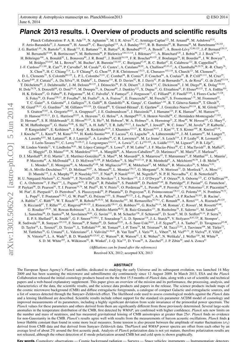
The main objective of Planck, defined in 1995, is to mea-sure the spatial anisotropies in the temperature of the cos-mic microwave background (CMB), with an accuracy set byfundamental astrophysical limits, thereby extracting essentiallyall the cosmological information embedded in the temperatureanisotropies of the CMB. Planck was also designed to measureto high accuracy the CMB polarization anisotropies, which en-code not only a wealth of cosmological information, but alsoprovide a unique probe of the early history of the Universe dur-ing the time when the first stars and galaxies formed. Finally,Planck produces a wealth of information on the properties of ex-tragalactic sources and on the dust and gas in the Milky Way(see Fig. 1). The scientific objectives of Planck are described indetail in Planck Collaboration (2005). With the results presentedhere and in a series of accompanying papers (see Fig. 2), Planckhas already achieved many of its planned science goals.
This paper presents an overview of the Planck mission, andthe main data products and scientific results of Planck’s secondrelease2, based on data acquired in the period 12 August 2009 to28 November 2010.
1.1. Overview of 2013 science results
Cosmology—A major goal of Planck is to measure the key cos-mological parameters describing our Universe. Planck’s com-bination of sensitivity, angular resolution, and frequency cov-erage enables it to measure anisotropies on intermediate andsmall angular scales over the whole sky much more accuratelythan previous experiments. This leads to improved constraintson individual parameters, the breaking of degeneracies between
1 Planck (http://www.esa.int/Planck) is a project of the EuropeanSpace Agency (ESA) with instruments provided by two scientific con-sortia funded by ESA member states (in particular the lead countries,France and Italy) with contributions from NASA (USA), and telescopereflectors provided in a collaboration between ESA and a scientific con-sortium led and funded by Denmark.
2 In January of 2011, ESA and the Planck Collaboration releasedto the public a first set of scientific data, the Early Release CompactSource Catalogue (ERCSC), a list of unresolved and compact sourcesextracted from the first complete all-sky survey carried out by Planck(Planck Collaboration VII 2011). At the same time, initial scientific re-sults related to astrophysical foregrounds were published in a specialissue of Astronomy and Astrophysics (Vol 520, 2011). Since then, 12“Intermediate” papers have been submitted for publication to A&A con-taining further astrophysical investigations by the Collaboration.
combinations of other parameters, and less reliance on supple-mentary astrophysical data than previous CMB experiments.Cosmological parameters are presented and discussed in Sect. 9and in Planck Collaboration XVI (2014).
The Universe observed by Planck is well-fit by a six-parameter, vacuum-dominated, cold dark matter (ΛCDM)model, and we provide strong constraints on deviations from thismodel. The values of key parameters in this model are summa-rized in Table 10. In some cases we find significant changes com-pared to previous measurements, as discussed in detail in PlanckCollaboration XVI (2014).
With the Planck data, we: (a) firmly establish deviation fromscale invariance of the primordial matter perturbations, a keyindicator of cosmic inflation; (b) detect with high significancelensing of the CMB by intervening matter, providing evidencefor dark energy from the CMB alone; (c) find no evidence forsignificant deviations from Gaussianity in the statistics of CMBanisotropies; (d) find a deficit of power on large angular scaleswith respect to our best-fit model; (e) confirm the anomalies atlarge angular scales first detected by WMAP; and (f) establishthe number of neutrino species to be consistent with three.
The Planck data are in remarkable accord with a flat ΛCDMmodel; however, there are tantalizing hints of tensions both inter-nal to the Planck data and with other data sets. From the CMB,Planck determines a lower value of the Hubble constant thansome more local measures, and a higher value for the ampli-tude of matter fluctuations (σ8) than that derived from Sunyaev-Zeldovich data. While such tensions are model-dependent, noneof the extensions of the six-parameter ΛCDM cosmology thatwe explored resolves them. More data and further analysis mayshed light on such tensions. Along these lines, we expect sig-nificant improvement in data quality and the level of systematicerror control, plus the addition of polarization data, from Planckin 2014.
A more extensive summary of cosmology results is given inSect. 9.
Foregrounds—The astrophysical foregrounds measured byPlanck to be separated from the CMB are interesting in theirown right. Compact and point-like sources consist mainly ofextragalactic infrared and radio sources, and are released inthe Planck Catalogue of Compact Sources (PCCS; PlanckCollaboration XXVIII 2014). An all-sky catalogue of sourcesdetected via the Sunyaev-Zeldovich (SZ) effect, which will be-come a reference for studies of SZ-detected galaxy clusters, isgiven in Planck Collaboration XXIX (2014).
Seven types of unresolved foregrounds must be removed orcontrolled for CMB analysis: thermal dust emission; anomalousmicrowave emission (likely due to tiny spinning dust grains); COrotational emission lines (significant in at least three HFI bands);free-free emission; synchrotron emission; the clustered cosmicinfrared background (CIB); and SZ secondary CMB distortions.For cosmological purposes, we achieve robust separation of theCMB from foregrounds using only Planck data with multiple in-dependent methods. We release maps of: thermal dust + fluctua-tions of the cosmic infrared background; integrated emission ofcarbon monoxide; and synchrotron + free-free + spinning dustemission. These maps provide a rich source for studies of theinterstellar medium. Other maps are released that use ancillarydata in addition to the Planck data to achieve more physicallymeaningful analysis.
These foreground products are described in Sect. 8.
Planck Collaboration: The Planck mission
Fig. 1. Composite, multi-frequency, full-sky image released by Planck in 2010. Made from the first nine months of the data, itillustrates artistically the multitude of Galactic, extragalactic, and cosmological components of the radiation detected by its payload.Unless otherwise specified, all full-sky images in this paper are Mollweide projections in Galactic coordinates, pixelised accordingto the HEALPix (Gorski et al. 2005) scheme.
1.2. Features of the Planck mission
Planck has an unprecedented combination of sensitivity, angu-lar resolution, and frequency coverage. For example, the Planckdetector array at 143 GHz has instantaneous sensitivity and an-gular resolution 25 and three times better, respectively, thanthe WMAP V band (Bennett et al. 2003; Hinshaw et al. 2013).Considering the final mission durations (nine years for WMAP,29 months for Planck HFI, and 50 months for Planck LFI),the white noise at map level, for example, is 12 times lower at143 GHz for the same resolution. In harmonic space, the noiselevel in the Planck power spectra is two orders of magnitudelower than in those of WMAP at angular scales where beams areunimportant (` < 700 for WMAP and 2500 for Planck). Planckmeasures 2.6 times as many independent multipoles as WMAP,corresponding to 6.8 times as many independent modes (`,m)when comparing the same leading CMB channels for the twomissions. This increase in angular resolution and sensitivity re-sults in a large gain for analysis of CMB non-Gaussianity andcosmological parameters. In addition, Planck has a large over-lap in ` with the high resolution ground-based experiments ACT(Sievers et al. 2013) and SPT (Keisler et al. 2011). The noisespectra of SPT and Planck cross at ` ∼ 2000, allowing an excel-lent check of the relative calibrations and transfer functions.
Increased sensitivity places Planck in a new situation. Earliersatellite experiments (COBE/DMR, Smoot et al. 1992; WMAP,Bennett et al. 2013) were limited by detector noise more thansystematic effects and foregrounds. Ground-based and balloon-borne experiments ongoing or under development (e.g., ACT,Kosowsky 2003; SPT, Ruhl et al. 2004; SPIDER, Fraisse et al.2011; and EBEX, Reichborn-Kjennerud et al. 2010), have farlarger numbers of detectors and higher angular resolution thanPlanck, but can survey only a fraction of the sky over a lim-ited frequency range. They are therefore sensitive to fore-grounds and limited to analysing only the cleanest regions of the
sky. Considering the impact of cosmic variance, Galactic fore-grounds are not a serious limitation for CMB temperature-basedcosmology at the largest spatial scales over a limited part (< 0.5)of the sky. Diffuse Galactic emission components have steep fre-quency and angular spectra, and are very bright at frequenciesbelow 70 and above 100 GHz at low spatial frequencies. At in-termediate and small angular scales, extragalactic foregrounds,such as unresolved compact sources, the SZ effect from unre-solved galaxy clusters and diffuse hot gas, and the correlatedCIB, become important and cannot be ignored when carryingout CMB cosmology studies. Planck’s all-sky, wide-frequencycoverage is key, allowing it to measure these foregrounds andremove them to below intrinsic detector noise levels, helped byhigher resolution experiments in characterizing the statistics ofdiscrete foregrounds.
When detector noise is very low, systematic effects that arisefrom the instrument, telescope, scanning strategy, or calibrationapproach may dominate over noise in specific spatial or fre-quency ranges. The analysis of redundancy is the main tool usedby Planck to understand and quantify the effect of systematics.Redundancy on short timescales comes from the scanning strat-egy (Sect. 4.1), which has particular advantages in this respect,especially for the largest scales. When first designed, this strat-egy was considered ambitious because it required low 1/ f noisenear 0.0167 Hz (the spin frequency) and very stable instrumentsover the whole mission. Redundancy on long timescales comesin two versions: 1) Planck scans approximately the same circleon the sky every six months, alternating in the direction of thescan; and 2) Planck scans exactly (within arcminutes) the samecircle on the sky every one year. The ability to compare mapsmade in individual all-sky “Surveys” (covering approximatelysix month intervals, see Sect. 4.1 and Table 1) and year-by-yearis invaluable in identifying specific systematic effects and cali-bration errors. Although Planck was designed to cover the whole
3
Planck Collaboration: The Planck mission
sky twice over, its superb in-flight performance has enabled it tocomplete nearly five full-sky maps with the HFI instrument, andmore than eight with the LFI instrument. The redundancy pro-vided by such a large number of Surveys is a major asset forPlanck, allowing tests of the overall stability of the instrumentsover the mission and sensitive measurements of systematic resid-uals on the sky.
Redundancy of a different sort is provided by multiple de-tectors within frequency bands. HFI includes four independentpairs of polarization-sensitive detectors in each channel from100 to 353 GHz, in addition to the four total intensity (spi-der web) detectors at all frequencies except 100 GHz. LFI in-cludes six independent pairs of polarization-sensitive detectorsat 70 GHz, with three at 44 GHz and two at 30 GHz. The differenttechnologies used in the two instruments provide an additionalpowerful tool to identify and remove systematic effects.
Overall, the combination of scanning strategy and instru-mental redundancy has allowed identification and removal ofmost systematic effects affecting CMB temperature measure-ments. This can be seen in the fact that additional Surveys haveled to significant improvements, at a rate greater than the squareroot of the integration time, in the signal-to-noise ratio (SNR)achieved in the combined maps. Given that the two instrumentshave achieved their expected intrinsic sensitivity, and that mostsystematics have been brought below the noise (detector or cos-mic variance) for intensity, it is a fact that cosmological resultsderived from the Planck temperature data are already being lim-ited by the foregrounds, fulfilling one of the main objectives ofthe mission.
1.3. Status of Planck polarization measurements
The situation for CMB polarization, whose amplitude is typi-cally 4 % of intensity, is less mature. At present, Planck’s sen-sitivity to the CMB polarization power spectrum at low mul-tipoles (` < 20) is significantly limited by residual systemat-ics. These are of a different nature than those of temperaturebecause polarization measurement with Planck requires differ-encing between detector pairs. Furthermore, the component sep-aration problem is different, on the one hand simpler becauseonly three polarized foregrounds have been identified so far (dif-fuse synchrotron and thermal dust emission, and radio sources),on the other hand more complicated because the diffuse fore-grounds are more highly polarized than the CMB, and thereforemore dominant over a larger fraction of the sky. Moreover, no ex-ternal templates exist for the polarized foregrounds. These fac-tors are currently restricting Planck’s ability to meet its mostambitious goals, e.g., to measure or set stringent upper limitson cosmological B-mode amplitudes. Although this situation isbeing improved at the present time, the possibility remains thatthese effects will be the final limitation for cosmology using thepolarized Planck data. The situation is much better at high mul-tipoles, where the polarization data are already close to beinglimited by intrinsic detector noise.
These considerations have led to the strategy adopted by thePlanck Collaboration for the 2013 release of using only Plancktemperature data for scientific results. To reduce the uncertaintyon the reionization optical depth, τ, we sometimes supplementthe Planck temperature data with the WMAP low-` polarizationlikelihood (the data designation in such cases includes “WP”).And we give two examples of polarization data at higher multi-poles to demonstrate the quality already achieved. The first ex-ample shows that the measured high-` EE spectrum agrees ex-tremely well with that expected from the best-fit model derived
from temperature data alone (Planck Collaboration XVI 2014).The second uses stacking techniques on the peaks and troughsof the CMB intensity (Sect. 9.3), giving a direct and spectacu-lar visualization of the E-mode polarization induced by matteroscillating in the potential well of dark matter at recombination.
Cosmological analysis using the full 29- and 50-month datasets, including polarization, will be published with the secondmajor release of data in 2014. Scientific investigations of diffuseGalactic polarized emissions at frequencies and angular scaleswhere the polarized emission is strong compared to residual sys-tematics will be released in the coming months (see Sect. 8.2.3for a description). The sensitivity and accuracy of Planck’s po-larized maps is already well beyond that of any previous surveyin this frequency range.
2. Data products in the 2013 release
The 2013 distribution of released products (hereafter the “2013products”), which can be freely accessed via the Planck LegacyArchive interface3, is based on data acquired by Planck dur-ing the “nominal mission”, defined as 12 August 2009 to28 November 2010, and comprises:
– Maps of the sky at nine frequencies (Sect. 6).– Additional products that serve to quantify the characteristics
of the maps to a level adequate for the science results beingpresented, such as noise maps, masks, and instrument char-acteristics.
– Four high-resolution maps of the CMB sky and accompa-nying characterization products (Sect. 7.1). Non-Gaussianityresults are based on one of the maps; the others demonstratethe robustness of the results and their insensitivity to differ-ent methods of analysis.
– A low-resolution CMB map (Sect. 7.1) used in the low `likelihood code, with an associated set of foreground mapsproduced in the process of separating the low-resolutionCMB from foregrounds, with accompanying characteriza-tion products.
– Maps of foreground components at high resolution, includ-ing: thermal dust + residual CIB; CO; synchrotron + free-free + spinning dust emission; and maps of dust temperatureand opacity (Sect. 8).
– A likelihood code and data package used for testing cosmo-logical models against the Planck data, including both theCMB (Sect. 7.3.1) and CMB lensing (Sect. 7.3.2) . The CMBpart is based at ` < 50 on the low-resolution CMB map justdescribed and on the WMAP-9 polarized likelihood (to re-duce the uncertainty in τ), and at ` ≥ 50 on cross-powerspectra of individual detector sets. The lensing part is basedon the 143 and 217 GHz maps.
– The Planck Catalogue of Compact Sources (PCCS,Sect. 8.1), comprising lists of compact sources over the en-tire sky at the nine Planck frequencies. The PCCS super-sedes the previous Early Release Compact Source Catalogue(Planck Collaboration XIV 2011).
– The Planck Catalogue of Sunyaev-Zeldovich Sources (PSZ,Sect. 8.1.2), comprising a list of sources detected by theirSZ distortion of the CMB spectrum. The PSZ supersedesthe previous Early Sunyaev-Zeldovich Catalogue (PlanckCollaboration XXIX 2014).
3 http://archives.esac.esa.int/pla2
4
Planck Collaboration: The Planck mission
3. Papers accompanying the 2013 release
The characteristics, processing, and analysis of the Planck dataas well as a number of scientific results are described in a seriesof papers released simultaneously with the data. The titles of thepapers begin with “Planck 2013 results.”, followed by the spe-cific titles below. Figure 2 gives a graphical view of the papers,divided into product, processing, and scientific result categories.
I. Overview of products and results (this paper)II. Low Frequency Instrument data processingIII. LFI systematic uncertaintiesIV. LFI beams and window functionsV. LFI calibrationVI. High Frequency Instrument data processingVII. HFI time response and beamsVIII. HFI photometric calibration and mapmakingIX. HFI spectral responseX. HFI energetic particle effects: characterization, removal, and
simulationXI. All-sky model of dust emission based on Planck dataXII. Diffuse component separationXIII. Galactic CO emissionXIV. Zodiacal emissionXV. CMB power spectra and likelihoodXVI. Cosmological parametersXVII. Gravitational lensing by large-scale structureXVIII. The gravitational lensing-infrared background
correlationXIX. The integrated Sachs-Wolfe effectXX. Cosmology from Sunyaev-Zeldovich cluster countsXXI. Cosmology with the all-sky Compton-parameter power
spectrumXXII. Constraints on inflationXXIII. Isotropy and statistics of the CMBXXIV. Constraints on primordial non-GaussianityXXV. Searches for cosmic strings and other topological defectsXXVI. Background geometry and topology of the UniverseXXVII. Doppler boosting of the CMB: Eppur si muoveXXVIII. The Planck Catalogue of Compact SourcesXXIX. The Planck catalogue of Sunyaev-Zeldovich sourcesXXX. Cosmic infrared background measurements and
implications for star formationXXXI. Consistency of the Planck data
In the next few months additional papers will be releasedconcentrating on Galactic foregrounds in both temperature andpolarization.
This paper contains an overview of the main aspects of thePlanck project that have contributed to the 2013 release, andpoints to the papers (Fig. 2) that contain full descriptions. It pro-ceeds as follows:
– Section 4 summarizes the operations of Planck and the per-formance of the spacecraft and instruments.
– Sections 5 and 6 describe the processing steps carried out inthe generation of the nine Planck frequency maps and theircharacteristics.
– Section 7 describes the Planck 2013 products related to theCosmic Microwave Background, namely the CMB maps, thelensing products, and the likelihood code.
– Section 8 describes the Planck 2013 astrophysical products,namely catalogues of compact sources and maps of diffuseforeground emission.
– Section 9 describes the main cosmological science resultsbased on the 2013 CMB products.
– Section 10 concludes with a summary and a look towards thenext generation of Planck products.
4. The Planck mission
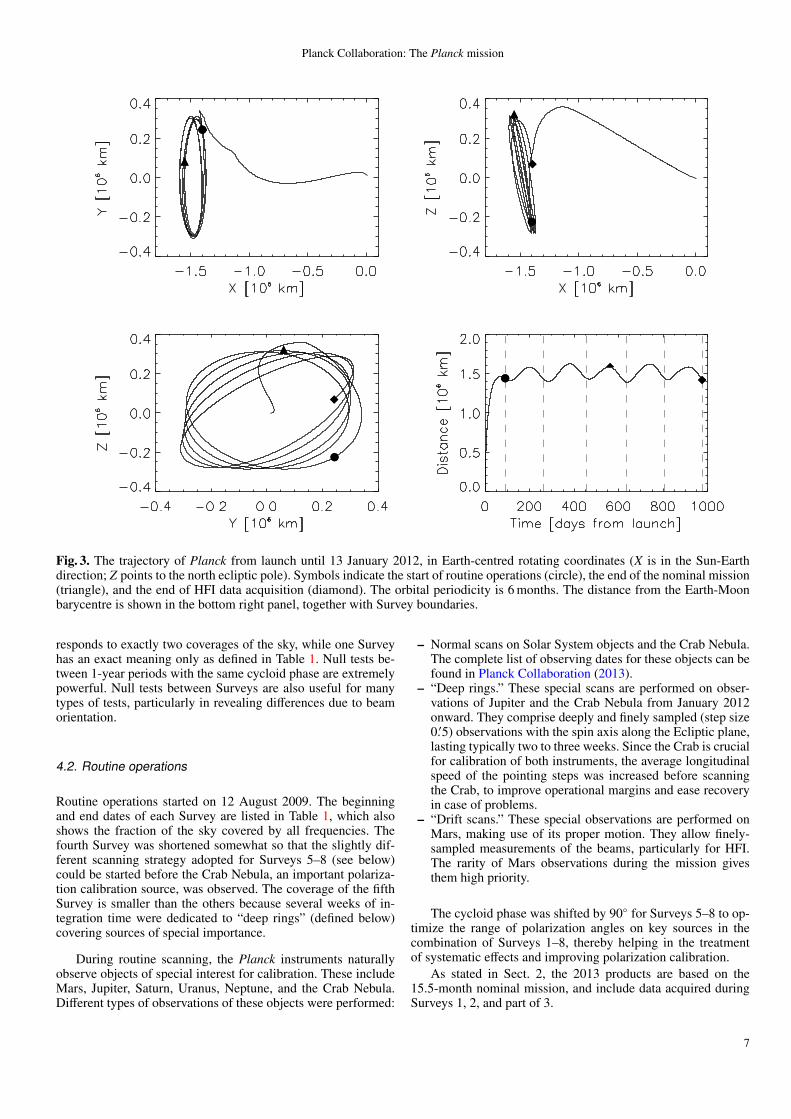
Planck was launched from Kourou, French Guiana, on 14 May2009 on an Ariane 5 ECA rocket, together with the HerschelSpace Observatory. After separation from the rocket and fromHerschel, Planck followed a trajectory to the L2 point of theSun-Earth system. It was injected into a 6-month Lissajous orbitaround L2 in early July 2009 (Fig. 3). Small manoeuvres arerequired at approximately monthly intervals (totalling around1 m s−1 per year) to keep Planck from drifting away from L2.
The first three months of operations focused on commission-ing (during which Planck cooled down to the operating tem-peratures of the coolers and the instruments), calibration, andperformance verification. Routine operations and science obser-vations began 12 August 2009. Detailed information about thefirst phases of operations may be found in Planck CollaborationI (2011) and Planck Collaboration (2013).
4.1. Scanning strategy
Planck spins at 1 rpm about the symmetry axis of the spacecraft.The spin axis follows a cycloidal path across the sky in step-wise displacements of 2′ (Fig. 4). To maintain a steady advanceof the projected position of the spin axis along the ecliptic plane,the time interval between two manoeuvres varies between 2360 sand 3904 s. Details of the scanning strategy are given in Tauberet al. (2010a) and Planck Collaboration I (2011).
The fraction of time used by the manoeuvres themselves(typical duration of five minutes) varies between 6 % and 12 %,depending on the phase of the cycloid. At present, the recon-structed position of the spin axis during manoeuvres has notbeen determined accurately enough for scientific work (but seeSect. 4.5), and the data taken during manoeuvres are not usedin the analysis. Over the nominal mission, the total reduction ofscientific data due to manoeuvres was 9.2 %.
The boresight of the telescope is 85 from the spin axis. AsPlanck spins, the instrument beams cover nearly great circles inthe sky. The spin axis remains fixed (except for a small drift dueto Solar radiation pressure) for between 39 and 65 spins (corre-sponding to the dwell times given above), depending on whichpart of the cycloid Planck is in. To high accuracy, any one beamcovers precisely the same sky between 39 and 65 times. The setof observations made during a period of fixed spin axis point-ing is often referred to as a “ring.” This redundancy plays a keyrole in the analysis of the data, as will be seen below, and is animportant feature of the scan strategy.
As the Earth and Planck orbit the Sun, the nearly-great cir-cles that are observed rotate about the ecliptic poles. The ampli-tude of the spin-axis cycloid is chosen so that all beams of bothinstruments cover the entire sky in one year. In effect, Planck tiltsto cover first one Ecliptic pole, then tilts the other way to coverthe other pole six months later. If the spin axis stayed exactly
5
Planck Collaboration: The Planck mission
HFI ProcessingLFI Processing
LFI Beams & window functs
LFI Calibration
LFI Systematics
HFI Calibration
ComponentSeparation
Overview ofproducts & results
Frequency MapsComponent MapsPower SpectraParameters
Power Spectra& Likelihood
CosmologicalParameters
Catalogue ofcompact sources
Lensing byLSS
Catalogue ofSZ sources
Galactic CO
Consistency ofthe Data
HFI Time Response & Beams
HFI SpectralResponse
HFI Energeticparticle effects
ZodiacalEmission
II
XIII
VI
XXXI
XII
XV
XXVIII
XXIX
XVI
XVII
XIV
X
IX
VII
IV
V
VIII
III
I
Lensing-IRbackgroundcorrelation
XVIII
IntegratedSachs-Wolfe
effectXIX
Cosmology fromSZ counts
XX
Compton para-meter power
spectrumXXi
Constraints oninflation
XXII
Isotropy &statistics of
the CMB
Primordialnon-Gaussianity
XXIII
XXIV
Strings &other defects
XXV
Backgroundgeometry &topology
XXVi
Doppler boost-ing of the
CMBXXVii
All-sky modelof thermal dustXI
CosmicInfrared
BackgroundXXX
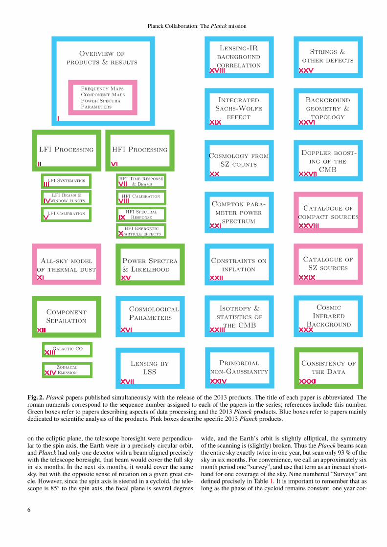
Fig. 2. Planck papers published simultaneously with the release of the 2013 products. The title of each paper is abbreviated. Theroman numerals correspond to the sequence number assigned to each of the papers in the series; references include this number.Green boxes refer to papers describing aspects of data processing and the 2013 Planck products. Blue boxes refer to papers mainlydedicated to scientific analysis of the products. Pink boxes describe specific 2013 Planck products.
on the ecliptic plane, the telescope boresight were perpendicu-lar to the spin axis, the Earth were in a precisely circular orbit,and Planck had only one detector with a beam aligned preciselywith the telescope boresight, that beam would cover the full skyin six months. In the next six months, it would cover the samesky, but with the opposite sense of rotation on a given great cir-cle. However, since the spin axis is steered in a cycloid, the tele-scope is 85 to the spin axis, the focal plane is several degrees
wide, and the Earth’s orbit is slightly elliptical, the symmetryof the scanning is (slightly) broken. Thus the Planck beams scanthe entire sky exactly twice in one year, but scan only 93 % of thesky in six months. For convenience, we call an approximately sixmonth period one “survey”, and use that term as an inexact short-hand for one coverage of the sky. Nine numbered “Surveys” aredefined precisely in Table 1. It is important to remember that aslong as the phase of the cycloid remains constant, one year cor-
6
Planck Collaboration: The Planck mission
Fig. 3. The trajectory of Planck from launch until 13 January 2012, in Earth-centred rotating coordinates (X is in the Sun-Earthdirection; Z points to the north ecliptic pole). Symbols indicate the start of routine operations (circle), the end of the nominal mission(triangle), and the end of HFI data acquisition (diamond). The orbital periodicity is 6 months. The distance from the Earth-Moonbarycentre is shown in the bottom right panel, together with Survey boundaries.
responds to exactly two coverages of the sky, while one Surveyhas an exact meaning only as defined in Table 1. Null tests be-tween 1-year periods with the same cycloid phase are extremelypowerful. Null tests between Surveys are also useful for manytypes of tests, particularly in revealing differences due to beamorientation.
4.2. Routine operations
Routine operations started on 12 August 2009. The beginningand end dates of each Survey are listed in Table 1, which alsoshows the fraction of the sky covered by all frequencies. Thefourth Survey was shortened somewhat so that the slightly dif-ferent scanning strategy adopted for Surveys 5–8 (see below)could be started before the Crab Nebula, an important polariza-tion calibration source, was observed. The coverage of the fifthSurvey is smaller than the others because several weeks of in-tegration time were dedicated to “deep rings” (defined below)covering sources of special importance.
During routine scanning, the Planck instruments naturallyobserve objects of special interest for calibration. These includeMars, Jupiter, Saturn, Uranus, Neptune, and the Crab Nebula.Different types of observations of these objects were performed:
– Normal scans on Solar System objects and the Crab Nebula.The complete list of observing dates for these objects can befound in Planck Collaboration (2013).
– “Deep rings.” These special scans are performed on obser-vations of Jupiter and the Crab Nebula from January 2012onward. They comprise deeply and finely sampled (step size0.′5) observations with the spin axis along the Ecliptic plane,lasting typically two to three weeks. Since the Crab is crucialfor calibration of both instruments, the average longitudinalspeed of the pointing steps was increased before scanningthe Crab, to improve operational margins and ease recoveryin case of problems.
– “Drift scans.” These special observations are performed onMars, making use of its proper motion. They allow finely-sampled measurements of the beams, particularly for HFI.The rarity of Mars observations during the mission givesthem high priority.
The cycloid phase was shifted by 90 for Surveys 5–8 to op-timize the range of polarization angles on key sources in thecombination of Surveys 1–8, thereby helping in the treatmentof systematic effects and improving polarization calibration.
As stated in Sect. 2, the 2013 products are based on the15.5-month nominal mission, and include data acquired duringSurveys 1, 2, and part of 3.
7
Planck Collaboration: The Planck mission
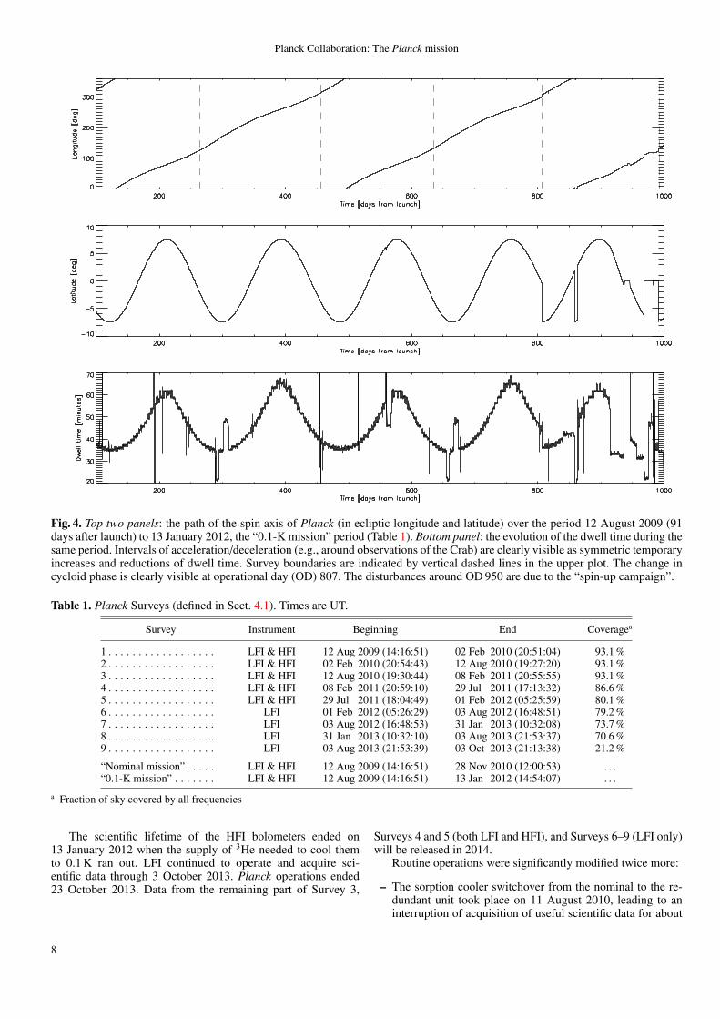
Fig. 4. Top two panels: the path of the spin axis of Planck (in ecliptic longitude and latitude) over the period 12 August 2009 (91days after launch) to 13 January 2012, the “0.1-K mission” period (Table 1). Bottom panel: the evolution of the dwell time during thesame period. Intervals of acceleration/deceleration (e.g., around observations of the Crab) are clearly visible as symmetric temporaryincreases and reductions of dwell time. Survey boundaries are indicated by vertical dashed lines in the upper plot. The change incycloid phase is clearly visible at operational day (OD) 807. The disturbances around OD 950 are due to the “spin-up campaign”.
Table 1. Planck Surveys (defined in Sect. 4.1). Times are UT.
Survey Instrument Beginning End Coveragea
1 . . . . . . . . . . . . . . . . . . LFI & HFI 12 Aug 2009 (14:16:51) 02 Feb 2010 (20:51:04) 93.1 %2 . . . . . . . . . . . . . . . . . . LFI & HFI 02 Feb 2010 (20:54:43) 12 Aug 2010 (19:27:20) 93.1 %3 . . . . . . . . . . . . . . . . . . LFI & HFI 12 Aug 2010 (19:30:44) 08 Feb 2011 (20:55:55) 93.1 %4 . . . . . . . . . . . . . . . . . . LFI & HFI 08 Feb 2011 (20:59:10) 29 Jul 2011 (17:13:32) 86.6 %5 . . . . . . . . . . . . . . . . . . LFI & HFI 29 Jul 2011 (18:04:49) 01 Feb 2012 (05:25:59) 80.1 %6 . . . . . . . . . . . . . . . . . . LFI 01 Feb 2012 (05:26:29) 03 Aug 2012 (16:48:51) 79.2 %7 . . . . . . . . . . . . . . . . . . LFI 03 Aug 2012 (16:48:53) 31 Jan 2013 (10:32:08) 73.7 %8 . . . . . . . . . . . . . . . . . . LFI 31 Jan 2013 (10:32:10) 03 Aug 2013 (21:53:37) 70.6 %9 . . . . . . . . . . . . . . . . . . LFI 03 Aug 2013 (21:53:39) 03 Oct 2013 (21:13:38) 21.2 %
“Nominal mission” . . . . . LFI & HFI 12 Aug 2009 (14:16:51) 28 Nov 2010 (12:00:53) . . .“0.1-K mission” . . . . . . . LFI & HFI 12 Aug 2009 (14:16:51) 13 Jan 2012 (14:54:07) . . .
a Fraction of sky covered by all frequencies
The scientific lifetime of the HFI bolometers ended on13 January 2012 when the supply of 3He needed to cool themto 0.1 K ran out. LFI continued to operate and acquire sci-entific data through 3 October 2013. Planck operations ended23 October 2013. Data from the remaining part of Survey 3,
Surveys 4 and 5 (both LFI and HFI), and Surveys 6–9 (LFI only)will be released in 2014.
Routine operations were significantly modified twice more:
– The sorption cooler switchover from the nominal to the re-dundant unit took place on 11 August 2010, leading to aninterruption of acquisition of useful scientific data for about
8

Planck Collaboration: The Planck mission
two days (one for the operation itself, and one for re-tuningof the cooling chain).
– The satellite’s rotation speed was increased to 1.4 rpm be-tween 8 and 16 December 2011 for observations of Mars,to measure possible systematic effects on the scientific datalinked to the spin rate.
Data were acquired in the normal way during the above twoperiods, but were not used in the 2013 products.
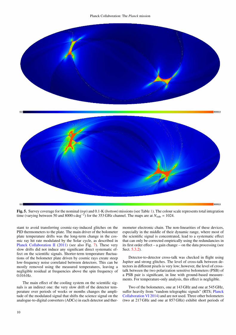
The distribution of integration time over the sky for the nom-inal and “0.1-K” (i.e., until the 3He ran out, see Table 1) mis-sions is illustrated in Fig. 5 for a representative frequency chan-nel. More details can be found in the Explanatory Supplement(Planck Collaboration 2013).
Operations have been extremely smooth throughout the mis-sion. The total observation time lost due to a few anomalies isabout 5 days, spread over the 15.5 months of the nominal mis-sion.
4.3. Satellite environment
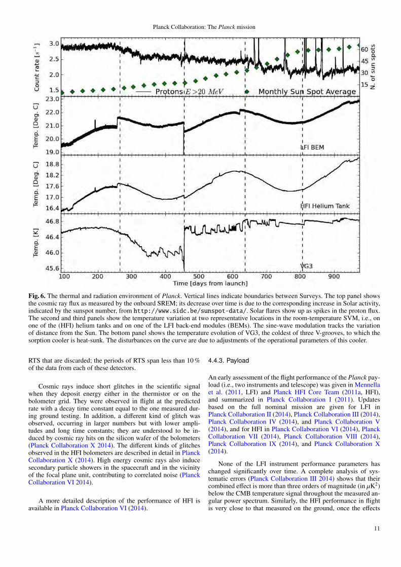
The thermal and radiation environment of the satellite duringthe routine phase is illustrated in Fig. 6. The dominant long-timescale thermal modulation is driven by variations in Solarpower absorbed by the satellite in its elliptical orbit around Sun.The thermal environment is sensitive to various satellite opera-tions. For example, before day 257, the communications trans-mitter was turned on only during the daily data transmissionperiod, causing a daily temperature variation clearly visible atall locations in the Service Module (Fig. 6). Some operationalevents4 had a significant thermal impact as shown in Fig. 6 anddetailed in Planck Collaboration (2013).
The sorption cooler dissipates a large amount of power anddrives temperature variations at multiple levels in the satellite.The bottom panel of Fig. 6 shows the temperature evolution ofthe coldest of the three stacked conical structures or V-groovesthat thermally isolate the warm service module (SVM) from thecold payload module. Most variations of this structure are dueto quasi-weekly power input adjustments of the sorption cooler,whose tube-in-tube heat-exchanger supplying high pressure gasto the 20-K Joule-Thomson valve and returning low pressure gasto the compressor assembly is heat-sunk to it. Many adjustmentsare seen in the roughly three months leading up to switchover.After switchover to the redundant cooler (Sect. 4.4.1), thermalinstabilities were present in the newly operating sorption cooler,which required frequent adjustment, until they reduced signifi-cantly around day 750.
Figure 6 also shows the radiation environment history. AsPlanck started operations, Solar activity was extremely low, andGalactic cosmic rays (which produce sharp “glitches” in the HFIbolometer signals, see Sect. 4.4.2) were more easily able to enterthe heliosphere and hit the satellite. As Solar activity increasedthe cosmic ray flux measured by the onboard standard radiationenvironment monitor (SREM; Planck Collaboration 2013) de-creased correspondingly, but Solar flares increased.
4 Most notably: a) the “catbed” event between 110 and 126 days af-ter launch; b) the “day Planck stood still” 191 days after launch; c) thesorption cooler switchover (OD 460); d) the change in the thermal con-trol loop (OD 540) of the LFI radiometer electronics assembly box; ande) the spin-up campaign around OD 950.
4.4. Instrument environment, operations, and performance
4.4.1. LFI
The front-end of the LFI array is cooled to 20 K by a sorptioncooler system, which included a nominal and a redundant unit(Planck Collaboration II 2011). In early August of 2010, the gas-gap heat switch of one compressor element on the active coolerreached the end of its life. Although the cooler can operate withas few as four (out of six) compressor elements, it was decidedto switch operation to the redundant cooler. On 11 August at17:30 GMT the working cooler was switched off, and the redun-dant one was switched on. Following this operation, an increaseof temperature fluctuations in the 20 K stage was observed. Thecause has been ascribed to the influence of liquid hydrogen re-maining in the cold end of the inactive (previously operating)cooler. These thermal fluctuations produced a measurable effectin the LFI data, but they propagate to the power spectrum at alevel more than four orders of magnitude below the CMB tem-perature signal (Planck Collaboration III 2014) and have a neg-ligible effect on the science data. Furthermore, in February 2011these fluctuations were reduced to a much lower level and haveremained low ever since.
The 22 LFI radiometers have been extremely stable since thebeginning of the observations (Planck Collaboration III 2014),with 1/ f knee frequencies of order 50 mHz and white noise lev-els unchanging within a few percent. After optimization duringthe calibration and performance verification phase, no changesto the bias of the front-end HEMT low-noise amplifiers andphase switches were required throughout the nominal mission.
The main disturbance to LFI data acquisition has been anoccasional bit-flip change in the gain-setting circuit of the dataacquisition electronics, probably due to cosmic ray hits (PlanckCollaboration II 2014). Each of these events leads to the loss ofa fraction of a single ring for the affected detector. The total levelof data loss was extremely low, less than 0.12 % over the wholemission.
4.4.2. HFI
HFI operations were extremely smooth. The instrument param-eters were not changed after being set during the calibration andperformance verification phase.
The satellite thermal environment had no major impact onHFI. A drift of the temperature of the service vehicle module(SVM) due to the eccentricity of the Earth’s orbit (Fig. 6) in-duced negligible changes of temperature of the HFI electronicchain. Induced gain variations are of order 10−4 per degree K.
The HFI dilution cooler (Planck Collaboration II 2011) oper-ated at the lowest available gas flow rate, giving a lifetime twicethe 15.5 months of the nominal mission. This was predicted tobe possible following ground tests, and demonstrates how repre-sentative of the flight environment these difficult tests were.
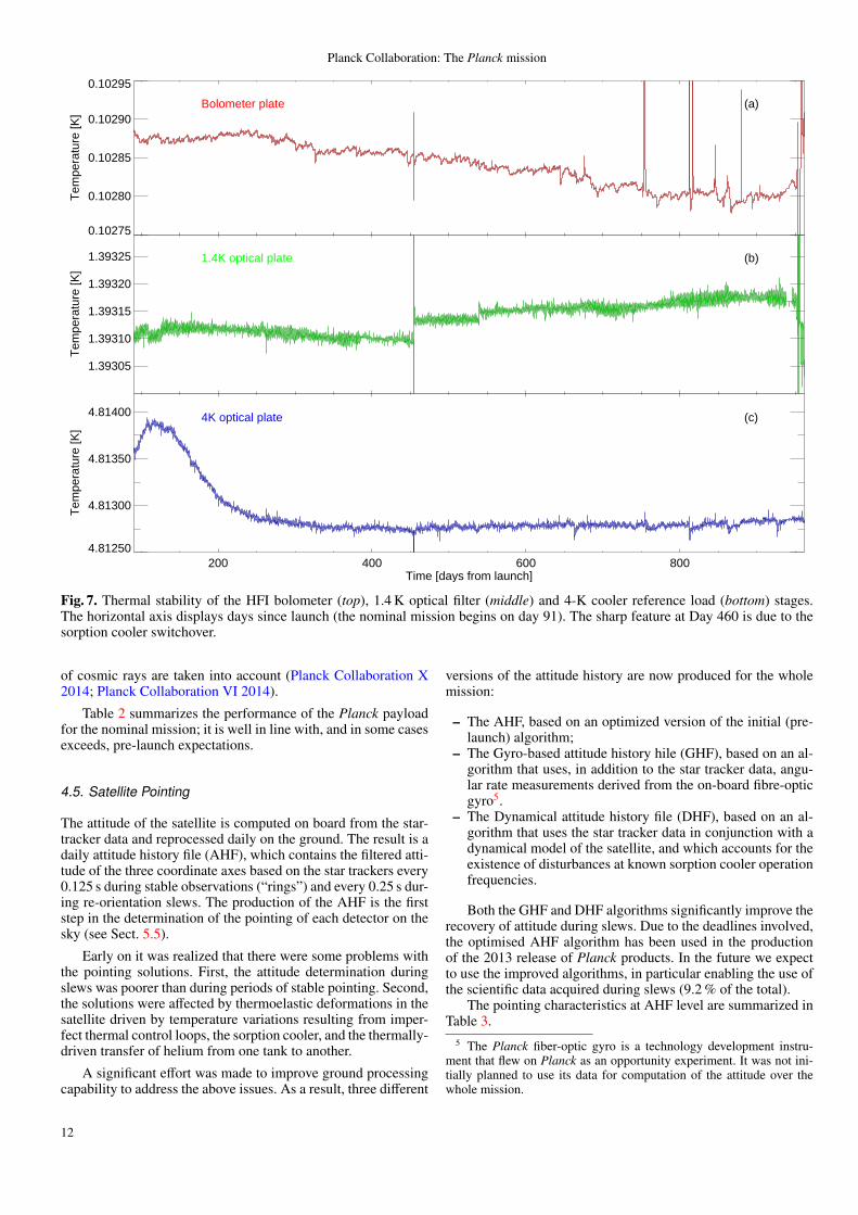
The HFI cryogenic system remained impressively stableover the whole cryogenic mission. Figure 7 shows the temper-ature of the three cold stages of the 4He-JT and dilution cool-ers. The temperature stability of the 1.6 K and 4 K plates, whichsupport the feed horns, couple detectors to the telescope, andsupport the filters, was well within specifications and producednegligible effects on the scientific signals. The dilution coolershowed the secular evolution of heat lift expected from the smalldrifts of the 3He and 4He flows as the pressure in the tanksdecreased. The proportional-integral-differential (PID) temper-ature regulation of the bolometer plate had a long time con-
9
Planck Collaboration: The Planck mission
Fig. 5. Survey coverage for the nominal (top) and 0.1-K (bottom) missions (see Table 1). The colour scale represents total integrationtime (varying between 50 and 8000 s deg−2) for the 353 GHz channel. The maps are at Nside = 1024.
stant to avoid transferring cosmic-ray-induced glitches on thePID thermometers to the plate. The main driver of the bolometerplate temperature drifts was the long-term change in the cos-mic ray hit rate modulated by the Solar cycle, as described inPlanck Collaboration II (2011) (see also Fig. 7). These veryslow drifts did not induce any significant direct systematic ef-fect on the scientific signals. Shorter-term temperature fluctua-tions of the bolometer plate driven by cosmic rays create steeplow-frequency noise correlated between detectors. This can bemostly removed using the measured temperatures, leaving anegligible residual at frequencies above the spin frequency of0.016 Hz.
The main effect of the cooling system on the scientific sig-nals is an indirect one: the very slow drift of the detector tem-perature over periods of weeks or months changes the ampli-tude of the modulated signal that shifts the science signal on theanalogue-to-digital converters (ADCs) in each detector and ther-
mometer electronic chain. The non-linearities of these devices,especially in the middle of their dynamic range, where most ofthe scientific signal is concentrated, lead to a systematic effectthat can only be corrected empirically using the redundancies inits first order effect – a gain change – on the data processing (seeSect. 5.3.2).
Detector-to-detector cross-talk was checked in flight usingJupiter and strong glitches. The level of cross-talk between de-tectors in different pixels is very low; however, the level of cross-talk between the two polarization sensitive bolometers (PSB) ofa PSB pair is significant, in line with ground-based measure-ments. For temperature-only analysis, this effect is negligible.
Two of the bolometers, one at 143 GHz and one at 545 GHz,suffer heavily from “random telegraphic signals” (RTS; PlanckCollaboration VI 2014) and are not used. Three other bolometers(two at 217 GHz and one at 857 GHz) exhibit short periods of
10
Planck Collaboration: The Planck mission
Fig. 6. The thermal and radiation environment of Planck. Vertical lines indicate boundaries between Surveys. The top panel showsthe cosmic ray flux as measured by the onboard SREM; its decrease over time is due to the corresponding increase in Solar activity,indicated by the sunspot number, from http://www.sidc.be/sunspot-data/. Solar flares show up as spikes in the proton flux.The second and third panels show the temperature variation at two representative locations in the room-temperature SVM, i.e., onone of the (HFI) helium tanks and on one of the LFI back-end modules (BEMs). The sine-wave modulation tracks the variationof distance from the Sun. The bottom panel shows the temperature evolution of VG3, the coldest of three V-grooves, to which thesorption cooler is heat-sunk. The disturbances on the curve are due to adjustments of the operational parameters of this cooler.
RTS that are discarded; the periods of RTS span less than 10 %of the data from each of these detectors.
Cosmic rays induce short glitches in the scientific signalwhen they deposit energy either in the thermistor or on thebolometer grid. They were observed in flight at the predictedrate with a decay time constant equal to the one measured dur-ing ground testing. In addition, a different kind of glitch wasobserved, occurring in larger numbers but with lower ampli-tudes and long time constants; they are understood to be in-duced by cosmic ray hits on the silicon wafer of the bolometers(Planck Collaboration X 2014). The different kinds of glitchesobserved in the HFI bolometers are described in detail in PlanckCollaboration X (2014). High energy cosmic rays also inducesecondary particle showers in the spacecraft and in the vicinityof the focal plane unit, contributing to correlated noise (PlanckCollaboration VI 2014).
A more detailed description of the performance of HFI isavailable in Planck Collaboration VI (2014).
4.4.3. Payload
An early assessment of the flight performance of the Planck pay-load (i.e., two instruments and telescope) was given in Mennellaet al. (2011, LFI) and Planck HFI Core Team (2011a, HFI),and summarized in Planck Collaboration I (2011). Updatesbased on the full nominal mission are given for LFI inPlanck Collaboration II (2014), Planck Collaboration III (2014),Planck Collaboration IV (2014), and Planck Collaboration V(2014), and for HFI in Planck Collaboration VI (2014), PlanckCollaboration VII (2014), Planck Collaboration VIII (2014),Planck Collaboration IX (2014), and Planck Collaboration X(2014).
None of the LFI instrument performance parameters haschanged significantly over time. A complete analysis of sys-tematic errors (Planck Collaboration III 2014) shows that theircombined effect is more than three orders of magnitude (in µK2)below the CMB temperature signal throughout the measured an-gular power spectrum. Similarly, the HFI performance in flightis very close to that measured on the ground, once the effects
11
Planck Collaboration: The Planck mission
0.10275
0.10280
0.10285
0.10290
0.10295Te
mpe
ratu
re [K
]
Bolometer plate (a)
1.39305
1.39310
1.39315
1.39320
1.39325
Tem
pera
ture
[K]
1.4K optical plate (b)
200 400 600 800Time [days from launch]
4.81250
4.81300
4.81350
4.81400
Tem
pera
ture
[K]
4K optical plate (c)
Fig. 7. Thermal stability of the HFI bolometer (top), 1.4 K optical filter (middle) and 4-K cooler reference load (bottom) stages.The horizontal axis displays days since launch (the nominal mission begins on day 91). The sharp feature at Day 460 is due to thesorption cooler switchover.
of cosmic rays are taken into account (Planck Collaboration X2014; Planck Collaboration VI 2014).
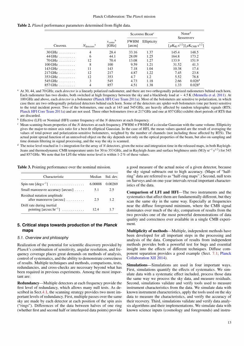
Table 2 summarizes the performance of the Planck payloadfor the nominal mission; it is well in line with, and in some casesexceeds, pre-launch expectations.
4.5. Satellite Pointing
The attitude of the satellite is computed on board from the star-tracker data and reprocessed daily on the ground. The result is adaily attitude history file (AHF), which contains the filtered atti-tude of the three coordinate axes based on the star trackers every0.125 s during stable observations (“rings”) and every 0.25 s dur-ing re-orientation slews. The production of the AHF is the firststep in the determination of the pointing of each detector on thesky (see Sect. 5.5).
Early on it was realized that there were some problems withthe pointing solutions. First, the attitude determination duringslews was poorer than during periods of stable pointing. Second,the solutions were affected by thermoelastic deformations in thesatellite driven by temperature variations resulting from imper-fect thermal control loops, the sorption cooler, and the thermally-driven transfer of helium from one tank to another.
A significant effort was made to improve ground processingcapability to address the above issues. As a result, three different
versions of the attitude history are now produced for the wholemission:
– The AHF, based on an optimized version of the initial (pre-launch) algorithm;
– The Gyro-based attitude history hile (GHF), based on an al-gorithm that uses, in addition to the star tracker data, angu-lar rate measurements derived from the on-board fibre-opticgyro5.
– The Dynamical attitude history file (DHF), based on an al-gorithm that uses the star tracker data in conjunction with adynamical model of the satellite, and which accounts for theexistence of disturbances at known sorption cooler operationfrequencies.
Both the GHF and DHF algorithms significantly improve therecovery of attitude during slews. Due to the deadlines involved,the optimised AHF algorithm has been used in the productionof the 2013 release of Planck products. In the future we expectto use the improved algorithms, in particular enabling the use ofthe scientific data acquired during slews (9.2 % of the total).
The pointing characteristics at AHF level are summarized inTable 3.
5 The Planck fiber-optic gyro is a technology development instru-ment that flew on Planck as an opportunity experiment. It was not ini-tially planned to use its data for computation of the attitude over thewhole mission.
12
Planck Collaboration: The Planck mission
Table 2. Planck performance parameters determined from flight data.
Scanning Beamc NoisedSensitivity
νcenterb FWHM Ellipticity
Channel Ndetectorsa [GHz] [arcm] [ µKRJ s1/2] [ µKCMB s1/2]
30 GHz . . . . . . . . 4 28.4 33.16 1.37 145.4 148.544 GHz . . . . . . . . 6 44.1 28.09 1.25 164.8 173.270 GHz . . . . . . . . 12 70.4 13.08 1.27 133.9 151.9
100 GHz . . . . . . . . 8 100 9.59 1.21 31.52 41.3143 GHz . . . . . . . . 11 143 7.18 1.04 10.38 17.4217 GHz . . . . . . . . 12 217 4.87 1.22 7.45 23.8353 GHz . . . . . . . . 12 353 4.7 1.2 5.52 78.8545 GHz . . . . . . . . 3 545 4.73 1.18 2.66 0.026d
857 GHz . . . . . . . . 4 857 4.51 1.38 1.33 0.028d
a At 30, 44, and 70 GHz, each detector is a linearly polarized radiometer, and there are two orthogonally polarized radiometers behind each horn.Each radiometer has two diodes, both switched at high frequency between the sky and a blackbody load at ∼ 4.5 K (Mennella et al. 2011). At100 GHz and above, each detector is a bolometer (Planck HFI Core Team 2011a). Most of the bolometers are sensitive to polarization, in whichcase there are two orthogonally polarized detectors behind each horn. Some of the detectors are spider-web bolometers (one per horn) sensitiveto the total incident power. Two of the bolometers, one each at 143 and 545 GHz, are heavily affected by random telegraphic signals (RTS;Planck HFI Core Team 2011a) and are not used. Three other bolometers (two at 217 GHz and one at 857 GHz) exhibit short periods of RTS thatare discarded.
b Effective (LFI) or Nominal (HFI) center frequency of the N detectors at each frequency.c Mean scanning-beam properties of the N detectors at each frequency. FWHM ≡ FWHM of a circular Gaussian with the same volume. Ellipticity
gives the major-to-minor axis ratio for a best-fit elliptical Gaussian. In the case of HFI, the mean values quoted are the result of averaging thevalues of total-power and polarization-sensitive bolometers, weighted by the number of channels (not including those affected by RTS). Theactual point spread function of an unresolved object on the sky depends not only on the optical properties of the beam, but also on sampling andtime domain filtering in signal processing, and the way the sky is scanned.
d The noise level reached in 1 s integration for the array of N detectors, given the noise and integration time in the released maps, in both Rayleigh-Jeans and thermodynamic CMB temperature units for 30 to 353 GHz, and in Rayleigh-Jeans and surface brightness units (M Jy sr−1 s1/2) for 545and 857 GHz. We note that for LFI the white noise level is within 1-2 % of these values.
Table 3. Pointing performance over the nominal mission.
Characteristic Median Std. dev.
Spin rate [deg s−1] . . . . . . . . . . . . . . . . . 6.00008 0.00269
Small manoeuvre accuracy [arcsec] . . . . . 5.1 2.5
Residual nutation amplitudeafter manoeuvre [arcsec] . . . . . . . . . 2.5 1.2
Drift rate during inertialpointing [arcsec hr−1] . . . . . . . . . . . 12.4 1.7
5. Critical steps towards production of the Planckmaps
5.1. Overview and philosophy
Realization of the potential for scientific discovery provided byPlanck’s combination of sensitivity, angular resolution, and fre-quency coverage places great demands on methods of analysis,control of systematics, and the ability to demonstrate correctnessof results. Multiple techniques and methods, comparisons, tests,redundancies, and cross-checks are necessary beyond what hasbeen required in previous experiments. Among the most impor-tant are:
Redundancy—Multiple detectors at each frequency provide thefirst level of redundancy, which allows many null tests. As de-scribed in Sect.4.1, the scanning strategy provides two more im-portant levels of redundancy. First, multiple passes over the samesky are made by each detector at each position of the spin axis(“rings”). Differences of the data between halves of one ring(whether first and second half or interleaved data points) provide
a good measure of the actual noise of a given detector, becausethe sky signal subtracts out to high accuracy. (Maps of “half-ring” data are referred to as “half-ring maps”.) Second, null testson Surveys and on one-year intervals reveal important character-istics of the data.
Comparison of LFI and HFI—The two instruments and thesystematics that affect them are fundamentally different, but theyscan the same sky in the same way. Especially at frequenciesnear the diffuse foreground minimum, where the CMB signaldominates over much of the sky, comparison of results from thetwo provides one of the most powerful demonstrations of dataquality and correctness ever available in a single CMB experi-ment.
Multiplicity of methods—Multiple, independent methods havebeen developed for all important steps in the processing andanalysis of the data. Comparison of results from independentmethods provides both a powerful test for bugs and essentialinsight into the effects of different techniques. Diffuse com-ponent separation provides a good example (Sect. 7.1; PlanckCollaboration XII 2014).
Simulations—Simulations are used in four important ways.First, simulations quantify the effects of systematics. We sim-ulate data with a systematic effect included, process those datathe same way we process the sky data, and measure residuals.Second, simulations validate and verify tools used to measureinstrument characteristics from the data. We simulate data withknown instrument characteristics, apply the tools used on the skydata to measure the characteristics, and verify the accuracy oftheir recovery. Third, simulations validate and verify data analy-sis algorithms and their implementations. We simulate data withknown science inputs (cosmology and foregrounds) and instru-
13
Planck Collaboration: The Planck mission
ment characteristics (beams, bandpasses, noise), apply the anal-ysis tools used on the sky data, and verify the accuracy of re-covered inputs. Fourth, simulations support analysis of the skydata. We generate massive Monte Carlo simulation sets of theCMB and noise, and pass them through the analyses used on thesky data to quantify uncertainties and correct biases. The firsttwo uses are instrument-specific; distinct pipelines have beendeveloped and employed by LFI and HFI. The last two usesrequire consistent simulations of both instruments in tandem.Furthermore, the Monte Carlo simulation-sets are the most com-putationally intensive part of the Planck data analysis and re-quire large computational capacity and capability.
5.2. Simulations
We simulate time-ordered information (TOI) for the full focalplane (FFP) for the nominal mission. Each FFP simulation com-prises a single “fiducial” realization (CMB, astrophysical fore-grounds, and noise), together with separate Monte Carlo (MC)realizations of the CMB and noise. The first Planck cosmologyresults were supported primarily by the sixth FFP simulation-set,hereafter FFP6. The first five FFP realizations were less compre-hensive and were primarily used for validation and verificationof the Planck analysis codes and for cross-validation of the DataProcessing Centres (DPCs) and FFP simulation pipelines.
To mimic the sky data as closely as possible, FFP6 usedthe actual pointing, data flags, detector bandpasses, beams, andnoise properties of the nominal mission. For the fiducial real-ization, maps were made of the total observation (CMB, fore-grounds, and noise) at each frequency for the nominal missionperiod, using the Planck Sky Model (Delabrouille et al. 2012).In addition, maps were made of each component separately, ofsubsets of detectors at each frequency, and of half-ring and sin-gle Survey subsets of the data. The noise and CMB Monte Carlorealization-sets also included both all and subsets of detectors ateach frequency, and full and half-ring data sets for each detectorcombination. With about 125 maps per realization and 1000 re-alizations of both the noise and CMB, FFP6 totals some 250,000maps — by far the largest simulation set ever fielded in supportof a CMB mission.
5.3. Timeline processing
5.3.1. LFI
The processing of LFI data (Planck Collaboration II–V 2013)is divided into three levels. Level 1 retrieves information fromtelemetry packets and auxiliary data received each day from theMission Operation Center (MOC), and transforms the scientifictime-ordered information (TOI) and housekeeping (H/K) datainto a form that is manageable by the Level 2 scientific pipeline.
The Level 1 steps are:
– uncompress the retrieved packets;– de-quantize and de-mix the uncompressed packets to retrieve
the original signal in analogue-to-digital units (ADU);– transform ADU data into volts; and– time stamp each sample.
The Level 1 software has not changed since the start of the mis-sion. Detailed information is given in Zacchei et al. (2011) andPlanck Collaboration II (2014).
Level 2 processes scientific and H/K information into dataproducts. The highly stable behaviour of the LFI radiometers
means that very few corrections are required in the data process-ing at either TOI or map level. The main Level 2 steps are:
– Build the reduced instrument model (RIMO) that containsall the main instrumental characteristics (beam size, spectralresponse, white noise etc).
– Remove spurious effects at the diode level. Small electricaldisturbances, synchronous with the 1-Hz on-board clock, areremoved from the 44 GHz data streams. For some channels(in particular LFI25M-01) non-linear behaviour of the ADCis corrected by analyzing the white noise level of the totalpower component. No corrections are applied to compensatefor thermal fluctuations in the 4 K, 20 K, and 300 K stages ofthe instrument, since H/K monitoring and instrument thermalmodelling confirm that their effect is below significance.
– Compute and apply the gain modulation factor to minimizethe 1/ f noise. The LFI timelines are produced by taking dif-ferences between the signals from the sky and from internalblackbody reference loads cooled to about 4.5 K. Radiometerbalance is optimized by introducing a gain modulation fac-tor, typically stable to 0.04 % throughout the mission, whichgreatly reduces 1/ f noise and improves immunity from awide class of systematic effects.
– Combine the diodes to remove a small anti-correlated com-ponent in the white noise.
– Identify and flag periods of time containing anomalous fluc-tuations in the signal. Fewer than 1 % of the data acquiredduring the nominal mission are flagged.
– Compute the corresponding detector pointing for each sam-ple based on auxiliary data and the reconstructed focal planegeometry (Sect. 5.5).
– Calibrate the scientific timelines in physical units (KCMB),fitting the dipole convolved with a 4π representation of thebeam (Sect. 5.6).
– Combine the calibrated TOIs into maps at each frequency(Sect. 6.2.1).
Level 3 then collects instrument-specific Level 2 outputs(from both HFI and LFI) and derives various scientific productsas maps of separated astrophysical components.
5.3.2. HFI
Following Level 1 processing similar to that of LFI, the HFI datapipeline consists of TOI processing, followed by map makingand calibration (Planck Collaboration VI–X 2013).
The HFI processing pipeline steps are:
– Demodulate, as required by the AC square-wave polarizationbias of the bolometers.
– Flag and remove cosmic-ray-induced glitches, including thelong-time-constant tails of glitches induced in the siliconwafer. More than 95 % of the acquired samples are affectedby glitches. Glitch templates constructed from averages arefitted and subtracted from the timelines; the fast part of eachglitch is rejected. The fraction of time-ordered data rejecteddue to glitches is 16.5 %6 when averaged over the nominalmission.
– Correct for the slow drift of the bolometer response inducedby the bolometer plate temperature variation described inSect. 4.4.2. A baseline drift estimated from the signal fromthe dark bolometers on the same plate (smoothed over 60 s)is removed from each timeline.
6 varying from 10 to 26.7 % depending on the bolometer.
14
Planck Collaboration: The Planck mission
– Deconvolve the bolometer complex time response (analyzedin detail in Planck Collaboration VII (2014)).
– Remove the narrow lines induced by electromagnetic inter-ference from the 4He-JT cooler, exploiting the fact that thecooler is synchronized with the HFI readout and operates ata harmonic of the sampling rate.
– Analyze the statistics of the time-scale of pointing periodsand discard anomalous ones (less than 1 % of the data arediscarded).
Apparent gain variations seen when comparing identicalpointing circles one year apart actually originate in non-linearities in the ADCs of the bolometer readout system.Lengthy on-board measurements of the non-linear properties ofthe ADCs have been carried after the end of 0.1-K operations,and algorithms to correct for these non-linearities have beendeveloped. The electromagnetic interference from the 4He-JTcooler described above induces voltages in the readout circuitsbefore digitization by the ADC. That interference itself is lo-calized in frequency and therefore easy to remove; however, itmakes it more difficult to estimate the ADC non-linearity cor-rection accurately for the detectors most affected by it. The ADCnon-linearity correction is still under development and has notbeen applied to the data in this 2013 release. Instead, a calibra-tion scheme (see Sect. 5.6 and Planck Collaboration VIII 2014)that estimates a varying gain corrects very well the first ordereffects of the ADC non-linearity. A full correction will be im-plemented for the release in 2014 of the polarization data, forwhich higher order effects are not negligible.
5.4. Beams
As described in Planck Collaboration IV (2014), the main beamparameters of the LFI detectors and the geometry of the focalplane were determined using Jupiter as a source. By combiningfour Jupiter transits (around days 170, 415, 578, and 812) thebeam shapes were measured down to −20 dB from peak at 30and 44 GHz, and −25 dB at 70 GHz. The FWHM of the beams isdetermined with a typical uncertainty of 0.3 % at 30 and 44 GHz,and 0.2 % at 70 GHz. The alignment of the focal plane and the lo-cation of each detector’s phase centre were determined by vary-ing their values in a GRASP7 physical optics model to minimizethe difference between model co-polar and cross-polar patternsand the measurements. To estimate the uncertainties in the de-termination of the in-flight beam models, a set of optical modelsrepresentative of the measured LFI scanning beams7 was found,using GRASP to randomly distort the wavefront error of thephysical model of telescope and detectors, then rejecting thosedistorted models whose predicted patterns fell outside the errorenvelope of the measured ones.
Sidelobe pick-up by the LFI of the CMB dipole and diffuseGalactic emission (Planck Collaboration III 2014) is clearly seenat the ∼ 10 µK level in odd-even Survey difference maps (whichenhance the effects of sidelobes) at 30 GHz. This contaminationwas fitted to a model that incorporates the radiometer bandpassand the optical response variation across the band. The modelledcontamination was then removed. Residual straylight effects inthe maps are estimated to be less than ∼ 2 µK at all frequencies.
The in-flight scanning beams8 of HFI (Planck CollaborationVII 2014) were measured using observations of Mars.
7 developed by TICRA, http://www.ticra.com/8 The term “scanning beam” refers to the angular response of a sin-
gle detector to a compact source, including the optical beam and (forHFI) the effects of time domain filtering. In the case of HFI, a Fourier
Observations of Saturn and Jupiter are used to estimate the nearsidelobes and other residuals. The HFI bolometers have a com-plex time response, characterized by multiple time constants. Toobtain a compact scanning beam, this time behaviour must bedeconvolved from the measured timelines. The deconvolutionalgorithm is iterative, allowing an estimate of the parameters ofthe bolometer transfer function, and forcing the resulting scan-ning beams to be more compact. A spline representation of thebeams is used, allowing capture of the near-sidelobe structuredown to about -40 dB from the peak. Stacking of multiple cross-ings of Saturn and Jupiter allows us to obtain high SNR maps ofthese near sidelobes, and to quantify the level of unmodelled ef-fects. The stacked data at 353 GHz show the presence of skirts inthe pattern close to the main beam due to diffraction at the edgeof the secondary mirror. These skirts could not be measured ac-curately at lower frequencies with the 2013 data and were notincluded in the beam representation (Section 6.1). Instead, up-per limits to their contribution to the solid angle at each fre-quency were estimated (Planck Collaboration VII 2014) to bein the range 0.2 to 0.4 %, and were included in the uncertaintybudget for the gain calibration and transfer functions.
At the three highest frequencies, the stacked planet maps alsoclearly reveal sharp “grating lobes” due to dimpling of the tele-scope reflector surfaces into the cells of the internal honeycombstructure (Tauber et al. 2010b). The amplitude of these lobes islarger than predicted, possibly indicating mechanical changes inthe reflectors after launch; however, the total power contained inthese lobes remains negligible in terms of impact on the scien-tific data, and therefore they are ignored in the scanning beammodel.
The uncertainties in the estimation of the HFI scanningbeams and other systematic effects in the maps are determined atwindow function level, using realistic Monte-Carlo simulationsthat include pointing effects, detector noise, and measurementeffects. Additional estimates are made of the effect of planetemission variability, beam colour corrections, and more. Thetotal uncertainties in the scanning beam solid angles are under0.5 % for the CMB channels.
Sidelobe pick-up by the HFI due to spillover past the primaryreflector (Tauber et al. 2010b), is clearly seen in Survey differ-ence maps at 545 and 857 GHz (Planck Collaboration XIV 2014)at times when the central part of the Galactic plane is alignedwith the elongated far sidelobe. GRASP models are fit to odd-even Survey difference maps to estimate sidelobe levels for eachdetector. These levels are highly variable between the 857 GHzdetectors and not in agreement with levels predicted by GRASP;this difference may plausibly be caused by deviations of the as-built horns from the design. A model of the primary reflectorspillover signal can then be removed from the time-ordered databefore mapmaking. Being close to the spin axis, these signalsare largely unmodulated by the spinning motion, and are mostlyremoved by the destriping map-making code (this is the case forboth instruments).
The HFI far sidelobe signals and zodiacal light can be re-moved at TOI level in the same pipeline. Two sets of maps arereleased in 2013 Planck Collaboration VI (2014). In the “de-fault” set, far sidelobes and zodiacal light are not removed. Inthe second set, far sidelobes and zodiacal light are removed.
filter deconvolves the bolometer/electronics time response and lowpass-filters the data. In the case of LFI, the sampling tends to smear signal inthe time domain.
15
Planck Collaboration: The Planck mission
5.5. Focal Plane Geometry and Pointing
The focal plane geometry9 of LFI was determined independentlyfor each Jupiter crossing (Planck Collaboration IV 2014). Thesolutions for the first and second and for the third and fourthcrossings agree to 2′′; however, a shift of ∼15 arcsecs (largelyin the in-scan direction) is found between the two pairs. For thisreason, the focal plane geometry is assumed constant over time,with the exception of a single jump on day 540.
The focal plane geometry of the HFI detectors was also mea-sured using planet observations (Planck Collaboration VI 2014;Planck Collaboration VII 2014). The relative location of individ-ual detectors differs from the ground prediction typically by 1′,mainly in the in-scan direction, indicating some de-alignment ofthe HFI focal plane or of the telescope in flight. The high SNRavailable on Jupiter allows us to estimate pointing “errors” ona 1-minute timescale; these measurements show the presence ofthermo-elastic deformations of the star tracker mounting struc-ture that are well correlated with a known on-board thermal con-trol cycle. This specific cycle was changed on OD 540, leadingto a reduction in this “error” from 3′′ to 1′′. These small high-frequency effects are not taken into account at the present time;however, larger (up to 15′′) slow pointing variations are observedwith time scales of order 100 days using measurements of brightcompact radio sources. The HFI focal plane geometry variationwith time is corrected for this trend, leaving an estimated totalpointing reconstruction error of a few arcseconds rms.
The time-dependent pointing direction of each detector inPlanck is based on the filtered star tracker data provided in thedaily Attitude History Files (see Sect. 4.5), corrected for threeeffects: 1) changes in the inertial tensor of the satellite resultingfrom fluid depletion; 2) time-varying thermoelastic deformationsof the structure between the star tracker and the telescope bore-sight; and 3) stellar aberration. The measured focal plane geom-etry is then used to estimate the corrected pointing timestreamfor each detector.
Time-stamping of all detector samples is synchronized to thesatellite’s Central Time Reference, also used by the star trackers.The stability of this reference has been shown to have negligibleimpact on Planck’s science products, when compared to othersources (Planck Collaboration 2013).
5.6. Calibration
The photometric (gain) calibrations of LFI and HFI are achievedby comparing the measured data against the expected signalfrom the Solar and orbital dipoles. The Solar dipole parametersare assumed to be those determined by WMAP7 (Jarosik et al.2011), which during the initial period of Planck analysis pro-vided a convenient, stable, and accurate reference. In the future,a Planck-determined dipole will replace the WMAP7 dipole.The orbital dipole is determined from the measured satellite or-bital motion, so in principle it can provide an independent abso-lute calibration.
In the LFI pipeline (Planck Collaboration V 2014), a full 4πbeam is used to calculate the expected dipole signal. An iterativefit outside a Galactic mask plus low-frequency filtering yields asingle calibration constant for each pointing period (or ring). For44 and 70 GHz, an adaptive smoothing function removes the ef-fect of low-frequency noise stripes from the time series of ringgains. The 30 GHz data are more affected by sidelobe signals;for this channel it has been found more effective to estimate the
9 That is, the relative location on the sky of the multiple detectors.
relative changes in the ring gains over time by using the totalpower variations of the 4-K reference loads measured by each ra-diometer. This relative estimation is carried out over three differ-ent time periods (to account for significant temperature changesin the 20 K and 4 K stages due to operational events). The esti-mated gains are applied to the acquired data in the time domain.The Solar and orbital dipole signals are then removed from thetime-ordered data before proceeding into mapmaking.
At the present stage, the overall uncertainty in the LFI cal-ibration relative to the WMAP Solar dipole is of order 0.4 %,dominated by the beam uncertainty over the band (0.1–0.4 %depending on the frequency), sidelobe convolution (∼ 0.2 %),and residual systematics (0.1–0.2 %). There is a 0.25 % uncer-tainty in the WMAP dipole itself (Hinshaw et al. 2009), which weconservatively add linearly to the LFI relative calibration uncer-tainty to get the overall calibration uncertainties given in Table6.
Preliminary results on the orbital dipole as measured by LFIare in agreement with WMAP at around the 1σ level. This indi-cates good consistency of LFI and WMAP calibrations at ` = 1.The inter-channel calibration discussed below allows us to ex-trapolate the independent measurement of the Solar dipole bythe LFI to the HFI CMB channels.
In the HFI pipeline (Planck Collaboration VIII 2014), a pen-cil beam is assumed when comparing data to the expected dipolesignal. In this process, the contribution of the far sidelobes dueto spillover past the primary reflector (see Sect. 5.4) is neglected.Its contribution to the Solar dipole signal is estimated to be∼0.13 % after destriping, and affects only large angular scales(` < 10). Near-side-lobe corrections are more substantial (0.2–0.4 %, see Sect. 5.4) but have not yet been implemented. Theseeffects are small compared to other corrections not yet made,such as the ADC non-linearity for HFI (see Sect. 5.3.2) or beamuncertainties over the band for LFI (Planck Collaboration V2014).
Fitting for the HFI gains is done at ring level, including aspatial model of Galactic emission based on HFI maps, but ex-cluding the Galactic plane. It yields three parameters per ring:a dipole gain, a Galactic gain, and an offset. An initial gainmodel consists of a fixed gain averaged over a contiguous setof 4000 rings, where the ring-to-ring dispersion is less than 1 %.An iterative scheme is then applied to the 100–217 GHz chan-nels that fits for relative variations of the gain over the wholemission. This scheme is not applied to the 353 GHz channel be-cause intra-pixel emission gradients cause instability in the iter-ations. Remaining residuals in the calibrated rings are estimatedby comparisons between detectors, and are of order 0.3 % for100–217 GHz and 1 % at 353 GHz. Once the HFI rings are cali-brated, they are converted to maps using a destriping algorithm(see Sect. 6.2.2), and the WMAP7 dipole is removed from themaps.
The current calibration scheme of HFI has been checkedagainst an independent algorithm based only on the orbitaldipole (Tristram et al. 2011). Relative variations are typically0.1 % and always smaller than 0.2 % except for a systematicbias of 0.5–1 % believed to be due to the (currently uncorrected)ADC non-linearities (Sect. 5.3.2), which affect the two methodsdifferently. The total gain calibration accuracy, as evaluated fromthe ring-to-ring variability, overestimates the real accuracy sincepart of the variability is being corrected.
Calibrated maps can be examined for signatures of calibra-tion errors. The presence of Solar dipole residuals provides lim-its to the quality of the LFI and HFI calibration processes withrespect to their common reference, i.e., the WMAP Solar dipole.
16
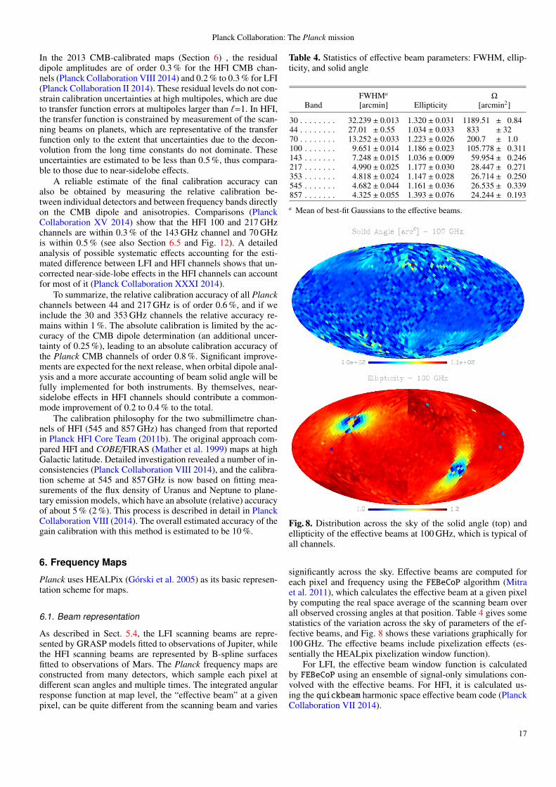
Planck Collaboration: The Planck mission
In the 2013 CMB-calibrated maps (Section 6) , the residualdipole amplitudes are of order 0.3 % for the HFI CMB chan-nels (Planck Collaboration VIII 2014) and 0.2 % to 0.3 % for LFI(Planck Collaboration II 2014). These residual levels do not con-strain calibration uncertainties at high multipoles, which are dueto transfer function errors at multipoles larger than `=1. In HFI,the transfer function is constrained by measurement of the scan-ning beams on planets, which are representative of the transferfunction only to the extent that uncertainties due to the decon-volution from the long time constants do not dominate. Theseuncertainties are estimated to be less than 0.5 %, thus compara-ble to those due to near-sidelobe effects.
A reliable estimate of the final calibration accuracy canalso be obtained by measuring the relative calibration be-tween individual detectors and between frequency bands directlyon the CMB dipole and anisotropies. Comparisons (PlanckCollaboration XV 2014) show that the HFI 100 and 217 GHzchannels are within 0.3 % of the 143 GHz channel and 70 GHzis within 0.5 % (see also Section 6.5 and Fig. 12). A detailedanalysis of possible systematic effects accounting for the esti-mated difference between LFI and HFI channels shows that un-corrected near-side-lobe effects in the HFI channels can accountfor most of it (Planck Collaboration XXXI 2014).
To summarize, the relative calibration accuracy of all Planckchannels between 44 and 217 GHz is of order 0.6 %, and if weinclude the 30 and 353 GHz channels the relative accuracy re-mains within 1 %. The absolute calibration is limited by the ac-curacy of the CMB dipole determination (an additional uncer-tainty of 0.25 %), leading to an absolute calibration accuracy ofthe Planck CMB channels of order 0.8 %. Significant improve-ments are expected for the next release, when orbital dipole anal-ysis and a more accurate accounting of beam solid angle will befully implemented for both instruments. By themselves, near-sidelobe effects in HFI channels should contribute a common-mode improvement of 0.2 to 0.4 % to the total.
The calibration philosophy for the two submillimetre chan-nels of HFI (545 and 857 GHz) has changed from that reportedin Planck HFI Core Team (2011b). The original approach com-pared HFI and COBE/FIRAS (Mather et al. 1999) maps at highGalactic latitude. Detailed investigation revealed a number of in-consistencies (Planck Collaboration VIII 2014), and the calibra-tion scheme at 545 and 857 GHz is now based on fitting mea-surements of the flux density of Uranus and Neptune to plane-tary emission models, which have an absolute (relative) accuracyof about 5 % (2 %). This process is described in detail in PlanckCollaboration VIII (2014). The overall estimated accuracy of thegain calibration with this method is estimated to be 10 %.
6. Frequency Maps
Planck uses HEALPix (Gorski et al. 2005) as its basic represen-tation scheme for maps.
6.1. Beam representation
As described in Sect. 5.4, the LFI scanning beams are repre-sented by GRASP models fitted to observations of Jupiter, whilethe HFI scanning beams are represented by B-spline surfacesfitted to observations of Mars. The Planck frequency maps areconstructed from many detectors, which sample each pixel atdifferent scan angles and multiple times. The integrated angularresponse function at map level, the “effective beam” at a givenpixel, can be quite different from the scanning beam and varies
Table 4. Statistics of effective beam parameters: FWHM, ellip-ticity, and solid angle
FWHMa ΩBand [arcmin] Ellipticity [arcmin2]
30 . . . . . . . . 32.239 ± 0.013 1.320 ± 0.031 1189.51 ± 0.8444 . . . . . . . . 27.01 ± 0.55 1.034 ± 0.033 833 ± 3270 . . . . . . . . 13.252 ± 0.033 1.223 ± 0.026 200.7 ± 1.0100 . . . . . . . 9.651 ± 0.014 1.186 ± 0.023 105.778 ± 0.311143 . . . . . . . 7.248 ± 0.015 1.036 ± 0.009 59.954 ± 0.246217 . . . . . . . 4.990 ± 0.025 1.177 ± 0.030 28.447 ± 0.271353 . . . . . . . 4.818 ± 0.024 1.147 ± 0.028 26.714 ± 0.250545 . . . . . . . 4.682 ± 0.044 1.161 ± 0.036 26.535 ± 0.339857 . . . . . . . 4.325 ± 0.055 1.393 ± 0.076 24.244 ± 0.193a Mean of best-fit Gaussians to the effective beams.
Fig. 8. Distribution across the sky of the solid angle (top) andellipticity of the effective beams at 100 GHz, which is typical ofall channels.
significantly across the sky. Effective beams are computed foreach pixel and frequency using the FEBeCoP algorithm (Mitraet al. 2011), which calculates the effective beam at a given pixelby computing the real space average of the scanning beam overall observed crossing angles at that position. Table 4 gives somestatistics of the variation across the sky of parameters of the ef-fective beams, and Fig. 8 shows these variations graphically for100 GHz. The effective beams include pixelization effects (es-sentially the HEALpix pixelization window function).
For LFI, the effective beam window function is calculatedby FEBeCoP using an ensemble of signal-only simulations con-volved with the effective beams. For HFI, it is calculated us-ing the quickbeam harmonic space effective beam code (PlanckCollaboration VII 2014).
17
Planck Collaboration: The Planck mission
To estimate the uncertainties of the effective beams, the en-semble of allowed LFI GRASP models (Sect. 5.4) is propagatedthrough FEBeCoP. For HFI, quickbeam is used to propagate anensemble of simulated Mars observations to harmonic space.The total uncertainties in the effective beam window function(in B2
` units) at ` = 600 are 2 % at 30 GHz and 1.5 % at 44 GHz.At ` = 100, they are 0.7 %, 0.5 %, 0.2 %, and 0.2 % for 70, 100,143, and 217 GHz respectively (Planck Collaboration IV 2014;Planck Collaboration VII 2014).
6.2. Mapmaking
6.2.1. LFI
Maps of the LFI channels are made using the Madam destripingcode (Keihanen et al. 2010), from calibrated TOI of each ra-diometer and the corresponding pointing data in the form of theEuler angles (θ, φ, ψ). Madam is a polarized, maximum-likelihoodcode. The noise is modelled as white noise plus a set of offsets,or baselines. The algorithm estimates the amplitudes of the base-lines, subtracts them from the TOI, and bins the result into mapsof the Stokes parameters T , Q, and U. The resulting T maps areshown in Fig. 9.
A key parameter in the Madam algorithm is the baselinelength, the time interval over which the baseline approximationto low-frequency noise is applied. We choose baseline lengthscorresponding to an integer number of samples (33, 47, and 79 at30, 44, and 70 GHz, respectively) such that the total integrationtime over the baseline corresponds approximately to one second.This selection is based on a compromise between computationalload and map quality, and we find that shortening the baselinesbelow one second has practically no effect on the residual noise.Madam requires an estimate of the noise covariance matrix.
In general, we use a white noise covariance matrix. The pipelineallows the use of different user-defined weighting schemes. Themaps being released are made using the horn-uniform weightingscheme with
C−1w =
2σ2
M + σ2S
, (1)
where σM and σS are the white noise levels of the Main and Sideradiometers of a given horn, weighted equally.
Half-ring maps (Sect. 5.1) are made in the same way. A time-weighted difference between the first-half and second-half ringmaps captures the noise properties directly from the data of noisecomponents whose frequency is f >∼ 2/20 min = 1.7 mHz, i.e.,half the duration of the pointing period.
The monopoles in Planck maps are unconstrained, and itis conventional to adjust them such that they yield plausiblevalues of the diffuse Galactic foreground signals. For LFI, themonopoles are estimated (Planck Collaboration V 2014) in a1-diameter patch at high galactic latitudes, first subtracting theCMB (using the independent component analysis estimate de-scribed in Sec. 7.1), and then carrying out a multi-frequencyforeground fit using both Planck and WMAP channels. The off-sets in each map are then adjusted to attain the fitted foregroundlevel.
6.2.2. HFI
Maps of the HFI channels are made by projecting pro-cessed HEALPix rings built from the TOIs (Sect. 5.3.2)onto a HEALPix map (Planck Collaboration VI 2014; PlanckCollaboration 2013). Specifically, maps of individual rings are
created by averaging filtered and baseline-subtracted TOIs intoHEALPix pixels. These ring maps are used in the photometriccalibration of each detector (Sect. 5.6). Calibrated ring mapsare combined via a least-squares destriping procedure (PlanckCollaboration VIII 2014) that estimates a constant offset perring. Maps are made for individual detectors, subsets of detec-tors at each frequency, and all the detectors at a given frequency.Half-ring maps are made using the first and second halves of allrings, to monitor the statistical and systematic noise propertiesof the maps.
Because of Planck’s rotation and orbit, contributions to theTOI from far-sidelobe pickup (mostly from the Galaxy at highfrequencies) and of the zodiacal light do not project onto fixedsky coordinates. They are, however, a significant contaminantat 353 GHz and above, which must be estimated and removed(Planck Collaboration XIV 2014; Planck Collaboration 2013).In this release we provide two sets of HFI maps:
– A default set of maps from which neither far-sidelobe stray-light nor zodiacal emission has been removed. These defaultmaps are the ones that we use for the extraction of the CMBfor the low-` likelihood and to search for non-Gaussianity.The rationale for not removing zodiacal emission in the fre-quency maps is that its removal there produces artifacts dur-ing component separation (Planck Collaboration XII 2014).For CMB extraction, it is more effective to let the the com-ponent separation method (Sect. 7.1) remove zodiacal emis-sion.
– A second set of maps from which estimated far-sidelobestraylight and zodiacal emission have been removed (PlanckCollaboration XIV 2014). The zodiacal emission is esti-mated by fitting to the COBE emission model (Kelsall et al.1998), and subtracted from the TOI before mapmaking.Zodiacal emission is removed at all frequencies. Far-sidelobeemission is estimated and removed at 545 and 857 GHz only.This is the set of maps that should be used for work relatedto diffuse foregrounds.
The 2013 HFI maps contain significant Galactic CO emis-sion. Specific component separation pipelines yield separate es-timates of it (Sect. 8.2.4 and Planck Collaboration XIII 2014)optimized for different scientific uses.
The HFI frequency maps contain an offset that arises fromtwo different components, the diffuse interstellar medium andthe cosmic infrared background. The offset level due to the dif-fuse interstellar medium is estimated by correlating the HFImaps with a map of the column density of neutral hydrogen. Thisoffset (reported in Table 6) should be removed from the releasedmaps before carrying out scientific analysis of Galactic emis-sion. The mean level contributed by the cosmic infrared back-ground at each frequency is estimated by means of an empiricalmodel that fits the current data. For analysis of total emission,the CIB level (Planck Collaboration VIII 2014) must be added tothe released maps after readjustment for the interstellar mediumoffset described above.
The resulting HFI maps are shown in Fig. 9.
6.3. Map Units
Broad-band detection instruments like those on Planck mea-sure radiative power through a filter characterized by its band-pass. As described in Sect. 5.6, Planck is calibrated to the CMBdipole except for the two highest frequency channels (545 and857 GHz), for which planets are used. If a target source has the
18
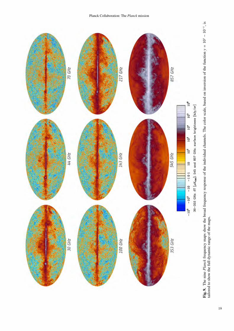
Planck Collaboration: The Planck mission
Fig.
9.T
heni
neP
lanc
kfr
eque
ncy
map
ssh
owth
ebr
oad
freq
uenc
yre
spon
seof
the
indi
vidu
alch
anne
ls.T
heco
lor
scal
e,ba
sed
onin
vers
ion
ofth
efu
nctio
ny
=10
x−
10−x
,is
tailo
red
tosh
owth
efu
lldy
nam
icra
nge
ofth
em
aps.
19
Planck Collaboration: The Planck mission
same spectral energy distribution (SED) within the bandpass asthe calibrator, the true brightness is the ratio of the response tothe target and the response to the calibrator. In practice onlyCMB anisotropies satisfy this condition; other sources of radia-tion have different SEDs. The raw brightness values in the mapscannot then be taken as monochromatic values; rather, they rep-resent the integral of the detected power weighted by the band-pass.
To allow comparison with other measurements and withmodels, the brightness of the CMB-calibrated channels is givenas differential CMB temperature, ∆TCMB = ∆Iν/(dBν/dT )T0 ,where Bν is the Planck function, T0 = 2.7255 K (Fixsen 2009),and ν is a specified reference frequency for each channel10. Theunits are thermodynamic temperature, KCMB.
The 545 and 857 GHz channel maps are instead given inintensity units (MJy sr−1), assuming the reference SED Iν =I0 × (ν0/ν) (used previously by IRAS and COBE-DIRBE). Forall Planck channels, the intensity (or flux density for unresolvedsources) is attached to a choice of both reference frequency andassumed SED.
Each foreground observed by Planck has a different SED(power law, modified black body, SZ distortion, CO lines). Toevaluate intensities for these SEDs, e.g., for component sepa-ration, we provide unit conversions and colour corrections foreach band, where the corrected values are such that the powerintegrated in the spectral bandpass and throughput is equal tothe measured power. These are described for LFI in PlanckCollaboration V (2014), which tabulates conversion from theCMB fluctuation SED to power-laws with various indices, andfor HFI in Planck Collaboration IX (2014), which gives conver-sions between the two standard HFI SEDs (CMB fluctuation andIRAS standard), and also the Compton ysz parameter. In addition,a unit conversion and colour correction software tool (UcCC)covering all Planck bands is provided as part of the data releaseand described in Planck Collaboration IX (2014). Users are cau-tioned to read the detailed descriptions carefully, as in general asequence of steps is required to convert from the units and as-sumed SED of the map calibration to the those appropriate fora given foreground. Our colour conversions are uniformly castas a multiplicative correction, yielding the brightness at the stan-dard band reference frequency for the required SED. It wouldalso have been possible in most cases to quote an “effective fre-quency” at which the numerical value of the map brightness ap-plies to the required SED, but this is less practical in general andcannot be applied at all to line emission. The effective frequen-cies for the LFI detectors in Table 2 correspond to the SED forthe CMB.
6.4. Map characterization
Null tests are a powerful way to evaluate the quality of LFIand HFI maps. Among these are half-ring difference maps(which capture noise properties), and Survey-to-Survey differ-ences (which capture different types of systematic signals).Simulation of known systematics is also a viable way to validatethe effects seen in the real data, especially in Survey-to-Surveydifferences. Comparison of angular cross-power spectra of mapsmade with individual detectors within a frequency band, and ofmaps at different frequencies, is used to give confidence in theresults. Many such tests have been implemented, as described
10 Our definition of ∆TCMB is linearized, and deviates significantlyfrom the true variation in the equivalent blackbody temperature in thebrightest regions of the 217 and 353 GHz maps.
in Planck Collaboration II (2014), Planck Collaboration III(2014), and Planck Collaboration V (2014) for LFI, and PlanckCollaboration VI (2014), Planck Collaboration VII (2014),Planck Collaboration VIII (2014), and Planck Collaboration IX(2014) for HFI. Table 5 summarises the sources contributingto uncertainties at map level. Table 6 gives the actual uncer-tainty levels for each map. For residual systematic levels, seePlanck Collaboration III (2014) (LFI) and Planck CollaborationVI (2014) (HFI).
6.5. Consistency tests
One of the key design features of Planck is that it contains twoseparate instruments, subject to independent calibration and sys-tematic effects. The simple fact that they observe the same CMBanisotropies in nearly adjacent frequency bands, and that theydo so with high signal-to-noise ratio, provides a powerful cross-check on data quality. However, the very high accuracy (∼0.1 %)that is the aim of Planck also implies that every minute differ-ence in how the CMB anisotropies are observed must be takeninto account when comparing data from LFI and HFI. This ap-plies particularly to instrumental issues (beam shapes, noise lev-els) and residual foreground signals. Similar considerations ap-ply when comparing Planck data to data from other experiments,e.g. WMAP.
Figure 10 shows a map-level comparison between 70 and100 GHz, the closest frequencies between the two instruments.The CMB structures at high Galactic latitude disappear in thedifference made in Kcmb units as shown by the uniform back-ground of noise. The deep nulling of the CMB anisotropy signaldirectly achieved by this straightforward differencing demon-strates that the Planck maps are free from serious large- tointermediate-scale imperfections. It also reveals in an immedi-ate and interesting manner the foreground residuals.
Spectral analysis allows a more quantitative assessment. Theresult of a detailed comparison between neighbouring maps at70, 100, and 143 GHz is shown in Figure 11, checking con-sistency between LFI and HFI, and agreement between themain CMB channels overall. In doing this comparison, resid-ual foregrounds cannot be ignored (see Section 8.3, Figures 27and 28) and are corrected for channel-by-channel. Beam effectsalso have to be taken into account for such spectral compar-isons. Since the data release of March 2013, strong evidencehas arisen that a small fraction (∼0.2 %) of the HFI beams’solid angle was not taken into account in the window func-tions (Section 5.4), and a correction for this has been includedin Figure 11. See Planck Collaboration VII (2014) and PlanckCollaboration XXXI (2014) for a complete description.
Figure 11 demonstrates that, once residual foregrounds andknown beam effects are corrected for, spectral consistency be-tween the LFI 70 GHz and HFI 100 GHz maps is achieved at alevel of 0.43 % , and between the HFI 100 and 143 GHz chan-nels at a level of 0.46 % (the values quoted are averages between` = 70 and 390). These consistency levels are within the uncer-tainties assumed for the 2013 scientific analysis.
Additional checks can be made. For example, Fig. 12(Planck Collaboration VI 2014) compares CMB anisotropies inall Planck LFI and HFI channels (44, 70, 100, 143, 217, 353GHz) following component separation at the power spectrumlevel and using 143 GHz as the reference. The three main HFICMB channels agree within 0.3 % of each other. The recalibra-tion coefficients for the bands 70 to 217 GHz are all within 0.4 %;44 and 353 GHz are at the 2 % level.
20
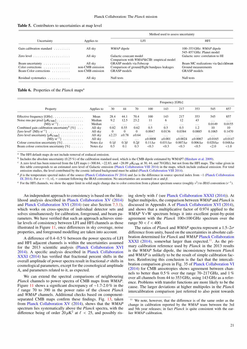
Planck Collaboration: The Planck mission
Table 5. Contributors to uncertainties at map level
Method used to assess uncertainty
Uncertainty Applies to LFI HFI
Gain calibration standard . . . . . . . . All sky WMAP dipole 100–353 GHz: WMAP dipole545–857 GHz: Planet model
Zero level . . . . . . . . . . . . . . . . . . All sky Galactic cosecant model Galactic zero: correlation to HIComparison with WMAP&CIB: empirical model
Beam uncertainty . . . . . . . . . . . . . All sky GRASP models via Febecop Beam MC realizations via QuickbeamColor corrections . . . . . . . . . . . . . non-CMB emission Comparison of ground/flight bandpass leakages Ground measurementsBeam Color corrections . . . . . . . . . non-CMB emission GRASP models GRASP models
Residual systematics . . . . . . . . . . . All sky Null tests Null tests
Table 6. Properties of the Planck mapsa
Frequency [GHz]
Property Applies to 30 44 70 100 143 217 353 545 857
Effective frequency [GHz] . . . . . . . . . . . . . . . Mean 28.4 44.1 70.4 100 143 217 353 545 857Noise rms per pixel [µKCMB] . . . . . . . . . . . . . Median 9.2 12.5 23.2 11 6 12 43 . . . . . .
[MJy sr−1] . . . . . . . . . . . . Median . . . . . . . . . . . . . . . . . . . . . 0.0149 0.0155Combined gain calibration uncertaintyb [%] . . . All sky 0.82 0.55 0.62 0.5 0.5 0.5 1.2 10 10Zero levelc [MJy sr−1] . . . . . . . . . . . . . . . . . All sky 0 0 0 0.0047 0.0136 0.0384 0.0885 0.1065 0.1470Zero level uncertainty [µKCMB] . . . . . . . . . . . All sky ±2.23 ±0.78 ±0.64 . . . . . . . . . . . . . . . . . .
[MJy sr−1] . . . . . . . . . . All sky . . . . . . . . . ±0.0008 ±0.001 ±0.0024 ±0.0067 ±0.0165 ±0.0147Colour correction uncertainty [%] . . . . . . . . . . Notes d,e 0.1β 0.3β 0.2β 0.11∆α 0.031∆α 0.007∆α 0.006∆α 0.020∆α 0.048∆αBeam colour correction uncertainty [%] . . . . . . Notes d,e 0.5 0.1 0.3 <0.3 <0.3 <0.3 <0.5 <2.0 <1.0
a The HFI default maps do not include removal of zodiacal emission.b Includes the absolute uncertainty (0.25 %) of the calibration standard used, which is the CMB dipole estimated by WMAP7 (Hinshaw et al. 2009).c A zero level has been removed from the LFI maps (−300.84, −22.83, and −28.09 µKCMB at 30, 44, and 70 GHz), but not from the HFI maps. The value given in
this table corresponds to an estimated zero level of Galactic emission (Planck Collaboration VIII 2014) in the maps, which include zodiacal emission. For totalemission studies, the level contributed by the cosmic infrared background must be added (Planck Collaboration VIII 2014).
d β is the temperature spectral index of the source (Planck Collaboration IV 2014) and ∆α is the difference in source spectral index from −1 (Planck CollaborationIX 2014). For α = −1, νIν = constant following the IRAS convention. No uncertainties are assumed on α and β.
e For the HFI channels, we show the upper limit in solid angle change due to color correction from a planet spectrum source (roughly ν2) to IRAS convention (ν−1).
An independent approach to consistency is based on the like-lihood analysis described in Planck Collaboration XV (2014)and Planck Collaboration XVI (2014) (see also Section 7.3.1),which works on cross-spectra of individual detector sets andsolves simultaneously for calibration, foreground, and beam pa-rameters. We have verified that such an approach achieves simi-lar levels of consistency between LFI and HFI channels as thoseillustrated in Figure 11, once differences in sky coverage, noiseproperties, and foreground modelling are taken into account.
A difference of 0.4–0.5 % between the power spectra of LFIand HFI adjacent channels is within the uncertainties assumedfor the 2013 scientific analysis (Planck Collaboration XVI2014). A specific analysis described in Planck CollaborationXXXI (2014) has verified that fractional percent shifts in theoverall amplitude of power spectra result in fractional σ shifts incosmological parameters, except for the cosmological amplitudeAs and parameters related to it, as expected.
We can extend the spectral comparisons of neighbouringPlanck channels to power spectra of CMB maps from WMAP.Figure 11 shows a significant discrepancy of ∼1.7-2.0 % in the` range 70 to 390 in the power ratio of the closest Planckand WMAP channels. Additional checks based on component-separated CMB maps confirm these findings. Fig. 13, takenfrom Planck Collaboration XV (2014), shows that the WMAPspectrum lies systematically above the Planck spectra, with thedifference being of order 20 µK2 at ` < 25, and possibly ris-
ing slowly with ` (see Planck Collaboration XXXI (2014)). Athigher multipoles, the comparison between WMAP and Planck isdiscussed in Appendix A of Planck Collaboration XVI (2014),and shows that a multiplicative factor of 0.974 applied to theWMAP V+W spectrum brings it into excellent point-by-pointagreement with the Planck 100×100 GHz spectrum over therange 50 < ` < 400.
The ratios of Planck and WMAP spectra represent a 1.5–2σdifference from unity, based on the uncertainties in absolute cali-bration determined for Planck and WMAP Planck CollaborationXXXI (2014), somewhat larger than expected.11. As the pri-mary calibration reference used by Planck in the 2013 resultsis the WMAP Solar dipole, the inconsistency between Planckand WMAP is unlikely to be the result of simple calibration fac-tors. Reinforcing this conclusion is the fact that the intercali-bration comparison given in Fig. 35 of Planck Collaboration VI(2014) for CMB anisotropies shows agreement between chan-nels to better than 0.5 % over the range 70–217 GHz, and 1 %over all channels from 44 to 353 GHz, using 143 GHz as a refer-ence. Problems with transfer functions are more likely to be thecause. The larger deviations at higher multipoles in the Planckintercalibration comparison just referred to also point towards
11 We note, however, that the difference is of the same order as thechange in calibration reported by the WMAP team between the 3rdand 5th year releases; in fact Planck is quite consistent with the ear-lier WMAP calibration.
21
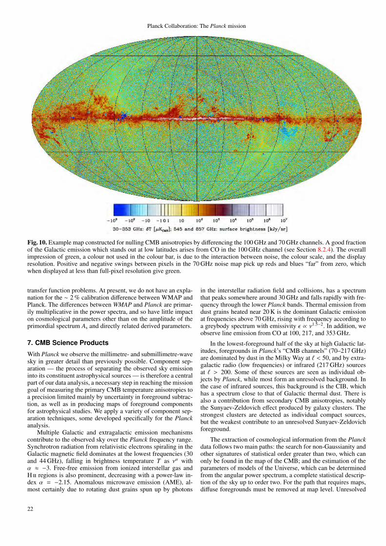
Planck Collaboration: The Planck mission
Fig. 10. Example map constructed for nulling CMB anisotropies by differencing the 100 GHz and 70 GHz channels. A good fractionof the Galactic emission which stands out at low latitudes arises from CO in the 100 GHz channel (see Section 8.2.4). The overallimpression of green, a colour not used in the colour bar, is due to the interaction between noise, the colour scale, and the displayresolution. Positive and negative swings between pixels in the 70 GHz noise map pick up reds and blues “far” from zero, whichwhen displayed at less than full-pixel resolution give green.
transfer function problems. At present, we do not have an expla-nation for the ∼ 2 % calibration difference between WMAP andPlanck. The differences between WMAP and Planck are primar-ily multiplicative in the power spectra, and so have little impacton cosmological parameters other than on the amplitude of theprimordial spectrum As and directly related derived parameters.
7. CMB Science Products
With Planck we observe the millimetre- and submillimetre-wavesky in greater detail than previously possible. Component sep-aration — the process of separating the observed sky emissioninto its constituent astrophysical sources — is therefore a centralpart of our data analysis, a necessary step in reaching the missiongoal of measuring the primary CMB temperature anisotropies toa precision limited mainly by uncertainty in foreground subtrac-tion, as well as in producing maps of foreground componentsfor astrophysical studies. We apply a variety of component sep-aration techniques, some developed specifically for the Planckanalysis.
Multiple Galactic and extragalactic emission mechanismscontribute to the observed sky over the Planck frequency range.Synchrotron radiation from relativistic electrons spiraling in theGalactic magnetic field dominates at the lowest frequencies (30and 44 GHz), falling in brightness temperature T as να withα ≈ −3. Free-free emission from ionized interstellar gas andH ii regions is also prominent, decreasing with a power-law in-dex α = −2.15. Anomalous microwave emission (AME), al-most certainly due to rotating dust grains spun up by photons
in the interstellar radiation field and collisions, has a spectrumthat peaks somewhere around 30 GHz and falls rapidly with fre-quency through the lower Planck bands. Thermal emission fromdust grains heated near 20 K is the dominant Galactic emissionat frequencies above 70 GHz, rising with frequency according toa greybody spectrum with emissivity ε ∝ ν1.5−2. In addition, weobserve line emission from CO at 100, 217, and 353 GHz.
In the lowest-foreground half of the sky at high Galactic lat-itudes, foregrounds in Planck’s “CMB channels” (70–217 GHz)are dominated by dust in the Milky Way at ` < 50, and by extra-galactic radio (low frequencies) or infrared (217 GHz) sourcesat ` > 200. Some of these sources are seen as individual ob-jects by Planck, while most form an unresolved background. Inthe case of infrared sources, this background is the CIB, whichhas a spectrum close to that of Galactic thermal dust. There isalso a contribution from secondary CMB anisotropies, notablythe Sunyaev-Zeldovich effect produced by galaxy clusters. Thestrongest clusters are detected as individual compact sources,but the weakest contribute to an unresolved Sunyaev-Zeldovichforeground.
The extraction of cosmological information from the Planckdata follows two main paths: the search for non-Gaussianity andother signatures of statistical order greater than two, which canonly be found in the map of the CMB; and the estimation of theparameters of models of the Universe, which can be determinedfrom the angular power spectrum, a complete statistical descrip-tion of the sky up to order two. For the path that requires maps,diffuse foregrounds must be removed at map level. Unresolved
22
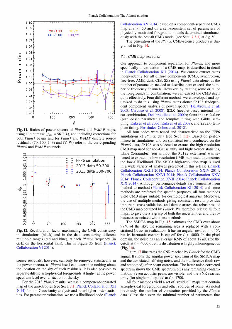
Planck Collaboration: The Planck mission
Fig. 11. Ratios of power spectra of Planck and WMAP maps,using a joint mask ( fsky = 56.7 %), and including corrections forboth Planck beams and for Planck and WMAP discrete sourceresiduals. (70, 100, 143) and (V, W) refer to the correspondingPlanck and WMAP channels.
Fig. 12. Recalibration factor maximizing the CMB consistencyin simulations (black) and in the data considering differentmultipole ranges (red and blue), at each Planck frequency (inGHz on the horizontal axis). This is Figure 35 from (PlanckCollaboration VI 2014).
source residuals, however, can only be removed statistically inthe power spectra, as Planck itself can determine nothing aboutthe location on the sky of such residuals. It is also possible toseparate diffuse astrophysical foregrounds at high-` at the powerspectrum level over a fraction of the sky.
For the 2013 Planck results, we use a component-separatedmap of the anisotropies (see Sect. 7.1, Planck Collaboration XII2014) for non-Gaussianity analysis and other higher-order statis-tics. For parameter estimation, we use a likelihood code (Planck
Collaboration XV 2014) based on a component-separated CMBmap at ` < 50 and on a self-consistent set of parameters ofphysically-motivated foreground models determined simultane-ously with the best-fit CMB model (see Sect. 7.3.1) at ` ≥ 50.
The generation of the Planck CMB-science products is dia-gramed in Fig. 14.
7.1. CMB map extraction
Our approach to component separation for Planck, and morespecifically to extraction of a CMB map, is described in detailin Planck Collaboration XII (2014). We cannot extract mapsindependently for all diffuse components (CMB, synchrotron,free-free, AME, dust, CIB, SZ) using Planck data alone, as thenumber of parameters needed to describe them exceeds the num-ber of frequency channels. However, by treating some or all ofthe foregrounds in combination, we can extract the CMB itselfquite effectively. Four different methods were developed and op-timized to do this using Planck maps alone: SMICA (indepen-dent component analysis of power spectra, Delabrouille et al.2003; Cardoso et al. 2008); NILC (needlet-based internal lin-ear combination, Delabrouille et al. 2009); Commander-Ruler(pixel-based parameter and template fitting with Gibbs sam-pling, Eriksen et al. 2006; Eriksen et al. 2008); and SEVEM (tem-plate fitting, Fernandez-Cobos et al. 2012).
All four codes were tested and characterized on the FFP6simulations of Planck data (see Sect. 5.2). Based on perfor-mance in simulations and on statistical tests conducted on thePlanck data, SMICA was selected to extract the high-resolutionCMB map used for non-Gaussianity and higher-order statistics,while Commander (run without the Ruler extension) was se-lected to extract the low-resolution CMB map used to constructthe low-` likelihood. The SMICA high-resolution map is usedin a wide variety of analyses presented in this release (PlanckCollaboration XXIII 2014; Planck Collaboration XXIV 2014;Planck Collaboration XXVI 2014; Planck Collaboration XXV2014; Planck Collaboration XVII 2014; Planck CollaborationXIX 2014). Although performance details vary somewhat frommethod to method (Planck Collaboration XII 2014) and somemethods are preferred for specific purposes, all four methodsyield CMB maps suitable for cosmological analysis. Moreover,the use of multiple methods giving consistent results providesimportant cross-validation, and demonstrates the robustness ofthe CMB map obtained by Planck. We therefore release all fourmaps, to give users a grasp of both the uncertainties and the ro-bustness associated with these methods.
The SMICA map in Fig. 15 estimates the CMB over about97 % of the sky; the remaining area is replaced with a con-strained Gaussian realization. It has an angular resolution of 5′,but its harmonic content is cut off for ` > 4000. In the pixeldomain, the noise has an average RMS of about 17 µK (for thecutoff at ` = 4000), but its distribution is highly inhomogeneous(Fig. 16).
Figure 17 illustrates the SNR reached by Planck for the CMBsignal. It shows the angular power spectrum of the SMICA mapand the associated half-ring noise, and their difference (both rawand smoothed) after beam correction. The latter noise-correctedspectrum shows the CMB spectrum plus any remaining contam-ination. Seven acoustic peaks are visible, and the SNR reachesunity (for single multipoles) at ` ∼ 1700.
All four methods yield a set of “residual” maps that containastrophysical foregrounds and other sources of noise. As notedpreviously, the number of constraints provided by the Planckdata is less than even the minimal number of parameters that
23
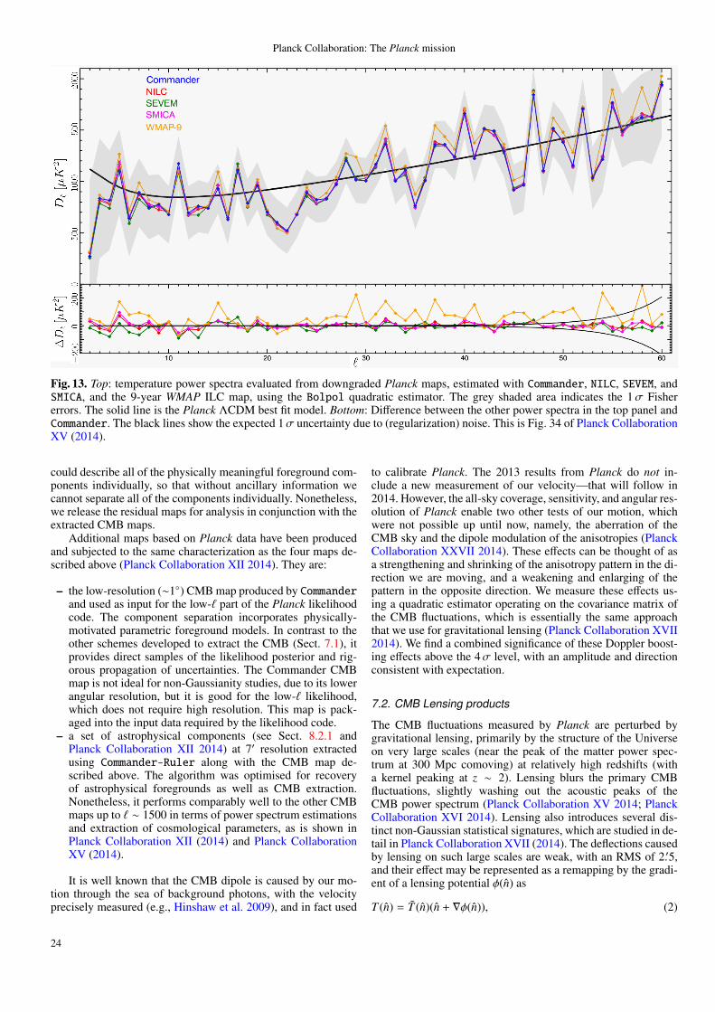
Planck Collaboration: The Planck mission
Fig. 13. Top: temperature power spectra evaluated from downgraded Planck maps, estimated with Commander, NILC, SEVEM, andSMICA, and the 9-year WMAP ILC map, using the Bolpol quadratic estimator. The grey shaded area indicates the 1σ Fishererrors. The solid line is the Planck ΛCDM best fit model. Bottom: Difference between the other power spectra in the top panel andCommander. The black lines show the expected 1σ uncertainty due to (regularization) noise. This is Fig. 34 of Planck CollaborationXV (2014).
could describe all of the physically meaningful foreground com-ponents individually, so that without ancillary information wecannot separate all of the components individually. Nonetheless,we release the residual maps for analysis in conjunction with theextracted CMB maps.
Additional maps based on Planck data have been producedand subjected to the same characterization as the four maps de-scribed above (Planck Collaboration XII 2014). They are:
– the low-resolution (∼1) CMB map produced by Commanderand used as input for the low-` part of the Planck likelihoodcode. The component separation incorporates physically-motivated parametric foreground models. In contrast to theother schemes developed to extract the CMB (Sect. 7.1), itprovides direct samples of the likelihood posterior and rig-orous propagation of uncertainties. The Commander CMBmap is not ideal for non-Gaussianity studies, due to its lowerangular resolution, but it is good for the low-` likelihood,which does not require high resolution. This map is pack-aged into the input data required by the likelihood code.
– a set of astrophysical components (see Sect. 8.2.1 andPlanck Collaboration XII 2014) at 7′ resolution extractedusing Commander-Ruler along with the CMB map de-scribed above. The algorithm was optimised for recoveryof astrophysical foregrounds as well as CMB extraction.Nonetheless, it performs comparably well to the other CMBmaps up to ` ∼ 1500 in terms of power spectrum estimationsand extraction of cosmological parameters, as is shown inPlanck Collaboration XII (2014) and Planck CollaborationXV (2014).
It is well known that the CMB dipole is caused by our mo-tion through the sea of background photons, with the velocityprecisely measured (e.g., Hinshaw et al. 2009), and in fact used
to calibrate Planck. The 2013 results from Planck do not in-clude a new measurement of our velocity—that will follow in2014. However, the all-sky coverage, sensitivity, and angular res-olution of Planck enable two other tests of our motion, whichwere not possible up until now, namely, the aberration of theCMB sky and the dipole modulation of the anisotropies (PlanckCollaboration XXVII 2014). These effects can be thought of asa strengthening and shrinking of the anisotropy pattern in the di-rection we are moving, and a weakening and enlarging of thepattern in the opposite direction. We measure these effects us-ing a quadratic estimator operating on the covariance matrix ofthe CMB fluctuations, which is essentially the same approachthat we use for gravitational lensing (Planck Collaboration XVII2014). We find a combined significance of these Doppler boost-ing effects above the 4σ level, with an amplitude and directionconsistent with expectation.
7.2. CMB Lensing products
The CMB fluctuations measured by Planck are perturbed bygravitational lensing, primarily by the structure of the Universeon very large scales (near the peak of the matter power spec-trum at 300 Mpc comoving) at relatively high redshifts (witha kernel peaking at z ∼ 2). Lensing blurs the primary CMBfluctuations, slightly washing out the acoustic peaks of theCMB power spectrum (Planck Collaboration XV 2014; PlanckCollaboration XVI 2014). Lensing also introduces several dis-tinct non-Gaussian statistical signatures, which are studied in de-tail in Planck Collaboration XVII (2014). The deflections causedby lensing on such large scales are weak, with an RMS of 2.′5,and their effect may be represented as a remapping by the gradi-ent of a lensing potential φ(n) as
T (n) = T (n)(n + ∇φ(n)), (2)
24
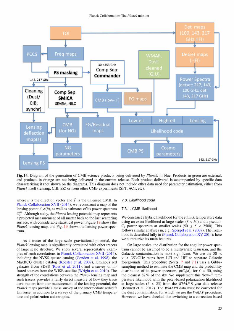
Planck Collaboration: The Planck mission
!"#$%&'()% *#+)#+%&'()%,-!./%
01&(%2#(3%!"#$%&
245467%8.90%
06:%%,;1"%8</%
!<=>#)?@A'B%&'()%
C1D#"%2(#E+"'%,@#+)#+3%FGH7%GIJ7%GKK%<-LM%@#+3%GIJ7%FGH%<-L/%
N6OC7%*A)+PEB#'Q#@%,R7S/%%
06:%C2% 01)&1%('"'&#+#")%
06:%,B1DPl /%
*#+%%&'()%,GKK7%GIJ7%FGH%
<-L%-!./%TU.%
01&(%2#(3%$'(()*+,-&&.!&()/01*2&
C002%
9?V#B?W11@%E1@#%
91DP#BB% -?XWP#BB% 9#Q)?QX%
9#Q)?QX%C2%
9#Q)?QX%@#Y#EZ1Q%&'(,)/%
GIJ7%FGH%<-L%
0B#'Q?QX%,*A)+=0.:7%
)[QEW"/%
GIJ7%FGH%<-L%
8<%('"'&#+#")%
JKP\J]J%<-L%
!<%&'()%
Fig. 14. Diagram of the generation of CMB-science products being delivered by Planck, in blue. Products in green are external,and products in orange are not being delivered in the current release. Each product delivered is accompanied by specific datacharacterizing it (not shown on the diagram). This diagram does not include other data used for parameter estimation, either fromPlanck itself (lensing, CIB, SZ) or from other CMB experiments (SPT, ACT, etc).
where n is the direction vector and T is the unlensed CMB. InPlanck Collaboration XVII (2014), we reconstruct a map of thelensing potential φ(n), as well as estimates of its power spectrumCφφ
L . Although noisy, the Planck lensing potential map representsa projected measurement of all matter back to the last scatteringsurface, with considerable statistical power. Figure 18 shows thePlanck lensing map, and Fig. 19 shows the lensing power spec-trum.
As a tracer of the large scale gravitational potential, thePlanck lensing map is significantly correlated with other tracersof large scale structure. We show several representative exam-ples of such correlations in Planck Collaboration XVII (2014),including the NVSS quasar catalog (Condon et al. 1998), theMaxBCG cluster catalog (Koester et al. 2007), luminous redgalaxies from SDSS (Ross et al. 2011), and a survey of in-frared sources from the WISE satellite (Wright et al. 2010). Thestrength of the correlations between the Planck lensing map andsuch tracers provides a fairly direct measure of how they tracedark matter; from our measurement of the lensing potential, thePlanck maps provide a mass survey of the intermediate redshiftUniverse, in addition to a survey of the primary CMB tempera-ture and polarization anisotropies.
7.3. Likelihood code
7.3.1. CMB likelihood
We construct a hybrid likelihood for the Planck temperature datausing an exact likelihood at large scales (` < 50) and a pseudo-C` power spectrum at smaller scales (50 ≤ ` < 2500). Thisfollows similar analyses in, e.g., Spergel et al. (2007). The likeli-hood is described fully in (Planck Collaboration XV 2014); herewe summarize its main features.
On large scales, the distribution for the angular power spec-trum cannot be assumed to be a multivariate Gaussian, and theGalactic contamination is most significant. We use the 30 <ν < 353 GHz maps from LFI and HFI to separate Galacticforegrounds. This procedure (Sects. 7 and 7.1) uses a Gibbs-sampling method to estimate the CMB map and the probabilitydistribution of its power spectrum, p(C` |d), for ` < 50, usingthe cleanest 87 % of the sky. We supplement this ‘low-`’ tem-perature likelihood with the pixel-based polarization likelihoodat large scales (` < 23) from the WMAP 9-year data release(Bennett et al. 2012). The WMAP9 data must be corrected forthe dust contamination, for which we use the WMAP procedure.However, we have checked that switching to a correction based
25
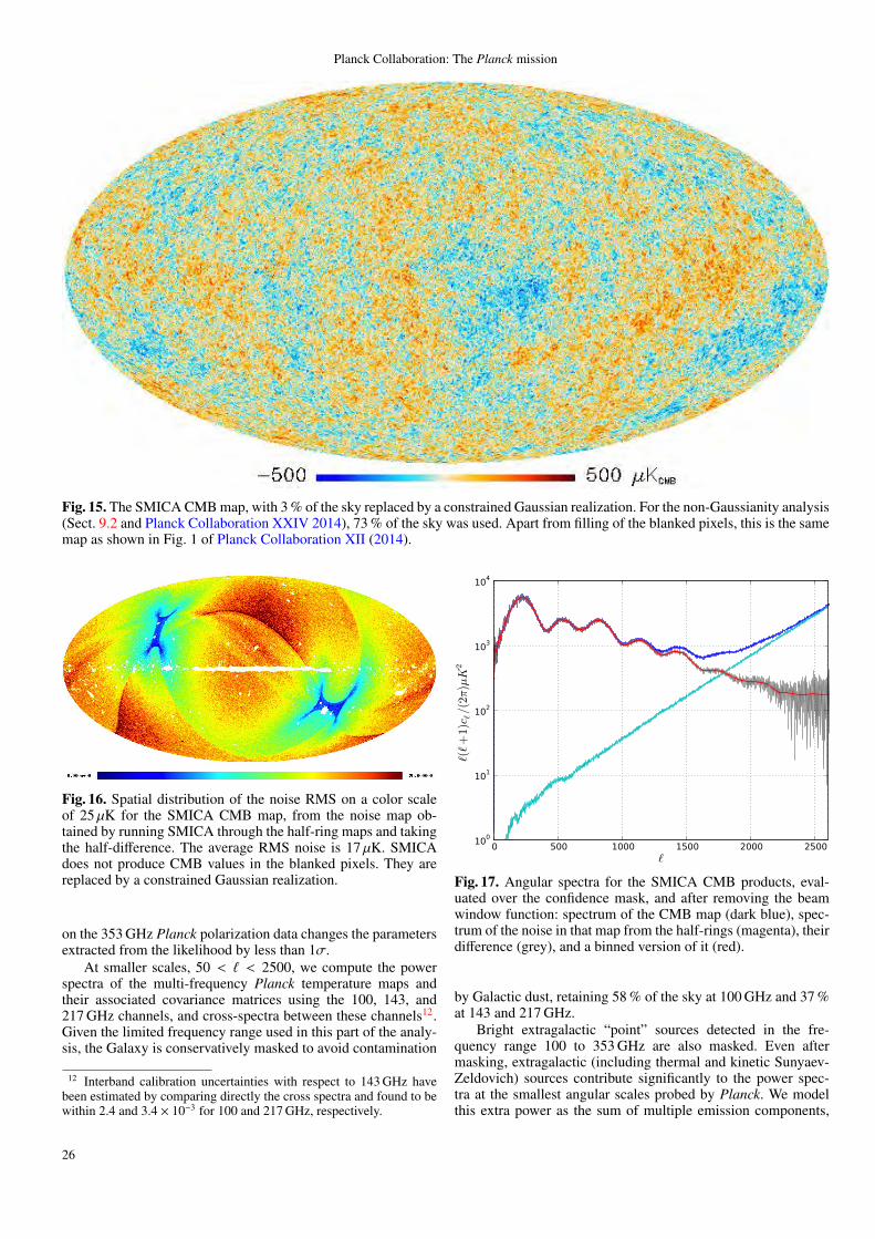
Planck Collaboration: The Planck mission
Fig. 15. The SMICA CMB map, with 3 % of the sky replaced by a constrained Gaussian realization. For the non-Gaussianity analysis(Sect. 9.2 and Planck Collaboration XXIV 2014), 73 % of the sky was used. Apart from filling of the blanked pixels, this is the samemap as shown in Fig. 1 of Planck Collaboration XII (2014).
Fig. 16. Spatial distribution of the noise RMS on a color scaleof 25 µK for the SMICA CMB map, from the noise map ob-tained by running SMICA through the half-ring maps and takingthe half-difference. The average RMS noise is 17 µK. SMICAdoes not produce CMB values in the blanked pixels. They arereplaced by a constrained Gaussian realization.
on the 353 GHz Planck polarization data changes the parametersextracted from the likelihood by less than 1σ.
At smaller scales, 50 < ` < 2500, we compute the powerspectra of the multi-frequency Planck temperature maps andtheir associated covariance matrices using the 100, 143, and217 GHz channels, and cross-spectra between these channels12.Given the limited frequency range used in this part of the analy-sis, the Galaxy is conservatively masked to avoid contamination
12 Interband calibration uncertainties with respect to 143 GHz havebeen estimated by comparing directly the cross spectra and found to bewithin 2.4 and 3.4 × 10⁻³ for 100 and 217 GHz, respectively.
Fig. 17. Angular spectra for the SMICA CMB products, eval-uated over the confidence mask, and after removing the beamwindow function: spectrum of the CMB map (dark blue), spec-trum of the noise in that map from the half-rings (magenta), theirdifference (grey), and a binned version of it (red).
by Galactic dust, retaining 58 % of the sky at 100 GHz and 37 %at 143 and 217 GHz.
Bright extragalactic “point” sources detected in the fre-quency range 100 to 353 GHz are also masked. Even aftermasking, extragalactic (including thermal and kinetic Sunyaev-Zeldovich) sources contribute significantly to the power spec-tra at the smallest angular scales probed by Planck. We modelthis extra power as the sum of multiple emission components,
26
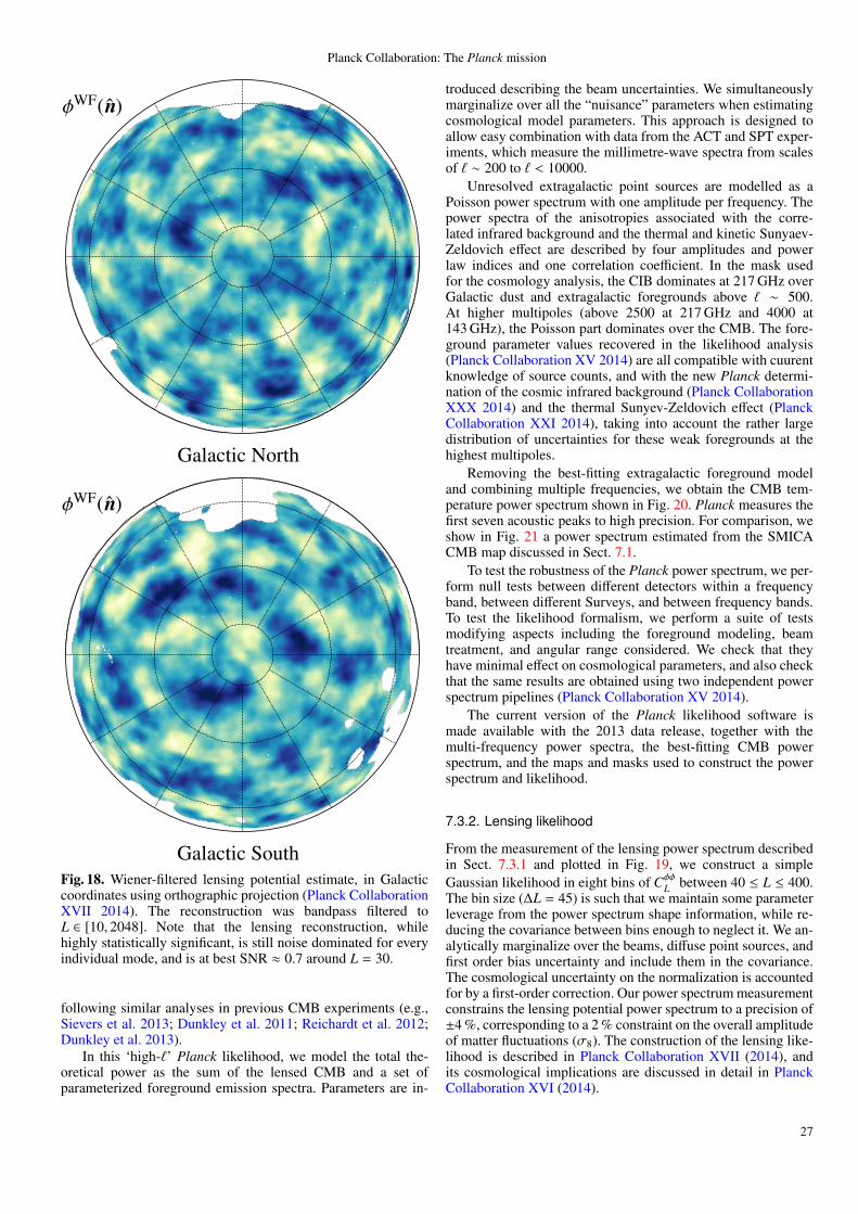
Planck Collaboration: The Planck missionPlanck Collaboration: Gravitational lensing by large-scale structures with Planck
φWF(n)
Galactic North
φWF(n)
Galactic South
Fig. 8. Wiener-filtered lensing potential estimateφWF
LM ≡ CφφL (φLM − φMF
LM) for our MV reconstruction, in Galacticcoordinates using orthographic projection. The reconstructionis bandpass filtered to L ∈ [10, 2048]. The Planck lens recon-struction has S/N ≤ 1 for individual modes on all scales, sothis map is noise dominated. Comparison between simulationsof reconstructed and input φ in Fig. 4 show the expected levelof visible correlation between our reconstruction and the truelensing potential.
Galactic South - 143 GHz Galactic South - 217 GHz
Fig. 9. Wiener-filtered lensing potential estimates, as in Fig. 8,for the individual 143 and 217 GHz maps. Note that the “noise”due to CMB fluctuations is correlated between these two esti-mates.
on the amplitude of the lensing potential power spectrum, whilethe constraint from current ACT and SPT measurements are32% and 16% respectively. These measurements are neverthe-less quite complementary. As a function of angular scale, thefull-sky Planck power spectrum estimate has the smallest un-certainty per multipole of all three experiments at L < 500, atwhich point the additional small-scale modes up to max = 3000used in the SPT lensing analysis lead to smaller error bars. Thegood agreement in these estimates of Cφφ
L is reassuring; in addi-tion to the fact that the experiments and analyses are completelyindependent, these measurements are sourced from fairly inde-pendent angular scales in the temperature map, with <∼ 1600 inthe case of Planck, < 2300 in the case of ACT, and < 3000in the case of SPT. Cross-correlation of the Planck lensing mapwith these independent measures of the lensing potential willprovide an additional cross-check on their consistency, howeverat the power spectrum level they are already in good agreement.
L
Fig. 11. Replotting of Fig. 10, removing 100 GHz for easiercomparison of 143 and 217 GHz. Also plotted are the SPT band-powers from ?, and the ACT bandpowers from ?. All three ex-periments are very consistent. The lower panel shows the differ-ence between the measured bandpowers and the fiducial best-fitΛCDM model.
6.1. Parameters
Weak gravitational lensing of the CMB provides sensitivityto cosmological parameters affecting the late-time growth ofstructure which are otherwise degenerate in the primary CMBanisotropies imprinted around recombination. Examples includethe dark energy density in models with spatial curvature and the
14
Planck Collaboration: Gravitational lensing by large-scale structures with Planck
φWF(n)
Galactic North
φWF(n)
Galactic South
Fig. 8. Wiener-filtered lensing potential estimateφWF
LM ≡ CφφL (φLM − φMF
LM) for our MV reconstruction, in Galacticcoordinates using orthographic projection. The reconstructionis bandpass filtered to L ∈ [10, 2048]. The Planck lens recon-struction has S/N ≤ 1 for individual modes on all scales, sothis map is noise dominated. Comparison between simulationsof reconstructed and input φ in Fig. 4 show the expected levelof visible correlation between our reconstruction and the truelensing potential.
Galactic South - 143 GHz Galactic South - 217 GHz
Fig. 9. Wiener-filtered lensing potential estimates, as in Fig. 8,for the individual 143 and 217 GHz maps. Note that the “noise”due to CMB fluctuations is correlated between these two esti-mates.
on the amplitude of the lensing potential power spectrum, whilethe constraint from current ACT and SPT measurements are32% and 16% respectively. These measurements are neverthe-less quite complementary. As a function of angular scale, thefull-sky Planck power spectrum estimate has the smallest un-certainty per multipole of all three experiments at L < 500, atwhich point the additional small-scale modes up to max = 3000used in the SPT lensing analysis lead to smaller error bars. Thegood agreement in these estimates of Cφφ
L is reassuring; in addi-tion to the fact that the experiments and analyses are completelyindependent, these measurements are sourced from fairly inde-pendent angular scales in the temperature map, with <∼ 1600 inthe case of Planck, < 2300 in the case of ACT, and < 3000in the case of SPT. Cross-correlation of the Planck lensing mapwith these independent measures of the lensing potential willprovide an additional cross-check on their consistency, howeverat the power spectrum level they are already in good agreement.
L
Fig. 11. Replotting of Fig. 10, removing 100 GHz for easiercomparison of 143 and 217 GHz. Also plotted are the SPT band-powers from ?, and the ACT bandpowers from ?. All three ex-periments are very consistent. The lower panel shows the differ-ence between the measured bandpowers and the fiducial best-fitΛCDM model.
6.1. Parameters
Weak gravitational lensing of the CMB provides sensitivityto cosmological parameters affecting the late-time growth ofstructure which are otherwise degenerate in the primary CMBanisotropies imprinted around recombination. Examples includethe dark energy density in models with spatial curvature and the
14
Fig. 18. Wiener-filtered lensing potential estimate, in Galacticcoordinates using orthographic projection (Planck CollaborationXVII 2014). The reconstruction was bandpass filtered toL ∈ [10, 2048]. Note that the lensing reconstruction, whilehighly statistically significant, is still noise dominated for everyindividual mode, and is at best SNR ≈ 0.7 around L = 30.
following similar analyses in previous CMB experiments (e.g.,Sievers et al. 2013; Dunkley et al. 2011; Reichardt et al. 2012;Dunkley et al. 2013).
In this ‘high-`’ Planck likelihood, we model the total the-oretical power as the sum of the lensed CMB and a set ofparameterized foreground emission spectra. Parameters are in-
troduced describing the beam uncertainties. We simultaneouslymarginalize over all the “nuisance” parameters when estimatingcosmological model parameters. This approach is designed toallow easy combination with data from the ACT and SPT exper-iments, which measure the millimetre-wave spectra from scalesof ` ∼ 200 to ` < 10000.
Unresolved extragalactic point sources are modelled as aPoisson power spectrum with one amplitude per frequency. Thepower spectra of the anisotropies associated with the corre-lated infrared background and the thermal and kinetic Sunyaev-Zeldovich effect are described by four amplitudes and powerlaw indices and one correlation coefficient. In the mask usedfor the cosmology analysis, the CIB dominates at 217 GHz overGalactic dust and extragalactic foregrounds above ` ∼ 500.At higher multipoles (above 2500 at 217 GHz and 4000 at143 GHz), the Poisson part dominates over the CMB. The fore-ground parameter values recovered in the likelihood analysis(Planck Collaboration XV 2014) are all compatible with cuurentknowledge of source counts, and with the new Planck determi-nation of the cosmic infrared background (Planck CollaborationXXX 2014) and the thermal Sunyev-Zeldovich effect (PlanckCollaboration XXI 2014), taking into account the rather largedistribution of uncertainties for these weak foregrounds at thehighest multipoles.
Removing the best-fitting extragalactic foreground modeland combining multiple frequencies, we obtain the CMB tem-perature power spectrum shown in Fig. 20. Planck measures thefirst seven acoustic peaks to high precision. For comparison, weshow in Fig. 21 a power spectrum estimated from the SMICACMB map discussed in Sect. 7.1.
To test the robustness of the Planck power spectrum, we per-form null tests between different detectors within a frequencyband, between different Surveys, and between frequency bands.To test the likelihood formalism, we perform a suite of testsmodifying aspects including the foreground modeling, beamtreatment, and angular range considered. We check that theyhave minimal effect on cosmological parameters, and also checkthat the same results are obtained using two independent powerspectrum pipelines (Planck Collaboration XV 2014).
The current version of the Planck likelihood software ismade available with the 2013 data release, together with themulti-frequency power spectra, the best-fitting CMB powerspectrum, and the maps and masks used to construct the powerspectrum and likelihood.
7.3.2. Lensing likelihood
From the measurement of the lensing power spectrum describedin Sect. 7.3.1 and plotted in Fig. 19, we construct a simpleGaussian likelihood in eight bins of Cφφ
L between 40 ≤ L ≤ 400.The bin size (∆L = 45) is such that we maintain some parameterleverage from the power spectrum shape information, while re-ducing the covariance between bins enough to neglect it. We an-alytically marginalize over the beams, diffuse point sources, andfirst order bias uncertainty and include them in the covariance.The cosmological uncertainty on the normalization is accountedfor by a first-order correction. Our power spectrum measurementconstrains the lensing potential power spectrum to a precision of±4 %, corresponding to a 2 % constraint on the overall amplitudeof matter fluctuations (σ8). The construction of the lensing like-lihood is described in Planck Collaboration XVII (2014), andits cosmological implications are discussed in detail in PlanckCollaboration XVI (2014).
27
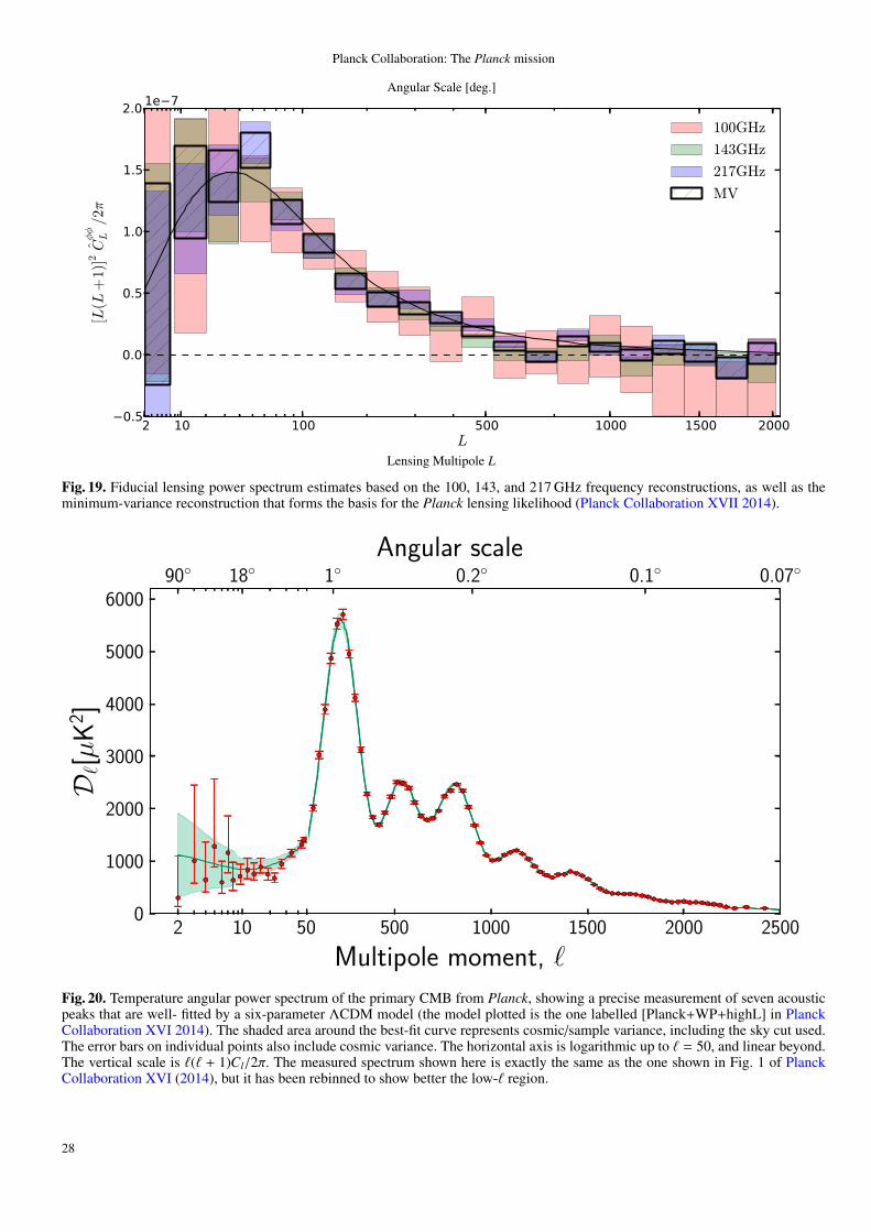
Planck Collaboration: The Planck mission
2 10 100 500 1000 1500 2000L
0.5
0.0
0.5
1.0
1.5
2.0[L
(L+
1)]2Cφφ
L/2π
1e 7
100GHz
143GHz
217GHz
MV
Lensing Multipole L
Angular Scale [deg.]
Fig. 19. Fiducial lensing power spectrum estimates based on the 100, 143, and 217 GHz frequency reconstructions, as well as theminimum-variance reconstruction that forms the basis for the Planck lensing likelihood (Planck Collaboration XVII 2014).
2 10 500
1000
2000
3000
4000
5000
6000
D `[µ
K2 ]
90 18
500 1000 1500 2000 2500
Multipole moment, `
1 0.2 0.1 0.07Angular scale
Fig. 20. Temperature angular power spectrum of the primary CMB from Planck, showing a precise measurement of seven acousticpeaks that are well- fitted by a six-parameter ΛCDM model (the model plotted is the one labelled [Planck+WP+highL] in PlanckCollaboration XVI 2014). The shaded area around the best-fit curve represents cosmic/sample variance, including the sky cut used.The error bars on individual points also include cosmic variance. The horizontal axis is logarithmic up to ` = 50, and linear beyond.The vertical scale is `(` + 1)Cl/2π. The measured spectrum shown here is exactly the same as the one shown in Fig. 1 of PlanckCollaboration XVI (2014), but it has been rebinned to show better the low-` region.
28
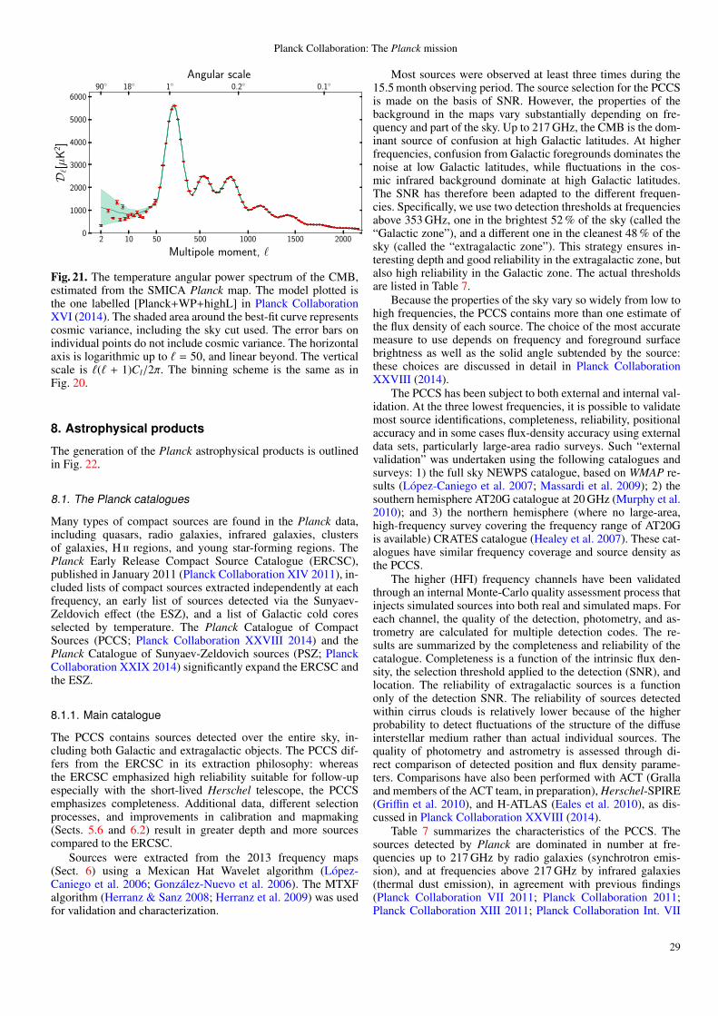
Planck Collaboration: The Planck mission
2 10 500
1000
2000
3000
4000
5000
6000
D `[µ
K2 ]
90 18
500 1000 1500 2000
Multipole moment, `
1 0.2 0.1Angular scale
Fig. 21. The temperature angular power spectrum of the CMB,estimated from the SMICA Planck map. The model plotted isthe one labelled [Planck+WP+highL] in Planck CollaborationXVI (2014). The shaded area around the best-fit curve representscosmic variance, including the sky cut used. The error bars onindividual points do not include cosmic variance. The horizontalaxis is logarithmic up to ` = 50, and linear beyond. The verticalscale is `(` + 1)Cl/2π. The binning scheme is the same as inFig. 20.
8. Astrophysical products
The generation of the Planck astrophysical products is outlinedin Fig. 22.
8.1. The Planck catalogues
Many types of compact sources are found in the Planck data,including quasars, radio galaxies, infrared galaxies, clustersof galaxies, H ii regions, and young star-forming regions. ThePlanck Early Release Compact Source Catalogue (ERCSC),published in January 2011 (Planck Collaboration XIV 2011), in-cluded lists of compact sources extracted independently at eachfrequency, an early list of sources detected via the Sunyaev-Zeldovich effect (the ESZ), and a list of Galactic cold coresselected by temperature. The Planck Catalogue of CompactSources (PCCS; Planck Collaboration XXVIII 2014) and thePlanck Catalogue of Sunyaev-Zeldovich sources (PSZ; PlanckCollaboration XXIX 2014) significantly expand the ERCSC andthe ESZ.
8.1.1. Main catalogue
The PCCS contains sources detected over the entire sky, in-cluding both Galactic and extragalactic objects. The PCCS dif-fers from the ERCSC in its extraction philosophy: whereasthe ERCSC emphasized high reliability suitable for follow-upespecially with the short-lived Herschel telescope, the PCCSemphasizes completeness. Additional data, different selectionprocesses, and improvements in calibration and mapmaking(Sects. 5.6 and 6.2) result in greater depth and more sourcescompared to the ERCSC.
Sources were extracted from the 2013 frequency maps(Sect. 6) using a Mexican Hat Wavelet algorithm (Lopez-Caniego et al. 2006; Gonzalez-Nuevo et al. 2006). The MTXFalgorithm (Herranz & Sanz 2008; Herranz et al. 2009) was usedfor validation and characterization.
Most sources were observed at least three times during the15.5 month observing period. The source selection for the PCCSis made on the basis of SNR. However, the properties of thebackground in the maps vary substantially depending on fre-quency and part of the sky. Up to 217 GHz, the CMB is the dom-inant source of confusion at high Galactic latitudes. At higherfrequencies, confusion from Galactic foregrounds dominates thenoise at low Galactic latitudes, while fluctuations in the cos-mic infrared background dominate at high Galactic latitudes.The SNR has therefore been adapted to the different frequen-cies. Specifically, we use two detection thresholds at frequenciesabove 353 GHz, one in the brightest 52 % of the sky (called the“Galactic zone”), and a different one in the cleanest 48 % of thesky (called the “extragalactic zone”). This strategy ensures in-teresting depth and good reliability in the extragalactic zone, butalso high reliability in the Galactic zone. The actual thresholdsare listed in Table 7.
Because the properties of the sky vary so widely from low tohigh frequencies, the PCCS contains more than one estimate ofthe flux density of each source. The choice of the most accuratemeasure to use depends on frequency and foreground surfacebrightness as well as the solid angle subtended by the source:these choices are discussed in detail in Planck CollaborationXXVIII (2014).
The PCCS has been subject to both external and internal val-idation. At the three lowest frequencies, it is possible to validatemost source identifications, completeness, reliability, positionalaccuracy and in some cases flux-density accuracy using externaldata sets, particularly large-area radio surveys. Such “externalvalidation” was undertaken using the following catalogues andsurveys: 1) the full sky NEWPS catalogue, based on WMAP re-sults (Lopez-Caniego et al. 2007; Massardi et al. 2009); 2) thesouthern hemisphere AT20G catalogue at 20 GHz (Murphy et al.2010); and 3) the northern hemisphere (where no large-area,high-frequency survey covering the frequency range of AT20Gis available) CRATES catalogue (Healey et al. 2007). These cat-alogues have similar frequency coverage and source density asthe PCCS.
The higher (HFI) frequency channels have been validatedthrough an internal Monte-Carlo quality assessment process thatinjects simulated sources into both real and simulated maps. Foreach channel, the quality of the detection, photometry, and as-trometry are calculated for multiple detection codes. The re-sults are summarized by the completeness and reliability of thecatalogue. Completeness is a function of the intrinsic flux den-sity, the selection threshold applied to the detection (SNR), andlocation. The reliability of extragalactic sources is a functiononly of the detection SNR. The reliability of sources detectedwithin cirrus clouds is relatively lower because of the higherprobability to detect fluctuations of the structure of the diffuseinterstellar medium rather than actual individual sources. Thequality of photometry and astrometry is assessed through di-rect comparison of detected position and flux density parame-ters. Comparisons have also been performed with ACT (Grallaand members of the ACT team, in preparation), Herschel-SPIRE(Griffin et al. 2010), and H-ATLAS (Eales et al. 2010), as dis-cussed in Planck Collaboration XXVIII (2014).
Table 7 summarizes the characteristics of the PCCS. Thesources detected by Planck are dominated in number at fre-quencies up to 217 GHz by radio galaxies (synchrotron emis-sion), and at frequencies above 217 GHz by infrared galaxies(thermal dust emission), in agreement with previous findings(Planck Collaboration VII 2011; Planck Collaboration 2011;Planck Collaboration XIII 2011; Planck Collaboration Int. VII
29
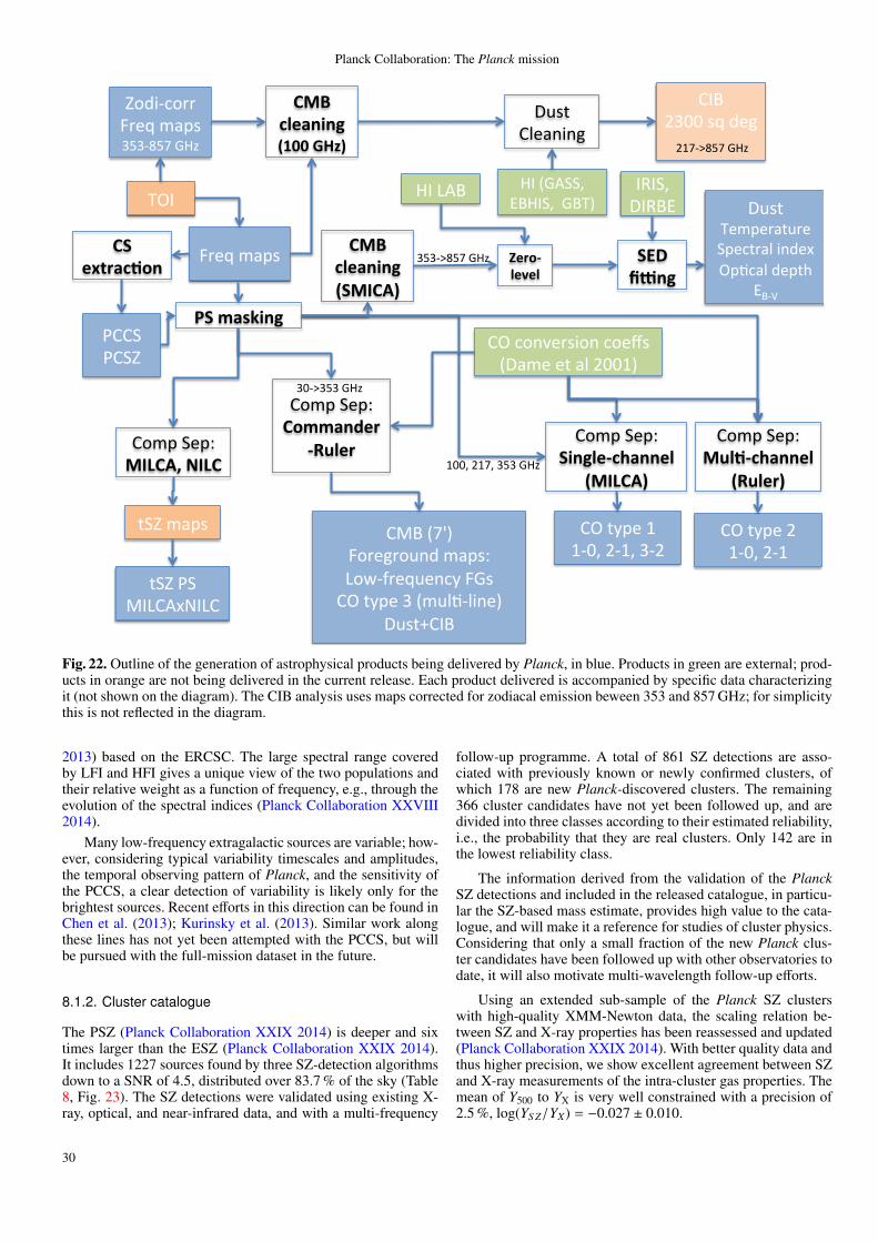
Planck Collaboration: The Planck mission
!"#$%&'()%
*+&(%,#(-%!"#$%&'()*##&%+
,-./012+
*./%0123%!+"#4"+567%&'()-%8+9:;"#$5#6<=%!>)%*?%@=(#%A%0&5BC:BD6#3%
E5)@F*G/%
*?%@=(#%H%H:IJ%K:HJ%A:K%
L?G%
*+&(%,#(-%0344*#5&6
'78%&6+
9!+4*:;"#$+*?%<+6M#")D+6%<+#N)%0E'&#%#@%'B%KIIH3%
E5)@%*B#'6D64+
*G/%%KAII%)$%7#4%
OG%0>P,,J%Q/OG,J%%>/L3%
!<=+>?#$+
GRG,J%EGR/Q% E5)@%
L#&(#"'@5"#%,(#<@"'B%D67#S%?(C<'B%7#(@T%
Q/:U%
*+&(%,#(-%-8%@'()*##&%+
,78%&62+
*?%@=(#%K%H:IJ%K:H%
0-A+(%&*#"#$+,!-.012+
0!+&BC6*(@3#+
V**,%V*,W%
AXA:YZX1%>O[%
OG%8P/%
D&63'+%&E&%+
KH1:YZX1%>O[%
@,W%V,%.G8*PS\G8*%
AI:YAXA%>O[%
HIIJ%KH1J%AXA%>O[%
*+&(%,#(-%-./01F+G./0+
@,W%&'()%
W+7D:<+""%!"#$%&'()%AXA:ZX1%>O[%
0-A+(%&*#"#$+,HII+JKL2+
Fig. 22. Outline of the generation of astrophysical products being delivered by Planck, in blue. Products in green are external; prod-ucts in orange are not being delivered in the current release. Each product delivered is accompanied by specific data characterizingit (not shown on the diagram). The CIB analysis uses maps corrected for zodiacal emission beween 353 and 857 GHz; for simplicitythis is not reflected in the diagram.
2013) based on the ERCSC. The large spectral range coveredby LFI and HFI gives a unique view of the two populations andtheir relative weight as a function of frequency, e.g., through theevolution of the spectral indices (Planck Collaboration XXVIII2014).
Many low-frequency extragalactic sources are variable; how-ever, considering typical variability timescales and amplitudes,the temporal observing pattern of Planck, and the sensitivity ofthe PCCS, a clear detection of variability is likely only for thebrightest sources. Recent efforts in this direction can be found inChen et al. (2013); Kurinsky et al. (2013). Similar work alongthese lines has not yet been attempted with the PCCS, but willbe pursued with the full-mission dataset in the future.
8.1.2. Cluster catalogue
The PSZ (Planck Collaboration XXIX 2014) is deeper and sixtimes larger than the ESZ (Planck Collaboration XXIX 2014).It includes 1227 sources found by three SZ-detection algorithmsdown to a SNR of 4.5, distributed over 83.7 % of the sky (Table8, Fig. 23). The SZ detections were validated using existing X-ray, optical, and near-infrared data, and with a multi-frequency
follow-up programme. A total of 861 SZ detections are asso-ciated with previously known or newly confirmed clusters, ofwhich 178 are new Planck-discovered clusters. The remaining366 cluster candidates have not yet been followed up, and aredivided into three classes according to their estimated reliability,i.e., the probability that they are real clusters. Only 142 are inthe lowest reliability class.
The information derived from the validation of the PlanckSZ detections and included in the released catalogue, in particu-lar the SZ-based mass estimate, provides high value to the cata-logue, and will make it a reference for studies of cluster physics.Considering that only a small fraction of the new Planck clus-ter candidates have been followed up with other observatories todate, it will also motivate multi-wavelength follow-up efforts.
Using an extended sub-sample of the Planck SZ clusterswith high-quality XMM-Newton data, the scaling relation be-tween SZ and X-ray properties has been reassessed and updated(Planck Collaboration XXIX 2014). With better quality data andthus higher precision, we show excellent agreement between SZand X-ray measurements of the intra-cluster gas properties. Themean of Y500 to YX is very well constrained with a precision of2.5 %, log(YS Z/YX) = −0.027 ± 0.010.
30
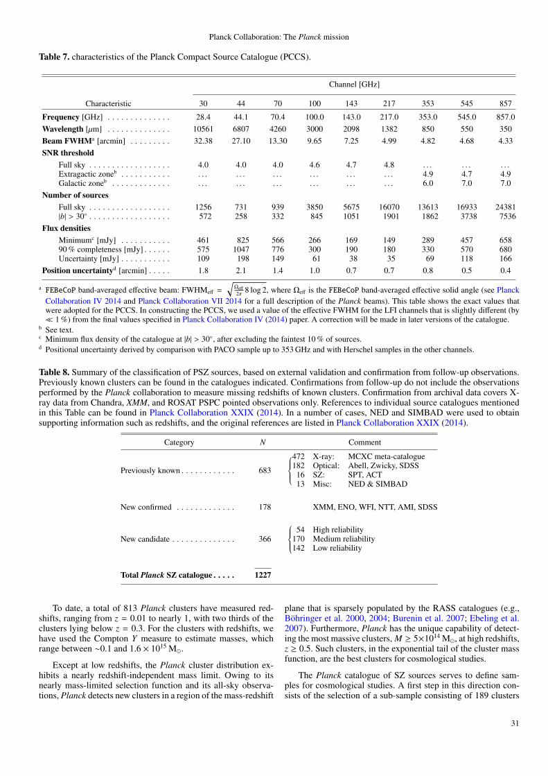
Planck Collaboration: The Planck mission
Table 7. characteristics of the Planck Compact Source Catalogue (PCCS).
Channel [GHz]
Characteristic 30 44 70 100 143 217 353 545 857
Frequency [GHz] . . . . . . . . . . . . . . 28.4 44.1 70.4 100.0 143.0 217.0 353.0 545.0 857.0Wavelength [µm] . . . . . . . . . . . . . . 10561 6807 4260 3000 2098 1382 850 550 350Beam FWHMa [arcmin] . . . . . . . . . 32.38 27.10 13.30 9.65 7.25 4.99 4.82 4.68 4.33SNR threshold
Full sky . . . . . . . . . . . . . . . . . . 4.0 4.0 4.0 4.6 4.7 4.8 . . . . . . . . .Extragactic zoneb . . . . . . . . . . . . . . . . . . . . . . . . . . . . . 4.9 4.7 4.9Galactic zoneb . . . . . . . . . . . . . . . . . . . . . . . . . . . . . . . 6.0 7.0 7.0
Number of sourcesFull sky . . . . . . . . . . . . . . . . . . 1256 731 939 3850 5675 16070 13613 16933 24381|b| > 30 . . . . . . . . . . . . . . . . . . 572 258 332 845 1051 1901 1862 3738 7536
Flux densitiesMinimumc [mJy] . . . . . . . . . . . 461 825 566 266 169 149 289 457 65890 % completeness [mJy] . . . . . . 575 1047 776 300 190 180 330 570 680Uncertainty [mJy] . . . . . . . . . . . 109 198 149 61 38 35 69 118 166
Position uncertaintyd [arcmin] . . . . . 1.8 2.1 1.4 1.0 0.7 0.7 0.8 0.5 0.4
a FEBeCoP band-averaged effective beam: FWHMeff =
√Ωeff
2π 8 log 2, where Ωeff is the FEBeCoP band-averaged effective solid angle (see PlanckCollaboration IV 2014 and Planck Collaboration VII 2014 for a full description of the Planck beams). This table shows the exact values thatwere adopted for the PCCS. In constructing the PCCS, we used a value of the effective FWHM for the LFI channels that is slightly different (by 1 %) from the final values specified in Planck Collaboration IV (2014) paper. A correction will be made in later versions of the catalogue.
b See text.c Minimum flux density of the catalogue at |b| > 30, after excluding the faintest 10 % of sources.d Positional uncertainty derived by comparison with PACO sample up to 353 GHz and with Herschel samples in the other channels.
Table 8. Summary of the classification of PSZ sources, based on external validation and confirmation from follow-up observations.Previously known clusters can be found in the catalogues indicated. Confirmations from follow-up do not include the observationsperformed by the Planck collaboration to measure missing redshifts of known clusters. Confirmation from archival data covers X-ray data from Chandra, XMM, and ROSAT PSPC pointed observations only. References to individual source catalogues mentionedin this Table can be found in Planck Collaboration XXIX (2014). In a number of cases, NED and SIMBAD were used to obtainsupporting information such as redshifts, and the original references are listed in Planck Collaboration XXIX (2014).
Category N Comment
Previously known . . . . . . . . . . . . 683
472 X-ray: MCXC meta-catalogue182 Optical: Abell, Zwicky, SDSS
16 SZ: SPT, ACT13 Misc: NED & SIMBAD
New confirmed . . . . . . . . . . . . . 178 XMM, ENO, WFI, NTT, AMI, SDSS
New candidate . . . . . . . . . . . . . . 366
54 High reliability
170 Medium reliability142 Low reliability
Total Planck SZ catalogue . . . . . 1227
To date, a total of 813 Planck clusters have measured red-shifts, ranging from z = 0.01 to nearly 1, with two thirds of theclusters lying below z = 0.3. For the clusters with redshifts, wehave used the Compton Y measure to estimate masses, whichrange between ∼0.1 and 1.6 × 10¹⁵ M.
Except at low redshifts, the Planck cluster distribution ex-hibits a nearly redshift-independent mass limit. Owing to itsnearly mass-limited selection function and its all-sky observa-tions, Planck detects new clusters in a region of the mass-redshift
plane that is sparsely populated by the RASS catalogues (e.g.,Bohringer et al. 2000, 2004; Burenin et al. 2007; Ebeling et al.2007). Furthermore, Planck has the unique capability of detect-ing the most massive clusters, M ≥ 5×10¹⁴ M, at high redshifts,z ≥ 0.5. Such clusters, in the exponential tail of the cluster massfunction, are the best clusters for cosmological studies.
The Planck catalogue of SZ sources serves to define sam-ples for cosmological studies. A first step in this direction con-sists of the selection of a sub-sample consisting of 189 clusters
31
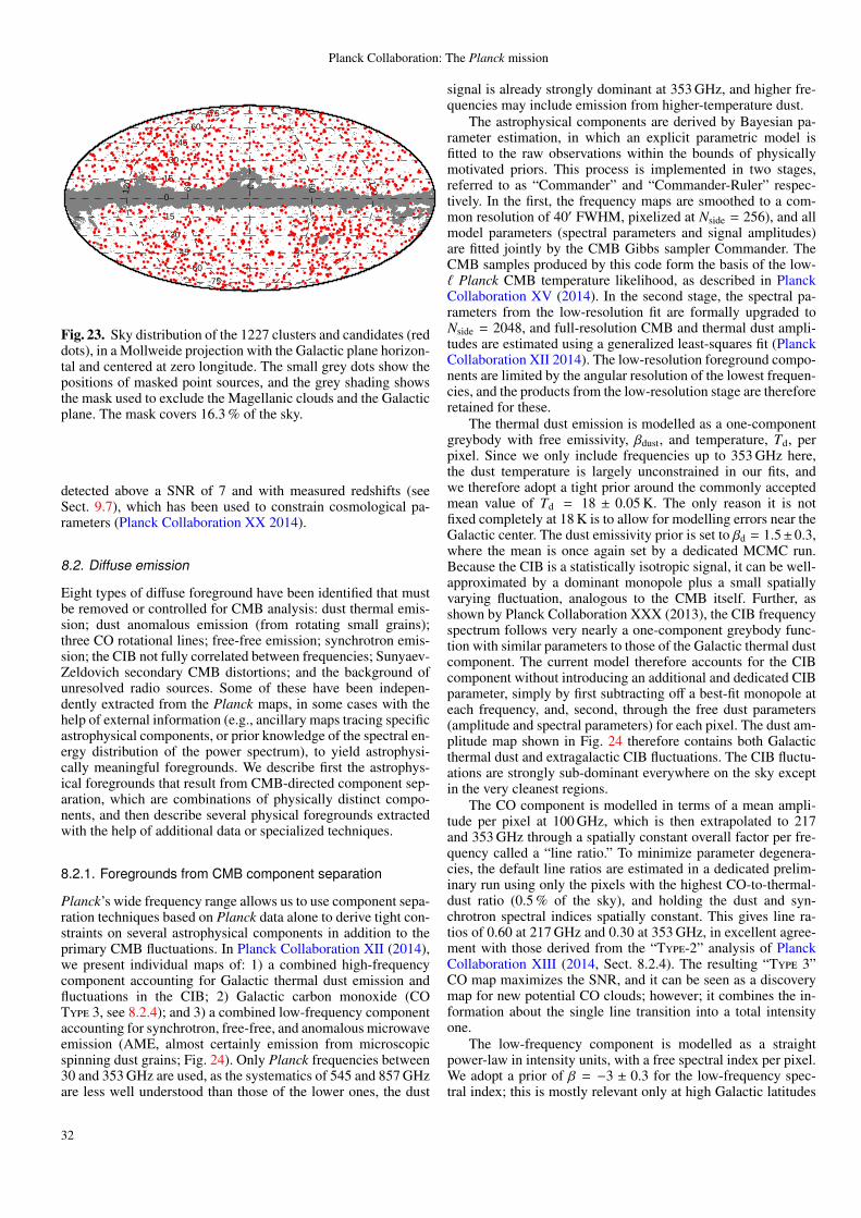
Planck Collaboration: The Planck mission
-120
-600
60120
-75-60
-45
-30
-15
0
15
30
4560
75
Fig. 23. Sky distribution of the 1227 clusters and candidates (reddots), in a Mollweide projection with the Galactic plane horizon-tal and centered at zero longitude. The small grey dots show thepositions of masked point sources, and the grey shading showsthe mask used to exclude the Magellanic clouds and the Galacticplane. The mask covers 16.3 % of the sky.
detected above a SNR of 7 and with measured redshifts (seeSect. 9.7), which has been used to constrain cosmological pa-rameters (Planck Collaboration XX 2014).
8.2. Diffuse emission
Eight types of diffuse foreground have been identified that mustbe removed or controlled for CMB analysis: dust thermal emis-sion; dust anomalous emission (from rotating small grains);three CO rotational lines; free-free emission; synchrotron emis-sion; the CIB not fully correlated between frequencies; Sunyaev-Zeldovich secondary CMB distortions; and the background ofunresolved radio sources. Some of these have been indepen-dently extracted from the Planck maps, in some cases with thehelp of external information (e.g., ancillary maps tracing specificastrophysical components, or prior knowledge of the spectral en-ergy distribution of the power spectrum), to yield astrophysi-cally meaningful foregrounds. We describe first the astrophys-ical foregrounds that result from CMB-directed component sep-aration, which are combinations of physically distinct compo-nents, and then describe several physical foregrounds extractedwith the help of additional data or specialized techniques.
8.2.1. Foregrounds from CMB component separation
Planck’s wide frequency range allows us to use component sepa-ration techniques based on Planck data alone to derive tight con-straints on several astrophysical components in addition to theprimary CMB fluctuations. In Planck Collaboration XII (2014),we present individual maps of: 1) a combined high-frequencycomponent accounting for Galactic thermal dust emission andfluctuations in the CIB; 2) Galactic carbon monoxide (COType 3, see 8.2.4); and 3) a combined low-frequency componentaccounting for synchrotron, free-free, and anomalous microwaveemission (AME, almost certainly emission from microscopicspinning dust grains; Fig. 24). Only Planck frequencies between30 and 353 GHz are used, as the systematics of 545 and 857 GHzare less well understood than those of the lower ones, the dust
signal is already strongly dominant at 353 GHz, and higher fre-quencies may include emission from higher-temperature dust.
The astrophysical components are derived by Bayesian pa-rameter estimation, in which an explicit parametric model isfitted to the raw observations within the bounds of physicallymotivated priors. This process is implemented in two stages,referred to as “Commander” and “Commander-Ruler” respec-tively. In the first, the frequency maps are smoothed to a com-mon resolution of 40′ FWHM, pixelized at Nside = 256), and allmodel parameters (spectral parameters and signal amplitudes)are fitted jointly by the CMB Gibbs sampler Commander. TheCMB samples produced by this code form the basis of the low-` Planck CMB temperature likelihood, as described in PlanckCollaboration XV (2014). In the second stage, the spectral pa-rameters from the low-resolution fit are formally upgraded toNside = 2048, and full-resolution CMB and thermal dust ampli-tudes are estimated using a generalized least-squares fit (PlanckCollaboration XII 2014). The low-resolution foreground compo-nents are limited by the angular resolution of the lowest frequen-cies, and the products from the low-resolution stage are thereforeretained for these.
The thermal dust emission is modelled as a one-componentgreybody with free emissivity, βdust, and temperature, Td, perpixel. Since we only include frequencies up to 353 GHz here,the dust temperature is largely unconstrained in our fits, andwe therefore adopt a tight prior around the commonly acceptedmean value of Td = 18 ± 0.05 K. The only reason it is notfixed completely at 18 K is to allow for modelling errors near theGalactic center. The dust emissivity prior is set to βd = 1.5±0.3,where the mean is once again set by a dedicated MCMC run.Because the CIB is a statistically isotropic signal, it can be well-approximated by a dominant monopole plus a small spatiallyvarying fluctuation, analogous to the CMB itself. Further, asshown by Planck Collaboration XXX (2013), the CIB frequencyspectrum follows very nearly a one-component greybody func-tion with similar parameters to those of the Galactic thermal dustcomponent. The current model therefore accounts for the CIBcomponent without introducing an additional and dedicated CIBparameter, simply by first subtracting off a best-fit monopole ateach frequency, and, second, through the free dust parameters(amplitude and spectral parameters) for each pixel. The dust am-plitude map shown in Fig. 24 therefore contains both Galacticthermal dust and extragalactic CIB fluctuations. The CIB fluctu-ations are strongly sub-dominant everywhere on the sky exceptin the very cleanest regions.
The CO component is modelled in terms of a mean ampli-tude per pixel at 100 GHz, which is then extrapolated to 217and 353 GHz through a spatially constant overall factor per fre-quency called a “line ratio.” To minimize parameter degenera-cies, the default line ratios are estimated in a dedicated prelim-inary run using only the pixels with the highest CO-to-thermal-dust ratio (0.5 % of the sky), and holding the dust and syn-chrotron spectral indices spatially constant. This gives line ra-tios of 0.60 at 217 GHz and 0.30 at 353 GHz, in excellent agree-ment with those derived from the “Type-2” analysis of PlanckCollaboration XIII (2014, Sect. 8.2.4). The resulting “Type 3”CO map maximizes the SNR, and it can be seen as a discoverymap for new potential CO clouds; however; it combines the in-formation about the single line transition into a total intensityone.
The low-frequency component is modelled as a straightpower-law in intensity units, with a free spectral index per pixel.We adopt a prior of β = −3 ± 0.3 for the low-frequency spec-tral index; this is mostly relevant only at high Galactic latitudes
32
Planck Collaboration: The Planck mission
where the SNR is low and the dominant foreground componentis expected to be synchrotron emission. In the signal-dominatedAME and free-free regions at low latitudes, the data are suffi-ciently strong that the prior becomes irrelevant. Figure 24 showsthe resulting component maps; Fig. 25 shows their frequencydependence at high latitudes.
In the 2013 data release, we adopt the posterior mean asour signal estimate, and the posterior RMS as the correspond-ing uncertainty. Mean and RMS maps are provided for each sig-nal component and for each per-pixel spectral parameter. Twocaveats are in order regarding use of these products for furtherscientific analysis. First, significant systematic uncertainties areassociated with several of these estimates. One example is thecorrelated HFI noise that is seen clearly in the thermal dust emis-sivity map; the products presented here do not take into accountspatially correlated noise. Second, the full posterior is signifi-cantly non-Gaussian due to the presence of non-Gaussian spec-tral parameters and the positivity amplitude prior, as well asstrongly correlated between components. The mean and RMSmaps provided in this data release should therefore be under-stood as a convenient representation of the full posterior, ratherthan a precise description of each component; if very high sta-tistical precision is required, one should use instead the originalensemble of individual Monte Carlo samples.
8.2.2. Thermal emission from Galactic dust
The CMB fades toward higher frequencies, whereas the thermaldust emission spectrum increases, and so dust becomes the dom-inant signal at submillimetre wavelengths. Planck has multifre-quency sensitivity in the “dust channels” covering the spectralrange where this transition occurs up to 857 GHz, for which theangular resolution is highest (Table 2). Dust emission is seenextending to high Galactic latitude in the wispy “cirrus” repre-sented in bluish tones in Fig. 1.
Understanding the frequency dependence and spatial fluctu-ations of the intensity and polarization from thermal dust is im-portant both in separating this foreground from the CMB and asan all-sky measure of column density. This has motivated thedevelopment of the Planck dust model (Planck CollaborationXI 2014; Fig. 22). The use of a range of available ancillarydata distinguishes this model from the dust component extractedusing component separation techniques and frequencies below353 GHz, described in Sect. 8.2.1.
The Planck dust model is based on the maps at 353, 545, and857 GHz, plus the IRAS 100 µm (3000 GHz) data from the IRISproduct (Miville-Deschenes & Lagache 2005). As described inPlanck Collaboration VI (2014), the zero level of these mapscan be set such that there is no dust emission where there is noatomic H i gas column density (according to the LAB survey,Kalberla et al. 2005).
The dust temperature Td is determined by multi-frequencyfitting of a greybody SED for optically thin thermal dust, Iν =τνBν(Td), where τν is the dust optical depth of the column of ma-terial and Bν(Td) is the Planck function for Td. In the Planck dustmodel there are three parameters, Td, τ353 at 353 GHz, and β, theexponent of the assumed power-law frequency dependence of τν.Conversion of τ353 to EB−V is established by correlating the sub-millimetre optical depth with SDSS reddening measurements ofquasars, a very similar approach to the one adopted by Schlegelet al. (1998).
All-sky maps of Td and τ from Planck were first presentedby Planck Collaboration XIX (2011) using a fixed β. In the newPlanck dust model (Planck Collaboration XI 2014), the maps
of Td and τ353 are at 5′ resolution, while β is estimated at 35′.This provides a much more detailed description of the thermaldust emission than the Finkbeiner et al. (1999) model, whichassumed constant β and used a Td map with an angular resolutionof several degrees.
The high resolution of Planck is a major improvement thatresults in a much more detailed mapping of column densitystructure, especially in denser regions of the ISM where the equi-librium temperature of big dust grains changes on small angularscales due to attenuation of the radiation field and also, it ap-pears, to changes in the intrinsic dust opacity and its ability toemit. Because of the increase in sensitivity, better control of sys-tematic effects, and the combination of four intensity maps at 5′resolution spanning the peak of the SED and into the Rayleigh-Jeans region, the new Planck EB−V product also provides a pre-cise estimate of the dust column density even in the diffuse ISMwhere Td does not vary as strongly on small scales.
8.2.3. Polarized emission from Galactic dust
As described in Sect. 1.3, Planck polarization data are in aless mature state than temperature data, especially at low mul-tipoles. Nevertheless, strong polarized synchrotron and thermaldust emission from the Galaxy can already be imaged with highsignificance. A first set of Galactic polarization papers will bepublished shortly. These papers will report results on the degreeof dust polarization (P/I) over the whole sky, comparisons withmaps of synchrotron polarization and Faraday rotation, the struc-ture of the Galactic magnetic field and its coupling with interstel-lar matter, as well as turbulence in the diffuse interstellar medium(ISM). With an angular resolution of 5′, the maps also reveal themagnetic field structure in molecular clouds and star forming re-gions, and can be used to study which grains contribute to theobserved polarization, where in the ISM they are aligned withthe Galactic magnetic field, and with what efficiency.
One highlight from these maps is the high degree of polar-ization of the dust emission from the diffuse interstellar medium,in many locations reaching P/I > 15 % at 353 GHz. These stud-ies will also address the statistics of P/I and φ for selected fieldstowards nearby molecular clouds (e.g., Fig. 26), the relationshipwith MHD simulations, the spectral dependence of the polarizedemission, and a comparison of the degree of polarization at sub-millimetre and visible (from stellar observations) wavelengths.
8.2.4. CO extraction
Rotational line emission from carbon monoxide (CO) inthe interstellar medium is present in all HFI bands except143 GHz, most significantly from the J=1→0 (115 GHz),J=2→1 (230 GHz), and J=3→2 (345 GHz) transitions. COemission arises from the denser parts of the interstellar medium,and is concentrated at low and intermediate Galactic latitudes.Three approaches to estimating CO emission have been evalu-ated and are described in Planck Collaboration XIII (2014).
Type 1 maps rely on the fact that each bolometer has a dif-ferent responsivity to CO, largely due to its specific bandpassshape. The transmission at the CO transition frequency has beenaccurately measured on the ground, and can also be estimatedby comparison to surveys made with dedicated observatories.Knowledge of the relative bolometer spectral response allowsextraction of each CO line independently of the others and ofany ancillary data. Being extracted from single-bolometer data,these maps have relatively low SNR; however, they are not af-
33
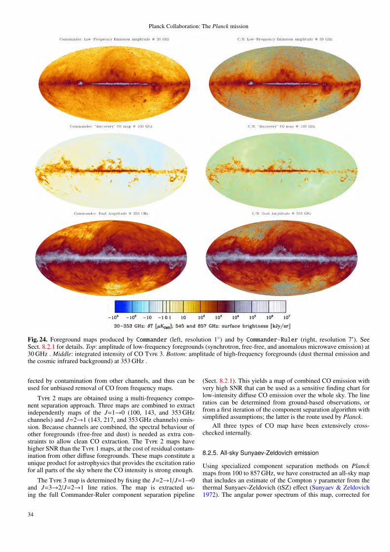
Planck Collaboration: The Planck mission
Fig. 24. Foreground maps produced by Commander (left, resolution 1) and by Commander-Ruler (right, resolution 7′). SeeSect. 8.2.1 for details. Top: amplitude of low-frequency foregrounds (synchrotron, free-free, and anomalous microwave emission) at30 GHz . Middle: integrated intensity of CO Type 3. Bottom: amplitude of high-frequency foregrounds (dust thermal emission andthe cosmic infrared background) at 353 GHz .
fected by contamination from other channels, and thus can beused for unbiased removal of CO from frequency maps.
Type 2 maps are obtained using a multi-frequency compo-nent separation approach. Three maps are combined to extractindependently maps of the J=1→0 (100, 143, and 353 GHzchannels) and J=2→1 (143, 217, and 353 GHz channels) emis-sion. Because channels are combined, the spectral behaviour ofother foregrounds (free-free and dust) is needed as extra con-straints to allow clean CO extraction. The Type 2 maps havehigher SNR than the Type 1 maps, at the cost of residual contam-ination from other diffuse foregrounds. These maps constitute aunique product for astrophysics that provides the excitation ratiofor all parts of the sky where the CO intensity is strong enough.
The Type 3 map is determined by fixing the J=2→1/J=1→0and J=3→2/J=2→1 line ratios. The map is extracted us-ing the full Commander-Ruler component separation pipeline
(Sect. 8.2.1). This yields a map of combined CO emission withvery high SNR that can be used as a sensitive finding chart forlow-intensity diffuse CO emission over the whole sky. The lineratios can be determined from ground-based observations, orfrom a first iteration of the component separation algorithm withsimplified assumptions; the latter is the route used by Planck.
All three types of CO map have been extensively cross-checked internally.
8.2.5. All-sky Sunyaev-Zeldovich emission
Using specialized component separation methods on Planckmaps from 100 to 857 GHz, we have constructed an all-sky mapthat includes an estimate of the Compton y parameter from thethermal Sunyaev-Zeldovich (tSZ) effect (Sunyaev & Zeldovich1972). The angular power spectrum of this map, corrected for
34
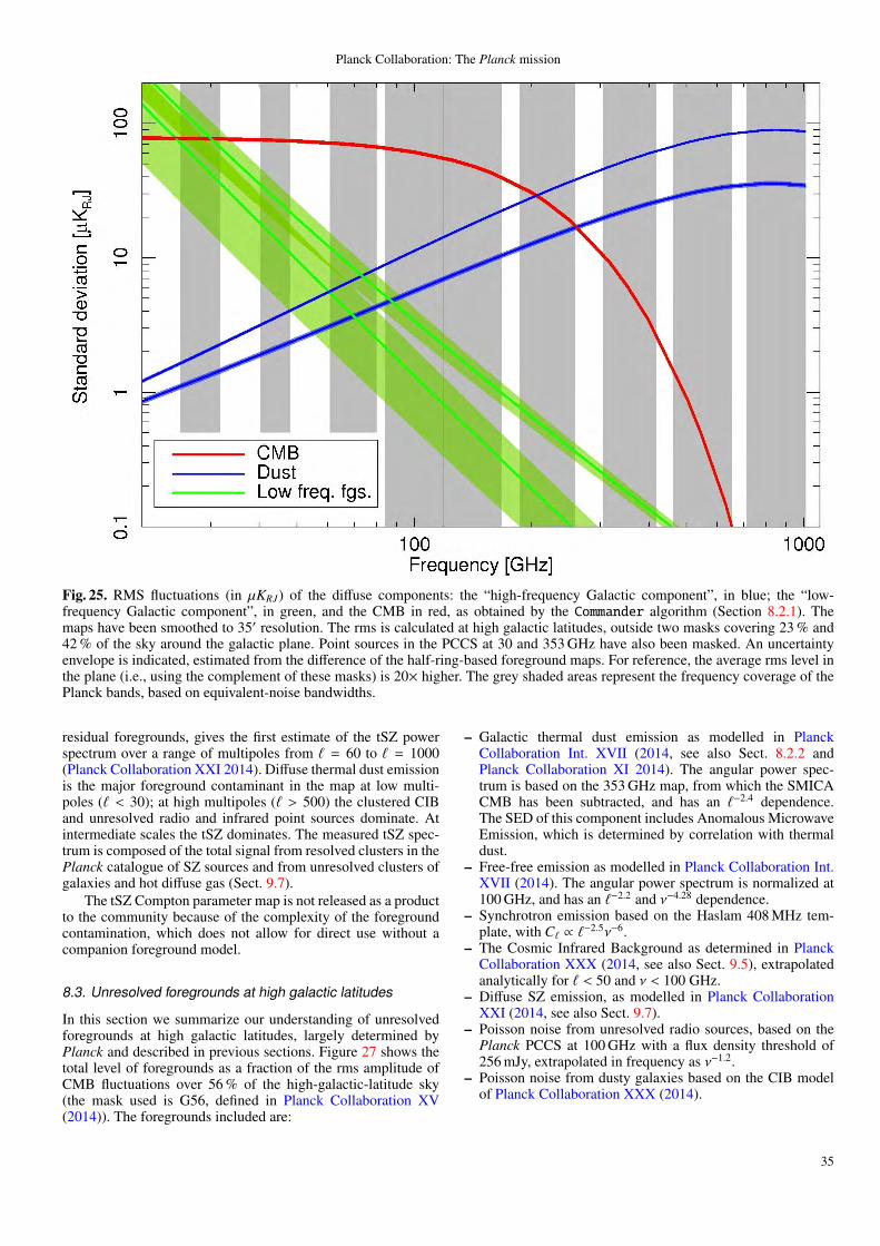
Planck Collaboration: The Planck mission
Fig. 25. RMS fluctuations (in µKRJ) of the diffuse components: the “high-frequency Galactic component”, in blue; the “low-frequency Galactic component”, in green, and the CMB in red, as obtained by the Commander algorithm (Section 8.2.1). Themaps have been smoothed to 35′ resolution. The rms is calculated at high galactic latitudes, outside two masks covering 23 % and42 % of the sky around the galactic plane. Point sources in the PCCS at 30 and 353 GHz have also been masked. An uncertaintyenvelope is indicated, estimated from the difference of the half-ring-based foreground maps. For reference, the average rms level inthe plane (i.e., using the complement of these masks) is 20× higher. The grey shaded areas represent the frequency coverage of thePlanck bands, based on equivalent-noise bandwidths.
residual foregrounds, gives the first estimate of the tSZ powerspectrum over a range of multipoles from ` = 60 to ` = 1000(Planck Collaboration XXI 2014). Diffuse thermal dust emissionis the major foreground contaminant in the map at low multi-poles (` < 30); at high multipoles (` > 500) the clustered CIBand unresolved radio and infrared point sources dominate. Atintermediate scales the tSZ dominates. The measured tSZ spec-trum is composed of the total signal from resolved clusters in thePlanck catalogue of SZ sources and from unresolved clusters ofgalaxies and hot diffuse gas (Sect. 9.7).
The tSZ Compton parameter map is not released as a productto the community because of the complexity of the foregroundcontamination, which does not allow for direct use without acompanion foreground model.
8.3. Unresolved foregrounds at high galactic latitudes
In this section we summarize our understanding of unresolvedforegrounds at high galactic latitudes, largely determined byPlanck and described in previous sections. Figure 27 shows thetotal level of foregrounds as a fraction of the rms amplitude ofCMB fluctuations over 56 % of the high-galactic-latitude sky(the mask used is G56, defined in Planck Collaboration XV(2014)). The foregrounds included are:
– Galactic thermal dust emission as modelled in PlanckCollaboration Int. XVII (2014, see also Sect. 8.2.2 andPlanck Collaboration XI 2014). The angular power spec-trum is based on the 353 GHz map, from which the SMICACMB has been subtracted, and has an `−2.4 dependence.The SED of this component includes Anomalous MicrowaveEmission, which is determined by correlation with thermaldust.
– Free-free emission as modelled in Planck Collaboration Int.XVII (2014). The angular power spectrum is normalized at100 GHz, and has an `−2.2 and ν−4.28 dependence.
– Synchrotron emission based on the Haslam 408 MHz tem-plate, with C` ∝ `−2.5ν−6.
– The Cosmic Infrared Background as determined in PlanckCollaboration XXX (2014, see also Sect. 9.5), extrapolatedanalytically for ` < 50 and ν < 100 GHz.
– Diffuse SZ emission, as modelled in Planck CollaborationXXI (2014, see also Sect. 9.7).
– Poisson noise from unresolved radio sources, based on thePlanck PCCS at 100 GHz with a flux density threshold of256 mJy, extrapolated in frequency as ν−1.2.
– Poisson noise from dusty galaxies based on the CIB modelof Planck Collaboration XXX (2014).
35
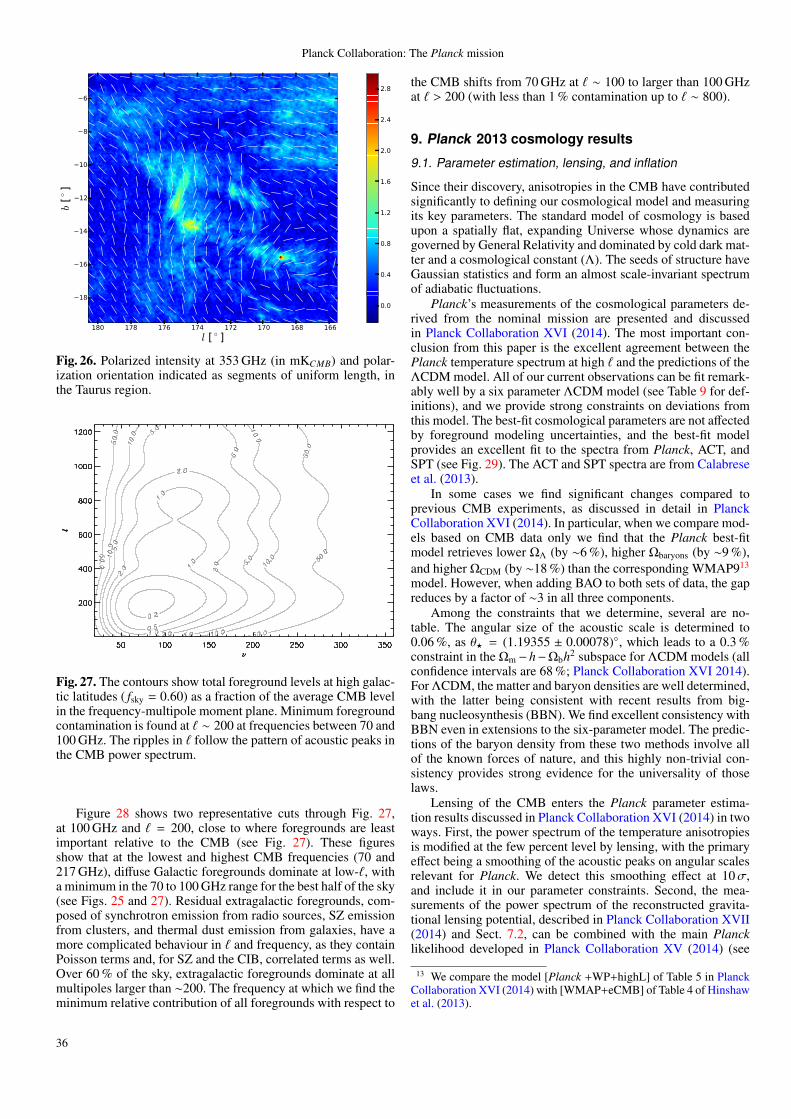
Planck Collaboration: The Planck mission
Fig. 26. Polarized intensity at 353 GHz (in mKCMB) and polar-ization orientation indicated as segments of uniform length, inthe Taurus region.
Fig. 27. The contours show total foreground levels at high galac-tic latitudes ( fsky = 0.60) as a fraction of the average CMB levelin the frequency-multipole moment plane. Minimum foregroundcontamination is found at ` ∼ 200 at frequencies between 70 and100 GHz. The ripples in ` follow the pattern of acoustic peaks inthe CMB power spectrum.
Figure 28 shows two representative cuts through Fig. 27,at 100 GHz and ` = 200, close to where foregrounds are leastimportant relative to the CMB (see Fig. 27). These figuresshow that at the lowest and highest CMB frequencies (70 and217 GHz), diffuse Galactic foregrounds dominate at low-`, witha minimum in the 70 to 100 GHz range for the best half of the sky(see Figs. 25 and 27). Residual extragalactic foregrounds, com-posed of synchrotron emission from radio sources, SZ emissionfrom clusters, and thermal dust emission from galaxies, have amore complicated behaviour in ` and frequency, as they containPoisson terms and, for SZ and the CIB, correlated terms as well.Over 60 % of the sky, extragalactic foregrounds dominate at allmultipoles larger than ∼200. The frequency at which we find theminimum relative contribution of all foregrounds with respect to
the CMB shifts from 70 GHz at ` ∼ 100 to larger than 100 GHzat ` > 200 (with less than 1 % contamination up to ` ∼ 800).
9. Planck 2013 cosmology results
9.1. Parameter estimation, lensing, and inflation
Since their discovery, anisotropies in the CMB have contributedsignificantly to defining our cosmological model and measuringits key parameters. The standard model of cosmology is basedupon a spatially flat, expanding Universe whose dynamics aregoverned by General Relativity and dominated by cold dark mat-ter and a cosmological constant (Λ). The seeds of structure haveGaussian statistics and form an almost scale-invariant spectrumof adiabatic fluctuations.
Planck’s measurements of the cosmological parameters de-rived from the nominal mission are presented and discussedin Planck Collaboration XVI (2014). The most important con-clusion from this paper is the excellent agreement between thePlanck temperature spectrum at high ` and the predictions of theΛCDM model. All of our current observations can be fit remark-ably well by a six parameter ΛCDM model (see Table 9 for def-initions), and we provide strong constraints on deviations fromthis model. The best-fit cosmological parameters are not affectedby foreground modeling uncertainties, and the best-fit modelprovides an excellent fit to the spectra from Planck, ACT, andSPT (see Fig. 29). The ACT and SPT spectra are from Calabreseet al. (2013).
In some cases we find significant changes compared toprevious CMB experiments, as discussed in detail in PlanckCollaboration XVI (2014). In particular, when we compare mod-els based on CMB data only we find that the Planck best-fitmodel retrieves lower ΩΛ (by ∼6 %), higher Ωbaryons (by ∼9 %),and higher ΩCDM (by ∼18 %) than the corresponding WMAP913
model. However, when adding BAO to both sets of data, the gapreduces by a factor of ∼3 in all three components.
Among the constraints that we determine, several are no-table. The angular size of the acoustic scale is determined to0.06 %, as θ? = (1.19355 ± 0.00078), which leads to a 0.3 %constraint in the Ωm − h−Ωbh2 subspace for ΛCDM models (allconfidence intervals are 68 %; Planck Collaboration XVI 2014).For ΛCDM, the matter and baryon densities are well determined,with the latter being consistent with recent results from big-bang nucleosynthesis (BBN). We find excellent consistency withBBN even in extensions to the six-parameter model. The predic-tions of the baryon density from these two methods involve allof the known forces of nature, and this highly non-trivial con-sistency provides strong evidence for the universality of thoselaws.
Lensing of the CMB enters the Planck parameter estima-tion results discussed in Planck Collaboration XVI (2014) in twoways. First, the power spectrum of the temperature anisotropiesis modified at the few percent level by lensing, with the primaryeffect being a smoothing of the acoustic peaks on angular scalesrelevant for Planck. We detect this smoothing effect at 10σ,and include it in our parameter constraints. Second, the mea-surements of the power spectrum of the reconstructed gravita-tional lensing potential, described in Planck Collaboration XVII(2014) and Sect. 7.2, can be combined with the main Plancklikelihood developed in Planck Collaboration XV (2014) (see
13 We compare the model [Planck +WP+highL] of Table 5 in PlanckCollaboration XVI (2014) with [WMAP+eCMB] of Table 4 of Hinshawet al. (2013).
36
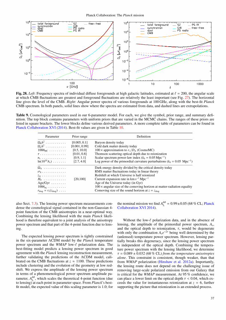
Planck Collaboration: The Planck mission
Fig. 28. Left: Frequency spectra of individual diffuse foregrounds at high galactic latitudes, estimated at ` = 200, the angular scaleat which CMB fluctuations are greatest and foreground fluctuations are relatively the least important (see Fig. 27). The horizontalline gives the level of the CMB. Right: Angular power spectra of various foregrounds at 100 GHz, along with the best-fit PlanckCMB spectrum. In both panels, solid lines show where the spectra are estimated from data, and dashed lines are extrapolations.
Table 9. Cosmological parameters used in our 6-parameter model. For each, we give the symbol, prior range, and summary defi-nition. The top block contains parameters with uniform priors that are varied in the MCMC chains. The ranges of these priors arelisted in square brackets. The lower blocks define various derived parameters. A more complete table of parameters can be found inPlanck Collaboration XVI (2014). Best-fit values are given in Table 10.
Parameter Prior range Definition
Ωbh2 . . . . . . . . . . . [0.005, 0.1] Baryon density todayΩch2 . . . . . . . . . . . [0.001, 0.99] Cold dark matter density today100θMC . . . . . . . . . [0.5, 10.0] 100× approximation to r∗/DA (CosmoMC)τ . . . . . . . . . . . . . . [0.01, 0.8] Thomson scattering optical depth due to reionizationns . . . . . . . . . . . . . [0.9, 1.1] Scalar spectrum power-law index (k0 = 0.05 Mpc−1)ln(1010As) . . . . . . . [2.7, 4.0] Log power of the primordial curvature perturbations (k0 = 0.05 Mpc−1)
ΩΛ . . . . . . . . . . . . Dark energy density divided by the critical density todayσ8 . . . . . . . . . . . . . RMS matter fluctuations today in linear theoryzre . . . . . . . . . . . . . Redshift at which Universe is half reionizedH0 . . . . . . . . . . . . [20,100] Current expansion rate in km s−1 Mpc−1
Age/Gyr . . . . . . . . Age of the Universe today (in Gyr)100θeq . . . . . . . . . . 100× angular size of the comoving horizon at matter-radiation equalityrdrag = rs(zdrag) . . . . Comoving size of the sound horizon at z = zdrag
also Sect. 7.3). The lensing power spectrum measurements con-dense the cosmological signal contained in the non-Gaussian 4-point function of the CMB anisotropies in a near-optimal way.Combining the lensing likelihood with the main Planck likeli-hood is therefore equivalent to a joint analysis of the anisotropypower spectrum and that part of the 4-point function due to lens-ing.
The expected lensing power spectrum is tightly constrainedin the six-parameter ΛCDM model by the Planck temperaturepower spectrum and the WMAP low-` polarization data. Thebest-fitting model predicts a lensing power spectrum in goodagreement with the Planck lensing reconstruction measurement,further validating the predictions of the ΛCDM model, cali-brated on the CMB fluctuations at z ≈ 1100. These predictionsinclude clustering and the evolution of the geometry at low red-shift. We express the amplitude of the lensing power spectrumin terms of a phenomenological power spectrum amplitude pa-rameter, Aφφ
L , which scales the theoretical 4-point function (dueto lensing) at each point in parameter space. From Planck’s best-fit model, the expected value of this scaling parameter is 1.0; for
the nominal mission we find AφφL = 0.99±0.05 (68 % CL; Planck
Collaboration XVI 2014).
Without the low-` polarization data, and in the absence oflensing, the amplitude of the primordial power spectrum, As,and the optical depth to reionization, τ, would be degeneratewith only the combination Ase−2τ being well determined by the(unlensed) temperature power spectrum. However, lensing par-tially breaks this degeneracy, since the lensing power spectrumis independent of the optical depth. Combining the tempera-ture power spectrum with the lensing likelihood, we determineτ = 0.089 ± 0.032 (68 % CL) from the temperature anisotropiesalone. This constraint is consistent, though weaker, than thatfrom WMAP polarization (Hinshaw et al. 2012a). Importantly,the lensing route does not depend on the challenging issue ofremoving large-scale polarized emission from our Galaxy thatis critical for the WMAP measurement. At 95 % confidence, wecan place a lower limit on the optical depth τ < 0.04, which ex-ceeds the value for instantaneous reionization at z = 6, furthersupporting the picture that reionization is an extended process.
37
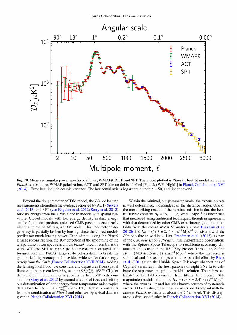
Planck Collaboration: The Planck mission
2 10 50
102
103
104
D `[µ
K2 ]
90 18
500 1000 1500 2000 2500 3000
Multipole moment, `
Planck
WMAP9
ACT
SPT
1 0.2 0.1 0.06Angular scale
Fig. 29. Measured angular power spectra of Planck, WMAP9, ACT, and SPT. The model plotted is Planck’s best-fit model includingPlanck temperature, WMAP polarization, ACT, and SPT (the model is labelled [Planck+WP+HighL] in Planck Collaboration XVI(2014)). Error bars include cosmic variance. The horizontal axis is logarithmic up to ` = 50, and linear beyond.
Beyond the six-parameter ΛCDM model, the Planck lensingmeasurements strengthen the evidence reported by ACT (Sieverset al. 2013) and SPT (van Engelen et al. 2012; Story et al. 2012)for dark energy from the CMB alone in models with spatial cur-vature. Closed models with low energy density in dark energycan be found that produce unlensed CMB power spectra nearlyidentical to the best-fitting ΛCDM model. This “geometric” de-generacy is partially broken by lensing, since the closed modelspredict too much lensing power. Even without using the Plancklensing reconstruction, the 10σ detection of the smoothing of thetemperature power spectrum allows Planck, used in combinationwith ACT and SPT at high-` (to better constrain extragalacticforegrounds) and WMAP large scale polarization, to break thegeometrical degeneracy, and provides evidence for dark energypurely from the CMB (Planck Collaboration XVII 2014). Addingthe lensing likelihood, we constrain any departures from spatialflatness at the percent level: ΩK = −0.0096+0.010
−0.0082 (68 % CL) forthe same data combination, improving earlier CMB-only con-straints (Story et al. 2012) by around a factor of two, and settingour determination of dark energy from temperature anisotropiesdata alone to ΩΛ = 0.67+0.027
−0.023 (68 % CL). Tighter constraintsfrom the combination of Planck and other astrophysical data aregiven in Planck Collaboration XVI (2014).
Within the minimal, six-parameter model the expansion rateis well determined, independent of the distance ladder. One ofthe most striking results of the nominal mission is that the best-fit Hubble constant H0 = (67 ± 1.2) km s−1 Mpc−1, is lower thanthat measured using traditional techniques, though in agreementwith that determined by other CMB experiments (e.g., most no-tably from the recent WMAP9 analysis where Hinshaw et al.2012b find H0 = (69.7 ± 2.4) km s−1 Mpc−1 consistent with thePlanck value to within ∼ 1σ). Freedman et al. (2012), as partof the Carnegie Hubble Program, use mid-infrared observationswith the Spitzer Space Telescope to recalibrate secondary dis-tance methods used in the HST Key Project. These authors findH0 = (74.3 ± 1.5 ± 2.1) km s−1 Mpc−1 where the first error isstatistical and the second systematic. A parallel effort by Riesset al. (2011) used the Hubble Space Telescope observations ofCepheid variables in the host galaxies of eight SNe Ia to cali-brate the supernova magnitude-redshift relation. Their ‘best es-timate’ of the Hubble constant, from fitting the calibrated SNemagnitude-redshift relation is, H0 = (73.8 ± 2.4) km s−1 Mpc−1
where the error is 1σ and includes known sources of systematicerrors. At face value, these measurements are discrepant with thecurrent Planck estimate at about the 2.5σ level. This discrep-ancy is discussed further in Planck Collaboration XVI (2014).
38
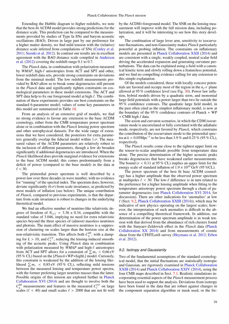
Planck Collaboration: The Planck mission
Extending the Hubble diagram to higher redshifts, we notethat the best-fit ΛCDM model provides strong predictions for thedistance scale. This prediction can be compared to the measure-ments provided by studies of Type Ia SNe and baryon acousticoscillations (BAO). Driven in large part by our preference fora higher matter density, we find mild tension with the (relative)distance scale inferred from compilations of SNe (Conley et al.2011; Suzuki et al. 2012). In contrast our results are in excellentagreement with the BAO distance scale compiled in Andersonet al. (2012) covering the redshift range 0.1 to 0.7.
The Planck data, in combination with polarization measuredby WMAP, high-` anisotropies from ACT and SPT and other,lower redshift data sets, provide strong constraints on deviationsfrom the minimal model. The low redshift measurements pro-vided by BAO allow us to break some degeneracies still presentin the Planck data and significantly tighten constraints on cos-mological parameters in these model extensions. The ACT andSPT data help to fix our foreground model at high `. The combi-nation of these experiments provides our best constraints on thestandard 6-parameter model; values of some key parameters inthis model are summarized in Table 10.
From an analysis of an extensive grid of models, we findno strong evidence to favour any extension to the base ΛCDMcosmology, either from the CMB temperature power spectrumalone or in combination with the Planck lensing power spectrumand other astrophysical datasets. For the wide range of exten-sions that we have considered, the posteriors for extra parame-ters generally overlap the fiducial model within 1σ. The mea-sured values of the ΛCDM parameters are relatively robust tothe inclusion of different parameters, though a few do broadensignificantly if additional degeneracies are introduced. When thePlanck likelihood does provide marginal evidence for extensionsto the base ΛCDM model, this comes predominantly from adeficit of power (compared to the base model) in the data at` < 30.
The primordial power spectrum is well described by apower-law over three decades in wave number, with no evidencefor “running” of the spectral index. The spectrum does, however,deviate significantly (6σ) from scale invariance, as predicted bymost models of inflation (see below). The unique contributionof Planck, compared to previous experiments, is that the depar-ture from scale invariance is robust to changes in the underlyingtheoretical model.
We find an effective number of neutrino-like relativistic de-grees of freedom of Ne f f = 3.36 ± 0.34, compatible with thestandard value of 3.046, implying no need for extra relativisticspecies beyond the three species of (almost) massless neutrinosand photons. The main effect of massive neutrinos is a suppres-sion of clustering on scales larger than the horizon size at thenon-relativisitic transition. This affects both Cφφ
L , with a damp-ing for L > 10, and CTT
` , reducing the lensing-induced smooth-ing of the acoustic peaks. Using Planck data in combinationwith polarization measured by WMAP and high-` anisotropiesfrom ACT and SPT allows for a constraint of
∑mν < 0.66 eV
(95 % CL) based on the [Planck+WP+highL] model. Curiously,this constraint is weakened by the addition of the lensing like-lihood
∑mν < 0.85 eV (95 % CL), reflecting mild tensions
between the measured lensing and temperature power spectra,with the former preferring larger neutrino masses than the latter.Possible origins of this tension are explored further in PlanckCollaboration XVI (2014) and are thought to involve both theCφφ
L measurements and features in the measured CTT` on large
scales (` < 40) and small scales ` > 2000 that are not fit well
by the ΛCDM+foreground model. The SNR on the lensing mea-surement will improve with the full mission data, including po-larization, and it will be interesting to see how this story devel-ops.
The combination of large lever arm, sensitivity to isocurva-ture fluctuations, and non-Gaussianity makes Planck particularlypowerful at probing inflation. The constraints on inflationarymodels are presented in Planck Collaboration XXII (2014) andare consistent with a single, weakly coupled, neutral scalar fielddriving the accelerated expansion and generating curvature per-turbations. The data can be explained using a field with a canon-ical kinetic term and slowly rolling down a featureless potential,and we find no compelling evidence calling for any extension tothis simple explanation.
Of the models considered, those with locally concave poten-tials are favored and occupy most of the region in the ns-r planeallowed at 95 % confidence level (see Fig. 30). Power law infla-tion, hybrid models driven by a quadratic term, and monomiallarge field potentials with a power larger than two lie outside the95 % confidence contours. The quadratic large field model, inthe past often cited as the simplest inflationary model, is now atthe boundary of the 95 % confidence contours of Planck + WP+ CMB high ` data.
The axion and curvaton scenarios, in which the CDM isocur-vature mode is uncorrelated or fully correlated with the adiabaticmode, respectively, are not favored by Planck, which constrainsthe contribution of the isocurvature mode to the primordial spec-tra at k = 0.05Mpc−1 to be less than 3.9 % and 0.25 % (95 % CL),respectively.
The Planck results come close to the tightest upper limit onthe tensor-to-scalar amplitude possible from temperature dataalone. The precise determination of the higher acoustic peaksbreaks degeneracies that have weakened earlier measurements.The bound (r < 0.11 at 95 % CL) implies an upper limit for theenergy scale of standard inflation of 1.9 × 10¹⁶ GeV (95 %CL).
The power spectrum of the best fit base ΛCDM cosmol-ogy has a higher amplitude than the observed power spectrumat multipoles ` < 30. The low-` difference is in turn related tothe preference for a higher lensing amplitude when fitting to thetemperature anisotropy power spectrum through a chain of pa-rameter degeneracies (see Planck Collaboration XVI 2014, fordiscussion). There are other indications for ‘anomalies’ at low` (Sect. 9.2, Planck Collaboration XXIII (2014)), which may beindicative of new physics operating on the largest scales; how-ever, the interpretation of such anomalies is difficult in the ab-sence of a compelling theoretical framework. In addition, ourdetermination of the power spectrum amplitude is in weak ten-sion with that derived from the abundance of rich clusters foundwith the Sunyaev-Zeldovich effect in the Planck data (PlanckCollaboration XX 2014) and from measurements of cosmicshear from the CFHTLenS survey (Heymans et al. 2012; Erbenet al. 2012).
9.2. Isotropy and Gaussianity
Two of the fundamental assumptions of the standard cosmolog-ical model, that the initial fluctuations are statistically isotropicand Gaussian, are rigorously examined in Planck CollaborationXXIII (2014) and Planck Collaboration XXIV (2014), using thefour CMB maps described in Sect. 7.1. Realistic simulations in-corporating essential aspects of the Planck measurement processhave been used to support the analysis. Deviations from isotropyhave been found in the data that are robust against changes inthe component separation algorithm or mask used, or the fre-
39
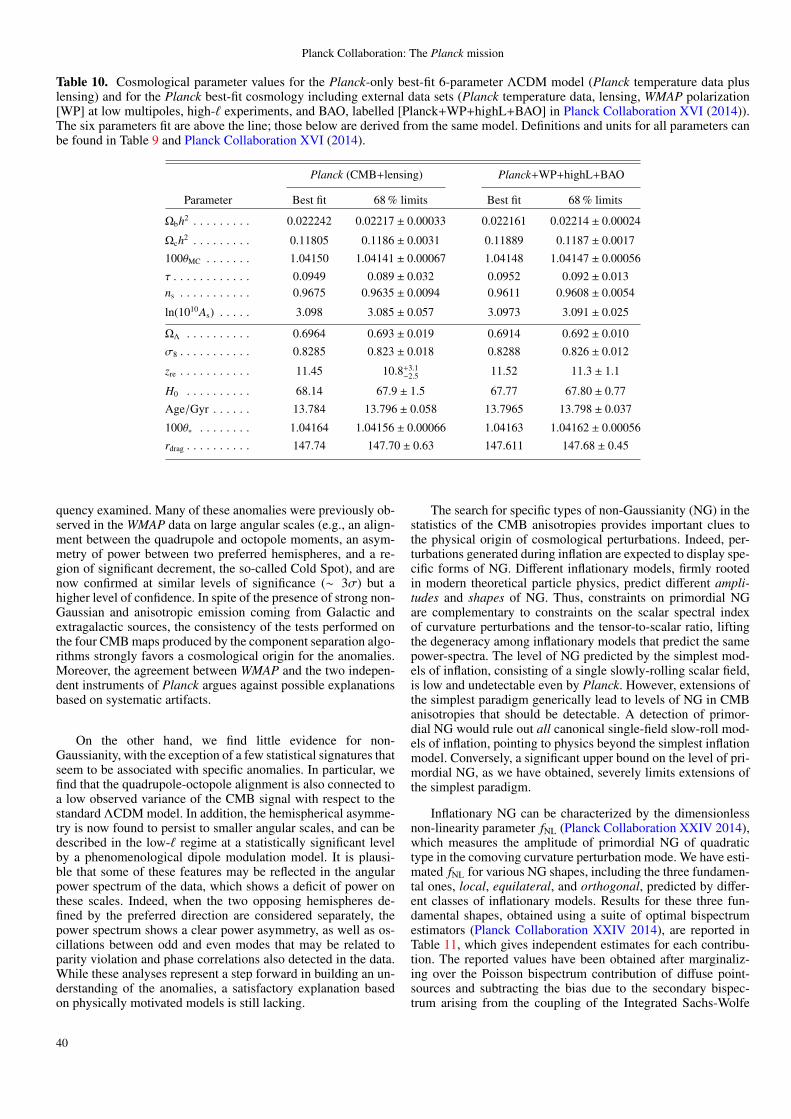
Planck Collaboration: The Planck mission
Table 10. Cosmological parameter values for the Planck-only best-fit 6-parameter ΛCDM model (Planck temperature data pluslensing) and for the Planck best-fit cosmology including external data sets (Planck temperature data, lensing, WMAP polarization[WP] at low multipoles, high-` experiments, and BAO, labelled [Planck+WP+highL+BAO] in Planck Collaboration XVI (2014)).The six parameters fit are above the line; those below are derived from the same model. Definitions and units for all parameters canbe found in Table 9 and Planck Collaboration XVI (2014).
Planck (CMB+lensing) Planck+WP+highL+BAO
Parameter Best fit 68 % limits Best fit 68 % limits
Ωbh2 . . . . . . . . . 0.022242 0.02217 ± 0.00033 0.022161 0.02214 ± 0.00024
Ωch2 . . . . . . . . . 0.11805 0.1186 ± 0.0031 0.11889 0.1187 ± 0.0017100θMC . . . . . . . 1.04150 1.04141 ± 0.00067 1.04148 1.04147 ± 0.00056
τ . . . . . . . . . . . . 0.0949 0.089 ± 0.032 0.0952 0.092 ± 0.013ns . . . . . . . . . . . 0.9675 0.9635 ± 0.0094 0.9611 0.9608 ± 0.0054
ln(1010As) . . . . . 3.098 3.085 ± 0.057 3.0973 3.091 ± 0.025
ΩΛ . . . . . . . . . . 0.6964 0.693 ± 0.019 0.6914 0.692 ± 0.010σ8 . . . . . . . . . . . 0.8285 0.823 ± 0.018 0.8288 0.826 ± 0.012
zre . . . . . . . . . . . 11.45 10.8+3.1−2.5 11.52 11.3 ± 1.1
H0 . . . . . . . . . . 68.14 67.9 ± 1.5 67.77 67.80 ± 0.77
Age/Gyr . . . . . . 13.784 13.796 ± 0.058 13.7965 13.798 ± 0.037
100θ∗ . . . . . . . . 1.04164 1.04156 ± 0.00066 1.04163 1.04162 ± 0.00056rdrag . . . . . . . . . . 147.74 147.70 ± 0.63 147.611 147.68 ± 0.45
quency examined. Many of these anomalies were previously ob-served in the WMAP data on large angular scales (e.g., an align-ment between the quadrupole and octopole moments, an asym-metry of power between two preferred hemispheres, and a re-gion of significant decrement, the so-called Cold Spot), and arenow confirmed at similar levels of significance (∼ 3σ) but ahigher level of confidence. In spite of the presence of strong non-Gaussian and anisotropic emission coming from Galactic andextragalactic sources, the consistency of the tests performed onthe four CMB maps produced by the component separation algo-rithms strongly favors a cosmological origin for the anomalies.Moreover, the agreement between WMAP and the two indepen-dent instruments of Planck argues against possible explanationsbased on systematic artifacts.
On the other hand, we find little evidence for non-Gaussianity, with the exception of a few statistical signatures thatseem to be associated with specific anomalies. In particular, wefind that the quadrupole-octopole alignment is also connected toa low observed variance of the CMB signal with respect to thestandard ΛCDM model. In addition, the hemispherical asymme-try is now found to persist to smaller angular scales, and can bedescribed in the low-` regime at a statistically significant levelby a phenomenological dipole modulation model. It is plausi-ble that some of these features may be reflected in the angularpower spectrum of the data, which shows a deficit of power onthese scales. Indeed, when the two opposing hemispheres de-fined by the preferred direction are considered separately, thepower spectrum shows a clear power asymmetry, as well as os-cillations between odd and even modes that may be related toparity violation and phase correlations also detected in the data.While these analyses represent a step forward in building an un-derstanding of the anomalies, a satisfactory explanation basedon physically motivated models is still lacking.
The search for specific types of non-Gaussianity (NG) in thestatistics of the CMB anisotropies provides important clues tothe physical origin of cosmological perturbations. Indeed, per-turbations generated during inflation are expected to display spe-cific forms of NG. Different inflationary models, firmly rootedin modern theoretical particle physics, predict different ampli-tudes and shapes of NG. Thus, constraints on primordial NGare complementary to constraints on the scalar spectral indexof curvature perturbations and the tensor-to-scalar ratio, liftingthe degeneracy among inflationary models that predict the samepower-spectra. The level of NG predicted by the simplest mod-els of inflation, consisting of a single slowly-rolling scalar field,is low and undetectable even by Planck. However, extensions ofthe simplest paradigm generically lead to levels of NG in CMBanisotropies that should be detectable. A detection of primor-dial NG would rule out all canonical single-field slow-roll mod-els of inflation, pointing to physics beyond the simplest inflationmodel. Conversely, a significant upper bound on the level of pri-mordial NG, as we have obtained, severely limits extensions ofthe simplest paradigm.
Inflationary NG can be characterized by the dimensionlessnon-linearity parameter fNL (Planck Collaboration XXIV 2014),which measures the amplitude of primordial NG of quadratictype in the comoving curvature perturbation mode. We have esti-mated fNL for various NG shapes, including the three fundamen-tal ones, local, equilateral, and orthogonal, predicted by differ-ent classes of inflationary models. Results for these three fun-damental shapes, obtained using a suite of optimal bispectrumestimators (Planck Collaboration XXIV 2014), are reported inTable 11, which gives independent estimates for each contribu-tion. The reported values have been obtained after marginaliz-ing over the Poisson bispectrum contribution of diffuse point-sources and subtracting the bias due to the secondary bispec-trum arising from the coupling of the Integrated Sachs-Wolfe
40
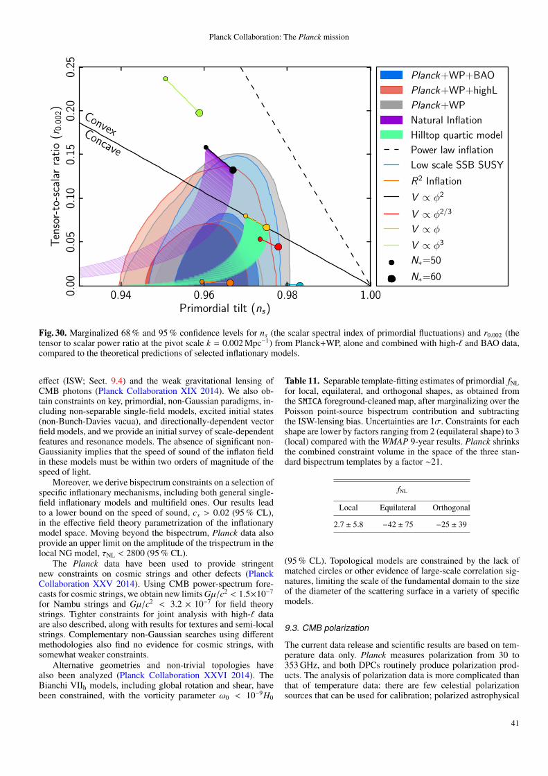
Planck Collaboration: The Planck mission
0.94 0.96 0.98 1.00Primordial tilt (ns)
0.00
0.05
0.10
0.15
0.20
0.25
Ten
sor-
to-s
cala
rra
tio
(r0.
002)
ConvexConcave
Planck+WP+BAO
Planck+WP+highL
Planck+WP
Natural Inflation
Hilltop quartic model
Power law inflation
Low scale SSB SUSY
R2 Inflation
V ∝ φ2
V ∝ φ2/3
V ∝ φ
V ∝ φ3
N∗=50
N∗=60
Fig. 30. Marginalized 68 % and 95 % confidence levels for ns (the scalar spectral index of primordial fluctuations) and r0.002 (thetensor to scalar power ratio at the pivot scale k = 0.002 Mpc−1) from Planck+WP, alone and combined with high-` and BAO data,compared to the theoretical predictions of selected inflationary models.
effect (ISW; Sect. 9.4) and the weak gravitational lensing ofCMB photons (Planck Collaboration XIX 2014). We also ob-tain constraints on key, primordial, non-Gaussian paradigms, in-cluding non-separable single-field models, excited initial states(non-Bunch-Davies vacua), and directionally-dependent vectorfield models, and we provide an initial survey of scale-dependentfeatures and resonance models. The absence of significant non-Gaussianity implies that the speed of sound of the inflaton fieldin these models must be within two orders of magnitude of thespeed of light.
Moreover, we derive bispectrum constraints on a selection ofspecific inflationary mechanisms, including both general single-field inflationary models and multifield ones. Our results leadto a lower bound on the speed of sound, cs > 0.02 (95 % CL),in the effective field theory parametrization of the inflationarymodel space. Moving beyond the bispectrum, Planck data alsoprovide an upper limit on the amplitude of the trispectrum in thelocal NG model, τNL < 2800 (95 % CL).
The Planck data have been used to provide stringentnew constraints on cosmic strings and other defects (PlanckCollaboration XXV 2014). Using CMB power-spectrum fore-casts for cosmic strings, we obtain new limits Gµ/c2 < 1.5×10⁻⁷
for Nambu strings and Gµ/c2 < 3.2 × 10⁻⁷ for field theorystrings. Tighter constraints for joint analysis with high-` dataare also described, along with results for textures and semi-localstrings. Complementary non-Gaussian searches using differentmethodologies also find no evidence for cosmic strings, withsomewhat weaker constraints.
Alternative geometries and non-trivial topologies havealso been analyzed (Planck Collaboration XXVI 2014). TheBianchi VIIh models, including global rotation and shear, havebeen constrained, with the vorticity parameter ω0 < 10−9H0
Table 11. Separable template-fitting estimates of primordial fNLfor local, equilateral, and orthogonal shapes, as obtained fromthe SMICA foreground-cleaned map, after marginalizing over thePoisson point-source bispectrum contribution and subtractingthe ISW-lensing bias. Uncertainties are 1σ. Constraints for eachshape are lower by factors ranging from 2 (equilateral shape) to 3(local) compared with the WMAP 9-year results. Planck shrinksthe combined constraint volume in the space of the three stan-dard bispectrum templates by a factor ∼21.
fNL
Local Equilateral Orthogonal
2.7 ± 5.8 −42 ± 75 −25 ± 39
(95 % CL). Topological models are constrained by the lack ofmatched circles or other evidence of large-scale correlation sig-natures, limiting the scale of the fundamental domain to the sizeof the diameter of the scattering surface in a variety of specificmodels.
9.3. CMB polarization
The current data release and scientific results are based on tem-perature data only. Planck measures polarization from 30 to353 GHz, and both DPCs routinely produce polarization prod-ucts. The analysis of polarization data is more complicated thanthat of temperature data: there are few celestial polarizationsources that can be used for calibration; polarized astrophysical
41
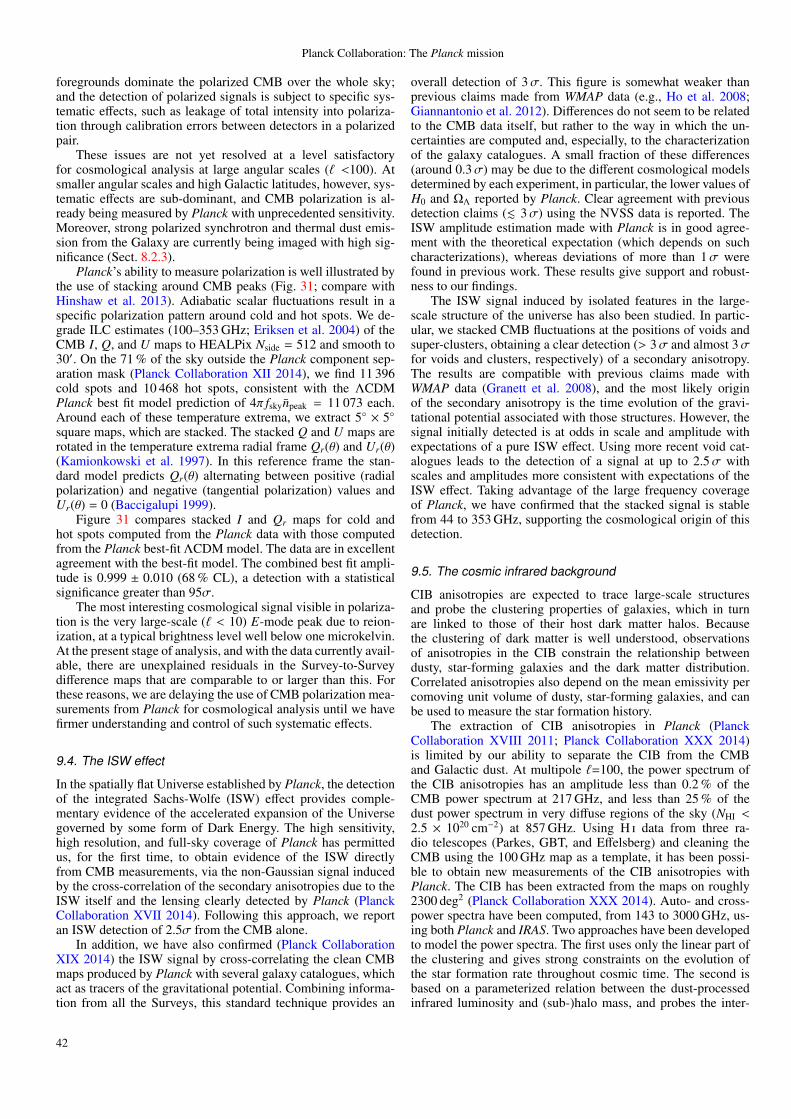
Planck Collaboration: The Planck mission
foregrounds dominate the polarized CMB over the whole sky;and the detection of polarized signals is subject to specific sys-tematic effects, such as leakage of total intensity into polariza-tion through calibration errors between detectors in a polarizedpair.
These issues are not yet resolved at a level satisfactoryfor cosmological analysis at large angular scales (` <100). Atsmaller angular scales and high Galactic latitudes, however, sys-tematic effects are sub-dominant, and CMB polarization is al-ready being measured by Planck with unprecedented sensitivity.Moreover, strong polarized synchrotron and thermal dust emis-sion from the Galaxy are currently being imaged with high sig-nificance (Sect. 8.2.3).
Planck’s ability to measure polarization is well illustrated bythe use of stacking around CMB peaks (Fig. 31; compare withHinshaw et al. 2013). Adiabatic scalar fluctuations result in aspecific polarization pattern around cold and hot spots. We de-grade ILC estimates (100–353 GHz; Eriksen et al. 2004) of theCMB I, Q, and U maps to HEALPix Nside = 512 and smooth to30′. On the 71 % of the sky outside the Planck component sep-aration mask (Planck Collaboration XII 2014), we find 11 396cold spots and 10 468 hot spots, consistent with the ΛCDMPlanck best fit model prediction of 4π fskynpeak = 11 073 each.Around each of these temperature extrema, we extract 5 × 5square maps, which are stacked. The stacked Q and U maps arerotated in the temperature extrema radial frame Qr(θ) and Ur(θ)(Kamionkowski et al. 1997). In this reference frame the stan-dard model predicts Qr(θ) alternating between positive (radialpolarization) and negative (tangential polarization) values andUr(θ) = 0 (Baccigalupi 1999).
Figure 31 compares stacked I and Qr maps for cold andhot spots computed from the Planck data with those computedfrom the Planck best-fit ΛCDM model. The data are in excellentagreement with the best-fit model. The combined best fit ampli-tude is 0.999 ± 0.010 (68 % CL), a detection with a statisticalsignificance greater than 95σ.
The most interesting cosmological signal visible in polariza-tion is the very large-scale (` < 10) E-mode peak due to reion-ization, at a typical brightness level well below one microkelvin.At the present stage of analysis, and with the data currently avail-able, there are unexplained residuals in the Survey-to-Surveydifference maps that are comparable to or larger than this. Forthese reasons, we are delaying the use of CMB polarization mea-surements from Planck for cosmological analysis until we havefirmer understanding and control of such systematic effects.
9.4. The ISW effect
In the spatially flat Universe established by Planck, the detectionof the integrated Sachs-Wolfe (ISW) effect provides comple-mentary evidence of the accelerated expansion of the Universegoverned by some form of Dark Energy. The high sensitivity,high resolution, and full-sky coverage of Planck has permittedus, for the first time, to obtain evidence of the ISW directlyfrom CMB measurements, via the non-Gaussian signal inducedby the cross-correlation of the secondary anisotropies due to theISW itself and the lensing clearly detected by Planck (PlanckCollaboration XVII 2014). Following this approach, we reportan ISW detection of 2.5σ from the CMB alone.
In addition, we have also confirmed (Planck CollaborationXIX 2014) the ISW signal by cross-correlating the clean CMBmaps produced by Planck with several galaxy catalogues, whichact as tracers of the gravitational potential. Combining informa-tion from all the Surveys, this standard technique provides an
overall detection of 3σ. This figure is somewhat weaker thanprevious claims made from WMAP data (e.g., Ho et al. 2008;Giannantonio et al. 2012). Differences do not seem to be relatedto the CMB data itself, but rather to the way in which the un-certainties are computed and, especially, to the characterizationof the galaxy catalogues. A small fraction of these differences(around 0.3σ) may be due to the different cosmological modelsdetermined by each experiment, in particular, the lower values ofH0 and ΩΛ reported by Planck. Clear agreement with previousdetection claims (. 3σ) using the NVSS data is reported. TheISW amplitude estimation made with Planck is in good agree-ment with the theoretical expectation (which depends on suchcharacterizations), whereas deviations of more than 1σ werefound in previous work. These results give support and robust-ness to our findings.
The ISW signal induced by isolated features in the large-scale structure of the universe has also been studied. In partic-ular, we stacked CMB fluctuations at the positions of voids andsuper-clusters, obtaining a clear detection (> 3σ and almost 3σfor voids and clusters, respectively) of a secondary anisotropy.The results are compatible with previous claims made withWMAP data (Granett et al. 2008), and the most likely originof the secondary anisotropy is the time evolution of the gravi-tational potential associated with those structures. However, thesignal initially detected is at odds in scale and amplitude withexpectations of a pure ISW effect. Using more recent void cat-alogues leads to the detection of a signal at up to 2.5σ withscales and amplitudes more consistent with expectations of theISW effect. Taking advantage of the large frequency coverageof Planck, we have confirmed that the stacked signal is stablefrom 44 to 353 GHz, supporting the cosmological origin of thisdetection.
9.5. The cosmic infrared background
CIB anisotropies are expected to trace large-scale structuresand probe the clustering properties of galaxies, which in turnare linked to those of their host dark matter halos. Becausethe clustering of dark matter is well understood, observationsof anisotropies in the CIB constrain the relationship betweendusty, star-forming galaxies and the dark matter distribution.Correlated anisotropies also depend on the mean emissivity percomoving unit volume of dusty, star-forming galaxies, and canbe used to measure the star formation history.
The extraction of CIB anisotropies in Planck (PlanckCollaboration XVIII 2011; Planck Collaboration XXX 2014)is limited by our ability to separate the CIB from the CMBand Galactic dust. At multipole `=100, the power spectrum ofthe CIB anisotropies has an amplitude less than 0.2 % of theCMB power spectrum at 217 GHz, and less than 25 % of thedust power spectrum in very diffuse regions of the sky (NHI <2.5 × 1020 cm−2) at 857 GHz. Using H i data from three ra-dio telescopes (Parkes, GBT, and Effelsberg) and cleaning theCMB using the 100 GHz map as a template, it has been possi-ble to obtain new measurements of the CIB anisotropies withPlanck. The CIB has been extracted from the maps on roughly2300 deg2 (Planck Collaboration XXX 2014). Auto- and cross-power spectra have been computed, from 143 to 3000 GHz, us-ing both Planck and IRAS. Two approaches have been developedto model the power spectra. The first uses only the linear part ofthe clustering and gives strong constraints on the evolution ofthe star formation rate throughout cosmic time. The second isbased on a parameterized relation between the dust-processedinfrared luminosity and (sub-)halo mass, and probes the inter-
42
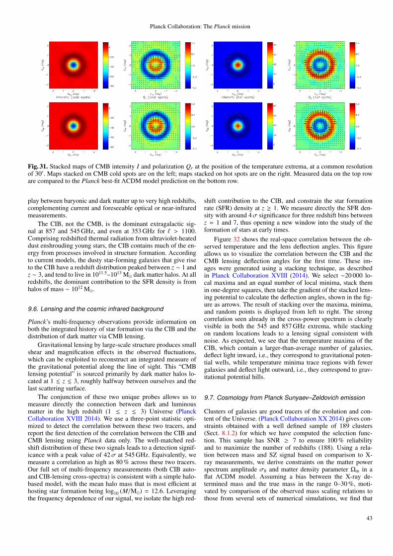
Planck Collaboration: The Planck mission
Fig. 31. Stacked maps of CMB intensity I and polarization Qr at the position of the temperature extrema, at a common resolutionof 30′. Maps stacked on CMB cold spots are on the left; maps stacked on hot spots are on the right. Measured data on the top roware compared to the Planck best-fit ΛCDM model prediction on the bottom row.
play between baryonic and dark matter up to very high redshifts,complementing current and foreseeable optical or near-infraredmeasurements.
The CIB, not the CMB, is the dominant extragalactic sig-nal at 857 and 545 GHz, and even at 353 GHz for ` > 1100.Comprising redshifted thermal radiation from ultraviolet-heateddust enshrouding young stars, the CIB contains much of the en-ergy from processes involved in structure formation. Accordingto current models, the dusty star-forming galaxies that give riseto the CIB have a redshift distribution peaked between z ∼ 1 andz ∼ 3, and tend to live in 1011.5–1013 M dark matter halos. At allredshifts, the dominant contribution to the SFR density is fromhalos of mass ∼ 1012 M.
9.6. Lensing and the cosmic infrared background
Planck’s multi-frequency observations provide information onboth the integrated history of star formation via the CIB and thedistribution of dark matter via CMB lensing.
Gravitational lensing by large-scale structure produces smallshear and magnification effects in the observed fluctuations,which can be exploited to reconstruct an integrated measure ofthe gravitational potential along the line of sight. This “CMBlensing potential” is sourced primarily by dark matter halos lo-cated at 1 . z . 3, roughly halfway between ourselves and thelast scattering surface.
The conjunction of these two unique probes allows us tomeasure directly the connection between dark and luminousmatter in the high redshift (1 ≤ z ≤ 3) Universe (PlanckCollaboration XVIII 2014). We use a three-point statistic opti-mized to detect the correlation between these two tracers, andreport the first detection of the correlation between the CIB andCMB lensing using Planck data only. The well-matched red-shift distribution of these two signals leads to a detection signif-icance with a peak value of 42σ at 545 GHz. Equivalently, wemeasure a correlation as high as 80 % across these two tracers.Our full set of multi-frequency measurements (both CIB auto-and CIB-lensing cross-spectra) is consistent with a simple halo-based model, with the mean halo mass that is most efficient athosting star formation being log10 (M/M) = 12.6. Leveragingthe frequency dependence of our signal, we isolate the high red-
shift contribution to the CIB, and constrain the star formationrate (SFR) density at z ≥ 1. We measure directly the SFR den-sity with around 4σ significance for three redshift bins betweenz = 1 and 7, thus opening a new window into the study of theformation of stars at early times.
Figure 32 shows the real-space correlation between the ob-served temperature and the lens deflection angles. This figureallows us to visualize the correlation between the CIB and theCMB lensing deflection angles for the first time. These im-ages were generated using a stacking technique, as describedin Planck Collaboration XVIII (2014). We select ∼20 000 lo-cal maxima and an equal number of local minima, stack themin one-degree squares, then take the gradient of the stacked lens-ing potential to calculate the deflection angles, shown in the fig-ure as arrows. The result of stacking over the maxima, minima,and random points is displayed from left to right. The strongcorrelation seen already in the cross-power spectrum is clearlyvisible in both the 545 and 857 GHz extrema, while stackingon random locations leads to a lensing signal consistent withnoise. As expected, we see that the temperature maxima of theCIB, which contain a larger-than-average number of galaxies,deflect light inward, i.e., they correspond to gravitational poten-tial wells, while temperature minima trace regions with fewergalaxies and deflect light outward, i.e., they correspond to grav-itational potential hills.
9.7. Cosmology from Planck Sunyaev–Zeldovich emission
Clusters of galaxies are good tracers of the evolution and con-tent of the Universe. (Planck Collaboration XX 2014) gives con-straints obtained with a well defined sample of 189 clusters(Sect. 8.1.2) for which we have computed the selection func-tion. This sample has SNR ≥ 7 to ensure 100 % reliabilityand to maximize the number of redshifts (188). Using a rela-tion between mass and SZ signal based on comparison to X-ray measurements, we derive constraints on the matter powerspectrum amplitude σ8 and matter density parameter Ωm in aflat ΛCDM model. Assuming a bias between the X-ray de-termined mass and the true mass in the range 0–30 %, moti-vated by comparison of the observed mass scaling relations tothose from several sets of numerical simulations, we find that
43
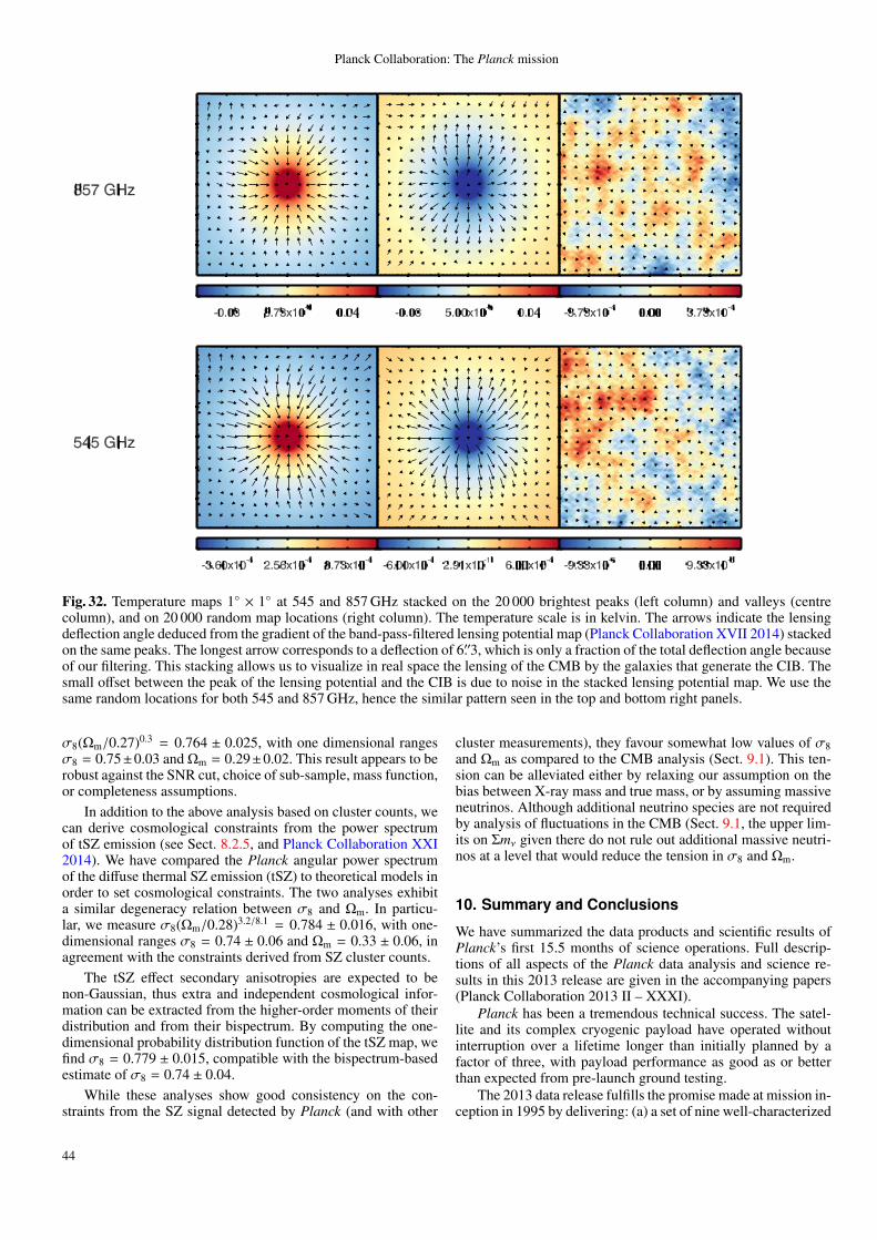
Planck Collaboration: The Planck mission
Fig. 32. Temperature maps 1 × 1 at 545 and 857 GHz stacked on the 20 000 brightest peaks (left column) and valleys (centrecolumn), and on 20 000 random map locations (right column). The temperature scale is in kelvin. The arrows indicate the lensingdeflection angle deduced from the gradient of the band-pass-filtered lensing potential map (Planck Collaboration XVII 2014) stackedon the same peaks. The longest arrow corresponds to a deflection of 6.′′3, which is only a fraction of the total deflection angle becauseof our filtering. This stacking allows us to visualize in real space the lensing of the CMB by the galaxies that generate the CIB. Thesmall offset between the peak of the lensing potential and the CIB is due to noise in the stacked lensing potential map. We use thesame random locations for both 545 and 857 GHz, hence the similar pattern seen in the top and bottom right panels.
σ8(Ωm/0.27)0.3 = 0.764 ± 0.025, with one dimensional rangesσ8 = 0.75±0.03 and Ωm = 0.29±0.02. This result appears to berobust against the SNR cut, choice of sub-sample, mass function,or completeness assumptions.
In addition to the above analysis based on cluster counts, wecan derive cosmological constraints from the power spectrumof tSZ emission (see Sect. 8.2.5, and Planck Collaboration XXI2014). We have compared the Planck angular power spectrumof the diffuse thermal SZ emission (tSZ) to theoretical models inorder to set cosmological constraints. The two analyses exhibita similar degeneracy relation between σ8 and Ωm. In particu-lar, we measure σ8(Ωm/0.28)3.2/8.1 = 0.784 ± 0.016, with one-dimensional ranges σ8 = 0.74 ± 0.06 and Ωm = 0.33 ± 0.06, inagreement with the constraints derived from SZ cluster counts.
The tSZ effect secondary anisotropies are expected to benon-Gaussian, thus extra and independent cosmological infor-mation can be extracted from the higher-order moments of theirdistribution and from their bispectrum. By computing the one-dimensional probability distribution function of the tSZ map, wefind σ8 = 0.779 ± 0.015, compatible with the bispectrum-basedestimate of σ8 = 0.74 ± 0.04.
While these analyses show good consistency on the con-straints from the SZ signal detected by Planck (and with other
cluster measurements), they favour somewhat low values of σ8and Ωm as compared to the CMB analysis (Sect. 9.1). This ten-sion can be alleviated either by relaxing our assumption on thebias between X-ray mass and true mass, or by assuming massiveneutrinos. Although additional neutrino species are not requiredby analysis of fluctuations in the CMB (Sect. 9.1, the upper lim-its on Σmν given there do not rule out additional massive neutri-nos at a level that would reduce the tension in σ8 and Ωm.
10. Summary and Conclusions
We have summarized the data products and scientific results ofPlanck’s first 15.5 months of science operations. Full descrip-tions of all aspects of the Planck data analysis and science re-sults in this 2013 release are given in the accompanying papers(Planck Collaboration 2013 II – XXXI).
Planck has been a tremendous technical success. The satel-lite and its complex cryogenic payload have operated withoutinterruption over a lifetime longer than initially planned by afactor of three, with payload performance as good as or betterthan expected from pre-launch ground testing.
The 2013 data release fulfills the promise made at mission in-ception in 1995 by delivering: (a) a set of nine well-characterized
44
Planck Collaboration: The Planck mission
frequency maps with sub-percent calibration accuracy across theCMB channels; (b) a map of the temperature anisotropies of theCMB limited only by unresolved foregrounds down to an an-gular resolution of 5′; (c) a catalogue of compact Galactic andextragalactic sources that represents an important improvementover the Early Release Compact Source Catalogue released inJanuary 2011; (d) a catalogue of galaxy clusters detected via theSunyaev-Zeldovich effect, which increases by a factor of ∼10the number of clusters detected by this technique; and (e) a first-generation set of maps of diffuse foregrounds that includes themain sources of Galactic emission — thermal dust and the cos-mic infrared background at high frequencies and synchrotron,free-free, and anomalous emission at low frequencies.
In addition to these long-planned products, the 2013 releaseincludes: an all-sky map of dust opacity that represents an impor-tant improvement over the best previous IRAS-based product; anall-sky map of the CMB lensing deflection field, the first everin its category; all-sky maps of the integrated emission of car-bon monoxide, an important tracer of the interstellar medium;and the first measurement of the angular power spectrum of thediffuse Sunyaev-Zeldovich emission over a large part of the sky.
The main cosmological results of Planck can be summarisedas follows:
– Using a likelihood approach that combines Planck CMB andlensing data, data from ACT and SPT at high `s to constrainforegrounds, and the WMAP polarized likelihood functionat low `s to constrain τ, we have estimated the values of asix-parameter ΛCDM model with the highest accuracy ever.These estimates are highly robust, as demonstrated by theuse of multiple methods based both on likelihood and oncomponent-separated maps.
– The parameters of the Planck 6-parameter ΛCDM modelare significantly different from those previously estimated.In particular, we find a weaker cosmological constant (by∼2 %), more baryons (by ∼3 %), and more cold dark matter(by ∼5 %). The spectral index of primordial fluctuations isfirmly established to be below unity, even when extendingthe ΛCDM model with additional parameters.
– We find no significant improvements to the best-fit modelwhen extending the set of parameters beyond six, implyingno need for new physics to explain the Planck measurements.
– The Planck best-fit model is in excellent agreement with themost current BAO data. However, it requires a Hubble con-stant that is significantly lower (∼67 km s−1 Mpc−1) than thatdetermined from traditional measurement techniques, rais-ing the possibility of systematic effects in the latter.
– An exploration of parameter space beyond the basic set leadsto: (a) establishing a value for the effective number of rela-tivistic species (neutrinos) consistent with the standard valueof 3.046; (b) constraining the flatness of space-time to alevel of 0.1% (including BAO data); and (c) setting signif-icantly improved constraints on the total mass of neutrinos(at∑
mν < 0.85 eV), the abundance of primordial helium,and the running of the spectral index of the power spectrum(Planck Collaboration XVI 2014).
– We find no evidence at the current level of analysis fortensor modes, for a dynamical form of dark energy, orfor time-variations of the fine structure constant (PlanckCollaboration XVI 2014).
– We find some tension between the amplitude of matter fluc-tuations (σ8) derived from CMB data and that derived fromSunyaev-Zeldovich data; we attribute this tension to uncer-
tainties in cluster physics and measurements that affect thelatter.
– We find important support for single-field slow-roll inflationvia our constraints on running of the spectral index, curva-ture, and fNL.
– The Planck data squeeze the region of allowed standard in-flationary models, preferring a concave potential. Power lawinflation, the simplest hybrid inflationary models, and simplemonomial models with n > 2, do not provide a good fit to thedata.
– We find no evidence for statistical deviations from isotropy at` > 600, to very high precision Planck Collaboration XXIII(2014).
– We do find evidence for deviations from isotropy at lowmultipoles, confirming the existence of the so-called WMAPanomalies, the hemispheric asymmetry and the Cold Spot.
– We find a coherent deficit of power at multipoles between 20and 30 with respect to our best-fit ΛCDM model.
These results highlight the maturity and precision beingachieved in our understanding of the Universe, but at the sametime reveal small differences between the data and the best-fitmodel whose significance is not yet fully understood.
Other results for which the current Planck data are makingunique contributions are:
– A 25σ detection of the distortion of the CMB due to lensingby intervening structure yields a highly significant map overmost of the sky of the integrated distribution of mass back tothe CMB surface of last scattering. The detection of lensinghelps Planck to break parameter degeneracies, in particularto constrain the reionization optical depth without the helpof polarization data.
– The first detection at high significance (42σ) of the cross-correlation between CMB lensing and the cosmic infraredbackground, which allows us to constrain the star formationrate at high redshifts.
– The measurement of the angular power spectrum of the cos-mic infrared background over a large area and at frequenciesas low as 217 GHz, which allows us to constrain the proper-ties of dark matter halos at high redshifts.
– The first power spectrum of the diffuse Sunyaev-Zeldovichemission over the range 60 ≤ ` ≤ 1000, used to constrain theamplitude of matter fluctuations (σ8).
– A 2.5σ detection of the Integrated Sachs-Wolfe effect viaits cross-correlation with Planck-detected lensing, providingindependent evidence for ΩΛ ∼0.7.
The Planck 2013 release does not include polarization prod-ucts. Our current cosmological analysis relies not at all onPlanck polarization data, and only mildly on WMAP polariza-tion data. However, we have shown that quite basic processingof the CMB polarization already yields angular power spectrain excellent agreement with the Planck best-fit cosmology de-rived from temperature data only. Analysis of the stacking of hotand cold CMB peaks shows spectacular agreement with expec-tations, and demonstrates the potential of the Planck’s CMB po-larization measurements. A number of papers on polarized dustemission are due to be published within a few months. All thesepoints show that the processing of Planck polarization data iswell advanced, and progressing towards the goal of releasing po-larized data and associated results in 2014.
Acknowledgements. Planck is too large a project to allow full acknowledgementof all contributions by individuals, institutions, industries, and funding agen-cies. The main entities involved in the mission operations are as follows. The
45
Planck Collaboration: The Planck mission
European Space Agency operates the satellite via its Mission Operations Centrelocated at ESOC (Darmstadt, Germany) and coordinates scientific operationsvia the Planck Science Office located at ESAC (Madrid, Spain). Two Consortia,comprising around 100 scientific institutes within Europe, the USA, and Canada,and funded by agencies from the participating countries, developed the scien-tific instruments LFI and HFI, and continue to operate them via InstrumentOperations Teams located in Trieste (Italy) and Orsay (France). The Consortiaare also responsible for scientific processing of the acquired data. The Consortiaare led by the Principal Investigators: J.-L. Puget in France for HFI (funded prin-cipally by CNES and CNRS/INSU-IN2P3) and N. Mandolesi in Italy for LFI(funded principally via ASI). NASA’s US Planck Project, based at JPL and in-volving scientists at many US institutions, contributes significantly to the effortsof these two Consortia. A third Consortium, led by H. U. Norgaard-Nielsen andsupported by the Danish Natural Research Council, contributed to the reflec-tor programme. The author list for this paper has been selected by the PlanckScience Team from the Planck Collaboration, and is composed of individualsfrom all of the above entities who have made multi-year contributions to the de-velopment of the mission. It does not pretend to be inclusive of all contributionsto Planck. A description of the Planck Collaboration and a list of its members, in-dicating which technical or scientific activities they have been involved in, can befound at (http://www.rssd.esa.int/index.php?project=PLANCK& page=PlanckCollaboration). The Planck Collaboration acknowledges the support of: ESA;CNES, and CNRS/INSU-IN2P3-INP (France); ASI, CNR, and INAF (Italy);NASA and DoE (USA); STFC and UKSA (UK); CSIC, MICINN, and JA(Spain); Tekes, AoF, and CSC (Finland); DLR and MPG (Germany); CSA(Canada); DTU Space (Denmark); SER/SSO (Switzerland); RCN (Norway); SFI(Ireland); FCT/MCTES (Portugal); and PRACE (EU).
ReferencesAnderson, L., Aubourg, E., Bailey, S., et al. 2012, MNRAS, 427, 3435Baccigalupi, C. 1999, Phys. Rev. D, 59, 123004Bennett, C. L., Halpern, M., Hinshaw, G., et al. 2003, ApJS, 148, 1Bennett, C. L., Larson, D., Weiland, J. L., et al. 2013, ApJS, 208, 20Bersanelli, M., Mandolesi, N., Butler, R. C., et al. 2010, A&A, 520, A4Bohringer, H., Schuecker, P., Guzzo, L., et al. 2004, A&A, 425, 367Bohringer, H., Voges, W., Huchra, J. P., et al. 2000, ApJS, 129, 435Burenin, R. A., Vikhlinin, A., Hornstrup, A., et al. 2007, ApJS, 172, 561Calabrese, E., Hlozek, R. A., Battaglia, N., et al. 2013, ArXiv e-printsCardoso, J., Martin, M., Delabrouille, J., Betoule, M., & Patanchon, G. 2008,
IEEE Journal of Selected Topics in Signal Processing, 2, 735, special issueon Signal Processing for Astronomical and Space Research Applications
Chen, X., Rachen, J. P., Lopez-Caniego, M., et al. 2013, A&A, 553, A107Condon, J. J., Cotton, W. D., Greisen, E. W., et al. 1998, AJ, 115, 1693Conley, A., Guy, J., Sullivan, M., et al. 2011, ApJS, 192, 1Delabrouille, J., Betoule, M., Melin, J.-B., et al. 2012, ArXiv e-printsDelabrouille, J., Cardoso, J., Le Jeune, M., et al. 2009, A&A, 493, 835Delabrouille, J., Cardoso, J.-F., & Patanchon, G. 2003, MNRAS, 346, 1089Dunkley, J., Calabrese, E., Sievers, J., et al. 2013, ArXiv e-printsDunkley, J., Hlozek, R., Sievers, J., et al. 2011, ApJ, 739, 52Eales, S., Dunne, L., Clements, D., et al. 2010, PASP, 122, 499Ebeling, H., Barrett, E., Donovan, D., et al. 2007, ApJ, 661, L33Erben, T., Hildebrandt, H., Miller, L., et al. 2012, ArXiv e-printsEriksen, H. K., Banday, A. J., Gorski, K. M., & Lilje, P. B. 2004, ApJ, 612, 633Eriksen, H. K., Dickinson, C., Lawrence, C. R., et al. 2006, ApJ, 641, 665Eriksen, H. K., Jewell, J. B., Dickinson, C., et al. 2008, ApJ, 676, 10Fernandez-Cobos, R., Vielva, P., Barreiro, R. B., & Martınez-Gonzalez, E. 2012,
MNRAS, 420, 2162Finkbeiner, D. P., Davis, M., & Schlegel, D. J. 1999, ApJ, 524, 867Fixsen, D. J. 2009, ApJ, 707, 916Fraisse, A. A., Ade, P. A. R., Amiri, M., et al. 2011, ArXiv e-printsFreedman, W. L., Madore, B. F., Scowcroft, V., et al. 2012, ApJ, 758, 24Giannantonio, T., Crittenden, R., Nichol, R., & Ross, A. J. 2012, MNRAS, 426,
2581Gonzalez-Nuevo, J., Argueso, F., Lopez-Caniego, M., et al. 2006, MNRAS, 369,
1603Gorski, K. M., Hivon, E., Banday, A. J., et al. 2005, ApJ, 622, 759Granett, B. R., Neyrinck, M. C., & Szapudi, I. 2008, ApJ, 683, L99Griffin, M. J., Abergel, A., Abreu, A., et al. 2010, A&A, 518, L3Healey, S. E., Romani, R. W., Taylor, G. B., et al. 2007, ApJS, 171, 61Herranz, D., Lopez-Caniego, M., Sanz, J. L., & Gonzalez-Nuevo, J. 2009,
MNRAS, 394, 510Herranz, D. & Sanz, J. L. 2008, IEEE Journal of Selected Topics in Signal
Processing, 2, 727Heymans, C., Van Waerbeke, L., Miller, L., et al. 2012, MNRAS, 427, 146Hinshaw, G., Larson, D., Komatsu, E., et al. 2013, ApJS, 208, 19Hinshaw, G., Larson, D., Komatsu, E., et al. 2012a, ArXiv e-prints
Hinshaw, G., Larson, D., Komatsu, E., et al. 2012b, ArXiv e-printsHinshaw, G., Weiland, J. L., Hill, R. S., et al. 2009, ApJS, 180, 225Ho, S., Hirata, C., Padmanabhan, N., Seljak, U., & Bahcall, N. 2008,
Phys. Rev. D, 78, 043519Jarosik, N., Bennett, C. L., Dunkley, J., et al. 2011, ApJS, 192, 14Kalberla, P. M. W., Burton, W. B., Hartmann, D., et al. 2005, A&A, 440, 775Kamionkowski, M., Kosowsky, A., & Stebbins, A. 1997, Phys. Rev. D, 55, 7368Keihanen, E., Keskitalo, R., Kurki-Suonio, H., Poutanen, T., & Sirvio, A. 2010,
A&A, 510, A57Keisler, R., Reichardt, C. L., Aird, K. A., et al. 2011, ApJ, 743, 28Kelsall, T., Weiland, J. L., Franz, B. A., et al. 1998, ApJ, 508, 44Koester, B. et al. 2007, Astrophys.J., 660, 239Kosowsky, A. 2003, New A Rev., 47, 939Kurinsky, N., Sajina, A., Partridge, B., et al. 2013, A&A, 549, A133Lamarre, J., Puget, J., Ade, P. A. R., et al. 2010, A&A, 520, A9Lopez-Caniego, M., Gonzalez-Nuevo, J., Herranz, D., et al. 2007, ApJS, 170,
108Lopez-Caniego, M., Herranz, D., Gonzalez-Nuevo, J., et al. 2006, MNRAS, 370,
2047Massardi, M., Lopez-Caniego, M., Gonzalez-Nuevo, J., et al. 2009, MNRAS,
392, 733Mather, J. C., Fixsen, D. J., Shafer, R. A., Mosier, C., & Wilkinson, D. T. 1999,
ApJ, 512, 511Mennella, A., Butler, R. C., Curto, A., et al. 2011, A&A, 536, A3Mitra, S., Rocha, G., Gorski, K. M., et al. 2011, ApJS, 193, 5Miville-Deschenes, M.-A. & Lagache, G. 2005, ApJS, 157, 302Murphy, T., Sadler, E. M., Ekers, R. D., et al. 2010, MNRAS, 402, 2403Planck Collaboration. 2005, ESA publication ESA-SCI(2005)/01Planck Collaboration. 2011, The Explanatory Supplement to the Planck Early
Release Compact Source Catalogue (ESA)Planck Collaboration. 2013, The Explanatory Supplement to the Planck 2013 re-
sults, http://www.sciops.esa.int/wikiSI/planckpla/index.php?title=Main Page(ESA)
Planck HFI Core Team. 2011a, A&A, 536, A4Planck HFI Core Team. 2011b, A&A, 536, A6Planck Collaboration I. 2011, A&A, 536, A1Planck Collaboration II. 2011, A&A, 536, A2Planck Collaboration VII. 2011, A&A, 536, A7Planck Collaboration VIII. 2011, A&A, 536, A8Planck Collaboration IX. 2011, A&A, 536, A9Planck Collaboration X. 2011, A&A, 536, A10Planck Collaboration XI. 2011, A&A, 536, A11Planck Collaboration XII. 2011, A&A, 536, A12Planck Collaboration XIII. 2011, A&A, 536, A13Planck Collaboration XIV. 2011, A&A, 536, A14Planck Collaboration XV. 2011, A&A, 536, A15Planck Collaboration XVI. 2011, A&A, 536, A16Planck Collaboration XVII. 2011, A&A, 536, A17Planck Collaboration XVIII. 2011, A&A, 536, A18Planck Collaboration XIX. 2011, A&A, 536, A19Planck Collaboration XX. 2011, A&A, 536, A20Planck Collaboration XXI. 2011, A&A, 536, A21Planck Collaboration XXII. 2011, A&A, 536, A22Planck Collaboration XXIII. 2011, A&A, 536, A23Planck Collaboration XXIV. 2011, A&A, 536, A24Planck Collaboration XXV. 2011, A&A, 536, A25Planck Collaboration I. 2014, A&A, in pressPlanck Collaboration II. 2014, A&A, in pressPlanck Collaboration III. 2014, A&A, in pressPlanck Collaboration IV. 2014, A&A, in pressPlanck Collaboration V. 2014, A&A, in pressPlanck Collaboration VI. 2014, A&A, in pressPlanck Collaboration VII. 2014, A&A, in pressPlanck Collaboration VIII. 2014, A&A, in pressPlanck Collaboration IX. 2014, A&A, in pressPlanck Collaboration X. 2014, A&A, in pressPlanck Collaboration XI. 2014, A&A, in pressPlanck Collaboration XII. 2014, A&A, in pressPlanck Collaboration XIII. 2014, A&A, in pressPlanck Collaboration XIV. 2014, A&A, in pressPlanck Collaboration XV. 2014, A&A, in pressPlanck Collaboration XVI. 2014, A&A, in pressPlanck Collaboration XVII. 2014, A&A, in pressPlanck Collaboration XVIII. 2014, A&A, in pressPlanck Collaboration XIX. 2014, A&A, in pressPlanck Collaboration XX. 2014, A&A, in pressPlanck Collaboration XXI. 2014, A&A, in pressPlanck Collaboration XXII. 2014, A&A, in press
46
Planck Collaboration: The Planck mission
Planck Collaboration XXIII. 2014, A&A, in pressPlanck Collaboration XXIV. 2014, A&A, in pressPlanck Collaboration XXV. 2014, A&A, in pressPlanck Collaboration XXVI. 2014, A&A, in pressPlanck Collaboration XXVII. 2014, A&A, in pressPlanck Collaboration XXVIII. 2014, A&A, in pressPlanck Collaboration XXIX. 2014, A&A, in pressPlanck Collaboration XXX. 2014, A&A, in pressPlanck Collaboration XXXI. 2014, In preparationPlanck Collaboration Int. VII. 2013, A&A, 550, A133Planck Collaboration Int. XVII. 2014, A&A, in pressReichardt, C. L., Shaw, L., Zahn, O., et al. 2012, ApJ, 755, 70Reichborn-Kjennerud, B., Aboobaker, A. M., Ade, P., et al. 2010, in Society
of Photo-Optical Instrumentation Engineers (SPIE) Conference Series, Vol.7741, Society of Photo-Optical Instrumentation Engineers (SPIE) ConferenceSeries
Riess, A. G., Macri, L., Casertano, S., et al. 2011, Astrophys.J., 730, 119Ross, A. J., Ho, S., Cuesta, A. J., et al. 2011, Mon.Not.Roy.Astron.Soc., 417,
1350Ruhl, J., Ade, P. A. R., Carlstrom, J. E., et al. 2004, in Society of Photo-Optical
Instrumentation Engineers (SPIE) Conference Series, Vol. 5498, Societyof Photo-Optical Instrumentation Engineers (SPIE) Conference Series, ed.C. M. Bradford, P. A. R. Ade, J. E. Aguirre, J. J. Bock, M. Dragovan,L. Duband, L. Earle, J. Glenn, H. Matsuhara, B. J. Naylor, H. T. Nguyen,M. Yun, & J. Zmuidzinas, 11–29
Schlegel, D. J., Finkbeiner, D. P., & Davis, M. 1998, ApJ, 500, 525Sievers, J. L., Hlozek, R. A., Nolta, M. R., et al. 2013, ArXiv e-printsSmoot, G. F., Bennett, C. L., Kogut, A., et al. 1992, ApJ, 396, L1Spergel, D. N., Bean, R., Dore, O., et al. 2007, ApJS, 170, 377Story, K. T., Reichardt, C. L., Hou, Z., et al. 2012, ArXiv e-printsSunyaev, R. A. & Zeldovich, Y. B. 1972, Comments on Astrophysics and Space
Physics, 4, 173Suzuki, N., Rubin, D., Lidman, C., et al. 2012, ApJ, 746, 85Tauber, J. A., Mandolesi, N., Puget, J., et al. 2010a, A&A, 520, A1Tauber, J. A., Norgaard-Nielsen, H. U., Ade, P. A. R., et al. 2010b, A&A, 520,
A2Tristram, M., Filliard, C., Perdereau, O., et al. 2011, A&A, 534, A88van Engelen, A., Keisler, R., Zahn, O., et al. 2012, ApJ, 756, 142Wright, E. L., Eisenhardt, P. R., Mainzer, A., et al. 2010, Astron.J., 140, 1868Zacchei, A., Maino, D., Baccigalupi, C., et al. 2011, A&A, 536, A5
1 APC, AstroParticule et Cosmologie, Universite Paris Diderot,CNRS/IN2P3, CEA/lrfu, Observatoire de Paris, Sorbonne ParisCite, 10, rue Alice Domon et Leonie Duquet, 75205 Paris Cedex13, France
2 Aalto University Metsahovi Radio Observatory and Dept of RadioScience and Engineering, P.O. Box 13000, FI-00076 AALTO,Finland
3 Academy of Sciences of Tatarstan, Bauman Str., 20, Kazan,420111, Republic of Tatarstan, Russia
4 African Institute for Mathematical Sciences, 6-8 Melrose Road,Muizenberg, Cape Town, South Africa
5 Agenzia Spaziale Italiana Science Data Center, Via del Politecnicosnc, 00133, Roma, Italy
6 Agenzia Spaziale Italiana, Viale Liegi 26, Roma, Italy7 Argelander-Institut fur Astronomie, Universitat Bonn, Auf dem
Hugel 71, D-53121 Bonn, Germany8 Astrophysics Group, Cavendish Laboratory, University of
Cambridge, J J Thomson Avenue, Cambridge CB3 0HE, U.K.9 Astrophysics & Cosmology Research Unit, School of Mathematics,
Statistics & Computer Science, University of KwaZulu-Natal,Westville Campus, Private Bag X54001, Durban 4000, SouthAfrica
10 Atacama Large Millimeter/submillimeter Array, ALMA SantiagoCentral Offices, Alonso de Cordova 3107, Vitacura, Casilla 7630355, Santiago, Chile
11 CITA, University of Toronto, 60 St. George St., Toronto, ON M5S3H8, Canada
12 CNR - ISTI, Area della Ricerca, via G. Moruzzi 1, Pisa, Italy13 CNRS, IRAP, 9 Av. colonel Roche, BP 44346, F-31028 Toulouse
cedex 4, France14 California Institute of Technology, Pasadena, California, U.S.A.15 Centre for Theoretical Cosmology, DAMTP, University of
Cambridge, Wilberforce Road, Cambridge CB3 0WA, U.K.
16 Centro de Astrofısica, Universidade do Porto, Rua das Estrelas,4150-762 Porto, Portugal
17 Centro de Estudios de Fısica del Cosmos de Aragon (CEFCA),Plaza San Juan, 1, planta 2, E-44001, Teruel, Spain
18 Computational Cosmology Center, Lawrence Berkeley NationalLaboratory, Berkeley, California, U.S.A.
19 Consejo Superior de Investigaciones Cientıficas (CSIC), Madrid,Spain
20 DSM/Irfu/SPP, CEA-Saclay, F-91191 Gif-sur-Yvette Cedex,France
21 DTU Space, National Space Institute, Technical University ofDenmark, Elektrovej 327, DK-2800 Kgs. Lyngby, Denmark
22 Departement de Physique Theorique, Universite de Geneve, 24,Quai E. Ansermet,1211 Geneve 4, Switzerland
23 Departamento de Fısica Fundamental, Facultad de Ciencias,Universidad de Salamanca, 37008 Salamanca, Spain
24 Departamento de Fısica, Universidad de Oviedo, Avda. CalvoSotelo s/n, Oviedo, Spain
25 Departamento de Matematicas, Estadıstica y Computacion,Universidad de Cantabria, Avda. de los Castros s/n, Santander,Spain
26 Department of Astronomy and Astrophysics, University ofToronto, 50 Saint George Street, Toronto, Ontario, Canada
27 Department of Astronomy and Geodesy, Kazan Federal University,Kremlevskaya Str., 18, Kazan, 420008, Russia
28 Department of Astrophysics/IMAPP, Radboud UniversityNijmegen, P.O. Box 9010, 6500 GL Nijmegen, The Netherlands
29 Department of Electrical Engineering and Computer Sciences,University of California, Berkeley, California, U.S.A.
30 Department of Physics & Astronomy, University of BritishColumbia, 6224 Agricultural Road, Vancouver, British Columbia,Canada
31 Department of Physics and Astronomy, Dana and David DornsifeCollege of Letter, Arts and Sciences, University of SouthernCalifornia, Los Angeles, CA 90089, U.S.A.
32 Department of Physics and Astronomy, University CollegeLondon, London WC1E 6BT, U.K.
33 Department of Physics and Astronomy, University of Sussex,Brighton BN1 9QH, U.K.
34 Department of Physics, Carnegie Mellon University, 5000 ForbesAve, Pittsburgh, PA 15213, U.S.A.
35 Department of Physics, Florida State University, Keen PhysicsBuilding, 77 Chieftan Way, Tallahassee, Florida, U.S.A.
36 Department of Physics, Gustaf Hallstromin katu 2a, University ofHelsinki, Helsinki, Finland
37 Department of Physics, Princeton University, Princeton, NewJersey, U.S.A.
38 Department of Physics, University of Alberta, 11322-89 Avenue,Edmonton, Alberta, T6G 2G7, Canada
39 Department of Physics, University of California, Berkeley,California, U.S.A.
40 Department of Physics, University of California, One ShieldsAvenue, Davis, California, U.S.A.
41 Department of Physics, University of California, Santa Barbara,California, U.S.A.
42 Department of Physics, University of Illinois atUrbana-Champaign, 1110 West Green Street, Urbana, Illinois,U.S.A.
43 Dipartimento di Fisica e Astronomia G. Galilei, Universita degliStudi di Padova, via Marzolo 8, 35131 Padova, Italy
44 Dipartimento di Fisica e Astronomia, Universita degli Studi diBologna, viale Berti Pichat 6/2, I-40127, Bologna, Italy
45 Dipartimento di Fisica e Scienze della Terra, Universita di Ferrara,Via Saragat 1, 44122 Ferrara, Italy
46 Dipartimento di Fisica, Universita La Sapienza, P. le A. Moro 2,Roma, Italy
47 Dipartimento di Fisica, Universita degli Studi di Milano, ViaCeloria, 16, Milano, Italy
48 Dipartimento di Fisica, Universita degli Studi di Trieste, via A.Valerio 2, Trieste, Italy
47
Planck Collaboration: The Planck mission
49 Dipartimento di Fisica, Universita di Roma Tor Vergata, Via dellaRicerca Scientifica, 1, Roma, Italy
50 Dipartimento di Matematica, Universita di Roma Tor Vergata, Viadella Ricerca Scientifica, 1, Roma, Italy
51 Discovery Center, Niels Bohr Institute, Blegdamsvej 17,Copenhagen, Denmark
52 Dpto. Astrofısica, Universidad de La Laguna (ULL), E-38206 LaLaguna, Tenerife, Spain
53 European Southern Observatory, ESO Vitacura, Alonso de Cordova3107, Vitacura, Casilla 19001, Santiago, Chile
54 European Space Agency, ESAC, Camino bajo del Castillo, s/n,Urbanizacion Villafranca del Castillo, Villanueva de la Canada,Madrid, Spain
55 European Space Agency, ESAC, Planck Science Office, Caminobajo del Castillo, s/n, Urbanizacion Villafranca del Castillo,Villanueva de la Canada, Madrid, Spain
56 European Space Agency, ESOC, Robert-Bosch-Str. 5, Darmstadt,Germany
57 European Space Agency, ESTEC, Keplerlaan 1, 2201 AZNoordwijk, The Netherlands
58 Finnish Centre for Astronomy with ESO (FINCA), University ofTurku, Vaisalantie 20, FIN-21500, Piikkio, Finland
59 GEPI, Observatoire de Paris, Section de Meudon, 5 Place J.Janssen, 92195 Meudon Cedex, France
60 Haverford College Astronomy Department, 370 Lancaster Avenue,Haverford, Pennsylvania, U.S.A.
61 Helsinki Institute of Physics, Gustaf Hallstromin katu 2, Universityof Helsinki, Helsinki, Finland
62 INAF - Osservatorio Astrofisico di Catania, Via S. Sofia 78,Catania, Italy
63 INAF - Osservatorio Astronomico di Padova, Vicolodell’Osservatorio 5, Padova, Italy
64 INAF - Osservatorio Astronomico di Roma, via di Frascati 33,Monte Porzio Catone, Italy
65 INAF - Osservatorio Astronomico di Trieste, Via G.B. Tiepolo 11,Trieste, Italy
66 INAF Istituto di Radioastronomia, Via P. Gobetti 101, 40129Bologna, Italy
67 INAF/IASF Bologna, Via Gobetti 101, Bologna, Italy68 INAF/IASF Milano, Via E. Bassini 15, Milano, Italy69 INFN, Sezione di Bologna, Via Irnerio 46, I-40126, Bologna, Italy70 INFN, Sezione di Roma 1, Universita di Roma Sapienza, Piazzale
Aldo Moro 2, 00185, Roma, Italy71 INFN/National Institute for Nuclear Physics, Via Valerio 2,
I-34127 Trieste, Italy72 IPAG: Institut de Planetologie et d’Astrophysique de Grenoble,
Universite Joseph Fourier, Grenoble 1 / CNRS-INSU, UMR 5274,Grenoble, F-38041, France
73 ISDC Data Centre for Astrophysics, University of Geneva, ch.d’Ecogia 16, Versoix, Switzerland
74 IUCAA, Post Bag 4, Ganeshkhind, Pune University Campus, Pune411 007, India
75 Imperial College London, Astrophysics group, BlackettLaboratory, Prince Consort Road, London, SW7 2AZ, U.K.
76 Infrared Processing and Analysis Center, California Institute ofTechnology, Pasadena, CA 91125, U.S.A.
77 Institut Neel, CNRS, Universite Joseph Fourier Grenoble I, 25 ruedes Martyrs, Grenoble, France
78 Institut Universitaire de France, 103, bd Saint-Michel, 75005,Paris, France
79 Institut d’Astrophysique Spatiale, CNRS (UMR8617) UniversiteParis-Sud 11, Batiment 121, Orsay, France
80 Institut d’Astrophysique de Paris, CNRS (UMR7095), 98 bisBoulevard Arago, F-75014, Paris, France
81 Institut de Ciencies de l’Espai, CSIC/IEEC, Facultat de Ciencies,Campus UAB, Torre C5 par-2, Bellaterra 08193, Spain
82 Institute for Space Sciences, Bucharest-Magurale, Romania83 Institute of Astro and Particle Physics, Technikerstrasse 25/8,
University of Innsbruck, A-6020, Innsbruck, Austria
84 Institute of Astronomy and Astrophysics, Academia Sinica, Taipei,Taiwan
85 Institute of Astronomy, University of Cambridge, Madingley Road,Cambridge CB3 0HA, U.K.
86 Institute of Mathematics and Physics, Centre for Cosmology,Particle Physics and Phenomenology, Louvain University,Louvain-la-Neuve, Belgium
87 Institute of Theoretical Astrophysics, University of Oslo, Blindern,Oslo, Norway
88 Instituto de Astrofısica de Canarias, C/Vıa Lactea s/n, La Laguna,Tenerife, Spain
89 Instituto de Fısica de Cantabria (CSIC-Universidad de Cantabria),Avda. de los Castros s/n, Santander, Spain
90 Istituto di Fisica del Plasma, CNR-ENEA-EURATOM Association,Via R. Cozzi 53, Milano, Italy
91 Jet Propulsion Laboratory, California Institute of Technology, 4800Oak Grove Drive, Pasadena, California, U.S.A.
92 Jodrell Bank Centre for Astrophysics, Alan Turing Building,School of Physics and Astronomy, The University of Manchester,Oxford Road, Manchester, M13 9PL, U.K.
93 Kavli Institute for Cosmology Cambridge, Madingley Road,Cambridge, CB3 0HA, U.K.
94 LAL, Universite Paris-Sud, CNRS/IN2P3, Orsay, France95 LERMA, CNRS, Observatoire de Paris, 61 Avenue de
l’Observatoire, Paris, France96 Laboratoire AIM, IRFU/Service d’Astrophysique - CEA/DSM -
CNRS - Universite Paris Diderot, Bat. 709, CEA-Saclay, F-91191Gif-sur-Yvette Cedex, France
97 Laboratoire Traitement et Communication de l’Information, CNRS(UMR 5141) and Telecom ParisTech, 46 rue Barrault F-75634Paris Cedex 13, France
98 Laboratoire de Physique Subatomique et de Cosmologie,Universite Joseph Fourier Grenoble I, CNRS/IN2P3, InstitutNational Polytechnique de Grenoble, 53 rue des Martyrs, 38026Grenoble cedex, France
99 Laboratoire de Physique Theorique, Universite Paris-Sud 11 &CNRS, Batiment 210, 91405 Orsay, France
100 Lawrence Berkeley National Laboratory, Berkeley, California,U.S.A.
101 Leung Center for Cosmology and Particle Astrophysics, NationalTaiwan University, Taipei 10617, Taiwan
102 MPA Partner Group, Key Laboratory for Research in Galaxies andCosmology, Shanghai Astronomical Observatory, ChineseAcademy of Sciences, Nandan Road 80, Shanghai 200030, China
103 Max-Planck-Institut fur Astrophysik, Karl-Schwarzschild-Str. 1,85741 Garching, Germany
104 Max-Planck-Institut fur Extraterrestrische Physik,Giessenbachstraße, 85748 Garching, Germany
105 McGill Physics, Ernest Rutherford Physics Building, McGillUniversity, 3600 rue University, Montreal, QC, H3A 2T8, Canada
106 MilliLab, VTT Technical Research Centre of Finland, Tietotie 3,Espoo, Finland
107 Moscow Institute of Physics and Technology, Dolgoprudny,Institutsky per., 9, 141700, Russia
108 Mullard Space Science Laboratory, University College London,Surrey RH5 6NT, U.K.
109 National University of Ireland, Department of ExperimentalPhysics, Maynooth, Co. Kildare, Ireland
110 Niels Bohr Institute, Blegdamsvej 17, Copenhagen, Denmark111 Observational Cosmology, Mail Stop 367-17, California Institute
of Technology, Pasadena, CA, 91125, U.S.A.112 Optical Science Laboratory, University College London, Gower
Street, London, U.K.113 SB-ITP-LPPC, EPFL, CH-1015, Lausanne, Switzerland114 SISSA, Astrophysics Sector, via Bonomea 265, 34136, Trieste,
Italy115 SUPA, Institute for Astronomy, University of Edinburgh, Royal
Observatory, Blackford Hill, Edinburgh EH9 3HJ, U.K.116 School of Physics and Astronomy, Cardiff University, Queens
Buildings, The Parade, Cardiff, CF24 3AA, U.K.
48
Planck Collaboration: The Planck mission
117 School of Physics and Astronomy, University of Nottingham,Nottingham NG7 2RD, U.K.
118 Space Research Institute (IKI), Russian Academy of Sciences,Profsoyuznaya Str, 84/32, Moscow, 117997, Russia
119 Space Sciences Laboratory, University of California, Berkeley,California, U.S.A.
120 Special Astrophysical Observatory, Russian Academy of Sciences,Nizhnij Arkhyz, Zelenchukskiy region, Karachai-CherkessianRepublic, 369167, Russia
121 Stanford University, Dept of Physics, Varian Physics Bldg, 382 ViaPueblo Mall, Stanford, California, U.S.A.
122 Sub-Department of Astrophysics, University of Oxford, KebleRoad, Oxford OX1 3RH, U.K.
123 TUBITAK National Observatory, Akdeniz University Campus,07058, Antalya, Turkey
124 Theory Division, PH-TH, CERN, CH-1211, Geneva 23,Switzerland
125 UPMC Univ Paris 06, UMR7095, 98 bis Boulevard Arago,F-75014, Paris, France
126 Universitat Heidelberg, Institut fur Theoretische Astrophysik,Philosophenweg 12, 69120 Heidelberg, Germany
127 Universite Denis Diderot (Paris 7), 75205 Paris Cedex 13, France128 Universite de Toulouse, UPS-OMP, IRAP, F-31028 Toulouse cedex
4, France129 Universities Space Research Association, Stratospheric
Observatory for Infrared Astronomy, MS 232-11, Moffett Field,CA 94035, U.S.A.
130 University Observatory, Ludwig Maximilian University of Munich,Scheinerstrasse 1, 81679 Munich, Germany
131 University of Granada, Departamento de Fısica Teorica y delCosmos, Facultad de Ciencias, Granada, Spain
132 Warsaw University Observatory, Aleje Ujazdowskie 4, 00-478Warszawa, Poland
49