M. Weiler - arxiv.org fileAstronomy & Astrophysics manuscript no. DR2Passbands c ESO 2018 June 27, 2018 Revised Gaia Data Release 2 passbands? M. Weiler Departament de Física Quàntica

Astronomy & Astrophysics manuscript no. DR2Passbands c©ESO 2018June 27, 2018

Revised Gaia Data Release 2 passbands?

M. Weiler

Departament de Física Quàntica i Astrofísica, Institut de Ciències del Cosmos (ICCUB), Universitat de Barcelona (IEEC-UB), Martíi Franquès 1, E 08028 Barcelona, Spaine-mail: [email protected]

Received 21 May 2018; accepted 14 June 2018

ABSTRACT

Context. The European Space Agency mission Gaia has published, with its second data release (DR2), a catalogue of photometricmeasurements for more than 1.3 billion astronomical objects in three passbands. The precision of the measurements in these pass-bands, denoted G, GBP, and GRP, reach down to the milli-magnitude level. The scientific exploitation of this data set requires preciseknowledge of the response curves of the three passbands.Aims. This work aims to improve the exploitation of the photometric data by deriving an improved set of response curves for the threepassbands, allowing for an accurate computation of synthetic Gaia photometry.Methods. This is achieved by formulating the problem of passband determination in a functional analytic formalism, and linking thephotometric measurements with four observational, one empirical, and one theoretical spectral library.Results. We present response curves for G, GBP, and GRP that differ from the previously published curves, and which provide a betteragreement between synthetic Gaia photometry and Gaia observations.

Key words. astronomical databases – catalogues – instrumentation: photometers – techniques: photometric – techniques: spectro-scopic

1. Introduction

The European Space Agency (ESA) space mission Gaia (GaiaCollaboration Prusti et al. 2016) performs an all-sky astrometric,photometric, and spectroscopic survey. Its second data release(Gaia DR2 in the following, Gaia Collaboration et al. (2018))includes photometric measurements in three different passbands.Gaia’s G passband covers a wavelength range from the near ul-traviolet (roughly 330 nm) to the near infrared (roughly 1050nm). The other two passbands, denoted GBP and GRP, coversmaller wavelength ranges, from approximately 330 to 680 nm,and 630 to 1050 nm, respectively. Gaia DR2 includes photo-metric observations of some 1.7 billion astronomical objects inG band, and more than 1.3 billion objects in GBP and GRP in amagnitude range from about three to 21. For the sources witha G magnitude below 15, the precision of the photometric datareaches the level of some milli-magnitudes (Evans et al. 2018).

Interpreting this unique rich data set requires knowledge ofthe response curves of the passbands in which the photomet-ric observations were performed. Before the launch of the Gaiaspacecraft in 2013, expected response curves based on labora-tory measurements and simulations of the instrumental compo-nents (mirror reflectance, prism transmissivities, charge-coupleddevice (CCD) quantum efficiencies) were published by Jordiet al. (2010). Differences between the predicted passbands andthe actual Gaia DR2 passbands have, however, been detected,and Evans et al. (2018) present updated passbands for G, GBP,and GRP that allow for a more accurate reproduction of the ob-served photometry by synthetic photometry from spectral energy

? Table 2 is only available at the CDS via anonymousftp to cdsarc.u-strasbg.fr (130.79.128.5) or viahttp://cdsarc.u-strasbg.fr/viz-bin/qcat?J/A+A/vol/page.

distributions (SEDs) of astronomical calibration sources. In facttwo sets of response curves are provided by Evans et al. (2018),one set named DR2, which was used in the preparation of theGaia DR2, and one named REV, which was derived using moreaccurate knowledge of the instrument, and which is thereforeconsidered to be closer to the true passband than the DR2 setof response curves. In this work, we aim to further improve theGaia DR2 passbands. The improvements are achieved in twoways. First, we make use of the techniques for passband recon-struction developed by Weiler et al. (2018), allowing for a deeperinsight into the problem and more control over the passbandsolutions that can be obtained. Second, we include systematiceffects in the Gaia DR2 photometry described by Evans et al.(2018) and Arenou et al. (2018) in the problem of passband de-termination.

The response curves presented by Evans et al. (2018) havebeen derived by first generating an initial guess based on mea-sured reflectivity, transmissivity, and quantum efficiency curvesplus an adjustment for the position of the wavelength cut-on/offposition for GRP and GBP. This initial guess has then been mod-ified either by adding a linear combination of the leading fewprincipal components derived from a set of random generatedresponse curves (for G and GBP), or by multiplying the initialguess with a polynomial (for GRP) until a good agreement be-tween the synthetic photometry of a set of calibration sourcesand their observed photometry was achieved (see Chapter 5.3.6in the Gaia DR2 online documentation1). In this work we usea functional analytic formulation of the problem as outlined byWeiler et al. (2018). As an additional constraint on the shapeof the response curves, we make use of empirical stellar spectraand compare their positions in colour-colour diagrams with the

1 http://gaia.esac.esa.int/documentation/.

Article number, page 1 of 15

arX

iv:1

805.

0808

2v2

[as

tro-

ph.I

M]

26

Jun

2018

http://cdsarc.u-strasbg.fr/viz-bin/qcat?J/A+A/vol/page

http://gaia.esac.esa.int/documentation/

A&A proofs: manuscript no. DR2Passbands

distribution of Gaia DR2 sources in the same colour-colour dia-grams. Employing these techniques, we are able to improve thepassbands for Gaia DR2, allowing for a better description of theGaia photometric system.

As during this work have to refer to the three Gaia pass-bands, and for each of the passbands we have to refer to three dif-ferent solutions for the response curves (the DR2, the REV, andthe solution from this work), and for each of these cases we haveto discriminate between observational magnitudes and magni-tudes from synthetic photometry, we simplify the nomenclaturein the following way. Instead of referring to GBP and GRP, wesimply use BP and RP when referring to passbands in a genericway. In the superscript we use obs and com to refer to obser-vational magnitudes and computed magnitudes. In the subscriptwe use dr2, REV, and c to refer to the two passbands by Evanset al. (2018) and the solution from this work, respectively. Forthe observational photometry, the difference between dr2, REV,and c arises only from small differences in the photometric zeropoints, except for Gc, as discussed in Sect. 4.

In Sect. 2 of this work we summarise the mathematical ap-proach in brief and discuss modifications with respect to thework by Weiler et al. (2018). In Sect. 3 we discuss the calibrationdata used in detail, and in Sects. 4 to 6 we derive new passbandsfor G, BP, and RP, compare our results with the initially ex-pected passbands by Jordi et al. (2010) and the revised passbandsby Evans et al. (2018), and compare colour-colour relations pre-dicted with different passbands with observed colour-colour re-lations. We close this work with a summary and discussion inSect. 7.

2. Theoretical approach

2.1. Mathematical formalism

Following the approach outlined in Weiler et al. (2018), we canformulate the problem of finding a passband given a set of as-tronomical objects with well known SED and the photometricobservations of these objects as follows. We assume that wehave a photon-counting device, such as a CCD detector, thatrecords photo-electrons. Let p(λ) be the response curve, de-fined as the ratio of recorded photo-electrons over the numberof photons entering into the instrument, as a function of wave-length λ. We assume that p(λ) is different from zero only insidean a-priori known wavelength interval I = [λ0, λ1]. Let c be avector of length N containing the numbers of observed photo-electrons for N different astronomical objects. The entries of c,ci, i = 1, . . . ,N are thus the numbers of electrons per unit oftime and unit of area. For Gaia DR2, the unit of area is theaperture of the Gaia telescope, which is 0.7278 m2. Further-more we assume that we know the SED of the N objects, towhich we refer as the ”calibration sources”, on the wavelengthinterval I. We transform the SED into the spectral photon dis-tribution (SPD) by dividing the SED with the energy of a pho-ton as a function of wavelength. The SPDs of the N calibrationsources we denote as si(λ), i = 1, . . . ,N. With the abbreviation〈 f | g 〉 :=

∫ λ1

λ0f (λ)·g(λ) dλ , the relationship between ci and si(λ)

is

ci = 〈 p | si 〉 . (1)

Assuming square-integrability for all relevant functions over thewavelength interval I, we exploit the properties of a Hilbertspace of square-integrable functions over I and the field of realnumbers, L2(I). The expression 〈 f | g 〉 in this context is the

scalar product between two vectors, which are the functions f (λ)and g(λ). We can now develop the set of N SPDs in an M-dimensional orthonormal basis {ϕ j(λ)} j, with 〈ϕi |ϕ j 〉 = δi j, δi jdenoting the Kronecker delta, and 1 ≤ M ≤ N:

si(λ) =

M∑j=1

ai j · ϕ j(λ) . (2)

Combining Eqs. (1) and (2) for all N calibration sources, weobtain

c = A p , (3)

with A the N×M matrix containing the coefficients ai j for sourcei and basis function j, and p the M-vector containing the ele-ments p j = 〈 p |ϕ j 〉. The values of p j are thus the projections ofthe passband p(λ) onto the basis function ϕ j(λ), and we denotethe linear combination

p‖(λ) =

M∑j=1

p j · ϕ j(λ) (4)

the ”parallel component” of the passband p(λ). This functionis uniquely defined by the set of calibration sources and is ob-tained by solving Eq. (3) for p. However, we have the freedomof adding any function p⊥(λ) that satisfies the condition

〈 p⊥ |ϕ j 〉 = 0 for all i, i = 1, . . . ,M (5)

to the parallel component p‖(λ) without affecting c. The functionp⊥(λ), which we call the ”orthogonal component” of the pass-band p(λ), is entirely unconstrained by the calibration sourcesand this function has to be estimated under the constraint thatthe sum

p(λ) = p‖(λ) + p⊥(λ) (6)

satisfies all physical constraints that apply to the passband (i.e.non-negativity, smoothness, bound to unity) and that the summeets the a-priori information on the passband.

The M orthonormal basis functions {ϕ j(λ)} j suitable for rep-resenting the SPDs of the set of N calibration sources we con-struct using functional principal component analysis on the tab-ulated SPDs of the calibration sources. The number M we esti-mate from the residuals obtained in solving Eq. (3). To estimatethe orthogonal component of the passband, p⊥(λ), we start froman initial guess for the passband p(λ), which we denote pini(λ).This initial guess we modify with a linear multiplicative model,that is, we write

p(λ) =

K−1∑k=0

αk φk(λ)

· pini(λ) . (7)

Here, φk(λ) are some suitably but otherwise freely chosen ba-sis functions, and the αk are coefficients to be optimised. Thedifference to the standard approach of deriving a passband bymodifying the shape of an initial guess for the passband is thatwe enforce the modified passband to have a parallel componentthat is obtained from the solution of Eq. (3), that is, we find theαk under the constraint⟨ K−1∑

k=0

αk φk(λ)

· pini |ϕ j

⟩= p j . (8)


M. Weiler: Revised Gaia Data Release 2 passbands

With the matrix M, Mn,m = 〈 φm pini |ϕn 〉, we thus obtain thecoefficients αk by solving the linear equations

p = Mα . (9)

Up to here, the approach is identical to the one outlined byWeiler et al. (2018), and the reader is referred to this work for amore detailed description. Weiler et al. (2018) take into accountthe uncertainty in p by replacing p with random sampled vectorsgenerated using the formal variance-covariance matrix of the so-lution from Eq. (3). This procedure is referred to as the ”randomsampling approach” by Weiler et al. (2018). Furthermore, freeparameters for modifying p(λ) without affecting p‖(λ) were in-troduced by making Eq. (9) underdetermined and computing abasis for the null space of the matrix M. Weiler et al. (2018)refers to this as the ”null space approach”. We now introducesome small modifications that concern these two last aspects andwhich have proven useful for deriving Gaia DR2 passbands.

For the linear modification model according to Eq. (7),Weiler et al. (2018) have used a polynomial, φk(λ) = λk. Forthe case of Gaia DR2 passbands, we found that we can use alarger number of basis functions M than was used by Weileret al. (2018), and that a polynomial modification model does notprovide sufficient flexibility for finding satisfying estimates forp⊥(λ). In this work we use cubic B-splines instead. By adjustingthe knot sequence defining the B-spline basis functions Bk(λ),much more flexibility in p(λ) is obtained while preserving p‖(λ).In order to allow for the identity transformation, we include aconstant function in the set of B-spline basis functions Bk(λ),that is, φ0(λ) ≡ 1, φk(λ) = Bk(λ), k = 1, . . . ,K. This way, weeasily obtain satisfying estimates for p(λ) for a given parallelcomponent, in the sense that the obtained solutions for p(λ) aresufficiently smooth, bound to the interval [0, 1], and close to theinitial guess pini(λ).

The second change with respect to Weiler et al. (2018) is thatwe combine the random sampling approach and the null spaceapproach. We choose K > M, and compute the null space of M;the K × (K −M) basis matrix of the null space we denote N. Wethen generate random solutions prandom from p, taking p and thevariance-covariance matrix on p from Eq. (3). For each randomsolution, we choose the K−M-element vector of free parametersx such that α = α0 + N x minimises the difference between themodified initial guess for the passband and the initial guess pass-band, α0 being one particular solution of the underdeterminedsystem given by Eq. (9). As a measure for this difference we takethe l2-norm of α, excluding the zero entry in α, correspondingto the constant function φ0, from computing the norm. Exclud-ing the zero entry of α from evaluating the difference makes theapproach insensitive to a scaling factor between the initial guessand the modified passband. This way, after a small number ofrandom samplings (less than 100 samples, typically), we obtaingood estimates for p(λ).

We complete the theoretical considerations of the problemof passband determination in this work by considering the un-certainty on the derived passband. As the passband p(λ), accord-ing to Eq. (6), is the sum of a constrained function p‖(λ) and anunconstrained function p⊥(λ), the error on the passband p(λ) isnot a well defined concept. An error on p‖(λ) can in principle beobtained, in the form of a variance-covariance matrix on the co-efficient vector p. However, as the orthogonal component p⊥(λ)can be chosen arbitrarily, there is no error on this component, andconsequently no meaningful error on the sum of p⊥(λ) and p‖(λ).Modifying an initial passband with some version of a modifica-tion model as in Evans et al. (2018) or Weiler et al. (2018) mayallow us to compute an error on the coefficients of that particular

model. However, choosing another initial passband or modifi-cation model will result in a solution for p(λ) that predicts thesame synthetic photometry for all calibration sources, but has adifferent confidence interval. This effect can be seen in the twosets of passbands, the DR2 and the REV passbands, by Evanset al. (2018). Both sets of passbands result essentially in the sameresiduals on the photometry of the calibration sources, indicatingthat they both have the same parallel component with respect tothe SPDs of the calibration sources used. The strong differencesin shape between the DR2 and REV passbands only affect or-thogonal components, which are not constrained by the calibra-tion sources. Although the residuals obtained with the two dif-ferent sets of passbands are virtually the same, the error intervalsspecified by Evans et al. (2018) strongly deviate from each otherin some wavelength ranges, indicating the model-dependency ofthe error intervals. The uncertainty on p(λ) is therefore as arbi-trary as the choice of the modification model, using a multiplica-tion with polynomials or B-spline basis functions or adding prin-cipal components resulting from a simulated data set or whateverelse. When comparing the passbands derived in this work withthe passbands by Evans et al. (2018), we therefore do not con-sider the error intervals provided. As the error on p‖(λ) is domi-nated by the error in the calibration spectra, for which no suitableerror model is currently available (Weiler et al. 2018), we also donot provide errors on the parallel component in this work.

2.2. Colour-colour relations

For sources with an SPD that lies within the subspace of L2(I)spanned by the SPDs of the calibrations sources (that is, forSPDs that can be well approximated by a linear combination ofthe SPDs of the calibration sources), the synthetic photometrydepends on the constrained parallel component of the passband.For sources with a significant component in their SPD that fallsoutside the space spanned by the calibration sources, the syn-thetic photometry also depends on the guess for the orthogonalpassband component. The larger the component of an SPD out-side the subspace spanned by the calibration sources is in com-parison to its component inside the subspace, the stronger thecontribution of the unconstrained passband component to thesynthetic photometry becomes. This effect affects objects withvery non-stellar SPDs, such as quasars, and, as already demon-strated in Weiler et al. (2018), very red sources not included inthe set of calibration sources. An incorrect estimate of p⊥(λ) canthus introduce systematic errors in the synthetic photometry forsuch sources. In the case of very red sources, the systematic errorincreases with decreasing effective temperature of the objects.

To reduce the effects of such systematic errors, we make useof empirical spectra representative for different spectral types,as well as theoretical stellar spectra, including spectral types notincluded in the set of calibration sources. For these spectra, noindividual astrophysical source is available for comparing syn-thetic and Gaia DR2 photometry. Instead we compare the syn-thetic photometry in a statistical way with observations, by com-paring the path the empirical and theoretical spectra follow in acolour-colour diagram with the curve the observed photometryof a large set of sources forms in the same diagram. We confirmthat, for passbands derived from spectral libraries as describedin Sect. 2.1, the path in the colour-colour diagram for empir-ical and theoretical spectra agrees well with the observationalrelation for sources of spectral types similar to the calibrationsources. We then assume that the agreement between the em-pirical and theoretical and observational colour-colour relationsshould also hold for sources with significant components of their



SPDs outside the space spanned by the SPDs of the calibrationsources. We thus add the additional constraint on the orthogonalcomponent that it should not only result from a smooth variationof the initial guess for the passband, but at the same time alsoresult in a good agreement between the predicted and observedcolour-colour relation for stars of all spectral types, includingvery red sources.

To find such an estimate for p⊥(λ), we employ the ran-dom sampling introduced in Sec. 2.1, generating candidates forp⊥(λ) that result in smooth and physically reasonable passbandsp(λ) = p‖(λ) + p⊥(λ) randomly, and comparing the syntheticcolour-colour relation for the empirical and theoretical spectrawith the one observed for Gaia DR2. In practice, we first deter-mine the G passband. We find this passband in good agreementwith the pre-launch expectations, and therefore do not subject itto further modifications by changing its orthogonal component.In the next step we determine the BP passband. We compare thesynthetic BP–RP versus BP–G colours with the observed distri-bution, and find a good agreement for all empirical and theoret-ical spectra similar to the calibration spectra. Finally, we deter-mine the RP passband and refine it by selecting an orthogonalcomponent that results in a good agreement between the empir-ical and theoretical spectra and the observational relation in theBP −G versus G − RP diagram for all spectral types.

2.3. Passband parameters

For each passband derived in this work, we provide a set of rel-evant parameters. These parameters include the following.

– The zero point in the VEGAMAG photometric system. Thisphotometric system uses the SED of Vega to compute thereference flux in each particular passband. For the SEDof Vega, we use the spectrum alpha_lyr_stis_008, thelatest CALSPEC spectrum for Vega, and we assume amagnitude of 0.023 for Vega (Bohlin 2007).

– The zero point in the AB photometric system (Oke & Gunn1983). This photometric system uses a constant SED of3631 Jy at all frequencies to compute the reference flux inparticular passbands.

– The mean wavelength λm of the passband, defined as theweighted mean

λm ≡

∫ λ1

λ0λ · p(λ) dλ∫ λ1

λ0p(λ) dλ

. (10)

– The pivot wavelength λp (Koornneef et al. 1986), defined as

λp ≡

√√√√√ ∫ λ1

λ0λ · p(λ) dλ∫ λ1

λ0λ−1 · p(λ) dλ

. (11)

This quantity is convenient for conversion between fluxesexpressed in frequencies and in wavelength.

– The l2-norms of the parallel and orthogonal components ofthe passbands, || p‖ ||2 and || p⊥ ||2. These quantities are re-quired to compute the angle γ defined as (Weiler et al. 2018)

γ = atan( ∣∣∣∣∣∣ 〈 p⊥ | s 〉||p⊥||2

|| p‖ ||2〈 p‖ | s 〉

∣∣∣∣∣∣)

, (12)

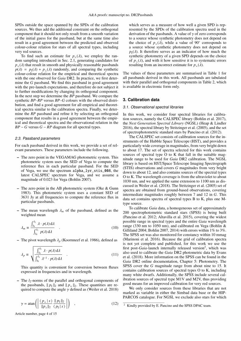
which serves as a measure of how well a given SPD is rep-resented by the SPDs of the calibration spectra used in thederivation of the passbands. A value of γ of zero correspondsto a source whose synthetic photometry does not depend onthe choice of p⊥(λ), while a value of 90◦ corresponds toa source whose synthetic photometry does not depend onp‖(λ). It therefore serves as an indicator of how much thesynthetic photometry of a given SPD depends on the choiceof p⊥(λ), and with it how sensitive it is to systematic errorsresulting from an incorrect estimate for p⊥(λ).

The values of these parameters are summarised in Table 1 forall passbands derived in this work. All passbands are tabulatedwith their parallel and orthogonal components in Table 2, whichis available in electronic form only.

3. Calibration data

3.1. Observational spectral libraries

In this work, we consider four spectral libraries for calibra-tion sources, namely the CALSPEC library (Bohlin et al. 2017),the Next Generation Spectral Library (NGSL) (Heap & Lindler2016), the spectral library by Stritzinger et al. (2005), and the setof spectrophotometric standard stars by Pancino et al. (2012).

The CALSPEC set consists of calibration sources for the in-struments of the Hubble Space Telescope (HST), and provides aparticularly wide coverage in magnitudes, from very bright downto about 17. The set of spectra selected for this work containssources of spectral type O to K that fall in the suitable mag-nitude range to be used for Gaia DR2 calibration. The NGSLlibrary is based on HST/Space Telescope Imaging Spectrograph(STIS) observations and covers G magnitudes from very brightdown to about 12, and also contains sources of the spectral typesO to K. The wavelength coverage is from the ultraviolet to about1030 nm, and we applied the same extension to 1100 nm as dis-cussed in Weiler et al. (2018). The Stritzinger et al. (2005) set ofspectra are obtained from ground-based observations, coveringintermediate magnitudes roughly between 7 and 12 in G. Thisdata set contains spectra of spectral types B to K, plus one M-type source.

To calibrate Gaia data, a homogeneous set of approximately200 spectrophotometric standard stars (SPSS) is being built(Pancino et al. 2012; Altavilla et al. 2015), covering the widestpossible range in spectral types and the entire Gaia wavelengthrange (330 nm to 1050 nm), and calibrated on Vega (Bohlin &Gilliland 2004; Bohlin 2007, 2014) with errors within 1% to 3%.The SPSS set was also monitored for constancy within 10 mmag(Marinoni et al. 2016). Because the grid of calibration spectrais not yet complete and published, for this work we use thefirst post-Gaia-launch internally released version2, which wasalso used to calibrate the Gaia DR2 photometric data by Evanset al. (2018). More information on the SPSS can be found in theGaia DR2 online documentation, Chapter 5: Photometry. TheSPSS cover the G magnitude range from about nine to 15. Itcontains calibration sources of spectral types O to K, includingmany white dwarfs. Additionally, the SPSS include several cal-ibration sources of spectral type M1V and M2V, thus providinggood means for an improved calibration for very red sources.

We only consider sources from these libraries that are notmarked as variable in either the Simbad data base or the HIP-PARCOS catalogue. For NGSL we exclude also stars for which

2 Kindly provided by E. Pancino and the SPSS DPAC team.



Fig. 1. Mean functions and first four functional principal components for the four different spectral libraries. All functions are plotted in the samescale and the eigenfunctions are normalised with respect to the l2-norm. The numbers give the associated eigenvalues and the cumulative fractionof variance explained (FVE).

no slit throughput correction could be applied. For the compar-ison with Gaia DR2 photometry we introduce a lower limit inmagnitude. As reported by Evans et al. (2018), bright sourcesare affected by saturation effects. To exclude such effects fromaffecting the determination of the passbands, we restrict our cal-ibration sources to G magnitudes larger than 5.9. For brighterobjects strong systematic effects in G residuals due to saturationare detectible. For BP and RP, the dispersion of Gaia observa-tions allows for the observation of brighter objects without no-table saturation effects, and we chose a lower magnitude limitof 5.0. A slightly lower limit may still be possible, but to ruleout saturation effects even for sources with extreme colours, wechose the conservative limit of 5.0.

The selected stars were crossmatched with the Gaia DR2,resulting in a set of 45 CALSPEC sources, 210 NGSL sources,72 Stritzinger sources, and 92 SPSS. Functional principal com-ponent analysis was then applied to each of these four sets ofspectra independently to construct four sets of basis functions{ϕ j(λ)} j, analogous to Weiler et al. (2018). The mean functionand the first four functional principal components are shownin Fig. 1 for the four data sets for illustration. The principalcomponents are normalised with respect to the l2-norm, andthe corresponding eigenvalues, displayed in Fig. 1, describe theweight each component has in describing the entire data set. Fig-ure 1 also includes the cumulative fraction of variance explained(FVE), indicating the rather low dimensionality of the data set.With a linear combination of four principal components, a 99%-

level in the capture of the variance of the spectral data sets isachieved.

The principal components show typical features of stellarspectra. However, they do not have any physical meaning inthemselves, but rather provide a compact empirical descriptionof the set of stellar spectra used to generate them. They thusdepend on the underlying set of stellar spectra, which is differ-ent for the different spectral libraries, resulting in different func-tions. There are also features visible in the principal componentsthat are most likely not of astrophysical origin, such as abrupt”jumps” with wavelength in some of the principal components.Prominent features of this kind can be seen in the fourth princi-pal component of the CALSPEC set, which shows a clear dis-placement between about 801.5 nm and 1015.5 nm, and a lessprominent one at 565 nm in the second principal componentof the NGSL set. These discontinuities result from combiningspectra on different wavelength intervals into a single one. Inthe CALSPEC set, the discontinuity at 801.5 nm results froma single spectrum, for which the combination of spectral dataon two wavelength intervals results in a strong abrupt change inthe noise level. This change results in an artefact in the fourthprincipal component. The broader feature at around 1015 nm inthe CALSPEC data set is also an artefact from the combinationof different data to a single spectrum, but the combination oc-curs for many spectra and at slightly different wavelengths. Asa consequence this artefact in the functional principal compo-nents is less localised in wavelength. The discontinuity in thesecond principal component for the NGSL data set is caused by



a small discontinuity when combining spectra obtained with twodifferent gratings to a single one. This effect is in fact very smallin any individual spectrum, but it occurs systematically and istherefore already included in the second principal component.Although the discontinuities in the principal components havelittle impact on the SPD of any particular source, as the projec-tion of the SPD onto these principal components is small, theprojection of the passband onto these principal components maynot be small. The artefacts may therefore become amplified andresult in unphysical parallel components p‖(λ). These featuresdo not pose difficulties in the estimation of the passband p(λ), astheir effect can easily be compensated for by a suitable choiceof the orthogonal component p⊥(λ). The separation into paralleland orthogonal component, however, may become flawed. Wetherefore seek to avoid discontinuities in the passband determi-nation. The SPSS data set is free from such effects, and togetherwith the wide coverage in different spectral types, we considerthe SPSS set of calibration sources the most suitable for the de-termination of the shape of the Gaia passbands. We thereforedo not combine the different spectral libraries, but rather use theSPSS library as the ”default” set of calibration sources in thepassband determination, and validate the results obtained withthis data set by ensuring that the synthetic magnitudes for the re-maining three sets of calibration sources are in good agreementwith the observed magnitudes as well.

3.2. Empirical and theoretical spectral libraries

As a set of empirical spectra representative of different spectraltypes, we use the Pickles (1998) library of stellar spectra. Thislibrary includes SEDs for all spectral types from O5 to M10, andfor luminosity classes I to V, which were derived from observa-tional spectra. Different metallicities are also included for certainspectral types. Pickles (1998) presents two sets of SEDs, cover-ing the spectral ranges from 115 nm to 1062 nm (the UVILIBlibrary) and from 115 nm to 2.5 µm (the UVKLIB library). Inthis work, we use both.

As a second set of spectra, we make use of the BaSeL 3.1WLBC99 library of stellar spectra (Westera et al. 2002). Thislibrary provides theoretical spectra on a wide grid of effectivetemperatures, surface gravities, and metallicities. We refer to thecolour-colour relations of both the empirical library by Pickles(1998) and the theoretical BaSeL library as the synthetic colour-colour relations. For the optimisation of the passbands, we onlyuse the Pickles (1998) spectra in order to avoid an optimisationof the passbands with respect to any particular astrophysical pa-rameters in the BaSeL library. The BaSeL spectra are rather con-sidered as a test case for the result obtained with the Picklesspectra.

3.3. Gaia DR2 data

In order to compare synthetic colour-colour relationships withobservational ones, we select a set of Gaia DR2 photometric ob-servations. Several issues in the Gaia DR2 photometry that couldaffect the passband determination have been reported by Evanset al. (2018) and Arenou et al. (2018). When selecting Gaia DR2observations for our passband determinations, we avoid these is-sues by applying filters in sky region and in magnitude. To re-duce effects caused by crowding, we exclude the region aroundthe galactic plane within ± 30◦ galactic latitude. To minimiseeffects introduced by inaccurate background correction in theGaia DR2 calibration, we restrict the data set to relatively bright

sources, with BP and RP magnitudes less than 17. To excludethe effects of saturation, as mentioned in Sect. 3.1, we further-more introduce a lower magnitude limit of six in G and five inBP and RP. Furthermore, we only include sources for which atleast ten photometric observations in each band entered in thecomputation of the Gaia DR2 mean photometry.

Excluding the galactic plane from our Gaia DR2 data set alsoavoids sources whose SPDs are extremely reddened by interstel-lar extinction. In order to estimate the influence of interstellarextinction on the colour-colour relations used in this work, weapplied the extinction law by Cardelli et al. (1989) to the Picklesspectra, and computed the colour-colour relations resulting fordifferent colour excesses E(B − V) in the regions of the colour-colour diagrams studied in this work. The results are shown inFig. 2. For the BP − RP versus BP − G case, stars follow a rel-atively narrow path running close to diagonal through the dia-gram. To avoid an inconveniently large figure with many whiteareas, we therefore rotate the diagram by 30◦ for a more con-venient fit of the path within a rectangular plotting region. Themain effect of extinction is a shift along the path of the un-reddened spectra in the colour-colour diagram, with only smalldisplacements away from this path. The conclusions in this workdrawn from comparisons between synthetic and observationalcolour-colour relations will therefore not be influenced by inter-stellar reddening.

4. G passband

4.1. Determination of the passband

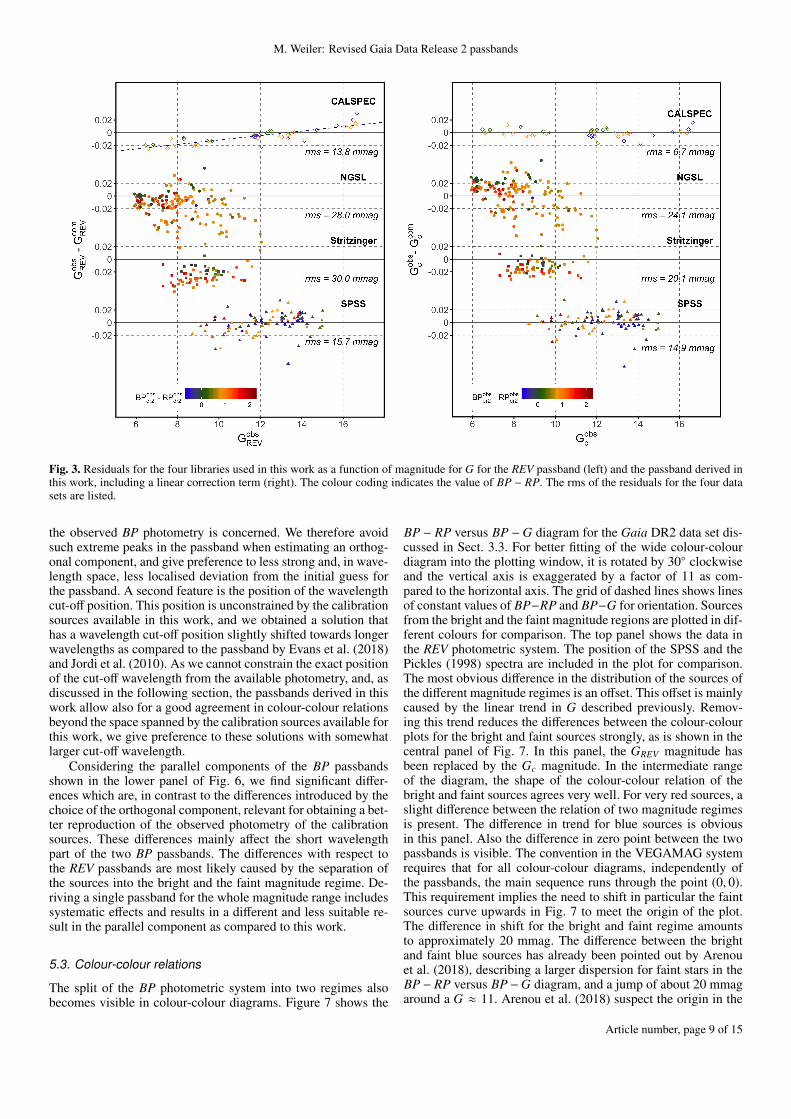
Using the G passbands from Evans et al. (2018), one obtains theresiduals for the four spectral libraries shown in Fig. 3, left panel,plotted versus magnitude. The BP − RP colour of the sources isindicated by the colour coding. This plot differs from the corre-sponding plot in Evans et al. (2018) only because of the differentcriteria in the selection of sources that enter into the plot, andit is repeated here for easy direct comparison. The root meansquare (rms) values of the residuals for the four different sets ofspectra are included in the figure. The dominant feature in theresiduals is a magnitude dependency, which is most clearly vis-ible for the CALSPEC data set, as it has a low random noiseand covers the widest range of magnitudes. A systematic trendin CALSPEC residuals with magnitude has already been men-tioned by Evans et al. (2018), and Arenou et al. (2018) reporteda trend in the G − BP residuals with G magnitude in the orderof a few milli-magnitudes per magnitude. We thus confirm thistrend within a range of G magnitudes between about six and 17.Using the CALSPEC data set, we find it well approximated witha colour-independent linear correction of 3.5 mmag/magnitude,with an uncertainty of about ±0.3 mmag/magnitude. As the cor-rection is on the level of a few tens of a milli-magnitude, a linearcorrection in magnitude and a linear correction in flux is virtu-ally equivalent, and we choose a correction in magnitude for itsmore convenient formulation in magnitude systems. An approx-imately linear drift in the G photometric system with magnitudewas already reported for the Gaia Data Release 1 (Weiler et al.2018) and the reason for this remains unclear for the time being.

The drift in the G magnitude may affect the determination ofthe passband, even if independent from the colour, as the cali-bration sources have a non-uniform distribution of colours withapparent magnitude, the red sources being in tendency brighterthan the blue sources. We therefore correct the G photometry byintroducing a linear correction term in magnitude before deter-



Fig. 2. Position of stellar spectra by Pickles (1998) incolour-colour diagrams for different levels of interstellarreddening. Top panel: The region of the BP − RP versusBP − G diagram considered in Sect. 5. The colour-colourdiagram is rotated clockwise by 30◦ and exaggerated inthe vertical direction by a factor 11. The dashed lines cor-respond to constant BP−RP and BP−G values. Left panel:The red-end region of the BP −G versus G − RP diagramused in Sect. 6.

mining the G passband, that is, we assume a relationship of

Gc = 0.9965 · (−2.5) · log10 (IG) + zp (13)

between IG, the observed counts in the G passband (in electronsper second within the Gaia aperture), and the Gc magnitude. Thefactor of 0.9965 compensates for a linear tendency in magni-tude corresponding to a fading of 3.5 mmag per magnitude andzp denotes the zero-point of the passband, derived as describedin Sect. 2.3. For synthetic photometry in the G band, the fac-tor 0.9965 is not required, as only the observational magnitudeshave to be corrected for the observed trend.

For the determination of p‖(λ) we use the SPSS data set withM = 5 basis functions. We solve Eq. (3) to obtain p‖(λ), andthen estimate the full passband p(λ) as outlined in Sect. 2.1. Asthe initial guess, pini(λ), we use the G passband by Jordi et al.(2010). The residuals obtained with the passband solution de-rived in this work are shown in Fig. 3, right panel, together withthe rms values of the residuals. The passband solution of thiswork is shown in Fig. 4, with the sum of the parallel and orthog-onal component in the upper panel and the parallel component in

the lower panel. Table 1 includes the passband parameters suchas the zero points in the VEGAMAG and AB system, the meanand pivot wavelength, and the l2-norms of the parallel and or-thogonal component. The G passband derived in this work istabulated in Table 2, separated into its parallel and orthogonalcomponents.

4.2. Comparison with other results

The passband obtained in this work is similar to the one derivedby Evans et al. (2018) and presented by Jordi et al. (2010), whichis also presented in Fig. 4 for comparison. The solution of thiswork is slightly steeper at long wavelengths and flatter at in-termediate wavelengths. Comparing the parallel component, theresult of this work is again similar to the G passbands by Evanset al. (2018) and Jordi et al. (2010). Given the uncertainties esti-mated from the residuals, all three G passband solutions are es-sentially equivalent. We thus find the G passband in close agree-ment with the pre-launch expectation and the solution presented



by Evans et al. (2018). This is in contrast to the results for theGaia Data Release 1, where significant deviations from the pre-launch expectation were reported by Maíz Apellániz (2017) andWeiler et al. (2018). The deviations from the pre-launch expecta-tion was explained by the effect of contamination of optical sur-faces in the Gaia instruments present in the early stages of datacollection. The current result may therefore be an indicator of re-duced contamination and of an improvement in the instrumentalcalibration. The major effect for the G passband achieved in thiswork results from the linear correction of the tendency observedin G magnitudes. The correction results in a reduction of the rmsof the residuals for all four sets of spectra considered. As theimprovement is achieved by correcting a systematic effect, thechange in rms, however, depends on the sources considered, andthe quantitative improvement cannot be generalised.

5. BP passband


The residuals for the BP passband resulting from the use of theREV passband by Evans et al. (2018) are shown in the left panelof Fig. 5. The residuals are plotted versus BP – RP colour andgrouped into two sets by Gdr2 magnitude. Sources fainter than10.99 mag and brighter than 10.99 mag are plotted in differentcolours. A colour-dependent systematic behaviour in the resid-uals can be spotted, with blue sources brighter than 10.99 magin G band systematically rising upwards, while the residuals forthe fainter sources slightly decreasing with decreasing BP – RPcolour index. This separation, visible from a BP – RP colour ofabout zero downwards, is consistent with all four sets of calibra-tion sources used in this work. For the CALSPEC data set, allsources in the colour range of BP – RP less than zero belong tothe faint group, and their residuals all belong to the lower group.For the NGSL and Stritzinger sets, all sources in the blue partbelong to the bright group, and all their residuals show the in-creasing tendency with decreasing colour index. For the SPSS,most sources in the blue range belong to the faint G magni-tude range, and the corresponding residuals fall within the lowergroup. Three of the SPSS with BP – RP, however, belong to thebright group with Gdr2 < 10.99, and their residuals also followthe increasing trend. The precise location of the magnitude breakcannot be determined within this work. For the calibration spec-tra available, the optimal separation occurs within the range of10.47 and 10.99 in Gdr2. Depending on whether we admit an”outlier” from the bright or faint magnitude regime, even largeror smaller values are possible. Here, we adopt the value of Gdr2= 10.99 as an estimate for the point of separation between thetwo regimes.

The observed behaviour can be explained by the sourcesfainter than 10.99 in Gdr2 not being in the same photometric sys-tem as the brighter sources. This inconsistency mostly affectsvery blue sources with a BP – RP colour index less than zero.Such an inconsistency may result from sources observed underspecific instrumental configurations failing to converge to a com-mon photometric system during the calibration process, sincebright sources are rarer than faint sources while the complex-ity of the instrument that needs to be taken into considerationin the calibration process is the same for sources of all magni-tudes. Extremely blue sources are also rare. As a consequence,it might be difficult to precisely link the photometric system ofbright blue sources with the photometric system of faint sourcesif they are observed in different instrumental configurations. Apossible change in instrumental configuration for sources in the

observed magnitude range may be a change in CCD gate ac-tivation, a mechanism that is used by the Gaia instruments toadjust the effective exposure time for brighter sources (Carrascoet al. 2016). Another change in instrument configuration is thetransition between two Gaia window classes, resulting in one-dimensional and two-dimensional spectra, respectively. Thesespectra are the basis for deriving the BP and RP magnitudes, andthe change in window class is expected around G ≈ 11.5 (Car-rasco et al. 2016). The exact reason for the discrepancy betweenblue sources in the two different magnitude regimes, however,remains unknown. Changes in the instrumental configuration,however, are driven by the on-board estimate of the G magni-tude, which is the reason why we specify the location of incon-sistency in the BP photometric system by the G magnitude.

To account for this feature in BP magnitude, we separate therange of G magnitudes into two regimes, the ”bright” range forsources with Gdr2 < 10.99 and the ”faint” range for sources withGdr2 > 10.99. We then derive the BP passband separately in thetwo magnitude ranges. We want to use only one set of calibrationsources in both magnitude regimes in order to ensure a consis-tent solution between both. Only the SPSS and the CALSPEClibraries cover both regimes, and for the bright regime the num-ber of sources is rather small. The CALSPEC data set providesa lower random noise for the bright spectra than the SPSS, andwe prefer to use the CALSPEC spectra in this particular case.This set provides similar numbers of sources in the ”bright”and ”faint” regime, although with different coverage in spectraltypes. To compensate for this effect, we adjust the estimate forthe orthogonal components of the two BP passbands such that agood result is achieved for the sources in the other three sets ofspectra as well.

For both the bright and the faint regime in BP we use M = 4basis functions when computing the parallel component, and usecubic B-splines for the modification of the nominal pre-launchBP passband. The residuals obtained with the resulting pass-bands are also shown in Fig. 5, right panel. A significant im-provement can be achieved with the two passbands. The rmsvalues of the residuals, included in Fig. 5, improve for all foursets of spectra. Again, however, as the modifications introducedfor the BP passband correct for systematic effects in the calibra-tion, the resulting differences depend on the particular sourcesconsidered, and the quantitative improvement cannot be gener-alised. The passbands for the bright and faint magnitude regimesare shown in Fig. 6, together with the BPREV passband by Evanset al. (2018) and the BP passband by Jordi et al. (2010) for com-parison. The basic parameters and zero points for the two BPpassbands are listed in Table 1, the parallel and orthogonal com-ponents for both the bright and faint BP passband are tabulatedin Table 2.

The orthogonal components of the BP passbands for thebright and faint regime were chosen in this work in such a waythat the resulting passbands are similar to each other. Apart fromthe difference in shape, we find a difference of about 20 mmag inthe zero points of the passbands for the two magnitude regimes.


Comparing the BP passbands derived in this work with pre-viously published results, strong differences can be observed.Some of these differences occur only in the orthogonal com-ponent of the passband. Among these is the strong peak in theresponse of the BPREV passband around 350 nm. Such a strong,rather localised deviation between the initial expectation and theoptimised passband is not required as far as the reproduction of



Fig. 3. Residuals for the four libraries used in this work as a function of magnitude for G for the REV passband (left) and the passband derived inthis work, including a linear correction term (right). The colour coding indicates the value of BP − RP. The rms of the residuals for the four datasets are listed.

the observed BP photometry is concerned. We therefore avoidsuch extreme peaks in the passband when estimating an orthog-onal component, and give preference to less strong and, in wave-length space, less localised deviation from the initial guess forthe passband. A second feature is the position of the wavelengthcut-off position. This position is unconstrained by the calibrationsources available in this work, and we obtained a solution thathas a wavelength cut-off position slightly shifted towards longerwavelengths as compared to the passband by Evans et al. (2018)and Jordi et al. (2010). As we cannot constrain the exact positionof the cut-off wavelength from the available photometry, and, asdiscussed in the following section, the passbands derived in thiswork allow also for a good agreement in colour-colour relationsbeyond the space spanned by the calibration sources available forthis work, we give preference to these solutions with somewhatlarger cut-off wavelength.

Considering the parallel components of the BP passbandsshown in the lower panel of Fig. 6, we find significant differ-ences which are, in contrast to the differences introduced by thechoice of the orthogonal component, relevant for obtaining a bet-ter reproduction of the observed photometry of the calibrationsources. These differences mainly affect the short wavelengthpart of the two BP passbands. The differences with respect tothe REV passbands are most likely caused by the separation ofthe sources into the bright and the faint magnitude regime. De-riving a single passband for the whole magnitude range includessystematic effects and results in a different and less suitable re-sult in the parallel component as compared to this work.


The split of the BP photometric system into two regimes alsobecomes visible in colour-colour diagrams. Figure 7 shows the

BP − RP versus BP −G diagram for the Gaia DR2 data set dis-cussed in Sect. 3.3. For better fitting of the wide colour-colourdiagram into the plotting window, it is rotated by 30◦ clockwiseand the vertical axis is exaggerated by a factor of 11 as com-pared to the horizontal axis. The grid of dashed lines shows linesof constant values of BP−RP and BP−G for orientation. Sourcesfrom the bright and the faint magnitude regions are plotted in dif-ferent colours for comparison. The top panel shows the data inthe REV photometric system. The position of the SPSS and thePickles (1998) spectra are included in the plot for comparison.The most obvious difference in the distribution of the sources ofthe different magnitude regimes is an offset. This offset is mainlycaused by the linear trend in G described previously. Remov-ing this trend reduces the differences between the colour-colourplots for the bright and faint sources strongly, as is shown in thecentral panel of Fig. 7. In this panel, the GREV magnitude hasbeen replaced by the Gc magnitude. In the intermediate rangeof the diagram, the shape of the colour-colour relation of thebright and faint sources agrees very well. For very red sources, aslight difference between the relation of two magnitude regimesis present. The difference in trend for blue sources is obviousin this panel. Also the difference in zero point between the twopassbands is visible. The convention in the VEGAMAG systemrequires that for all colour-colour diagrams, independently ofthe passbands, the main sequence runs through the point (0, 0).This requirement implies the need to shift in particular the faintsources curve upwards in Fig. 7 to meet the origin of the plot.The difference in shift for the bright and faint regime amountsto approximately 20 mmag. The difference between the brightand faint blue sources has already been pointed out by Arenouet al. (2018), describing a larger dispersion for faint stars in theBP − RP versus BP −G diagram, and a jump of about 20 mmagaround a G ≈ 11. Arenou et al. (2018) suspect the origin in the



Fig. 4. The solution for the G passband (upper panel) and the parallelcomponent (lower panel). Blue line: Jordi et al. (2010). Red line: Evanset al. (2018) (REV), black line shaded: This work.

Table 1. Mean wavelength λm, pivot wavelength λp, zero points in theVEGAMAG and AB photometric systems, and l2-norms of parallel andorthogonal components for Gc, BPc (bright), BPc ( f aint), and RPc passbandsderived in this work.

parameter Gc BPc (bright) BPc ( f aint) RPc

λm [nm] 639.74 516.47 511.78 783.05λp [nm] 622.88 509.18 503.85 777.49zp [VEGA] 25.6409 25.3423 25.3620 24.7600zp [AB] 25.7455 25.3603 25.3888 25.1185||p‖||2 12.9612 9.7182 9.7241 11.5191||p⊥||2 2.0591 2.3606 2.1347 2.7351

G photometry but leave the reason for the observed effect unex-plained. The results found in this work are thus in good agree-ment with previous findings. We attribute the larger dispersionfor faint sources mainly to the linear drift in the G photometry,and the jump of 20 mmag around G ≈ 11 to the BP photometry.

The bottom panel of Fig. 7 shows the colour-colour diagramfor the Gc, BPc, and RPc passbands derived in this work. Thisplot includes the correction for the zero points for the two BPpassbands. The distribution of the Pickles and BaSeL spectra inthis diagram depends significantly on the choice of the RP pass-band and is discussed in the following section.

6. RP passband


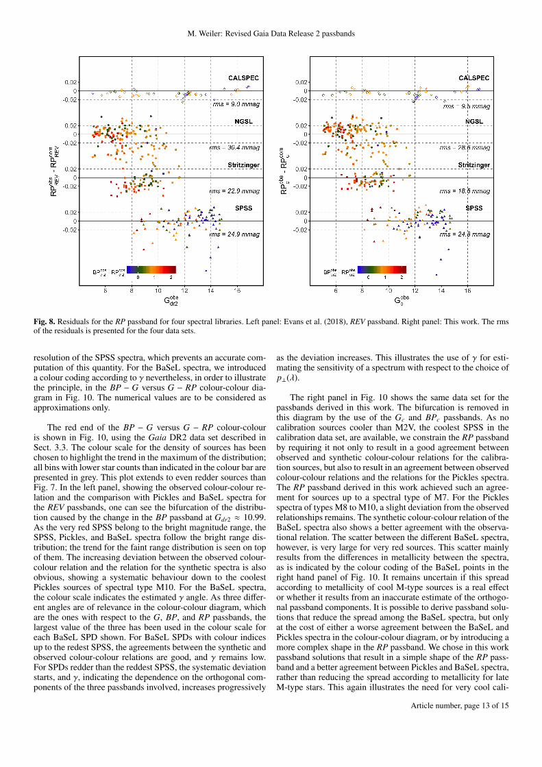
The residuals for the RPREV passband by Evans et al. (2018) areshown on the left panel of Fig. 8. There is a slight tendency to-wards higher residuals for very red sources visible for the SPSSand Stritzinger data sets. The RPdr2 and RPREV passbands werederived with the same set of SPSS calibration sources as used inthis work. The modification of the initial RP passbands by Evanset al. (2018) was done by multiplication with a first degree poly-nomial (see Gaia DR2 online documentation). This choice for amodification model might be too simplistic, not allowing us toproduce a modified passband that has the optimal parallel com-ponent with respect to the calibration sources. As a consequence,a slight colour dependency of the residuals may have remained.

When computing the passband in this work, we cannot con-strain the position of the wavelength cut-on position from pho-tometry alone, as has already been the case for BP discussedbefore. As Evans et al. (2018) had spectroscopic observationsfrom the Gaia RP instrument at hand before deriving the RPpassband from the corresponding integrated photometry, the cut-on position of the passband could be constrained for the RPREVpassband. We therefore chose an orthogonal component of thepassband such that the wavelength cut-on position is the sameas for the Evans et al. (2018) REV passband. We compute theparallel component of the RP passband in this work using theSPSS calibration set with M = 5 basis functions. The orthog-onal component was estimated requiring the passband to repro-duce the observational colour-colour relations, as described inSect. 2.2 and discussed in more detail in Sect. 6.3. The residualsfor the solution of this work are shown in Fig. 8, right panel. Thepassband is shown in Fig. 9. The additional parameters for thepassband are listed in Table 1, and the passband in Table 2. Thepassband solution derived in this work provides an improvementas compared to the REV passband, as it removes the systematiceffect for very red sources in the residuals.


The RP passband derived in this work shows clear differences ascompared to both the solution presented by Evans et al. (2018)and the pre-launch expectation. The differences affect both theparallel and orthogonal components of the passband. The RPpassband derived in this work shows a steeper decrease at longwavelengths as compared to the other RP passbands presentedbefore, and it is flatter at short and intermediate wavelengths.The parallel component derived in this work is lower than forthe REV passband at short wavelengths, and larger at long wave-lengths. The rms values of the residuals, listed in Fig. 8, im-prove slightly for the SPSS, and more strongly for the NGSL andStritzinger spectra. Only for the CALSPEC spectra, the RP pass-band of this work results, for an unknown reason, in a slightlyless good representation than the REV passband.


In Fig. 7 we compare the positions of the Pickles and BaSeLspectra in the BP−RP versus BP−G diagram. For the REV pass-bands, the synthetic follow approximately the observed relationsin the colour-colour diagram, except for the very red sources.For a BP − G colour index larger than approximately 1.25, asystematic deviation between the empirical and synthetic spec-tra and the Gaia DR2 observations occurs. This deviation starts



Fig. 5. Residuals for the BP passband for four spectral libraries. Left panel: Evans et al. (2018), REV passband. Right panel: This work. Residualsfor sources with Gdr2 > 10.99 are plotted in black, sources with Gdr2 < 10.99 in red. The rms of the residuals are listed for the four data sets.

Fig. 6. As Fig. 4, but for BP. Left: Solution for the bright magnitude regime. Right: Solution for the faint magnitude regime.

for sources redder than the reddest SPSS available for calibra-tion. This deviation can be explained by the influence of the or-thogonal component of the passbands. M-type stars show strongvariations in their SPDs, and very cool calibration sources arecurrently not available. As a consequence, the orthogonal com-ponent of the passband becomes increasingly important for thesynthetic photometry of stars as their effective temperature be-

comes lower than the coolest calibration source. And if the guessfor the orthogonal component is not optimal, this dependency onp⊥(λ) manifests itself in a progressive deviation of the syntheticcolour-colour relations for Pickles and BaSeL spectra from theobserved one. This effect may be quantified using the angle γ asdefined in Weiler et al. (2018). For the Pickles and BaSeL spec-tra, however, the wavelength resolution of 500 is lower than the



Fig. 7. Colour-colour diagram for BP − RP versus BP − G, separated into the bright (red shades) and faint (blue shades) magnitude range. Toppanel: REV passbands. The black dots indicate the positions of the Pickles spectra, the green triangles show the SPSS (filled symbols for bright,open symbols for faint range). Central panel: As top panel, but replacing the GREV magnitude by the Gc magnitude of this work. Bottom panel:Same as top panel, but for the Gc, BPc, and RPc magnitudes of this work. The filled dots correspond to the Pickles spectra and the bright range BPpassband, open dots for the BP passband for the faint magnitude range. The orange dots show the BaSeL spectra from the bright range, the cyandots for the faint range. The original colour-colour diagram has been rotated by 30◦ clockwise and exaggerated in a vertical direction by a factorof 11 for better display. The dashed lines indicate the axis grid in BP − RP and BP −G.



Fig. 8. Residuals for the RP passband for four spectral libraries. Left panel: Evans et al. (2018), REV passband. Right panel: This work. The rmsof the residuals is presented for the four data sets.

resolution of the SPSS spectra, which prevents an accurate com-putation of this quantity. For the BaSeL spectra, we introduceda colour coding according to γ nevertheless, in order to illustratethe principle, in the BP − G versus G − RP colour-colour dia-gram in Fig. 10. The numerical values are to be considered asapproximations only.

The red end of the BP − G versus G − RP colour-colouris shown in Fig. 10, using the Gaia DR2 data set described inSect. 3.3. The colour scale for the density of sources has beenchosen to highlight the trend in the maximum of the distribution;all bins with lower star counts than indicated in the colour bar arepresented in grey. This plot extends to even redder sources thanFig. 7. In the left panel, showing the observed colour-colour re-lation and the comparison with Pickles and BaSeL spectra forthe REV passbands, one can see the bifurcation of the distribu-tion caused by the change in the BP passband at Gdr2 ≈ 10.99.As the very red SPSS belong to the bright magnitude range, theSPSS, Pickles, and BaSeL spectra follow the bright range dis-tribution; the trend for the faint range distribution is seen on topof them. The increasing deviation between the observed colour-colour relation and the relation for the synthetic spectra is alsoobvious, showing a systematic behaviour down to the coolestPickles sources of spectral type M10. For the BaSeL spectra,the colour scale indicates the estimated γ angle. As three differ-ent angles are of relevance in the colour-colour diagram, whichare the ones with respect to the G, BP, and RP passbands, thelargest value of the three has been used in the colour scale foreach BaSeL SPD shown. For BaSeL SPDs with colour indicesup to the redest SPSS, the agreements between the synthetic andobserved colour-colour relations are good, and γ remains low.For SPDs redder than the reddest SPSS, the systematic deviationstarts, and γ, indicating the dependence on the orthogonal com-ponents of the three passbands involved, increases progressively

as the deviation increases. This illustrates the use of γ for esti-mating the sensitivity of a spectrum with respect to the choice ofp⊥(λ).

The right panel in Fig. 10 shows the same data set for thepassbands derived in this work. The bifurcation is removed inthis diagram by the use of the Gc and BPc passbands. As nocalibration sources cooler than M2V, the coolest SPSS in thecalibration data set, are available, we constrain the RP passbandby requiring it not only to result in a good agreement betweenobserved and synthetic colour-colour relations for the calibra-tion sources, but also to result in an agreement between observedcolour-colour relations and the relations for the Pickles spectra.The RP passband derived in this work achieved such an agree-ment for sources up to a spectral type of M7. For the Picklesspectra of types M8 to M10, a slight deviation from the observedrelationships remains. The synthetic colour-colour relation of theBaSeL spectra also shows a better agreement with the observa-tional relation. The scatter between the different BaSeL spectra,however, is very large for very red sources. This scatter mainlyresults from the differences in metallicity between the spectra,as is indicated by the colour coding of the BaSeL points in theright hand panel of Fig. 10. It remains uncertain if this spreadaccording to metallicity of cool M-type sources is a real effector whether it results from an inaccurate estimate of the orthogo-nal passband components. It is possible to derive passband solu-tions that reduce the spread among the BaSeL spectra, but onlyat the cost of either a worse agreement between the BaSeL andPickles spectra in the colour-colour diagram, or by introducing amore complex shape in the RP passband. We chose in this workpassband solutions that result in a simple shape of the RP pass-band and a better agreement between Pickles and BaSeL spectra,rather than reducing the spread according to metallicity for lateM-type stars. This again illustrates the need for very cool cali-



Fig. 9. As Fig. 4, but for RP.

bration sources in order to allow for a reliable interpretation ofthe photometry of M-type stars.

7. Summary and conclusions

In this work, we determined the G, BP, and RP passbands forGaia DR2. We used a functional analytic formulation of theproblem of passband reconstruction to separate each passbandinto a sum of two functions. One of these functions, the parallelcomponent p‖(λ), is fully constrained by the calibration sources,while the other function, the orthogonal component p⊥(λ), isfully unconstrained. We derived the parallel component usingsets of observational spectral libraries and the Gaia DR2 pho-tometry of the sources included in the libraries. The orthogonalcomponent is estimated based on two considerations. First, weuse an initial guess for the passband, based on a-priori knowl-edge on the passband shape. This initial guess is then modifiedin such a way that the modified initial guess remains close tothe initial guess while having p‖(λ) in agreement with the de-termination. Second, we introduce an additional constraint onthe choice of the orthogonal component by requiring the pass-bands to predict colour-colour relationships for model spectra ofa wide range of spectral types to be in agreement with the ob-served colour-colour distributions in Gaia DR2.

For the G passband, we found a solution for the shape of thepassband that is basically in agreement with the shape of solu-tions published by Evans et al. (2018) and Jordi et al. (2010).An approximately linear trend in the G photometry is howeverpresent on a magnitude interval from about 6 to 17. A trend inG photometry has already been observed in Gaia Data Release 1

(Weiler et al. 2018), and it was already noticed for Gaia DR2 byEvans et al. (2018) and Arenou et al. (2018). The origin of thiseffect remains yet unknown. In this work, we introduce a cor-rection for it by applying a linear correction in G magnitude of3.5 mmag per magnitude. This correction results in a factor of0.9965 in the computation of the Gc magnitude according to Eq.(13). This correction applies to a magnitude interval from about6 to 17 in G band. For brighter sources, a deviation from thistrend caused by saturation effects occurs, as reported by Evanset al. (2018). For magnitudes larger than 17, no suitable calibra-tion sources are available for this work. Arenou et al. (2018),however, found indications for a more complex systematics inthe residuals for sources fainter than about 17.

For BP we introduced two different photometric systems forstars brighter and fainter than 10.99 in the Gdr2-band. By doingso, we take into account an inconsistency in the BP photome-try, which occurs for a reason as yet unknown, but it may beconnected to a change in instrumental configuration such as gateactivation or windowing. The assumption of two BP passbandsexplains the differences between the G and BP photometry previ-ously reported by Arenou et al. (2018). We derive two passbandsfor BP, valid for sources brighter than 10.99 mag in Gdr2, andfainter than this limit. The BP passbands derived for the brightand the faint magnitude range are rather similar to each otherin shape, and differ in zero point by about 20 mmag from eachother. However, they differ significantly from previously pub-lished passbands by Evans et al. (2018) and Jordi et al. (2010).

The passband for RP provides an improvement as comparedto the passband by Evans et al. (2018), as it removes a systematiccolour-dependent effect in reproducing the calibration sources.The passband is rather different in shape from the previouslypublished RP passbands.

The passband solutions for G, BP, and RP in this work havebeen chosen such that, when applying them together, the syn-thetic photometry from the Pickles (1998) spectral library isin good agreement with the colour-colour relations observed inGaia DR2. The passbands presented in this work result in syn-thetic colour-colour relations that follow well the observed rela-tions for stars from spectral type O5 to M7. For cooler sourcesthan M7, the database becomes too sparse and the variationwithin synthetic colour-colour relations too large to draw def-inite conclusions. The different passbands derived in this workare thus consistent with each other within the limits set by theavailable calibration data.

We point out that the shapes of the passbands derived in thiswork are not unique, as is the case for the passbands derivedby Evans et al. (2018). The limitation is introduced by the exis-tence of the orthogonal component and is of a fundamental na-ture. There necessarily exist an infinite number of different pass-bands that describe all available calibration data equally well. Inorder to estimate the sensitivity of a particular SPD with respectto the orthogonal component, we suggest the computation of thecontribution of p‖(λ) and p⊥(λ) to the synthetic photometry in-dependently. For this purpose, all passbands derived in this workare presented in Table 2 with their parallel and orthogonal com-ponents individually. The angle γ as defined in Eq. 12 may serveas an illustrative quantity for specifying the degree to which aparticular SPD depends on the orthogonal component and, withit, how sensitive the synthetic photometry of the given SPD is tosystematic errors that may arise from an inaccurate estimate ofp⊥(λ).

The passbands presented in this work allow for a betteragreement between synthetic and observed photometry over awide range of SPDs than previously published passbands, while



Fig. 10. Left panel: Colour-colour diagram for the REV passbands. The black circles indicate the positions of the Pickles spectra, the dark greentriangles show the SPSS. The dots represent the BaSeL spectra, colour-coded according to the estimated γ angle. Right panel: Same as left panel,but for the Gc, BPc, and RPc magnitudes of this work. The BaSeL spectra are shown for the faint magnitude range only, and are colour-codedaccording to the metallicity (in dex). Bins with numbers of stars lower than indicated in the colour bars are plotted in grey.

at the same time being physically reasonable. Table 2 lists allpassbands derived in this work as a function of wavelength andis available in electronic form at the Centre de Données as-tronomiques de Strasbourg, CDS. Applying them in the inter-pretation of the Gaia DR2 photometric data may therefore helpto maximise the scientific outcome from the uniquely large andaccurate astronomical data set that is Gaia DR2.Acknowledgements. This work was supported by the MINECO (Spanish Min-istry of Economy) through grants ESP2016-80079-C2-1-R (MINECO/FEDER,UE) and ESP2014-55996-C2-1-R (MINECO/FEDER, UE) and MDM-2014-0369 of ICCUB (Unidad de Excelencia ”María de Maeztu”).This work has made use of data from the European Space Agency (ESA)mission Gaia (https://www.cosmos.esa.int/gaia), processed by the GaiaData Processing and Analysis Consortium (DPAC, https://www.cosmos.esa.int/web/gaia/dpac/consortium). Funding for the DPAC has been pro-vided by national institutions, in particular the institutions participating in theGaia Multilateral Agreement.I thank the Gaia DPAC SPSS team for providing the intermediate data productsused for this work: E. Pancino, G. Altavilla, S. Marinoni, N. Sanna, G. Cocozza,S. Ragaini, and S. Galleti.I furthermore thank C. Jordi, J. M. Carrasco and C. Fabricius for fruitful discus-sions during the preparation of this work.

ReferencesAltavilla, G., Marinoni, S., Pancino, E., et al. 2015, Astronomische Nachrichten,

336, 515Arenou, F., Luri, X., Babusiaux, C., et al. 2018, ArXiv e-prints

[arXiv:1804.09375]Bohlin, R. C. 2007, in Astronomical Society of the Pacific Conference Series,

Vol. 364, The Future of Photometric, Spectrophotometric and PolarimetricStandardization, ed. C. Sterken, 315

Bohlin, R. C. 2014, AJ, 147, 127Bohlin, R. C. & Gilliland, R. L. 2004, AJ, 127, 3508

Bohlin, R. C., Mészáros, S., Fleming, S. W., et al. 2017, AJ, 153, 234Cardelli, J. A., Clayton, G. C., & Mathis, J. S. 1989, ApJ, 345, 245Carrasco, J. M., Evans, D. W., Montegriffo, P., et al. 2016, A&A, 595, A7Evans, D. W., Riello, M., De Angeli, F., et al. 2018, ArXiv e-prints

[arXiv:1804.09368]Gaia Collaboration, Brown, A. G. A., Vallenari, A., et al. 2018, ArXiv e-prints

[arXiv:1804.09365]Gaia Collaboration Prusti, T., de Bruijne, J. H. J., Brown, A. G. A., et al. 2016,

A&A, 595, A1Heap, S. R. & Lindler, D. 2016, in Calibration and Standardization of Missions

and Large Surveys in Astronomy and Astrophysics, ed. S. Deustua, A. Allam,D. Tucker, & J. A. Smith (ASP Conference Series, Vol. 503)

Jordi, C., Gebran, M., Carrasco, J. M., et al. 2010, A&A, 523, A48Koornneef, J., Bohlin, R., Buser, R., Horne, K., & Turnshek, D. 1986, in High-

lights of Astronomy, ed. J.-P. SwingsMaíz Apellániz, J. 2017, A&A, 608, L8Marinoni, S., Pancino, E., Altavilla, G., et al. 2016, MNRAS, 462, 3616Oke, J. B. & Gunn, J. E. 1983, ApJ, 266, 713Pancino, E., Altavilla, G., Marinono, S., et al. 2012, MNRAS, 426, 1767Pickles, A. J. 1998, PASP, 110, 863Stritzinger, M., Suntzeff, N. B., Hamuy, M., et al. 2005, PASP, 117, 810Weiler, M., Jordi, C., Fabricius, C., & Carrasco, J. M. 2018, ArXiv e-prints

[arXiv:1802.01667]Westera, P., Lejeune, T., Buser, R., Cuisinier, F., & Bruzual, G. 2002, A&A, 381,

524


https://www.cosmos.esa.int/gaia

https://www.cosmos.esa.int/web/gaia/dpac/consortium

https://www.cosmos.esa.int/web/gaia/dpac/consortium

Documents

M. Weiler - arxiv.org fileAstronomy & Astrophysics manuscript no. DR2Passbands c ESO 2018 June 27, 2018 Revised Gaia Data Release 2 passbands? M. Weiler Departament de Física Quàntica