1

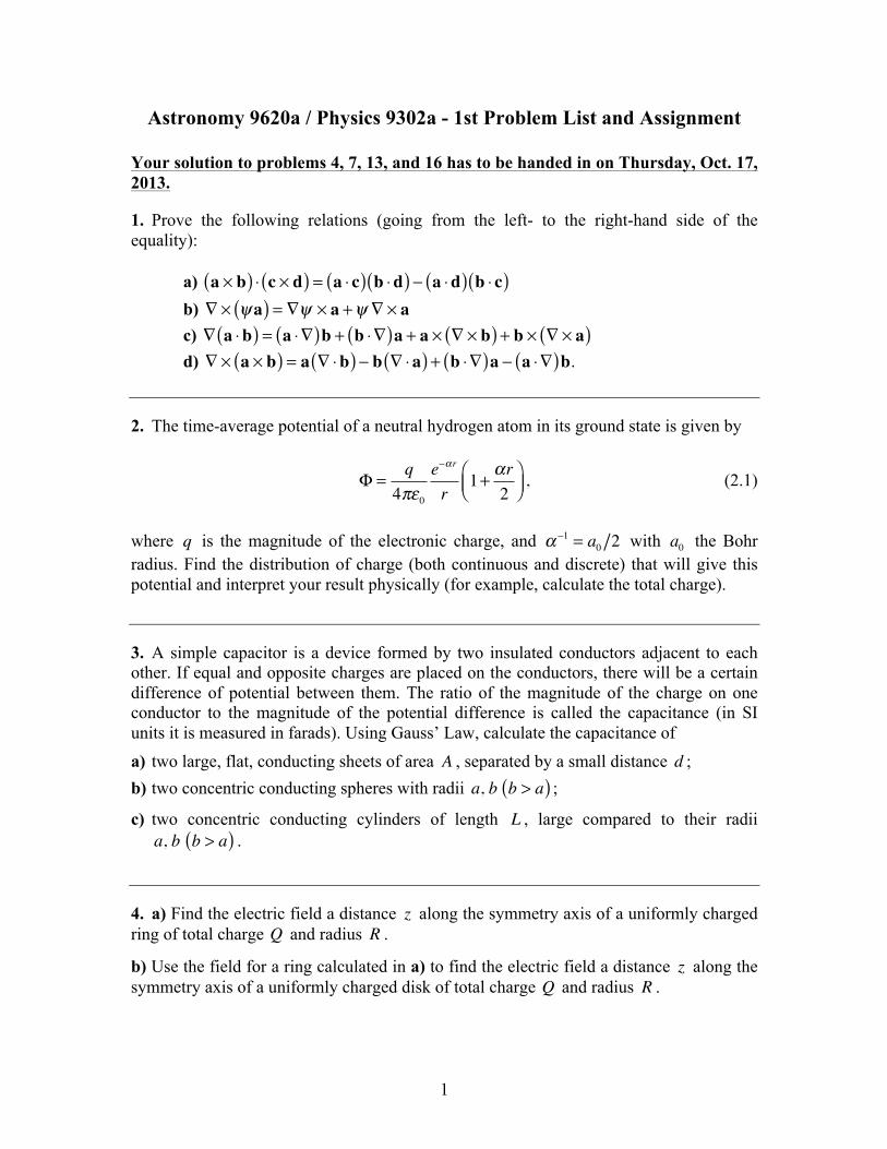
Astronomy 9620a / Physics 9302a - 1st Problem List and Assignment

Your solution to problems 4, 7, 13, and 16 has to be handed in on Thursday, Oct. 17, 2013.

1. Prove the following relations (going from the left- to the right-hand side of the equality):

a) a × b( ) ⋅ c × d( ) = a ⋅ c( ) b ⋅d( ) − a ⋅d( ) b ⋅ c( ) b) ∇ × ψa( ) = ∇ψ × a +ψ ∇ × a c) ∇ a ⋅b( ) = a ⋅∇( )b + b ⋅∇( )a + a × ∇ × b( ) + b × ∇ × a( ) d) ∇ × a × b( ) = a ∇ ⋅b( ) − b ∇ ⋅a( ) + b ⋅∇( )a − a ⋅∇( )b.

2. The time-average potential of a neutral hydrogen atom in its ground state is given by

Φ =q4πε0

e−αr

r1+ αr

2⎛⎝⎜

⎞⎠⎟, (2.1)

where q is the magnitude of the electronic charge, and α−1 = a0 2 with a0 the Bohr radius. Find the distribution of charge (both continuous and discrete) that will give this potential and interpret your result physically (for example, calculate the total charge).

3. A simple capacitor is a device formed by two insulated conductors adjacent to each other. If equal and opposite charges are placed on the conductors, there will be a certain difference of potential between them. The ratio of the magnitude of the charge on one conductor to the magnitude of the potential difference is called the capacitance (in SI units it is measured in farads). Using Gauss’ Law, calculate the capacitance of a) two large, flat, conducting sheets of area A , separated by a small distance d ; b) two concentric conducting spheres with radii a, b b > a( ) ;

c) two concentric conducting cylinders of length L , large compared to their radii a, b b > a( ) .

4. a) Find the electric field a distance z along the symmetry axis of a uniformly charged ring of total charge Q and radius R .

b) Use the field for a ring calculated in a) to find the electric field a distance z along the symmetry axis of a uniformly charged disk of total charge Q and radius R .

2

c) Use the results of b) to find the electric field due to the charged disk at z = 0 and z R . For the latter, would it have been possible to derive this result based simply on physical arguments? Explain your answer.

5. Electrostatic Screening and the Debye Length. Let’s assume that we have a system consisting of distributions (i.e., number densities in m−3 ) ne and ni of electrons and positive ions, respectively. The distributions are initially in equilibrium with homogeneous densities ne = ni (independent of position), such that the electrostatic potential Φ is zero everywhere. We now introduce a charge Q that locally perturbs the distributions of electrons and ions, and destroys their homogeneity in its vicinity. If we assume that far away from the charge both densities still have the same value n , then we can expect from thermodynamic equilibrium considerations that the following relations will hold in the neighborhood of Q

ni = ne

−qΦκBT

ne = neqΦκBT ,

(5.1)

where q, κ B, and T are the charge of the ions (−q for the electrons), the Boltzmann constant, and the temperature of the system, respectively. a) Use equations (5.1) and the Poisson equation to show that the electrostatic potential around Q is given by

Φ r( ) = Q4πε0r

e−rλD , (5.2)

where r is the distance (radius) away from Q and

λD =ε0κ BT2nq2

⎛⎝⎜

⎞⎠⎟

1 2

(5.3)

is the so-called Debye length. To obtain equation (5.2) you can safely assume that qΦ κ BT( ) is a small quantity, such that it is appropriate to linearize the exponentials of equations (5.1). Also, assume that the electrostatic potential is zero at infinity. b) Using just a few sentences, explain the physical implication of equation (5.2). That is, what is the spatial extent over which the presence of Q is felt? Over what length scale can this plasma be considered neutral? [Hints: Poisson’s equation is

3

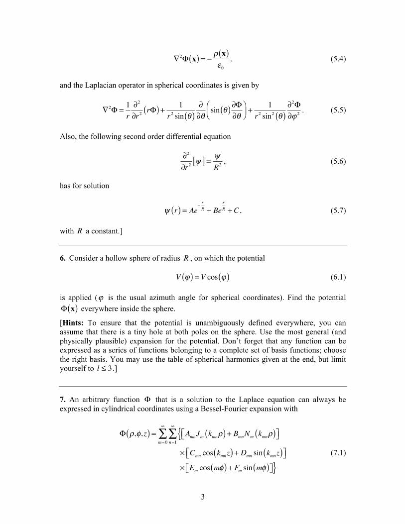
∇2Φ x( ) = −ρ x( )ε0

, (5.4)

and the Laplacian operator in spherical coordinates is given by

∇2Φ =1r∂2

∂r2rΦ( ) + 1

r2 sin θ( )∂∂θ

sin θ( ) ∂Φ∂θ

⎛⎝⎜

⎞⎠⎟+

1r2 sin2 θ( )

∂2Φ∂ϕ 2 . (5.5)

Also, the following second order differential equation

∂2

∂r2ψ[ ] = ψ

R2, (5.6)

has for solution

ψ r( ) = Ae−rR + Be

rR + C, (5.7)

with R a constant.]

6. Consider a hollow sphere of radius R , on which the potential V ϕ( ) = V cos ϕ( ) (6.1) is applied (ϕ is the usual azimuth angle for spherical coordinates). Find the potential Φ x( ) everywhere inside the sphere.

[Hints: To ensure that the potential is unambiguously defined everywhere, you can assume that there is a tiny hole at both poles on the sphere. Use the most general (and physically plausible) expansion for the potential. Don’t forget that any function can be expressed as a series of functions belonging to a complete set of basis functions; choose the right basis. You may use the table of spherical harmonics given at the end, but limit yourself to l ≤ 3 .]

7. An arbitrary function Φ that is a solution to the Laplace equation can always be expressed in cylindrical coordinates using a Bessel-Fourier expansion with

Φ ρ,φ, z( ) = AmnJm kmnρ( ) + BmnNm kmnρ( )⎡⎣ ⎤⎦{n=1

∞

∑m=0

∞

∑× Cmn cos kmnz( ) + Dmn sin kmnz( )⎡⎣ ⎤⎦× Em cos mφ( ) + Fm sin mφ( )⎡⎣ ⎤⎦}

(7.1)

4

where Jm x( ) and Nm x( ) are the Bessel functions of, respectively, the first and second kind of order m , and it is implicit that F0 = 0 and E0 agrees with the usual definition for the corresponding Fourier coefficient (see Equation (2.2) of the Lecture Notes). The functions’ behaviors at the origin are such Jm 0( ) is finite and well behaved whereas Nm 0( ) is not. The validity of equation (7.1) stems, in part, from the fact that the set of Bessel functions is complete and forms a basis, such that any function f ρ( ) can be expanded over a given interval for ρ of length a with

f ρ( ) = αmnJm kmnρa

⎛⎝⎜

⎞⎠⎟+ βmnNm kmn

ρa

⎛⎝⎜

⎞⎠⎟

⎡⎣⎢

⎤⎦⎥n=1

∞

∑m=0

∞

∑ , (7.2)

where

αmn =

2a2Jm+1

2 kmn( ) ρ f ρ( )Jm kmnρa

⎛⎝⎜

⎞⎠⎟dρ∫

βmn =2

a2Nm+12 kmn( ) ρ f ρ( )Nm kmn

ρa

⎛⎝⎜

⎞⎠⎟dρ∫

(7.3)

and the integrals are performed over the aforementioned interval. Now consider a hollow cylindrical tube of radius a , with its axis of symmetry coincident with the z-axis , and its ends located at z = 0 and z = L . The potential on its end faces is zero, while the potential on the cylinder is given as

V φ, z( ) = V for − π 2 < φ < π 2−V for π 2 < φ < 3π 2.

⎧⎨⎪

⎩⎪ (7.4)

Find the potential anywhere inside the cylinder.

8. Prove the following theorem: For an arbitrary charge distribution ρ x( ) the values of the 2l +1( ) moments of the first non-vanishing multipole are independent of the origin of the coordinate axes, but the value of all higher multipole moments do in general depend on the choice of origin. (The different moments qlm for fixed l depend, of course, on the orientation of the axes.)

5

9. Given that the potential Φ x( ) due to a charge distribution ρ ′x( ) can be evaluated with the following relation

Φ x( ) = 14πε0

ρ ′x( )x − ′x

d 3 ′x∫ , (9.1)

expand 1 x − ′x with a Taylor series (see equation (1.84) of the lecture notes) to show that

Φ x( ) 1

4πε0

qr+p ⋅xr3

+12Qij

xix jr5

+⎡⎣⎢

⎤⎦⎥, (9.2)

where a summation on a repeated index is assumed, and

q = ρ ′x( )∫ d 3 ′x

p = ′x ρ ′x( )∫ d 3 ′x

Qij = 3 ′xi ′x j − ′r 2δ ij( )ρ ′x( )∫ d 3 ′x .

(9.3)

10. A perfectly conducting object has a hollow cavity in its interior. If a point charge is introduced in the cavity, what is the total charge induced on the surface of the cavity.

11. An electric dipole is pointing in the z direction and is placed at the origin of the coordinate system. Find the value of the electric field at any point.

12. We know that the force F acting on a charge q is given by F = qE , where E is the electric field at the position of the charge.

a) Now, consider a charge distribution ρ x( ) and write down the general expression for the total force acting on it. b) We choose a position x0 as the “origin” for calculating the different multipole moments of the distribution. Show that the force acting on the electric dipole moment is Fd = p ⋅∇( )E, (12.1) where p is the dipole moment, and it is understood that the gradient is evaluated at x0 .

6

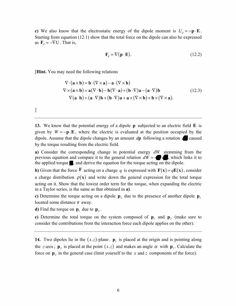
c) We also know that the electrostatic energy of the dipole moment is Ud = −p ⋅E . Starting from equation (12.1) show that the total force on the dipole can also be expressed as Fd = −∇U . That is, Fd = ∇ p ⋅E( ). (12.2) [Hint. You may need the following relations

∇ ⋅ a × b( ) = b ⋅ ∇ × a( ) − a ⋅ ∇ × b( )∇ × a × b( ) = a ∇ ⋅b( ) − b ∇ ⋅a( ) + b ⋅∇( )a − a ⋅∇( )b

∇ a ⋅b( ) = a ⋅∇( )b + b ⋅∇( )a + a × ∇ × b( ) + b × ∇ × a( ). (12.3)

]

13. We know that the potential energy of a dipole p subjected to an electric field E is given by W = −p ⋅E , where the electric is evaluated at the position occupied by the dipole. Assume that the dipole changes by an amount dp following a rotation dθ caused by the torque resulting from the electric field. a) Consider the corresponding change in potential energy dW stemming from the previous equation and compare it to the general relation dW = −τ ⋅dθ , which links it to the applied torque τ , and derive the equation for the torque acting on the dipole. b) Given that the force F acting on a charge q is expressed with F x( ) = qE x( ) , consider a charge distribution ρ x( ) and write down the general expression for the total torque acting on it. Show that the lowest order term for the torque, when expanding the electric in a Taylor series, is the same as that obtained in a). c) Determine the torque acting on a dipole p2 due to the presence of another dipole p1 located some distance r away. d) Find the torque on p1 due to p2 .

e) Determine the total torque on the system composed of p1 and p2 (make sure to consider the contributions from the interaction force each dipole applies on the other).

14. Two dipoles lie in the x, z( )-plane . p1 is placed at the origin and is pointing along the z-axis ; p2 is placed at the point x, z( ) and makes an angle α with p1 . Calculate the force on p2 in the general case (limit yourself to the x and z components of the force).

7

15. Find the B field along the symmetry axis of a circular loop of radius a carrying a current I .

16. A small current loop of radius R lies in the x, y( )-plane . A current J passes through the loop. a) Find the magnetic dipole moment m of the loop. b) Find the asymptotic (i.e., r R ) magnetic induction B from the magnetic potential due to m . c) Write the equation of motion for a particle of mass M and charge q in the asymptotic B field of the loop. Show that the particle stays in the x, y( )-plane if its original velocity is restricted to that plane.

17. Magnetostatic problems can be treated in a way similar to electrostatic ones. Show that for the calculation of the fields, a material of magnetization M x( ) can be replaced by a volume polarization charge density ρM = −∇ ⋅M and a surface polarization charge densityσM = n ⋅M .

18. When making a change from a system of Cartesian coordinates x, y, z( ) to another system α,β,γ( ) we find that the volume integral is expressed as dxdydz = J dαdβdγ∫∫∫∫∫∫ , (18.1) where J is the determinant of the Jacobian matrix that expresses the transformation of infinitesimal changes between the two systems of coordinates. More precisely, we have

8

dxdydz

⎛

⎝

⎜⎜

⎞

⎠

⎟⎟ = J

⎡

⎣

⎢⎢⎢

⎤

⎦

⎥⎥⎥

dαdβdγ

⎛

⎝

⎜⎜

⎞

⎠

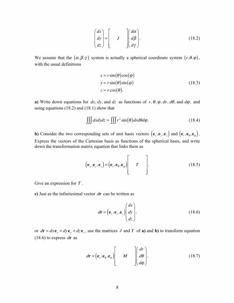
⎟⎟ . (18.2)

We assume that the α,β,γ( ) system is actually a spherical coordinate system r,θ,ϕ( ) , with the usual definitions

x = r sin θ( )cos ϕ( )y = r sin θ( )sin ϕ( )z = r cos θ( ).

(18.3)

a) Write down equations for dx, dy, and dz as functions of r, θ, ϕ, dr, dθ, and dϕ, and using equations (18.2) and (18.1) show that dxdydz = r2 sin θ( )drdθdϕ∫∫∫∫∫∫ . (18.4) b) Consider the two corresponding sets of unit basis vectors ex ,ey ,ez( ) and er ,eθ ,eϕ( ) . Express the vectors of the Cartesian basis as functions of the spherical basis, and write down the transformation matrix equation that links them as

ex ,ey ,ez( ) = er ,eθ ,eϕ( ) T⎡

⎣

⎢⎢⎢

⎤

⎦

⎥⎥⎥. (18.5)

Give an expression for T . c) Just as the infinitesimal vector dr can be written as

dr = ex ,ey ,ez( )dxdydz

⎛

⎝

⎜⎜

⎞

⎠

⎟⎟ , (18.6)

or dr = dx ex + dyey + dzez , use the matrices J and T of a) and b) to transform equation (18.6) to express dr as

dr = er ,eθ ,eϕ( ) M⎡

⎣

⎢⎢⎢

⎤

⎦

⎥⎥⎥

drdθdϕ

⎛

⎝

⎜⎜

⎞

⎠

⎟⎟ , (18.7)

9

or dr = aer + beθ + ceϕ . Give expressions for M , a, b, and c . d) An equivalent way of expressing the infinitesimal Cartesian volume element of equation (18.1) is to use the components of the vector dr = dx ex + dyey + dzez to

calculate dxdydz = dzez ⋅ dx ex × dyey( ) . Similarly, use dr = aer + beθ + ceϕ to verify

that the infinitesimal spherical volume element equals r2 sin θ( )dr dθ dϕ . e) Finally, invert equation (18.5) to obtain

er ,eθ ,eϕ( ) = ex ,ey ,ez( ) T −1

⎡

⎣

⎢⎢⎢

⎤

⎦

⎥⎥⎥, (18.8)

then starting with r = r er verify that dr = aer + beθ + ceϕ .

19. Consider the gradient vector operator ∇ in Cartesian coordinates ∇ = ex∂x + ey∂y + ez∂z , (19.1)

where we used the following short hand notation for the partial derivatives ∂x ≡∂∂x

, etc.

We are interested in investigating the form that this operator takes when we make the change from a Cartesian to a spherical coordinate system. We use the usual definitions

x = r sin θ( )cos ϕ( )y = r sin θ( )sin ϕ( )z = r cos θ( ),

(19.2)

or, alternatively,

r = x2 + y2 + z2

tan θ( ) = x2 + y2

z

tan ϕ( ) = yx.

(19.3)

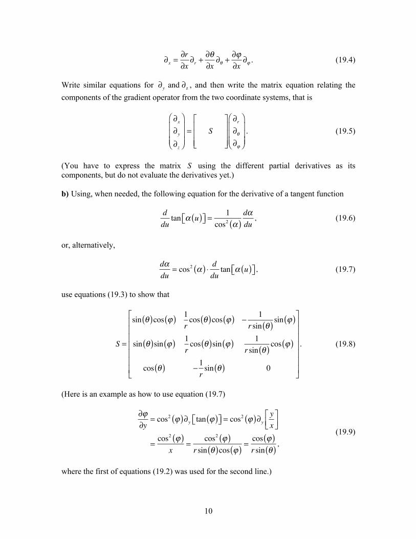
a) Using the chain rule we can write

10

∂x =∂r∂x

∂r +∂θ∂x

∂θ +∂ϕ∂x

∂ϕ . (19.4)

Write similar equations for ∂y and ∂z , and then write the matrix equation relating the components of the gradient operator from the two coordinate systems, that is

∂x∂y∂z

⎛

⎝

⎜⎜⎜

⎞

⎠

⎟⎟⎟= S⎡

⎣

⎢⎢⎢

⎤

⎦

⎥⎥⎥

∂r∂θ∂ϕ

⎛

⎝

⎜⎜⎜

⎞

⎠

⎟⎟⎟. (19.5)

(You have to express the matrix S using the different partial derivatives as its components, but do not evaluate the derivatives yet.) b) Using, when needed, the following equation for the derivative of a tangent function

ddutan α u( )⎡⎣ ⎤⎦ =

1cos2 α( )

dαdu, (19.6)

or, alternatively,

dαdu

= cos2 α( ) ⋅ ddutan α u( )⎡⎣ ⎤⎦, (19.7)

use equations (19.3) to show that

S =

sin θ( )cos ϕ( ) 1rcos θ( )cos ϕ( ) −

1r sin θ( ) sin ϕ( )

sin θ( )sin ϕ( ) 1rcos θ( )sin ϕ( ) 1

r sin θ( ) cos ϕ( )

cos θ( ) −1rsin θ( ) 0

⎡

⎣

⎢⎢⎢⎢⎢⎢⎢

⎤

⎦

⎥⎥⎥⎥⎥⎥⎥

. (19.8)

(Here is an example as how to use equation (19.7)

∂ϕ∂y

= cos2 ϕ( )∂y tan ϕ( )⎡⎣ ⎤⎦ = cos2 ϕ( )∂y

yx

⎡⎣⎢

⎤⎦⎥

=cos2 ϕ( )

x=

cos2 ϕ( )r sin θ( )cos ϕ( ) =

cos ϕ( )r sin θ( ) ,

(19.9)

where the first of equations (19.2) was used for the second line.)

11

c) Just as equation (19.1) can be written as

∇ = ex ,ey ,ez( )∂x∂y∂z

⎛

⎝

⎜⎜⎜

⎞

⎠

⎟⎟⎟, (19.10)

use equation (19.5) and (19.8), along with the following result relating the two unit bases obtained in part b) of Problem 18

ex ,ey ,ez( ) = er ,eθ ,eϕ( ) T⎡

⎣

⎢⎢⎢

⎤

⎦

⎥⎥⎥

= er ,eθ ,eϕ( )sin θ( )cos ϕ( ) sin θ( )sin ϕ( ) cos θ( )cos θ( )cos ϕ( ) cos θ( )sin ϕ( ) − sin θ( )

− sin ϕ( ) cos ϕ( ) 0

⎡

⎣

⎢⎢⎢

⎤

⎦

⎥⎥⎥

(19.11)

to prove that

∇ = er∂r + eθ1r∂θ + eϕ

1r sin θ( ) ∂ϕ . (19.12)

d) Given a vector A = Axex + Ayey + Azez = Arer + Aθeθ + Aϕeϕ , (19.13) we would like to find an expression for its divergence. To do so start with

∇ ⋅A = er∂r + eθ1r∂θ + eϕ

1r sin θ( ) ∂ϕ

⎛⎝⎜

⎞⎠⎟⋅ Arer + Aθeθ + Aϕeϕ( ), (19.14)

and use the inverse of equation (19.11) (which was calculated in part e) of Problem 18) to prove that

∇ ⋅A = ∂rAr + 2

Arr+1r∂θAθ +

cos θ( )r sin θ( ) Aθ +

1r sin θ( ) ∂ϕAϕ

=1r2

∂r r2Ar( ) + 1

r sin θ( ) ∂θ Aθ sin θ( )( ) + 1r sin θ( ) ∂ϕAϕ .

(19.15)

12

Table of spherical harmonics

Y00 =14π

Y10 =34πcos θ( )

Y1,±1 = 38πsin θ( )e± iϕ

Y20 =516π

3cos2 θ( ) −1⎡⎣ ⎤⎦

Y2,±1 = 158πsin θ( )cos θ( )e± iϕ

Y2,±2 =1532π

sin2 θ( )e± i2ϕ

Y30 =716π

5cos3 θ( ) − 3cos θ( )⎡⎣ ⎤⎦

Y3,±1 = 2164π

sin θ( ) 5cos2 θ( ) −1⎡⎣ ⎤⎦e± iϕ

Y3,±2 =10532π

sin2 θ( )cos θ( )e± i2ϕ

Y3,±3 = 3564π

sin3 θ( )e± i3ϕ