ASSOCIATION OF TRAFFIC AND RELATED AIR POLLUTANTS …

ASSOCIATION OF TRAFFIC AND

RELATED AIR POLLUTANTS ON

CARDIORESPIRATORY RISK

FACTORS FROM LOW-INCOME

POPULATIONS IN EL PASO, TX

February 2021

Disclaimer

The contents of this report reflect the views of the authors, who are responsible for the facts and the accuracy of

the information presented herein. This document is disseminated in the interest of information exchange. The

report is funded, partially or entirely, by a grant from the U.S. Department of Transportation’s University

Transportation Centers Program. However, the U.S. Government assumes no liability for the contents or use

thereof.

TECHNICAL REPORT DOCUMENTATION PAGE 1. Report No.

2. Government Accession No.

3. Recipient’s Catalog No.

4. Title and Subtitle

Association of Traffic and Related Air Pollutants on

Cardiorespiratory Risk Factors from Low-Income Populations

in El Paso, TX

5. Report Date

February 2021

6. Performing Organization Code

7. Author(s)

Soyoung Jeon, Juan Aguilera, Leah Whigham, and Wen-Whai

Li

8. Performing Organization Report No.

UTEP-03-27

9. Performing Organization Name and Address:

CARTEEH UTC

The University of Texas at El Paso

500 W. University Ave., El Paso, Texas 79968

10. Work Unit No.

11. Contract or Grant No.

69A3551747128

12. Sponsoring Agency Name and Address

Office of the Secretary of Transportation (OST)

U.S. Department of Transportation (USDOT)

13. Type of Report and Period

Final

November 1, 2019–August 31, 2020

14. Sponsoring Agency Code

15. Supplementary Notes

This project was funded by the Center for Advancing Research in Transportation Emissions, Energy, and Health

University Transportation Center, a grant from the U.S. Department of Transportation Office of the Assistant

Secretary for Research and Technology, University Transportation Centers Program.

16. Abstract

The health effects of air pollution from outdoor environments are of great concern due to the high exposure

risk even at relatively low concentrations of air pollutants. Traffic emissions from the El Paso–Ciudad Juarez border

crossings make up a sizable portion of the mobile vehicle emissions in El Paso, TX. This project aimed to integrate

air quality and traffic data with large epidemiological study results conducted in the El Paso region, and to develop

associations between cardiorespiratory outcomes and traffic-related data (air quality and traffic-related activities).

The findings showed respiratory functions could be affected by exposures to various pollutants in previous

hours regardless of the wide variations in participants’ metabolic syndrome (MetS) factors. Short-term average

exposures of pollutant concentrations of particulate matter less than 2.5 micrometers in diameter (PM2.5) prior to the

participants’ health monitoring were negatively associated with spirometry measures such as forced expiratory

volume. Logistic regression modeling found that PM2.5 increased likelihoods of high waist circumference and high

glucose. Also, increasing nitrogen dioxide (NO2) concentration was associated with high waist circumference for

all exposure periods and high glucose for 72-hr exposure. The likelihood of having MetS closely correlated with

increasing 96-hr PM2.5 and NO2, while the odds of having MetS showed associations with decreasing ozone.

Land-use regression models were performed for modeling the spatial variation of MetS based on the significant

transportation predictors. The street length within 500 m and vehicle miles traveled have shown to be important

traffic predictors to find relationships with lung function. As the total length of street within zones of impact

increases, the risks of a high waist circumference, high triglycerides, and low high-density lipoprotein cholesterol

were observed. The inverse of the distance to the nearest port of entry was associated with increases in fasting

glucose. The increasing likelihood of MetS was also related to the increased street length within 500 m radius zones

to each participant’s residential address.

The dissemination of these results can lead to decision making and improve policy related to healthy living in

communities close to busy roadways.

17. Key Words

Air pollution, transportation data, traffic volume,

land-use regression, respiratory and cardiovascular

measures, metabolic syndrome

18. Distribution Statement

No restrictions. This document is available to the

public through the CARTEEH UTC website.

http://carteeh.org

19. Security Classif. (of this report)

Unclassified

20. Security Classif. (of this page)

Unclassified

21. No. of Pages

82

22. Price

$0.00

Form DOT F 1700.7 (8-72) Reproduction of completed page authorized

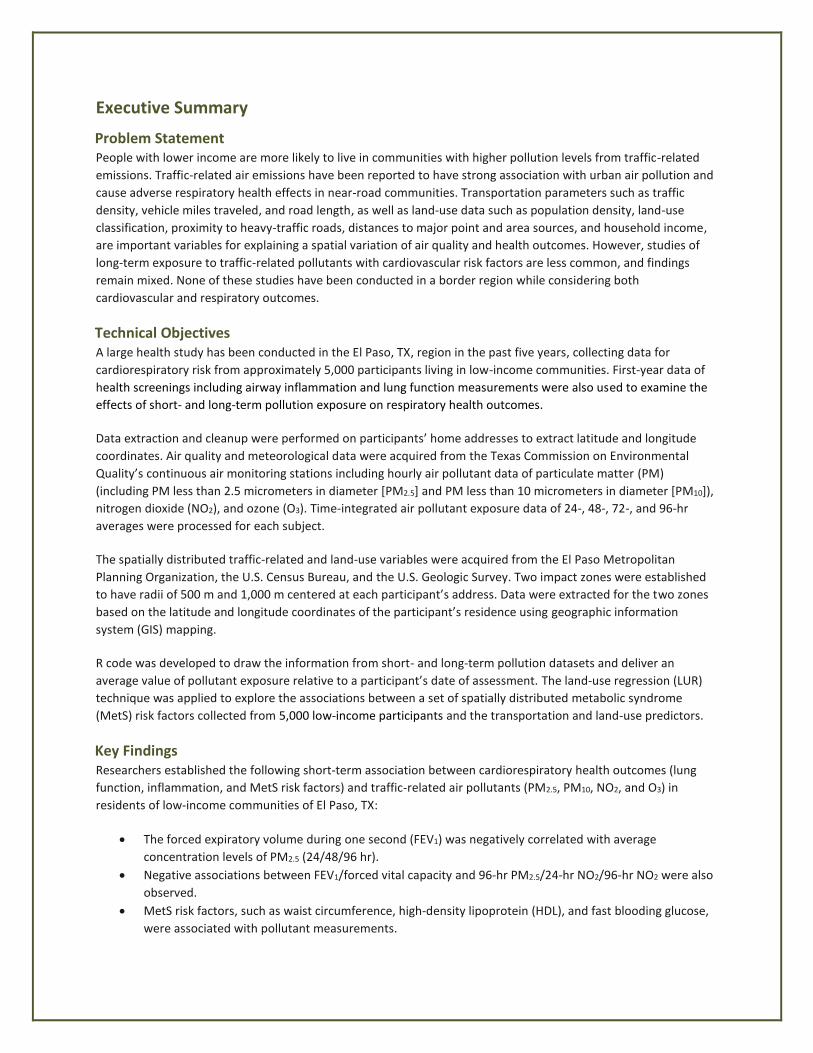
Executive Summary

Problem Statement People with lower income are more likely to live in communities with higher pollution levels from traffic-related

emissions. Traffic-related air emissions have been reported to have strong association with urban air pollution and

cause adverse respiratory health effects in near-road communities. Transportation parameters such as traffic

density, vehicle miles traveled, and road length, as well as land-use data such as population density, land-use

classification, proximity to heavy-traffic roads, distances to major point and area sources, and household income,

are important variables for explaining a spatial variation of air quality and health outcomes. However, studies of

long-term exposure to traffic-related pollutants with cardiovascular risk factors are less common, and findings

remain mixed. None of these studies have been conducted in a border region while considering both

cardiovascular and respiratory outcomes.

Technical Objectives A large health study has been conducted in the El Paso, TX, region in the past five years, collecting data for

cardiorespiratory risk from approximately 5,000 participants living in low-income communities. First-year data of

health screenings including airway inflammation and lung function measurements were also used to examine the

effects of short- and long-term pollution exposure on respiratory health outcomes.

Data extraction and cleanup were performed on participants’ home addresses to extract latitude and longitude

coordinates. Air quality and meteorological data were acquired from the Texas Commission on Environmental

Quality’s continuous air monitoring stations including hourly air pollutant data of particulate matter (PM)

(including PM less than 2.5 micrometers in diameter [PM2.5] and PM less than 10 micrometers in diameter [PM10]),

nitrogen dioxide (NO2), and ozone (O3). Time-integrated air pollutant exposure data of 24-, 48-, 72-, and 96-hr

averages were processed for each subject.

The spatially distributed traffic-related and land-use variables were acquired from the El Paso Metropolitan

Planning Organization, the U.S. Census Bureau, and the U.S. Geologic Survey. Two impact zones were established

to have radii of 500 m and 1,000 m centered at each participant’s address. Data were extracted for the two zones

based on the latitude and longitude coordinates of the participant’s residence using geographic information

system (GIS) mapping.

R code was developed to draw the information from short- and long-term pollution datasets and deliver an

average value of pollutant exposure relative to a participant’s date of assessment. The land-use regression (LUR)

technique was applied to explore the associations between a set of spatially distributed metabolic syndrome

(MetS) risk factors collected from 5,000 low-income participants and the transportation and land-use predictors.

Key Findings Researchers established the following short-term association between cardiorespiratory health outcomes (lung

function, inflammation, and MetS risk factors) and traffic-related air pollutants (PM2.5, PM10, NO2, and O3) in

residents of low-income communities of El Paso, TX:

• The forced expiratory volume during one second (FEV1) was negatively correlated with average

concentration levels of PM2.5 (24/48/96 hr).

• Negative associations between FEV1/forced vital capacity and 96-hr PM2.5/24-hr NO2/96-hr NO2 were also

observed.

• MetS risk factors, such as waist circumference, high-density lipoprotein (HDL), and fast blooding glucose,

were associated with pollutant measurements.

• Waist circumference, in particular, for females is a significant factor showing strong relationships with

PM2.5 and NO2 for all exposure periods.

• Increasing PM2.5 and NO2 concentration was also associated with increasing likelihood of a high waist

circumference.

• A significant relationship between 96-hr averaged O3 and HDL was observed.

• The increase in 24-/48-hr PM2.5 and PM10 were significantly associated with an increase in the box-cox

transformed fasting blood glucose scale. Higher likelihood of having high glucose was associated with

increased PM concentrations.

• The MetS classification based on the combination of five risk factors showed significant associations with

PM2.5, NO2, and O3.

Researchers established the following long-term association between cardiorespiratory health outcomes (lung

function, inflammation, and MetS risk factors) and spatial transportation data for residents of low-income

communities of El Paso, TX:

• The length of the street within the 500-m impact zone has shown to be an important traffic predictor for

lung function (peak expiratory flow [PEF] and the best result interpreted by the spirometry software

(CareFusion Spirometry PC Software™ 36-SPC1000-STK) for PEF [PEF Best].

• The increase in pulse pressure was associated with the amount of traffic within a 500-m radius and the

proximity to the nearest port of entry (POE).

• The increase in the inverse of the distance squared to the POE, which implies a decrease in the distance to

the POE, was significantly associated with an increase in fasting glucose.

• The most significant predictor in the LUR models of MetS risk factors was the total length of the street

within a 500-m radius.

• The increase in the street length associated with increasing waist circumference and triglycerides and

decreasing HDL cholesterol.

• As the total length of the street increases, the risks of a large waist circumference, high triglycerides, and

low HDL cholesterol were observed.

• The increasing likelihood of MetS was also related to the increased street length within 500 m.

Project Impacts Researchers found associations between cardiorespiratory outcomes and traffic-related data for both air quality

and traffic-related activities. Aside from the participants receiving their screening results, this project provides

relevant air quality information to the participants. Spatial variations of environmental and traffic-related data

were informed for the defined impact zones (500 m and 1,000 m). In parallel, this project integrated health

outcome data into a GIS map. A predicted map of MetS was produced to show the prediction of the spatial

distribution of MetS outcome in El Paso, TX. The dissemination of results can lead to decision making and improve

policy related to healthy living in communities close to busy roadways. The research team envisions providing

education regarding the detrimental effects of air pollution, which can be combined with the Healthy Living and

Traffic-Related Air Pollution initiative to improve participants’ health.

vii

Acknowledgments

This research conducted a secondary data analysis that includes low-income participants from El Paso, TX. The

participants were recruited as part of an epidemiological study titled Evidence-Based Screening for Obesity,

Cardiorespiratory Disease, and Environmental Exposures in Low-Income El Paso Households, funded by the City of

El Paso’s Department of Public Health.

The research team would also like to acknowledge significant contributions from Dr. Mayra Chavez from the Civil

Engineering Department and from Dr. Gabriel Ibarra-Mejia and Dr. Joao Ferreira-Pinto from the College of Health

Sciences at The University of Texas at El Paso.

ix

Table of Contents

List of Figures ........................................................................................................................................................ xi

List of Tables ........................................................................................................................................................ xii

List of Acronyms ..................................................................................................................................................xiii

Background and Introduction ................................................................................................................................ 1

Introduction ........................................................................................................................................................... 1

Short-Term Air Pollution Exposure Assessments .................................................................................................... 2

Long-Term Air Pollution Exposure Assessments ..................................................................................................... 2

Limitations of Continuous Ambient Monitoring Stations ....................................................................................... 3

Incorporation of Geographical Information in Models ........................................................................................... 3

Pollution Exposure and Health Outcomes in El Paso, TX ........................................................................................ 3

Approach ............................................................................................................................................................... 5

Respiratory Health Measures ................................................................................................................................ 5

Traffic-Related Measures ....................................................................................................................................... 5

Methodology ......................................................................................................................................................... 9

GIS Mapping .......................................................................................................................................................... 9

Statistical Methods .............................................................................................................................................. 10

Results ................................................................................................................................................................. 11

Short-Term Effects of Traffic-Related Air Pollution on Cardiorespiratory Outcomes ............................................ 11

Demographics ..................................................................................................................................................... 11

Air Pollution Measurements ............................................................................................................................... 12

Respiratory Associations ..................................................................................................................................... 14

Cardiovascular Associations ................................................................................................................................ 19

Long-Term Effects of Transportation Data on Cardiorespiratory Outcomes ......................................................... 33

Demographics ..................................................................................................................................................... 33

Traffic-Related Measurements ........................................................................................................................... 34

Respiratory Associations Using First-Year Subset of Data .................................................................................. 36

Cardiovascular Associations Using First-Year Subset of Data ............................................................................. 40

Cardiovascular Associations Using Five-Year Data.............................................................................................. 46

Predictive Probability Model .............................................................................................................................. 55

Conclusions and Recommendations .................................................................................................................... 58

Short-Term Effects of Traffic-Related Air Pollution on Cardiorespiratory Outcomes ............................................ 58

Strengths and Limitations ................................................................................................................................... 59

Comparison with Other Studies .......................................................................................................................... 59

Long-Term Effects of Transportation Data on Cardiorespiratory Outcomes ......................................................... 59

Strengths and Limitations ................................................................................................................................... 60

x

Comparison with Other Studies .......................................................................................................................... 60

Outputs, Outcomes, and Impacts ......................................................................................................................... 62

Research Outputs, Outcomes, and Impacts ......................................................................................................... 62

Technology Transfer Outputs, Outcomes, and Impacts ........................................................................................ 63

Education and Workforce Development Outputs, Outcomes, and Impacts ......................................................... 63

References ........................................................................................................................................................... 65

xi

List of Figures

Figure 1. Location of CAMSs in El Paso, TX, for selected air pollutants. ........................................................................ 6 Figure 2. Residential addresses of low-income participants from El Paso, TX. ............................................................. 6 Figure 3. Major arterial roads layer. .............................................................................................................................. 7 Figure 4. Ports of entry in El Paso, TX. ........................................................................................................................... 7 Figure 5. Metropolitan planning organization traffic layer and zoomed version. ......................................................... 8 Figure 6. Census.gov street layer and zoomed version. ................................................................................................ 8 Figure 7. Distance to the nearest major arterial (majart) road and majart layer zoom. ............................................... 9 Figure 8. Summary of street length within 500 m using the Census.gov layer. ............................................................ 9 Figure 9. Summary of street length within 500 m using the metropolitan planning organization layer. ................... 10 Figure 10. Summary boxplots of air pollution concentrations. ................................................................................... 14 Figure 11. Scatterplot matrix of pairs of eight traffic variables (N=662). .................................................................... 35 Figure 12. Scatterplot matrix of pairs of eight traffic variables (N=4,959). ................................................................. 36 Figure 13. Traffic-related variables applied to a city grid for (A) street length within 500 m, (B) distance to

the nearest port of entry, and (C) VMT within 500 m. .................................................................................. 56 Figure 14. Predictive model of higher risk of MetS based on the land-use regression model. ................................... 57

xii

List of Tables

Table 1. Demographic Information for Subjects (N=662) ............................................................................................ 11 Table 2. Summary Statistics of Participant Characteristics (N=662) ............................................................................ 12 Table 3. Spatial Distribution of Subjects to the Nearest CAMS (N=662) ..................................................................... 13 Table 4. Summary Statistics for Pollutant Measurements over Various Window Exposures (N=662)........................ 13 Table 5. Descriptive Statistics for eNO, FEV1, FVC, and PEF Metrics (N=662) ............................................................. 14 Table 6. Association between Respiratory Outcome and Pollutant Metrics (N=662) ................................................. 15 Table 7. Descriptive Statistics for MetS Risk Factors (N=662) ..................................................................................... 20 Table 8. Correlation Analysis (N=662) ......................................................................................................................... 20 Table 9. Association between Cardiovascular Outcome and Pollutant Metrics (N=662) ............................................ 22 Table 10. Summary of MetS Risk Factors (N=662)....................................................................................................... 30 Table 11. Associations between MetS Risk Factors and MetS Classification and Pollutant Metrics (N=662) ............. 30 Table 12. Demographic Information for Subjects (N=4,959) ....................................................................................... 33 Table 13. Descriptive Statistics of Traffic Variables (N=662; Unit: km, in Thousands) ................................................ 35 Table 14. Descriptive Statistics of Traffic Variables (N=4,959; Unit: km, in Thousands) ............................................. 36 Table 15. Correlation Analysis between Respiratory Outcome and Traffic Variables (N=662) ................................... 37 Table 16. Summary and Parameter Estimates of Multivariate Regression Models for Respiratory Outcomes

(N=662) .......................................................................................................................................................... 38 Table 17. Correlation Analysis (N=662) ....................................................................................................................... 40 Table 18. Univariate Associations between MetS Risk Factors and MetS Classification and Traffic Variables

(N=662) .......................................................................................................................................................... 41 Table 19. Summary and Parameter Estimates of Multivariate Regression Models for Continuous MetS Risk

Factors (N=662) ............................................................................................................................................. 42 Table 20. Summary and Parameter Estimates of Multivariate Logistic Regression Model for Binary MetS

Factors (N=662) ............................................................................................................................................. 45 Table 21. Descriptive Statistics for MetS Risk Factors (N=4,959) ................................................................................ 47 Table 22. Correlation Analysis (N=4,959) .................................................................................................................... 48 Table 23. Summary of MetS Risk Factors (N=4,959).................................................................................................... 48 Table 24. Univariate Associations between MetS Risk Factors and MetS Classification and Traffic Variables

(N=4,959) ....................................................................................................................................................... 49 Table 25. Summary and Parameter Estimates of Multivariate Regression Models for Continuous MetS Risk

Factors (N=4,959) .......................................................................................................................................... 51 Table 26. Summary and Parameter Estimates of Multivariate Logistic Regression Model for Binary MetS

Factors (N=4,959) .......................................................................................................................................... 54 Table 27. Summary of Variable Selection for Multivariate Logistic Regression Models Using a Stepwise

Selection Technique ...................................................................................................................................... 55

xiii

List of Acronyms

BMI Body mass index BP Blood pressure CAMS Continuous Ambient Monitoring Sites COPD Chronic obstructive pulmonary disease DBP Diastolic blood pressure eNO Exhaled nitric oxide FBG Fasting blood glucose FEF25-75 Forced expiratory flow during the two interior quartiles of exhalation FEV0.5 Forced expiratory volume in half a second FEV1 Forced expiratory volume in one second FVC Forced vital capacity GIS Geographic Information System HbA1c Glycated hemoglobin HDL High-density lipoprotein cholesterol IQR Inter-quartile range LDL Low-density lipoprotein cholesterol LUR Land-use regression MetS Metabolic syndrome NA Not applicable, missing value NO2 Nitrogen dioxide O3 Ozone PBP Pulse blood pressure PEF Peak expiratory flow PM Particulate matter PM2.5 Particle with aerodynamic diameters of less than 2.5 µm PM10 Particle with aerodynamic diameters of less than 10 µm POE Ports of entry Q1 The first quartile Q3 The third quartile SD Standard deviation SBP Systolic blood pressure TC Total cholesterol TCEQ Texas Commission on Environmental Quality TG Triglyceride UTEP University of Texas at El Paso VMT Vehicles miles traveled

1

Background and Introduction

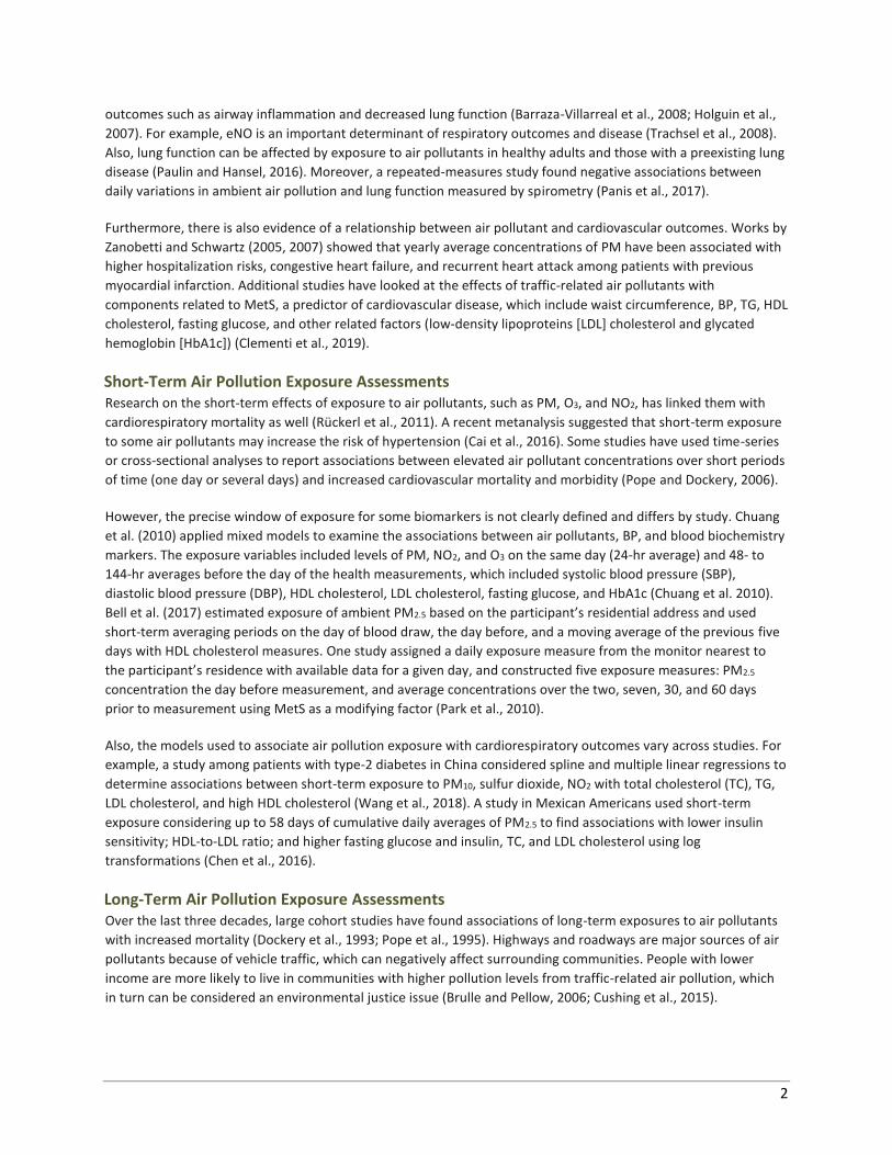
Introduction Air pollution is caused by different pollutants in the atmosphere that can harm living organisms and the natural

environment. The health effects of air pollution from outdoor environments are of great concern due to the high

exposure risk even at relatively low concentrations of air pollutants (Kim et al., 2015). People living in areas with

higher exposure to air pollution compared to those in less polluted areas were more likely to die, and stronger

associations were found with cardiorespiratory deaths (Dockery et al., 1993; Pope et al., 1995). Several scientific

publications have outlined how exposure to these particles is a source of various health problems including heart

and lung disease, irregular heartbeat, aggravated asthma, decreased lung function, and increased respiratory

symptoms (Atkinson et al., 2010; Cadelis et al., 2014; Correia et al., 2013).

In addition, air pollution may promote the development of several cardiovascular risk factors (e.g., elevated lipids

and blood pressure) and lead to type-2 diabetes (Bowe et al., 2018; Pope et al., 2015; Rao et al., 2015). Suggested

mechanisms for this interaction include alteration in pathways for control of adipose tissue, the presence of

particles in the systemic circulation, release of inflammatory mediators, and the effects on glucose metabolism

(Rao et al., 2015; Wellen and Hotamisligil, 2003; Xu et al., 2003). In recent decades, many cardiorespiratory

biomarkers have been identified and studied in relation to air pollution exposure (Rom et al., 2013). Even if not all

biomarkers are in the causal pathway for development of a disease, they can be considered valuable indices of a

change in disease risk of air pollution exposure (Thurston et al., 2017).

Exhaled nitric oxide (eNO) is considered a biomarker of airway/lung inflammation, which is an important

determinant of asthma and other lung diseases (Trachsel et al., 2008). eNO measurements have been adopted in

large epidemiological studies to elucidate the negative impacts of air pollution on pulmonary inflammation in

asthmatic children (Delfino et al., 2006; Holguin et al., 2007; Liu et al., 2009). An elevated eNO value indicates

airway inflammation, which translates to an increase in inflammatory processes such as asthma (Holguin et al.,

2007; Steerenberg et al., 2003). Lung function measurements are assessed by considering the expiratory flow rate

in the amount of time required for a person to exhale. Lung function is usually assessed in terms of forced vital

capacity (FVC), forced expiratory volume in one second (FEV1), peak expiratory flow (PEF), and forced expiratory

flow during the two interior quartiles of exhalation (FEF25-75%) (Hankinson et al., 1999).

Metabolic syndrome (MetS) is a known precursor of cardiovascular disease, hypertension, and type-2 diabetes

(Chen and Schwartz, 2008), and consists of a group of five risk factors:

• Excess abdominal fat.

• High blood pressure (BP).

• High triglyceride (TG) levels.

• Low high-density lipoprotein (HDL) cholesterol (called good cholesterol) levels.

• High fasting glucose.

Having three or more of these risk factors results in a classification of MetS, which, in itself, is a risk factor for

cardiovascular disease, diabetes, hypertension, and dyslipidemia (abnormal lipids). The high prevalence and

increasing number of U.S. adults (34 percent) with MetS has become a public health concern that presents a great

challenge to health care (Mozumdar and Liguori, 2011).

Traffic-related pollutants include particulate matter (PM) (including PM less than 2.5 micrometers in diameter

[PM2.5] and PM less than 10 micrometers in diameter [PM10]), nitrogen dioxide (NO2), and ozone (O3). A recent

review indicated air pollution from traffic sources is a major preventable cause of respiratory disease (Laumbach

and Kipen, 2012). Previous studies have linked the short-term effects of traffic-related pollutants to respiratory

2

outcomes such as airway inflammation and decreased lung function (Barraza-Villarreal et al., 2008; Holguin et al.,

2007). For example, eNO is an important determinant of respiratory outcomes and disease (Trachsel et al., 2008).

Also, lung function can be affected by exposure to air pollutants in healthy adults and those with a preexisting lung

disease (Paulin and Hansel, 2016). Moreover, a repeated-measures study found negative associations between

daily variations in ambient air pollution and lung function measured by spirometry (Panis et al., 2017).

Furthermore, there is also evidence of a relationship between air pollutant and cardiovascular outcomes. Works by

Zanobetti and Schwartz (2005, 2007) showed that yearly average concentrations of PM have been associated with

higher hospitalization risks, congestive heart failure, and recurrent heart attack among patients with previous

myocardial infarction. Additional studies have looked at the effects of traffic-related air pollutants with

components related to MetS, a predictor of cardiovascular disease, which include waist circumference, BP, TG, HDL

cholesterol, fasting glucose, and other related factors (low-density lipoproteins [LDL] cholesterol and glycated

hemoglobin [HbA1c]) (Clementi et al., 2019).

Short-Term Air Pollution Exposure Assessments Research on the short-term effects of exposure to air pollutants, such as PM, O3, and NO2, has linked them with

cardiorespiratory mortality as well (Rückerl et al., 2011). A recent metanalysis suggested that short-term exposure

to some air pollutants may increase the risk of hypertension (Cai et al., 2016). Some studies have used time-series

or cross-sectional analyses to report associations between elevated air pollutant concentrations over short periods

of time (one day or several days) and increased cardiovascular mortality and morbidity (Pope and Dockery, 2006).

However, the precise window of exposure for some biomarkers is not clearly defined and differs by study. Chuang

et al. (2010) applied mixed models to examine the associations between air pollutants, BP, and blood biochemistry

markers. The exposure variables included levels of PM, NO2, and O3 on the same day (24-hr average) and 48- to

144-hr averages before the day of the health measurements, which included systolic blood pressure (SBP),

diastolic blood pressure (DBP), HDL cholesterol, LDL cholesterol, fasting glucose, and HbA1c (Chuang et al. 2010).

Bell et al. (2017) estimated exposure of ambient PM2.5 based on the participant’s residential address and used

short-term averaging periods on the day of blood draw, the day before, and a moving average of the previous five

days with HDL cholesterol measures. One study assigned a daily exposure measure from the monitor nearest to

the participant’s residence with available data for a given day, and constructed five exposure measures: PM2.5

concentration the day before measurement, and average concentrations over the two, seven, 30, and 60 days

prior to measurement using MetS as a modifying factor (Park et al., 2010).

Also, the models used to associate air pollution exposure with cardiorespiratory outcomes vary across studies. For

example, a study among patients with type-2 diabetes in China considered spline and multiple linear regressions to

determine associations between short-term exposure to PM10, sulfur dioxide, NO2 with total cholesterol (TC), TG,

LDL cholesterol, and high HDL cholesterol (Wang et al., 2018). A study in Mexican Americans used short-term

exposure considering up to 58 days of cumulative daily averages of PM2.5 to find associations with lower insulin

sensitivity; HDL-to-LDL ratio; and higher fasting glucose and insulin, TC, and LDL cholesterol using log

transformations (Chen et al., 2016).

Long-Term Air Pollution Exposure Assessments Over the last three decades, large cohort studies have found associations of long-term exposures to air pollutants

with increased mortality (Dockery et al., 1993; Pope et al., 1995). Highways and roadways are major sources of air

pollutants because of vehicle traffic, which can negatively affect surrounding communities. People with lower

income are more likely to live in communities with higher pollution levels from traffic-related air pollution, which

in turn can be considered an environmental justice issue (Brulle and Pellow, 2006; Cushing et al., 2015).

3

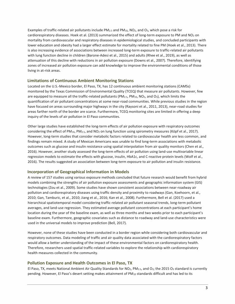
Examples of traffic-related air pollutants include PM2.5 and PM10, NO2, and O3, which pose a risk for

cardiorespiratory diseases. Hoek et al. (2013) summarized the effect of long-term exposure to PM and NO2 on

mortality from cardiovascular and respiratory diseases in epidemiological studies, and concluded participants with

lower education and obesity had a larger effect estimate for mortality related to fine PM (Hoek et al., 2013). There

is also increasing evidence of associations between increased long-term exposure to traffic-related air pollutants

with lung function decline in children (Barone-Adesi et al., 2015) and adults (Rhee et al., 2019), as well as

attenuation of this decline with reductions in air pollution exposure (Downs et al., 2007). Therefore, identifying

zones of increased air pollution exposure can add knowledge to improve the environmental conditions of those

living in at-risk areas.

Limitations of Continuous Ambient Monitoring Stations Located on the U.S.-Mexico border, El Paso, TX, has 12 continuous ambient monitoring stations (CAMSs)

monitored by the Texas Commission of Environmental Quality (TCEQ) that measure air pollutants. However, few

are equipped to measure all the traffic-related pollutants (PM2.5, PM10, NO2, and O3), which limits the

quantification of air pollutant concentrations at some near-road communities. While previous studies in the region

have focused on areas surrounding major highways in the city (Raysoni et al., 2011, 2013), near-road studies for

areas farther north of the border are scarce. Furthermore, TCEQ monitoring sites are limited in offering a deep

inquiry of the levels of air pollution in El Paso communities.

Other large studies have established the long-term effects of air pollution exposure with respiratory outcomes

considering the effect of PM10, PM2.5, and NO2 on lung function using spirometry measures (Köpf et al., 2017).

However, long-term studies that consider metabolic factors related to cardiovascular health are less common, and

findings remain mixed. A study of Mexican Americans was unable to find long-term associations with metabolic

outcomes such as glucose and insulin resistance using spatial interpolation from air quality monitors (Chen et al.,

2016). However, another study assessed the long-term effects of air pollution using land-use multivariable linear

regression models to estimate the effects with glucose, insulin, HbA1c, and C-reactive protein levels (Wolf et al.,

2016). The results suggested an association between long-term exposure to air pollution and insulin resistance.

Incorporation of Geographical Information in Models A review of 157 studies using various exposure methods concluded that future research would benefit from hybrid

models combining the strengths of air pollution exposure assessments and geographic information system (GIS)

technologies (Zou et al., 2009). Some studies have shown consistent associations between near-roadway air

pollution and cardiorespiratory diseases using traffic density and proximity to roadways (Gan, Koehoorn, et al.,

2010; Gan, Tamburic, et al., 2010; Jiang et al., 2016; Kan et al., 2008). Furthermore, Bell et al. (2017) used a

hierarchical spatiotemporal model considering traffic-related air pollutant seasonal trends, long-term pollutant

averages, and land-use regression. They estimated average pollutant concentrations at each participant’s home

location during the year of the baseline exam, as well as three months and two weeks prior to each participant’s

baseline exam. Furthermore, geographic covariates such as distance to roadway and land-use characteristics were

used in the universal models to improve prediction (Bell, 2017).

However, none of these studies have been conducted in a border region while considering both cardiovascular and

respiratory outcomes. Data modeling of traffic and air quality data associated with the cardiorespiratory factors

would allow a better understanding of the impact of these environmental factors on cardiorespiratory health.

Therefore, researchers used spatial traffic-related variables to explore the relationship with cardiorespiratory

health measures collected in the community.

Pollution Exposure and Health Outcomes in El Paso, TX El Paso, TX, meets National Ambient Air Quality Standards for NO2, PM2.5, and O3; the 2015 O3 standard is currently

pending. However, El Paso’s desert setting makes attainment of PM10 standards difficult and has led to its

4

nonattainment classification. The Paso del Norte air basin is shared by El Paso, TX; Ciudad Juarez, Chihuahua; and

Las Cruces, NM. Traffic emissions from the El Paso–Ciudad Juarez border crossings make up a sizable portion of the

mobile vehicle emissions in El Paso.

Previous studies have attempted to characterize the air pollution trends in the Paso del Norte air basin. Industrial

sources, meteorological conditions, and topography were determined to cause variation in the concentration of air

pollutants in the region (Noble et al., 2003). Li et al. (2001) characterized the temporal and spatial variations, along

with the composition of PM. PM10 and PM2.5 were found to increase during the winter months. A study conducted

in 2010 across four schools found that PM10 was greater in the area near I-10 and the El Paso–Ciudad Juarez border

highway (Raysoni et al., 2011). Also, NO2 has been found to be predominate in central El Paso with lower values in

east and west. A winter pilot study showed significant variability in NO2 concentrations across El Paso where NO2

concentrations decreased as elevation increased (Gonzalez et al., 2005).

A large health effect study has been under way in the El Paso region for the past five years that has involved

collecting data for cardiorespiratory risk factors in almost 5,000 participants from low-income communities.

Overall, the Evidence-Based Screening for Obesity, Cardiorespiratory Disease, and Environmental Exposures in

Low-Income El Paso Households project aims to evaluate the overall health status of participants who are of

uninsured/low-income status and to provide health vouchers for further examination for those who qualify.

Individuals who want to participate in the study, which is available to all ages, need to be uninsured/low income

and live within El Paso County.

Health screenings conducted include BP, anthropometric measurements (height, weight, and waist), eNO,

spirometry, fasting glucose, and a lipid profile (TC, TG, HDL, and LDL). The results are given and interpreted with

participants on site. Low-income/free health clinic referrals are given to those with abnormal results. The health

professionals who conducted the health assessments and provided the surveys throughout the study consisted of

physicians, nurses, graduate and undergraduate students from The University of Texas at El Paso (UTEP), and

volunteers. Prevalence rates of each factor have been reported for the first year of the study (N=657) with an

overall prevalence of 53 percent in the selected population (Aguilera, 2016).

Modeling of traffic and air quality data association with the MetS factors allows a better understanding of the

impact of these environmental factors on cardio-metabolic health. This project aims to integrate air quality and

traffic data with large epidemiological study results conducted in the El Paso, TX, region. The main research

question is whether there is an association between the concentration levels of traffic-related air pollutants and

cardiorespiratory-related risk factors. Air quality and meteorological data were acquired from the centralized

TCEQ-operated CAMSs, and the spatial traffic-related variables (e.g., traffic roads, traffic counts, and distances to

ports of entry [POE]) were acquired from the El Paso Metropolitan Planning Organization. The dissemination of

results can lead to decision making and improve policy related to healthy living in communities close to busy

roadways.

5

Approach

This project integrated air quality and traffic-related data with a large epidemiological study conducted in the El

Paso, TX, region, and established a continued partnership for future data collection efforts. The Evidence-Based

Screening for Obesity, Cardiorespiratory Disease, and Environmental Exposures in Low-Income El Paso Households

project is a large, ongoing study that collects data from low-income participants in El Paso, TX. A team of health

professionals conducts a sociodemographic survey and collects health data on site at convenient locations for the

participants. The locations include housing authority communities, faith-based organizations, food distribution

events by local food banks, community health fairs, Mexican Consulate clinic days, and grocery stores, among

others. Data collected include a predictor of cardiovascular risk, MetS, which includes measures of waist

circumference, BP, TG, HDL cholesterol, and fasting glucose. During the baseline year of the study, data collected

also included respiratory measures of airway inflammation (measured by an eNO test) and lung function

(measured by spirometry).

This study conducted a secondary data analysis using health data collected between 2014 and 2020 from the

mentioned large study. The larger study protocol and the amendment for conducting this study have been

approved by the UTEP Institutional Review Board under study numbers 590300-4 and 1249235-3 with a separate

Institutional Review Board review for the secondary analysis under study number 1611345-1

Respiratory Health Measures The study included measures for height, weight (to calculate body mass index [BMI]), waist circumference, BP, a

lipid profile (TG, TC, HDL, and LDL), and fasting glucose. These measures were used to determine the rate of MetS

of the participants. Also, a subset of participants were measured for airway inflammation using a NIOX device to

determine eNO and lung function measured by spirometry (FVC, FEV1, and PEF). Participants included in the study

were residents living within El Paso County recruited in low-income communities.

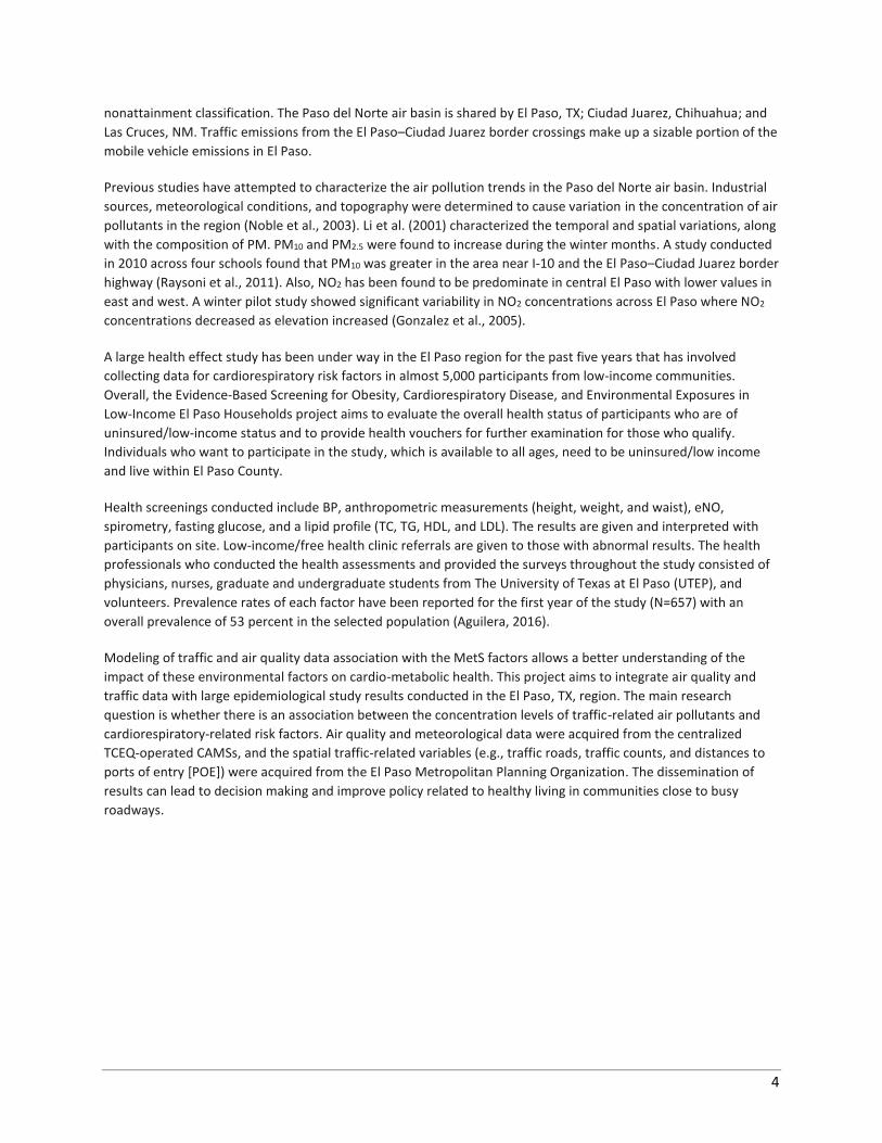
Air pollutants that were continuously measured throughout the study in an outdoor environment included

measurements for PM10, PM2.5, NO2, and O3. The data were extracted using publicly available datasets from CAMSs

maintained by TCEQ. Each participant was assigned to the most representative CAMS based on residential address

(Figure 1). Short-term exposures considered the one-hour average concentration over 24, 48, 72, and 96 hours

before the date of examination for each air pollutant.

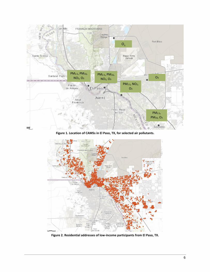
Traffic-Related Measures El Paso, TX, is located in the southwest area of the state and borders with Ciudad Juarez, Mexico, to the south and

Sunland Park, NM, to the west. For this study, researchers considered data from the participant’s home address to

extract latitude and longitude coordinates and create a layer using GIS software (Figure 2).

6

Figure 1. Location of CAMSs in El Paso, TX, for selected air pollutants.

Figure 2. Residential addresses of low-income participants from El Paso, TX.

O3

O3

PM2.5,

PM10, O3

PM2.5, NO2,

O3

PM2.5, PM10,

NO2, O3

PM2.5, PM10,

NO2, O3

7

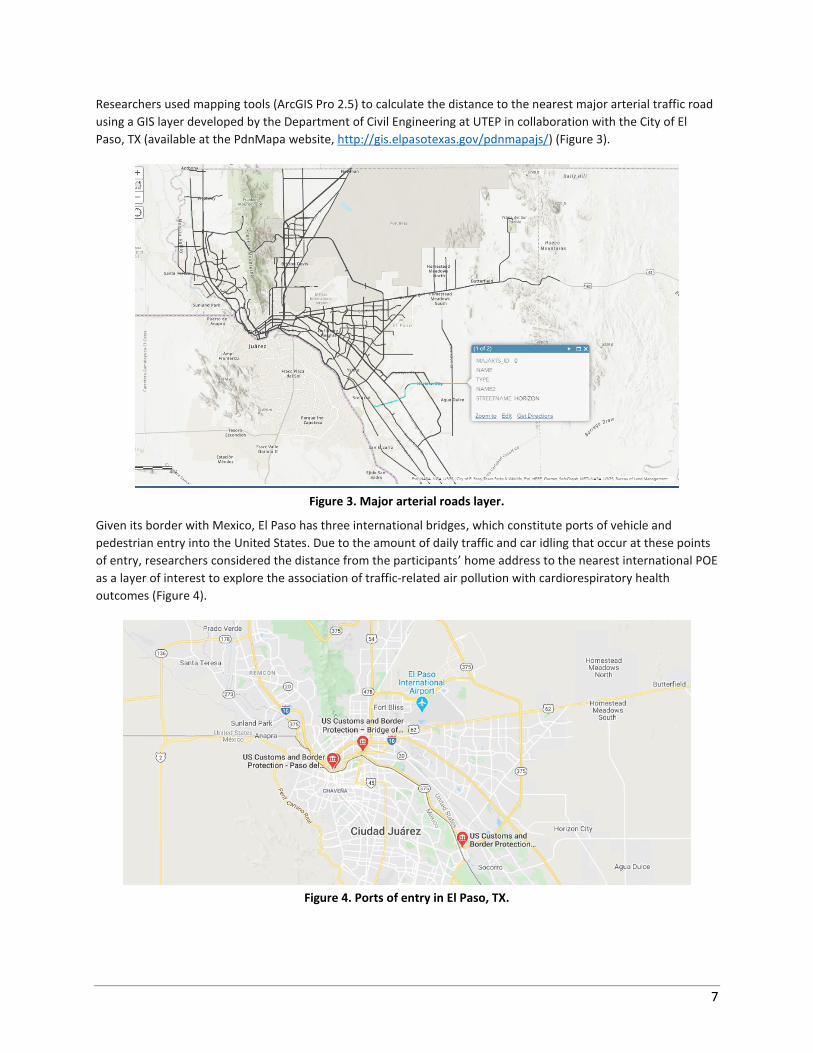
Researchers used mapping tools (ArcGIS Pro 2.5) to calculate the distance to the nearest major arterial traffic road

using a GIS layer developed by the Department of Civil Engineering at UTEP in collaboration with the City of El

Paso, TX (available at the PdnMapa website, http://gis.elpasotexas.gov/pdnmapajs/) (Figure 3).

Figure 3. Major arterial roads layer.

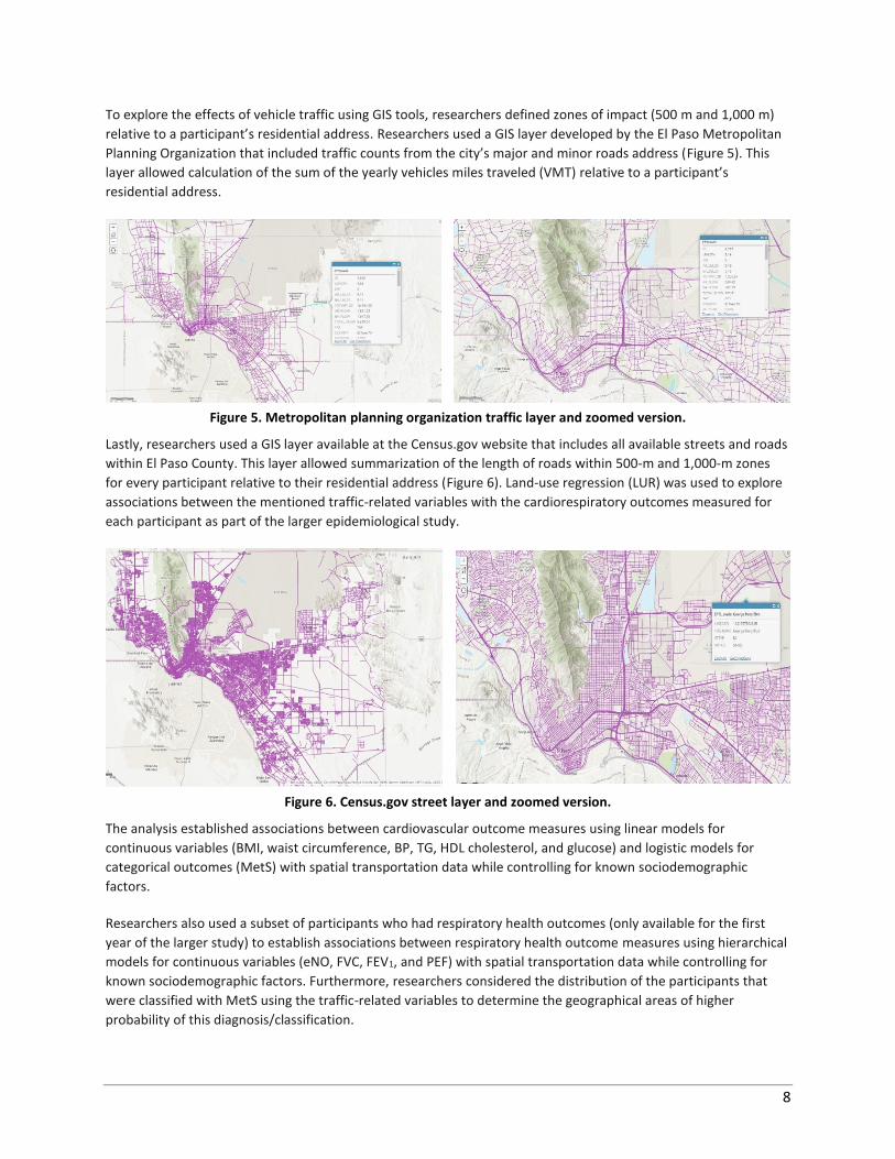
Given its border with Mexico, El Paso has three international bridges, which constitute ports of vehicle and

pedestrian entry into the United States. Due to the amount of daily traffic and car idling that occur at these points

of entry, researchers considered the distance from the participants’ home address to the nearest international POE

as a layer of interest to explore the association of traffic-related air pollution with cardiorespiratory health

outcomes (Figure 4).

Figure 4. Ports of entry in El Paso, TX.

http://gis.elpasotexas.gov/pdnmapajs/

8

To explore the effects of vehicle traffic using GIS tools, researchers defined zones of impact (500 m and 1,000 m)

relative to a participant’s residential address. Researchers used a GIS layer developed by the El Paso Metropolitan

Planning Organization that included traffic counts from the city’s major and minor roads address (Figure 5). This

layer allowed calculation of the sum of the yearly vehicles miles traveled (VMT) relative to a participant’s

residential address.

Figure 5. Metropolitan planning organization traffic layer and zoomed version.

Lastly, researchers used a GIS layer available at the Census.gov website that includes all available streets and roads

within El Paso County. This layer allowed summarization of the length of roads within 500-m and 1,000-m zones

for every participant relative to their residential address (Figure 6). Land-use regression (LUR) was used to explore

associations between the mentioned traffic-related variables with the cardiorespiratory outcomes measured for

each participant as part of the larger epidemiological study.

Figure 6. Census.gov street layer and zoomed version.

The analysis established associations between cardiovascular outcome measures using linear models for

continuous variables (BMI, waist circumference, BP, TG, HDL cholesterol, and glucose) and logistic models for

categorical outcomes (MetS) with spatial transportation data while controlling for known sociodemographic

factors.

Researchers also used a subset of participants who had respiratory health outcomes (only available for the first

year of the larger study) to establish associations between respiratory health outcome measures using hierarchical

models for continuous variables (eNO, FVC, FEV1, and PEF) with spatial transportation data while controlling for

known sociodemographic factors. Furthermore, researchers considered the distribution of the participants that

were classified with MetS using the traffic-related variables to determine the geographical areas of higher

probability of this diagnosis/classification.

9

Methodology

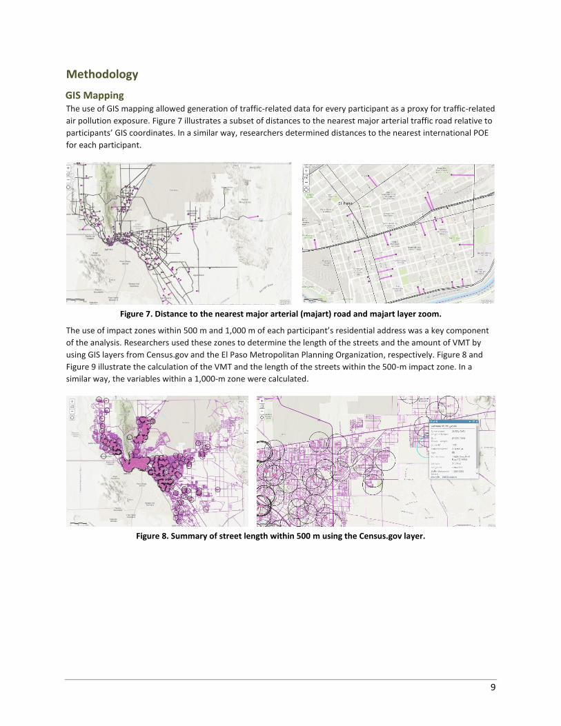
GIS Mapping The use of GIS mapping allowed generation of traffic-related data for every participant as a proxy for traffic-related

air pollution exposure. Figure 7 illustrates a subset of distances to the nearest major arterial traffic road relative to

participants’ GIS coordinates. In a similar way, researchers determined distances to the nearest international POE

for each participant.

Figure 7. Distance to the nearest major arterial (majart) road and majart layer zoom.

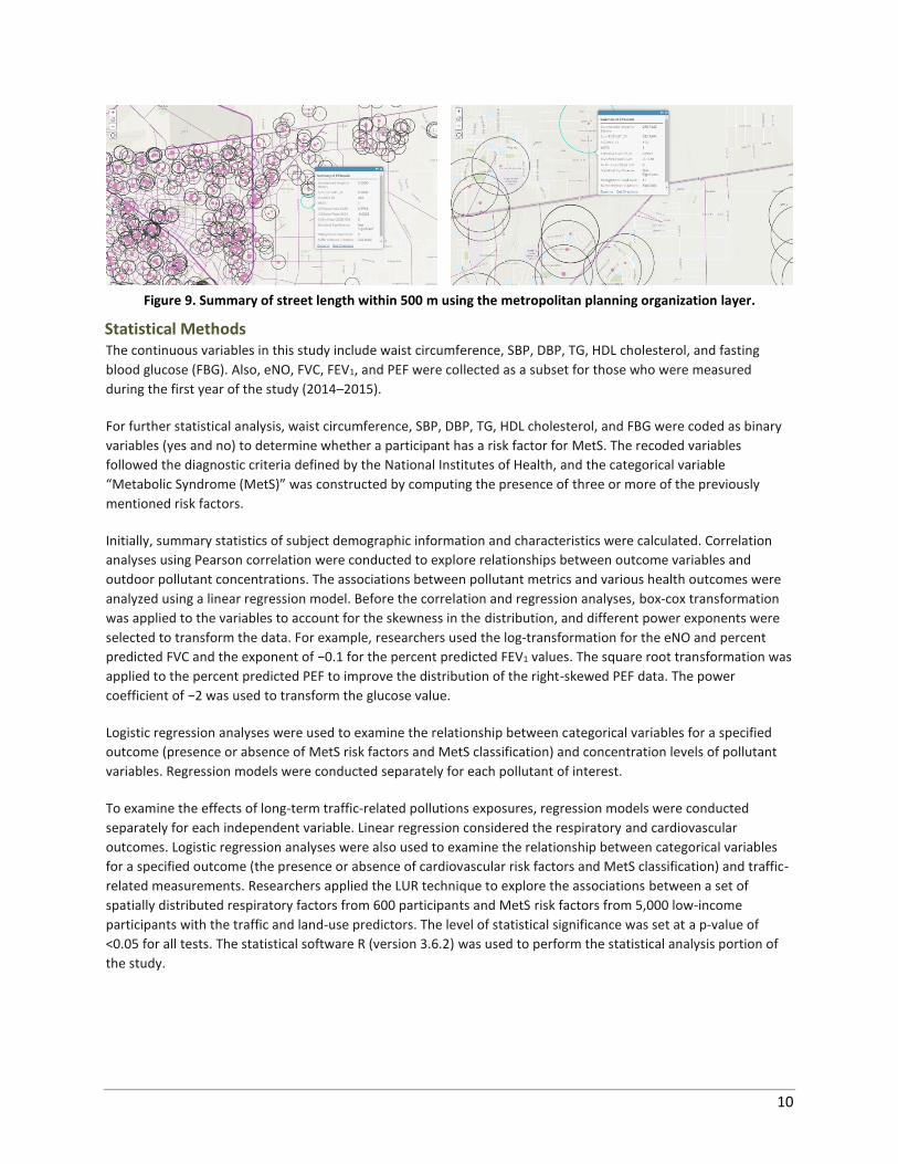
The use of impact zones within 500 m and 1,000 m of each participant’s residential address was a key component

of the analysis. Researchers used these zones to determine the length of the streets and the amount of VMT by

using GIS layers from Census.gov and the El Paso Metropolitan Planning Organization, respectively. Figure 8 and

Figure 9 illustrate the calculation of the VMT and the length of the streets within the 500-m impact zone. In a

similar way, the variables within a 1,000-m zone were calculated.

Figure 8. Summary of street length within 500 m using the Census.gov layer.

10

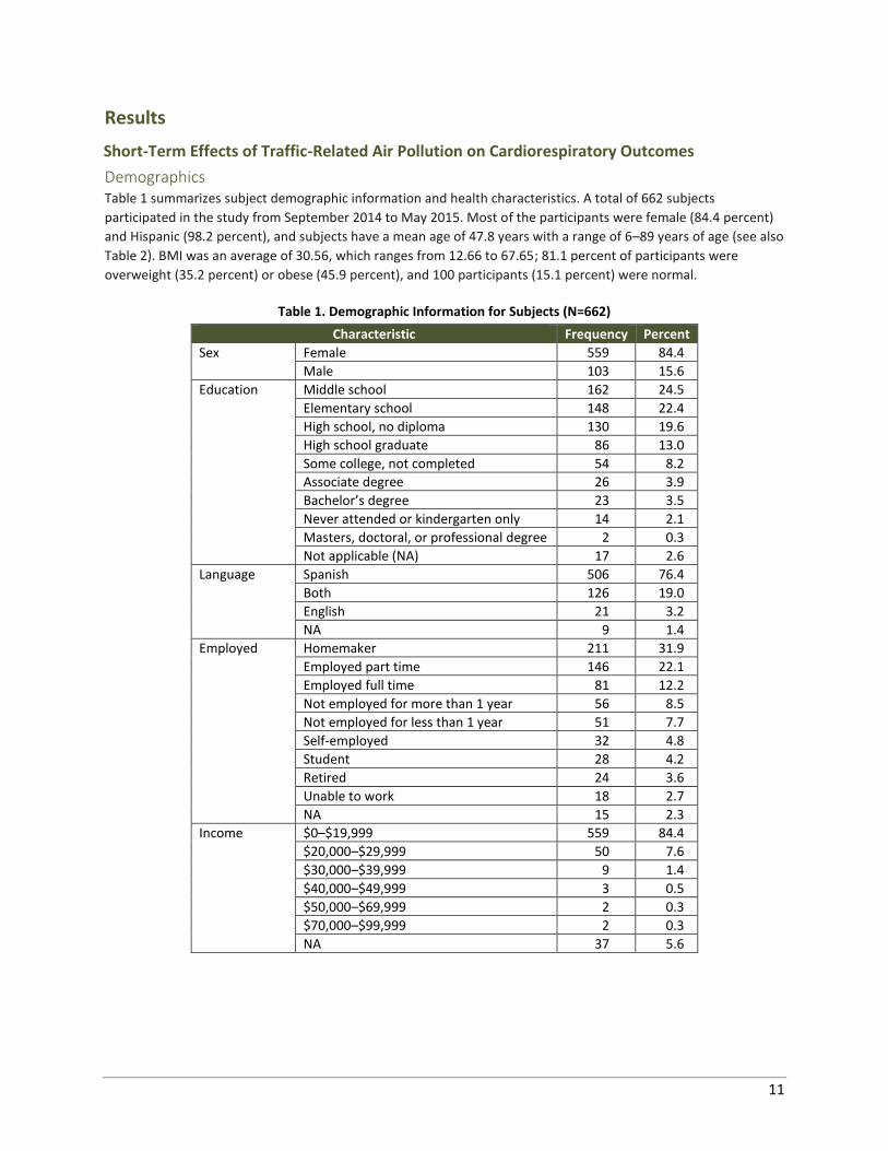
Figure 9. Summary of street length within 500 m using the metropolitan planning organization layer.

Statistical Methods The continuous variables in this study include waist circumference, SBP, DBP, TG, HDL cholesterol, and fasting

blood glucose (FBG). Also, eNO, FVC, FEV1, and PEF were collected as a subset for those who were measured

during the first year of the study (2014–2015).

For further statistical analysis, waist circumference, SBP, DBP, TG, HDL cholesterol, and FBG were coded as binary

variables (yes and no) to determine whether a participant has a risk factor for MetS. The recoded variables

followed the diagnostic criteria defined by the National Institutes of Health, and the categorical variable

“Metabolic Syndrome (MetS)” was constructed by computing the presence of three or more of the previously

mentioned risk factors.

Initially, summary statistics of subject demographic information and characteristics were calculated. Correlation

analyses using Pearson correlation were conducted to explore relationships between outcome variables and

outdoor pollutant concentrations. The associations between pollutant metrics and various health outcomes were

analyzed using a linear regression model. Before the correlation and regression analyses, box-cox transformation

was applied to the variables to account for the skewness in the distribution, and different power exponents were

selected to transform the data. For example, researchers used the log-transformation for the eNO and percent

predicted FVC and the exponent of −0.1 for the percent predicted FEV1 values. The square root transformation was

applied to the percent predicted PEF to improve the distribution of the right-skewed PEF data. The power

coefficient of −2 was used to transform the glucose value.

Logistic regression analyses were used to examine the relationship between categorical variables for a specified

outcome (presence or absence of MetS risk factors and MetS classification) and concentration levels of pollutant

variables. Regression models were conducted separately for each pollutant of interest.

To examine the effects of long-term traffic-related pollutions exposures, regression models were conducted

separately for each independent variable. Linear regression considered the respiratory and cardiovascular

outcomes. Logistic regression analyses were also used to examine the relationship between categorical variables

for a specified outcome (the presence or absence of cardiovascular risk factors and MetS classification) and traffic-

related measurements. Researchers applied the LUR technique to explore the associations between a set of

spatially distributed respiratory factors from 600 participants and MetS risk factors from 5,000 low-income

participants with the traffic and land-use predictors. The level of statistical significance was set at a p-value of

<0.05 for all tests. The statistical software R (version 3.6.2) was used to perform the statistical analysis portion of

the study.

11

Results

Short-Term Effects of Traffic-Related Air Pollution on Cardiorespiratory Outcomes

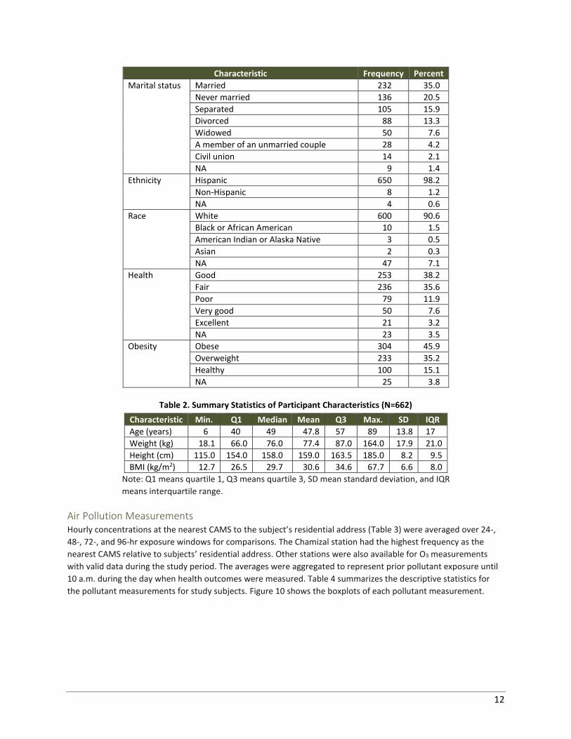
Demographics Table 1 summarizes subject demographic information and health characteristics. A total of 662 subjects

participated in the study from September 2014 to May 2015. Most of the participants were female (84.4 percent)

and Hispanic (98.2 percent), and subjects have a mean age of 47.8 years with a range of 6–89 years of age (see also

Table 2). BMI was an average of 30.56, which ranges from 12.66 to 67.65; 81.1 percent of participants were

overweight (35.2 percent) or obese (45.9 percent), and 100 participants (15.1 percent) were normal.

Table 1. Demographic Information for Subjects (N=662)

Characteristic Frequency Percent

Sex Female 559 84.4

Male 103 15.6

Education Middle school 162 24.5

Elementary school 148 22.4

High school, no diploma 130 19.6

High school graduate 86 13.0

Some college, not completed 54 8.2

Associate degree 26 3.9

Bachelor’s degree 23 3.5

Never attended or kindergarten only 14 2.1

Masters, doctoral, or professional degree 2 0.3

Not applicable (NA) 17 2.6

Language Spanish 506 76.4

Both 126 19.0

English 21 3.2

NA 9 1.4

Employed Homemaker 211 31.9

Employed part time 146 22.1

Employed full time 81 12.2

Not employed for more than 1 year 56 8.5

Not employed for less than 1 year 51 7.7

Self-employed 32 4.8

Student 28 4.2

Retired 24 3.6

Unable to work 18 2.7

NA 15 2.3

Income $0–$19,999 559 84.4

$20,000–$29,999 50 7.6

$30,000–$39,999 9 1.4

$40,000–$49,999 3 0.5

$50,000–$69,999 2 0.3

$70,000–$99,999 2 0.3

NA 37 5.6

12


Marital status Married 232 35.0

Never married 136 20.5

Separated 105 15.9

Divorced 88 13.3

Widowed 50 7.6

A member of an unmarried couple 28 4.2

Civil union 14 2.1

NA 9 1.4

Ethnicity

Hispanic 650 98.2

Non-Hispanic 8 1.2

NA 4 0.6

Race

White 600 90.6

Black or African American 10 1.5

American Indian or Alaska Native 3 0.5

Asian 2 0.3

NA 47 7.1

Health Good 253 38.2

Fair 236 35.6

Poor 79 11.9

Very good 50 7.6

Excellent 21 3.2

NA 23 3.5

Obesity

Obese 304 45.9

Overweight 233 35.2

Healthy 100 15.1

NA 25 3.8

Table 2. Summary Statistics of Participant Characteristics (N=662)

Characteristic Min. Q1 Median Mean Q3 Max. SD IQR

Age (years) 6 40 49 47.8 57 89 13.8 17

Weight (kg) 18.1 66.0 76.0 77.4 87.0 164.0 17.9 21.0

Height (cm) 115.0 154.0 158.0 159.0 163.5 185.0 8.2 9.5

BMI (kg/m2) 12.7 26.5 29.7 30.6 34.6 67.7 6.6 8.0

Note: Q1 means quartile 1, Q3 means quartile 3, SD mean standard deviation, and IQR

means interquartile range.

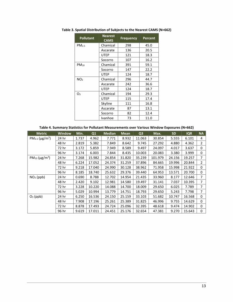
Air Pollution Measurements Hourly concentrations at the nearest CAMS to the subject’s residential address (Table 3) were averaged over 24-,

48-, 72-, and 96-hr exposure windows for comparisons. The Chamizal station had the highest frequency as the

nearest CAMS relative to subjects’ residential address. Other stations were also available for O3 measurements

with valid data during the study period. The averages were aggregated to represent prior pollutant exposure until

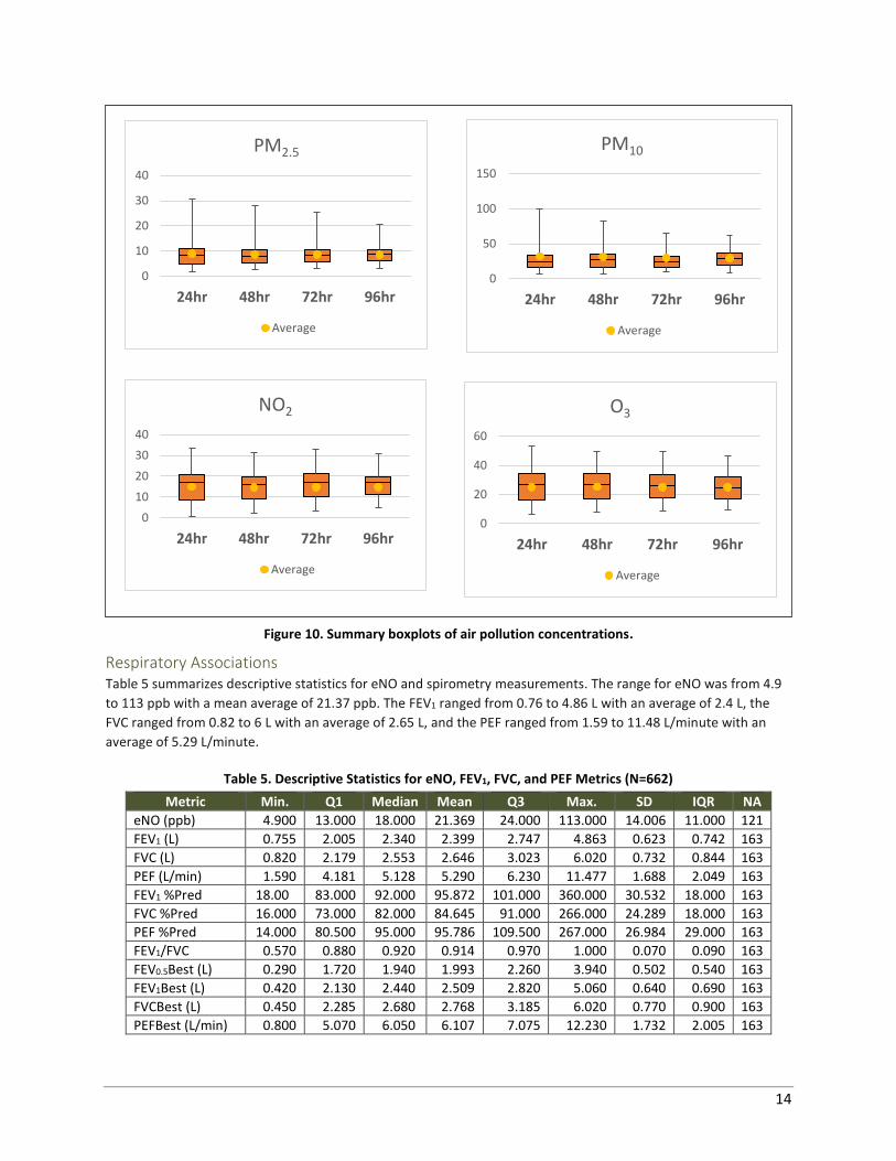
10 a.m. during the day when health outcomes were measured. Table 4 summarizes the descriptive statistics for

the pollutant measurements for study subjects. Figure 10 shows the boxplots of each pollutant measurement.

13

Table 3. Spatial Distribution of Subjects to the Nearest CAMS (N=662)

Pollutant Nearest CAMS

Frequency Percent

PM2.5 Chamizal 298 45.0

Ascarate 136 20.5

UTEP 121 18.3

Socorro 107 16.2

PM10 Chamizal 391 59.1

Socorro 147 22.2

UTEP 124 18.7

NO2 Chamizal 296 44.7

Ascarate 242 36.6

UTEP 124 18.7

O3 Chamizal 194 29.3

UTEP 115 17.4

Skyline 111 16.8

Ascarate 87 13.1

Socorro 82 12.4

Ivanhoe 73 11.0

Table 4. Summary Statistics for Pollutant Measurements over Various Window Exposures (N=662)

Metric Window Min. Q1 Median Mean Q3 Max. SD IQR NA

PM2.5 (μg/m3) 24 hr 1.737 4.962 7.771 8.932 11.063 30.854 5.555 6.101 4

48 hr 2.819 5.382 7.849 8.642 9.745 27.292 4.880 4.362 2

72 hr 3.172 5.859 7.949 8.589 9.497 24.097 4.017 3.637 0

96 hr 3.174 6.003 7.844 8.435 10.003 20.083 3.380 3.999 0

PM10 (μg/m3) 24 hr 7.268 15.982 24.854 31.820 35.239 101.979 24.156 19.257 7

48 hr 6.224 17.052 24.374 31.259 37.896 84.665 19.996 20.844 2

72 hr 9.218 17.040 24.990 30.128 38.962 71.958 15.998 21.922 0

96 hr 8.185 18.740 25.632 29.376 39.440 64.953 13.571 20.700 0

NO2 (ppb) 24 hr 0.690 8.788 12.702 14.954 21.435 33.960 8.177 12.646 7

48 hr 2.420 9.102 12.981 14.580 19.497 31.141 7.037 10.395 7

72 hr 3.228 10.220 14.088 14.700 18.009 29.650 6.025 7.789 7

96 hr 5.029 10.994 13.779 14.751 18.793 29.650 5.243 7.798 7

O3 (ppb) 24 hr 6.250 16.536 24.150 25.159 33.103 51.682 10.747 16.568 0

48 hr 7.908 17.196 25.261 25.389 31.825 46.996 9.755 14.629 0

72 hr 8.878 17.493 24.724 25.096 32.395 48.618 9.474 14.902 0

96 hr 9.619 17.011 24.451 25.176 32.654 47.381 9.270 15.643 0

14

Figure 10. Summary boxplots of air pollution concentrations.

Respiratory Associations Table 5 summarizes descriptive statistics for eNO and spirometry measurements. The range for eNO was from 4.9

to 113 ppb with a mean average of 21.37 ppb. The FEV1 ranged from 0.76 to 4.86 L with an average of 2.4 L, the

FVC ranged from 0.82 to 6 L with an average of 2.65 L, and the PEF ranged from 1.59 to 11.48 L/minute with an

average of 5.29 L/minute.

Table 5. Descriptive Statistics for eNO, FEV1, FVC, and PEF Metrics (N=662)

Metric Min. Q1 Median Mean Q3 Max. SD IQR NA

eNO (ppb) 4.900 13.000 18.000 21.369 24.000 113.000 14.006 11.000 121

FEV1 (L) 0.755 2.005 2.340 2.399 2.747 4.863 0.623 0.742 163

FVC (L) 0.820 2.179 2.553 2.646 3.023 6.020 0.732 0.844 163

PEF (L/min) 1.590 4.181 5.128 5.290 6.230 11.477 1.688 2.049 163

FEV1 %Pred 18.00 83.000 92.000 95.872 101.000 360.000 30.532 18.000 163

FVC %Pred 16.000 73.000 82.000 84.645 91.000 266.000 24.289 18.000 163

PEF %Pred 14.000 80.500 95.000 95.786 109.500 267.000 26.984 29.000 163

FEV1/FVC 0.570 0.880 0.920 0.914 0.970 1.000 0.070 0.090 163

FEV0.5Best (L) 0.290 1.720 1.940 1.993 2.260 3.940 0.502 0.540 163

FEV1Best (L) 0.420 2.130 2.440 2.509 2.820 5.060 0.640 0.690 163

FVCBest (L) 0.450 2.285 2.680 2.768 3.185 6.020 0.770 0.900 163

PEFBest (L/min) 0.800 5.070 6.050 6.107 7.075 12.230 1.732 2.005 163

0

10

20

30

40

24hr 48hr 72hr 96hr

PM2.5

Average

0

50

100

150

24hr 48hr 72hr 96hr

PM10

Average

0

10

20

30

40

24hr 48hr 72hr 96hr

NO2

Average

0

20

40

60

24hr 48hr 72hr 96hr

O3

Average

15

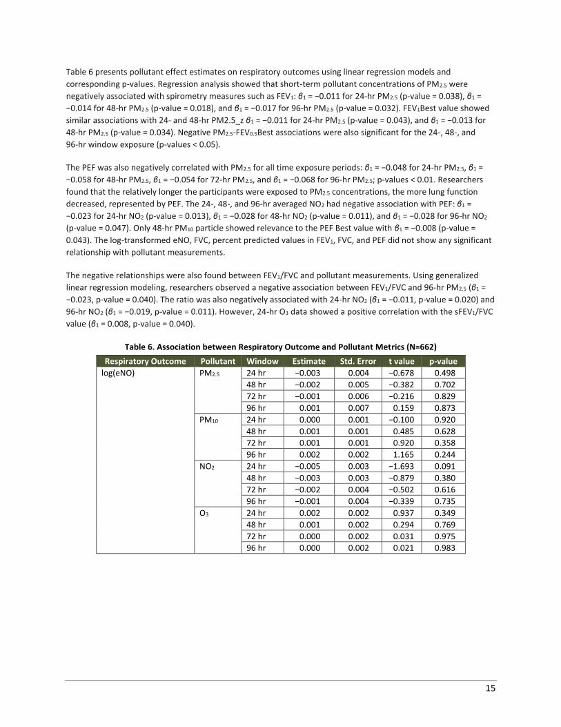
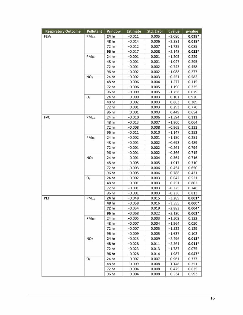
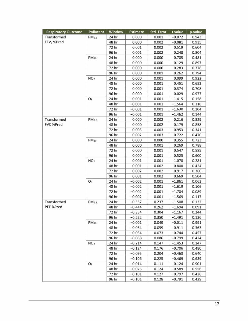
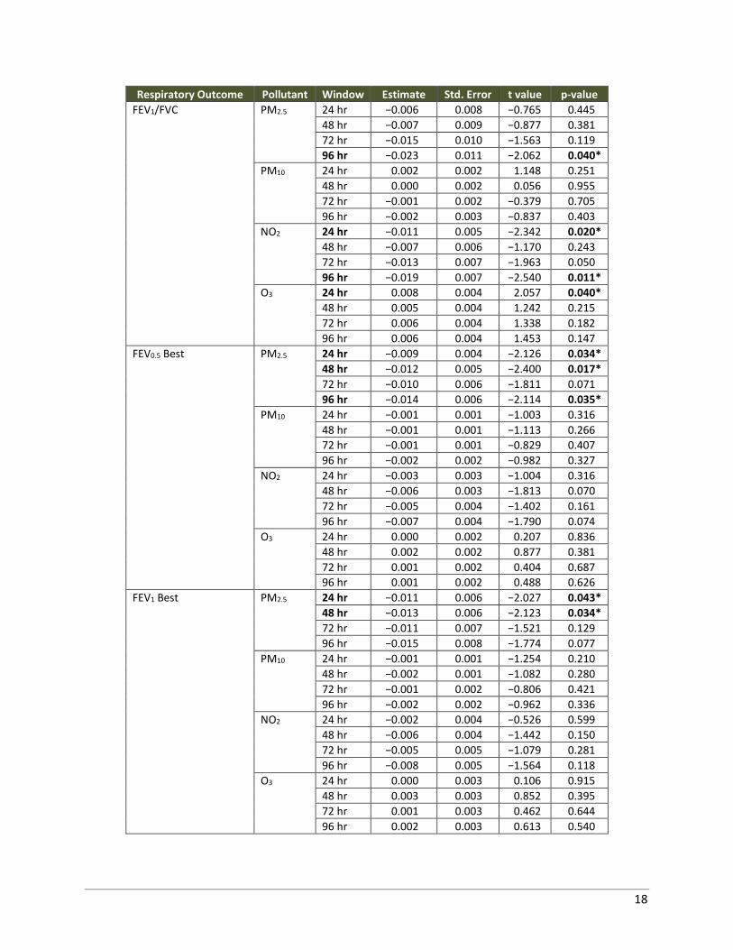
Table 6 presents pollutant effect estimates on respiratory outcomes using linear regression models and

corresponding p-values. Regression analysis showed that short-term pollutant concentrations of PM2.5 were

negatively associated with spirometry measures such as FEV1: β1 = −0.011 for 24-hr PM2.5 (p-value = 0.038), β1 =

−0.014 for 48-hr PM2.5 (p-value = 0.018), and β1 = −0.017 for 96-hr PM2.5 (p-value = 0.032). FEV1Best value showed

similar associations with 24- and 48-hr PM2.5_z β1 = −0.011 for 24-hr PM2.5 (p-value = 0.043), and β1 = −0.013 for

48-hr PM2.5 (p-value = 0.034). Negative PM2.5-FEV0.5Best associations were also significant for the 24-, 48-, and

96-hr window exposure (p-values < 0.05).

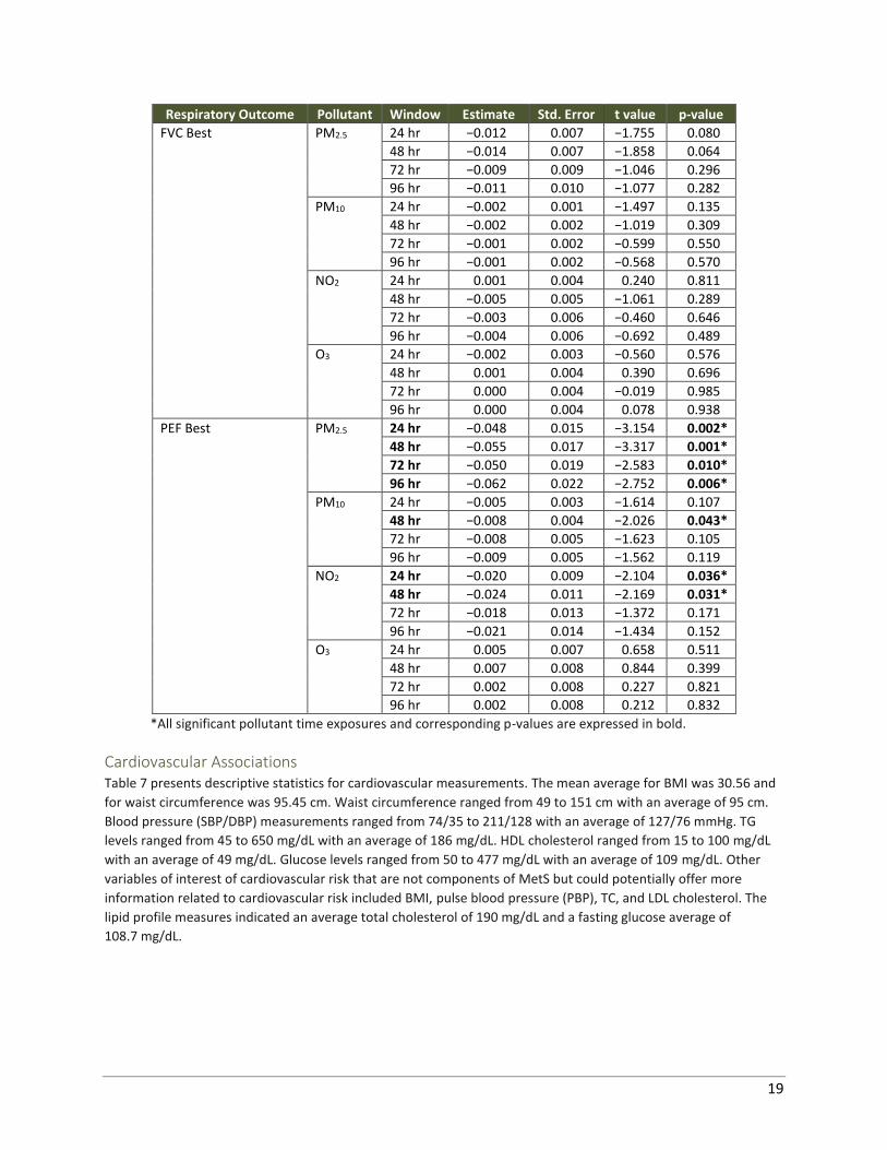
The PEF was also negatively correlated with PM2.5 for all time exposure periods: β1 = −0.048 for 24-hr PM2.5, β1 =

−0.058 for 48-hr PM2.5, β1 = −0.054 for 72-hr PM2.5, and β1 = −0.068 for 96-hr PM2.5; p-values < 0.01. Researchers

found that the relatively longer the participants were exposed to PM2.5 concentrations, the more lung function

decreased, represented by PEF. The 24-, 48-, and 96-hr averaged NO2 had negative association with PEF: β1 =

−0.023 for 24-hr NO2 (p-value = 0.013), β1 = −0.028 for 48-hr NO2 (p-value = 0.011), and β1 = −0.028 for 96-hr NO2

(p-value = 0.047). Only 48-hr PM10 particle showed relevance to the PEF Best value with β1 = −0.008 (p-value =

0.043). The log-transformed eNO, FVC, percent predicted values in FEV1, FVC, and PEF did not show any significant

relationship with pollutant measurements.

The negative relationships were also found between FEV1/FVC and pollutant measurements. Using generalized

linear regression modeling, researchers observed a negative association between FEV1/FVC and 96-hr PM2.5 (β1 =

−0.023, p-value = 0.040). The ratio was also negatively associated with 24-hr NO2 (β1 = −0.011, p-value = 0.020) and

96-hr NO2 (β1 = −0.019, p-value = 0.011). However, 24-hr O3 data showed a positive correlation with the sFEV1/FVC

value (β1 = 0.008, p-value = 0.040).

Table 6. Association between Respiratory Outcome and Pollutant Metrics (N=662)

Respiratory Outcome Pollutant Window Estimate Std. Error t value p-value

log(eNO) PM2.5 24 hr −0.003 0.004 −0.678 0.498

48 hr −0.002 0.005 −0.382 0.702

72 hr −0.001 0.006 −0.216 0.829

96 hr 0.001 0.007 0.159 0.873

PM10 24 hr 0.000 0.001 −0.100 0.920

48 hr 0.001 0.001 0.485 0.628

72 hr 0.001 0.001 0.920 0.358

96 hr 0.002 0.002 1.165 0.244

NO2 24 hr −0.005 0.003 −1.693 0.091

48 hr −0.003 0.003 −0.879 0.380

72 hr −0.002 0.004 −0.502 0.616

96 hr −0.001 0.004 −0.339 0.735

O3 24 hr 0.002 0.002 0.937 0.349

48 hr 0.001 0.002 0.294 0.769

72 hr 0.000 0.002 0.031 0.975

96 hr 0.000 0.002 0.021 0.983

16


FEV1 PM2.5 24 hr −0.011 0.005 −2.080 0.038*

48 hr −0.014 0.006 −2.381 0.018*

72 hr −0.012 0.007 −1.725 0.085

96 hr −0.017 0.008 −2.148 0.032*

PM10 24 hr −0.001 0.001 −1.205 0.229

48 hr −0.001 0.001 −1.047 0.295

72 hr −0.001 0.002 −0.743 0.458

96 hr −0.002 0.002 −1.088 0.277

NO2 24 hr −0.002 0.003 −0.551 0.582

48 hr −0.006 0.004 −1.577 0.115

72 hr −0.006 0.005 −1.190 0.235

96 hr −0.009 0.005 −1.758 0.079

O3 24 hr 0.000 0.003 0.101 0.920

48 hr 0.002 0.003 0.863 0.389

72 hr 0.001 0.003 0.293 0.770

96 hr 0.001 0.003 0.449 0.654

FVC PM2.5 24 hr −0.010 0.006 −1.594 0.111

48 hr −0.013 0.007 −1.860 0.064

72 hr −0.008 0.008 −0.969 0.333

96 hr −0.011 0.010 −1.147 0.252

PM10 24 hr −0.002 0.001 −1.150 0.251

48 hr −0.001 0.002 −0.693 0.489

72 hr −0.001 0.002 −0.261 0.794

96 hr −0.001 0.002 −0.366 0.715

NO2 24 hr 0.001 0.004 0.364 0.716

48 hr −0.005 0.005 −1.017 0.310

72 hr −0.003 0.006 −0.454 0.650

96 hr −0.005 0.006 −0.788 0.431

O3 24 hr −0.002 0.003 −0.642 0.521

48 hr 0.001 0.003 0.251 0.802

72 hr −0.001 0.003 −0.325 0.746

96 hr −0.001 0.003 −0.236 0.813

PEF PM2.5 24 hr −0.048 0.015 −3.289 0.001*

48 hr −0.058 0.016 −3.555 0.000*

72 hr −0.054 0.019 −2.883 0.004*

96 hr −0.068 0.022 −3.120 0.002*

PM10 24 hr −0.005 0.003 −1.509 0.132

48 hr −0.007 0.004 −1.964 0.050

72 hr −0.007 0.005 −1.522 0.129

96 hr −0.009 0.005 −1.637 0.102

NO2 24 hr −0.023 0.009 −2.496 0.013*

48 hr −0.028 0.011 −2.561 0.011*

72 hr −0.023 0.013 −1.787 0.075

96 hr −0.028 0.014 −1.987 0.047*

O3 24 hr 0.007 0.007 0.961 0.337

48 hr 0.009 0.008 1.148 0.251

72 hr 0.004 0.008 0.475 0.635

96 hr 0.004 0.008 0.534 0.593

17


Transformed FEV1 %Pred

PM2.5 24 hr 0.000 0.001 −0.072 0.943

48 hr 0.000 0.002 −0.081 0.935

72 hr 0.001 0.002 0.519 0.604

96 hr 0.001 0.002 0.248 0.804

PM10 24 hr 0.000 0.000 0.705 0.481

48 hr 0.000 0.000 0.129 0.897

72 hr 0.000 0.000 0.283 0.778

96 hr 0.000 0.001 0.262 0.794

NO2 24 hr 0.000 0.001 0.099 0.922

48 hr 0.000 0.001 0.451 0.652

72 hr 0.000 0.001 0.374 0.708

96 hr 0.000 0.001 0.029 0.977

O3 24 hr −0.001 0.001 −1.415 0.158

48 hr −0.001 0.001 −1.564 0.118

72 hr −0.001 0.001 −1.630 0.104

96 hr −0.001 0.001 −1.462 0.144

Transformed FVC %Pred

PM2.5 24 hr 0.000 0.002 0.216 0.829

48 hr 0.000 0.002 0.179 0.858

72 hr 0.003 0.003 0.953 0.341

96 hr 0.002 0.003 0.722 0.470

PM10 24 hr 0.000 0.000 0.355 0.723

48 hr 0.000 0.001 0.269 0.788

72 hr 0.000 0.001 0.547 0.585

96 hr 0.000 0.001 0.525 0.600

NO2 24 hr 0.001 0.001 1.078 0.281

48 hr 0.001 0.002 0.800 0.424

72 hr 0.002 0.002 0.917 0.360

96 hr 0.001 0.002 0.669 0.504

O3 24 hr −0.002 0.001 −1.861 0.063

48 hr −0.002 0.001 −1.619 0.106

72 hr −0.002 0.001 −1.704 0.089

96 hr −0.002 0.001 −1.569 0.117

Transformed PEF %Pred

PM2.5 24 hr −0.357 0.237 −1.508 0.132

48 hr −0.444 0.262 −1.694 0.091

72 hr −0.354 0.304 −1.167 0.244

96 hr −0.522 0.350 −1.491 0.136

PM10 24 hr −0.001 0.049 −0.011 0.991

48 hr −0.054 0.059 −0.911 0.363

72 hr −0.054 0.073 −0.744 0.457

96 hr −0.068 0.086 −0.799 0.424

NO2 24 hr −0.214 0.147 −1.453 0.147

48 hr −0.124 0.176 −0.706 0.480

72 hr −0.095 0.204 −0.468 0.640

96 hr −0.106 0.225 −0.469 0.639

O3 24 hr −0.014 0.111 −0.124 0.901

48 hr −0.073 0.124 −0.589 0.556

72 hr −0.101 0.127 −0.797 0.426

96 hr −0.101 0.128 −0.791 0.429

18


FEV1/FVC PM2.5 24 hr −0.006 0.008 −0.765 0.445

48 hr −0.007 0.009 −0.877 0.381

72 hr −0.015 0.010 −1.563 0.119

96 hr −0.023 0.011 −2.062 0.040*

PM10 24 hr 0.002 0.002 1.148 0.251

48 hr 0.000 0.002 0.056 0.955

72 hr −0.001 0.002 −0.379 0.705

96 hr −0.002 0.003 −0.837 0.403

NO2 24 hr −0.011 0.005 −2.342 0.020*

48 hr −0.007 0.006 −1.170 0.243

72 hr −0.013 0.007 −1.963 0.050

96 hr −0.019 0.007 −2.540 0.011*

O3 24 hr 0.008 0.004 2.057 0.040*

48 hr 0.005 0.004 1.242 0.215

72 hr 0.006 0.004 1.338 0.182

96 hr 0.006 0.004 1.453 0.147

FEV0.5 Best PM2.5 24 hr −0.009 0.004 −2.126 0.034*

48 hr −0.012 0.005 −2.400 0.017*

72 hr −0.010 0.006 −1.811 0.071

96 hr −0.014 0.006 −2.114 0.035*

PM10 24 hr −0.001 0.001 −1.003 0.316

48 hr −0.001 0.001 −1.113 0.266

72 hr −0.001 0.001 −0.829 0.407

96 hr −0.002 0.002 −0.982 0.327

NO2 24 hr −0.003 0.003 −1.004 0.316

48 hr −0.006 0.003 −1.813 0.070

72 hr −0.005 0.004 −1.402 0.161

96 hr −0.007 0.004 −1.790 0.074

O3 24 hr 0.000 0.002 0.207 0.836

48 hr 0.002 0.002 0.877 0.381

72 hr 0.001 0.002 0.404 0.687

96 hr 0.001 0.002 0.488 0.626

FEV1 Best PM2.5 24 hr −0.011 0.006 −2.027 0.043*

48 hr −0.013 0.006 −2.123 0.034*

72 hr −0.011 0.007 −1.521 0.129

96 hr −0.015 0.008 −1.774 0.077

PM10 24 hr −0.001 0.001 −1.254 0.210

48 hr −0.002 0.001 −1.082 0.280

72 hr −0.001 0.002 −0.806 0.421

96 hr −0.002 0.002 −0.962 0.336

NO2 24 hr −0.002 0.004 −0.526 0.599

48 hr −0.006 0.004 −1.442 0.150

72 hr −0.005 0.005 −1.079 0.281

96 hr −0.008 0.005 −1.564 0.118

O3 24 hr 0.000 0.003 0.106 0.915

48 hr 0.003 0.003 0.852 0.395

72 hr 0.001 0.003 0.462 0.644

96 hr 0.002 0.003 0.613 0.540

19


FVC Best PM2.5 24 hr −0.012 0.007 −1.755 0.080

48 hr −0.014 0.007 −1.858 0.064

72 hr −0.009 0.009 −1.046 0.296

96 hr −0.011 0.010 −1.077 0.282

PM10 24 hr −0.002 0.001 −1.497 0.135

48 hr −0.002 0.002 −1.019 0.309

72 hr −0.001 0.002 −0.599 0.550

96 hr −0.001 0.002 −0.568 0.570

NO2 24 hr 0.001 0.004 0.240 0.811

48 hr −0.005 0.005 −1.061 0.289

72 hr −0.003 0.006 −0.460 0.646

96 hr −0.004 0.006 −0.692 0.489

O3 24 hr −0.002 0.003 −0.560 0.576

48 hr 0.001 0.004 0.390 0.696

72 hr 0.000 0.004 −0.019 0.985

96 hr 0.000 0.004 0.078 0.938

PEF Best PM2.5 24 hr −0.048 0.015 −3.154 0.002*

48 hr −0.055 0.017 −3.317 0.001*

72 hr −0.050 0.019 −2.583 0.010*

96 hr −0.062 0.022 −2.752 0.006*

PM10 24 hr −0.005 0.003 −1.614 0.107

48 hr −0.008 0.004 −2.026 0.043*

72 hr −0.008 0.005 −1.623 0.105

96 hr −0.009 0.005 −1.562 0.119

NO2 24 hr −0.020 0.009 −2.104 0.036*

48 hr −0.024 0.011 −2.169 0.031*

72 hr −0.018 0.013 −1.372 0.171

96 hr −0.021 0.014 −1.434 0.152

O3 24 hr 0.005 0.007 0.658 0.511

48 hr 0.007 0.008 0.844 0.399

72 hr 0.002 0.008 0.227 0.821

96 hr 0.002 0.008 0.212 0.832

*All significant pollutant time exposures and corresponding p-values are expressed in bold.

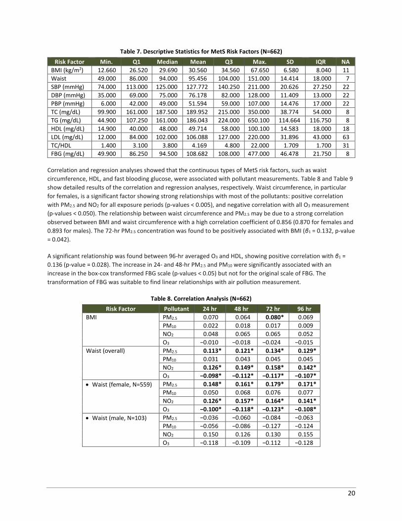
Cardiovascular Associations Table 7 presents descriptive statistics for cardiovascular measurements. The mean average for BMI was 30.56 and

for waist circumference was 95.45 cm. Waist circumference ranged from 49 to 151 cm with an average of 95 cm.

Blood pressure (SBP/DBP) measurements ranged from 74/35 to 211/128 with an average of 127/76 mmHg. TG

levels ranged from 45 to 650 mg/dL with an average of 186 mg/dL. HDL cholesterol ranged from 15 to 100 mg/dL

with an average of 49 mg/dL. Glucose levels ranged from 50 to 477 mg/dL with an average of 109 mg/dL. Other

variables of interest of cardiovascular risk that are not components of MetS but could potentially offer more

information related to cardiovascular risk included BMI, pulse blood pressure (PBP), TC, and LDL cholesterol. The

lipid profile measures indicated an average total cholesterol of 190 mg/dL and a fasting glucose average of

108.7 mg/dL.

20

Table 7. Descriptive Statistics for MetS Risk Factors (N=662)

Risk Factor Min. Q1 Median Mean Q3 Max. SD IQR NA

BMI (kg/m2) 12.660 26.520 29.690 30.560 34.560 67.650 6.580 8.040 11

Waist 49.000 86.000 94.000 95.456 104.000 151.000 14.414 18.000 7

SBP (mmHg) 74.000 113.000 125.000 127.772 140.250 211.000 20.626 27.250 22

DBP (mmHg) 35.000 69.000 75.000 76.178 82.000 128.000 11.409 13.000 22

PBP (mmHg) 6.000 42.000 49.000 51.594 59.000 107.000 14.476 17.000 22

TC (mg/dL) 99.900 161.000 187.500 189.952 215.000 350.000 38.774 54.000 8

TG (mg/dL) 44.900 107.250 161.000 186.043 224.000 650.100 114.664 116.750 8

HDL (mg/dL) 14.900 40.000 48.000 49.714 58.000 100.100 14.583 18.000 18

LDL (mg/dL) 12.000 84.000 102.000 106.088 127.000 220.000 31.896 43.000 63

TC/HDL 1.400 3.100 3.800 4.169 4.800 22.000 1.709 1.700 31

FBG (mg/dL) 49.900 86.250 94.500 108.682 108.000 477.000 46.478 21.750 8

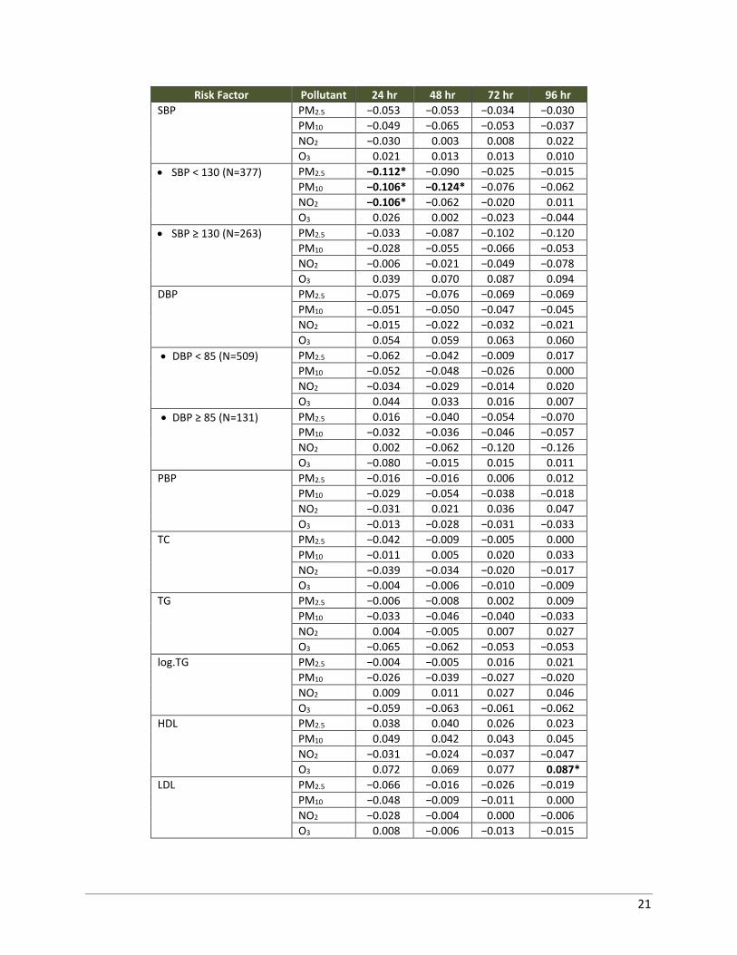
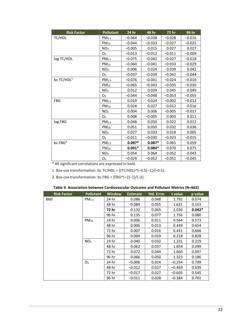
Correlation and regression analyses showed that the continuous types of MetS risk factors, such as waist

circumference, HDL, and fast blooding glucose, were associated with pollutant measurements. Table 8 and Table 9

show detailed results of the correlation and regression analyses, respectively. Waist circumference, in particular

for females, is a significant factor showing strong relationships with most of the pollutants: positive correlation

with PM2.5 and NO2 for all exposure periods (p-values < 0.005), and negative correlation with all O3 measurement

(p-values < 0.050). The relationship between waist circumference and PM2.5 may be due to a strong correlation

observed between BMI and waist circumference with a high correlation coefficient of 0.856 (0.870 for females and

0.893 for males). The 72-hr PM2.5 concentration was found to be positively associated with BMI (β1 = 0.132, p-value

= 0.042).

A significant relationship was found between 96-hr averaged O3 and HDL, showing positive correlation with β1 =

0.136 (p-value = 0.028). The increase in 24- and 48-hr PM2.5 and PM10 were significantly associated with an

increase in the box-cox transformed FBG scale (p-values < 0.05) but not for the original scale of FBG. The

transformation of FBG was suitable to find linear relationships with air pollution measurement.

Table 8. Correlation Analysis (N=662)

Risk Factor Pollutant 24 hr 48 hr 72 hr 96 hr

BMI PM2.5 0.070 0.064 0.080* 0.069

PM10 0.022 0.018 0.017 0.009

NO2 0.048 0.065 0.065 0.052

O3 −0.010 −0.018 −0.024 −0.015

Waist (overall) PM2.5 0.113* 0.121* 0.134* 0.129*

PM10 0.031 0.043 0.045 0.045

NO2 0.126* 0.149* 0.158* 0.142*

O3 −0.098* −0.112* −0.117* −0.107*

• Waist (female, N=559) PM2.5 0.148* 0.161* 0.179* 0.171*

PM10 0.050 0.068 0.076 0.077

NO2 0.126* 0.157* 0.164* 0.141*

O3 −0.100* −0.118* −0.123* −0.108*

• Waist (male, N=103) PM2.5 −0.036 −0.060 −0.084 −0.063

PM10 −0.056 −0.086 −0.127 −0.124

NO2 0.150 0.126 0.130 0.155

O3 −0.118 −0.109 −0.112 −0.128

21


SBP PM2.5 −0.053 −0.053 −0.034 −0.030

PM10 −0.049 −0.065 −0.053 −0.037

NO2 −0.030 0.003 0.008 0.022

O3 0.021 0.013 0.013 0.010

• SBP < 130 (N=377) PM2.5 −0.112* −0.090 −0.025 −0.015

PM10 −0.106* −0.124* −0.076 −0.062

NO2 −0.106* −0.062 −0.020 0.011

O3 0.026 0.002 −0.023 −0.044

• SBP ≥ 130 (N=263) PM2.5 −0.033 −0.087 −0.102 −0.120

PM10 −0.028 −0.055 −0.066 −0.053

NO2 −0.006 −0.021 −0.049 −0.078

O3 0.039 0.070 0.087 0.094

DBP PM2.5 −0.075 −0.076 −0.069 −0.069

PM10 −0.051 −0.050 −0.047 −0.045

NO2 −0.015 −0.022 −0.032 −0.021

O3 0.054 0.059 0.063 0.060

• DBP < 85 (N=509) PM2.5 −0.062 −0.042 −0.009 0.017

PM10 −0.052 −0.048 −0.026 0.000

NO2 −0.034 −0.029 −0.014 0.020

O3 0.044 0.033 0.016 0.007

• DBP ≥ 85 (N=131) PM2.5 0.016 −0.040 −0.054 −0.070

PM10 −0.032 −0.036 −0.046 −0.057

NO2 0.002 −0.062 −0.120 −0.126

O3 −0.080 −0.015 0.015 0.011

PBP PM2.5 −0.016 −0.016 0.006 0.012

PM10 −0.029 −0.054 −0.038 −0.018

NO2 −0.031 0.021 0.036 0.047

O3 −0.013 −0.028 −0.031 −0.033

TC PM2.5 −0.042 −0.009 −0.005 0.000

PM10 −0.011 0.005 0.020 0.033

NO2 −0.039 −0.034 −0.020 −0.017

O3 −0.004 −0.006 −0.010 −0.009

TG PM2.5 −0.006 −0.008 0.002 0.009

PM10 −0.033 −0.046 −0.040 −0.033

NO2 0.004 −0.005 0.007 0.027

O3 −0.065 −0.062 −0.053 −0.053

log.TG PM2.5 −0.004 −0.005 0.016 0.021

PM10 −0.026 −0.039 −0.027 −0.020

NO2 0.009 0.011 0.027 0.046

O3 −0.059 −0.063 −0.061 −0.062

HDL PM2.5 0.038 0.040 0.026 0.023

PM10 0.049 0.042 0.043 0.045

NO2 −0.031 −0.024 −0.037 −0.047

O3 0.072 0.069 0.077 0.087*

LDL PM2.5 −0.066 −0.016 −0.026 −0.019

PM10 −0.048 −0.009 −0.011 0.000

NO2 −0.028 −0.004 0.000 −0.006

O3 0.008 −0.006 −0.013 −0.015

22


TC/HDL PM2.5 −0.064 −0.038 −0.028 −0.016

PM10 −0.044 −0.033 −0.027 −0.025

NO2 −0.005 0.015 0.027 0.027

O3 −0.013 −0.012 −0.011 −0.009

log.TC/HDL PM2.5 −0.075 −0.042 −0.027 −0.018

PM10 −0.060 −0.041 −0.033 −0.029

NO2 0.006 0.024 0.039 0.042

O3 −0.037 −0.039 −0.042 −0.044

bc.TC/HDL1 PM2.5 −0.076 −0.041 −0.024 −0.016

PM10 −0.065 −0.043 −0.035 −0.030

NO2 0.012 0.029 0.045 0.049

O3 −0.044 −0.048 −0.053 −0.055

FBG PM2.5 0.019 0.024 −0.002 −0.012

PM10 0.024 0.027 0.012 0.016

NO2 0.004 0.006 −0.005 −0.017

O3 0.008 −0.005 0.003 0.011

log.FBG PM2.5 0.048 0.050 0.022 0.012

PM10 0.051 0.050 0.032 0.036

NO2 0.027 0.033 0.018 0.005

O3 −0.011 −0.030 −0.023 −0.015

bc.FBG2 PM2.5 0.087* 0.087* 0.065 0.059

PM10 0.091* 0.084* 0.070 0.075

NO2 0.054 0.064 0.052 0.043

O3 −0.029 −0.052 −0.051 −0.045

* All significant correlations are expressed in bold.

1. Box-cox transformation: bc.TC/HDL = [(TC/HDL)^(−0.5)−1]/(−0.5).

2. Box-cox transformation: bc.FBG = [FBG^(−2)−1]/(−2).

Table 9. Association between Cardiovascular Outcome and Pollutant Metrics (N=662)

Risk Factor Pollutant Window Estimate Std. Error t value p value

BMI PM2.5 24 hr 0.086 0.048 1.792 0.074

48 hr 0.089 0.055 1.631 0.103

72 hr 0.132 0.065 2.036 0.042*

96 hr 0.135 0.077 1.756 0.080

PM10 24 hr 0.006 0.011 0.564 0.573

48 hr 0.006 0.013 0.449 0.654

72 hr 0.007 0.016 0.431 0.666

96 hr 0.004 0.019 0.218 0.828

NO2 24 hr 0.040 0.032 1.231 0.219

48 hr 0.062 0.037 1.654 0.099

72 hr 0.072 0.044 1.660 0.097

96 hr 0.066 0.050 1.323 0.186

O3 24 hr −0.006 0.024 −0.254 0.799

48 hr −0.012 0.027 −0.469 0.639

72 hr −0.017 0.027 −0.605 0.545

96 hr −0.011 0.028 −0.384 0.701

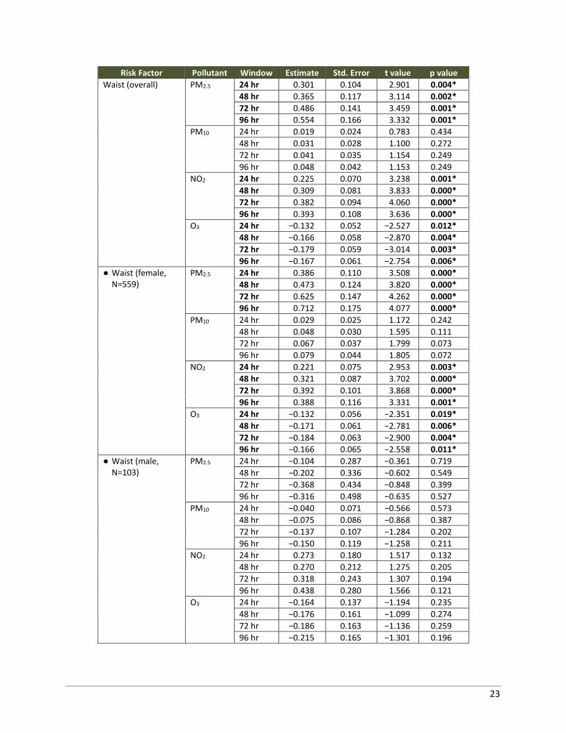
23


Waist (overall) PM2.5 24 hr 0.301 0.104 2.901 0.004*

48 hr 0.365 0.117 3.114 0.002*

72 hr 0.486 0.141 3.459 0.001*

96 hr 0.554 0.166 3.332 0.001*

PM10 24 hr 0.019 0.024 0.783 0.434

48 hr 0.031 0.028 1.100 0.272

72 hr 0.041 0.035 1.154 0.249

96 hr 0.048 0.042 1.153 0.249

NO2 24 hr 0.225 0.070 3.238 0.001*

48 hr 0.309 0.081 3.833 0.000*

72 hr 0.382 0.094 4.060 0.000*

96 hr 0.393 0.108 3.636 0.000*

O3 24 hr −0.132 0.052 −2.527 0.012*

48 hr −0.166 0.058 −2.870 0.004*

72 hr −0.179 0.059 −3.014 0.003*

96 hr −0.167 0.061 −2.754 0.006*

● Waist (female, N=559)

PM2.5 24 hr 0.386 0.110 3.508 0.000*

48 hr 0.473 0.124 3.820 0.000*

72 hr 0.625 0.147 4.262 0.000*

96 hr 0.712 0.175 4.077 0.000*

PM10 24 hr 0.029 0.025 1.172 0.242

48 hr 0.048 0.030 1.595 0.111

72 hr 0.067 0.037 1.799 0.073

96 hr 0.079 0.044 1.805 0.072

NO2 24 hr 0.221 0.075 2.953 0.003*

48 hr 0.321 0.087 3.702 0.000*

72 hr 0.392 0.101 3.868 0.000*

96 hr 0.388 0.116 3.331 0.001*

O3 24 hr −0.132 0.056 −2.351 0.019*

48 hr −0.171 0.061 −2.781 0.006*

72 hr −0.184 0.063 −2.900 0.004*

96 hr −0.166 0.065 −2.558 0.011*

● Waist (male, N=103)

PM2.5 24 hr −0.104 0.287 −0.361 0.719

48 hr −0.202 0.336 −0.602 0.549

72 hr −0.368 0.434 −0.848 0.399

96 hr −0.316 0.498 −0.635 0.527

PM10 24 hr −0.040 0.071 −0.566 0.573

48 hr −0.075 0.086 −0.868 0.387

72 hr −0.137 0.107 −1.284 0.202

96 hr −0.150 0.119 −1.258 0.211

NO2 24 hr 0.273 0.180 1.517 0.132

48 hr 0.270 0.212 1.275 0.205

72 hr 0.318 0.243 1.307 0.194

96 hr 0.438 0.280 1.566 0.121

O3 24 hr −0.164 0.137 −1.194 0.235

48 hr −0.176 0.161 −1.099 0.274

72 hr −0.186 0.163 −1.136 0.259

96 hr −0.215 0.165 −1.301 0.196

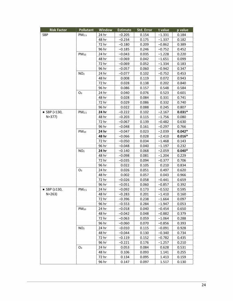
24


SBP PM2.5 24 hr −0.205 0.154 −1.331 0.184

48 hr −0.234 0.175 −1.337 0.182

72 hr −0.180 0.209 −0.862 0.389

96 hr −0.185 0.246 −0.752 0.452

PM10 24 hr −0.043 0.035 −1.228 0.220

48 hr −0.069 0.042 −1.651 0.099

72 hr −0.069 0.052 −1.334 0.183

96 hr −0.057 0.060 −0.942 0.347

NO2 24 hr −0.077 0.102 −0.752 0.453

48 hr 0.008 0.119 0.072 0.943

72 hr 0.028 0.138 0.202 0.840

96 hr 0.086 0.157 0.548 0.584

O3 24 hr 0.040 0.076 0.523 0.601

48 hr 0.028 0.084 0.331 0.741

72 hr 0.029 0.086 0.332 0.740

96 hr 0.022 0.088 0.245 0.807

● SBP (<130, N=377)

PM2.5 24 hr −0.222 0.102 −2.167 0.031*

48 hr −0.203 0.115 −1.756 0.080

72 hr −0.067 0.139 −0.482 0.630

96 hr −0.048 0.161 −0.297 0.766

PM10 24 hr −0.047 0.023 −2.039 0.042*

48 hr −0.066 0.028 −2.410 0.016*

72 hr −0.050 0.034 −1.468 0.143

96 hr −0.048 0.040 −1.197 0.232

NO2 24 hr −0.140 0.068 −2.059 0.040*

48 hr −0.098 0.081 −1.204 0.229

72 hr −0.035 0.094 −0.377 0.706

96 hr 0.022 0.105 0.210 0.834

O3 24 hr 0.026 0.051 0.497 0.620

48 hr 0.002 0.057 0.043 0.966

72 hr −0.026 0.058 −0.441 0.659

96 hr −0.051 0.060 −0.857 0.392

● SBP (≥130, N=263)

PM2.5 24 hr −0.092 0.173 −0.532 0.595

48 hr −0.283 0.201 −1.410 0.160

72 hr −0.396 0.238 −1.664 0.097

96 hr −0.553 0.284 −1.947 0.053

PM10 24 hr −0.018 0.040 −0.454 0.650

48 hr −0.042 0.048 −0.882 0.379

72 hr −0.063 0.059 −1.064 0.288

96 hr −0.060 0.070 −0.856 0.393

NO2 24 hr −0.010 0.115 −0.091 0.928

48 hr −0.044 0.130 −0.340 0.734

72 hr −0.119 0.152 −0.782 0.435

96 hr −0.221 0.176 −1.257 0.210

O3 24 hr 0.053 0.084 0.628 0.531

48 hr 0.106 0.093 1.141 0.255

72 hr 0.134 0.095 1.413 0.159

96 hr 0.147 0.097 1.517 0.130

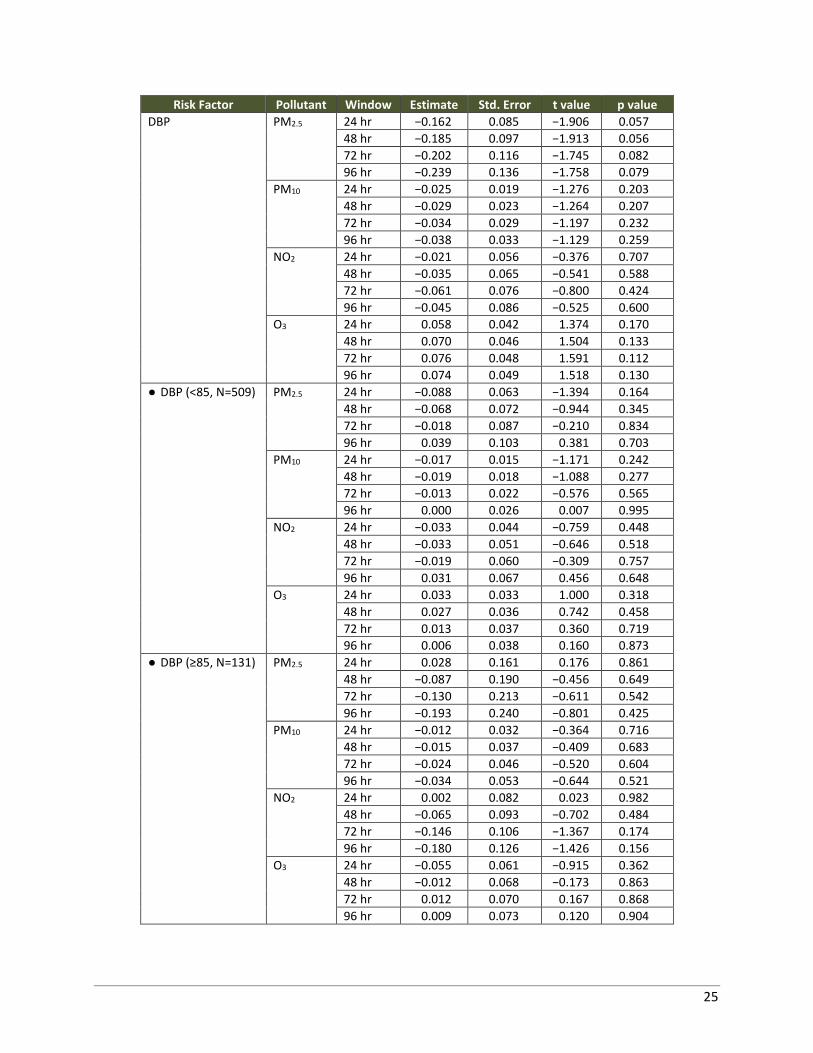
25


DBP PM2.5 24 hr −0.162 0.085 −1.906 0.057

48 hr −0.185 0.097 −1.913 0.056

72 hr −0.202 0.116 −1.745 0.082

96 hr −0.239 0.136 −1.758 0.079

PM10 24 hr −0.025 0.019 −1.276 0.203

48 hr −0.029 0.023 −1.264 0.207

72 hr −0.034 0.029 −1.197 0.232

96 hr −0.038 0.033 −1.129 0.259

NO2 24 hr −0.021 0.056 −0.376 0.707

48 hr −0.035 0.065 −0.541 0.588

72 hr −0.061 0.076 −0.800 0.424

96 hr −0.045 0.086 −0.525 0.600

O3 24 hr 0.058 0.042 1.374 0.170

48 hr 0.070 0.046 1.504 0.133

72 hr 0.076 0.048 1.591 0.112

96 hr 0.074 0.049 1.518 0.130

● DBP (<85, N=509) PM2.5 24 hr −0.088 0.063 −1.394 0.164

48 hr −0.068 0.072 −0.944 0.345

72 hr −0.018 0.087 −0.210 0.834

96 hr 0.039 0.103 0.381 0.703

PM10 24 hr −0.017 0.015 −1.171 0.242

48 hr −0.019 0.018 −1.088 0.277

72 hr −0.013 0.022 −0.576 0.565

96 hr 0.000 0.026 0.007 0.995

NO2 24 hr −0.033 0.044 −0.759 0.448

48 hr −0.033 0.051 −0.646 0.518

72 hr −0.019 0.060 −0.309 0.757

96 hr 0.031 0.067 0.456 0.648

O3 24 hr 0.033 0.033 1.000 0.318

48 hr 0.027 0.036 0.742 0.458

72 hr 0.013 0.037 0.360 0.719

96 hr 0.006 0.038 0.160 0.873

● DBP (≥85, N=131) PM2.5 24 hr 0.028 0.161 0.176 0.861

48 hr −0.087 0.190 −0.456 0.649

72 hr −0.130 0.213 −0.611 0.542

96 hr −0.193 0.240 −0.801 0.425

PM10 24 hr −0.012 0.032 −0.364 0.716

48 hr −0.015 0.037 −0.409 0.683

72 hr −0.024 0.046 −0.520 0.604

96 hr −0.034 0.053 −0.644 0.521

NO2 24 hr 0.002 0.082 0.023 0.982

48 hr −0.065 0.093 −0.702 0.484

72 hr −0.146 0.106 −1.367 0.174

96 hr −0.180 0.126 −1.426 0.156

O3 24 hr −0.055 0.061 −0.915 0.362

48 hr −0.012 0.068 −0.173 0.863

72 hr 0.012 0.070 0.167 0.868

96 hr 0.009 0.073 0.120 0.904

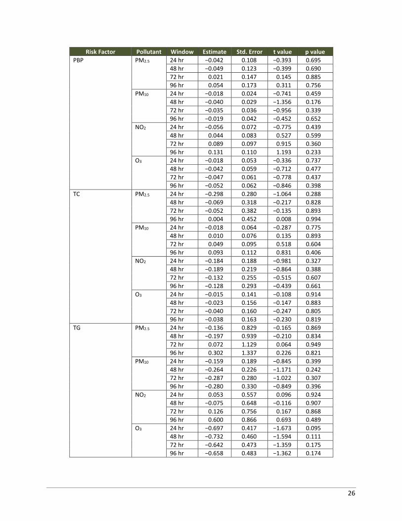
26


PBP PM2.5 24 hr −0.042 0.108 −0.393 0.695

48 hr −0.049 0.123 −0.399 0.690

72 hr 0.021 0.147 0.145 0.885

96 hr 0.054 0.173 0.311 0.756

PM10 24 hr −0.018 0.024 −0.741 0.459

48 hr −0.040 0.029 −1.356 0.176

72 hr −0.035 0.036 −0.956 0.339

96 hr −0.019 0.042 −0.452 0.652

NO2 24 hr −0.056 0.072 −0.775 0.439

48 hr 0.044 0.083 0.527 0.599

72 hr 0.089 0.097 0.915 0.360

96 hr 0.131 0.110 1.193 0.233

O3 24 hr −0.018 0.053 −0.336 0.737

48 hr −0.042 0.059 −0.712 0.477

72 hr −0.047 0.061 −0.778 0.437

96 hr −0.052 0.062 −0.846 0.398

TC PM2.5 24 hr −0.298 0.280 −1.064 0.288

48 hr −0.069 0.318 −0.217 0.828

72 hr −0.052 0.382 −0.135 0.893

96 hr 0.004 0.452 0.008 0.994

PM10 24 hr −0.018 0.064 −0.287 0.775

48 hr 0.010 0.076 0.135 0.893

72 hr 0.049 0.095 0.518 0.604

96 hr 0.093 0.112 0.831 0.406

NO2 24 hr −0.184 0.188 −0.981 0.327

48 hr −0.189 0.219 −0.864 0.388

72 hr −0.132 0.255 −0.515 0.607

96 hr −0.128 0.293 −0.439 0.661

O3 24 hr −0.015 0.141 −0.108 0.914

48 hr −0.023 0.156 −0.147 0.883

72 hr −0.040 0.160 −0.247 0.805

96 hr −0.038 0.163 −0.230 0.819

TG PM2.5 24 hr −0.136 0.829 −0.165 0.869

48 hr −0.197 0.939 −0.210 0.834

72 hr 0.072 1.129 0.064 0.949

96 hr 0.302 1.337 0.226 0.821

PM10 24 hr −0.159 0.189 −0.845 0.399

48 hr −0.264 0.226 −1.171 0.242

72 hr −0.287 0.280 −1.022 0.307

96 hr −0.280 0.330 −0.849 0.396

NO2 24 hr 0.053 0.557 0.096 0.924

48 hr −0.075 0.648 −0.116 0.907

72 hr 0.126 0.756 0.167 0.868

96 hr 0.600 0.866 0.693 0.489

O3 24 hr −0.697 0.417 −1.673 0.095

48 hr −0.732 0.460 −1.594 0.111

72 hr −0.642 0.473 −1.359 0.175

96 hr −0.658 0.483 −1.362 0.174

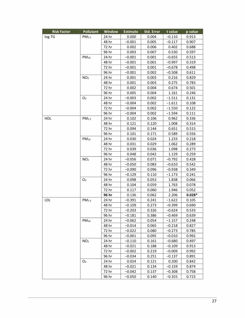
27


log.TG PM2.5 24 hr 0.000 0.004 −0.110 0.913

48 hr −0.001 0.005 −0.117 0.907

72 hr 0.002 0.006 0.402 0.688

96 hr 0.003 0.007 0.530 0.597

PM10 24 hr −0.001 0.001 −0.655 0.513

48 hr −0.001 0.001 −0.997 0.319

72 hr −0.001 0.001 −0.678 0.498

96 hr −0.001 0.002 −0.508 0.611

NO2 24 hr 0.001 0.003 0.216 0.829

48 hr 0.001 0.003 0.275 0.783

72 hr 0.002 0.004 0.674 0.501

96 hr 0.005 0.004 1.161 0.246

O3 24 hr −0.003 0.002 −1.511 0.131

48 hr −0.004 0.002 −1.611 0.108

72 hr −0.004 0.002 −1.550 0.122

96 hr −0.004 0.002 −1.594 0.111

HDL PM2.5 24 hr 0.102 0.106 0.962 0.336

48 hr 0.121 0.120 1.008 0.314

72 hr 0.094 0.144 0.651 0.515

96 hr 0.101 0.171 0.589 0.556

PM10 24 hr 0.030 0.024 1.233 0.218

48 hr 0.031 0.029 1.062 0.289

72 hr 0.039 0.036 1.098 0.273

96 hr 0.048 0.042 1.129 0.259

NO2 24 hr −0.056 0.071 −0.792 0.428

48 hr −0.050 0.083 −0.610 0.542

72 hr −0.090 0.096 −0.938 0.349

96 hr −0.129 0.110 −1.173 0.241

O3 24 hr 0.098 0.053 1.838 0.066

48 hr 0.104 0.059 1.763 0.078

72 hr 0.117 0.060 1.946 0.052

96 hr 0.136 0.062 2.206 0.028*

LDL PM2.5 24 hr −0.391 0.241 −1.622 0.105

48 hr −0.109 0.273 −0.399 0.690

72 hr −0.203 0.326 −0.624 0.533

96 hr −0.181 0.386 −0.469 0.639

PM10 24 hr −0.062 0.054 −1.157 0.248

48 hr −0.014 0.065 −0.218 0.827

72 hr −0.022 0.080 −0.273 0.785

96 hr −0.001 0.095 −0.010 0.992

NO2 24 hr −0.110 0.161 −0.680 0.497

48 hr −0.021 0.188 −0.109 0.913

72 hr −0.002 0.219 −0.009 0.992

96 hr −0.034 0.251 −0.137 0.891

O3 24 hr 0.024 0.121 0.200 0.842

48 hr −0.021 0.134 −0.159 0.874

72 hr −0.042 0.137 −0.308 0.758

96 hr −0.050 0.140 −0.355 0.723

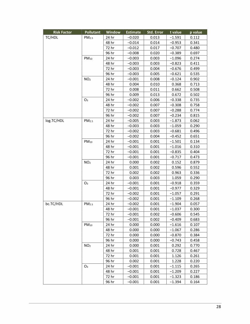
28


TC/HDL PM2.5 24 hr −0.020 0.013 −1.591 0.112

48 hr −0.014 0.014 −0.953 0.341

72 hr −0.012 0.017 −0.707 0.480

96 hr −0.008 0.020 −0.389 0.697

PM10 24 hr −0.003 0.003 −1.096 0.274

48 hr −0.003 0.003 −0.823 0.411

72 hr −0.003 0.004 −0.676 0.499

96 hr −0.003 0.005 −0.621 0.535

NO2 24 hr −0.001 0.008 −0.124 0.902

48 hr 0.004 0.010 0.368 0.713

72 hr 0.008 0.011 0.662 0.508

96 hr 0.009 0.013 0.672 0.502

O3 24 hr −0.002 0.006 −0.338 0.735

48 hr −0.002 0.007 −0.308 0.758

72 hr −0.002 0.007 −0.288 0.774

96 hr −0.002 0.007 −0.234 0.815

log.TC/HDL PM2.5 24 hr −0.005 0.003 −1.873 0.062

48 hr −0.003 0.003 −1.059 0.290

72 hr −0.002 0.003 −0.681 0.496

96 hr −0.002 0.004 −0.452 0.651

PM10 24 hr −0.001 0.001 −1.501 0.134

48 hr −0.001 0.001 −1.016 0.310

72 hr −0.001 0.001 −0.835 0.404

96 hr −0.001 0.001 −0.717 0.473

NO2 24 hr 0.000 0.002 0.152 0.879

48 hr 0.001 0.002 0.596 0.552

72 hr 0.002 0.002 0.963 0.336

96 hr 0.003 0.003 1.059 0.290

O3 24 hr −0.001 0.001 −0.918 0.359

48 hr −0.001 0.001 −0.977 0.329

72 hr −0.002 0.001 −1.057 0.291

96 hr −0.002 0.001 −1.109 0.268

bc.TC/HDL PM2.5 24 hr −0.002 0.001 −1.904 0.057

48 hr −0.001 0.001 −1.037 0.300

72 hr −0.001 0.002 −0.606 0.545

96 hr −0.001 0.002 −0.409 0.683

PM10 24 hr 0.000 0.000 −1.616 0.107

48 hr 0.000 0.000 −1.067 0.286

72 hr 0.000 0.000 −0.870 0.384

96 hr 0.000 0.000 −0.743 0.458

NO2 24 hr 0.000 0.001 0.292 0.770

48 hr 0.001 0.001 0.728 0.467

72 hr 0.001 0.001 1.126 0.261

96 hr 0.002 0.001 1.228 0.220

O3 24 hr −0.001 0.001 −1.115 0.265

48 hr −0.001 0.001 −1.209 0.227

72 hr −0.001 0.001 −1.323 0.186

96 hr −0.001 0.001 −1.394 0.164

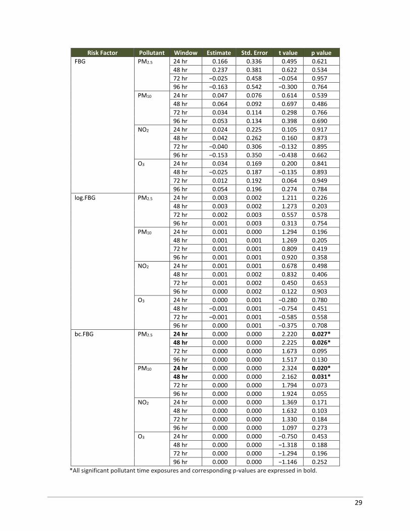
29


FBG PM2.5 24 hr 0.166 0.336 0.495 0.621

48 hr 0.237 0.381 0.622 0.534

72 hr −0.025 0.458 −0.054 0.957

96 hr −0.163 0.542 −0.300 0.764

PM10 24 hr 0.047 0.076 0.614 0.539

48 hr 0.064 0.092 0.697 0.486

72 hr 0.034 0.114 0.298 0.766

96 hr 0.053 0.134 0.398 0.690

NO2 24 hr 0.024 0.225 0.105 0.917

48 hr 0.042 0.262 0.160 0.873

72 hr −0.040 0.306 −0.132 0.895

96 hr −0.153 0.350 −0.438 0.662

O3 24 hr 0.034 0.169 0.200 0.841

48 hr −0.025 0.187 −0.135 0.893

72 hr 0.012 0.192 0.064 0.949

96 hr 0.054 0.196 0.274 0.784

log.FBG PM2.5 24 hr 0.003 0.002 1.211 0.226

48 hr 0.003 0.002 1.273 0.203

72 hr 0.002 0.003 0.557 0.578

96 hr 0.001 0.003 0.313 0.754

PM10 24 hr 0.001 0.000 1.294 0.196

48 hr 0.001 0.001 1.269 0.205

72 hr 0.001 0.001 0.809 0.419

96 hr 0.001 0.001 0.920 0.358

NO2 24 hr 0.001 0.001 0.678 0.498

48 hr 0.001 0.002 0.832 0.406

72 hr 0.001 0.002 0.450 0.653

96 hr 0.000 0.002 0.122 0.903

O3 24 hr 0.000 0.001 −0.280 0.780

48 hr −0.001 0.001 −0.754 0.451

72 hr −0.001 0.001 −0.585 0.558

96 hr 0.000 0.001 −0.375 0.708

bc.FBG PM2.5 24 hr 0.000 0.000 2.220 0.027*

48 hr 0.000 0.000 2.225 0.026*

72 hr 0.000 0.000 1.673 0.095

96 hr 0.000 0.000 1.517 0.130

PM10 24 hr 0.000 0.000 2.324 0.020*

48 hr 0.000 0.000 2.162 0.031*

72 hr 0.000 0.000 1.794 0.073

96 hr 0.000 0.000 1.924 0.055

NO2 24 hr 0.000 0.000 1.369 0.171

48 hr 0.000 0.000 1.632 0.103

72 hr 0.000 0.000 1.330 0.184

96 hr 0.000 0.000 1.097 0.273

O3 24 hr 0.000 0.000 −0.750 0.453

48 hr 0.000 0.000 −1.318 0.188

72 hr 0.000 0.000 −1.294 0.196

96 hr 0.000 0.000 −1.146 0.252


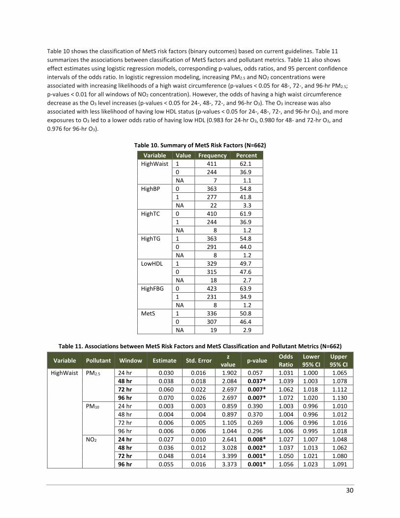
30

Table 10 shows the classification of MetS risk factors (binary outcomes) based on current guidelines. Table 11

summarizes the associations between classification of MetS factors and pollutant metrics. Table 11 also shows

effect estimates using logistic regression models, corresponding p-values, odds ratios, and 95 percent confidence

intervals of the odds ratio. In logistic regression modeling, increasing PM2.5 and NO2 concentrations were

associated with increasing likelihoods of a high waist circumference (p-values < 0.05 for 48-, 72-, and 96-hr PM2.5;

p-values < 0.01 for all windows of NO2 concentration). However, the odds of having a high waist circumference

decrease as the O3 level increases (p-values < 0.05 for 24-, 48-, 72-, and 96-hr O3). The O3 increase was also

associated with less likelihood of having low HDL status (p-values < 0.05 for 24-, 48-, 72-, and 96-hr O3), and more

exposures to O3 led to a lower odds ratio of having low HDL (0.983 for 24-hr O3, 0.980 for 48- and 72-hr O3, and

0.976 for 96-hr O3).

Table 10. Summary of MetS Risk Factors (N=662)

Variable Value Frequency Percent

HighWaist 1 411 62.1

0 244 36.9

NA 7 1.1

HighBP 0 363 54.8

1 277 41.8

NA 22 3.3

HighTC 0 410 61.9

1 244 36.9

NA 8 1.2

HighTG 1 363 54.8

0 291 44.0

NA 8 1.2

LowHDL 1 329 49.7

0 315 47.6

NA 18 2.7

HighFBG 0 423 63.9

1 231 34.9

NA 8 1.2

MetS 1 336 50.8

0 307 46.4

NA 19 2.9

Table 11. Associations between MetS Risk Factors and MetS Classification and Pollutant Metrics (N=662)

Variable Pollutant Window Estimate Std. Error z

value p-value

Odds Ratio

Lower 95% CI

Upper 95% CI

HighWaist PM2.5 24 hr 0.030 0.016 1.902 0.057 1.031 1.000 1.065

48 hr 0.038 0.018 2.084 0.037* 1.039 1.003 1.078

72 hr 0.060 0.022 2.697 0.007* 1.062 1.018 1.112

96 hr 0.070 0.026 2.697 0.007* 1.072 1.020 1.130

PM10 24 hr 0.003 0.003 0.859 0.390 1.003 0.996 1.010

48 hr 0.004 0.004 0.897 0.370 1.004 0.996 1.012

72 hr 0.006 0.005 1.105 0.269 1.006 0.996 1.016

96 hr 0.006 0.006 1.044 0.296 1.006 0.995 1.018

NO2 24 hr 0.027 0.010 2.641 0.008* 1.027 1.007 1.048

48 hr 0.036 0.012 3.028 0.002* 1.037 1.013 1.062

72 hr 0.048 0.014 3.399 0.001* 1.050 1.021 1.080

96 hr 0.055 0.016 3.373 0.001* 1.056 1.023 1.091

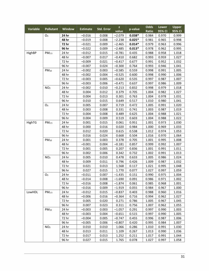
31


value p-value

Odds Ratio

Lower 95% CI

Upper 95% CI

O3 24 hr –0.016 0.008 –2.079 0.038* 0.984 0.970 0.999

48 hr –0.019 0.008 –2.238 0.025* 0.981 0.965 0.998

72 hr –0.021 0.009 –2.465 0.014* 0.979 0.963 0.996

96 hr –0.022 0.009 –2.485 0.013* 0.978 0.962 0.995

HighBP PM2.5 24 hr –0.012 0.015 –0.781 0.435 0.988 0.958 1.018

48 hr –0.007 0.017 –0.410 0.682 0.993 0.959 1.027

72 hr –0.009 0.021 –0.417 0.677 0.991 0.952 1.032

96 hr –0.007 0.024 –0.300 0.764 0.993 0.946 1.041

PM10 24 hr –0.002 0.003 –0.585 0.559 0.998 0.991 1.005

48 hr –0.002 0.004 –0.525 0.600 0.998 0.990 1.006

72 hr –0.003 0.005 –0.620 0.535 0.997 0.987 1.007

96 hr –0.003 0.006 –0.471 0.637 0.997 0.986 1.009

NO2 24 hr –0.002 0.010 –0.213 0.832 0.998 0.979 1.018

48 hr 0.004 0.012 0.379 0.705 1.004 0.982 1.027

72 hr 0.004 0.013 0.301 0.763 1.004 0.978 1.031

96 hr 0.010 0.015 0.649 0.517 1.010 0.980 1.041

O3 24 hr 0.005 0.007 0.719 0.472 1.005 0.991 1.020

48 hr 0.003 0.008 0.331 0.741 1.003 0.987 1.019

72 hr 0.004 0.008 0.489 0.625 1.004 0.988 1.021

96 hr 0.004 0.009 0.519 0.603 1.004 0.988 1.022

HighTG PM2.5 24 hr 0.001 0.015 0.061 0.951 1.001 0.973 1.030

48 hr 0.000 0.016 0.020 0.984 1.000 0.969 1.033

72 hr 0.012 0.020 0.615 0.538 1.012 0.974 1.053

96 hr 0.016 0.024 0.668 0.504 1.016 0.970 1.064

PM10 24 hr 0.001 0.003 0.378 0.705 1.001 0.995 1.008

48 hr –0.001 0.004 –0.181 0.857 0.999 0.992 1.007

72 hr 0.001 0.005 0.207 0.836 1.001 0.991 1.011

96 hr 0.002 0.006 0.342 0.732 1.002 0.991 1.013

NO2 24 hr 0.005 0.010 0.478 0.633 1.005 0.986 1.024

48 hr 0.009 0.011 0.796 0.426 1.009 0.987 1.032

72 hr 0.021 0.013 1.568 0.117 1.021 0.995 1.048

96 hr 0.027 0.015 1.770 0.077 1.027 0.997 1.059

O3 24 hr –0.011 0.007 –1.435 0.151 0.990 0.975 1.004

48 hr –0.014 0.008 –1.690 0.091 0.986 0.971 1.002

72 hr –0.016 0.008 –1.874 0.061 0.985 0.968 1.001

96 hr –0.016 0.009 –1.919 0.055 0.984 0.967 1.000

LowHDL PM2.5 24 hr –0.012 0.015 –0.837 0.403 0.988 0.960 1.016

48 hr –0.006 0.016 –0.364 0.716 0.994 0.962 1.027

72 hr 0.005 0.020 0.271 0.786 1.005 0.967 1.045

96 hr 0.007 0.023 0.311 0.756 1.007 0.962 1.055

PM10 24 hr –0.003 0.003 –1.057 0.291 0.997 0.990 1.003

48 hr –0.003 0.004 –0.651 0.515 0.997 0.990 1.005

72 hr –0.004 0.005 –0.747 0.455 0.996 0.987 1.006

96 hr –0.005 0.006 –0.807 0.420 0.995 0.984 1.007

NO2 24 hr 0.010 0.010 1.066 0.286 1.010 0.991 1.030

48 hr 0.013 0.011 1.109 0.267 1.013 0.990 1.036

72 hr 0.017 0.013 1.252 0.211 1.017 0.991 1.044

96 hr 0.027 0.015 1.765 0.078 1.027 0.997 1.058

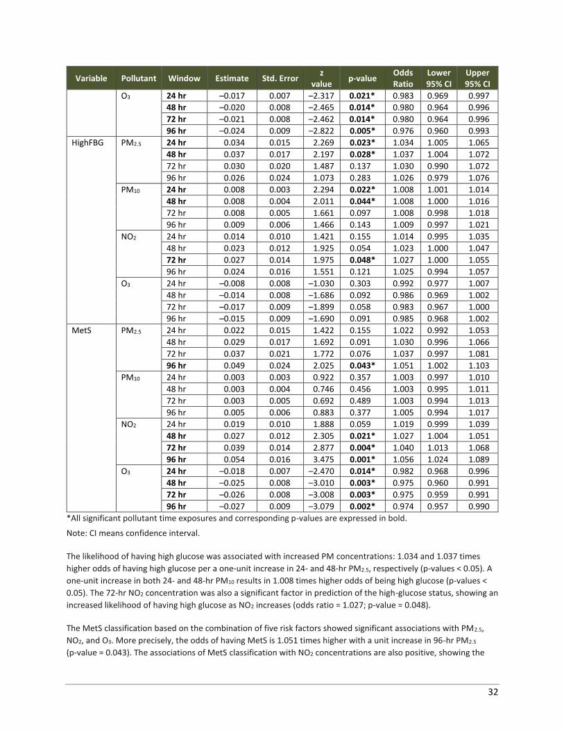
32


value p-value

Odds Ratio

Lower 95% CI

Upper 95% CI

O3 24 hr –0.017 0.007 –2.317 0.021* 0.983 0.969 0.997

48 hr –0.020 0.008 –2.465 0.014* 0.980 0.964 0.996

72 hr –0.021 0.008 –2.462 0.014* 0.980 0.964 0.996

96 hr –0.024 0.009 –2.822 0.005* 0.976 0.960 0.993

HighFBG PM2.5 24 hr 0.034 0.015 2.269 0.023* 1.034 1.005 1.065

48 hr 0.037 0.017 2.197 0.028* 1.037 1.004 1.072

72 hr 0.030 0.020 1.487 0.137 1.030 0.990 1.072

96 hr 0.026 0.024 1.073 0.283 1.026 0.979 1.076

PM10 24 hr 0.008 0.003 2.294 0.022* 1.008 1.001 1.014

48 hr 0.008 0.004 2.011 0.044* 1.008 1.000 1.016

72 hr 0.008 0.005 1.661 0.097 1.008 0.998 1.018

96 hr 0.009 0.006 1.466 0.143 1.009 0.997 1.021

NO2 24 hr 0.014 0.010 1.421 0.155 1.014 0.995 1.035

48 hr 0.023 0.012 1.925 0.054 1.023 1.000 1.047

72 hr 0.027 0.014 1.975 0.048* 1.027 1.000 1.055

96 hr 0.024 0.016 1.551 0.121 1.025 0.994 1.057

O3 24 hr –0.008 0.008 –1.030 0.303 0.992 0.977 1.007

48 hr –0.014 0.008 –1.686 0.092 0.986 0.969 1.002

72 hr –0.017 0.009 –1.899 0.058 0.983 0.967 1.000

96 hr –0.015 0.009 –1.690 0.091 0.985 0.968 1.002

MetS PM2.5 24 hr 0.022 0.015 1.422 0.155 1.022 0.992 1.053

48 hr 0.029 0.017 1.692 0.091 1.030 0.996 1.066

72 hr 0.037 0.021 1.772 0.076 1.037 0.997 1.081

96 hr 0.049 0.024 2.025 0.043* 1.051 1.002 1.103

PM10 24 hr 0.003 0.003 0.922 0.357 1.003 0.997 1.010

48 hr 0.003 0.004 0.746 0.456 1.003 0.995 1.011

72 hr 0.003 0.005 0.692 0.489 1.003 0.994 1.013

96 hr 0.005 0.006 0.883 0.377 1.005 0.994 1.017

NO2 24 hr 0.019 0.010 1.888 0.059 1.019 0.999 1.039

48 hr 0.027 0.012 2.305 0.021* 1.027 1.004 1.051

72 hr 0.039 0.014 2.877 0.004* 1.040 1.013 1.068

96 hr 0.054 0.016 3.475 0.001* 1.056 1.024 1.089

O3 24 hr –0.018 0.007 –2.470 0.014* 0.982 0.968 0.996

48 hr –0.025 0.008 –3.010 0.003* 0.975 0.960 0.991

72 hr –0.026 0.008 –3.008 0.003* 0.975 0.959 0.991

96 hr –0.027 0.009 –3.079 0.002* 0.974 0.957 0.990


Note: CI means confidence interval.

The likelihood of having high glucose was associated with increased PM concentrations: 1.034 and 1.037 times

higher odds of having high glucose per a one-unit increase in 24- and 48-hr PM2.5, respectively (p-values < 0.05). A

one-unit increase in both 24- and 48-hr PM10 results in 1.008 times higher odds of being high glucose (p-values <

0.05). The 72-hr NO2 concentration was also a significant factor in prediction of the high-glucose status, showing an

increased likelihood of having high glucose as NO2 increases (odds ratio = 1.027; p-value = 0.048).

The MetS classification based on the combination of five risk factors showed significant associations with PM2.5,

NO2, and O3. More precisely, the odds of having MetS is 1.051 times higher with a unit increase in 96-hr PM2.5

(p-value = 0.043). The associations of MetS classification with NO2 concentrations are also positive, showing the

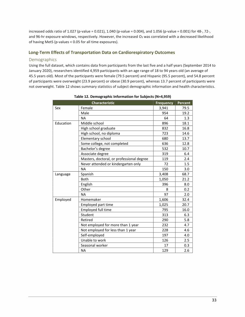
33

increased odds ratio of 1.027 (p-value = 0.021), 1.040 (p-value = 0.004), and 1.056 (p-value = 0.001) for 48-, 72-,

and 96-hr exposure windows, respectively. However, the increased O3 was correlated with a decreased likelihood

of having MetS (p-values < 0.05 for all time exposures).

Long-Term Effects of Transportation Data on Cardiorespiratory Outcomes

Demographics Using the full dataset, which contains data from participants from the last five and a half years (September 2014 to

January 2020), researchers identified 4,959 participants with an age range of 18 to 94 years old (an average of

45.5 years old). Most of the participants were female (79.5 percent) and Hispanic (95.5 percent), and 54.8 percent

of participants were overweight (23.9 percent) or obese (30.9 percent), whereas 13.7 percent of participants were

not overweight. Table 12 shows summary statistics of subject demographic information and health characteristics.

Table 12. Demographic Information for Subjects (N=4,959)


Sex

Female 3,941 79.5

Male 954 19.2

NA 64 1.3

Education

Middle school 896 18.1

High school graduate 832 16.8

High school, no diploma 723 14.6

Elementary school 680 13.7

Some college, not completed 636 12.8

Bachelor’s degree 532 10.7

Associate degree 319 6.4

Masters, doctoral, or professional degree 119 2.4

Never attended or kindergarten only 72 1.5

NA 150 3.0

Language

Spanish 3,408 68.7

Both 1,050 21.2

English 396 8.0

Other 8 0.2

NA 97 2.0

Employed

Homemaker 1,606 32.4

Employed part time 1,025 20.7

Employed full time 795 16.0

Student 313 6.3

Retired 290 5.8

Not employed for more than 1 year 232 4.7

Not employed for less than 1 year 228 4.6

Self-employed 197 4.0

Unable to work 126 2.5

Seasonal worker 17 0.3

NA 129 2.6

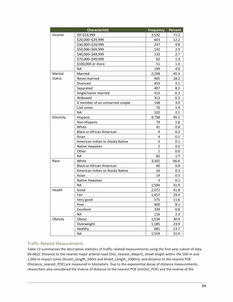
34


Income

$0–$19,999 3,532 71.2

$20,000–$29,999 603 12.2

$30,000–$39,999 237 4.8

$50,000–$69,999 142 2.9

$40,000–$49,999 133 2.7

$70,000–$99,999 62 1.3

$100,000 or more 51 1.0

NA 199 4.0

Marital status

Married 2,248 45.3

Never married 905 18.2

Divorced 453 9.1

Separated 407 8.2

Single/never married 313 6.3

Widowed 313 6.3

A member of an unmarried couple 148 3.0

Civil union 70 1.4

NA 102 2.1

Ethnicity

Hispanic 4,738 95.5

Non-Hispanic 79 1.6

White 41 0.8


Asian 4 0.1


Native Hawaiian 2 0.0

Other 1 0.0

NA 82 1.7

Race

White 3,302 66.6



Asian 14 0.3

Native Hawaiian 3 0.1

NA 1,584 31.9

Health

Good 2,072 41.8

Fair 1,457 29.4

Very good 575 11.6

Poor 400 8.1

Excellent 339 6.8

NA 116 2.3

Obesity

Obese 1,534 30.9

Overweight 1,185 23.9

Healthy 681 13.7

NA 1,559 31.4

Traffic-Related Measurements Table 13 summarizes the descriptive statistics of traffic-related measurements using the first-year subset of data

(N=662). Distance to the nearest major arterial road (Dist_nearest_Majart), street length within the 500-m and

1,000-m impact zones (Street_Length_500m and Street_Length_1000m), and distance to the nearest POE

(Distance_nearest_POE) are measured in kilometers. Due to the exponential decay of distance measurements,

researchers also considered the inverse of distance to the nearest POE (InvDist_POE) and the inverse of the

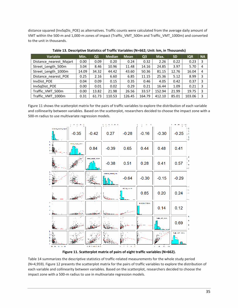
35

distance squared (InvSqDis_POE) as alternatives. Traffic counts were calculated from the average daily amount of

VMT within the 500-m and 1,000-m zones of impact (Traffic_VMT_500m and Traffic_VMT_1000m) and converted

to the unit in thousands.

Table 13. Descriptive Statistics of Traffic Variables (N=662; Unit: km, in Thousands)

Variable Min. Q1 Median Mean Q3 Max. SD IQR NA

Distance_nearest_Majart 0.00 0.09 0.20 0.24 0.32 2.26 0.22 0.23 3

Street_Length_500m 3.04 8.46 10.96 11.48 14.16 24.85 3.97 5.70 4

Street_Length_1000m 14.09 34.32 44.42 43.60 50.36 81.15 12.76 16.04 4

Distance_nearest_POE 0.25 2.16 6.60 6.85 11.15 25.36 5.12 8.99 3

InvDist_POE 0.04 0.09 0.15 0.35 0.46 4.05 0.42 0.37 3

InvSqDist_POE 0.00 0.01 0.02 0.29 0.21 16.44 1.09 0.21 3

Traffic_VMT_500m 0.00 13.82 21.98 26.56 33.57 152.94 21.99 19.75 3

Traffic_VMT_1000m 0.31 61.73 110.53 126.45 164.79 412.10 85.01 103.06 3

Figure 11 shows the scatterplot matrix for the pairs of traffic variables to explore the distribution of each variable

and collinearity between variables. Based on the scatterplot, researchers decided to choose the impact zone with a

500-m radius to use multivariate regression models.

Figure 11. Scatterplot matrix of pairs of eight traffic variables (N=662).

Table 14 summarizes the descriptive statistics of traffic-related measurements for the whole study period

(N=4,959). Figure 12 presents the scatterplot matrix for the pairs of traffic variables to explore the distribution of

each variable and collinearity between variables. Based on the scatterplot, researchers decided to choose the

impact zone with a 500-m radius to use in multivariate regression models.

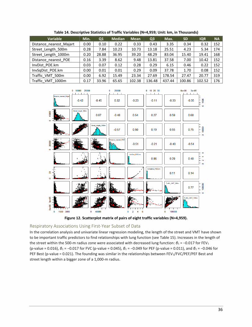
36

Table 14. Descriptive Statistics of Traffic Variables (N=4,959; Unit: km, in Thousands)

Variable Min. Q1 Median Mean Q3 Max. SD IQR NA

Distance_nearest_Majart 0.00 0.10 0.22 0.33 0.43 3.35 0.34 0.32 152

Street_Length_500m 0.28 7.84 10.23 10.73 13.18 25.51 4.23 5.34 174

Street_Length_1000m 0.20 28.88 36.95 39.20 48.29 83.04 15.40 19.41 168

Distance_nearest_POE 0.16 3.39 8.62 9.48 13.81 37.58 7.00 10.42 152

InvDist_POE.km 0.03 0.07 0.12 0.28 0.29 6.15 0.46 0.22 152

InvSqDist_POE.km 0.00 0.01 0.01 0.29 0.09 37.78 1.70 0.08 152

Traffic_VMT_500m 0.00 6.92 15.49 23.34 27.69 178.54 27.47 20.77 319

Traffic_VMT_1000m 0.17 33.96 65.65 102.38 136.48 437.44 100.86 102.52 176

Figure 12. Scatterplot matrix of pairs of eight traffic variables (N=4,959).

Respiratory Associations Using First-Year Subset of Data In the correlation analysis and univariate linear regression modeling, the length of the street and VMT have shown

to be important traffic predictors to find relationships with lung function (see Table 15). Increases in the length of

the street within the 500-m radius zone were associated with decreased lung function: β1 = −0.017 for FEV1

(p-value = 0.016), β1 = −0.017 for FVC (p-value = 0.045), β1 = −0.049 for PEF (p-value = 0.011), and β1 = −0.046 for

PEF Best (p-value = 0.021). The founding was similar in the relationships between FEV1/FVC/PEF/PEF Best and

street length within a bigger zone of a 1,000-m radius.

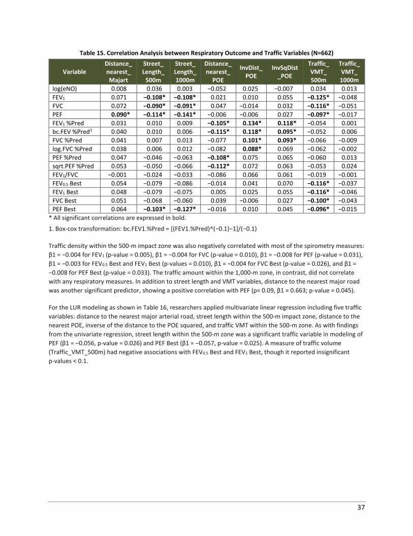
37

Table 15. Correlation Analysis between Respiratory Outcome and Traffic Variables (N=662)

Variable Distance_ nearest_ Majart

Street_ Length_

500m

Street_ Length_ 1000m

Distance_ nearest_

POE

InvDist_ POE

InvSqDist _POE

Traffic_ VMT_ 500m

Traffic_ VMT_ 1000m

log(eNO) 0.008 0.036 0.003 −0.052 0.025 −0.007 0.034 0.013

FEV1 0.071 −0.108* −0.108* 0.021 0.010 0.055 −0.125* −0.048

FVC 0.072 −0.090* −0.091* 0.047 −0.014 0.032 −0.116* −0.051

PEF 0.090* −0.114* −0.141* −0.006 −0.006 0.027 −0.097* −0.017

FEV1 %Pred 0.031 0.010 0.009 −0.105* 0.134* 0.118* −0.054 0.001

bc.FEV %Pred1 0.040 0.010 0.006 −0.115* 0.118* 0.095* −0.052 0.006

FVC %Pred 0.041 0.007 0.013 −0.077 0.101* 0.093* −0.066 −0.009

log.FVC %Pred 0.038 0.006 0.012 −0.082 0.088* 0.069 −0.062 −0.002

PEF %Pred 0.047 −0.046 −0.063 −0.108* 0.075 0.065 −0.060 0.013

sqrt.PEF %Pred 0.053 −0.050 −0.066 −0.112* 0.072 0.063 −0.053 0.024

FEV1/FVC −0.001 −0.024 −0.033 −0.086 0.066 0.061 −0.019 −0.001

FEV0.5 Best 0.054 −0.079 −0.086 −0.014 0.041 0.070 −0.116* −0.037

FEV1 Best 0.048 −0.079 −0.075 0.005 0.025 0.055 −0.116* −0.046

FVC Best 0.051 −0.068 −0.060 0.039 −0.006 0.027 −0.100* −0.043

PEF Best 0.064 −0.103* −0.127* −0.016 0.010 0.045 −0.096* −0.015


1. Box-cox transformation: bc.FEV1.%Pred = [(FEV1.%Pred)^(−0.1)−1]/(−0.1)

Traffic density within the 500-m impact zone was also negatively correlated with most of the spirometry measures:

β1 = −0.004 for FEV1 (p-value = 0.005), β1 = −0.004 for FVC (p-value = 0.010), β1 = −0.008 for PEF (p-value = 0.031),

β1 = −0.003 for FEV0.5 Best and FEV1 Best (p-values = 0.010), β1 = −0.004 for FVC Best (p-value = 0.026), and β1 =

−0.008 for PEF Best (p-value = 0.033). The traffic amount within the 1,000-m zone, in contrast, did not correlate

with any respiratory measures. In addition to street length and VMT variables, distance to the nearest major road

was another significant predictor, showing a positive correlation with PEF (ρ= 0.09, β1 = 0.663; p-value = 0.045).

For the LUR modeling as shown in Table 16, researchers applied multivariate linear regression including five traffic

variables: distance to the nearest major arterial road, street length within the 500-m impact zone, distance to the

nearest POE, inverse of the distance to the POE squared, and traffic VMT within the 500-m zone. As with findings

from the univariate regression, street length within the 500-m zone was a significant traffic variable in modeling of

PEF (β1 = −0.056, p-value = 0.026) and PEF Best (β1 = −0.057, p-value = 0.025). A measure of traffic volume

(Traffic_VMT_500m) had negative associations with FEV0.5 Best and FEV1 Best, though it reported insignificant

p-values < 0.1.

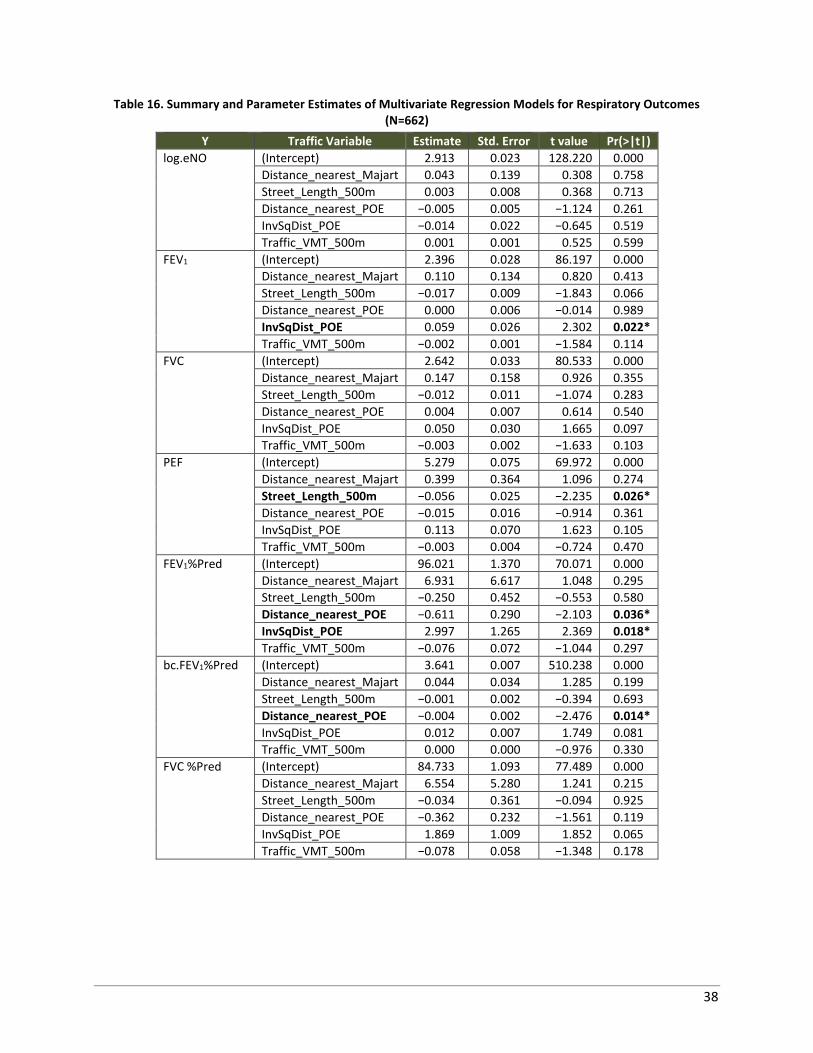
38

Table 16. Summary and Parameter Estimates of Multivariate Regression Models for Respiratory Outcomes (N=662)

Y Traffic Variable Estimate Std. Error t value Pr(>|t|)

log.eNO (Intercept) 2.913 0.023 128.220 0.000

Distance_nearest_Majart 0.043 0.139 0.308 0.758

Street_Length_500m 0.003 0.008 0.368 0.713

Distance_nearest_POE −0.005 0.005 −1.124 0.261

InvSqDist_POE −0.014 0.022 −0.645 0.519

Traffic_VMT_500m 0.001 0.001 0.525 0.599

FEV1 (Intercept) 2.396 0.028 86.197 0.000


Street_Length_500m −0.017 0.009 −1.843 0.066

Distance_nearest_POE 0.000 0.006 −0.014 0.989

InvSqDist_POE 0.059 0.026 2.302 0.022*

Traffic_VMT_500m −0.002 0.001 −1.584 0.114

FVC (Intercept) 2.642 0.033 80.533 0.000


Street_Length_500m −0.012 0.011 −1.074 0.283

Distance_nearest_POE 0.004 0.007 0.614 0.540

InvSqDist_POE 0.050 0.030 1.665 0.097

Traffic_VMT_500m −0.003 0.002 −1.633 0.103

PEF (Intercept) 5.279 0.075 69.972 0.000


Street_Length_500m −0.056 0.025 −2.235 0.026*


InvSqDist_POE 0.113 0.070 1.623 0.105

Traffic_VMT_500m −0.003 0.004 −0.724 0.470

FEV1%Pred (Intercept) 96.021 1.370 70.071 0.000


Street_Length_500m −0.250 0.452 −0.553 0.580

Distance_nearest_POE −0.611 0.290 −2.103 0.036*

InvSqDist_POE 2.997 1.265 2.369 0.018*

Traffic_VMT_500m −0.076 0.072 −1.044 0.297

bc.FEV1%Pred (Intercept) 3.641 0.007 510.238 0.000


Street_Length_500m −0.001 0.002 −0.394 0.693


InvSqDist_POE 0.012 0.007 1.749 0.081

Traffic_VMT_500m 0.000 0.000 −0.976 0.330

FVC %Pred (Intercept) 84.733 1.093 77.489 0.000


Street_Length_500m −0.034 0.361 −0.094 0.925


InvSqDist_POE 1.869 1.009 1.852 0.065

Traffic_VMT_500m −0.078 0.058 −1.348 0.178

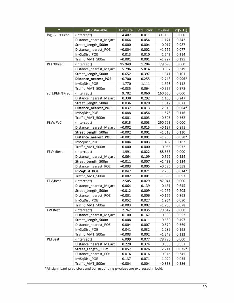
39


log.FVC %Pred (Intercept) 4.407 0.011 391.189 0.000


Street_Length_500m 0.000 0.004 0.017 0.987


InvSqDist_POE 0.013 0.010 1.243 0.214

Traffic_VMT_500m −0.001 0.001 −1.297 0.195

PEF %Pred (Intercept) 95.949 1.204 79.693 0.000


Street_Length_500m −0.652 0.397 −1.641 0.101


InvSqDist_POE 1.770 1.111 1.593 0.112

Traffic_VMT_500m −0.035 0.064 −0.557 0.578

sqrt.PEF %Pred (Intercept) 9.702 0.060 160.660 0.000


Street_Length_500m −0.036 0.020 −1.812 0.071


InvSqDist_POE 0.088 0.056 1.575 0.116

Traffic_VMT_500m −0.001 0.003 −0.303 0.762

FEV1/FVC (Intercept) 0.915 0.003 290.795 0.000

Distance_nearest_Majart −0.002 0.015 −0.137 0.891

Street_Length_500m −0.002 0.001 −1.518 0.130


InvSqDist_POE 0.004 0.003 1.402 0.162

Traffic_VMT_500m 0.000 0.000 0.035 0.972

FEV0.5Best (Intercept) 1.991 0.022 88.556 0.000


Street_Length_500m −0.011 0.007 −1.499 0.134


InvSqDist_POE 0.047 0.021 2.266 0.024*

Traffic_VMT_500m −0.002 0.001 −1.683 0.093

FEV1Best (Intercept) 2.505 0.029 87.041 0.000


Street_Length_500m −0.012 0.009 −1.269 0.205


InvSqDist_POE 0.052 0.027 1.964 0.050

Traffic_VMT_500m −0.003 0.002 −1.765 0.078

FVCBest (Intercept) 2.762 0.035 79.642 0.000


Street_Length_500m −0.008 0.011 −0.680 0.497


InvSqDist_POE 0.041 0.032 1.289 0.198

Traffic_VMT_500m −0.003 0.002 −1.549 0.122

PEFBest (Intercept) 6.099 0.077 78.796 0.000


Street_Length_500m −0.057 0.026 −2.241 0.025*


InvSqDist_POE 0.137 0.071 1.920 0.055

Traffic_VMT_500m −0.004 0.004 −0.868 0.386

*All significant predictors and corresponding p-values are expressed in bold.

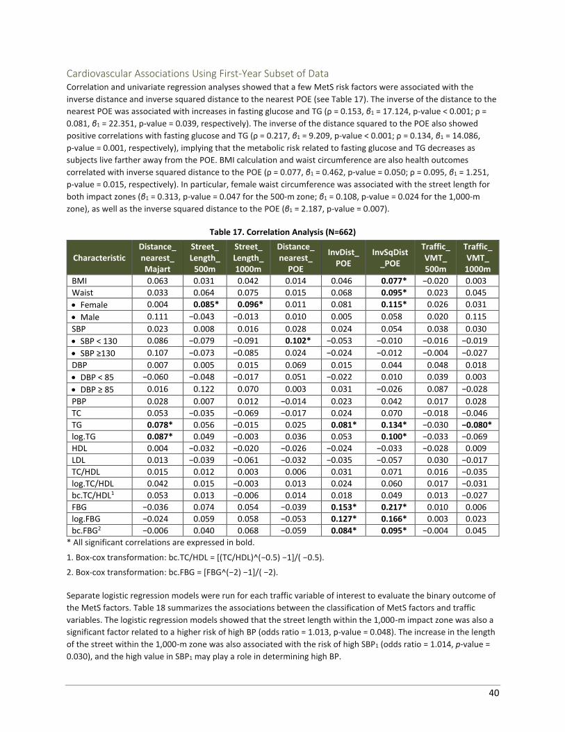
40

Cardiovascular Associations Using First-Year Subset of Data Correlation and univariate regression analyses showed that a few MetS risk factors were associated with the

inverse distance and inverse squared distance to the nearest POE (see Table 17). The inverse of the distance to the

nearest POE was associated with increases in fasting glucose and TG (ρ = 0.153, β1 = 17.124, p-value < 0.001; ρ =

0.081, β1 = 22.351, p-value = 0.039, respectively). The inverse of the distance squared to the POE also showed

positive correlations with fasting glucose and TG (ρ = 0.217, β1 = 9.209, p-value < 0.001; ρ = 0.134, β1 = 14.086,

p-value = 0.001, respectively), implying that the metabolic risk related to fasting glucose and TG decreases as

subjects live farther away from the POE. BMI calculation and waist circumference are also health outcomes

correlated with inverse squared distance to the POE (ρ = 0.077, β1 = 0.462, p-value = 0.050; ρ = 0.095, β1 = 1.251,

p-value = 0.015, respectively). In particular, female waist circumference was associated with the street length for

both impact zones (β1 = 0.313, p-value = 0.047 for the 500-m zone; β1 = 0.108, p-value = 0.024 for the 1,000-m

zone), as well as the inverse squared distance to the POE (β1 = 2.187, p-value = 0.007).

Table 17. Correlation Analysis (N=662)

Characteristic Distance_ nearest_ Majart

Street_ Length_

500m


Distance_ nearest_

POE

InvDist_ POE

InvSqDist _POE

Traffic_ VMT_ 500m

Traffic_ VMT_ 1000m

BMI 0.063 0.031 0.042 0.014 0.046 0.077* −0.020 0.003

Waist 0.033 0.064 0.075 0.015 0.068 0.095* 0.023 0.045

• Female 0.004 0.085* 0.096* 0.011 0.081 0.115* 0.026 0.031

• Male 0.111 −0.043 −0.013 0.010 0.005 0.058 0.020 0.115

SBP 0.023 0.008 0.016 0.028 0.024 0.054 0.038 0.030

• SBP < 130 0.086 −0.079 −0.091 0.102* −0.053 −0.010 −0.016 −0.019

• SBP ≥130 0.107 −0.073 −0.085 0.024 −0.024 −0.012 −0.004 −0.027

DBP 0.007 0.005 0.015 0.069 0.015 0.044 0.048 0.018

• DBP < 85 −0.060 −0.048 −0.017 0.051 −0.022 0.010 0.039 0.003

• DBP ≥ 85 0.016 0.122 0.070 0.003 0.031 −0.026 0.087 −0.028

PBP 0.028 0.007 0.012 −0.014 0.023 0.042 0.017 0.028

TC 0.053 −0.035 −0.069 −0.017 0.024 0.070 −0.018 −0.046

TG 0.078* 0.056 −0.015 0.025 0.081* 0.134* −0.030 −0.080*

log.TG 0.087* 0.049 −0.003 0.036 0.053 0.100* −0.033 −0.069

HDL 0.004 −0.032 −0.020 −0.026 −0.024 −0.033 −0.028 0.009

LDL 0.013 −0.039 −0.061 −0.032 −0.035 −0.057 0.030 −0.017

TC/HDL 0.015 0.012 0.003 0.006 0.031 0.071 0.016 −0.035

log.TC/HDL 0.042 0.015 −0.003 0.013 0.024 0.060 0.017 −0.031

bc.TC/HDL1 0.053 0.013 −0.006 0.014 0.018 0.049 0.013 −0.027

FBG −0.036 0.074 0.054 −0.039 0.153* 0.217* 0.010 0.006

log.FBG −0.024 0.059 0.058 −0.053 0.127* 0.166* 0.003 0.023

bc.FBG2 −0.006 0.040 0.068 −0.059 0.084* 0.095* −0.004 0.045


1. Box-cox transformation: bc.TC/HDL = [(TC/HDL)^(−0.5) −1]/( −0.5).

2. Box-cox transformation: bc.FBG = [FBG^(−2) −1]/( −2).

Separate logistic regression models were run for each traffic variable of interest to evaluate the binary outcome of

the MetS factors. Table 18 summarizes the associations between the classification of MetS factors and traffic

variables. The logistic regression models showed that the street length within the 1,000-m impact zone was also a

significant factor related to a higher risk of high BP (odds ratio = 1.013, p-value = 0.048). The increase in the length

of the street within the 1,000-m zone was also associated with the risk of high SBP1 (odds ratio = 1.014, p-value =

0.030), and the high value in SBP1 may play a role in determining high BP.

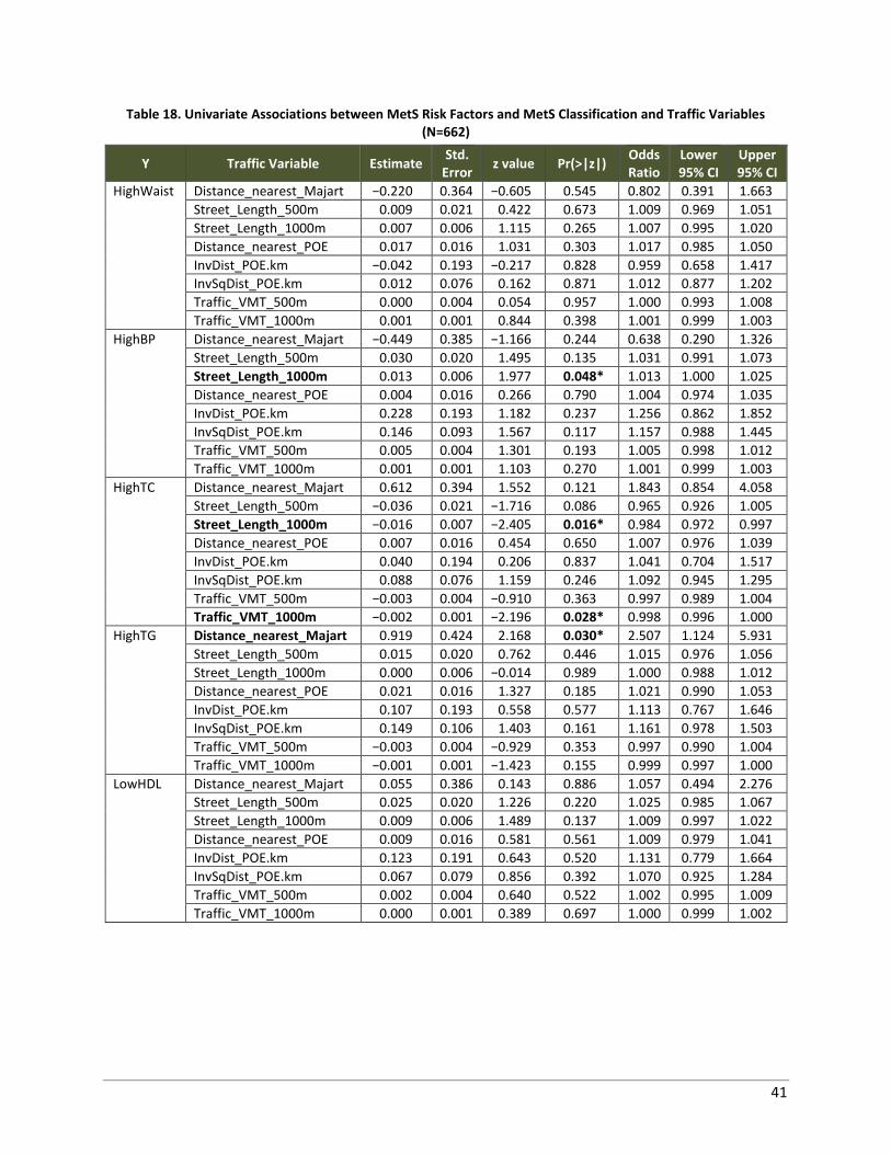
41

Table 18. Univariate Associations between MetS Risk Factors and MetS Classification and Traffic Variables (N=662)

Y Traffic Variable Estimate Std.

Error z value Pr(>|z|)

Odds Ratio

Lower 95% CI

Upper 95% CI

HighWaist Distance_nearest_Majart −0.220 0.364 −0.605 0.545 0.802 0.391 1.663

Street_Length_500m 0.009 0.021 0.422 0.673 1.009 0.969 1.051

Street_Length_1000m 0.007 0.006 1.115 0.265 1.007 0.995 1.020

Distance_nearest_POE 0.017 0.016 1.031 0.303 1.017 0.985 1.050

InvDist_POE.km −0.042 0.193 −0.217 0.828 0.959 0.658 1.417

InvSqDist_POE.km 0.012 0.076 0.162 0.871 1.012 0.877 1.202

Traffic_VMT_500m 0.000 0.004 0.054 0.957 1.000 0.993 1.008

Traffic_VMT_1000m 0.001 0.001 0.844 0.398 1.001 0.999 1.003

HighBP Distance_nearest_Majart −0.449 0.385 −1.166 0.244 0.638 0.290 1.326

Street_Length_500m 0.030 0.020 1.495 0.135 1.031 0.991 1.073

Street_Length_1000m 0.013 0.006 1.977 0.048* 1.013 1.000 1.025


InvDist_POE.km 0.228 0.193 1.182 0.237 1.256 0.862 1.852

InvSqDist_POE.km 0.146 0.093 1.567 0.117 1.157 0.988 1.445

Traffic_VMT_500m 0.005 0.004 1.301 0.193 1.005 0.998 1.012

Traffic_VMT_1000m 0.001 0.001 1.103 0.270 1.001 0.999 1.003

HighTC Distance_nearest_Majart 0.612 0.394 1.552 0.121 1.843 0.854 4.058

Street_Length_500m −0.036 0.021 −1.716 0.086 0.965 0.926 1.005

Street_Length_1000m −0.016 0.007 −2.405 0.016* 0.984 0.972 0.997


InvDist_POE.km 0.040 0.194 0.206 0.837 1.041 0.704 1.517

InvSqDist_POE.km 0.088 0.076 1.159 0.246 1.092 0.945 1.295

Traffic_VMT_500m −0.003 0.004 −0.910 0.363 0.997 0.989 1.004

Traffic_VMT_1000m −0.002 0.001 −2.196 0.028* 0.998 0.996 1.000

HighTG Distance_nearest_Majart 0.919 0.424 2.168 0.030* 2.507 1.124 5.931

Street_Length_500m 0.015 0.020 0.762 0.446 1.015 0.976 1.056

Street_Length_1000m 0.000 0.006 −0.014 0.989 1.000 0.988 1.012


InvDist_POE.km 0.107 0.193 0.558 0.577 1.113 0.767 1.646

InvSqDist_POE.km 0.149 0.106 1.403 0.161 1.161 0.978 1.503

Traffic_VMT_500m −0.003 0.004 −0.929 0.353 0.997 0.990 1.004

Traffic_VMT_1000m −0.001 0.001 −1.423 0.155 0.999 0.997 1.000

LowHDL Distance_nearest_Majart 0.055 0.386 0.143 0.886 1.057 0.494 2.276

Street_Length_500m 0.025 0.020 1.226 0.220 1.025 0.985 1.067

Street_Length_1000m 0.009 0.006 1.489 0.137 1.009 0.997 1.022


InvDist_POE.km 0.123 0.191 0.643 0.520 1.131 0.779 1.664

InvSqDist_POE.km 0.067 0.079 0.856 0.392 1.070 0.925 1.284

Traffic_VMT_500m 0.002 0.004 0.640 0.522 1.002 0.995 1.009

Traffic_VMT_1000m 0.000 0.001 0.389 0.697 1.000 0.999 1.002

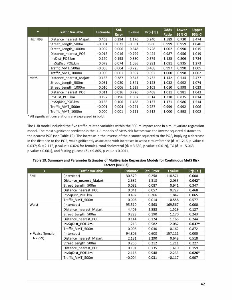
42



Odds Ratio

Lower 95% CI

Upper 95% CI

HighFBG Distance_nearest_Majart 0.463 0.394 1.176 0.240 1.589 0.730 3.474

Street_Length_500m −0.001 0.021 −0.051 0.960 0.999 0.959 1.040

Street_Length_1000m 0.002 0.006 0.348 0.728 1.002 0.990 1.015

Distance_nearest_POE −0.013 0.016 −0.799 0.424 0.987 0.956 1.019

InvDist_POE.km 0.170 0.193 0.880 0.379 1.185 0.806 1.734

InvSqDist_POE.km 0.078 0.074 1.056 0.291 1.081 0.935 1.273

Traffic_VMT_500m −0.003 0.004 −0.725 0.468 0.997 0.990 1.005

Traffic_VMT_1000m 0.000 0.001 0.397 0.692 1.000 0.998 1.002

MetS Distance_nearest_Majart 0.133 0.387 0.343 0.732 1.142 0.534 2.477

Street_Length_500m 0.031 0.020 1.541 0.123 1.032 0.992 1.074

Street_Length_1000m 0.010 0.006 1.629 0.103 1.010 0.998 1.023


InvDist_POE.km 0.197 0.196 1.007 0.314 1.218 0.835 1.814

InvSqDist_POE.km 0.158 0.106 1.488 0.137 1.171 0.986 1.514

Traffic_VMT_500m −0.001 0.004 −0.271 0.787 0.999 0.992 1.006

Traffic_VMT_1000m 0.000 0.001 0.111 0.912 1.000 0.998 1.002


The LUR model included the five traffic-related variables within the 500-m impact zone in a multivariate regression

model. The most significant predictor in the LUR models of MetS risk factors was the inverse squared distance to

the nearest POE (see Table 19). The increase in the inverse of the distance squared to the POE, implying a decrease

in the distance to the POE, was significantly associated with increases in waist circumference (β1 = 1.216, p-value =

0.037; β1 = 2.116, p-value = 0.026 for female), total cholesterol (β1 = 3.689, p-value = 0.019), TG (β1 = 15.063,

p-value = 0.001), and fasting glucose (β1 = 9.805, p-value < 0.001).

Table 19. Summary and Parameter Estimates of Multivariate Regression Models for Continuous MetS Risk Factors (N=662)


BMI (Intercept) 30.579 0.258 118.571 0.000

Distance_nearest_Majart 2.682 1.318 2.035 0.042*

Street_Length_500m 0.082 0.087 0.941 0.347


InvSqDist_POE.km 0.492 0.266 1.847 0.065

Traffic_VMT_500m −0.008 0.014 −0.558 0.577

Waist (Intercept) 95.510 0.563 169.567 0.000


Street_Length_500m 0.223 0.190 1.170 0.243


InvSqDist_POE.km 1.216 0.582 2.087 0.037*

Traffic_VMT_500m 0.005 0.030 0.162 0.872


(Intercept) 94.806 0.603 157.111 0.000


Street_Length_500m 0.256 0.212 1.211 0.227


InvSqDist_POE.km 2.116 0.948 2.233 0.026*

Traffic_VMT_500m −0.004 0.031 −0.117 0.907

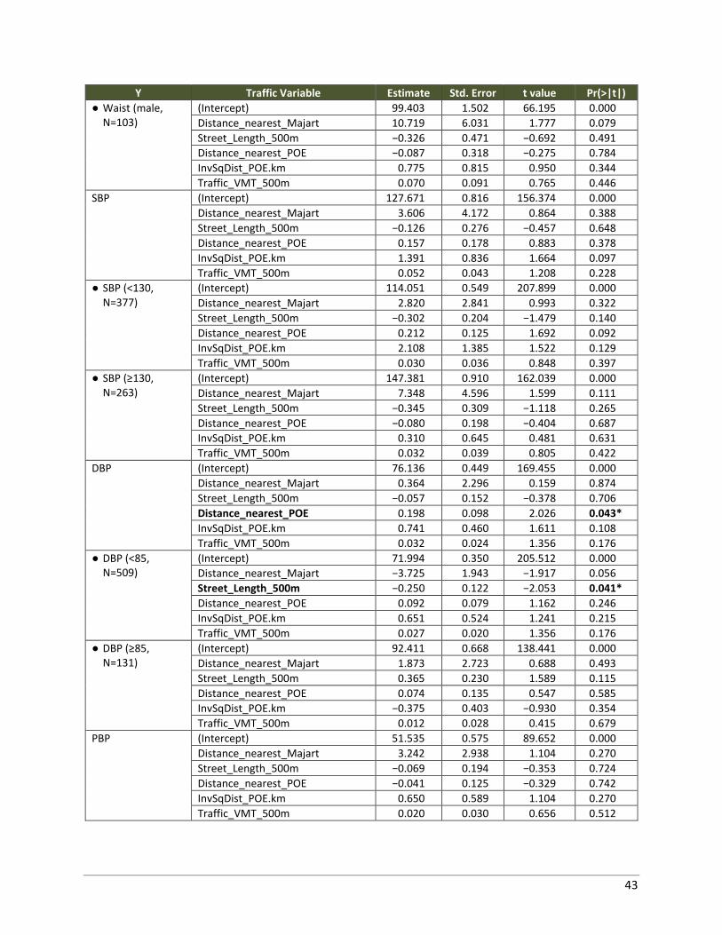
43



(Intercept) 99.403 1.502 66.195 0.000


Street_Length_500m −0.326 0.471 −0.692 0.491


InvSqDist_POE.km 0.775 0.815 0.950 0.344

Traffic_VMT_500m 0.070 0.091 0.765 0.446

SBP (Intercept) 127.671 0.816 156.374 0.000


Street_Length_500m −0.126 0.276 −0.457 0.648


InvSqDist_POE.km 1.391 0.836 1.664 0.097

Traffic_VMT_500m 0.052 0.043 1.208 0.228

● SBP (<130, N=377)

(Intercept) 114.051 0.549 207.899 0.000


Street_Length_500m −0.302 0.204 −1.479 0.140


InvSqDist_POE.km 2.108 1.385 1.522 0.129

Traffic_VMT_500m 0.030 0.036 0.848 0.397

● SBP (≥130, N=263)

(Intercept) 147.381 0.910 162.039 0.000


Street_Length_500m −0.345 0.309 −1.118 0.265


InvSqDist_POE.km 0.310 0.645 0.481 0.631

Traffic_VMT_500m 0.032 0.039 0.805 0.422

DBP (Intercept) 76.136 0.449 169.455 0.000


Street_Length_500m −0.057 0.152 −0.378 0.706

Distance_nearest_POE 0.198 0.098 2.026 0.043*

InvSqDist_POE.km 0.741 0.460 1.611 0.108

Traffic_VMT_500m 0.032 0.024 1.356 0.176

● DBP (<85, N=509)

(Intercept) 71.994 0.350 205.512 0.000


Street_Length_500m −0.250 0.122 −2.053 0.041*


InvSqDist_POE.km 0.651 0.524 1.241 0.215

Traffic_VMT_500m 0.027 0.020 1.356 0.176

● DBP (≥85, N=131)

(Intercept) 92.411 0.668 138.441 0.000


Street_Length_500m 0.365 0.230 1.589 0.115


InvSqDist_POE.km −0.375 0.403 −0.930 0.354

Traffic_VMT_500m 0.012 0.028 0.415 0.679

PBP (Intercept) 51.535 0.575 89.652 0.000


Street_Length_500m −0.069 0.194 −0.353 0.724


InvSqDist_POE.km 0.650 0.589 1.104 0.270

Traffic_VMT_500m 0.020 0.030 0.656 0.512

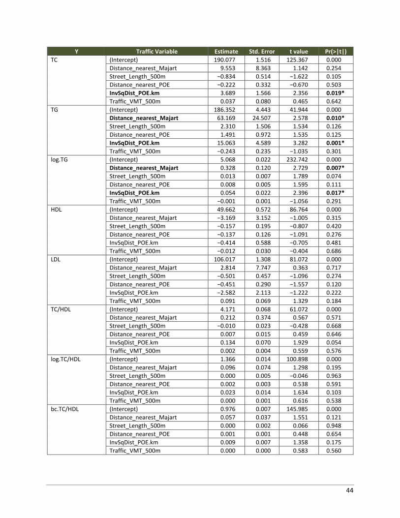
44


TC (Intercept) 190.077 1.516 125.367 0.000


Street_Length_500m −0.834 0.514 −1.622 0.105


InvSqDist_POE.km 3.689 1.566 2.356 0.019*

Traffic_VMT_500m 0.037 0.080 0.465 0.642

TG (Intercept) 186.352 4.443 41.944 0.000


Street_Length_500m 2.310 1.506 1.534 0.126


InvSqDist_POE.km 15.063 4.589 3.282 0.001*

Traffic_VMT_500m −0.243 0.235 −1.035 0.301

log.TG (Intercept) 5.068 0.022 232.742 0.000


Street_Length_500m 0.013 0.007 1.789 0.074


InvSqDist_POE.km 0.054 0.022 2.396 0.017*

Traffic_VMT_500m −0.001 0.001 −1.056 0.291

HDL (Intercept) 49.662 0.572 86.764 0.000


Street_Length_500m −0.157 0.195 −0.807 0.420


InvSqDist_POE.km −0.414 0.588 −0.705 0.481

Traffic_VMT_500m −0.012 0.030 −0.404 0.686

LDL (Intercept) 106.017 1.308 81.072 0.000


Street_Length_500m −0.501 0.457 −1.096 0.274


InvSqDist_POE.km −2.582 2.113 −1.222 0.222

Traffic_VMT_500m 0.091 0.069 1.329 0.184

TC/HDL (Intercept) 4.171 0.068 61.072 0.000


Street_Length_500m −0.010 0.023 −0.428 0.668


InvSqDist_POE.km 0.134 0.070 1.929 0.054

Traffic_VMT_500m 0.002 0.004 0.559 0.576

log.TC/HDL (Intercept) 1.366 0.014 100.898 0.000


Street_Length_500m 0.000 0.005 −0.046 0.963


InvSqDist_POE.km 0.023 0.014 1.634 0.103

Traffic_VMT_500m 0.000 0.001 0.616 0.538

bc.TC/HDL (Intercept) 0.976 0.007 145.985 0.000


Street_Length_500m 0.000 0.002 0.066 0.948


InvSqDist_POE.km 0.009 0.007 1.358 0.175

Traffic_VMT_500m 0.000 0.000 0.583 0.560

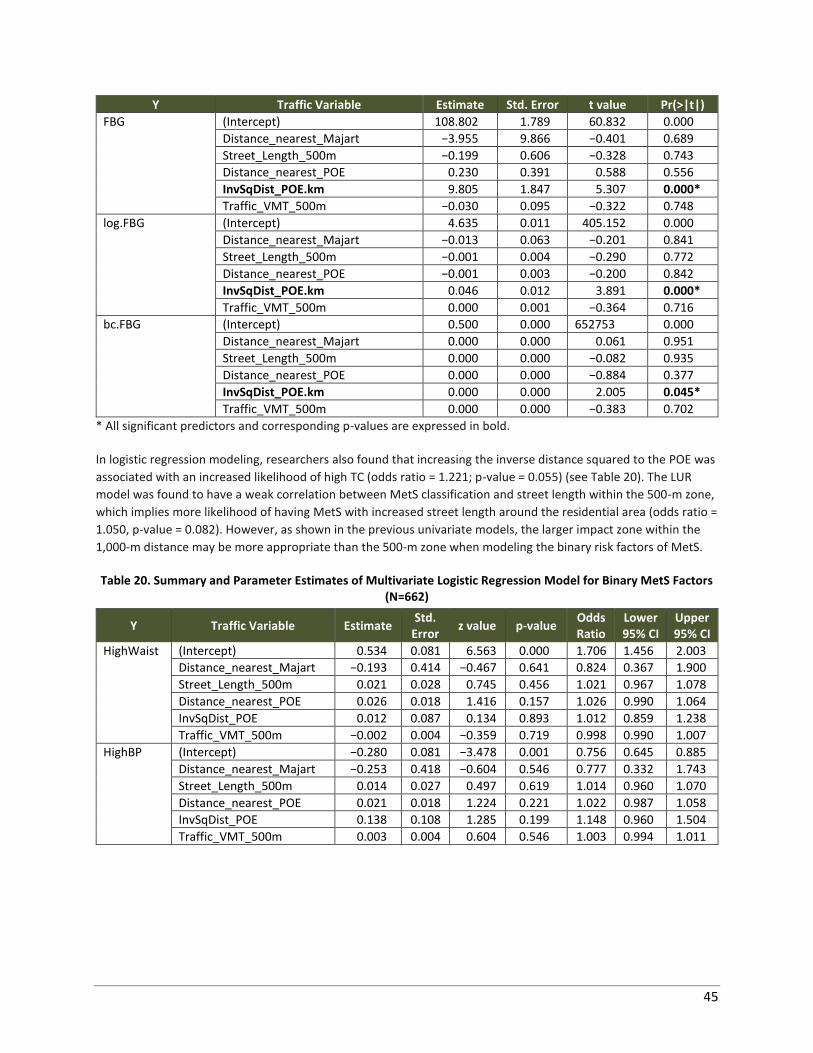
45


FBG (Intercept) 108.802 1.789 60.832 0.000


Street_Length_500m −0.199 0.606 −0.328 0.743


InvSqDist_POE.km 9.805 1.847 5.307 0.000*

Traffic_VMT_500m −0.030 0.095 −0.322 0.748

log.FBG (Intercept) 4.635 0.011 405.152 0.000


Street_Length_500m −0.001 0.004 −0.290 0.772


InvSqDist_POE.km 0.046 0.012 3.891 0.000*

Traffic_VMT_500m 0.000 0.001 −0.364 0.716

bc.FBG (Intercept) 0.500 0.000 652753 0.000


Street_Length_500m 0.000 0.000 −0.082 0.935


InvSqDist_POE.km 0.000 0.000 2.005 0.045*

Traffic_VMT_500m 0.000 0.000 −0.383 0.702

* All significant predictors and corresponding p-values are expressed in bold.

In logistic regression modeling, researchers also found that increasing the inverse distance squared to the POE was

associated with an increased likelihood of high TC (odds ratio = 1.221; p-value = 0.055) (see Table 20). The LUR

model was found to have a weak correlation between MetS classification and street length within the 500-m zone,

which implies more likelihood of having MetS with increased street length around the residential area (odds ratio =

1.050, p-value = 0.082). However, as shown in the previous univariate models, the larger impact zone within the

1,000-m distance may be more appropriate than the 500-m zone when modeling the binary risk factors of MetS.

Table 20. Summary and Parameter Estimates of Multivariate Logistic Regression Model for Binary MetS Factors (N=662)


Error z value p-value

Odds Ratio

Lower 95% CI

Upper 95% CI

HighWaist (Intercept) 0.534 0.081 6.563 0.000 1.706 1.456 2.003

Distance_nearest_Majart −0.193 0.414 −0.467 0.641 0.824 0.367 1.900

Street_Length_500m 0.021 0.028 0.745 0.456 1.021 0.967 1.078


InvSqDist_POE 0.012 0.087 0.134 0.893 1.012 0.859 1.238

Traffic_VMT_500m −0.002 0.004 −0.359 0.719 0.998 0.990 1.007

HighBP (Intercept) −0.280 0.081 −3.478 0.001 0.756 0.645 0.885


Street_Length_500m 0.014 0.027 0.497 0.619 1.014 0.960 1.070


InvSqDist_POE 0.138 0.108 1.285 0.199 1.148 0.960 1.504

Traffic_VMT_500m 0.003 0.004 0.604 0.546 1.003 0.994 1.011

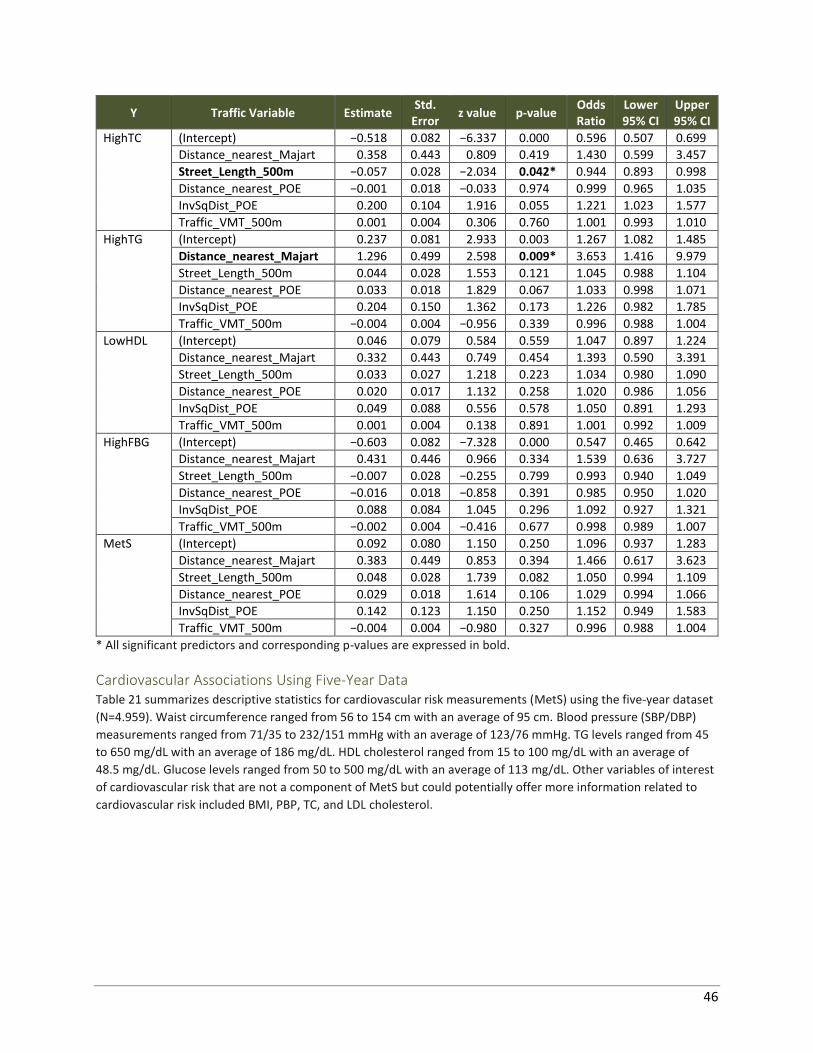
46


Error z value p-value

Odds Ratio

Lower 95% CI

Upper 95% CI

HighTC (Intercept) −0.518 0.082 −6.337 0.000 0.596 0.507 0.699

Distance_nearest_Majart 0.358 0.443 0.809 0.419 1.430 0.599 3.457

Street_Length_500m −0.057 0.028 −2.034 0.042* 0.944 0.893 0.998


InvSqDist_POE 0.200 0.104 1.916 0.055 1.221 1.023 1.577

Traffic_VMT_500m 0.001 0.004 0.306 0.760 1.001 0.993 1.010

HighTG (Intercept) 0.237 0.081 2.933 0.003 1.267 1.082 1.485

Distance_nearest_Majart 1.296 0.499 2.598 0.009* 3.653 1.416 9.979

Street_Length_500m 0.044 0.028 1.553 0.121 1.045 0.988 1.104


InvSqDist_POE 0.204 0.150 1.362 0.173 1.226 0.982 1.785

Traffic_VMT_500m −0.004 0.004 −0.956 0.339 0.996 0.988 1.004

LowHDL (Intercept) 0.046 0.079 0.584 0.559 1.047 0.897 1.224


Street_Length_500m 0.033 0.027 1.218 0.223 1.034 0.980 1.090


InvSqDist_POE 0.049 0.088 0.556 0.578 1.050 0.891 1.293

Traffic_VMT_500m 0.001 0.004 0.138 0.891 1.001 0.992 1.009

HighFBG (Intercept) −0.603 0.082 −7.328 0.000 0.547 0.465 0.642


Street_Length_500m −0.007 0.028 −0.255 0.799 0.993 0.940 1.049


InvSqDist_POE 0.088 0.084 1.045 0.296 1.092 0.927 1.321

Traffic_VMT_500m −0.002 0.004 −0.416 0.677 0.998 0.989 1.007

MetS (Intercept) 0.092 0.080 1.150 0.250 1.096 0.937 1.283


Street_Length_500m 0.048 0.028 1.739 0.082 1.050 0.994 1.109


InvSqDist_POE 0.142 0.123 1.150 0.250 1.152 0.949 1.583

Traffic_VMT_500m −0.004 0.004 −0.980 0.327 0.996 0.988 1.004


Cardiovascular Associations Using Five-Year Data Table 21 summarizes descriptive statistics for cardiovascular risk measurements (MetS) using the five-year dataset

(N=4.959). Waist circumference ranged from 56 to 154 cm with an average of 95 cm. Blood pressure (SBP/DBP)

measurements ranged from 71/35 to 232/151 mmHg with an average of 123/76 mmHg. TG levels ranged from 45

to 650 mg/dL with an average of 186 mg/dL. HDL cholesterol ranged from 15 to 100 mg/dL with an average of

48.5 mg/dL. Glucose levels ranged from 50 to 500 mg/dL with an average of 113 mg/dL. Other variables of interest

of cardiovascular risk that are not a component of MetS but could potentially offer more information related to

cardiovascular risk included BMI, PBP, TC, and LDL cholesterol.

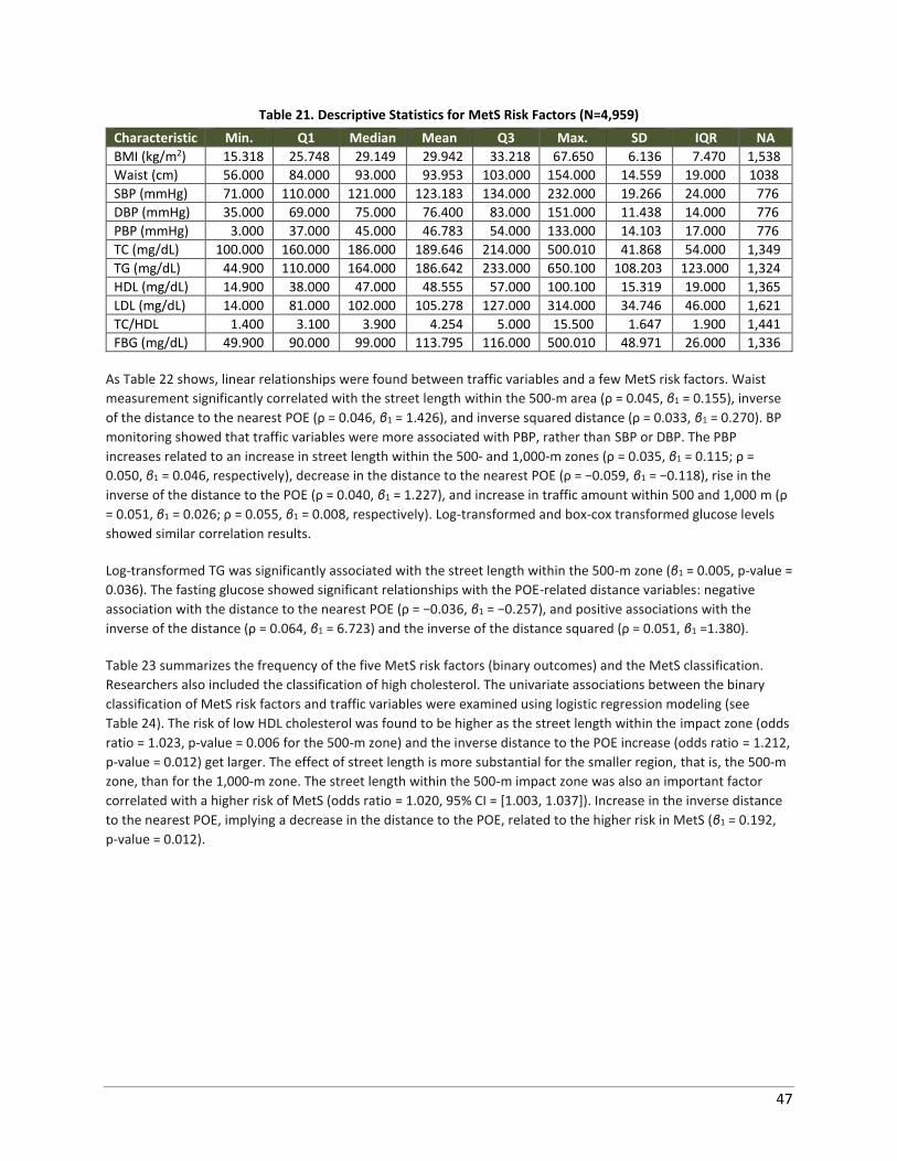
47

Table 21. Descriptive Statistics for MetS Risk Factors (N=4,959)

Characteristic Min. Q1 Median Mean Q3 Max. SD IQR NA

BMI (kg/m2) 15.318 25.748 29.149 29.942 33.218 67.650 6.136 7.470 1,538

Waist (cm) 56.000 84.000 93.000 93.953 103.000 154.000 14.559 19.000 1038

SBP (mmHg) 71.000 110.000 121.000 123.183 134.000 232.000 19.266 24.000 776

DBP (mmHg) 35.000 69.000 75.000 76.400 83.000 151.000 11.438 14.000 776

PBP (mmHg) 3.000 37.000 45.000 46.783 54.000 133.000 14.103 17.000 776

TC (mg/dL) 100.000 160.000 186.000 189.646 214.000 500.010 41.868 54.000 1,349

TG (mg/dL) 44.900 110.000 164.000 186.642 233.000 650.100 108.203 123.000 1,324

HDL (mg/dL) 14.900 38.000 47.000 48.555 57.000 100.100 15.319 19.000 1,365

LDL (mg/dL) 14.000 81.000 102.000 105.278 127.000 314.000 34.746 46.000 1,621

TC/HDL 1.400 3.100 3.900 4.254 5.000 15.500 1.647 1.900 1,441

FBG (mg/dL) 49.900 90.000 99.000 113.795 116.000 500.010 48.971 26.000 1,336

As Table 22 shows, linear relationships were found between traffic variables and a few MetS risk factors. Waist

measurement significantly correlated with the street length within the 500-m area (ρ = 0.045, β1 = 0.155), inverse

of the distance to the nearest POE (ρ = 0.046, β1 = 1.426), and inverse squared distance (ρ = 0.033, β1 = 0.270). BP

monitoring showed that traffic variables were more associated with PBP, rather than SBP or DBP. The PBP

increases related to an increase in street length within the 500- and 1,000-m zones (ρ = 0.035, β1 = 0.115; ρ =

0.050, β1 = 0.046, respectively), decrease in the distance to the nearest POE (ρ = −0.059, β1 = −0.118), rise in the

inverse of the distance to the POE (ρ = 0.040, β1 = 1.227), and increase in traffic amount within 500 and 1,000 m (ρ

= 0.051, β1 = 0.026; ρ = 0.055, β1 = 0.008, respectively). Log-transformed and box-cox transformed glucose levels

showed similar correlation results.

Log-transformed TG was significantly associated with the street length within the 500-m zone (β1 = 0.005, p-value =

0.036). The fasting glucose showed significant relationships with the POE-related distance variables: negative

association with the distance to the nearest POE (ρ = −0.036, β1 = −0.257), and positive associations with the

inverse of the distance (ρ = 0.064, β1 = 6.723) and the inverse of the distance squared (ρ = 0.051, β1 =1.380).

Table 23 summarizes the frequency of the five MetS risk factors (binary outcomes) and the MetS classification.

Researchers also included the classification of high cholesterol. The univariate associations between the binary

classification of MetS risk factors and traffic variables were examined using logistic regression modeling (see

Table 24). The risk of low HDL cholesterol was found to be higher as the street length within the impact zone (odds

ratio = 1.023, p-value = 0.006 for the 500-m zone) and the inverse distance to the POE increase (odds ratio = 1.212,

p-value = 0.012) get larger. The effect of street length is more substantial for the smaller region, that is, the 500-m

zone, than for the 1,000-m zone. The street length within the 500-m impact zone was also an important factor

correlated with a higher risk of MetS (odds ratio = 1.020, 95% CI = [1.003, 1.037]). Increase in the inverse distance

to the nearest POE, implying a decrease in the distance to the POE, related to the higher risk in MetS (β1 = 0.192,

p-value = 0.012).

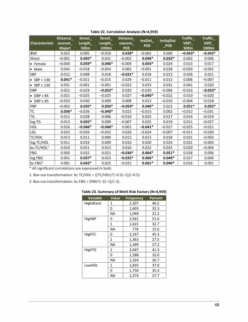
48

Table 22. Correlation Analysis (N=4,959)

Characteristic Distance_ nearest_ Majart

Street_ Length_

500m


Distance_ nearest_

POE

InvDist_ POE

InvSqDist _POE

Traffic_ VMT_ 500m

Traffic_ VMT_ 1000m

BMI 0.022 0.005 −0.010 0.039* −0.002 0.000 −0.043* −0.042*

Waist −0.001 0.045* 0.031 −0.002 0.046* 0.033* 0.002 0.006

• Female −0.004 0.059* 0.046* −0.009 0.054* 0.024 0.013 0.017

• Male 0.045 −0.018 −0.054 0.065 −0.001 0.028 −0.050 −0.062

SBP 0.012 0.008 0.018 −0.031* 0.018 0.013 0.028 0.021

• SBP < 130 0.041* −0.021 −0.015 0.029 −0.011 0.012 0.006 −0.007

• SBP ≥ 130 0.031 −0.001 −0.001 −0.022 0.033 0.031 0.041 0.020

DBP 0.022 −0.029 −0.032* 0.020 −0.020 −0.006 −0.016 −0.033*

• DBP < 85 0.021 −0.025 −0.025 0.027 −0.040* −0.022 0.010 −0.020

• DBP ≥ 85 −0.033 0.030 0.009 0.008 0.013 −0.010 −0.004 −0.018

PBP −0.002 0.035* 0.050* −0.059* 0.040* 0.023 0.051* 0.055*

TC 0.036* −0.026 −0.040* 0.022 −0.015 0.002 −0.012 −0.031

TG 0.012 0.028 0.006 −0.010 0.023 0.017 0.014 −0.019

log.TG 0.013 0.035* 0.009 −0.007 0.025 0.019 0.011 −0.027

HDL 0.016 −0.046* −0.046* 0.001 −0.041* −0.027 −0.025 −0.021

LDL 0.023 −0.026 −0.032 0.026 −0.024 −0.007 −0.011 −0.020

TC/HDL 0.013 0.011 0.000 0.012 0.013 0.018 0.021 −0.003

log.TC/HDL 0.011 0.019 0.009 0.010 0.020 0.024 0.021 −0.003

bc.TC/HDL1 0.010 0.021 0.013 0.010 0.022 0.025 0.020 −0.004

FBG 0.003 0.032 0.021 −0.036* 0.064* 0.051* 0.018 0.006

log.FBG 0.001 0.037* 0.023 −0.035* 0.066* 0.049* 0.017 0.004

bc.FBG2 0.001 0.043* 0.025 −0.031 0.061* 0.040* 0.016 0.001


1. Box-cox transformation: bc.TC/HDL = [(TC/HDL)^(−0.5)−1]/(−0.5).

2. Box-cox transformation: bc.FBG = [FBG^(−2)−1]/(−2).

Table 23. Summary of MetS Risk Factors (N=4,959)


HighWaist 1 2,307 46.5

0 1,603 32.3

NA 1,049 21.2

HighBP 0 2,561 51.6

1 1,622 32.7

NA 776 15.6

HighTC 0 2,247 45.3

1 1,363 27.5

NA 1,349 27.2

HighTG 1 2,047 41.3

0 1,588 32.0

NA 1,324 26.7

LowHDL 1 1,835 37.0

0 1,750 35.3

NA 1,374 27.7

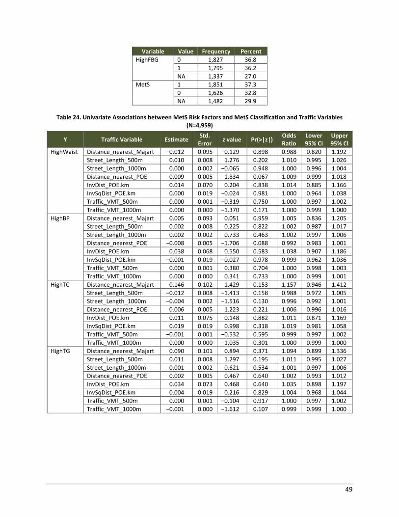
49


HighFBG 0 1,827 36.8

1 1,795 36.2

NA 1,337 27.0

MetS 1 1,851 37.3

0 1,626 32.8

NA 1,482 29.9

Table 24. Univariate Associations between MetS Risk Factors and MetS Classification and Traffic Variables (N=4,959)



Odds Ratio

Lower 95% CI

Upper 95% CI

HighWaist Distance_nearest_Majart −0.012 0.095 −0.129 0.898 0.988 0.820 1.192

Street_Length_500m 0.010 0.008 1.276 0.202 1.010 0.995 1.026

Street_Length_1000m 0.000 0.002 −0.065 0.948 1.000 0.996 1.004


InvDist_POE.km 0.014 0.070 0.204 0.838 1.014 0.885 1.166

InvSqDist_POE.km 0.000 0.019 −0.024 0.981 1.000 0.964 1.038

Traffic_VMT_500m 0.000 0.001 −0.319 0.750 1.000 0.997 1.002

Traffic_VMT_1000m 0.000 0.000 −1.370 0.171 1.000 0.999 1.000

HighBP Distance_nearest_Majart 0.005 0.093 0.051 0.959 1.005 0.836 1.205

Street_Length_500m 0.002 0.008 0.225 0.822 1.002 0.987 1.017

Street_Length_1000m 0.002 0.002 0.733 0.463 1.002 0.997 1.006


InvDist_POE.km 0.038 0.068 0.550 0.583 1.038 0.907 1.186

InvSqDist_POE.km −0.001 0.019 −0.027 0.978 0.999 0.962 1.036

Traffic_VMT_500m 0.000 0.001 0.380 0.704 1.000 0.998 1.003

Traffic_VMT_1000m 0.000 0.000 0.341 0.733 1.000 0.999 1.001

HighTC Distance_nearest_Majart 0.146 0.102 1.429 0.153 1.157 0.946 1.412

Street_Length_500m −0.012 0.008 −1.413 0.158 0.988 0.972 1.005

Street_Length_1000m −0.004 0.002 −1.516 0.130 0.996 0.992 1.001


InvDist_POE.km 0.011 0.075 0.148 0.882 1.011 0.871 1.169

InvSqDist_POE.km 0.019 0.019 0.998 0.318 1.019 0.981 1.058

Traffic_VMT_500m −0.001 0.001 −0.532 0.595 0.999 0.997 1.002

Traffic_VMT_1000m 0.000 0.000 −1.035 0.301 1.000 0.999 1.000

HighTG Distance_nearest_Majart 0.090 0.101 0.894 0.371 1.094 0.899 1.336

Street_Length_500m 0.011 0.008 1.297 0.195 1.011 0.995 1.027

Street_Length_1000m 0.001 0.002 0.621 0.534 1.001 0.997 1.006


InvDist_POE.km 0.034 0.073 0.468 0.640 1.035 0.898 1.197

InvSqDist_POE.km 0.004 0.019 0.216 0.829 1.004 0.968 1.044

Traffic_VMT_500m 0.000 0.001 −0.104 0.917 1.000 0.997 1.002

Traffic_VMT_1000m −0.001 0.000 −1.612 0.107 0.999 0.999 1.000

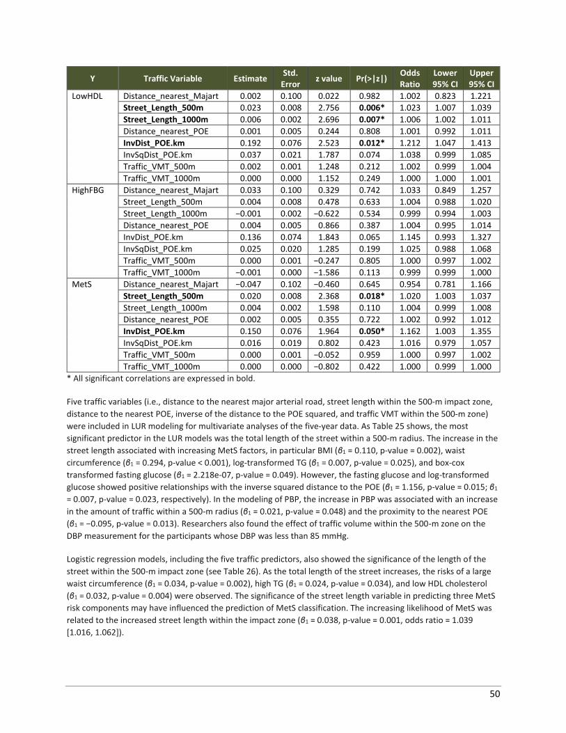
50



Odds Ratio

Lower 95% CI

Upper 95% CI

LowHDL Distance_nearest_Majart 0.002 0.100 0.022 0.982 1.002 0.823 1.221

Street_Length_500m 0.023 0.008 2.756 0.006* 1.023 1.007 1.039

Street_Length_1000m 0.006 0.002 2.696 0.007* 1.006 1.002 1.011


InvDist_POE.km 0.192 0.076 2.523 0.012* 1.212 1.047 1.413

InvSqDist_POE.km 0.037 0.021 1.787 0.074 1.038 0.999 1.085

Traffic_VMT_500m 0.002 0.001 1.248 0.212 1.002 0.999 1.004

Traffic_VMT_1000m 0.000 0.000 1.152 0.249 1.000 1.000 1.001

HighFBG Distance_nearest_Majart 0.033 0.100 0.329 0.742 1.033 0.849 1.257

Street_Length_500m 0.004 0.008 0.478 0.633 1.004 0.988 1.020

Street_Length_1000m −0.001 0.002 −0.622 0.534 0.999 0.994 1.003


InvDist_POE.km 0.136 0.074 1.843 0.065 1.145 0.993 1.327

InvSqDist_POE.km 0.025 0.020 1.285 0.199 1.025 0.988 1.068

Traffic_VMT_500m 0.000 0.001 −0.247 0.805 1.000 0.997 1.002

Traffic_VMT_1000m −0.001 0.000 −1.586 0.113 0.999 0.999 1.000

MetS Distance_nearest_Majart −0.047 0.102 −0.460 0.645 0.954 0.781 1.166

Street_Length_500m 0.020 0.008 2.368 0.018* 1.020 1.003 1.037

Street_Length_1000m 0.004 0.002 1.598 0.110 1.004 0.999 1.008


InvDist_POE.km 0.150 0.076 1.964 0.050* 1.162 1.003 1.355

InvSqDist_POE.km 0.016 0.019 0.802 0.423 1.016 0.979 1.057

Traffic_VMT_500m 0.000 0.001 −0.052 0.959 1.000 0.997 1.002

Traffic_VMT_1000m 0.000 0.000 −0.802 0.422 1.000 0.999 1.000


Five traffic variables (i.e., distance to the nearest major arterial road, street length within the 500-m impact zone,

distance to the nearest POE, inverse of the distance to the POE squared, and traffic VMT within the 500-m zone)

were included in LUR modeling for multivariate analyses of the five-year data. As Table 25 shows, the most

significant predictor in the LUR models was the total length of the street within a 500-m radius. The increase in the

street length associated with increasing MetS factors, in particular BMI (β1 = 0.110, p-value = 0.002), waist

circumference (β1 = 0.294, p-value < 0.001), log-transformed TG (β1 = 0.007, p-value = 0.025), and box-cox

transformed fasting glucose (β1 = 2.218e-07, p-value = 0.049). However, the fasting glucose and log-transformed

glucose showed positive relationships with the inverse squared distance to the POE (β1 = 1.156, p-value = 0.015; β1

= 0.007, p-value = 0.023, respectively). In the modeling of PBP, the increase in PBP was associated with an increase

in the amount of traffic within a 500-m radius (β1 = 0.021, p-value = 0.048) and the proximity to the nearest POE

(β1 = −0.095, p-value = 0.013). Researchers also found the effect of traffic volume within the 500-m zone on the

DBP measurement for the participants whose DBP was less than 85 mmHg.

Logistic regression models, including the five traffic predictors, also showed the significance of the length of the

street within the 500-m impact zone (see Table 26). As the total length of the street increases, the risks of a large

waist circumference (β1 = 0.034, p-value = 0.002), high TG (β1 = 0.024, p-value = 0.034), and low HDL cholesterol

(β1 = 0.032, p-value = 0.004) were observed. The significance of the street length variable in predicting three MetS

risk components may have influenced the prediction of MetS classification. The increasing likelihood of MetS was

related to the increased street length within the impact zone (β1 = 0.038, p-value = 0.001, odds ratio = 1.039

[1.016, 1.062]).

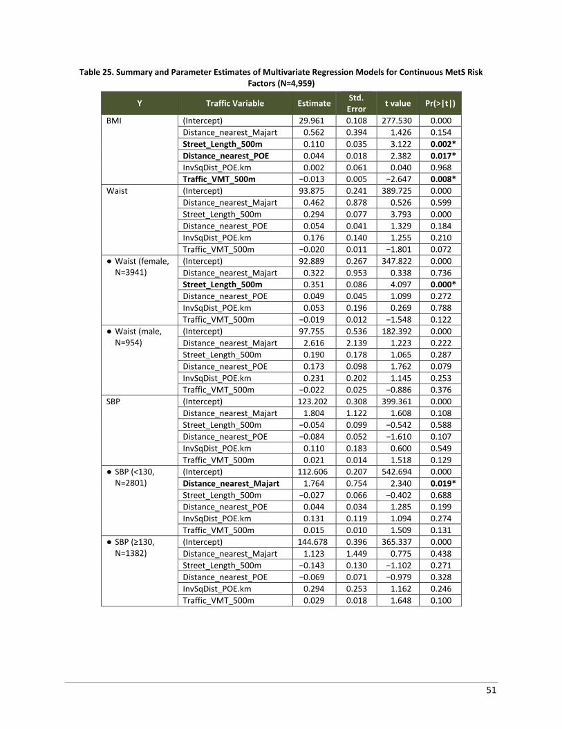
51

Table 25. Summary and Parameter Estimates of Multivariate Regression Models for Continuous MetS Risk Factors (N=4,959)


Error t value Pr(>|t|)

BMI (Intercept) 29.961 0.108 277.530 0.000


Street_Length_500m 0.110 0.035 3.122 0.002*

Distance_nearest_POE 0.044 0.018 2.382 0.017*

InvSqDist_POE.km 0.002 0.061 0.040 0.968

Traffic_VMT_500m −0.013 0.005 −2.647 0.008*

Waist (Intercept) 93.875 0.241 389.725 0.000


Street_Length_500m 0.294 0.077 3.793 0.000


InvSqDist_POE.km 0.176 0.140 1.255 0.210

Traffic_VMT_500m −0.020 0.011 −1.801 0.072


(Intercept) 92.889 0.267 347.822 0.000


Street_Length_500m 0.351 0.086 4.097 0.000*


InvSqDist_POE.km 0.053 0.196 0.269 0.788

Traffic_VMT_500m −0.019 0.012 −1.548 0.122


(Intercept) 97.755 0.536 182.392 0.000


Street_Length_500m 0.190 0.178 1.065 0.287


InvSqDist_POE.km 0.231 0.202 1.145 0.253

Traffic_VMT_500m −0.022 0.025 −0.886 0.376

SBP (Intercept) 123.202 0.308 399.361 0.000


Street_Length_500m −0.054 0.099 −0.542 0.588


InvSqDist_POE.km 0.110 0.183 0.600 0.549

Traffic_VMT_500m 0.021 0.014 1.518 0.129

● SBP (<130, N=2801)

(Intercept) 112.606 0.207 542.694 0.000


Street_Length_500m −0.027 0.066 −0.402 0.688


InvSqDist_POE.km 0.131 0.119 1.094 0.274

Traffic_VMT_500m 0.015 0.010 1.509 0.131

● SBP (≥130, N=1382)

(Intercept) 144.678 0.396 365.337 0.000


Street_Length_500m −0.143 0.130 −1.102 0.271


InvSqDist_POE.km 0.294 0.253 1.162 0.246

Traffic_VMT_500m 0.029 0.018 1.648 0.100

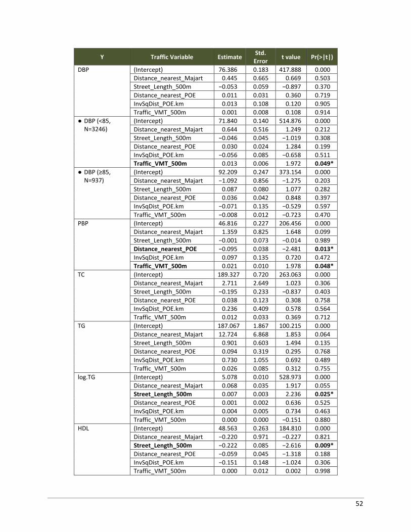
52



DBP (Intercept) 76.386 0.183 417.888 0.000


Street_Length_500m −0.053 0.059 −0.897 0.370


InvSqDist_POE.km 0.013 0.108 0.120 0.905

Traffic_VMT_500m 0.001 0.008 0.108 0.914

● DBP (<85, N=3246)

(Intercept) 71.840 0.140 514.876 0.000


Street_Length_500m −0.046 0.045 −1.019 0.308


InvSqDist_POE.km −0.056 0.085 −0.658 0.511

Traffic_VMT_500m 0.013 0.006 1.972 0.049*

● DBP (≥85, N=937)

(Intercept) 92.209 0.247 373.154 0.000


Street_Length_500m 0.087 0.080 1.077 0.282


InvSqDist_POE.km −0.071 0.135 −0.529 0.597

Traffic_VMT_500m −0.008 0.012 −0.723 0.470

PBP (Intercept) 46.816 0.227 206.456 0.000


Street_Length_500m −0.001 0.073 −0.014 0.989


InvSqDist_POE.km 0.097 0.135 0.720 0.472

Traffic_VMT_500m 0.021 0.010 1.978 0.048*

TC (Intercept) 189.327 0.720 263.063 0.000


Street_Length_500m −0.195 0.233 −0.837 0.403


InvSqDist_POE.km 0.236 0.409 0.578 0.564

Traffic_VMT_500m 0.012 0.033 0.369 0.712

TG (Intercept) 187.067 1.867 100.215 0.000


Street_Length_500m 0.901 0.603 1.494 0.135


InvSqDist_POE.km 0.730 1.055 0.692 0.489

Traffic_VMT_500m 0.026 0.085 0.312 0.755

log.TG (Intercept) 5.078 0.010 528.973 0.000


Street_Length_500m 0.007 0.003 2.236 0.025*


InvSqDist_POE.km 0.004 0.005 0.734 0.463

Traffic_VMT_500m 0.000 0.000 −0.151 0.880

HDL (Intercept) 48.563 0.263 184.810 0.000


Street_Length_500m −0.222 0.085 −2.616 0.009*


InvSqDist_POE.km −0.151 0.148 −1.024 0.306

Traffic_VMT_500m 0.000 0.012 0.002 0.998

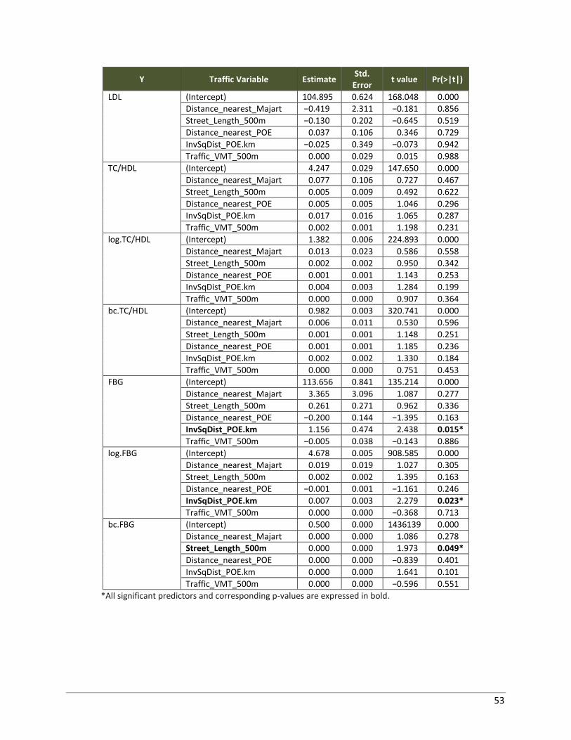
53



LDL (Intercept) 104.895 0.624 168.048 0.000


Street_Length_500m −0.130 0.202 −0.645 0.519


InvSqDist_POE.km −0.025 0.349 −0.073 0.942

Traffic_VMT_500m 0.000 0.029 0.015 0.988

TC/HDL (Intercept) 4.247 0.029 147.650 0.000


Street_Length_500m 0.005 0.009 0.492 0.622


InvSqDist_POE.km 0.017 0.016 1.065 0.287

Traffic_VMT_500m 0.002 0.001 1.198 0.231

log.TC/HDL (Intercept) 1.382 0.006 224.893 0.000


Street_Length_500m 0.002 0.002 0.950 0.342


InvSqDist_POE.km 0.004 0.003 1.284 0.199

Traffic_VMT_500m 0.000 0.000 0.907 0.364

bc.TC/HDL (Intercept) 0.982 0.003 320.741 0.000


Street_Length_500m 0.001 0.001 1.148 0.251


InvSqDist_POE.km 0.002 0.002 1.330 0.184

Traffic_VMT_500m 0.000 0.000 0.751 0.453

FBG (Intercept) 113.656 0.841 135.214 0.000


Street_Length_500m 0.261 0.271 0.962 0.336


InvSqDist_POE.km 1.156 0.474 2.438 0.015*

Traffic_VMT_500m −0.005 0.038 −0.143 0.886

log.FBG (Intercept) 4.678 0.005 908.585 0.000


Street_Length_500m 0.002 0.002 1.395 0.163


InvSqDist_POE.km 0.007 0.003 2.279 0.023*

Traffic_VMT_500m 0.000 0.000 −0.368 0.713

bc.FBG (Intercept) 0.500 0.000 1436139 0.000


Street_Length_500m 0.000 0.000 1.973 0.049*


InvSqDist_POE.km 0.000 0.000 1.641 0.101

Traffic_VMT_500m 0.000 0.000 −0.596 0.551

*All significant predictors and corresponding p-values are expressed in bold.

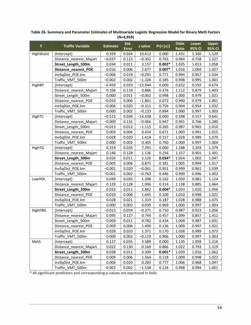
54

Table 26. Summary and Parameter Estimates of Multivariate Logistic Regression Model for Binary MetS Factors (N=4,959)



Odds Ratio

Lower 95% CI

Upper 95% CI

HighWaist (Intercept) 0.359 0.034 10.612 0.000 1.431 1.340 1.529


Street_Length_500m 0.034 0.011 3.157 0.002* 1.035 1.013 1.058

Distance_nearest_POE 0.016 0.006 2.677 0.007* 1.016 1.004 1.027

InvSqDist_POE.km −0.006 0.019 −0.291 0.771 0.994 0.957 1.034

Traffic_VMT_500m −0.002 0.002 −1.326 0.185 0.998 0.995 1.001

HighBP (Intercept) −0.459 0.033 −13.944 0.000 0.632 0.592 0.674


Street_Length_500m 0.000 0.011 −0.002 0.998 1.000 0.979 1.021


InvSqDist_POE.km −0.006 0.020 −0.311 0.756 0.994 0.954 1.032

Traffic_VMT_500m 0.000 0.002 −0.133 0.894 1.000 0.997 1.003

HighTC (Intercept) −0.515 0.036 −14.438 0.000 0.598 0.557 0.641


Street_Length_500m −0.013 0.012 −1.115 0.265 0.987 0.965 1.010


InvSqDist_POE.km 0.028 0.020 1.414 0.157 1.028 0.989 1.070

Traffic_VMT_500m 0.000 0.002 0.305 0.760 1.000 0.997 1.004

HighTG (Intercept) 0.253 0.035 7.291 0.000 1.288 1.203 1.379


Street_Length_500m 0.024 0.011 2.120 0.034* 1.024 1.002 1.047


InvSqDist_POE.km −0.001 0.020 −0.061 0.951 0.999 0.961 1.039

Traffic_VMT_500m −0.001 0.002 −0.763 0.446 0.999 0.996 1.002

LowHDL (Intercept) 0.049 0.035 1.398 0.162 1.050 0.981 1.124


Street_Length_500m 0.032 0.011 2.862 0.004* 1.033 1.010 1.056


InvSqDist_POE.km 0.028 0.021 1.319 0.187 1.028 0.988 1.075

Traffic_VMT_500m 0.000 0.002 0.039 0.969 1.000 0.997 1.003

HighFBG (Intercept) −0.013 0.034 −0.371 0.710 0.987 0.923 1.056


Street_Length_500m 0.009 0.011 0.782 0.434 1.009 0.987 1.031


InvSqDist_POE.km 0.028 0.020 1.371 0.170 1.028 0.989 1.073

Traffic_VMT_500m 0.000 0.002 −0.119 0.906 1.000 0.997 1.003

MetS (Intercept) 0.127 0.035 3.589 0.000 1.135 1.059 1.216


Street_Length_500m 0.038 0.011 3.309 0.001* 1.039 1.016 1.062


InvSqDist_POE.km 0.006 0.020 0.283 0.777 1.006 0.968 1.047

Traffic_VMT_500m −0.002 0.002 −1.538 0.124 0.998 0.994 1.001


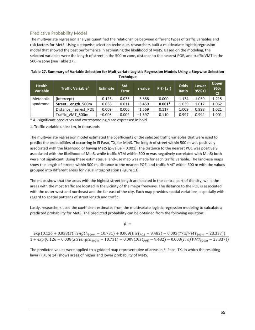
55

Predictive Probability Model The multivariate regression analysis quantified the relationships between different types of traffic variables and

risk factors for MetS. Using a stepwise selection technique, researchers built a multivariate logistic regression

model that showed the best performance in estimating the likelihood of MetS. Based on the modeling, the

selected variables were the length of street in the 500-m zone, distance to the nearest POE, and traffic VMT in the

500-m zone (see Table 27).

Table 27. Summary of Variable Selection for Multivariate Logistic Regression Models Using a Stepwise Selection Technique

Health Variable

Traffic Variable1 Estimate Std.


Odds Ratio

Lower 95% CI

Upper 95%

CI

Metabolic syndrome

(Intercept) 0.126 0.035 3.586 0.000 1.134 1.059 1.215

Street_Length_500m 0.038 0.011 3.459 0.001* 1.039 1.017 1.062


Traffic_VMT_500m −0.003 0.002 −1.597 0.110 0.997 0.994 1.001

* All significant predictors and corresponding p are expressed in bold.

1. Traffic variable units: km, in thousands

The multivariate regression model estimated the coefficients of the selected traffic variables that were used to

predict the probabilities of occurring in El Paso, TX, for MetS. The length of street within 500 m was positively

associated with the likelihood of having MetS (p-value = 0.001). The distance to the nearest POE was positively

associated with the likelihood of MetS, while traffic VTM within 500 m was negatively correlated with MetS; both

were not significant. Using these estimates, a land-use map was made for each traffic variable. The land-use maps

show the length of streets within 500 m, distance to the nearest POE, and traffic VMT within 500 m with the values

grouped into different areas for visual interpretation (Figure 13).

The maps show that the areas with the highest street length are located in the central part of the city, while the

areas with the most traffic are located in the vicinity of the major freeways. The distance to the POE is associated

with the outer west and northeast and the far east of the city. Each map provides spatial variations, especially with

regard to spatial patterns of street length and traffic.

Lastly, researchers used the coefficient estimates from the multivariate logistic regression modeling to calculate a

predicted probability for MetS. The predicted probability can be obtained from the following equation:

�̂� =

exp {0.126 + 0.038(𝑆𝑡𝑟𝑙𝑒𝑛𝑔𝑡ℎ500𝑚 − 10.731) + 0.009(𝐷𝑖𝑠𝑡𝑃𝑂𝐸 − 9.482) − 0.003(𝑇𝑟𝑎𝑓𝑉𝑀𝑇500𝑚 − 23.337)}

1 + exp {0.126 + 0.038(𝑆𝑡𝑟𝑙𝑒𝑛𝑔𝑡ℎ500𝑚 − 10.731) + 0.009(𝐷𝑖𝑠𝑡𝑃𝑂𝐸 − 9.482) − 0.003(𝑇𝑟𝑎𝑓𝑉𝑀𝑇500𝑚 − 23.337)}

The predicted values were applied to a gridded map representative of areas in El Paso, TX, in which the resulting

layer (Figure 14) shows areas of higher and lower probability of MetS.

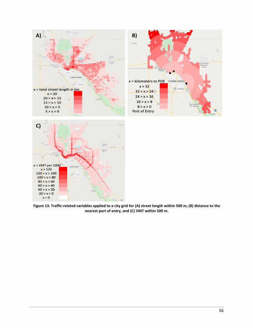
56

Figure 13. Traffic-related variables applied to a city grid for (A) street length within 500 m, (B) distance to the nearest port of entry, and (C) VMT within 500 m.

A) B)

C)

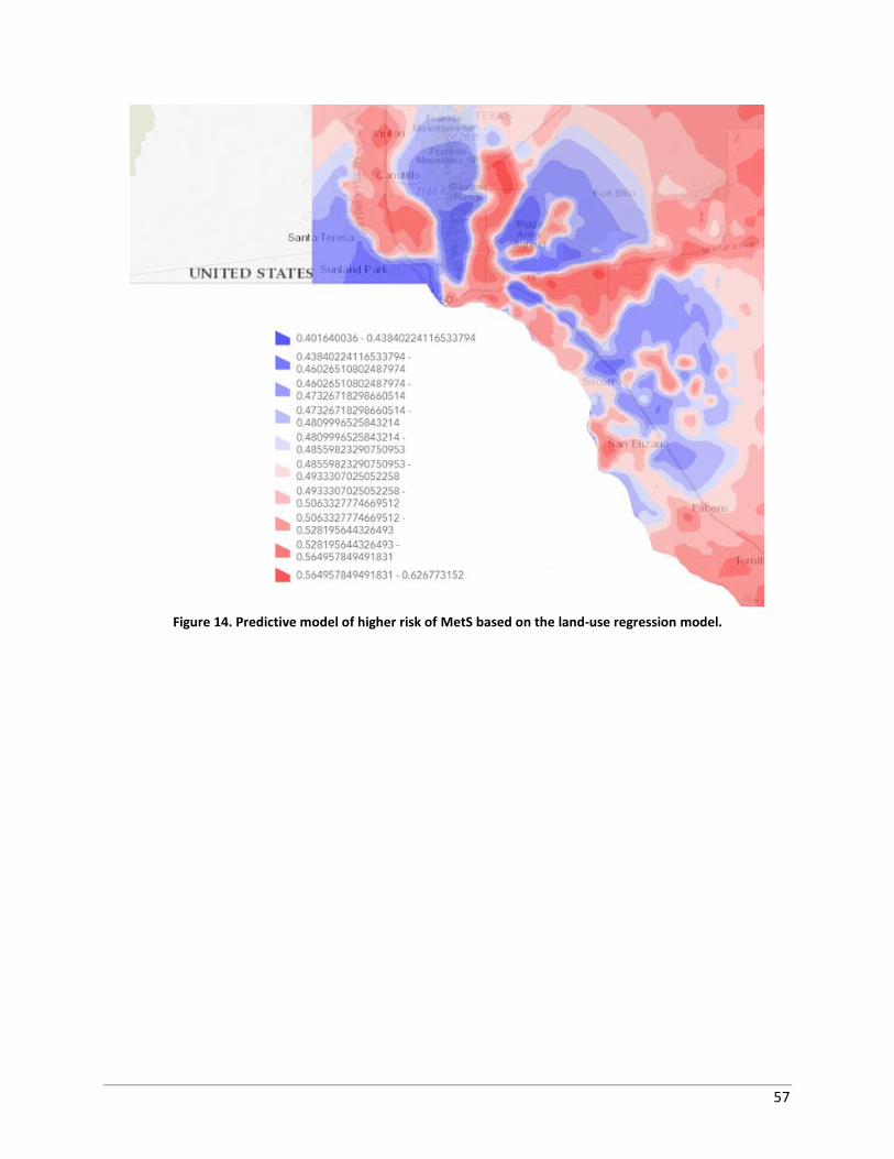
57

Figure 14. Predictive model of higher risk of MetS based on the land-use regression model.

58

Conclusions and Recommendations

Short-Term Effects of Traffic-Related Air Pollution on Cardiorespiratory Outcomes This study examined the short-term associations (24-, 48-, 72-, and 96-hr averages) of traffic-related air pollutants

(PM2.5, PM10, NO2, and O3) with biomarkers of respiratory and cardiovascular disease in a group of uninsured

participants from low-income communities in El Paso, TX. Researchers found associations of short-term air

pollutant concentrations with respiratory outcomes, which was expected. However, researchers also found

associations with metabolic risk factors such as BMI, waist circumference, and fasting glucose.

FEV1 was negatively correlated with average concentration levels of PM2.5 (24, 48, and 96 hr), indicating a

relationship between lung function and ambient PM2.5 before the measurement. Specifically, this respiratory

indicator represents an increase of risk to developing chronic obstructive pulmonary disease (COPD). Furthermore,

PEF, which is also an indicator of the respiratory risk of COPD, was negatively correlated not only with PM2.5 but

also NO2. However, researchers did not see an influence by coarse particles (PM10), which might indicate the

significant effects came from smaller particles, which affect the lower respiratory tract and can further cause

obstructive disease. Further analysis using the best results available for respiratory indicators (FEV1, FVC, and PEF),

as interpreted by the spirometry software (CareFusion Spirometry PC Software™ [36-SPC1000-STK]), further

confirmed the associations with PM2.5 air pollutants and NO2.

eNO is a measure of airway inflammation and useful in the treatment and adherence of asthma treatment but was

not correlated with concentration levels of air pollutants in the selected population. Given that the inclusion

methods do not ask if a participant has asthma, researchers cannot subset the data to explore if a relationship

exists in this subgroup. Also, based on the lung function parameter and related associations with air pollutants,

researchers can infer the patterns align more with an obstructive respiratory disease (like COPD) than restrictive

respiratory diseases like asthma.

Researchers also considered the percent predicted values of lung function. However, the analyses did not show

any significant correlation with air pollutant concentration levels; however, there were associations with the

FEV1/FVC ratio, which is a clinical marker that can differentiate lung obstruction from restriction. A ratio of 0.7 is

indicative of lung obstruction. Given the negative correlations found with PM2.5 and NO2 in different time windows,

lung obstruction seems to be more prevalent in the selected population.

The short-term associations with risk factors related to obesity (BMI and waist circumference) both in linear and

logistic models were not expected as part of this study. Moreover, the relationship was present across a majority

of average air pollution average values before the date of examination. Researchers do not assume a causal effect

between a short-term exposure to air pollution and obesity but do theorize this is due to the lack of variation of air

pollution exposure in the short term. This could be reflective of the medium to long exposure, which can be also

representative of the environmental conditions, neighborhoods where participants live, and locations of the

CAMSs assigned to them.

Researchers did not find associations with other metabolic outcomes such as high BP or an altered lipid profile but

did find associations with FBG. In linear models, researchers normalized the values and further confirmed this

relationship in logistic models by looking into participants with high glucose levels. Possible reasons for this

increase include oxidative stress and inflammation cause by air pollution exposure (Bowe et al., 2018; Eze et al.,

2015; Wolf et al., 2016). Also, it is possible that measures related to obesity such as waist circumference can be

considered better predictors of air pollution exposure since a unit change in waist (cm) is metabolically more

important than unit changes in lipid profile and glucose (mg/dl).

59

Strengths and Limitations The present study considered measures of ambient air pollution at nearby CAMSs. However, there could be some

variation in the participants’ indoor environment. It is beyond the scope of this research to consider

measurements of indoor air pollution; however, from pilot data, there is a direct relationship between ambient

and indoor air pollution, which is further confirmed by the literature (Andersen, 1972; Raysoni et al., 2013; Zora et

al., 2013).

The measurements of air pollution exposure rely on CAMSs with available data. In some cases, the stations were

far from certain areas in El Paso County, which led to exclusion of some participants from the analysis.

Furthermore, not all CAMSs had measurements available for every traffic-related pollutant. However, the number

of CAMSs that measured O3 was at least two times more than those that measured the other pollutants, and

researchers still observed associations similar to those for the other pollutants.

Comparison with Other Studies Respiratory outcomes have been associated with air pollution exposure in other epidemiological studies. The

Framingham study found that moderate exposure measured by the Environmental Protection Agency’s Air Quality

Index for PM2.5, NO2, and O3 was associated with lower FEV1 considering 24- and 48-hr pollutant concentration

averages before the measurement (Rice et al., 2013). A study among 1,694 female non-smokers from Wuhan-

Zhuhai, China, found that in a city with high pollutant levels, the moving average of PM2.5, PM10, NO2, and O3

exposures were significantly associated with FEV1 reductions. Also, in a low-level air pollution city, PM10 (72-, 96-,

and 120-hr), O3 (72-hr), and PM2.5 (96- and 144-hr) exposures were significantly associated with reduced FEV1

(Zhou et al., 2016). The Zhou et al. study also found associations with FVC. However, in the current study, the

relatively low levels of exposure in this study could be the reason why these associations were not found.

Furthermore, a repeated measures study from Belgium found that an increase in PM10 on the day of the clinical

examination was associated with lower FVC, FEV1, and PEF. Also, an increase of NO2 was associated with a

reduction in PEF on the day of the examination (Panis et al., 2017). A study of ambient air pollution with lung

function in adults at very low levels in Europe did not observe an association of air pollution with longitudinal

change in lung function but did observe that an increase in NO2 exposure was associated with lower levels of FEV1

and FVC (Adam et al., 2015). Also, an increase of PM10, but not other PM metrics (PM2.5, the coarse fraction of PM,

and PM absorbance), was associated with a lower level of FEV1. The associations were particularly strong in obese

persons.

Regarding metabolic outcomes, Chuang et al. (2010) observed increased PM10 was marginally (p < 0.10) associated

with elevated SBP (24 hr) and TG (24 to 120 hr), and statistically associated with hemoglobin A1c (72 hr) and

reduced HDL (24 hr). Also, O3 was associated with DBP (72 and 120 hr) and hemoglobin A1C (24, 72, and 120 hr)

and marginally associated with TG and fasting glucose (Chuang et al., 2010). Unfortunately, this study did not

consider PM2.5 measurements, which further showed some associations in the current study. Also, a study

conducted in China showed a positive correlation between PM10, NO2, and O3 and BMI (Li et al., 2015), which

further aligns with some of the associations from the current study, although the time window Li et al. considered

for the association was based on the medium term instead of short term. Furthermore, a 2014 review by

Weichenthal el al. (2014), which considered 14 studies of short-term effects, suggested that “the consistent

pattern of stronger associations among obese subjects suggests that obesity may modify the impact of PM2.5 on

cardiovascular health.”

Long-Term Effects of Transportation Data on Cardiorespiratory Outcomes Researchers examined the association of respiratory and cardiovascular risk factors with the long-term effects of

air pollution related to vehicle traffic (VMT and street length) and distance to air pollution sources (major arterial

roads and international POEs) using LUR models and GIS measures, in a large dataset of adults residing in low-

60

income in El Paso, TX. This study found expected associations with respiratory outcomes caused by long-term

exposure using the available data subset from the first year of the larger health study. Researchers found

correlations of length of street within the 500-m and 1000-m impact zone as well as the VMT with measures of

lung function (FEV1, FVC, and PEF). Furthermore, multivariate models showed the length of street within 500 m

was an important traffic predictor for lung function based on the peak expiratory flow (PEF and PEF Best).

Regarding the cardiovascular outcomes, the most significant predictor in the LUR models of MetS risk factors was

the total length of the street within a 500-m radius. The increase in the street length was associated with

increasing waist circumference and TG and decreasing HDL in multivariate models. Furthermore, the increase in

the inverse of the distance squared to the POE (which implies a decrease in the distance to the POE) was

significantly associated with an increase in glucose levels. The modeling also considered the PBP, a measure of the

difference between SBP and DBP, which showed that an increase in PBP was associated with the increase in the

amount of traffic within a 500-m radius and the proximity to the nearest POE.

These results were further confirmed in logistic regression models, which found that as the total length of the

street increases, the risks of a large waist circumference, high TG, and low HDL cholesterol were observed. Finally,

models considering those participants with MetS (three or more risk factors) showed an increasing likelihood of

MetS was also related to the increased street length within 500 m.

Strengths and Limitations This study provides a large sample of low-income participants from El Paso, TX, representing the population

distribution living all over the county. Also, the use of LUR models allowed further exploration considering

measures of vehicle traffic, which complements other studies that have relied on concentration levels of air

pollutants from CAMSs, which are not always available or are located far from the participants’ neighborhoods.

However, this study has limitations. Variations are assumed between the indoor environment and the ambient air

pollution exposure. It is beyond the scope of this research to consider measurements of indoor air pollution;

however, other studies in the region have shown there is a direct relationship between ambient and indoor air

pollution.

Also, the measurements of traffic rely on GIS layers from the El Paso Metropolitan Planning Organization, Census,

and PdnMapa. However, data from participants that lived farther from certain areas in El Paso County were not

covered by the layers, and researchers excluded them from the analysis. Furthermore, for participants living less

than 1000 m from the border area, this analysis did not include the traffic variables or GIS layers from Ciudad

Juarez in Mexico. Researchers expect the lack of information did not have much influence since not many

participants lived close to neighborhoods in Ciudad Juarez; however, future studies would benefit from including

information from GIS layers with data from Mexico.

Comparison with Other Studies Studies about the impact of long-term exposure to outdoor air pollution on health outcomes have played a crucial

role in recent decades (Amini et al., 2017; Hoek et al., 2008). Other studies have used LUR to factor exposure of

traffic-related air pollution. In 1999, an LUR model was developed to predict concentrations of NO2 and other

related pollutants; the study found the most useful variables were elevation, population density, distance to an

international POE, and distance to a petroleum facility considering two monitoring sites (Smith et al., 2006). This

was further evaluated in 2006–2007 using a series of mixed model LURs, which confirmed the mentioned variables

as useful predictors of NO2 even when considering seasonal variation (Gonzales et al., 2012).

A study modeling the PM concentrations along I-10 in El Paso, TX, considered dispersion and LUR models that

considered wind speed and daily traffic counts, which suggested particle concentrations impact within a 1,000-m

61

buffer along the interstate (Olvera et al., 2014). A further study focusing on PM2.5 considered surrogate variables of

traffic emission at four monitoring sites such as land use, traffic intensity, population density, and property value

to estimate pollutant concentrations; however, results were heavily influenced by climate-specific meteorological

events (Alvarez et al., 2018). Furthermore, a PM2.5 LUR study incorporated a principal component analysis to

optimize the model, which found a combination of traffic variables (VMT, speed, traffic demand, road length, and

time) to be a good predictor (Olvera et al., 2012).

However, few studies have correlated the use of LUR with air pollution and health outcomes. A 2015 study tested

relationships for residential pest and PM2.5 exposures with children’s self-reported wheezing severity based on

socioeconomic factors and a previously developed LUR model (Grineski et al., 2015).

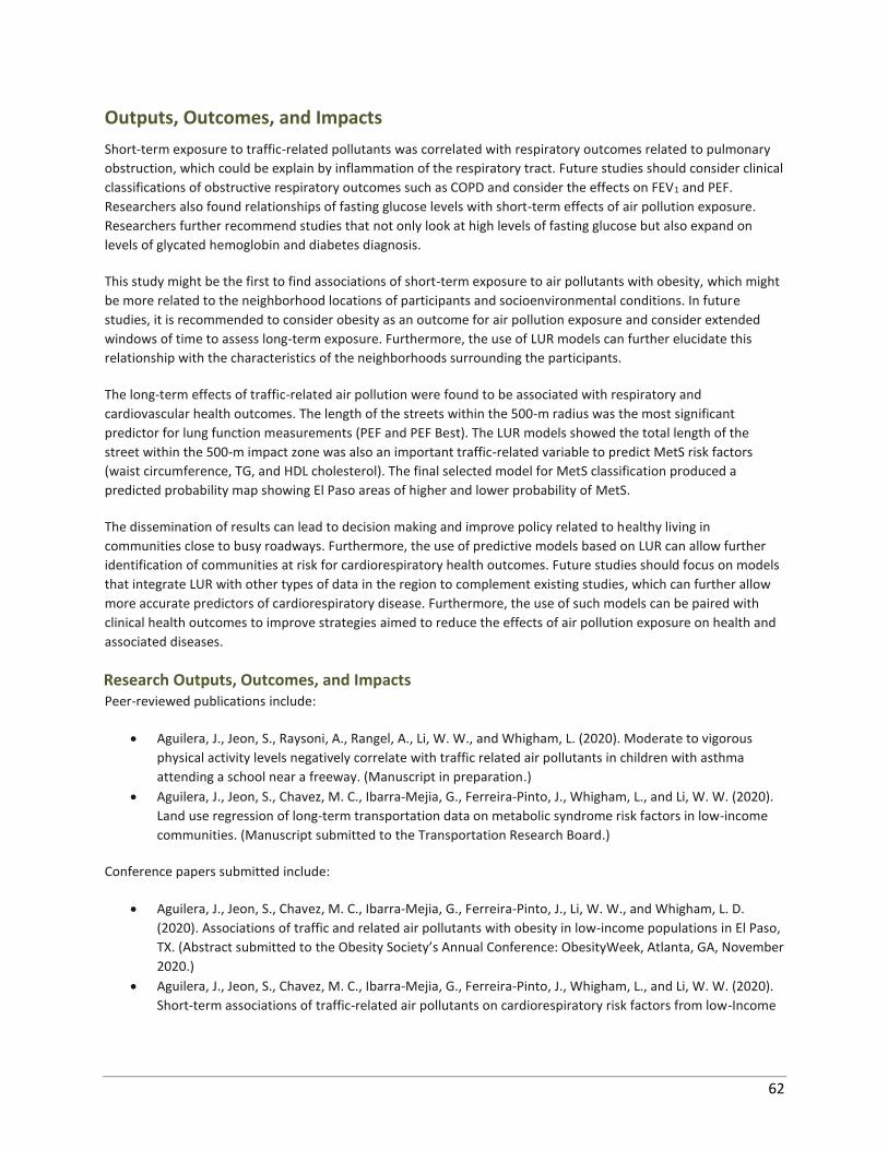
62

Outputs, Outcomes, and Impacts

Short-term exposure to traffic-related pollutants was correlated with respiratory outcomes related to pulmonary

obstruction, which could be explain by inflammation of the respiratory tract. Future studies should consider clinical

classifications of obstructive respiratory outcomes such as COPD and consider the effects on FEV1 and PEF.

Researchers also found relationships of fasting glucose levels with short-term effects of air pollution exposure.

Researchers further recommend studies that not only look at high levels of fasting glucose but also expand on

levels of glycated hemoglobin and diabetes diagnosis.

This study might be the first to find associations of short-term exposure to air pollutants with obesity, which might

be more related to the neighborhood locations of participants and socioenvironmental conditions. In future

studies, it is recommended to consider obesity as an outcome for air pollution exposure and consider extended

windows of time to assess long-term exposure. Furthermore, the use of LUR models can further elucidate this

relationship with the characteristics of the neighborhoods surrounding the participants.

The long-term effects of traffic-related air pollution were found to be associated with respiratory and

cardiovascular health outcomes. The length of the streets within the 500-m radius was the most significant

predictor for lung function measurements (PEF and PEF Best). The LUR models showed the total length of the

street within the 500-m impact zone was also an important traffic-related variable to predict MetS risk factors

(waist circumference, TG, and HDL cholesterol). The final selected model for MetS classification produced a

predicted probability map showing El Paso areas of higher and lower probability of MetS.

The dissemination of results can lead to decision making and improve policy related to healthy living in

communities close to busy roadways. Furthermore, the use of predictive models based on LUR can allow further

identification of communities at risk for cardiorespiratory health outcomes. Future studies should focus on models

that integrate LUR with other types of data in the region to complement existing studies, which can further allow

more accurate predictors of cardiorespiratory disease. Furthermore, the use of such models can be paired with

clinical health outcomes to improve strategies aimed to reduce the effects of air pollution exposure on health and

associated diseases.

Research Outputs, Outcomes, and Impacts Peer-reviewed publications include:

• Aguilera, J., Jeon, S., Raysoni, A., Rangel, A., Li, W. W., and Whigham, L. (2020). Moderate to vigorous

physical activity levels negatively correlate with traffic related air pollutants in children with asthma

attending a school near a freeway. (Manuscript in preparation.)

• Aguilera, J., Jeon, S., Chavez, M. C., Ibarra-Mejia, G., Ferreira-Pinto, J., Whigham, L., and Li, W. W. (2020).

Land use regression of long-term transportation data on metabolic syndrome risk factors in low-income

communities. (Manuscript submitted to the Transportation Research Board.)

Conference papers submitted include:

• Aguilera, J., Jeon, S., Chavez, M. C., Ibarra-Mejia, G., Ferreira-Pinto, J., Li, W. W., and Whigham, L. D.

(2020). Associations of traffic and related air pollutants with obesity in low-income populations in El Paso,

TX. (Abstract submitted to the Obesity Society’s Annual Conference: ObesityWeek, Atlanta, GA, November

2020.)


Short-term associations of traffic-related air pollutants on cardiorespiratory risk factors from low-Income

63

populations in El Paso, TX. (Abstract submitted to the Transportation, Environment, and Energy: An

Integrated Research Symposium, Transportation Research Board, Denver, CO, July 2020.)


Land use regression modeling to assess effects of long-term transportation data on metabolic syndrome

risk factors of low-income communities, TX. (Abstract submitted to the Transportation, Environment, and

Energy: An Integrated Research Symposium, Transportation Research Board, Denver, CO, July 2020.)


Short-term associations of traffic-related air pollutants on cardiorespiratory risk factors from low-income

populations in El Paso, TX. (Abstract submitted to and accepted by the second Transportation, Air Quality,

and Health Symposium, Riverside, CA, May 2020.)

Presentations at conferences and technical meetings include:

• Aguilera, J. (October 2019). Moderate to vigorous physical activity levels negatively correlate with traffic

related air pollutants in children with asthma attending a school near a freeway. Stanford Postdoctoral

Recruitment Initiative in Sciences and Medicine presentation, Stanford, CA.

• Aguilera, J. Association of traffic and related air pollutants on cardiorespiratory risk factors from low-

income populations in El Paso. The University of Texas at El Paso, El Paso, TX.

• Aguilera, J. (March 2020). General aspects of COVID-19: Airborne transmission, immune response, and

chronic disease risk. Health Clinic Day, Consulate General of Mexico in El Paso, El Paso, TX.

• Aguilera, J. (July 2020). Short-term effects of traffic related air pollution on cardiorespiratory outcomes

among low-income residents from El Paso, TX. Joint Advisory Committee for the Improvement of Air

Quality in the Ciudad Juárez, Chihuahua/El Paso, Texas/Doña Ana County, New México Air Basin (virtual).

• Jeon, S. (July 2020). Land use regression modeling to assess effects of long-term transportation data on

metabolic syndrome risk factors of low-income communities in El Paso, TX. Joint Advisory Committee for

the Improvement of Air Quality in the Ciudad Juárez, Chihuahua/El Paso, Texas/Doña Ana County, New

México Air Basin (virtual).

• Aguilera, J. (August 2020). Land use regression of long-term transportation data on metabolic syndrome

risk factors in low-income communities. Fundación Best monthly seminar in Ciudad Juarez.

• Results and main findings (the predicted probability map for MetS) were shared with the public in a

virtual Joint Advisory Committee meeting.

Technology Transfer Outputs, Outcomes, and Impacts This project had the following technology transfer outputs, outcomes, and impacts:

• Air quality data were acquired from TCEQ’s CAMSs, including hourly air pollutant data.

• Time-integrated air pollutant data of 24-, 48-, 72-, and 96-hr averages were processed for each subject.

• Short-term pollution exposures and long-term transportation data were extracted using GIS mapping.

• GIS layers from Census.gov and the El Paso Metropolitan Planning Organization were used.

• Statistical code for LUR modeling was developed.

• The interpolation technique was applied to produce a predicted probability map.

• Software was used as part of this study including R and ArcGIS Pro.

Education and Workforce Development Outputs, Outcomes, and Impacts This project had the following education and workforce development outputs, outcomes, and impacts:

• This project supported a doctoral student from Health Science at UTEP as a research associate.

64

• The project was conducted as part of a doctoral dissertation in the Interdisciplinary Health Sciences

program at UTEP.

• An undergraduate student from the Department of Civil Engineering at UTEP was involved in the project.

• Training and education in application of GIS information to transportation data were conducted.

65

References

Adam, M., Schikowski, T., Carsin, A. E., Cai, Y., Jacquemin, B., Sanchez, M., ... Sugiri, D. (2015). Adult lung function

and long-term air pollution exposure. ESCAPE: A multicentre cohort study and meta-analysis. European respiratory

journal, 45(1), 38-50.

Aguilera, J. (2016). Prevalence of risk factors for metabolic syndrome in uninsured Hispanic adults from low income

communities in El Paso, Texas. The University of Texas at El Paso.

Alvarez, H. A. O., Myers, O. B., Weigel, M., and Armijos, R. X. (2018). The value of using seasonality and

meteorological variables to model intra-urban PM2.5 variation. Atmospheric environment, 182, 1-8.

Amini, H., Yunesian, M., Hosseini, V., Schindler, C., Henderson, S. B., and Künzli, N. (2017). A systematic review of

land use regression models for volatile organic compounds. Atmospheric environment, 171, 1-16.

Andersen, I. (1972). Relationships between outdoor and indoor air pollution. Atmospheric environment (1967),

6(4), 275-278.

Atkinson, R. W., Fuller, G. W., Anderson, H. R., Harrison, R. M., and Armstrong, B. (2010). Urban ambient particle

metrics and health: A time-series analysis. Epidemiology, 21(4), 501-511.

Barone-Adesi, F., Dent, J. E., Dajnak, D., Beevers, S., Anderson, H. R., Kelly, F. J., ... Whincup, P. H. (2015). Long-term

exposure to primary traffic pollutants and lung function in children: Cross-sectional study and meta-analysis. PloS

one, 10(11), e0142565.

Barraza-Villarreal, A., Sunyer, J., Hernandez-Cadena, L., Escamilla-Nuñez, M. C., Sienra-Monge, J. J., Ramírez-

Aguilar, M., ... Olin, A. C. (2008). Air pollution, airway inflammation, and lung function in a cohort study of Mexico

City schoolchildren. Environmental health perspectives, 116(6), 832-838.

Bell, G., Mora, S., Greenland, P., Tsai, M., Gill, E., and Kaufman, J. D. (2017). Association of air pollution exposures

with high-density lipoprotein cholesterol and particle number: The multi-ethnic study of atherosclerosis.

Arteriosclerosis, thrombosis, and vascular biology, 37(5), 976-982.

Bowe, B., Xie, Y., Li, T., Yan, Y., Xian, H., and Al-Aly, Z. (2018). The 2016 global and national burden of diabetes

mellitus attributable to PM 2.5 air pollution. The Lancet Planetary Health, 2(7), e301-e312.

Brulle, R. J., and Pellow, D. N. (2006). Environmental justice: Human health and environmental inequalities. Annu.

Rev. Public Health, 27, 103-124.

Cadelis, G., Tourres, R., and Molinie, J. (2014). Short-term effects of the particulate pollutants contained in Saharan

dust on the visits of children to the emergency department due to asthmatic conditions in Guadeloupe (French

Archipelago of the Caribbean). PloS one, 9(3).

Cai, Y., Zhang, B., Ke, W., Feng, B., Lin, H., Xiao, J., ... Yang, Z. (2016). Associations of short-term and long-term

exposure to ambient air pollutants with hypertension: A systematic review and meta-analysis. Hypertension, 68(1),

62-70.

Chen, J.-C., and Schwartz, J. (2008). Metabolic syndrome and inflammatory responses to long-term particulate air

pollutants. Environmental health perspectives, 116(5), 612-617.

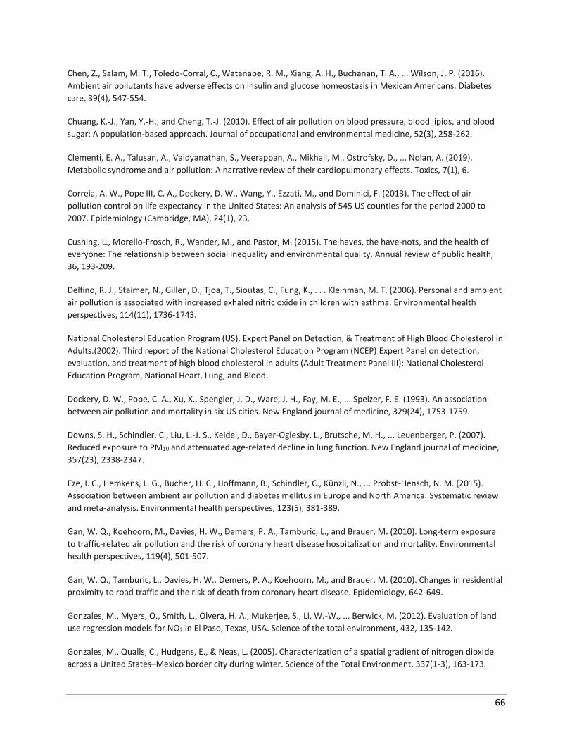
66

Chen, Z., Salam, M. T., Toledo-Corral, C., Watanabe, R. M., Xiang, A. H., Buchanan, T. A., ... Wilson, J. P. (2016).

Ambient air pollutants have adverse effects on insulin and glucose homeostasis in Mexican Americans. Diabetes

care, 39(4), 547-554.

Chuang, K.-J., Yan, Y.-H., and Cheng, T.-J. (2010). Effect of air pollution on blood pressure, blood lipids, and blood

sugar: A population-based approach. Journal of occupational and environmental medicine, 52(3), 258-262.

Clementi, E. A., Talusan, A., Vaidyanathan, S., Veerappan, A., Mikhail, M., Ostrofsky, D., ... Nolan, A. (2019).

Metabolic syndrome and air pollution: A narrative review of their cardiopulmonary effects. Toxics, 7(1), 6.

Correia, A. W., Pope III, C. A., Dockery, D. W., Wang, Y., Ezzati, M., and Dominici, F. (2013). The effect of air

pollution control on life expectancy in the United States: An analysis of 545 US counties for the period 2000 to

2007. Epidemiology (Cambridge, MA), 24(1), 23.

Cushing, L., Morello-Frosch, R., Wander, M., and Pastor, M. (2015). The haves, the have-nots, and the health of

everyone: The relationship between social inequality and environmental quality. Annual review of public health,

36, 193-209.

Delfino, R. J., Staimer, N., Gillen, D., Tjoa, T., Sioutas, C., Fung, K., . . . Kleinman, M. T. (2006). Personal and ambient

air pollution is associated with increased exhaled nitric oxide in children with asthma. Environmental health

perspectives, 114(11), 1736-1743.

National Cholesterol Education Program (US). Expert Panel on Detection, & Treatment of High Blood Cholesterol in

Adults.(2002). Third report of the National Cholesterol Education Program (NCEP) Expert Panel on detection,

evaluation, and treatment of high blood cholesterol in adults (Adult Treatment Panel III): National Cholesterol

Education Program, National Heart, Lung, and Blood.

Dockery, D. W., Pope, C. A., Xu, X., Spengler, J. D., Ware, J. H., Fay, M. E., ... Speizer, F. E. (1993). An association

between air pollution and mortality in six US cities. New England journal of medicine, 329(24), 1753-1759.

Downs, S. H., Schindler, C., Liu, L.-J. S., Keidel, D., Bayer-Oglesby, L., Brutsche, M. H., ... Leuenberger, P. (2007).

Reduced exposure to PM10 and attenuated age-related decline in lung function. New England journal of medicine,

357(23), 2338-2347.

Eze, I. C., Hemkens, L. G., Bucher, H. C., Hoffmann, B., Schindler, C., Künzli, N., ... Probst-Hensch, N. M. (2015).

Association between ambient air pollution and diabetes mellitus in Europe and North America: Systematic review

and meta-analysis. Environmental health perspectives, 123(5), 381-389.

Gan, W. Q., Koehoorn, M., Davies, H. W., Demers, P. A., Tamburic, L., and Brauer, M. (2010). Long-term exposure

to traffic-related air pollution and the risk of coronary heart disease hospitalization and mortality. Environmental

health perspectives, 119(4), 501-507.

Gan, W. Q., Tamburic, L., Davies, H. W., Demers, P. A., Koehoorn, M., and Brauer, M. (2010). Changes in residential

proximity to road traffic and the risk of death from coronary heart disease. Epidemiology, 642-649.

Gonzales, M., Myers, O., Smith, L., Olvera, H. A., Mukerjee, S., Li, W.-W., ... Berwick, M. (2012). Evaluation of land

use regression models for NO2 in El Paso, Texas, USA. Science of the total environment, 432, 135-142.

Gonzales, M., Qualls, C., Hudgens, E., & Neas, L. (2005). Characterization of a spatial gradient of nitrogen dioxide

across a United States–Mexico border city during winter. Science of the Total Environment, 337(1-3), 163-173.

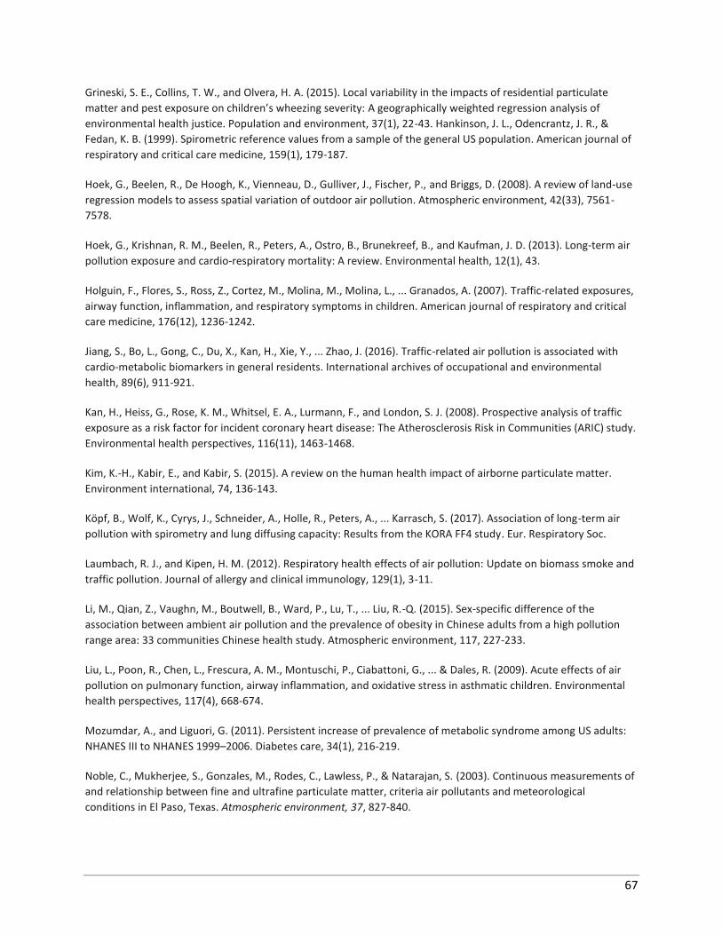
67

Grineski, S. E., Collins, T. W., and Olvera, H. A. (2015). Local variability in the impacts of residential particulate

matter and pest exposure on children’s wheezing severity: A geographically weighted regression analysis of

environmental health justice. Population and environment, 37(1), 22-43. Hankinson, J. L., Odencrantz, J. R., &

Fedan, K. B. (1999). Spirometric reference values from a sample of the general US population. American journal of

respiratory and critical care medicine, 159(1), 179-187.

Hoek, G., Beelen, R., De Hoogh, K., Vienneau, D., Gulliver, J., Fischer, P., and Briggs, D. (2008). A review of land-use

regression models to assess spatial variation of outdoor air pollution. Atmospheric environment, 42(33), 7561-

7578.

Hoek, G., Krishnan, R. M., Beelen, R., Peters, A., Ostro, B., Brunekreef, B., and Kaufman, J. D. (2013). Long-term air

pollution exposure and cardio-respiratory mortality: A review. Environmental health, 12(1), 43.

Holguin, F., Flores, S., Ross, Z., Cortez, M., Molina, M., Molina, L., ... Granados, A. (2007). Traffic-related exposures,

airway function, inflammation, and respiratory symptoms in children. American journal of respiratory and critical

care medicine, 176(12), 1236-1242.

Jiang, S., Bo, L., Gong, C., Du, X., Kan, H., Xie, Y., ... Zhao, J. (2016). Traffic-related air pollution is associated with

cardio-metabolic biomarkers in general residents. International archives of occupational and environmental

health, 89(6), 911-921.

Kan, H., Heiss, G., Rose, K. M., Whitsel, E. A., Lurmann, F., and London, S. J. (2008). Prospective analysis of traffic

exposure as a risk factor for incident coronary heart disease: The Atherosclerosis Risk in Communities (ARIC) study.

Environmental health perspectives, 116(11), 1463-1468.

Kim, K.-H., Kabir, E., and Kabir, S. (2015). A review on the human health impact of airborne particulate matter.

Environment international, 74, 136-143.

Köpf, B., Wolf, K., Cyrys, J., Schneider, A., Holle, R., Peters, A., ... Karrasch, S. (2017). Association of long-term air

pollution with spirometry and lung diffusing capacity: Results from the KORA FF4 study. Eur. Respiratory Soc.

Laumbach, R. J., and Kipen, H. M. (2012). Respiratory health effects of air pollution: Update on biomass smoke and

traffic pollution. Journal of allergy and clinical immunology, 129(1), 3-11.

Li, M., Qian, Z., Vaughn, M., Boutwell, B., Ward, P., Lu, T., ... Liu, R.-Q. (2015). Sex-specific difference of the

association between ambient air pollution and the prevalence of obesity in Chinese adults from a high pollution

range area: 33 communities Chinese health study. Atmospheric environment, 117, 227-233.

Liu, L., Poon, R., Chen, L., Frescura, A. M., Montuschi, P., Ciabattoni, G., ... & Dales, R. (2009). Acute effects of air

pollution on pulmonary function, airway inflammation, and oxidative stress in asthmatic children. Environmental

health perspectives, 117(4), 668-674.

Mozumdar, A., and Liguori, G. (2011). Persistent increase of prevalence of metabolic syndrome among US adults:

NHANES III to NHANES 1999–2006. Diabetes care, 34(1), 216-219.

Noble, C., Mukherjee, S., Gonzales, M., Rodes, C., Lawless, P., & Natarajan, S. (2003). Continuous measurements of

and relationship between fine and ultrafine particulate matter, criteria air pollutants and meteorological

conditions in El Paso, Texas. Atmospheric environment, 37, 827-840.

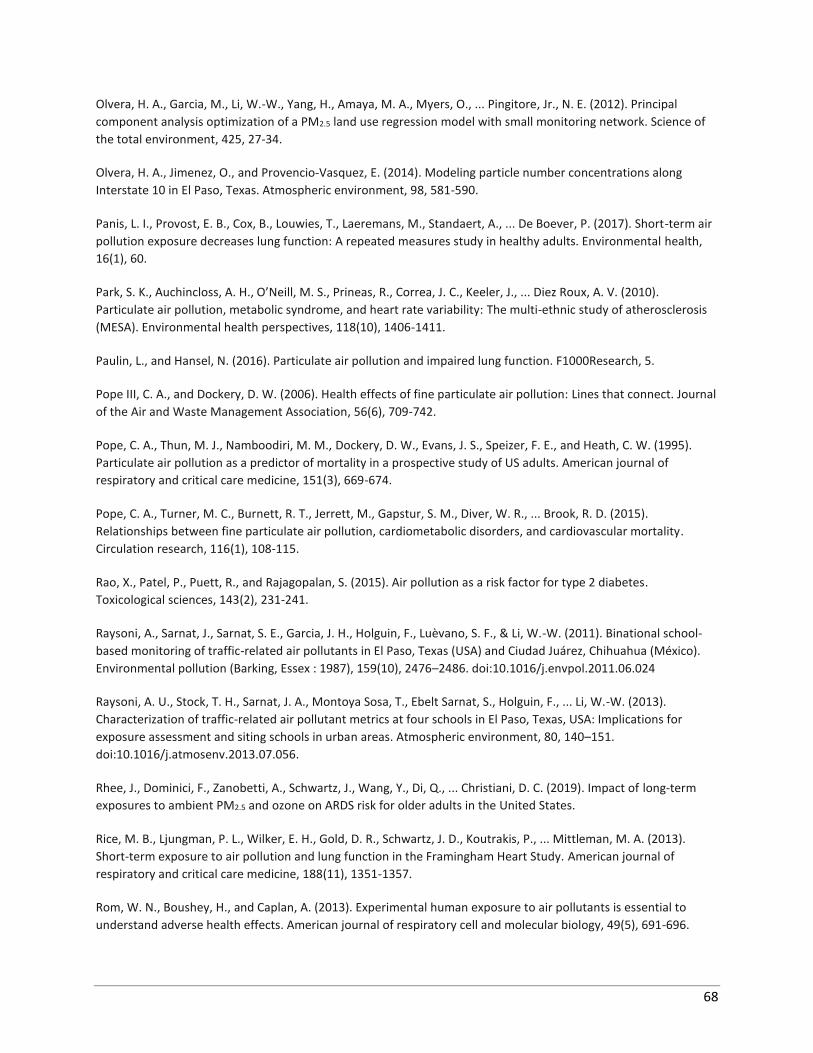
68

Olvera, H. A., Garcia, M., Li, W.-W., Yang, H., Amaya, M. A., Myers, O., ... Pingitore, Jr., N. E. (2012). Principal

component analysis optimization of a PM2.5 land use regression model with small monitoring network. Science of

the total environment, 425, 27-34.

Olvera, H. A., Jimenez, O., and Provencio-Vasquez, E. (2014). Modeling particle number concentrations along

Interstate 10 in El Paso, Texas. Atmospheric environment, 98, 581-590.

Panis, L. I., Provost, E. B., Cox, B., Louwies, T., Laeremans, M., Standaert, A., ... De Boever, P. (2017). Short-term air

pollution exposure decreases lung function: A repeated measures study in healthy adults. Environmental health,

16(1), 60.

Park, S. K., Auchincloss, A. H., O’Neill, M. S., Prineas, R., Correa, J. C., Keeler, J., ... Diez Roux, A. V. (2010).

Particulate air pollution, metabolic syndrome, and heart rate variability: The multi-ethnic study of atherosclerosis

(MESA). Environmental health perspectives, 118(10), 1406-1411.

Paulin, L., and Hansel, N. (2016). Particulate air pollution and impaired lung function. F1000Research, 5.

Pope III, C. A., and Dockery, D. W. (2006). Health effects of fine particulate air pollution: Lines that connect. Journal

of the Air and Waste Management Association, 56(6), 709-742.

Pope, C. A., Thun, M. J., Namboodiri, M. M., Dockery, D. W., Evans, J. S., Speizer, F. E., and Heath, C. W. (1995).

Particulate air pollution as a predictor of mortality in a prospective study of US adults. American journal of


Pope, C. A., Turner, M. C., Burnett, R. T., Jerrett, M., Gapstur, S. M., Diver, W. R., ... Brook, R. D. (2015).

Relationships between fine particulate air pollution, cardiometabolic disorders, and cardiovascular mortality.

Circulation research, 116(1), 108-115.

Rao, X., Patel, P., Puett, R., and Rajagopalan, S. (2015). Air pollution as a risk factor for type 2 diabetes.

Toxicological sciences, 143(2), 231-241.

Raysoni, A., Sarnat, J., Sarnat, S. E., Garcia, J. H., Holguin, F., Luèvano, S. F., & Li, W.-W. (2011). Binational school-

based monitoring of traffic-related air pollutants in El Paso, Texas (USA) and Ciudad Juárez, Chihuahua (México).

Environmental pollution (Barking, Essex : 1987), 159(10), 2476–2486. doi:10.1016/j.envpol.2011.06.024

Raysoni, A. U., Stock, T. H., Sarnat, J. A., Montoya Sosa, T., Ebelt Sarnat, S., Holguin, F., ... Li, W.-W. (2013).

Characterization of traffic-related air pollutant metrics at four schools in El Paso, Texas, USA: Implications for

exposure assessment and siting schools in urban areas. Atmospheric environment, 80, 140–151.

doi:10.1016/j.atmosenv.2013.07.056.

Rhee, J., Dominici, F., Zanobetti, A., Schwartz, J., Wang, Y., Di, Q., ... Christiani, D. C. (2019). Impact of long-term

exposures to ambient PM2.5 and ozone on ARDS risk for older adults in the United States.

Rice, M. B., Ljungman, P. L., Wilker, E. H., Gold, D. R., Schwartz, J. D., Koutrakis, P., ... Mittleman, M. A. (2013).

Short-term exposure to air pollution and lung function in the Framingham Heart Study. American journal of


Rom, W. N., Boushey, H., and Caplan, A. (2013). Experimental human exposure to air pollutants is essential to

understand adverse health effects. American journal of respiratory cell and molecular biology, 49(5), 691-696.

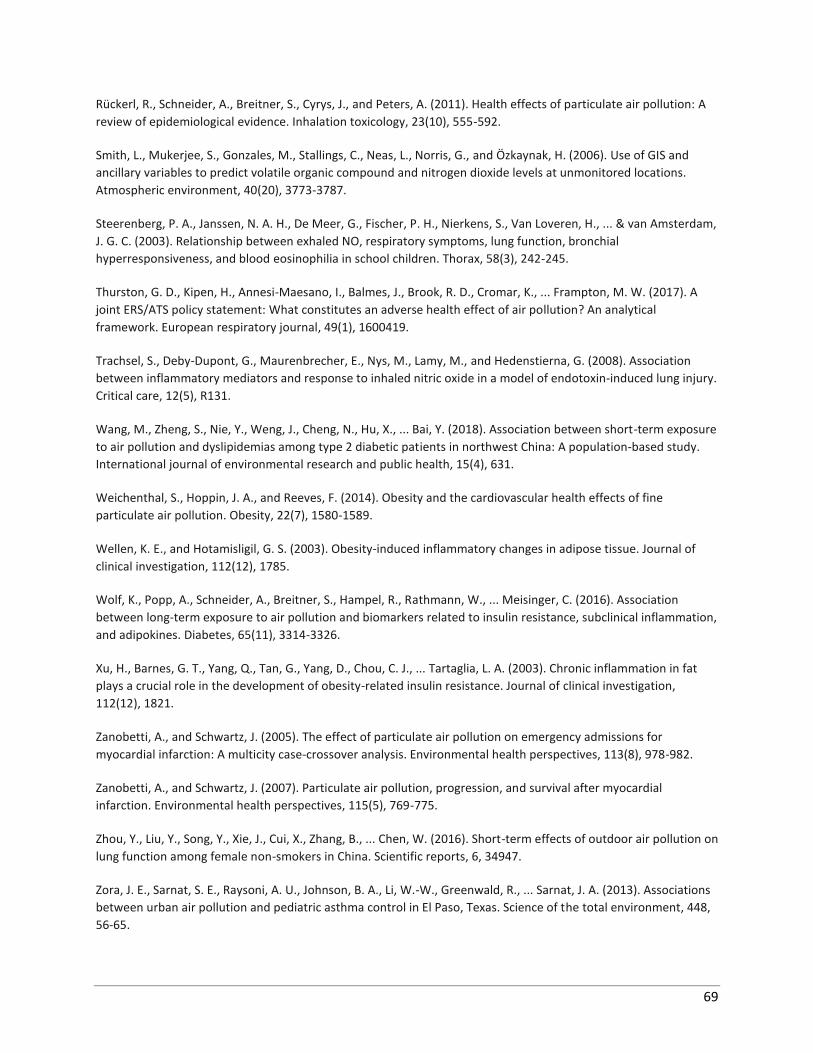
69

Rückerl, R., Schneider, A., Breitner, S., Cyrys, J., and Peters, A. (2011). Health effects of particulate air pollution: A

review of epidemiological evidence. Inhalation toxicology, 23(10), 555-592.

Smith, L., Mukerjee, S., Gonzales, M., Stallings, C., Neas, L., Norris, G., and Özkaynak, H. (2006). Use of GIS and

ancillary variables to predict volatile organic compound and nitrogen dioxide levels at unmonitored locations.

Atmospheric environment, 40(20), 3773-3787.

Steerenberg, P. A., Janssen, N. A. H., De Meer, G., Fischer, P. H., Nierkens, S., Van Loveren, H., ... & van Amsterdam,

J. G. C. (2003). Relationship between exhaled NO, respiratory symptoms, lung function, bronchial

hyperresponsiveness, and blood eosinophilia in school children. Thorax, 58(3), 242-245.

Thurston, G. D., Kipen, H., Annesi-Maesano, I., Balmes, J., Brook, R. D., Cromar, K., ... Frampton, M. W. (2017). A

joint ERS/ATS policy statement: What constitutes an adverse health effect of air pollution? An analytical

framework. European respiratory journal, 49(1), 1600419.

Trachsel, S., Deby-Dupont, G., Maurenbrecher, E., Nys, M., Lamy, M., and Hedenstierna, G. (2008). Association

between inflammatory mediators and response to inhaled nitric oxide in a model of endotoxin-induced lung injury.

Critical care, 12(5), R131.

Wang, M., Zheng, S., Nie, Y., Weng, J., Cheng, N., Hu, X., ... Bai, Y. (2018). Association between short-term exposure

to air pollution and dyslipidemias among type 2 diabetic patients in northwest China: A population-based study.

International journal of environmental research and public health, 15(4), 631.

Weichenthal, S., Hoppin, J. A., and Reeves, F. (2014). Obesity and the cardiovascular health effects of fine

particulate air pollution. Obesity, 22(7), 1580-1589.

Wellen, K. E., and Hotamisligil, G. S. (2003). Obesity-induced inflammatory changes in adipose tissue. Journal of

clinical investigation, 112(12), 1785.

Wolf, K., Popp, A., Schneider, A., Breitner, S., Hampel, R., Rathmann, W., ... Meisinger, C. (2016). Association

between long-term exposure to air pollution and biomarkers related to insulin resistance, subclinical inflammation,

and adipokines. Diabetes, 65(11), 3314-3326.

Xu, H., Barnes, G. T., Yang, Q., Tan, G., Yang, D., Chou, C. J., ... Tartaglia, L. A. (2003). Chronic inflammation in fat

plays a crucial role in the development of obesity-related insulin resistance. Journal of clinical investigation,

112(12), 1821.

Zanobetti, A., and Schwartz, J. (2005). The effect of particulate air pollution on emergency admissions for

myocardial infarction: A multicity case-crossover analysis. Environmental health perspectives, 113(8), 978-982.

Zanobetti, A., and Schwartz, J. (2007). Particulate air pollution, progression, and survival after myocardial

infarction. Environmental health perspectives, 115(5), 769-775.

Zhou, Y., Liu, Y., Song, Y., Xie, J., Cui, X., Zhang, B., ... Chen, W. (2016). Short-term effects of outdoor air pollution on

lung function among female non-smokers in China. Scientific reports, 6, 34947.

Zora, J. E., Sarnat, S. E., Raysoni, A. U., Johnson, B. A., Li, W.-W., Greenwald, R., ... Sarnat, J. A. (2013). Associations

between urban air pollution and pediatric asthma control in El Paso, Texas. Science of the total environment, 448,

56-65.

70

Zou, B., Wilson, J. G., Zhan, F. B., and Zeng, Y. (2009). Air pollution exposure assessment methods utilized in

epidemiological studies. Journal of environmental monitoring, 11(3), 475-490.

Documents

ASSOCIATION OF TRAFFIC AND RELATED AIR POLLUTANTS …