Embed Size (px)
Citation preview

ASSIGNMENT COVER SHEET
Student Name: __________________________________________
Student ID: __________________________________________
Unit Name: __________________________________________
Lecturer’s Name: __________________________________________
Due Date: __________________________________________
Date Submitted: __________________________________________
DECLARATION
I have read and understood Curtin’s policy on plagiarism, and, except where indicated, this assignment is my own work and has not been submitted for assessment in another unit or course. I have given appropriate references where ideas have been taken from the published or unpublished work of others, and clearly acknowledge where blocks of text have been taken from other sources.
I have retained a copy of the assignment for my own records.
________________________________________
[Signature of student]
For Lecturer’s Use Only:
Overall Mark: ________ out of a total of _________ Percentage:
Lecturer’s Comments:
Lecturer’s Name: Date Returned:
Sutthisrisaarng Pholpark
17682974
Geophysical Data Processing 612 (Petroleum)
Sasha S.
7 November 2014
7 November 2014
Sutthisrisaarng Pholpark
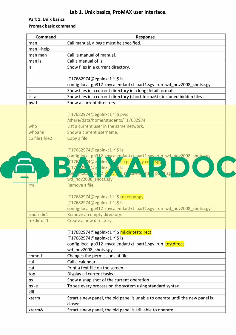
Lab 1. Unix basics, ProMAX user interface.
Part 1. Unix basics
Promax basic command
Command Response
man Call manual, a page must be specified.
man --help
man man Call a manual of manual.
man ls Call a manual of ls.
ls Show files in a current directory.
[T17682974@egplnxc1 ~]$ ls
config-local-gp312 mycalendar.txt part1.sgy run wd_nov2008_shots.sgy
ls Show files in a current directory in a long detail format.
ls -a Show files in a current directory (short forma6t), included hidden files .
pwd Show a current directory.
[T17682974@egplnxc1 ~]$ pwd
/share/data/home/students/T17682974
who List a current user in the same network.
whoami Show a current username.
cp file1 file2 Copy a file.
[T17682974@egplnxc1 ~]$ ls
config-local-gp312 mycalendar.txt part1.sgy run wd_nov2008_shots.sgy
[T17682974@egplnxc1 ~]$ cp part1.sgy copy.sgy
[T17682974@egplnxc1 ~]$ ls
config-local-gp312 copy.sgy mycalendar.txt part1.sgy run
wd_nov2008_shots.sgy
rm Remove a file
[T17682974@egplnxc1 ~]$ rm copy.sgy
[T17682974@egplnxc1 ~]$ ls
config-local-gp312 mycalendar.txt part1.sgy run wd_nov2008_shots.sgy
rmdir dir1 Remove an empty directory.
mkdir dir1 Create a new directory.
[T17682974@egplnxc1 ~]$ mkdir testdirect
[T17682974@egplnxc1 ~]$ ls
config-local-gp312 mycalendar.txt part1.sgy run testdirect
wd_nov2008_shots.sgy
chmod Changes the permissions of file.
cal Call a calendar.
cat Print a text file on the screen
top Display all current tasks.
ps Show a snap shot of the current operation.
ps -e To see every process on the system using standard syntax
kill
xterm Strart a new panel, the old panel is unable to operate until the new panel is
closed.
xterm& Strart a new panel, the old panel is still able to operate.

- Create text file named ‘mycalendar.txt’ containing calendar of this month; display content of the file on your screen
[T17682974@egplnxc1 ~]$ cal > mycalendar.txt
[T17682974@egplnxc1 ~]$ cat mycalendar.txt
August 2014
Su Mo Tu We Th Fr Sa
1 2
3 4 5 6 7 8 9
10 11 12 13 14 15 16
17 18 19 20 21 22 23
24 25 26 27 28 29 30
31
- Change permissions for that file; allow all users to read the content
[T17682974@egplnxc1 ~]$ chmod 755 mycalendar.txt
Part 2. ProMAX user interface
Marine seismic
- Display raw data
> STEP 1/3: Create line
>> STEP2/3: Create flow
>>> STEP3/3: Select operation method in flow, the execute
- Display raw data in WA/WT, WT, and greyscale mode.
Grayscale mode
WA (Display only maximum amplitude)
WT(Display only traces, no maximum
amplitude highlighted)
WA/WT(Combined WA and WT)
Comment: We can also display traces in color mode.

- Annotate axis using FFID and CHAN
- Answer the following questions:
a. What are the main parameters of file, i.e. sampling interval, number of samples (see the
log file)?
# Traces per Ensemble .............. = 230
# Auxiliary Traces per Ensemble .... = 51614
Sample interval (micro sec) ........ = 6000
Recording sample interval .......... = 2000
# samples per trace ................ = 668
# recording samples per trace ...... = 4097
Data sample format ................. = 4 Byte IBM floating point
b. Which trace headers have some defined values?
FFID: Field File Identification Number , increases
with #of shots
CHAN: #of channel
OFFSET
AOFFSET
CDP: Common Depth Point
CDP_X
CDP_Y
DEPTH
FILE_NO
SEQNO
SOURCE
SOU_H2OD
TFULL_E
TLIVE_E
TOTSTAT
TRACENO
TRC_TYPE
TR_FOLD
c. Identify main components of the wave field.

Land seismic
- Answer the following questions:
a. What are the main parameters of file, i.e. sampling interval, number of samples (see the
log file)?
# Traces per Ensemble .............. = 156
# Auxiliary Traces per Ensemble .... = 51614
Sample interval (micro sec) ........ = 1000
Recording sample interval .......... = 0
# samples per trace ................ = 3001
# recording samples per trace ...... = 1250
Data sample format ................. = 4 Byte IBM floating point
b. Which trace headers have some defined values?
b. Which trace headers have some defined values?
FFID: Field File Identification Number , increases
with #of shots
CHAN: #of channel
OFFSET
AOFFSET
CDP: Common Depth Point
CDP_X,CDP_Y
LINE_NO
REC_X,REC_XD
FILE_NO
SEQNO
SOURCE
SOU_X,SOU_XD
SOU_H2OD
TFULL_E
TFULL_S
TLIVE_E
TLIVE_S
TRACENO
TRC_TYPE
TR_FOLD
c. Identify main components of the wave field.

Lab 2: Geometry
Objective
Learn to set geometry for raw seismic data and perform quality control after geometry is
assigned.
FLOWS
1/5 Load seismic data to the database
Flow: 010 – SEGY Input
SEG-Y Input - read all traces from ‘’part1.sgy”
Disk Data Output – Stored data in the database (at the current flow) name “raw data”
The loaded data can be viewed by clicking
‘datasets’ tab, then use MB2 to click ‘raw data’.
If use MB3, Promax will show history of the file.
2/5 Creating database files
Flow: 020 – Extract DB Files
The main function of this flow is to extract headers from ‘raw data’ in order to generate Promax database entries.
Since trace headers are only used for DB files
generation, click ‘YES’ at ‘Process trace headers
only’.

3/5 Assigning geometry
Flow: 030 – Geometry
The only one function of this flow is to generate ‘2D Marine Geometry Spreadsheet’. The picture below has been taken from GP312, lecture2 geometry.
Number of channels in the streamer: 230
Minimum inline offset: 130 m
Crossline source offset: 0 m
Receiver group interval 12.5 m
Source interval: 50 m
Streamer towing depth: 8 m
Source towing depth: 6 m
Nominal sail line azimuth: 0°
Use ‘matching pattern’ midpoints assignment method.
After flow ‘030 – Geometry’ has been executed, the geometry spreadsheet will show
up.
Geometry assignment sequence (menu items) as provided in the lab instructions are:
1. Setup – enter parameters
2. Sources – coordinates of sources
3. Pattern – define pattern of recievers
4. Bin – assign midpoints, bin and finalize database
5. QC the results – show survey pattern
Setup
Sources
Patterns

Binning
All parameters assigned above are used to construct a binning grid in binning process.
QC the results - using TarceQC create cross-plot SIN
vs REC_Y coloured according to OFFSET (View->View
All->XY Graph).
Explanation: Since each header of raw
seismic trace does not contain geometry
information, geometry information is
needed to be assigned before a processing
in further steps e.g. stacking. In order to
create a survey grid regarding to survey
geometry, important survey parameters are
binned together. After binning process, the
QC results are obtained from the plot SIN vs
REC_Y coloured according to OFFSET.
Overall, the plot shows geometry of survey
lines. Each line indicates shot locations
obtained from the same SIN or source index
number which is an assigned number for
each shot point. The highest number of
each line in Y-axis indicates the minimum
inline offset. Every move of a source
position (source interval) increases SIN
number one step (+1) until 208 (the last
shot). In addition, as source interval is 50m,
the move of source also increases the
minimum inline offset by 50m.
Note: Source live number is obtained from
the field data but for Sin we created it in
geometry assignment process.
4/5 Updating trace headers with correct values
In step 3/5, geometry spread sheet was created, however, the geometry has not been applied to
the data set ‘raw data’. Hence, the main purpose of this flow is to apply the geometry to the data set.
Flow: 040 – Inline geometry
After assigned geometry for the dataset, dataset
information shows that geometry matches database and
trace number matches database.

4/5 QC
1. Sort data in SOURCE:AOFFSET order, tune display parameters to see 5 ensembles each time
(displayed in grayscale), use FFID and OFFSET to annotate traces
2. Make sure that tools used for travel time approximation with a straight line and hyperbola show
realistic values for direct wave and bottom reflection.
Note: the average velocity of direct wave is 1534.6 m/s and the average velocity of bottom
reflection is 1487.4 m/s.
3. Pick direct wave and project on a first ensemble and project to all of them. It must follow direct
wave on all ensembles, scroll till the end of the line.
In order to pick direct wave and project the pick to ensembles, “Pick Miscellaneous Time Gates function is used”. The method is shown below.

After project the direct wave pick to all ensembles, all of them follow the projected lines which
indicates that assigned geometry works properly.
4. Resort data in CDP:AOFFSET order, explain changes in number of traces per ensemble in respect
to SOURCE:AOFFSET.
SOURCE:AOFFSET - #trace = 230 traces per ensemble (constant number thorough all of SIN)
CDP:AOFFSET- #trace = traces per ensemble increasing as the number of fold increasing as in the
fold diagram below. Number of traces start from 1 at CDP1, increasing up to 29 and then decreasing
to 1 afterwards.
Hence, in the case of CDP:AOFFSET sorting, #trace in each CDP ensemble depends on #fold while
SOURCE:AOFFSET sorting #trace in SIN ensemble is a constant number 230 traces per ensemble.
#traces increses with #fold
Fold diagram